Journal of Financial Economics 17 (1986) 357-390. North-Holland PREDICI’ING RETURNS IN THE STOCK AND BOND MARKETS* Donald B. KEIM Umcersqvof Pennsyluanla. Phrladeiphla, PA 19104. USA Robert F. STAMBAUGH L’niversity of Chicago, Chicago, IL 6063 7. tiSA Received October 1984. final version received March 1986 Several predetermined variables that reflect levels of bond and stock prices appear to predict returns on common stocks of firms of various sizes, long-term bonds of various default risks. and default-free bonds of various maturities. The returns on small-firm stocks and low-grade bonds are more highly correlated in January than in the rest of the year with previous levels of asset prices. especially prices of small-firm stocks. Seasonality is found in several conditional risk measures, but such seasonality is unlikely to explain, and in some cases is opposite to. the seasonal found in mean returns. 1. Introduction A question of long-standing interest to both academics and practitioners is whether returns on risky assets are predictable. We ask, more specifically, whether there are ex ante observable variables that reliably predict ex post ‘risk premiums’, defined as rates of return in excess of the short-term interest rate. To find that expected risk premiums on many assets change predictably with a few common variables would complement nicely much of modem finance theory. Asset pricing theories often relate (conditional) expected risk premiums to (conditional) covat-iances in models of the form *We thank Nai-fu Chen. Eugene Fama, Wayne Ferson, Michael Gibbons. Jay Ritter, Krishna Ramaswamy, G. William Schwert, and participants in workshops at the University of Chicago, Columbia University, London Business School, Northwestern University, and the University of Pennsylvania for helpful comments. We also thank Eugene Fama for providing some of the data used in the paper. Financial support from the Center for Research in Security Prices and the Institute for Quantitative Research in Finance is gratefully acknowledged. This research was completed while the second author was a Batterymarch Fellow. 0304-405X/86/$3.50 t 1986. Elsevier Science Publishers B.V. (North-Holland)
Transcript
Journal of Financial Economics 17 (1986) 357-390. North-Holland
PREDICI’ING RETURNS IN THE STOCK AND BOND MARKETS*
Donald B. KEIM
Umcersqv of Pennsyluanla. Phrladeiphla, PA 19104. USA
Robert F. STAMBAUGH
L’niversity of Chicago, Chicago, IL 6063 7. tiSA
Received October 1984. final version received March 1986
Several predetermined variables that reflect levels of bond and stock prices appear to predict returns on common stocks of firms of various sizes, long-term bonds of various default risks. and default-free bonds of various maturities. The returns on small-firm stocks and low-grade bonds are more highly correlated in January than in the rest of the year with previous levels of asset prices. especially prices of small-firm stocks. Seasonality is found in several conditional risk measures, but such seasonality is unlikely to explain, and in some cases is opposite to. the seasonal found in mean returns.
1. Introduction
A question of long-standing interest to both academics and practitioners is whether returns on risky assets are predictable. We ask, more specifically, whether there are ex ante observable variables that reliably predict ex post ‘risk premiums’, defined as rates of return in excess of the short-term interest rate.
To find that expected risk premiums on many assets change predictably with a few common variables would complement nicely much of modem finance theory. Asset pricing theories often relate (conditional) expected risk premiums to (conditional) covat-iances in models of the form
*We thank Nai-fu Chen. Eugene Fama, Wayne Ferson, Michael Gibbons. Jay Ritter, Krishna Ramaswamy, G. William Schwert, and participants in workshops at the University of Chicago, Columbia University, London Business School, Northwestern University, and the University of Pennsylvania for helpful comments. We also thank Eugene Fama for providing some of the data used in the paper. Financial support from the Center for Research in Security Prices and the Institute for Quantitative Research in Finance is gratefully acknowledged. This research was completed while the second author was a Batterymarch Fellow.
0304-405X/86/$3.50 t 1986. Elsevier Science Publishers B.V. (North-Holland)
358 D. B. Keun and R. F. Stumbaugh, Predlctmg stock und bond returns
where Plk is the covariance between the return on asset i and the /i th factor of common risk, and yk is the ‘factor premium’ for this source of risk.’ If the
P ,k’s are relatively constant over time. then changes in expected risk premiums for all assets are driven primarily by changes in the K factor premiums. and K is presumed to be much less than the number of assets. The theories them- selves do not, however, specify which ex ante observable variables might proxy for the factor premiums.
Previous evidence of ex ante variables that predict risk premiums is confined primarily to specific types of assets and specific time periods. For example. a number of researchers have found that excess returns on common stocks are negatively correlated with measures of expected inflation during the post-1953 period, but this result does not generalize to other types of assets or to other subperiods.’ Indeed, Fama (1981) argues that the observed correlation is spurious.
What we lack is evidence that one or several variables consistently predict risk premiums on a wide array of assets over a long period of time. There have been steps in that direction, however. Recently, Campbell (1984) finds that, in the 1959-1978 period, several measures constructed from interest rates on U.S. Government securities predict risk premiums on Treasury bills, 20-year Government bonds, and the value-weighted portfolio of New York Stock Exchange (NYSE) common stocks. In addition, some of the strongest and most perplexing evidence that expected risk premiums change in a predictable fashion is that, for more than fifty years, average returns on many stocks and corporate bonds have been significantly higher in January than in other months.
This study pursues the topic of changing expectations with two primary objectives. A simple valuation model suggests that levels of asset prices might be inversely related to expected future returns. Thus, our first objective is to construct variables that might proxy roughly for levels of asset prices and to investigate whether these variables predict risk premiums on a wide range of assets. Our second objective, given the apparent seasonality in unconditional expected returns on many assets, is to investigate whether seasonality is also important in estimating expected returns conditional on asset price levels.
‘Examples of such models include the Capital Asset Pricing Model of Sharpe (1964) and Lintner (1965); the intertemporal models of Merton (1973). Long (1974). Cox, Ingersoll and Ross (1985). Lucas (1978). and Breeden (1979); and the Arbitrage Pricing Theory of Ross (1976). That changing conditional expectations can be important for testing theories of asset pricing is discussed by Hansen and Singleton (1983) and Gibbons and Ferson (1985).
‘See, for example, Bodie (1976). JaKe and Mandelker (1976), Nelson (1976). and Fama and Schwert (1977). The negative correlation is particularly strong when the measure of expected inflation is simply the Treasury bill yield, as in the last study, but the phenomenon is evidently confined to the post-1953 period. For example, a regression of excess returns for the value-weighted NYSE on the one-month T-bill yield produces a coefficient of - 2.63 with a r-statistic of - 3.22 in the 1953-83 period, but the same regression in the 1926-52 period gives a coeficient of - 1.09 with a r-statistic of -0.31.
D. B. Krvn and R. F. Sramhaugh, Predwrrng sock and bond rr~urns 359
We construct three ex ante observable variables - one from the bond market and two from the stock market - and find that they predict ex post risk premiums on common stocks of NYSE-listed firms of various sizes. long-term bonds of various default risks, and U.S. Government bonds of various maturities. The same variables also predict differences between returns on assets of the same type, such as small stocks versus large stocks, low-grade versus high-grade bonds, and long-term versus short-term bonds. The bond- market variable is the spread between yields on low-grade corporate bonds and one-month Treasury bills. The stock-market variables are (1) minus the logarithm of the ratio of the real Standard and Poor’s Index to its previous historical average and (2) minus the logarithm of share price, averaged across NYSE firms in the quintile of smallest market value. The three variables are related inversely to levels of asset prices, and, consistent with a simple valuation model, the variables are positively correlated with future returns3
We find that the ex ante variables, particularly the small-firm price variable, receive a significantly larger coefficient in January than in other months when predicting risk premiums on small-firm stocks and low-grade bonds. In essence, January returns on small-firm stocks and low-grade bonds are highest following years when asset prices are lowest. The regression relation using the small-firm variable is strong enough in January, in the 1928-1978 period, to explain nearly thirty-two percent of the variance of the difference between returns on stocks of small and large firms in that month.
The seasonality found both in unconditional mean returns and in the estimated regressions for conditional mean returns might suggest a tendency for increased risk around the turn of the year. We first investigate seasonality in several covariance-based risk measures. estimated unconditionally as well as conditional on the small-firm price variable. Based on the conditional esti- mates, there is at best a weak positive January seasonal in the market beta of the difference in returns between small and large firms. We also investigate seasonality in the ‘PREM’ beta, which Chan, Chen and Hsieh (1985) claim explains much of the firm-size effect. We find that th.e PREM beta for the same small-versus-large-firm return difference is reliably lower in January than in February through December. This result is somewhat unexpected, given that most of the size effect occurs in January. A significant positive January seasonal that we find in the observable ex ante default premiums of one-month private-issuer securities (e.g., commercial paper) suggests an increased risk of rare negative outcomes around the turn of the year. This last result could indicate that January returns were high during the sample period, at least in part, because rare negative outcomes, whose risk was perceived ex ante, were unrealized ex post.
‘Rozeff (1984). relying on different motivations. finds that an ex ante variable based on the dividend yield of the market is correlated with future excess returns.
360 D. B. Kerm and R. F. Stambaugh. Predtctrng stock and bond returns
The paper is organized as follows. Section 2 describes the ex ante variables. and section 3 investigates their ability to predict risk premiums on common stocks, long-term corporate bonds, and U.S. Government bonds of various maturities. Section 4 addresses the issue of seasonality, and section 5 investi- gates the behavior of one-step-ahead regression-based forecasts. Section 6 concludes the paper with some suggested directions for future research.
2. The ex ante variables
Our basic objective is to ask whether current levels of asset prices can predict subsequent rates of return. An intuitive motivation for this investiga- tion comes from a simple rational valuation model,
p = E(c)/4
where p is an asset’s price, E(c) is the expected future cash flow, and d is a discount rate. Versions of (2) have motivated numerous studies of asset price variability. For example, much of the ‘ variance-bounds’ literature asks whether prices vary too much to be explained only by changes in expected cash flows, given a constant discount rate [e.g., Leroy and Porter (1981). Shiller (1981) Grossman and Shiller (1981)]. Chen, Roll and Ross (1983) use (2) to suggest that the factors contributing to stock-price variability can be viewed either as factors that change expected cash flows or as factors that change discount rates.
The discount rate depends, at least in part, on expected holding period returns for subsequent periods. In general, the discount rate will be an increasing function of expected future returns.4 If expected returns change over time, then variation in the price can reflect variation in expected returns (through the discount rate). Much of the variation in asset prices is likely to arise from changes in expected cash flows. Kleidon (1983) models expected cash flows and shows that they can explain most of the variation in stock prices, holding the discount rate constant. Thus, prices themselves are, at best, capable of providing the researcher with noisy measures of variation in
“In some cases, the discount rate will simply be an average of expected future returns. such as when expected future returns are non-stochastic [e.g., Fama (1977)]. In more general models, (2) would include covariances between expected returns and cash flows, such as the valuation equation in Cox, Ingersoll and Ross (1985),
p, = E (1
rc(s)e-dt’Lr)dr >
, I
where the ‘discount’ rate d(s; t) depends on the expected return for time u, p(u). through
d(s;t) =@u)da.
D. B. Kelm and R. F. Srantbuugh. Predicrmq stock and bond returns 361
expected returns. Nevertheless, whether this low signal-to-noise ratio destroys any ability of prices to predict returns is an empirical question.
To investigate the general question raised above. we attempt to construct variables that reflect levels of asset prices. Such an exercise is, by nature, somewhat arbitrary. Asset pricin g theories generally do not point to specific variables as predictors. One could. in principle, use each asset’s own price to predict that asset’s future returns. 5 Our focus. suggested by models as in (1). is on whether there exist common movements in expected returns or risk premiums. Therefore. we construct three ex ante observable variables that are inversely related to levels of bond and stock prices. Given the discussion above, these variables should be positively associated with future returns if expected returns change, holding other things constant.
The first variable is the difference between yields on long-term under-BAA- rated (low-grade) corporate bonds and short-term (approximately one-month) U.S. Treasury bills.6 The annual bond yield is divided by twelve, and the yield spread is stated on a monthly basis.
This ex ante yield variable, which reflects the level of low-grade bond prices (relative to promised payments), shares its motivation with another bond- market variable proposed by Chen, Roll and Ross (1983). They examine the correlation between stock returns and the contemporaneous (ex post) dif- ference between returns on low-grade bonds and U.S. Government bonds. Chen, Roll and Ross argue that changes in the relative prices of low-grade bonds proxy for changes in expected risk premiums. We address the underly- ing proposition that the level of prices is related to the level of expected risk premiums. Chen, Roll and Ross find that stock returns are positively cor- related with the contemporaneous bond return spread, and their result is consistent with an increase in expected risk premiums (low bond return spread) accompanying a decrease in the stock price (low stock return). Such a result is also consistent, however, with constant expected risk premiums. The positive return correlation could also reflect a negative correlation between expected cash flows on stocks and the probability of default on low-grade bonds, where the risk premium (discount rate) is unchanged. The ex ante yield variable allows a direct test of whether expected risk premiums change.
The second variable, from the stock market, is minus the logarithm of the ratio of the real Standard and Poor’s Composite Index (the ‘S&P’) to its previous long-run level. That is, we construct the variable - log( SF’,_ Jsp,_ 1), where SP,_, is the level of the index at the end of month t - 1, deflated by the
‘In a cross-sectional study. Miller and Scholes (1982) propose the reciprocal of share price as a proxy for expected returns.
‘The below-BAA yield series is obtained from Ibbotson (1979). To construct the Treasury bill yield, we use the bill on the CRSP U.S. Government Securities File having the maturity closest to thirty days. The monthly yield is computed as thirty times the daily yield to maturity. Prior to 1931, we use the coupon-paying bond with maturity closest to thirty days.
362 D. B. Krm und R. F. Stumhuugh. Predmng stock and hod returns
Consumer Price Index, and p,_, is the average of the year-end real index over the 45 years prior to the year containing month t - 1. Stating the variable relative to a historical average essentially produces a ‘detrended’ series without incorporating ex post information.
Using the S&P here provides an interesting complement to the variance bounds studies mentioned earlier. Those studies essentially ask whether UN of the variation in the S&P could arise from changes in expected cash flows (dividends). whereas this study asks whether any of the variation in the S&P is associated with changes in expected future returns (or discount rates).
The third variable is also from the stock market, but it attempts to capture
the most volatile segment - small firms. Chan, Chen and Hsieh (1983) report that returns on small firms exhibit the greatest ex post sensitivity to overall
changes in expected risk premiums (as measured by the bond return spread used by Chen, Roll and Ross). One simple hypothesis that is consistent with their evidence is that small stocks’ own expected risk premiums are the most volatile. That is, when expected risk premiums on all assets change, the expected risk premiums on small stocks change the most, thereby producing the highest ex post return sensitivity. This argument also suggests that the level of small stock prices may provide a sensitive ex ante barometer of expected future risk premiums.
The sample period for our regressions begins in 1928, and, unlike the S&P,
small-firm price data is not available for a long period prior to that time. Therefore, instead of detrending a wealth index with prior data, as is done above with the S&P, we construct a simpler measure: minus the natural
logarithm of share price, averaged equally across the quintile of firms with the smallest market values on the NYSE. This variable exhibits no detectable trend, but it captures the variation in small-stock prices. The first difference in the series is essentially minus the capita1 gain return on an equally weighted
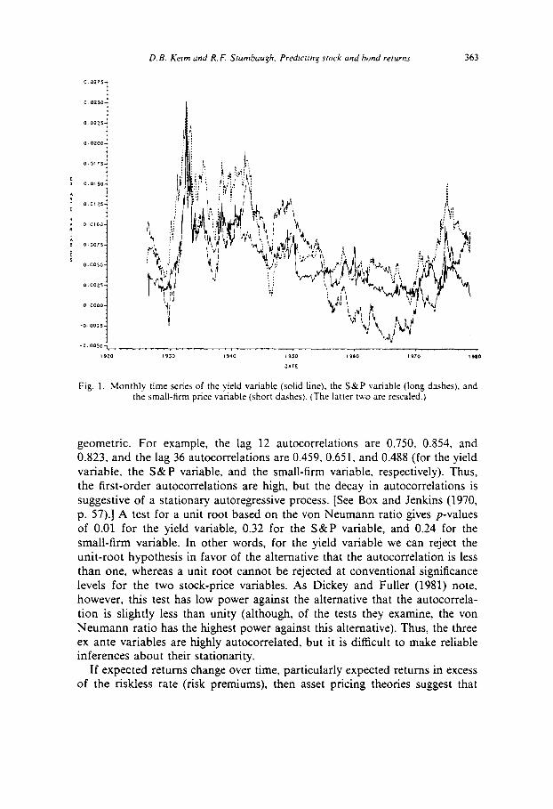
portfolio. Fig. 1 plots the monthly values of the three ex ante variables described
above. (The two stock-price variables are resealed in order to show all three series on the same graph.) The three series behave similarly, which suggests that one might view any of the three as proxying (inversely) for a general level of stock and bond prices.’ As the regressions that follow will demonstrate, all three series appear to be positively associated with expected future risk premiums.
The time series properties of the three ex ante variables are similar. The first-order autocorrelations are close to 1.0: 0.965 for the yield variable, 0.989 for the S&P variable, and 0.988 for the small-firm variable. The decline in higher-order autocorrelations is, for all three series, monotonic and nearly
‘Correlations between monthly levels range from 0.71 to 0.84; correlations between monthly first differences range from 0.34 to 0.75.
D. B. Kerm and R. F. Stumbuqh. Predtctrn; stock und bond returns 363
Fig. 1. ,Monthly time series of the yield variable (solid tine). the S&P variable (long dashes). and the small-firm price variable (short dashes). (The latter two are resealed.)
geometric. For example, the lag 12 autocorrelations are 0.750, 0.854, and 0.823, and the lag 36 autocorrelations are 0.459, 0.651, and 0.488 (for the yield variable, the S&P variable, and the small-firm variable, respectively). Thus, the first-order autocorrelations are high, but the decay in autocorrelations is suggestive of a stationary autoregressive process. [See Box and Jenkins (1970, p. 57).] A test for a unit root based on the von Neumann ratio gives p-values of 0.01 for the yield variable, 0.32 for the S&P variable, and 0.24 for the small-firm variable. In other words, for the yield variable we can reject the unit-root hypothesis in favor of the alternative that the autocorrelation is less than one, whereas a unit root cannot be rejected at conventional significance levels for the two stock-price variables. As Dickey and Fuller (1981) note, however, this test has low power against the alternative that the autocorrela- tion is slightly less than unity (although, of the tests they examine, the von Neumann ratio has the highest power against this alternative). Thus, the three ex ante variables are highly autocorrelated, but it is difficult to make reliable inferences about their stationarity.
If expected returns change over time, particularly expected returns in excess of the riskless rate (risk premiums), then asset pricing theories suggest that
364 D. B. Kelm und R. F. Stambaugh, Predrnng srock and bond returns
Fig. 2. Monthly time series of the standard deviation of the S&P.
these changes can be associated in part with changes in risk. Specific measures of risk vary across pricing models, but a simple measure is the variance of the return on the market portfolio. Merton (1980) entertains a model in which the expected risk premium on the market is proportional to market variance, and he uses the variance of the S&P as a proxy for market variance. Fig. 2 plots the monthly standard deviation of the S&P return, beginning January 1928, where the monthly standard deviation is the within-month standard deviation of daily returns.*
A comparison of figs. 1 and 2 suggests some positive association between the ex ante variables and the S&P standard deviation. For example, standard deviations were high and asset prices were low (the three ex ante variables were high) in the early 1930’s and again toward the end of that decade.’
*As in Merton (1980). the monthly variance is the sum of squared differences in log prices, where each squared difference is divided by the number of days between trades (to adjust for holidays and weekends).
‘Correlations between the standard deviation and the ex ante variables range from 0.41 to 0.63; first differences are correlated from 0.04 (the yield variable) to 0.32.
D. B. Kern and R. F. Srambaugh. Predmmg stock and bond returns 365
Leverage-related bankruptcy risks may also be inversely related to the level of stock prices, especially if the levels of nominal debt vary slowly through time. This study does not investigate the ability of specific risk measures to predict returns. lo Our basic obj ective. as motivated earlier. is to investigate whether expected returns vary with levels of asset prices. Nevertheless, one might reasonably argue that such variation in expected returns at least partially reflects changes in risk.
3. Predicting risk premiums with the ex ante variables
3. I. Risk premiums on long-term bonds and common stocks
We first examine risk premiums on seven portfolios formed from four bond and three stock categories that span a wide range of risk and return. The portfolios are:
LTGOV = long-term U.S. Government bonds; returns are compiled by Ibbotson and Sinquefield (1982) from the U.S. Government Bond File at the Center for Research in Security Prices (CRSP) at the University of Chicago;
LTCORP = high-grade long-term corporate bonds; returns are compiled by Ibbotson and Sinquefield (1982) from data supplied by Salomon Brothers (1946-1981) and Standard and Poor (19251945);
BAA = BAA-rated long-term corporate bonds; returns are compiled by Ibbotson (1979);
UBAA = under-BAA-rated long-term corporate bonds; returns are com- piled by Ibbotson (1979);
Q5 = common stocks making up the fifth quintile of firms ranked by size on the New York Stock Exchange (NYSE), i.e., the quintile containing the largest firms trading on the NYSE;”
Q3 = common stocks making up the third quintile of size on the NYSE;
Ql = common stocks making up the first quintile of size on the NYSE, i.e., the quintile containing the smallest firms trading on the NYSE.
‘oFrench, Schwert and Stambaugh (1985) investigate the ability of the S&P standard deviation to predict stock returns.
“Stock returns data are obtained from CRSP. To create quintiles, we rank in ascending order all NYSE firms on their market value of common equity (the product of price per share and number of shares outstanding) at the end of the previous year. Firms within a quintile are weighted. for a given month t, by placing equal weights on each stock at the beginning of month t - 1. The month r weights are then the second-month weights in a two-month buy-and-hold strategy. This reduces the bid-ask bias, as discussed by Blume and Stambaugh (1983).
366 D. B. Kern und R. F. Srumhuuyh, Predcrmg stock and bond r~wns
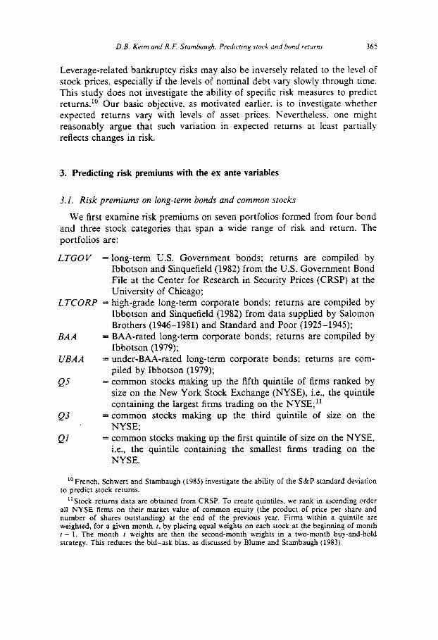
Data availability confines us to the period from January 1928 to November 1978.”
Table 1 presents summary statistics for the monthly risk premiums in the overall period and in two approximately equal subperiods. Risk premiums are computed for each portfolio as the difference between the monthly return on the portfolio and the monthly return on the shortest-term Treasury bill with at
least one month to maturity, as compiled by Ibbotson and Sinquefield (1982) from the CRSP U.S. Government Bond File. We list the assets by decreasing
grades for the bonds and then by decreasing firm size for the stocks. Both the averages and the standard deviations of the risk premiums (columns 1 and 2) tend to increase monotonically as one moves down the columns, although there are several exceptions. The correlations between premiums on different assets exhibit a similar property, in that as assets become farther apart on the scale, correlations decline. For example, the Government bonds have their highest correlation with the high-grade corporate bonds and then display progressively lower correlations with the lower-grade bonds and the stocks.
The risk-premium autocorrelations are in general significantly larger than zero
only at lags one and nine, and they are more pronounced for the lower-grade bonds and smaller stocks. The first-order autocorrelations could reflect non- synchronous trading [Fisher (1966)], or they could be one indication that expected premiums change over time.
We regress monthly risk premiums for each of the seven portfolios on the previous month-end value of each of the three ex ante variables: the yield variable ( yvsaA -_~~a), the S&P variable (-log SP/sp), and the small-firm variable (- log Pp,). The regressions are estimated using weighted least squares, where the weight used in each regression is the reciprocal of the within-month standard deviation of the daily S&P (displayed earlier in fig. 2). An investiga- tion of the residuals from the unweighted regressions reveals significant
heteroscedasticity, especially for the two lower-grade bond portfolios and the stock portfolios. In those cases, the heteroscedasticity test of White (1980) produces chi-square statistics well above conventional significance levels.
The S&P standard deviation provides a reasonably precise estimate of
within-month volatility, and it is used as a weight in all of the regressions under the assumption that volatilities on these seven long-term asset portfolios move together through time. In order to provide some empirical support for this assumption, we compute month-by-month estimates of standard devi- ations for each of the seven portfolios, where the estimate for a given month is based on returns for that month, the previous six months, and the following six months. For the two lower-grade bond portfolios and the three stock
“Most of our series begin in l/1926. but the regressions reported below use weighted least squares, and the weights (the S&P standard deviation) begin in l/1928. The low-grade bond series (BAA and below BAA) end in 11/1978.
x%l
,,I! ,I!
oJm
F!
UO
!l,?(.lJJ02Olfll?
.?nJl
J! p
O’() k(a
lew
!xoJd
dn
J0JJ.l
pJSp
u”IS,
W,.W
,S
aSA
N
ISJ(&S
JO a
lpu
!nb
=
10
!qm
s 3s~
~
JO a
lyu!n
b
alp
p!u
J =
fd
:s~
.mlS
~SA
N
lsa%
v[ JO
a[yu
!nb
=
sd
!((,&
I) u
oslo
qq
~
hq
p
alm
J1s~o
3 w
ap
u!
pu
oq
a
ieJo
d.u
oa
p
a!e
J-wg
-lap
on
=
yyg
fl !(6~
61) W
Sloq
qy
iq
pa
Km
Jrsuo
3 xa
pu
! p
uo
q
JleJO
dJO
3 p
ale
J-wg
=
yyg
!(Zg
(,I) p
laya
nb
u!S
pu
e
uo
sloq
q~
6q
p
al~
n~
lsuo
3 xa
po
! p
uo
q
a,e
Job
oa
ap
W%
q%
!q
wJJl-8U
O~
=
d
yoJd
7 !(Z861)
pla
yan
bm
s p
uE
uo
sloq
q~
6q
p
alJru
lSUO
~
Xa
pU
! p
uo
q
lua
mu
~a
~o
g
‘s’n
UK
+%
o[
-,fog~7 :m
sago%
)eJ pssv,
EZ
‘O
PO
’0 10’0
EO
’O-
01’0 E
O’O
E
UO
- P
O’0
WO
’O
ZO
’O-
80’0 - so’0
50’0 01’0
EI’O
- 11.0
10’0 PO
’0 60’0 -
LO
’0
PO0
IO.O- 60'0 OZ.0
EO'O- so'o-
ROO oz.0
ZO'O- so'o-
EOO SI'O
SO'0 ZO'O-
Kro 02'0
SO'O- to.0
11'0 oz.0
910 60'0-
PO'0 SO'0
SO'O- 60'0
10'0 zo'o
LO'0 00'0
80'0 91'0
wo- co‘o-
90'0 LI'O
IO'O- WYO- 10'0
El'0
LO.0 zo‘o-
wo 81'0
ZO'O- PO'0
11'0 81'0
80'0 Lo'0
LO'O- 11'0
MO- LO'0
90'0- 90'0
II’O-
II’O-
zo’o- 10’0
Il’O-
OI’O
- ZO
’O-
EO’O
EO’O
- RO
’O-
RO‘O
- so
’0
EO’O
- 80’0-
EO’O
w
’o-
LO’0
- EO
’O-
zo’o
01’0
IWO
- ZI’O
- zw
o-
zvo
00’0 -
60'0- IO'O- ZO'O--
wo
50’0 W
‘O-
90’0- 80’0
20.0 w
o- 10’0
60'0 ZO'O
20'0 LO'0
KJ'O 60'0
90'0 90'0
90'0 EO'O-
Lo'0 80'0
RO'O zo‘o
SO'O- 90‘0
ZI'O wo-
90'0- EO'O
zo’o 20.0
SO
’O-
WO
’O-
SW
0 w
o- S
O’O
- 10’0
90’0 00’0
W’O
- 90’0
EO
’O
LO’0
90’0 P
O.0
EO'O EO'O-
LO'0 60'0
EO'O LO'O-
zo'o- PO'0
PO'0 80'0-
IWO- 00'0
‘in’0 IW
O-
ZO
’O
01’0 LO'0
90‘0 10'0
91'0 E6'0
11'0 90'0
ZUO- 60'0
9L'0 26'0
01'0 so'0
10'0 Cl.0
OS0 IS0
IS0 W'O
ZI'O PI.0
PI'0 Et'0 IV'0 6E‘O
19'0 LO'0
ZO'O- EO'O-
El'0 62'0 IE'O 9CO
19'0 99'0
91'0 OI'O-
On'0 IWO--
11'0 SI'O IZ'O IPO
pp'n
XL61/11-CS61/1
OI'O- 60'0-
10'0 RI'0
LO'O- 9I'O-
10'0 RI'0
16'0 WO-
lZ'O- IO'O- PI'0
28'0 96'0
Zl.O- 91'0-
zo'o EZ'O
LL'O IR'O LL'O WO-
OZ'O- IWO-
9Z'0 29'0 69'0 L9.0
CR.0 80'0 90'0 + - LI'O
01'0 ZCO
62'0 tZ'0 09'0
LP'O OI'O-
20'0 EVO
SO'O- 50'0 SI'O 91'0
OC'O IV'0
zs6r/zl-sz6l/r
RO'O- LO'O-- 1
0'0
LI'O WO-
11'0- 10'0
81'0 16'0
CO'0 SI'O-
10‘0- El'0
18'0 G6'0
60'0- ZI'O-
ZO'O ZZ'O
EL'0 9L'0 ZL'O t'OO'O- EI
'O- 10'0
CZ'O
65'0 E9'0 19'0 6L'0
80'0 zo'o-
EO'O El'0
SZ'O 62'0 SZ'O wo
two
60'0
SO'O- ZO'O
ZO'O- 90'0 El'0 91'0
62'0 LE.0
8L61/11-8261/I
5590’0 PO
W0
SIWO
6LlO'O 6EIO'O SLIO'O
6L'0 RXIO'O
LSPI'O EIOI'O
06L0'0
81t'O'O L9Zo'O EOWO
EE'O
1210'0
6PII.O OOUO'O IEWO
ZZEO'O
EIZO'O
WIO'O
99'0 SSIO'O
p600’0 E900’0 000.0
E000’0 zm
o E000‘0- R
OO
O’O
-
L810'0 9110'0 6800'0
zmo LZWO 8ZlwO 1zoo'o
OVIO'O
6800'0 9900'0
zzoo'o SIOO'O
EIOO'O
LOOO'O
Id
:: vw
i v van
VV
8 dNOX7 AO3.17
spu
o,,
IO
:FT
w
w
v vm vvll
dtlOX7 AO3J7
vuoa
Id rc3 S
t3 S
?JolS
vvan V
W
d1102l7 /lo%!7
portfolios, the correlations between these ‘rolling’ standard deviations based on monthly data and the within-month standard deviation of the daily S&P range from 0.72 to 0.80. When, for those portfolios, White’s test is applied to the regressions weighted by the S&P standard deviation, the test statistics are considerably lower than in the unweighted regressions and are often less than conventional significance levels. For the long-term U.S. Government bonds and the high-grade corporate bonds, the correlations between the rolling standard deviations and the S&P standard deviation are 0.14 and 0.17, and White’s test gives similar results in both the weighted and unweighted regres- sions (homoscedasticity is rejected in the first subperiod but not in the second). In the case of those two portfolios, however, the coefficient estimates and standard errors are very similar for both the weighted and unweighted regressions, so we simply report the weighted regressions for all seven portfolios. We compute standard errors based on the heteroscedasticity-con- sistent method of White (1980) in order to allow for any heteroscedasticity remaining in the weighted regressions. l3
Table 2 reports for each regression the coefficient estimates, the t-statistics (based on the heteroscedasticity-consistent standard errors), the adjusted R-squared, and the first-order autocorrelation of the residuals. In the overall period, the estimated coefficients on all three ex ante variables are positive for all assets. The t-statistics on these coefficients range from 3.42 to 6.88 in the bond regressions and from 1.16 to 2.27 in the stock regressions. A test of whether the coefficients jointly equal zero across the seven portfolios gives F-statistics between 8.17 and 11.4 with 7 and 2086 degrees of freedom, thereby rejecting strongly equality to zero (these F-statistics are not adjusted for heteroscedasticity). Thus, the evidence appears to support the hypothesis that expected risk premiums change over time and that levels of asset prices contain information about expected premiums, especially for the bond port- folios.
The subperiod results, with a few exceptions, tend to confirm the results for the overall period. The F-test of joint equality to zero gives p-values less than 0.01 in both subperiods for all three ex ante variables. As in the overall period, the t-statistics are higher in the bond regressions. The t-statistics in the stock regressions are, in both subperiods, typically less than conventional signifi- cance levels, and the estimates themselves are sometimes negative in the second subperiod.
The weak results for the stock portfolio regressions in table 2 are somewhat misleading. As we show later in section 4, the predictive ability of these ex ante variables is seasonal, particularly for the low-grade bonds and the stocks of the medium-sized and small firms. When this seasonality is taken
“Hsieh (1983) recommends using the adjusted standard errors even when homoscedasticity is not rejected by White‘s test.
D.B. Keim and R. F. Stambaugh. Predicting sock and bond rerurns 369
Table 2
Regressions of monthly risk premiums on the ex ante variables.’
aRegressions are estimated using weighted least squares. The weight used in each equation is
l/%P. where asp is the within-month standard deviation of daily returns on the Standard and Poor’s Composite Index. The ex ante variables are defined as follows: ( Y,,aAA - YTB) = the difference between yields on long-term under-BAA-rated corporate bonds and short-term (ap- proximately one-month) U.S. Treasury bills; log(SP/p) = natural logarithm of the ratio of the real S&P Composite Index to its average value over the previous 45 years; - w = minus the natural logarithm of share price, averaged equally across the quintile of smallest market value on the NYSE.
bAsset categories are: LTGOY= long-term U.S. Government bond index constructed by Ibbotson and Sinquefield (1982); LTCORP = long-term high-grade corporate bond index con- structed by Ibbotson and Sinquetield (1982); BAA = BAA-rated corporate bond index con- structed by Ibbotson (1979); UBAA = under-BAA-rated corporate bond index constructed by Ibbotson (1979); QS = quintile of largest NYSE stocks; Q3 = middle quintile of NYSE stocks; Ql- quintile of smallest NYSE stocks.
‘R2 is the adjusted R-squared, and i,(u) is the first-order autocorrelation of the residuals (both statistics are based on the weighted residuals).
dHeteroscedasticity-consistent r-statistics in parentheses [White (1980)].
into account, the positive relation between the ex ante variables and ex post risk premiums becomes stronger.
The regressions reported in this study share a problem common to many empirical studies in finance and economics. The independent variable, al- though predetermined with respect to the dependent variable, is stochastic and most likely correlated with past regression disturbances. This phenomenon leads to finite-sample bias in the regression coefficients and the t-statistics, and the bias can be non-trivial even in samples of several hundred observations if the independent variable has both high autocorrelation and a high correlation with the past regression disturbances. In this application, where the correlation between the past regression disturbances and the independent variable is probably negative, the slope coefficient is biased upwards. The bias in the regressions reported in table 2 will be greatest when an asset’s own previous price level is used to predict that asset’s return (e.g., when the below-BAA return is regressed on the yield variable). When changes in the price-level variable are not highly correlated with the dependent variable, then the bias is
D. B. Kelm and R.F. Srambaugh, Predicrmg stock and bond returns 371
small (e.g., when the Government bonds are regressed on the small-firm variable). t4 Given the investigation reported in Stambaugh (1986) most of the r-statistics for the overall-period slope coefficients in table 2 still allow rejec- tion of equality to zero at conventional significance levels, particularly in the bond regressions. As noted, the weakest results occur in the stock regressions but the results to be discussed later indicate that the predictive ability in those regressions is strong in one month of the year (January). The latter result is not significantly affected by the bias described here.
When the regressions reported here are estimated instead using the same ex ante variables lagged several months, the results are very similar to those reported, with the explanatory power dropping gradually as the lags increase. We do not report the results of regressing risk premiums on two or more of the ex ante variables simultaneously. The variables are sufficiently collinear so that, in such regressions, no single variable produces reliably nonzero coeffi- cients.
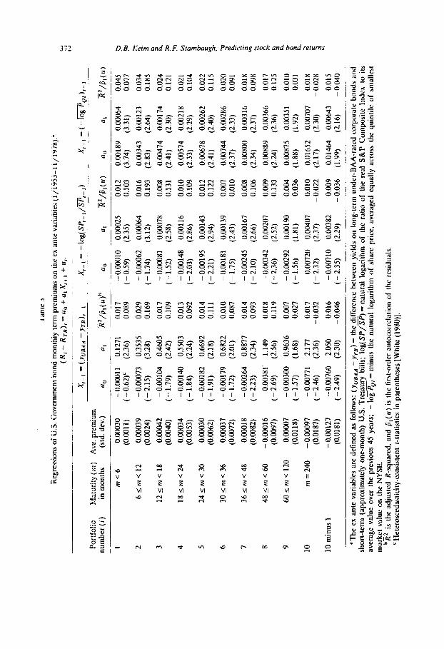
3.2, Term premiums on U.S. Government bona3
The previous section examines relatively long-lived assets whose future nominal payoffs possess different amounts of uncertainty. Table 2 begins with default-free Government bonds and then, roughly speaking, moves progres- sively through the spectrum of payoff uncertainty. We turn next to default-free instruments of different maturities. This section investigates whether the variables that predict risk premiums in the previous section also predict risk premiums, or ‘term premiums’, of U.S. Government bonds and notes with various maturities. Following Fama (1984) a term premium is defined as the difference between a bond’s return and the return on a one-month T-bill.
Our returns data consist of the file constructed by Fama (1984) from the CRSP U.S. Government Bond File. The file contains monthly returns, begin- ning in January 1953, on portfolios of notes and bonds (no bills) formed according to the ten maturity classifications listed in table 3 (second column). The first nine portfolios exclude ‘flower’ bonds with special estate tax features. The tenth portfolio is the same Ibbotson-Sinquefield portfolio used in the previous section. That portfolio contains the bond with maturity closest to twenty years, but the highest-priced (relative to par) flower bond is chosen when no ordinary bond of sufficient maturity exists.
We regress term premiums for each of the ten bond portfolios on the three ex ante variables described earlier. The regressions are estimated by ordinary least squares, and the t-statistics again reflect standard errors based on the
“Stambaugh (1986) investigates the bias when the independent variable obeys a first-order autoregressive process. He finds that the (absolute) bias increases with both the autocorrelation in the independent variable and the correlation of the regression disturbance with the innovation in the independent variable.
‘[(()R(,l) J,!q,+
,] sasaqluaJed U
! S
3!lS!lelS
-! lU
~lS~S
UO
~-~1~~~lSC
~J~SO
J~~~~ J
‘sp!np!ssJ arll JO
uo!ielaJJo.m
)ne J~P
JO-~S
J!I aq
l s!
(tl)ld
pm
‘pxenbs-y
paisnrpe 141 s! ,va
--. ‘aS
AN
“41
UO
an
ll?A
)Iq
JCW
lsa~[elus
JO alyu
!nb
aql
SS
OJ~!
Qlen
ba p
a%eJJA
e ‘m
!Jd a~eq
s JO
ru
ql!~c%
ol
IeJnleu
aq
l sn
u!w
=
ldd
801
- :ssear(
sp
snoyJd
aq) Ja~o an
p?,t a%~ar\c
sl! 01
xaplq ysodm
o3 ~
7~s
IFal aql
Jo
O!W
J aq
l JO
LU
qlpI?%O
l ~eJn
lnu
=
(dS
/dS
)%o
l !S
[[!q
h+ieaJ~
‘s.n
(qlU
om
-aUo
Q
lemptoJdde)
um
j+oqs
PU
I? S
pU
Oq
a1eJodJo.l p
W?
J-Vfr’Q
-JapU
n
UJJ&
%IO
[ U
O
“P&
i U
JlMlJq
32UaJ9.Jj~3q
l =
(LL
k -
“vsni)
:SM
OllO
J se
p3U
lJap
9Je S
a[ql?
!JVA
a)m
! X
3 Jq
Lr
Orn~
‘O -
<IO
’0
820’0 - R
IO’0
IlxO’O
010’0
SZ
I’O
LiO'O
R60'0 x 10’0
160’0 020’0
SII’O
Z
ZO
’O
tOI‘0
IZO
’O
IZI’O
bZ
O’0
SX
I’O
Pto’o
LLO'O SW0
("Wz2j
9E0’0 -
600’0
zzo’o - 010’0
9EO
’O
VO
O’O
EE
I’O
600’0
901’0 800’0
010’0 LOO.0
ZZI'O 210'0
601’0 O
IO’O
IEI’O
800’0
E61’0
910’0
EO
I’O
ZIO
’O
9W’O
- 910’0
ZE
O’O
- L
IO‘O
LZO'O LOO'0
611’0 8 10’0
E60’0
PIO
’O
L80'0 010'0
III’0 P
IO’O
260’0 E
IO’O
601’0 LIO'O
691'0 6ZO'O
680'0 LIO'O
(OC
Z’
(6p'Z-1 OSO'Z
09LOO'O-
;;g ILjg_)
cg;3 (a:;;'
(9s.z) (69'Z-)
6PI‘I .18EWO-
(PCZ) (EZ'Z-)
LL88'0 P9ZWO-
,;;g 6L;;:;-)
$;;:f z8;;:;I'
E(!g:;) OP~~:;~'
,$;:;' ,;;:;I'
,,'g;' tLg:x-)
(9E.Z) >(Z9.0--)
ILZI'O 11000'0-
(1810’0’ LZIOO'O-
(L810'0) L6000'0-
hrwo) Loooo'O
(L600.0) 9Iooo'O-
(zsOO.0) 81ooo'O
(ZLWO) LEOWO
(2900.0) OKKNO
wKs0) PEOWO
(OVOO'O) zpooo'o
(vzOO.0) 6fOOO'O
(IIWO
) O
tOO
O’0
opZ=
lU
I vu 01
01
OZ
I>'U
509 6
09 >'uF RP
8
8t7>'4'59E
9f.>m5 OE
OE >~~PZ
PZ
>“‘r81
8I>W5ZI
ZI>lU5:9
9 > lU
‘n (‘Q
P
‘PW
sq1uoul U
! _
(!) Jaqlu
nu
m
n!ru
aJd my
( tu) A
iynie~
o
![oJlJo
d
__~ I-‘(
‘Od
A-)
= ‘-‘x
(‘~‘d&
~‘d~)%
OI-
= ‘-‘Jf
lFl(f7.L~_ V
Vc
m~)=
1-J X
.‘n +
I+‘X
In+
On
=‘(81~
-!u
)
r’(8L6I/II-C
<6I/I)
sa\
qe
!JeA
alU
e X
J Jq
l U
O sru
nyaJd
UJJal
&U
O”
PU
Oq
,U
aUJU
JaAO
zof)
‘s’n
JO S
UO
!SS
aJ8+
c aae I
D. B. Kerm and R. F. Stambaugh, Predtcrtng srock and bond rcturru 373
heteroscedasticity-consistent adjustment of White (1980). Table 3 displays the results. The coefficient estimates on ail three variables are positive for all maturity classifications. and most are reliably non-zero. An F-test of whether the coefficients jointly equal zero gives p-values of 0.02 for the yield variable, 0.10 for the S&P variable, and 0.02 for the small-firm variable. These results
support the hypothesis that expected term premiums change over time. al- though the R-squared values are typically only one to two percent. Moreover,
the movements in expected term premiums are evidently associated with movements in the expected risk premiums on the other assets examined earlier. In other words, there appear to be common movements in expected returns for assets across a wide range of characteristics, and these movements
are reflected, in part, by levels of asset prices. The (unconditional) average premiums. also shown in table 3. are highest
for the third portfolio (12 to 18 months) and then decrease as maturities lengthen. This pattern of average premiums in the post-1953 period is noted
by Fama (1986), but. as Fama concludes, the average premiums are not reliably different across maturities. The variability of the longer-maturity bond returns makes it difficult to reject many hypotheses about the shape of the maturity structure of expected returns.
Both the intercept and slope coefficients in table 3 tend to vary monotoni- cally with maturity, unlike the average premiums, but here it is also difficult to reject equality of conditional expected premiums across portfolios, especially when the alternative hypothesis is vague or unspecified. An F-test for equality of the slopes and intercepts across the ten maturities gives a p-value of 0.06 for the yield-variable regressions, but the test gives much larger p-values for the other two ex ante variables. Similarly, testing for equality of only the slopes gives a p-value of 0.02 for the yield variable but larger p-values for the
other two variables. Somewhat stronger evidence against the null hypothesis of equality of
conditional expected premiums emerges when equality of the slope coefficients is tested against the alternative that the slope coefficients increase monotoni-
cally with maturity. If the ex ante variables proxy for a dimension of ex ante risk, then this alternative hypothesis essentially equates longer maturity to greater risk along that dimension. While one might argue that this is merely the alternative suggested by the data, we contend that it is also the alternative with the greatest a priori appeal. The simplest test suggested by this alternative is to compare the endpoints, i.e., the first and tenth portfolios. The last row of table 3 reports the results of regressing the difference in returns between the
tenth and first portfolios on the ex ante variables. The slope coefficients in all three regressions are reliably positive.
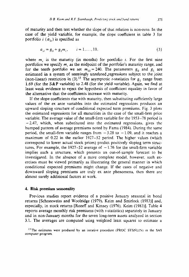
Another approach to testing equality against this more specific alternative. and one that uses all ten portfolios, is to specify the regression slope coeffi- cients as a function of maturity. We model the coefficients as a linear function
374
0.019
0.001
-0.008 10
4.60 MA TlJRITY
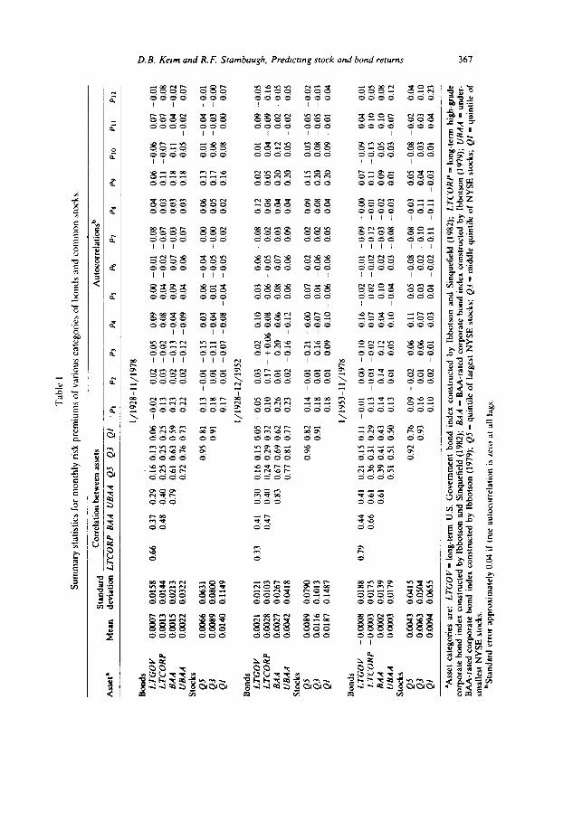
Fig. 3. Fitted regressions of term premiums ( PREXIILrM) on the small-firm (PRICEVAR) for each of ten maturity classifications (MATURITY).
price variable
of maturity and then test whether the slope of that relation is non-zero. In the case of the yield variable, for example, the slope coefficient in table 3 for portfolio i (a,,) is specified as
a,, = go + g1m, 7 i=l ,..., 10.
where m, is the maturity (in months) for portfolio i. For the first nine portfolios we specify m, as the midpoint of the portfolio’s maturity range, and for the tenth portfolio we set m,, = 240. The parameters g, and g, are estimated in a system of seemingly unrelated,regressions subject to the joint (non-linear) restriction in (3). i5 The asymptotic t-statistics for g, range from 1.69 (for the S&P variable) to 2.48 (for the yield variable). Again, we find at least weak evidence to reject the hypothesis of coefficient equality in favor of the alternative that the coefficients increase with maturity.
If the slope coefficients rise with maturity. then substituting sufficiently large values of the ex ante variables into the estimated regressions produces an upward sloping structure of conditional expected term premiums. Fig. 3 plots the estimated regressions for all maturities in the case of the small-firm price variable. The average value of the small-firm variable for the 1953-78 period is - 2.47, which, when substituted into the estimated regressions, gives the humped pattern of average premiums noted by Fama (1984). During the same period, the small-firm variable ranges from - 3.28 to - 1.09. and it reaches a maximum of 0.22 in the earlier 1927-52 period. The higher values (which correspond to lower actual stock prices) predict positively sloping term struc- tures. For example, the 1927-52 average of -1.76 for the small-firm variable implies such a structure, which presents an out-of-sample forecast to be investigated. In the absence of a more complete model, however, such ex- ercises must be viewed primarily as illustrating the general manner in which conditional expected premiums might change. If the cases of negative and downward sloping premiums are truly ex ante phenomena. then there are almost surely additional factors at work.
4. Risk premium seasonality
Previous studies report evidence of a positive January seasonal in bond returns [Schneeweiss and Woolridge (1979). Keim and Smirlock (1983)] and, especially, in stock returns [Rozeff and Kinney (1976). Keim (1983)]. Table 4 reports average monthly risk premiums (with t-statistics) separately in January and in non-January months for the seven long-term assets analyzed in section 3.1. The averages are computed using weighted least squares to estimate a
‘5Tbe estimates were produced by an iterative procedure (PROC SYSSLIN) in the SAS computer program.
316 D. B. Keim and R. F. Smmbaugh. Predicrmg sock and bond returns
D. B. Ketm and R. F. Srambaugh. Predrnng srock and bond returns 377
regression of risk premiums on two dummy variables. The weights used in each regression are l/asp. the reciprocal of the within-month standard devia- tion of the S&P. The r-statistics are again based on the White (1980) adjusted standard errors.
We find in table 4 the same January seasonality in risk premiums on many assets. With the exception of the long-term government bonds and the largest common stocks, mean risk premiums are significantly larger in January than in non-January months. l6 Further the difference in means is more pronounced for lower-quality bonds and smaller stocks. The F-statistic in column 4 for each period tests the hypothesis that monthly expected risk premiums are equal in non-January months; we can reject equality only for the below-BAA bonds, primarily due to the first subperiod.
That this seasonality has occurred consistently for more than fifty years suggests that it relates to an ex ante phenomenon. In this section we report a January seasonal in the estimated regression coefficients for our ex ante variables.
4. I. Seasonality and the risk premium regressions
We regress risk premiums on the ex ante variables and estimate the coefficients separately in January and in non-January months (again using weighted least squares). Although the coefficients on all three ex ante variables exhibit similar seasonality, the seasonal pattern is strongest for the coefficients on the small-firm price variable. In the interest of brevity, we report only the small-firm variable regressions for the remainder of the paper.
Table 5 reports the regression results for the overall period and for both subperiods. In the overall period, the coe.%ients on the small-firm variable are generally positive in January and in non-January months (the only negative coefficient is the January coefficient for high-grade corporate bonds). and the January coefficients are larger than the non-January coefficients (with the exception of government and high-grade corporate bonds). The non-January coefficients are significantly non-zero for the bond portfolios but not for the stock portfolios (the t-statistics are 4.18 or more for the bonds but 1.56 or less for the stocks). The January coefficients are significantly non-zero for the lower-grade bonds (BAA and below-BAA) and all but the largest stocks. The coefficients on the small-firm variable tend to increase with decreasing grade for the bonds and with decreasing size for the stocks, but this pattern is more pronounced for the January coefficients. As a result, the t-statistic of the differences between the January and non-January coefficients, t(a,, - a,,),
16The r-statistic t(a, - aI) in the third column of each period’s results tests the LqTothesis that the difference in means is zero. In the overall period, the f-statistics for LTCORP, BAA, UBAA, Q3 and QI have p-values less than 0.05.
378 D. B. Keim and RF. Stambaugh, Predicting stock and bond returns
Table 5
Regressions of monthly risk premiums on the small-firm price variable in January and in non-January monthsa
“Regressions are estimated using weighted least squares. The weights used in each equation are l/asp, where asp is the within-month standard deviation of daily returns on the Standard and Poor’s Composite Index. The sma.ll-tirm price variable. - log PQ,, is minus the natural logarithm
of share price. averaged equally across the quintile of smallest market value on the NYSE. The dummy variable d,, is defined as d,, = 1 if month t is a January; d , = 0 otherwise.
‘Asset categories are: LTGOV= long-term U.S. Government Land index constructed by Ibbotson and Sinquefield (1982); LTCORP = long-term high-grade corporate bond index con- structed by Ibbotson and Sinquefield (1982): BAA = BAA-rated corporate bond index con- structed by Ibbotson (1979); UBAA = under-BAA-rated corporate bond index constructed by Ibbotson (1979); Qj = quintile of largest NYSE stocks; Q3 = middle quintile of NYSE stocks: QI = quintile of smallest NYSE stocks.
’ Heteroscedasticity-consistent r-statistics in parentheses [White (198O)l. dRZ is the adjusted R-squared based on the weighted residuals. ‘j,(u) is the first-order autocorrelation of the weighted residuals.
tends to increase as one moves down the column, and equality of the coefficients is rejected for the lowest-grade bonds and the smallest stocks. The effects discussed above are found in both subperiods.
4.2. Seasonality and differences in returns between assets of the same type
Much of the literature on seasonality in stock returns focuses on seasonality in the so-called ‘size effect’, defined as the difference in common stock return between the smallest and the largest firms [e.g., Keim (1983)]. The evidence in table 4 suggests that a similar seasonal exists in the difference in returns between low-quality bonds (e.g., U&IA) and high-quality bonds (e.g., LTGOV). We regress differences in returns from the bond market ( RUBA A - R LTcov) and the stock market (R,, - Ros) on the small-firm price variable. Panel A of table 6 reports the results for the bond returns and panel B contains the results for the stock returns.
The coefficients on the small-firm variable in the overall period are, for both the bonds and the stocks, reliably positive in January (both t-statistics are
380 D. B. Keim and R. F. Stambaugh, Predicrmg stock and bond returns
approximately 3.5). but the non-January coefficients are not significantly greater than zero. Further, the January coefficient is significantly larger than the non-January coefficient in both regressions. The same results appear in both subperiods, although the effects are weak for the bonds in the second subperiod.
The regressions in table 6. particularly those in panel B. demonstrate that the small-firm price variable and the January intercept dummy explain a substantial portion of the variation in the return differences. For example, these regressions explain 23% of the variation in the difference in monthly stock returns between the smallest and largest firms over the 1928-78 period and 27% in the 1953-78 subperiod. The explanatory power of the small-firm price variable when the regressions are computed in January only is also quite high. For example, the January R* for the stocks is 32% for the total period and 36% for the early subperiod.
4.3. The prospect of seasonal risk
As the regressions reported above indicate, returns on all assets tend to be highest when stock prices are low, but this tendency is concentrated in January for many of the assets, especially stocks of small firms and low-grade bonds:If low stock prices serve as a rough measure of increased risk of some sort. then this seasonality in regression coefficients suop DOests that the risk accompanying a given level of stock prices tends to be highest around the turn of the year.”
Estimates of the traditional risk measure, beta, display some seasonality. For example, using daily stock returns on firms in the lowest twentieth of all NYSE and AMEX firms ranked by size, Rogalski and Tinic (1984) report (unconditional) OLS beta estimates of 1.34 in January as compared to 1.01 in the next highest months (February and December). To explain the seasonality in average returns using the traditional asset pricing theory, however. such relatively small changes in beta require an implausibly high market risk premium.
Examining unconditional betas may not be entirely appropriate, however, given that most pricing models call for conditional moments rather than
“Low prices might also indicate previous tax losses, thereby supporting the hypothesis that the January returns reflect a rebound from tax-loss selling pressure. Roll (1983) finds that returns on an equally-weighted stock index in the preceding year are negatively correlated with returns surrounding the turn of the year, and he suggests a tax-loss selling explanation for these results. We do not attempt to rule out such an explanation. Rather, we simply suggest an alternative, perhaps additional, source of the observed phenomenon. Reinganum (1983, p. 102) concludes that ‘potential tax-loss selhng does not seem capable of explaming the entire anomalous return behavior of small firms in January’. Chan (1985) finds that, cross-sectionally, returns in a given year are negatively correlated with January returns two years hence, and he also concludes that tax selling cannot be the sole explanation of the observed seasonality.
382 D. B. Kelm and R. F. Srambaugh. Predicrlng stock and bond renm.s
unconditional moments. For example, conditionai covariances between pre- whitened series, rather than unconditional covariances, are generally the relevant risk measures (Blk’s) in models as in (1).18 The ex ante variables used here are candidates for prewhitening many return series to obtain deviations from conditional means. For many assets, where the explanatory power of the regressions is relatively low, the distinction between conditional and uncondi- tional cross-sectional risk measures may be minor. For other assets, however, where the explanatory power is higher, e.g.. January returns on small-firm stocks and low-grade bonds, the distinction may prove to be important.
We first examine the unconditional and conditional market betas of the return difference between the small-firm portfolio (Q!) and the large-firm portfolio (QS). The conditional betas are computed by prewhitening this return difference as well as the value-weighted NYSE return using the small- firm price variable (i.e., using regressions as reported in tables 5 and 6). Betas are estimated separately for January and for February through December. As might be expected given the low explanatory power of the prewhitening regressions in February through December, the February-December condi- tional betas are not substantially different from the February-December unconditional betas in either subperiod. In the first subperiod, the January conditional beta estimates are not substantially different from the January unconditional estimates. In the second subperiod, however, the January condi- tional estimate is smaller than the unconditional estimate, 0.34 versus 0.71. Further, unlike the unconditional estimates in that subperiod, the conditional January beta is no longer significantly larger than its February-December counterpart (the t-statistic for the difference is 1.58). These results suggest that the distinction between conditional and unconditional market betas could be important in January, but the fact that the conditional betas display even less seasonality than the unconditional estimates offers little additional insight into the seasonality in mean returns.
We next examine seasonality in both conditional and unconditional esti- mates of a risk measure that Chan, Chen and Hsieh (1985) argue plays a key role in explaining the average return difference between small and large firms. The risk measure is obtained by regressing an asset’s return on the spread in returns between low-grade corporate bonds and U.S. Government bonds (‘PREM’). This ‘PREM beta’ is estimated in a multiple regression, and the value-weighted NYSE return is used here as the other independent variable. As in the case of the simple market betas above, the conditional estimates are obtained by first prewhitening all return series using the small-firm price variable.
“Two exceptions, in which unconditional covariances are appropriate even if there exist ex ante variables with predictive ability, are the models in Grossman and Shiller (1982) and Stambaugh (1983).
D. B. Kelm und R. F. Srumhuuqh. Predlcrlng rrock and bond rerurns 383
For the 1953-78 subperiod. w&h corresponds roughly to the period examined by Chan, Chen and Hsieh, we compute PREM betas for the difference in returns between the small-firm portfolio (QI ) and the large-firm portfolio (Q5). In February through December, both the conditional and unconditional PREM betas are positive and nearly identical. In January, however, the estimated conditional PREM beta of the return difference is significantly negative (t = -2.12) and significantly less than the February- December value (t = - 2.48). The same seasonality appears in the uncondi- tional estimates, but the January value is neither significantly negative (t = - 0.63) nor significantly less than the February-December value (t = - 1.02). Thus, again it appears that the distinction between conditional and uncondi- tional risk measures can be important in January.
A more striking outcome of the last exercise, however, is the negative January seasonal in the PREM betas. In fact, when the equally-weighted NYSE index is used instead of the value-weighted index, both the conditional and unconditional January PRElM betas are significantly negative (f = - 3.01 and t = - 2.24) and significantly less than the February-December estimates (t = - 3.08 and t = -2.35).i9 Given that the estimated PREM betas of large firms exceed those of small firms in January, it becomes difficult to use these estimated risk measures to explain the size effect in that month, which is when most of the total size effect has occurred. It appears at least that seasonality in the PREM betas, if present, does not correspond to the seasonality found in the size effect.20
The results above indicate some seasonality in covariance-based risk mea- sures, but, based on conditional estimates of those measures, the seasonality is either weak (for the market beta) or opposite to the seasonal in mean returns (for the PREM beta). An alternative approach is to investigate the presence of seasonality in a less traditional risk measure - one not based on covariances. We test for seasonality in the ex ante one-month default premiums on private-issuer instruments examined by Fama (1986). Default premiums are defined as returns in excess of identical-maturity T-bills. Average default premiums on the private-issuer instruments are highest in January. For exam- ple, the average default premium on Al-P1 commercial paper for the period
“The r-statistics reported here and in the previous paragraph are obtained from regressions that include observations for all twelve months but where the coefficients (including the intercepts) are allowed to differ in January. In other words, the estimated residual variance used in computing standard errors is based on data from all twelve months. When the r-statistics for the January values are computed using only January data, the January values are not reliably negative.
“The seasonality found here in the standard regression-based PRElM betas using the bond return spread is not necessarily found in other versions of this type of risk measure. For example, Nai-fu Chen informs us that this seasonahty does not appear in estimates where the means used in computing the January regression coefficients are based on twelve-month values rather than January values (i.e., where the twelve-month means are subtracted from the January values and the regression is then computed in January without an intercept).
384 D. B. Keim and R. F. Stambaugh Predicting stock and bond returns
l/1967 to 2/1984 is 1.17% (annualized) over all months, but January’s average (annualized) premium of 1.74% is the highest of all months. To test more formally for seasonality, we estimate the time series regression
0.359 0.695 0.640 (4.41) (3.84) (12.14)
R= = 0.44, 6,(U) = -0.12,
where R,, is the annualized percent return for one-month commercial paper, R TB is the annualized percent return on a one-month T-bill, and d,, = 1 if month t is a January (zero otherwise). Results for all of the private-issuer instruments are sufficiently similar so that results are reported for commercial paper only. The t-statistic of 3.84 on the January dummy indicates that investors in one-month instruments receive, other things equal, a significantly larger default premium in January. Given the apparent liquidity of these instruments, it is difficult to attribute these premiums to anything other than the probability of default. This result suggests that, if these instruments are priced rationally, the perceived ex ante risk of rare bad news (defaults) varies seasonally.
In light of these findings, we may wish to reconsider the regression results reported in tables 5 and 6. As argued previously, the results in those tables are consistent with the hypothesis that conditional expected returns and risk are higher (i) in January and (ii) in years when stock prices are low. However, if the appropriate measure of risk includes the possibility of rare bad-news outcomes, then the ex post sample results will tend to overstate the expected returns whenever the bad-news whose risk was perceived was not realized ex post. Thus, even though the expected returns might indeed vary in the manner suggested by the regressions, one should probably be cautious in viewing the total magnitudes as ex ante quantities. To illustrate this possibility, imagine that the probability of a lit-m’s announcing very bad news drops following the turn of the year. For example, if the probability of bad news, conditional on no announcement, takes a discrete drop at year end, then the stock price takes a .iiscrete jump upward. 21 This gives a large return to holding
21We briefly describe here some evidence that at least weakly supports the hypothesis that the probability of very bad news drops following the turn of the year, especially for small firms. During the 1927-81 period, delistings of small firms (lowest quintile) were most frequent during December (30 delistings) and least frequent in January (18 delistings), and delistings of smah firms were accompanied by average monthly returns of - 19.2%. These delistings are those for which there was no notice of delisting prior to the given month, as classified by CRSP. Roll (1983) also observes that delistings occur more frequently near January 1. In addition, during the 1926-82 period, individual smaJMrm returns less than - 50% were most frequent in December and returns less than -40% were least frequent in January. (We exclude a firm’s return in the month of delisting.)
rhe stock over the turn of the year. Moreover. this return Lvill be largest in years of greatest ex ante risk (or perhaps lowest stock prices).
5. Forecasting risk premiums with the small-firm price variable
The previous sections demonstrate that the small-firm price variable receives positive and significant coefficients in regressions with a wide array of asset returns. As a further check on the validity of these estimated regressions, this section investigates the ability of the regressions to make out-of-sample forecasts. Such an exercise, in addition to providing a somewhat more practi- cal perspective, allows us to verify that the bias discussed earlier in section 3.1 does not significantly influence the reported regression results. An evaluation
of forecasting ability outside our sample period would permit an analysis of
only five or six years of data (when available). An alternative that allows for
comparisons over a much longer period is to use 1928 through 1952 as our initial base period and to examine forecasts over the 1953-1978 period. We compute ‘one-step-ahead’ forecasts. which are based on parameters estimated using data for all periods up to but not including the forecast period.
Our objective is to compute one-step-ahead forecasts of risk premiums based on regression parameters estimated with the small-firm price variable and then to compare these with ‘naive’ forecasts of risk premiums based on their historical means. Table 7 reports the percentage reduction in mean square forecast errors obtained from comparisons of regression and naive forecasts. As a rough measure of the statistical significance of the improve- ment in forecasting ability, we report a t-statistic that tests whether, across forecasts, the sum of the forecast errors is correlated with the difference between the errors. This test is equivalent to a test of equality of mean square forecast errors under the assumptions that the individual forecasts are unbi- ased and the forecast errors are not autocorrelated [see, e.g., Granger and Newbold (1977)].**
The results for the one-month-ahead forecasts are reported in table 7. Mean square forecast errors are computed over all months as well as separately for January and February-December in order to examine seasonal patterns in forecasting ability. We define the percentage reduction in MSE for one- month-ahead forecasts as 100 x (MSE, - MSE,)/M.SE,, where MSE, is the MSE of the one-month-ahead forecast based on the regression
ASSET - RT,), = %_&, + ‘,r(’ - $) + ‘,,
22 The r-statistic is ‘rough’ in the sense that, if the true forecasting ability bf our regression model is zero, then the variance of the forecast errors from the naive model is less than the variance of our regression forecast errors. due to the extra noise that results from estimation of additional parameters in the latter model. Thus. the expected value of the r-statistic reported here is negative with no forecasting ability. Finding r-statistics equal to zero is actually mild evidence of some predictive ability.
386 D. B Keim and R. F. Srambaugh, Predicting stock and bond refurm
Table 7
Performance of one-month-ahead forecasts based on the small-firm price variable (1953-1978).
Asseta
Percentage reduction in mean square errorb (t-statistic in parentheses)
All Jan. Feb.-Dec. months
Bonds
LTGOV
LTCORP
BAA
I/BAA
UBAA-LTGOV
Stocks
- 1.92 2.68 2.24 ( - 0.52)C (1.33) (1.20)
- 2.98 3.81 3.11 ( - 0.57) (2.09) (1.80)
11.50 2.19 3.53 (0.86) (1.09) (1.53)
33.93 -4.19 0.64 (1.64) (- 1.39) (0.18)
28.15 - 7.53 - 4.94 (1.24) (- 2.55) (- 1.46)
QS 10.84 - 6.28 - 3.73. (1.98) (- 2.75) (- 1.75)
Q3 16.16 - 6.41 - 2.02 (2.69) ( - 2.99) ( - 0.98)
Q1 41.85 - 6.75 7.78 (2.69) (- 3.39) (2.28)
Ql-Q5 40.54 - 1.84 13.07 (1.86) (- 1.39) (2.93)
‘Asset categories are: LTGOV= long-term U.S. Government bond index constructed by Ibbotson and Sinquefield (1982); LTCORP = long-term high-grade corporate bond index con- structed by Ibbotson and Sinquefield (1982); BAA = BAA-rated corporate bond index con- structed by Ibbotson (1979); C/BAA = under-BAA-rated corporate bond index constructed by Ibbotson (1979); QS = quintile of largest NYSE stocks; Q3 = middle quintile of NYSE stocks: Qf = quintile of smallest NYSE stocks.
bThe upper value is 100 X (MSE, - MSE,)/MSE,, where MSE, is the mean square error of one-step-ahead forecasts based on the regression
0 ASSET -h),=u d,, + a,,(1 - d,,) + C.
and MSE, is based on the regression (estimated with WLS)
(a ASSET -RT~)r=a~,~r+a~,(l-~r)+a~,d,r(=log),_,
+a,,(1 -d,,)(-log),-l + K.
where q is the natural logarithm of share price averaged equally across the quintile of the smallest NYSE firms. d , = 1 if month r is January; d,, sets of forecasts begins i/1928.
= 0 otherwise. The base period for both
‘The r-statistic tests whether, across forecasts, the sum of the forecast errors is correlated with the difference between the errors. The true correlation is zero if both series produce unbiased errors with the same variances. This test is equivalent to a test of equality of mean square forecast errors; see, e.g., Granger and Newbold (1977).
D. B. Kerm and R. F. Slambaugh. Predicrrng rlock and bond re~urnx 387
and MSE, is based on the regression (estimated with WLS)
P ASSET -RT~)r=ao,d,,+a,,(l-d,,)+n,,d,,(-logPei),-,
(6)
where d,, is a January dummy. Thus our naive forecasting model, represented by eq. (5), accounts for the seasonal variation in the (unconditional) mean of past returns, while the model of eq. (6) also accounts for seasonal variation in conditional mean returns given the level of small-firm prices. We report results for our seven asset categories as well as for the return differences discussed in section 4.2.
The results for the one-month-ahead forecasts show that, for the stocks and for the lower-grade bonds, most of the improvement in forecasting ability using eq. (6) arises from the January forecasts. Thus, these results support the regression estimates reported in section 4. The improvement in January ranges from an 11% reduction in MSE for large-firm stocks to 42% for small-firm stocks. The r-statistics for the three stock portfolios indicate statistically reliable reductions in MSE. In February-December, however, the naive forecast for the lowest-grade bonds and all three stock portfolios outperforms the forecast based on eq. (6). A similar pattern is observed for differences in returns of similar assets: the improvements in January forecasting ability are 28% for UBAA minus LTGOV and 41% for Ql minus QS. For the long-term government and high-grade corporate bonds, on the other hand, forecasting ability is not concentrated in January. Overall, the results suggest that the forecasting model in eq. (6) possesses predictive ability for a wide array of asset returns.
6. Implications for future research
The fundamental conclusion to be drawn from this study is that expected risk premiums on many assets appear to change over time in a manner that is at least partially described by variables that reflect levels of asset prices. This paper’s results suggest several directions for future research.
If expected risk premiums or discount rates change, then one asset’s price relative to others is determined in part by the covariance between unantic- ipated returns on that asset and unanticipated changes in expected risk premiums. Chen, Roll and Ross (1983) in a test of such a cross-sectional pricing relation, propose a bond return spread (described earlier) as a proxy for changes in expected risk premiums. This study’s evidence suggests that such a variable is indeed likely to proxy for changes in expected risk premiums on many assets. If relative bond prices, say as summarized by the yield spread
388 D. B. Kerm and R. F. Stumbaugh, Predictrng stock and bond returns
used in this study, contain ex ante information about expected risk premiums, as our evidence indicates, then a change in relative bond prices, or a return difference, is likely to contain ex post information about changes in expected premiums. By the same reasoning, our evidence that levels of stock prices also contain information about expected risk premiums suggests that stock returns also contain information about changes in expected premiums.
Section 4.3 discussed using the ex ante variables to obtain conditional risk measures. In addition to conditional risk measures, conditional means them- selves may allow more precise inferences about various hypotheses. For example, the evidence on term premiums discussed in section 3.2 indicates that the relation between conditional expected bond returns and time to maturity varies through time. The difference in conditional expected return between long-term and short-term bonds appears to vary inversely with asset price levels. Conditional on sufficiently low asset prices, or perhaps sufficiently high risk, the estimated regressions suggest that the term structure of expected returns slopes upward. If true, such behavior could make unconditional averages of term premiums less useful in making inferences about the shape of the term structure.
One question that arises naturally in a study such as this is whether additional ex ante variables have predictive ability. We have chosen to define this study by restricting the number of ex ante variables and examining risk premiums on a wide spectrum of assets, but the investigation could be extended across a range of ex ante variables as well. A possible approach would be to decompose our variables into several components. For example, the single yield spread could be replaced by a number of yield spreads between instruments of various default risks and maturities.
Finally, we conclude that seasonality must be a consideration of any study dealing with changing expectations. Not only is seasonality present in average risk premiums on many assets, conditioned on simply the month of the year, but seasonality is found also in the regression coefficients on the ex ante variables that appear to predict risk premiums.
References
Blume. Marshall E. and Robert F. Stambaugh, 1983, Biases in computed returns: An application to the size effect. Journal of Financial Economics 12, 387-404.
Bodie, Zvi. 1976. Common stocks as a hedge against inflation. Journal of Finance 31. 459-470. Box. George E.P. and Gwilym M. Jenkins, 1970. Time series analysis: Forecasting and control
(Holden-Day, San Francisco, CA). Breeden, Douglas T., 1979. An intertemporal asset pricing model with stochastic consumption and
investment opportunities, Journal of Financial Economics 7, 265-296. Campbell, John Y., 1984, Stock returns and the term Structure, Unpublished working paper (Yale
University, New Haven. CT). Chan, K.C.. 1985, Can tax-loss selling explain the January seasonal in stock returns?, Unpublished
working paper (Ohio State University, Columbus, OH).
D. B. Keinr md R. F. Srmbaugh. Predmzg sack and bond returns 389
Chart. K.C.. Nai-fu Chen and David Hsieh, 1985, An exploratory investigation of the firm size effect, Journal of Financial Economics 14,451-471.
Chen. Nai-fu, Richard Roll and Stephen A. Ross, 1983, Economic forces and the stock market: Testing the APT and alternative aSset pricing theories. Unpublished working paper (University of Chicago, Chicago, IL).
COX. John C., Jonathan E. Ingersoll and Stephen A. Ross, 1985. An intertemporal general equilibrium model of asset prices, Econometrica 53, 363-384.
Dickey, David A. and Wayne A. Fuller. 1981, Likelihood ratio statistics for autoregressive time series with a unit root, Economettica 49, 1057-1072.
Fama. Eugene F., 1977. Risk-adJusted discount rates and capital budgeting under uncertainty, Journal of Financial Economics 5, 3-24.
Fama. Eugene F., 1981, Stock returns, real activity, inflation, and money, American Economic Review 71, 545-565.
Farna. Eugene F., 1984. Term premiums in bond returns. Journal of Financial Economics 13. 529-546.
Fama, Eugene F., 1986, Term premiums and default premiums in money markets, Journal of Financial Economics 17, forthcoming.
Fama, Eugene F. and G. William Schwert, 1977, Asset returns and inflation, Journal of Financial Economics 5. 115-146.
Fisher. Lawrence, 1966, Some new stock market indices, Journal of Business 49, 191-225. French, Kenneth R., G. William Schwert and Robert F. Stambaugh, 1985, Expected stock returns
and volatility, Unpublished working paper (University of Chicago. Chicago, IL). Gibbons, Michael R. and Wayne Ferson, 1985, Testing asset pricing models with changing
expectations and an unobservable market portfolio, Journal of Financial Economics 14, 217-236.
Granger, C.W.J. and Paul Newbold, 1977, Forecasting economic time series (Academic Press. New York).
Grossman, Sanford J. and Robert J. Shiller, 1981. The determinants of the variability of stock market prices, American Economic Review 71. 222-227.
Grossman, Sanford J. and Robert J. Shiller, 1982, Consumption correlatedness and risk measure- ment in economies with non-traded assets and heterogeneous information. Journal of Finan- cial Economics 10, 195-210.
Hansen, Lars P. and Kenneth J. Singleton, 1983, Stochastic consumption, risk aversion. and the temporal behavior of asset returns, Journal of Political Economy 91. 249-265.
Hsieh. David A., 1983, A heteroscedasticity-consistent covariance matrix estimator for time series regressions, Journal of Econometrics 22, 281- 290.
Ibbotson. Roger G.. 1979. The cornorate bond market: structure and returns. Unuublished working paper (University of Chicago, Chicago, IL).
Ibbotson, Roger G. and Rex A. Sinquefield, 1976, Stocks. bonds, bills, and inflation: Year-by-year historical returns (1926-1974). Journal of Business 49, 11-47.
Ibbotson, Roger G. and Rex A. Sinquefield, 1982, Stocks, bonds, bills and inflation: The past and the future (Financial Analysis Research Foundation. Charlottesville, VA).
Jaffe, Jeffrey F. and Gershon Mandelker, 1976, The Fisher effect for risky assets: An empirical investigation, Journal of Finance 31. 447-458.
Keim, Donald B., 1983, Size-related anomalies and stock return seasonality: Further empirical evidence, Journal of Financial Economics 12. 13-32.
Keim, Donald B. and Michael Smirlock. 1983. Bond returns, firm size and abnormal January returns, Unpublished working paper (University of Pennsylvania. Philadelphia. PA).
Kleidon, Allan W., 1983. Stock prices as rational forecasters of future cash flows, Ph.D. dissertation (University of Chicago, Chicago, IL).
Leroy, Stephen F. and Richard D. Porter, 1981, The present-value relation: Tests based on implied variance bounds. Econometrica 49. 555-574.
Lintner, John, 1965, The valuation of risk assets and the selection of risky investments in stock portfolios and capital budgets, Review of Economics and Statistics 47, 13-37.
Long, John B., 1974. Stock prices, inflation, and the term structure of interest rates, Journal of Financial Economics 1, 131-170.
Lucas. Robert E.. 1978, Asset prices in an exchange economy, Econometrica 46, 1429-1446.
390 D. B. Ktwn and R.F. Stambaugh. Predicrrng stock and bond returns
Merton. Robert C., 1973, An intertemporal capital asset pricing model, Econometrica 41, 867-887.
Merton, Robert C., 1980, On estimating the expected return on the market: An exploratory investigation, Journal of Fiiancial Economics 8, 323-361.
Miller, Merton H. and Myron S. Scholes, 1982, Dividends and taxes: Some empirical evidence, Journal of Political Economy 90,1118-1141.
Nelson. Charles R.. 1976. Inflation and rates of return on common stock. Journal of Finance 31. 471-483.
Reinganum, Marc R., 1983, The anomalous stock market behavior of small firms in January, Journal of Financial Economics 12, 89-104.
Rogalski, Richard J. and Seha M. Tinic, 1984, The January sixe effect: Anomaly or risk mismeasurement?, Unpublished working paper (Dartmouth College, Hanover, NH).
Roll, Richard, 1983. Vas ist das? The turn of the year effect and the return premia of small firms, Journal of Portfolio Management 9,18-28.
Ross, Stephen A., 1976, The arbitrage theory of capital asset pricing, Journal of Economic Theory 13,341-360.
Rozeff, Michael S., 1984, Dividend yields are equityrisk premiums, Journal of Portfolio Manage- ment 10, 68-75.
Rozeff, Michael S. and William R. Kinney, Jr., 1976, Capital market seasonahty: The case of stock returns, Journal of Financial Economics 3, 379-402.
Schneeweiss, Thomas and Randall J. Woohidge, 1979, Capital market seasonality: The case of bond returns, Journal of Financial and Quantitative Analysis 14, 939-958.
Schwert, G. William, 1983, Size and stock returns, and other empirical regularities, Journal of Financial Economics 12.3-12.
Sha$e, William F., 1964, Capital asset prices: A theory of market equilibrium under conditions of risk, Journal of Finance 19.425-442.
Shiller, Robert J., 1981. Do stock prices move too much to be justified by subsequent changes in dividends?, American Economic Review 71.421-436.
Stambaugh, Robert F., 1983, Arbitrage pricing with information, Journal of Financial Economics 12, 357-369.
Stambaugh, Robert F., 1986, Btas in regressions with lagged stochastic regressors, Unpublished working paper (University of Chicago, Chicago, IL).
White, Halbert, 1980, A heteroskedasticity-consistent covariance matrix estimator and a direct test for heteroskedasticity, Econometrica 48, 817-838.