Predictable and price volatility risk in the brazilian ... · Predictable and price volatility risk...

Seediscussions,stats,andauthorprofilesforthispublicationat:https://www.researchgate.net/publication/286636903

Predictableandpricevolatilityriskinthebrazilianmarketintegrationofshrimp

Article·December2015

DOI:10.18028/2238-5320/rgfc.v5n4p83-107

READS

17

3authors,including:

IsraelJosédosSantosFelipe

UniversidadeFederaldeOuroPreto

14PUBLICATIONS1CITATION

SEEPROFILE

Allin-textreferencesunderlinedinbluearelinkedtopublicationsonResearchGate,

lettingyouaccessandreadthemimmediately.

Availablefrom:IsraelJosédosSantosFelipe

Retrievedon:16August2016

https://www.researchgate.net/publication/286636903_Predictable_and_price_volatility_risk_in_the_brazilian_market_integration_of_shrimp?enrichId=rgreq-9b0d370e070052ac786bc71d5f93e96a-XXX&enrichSource=Y292ZXJQYWdlOzI4NjYzNjkwMztBUzozNDIwNjU1OTk3OTUyMDFAMTQ1ODU2NjIwMjQ2Mw%3D%3D&el=1_x_2

https://www.researchgate.net/publication/286636903_Predictable_and_price_volatility_risk_in_the_brazilian_market_integration_of_shrimp?enrichId=rgreq-9b0d370e070052ac786bc71d5f93e96a-XXX&enrichSource=Y292ZXJQYWdlOzI4NjYzNjkwMztBUzozNDIwNjU1OTk3OTUyMDFAMTQ1ODU2NjIwMjQ2Mw%3D%3D&el=1_x_3

https://www.researchgate.net/?enrichId=rgreq-9b0d370e070052ac786bc71d5f93e96a-XXX&enrichSource=Y292ZXJQYWdlOzI4NjYzNjkwMztBUzozNDIwNjU1OTk3OTUyMDFAMTQ1ODU2NjIwMjQ2Mw%3D%3D&el=1_x_1

https://www.researchgate.net/profile/Israel_Jose_Dos_Santos_Felipe?enrichId=rgreq-9b0d370e070052ac786bc71d5f93e96a-XXX&enrichSource=Y292ZXJQYWdlOzI4NjYzNjkwMztBUzozNDIwNjU1OTk3OTUyMDFAMTQ1ODU2NjIwMjQ2Mw%3D%3D&el=1_x_4


https://www.researchgate.net/institution/Universidade_Federal_de_Ouro_Preto?enrichId=rgreq-9b0d370e070052ac786bc71d5f93e96a-XXX&enrichSource=Y292ZXJQYWdlOzI4NjYzNjkwMztBUzozNDIwNjU1OTk3OTUyMDFAMTQ1ODU2NjIwMjQ2Mw%3D%3D&el=1_x_6


83

Recebido em 08.04.2015. Revisado por pares em 24.05.2015. Reformulações em 30.05.2015 e

16.07.2015. Recomendado para publicação em 01.08.2015. Publicado em 14.12.2015

Licensed under a Creative Commons Attribution 3.0 United States License

PREDICTABLE AND PRICE VOLATILITY RISK IN THE BRAZILIAN MARKET

INTEGRATION OF SHRIMP

PREVISIBILIDADE, VOLATILIDADE DE PREÇOS E INTEGRAÇÃO DE RISCOS

NO MERCADO BRASILEIRO DE CAMARÃO

PREVISIBILIDAD, VOLATILIDAD DE PRECIOS Y INTEGRACIÓN DE RIESGO

EN EL MERCADO BRASILEÑO DE CAMARONES

DOI: 10.18028/2238-5320/rgfc.v5n4p83-107

Israel José dos Santos Felipe

Doutorando em Administração de Empresas (FGV)

Professor Assistente da Universidade Federal de Ouro Preto

Endereço: Rua do Catete, 166 – Centro

35.420-000 – Mariana/MG, Brasil

Email: [email protected]

Anderson Luiz Rezende Mól

Doutor em Administração (UFLA)

Professor Adjunto da Universidade Federal do Rio Grande do Norte

Endereço: Campus Universitário, CCSA – Lagoa Nova

59.072-970 – Natal/RN, Brasil


Bernardo Borba de Andrade

Doutor em Estatística (University of Minnesota)

Professor Adjunto da Universidade de Brasília


ABSTRACT

The present paper has the purpose of investigate the dynamics of the volatility structure in the

shrimp prices in the Brazilian fish market. Therefore, a description of the initial aspects of the

shrimp price series was made. From this information, statistics tests were made and selected

univariate models to be price predictors. It´s presented as an exploratory research of applied

nature with quantitative approach. The database was collected through direct contact with the

Society of General Warehouses of São Paulo (CEAGESP).The results showed that the great

variability in the active price is directly related with the gain and loss of the market agents.

The price series presents a strong seasonal and biannual effect. The average structure of price

of shrimp in the last 12 years was R$ 11.58 and external factors besides the production and

marketing (U.S. antidumping, floods and pathologies) strongly affected the prices. Among the

tested models for predicting prices of shrimp, four were selected, which through the

prediction methodologies of "One Step Ahead" with 12 periods horizon 𝑦𝑡, proved to be

statistically more robust. We concluded that the dynamic pricing of commodity shrimp is

strongly influenced by external productive factors and that these phenomena cause seasonal

effects in the prices. Through statistical modeling is possible to minimize the risk and

84 Felipe, Mól & Andrade, 2015

Predictable and Price Volatility Risk in the Brazilian Market Integration of Shrimp

Revista de Gestão, Finanças e Contabilidade, ISSN 2238-5320, UNEB, Salvador, v. 5, n. 4, p. 83-107,

set./dez., 2015.

uncertainty embedded in the fish market, thus, the sales and marketing strategies for the

Brazilian shrimp can be consolidated and widespread.

Keywords: Volatility. Integration pricing. Previsibility. Shrimp

RESUMO

O presente trabalho tem como proposta geral investigar a dinâmica da estrutura de

volatilidade nos preços do camarão no mercado brasileiro de pescados. Para tanto, foi feita a

descrição dos aspectos iniciais da série de preços do camarão. A partir dessas informações,

foram realizados testes estatísticos e selecionou-se modelos univariados para funcionarem

como previsores de preços. Apresenta-se como uma pesquisa exploratória de natureza

aplicada com abordagem quantitativa. O banco de dados foi coletado através de contato direto

com a Companhia de Entrepostos e Armazéns Gerais de São Paulo (CEAGESP). Os

resultados apontaram que a grande variabilidade nos preços do ativo se relaciona diretamente

com os ganhos e perdas dos agentes de mercado. A série de preços apresenta um forte efeito

sazonal e semestral. A média de preço do camarão dos últimos 12 anos foi de R$ 11,58 e,

provavelmente, fatores externos à produção e a comercialização (antidumping americano,

enchentes e patologias) afetaram fortemente os preços. Dentre o conjunto de modelos testados

para a previsão de preços do camarão, foram selecionados quatro, os quais, através do

procedimento de previsão de um passo à frente de 𝑦𝑡 de horizonte 12, revelaram-se

estatisticamente mais robustos. Concluiu-se que a dinâmica de preços da commodity camarão

é influenciada fortemente por fatores produtivos externos e que esses fenômenos causam

efeitos sazonais nos preços. Através de modelagem estatística é possível minimizar o risco e a

incerteza que estão incorporados no mercado de pescados, deste modo, as estratégias de venda

e comercialização para o camarão brasileiro podem ser consolidadas e difundidas.

Palavras-Chave: Volatilidade. Integração de preços. Previsibilidade. Camarão.

RESUMEN

Este trabajo tiene como propuesta general investigar la dinámica de la estructura de la

volatilidad en los precios del camarón en el mercado de pescado de Brasil. Por lo tanto, la

descripción fue hecha de los aspectos iniciales de los precios del camarón serie. A partir de

esta información, se realizaron pruebas estadísticas y se selecciona modelos univariantes para

actuar como predictores precios. Se presenta como una investigación exploratoria de carácter

aplicado con enfoque cuantitativo. La base de datos se recogieron a través del contacto directo

con la Sociedad de almacenes y Almacenes Generales de São Paulo (CEAGESP). Los

resultados mostraron que la alta variabilidad en los precios de activos es directamente las

ganancias y pérdidas de los agentes del mercado relacionados. La serie de precios muestra un

fuerte efecto estacional y semi. El precio medio de camarones últimos 12 años fue de R$

11,58 y, probablemente, factores externos a la producción y comercialización (US

antidumping, inundaciones y enfermedades) precios fuertemente afectadas. Desde el campo

de los modelos probados para predecir los precios del camarón, se seleccionaron cuatro, que,

por procedimiento de predicción un paso adelante 𝑦𝑡 de horizonte 12, han resultado

estadísticamente más robusto. Se concluyó que la dinámica de los precios de los productos de

camarón están fuertemente influenciadas por factores externos de la producción y que estos

fenómenos causan efectos estacionales en los precios. A través de modelos estadísticos es

posible minimizar el riesgo y la incertidumbre que se incrusta en el mercado de pescado, por




set./dez., 2015.

lo tanto las ventas y estrategias de marketing para los camarones brasileños pueden

consolidarse y difundirse.

Palabras-clave: La volatilidad. Precios de integración. La previsibilidad. Camarón.

1- INTRODUCTION

In recent years, the global economy has been showing an intense process of financial,

production and commercial markets globalization. This way, knowing the theoretical

framework and structural information that shape the panorama and design scenarios of the

fishing market, is essential to understand the size and dynamics of this business so

representative in the international scope.

According to Pimentel, Almeida and Sabbadini (2004), in the late 80s and early 90s,

there was a change on the Brazilian trade politics, characterized by what would later be called

the Brazilian trade liberalization, in which, by reduction in tariff barriers to tariff order, the

country opened up to imports and allowed its industry to compete with products made abroad.

Other relevant positions in this period also contributed to Brazil's export

performance, as the implementation of the MERCOSUL and monetary reform in the country,

responsible for an extensive period of overvalued national currency and later currency

devaluation, that besides adding volatile commercial expectations, affected the domestic

exporter, mainly agricultural, farming and aquaculture exports, to the extent they did vary the

prices realized by domestic producers as well as consumers by external performance.

As a result of these and other factors, in recent years the Brazilian seafood market

has been developing, evolving and modernizing, standing out as an activity of high economic

and social value, with a trend of rapid growth in the short and long terms. By the year 2005

the trade balance had a surplus of fish, and from 2006, with the decline in exports, the balance

became negative in 2011 and showed a negative balance of $ 1 billion (MDIC, 2012) which

shows that the domestic market has shown a capacity for absorption of fish production.

The amplitude of the internal market contributed to the dynamic nature of this

industry in Brazil, with the incorporation of modern production technologies to satisfy the

demands of this market. The generation and technology adoption by producers have as an

incentive the expected return, and the relationship of the price of inputs and the analysis of

product price are primary elements in decision making.

Thus, the analysis of prices and their fluctuations is one of the main tools for

planning and evaluation of agricultural activities, since it is a decisive factor in the choice of

business opportunities. The price formation as the controlling element of the exchange

mechanism, is of singular importance to the Government in the formulation and application of

efficiently directed policies to the fishing sector.

The fishing commodities highlighted by rapid expansion of production and

involvement in international trade, with an export volume in 2007 of 65 thousand tons,

equivalent to 388 million dollars. Despite the reduction in the exports’ growth, the volume

and values were of the same order in the two following years (ABCC, 2012).

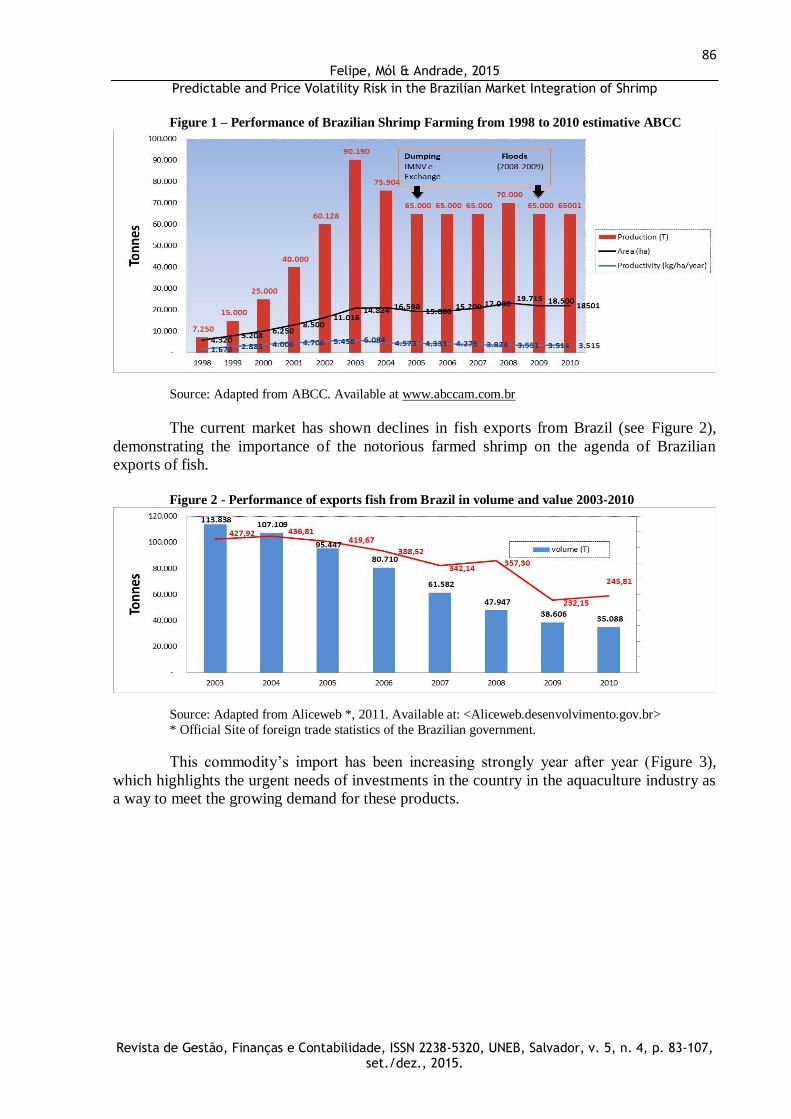
Shrimp farming is taken in this scenario as the main commodity imported into the

Brazilian market. After successive declines in production (2003-2005), the production of

farmed shrimp remained stable from 2005 to 2009 and showed significant increase in 2010,

demonstrating the resilience of the sector, as can be seen in figure (1).




set./dez., 2015.

Figure 1 – Performance of Brazilian Shrimp Farming from 1998 to 2010 estimative ABCC

Source: Adapted from ABCC. Available at www.abccam.com.br

The current market has shown declines in fish exports from Brazil (see Figure 2),

demonstrating the importance of the notorious farmed shrimp on the agenda of Brazilian

exports of fish.

Figure 2 - Performance of exports fish from Brazil in volume and value 2003-2010

Source: Adapted from Aliceweb *, 2011. Available at: <Aliceweb.desenvolvimento.gov.br>

* Official Site of foreign trade statistics of the Brazilian government.

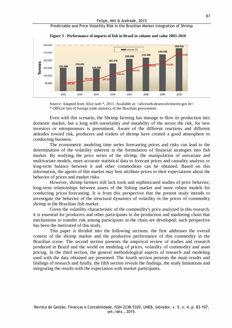
This commodity’s import has been increasing strongly year after year (Figure 3),

which highlights the urgent needs of investments in the country in the aquaculture industry as

a way to meet the growing demand for these products.

http://www.abccam.com.br/




set./dez., 2015.

Figure 3 - Performance of imports of fish in Brazil in volume and value 2003-2010

Source: Adapted from Alice web *, 2011. Available at: <aliceweb.desenvolvimento.gov.br>

* Official Site of foreign trade statistics of the Brazilian government.

Even with this scenario, the Shrimp farming has manage to flow its production into

domestic market, but a long with uncertainty and instability of the sector the risk, for new

investors or entrepreneurs is preeminent. Aware of the different reactions and different

attitudes toward risk, producers and traders of shrimp have created a good atmosphere to

conducting business.

The econometric modeling time series forecasting prices and risks can lead to the

determination of the volatility inherent in the formulation of financial strategies into fish

market. By studying the price series of the shrimp, the manipulation of univariate and

multivariate models, more accurate statistical data to forecast prices and causality analysis or

long-term balance between it and other commodities can be obtained. Based on this

information, the agents of this market may best attribute prices to their expectations about the

behavior of prices and market risks.

However, shrimp farmers still lack tools and sophisticated studies of price behavior,

long-term relationships between assets of the fishing market and more robust models for

conducting prices forecasting. It is from this perspective that the present study intends to

investigate the behavior of the structural dynamics of volatility in the prices of commodity

shrimp in the Brazilian fish market.

Given the volatility characteristic of the commodity's price analyzed in this research,

it is essential for producers and other participants in the production and marketing chain that

mechanisms to transfer risk among participants in the chain are developed; such perspective

has been the motivated of this study.

This paper is divided into the following sections: the first addresses the overall

context of the shrimp market and the productive performance of this commodity in the

Brazilian scene. The second section presents the empirical review of studies and research

produced in Brazil and the world on modeling of prices, volatility of commodity and asset

pricing. In the third section, the general methodological aspects of research and modeling

used with the data obtained are presented. The fourth section presents the main results and

findings of research and finally, the fifth section reveals the findings, the study limitations and

integrating the results with the expectation with market participants.




set./dez., 2015.

2 – EMPIRICAL REVIEW

In literature several studies using time series as methodological tools for forecasting

and price transmission, projected values at risk and identification of long-term relationships

can be found.

Sabes and Alves (2008) investigated the peanut agribusiness by comparing seasonal

patterns of price behavior (1996-2005) and found that seasonal crop and intercrop, influence

the behavior and the dispersion of prices paid to producers in the peanut market. Adami and

Miranda (2011) studied the process of price transmission in the Brazilian rice market and

concluded that the marketing agents from rice production chain may establish marketing

strategies between the two markets (Rio Grande do Sul - RS and Mato Grosso- MT) more

safety when considering that stimulus or discouraging price in RS will affect prices in the MT

market.

Campos et al. (2008) analyzed the causality of cattle prices in different squares in the

Southeast and Midwest regions of Brazil, where they met the result that there is prevalence

between the squares of a dynamic and flexible system for transferring information, and even

that the two regions are not commercially relate to each other, their prices are linked because

both market with a third region.

Campos (2007) gave emphasis to the analysis of the price volatility of agricultural

products in Brazil, and concluded that the cyclical and seasonal fluctuations or the prices of

agricultural products caused as much instability in the producer’s income as in the urban

consumer’s expenses. Furthermore, the author pointed out that the information about volatility

is important for the forecasts of the conditional variance of commodity prices, in an indefinite

horizon. He also stressed that the high risk of price and income associated with the markets

for these products can provide producers and other major economic actors profits in certain

periods, in addition to huge losses and even exit the market in adverse situations.

By using the ARCH approach, Teixeira et al. (2008) investigated the dynamics of the

return volatility on cocoa cattle and coffee commodities. These authors found that the

volatility of the return of cocoa is persistent and indicates that shocks take a long time to

dissipate. Overall, for the three commodities, studied the volatility of returns is persistent and

shocks take a long time to dissipate, and positive and negative shocks have a different impact

on volatility. It was also demonstrated that the estimation results for the conditional mean and

volatility of the returns of coffee, indicate that a shock in the series of returns for various

periods will effect the volatility of these returns.

Concerning volatility, the study of Pereira et al. (2010), aimed at benchmarking the

returns of Brazilian agricultural commodities, where returns of coffee and soya are

characterized by asymmetric responses to the positive and negative shocks, although the

leverage effect has not been identified and VaR measures showed the greatest lost potential to

coffee producers, followed by soya and cattle.

Kreuz and Souza (2006) verified production costs, return expectation and risk of

Garlic agribusiness in southern Brazil. That authors found that in the globalized market

economies there is no way to prevent, without retaliation, imports. Thus, the viability of

Brazilian garlic, mostly from the South, depends on two basic strategies: 1) more research and

development to productivity had increased and 2) choose a product differentiation investing in

purple garlic which is already the Brazilian consumer’s preference.

Moreira et al. (2010) analyzed the agribusiness market’s risk management in the

context of agribusiness cooperatives and through this study has highlighted that the options to

improve the management of market risks (risk-return analysis) and the influence of

agricultural cooperatives in this context, can be made by means of risk-return analysis,

https://www.researchgate.net/publication/273170978_Volatilidade_condicional_dos_retornos_de_commodities_agropecuarias_brasileiras_seguidos_pela_soja_e_pelo_boi_gordo?el=1_x_8&enrichId=rgreq-9b0d370e070052ac786bc71d5f93e96a-XXX&enrichSource=Y292ZXJQYWdlOzI4NjYzNjkwMztBUzozNDIwNjU1OTk3OTUyMDFAMTQ1ODU2NjIwMjQ2Mw==




set./dez., 2015.

performed according to the Markowitz mean variance model. After the application of this

model, an efficiency frontier has been traced which allowed to generate two scenarios of

efficient portfolios (in one of the scenarios was possible greatly decrease the risk associated

with production levels of the portfolio 2006 and in the other, it was possible to increase the

total gross margin for the portfolio maintaining the level of risk practically stable).

On the Shrimp market, the majority of published studies refers only to the qualitative

aspects of production and prices, such as Valenti (2002), Carvalho et al. (2007), Pincinato

(2010) and Ferdouse (2011). On the other hand, the work of Sousa Jr. et al. (2007) and Felipe

et al. (2013) stand out among the works published because they deal with the behavioral

aspects of national and international shrimp prices by univariate and multivariate modeling.

As it was said before, it can be seen that the methodology of time series is

widespread in academia, but its use is restricted only to a few commodities of agribusiness

and agriculture. From the development of this study it is hoped that the information contained

and presented may function as a basis for formation of marketing strategies shrimp in the

Brazilian shrimp market.

Finally, this work was developed with the prospect of adding to the scarce literature

on studies of volatility in the aquaculture sector from a univariate approach applied to the

prices of brazilian medium shrimp. Internationally, there are not many records of work with

the theme and research that this article which is proposing to do. Some studies found

containing fragments of the studies presented here can be seen in Parsons and Colbourne

(2000), Khaemasunun [sd] and Harri, Muhammad and Jones (2010) and Sousa Júnior et al.

(2007).

3 - GENERAL METHODOLOGICAL ASPECTS

This study is presented as an descriptive research of an applied nature with a

quantitative approach through documentary analysis. The price series were extracted from the

database of CEAGESP, (Society of General Warehouses of São Paulo).

The series analyzed represent average prices of shrimp in size between 09G-11g, the

type Litopenaeus Vannamei, as set by the most liquid asset in terms of the marketing of

Brazilian fish. The data correspond to monthly average trading prices quoted by CEAGESP

the timeframe from January 2000 to May 2012. The prices collected represent the Brazilian

market for shrimp. The CEAGESP collects and the price of those prices at national level. To

perform the statistical tests, modeling and forecasting of prices between the price series

shrimp, R (R-Project in version 2.14.2) free software was used.

In this study the methodology ADF (Dickey and Fuller, 1979) and the model of

Enders (2004) for testing and evaluation of the hypothesis of stationarity of the price series

was used.

The univariate model was also applied into the original series of prices of shrimp,

deflated in the series and the series of returns for the purpose of describing the behavior of

prices. SARIMA processes were used in these price series along with procedures for forecasts

𝑦𝑡 12 steps forward and one step ahead of 𝑦𝑡 de horizon 12 Methodology Box-Jenkins (1976),

into the sample with the previous twelve observations.

To prevent unusual phenomena would determine biases in the estimates if they were

not controlled, a study was made of structural break in the period 2010-2012, due to the

strong break in prices in this period. Qualitative variables that could cause biases in the

estimates were modeled by inclusion of seasonal dummies variables.

3.1 Model for price forecasting

https://www.researchgate.net/publication/243644934_Distribution_of_the_Estimators_for_Autoregressive_Time_Series_With_a_Unit_Root?el=1_x_8&enrichId=rgreq-9b0d370e070052ac786bc71d5f93e96a-XXX&enrichSource=Y292ZXJQYWdlOzI4NjYzNjkwMztBUzozNDIwNjU1OTk3OTUyMDFAMTQ1ODU2NjIwMjQ2Mw==




set./dez., 2015.

3.1.1 Seasonal ARIMA or SARIMA

Following the concept proposed by Nelson (1973) and considering that an auto-

regressive stochastic model purely seasonal SAR (P) of order P, one 𝑦𝑡 stationary series is

regressed on its lagged values earlier in multiples of s: 𝑦𝑡 = 𝜙1𝑦𝑡−𝑠 + 𝜙2𝑦𝑡−2𝑠 + ⋯ + 𝜙𝑝𝑦𝑡−𝑃𝑠 + 𝜀𝑡

In turn, the seasonal pattern of pure moving average SMA (Q) of order q can be

represented algebraically by:

𝑦𝑡 = 𝜀𝑡 − 𝜃1𝜀𝑡−𝑠−𝜃2𝜀𝑡−2𝑠− ⋯ − 𝜃𝑄𝜀𝑡−𝑄𝑠

Seasonal combining the auto-regressive moving average terms and has a SARMA (P,

Q), expressed in the form: 𝑦𝑡 = 𝜙1𝑦𝑡−𝑠 + 𝜙2𝑦𝑡−2𝑠 + ⋯ + 𝜙𝑝𝑦𝑡−𝑃𝑠 + 𝜀𝑡 − 𝜃1𝜀𝑡−𝑠−𝜃2𝜀𝑡−2𝑠− ⋯ − 𝜃𝑄𝜀𝑡−𝑄𝑠 (3)

Similarly, as in Examples (models) regular, it can be shown that: 𝛷𝑃(𝐵𝑠) = 1 − 𝜙1𝐵𝑠− 𝜙2𝐵2𝑠− ⋯ − 𝜙𝑃𝐵𝑃𝑠

𝛩𝑃(𝐵𝑠) = 1 − 𝜃1𝐵𝑠− 𝜃2𝐵2𝑠− ⋯ − 𝜃𝑄𝐵𝑄𝑠

For a SAR (P) model, one has: 𝛷𝑃(𝐵𝑠)𝑦𝑡 = 𝜀𝑡

Already for a SMA (Q): 𝑦𝑡 = 𝛩𝑄(𝐵𝑠)𝜀𝑡

and the SARMA model (P, Q): 𝛷𝑃(𝐵𝑠)𝑦𝑡 = 𝛩𝑄(𝐵𝑠)𝜀𝑡

In addition, the auto-regressive and moving average, seasonal models may also be

manipulated to non-stationary series, at the time d-th difference leads to seasonal series

stationarity transformed. This occurring, the model is seasonally integrated order will be

called SARIMA.

The combination product regular seasonal stochastic components model itself is

represented in SARIMA (p, d, q) x (P, D, Q) can be synthesized in the following manner: 𝜙𝑝(𝐵) (1 − 𝐵)d𝛷𝑃(𝐵𝑠)(1 − 𝐵𝑠)D𝑦𝑡 = 𝜃𝑞 (𝐵)𝛩𝑄(𝐵𝑠)𝜀𝑡 (4)

Where it is known that:

𝜙𝑝(𝐵) = the regular operator coefficients of autoregression, whose order is p.

(1 − 𝐵)d = operator ¬D-th regular difference.

𝛷𝑃(𝐵𝑠) = operator coefficients of seasonal autoregression, whose order is P.

(1 − 𝐵𝑠)D operator D = D-th seasonal difference, with periodicity s.

𝜃𝑞 (𝐵) = operator coefficients of the regular moving average of order q.

𝛩𝑄(𝐵𝑠) = operator coefficients of seasonal moving average of order Q.

The process of obtaining the SARIMA model follows the same procedures as the

Box-Jenkins methodology used to meet the non-seasonal ARIMA model. This indicates that

the SARIMA, considering the observance of the behavior of autocorrelation (AFC) and partial

autocorrelation (PACF), however, observed seasonal lags (monthly, weekly, daily serials,

etc.).




set./dez., 2015.

4 - DISCUSSION AND ANALYSIS OF THE RESULTS

4.1 Initial inspections in the price series of the Brazilian medium shrimp

4.1.1 Graphical display of the original price series

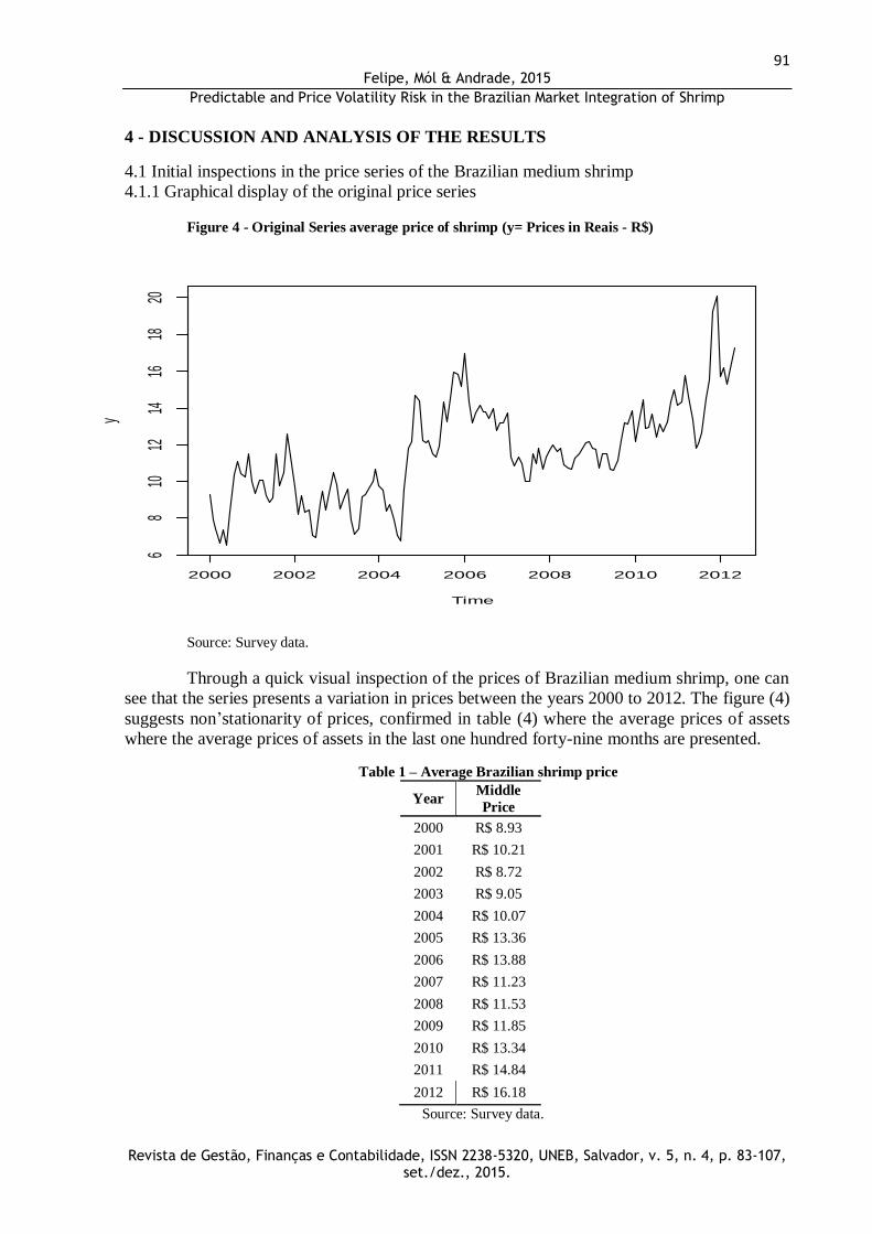
Figure 4 - Original Series average price of shrimp (y= Prices in Reais - R$)

Source: Survey data.

Through a quick visual inspection of the prices of Brazilian medium shrimp, one can

see that the series presents a variation in prices between the years 2000 to 2012. The figure (4)

suggests non’stationarity of prices, confirmed in table (4) where the average prices of assets

where the average prices of assets in the last one hundred forty-nine months are presented.

Table 1 – Average Brazilian shrimp price

Year Middle

Price

2000 R$ 8.93

2001 R$ 10.21

2002 R$ 8.72

2003 R$ 9.05

2004 R$ 10.07

2005 R$ 13.36

2006 R$ 13.88

2007 R$ 11.23

2008 R$ 11.53

2009 R$ 11.85

2010 R$ 13.34

2011 R$ 14.84

2012 R$ 16.18


Time

y

2000 2002 2004 2006 2008 2010 2012

68

1012

1416

1820




set./dez., 2015.

The great variability in prices over the years was caused among other factors, by the

american antidumping measure, where production went from 76,000 tons to 65,000 in 2005

(see figure 1), which resulted in a loss of productivity that was 6,084 (kg / ha / year) in 2004

to 3,515 (kg / ha / year) in 2010 (see figure 1), the decline in exports both in volume and in

value (decline since 2003 - see figure 2) and the growth of imports both in volume and in

value (increase since 2006 - see figure 3), which do generate foreign currency and devaluation

of the brazilian currency in international trade in commodities.

Based on information from the figure (4) and table (1), traders and investors can have

some clarification about the variation in the price of shrimp. Where the higher valuation of the

asset was given only in 2012 when the average price was R$ 16.18 and the reflection of the

American added measure with the flooding in yields (due to the heavy rain) was the

devaluation of the average price of shrimp which was R$ 13.36 and R $ 11.85 went to in

2009.

All this means that voluptuous investments in commodity shrimp did not bring

significant earnings on invested capital at that time (2005-2009). The recovery in average

prices is only noticeable from 2010 onwards.

Continuing with the initial inspection and a detailed statistical description of the

general aspects of the series, the price decomposition was performed under the temporal order

in an additive graph as we can see in figure (5).

4.1.2 Additive decomposition of shrimp prices in temporal series

Figure 5 - additive decomposition of shrimp prices in temporal series





set./dez., 2015.

The graph of additive decomposition allows a better insight into the initial price

dynamics. Price variability is shown in the first quadrant of the figure (5). In the second

quadrant, it shows the estimated trend of the series of prices which presents an increasing

behavior. In the third quarter of the same graph, estimated effects of seasonality in prices can

be viewed. It’s worth noting that the evidence of nonstationarity was confirmed by ADF test

and can be seen in the figure below.

Table 2 – Augmented Dickey-Fuller Test

Augmented Dickey-Fuller Test

Dickey-Fuller = -3.4324

p-value = 0.05187

____________________________________________________

*Alternative hypothesis: stationary


The last quadrant shows a perspective view on the random term of the series of

prices, which in turn, shows a great variability, but a reasonably stable balance (indication of

stationarity). For a more rigorous inspection, a test on the first difference of the price series

was performed (see figure 6).

4.1.3 Graphical Inspection of the first difference of the shrimp prices series (dy)

Figure 6 - First-difference of the Shrimp prices series





set./dez., 2015.

The first difference of the original price series appears to be stationary, which will be

checked with other inspections and formal statistical tests before making inferences about

behavior and temporal dynamics of the price series.

As follows autocorrelation functions (ACF) and partial autocorrelation (PACF) were

examined, which can be seen in figure (7) and (8). The behavior of these functions indicates

the models to be used, as well as assists in the use of unit root tests to confirm the stationarity.

4.1.4 Autocorrelation Function - ACF -for the lagged shrimp price series (dy)

Figure 7 - ACF correlogram for the lagged shrimp prices series (dy)


The ACF function is the graph of autocorrelation against the lag. In different series

(dy) one realizes that the problem of autocorrelation data was well resolved when it was

originally making a difference in the number of shrimp prices and information correlated over

time are minimized.

When one takes a difference and the ACF decays exponentially fast, reaching almost

zero in the first lags, it is the sign that we can work with a simple model AR (1) .For the price

series under study, the AR model (1) is a good candidate to be chosen for modeling and

forecasting prices, but this is still not enough to choose it, because the effects of seasonality

were not resolved, as it was appointed by the initial inspection in (5) and the models this

modeling are sought are those that produce waste in the form of white noise.

Next, a graphical inspection will be done on the partial autocorrelation function for

the number of shrimp prices with a lag, once we saw earlier, that with a difference, it may

reach the stationary lagged series (see figura 8).




set./dez., 2015.

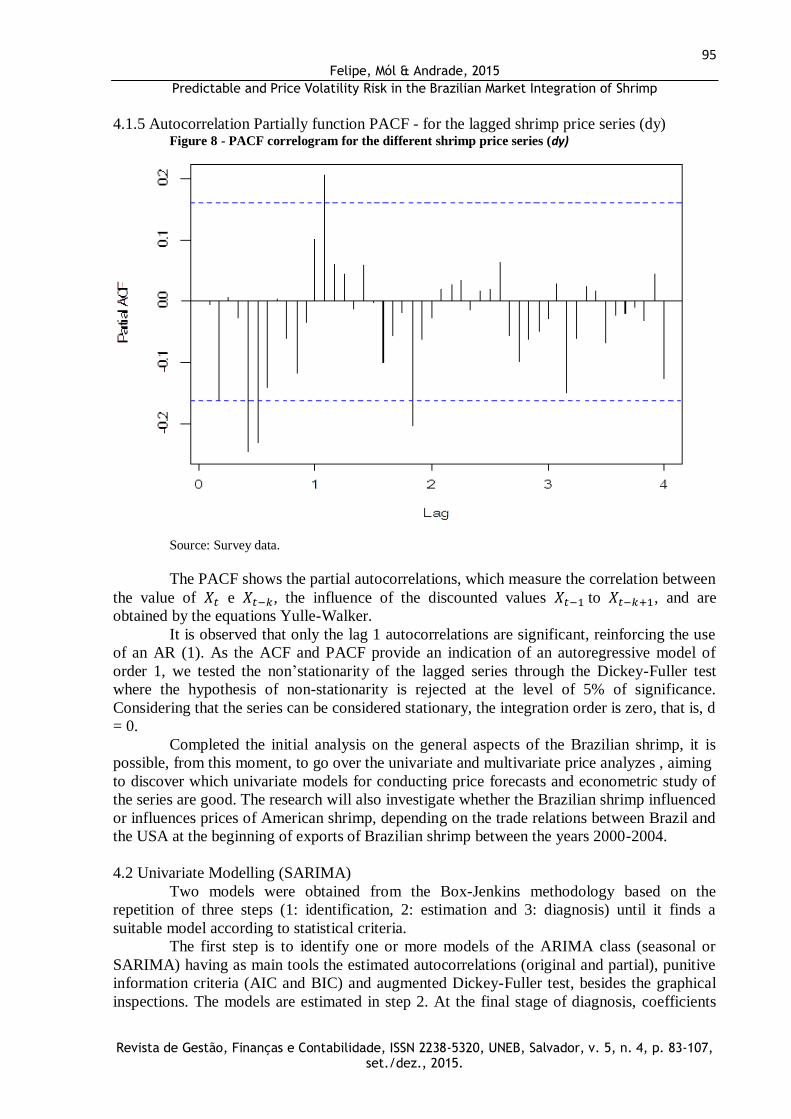
4.1.5 Autocorrelation Partially function PACF - for the lagged shrimp price series (dy)

Figure 8 - PACF correlogram for the different shrimp price series (dy)


The PACF shows the partial autocorrelations, which measure the correlation between

the value of 𝑋𝑡 e 𝑋𝑡−𝑘, the influence of the discounted values 𝑋𝑡−1 to 𝑋𝑡−𝑘+1, and are

obtained by the equations Yulle-Walker.

It is observed that only the lag 1 autocorrelations are significant, reinforcing the use

of an AR (1). As the ACF and PACF provide an indication of an autoregressive model of

order 1, we tested the non’stationarity of the lagged series through the Dickey-Fuller test

where the hypothesis of non-stationarity is rejected at the level of 5% of significance.

Considering that the series can be considered stationary, the integration order is zero, that is, d

= 0.

Completed the initial analysis on the general aspects of the Brazilian shrimp, it is

possible, from this moment, to go over the univariate and multivariate price analyzes , aiming

to discover which univariate models for conducting price forecasts and econometric study of

the series are good. The research will also investigate whether the Brazilian shrimp influenced

or influences prices of American shrimp, depending on the trade relations between Brazil and

the USA at the beginning of exports of Brazilian shrimp between the years 2000-2004.

4.2 Univariate Modelling (SARIMA)

Two models were obtained from the Box-Jenkins methodology based on the

repetition of three steps (1: identification, 2: estimation and 3: diagnosis) until it finds a

suitable model according to statistical criteria.

The first step is to identify one or more models of the ARIMA class (seasonal or

SARIMA) having as main tools the estimated autocorrelations (original and partial), punitive

information criteria (AIC and BIC) and augmented Dickey-Fuller test, besides the graphical

inspections. The models are estimated in step 2. At the final stage of diagnosis, coefficients




set./dez., 2015.

and their standard errors are valued, where the main statistical characteristics of the waste in

each model should appear as white noise.

At diagnosis, similar tools to the first stage were used, but applying the waste instead

of the original series: estimated autocorrelations (original and partial), the Box-Ljung test and

graphical inspection. In this second step, the previously selected models are changed or

dropped or added to new models and the process can be repeated two or three times until you

have a small number of suitable models. In case of more than one final model, forecasts can

be used for possible tiebreaker.

a) Modeling with the original series (w and y)

The model resulting from the analysis described in the introduction based on the

number of 𝑦𝑡 prices was a SARIMA (13,1,0)(1,0,0)12, specifically:

(1 + 0,17𝐵2 + 0,25𝐵5 − 0,23𝐵13)(1 − 0,22𝐵12)∆𝑦𝑡 = 𝜀𝑡 (1)

Table 2 – Model results of the Sarima (13,1,0)(1,0,0)12

Coefficients: ar1 ar2 ar3 ar4 ar5 ar6 ar7

0 -0,1703 0 0 -0,2547 0 0

S.E: 0 0,0155 0 0 0,0165 0 0

ar8 ar9 ar10 ar11 ar12 ar13 sar1

0 0 0 0 0 0,2304 0,2171

S.E: 0 0 0 0 0 0,0172 0,0222

1,092

AIC: 444,73


Thus, the stationarity of the original price series was obtained after a simple

difference and the model produces waste in the form of white noise with an estimated

variance of 1.1. All estimated coefficients of the model have p-value less than 1%. The waste

of the models showed a strong adherence to the normal distribution (quantile viewing and

usual normality tests) and no additives or innovation outliers were detected.

It was also observed that a second model SARIMA, this time with a seasonal

difference, showed similar results, but lower in terms of predictions. On the other hand,

regarding to the deflated series, the opposite happened, in other words, the SARIMA model

with seasonal difference was higher (see next section).

Figure 9: Forecast 𝒀𝒕 12 steps ahead. The dashed line represents the point forecast and the dotted lines

represent the limits of the forecast range of 95%. rEMQP 2.6 and MAPE of 13.2%


Time

w

2010.0 2010.5 2011.0 2011.5 2012.0

1012

1416

18




set./dez., 2015.

Shortly thereafter, the forecast of the series into two scenarios (forecast yt 12 steps

forward and one step ahead prediction of yt de horizon 12), where in both cases, we used the

model described above and forecasts were made based on it of the previous twelve

observations (within the sample).

The first procedure (figure 9) is more robust and provides forecasts for one year

ahead, i.e., twelve steps in relation to the last observation. Through a quick visual inspection,

it is observed that the predictions show strong deviations from what happens in reality. The

mean absolute percentage error (MAPE), which represents the absolute difference between

the predicted and actual values, was 13.2%, which indicates a high degree of forecast error.

Besides MAPE presented in high value, the first procedure also showed a mean squared error

(rEMQP) 2.6. It is worth noting that it is an unusual and difficult period to predict for the

observations 2012: 11 and 2012: 12, due to the present a strong structural break in the

behavior of prices.

In the second procedure (figure 10), predictions were made by the method step by

step, where each prediction is made in isolation, just considering the previous prediction, thus

the ASM showed a value of 2.8%, which according to Heizer and Render (2004), indicates an

acceptable value for prediction errors as well as an average squared error (rEMQP) of 0.6 and

a better quality of prediction regarding the procedure (1).

Figure 10 - Forecast one step ahead of 𝐲𝐭 de horizon 12. The dashed line represents the point

forecast and the dotted lines represent the limits of the forecast range of 95%. rEMQP 0.6 to

2.8% MAPE


b) Modeling with deflated series (w and y)

For deflating of the original shrimp price series, we used the IGP-DI based in 2011:

12 (figure 11). The SARIMA (1,1,0) (1,1,0) model produced errors similar to white noise (see

table 2), (1 + 0,19𝐵)(1 + 0,54𝐵12)∆∆12𝑦𝑡 = 𝜀𝑡 (2)

resulting in waste with estimated variance of 3.2. The autoregressive coefficient is significant

at the 5% level and the seasonal autoregressive coefficient is significant at the 1% level.

Time

y

2010.0 2010.5 2011.0 2011.5 2012.0

1015

20




set./dez., 2015.

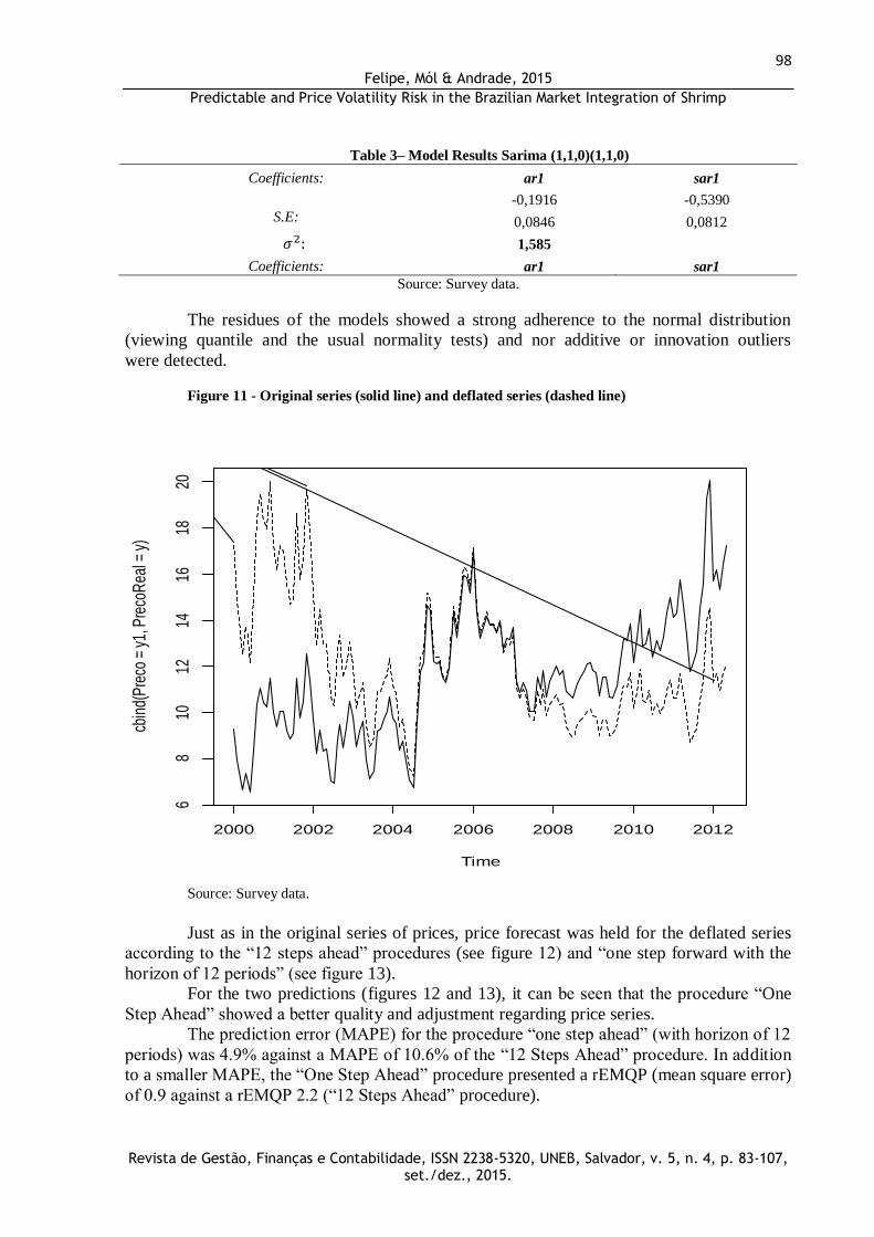
Table 3– Model Results Sarima (1,1,0)(1,1,0)

Coefficients: ar1 sar1

-0,1916 -0,5390

S.E: 0,0846 0,0812

1,585

Coefficients: ar1 sar1


The residues of the models showed a strong adherence to the normal distribution

(viewing quantile and the usual normality tests) and nor additive or innovation outliers

were detected.

Figure 11 - Original series (solid line) and deflated series (dashed line)


Just as in the original series of prices, price forecast was held for the deflated series

according to the “12 steps ahead” procedures (see figure 12) and “one step forward with the

horizon of 12 periods” (see figure 13).

For the two predictions (figures 12 and 13), it can be seen that the procedure “One

Step Ahead” showed a better quality and adjustment regarding price series.

The prediction error (MAPE) for the procedure “one step ahead” (with horizon of 12

periods) was 4.9% against a MAPE of 10.6% of the “12 Steps Ahead” procedure. In addition

to a smaller MAPE, the “One Step Ahead” procedure presented a rEMQP (mean square error)

of 0.9 against a rEMQP 2.2 (“12 Steps Ahead” procedure).

Time

cbin

d(P

reco

= y

1, P

reco

Rea

l = y

)

2000 2002 2004 2006 2008 2010 2012

68

1012

1416

1820

𝜎2:




set./dez., 2015.

Figure 12 - Forecast of 12 steps ahead 𝒚𝒕. Dashed line represents the forecast point and the

traced lines represent the limits of the 95% prediction interval. rEMQP 2.2 and MAPE 10.6%


Figure 13 – “One Step Ahead” forecast horizon 𝒚𝒕 12. The dashed line represents the forecast

point and the traced lines represent the limits of the 95% prediction interval. rEMQP 0.9 to

4.9% MAPE


c) Modeling with seasonal exponential smoothing

For the original series the Holt-Winters model made the following estimates for the

level parameters, trend and seasonality respectively: α = 0.58, β = 0 and γ = 0.49. As for the

deflated series a greater weight to reduction in component and seasonal effect level was

obtained: α = 0.42, β = γ = 0.01 and 0.70.

This higher value of γ confirms the need to use a seasonal difference when working

with the deflated series (see models (1) and (2)). The horizon forecasts 12, both a year ahead

as well as a month (step) forward, are inferior to those obtained by SARIMA models (1) and

(2).

Time

w

2010.0 2010.5 2011.0 2011.5 2012.0

510

1520

Time

y

2010.0 2010.5 2011.0 2011.5 2012.0

1015

20




set./dez., 2015.

d) Modeling with the number of returns (percentage change in prices - r)

One of the approaches to the study of asset prices is the continuous modeling of

returns, where:

𝑟𝑡 = 𝐿𝑛𝑃𝑡

𝐿𝑛𝑃𝑡−1 , illustrated in figure (14).

The resulting model of Box-Jenkins methodology (1976) used in previous sections

was a SARIMA (6,0,0) (1,0,0): (1 + 0,27𝐵5 + 0,22𝐵6)(1 − 0,22𝐵12)𝑧𝑡 = 𝜀𝑡 (3)

Table 4– Results models Sarima (6,0,0)(1,0,0)

Coefficients: ar1 ar2 ar3 ar4 ar5 ar6 sar1 intercept

0 0 0 0 -0,2605 -0,2192 0,2166 -0,1068

S.E: 0 0 0 0 0,0801 0,0863 0,0934 0,6353

81,72

AIC: 1083,09


As in (1), a half cycle seasonal effect in addition to seasonal effects and effects of

magnitudes comparable to (1) was observed. The exception would be the lag effect 2 that here

was not significant whereas in (1) a 𝜑2 = -0.17 was obtained. However, this estimate had

borderline significance (p-value less than 5%).

For comparison, if it included the autoregressive term of order 2 in (3) we would

obtain an estimate of -0.13 with p-value between 5% and 10%.The residues of the models

showed a strong adherence to the normal distribution (viewing quantile and the usual

normality tests) and nor additive or innovation outliers were detected

Figure 14 – Returns


𝜎2:




set./dez., 2015.

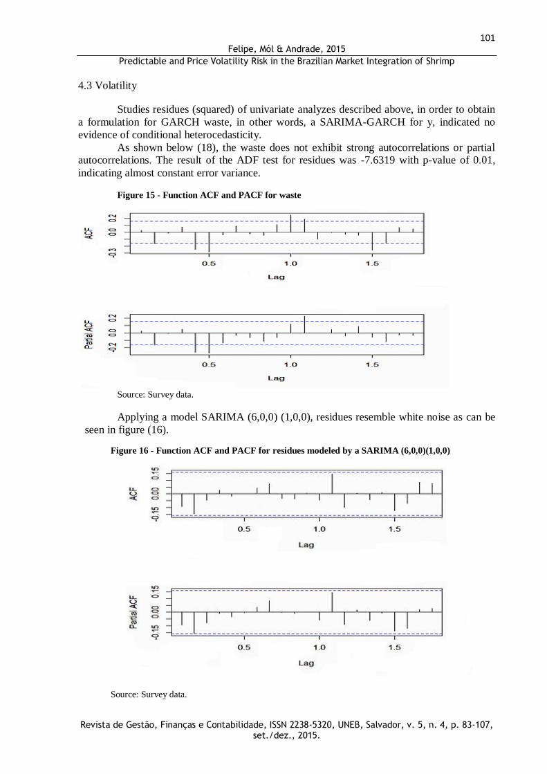
4.3 Volatility

Studies residues (squared) of univariate analyzes described above, in order to obtain

a formulation for GARCH waste, in other words, a SARIMA-GARCH for y, indicated no

evidence of conditional heterocedasticity.

As shown below (18), the waste does not exhibit strong autocorrelations or partial

autocorrelations. The result of the ADF test for residues was -7.6319 with p-value of 0.01,

indicating almost constant error variance.

Figure 15 - Function ACF and PACF for waste


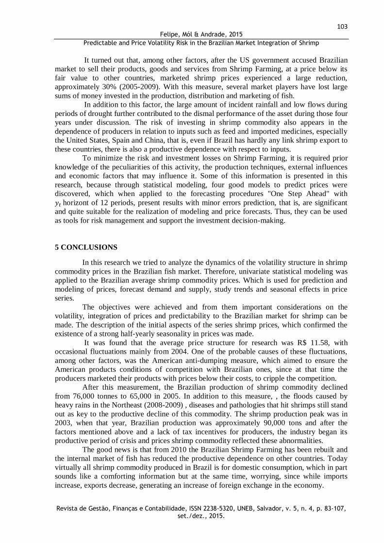
Applying a model SARIMA (6,0,0) (1,0,0), residues resemble white noise as can be

seen in figure (16).

Figure 16 - Function ACF and PACF for residues modeled by a SARIMA (6,0,0)(1,0,0)





set./dez., 2015.

Finally, through the figures (17 and 18), the reason of not using the GARCH model

for unconditional mean and volatility of waste can be confirmed, because the SARIMA

process (6,0,0) (1,0,0) had shaped waste and expectations of large dispersion around the mean

were not confirmed, however, little scatter was found.

Figure 17 - Behaviour of the residue


Figure 18 - residues Distribution


4.4 Integration of search results with the expectations of marketing agents

Through the results presented by this research, the marketing agents of shrimp

commodity can view statistical aspects for more efficient investment management from the

perspective of risk.




set./dez., 2015.

It turned out that, among other factors, after the US government accused Brazilian

market to sell their products, goods and services from Shrimp Farming, at a price below its

fair value to other countries, marketed shrimp prices experienced a large reduction,

approximately 30% (2005-2009). With this measure, several market players have lost large

sums of money invested in the production, distribution and marketing of fish.

In addition to this factor, the large amount of incident rainfall and low flows during

periods of drought further contributed to the dismal performance of the asset during those four

years under discussion. The risk of investing in shrimp commodity also appears in the

dependence of producers in relation to inputs such as feed and imported medicines, especially

the United States, Spain and China, that is, even if Brazil has hardly any link shrimp export to

these countries, there is also a productive dependence with respect to inputs.

To minimize the risk and investment losses on Shrimp Farming, it is required prior

knowledge of the peculiarities of this activity, the production techniques, external influences

and economic factors that may influence it. Some of this information is presented in this

research, because through statistical modeling, four good models to predict prices were

discovered, which when applied to the forecasting procedures "One Step Ahead" with

𝑦𝑡 horizont of 12 periods, present results with minor errors prediction, that is, are significant

and quite suitable for the realization of modeling and price forecasts. Thus, they can be used

as tools for risk management and support the investment decision-making.

5 CONCLUSIONS

In this research we tried to analyze the dynamics of the volatility structure in shrimp

commodity prices in the Brazilian fish market. Therefore, univariate statistical modeling was

applied to the Brazilian average shrimp commodity prices. Which is used for prediction and

modeling of prices, forecast demand and supply, study trends and seasonal effects in price

series.

The objectives were achieved and from them important considerations on the

volatility, integration of prices and predictability to the Brazilian market for shrimp can be

made. The description of the initial aspects of the series shrimp prices, which confirmed the

existence of a strong half-yearly seasonality in prices was made.

It was found that the average price structure for research was R$ 11.58, with

occasional fluctuations mainly from 2004. One of the probable causes of these fluctuations,

among other factors, was the American anti-dumping measure, which aimed to ensure the

American products conditions of competition with Brazilian ones, since at that time the

producers marketed their products with prices below their costs, to cripple the competition.

After this measurement, the Brazilian production of shrimp commodity declined

from 76,000 tonnes to 65,000 in 2005. In addition to this measure, , the floods caused by

heavy rains in the Northeast (2008-2009) , diseases and pathologies that hit shrimps still stand

out as key to the productive decline of this commodity. The shrimp production peak was in

2003, when that year, Brazilian production was approximately 90,000 tons and after the

factors mentioned above and a lack of tax incentives for producers, the industry began its

productive period of crisis and prices shrimp commodity reflected these abnormalities.

The good news is that from 2010 the Brazilian Shrimp Farming has been rebuilt and

the internal market of fish has reduced the productive dependence on other countries. Today

virtually all shrimp commodity produced in Brazil is for domestic consumption, which in part

sounds like a comforting information but at the same time, worrying, since while imports

increase, exports decrease, generating an increase of foreign exchange in the economy.




set./dez., 2015.

Still on the behavior of prices, the original price series presented stationarity,

resolved when it made a difference in the series. The functions of autocorrelation and partial

autocorrelation confirmed that with a difference stationarity could be well solved, but the

series still indicated a strong seasonality. Therefore, more rigorous processes were used for

statistical modeling of prices. We selected four models for the achievement of price

forecasting and description of active behavior. The model chosen for the number of shrimp

original price was the SARIMA process (13,1,0)(1,0,0)12, residues of which presented

themselves as white noise. For the series of deflated prices, the SARIMA process

(1,1,0)(1,1,0), was chosen, depending on its significance and its adjustment to the

achievement of price forecasts.

Another good model to model the shrimp price series was the seasonal exponential

smoothing Holt-Winters method (HW) as its coefficients explained approximately 60% of the

level and 80% of the seasonality of the original series and deflated series.

The last selected model was the percentage change in prices (or returns), the

SARIMA process (6,0,0) (1,0,0), as well as those mentioned above, produced residues as

white noise and introduced itself as a good predictor of a modeling point of view of price.

Given the several models tested, these four models mentioned above showed good

statistical significance and low errors standards, showing good candidates for the realization

of price forecasts. The methodology "One Step Ahead" with 12 periods horizon 𝑦𝑡, presented

as the most statistically robust among other tested, because it indicated lower forecast errors

compared the original price series.

The contribution of this research lies in the application of sophisticated techniques

of time series analysis combined with investment risk management in commodities. Through

statistical modeling, it was possible to understand the behavior of the relevant facts and

aspects of price and seasonal effects that affect the earnings of market players in the industry

of shrimp farming.

Finally, bearing the information gathered in this work, with the implementation of

the methods and statistical techniques discussed here, it is expected that producers and shrimp

traders can have more strategic devices to achieve higher returns for their investments in the

fish market and as result, this market continue fostering the economy, generating jobs and

income in the northeastern regions of Brazil.

REFERENCES

ABCC - ASSOCIAÇÃO BRASILEIRA DE CRIADORES DE CAMARÃO. Estatística do

setor pesqueiro. Available in: <http://www.abccam.com.br.>. Acess: 20 fev. 2012.

ADAMI, A. C. de O.; MIRANDA, S. H. G. de. Transmissão de Preços e Cointegração no

Mercado Brasileiro de Arroz. RESR, São Paulo. v. 49, n.1, p. 55-80, 2011.

ALICEWEB. Estatísticas do comércio. Available in: <

http://www.desenvolvimento.gov.br/sitio/interna/interna.php?area=5&menu=608&refr=608.>

. Acess: 29 fev. 2014.

ASSOCIAÇÃO BRASILEIRA DE CRIADORES DE CAMARÃO. O Agronegócio do

camarão marinho cultivado. Recife: ABCC, jul., p.3, 2002.

http://www.abccam.com.br/




set./dez., 2015.

BOX, G.E.P.; JENKINS, G.M.; REINSEL, G.C. Time series analysis: forecasting and

control. 3th ed. San Francisco: Holden-Day, 1976.

CAMPOS, K. C. C. Análise da volatilidade de preços de produtos agropecuários no

Brasil. 2007. Available in:< www.sober.org.br/palestra/6/486.pdf>. Acess: 02 jan. 2014.

CAMPOS, S. K.; SILVA, A. F.; COSTA, J.S.; ZILLI, J.B. Análise da cointegração e

causalidade dos preços de boi gordo em diferentes praças nas regiões sudeste e centro-

oeste do Brasil. Available in: <ftp://ftp.sp.gov.br/ftpiea/publicar/REA2-1208a7.pdf>

Acess: 23 jun. 2014. Publication date: jul/dez. 2008.

CARVALHO, R.A.P.L.F. de. RUIVO, U.E.; ROCHA, I. de P. R. Mercado interno: situação e

oportunidades para o camarão brasileiro. Panorama da Aquicultura, jun., 2007.

DICKEY, D.A.; FULLER W.A. Distribution of the Estimators for Autoregressive Time

Series with a Unit Root. Journal of the American Statistical Association, v.74, p 427–431,

1979

ENDERS, Walter. Applied Econometric Time Series. 2nd ed. USA: John Willey & Sons,

2004.

FELIPE, I.J. dos S.; MÓL, A. L.R; ALMEIDA, V. de S. Evidências na projeção de Value-at-

Risk em preços de camarão no Brasil via modelagem ARIMA com erros GARCH. Custos e

@gronegócio online. v. 9, 3nd, 2013.

FERDOUSE, F. Tendências da demanda asiática por produtos da aquicultura. Available

in:<http://dc415.4shared.com/doc/oRXADe18/preview.html>. Acess: 28 jun. 2014. .

Publication date: jul/dez. 2009.

FULLER, W.A. Introduction to statistical time series. New York: John Wiley & Sons,

1976.

HARRI, A.; MUHAMMAD, A.; JONES, K. Market Integration for Shrimp and the Effect

of Catastrophic Events. Available in:

<http://ageconsearch.umn.edu/bitstream/61585/2/AAEA%202010%20Shrimp.pdf>. Acess:

02 jun. 2014. Publication date: jul 2010.

HEIZER, J.; RENDER, B. Operations management. 7ª ed. Upper Saddle River, NJ: Pearson

Education, 2004.

KHAEMASUNUN, P. Forecasting Thai Gold Prices. Available in: <

http://www.wbiconpro.com/3-Pravit-.pdf>. Acess: 02 jun. 2014.

KREUZ, C. L.; SOUZA, A. Custos de Produção, Expectativas de Retorno e de Risco do

Agronegócio do Alho no Sul do Brasil. Available

in:<http://www.unisinos.br/abcustos/_pdf/ABC_KreuzSouza.pdf>. Acess: 25 jun. 2014. .

Publication date: set/dez 2006.

http://dc415.4shared.com/doc/oRXADe18/preview.html

http://ageconsearch.umn.edu/bitstream/61585/2/AAEA%202010%20Shrimp.pdf

http://www.wbiconpro.com/3-Pravit-.pdf

http://www.unisinos.br/abcustos/_pdf/ABC_KreuzSouza.pdf

https://www.researchgate.net/publication/269504318_Time_Series_Analysis_Forecasting_and_Control?el=1_x_8&enrichId=rgreq-9b0d370e070052ac786bc71d5f93e96a-XXX&enrichSource=Y292ZXJQYWdlOzI4NjYzNjkwMztBUzozNDIwNjU1OTk3OTUyMDFAMTQ1ODU2NjIwMjQ2Mw==

https://www.researchgate.net/publication/269504318_Time_Series_Analysis_Forecasting_and_Control?el=1_x_8&enrichId=rgreq-9b0d370e070052ac786bc71d5f93e96a-XXX&enrichSource=Y292ZXJQYWdlOzI4NjYzNjkwMztBUzozNDIwNjU1OTk3OTUyMDFAMTQ1ODU2NjIwMjQ2Mw==




https://www.researchgate.net/publication/254384009_Market_Integration_for_Shrimp_and_the_Effect_of_Catastrophic_Events?el=1_x_8&enrichId=rgreq-9b0d370e070052ac786bc71d5f93e96a-XXX&enrichSource=Y292ZXJQYWdlOzI4NjYzNjkwMztBUzozNDIwNjU1OTk3OTUyMDFAMTQ1ODU2NjIwMjQ2Mw==









https://www.researchgate.net/publication/239418534_Applied_Econometric_Time_Series_2?el=1_x_8&enrichId=rgreq-9b0d370e070052ac786bc71d5f93e96a-XXX&enrichSource=Y292ZXJQYWdlOzI4NjYzNjkwMztBUzozNDIwNjU1OTk3OTUyMDFAMTQ1ODU2NjIwMjQ2Mw==

https://www.researchgate.net/publication/239418534_Applied_Econometric_Time_Series_2?el=1_x_8&enrichId=rgreq-9b0d370e070052ac786bc71d5f93e96a-XXX&enrichSource=Y292ZXJQYWdlOzI4NjYzNjkwMztBUzozNDIwNjU1OTk3OTUyMDFAMTQ1ODU2NjIwMjQ2Mw==




set./dez., 2015.

MDIC. Ministério do desenvolvimento, Indústria e Comércio Exterior. Available in:<

http:// www.mdic.gov.br/arquivos/dwnl_1329393797.doc>. Acess: 12 abr. 2014.

MOREIRA, V.R.; PROTIL, R.M.; DA SILVA, C.L. Gestão dos riscos de mercado do

agronegócio no contexto das cooperativas agroindustriais. Available in:<

http://www.sober.org.br/palestra/15/919.pdf>. Acess: 25 jun. 2014. Publication date: jun

2010.

NELSON, C. R. Applied time series analysis for managerial forecasting. San Francisco:

Holden-Day, 1973.

NMFS-NOAA. Office of Science & Technology. Available in:<

http://www.st.nmfs.noaa.gov/st1/trade/cumulative_data/TradeDataProduct.html>. Acess: 12

jun. 2014.

PARSONS, D.G.; COLBOURNE, E.B. Forecasting Fishery Perfomance for Northern

Shrimp (Pandalus borealis) on the Labrador Shelf. Disponível

em<http://journal.nafo.int/J27/Parsons.pdf>. Acess: 02 jun. 2014. Publication date: 2000.

PINCINATO, R.B. M. Análise ecológica e econômica da pesca marinha por meio de

indicadores multiespecíficos. Available in:<

http://www.bv.fapesp.br/pt/bolsas/107777/analise-ecologica-economica-pesca-marinha/>.

Acess: 22 jun. 2014. Publication date: 2010.

PEREIRA, V. da F.; LIMA, J. E. de. BRAGA, M. J.; MENDONÇA, T. G. de. Volatilidade

condicional dos retornos de commodities agropecuárias brasileiras. Revista de Economia, v.

36, n. 3, p. 73-94, 2010.

PIMENTEL, E. A.; ALMEIDA, L.; SABBADINI, R. Comportamento recente das

exportações agrícolas no Brasil: uma análise espacial no âmbito dos estados. In: Congresso

brasileiro de economia e sociologia rural, 42, Cuiabá, 2004.

SABES, J. J. S.; ALVES, A.F. O agronegócio do amendoim: estudo e comparação dos

padrões sazonais de comportamento dos preços no período de janeiro de 1996 a

dezembro de 2005. Available in: <http://www.sober.org.br/palestra/9/533.pdf.> Acess: 03

jun. 2014. Publication date: jul. 2008.

SOUSA JÚNIOR, J. P.; TEIXEIRA, K. H.; LIMA, R. C. Camarão brasileiro: uma análise

comportamental dos preços nacional e internacional. Revista de Política Agrícola, v. 3, p.

66-75, 2007.

TEIXEIRA, G. S.; MAIA, S. F.; FIGUEIREDO, N. M.; PEREIRA, E.S.; ALMEIDA PINTO,

P. A. L. de. Dinâmica da Volatilidade do Retorno das Principais Commodities

Brasileiras: uma abordagem dos modelos ARCH. Disponível em:<

http://ageconsearch.umn.edu/bitstream/109785/2/544.pdf>. Acesso em: 23 jun. 2014.

Publication date: jul. 2008.

http://www.sober.org.br/palestra/15/919.pdf

http://www.st.nmfs.noaa.gov/st1/trade/cumulative_data/TradeDataProduct.html

http://journal.nafo.int/J27/Parsons.pdf

http://www.bv.fapesp.br/pt/bolsas/107777/analise-ecologica-economica-pesca-marinha/

http://www.sober.org.br/palestra/9/533.pdf







set./dez., 2015.

VALENTI, W. C. 2002. Criação de camarões de água doce. In: Congresso de Zootecnia,

12º, Vila Real, Portugal, 2002, Vila Real: Associação Portuguesa dos Engenheiros

Zootécnicos. Anais... p. 229-237.

Date post:	19-Sep-2018
Category:	Documents
Upload:	phamthien
View:	219 times
Download:	0 times

Predictable and price volatility risk in the brazilian ... · Predictable and price volatility risk...

Documents