Predicting 100-year peakflows for small forested

tributaries of the Skagit and Samish Rivers

May 7, 2001

Curt Veldhuisen – Hydrologist Richard Haight – Forester

Skagit System Cooperative 25944 Community Plaza Way Sedro Woolley, WA 98284

(360) 856-5501

I. Introduction I a. Peakflows and Project Design Despite their infrequent occurrence, major peakflows (>25-year recurrence, or annual probability <4%) play a major role in damaging road crossings and other stream-associated structures (Furniss et al. 1998), often resulting in both serious economic costs and significant aquatic habitat impacts (Hayman et al. 1991). An easily applied method for estimating streamflow rates during high-magnitude events can be valuable for a variety of design applications, including road crossing structures and habitat enhancement projects. Though various peakflow magnitudes (e.g. 2-year, 10-year, or 100-year) are relevant to different projects, the 100-year magnitude often represents the upper design standard for hydraulic capacity, and has recently been adopted as the regulatory design standard for forest road crossings (previously 50-year), as well. Realistic peakflow estimates for small watersheds (basin area <10 mi2) are particularly useful, since small streams constitute the largest number of road crossings across the landscape, and thus the largest number of potential failure sites. I b. Peakflow Prediction Methods Peakflow response varies considerably between small watersheds and it is generally recognized that such differences reflect the influence of various watershed conditions including soils, vegetation and land use in addition to precipitation inputs (Dunne and Leopold 1978). However, because the level of effort required to account for all such basin attributes in peakflow estimation is prohibitive for most basins, regional empirical regression equations are commonly used for ungaged streams. Such prediction equations are developed from historic peakflow data collected at comparable gaged basins, and generate peakflow estimates on the basis of one or two key basin attributes, typically basin area and annual precipitation. Because only two basin attributes are accounted for directly, the accuracy of the peakflow estimates depends to a large extent on the similarity of the ungaged stream being analyzed to the pool of gaged streams that was used to develop the regression equation. I c. Project Objective The objective of this analysis is to identify a simple and relatively accurate method for estimating the 100-year peakflow for small, forested tributaries to the Skagit and Samish Rivers (Water Resources Inventory Areas #3 & 4), the watersheds of interest to the Skagit System Cooperative (S.S.C.). The primary application of this method is for the design of forest road crossings. The accuracy of peakflow estimates is especially important for very small watersheds (basin area <1.0 mi2 or 640 acres), since these stream crossings typically utilize culverts, which are amenable to simple hydraulic design. In contrast, road crossings of larger streams normally utilize bridges that provide such abundant channel clearance that capacity analysis is unnecessary. II. Approach and Analysis This analysis consisted of five steps, each documented further in the remainder of this report:

a. Identify small gaged forested tributaries to the Skagit and Samish Rivers with sufficient period of record (> 10 years) to estimate 100-year peakflows.

b. Identify existing peakflow prediction methods applicable to the study area. c. Develop a new prediction method using local gaging data identified in step ‘a’ above. d. Evaluate the accuracy of existing and new methods by comparison of estimates to gage-based

peakflows and select the best predictive method. e. Provide guidance for application of the recommended method.

Peakflows for small Skagit tributaries 1 Final Report – May 7, 2001

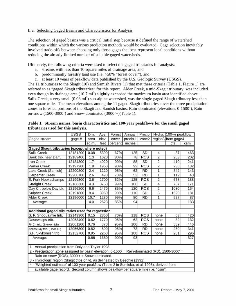
II a. Selecting Gaged Basins and Characteristics for Analysis The selection of gaged basins was a critical initial step because it defined the range of watershed conditions within which the various prediction methods would be evaluated. Gage selection inevitably involved trade-offs between choosing only those gages that best represent local conditions without reducing the already-limited number of suitable gaged watersheds. Ultimately, the following criteria were used to select the gaged tributaries for analysis:

a. streams with less than 10 square miles of drainage area, and b. predominantly forestry land use (i.e. >50% “forest cover”), and c. at least 10 years of peakflow data published by the U.S. Geologic Survey (USGS).

The 11 tributaries to the Skagit (10) and Samish Rivers (1) that met these criteria (Table 1, Figure 1) are referred to as “gaged Skagit tributaries” for this report. Alder Creek, a mid-Skagit tributary, was included even though its drainage area (10.7 mi2) slightly exceeded the maximum basin area identified above. Salix Creek, a very small (0.08 mi2) sub-alpine watershed, was the single gaged Skagit tributary less than one square mile. The mean elevations among the 11 gaged Skagit tributaries cover the three precipitation zones in forested portions of the Skagit and Samish basins: Rain-dominated (elevations 0-1500’), Rain-on-snow (1500-3000’) and Snow-dominated (3000’+)(Table 1). Table 1. Stream names, basin characteristics and 100-year peakflows for the small gaged tributaries used for this analysis.

USGS Drn. Ave. Forest Annual Precip. Hydro. 100-yr peakflowGaged stream gage # area elev. cover precip.1 zone2 region3 from gage4

sq.mi. feet percent inches cfs csmGaged Skagit tributaries (except where noted)Salix Creek 12181200 0.08 5390 67% 125 SD 4 37 463Sauk trib. near Darr. 12189400 1.3 1620 80% 78 ROS 2 263 202Iron Creek 12184300 1.7 4020 99% 88 SD 2 410 241Parker Creek 12197200 1.8 1950 90% 92 ROS 2 238 132Lake Creek (Samish) 12200800 2.4 1220 95% 62 RD 1 342 143Carpenter Creek 12200700 2.6 490 70% 52 RD 1 112 43E. Fork Nookachamps 12199800 3.6 2700 62% 125 ROS 2 678 188Straight Creek 12188300 4.3 3750 99% 106 SD 4 737 171Day Cr. below Day Lk. 12196200 6.6 2470 85% 120 ROS 2 1080 164Sulpher Creek 12191800 8.4 3960 90% 110 SD 3 1520 181Alder Creek 12196000 10.7 1280 99% 80 RD 1 927 87 Average: 4.0 2623 85% 94 183

Additional gaged tributaries used for regressionS. F. Snoqualmie trib. 12143300 0.15 2850 70% 118 ROS none 63 420Dosewalips trib. 12053400 0.62 1770 95% 62 ROS none 82 132Fir Cr. trib. (Skokomish) 12061200 0.76 870 95% 106 RD none 339 446Annas Bay trib. (Hood C.) 12056300 0.82 500 95% 72 RD none 280 341S.F. Skykomish trib. 12132700 0.95 2260 95% 108 ROS none 281 296 Average: 0.66 1650 90% 93 327

1 - Annual precipitation from Daly and Taylor 1998. 2 - Precipitation Zone assigned by basin elevation: 0-1500' = Rain-dominated (RD), 1500-3000' = Rain-on-snow (ROS), 3000'+ = Snow dominated. 3 - Hydrologic region (Skagit tribs only), as delineated by Beechie (1992). 4 - "Weighted estimate" of 100-year peakflow (Table 2 in Sumioka, et al. 1998), derived from available gage record. Second column shows peakflow per square mile (i.e. "csm").

Peakflows for small Skagit tributaries 2 Final Report – May 7, 2001

Figure 1. The locations of small gaged tributaries within the Skagit and Samish basins used in the

Peakflows for small Skagit tributaries 2 Final Report – May 7, 2001

analysis of peakflow prediction methods.

R. 3 E. 4 5 6 7 8 9 10 11 12 13 R. 14 E.

T. 37 N.

36

35

34

33

32

31

30

T. 29 N.

#Y

#Y

#Y

MountVernon

Concrete

Darrington

%U

%U

%U%U

%U

%U%U

%U

%U

#

%U

%U

1

#

Carpenter Creek

#

Lake Creek

#

Parker Cr.

#

AlderCreek

#

DayCreek

#

Sauk trib.

#

Iron Cr.

#

Salix Cr.

#

Straight Cr.

#

SulphurCreek

#

E. Fk. Nooka-champs

N6 0 6 12 18 24 Miles

The scarcity of gaged Skagit tributaries with drainage areas less than one square mile was a key data limitation toward the development of a new prediction equation. To provide additional gaged basins for regression analysis, we identified nine additional USGS gaged basins of less than one square mile that meet the criteria for gage record and forest cover. Although four of these were rejected because their annual precipitation was near the lower limit for forested portions of the Skagit basin (i.e. ~40”), the remaining five fall within the precipitation range (62-118”). These five additional basins, termed “additional gaged basins” for this report, are located in parts of the Puget Sound and Hood Canal drainages with generally similar climate and terrain to the Skagit basin. The five additional gaged basins were included in the development of the new prediction equation, but were not used for evaluating prediction methods because they are located outside the Skagit and Samish basins. The analyses used the 100-year peakflow estimates and watershed characteristics (e.g. drainage area, elevation, forest cover, etc.) published by the USGS (Sumioka et al. 1998), with the exception of average annual precipitation (Table 1), as discussed below. Because the gaged tributaries had 12 - 38 years of record, 100-year peakflow values had been calculated by the USGS from the available annual peaks (see Sumioka et al. 1998 for details). We used the “weighted” peakflow values, which the USGS considers to “provide better estimates of the true flood discharges than those determined from either the flood-frequency analysis or the regression analysis alone” (Sumioka et al. 1998). Annual precipitation values for each basin (Table 1, Figure 2) came from a relatively new precipitation map (Daly and Taylor 1998). This map was developed from a longer period of record and included additional rainfall stations from mountainous areas relative to the U.S. Weather Bureau precipitation map (1965) used by the USGS. The superiority of this newer precipitation data for the Skagit basin was demonstrated by a cursory comparison between mean annual runoff at gaged tributaries and annual precipitation shown on the two precipitation maps. We found the 1998 precipitation values corresponded more closely with average annual runoff (minus estimated evapo-transpiration losses) than did the 1965 USWS values. II b. Existing Peakflow Estimation Methods Several simple peakflow prediction methods are available for the Skagit and Samish River basins. Previous USGS regional peakflow regression equations for Washington were recently revised to include additional flow data including floods of 1989, 1990 and 1996 (Sumioka et al. 1998). This revision included both redrawing of regional boundaries and recalculation of the regression equations. Regional boundaries were drawn relatively broadly, with the entire Skagit and Samish basins included in “Flood Region 2” with all other gaged rivers and streams draining to Puget Sound, Hood Canal or the Straits of Juan de Fuca. The pooling of data from such a broad array of watersheds raises the question of whether important internal differences within the region were overlooked. Specifically, the question of how well the USGS equation predicts 100-year peakflows for small Skagit tributaries is addressed quantitatively in this report. In contrast, Beechie’s hydrologic analysis (1992) focused on the Skagit basin specifically. It included an analysis of flow data from numerous gages within and near the Skagit basin and a delineation of five “hydrologic regions” with similar flow regimes. For predicting peakflows for small tributaries, Beechie provides a “rapid estimation” approach for 50-year peakflows (the regulatory design standard at that time) that offers single unit-area peakflow rates for each hydrologic region. The 50-year peakflow for an ungaged stream is obtained by simply multiplying the unit-area peakflow value for the appropriate hydrologic region (e.g. 165 cfs/mi2 for Region 1) by the drainage area (in square miles). Despite the relative ease of application, Beechie cautions that: “this method may tend to underestimate the discharge in very small basins because smaller basins tend to have higher discharges per unit area than large

Peakflows for small Skagit tributaries 3 Final Report – May 7, 2001

Peakflows for sma

Figure 2. Map of average annual precipitation (1960-1991) within mid- and lower Skagit basin

40 50

60

50 90

140

130

130

100

80

110

60

100

60

70

110

90

60

70

90

70

110

90 140

110

170

90

110

130

110 140 150

160

120

120

90

90

70

90

70

100

80

120

80

R. 3 E. 4 5 6 7 8 9 10 11 12 13 R. 14 E.

T. 37 N.

36

35

34

33

32

31

30

T. 29 N.

#Y

#Y

#Y

MountVernon

Concrete

Darrington

110

6 0 6 12 18 24 Miles

N

S k a g i t R.

(from Daly and

ll Skagit tributaries 4 Final Report – May 7, 2001

Taylor 1998).

basins”. Indeed the tendency for basins less than one square mile to produce larger unit-area peakflows is evident among the 16 gaged tributaries chosen for analysis (Figure 3, Table 1). The sharp increase in unit-area runoff from very small basins has potentially serious consequences, since it could contribute to undersizing of drainage structures on small streams thus making them more likely to fail. Although regression methods provide slightly more sophisticated means of estimating 100-year peakflows for very small basins, Beechie’s analysis provides a valuable characterization of overall flow regimes for larger streams and rivers throughout the Skagit basin.

igure 3. Peakflows (100-year) for gaged Skagit tributaries (solid squares) and additional gaged

f additional concern is that both USGS (Sumioka et al. 1998) and Beechie’s (1992) peakflow methods

c. Developing a New Peakflow Regression Method

0

100

200

300

400

500

600

0 1 2 3 4 5 6 7 8 9 10 11 12

Drainage Area (sq. mi.)

Uni

t are

a 10

0-ye

ar p

eakf

low

(cfs

/sq.

mi.)

Gaged Skagit tributaries

Additional gaged tributaries

trend line - fitted by eye

Fbasins (open squares) used in this analysis expressed on a per-unit-area basis. Note that unit-areapeakflow rates are substantially larger for basins of less than one square mile than for larger basins. Owere developed using streamflow data that included mainstem rivers and major tributaries likely to respond differently to moisture inputs than the small forested tributaries of primary concern. Amongother differences, larger river basins include larger portions of non-forestry land uses (i.e. urban and agriculture) that typically result in more severe hydrologic alteration (e.g. draining, diking, extensive impervious surfaces, etc.). II

o circumvent these concerns, a new prediction equation was developed using only data from small, ysis.

separate regressions for sub-regions within the Skagit basin.

Tforested basins. Both the gaged Skagit tributaries and additional tributaries were included in this analThe limited availability and distribution of small (<10 mi.2), gaged tributaries was insufficient to develop

Peakflows for small Skagit tributaries 5 Final Report – May 7, 2001

The decision to include data from additional small basins located outside the Skagit and Samish basins, a deviation from the initial intent to use only local data, was based on several considerations. In addition to

ose

n

that basin area and annual precipitation were two basin attributes that rovided the greatest predictive value for 100-year peakflows. Both predictive variables and the response

a

AP

where: feet p second, DA = drainage area in square miles, and

II d. Evaluating Peakflo

expanding the sample size, the additional gaged tributaries greatly expand the representation of basins less than one square mile. This presumably results in a predictive relationship that is better supported by data from across the full range of basin sizes for which the method is to be applied. An important observation from the additional tributaries was that the strikingly high unit area discharge for Salix Creek (463 cfs per mi.2), the single gaged Skagit tributary less than one square mile, is fairly similar to thfrom other tributaries of similar basin size, which span a wide range of elevations (Figure 3, Table 2). If the regression had been developed from Skagit tributaries only, the lower end of the resulting regressioline would have been largely determined by tributaries larger than one square mile, which comprise 10 ofthe 11 gaged Skagit tributaries. Our analysis, as elsewhere, foundpvariable (100-year peakflow) were log-transformed for least-squares regression analysis. A review of theranges of input values and the regression results indicated that all statistical assumptions were adequately met (Appendix 2). The resulting two-variable regression equation explains a large part of the variation in 100-year peakflows among the 16 small basins (adjusted r2 = 0.88), and was judged to be highly significant on the basis of the large F statistic (Appendix 2). After conversion from the log-transformed format, the prediction equation is in the form of a power function that responds to input values in curvilinear form and passes through the origin:

Q100 = 0.844 * DA 0.739 * 1.229

Q100 = 100-year peakflow in cubic er

AP = annual precipitation in area inches

w Predictions Against Gage-based Values The utility of the three prediction methods was evaluated based on the similarity between gage-derived

00-year peakflows and peakflow estimates from: 1. Beechie’s (1992) “rapid estimation method”, the

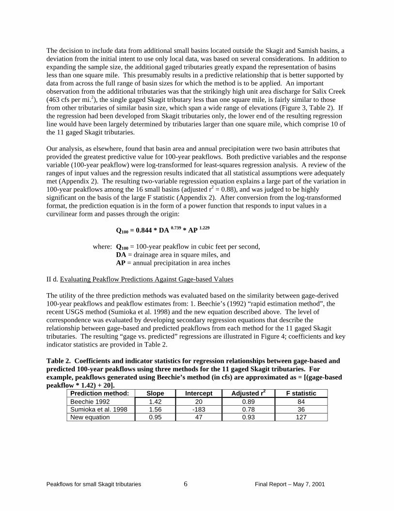
git ts and key

cs for regression relationships between gage-based and redicted 100-year peakflows using three methods for the 11 gaged Skagit tributaries. For

1recent USGS method (Sumioka et al. 1998) and the new equation described above. The level of correspondence was evaluated by developing secondary regression equations that describe the relationship between gage-based and predicted peakflows from each method for the 11 gaged Skatributaries. The resulting “gage vs. predicted” regressions are illustrated in Figure 4; coefficienindicator statistics are provided in Table 2. Table 2. Coefficients and indicator statistipexample, peakflows generated using Beechie’s method (in cfs) are approximated as = [(gage-based peakflow * 1.42) + 20].

Prediction method: Slope Intercept Adjusted r2 F statistic Beechie 1992 1.42 20 0.89 84 Sumioka et al. 1998 1.56 -183 0.78 36 New equation 0.95 47 0.93 127

Peakflows for small Skagit tributaries 6 Final Report – May 7, 2001

0

500

1000

1500

2000

2500

3000

0 500 1000 1500 2000 2500 3000

Peakflow from gage record (cfs)

Pred

icte

d pe

akflo

w (c

fs)

Beechie 1992

Sumioka et al. 1998

New equation

1:1 line

Figure 4. Correlation between gage-generated peakflows (100-year) and peakflows predicted using three alternative methods. Point markers indicate peakflow values for each of the 11 gaged Skagit tributaries; lines are best-fit regressions between gage-generated and predicted peakflows (regression coefficients are shown in Table 3). The relative “accuracy” of each prediction method was evaluated on the basis of the slope coefficient, while the “precision” was indicated by the adjusted r2. The optimal value for both statistics is 1.0. Gomez and Church (1989) used a similar approach for evaluating predictive equations for bed load sediment transport. On the basis of these two regression statistics (Table 2), the new prediction equation was judged both more accurate and precise than either of the two pre-existing methods. In particular, the slope coefficient for the new equation (i.e. 0.95) suggests considerably higher accuracy than do the slopes for the two pre-existing methods (i.e. 1.42 and 1.56), both of which suggest a general tendency to overpredict actual flows. The tendency for each method to over or under-predict peakflows for ungaged streams is of considerable practical interest to those using peakflow predictions for design use. For this reason, the magnitude and direction of the percent differences between gage-generated and predicted peakflows were inspected for each method among the 11 gaged Skagit tributaries (Table 3). The distribution of gage-by-gage differences produced using each method is illustrated in the histogram in Figure 5. Thirty percent was chosen as the break-off for the smallest bin because it represents the approximate increase in hydraulic capacity gained by a six-inch increase in culvert diameter. Therefore, peakflow estimates that deviate from the actual value by less than 30% are likely to result in a culvert diameter within one standard culvert size increment of the optimal size. from the actual value by less than 30% are likely to result in a culvert diameter within one standard culvert size increment of the optimal size. We note that Beechie’s “rapid estimates” exceeded the 100-year peakflows for all but two gaged tributaries, including six where over-predictions exceeded 30% (Figure 5). This tendency to over-predict 100-year peakflows was surprising since Beechie’s method was developed to predict 50-year peakflows, which are typically 10-20% smaller. Interestingly, the one basin for which Beechie’s method

We note that Beechie’s “rapid estimates” exceeded the 100-year peakflows for all but two gaged tributaries, including six where over-predictions exceeded 30% (Figure 5). This tendency to over-predict 100-year peakflows was surprising since Beechie’s method was developed to predict 50-year peakflows, which are typically 10-20% smaller. Interestingly, the one basin for which Beechie’s method

Peakflows for small Skagit tributaries 7 Final Report – May 7, 2001

Table 4. Peakflows from gage data at gaged tributaries and from prediction equations. Drn. Ave. 100-year peakflows:

Gaged stream area elev. from gage1 pred.-Beechie2 pred.-Sumioka3 pred.-newsq.mi. feet cfs csm cfs % dif.4 cfs % dif.4 cfs % dif.4

Gaged Skagit tributaries (except where noted)Salix Creek 0.08 5390 37 463 14 -63% 66 79% 49 33%Sauk tributary 1.3 1620 263 202 332 26% 259 -2% 217 -18%Iron Creek 1.7 4020 410 241 434 6% 477 16% 306 -25%Parker Creek 1.8 1950 238 132 459 93% 219 -8% 338 42%Lake Creek 2.4 1220 342 143 396 16% 196 -43% 257 -25%Carpenter Creek 2.6 490 112 43 429 283% 126 12% 220 96%E.Nookachamps 3.6 2700 678 188 918 35% 398 -41% 821 21%Straight Creek 4.3 3750 737 171 731 -1% 1524 107% 765 4%Day Creek 6.6 2470 1080 164 1683 56% 963 -11% 1223 13%Sulpher Creek 8.4 3960 1520 181 2058 35% 2712 78% 1313 -14%Alder Creek 10.7 1280 927 87 1766 90% 963 4% 1062 15% Average: 4.0 2623 183 64% 32% 27%

Additional gaged tributaries used for regressionS.F. Snoq. trib. 0.15 2850 63 420 none ----- 80 28% 73 16%Dosewalips trib. 0.62 1770 82 132 none ----- 88 7% 95 15%Fir Cr. trib. 0.76 870 339 446 none ----- 279 -18% 213 -37%Annas Bay trib. 0.82 500 280 341 none ----- 170 -39% 140 -50%S.F. Sky. trib. 0.95 2260 281 296 none ----- 275 -2% 256 -9% Average: 0.66 1650 327 31% 28%

1 - "Weighted estimate" of 100-year peakflow (Table 2 in Sumioka, et al. 1998), derived from available gage record. Second column shows peakflow per square mile (i.e. "csm"). 2 - Peakflow estimate (50-year, Skagit tribs only) from Beechie's (1992) "rapid estimation" method. 3 - Peakflow estimate (100-year) from Sumioka et al. 1998. 4 - Difference between predicted peakflow and gage-derived peakflow. underpredicted substantially was Salix Creek, the smallest gaged Skagit tributary. This tends to confirm Beechie’s caveat that his method could underestimate peakflows for very small basins. As shown in Figure 5, peakflow estimates from the USGS method (Sumioka, et al. 1998) were generally closer to gage-derived values than were Beechie’s. Under- and over-predictions were fairly balanced (Figure 5), though the three largest percent differences (+78%, +79% & +107%) were all over-predictions (Table 2). It should be noted that the USGS estimates were calculated using annual precipitation values from the 1965 US Weather Bureau map, which indicates less precipitation for most forest lands in the Skagit basin relative to the more recent map (Daly and Taylor 1998). To see if inaccurate precipitation values were reducing the accuracy of the USGS method, we recalculated USGS estimates using 1998 precipitation values, but found that this resulted in less accurate peakflow estimates than using the 1965 data. The fact that the new prediction equation estimated peakflows fairly well should not be terribly surprising, since it was developed from these data specifically. Similar to the results of the USGS method, all three differences that exceeded 30% were over-predictions. Only one gaged Skagit tributary--Carpenter Creek--was overestimated by more than 42% (i.e. +96%, see Table 3). None of the 11 gaged Skagit tributaries were under-predicted by more than 30% (Figure 4), though two of the very small additional basins were (Table 3). Significantly, the new equation provides the best overall representation of peakflows among the six basins smaller than one square mile (Table 5).

Peakflows for small Skagit tributaries 8 Final Report – May 7, 2001

0

1

2

3

4

5

+ 100+% + 31-100% + 0-30% - 0-30% - 31-100% - 100+%

Difference between estimated and gage-based peakflow

Gag

ed S

kagi

t trib

utar

ies

(#)

6

Beechie 1992

Sumioka et al. 1998

New equation

peakflow overpredicted peakflow underpredicted

Figure 5. Distribution of the percent difference between peakflow estimates using three local thods and gage-derived values for 11 gaged Skagit tributaries. me

all quantitative standards, an dditional advantage is that it was fitted to the updated precipitation data (Figure 2), which appears to etter represent precipitation differences across the Skagit basin. For these reasons, we recommend the

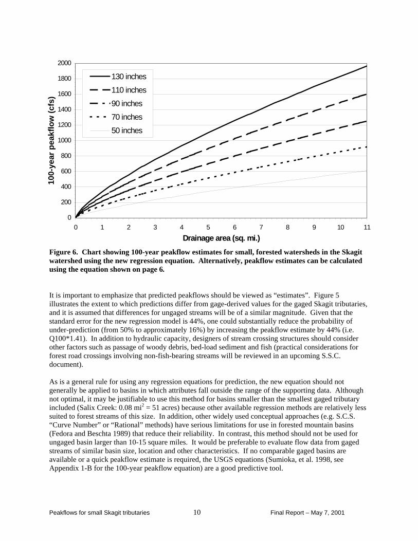
Although the new equation provided the best peakflow predictions by abnew equation for use in small, ungaged forested basins. II e. Guidance for Applying the New Peakflow Equation Using the new equation to calculate a 100-year peakflow estimate for an ungaged basin requires

nnual precipitation should be determined by cating the basin on the precipitation map in Figure 2 or by using local data, if available. Figure 2 is a

n can 1

r basins where the precipitation

te is intermediate between values plotted on Figure 6, one can interpolate along the vertical distance between curves using a ruler.

determining the drainage area and annual precipitation. Alosimplified representation; a larger (statewide) and more finely resolved (2” isohyets) representatiobe acquired from the web-site or from the authors of this report. Using annual precipitation values fromthe widely available US Weather Bureau (1965) is likely to produce less accurate estimates. An accuratevalue for basin area can be surprisingly difficult to determine, especially for basins that are very small (<mi2) and/or poorly defined topographically. Although basin delineation on a topographic map is the standard and easiest method, our experience suggests that stereo inspection of air photos (or even ground checking) is frequently necessary to avoid sizable misinterpretations. Once drainage area and annual precipitation are known, you can calculate the peakflow estimate using theequation on page 6 or graphically using the chart in Figure 6, below. Fora

Peakflows for small Skagit tributaries 9 Final Report – May 7, 2001

0

200

400

600

800

1000

1200

1400

1600

1800

0 1 2 3 4 5 6 7 8 9 10 11

Drainage area (sq. mi.)

100-

year

pea

kflo

w (c

fs)

2000

130 inches

110 inches

90 inches

70 inches

50 inches

Figure 6. Chart showing 100-year peakflow estimates for small, forested watersheds in the Skagit watershed using the new regression equation. Alternatively, peakflow estimates can be calculated using the equation shown on page 6. It is important to emphasize that predicted peakflows should be viewed as “estimates”. Figure 5 illustrates the extent to which predictions differ from gage-derived values for the gaged Skagit tributariesand it is assumed that differences for un

, gaged streams will be of a similar magnitude. Given that the

tandard error for the new regression model is 44%, one could substantially reduce the probability of nder-prediction (from 50% to approximately 16%) by increasing the peakflow estimate by 44% (i.e.

sider

utary lix Creek: 0.08 mi = 51 acres) because other available regression methods are relatively less

uited to forest streams of this size. In addition, other widely used conceptual approaches (e.g. S.C.S. ns

suQ100*1.41). In addition to hydraulic capacity, designers of stream crossing structures should conother factors such as passage of woody debris, bed-load sediment and fish (practical considerations for forest road crossings involving non-fish-bearing streams will be reviewed in an upcoming S.S.C. document). As is a general rule for using any regression equations for prediction, the new equation should not generally be applied to basins in which attributes fall outside the range of the supporting data. Although not optimal, it may be justifiable to use this method for basins smaller than the smallest gaged tribincluded (Sa 2

s“Curve Number” or “Rational” methods) have serious limitations for use in forested mountain basi(Fedora and Beschta 1989) that reduce their reliability. In contrast, this method should not be used for ungaged basin larger than 10-15 square miles. It would be preferable to evaluate flow data from gaged streams of similar basin size, location and other characteristics. If no comparable gaged basins are available or a quick peakflow estimate is required, the USGS equations (Sumioka, et al. 1998, see Appendix 1-B for the 100-year peakflow equation) are a good predictive tool.

Peakflows for small Skagit tributaries 10 Final Report – May 7, 2001

III. Acknowledgements We appreciate Doug Couvelier’s help with of the precipitation map in Figure 2. Thanks to the following for review comments: Tim Beechie (N.M.F.S.), Jeff Grizzel and Noel Wolff (Washington D.N.R.), Keith Wyman, Doug Couvelier and John Klochak (S.S.C.). IV. References Beechie, T. J. 1992. Delineation of hydrologic regions in the Skagit River Basin. Skagit System

Cooperative, LaConner, Washington. Daly, C. and G. Taylor. 1961-90 Mean annual precipitation maps for the coterminous United States.

Isohyetal map available via internet from the Western Regional Climate Data Center, Corvallis, Oregon.

Dunne, T., and L. B. Leopold. 1978. Water in Environmental Planning. W. H. Freeman and Company,

New York, N.Y. Fedora, M.A. and R. L. Beschta. 1989. Storm runoff simulation using an antecedent precipitation index

(API) model. Journal of Hydrology. 112:121-133. Furniss, M. J., T. S. Ledwith, M. A. Love, B. C. McFadin and S. A. Flanagan. 1998. Response of road-

stream crossings to large flood events in Washington, Oregon and northern California. Publication 9877-1806, USDA Forest Service Technology and Development Program, San Dimas Technology and Development Center, California.

Gomez, B. and M. Church. 1989. An assessment of bed load sediment transport formulae for gravel bed

rivers. Water Resources Research, 25 (6): 1161-1186. Hayman, R. A., E. M. Beemer, T. Beechie, K. Wyman and S. Fransen. 1991. November 1990: a

preliminary assessment of flood damage to the Skagit River fisheries resources. Internal report prepared by Skagit System Cooperative, LaConner, Washington.

Sumioka, S.S., D. L. Kresch and K. D. Kasnick. 1998. Magnitude and frequency of floods in

Washington. USGS Water-Resources Investigations Report 97-4277 (on-line version). Denver, Colorado.

United States Weather Bureau. 1965. Mean Annual precipitation in Washington, 1930-57.

Peakflows for small Skagit tributaries 11 Final Report – May 7, 2001

APPENDIX 1. Summaries of Beechie’s (1992) “Rapid Estimation” Method and USGS Regional Equation (Sumioka et al. 1998) for 100-year peakflows

irst determine hydrologic region and drainage area (in square miles) of stream. To calculate the 50-year eakflow, multiply the drainage area by the unit area peakflow for hydrologic region shown in the

chie advises: “If the drainage basin is near a boundary between two hydrologic regions, ou may want to interpolate between the estimates of QPF50 (i.e. the unit area 50-year peakflows) for the

(see Beechie 1992 for locations)

(cfs per mile2)

A. Beechie’s (1992) “Rapid estimation of 50-year peak flows” Fptablebelow. Beeyadjoining regions”

Hydrologic Region

Unit area 50-year peakflow

1 165

2 255

3 245

4 170

5 80

S Regional Equation (Sumioka et al. 1998)

. USG

uget S rediction equations for the peakflows ictive

annual

wing

Q100 = 0.174 * DA 0.861 * AP 1.62

DA = drainage area in square miles, and AP = annual precipitation in inches

B The entire Skagit and Samish basins are within Flood Region 2, which includes all drainages entering

ound, Hood Canal and the Straits of Juan de Fuca. The pPrequire both the drainage area (in square miles) and average annual precipitation (in inches) as predvariables. Because the equation was developed using precipitation values from the 1965 USWS map of

precipitation, it is advisable to use the same data source for the basin being evaluated. From these attributes, the 100-year peakflow estimate (Q100 in cfs) is determined using the folloequation:

where: Q100 = 100-year peakflow in cubic feet per second,

Peakflows for small Skagit tributaries i Final Report – May 7, 2001

Input data (drainage area, annual precipitation and 100-year peakflows, all log-transformed) were

one of the three data sets showed erious deviations from normality. All three histograms and associated statistical indicators (generated

0-year discharge (bottom).

0

APPENDIX 2. Statistical Evaluation of Skagit Peakflow Regression Analysis

analyzed for normality using histograms and summary statistics. Nsusing the “Eviews” statistics software) are shown below (Figures A1, 2 & 3). Figure 1. Histograms and indicator statistics for annual precipitation (top), drainage area (middle) and gage-based 10

1

2

3

4

5

-1 0 -0 5 0 0 0 5 1 0

Series: DASample 1 16Observations 16

Mean 0.187609Median 0.242861Maximum 1.029384Minimum -1.096910Std. Dev. 0.584720Skewness -0.643549K 2.937264

Jarque-Bera 1.107038Probability 0.574923

Log Drainage Area (square miles)

urtosis

Log Annual Precipitation (inches)

0

1

2

3

4

5

1 70 1 75 1 80 1 85 1 90 1 95 2 00 2 05 2 10

Series: APSample 1 16Observations 16

Mean 1.958243Median 1.994547Maximum 2.096910Minimum 1.716003Std. Dev. 0.120850

Jarque-Bera 1.399448robability 0.496722

Skewness -0.571645Kurtosis 2.110022

P

Log Discharge (cfs)

0

1

2

3

4

5

1 50 1 75 2 00 2 25 2 50 2 75 3 00 3 25

Series: QSample 1 16Observations 16

Mean 2.472306Median 2.489453Maximum 3.181844Minimum 1.544068Std. Dev. 0.461410Skewness -0.413117Kurtosis 2.401692

Jarque-Bera 0.693757Probability 0.706891

Peakflows for small Skagit tributaries ii Final Report – May 7, 2001

lightly skewed, the arque-Bera (JB) statistic used to test for normality is 1.39. Whenever this statistic is less than 5.991, it

a is

tribution of the response

ariable (i.e. discharge, see Figure A3) was also examined and found to be very close to normal. kewness, Kurtosis, and JB statistics all suggest that it is reasonable to treat these populations as normally

curately reflect the value of the input data and predictive model. Table A below documents the results and statistics associated with the resulting regression model. Both input variables were found to have significant predictive value (p>.95). The relatively high F-statistic (56.6) suggests that the regression model as a whole is valuable in predicting the response variable, 100-year discharge. Table A. Statistical indicator values for the regression model that predicts 100-year peakflow on the basis of annual precipitation and drainage area. Table reproduced from output from the Eviews statistical software.

s a final test, the Durbin-Watson statistic was used to test for autocorrelation in the dataset. his is a standard test for randomness in the residuals of regression predictions relative to actual response

values. Because the Durban-Watson statistic (Wstat = 1.719) is higher than the upper bound value (DU=1.54), the residuals are considered random and the t and F statistics are not considered biased. Based on the analysis above, no statistical problems were identified in predicting 100-year peak discharge from drainage area and annual precipitation within the range of the input data. There were no serious deviations from normality in the underlying dataset, and the regression was found to be valuable in the prediction of discharge.

Dependent Variable: Q Method: Least Squares Date: 01/29/01 Time: 12:34 Sample: 1 16 Included observations: 16

Variable Coefficient Std. Error t-Statistic Prob.

While the histogram for log-transformed annual precipitation (Figure A1) appears sJsuggests that the series is normal. The slight kurtosis in the underlying distribution was not seen asserious deviation from normality. The distribution of the log-transformed drainage areas (Figure A2)almost normal. The skewness value is small, the Kurtosis value very close to three (a value of 3.0 meansno Kurtosis), and the JB statistic is far below the critical value of 5.991. The disvSdistributed. Therefore the t and F statistics for the regression, based on the demonstrated normal distribution of input and output values, should ac

C -0.073426 0.674864 -0.108802 0.9150 DA 0.738840 0.070897 10.42137 0.0000 AP 1.229224 0.343025 3.583479 0.0033

R-squared 0.897066 Mean dependent var 2.472306 Adjusted R-squared 0.881230 S.D. dependent var 0.461410 S.E. of regression 0.159016 Akaike info criterion -0.672263 Sum squared resid 0.328719 Schwarz criterion -0.527403 Log likelihood 8.378107 F-statistic 56.64720 Durbin-Watson stat 1.719198 Prob(F-statistic) 0.000000

AT

Peakflows for small Skagit tributaries iii Final Report – May 7, 2001