Page 1
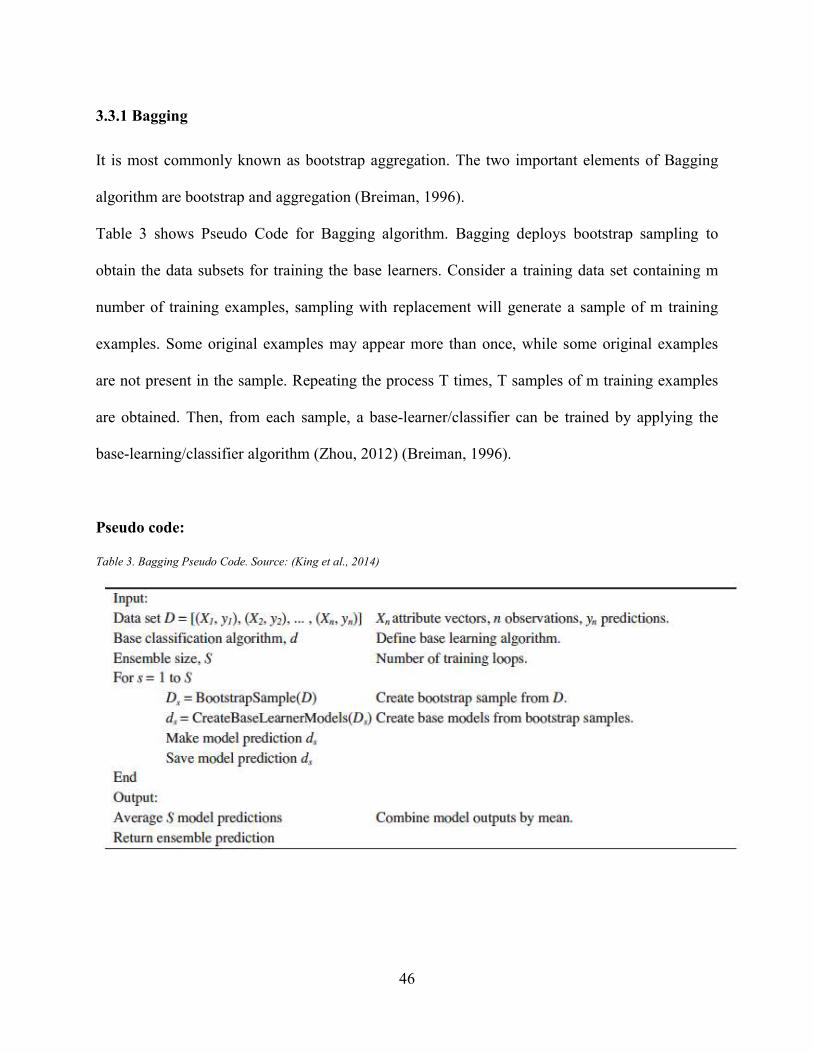
I
Predicting road transport GHG emissions with application for Canada
Mohd Jawad Ur Rehman Khan
A Thesis
in the
Concordia Institute for Information Systems Engineering (CIISE)
Presented in Partial Fulfillment of the Requirements
For the Degree of Master of Applied Science (Quality Systems Engineering) at
Concordia University
Montreal, Quebec, Canada
September 2017
© Mohd Jawad Ur Rehman Khan, 2017
Page 2
II
CONCORDIA UNIVERSITY
School of Graduate Studies
This is to certify that the thesis prepared
By: Mohd Jawad Ur Rehman Khan
Entitled: Predicting road transport GHG emissions with application for Canada
And submitted in partial fulfillment of the requirements for the degree of
Master of Applied Science (Quality Systems Engineering)
Complies with the regulations of the University and meets the accepted standards with
respect to originality and quality.
Signed by the final examining committee:
Dr. Jia Yuan Yu Chair (CIISE)
Dr. Walter Lucia Internal Examiner (CIISE)
Dr. Shannon Llyod External Examiner (JMSB)
Dr. Anjali Awasthi Supervisor (CIISE)
Approved by
Chair of Department or Graduate Program Director
Date Dean of Faculty
Page 3
III
Abstract
Predicting road transport GHG emissions with application for Canada
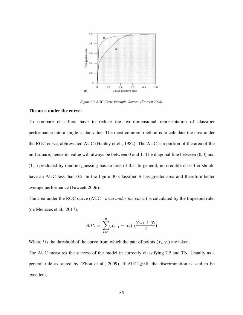
Prediction of greenhouse gas (GHG) emissions is vital to minimize their negative impact on
climate change and global warming. In this thesis, we propose new models based on data mining
and supervised machine learning algorithms (Regression and classification) for predicting GHG
emissions arising from passenger and freight road transport in Canada. Four categories of models
are investigated namely artificial neural network multilayer perceptron, multiple linear
regression, multinomial logistic regression and decision tree models. From the application
results, it was found that artificial neural network multilayer perceptron model showed better
predictive performance over other models. Ensemble technique (Bagging & Boosting) was
applied on the developed Multilayer Perceptron model which significantly improved the model's
predictive performance.
The independent variable importance analysis conducted on multilayer perceptron model
disclosed that among the input attributes Light truck emissions, Car emissions, GDP
transportation, Heavy truck emission, Light duty truck fuel efficiency, Interest rate (overnight),
Medium Trucks Emission, Passenger car fuel efficiency and Gasoline Price have higher
sensitivity on the output of the predictive model of GHG emissions by Canadian road transport.
Scenario analysis is conducted using widely available socioeconomic, emission and fuel
efficiency attributes as inputs in multilayer perceptron (with bagging) model. The results show
that in all Canadian road transport GHG emission projection scenarios, all the way through 2030,
Page 4
IV
emissions from Light trucks will hold a major share of GHG emissions. Thereby, rigorous efforts
should be made in mitigating GHG emissions from these trucks (freight transport) to meet the
ambitious GHG emission target for Canadian road transport.
Page 5
V
Acknowledgements
First and foremost, I would like to thank God who bestowed upon me this wonderful opportunity
to pursue my graduate studies at Concordia University under the supervision of Dr. Anjali
Awasthi and for gifting me the power to be in the place where I am today personally and
professionally.
I would like to acknowledge and extend wholeheartedly my sincere gratitude to my thesis
supervisor Dr. Anjali Awasthi for providing me with immense continuous support, patience,
motivation, and guidance throughout my thesis work. Her wisdom and words of encouragement
encouraged me to perform best in my research work. Further, I would also like to extend my
gratitude wholeheartedly to her for being so compassionate and understanding.
Additionally, I want to thank all the professors of Concordia Institute for Information Systems
Engineering (CIISE) and Concordia University for providing the best knowledge and education
in all the courses, which helped me to advance my knowledge in systems engineering. Also, I
want to thank CIISE’s administrative staffs who never failed to bring a smile on my face, thank
you!
Most importantly, I would like to thank my creators (my parents) and my friends for providing
me with their unconditional love and support in every possible way. Their faith and belief in me
have given me enormous strength and courage to accomplish my goals.
Page 6
VI
Table of Contents
Abstract ........................................................................................................III
Acknowledgements....................................................................................... V
List of Figures .............................................................................................. XI
List of Tables ............................................................................................ XIII
Introduction ................................................................................................... 1
1.1 Background ................................................................................................................... 1
1.1.1 Green House Gases .................................................................................................... 1
1.1.2 Green House Gases Emissions................................................................................... 1
1.1.3 Green House Gases effects ........................................................................................ 3
1.2 Context of Study ........................................................................................................... 3
1.4 Contribution of the Study.............................................................................................. 4
1.3 Thesis Objectives/Thesis Statement ............................................................................. 5
1.5 Thesis Organization ...................................................................................................... 7
Literature Review ......................................................................................... 8
2.1 Methods to Evaluate GHG emissions ........................................................................... 8
2.1.1 Road Transport Emission Inventory Models ............................................................. 9
COPERT ............................................................................................................................. 9
Mobile 6.2 model and Motor Vehicle emission simulator (Moves) ................................. 11
2.2 Other Emission Inventory Models .............................................................................. 12
GAINS (Gas and Air pollution Interactions and synergies) ............................................. 12
Page 7
VII
2.3 Limitations of the models used to evaluate road transport GHG emissions ............... 13
2.4 Research papers .......................................................................................................... 15
2.5 Research Gap .............................................................................................................. 16
Methodologies .............................................................................................. 18
3.1 Feature Selection ......................................................................................................... 18
3.1.1 Relief Attribute Evaluator ........................................................................................ 19
Basic Relief Algorithm ..................................................................................................... 20
RReliefF Algorithm .......................................................................................................... 21
3.2 Data Mining ................................................................................................................ 23
3.2.1 Supervised Learning ................................................................................................ 24
Multiple Linear Regression............................................................................................... 26
Multinomial Logistic Regression ...................................................................................... 29
Multilayer Perceptron ....................................................................................................... 31
Decision trees (ID3 & C4.5) ............................................................................................. 38
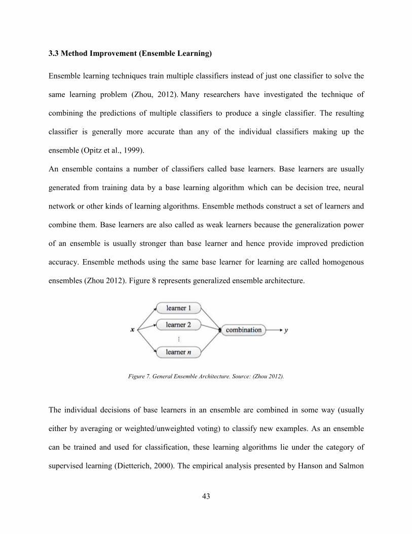
3.3 Method Improvement (Ensemble Learning) ............................................................... 43
3.3.1 Bagging .................................................................................................................... 46
3.3.2 Boosting ................................................................................................................... 47
Research Methodology ............................................................................... 51
Phase 1: GHG Emissions Landscape of Canada ..................................... 53
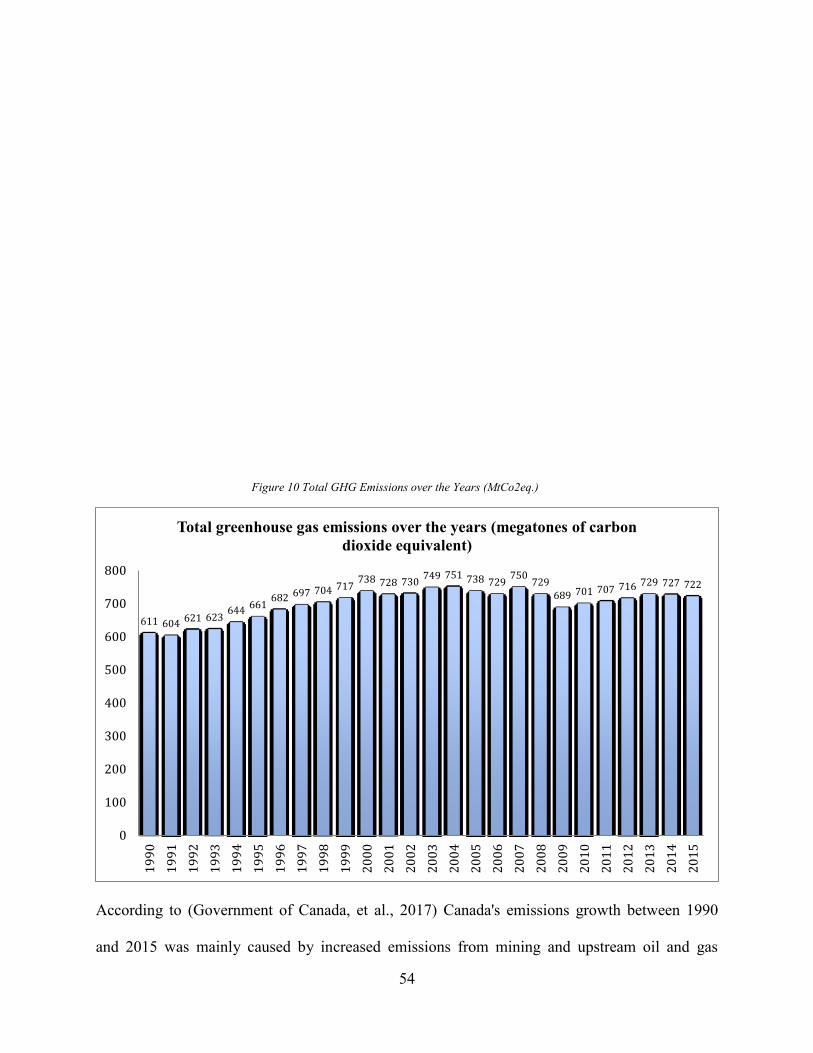
4.1 GHG emissions in Canada .......................................................................................... 53
4.1.1 GHG analysis in Canada .......................................................................................... 55
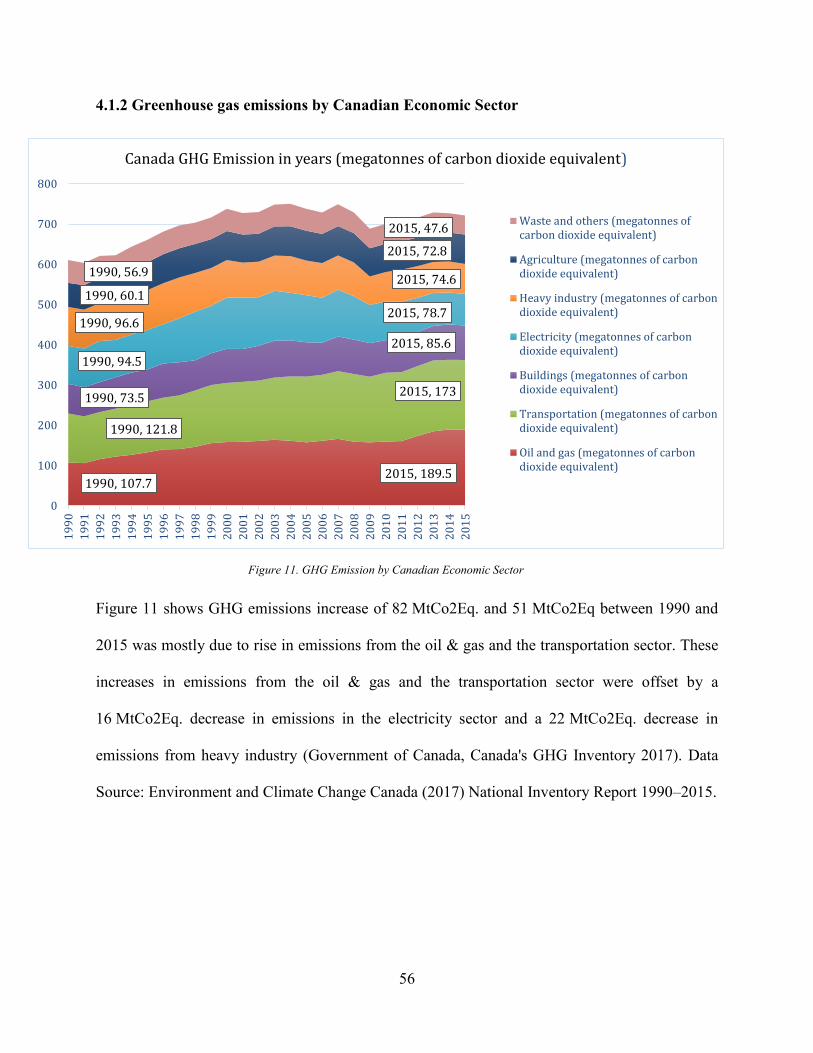
4.1.2 Greenhouse gas emissions by Canadian Economic Sector ...................................... 56
Page 8
VIII
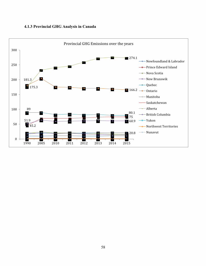
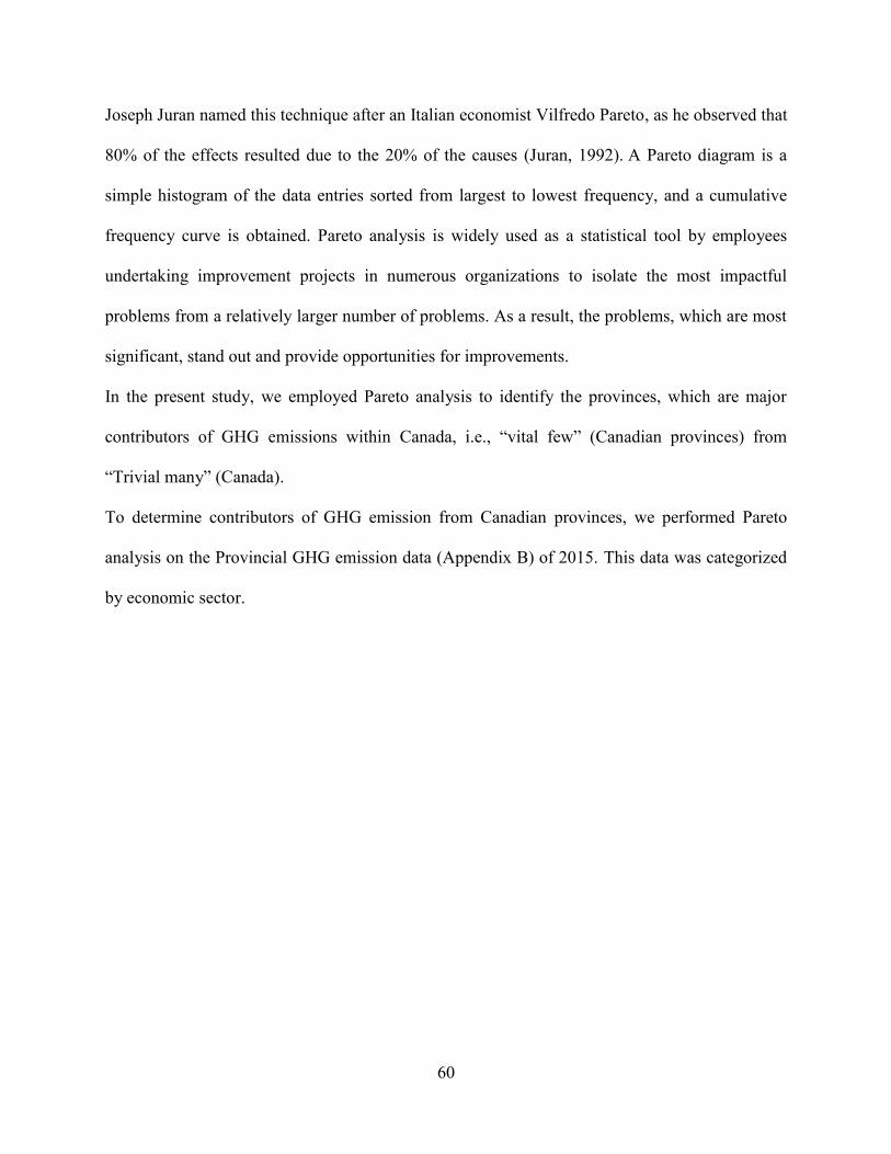
4.1.3 Provincial GHG Analysis in Canada ....................................................................... 58
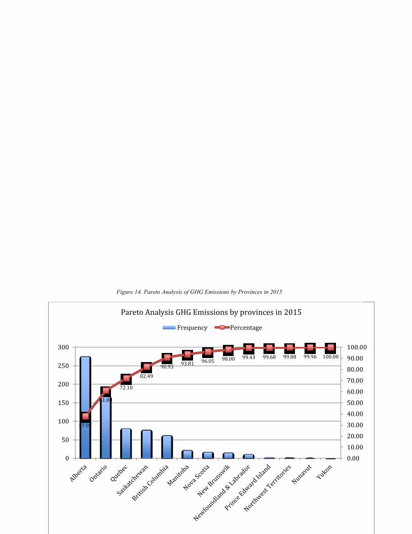
4.1.4 Major GHG Emitting Provinces (GHG Emission Distribution by Economic Sector)62
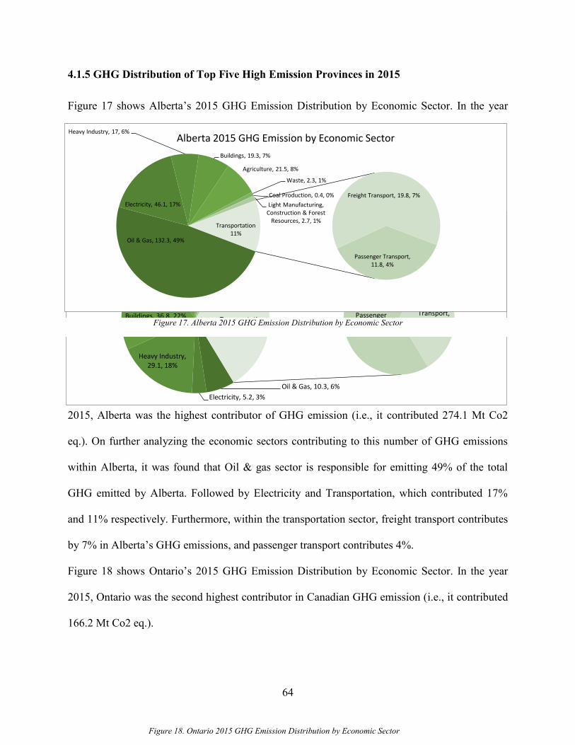
4.1.5 GHG Distribution of Top Five High Emission Provinces in 2015 .......................... 64
4.1.6 GHG emission by Transportation Sector ................................................................. 67
4.1.7 GHG Emission by Road Transport .......................................................................... 70
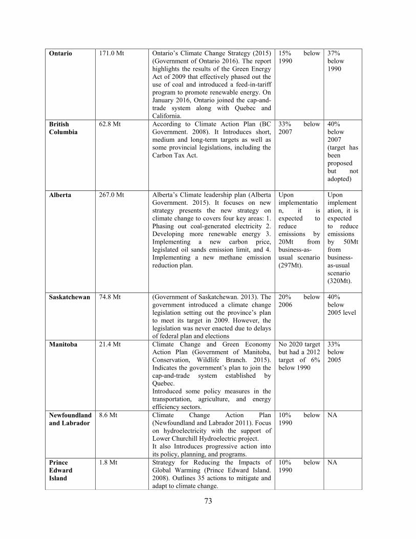
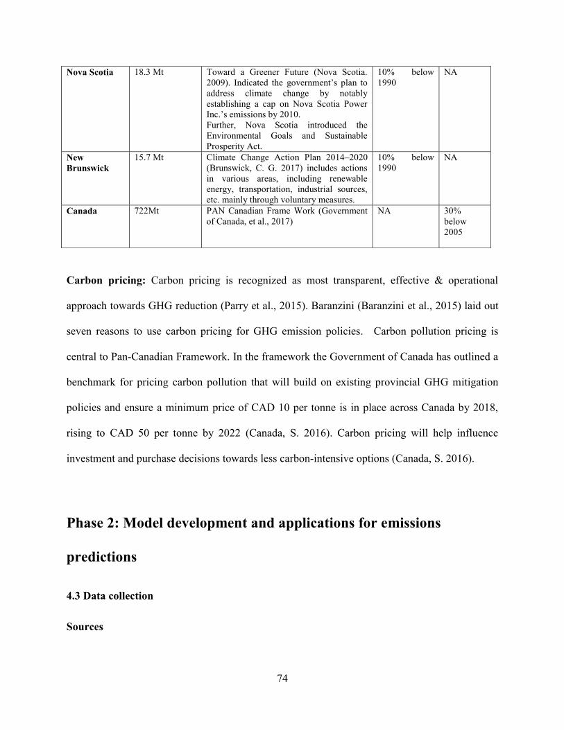
4.2 GHG Mitigation Initiatives in Canada ........................................................................ 71
Phase 2: Model development and applications for emissions predictions74
4.3 Data collection ............................................................................................................ 74
Application ........................................................................................................................ 77
4.4 K-fold cross validation ................................................................................................ 77
4.5 Performance Evaluation Metrics................................................................................. 79
4.6 Attribute selection (Ranking) ...................................................................................... 86
Verification of Selected Attributes ................................................................................... 87
Results of Selected Attribute Verification ........................................................................ 90
4.7 Algorithm Application on Numeric Data ................................................................... 92
Multiple Linear Regression............................................................................................... 92
Multilayer Perceptron ....................................................................................................... 94
4.7.1 Algorithm Improvement for Numeric Data ............................................................. 96
Bagging ............................................................................................................................. 97
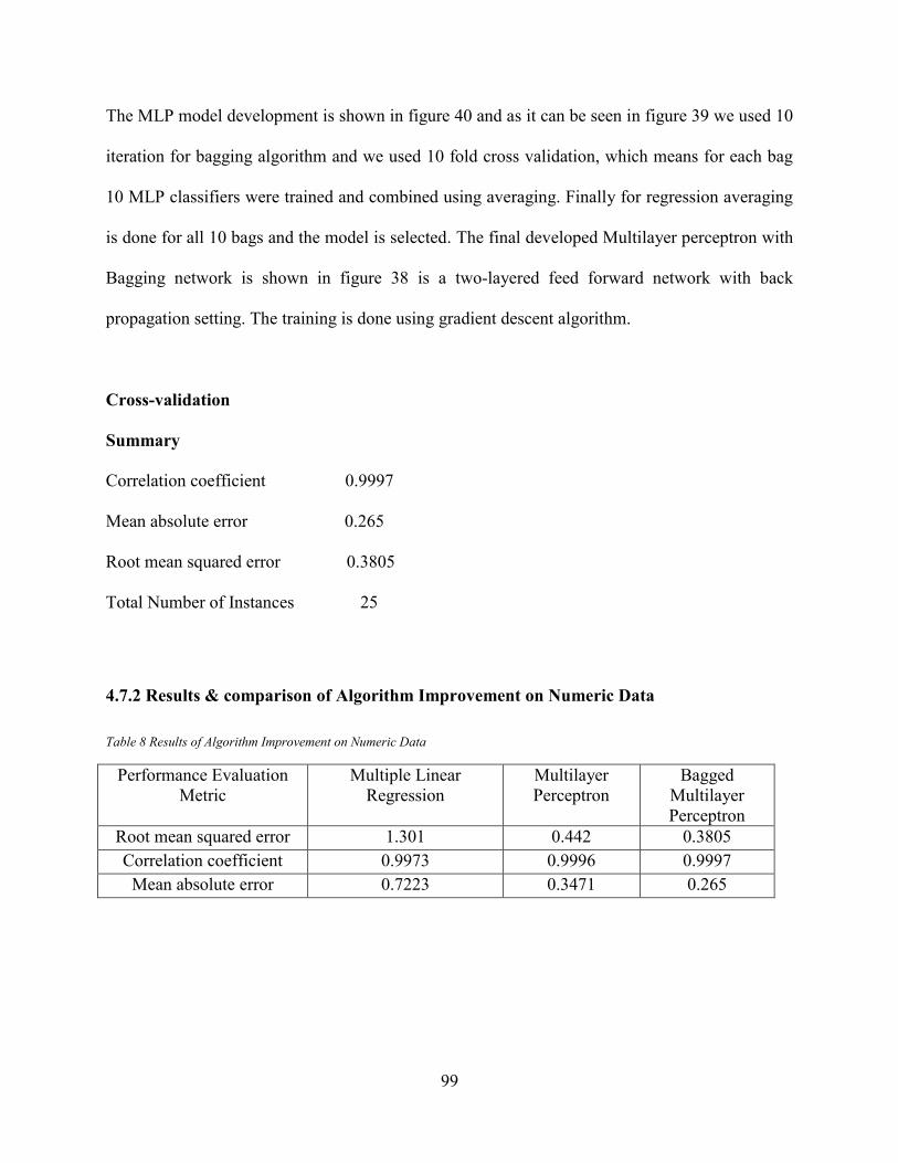
4.7.2 Results & comparison of Algorithm Improvement on Numeric Data ..................... 99
4.8 Algorithm Application on Nominal Data ................................................................. 101
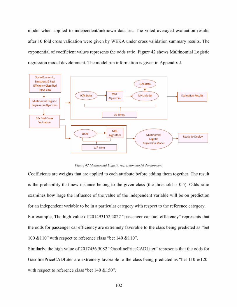
Multinomial Logistic Regression .................................................................................... 101
Decision Tree .................................................................................................................. 104
Page 9
IX
Multilayer Perceptron ..................................................................................................... 107
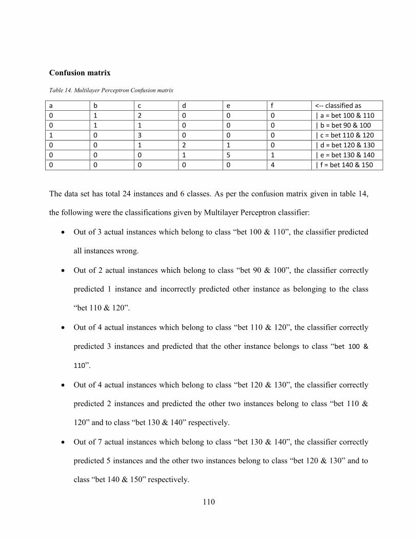
4.8.1 Algorithm Improvement for Nominal Data ........................................................... 111
Bagging ........................................................................................................................... 111
Boosting .......................................................................................................................... 115
4.8.2 Results & comparison of Algorithm Improvement on Nominal Data ................... 119
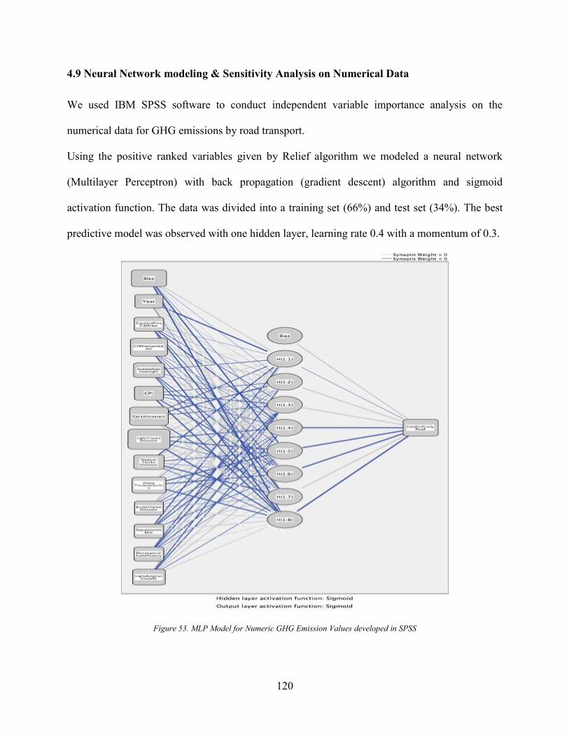
4.9 Neural Network modeling & Sensitivity Analysis on Numerical Data .................... 120
4.9.1 Independent Variable Importance Analysis ........................................................... 122
Phase 3: Canada GHG emissions scenario analysis .............................. 124
4.10 GHG Emission Future Projections and Scenario Analysis ..................................... 124
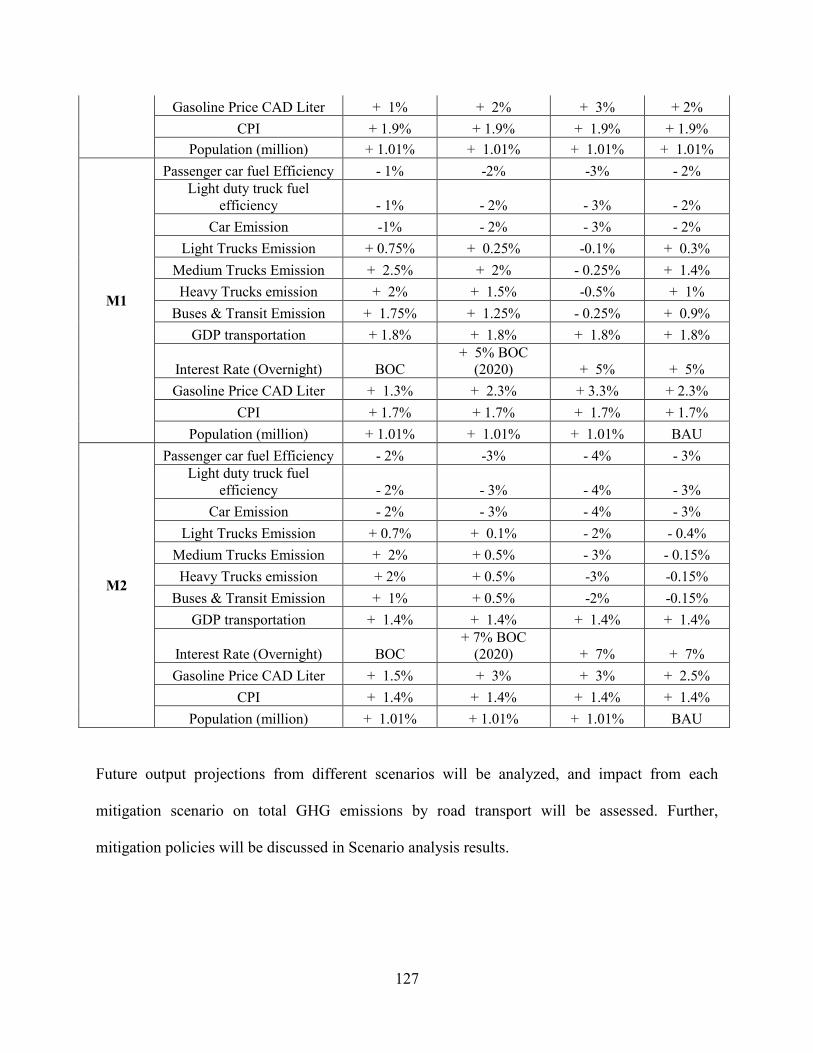
4.11 Scenario Analysis.................................................................................................... 125
4.11.1 Business as Usual Scenario (BAU)...................................................................... 128
4.11.2 Low Emission Scenarios ...................................................................................... 130
Minimum mitigation scenario (M1)................................................................................ 131
Maximum Mitigation Scenario (M2) .............................................................................. 134
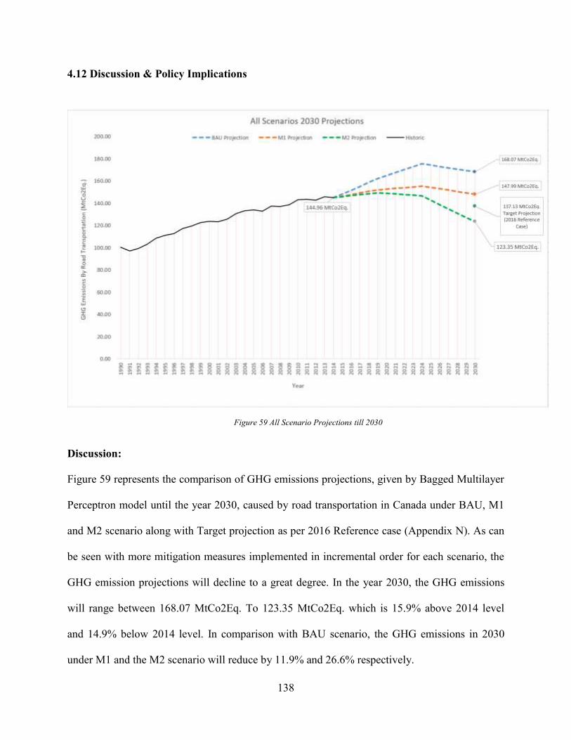
4.12 Discussion & Policy Implications ........................................................................... 138
4.13 Sensitivity Analysis of Model ................................................................................. 141
Conclusion and Future Works ................................................................. 143
References .................................................................................................. 146
Appendices ................................................................................................. 165
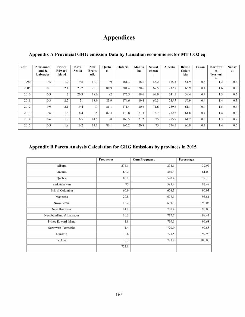
Appendix A Provincial GHG emission Data by Canadian economic sector MT CO2 eq165
Appendix B Pareto Analysis Calculation for GHG Emissions by provinces in 2015 .... 165
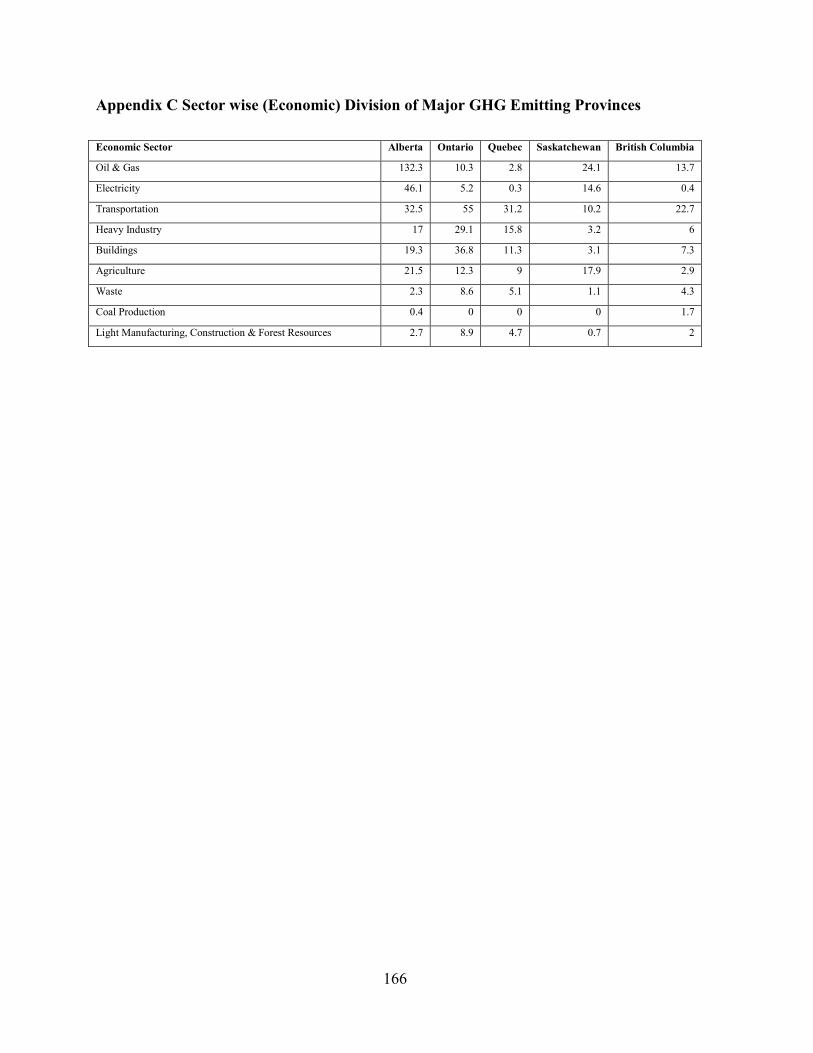
Appendix C Sector wise (Economic) Division of Major GHG Emitting Provinces ...... 166
Page 10
X
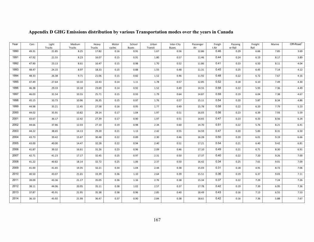
Appendix D GHG Emissions distribution by various Transportation modes over the years in
Canada............................................................................................................................. 167
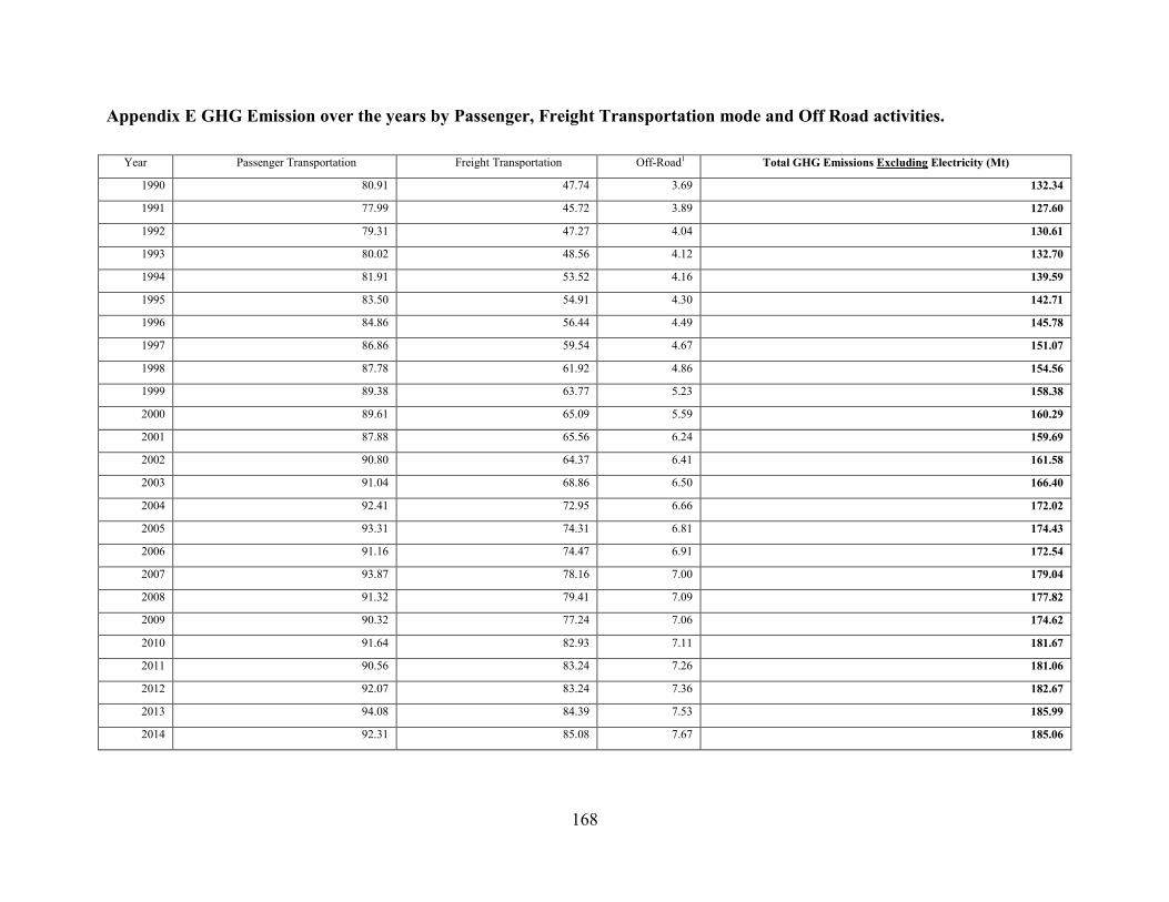
Appendix E GHG Emission over the years by Passenger, Freight Transportation mode and Off
Road activities. ................................................................................................................ 168
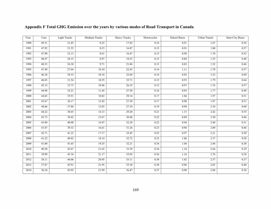
Appendix F Total GHG Emission over the years by various modes of Road Transport in Canada
......................................................................................................................................... 169
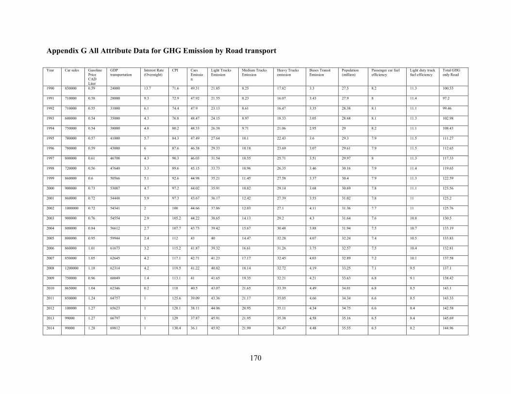
Appendix G All Attribute Data for GHG Emission by Road transport .......................... 170
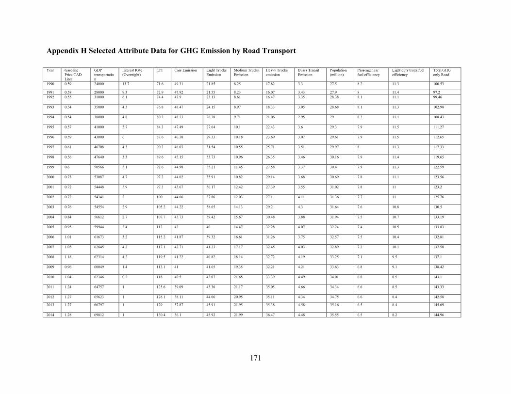
Appendix H Selected Attribute Data for GHG Emission by Road Transport ................ 171
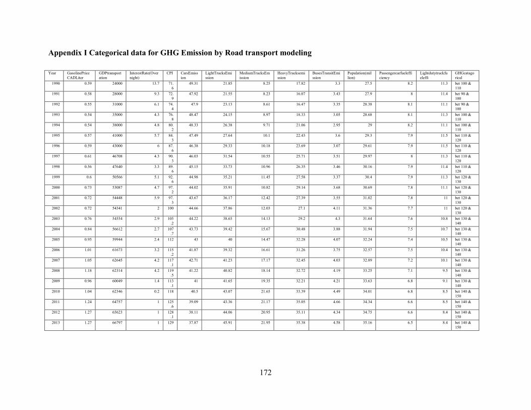
Appendix I Categorical data for GHG Emission by Road transport modeling .............. 172
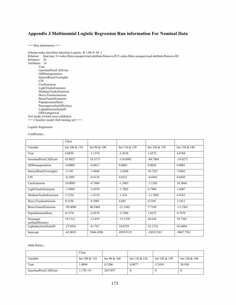
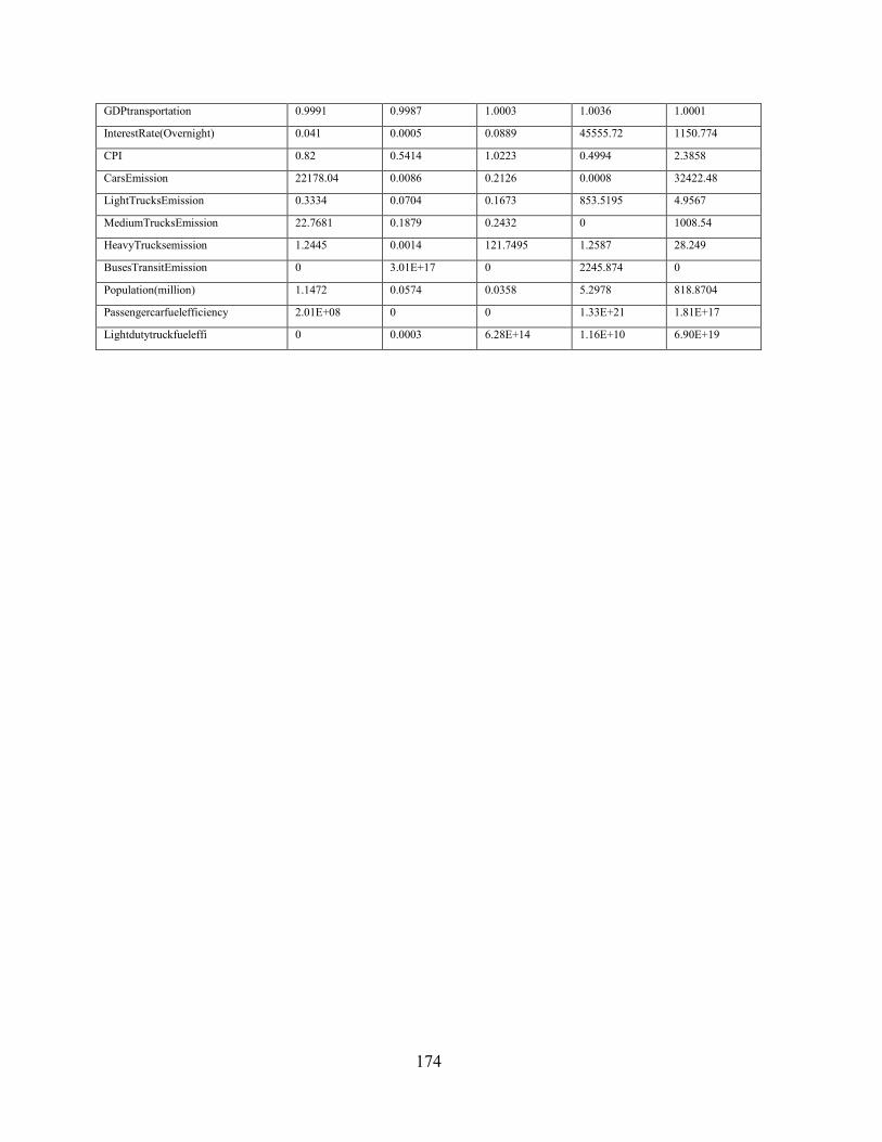
Appendix J Multinomial Logistic Regression Run information For Nominal Data ....... 173
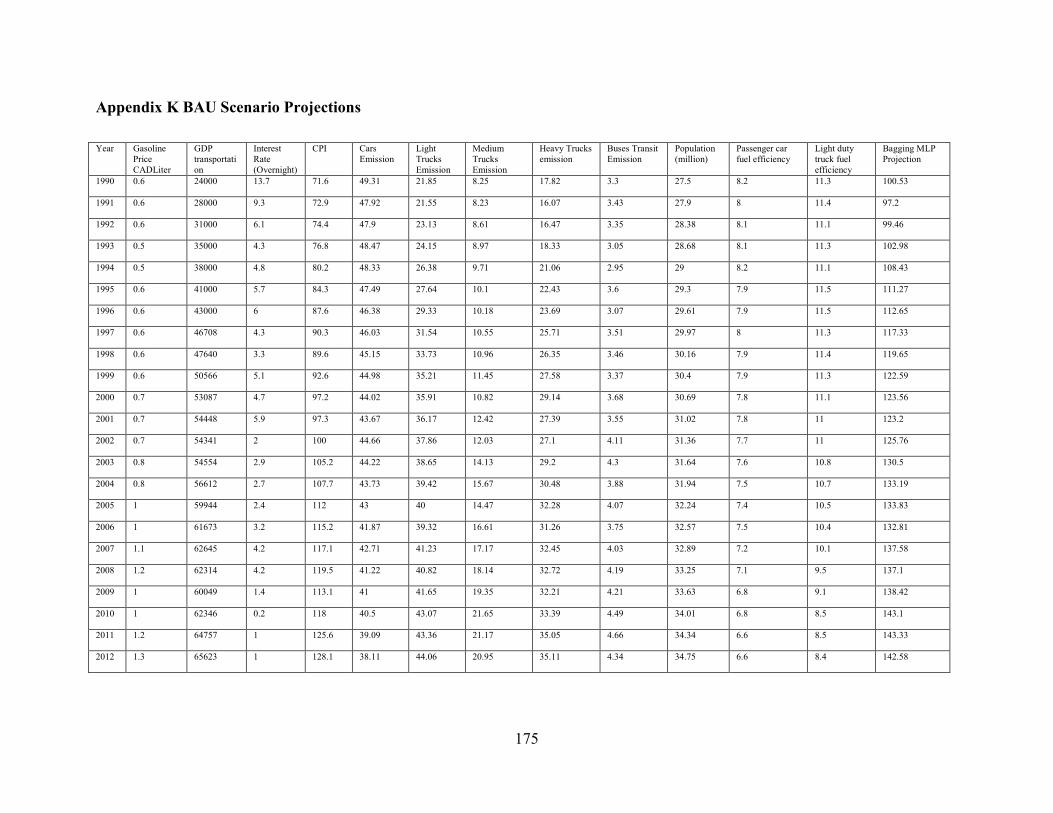
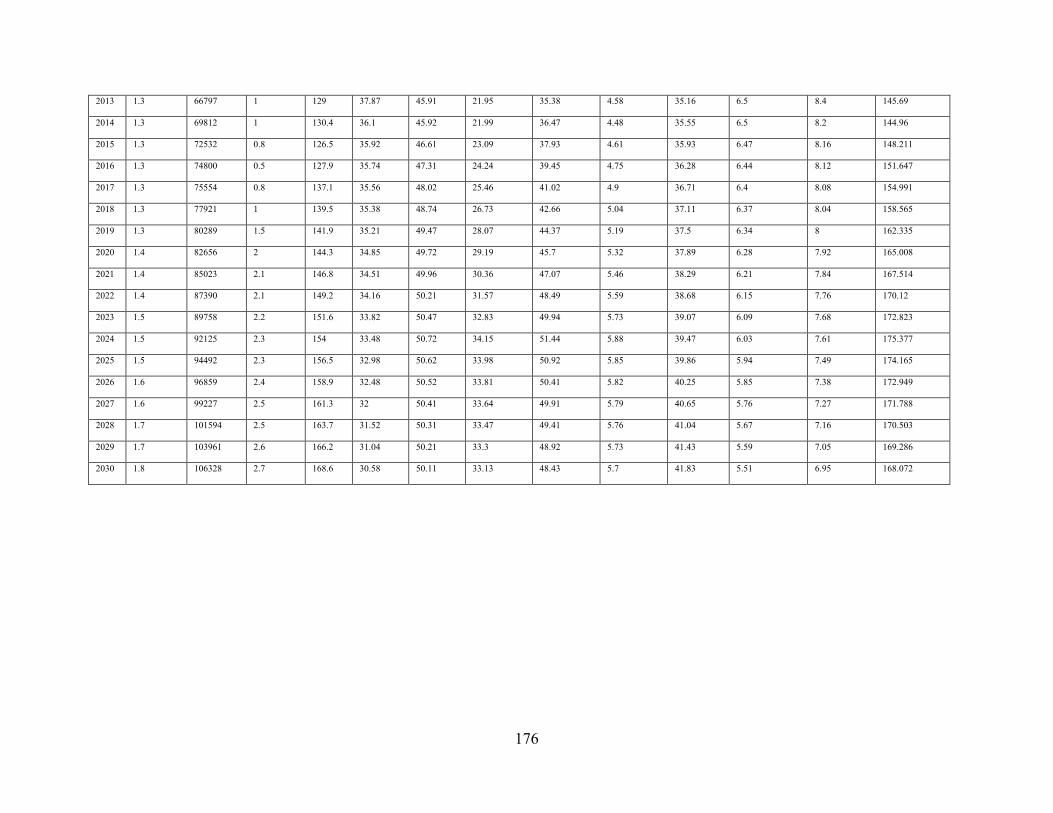
Appendix K BAU Scenario Projections ......................................................................... 175
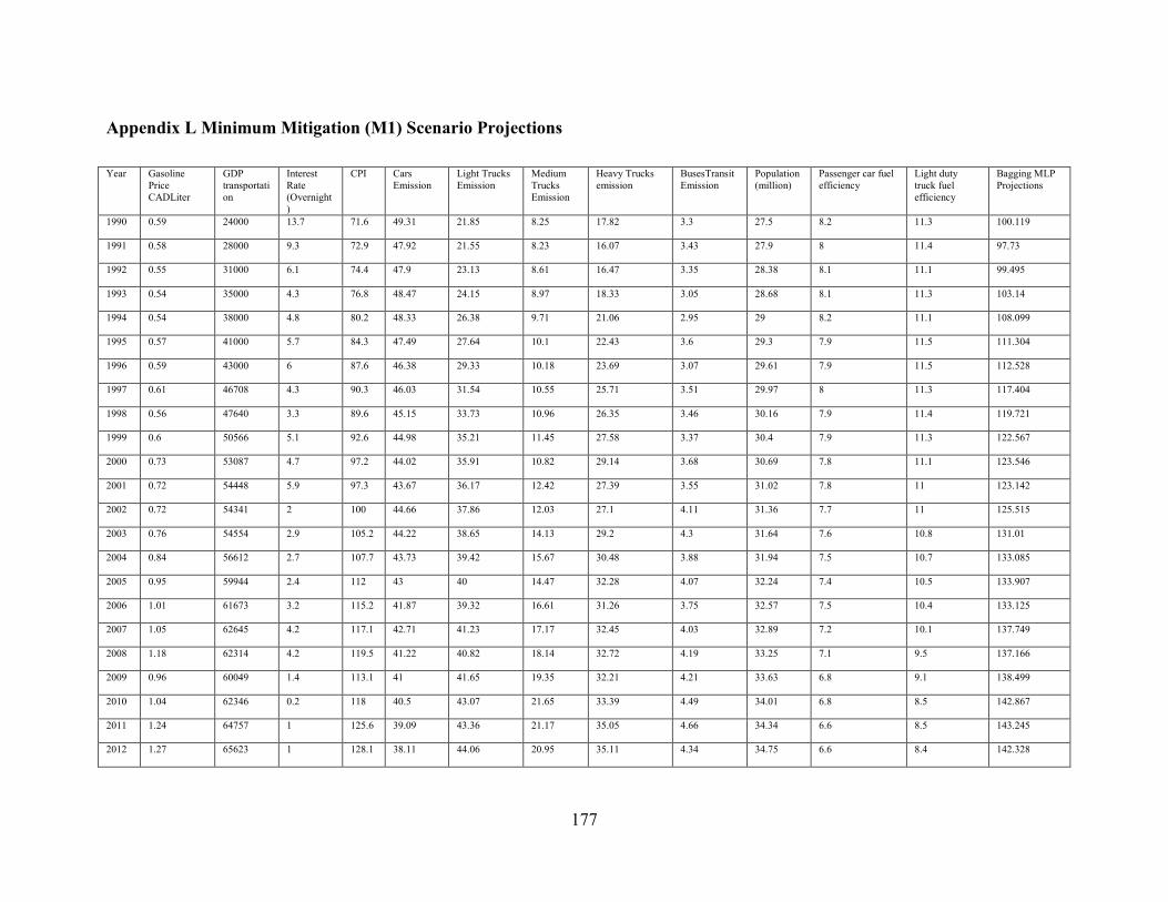
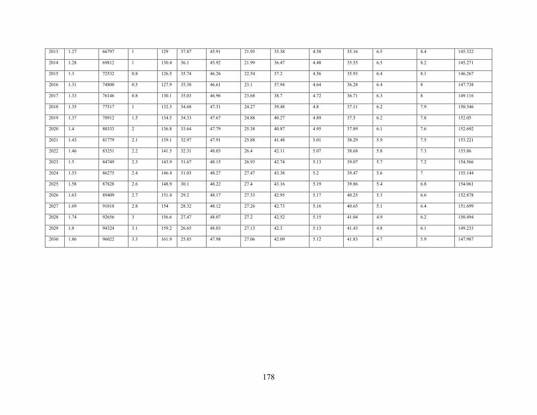
Appendix L Minimum Mitigation (M1) Scenario Projections ....................................... 177
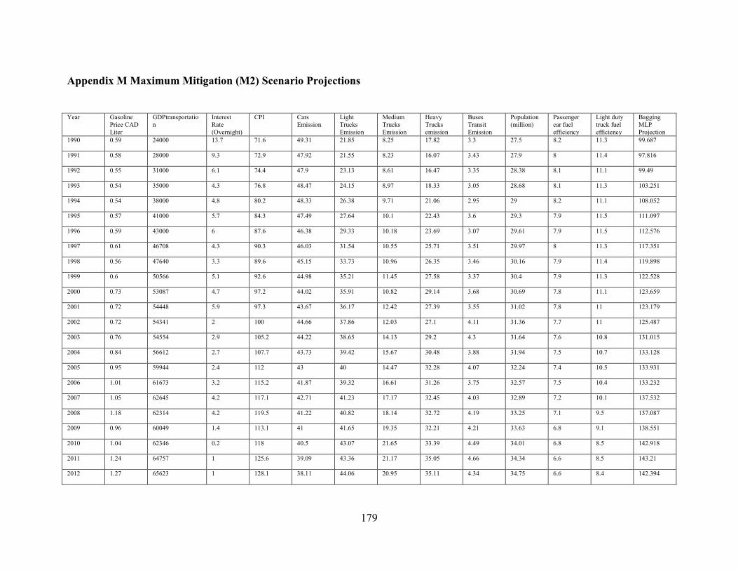
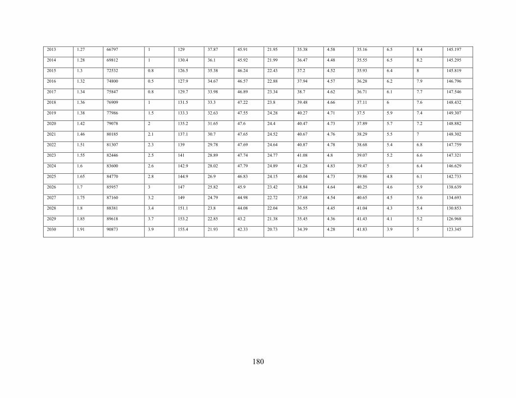
Appendix M Maximum Mitigation (M2) Scenario Projections ..................................... 179
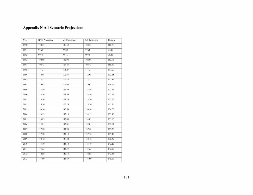
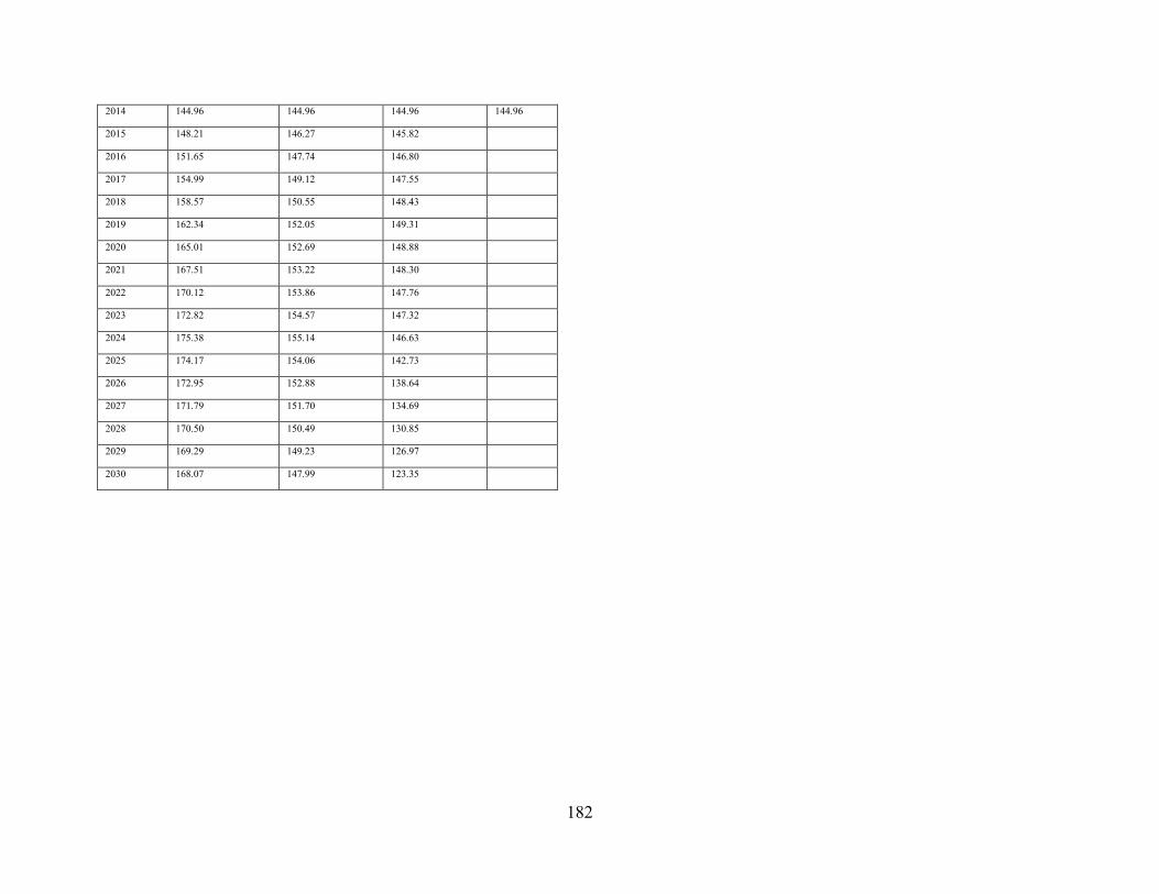
Appendix N All Scenario Projections ............................................................................. 181
Page 11
XI
List of Figures
Figure 1. Required input data for COPERT model (Source: Dimitrios et al., 2012).................... 10
Figure 2 Process of applying supervised machine learning Source: (Kotsiantis et al., 2007). ..... 24 Figure 3 Artificial model of a Neuron. Source: (de Pina et al., 2016). ......................................... 32 Figure 4 Output Sigmoid Activation Function. Source: (de Pina et al., 2016) ............................. 33 Figure 5 Multilayer Perceptron with Three Layers. Source: (Mirjalili et al., 2014). .................... 34 Figure 6 Error Surface as Function of a Weight Showing Gradient and Local and Global Minima.
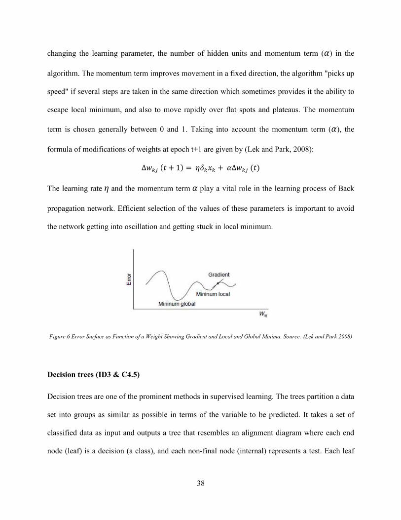
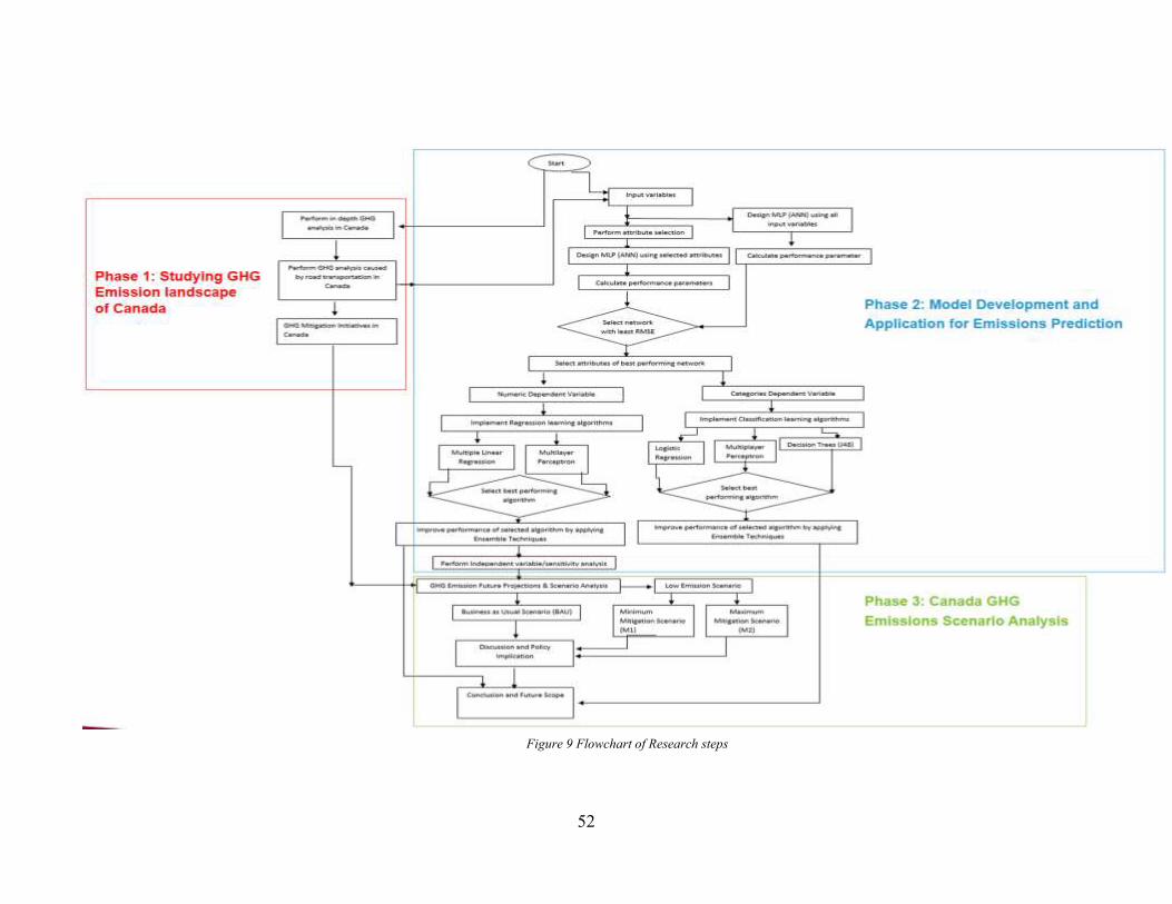
Source: (Lek and Park 2008) ........................................................................................................ 38 Figure 7. General Ensemble Architecture. Source: (Zhou 2012). ................................................ 43 Figure 8. Classifier Performance Marked on Noise Level vs. Error. Source: (Zhou 2012). ........ 44 Figure 9 Flowchart of Research steps ........................................................................................... 52
Figure 10 Total GHG Emissions over the Years (MtCo2eq.) ...................................................... 54 Figure 11. GHG Emission by Canadian Economic Sector ........................................................... 56
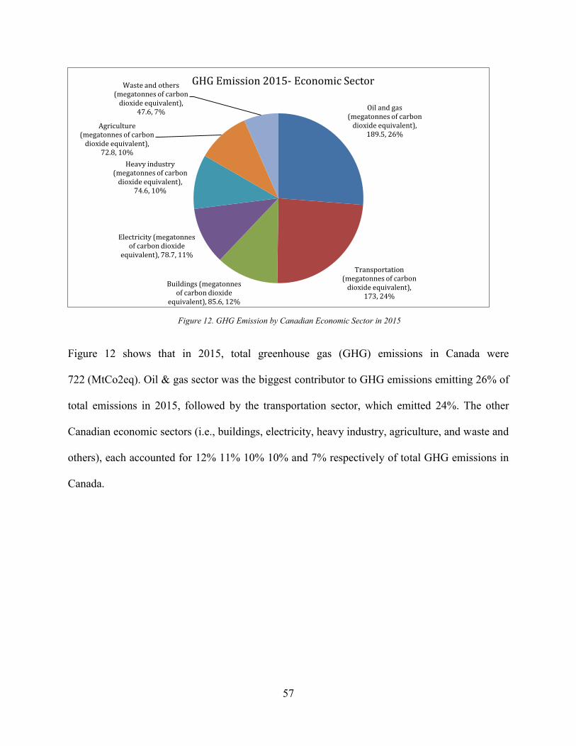
Figure 12. GHG Emission by Canadian Economic Sector in 2015 .............................................. 57 Figure 13. Provincial GHG Emissions over the Years ................................................................. 59
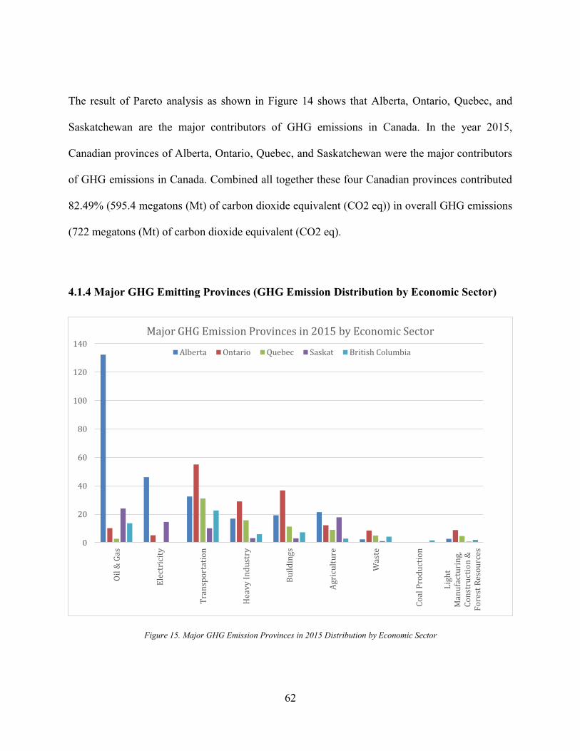
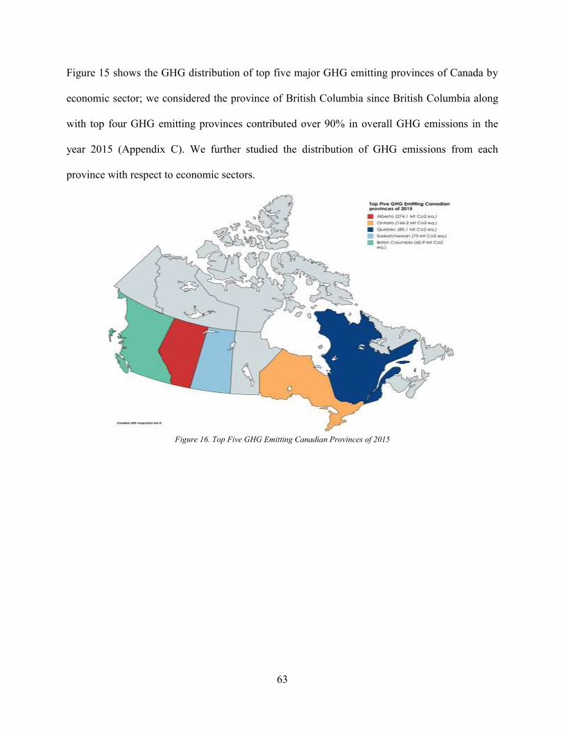
Figure 14. Pareto Analysis of GHG Emissions by Provinces in 2015.......................................... 61 Figure 15. Major GHG Emission Provinces in 2015 Distribution by Economic Sector .............. 62 Figure 16. Top Five GHG Emitting Canadian Provinces of 2015 ................................................ 63
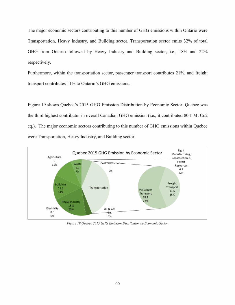
Figure 17. Alberta 2015 GHG Emission Distribution by Economic Sector ................................. 64 Figure 18. Ontario 2015 GHG Emission Distribution by Economic Sector................................. 64 Figure 19 Quebec 2015 GHG Emission Distribution by Economic Sector.................................. 65
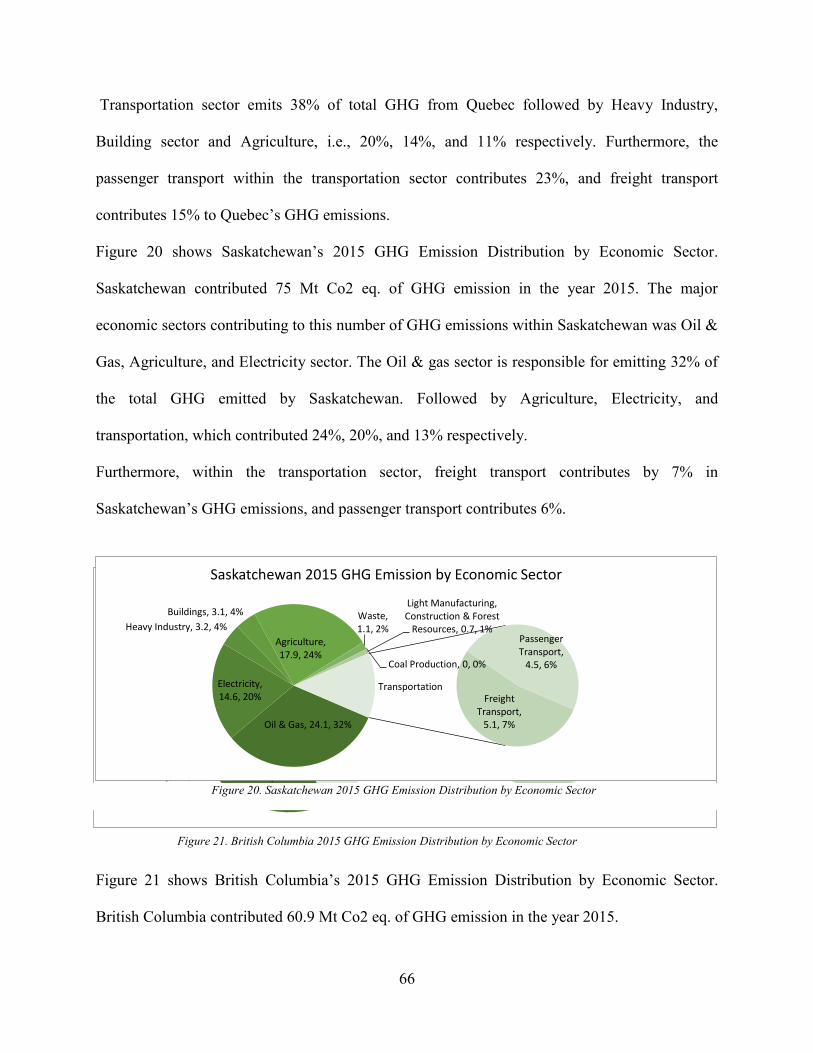
Figure 20. Saskatchewan 2015 GHG Emission Distribution by Economic Sector ...................... 66 Figure 21. British Columbia 2015 GHG Emission Distribution by Economic Sector ................. 66
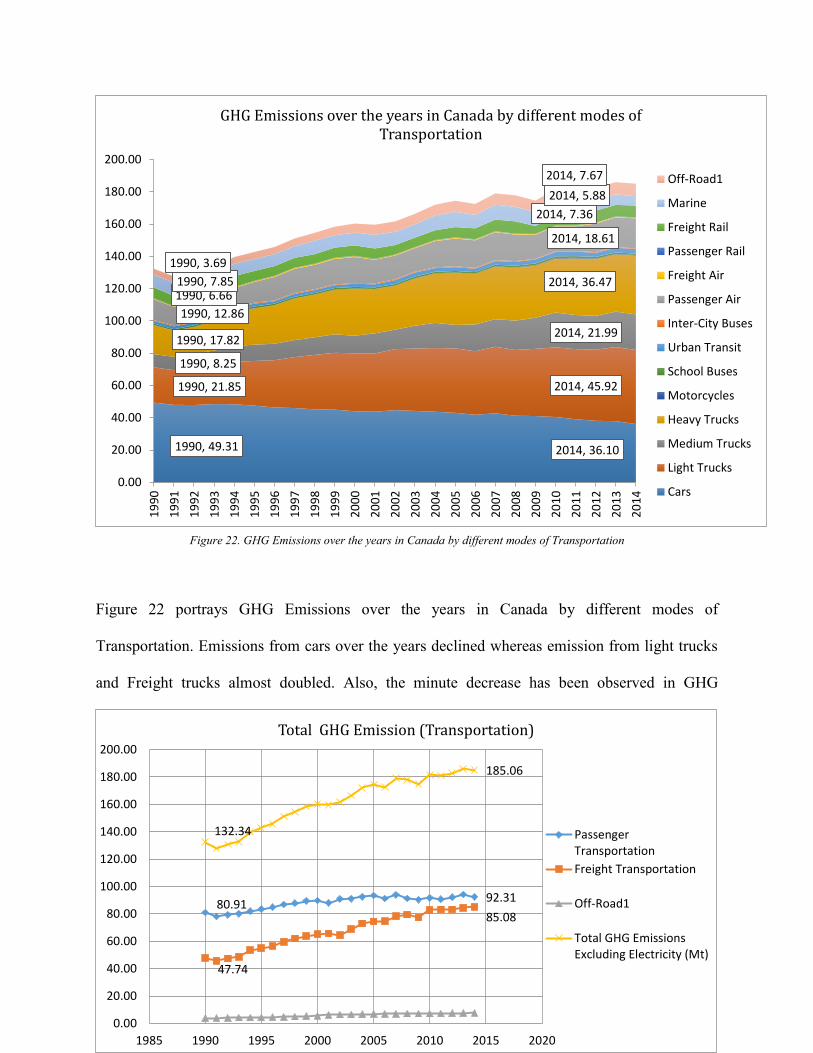
Figure 22. GHG Emissions over the years in Canada by different modes of Transportation ...... 68
Figure 23. Total GHG Emission by Transportation Sector .......................................................... 69
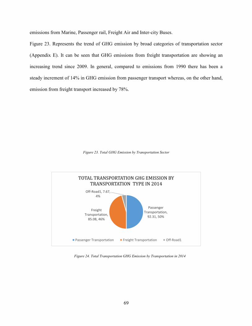
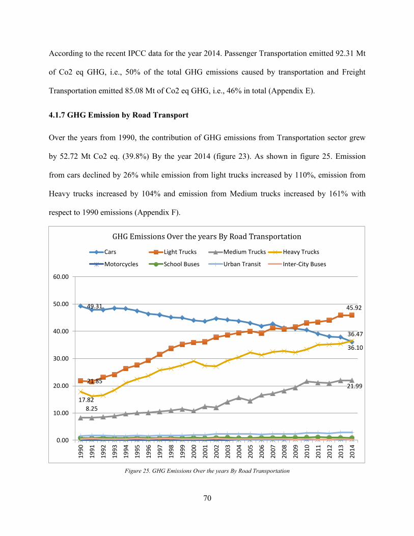
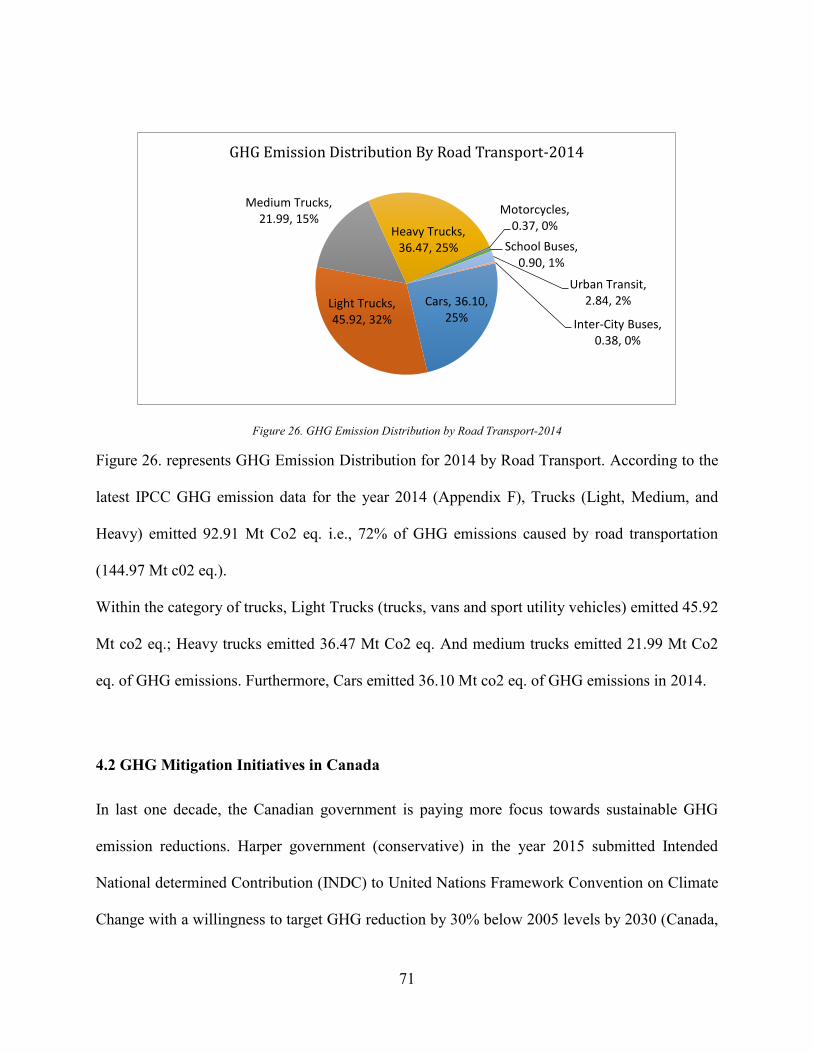
Figure 24. Total Transportation GHG Emission by Transportation in 2014 ................................ 69 Figure 25. GHG Emissions Over the years By Road Transportation ........................................... 70
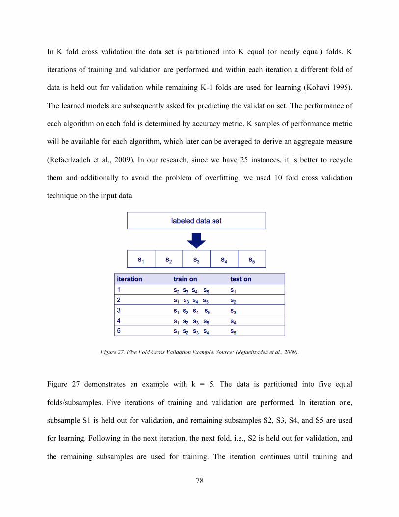
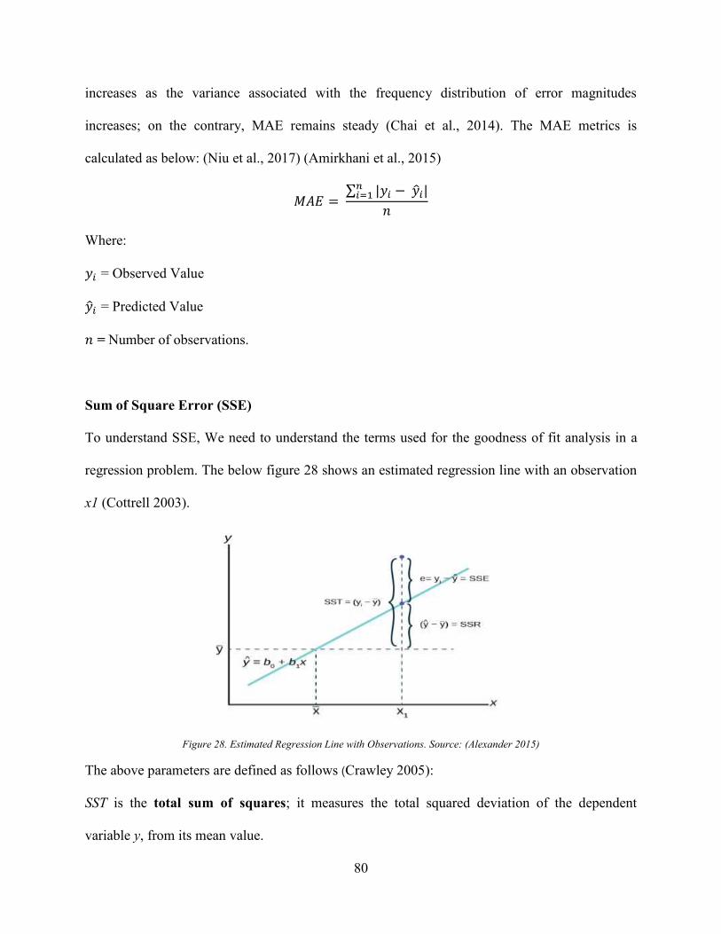
Figure 26. GHG Emission Distribution by Road Transport-2014 ................................................ 71 Figure 27. Five Fold Cross Validation Example. Source: (Refaeilzadeh et al., 2009). ................ 78 Figure 28. Estimated Regression Line with Observations. Source: (Alexander 2015) ................ 80
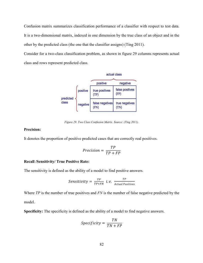
Figure 29. Two Class Confusion Matrix. Source: (Ting 2011). ................................................... 82 Figure 30. ROC Curve Example. Source: (Fawcett 2006). .......................................................... 85
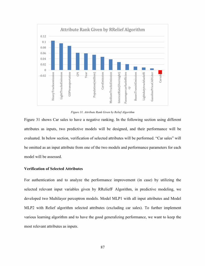
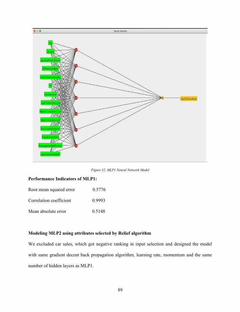
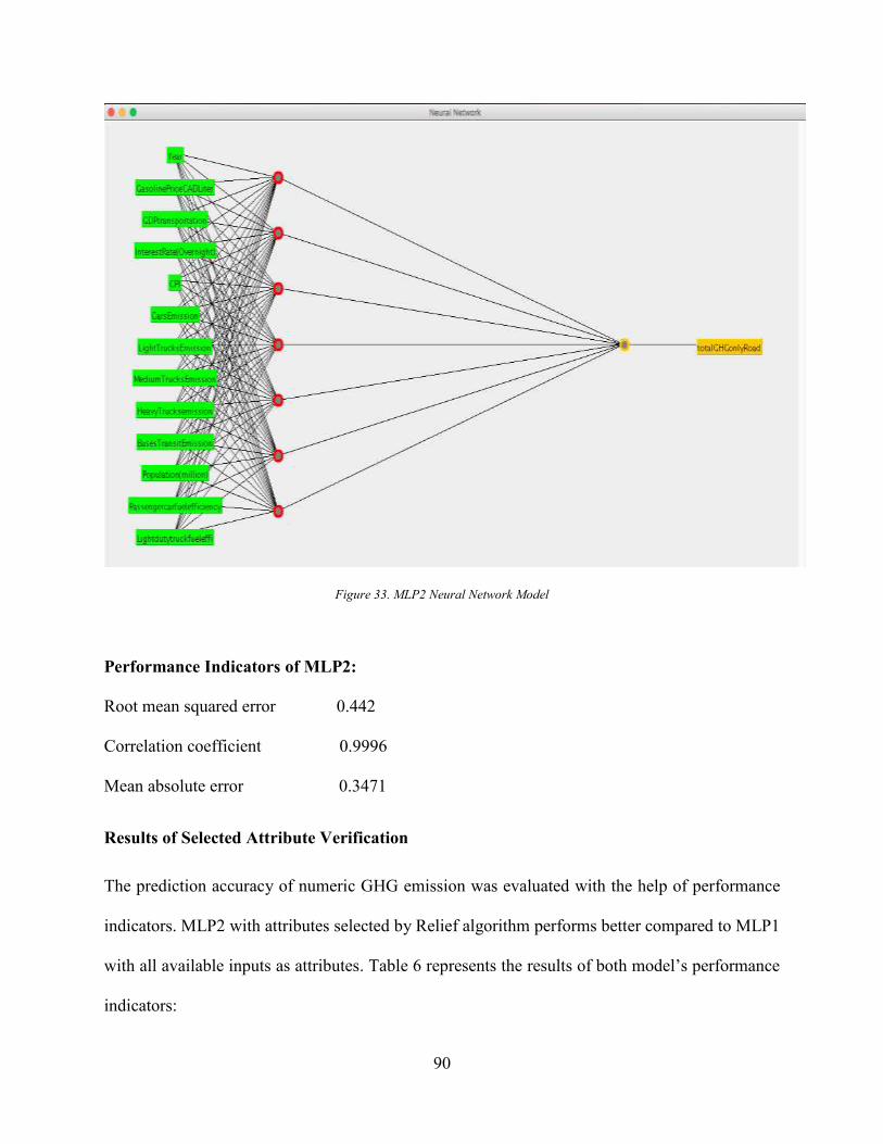
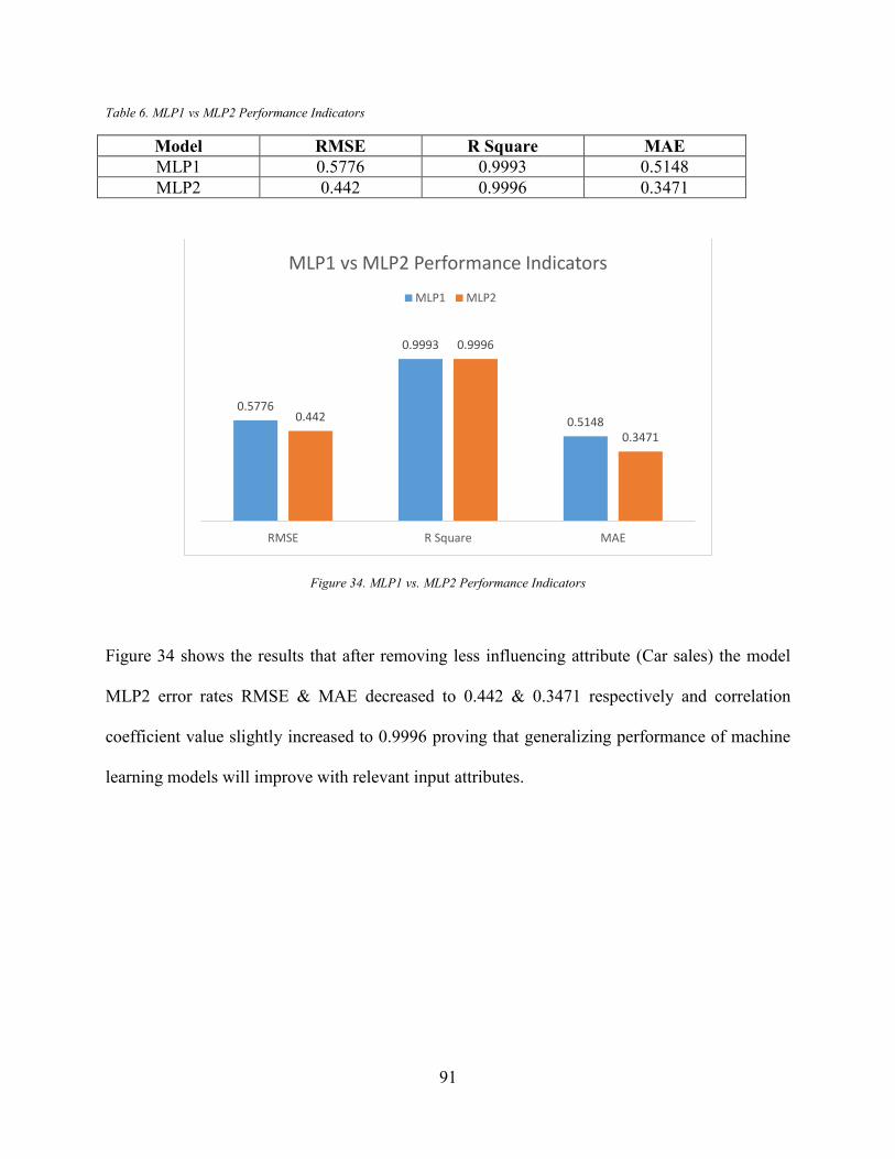
Figure 31. Attribute Rank Given by Relief Algorithm ................................................................. 87 Figure 32. MLP1 Neural Network Model..................................................................................... 89 Figure 33. MLP2 Neural Network Model..................................................................................... 90 Figure 34. MLP1 vs. MLP2 Performance Indicators .................................................................... 91
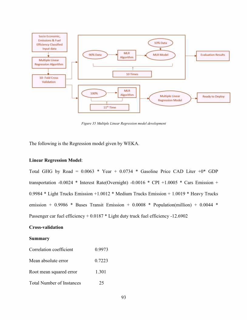
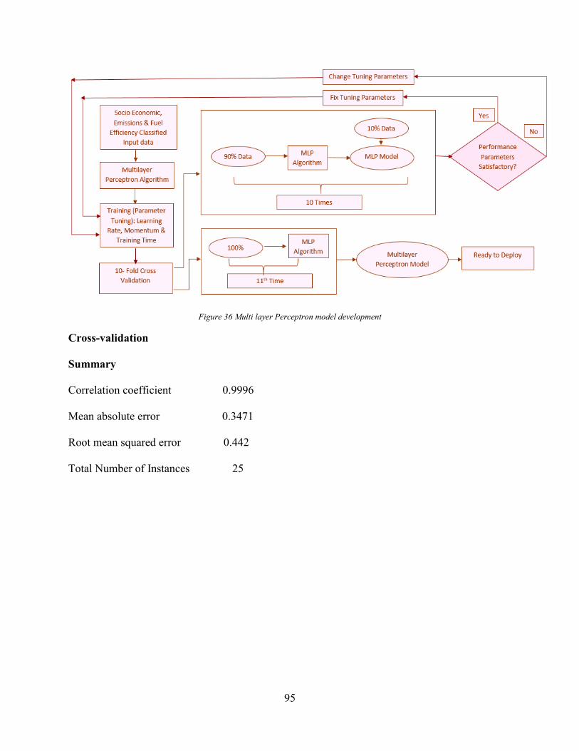
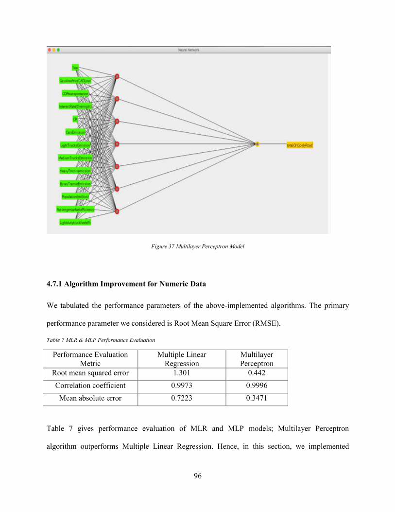
Figure 35 Multiple Linear Regression model development ......................................................... 93 Figure 36 Multi layer Perceptron model development ................................................................. 95 Figure 37 Multilayer Perceptron Model ....................................................................................... 96
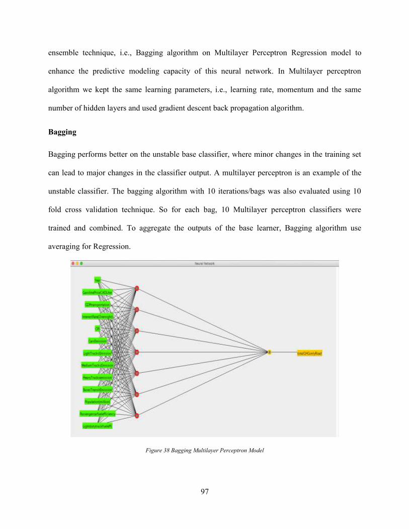
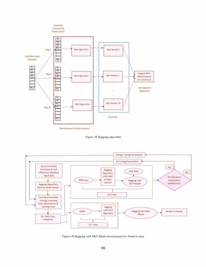
Figure 38 Bagging Multilayer Perceptron Model ......................................................................... 97 Figure 39 Bagging algorithm ........................................................................................................ 98 Figure 40 Bagging with MLP Model development for Numeric data .......................................... 98 Figure 41 Performance Indicators of Algorithms on Numeric Data ........................................... 100 Figure 42 Multinomial Logistic regression model development ................................................ 102
Page 12
XII
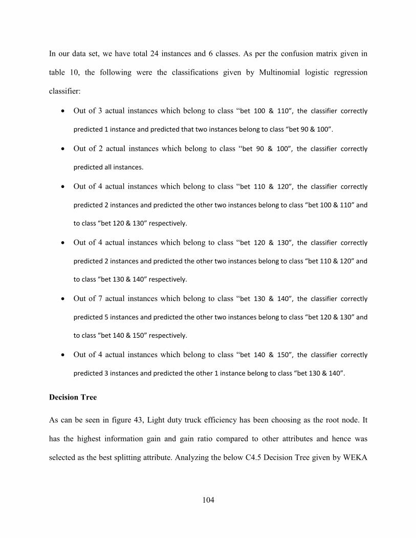
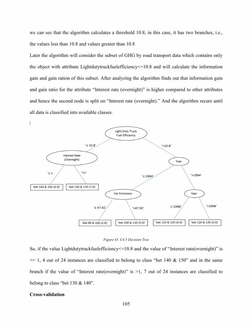
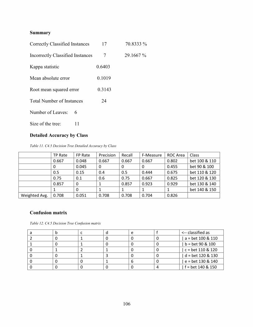
Figure 43. C4.5 Decision Tree .................................................................................................... 105
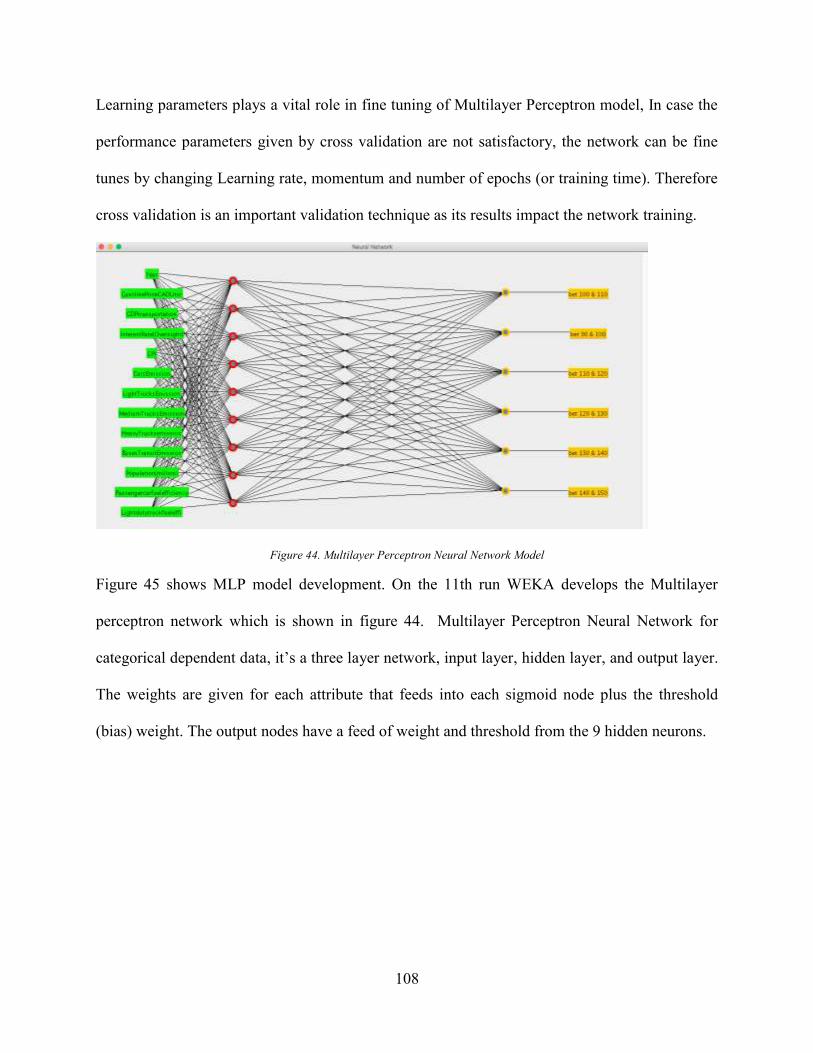
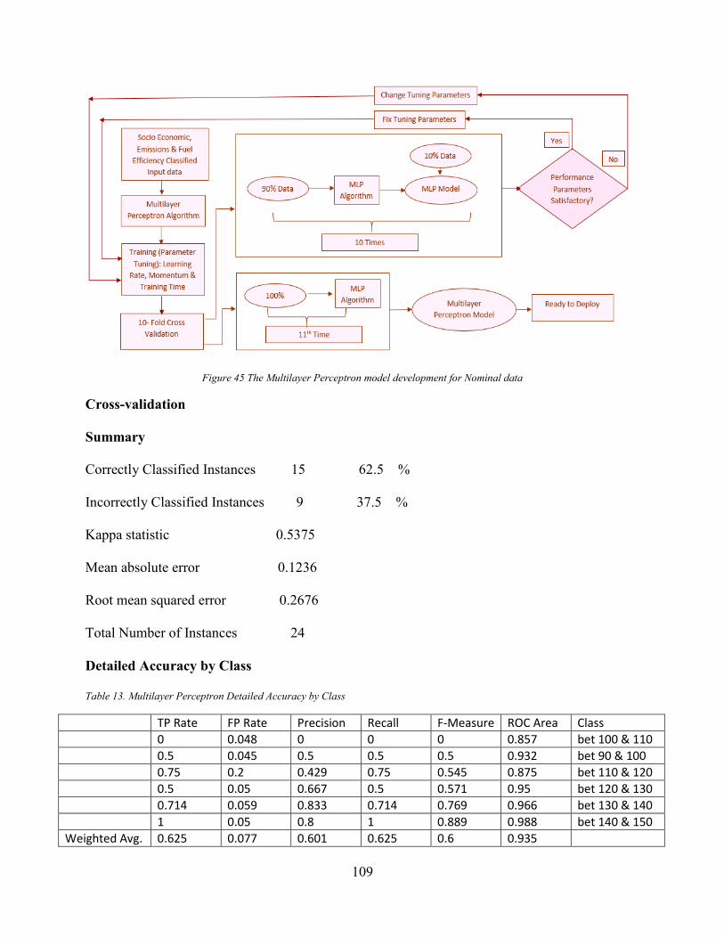
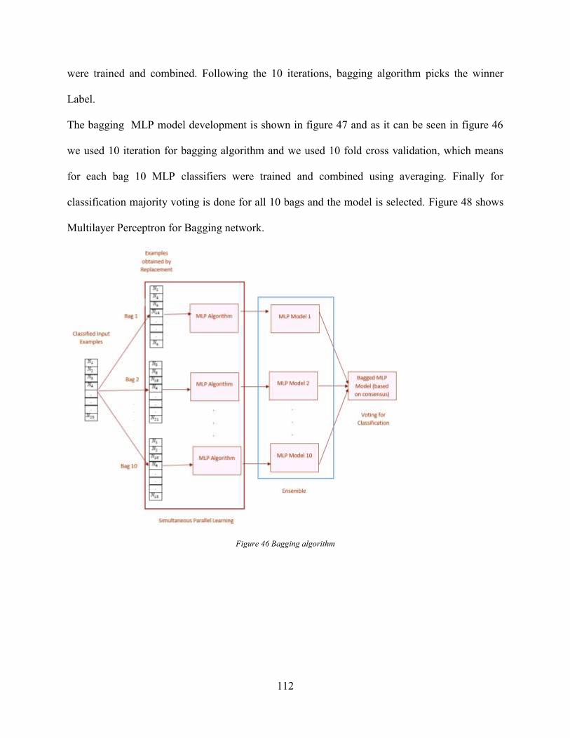
Figure 44. Multilayer Perceptron Neural Network Model.......................................................... 108 Figure 45 The Multilayer Perceptron model development for Nominal data ............................. 109 Figure 46 Bagging algorithm ...................................................................................................... 112
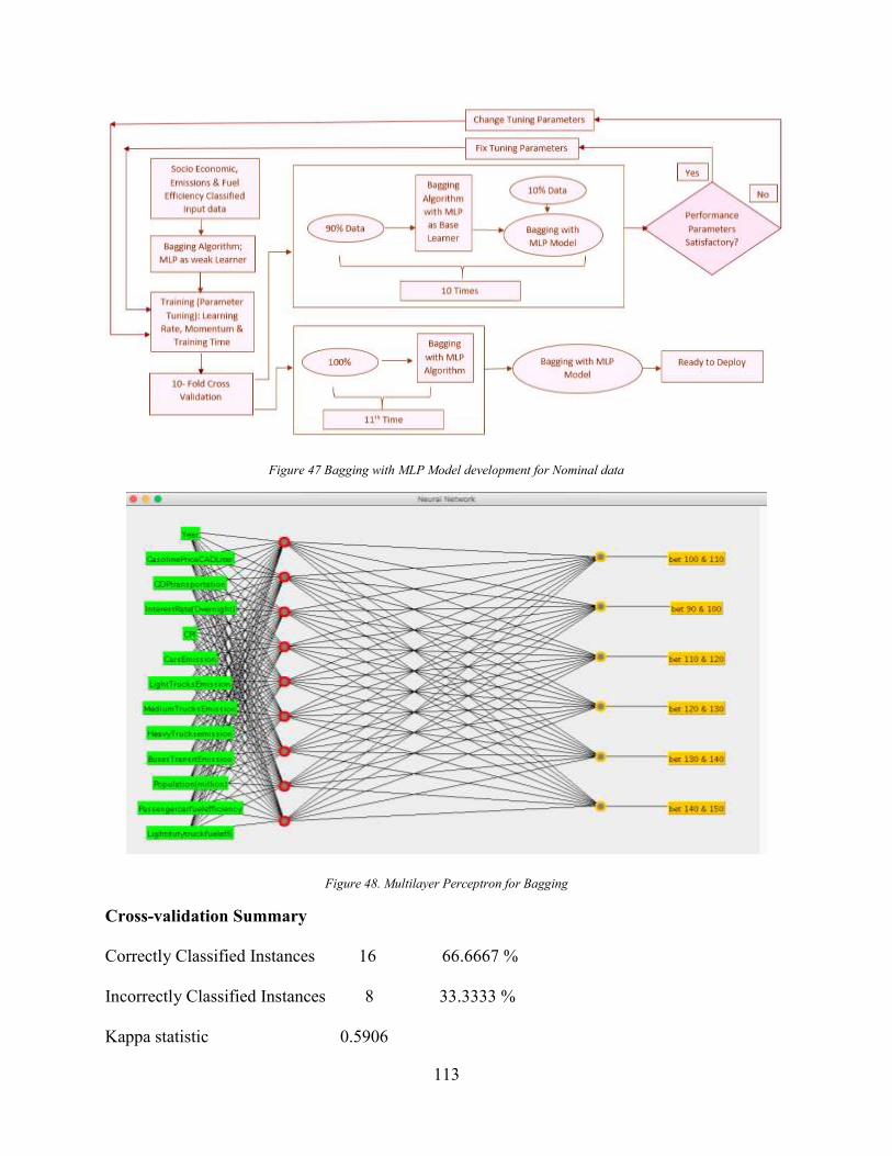
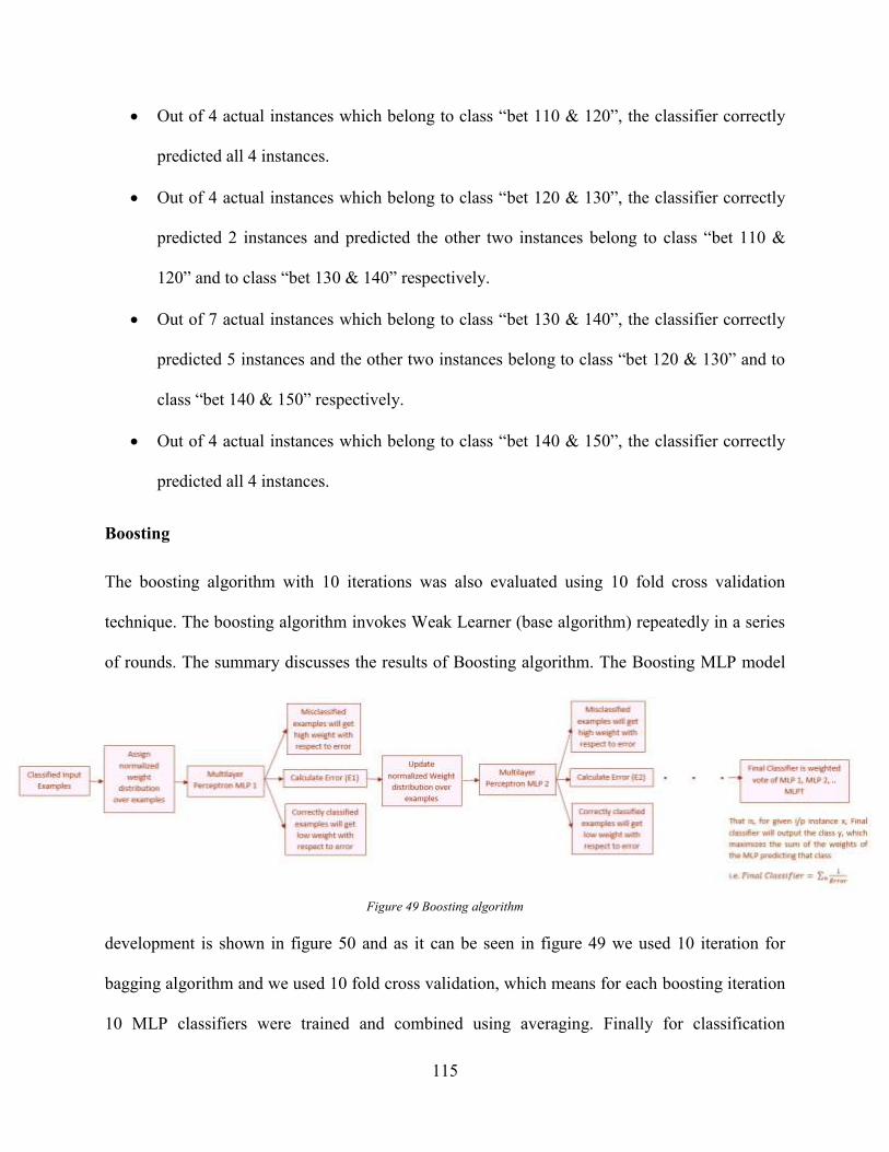
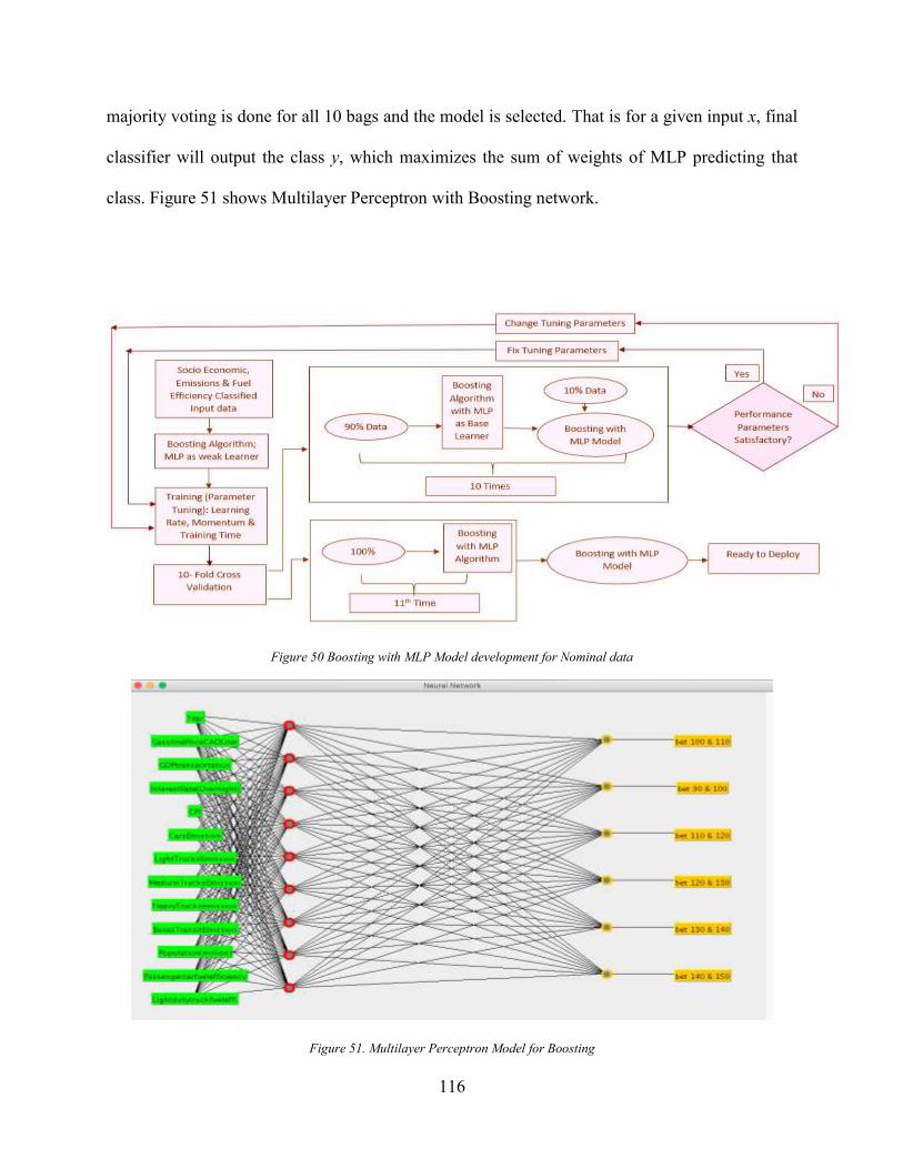
Figure 47 Bagging with MLP Model development for Nominal data ........................................ 113 Figure 48. Multilayer Perceptron for Bagging ............................................................................ 113 Figure 49 Boosting algorithm ..................................................................................................... 115 Figure 50 Boosting with MLP Model development for Nominal data ....................................... 116 Figure 51. Multilayer Perceptron Model for Boosting ............................................................... 116
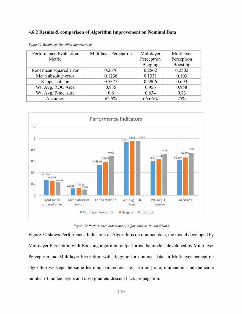
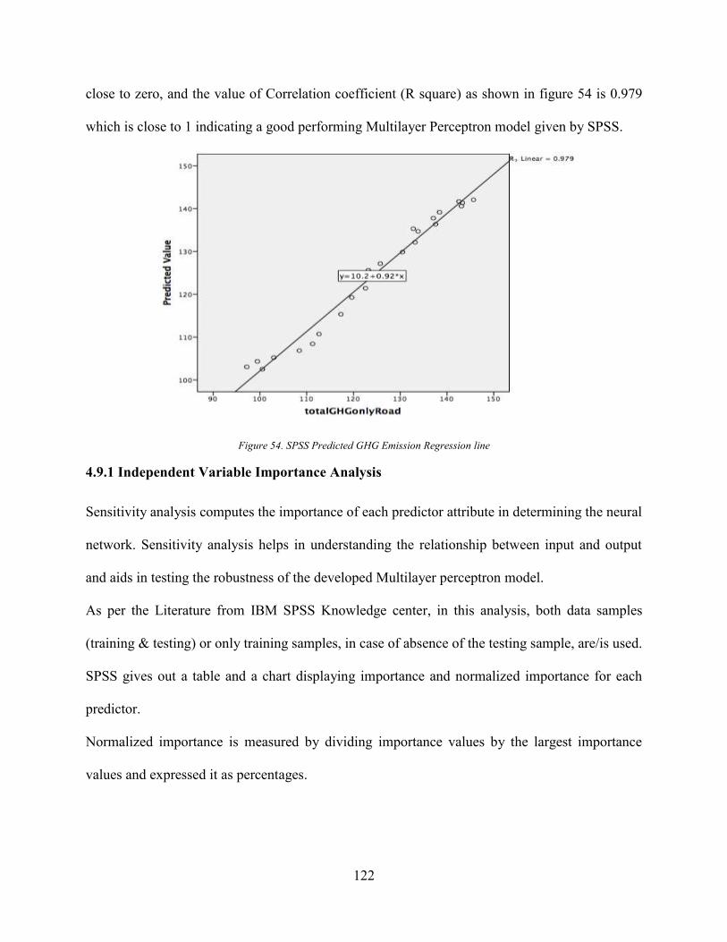
Figure 52 Performance Indicators of Algorithms on Nominal Data ........................................... 119 Figure 53. MLP Model for Numeric GHG Emission Values developed in SPSS ...................... 120 Figure 54. SPSS Predicted GHG Emission Regression line ....................................................... 122 Figure 55MLP Attribute Normalized Importance ...................................................................... 123
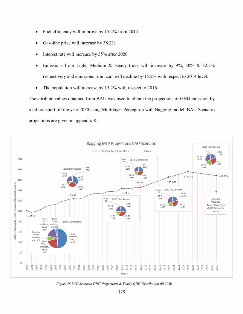
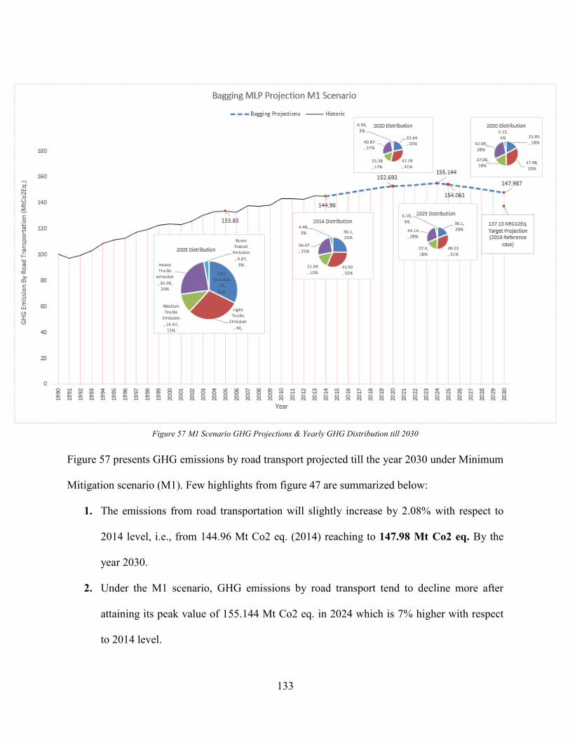
Figure 56 BAU Scenario GHG Projections & Yearly GHG Distribution till 2030.................... 129 Figure 57 M1 Scenario GHG Projections & Yearly GHG Distribution till 2030 ...................... 133
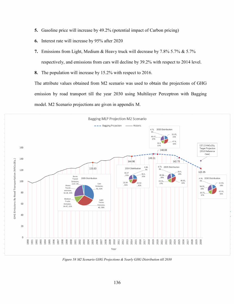
Figure 58 M2 Scenario GHG Projections & Yearly GHG Distribution till 2030 ...................... 136 Figure 59 All Scenario Projections till 2030............................................................................... 138
Figure 60 SWOT Analysis .......................................................................................................... 144
Page 13
XIII
List of Tables Table 1 Methods in the Field of GHG Emission Modeling and Estimation ................................. 15
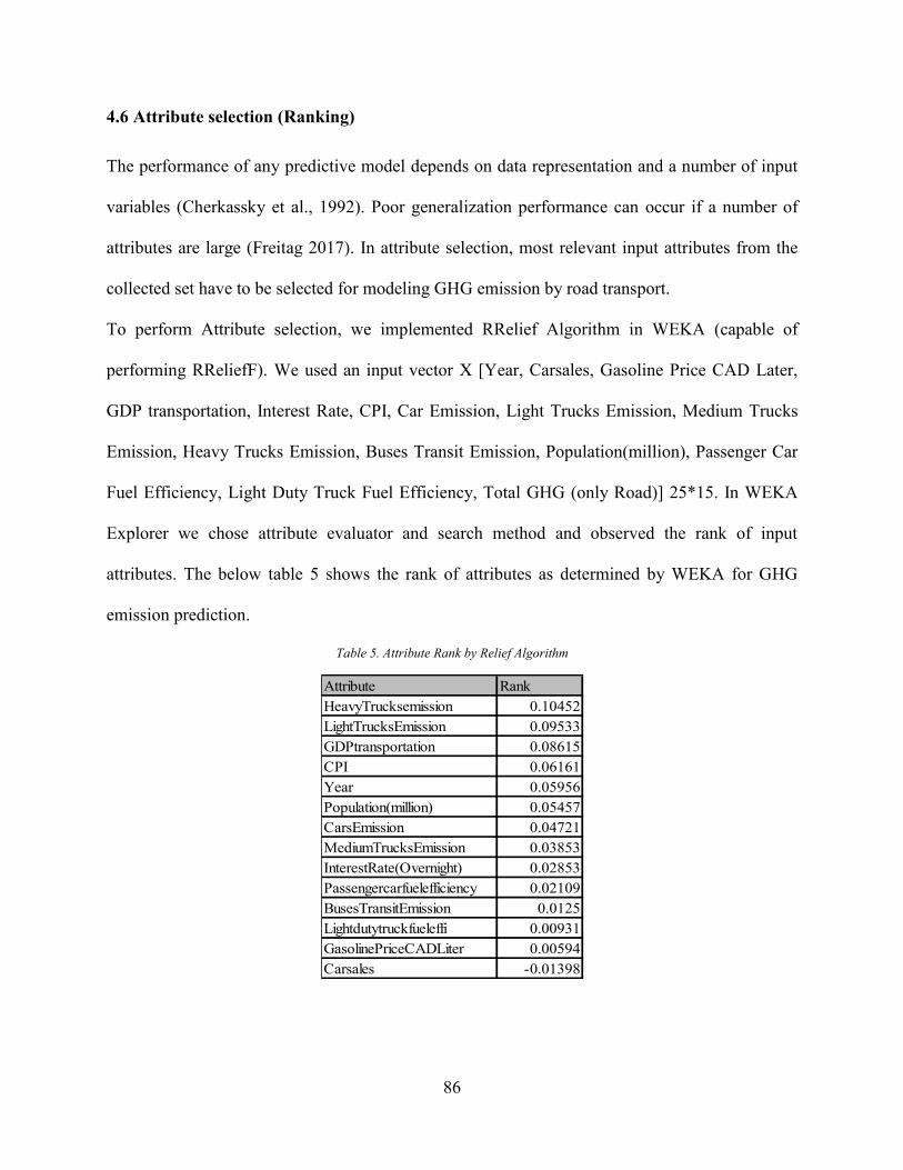
Table 2. Domains Benefitted By Ensemble Techniques .............................................................. 45 Table 3. Bagging Pseudo Code. Source: (King et al., 2014) ........................................................ 46 Table 4 Canada provincial commitments, policy measures and plans ......................................... 72 Table 5. Attribute Rank by Relief Algorithm ............................................................................... 86 Table 6. MLP1 vs MLP2 Performance Indicators ........................................................................ 91
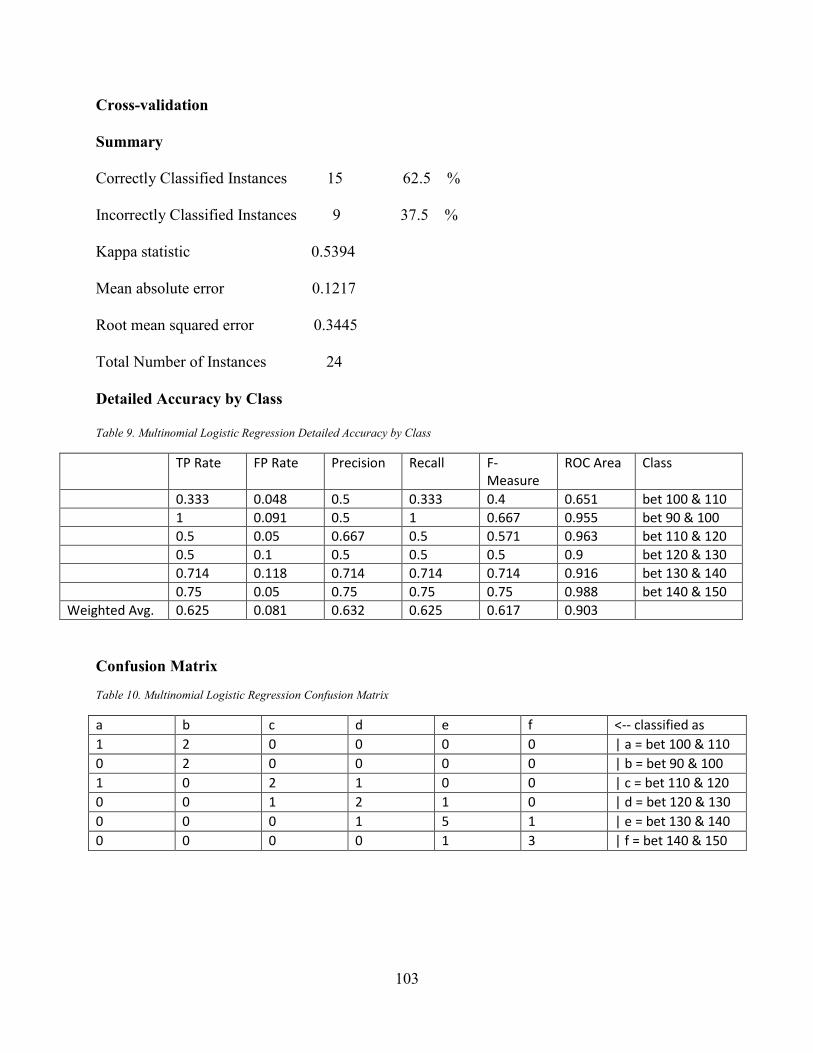
Table 7 MLR & MLP Performance Evaluation ............................................................................ 96 Table 8 Results of Algorithm Improvement on Numeric Data..................................................... 99 Table 9. Multinomial Logistic Regression Detailed Accuracy by Class .................................... 103 Table 10. Multinomial Logistic Regression Confusion Matrix .................................................. 103 Table 11. C4.5 Decision Tree Detailed Accuracy by Class ........................................................ 106
Table 12. C4.5 Decision Tree Confusion matrix ........................................................................ 106 Table 13. Multilayer Perceptron Detailed Accuracy by Class .................................................... 109
Table 14. Multilayer Perceptron Confusion matrix .................................................................... 110
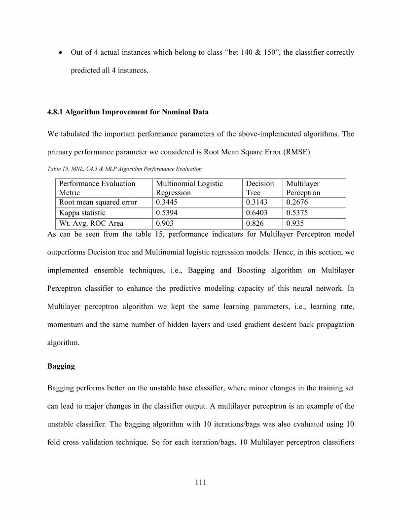
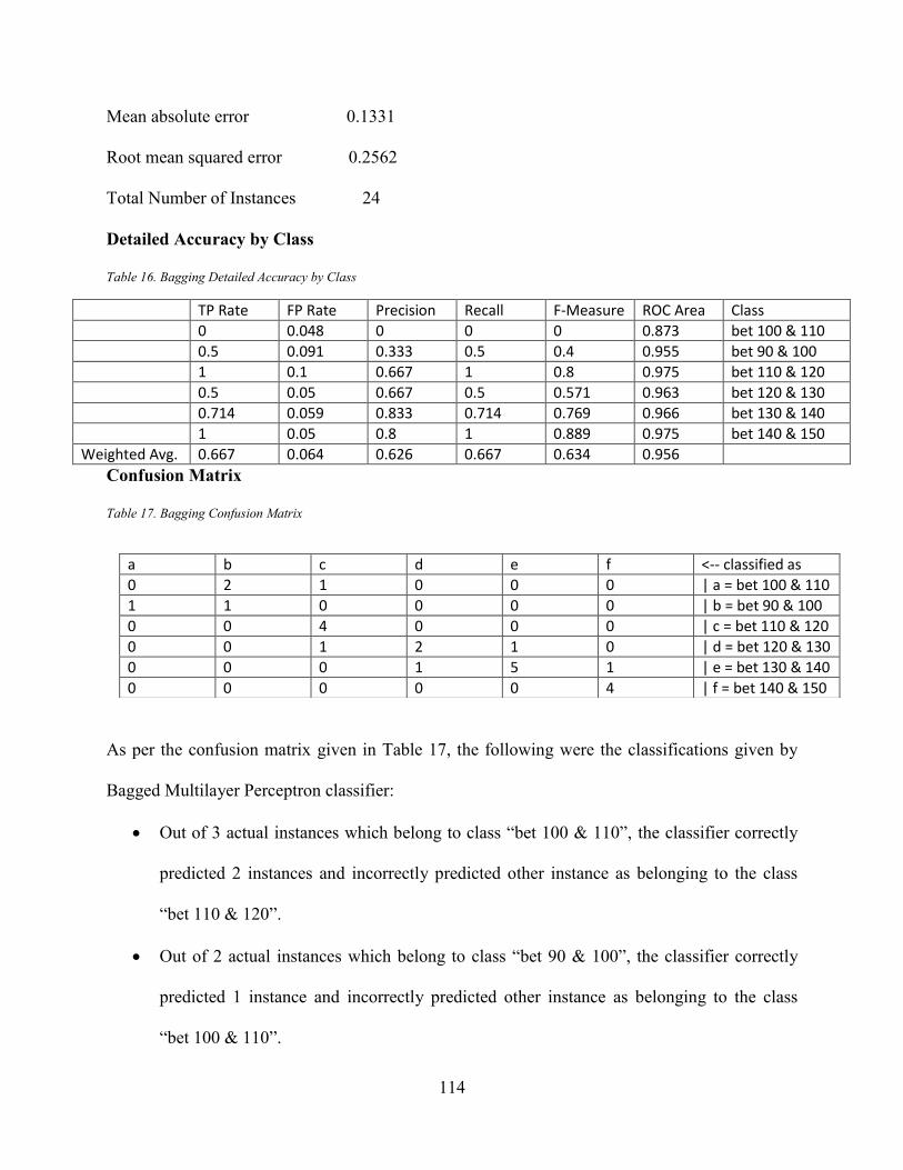
Table 15. MNL, C4.5 & MLP Algorithm Performance Evaluation ........................................... 111 Table 16. Bagging Detailed Accuracy by Class ......................................................................... 114 Table 17. Bagging Confusion Matrix ......................................................................................... 114
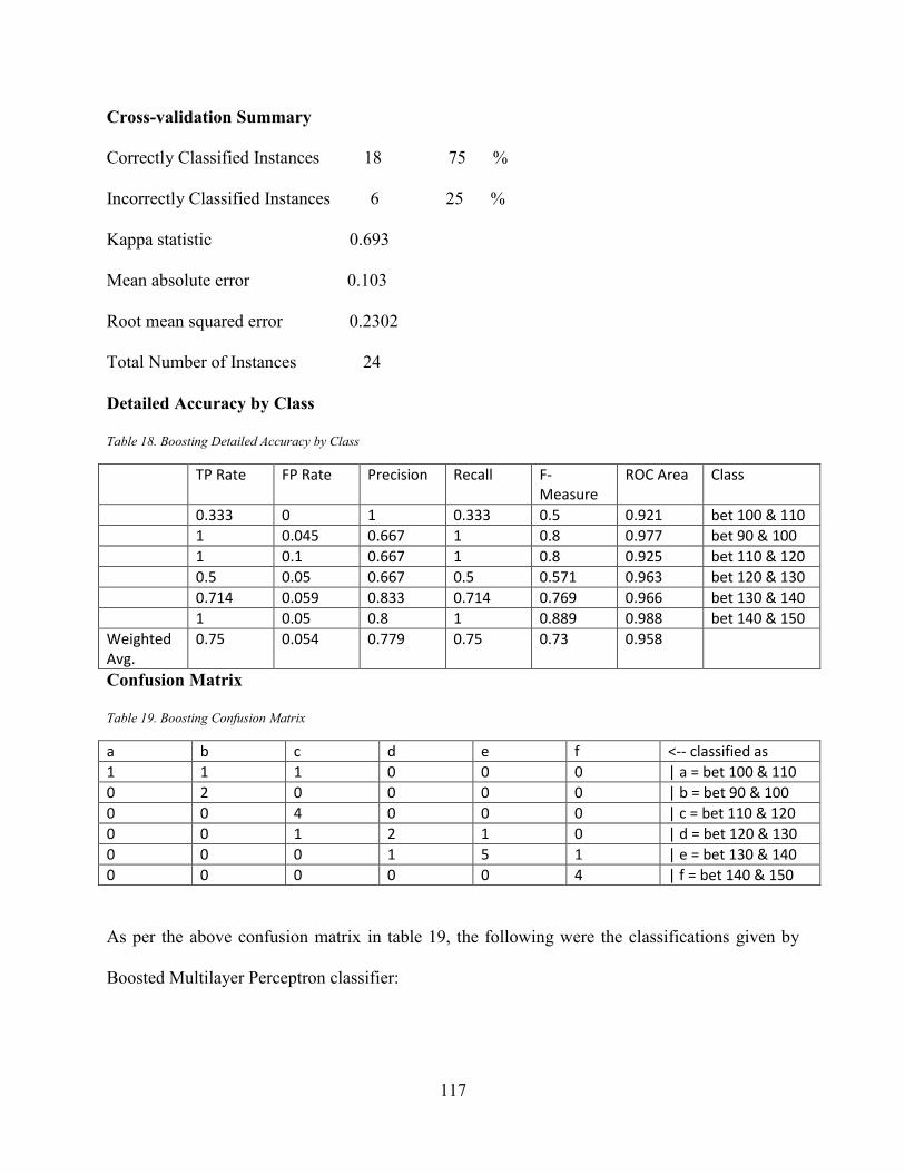
Table 18. Boosting Detailed Accuracy by Class ........................................................................ 117 Table 19. Boosting Confusion Matrix ........................................................................................ 117
Table 20. Results of Algorithm Improvement ............................................................................ 119 Table 21.SPSS Network Information ........................................................................................ 121 Table 22. Summary of Model Developed in SPSS ..................................................................... 121
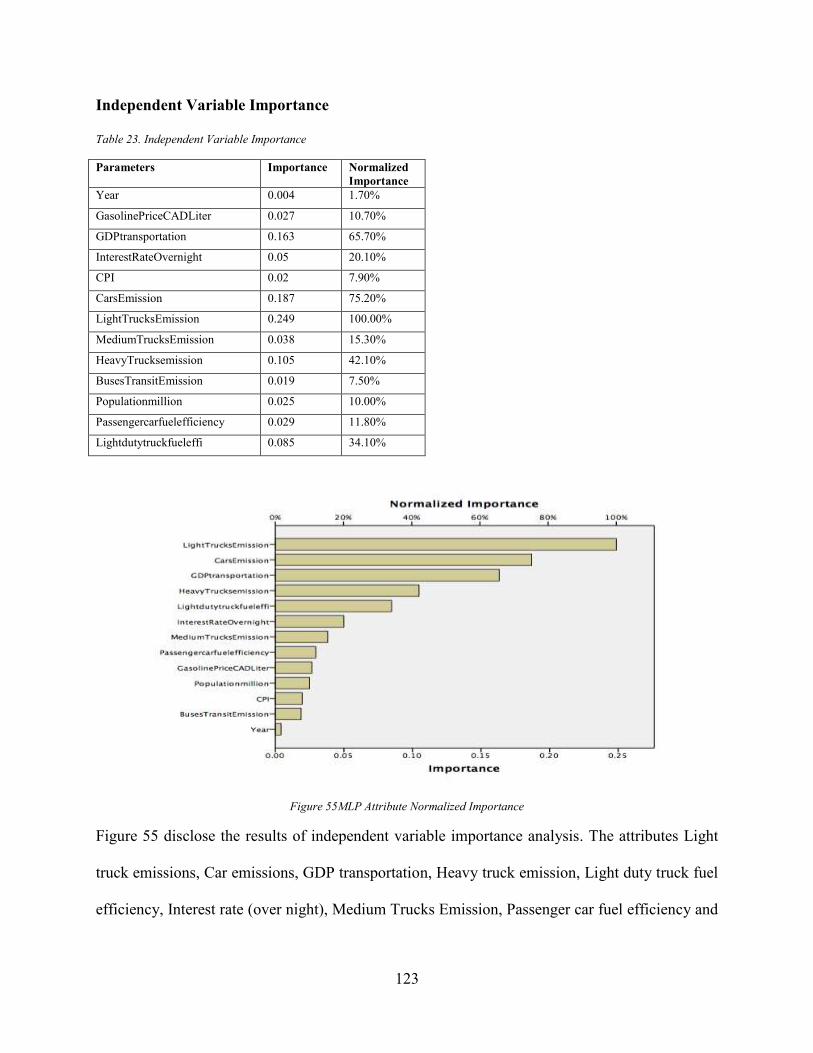
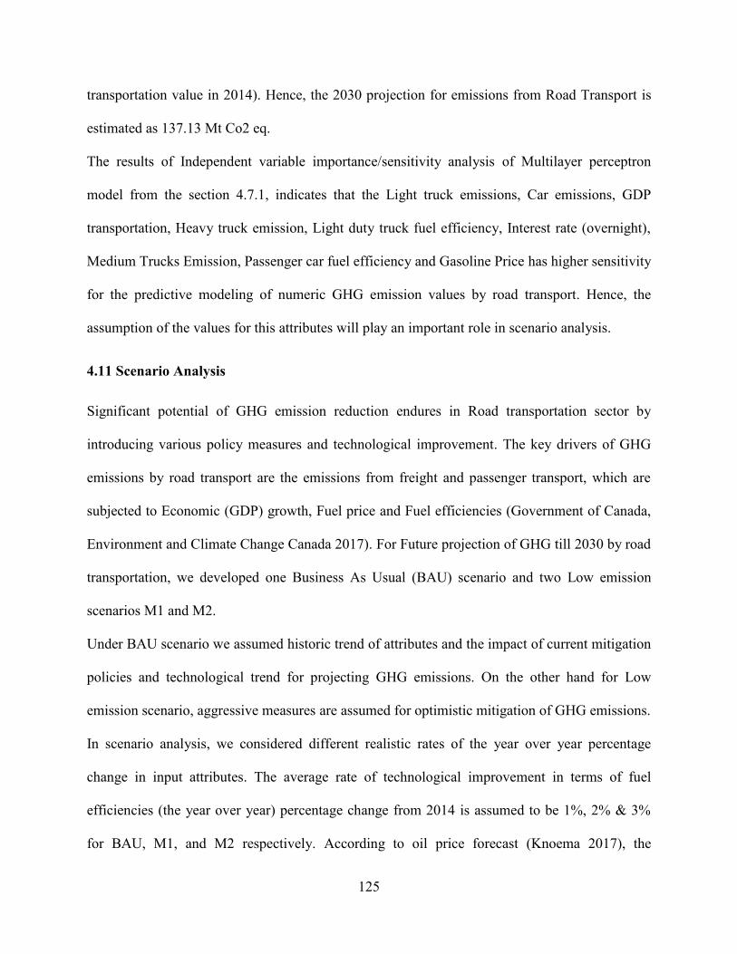
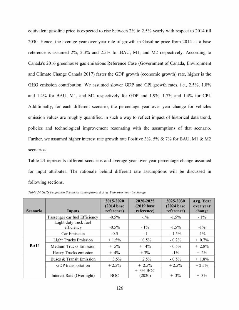
Table 23. Independent Variable Importance ............................................................................... 123 Table 24 GHG Projection Scenarios assumptions & Avg. Year over Year % change ............... 126
Page 14
1
Chapter 1
Introduction
1.1 Background
1.1.1 Green House Gases
Commonly referred as GHG are the natural and anthropogenic gaseous constituents of the
atmosphere. They absorb and emit radiations emitted by Earth’s surface, Atmosphere and clouds
at specific wavelengths between spectrums of thermal infrared radiation (Metz et al., 2007). The
intensity of Greenhouse Gases has increased quickly due to the increased anthropogenic
activities along with population progress increasing earth’s temperature. GHG’s absorb the
energy radiated by the sun causing the atmospheric lower part to trap the heat and raise its
temperature this phenomenon is called natural greenhouse gas effect. This natural phenomenon
got amplified since the advent of industrialization and urbanization. The continuous emission of
GHG’s post industrialization has increased its atmospheric concentration subsequently resulting
in global warming and climate change (Wang et al., 1976).
The major greenhouse gases are Carbon dioxide (CO2), methane (CH4), nitrous oxide (N2O),
hydrofluorocarbons (HFCs), sulfur hexafluoride (SF6) and perfluorocarbons (PFCs). Out of
these major gases, the most dominant is CO2 which accounts 77% of global CO2 equivalent
causing global warming (Metz et al., 2007).
1.1.2 Green House Gases Emissions
United Nations Organization established Inter-Governmental Panel on Climate Change (IPCC)
in 1988 and formed United Nations Framework Convention on climate change (UNFCCC) these
Page 15
2
proceedings motivated to quantify the atmospheric concentration of GHG to avoid hazardous
anthropogenic interference with earth’s climate structure. In the year 1997, developed countries
adopted Kyoto Protocol to collectively reduce the emissions of six important GHG gases by
5.2% compared to the level in 1990 during the 2008-2012 period (Breidenich et al., 1998).
These framework and protocol obliged accounting of GHG emissions at regional levels. Carbon
dioxide, nitrous oxide, and methane are major greenhouse gases (GHG).
Carbon dioxide (CO2) emissions: Since the advent and during industrialization era the CO2
emission level has exponentially increased from 280 ±20 (estimated level between last 10,000
years and 1750) (Delmas et al., 1980) (Indermühle et al., 1999) to 367 ppm in 1999 (Griggs et
al., 2002) and 379ppm in 2005 (Houghton et al., 2001). In 2016 the CO2 emissions have crossed
400 ppm.
Methane (CH4) emissions: It is estimated that human related activities such as biomass
burning, fossil fuel production, manure management, rice cultivation, fermentation in livestock
and waste management release more than 50% of CH4 global emission (Anderson et al., 2010).
The constant increase in CH4 emissions during the 20th
century resulted in 1745 ppb emission
value in 1998 (Houghton et al., 2001) and 1774 ppb in 2005 (IPCCEggleston et al., 2006).
Nitrous oxide (N2O) emissions: Concentration of N2O has a slow increase during the industrial
revolution from 314 ppb in 1998 to 319 ppb in 2005 (Houghton et al., 2001). The sources of
N2O are both natural and anthropogenic activities like Sewage treatment, animal manure
Page 16
3
management, agriculture soil management, combustion of nitric acid & fossil fuels and
biological sources (microbial action) in soil and water (Anderson et al., 2010).
1.1.3 Green House Gases effects
Growing concentration of GHG gases in the atmosphere is raising earth’s temperature. This
steady rise in temperature will lead to forthcoming catastrophic conditions like a change in
climate cycle and melting of ice glaciers leading to rising in sea levels (Wang et al., 1976). There
are environmental, health and economic impacts of greenhouse gas emissions like Coastal
flooding, increase in precipitation levels, flooding, forest fires as a result of increase heat wave,
Increase in diseases and invasive species within wild life, heat strokes, health problems because
of air pollution, economic impact on agriculture, forestry, tourism and recreation because of
changing weather pattern and infrastructure damage and (Government of Canada, Environment,
2016).
1.2 Context of Study
Climate change and global warming are likely to lead to more extreme weather events as well as
harvest failures and rising sea levels, all of which cause enormous damage and economic loss.
Since industrialization began in the 19th century, annual GHG emissions have been increasing
steadily, and a turning point is not in sight (Marland et al., 2003).
Greenhouse gases trap heat in the Earth's atmosphere. Human activities increases the amount of
GHGs in the atmosphere, contributing to a warming of the Earth's surface. In Canada the
national indicator tracks seven GHGs, carbon dioxide (CO2), methane (CH4), nitrous oxide
(N2O), sulphur hexafluoride (SF6), perfluorocarbons (PFCs), hydrofluorocarbons (HFCs) and
Page 17
4
nitrogen trifluoride (NF3) (Government of Canada, Environment and Climate Change Canada
2017) released by human activity (reported in Mt CO2 eq) (United Nations Framework
Convention on Climate Change 2017)
The Kyoto Protocol and (UNFCC) United Nation Framework Convention on Climate Change
initiated the first global effort in GHG emission reduction. To achieve significant sustainable
emission reduction, all the involved countries need suitable methods and models to calculate
their respective emission data and thereby trends.
Emission inventories, which are collections of huge number and variants of input parameters, are
the main sources of GHG emissions. Depending on the emission model used, these parameters
are distinctly harnessed to aid the calculations.
In Canada, transportation is the second largest contributor to the GHG emissions and road
transport has the greatest GHG footprint of the transport sector and recently reducing it is the
main priority of sustainable transport policies.
1.4 Contribution of the Study
In this thesis, we present an alternative method for modeling and predicting GHG Emissions
specifically from Road transportation (passenger and freight).
The models are developed using machine learning approach because:
The models learn the relationship between inputs and outputs by adapting and capturing
historical data and the underlying functional relationship.
With the help of learning on historical data, future predictions are performed on unseen
data set.
Page 18
5
Machine learning models compared to traditional inventory based models are less complex, need
a small number of inputs, minimal in depth field knowledge and most notably inputs are not
predetermined as compared to traditional (COPERT, MOVES, and GAINS) models. The
existing road traffic emissions prediction models require a set of predefined input variables
(generally, emission factor (EF) and activity rate (A)) which are sometimes difficult to discover.
The best performing model (Multilayer Perceptron with Bagging) proposed in the thesis is
flexible, and regional and provincial governments can utilize its variant as well as developing
and developed countries, by employing the relevant inputs available at their discretion for GHG
Emission predictions. Further, simulations can be performed on the developed model to analyze
changes in future projections by introducing relevant changes in inputs resonating with the
policy implications.
In this thesis, we implemented model performance improvement techniques (ensemble learning)
on the best performing machine learning model to further improve its performance. This is a
novel approach which has not been utilized in the context of GHG emissions projections by road
transportation before.
The traditional models like COPERT, MOVES, and GAINS used for GHG emissions evaluation
give emission values of a specific pollutant as output. The model proposed in this thesis is
designed to predict overall values of Canadian GHG emissions specifically by Road transport
using Socio-economic, demographic & emission input data.
1.3 Thesis Objectives/Thesis Statement
The objective of this research is to undertake the study of data mining/machine learning models
to predict the GHG emission caused by road transportation in Canada. The focus is on projecting
Page 19
6
GHG emission values by considering the impact of historical data trend, current & potential
future technology and policy measures adopted by provincial and Federal Government on
socioeconomic, demographic & emission input data. Ensemble learning techniques are
implemented to boost performance improvement of algorithm followed by variable importance
analysis to identify the sensitive input parameter to the model respectively
Furthermore, different scenarios projection given by best performing supervised machine
learning model are assessed and additional policy measures echoing with current and future
policy proposed by the federal and provincial government, to mitigate GHG emissions caused by
road transportation in Canada are investigated. The following tasks are undertaken to achieve the
objectives of our thesis:
1. In depth analysis of GHG emissions in Canada and its provinces with a special focus on
GHG emission by Road Transport (passenger & freight).
2. Identifying the most influencing parameter (Feature selection) among the available
socioeconomic, demographic & emission indicators for efficient and accurate GHG
prediction.
3. Implementing Regression and Classification supervised machine-learning algorithms and
analyzing their performances.
4. Improving the performance of best performing supervised machine-learning model using
ensemble technique.
5. Conducting Independent variable importance analysis/sensitivity analysis to test the
robustness of the model and to understand the relationship between input factors and
GHG emissions by road transport.
Page 20
7
6. Conducting Scenario Analysis and projecting GHG Emissions by road transportation for
each scenario till the year 2030 by considering historical trend, technological
improvement, current federal & provincial policy measures and potential policies to be
introduced in future. Concerning the findings, new policy suggestions to mitigate GHG
Emissions by constituents of road transport are echoed.
1.5 Thesis Organization
The rest of the report is organized as follows:
Chapter 2 presents literature review. Traditional methods to evaluate GHG emissions & their
limitations are outlined. Further, research gap is discussed.
Chapter 3 presents the methodology of data mining and machine learning algorithms and
performance improvement algorithms (ensemble techniques).
Chapter 4 presents the application of research methodology and GHG emission future
projections and scenario analysis for Canadian road transport through 2030.
Chapter 5 presents conclusions and future scope of this research.
Page 21
8
Chapter 2
Literature Review
2.1 Methods to Evaluate GHG emissions
The main source of GHG emission data is GHG inventories (National Inventory Submissions
2017). These inventories contain a large number of input parameters, which are used to calculate
total emissions. Each model uniquely utilizes this parameter to determine the final emission total.
Most emission sectors like Oil and Gas, Electricity, Transportation, Heavy Industry, Buildings,
etc. are the product of a statistical parameter of the respective source, i.e., Activity data (A) and
an Emission factor (EF) (Winiwarter et al., 2001).
𝐺𝐻𝐺 𝐸𝑚𝑖𝑠𝑠𝑖𝑜𝑛𝑠 = 𝐴𝑐𝑡𝑖𝑣𝑖𝑡𝑦 𝑑𝑎𝑡𝑎 × 𝐸𝑚𝑖𝑠𝑠𝑖𝑜𝑛 𝑓𝑎𝑐𝑡𝑜𝑟
Where:
Activity data refer to the estimated quantitative amount of human activity resulting in emissions
during a given time period E.g. The total amount of fossil fuel burned is the activity data for
fossil fuel combustion sources (Government of Canada, Environment and Climate Change
Canada 2017).
The emission factor is the average emission rate of a given GHG for a given source, relative to
units of activity. It relates the quantity of a pollutant released to the atmosphere with an
associated activity. Emission factors are generally expressed as the weight of pollutant divided
by a unit weight, volume, distance, or duration of the activity emitting the pollutant (United
Page 22
9
States Environmental Protection Agency 2016), e.g., Kilograms of particulate emitted per mega
gram of coal burned.
2.1.1 Road Transport Emission Inventory Models
In this section, we will discuss the most commonly used inventory models namely COPERT and
MOVES, which provide estimates of road transport emissions.
COPERT
COPERT (Computer Programme to Calculate Emissions from Road Transport) is European
Road Transport Emission Inventory Model. It is a software tool used worldwide to calculate air
pollutant and greenhouse gas. The development of COPERT is coordinated by the European
Environment Agency (EEA) (Dimitrios et al., 2012).
COPERT estimates emissions from road transport. The program estimates quantities of GHG
emissions; carbon dioxide (CO2), methane (CH4), nitrous oxides (N2O) and local emissions;
carbon monoxide (CO), nitrogen oxides (NOx), non-methane volatile organic compounds
(NMVOC), PM, and fuel-related emissions such as lead (Pb) and sulphur dioxide (SO2 ), which
are emitted from road transport vehicles (passenger cars, light duty vehicles, heavy duty vehicles,
mopeds and motorcycles) (Ren et al., 2016).
COPERT model is an average speed model (XIE et al., 2006). COPERT is based on the driving
cycle named NEDC (New European Driving Cycle) and the calculation of emission factors
depends on fixed driving cycle (Dimitrios et al., 2012). COPERT calculates the emissions
separately for urban, rural, and highway driving modes. The cold-start emissions are identified to
the urban driving mode, and hot emissions are recognized to rural and highway driving modes.
In cases, where the distance driven during the cold-start period is over the urban trip distance,
Page 23
10
portions of the cold-start emissions are recognized to rural driving. Also, the program considers
evaporative emissions for gasoline-fueled vehicles. The calculation is given by below Equation
as follows (Soylu, 2007). (Sun et al., 2016):
𝐸𝑇𝑜𝑡𝑎𝑙 = 𝐸𝑈𝑟𝑏𝑎𝑛 + 𝐸𝑟𝑢𝑟𝑎𝑙 + 𝐸𝐻𝑖𝑔ℎ𝑤𝑎𝑦
Where:
𝐸𝑈𝑟𝑏𝑎𝑛,𝐸𝑟𝑢𝑟𝑎𝑙, and 𝐸𝐻𝑖𝑔ℎ𝑤𝑎𝑦 are the emissions of pollutants for the appropriate driving mode.
The products of the driving mode activity data and the relevant emission factors give the quantity
of the driving mode emissions.
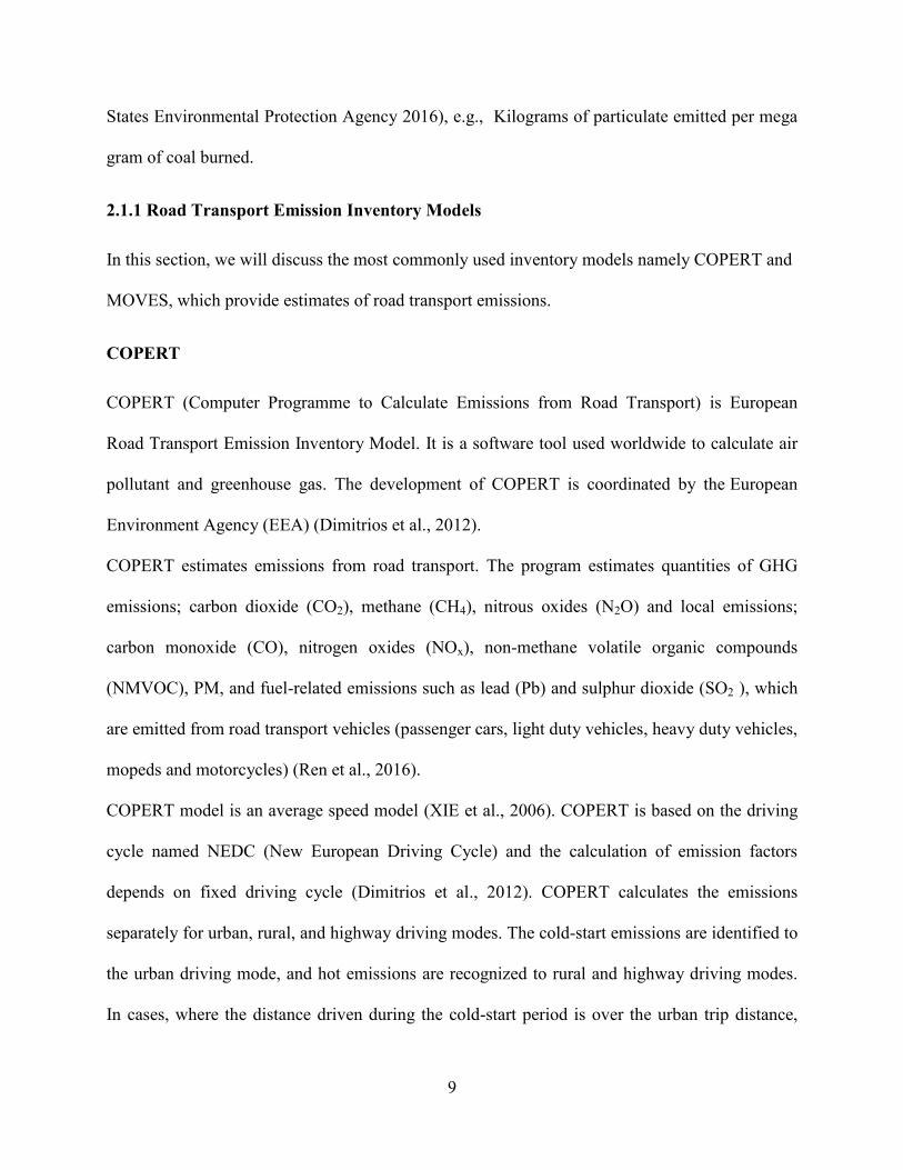
Figure 1 shows the following data required as input for the calculations:
Figure 1. Required input data for COPERT model (Source: Dimitrios et al., 2012).
(1 & 2) Meteorological data
(3) Fuel consumption for the road transport.
(6) The maximum and minimum ambient temperatures (monthly average).
(4 & 5) Fleet data (number of vehicles in each category).
Also, also, it requires (Song et al., 2016).
The official date of introduction of the emission regulations
Page 24
11
Mileage distribution (urban, rural, highway) and average vehicle speeds.
The understanding of any study using COPERT has been highly sensitive to the possibility of
obtaining reliable estimations of the input data (Burón et al., 2004).
Once the input data are ready, the program can be run for nationwide estimation of the emissions
on a yearly basis.
Mobile 6.2 model and Motor Vehicle emission simulator (Moves)
The US EPA used the MOBILE model in the past to estimate the vehicle emission factors for
regulatory purposes. The MOBILE6.2 model (the latest version in the MOBILE series) is a fuel
based emission factor model that broadly classifies vehicles into gasoline motorcycles, diesel,
and gasoline powered cars, trucks and buses (Kota et al., 2014). Recently, the US EPA replaced
the MOBILE6.2 model with the MOVES (Motor Vehicle Emission Simulator) model (U.S.
Environmental Protection Agency, 2012) as the official model for estimating on-road vehicle
emissions.
MOVES model is designed to work with databases. In this model, new data may become
available and can be more easily incorporated into the model (U.S. Environmental Protection
Agency, 2012). The free access database structure provides convenience for modifying emission
data in MOVES (Liu et al., 2013).
MOVES applies the relationship between vehicle specific power (VSP) and emissions and then
establishes the emission rates database based on VSP. It uses the distribution of VSP to describe
vehicle-operating modes, which is more flexible than COPERT and MOBILE who are based on
fixed driving cycles. Furthermore, in MOVES, operating modes are binned according to second-
by-second speed and VSP (Vallamsundar et al., 2011).
Page 25
12
MOVES uses an activity based approach and classifies vehicles based on their utilities
(passenger cars, passenger trucks, light commercial trucks, refuse trucks, single unit short-haul
trucks, single unit long-haul trucks, combination short-haul trucks, combination long-haul trucks,
motorcycles, motor homes, and buses) (U.S. Environmental Protection Agency, 2012). In this
model, each vehicle type can be combined with one of several fuel types (diesel, gasoline,
natural gas, electric, etc.) to estimate their emission factors (Kota et al., 2014). MOVES include
both regional emission component to support the development of national and regional emission
inventories and project-level emission component to support local-scale emission and air quality
modeling (Kota et al., 2014).
2.2 Other Emission Inventory Models
In this section the model GAINS is discussed which calculates generalized emission inventories
by bringing together information on future economic, energy and agricultural development,
emission mitigation potentials and costs, atmospheric dispersion and environmental sensitivities
towards air pollution (GAINS EUROPE, 2013).
GAINS (Gas and Air pollution Interactions and synergies)
GAINS (GAINS EUROPE, 2013) estimates current and future emissions based on activity data,
uncontrolled emission factors, the removal efficiency of emission control measures and the
extent to which such measures are applied.
The model reports threats to human health by fine particles and ground-level ozone, and
potential risks posed by acidification, nitrogen deposition (eutrophication) and exposure to
elevated levels of ozone. These impacts are considered in a multipollutant context, quantifying
Page 26
13
the contributions of all major air pollutants as well as the six greenhouse gases considered in the
Kyoto protocol (Amann et al., 2011) (GAINS EUROPE, 2013).
The current and future emissions are estimated according to below equation by varying the
activity levels along with external factors projections of anthropogenic driving forces and by
adjusting the implementation rates of emission control measures (Amann et al., 2011).
𝐸𝑖,𝑝 = ∑ ∑ 𝐴𝑖,𝑘𝑚
𝑒𝑓𝑖,𝑘,𝑚,𝑝 𝑥𝑖,𝑘,𝑚,𝑝𝑘
Where:
𝑖, 𝑘, 𝑚, 𝑝 - Represents Country, activity type, abatement measure, pollutant, respectively.
𝐸𝑖,𝑝 - Emissions of pollutant p (for SO2, NOx, VOC, NH3, PM2.5, CO2, CH4, N2O, F-gases) in
country i.
𝐴𝑖,𝑘 - Activity level of type k (e.g., coal consumption in power plants) in country i.
𝑒𝑓𝑖,𝑘,𝑚,𝑝 - Emission factor of pollutant p for activity k in country i after application of control
measure m.
𝑥𝑖,𝑘,𝑚,𝑝 - Share of total activity of type k in country i to which a control measure m for pollutant p
is applied.
2.3 Limitations of the models used to evaluate road transport GHG emissions
To implement effective policies to mitigate road transport emissions, determination of pollutant
emissions from transport sector is the first step. Upon providing sufficiently reliable input, data
emission inventory models such as COPERT and MOVES can provide reliable estimates of road
transport emissions. For policy makers to make a better decision for future a set of well-defined
input parameters is a must and preparation of detailed statistical data for different vehicle
Page 27
14
categories, and their unique operating conditions are challenging to be overcome (Burón et al.,
2004) (Saija et al., 2002).
Page 28
15
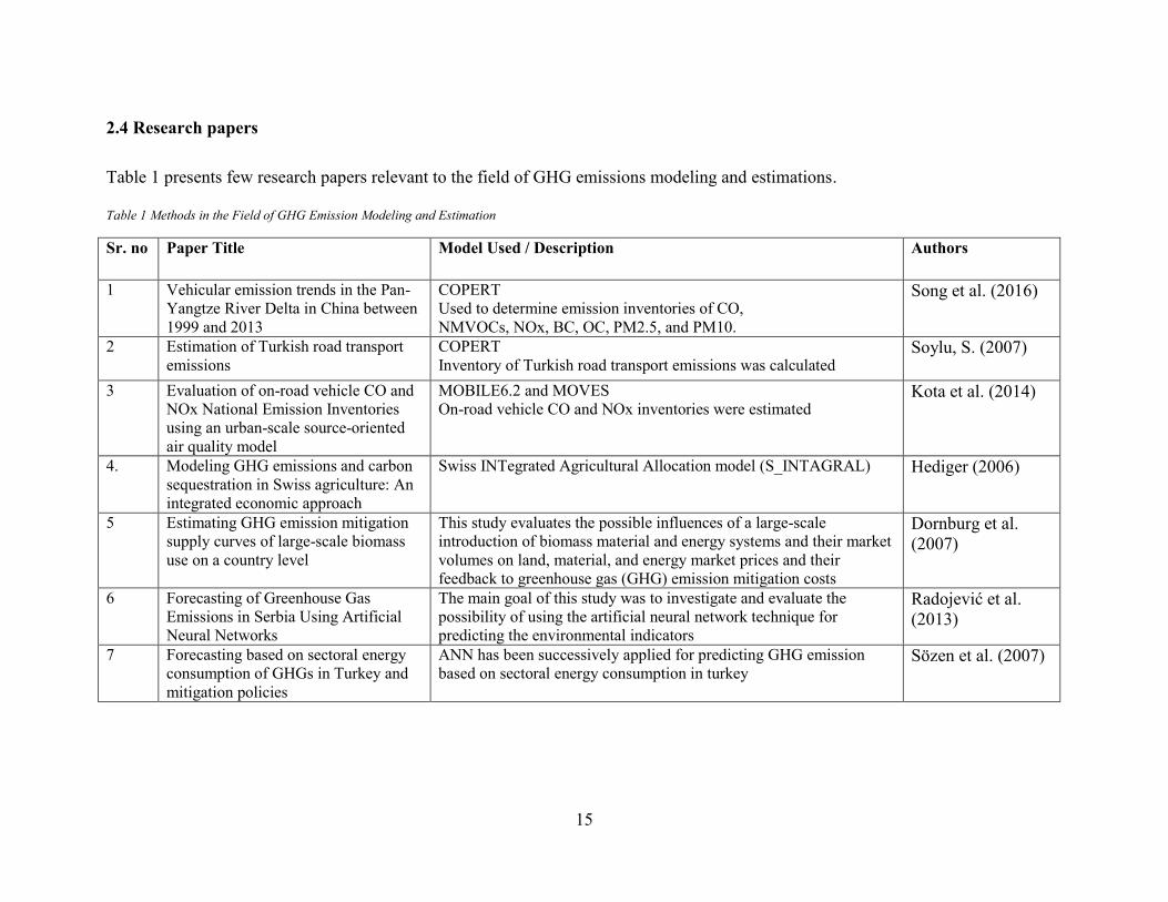
2.4 Research papers
Table 1 presents few research papers relevant to the field of GHG emissions modeling and estimations.
Table 1 Methods in the Field of GHG Emission Modeling and Estimation
Sr. no Paper Title Model Used / Description Authors
1 Vehicular emission trends in the Pan-
Yangtze River Delta in China between
1999 and 2013
COPERT
Used to determine emission inventories of CO,
NMVOCs, NOx, BC, OC, PM2.5, and PM10.
Song et al. (2016)
2 Estimation of Turkish road transport
emissions
COPERT
Inventory of Turkish road transport emissions was calculated Soylu, S. (2007)
3 Evaluation of on-road vehicle CO and
NOx National Emission Inventories
using an urban-scale source-oriented
air quality model
MOBILE6.2 and MOVES
On-road vehicle CO and NOx inventories were estimated Kota et al. (2014)
4. Modeling GHG emissions and carbon
sequestration in Swiss agriculture: An
integrated economic approach
Swiss INTegrated Agricultural Allocation model (S_INTAGRAL) Hediger (2006)
5 Estimating GHG emission mitigation
supply curves of large-scale biomass
use on a country level
This study evaluates the possible influences of a large-scale
introduction of biomass material and energy systems and their market
volumes on land, material, and energy market prices and their
feedback to greenhouse gas (GHG) emission mitigation costs
Dornburg et al.
(2007)
6 Forecasting of Greenhouse Gas
Emissions in Serbia Using Artificial
Neural Networks
The main goal of this study was to investigate and evaluate the
possibility of using the artificial neural network technique for
predicting the environmental indicators
Radojević et al.
(2013)
7 Forecasting based on sectoral energy
consumption of GHGs in Turkey and
mitigation policies
ANN has been successively applied for predicting GHG emission
based on sectoral energy consumption in turkey Sözen et al. (2007)
Page 29
16
2.5 Research Gap
The Literature review and cited research papers provide insightful information about road
transportation emissions inventory models and neural network models for GHG emissions
prediction. Also, to the best of our knowledge, it was found that no in-depth studies have been
conducted in regards to distribution of GHG emission future projections by road transportation in
Canada, and no ensemble techniques have been utilized for improving machine learning models
performances for road transport GHG emissions modeling.
In Table 1 the mentioned research studies using road transport emission models are extensively
focused on estimating vehicle emissions inventory by considering only freight relevant and
meteorological data for, eg. Vehicle types, fuel type, driving speed, etc. Many research papers
focused on only calculating emission factors using several emission monitoring and inventorying
tools such as (COPERT and MOVES) to calculate the emission with respect to region, vehicle
type, etc. while others just focused on forecasting overall GHG emissions (at country level) using
simple neural networks.
In general, most of the emission sectors are estimated by multiplying the emission factor (EF)
with the activity rate (A), a statistical parameter for the respective source. In practice, none of the
input parameters (EF or A) is exactly known. In an emission inventory, the values of the
parameters are determined as best “estimates” (Winiwarter et al., 2001). The review of the above
papers points out that a limited number of studies have been done on the topic of Road transport
GHG emissions by using data mining & machine learning models and independent & widely
available indicators for, eg. Socioeconomic parameters, emission data, fuel efficiency, etc.,
compared to pre-determined input variables.
Page 30
17
Compared to inventory based models, machine-learning models are less complex, requires fewer
input parameters and does not require pre-determined parameters and hence these models can be
implemented and assessed for GHG emission predictive modeling using available parameters. In
addition to our study the data sources in Canada are widely available and grant access to relevant
activity/emission input parameters needed for the machine learning models, we can use such a
model for predicting Road transport GHG emissions.
Page 31
18
Chapter 3
Methodologies
3.1 Feature Selection
It is also known as attribute or variable selection in machine learning and statistics. It is used to
detect relevance among the features and help in distinguishing irrelevant, redundant, or noisy
variable data.
Feature selection method helps in achieving the following aims (Shardlow, 2016):
To reduce the size of the problem - reducing compute time and space required to run
machine learning algorithms.
To improve the predictive accuracy of classifiers. Firstly by removing noisy or irrelevant
features. Secondly by reducing the likelihood of over fitting to noisy data
To identify which features may be relevant to a specific problem.
Unrelated features provide no useful information, and redundant features provide no more
information than the presently selected features (Manikandan et al., 2015). Feature selection is
one of the most frequent and important techniques in data preprocessing and has become a
necessary component of the machine learning process (Kalousis et al., 2007).
In our research, we implemented filter method for feature selection using WEKA’s attribute
evaluator and search method to determine set of relevant input indicators among the field of
socio-economic, demographic and emission data.
Page 32
19
WEKA (Waikato Environment for Knowledge Analysis)
It is free software used widely in the field of data mining, business, and machine learning. It
inhibits algorithms for predictive modeling and data analysis, with a GUI for easy access to those
functions. WEKA is competent to assess in data preprocessing, clustering, classification,
visualization, and feature selection (Witten et al., 2016).
3.1.1 Relief Attribute Evaluator
The Relief algorithm was first described by Kira and Rendell (Kira et al., 1992), it is an effective
method to attribute weighing.
Feature selection has been used widely to determine the quality of the attributes to be used for
analysis with the help of machine learning algorithms for either classification or regression. In
case of feature selection Relief algorithms (Relief, ReliefF, and RReliefF) are efficient and can
correctly estimate the quality of attributes in a given experiment and considers strong
dependencies among attributes (Robnik-Šikonja et al., 2003). Relief algorithms are commonly
considered for feature selection method before applying any learning. According to (Dietterich,
1997), Relief algorithms are one of the most successful pre-processing algorithms. Relief
algorithms have been used as an attribute weighting method (Wettschereck et al., 1997) and
feature selection for price forecasting (Amjady et al., 2008).
The original Relief algorithm (Kira et al., 1992) was limited to classification problems with two
classes. The extension of Relief, i.e., ReliefF that was able to perform more efficiently in the
presence of noise and missing data was given by (Kononenko, 1994). It can also deal with the
multi-class problem. Further, in the year 1997, (Robnik-Šikonja et al., 1997) improved the
algorithm for its adoption to continuous (numeric) class values. In our research, for feature
Page 33
20
selection, we used the numeric value of our dependent variable GHG emission by road transport.
In the below section we will have an overview of the RReliefF algorithm.
Basic Relief Algorithm
The output of the Relief algorithm is a weight between −1 and 1 for each attribute, with more
positive weights indicating more predictive attributes (Rosario et al., 2015).
According to (Kira et al., 1992), the basic idea of Relief algorithm is to estimate the quality of
attributes. Relief’s estimate of the quality of weight W [A] is an approximation of following
differences of probabilities (Kononenko, 1994).
W [A] = P (diff. value of A | nearest inst. From diff. class) - P (diff. value of A | nearest inst.
from same class) – (Equation 1)
The attribute weight estimated by Relief has a probabilistic interpretation. It is proportional to
the difference between two conditional probabilities, namely, the probability of the attribute’s
value being differently conditioned on the given nearest miss and nearest hit respectively
(Robnik-Šikonja et al., 1997)
Pseudo code: Relief Algorithm (Robnik-Šikonja et al., 1997):
Input: for each training instance a vector of attribute values and the class value
Output: the vector W of estimations of the qualities of attributes
1. Set all weights W [A] = 0.0;
2. for i := 1 to m do begin
3. randomly select an instance 𝑅𝑖;
4. find nearest hit H and nearest miss M;
5. for A = 1 to a do
Page 34
21
6. W[A] = W[A] – diff (A, 𝑅𝑖, H)/m + diff(A, 𝑅𝑖, M)/m;
7. end;
In Relief algorithm, The positive updates of weight (+ diff(A, 𝑅𝑖, M)/m;) are establishing the
probability estimate that the attribute discriminates between instances with different class values
and the negative updates of weight (– diff (A, 𝑅𝑖, H)/m) are establishing the probability estimate
that the attribute discriminates and separate instances with same class value.
RReliefF Algorithm
RReliefF algorithm deals with continuous/numerical predicted value. In such problems with
numeric predictive value nearest hits and misses and hence the knowledge of whether two
instances belong to the same class or different class is useless. To resolve this, the probability
that the predicted values of two instances are different is introduced. With the help of relative
distance between predicted (class) values of two instances, this probability can be modeled.
As W[A] is estimated by the contribution of Positive and negative weight terms, in the
continuous predicted class value problem these terms are missing (where hits end and misses
start). Hence to overcome it the equation 1 can be modified as (Robnik-Šikonja et al., 1997):
W[A] = 𝑃𝑑𝑖𝑓𝑓𝐶|𝑑𝑖𝑓𝑓𝐴𝑃𝑑𝑖𝑖𝑓𝐴
𝑃𝑑𝑖𝑓𝑓𝐶−
(1−𝑃𝑑𝑖𝑓𝑓𝐶|𝑑𝑖𝑓𝑓𝐴) 𝑃𝑑𝑖𝑓𝑓𝐴
1−𝑃𝑑𝑖𝑓𝑓𝐶
Where:
𝑃𝑑𝑖𝑖𝑓𝐴 = P (different value of A | nearest instances)
𝑃𝑑𝑖𝑓𝑓𝐶 = P (different prediction | nearest instances)
Page 35
22
And 𝑃𝑑𝑖𝑓𝑓𝐶|𝑑𝑖𝑓𝑓𝐴 = P (diff. prediction | diff. value of A and nearest instances)
Pseudo code: RReliefF Algorithm (Robnik-Šikonja et al., 1997):
Input: for each training instance a vector of attribute values x and predicted value τ(x)
Output: vector W of estimations of the qualities of attributes
1. set all NdC, NdA[A], NdC&dA[A], WA to 0;
2. for I = 1 to m do begin
3. randomly select instance 𝑅𝑖;
4. select k instances 𝐼𝑗 nearest to 𝑅𝑖;
5. for j = 1 to k do begin
6. 𝑁𝑑𝐶 = 𝑁𝑑𝐶 + diff (𝜏(. ), 𝑅𝑖, 𝐼𝑗).d(i,j);
7. for A = 1 to a do begin
8. 𝑁𝑑𝐴[𝐴] = 𝑁𝑑𝐴[𝐴] + diff (𝐴, 𝑅𝑖, 𝐼𝑗). d(i,j);
9. 𝑁𝑑𝐶&𝑑𝐴[𝐴] = 𝑁𝑑𝐶&𝑑𝐴[𝐴] + diff (𝜏(. ), 𝑅𝑖, 𝐼𝑗).
10. diff (𝐴, 𝑅𝑖, 𝐼𝑗). d(i,j);
11. end;
12. end;
13. end;
14. for A= 1 to a do
15. 𝑊𝐴 = 𝑁𝑑𝐶&𝑑𝐴[𝐴]/ 𝑁𝑑𝐶 - (𝑁𝑑𝐴[𝐴] - 𝑁𝑑𝐶&𝑑𝐴[𝐴]/(m- 𝑁𝑑𝐶)
Alike Relief, the algorithm select random instance 𝑅𝑖 (line 3) and its K nearest instance 𝐼𝑗 (line
4). The weight for different prediction value 𝜏(. ) is collected in 𝑁𝑑𝐶 (line 6)
Page 36
23
The weight for different attribute is collected in 𝑁𝑑𝐴[𝐴] (line 8). The weight for different
prediction and different attribute is collected in 𝑁𝑑𝐶&𝑑𝐴[𝐴] (line 9). The final estimation of each
attribute is given by 𝑊𝐴 = 𝑁𝑑𝐶&𝑑𝐴[𝐴]/ 𝑁𝑑𝐶 - (𝑁𝑑𝐴[𝐴] - 𝑁𝑑𝐶&𝑑𝐴[𝐴]/(m- 𝑁𝑑𝐶) (line 15).
The term d(i,j) = 𝑒− (𝑟𝑎𝑛𝑘 ( 𝑅𝑖,𝐼𝑗)
𝜎)2
The term d(i,j) is exponentiated and decreased (-) to avoid the influence of Ij with the distance
from given instance Ri as the motivation behind this measure is that closer instances will have
greater influence.
Where:
𝑟𝑎𝑛𝑘 ( 𝑅𝑖, 𝐼𝑗) is the rank of instance 𝐼𝑗 in a sequence of instances ordered by the distances from
𝑅𝑖 and 𝜎 is a user defined parameter to control the influence of the distance.
To get a probabilistic reading of results, the contribution of each k nearest instance is
normalized, by dividing it by the sum of all K contributions. The ranks are used to make sure that
the nearest instances always have the same impact on weights (Robnik-Šikonja et al., 1997).
3.2 Data Mining
Data mining is about explaining the past and predicting the future using data analysis and
modeling. It is a multi-disciplinary domain which combines statistics, machine learning and
database technology (Sayad 2011). The most significant application of data mining is machine
learning. Human beings frequently make a mistake when trying to create a relationship between
a set of multiple attributes or potentially during analysis of those attributes. Potential hindrances
are created while finding a solution to a problem involving those variables. In such situation,
Page 37
24
machine learning can often be successfully applied to these problems thereby improving designs
and efficiency of the system (Ayodele, T 2010).
3.2.1 Supervised Learning
Supervised learning is based on training a data sample from a data source with correct
classification already assigned or in other words; then the learning is called supervised. In
supervised learning instances within a dataset can be represented as independent and target
attributes. The kind of modeling depends on the target attribute if the target is discrete the
modeling is classification, but if the target is continuous, the modeling is a regression (Sathya et
al., 2013) (Ayodele, T 2010).
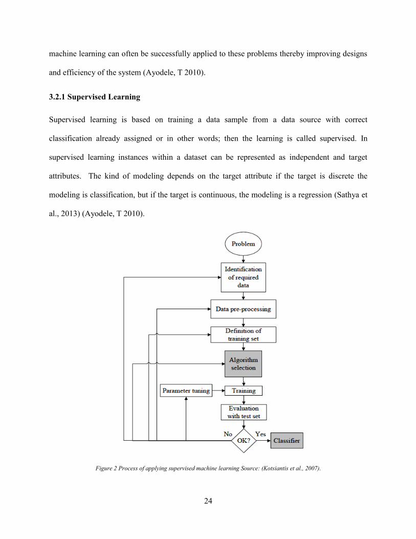
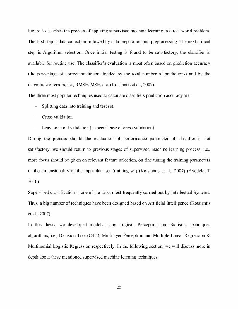
Figure 2 Process of applying supervised machine learning Source: (Kotsiantis et al., 2007).
Page 38
25
Figure 3 describes the process of applying supervised machine learning to a real world problem.
The first step is data collection followed by data preparation and preprocessing. The next critical
step is Algorithm selection. Once initial testing is found to be satisfactory, the classifier is
available for routine use. The classifier’s evaluation is most often based on prediction accuracy
(the percentage of correct prediction divided by the total number of predictions) and by the
magnitude of errors, i.e., RMSE, MSE, etc. (Kotsiantis et al., 2007).
The three most popular techniques used to calculate classifiers prediction accuracy are:
– Splitting data into training and test set.
– Cross validation
– Leave-one out validation (a special case of cross validation)
During the process should the evaluation of performance parameter of classifier is not
satisfactory, we should return to previous stages of supervised machine learning process, i.e.,
more focus should be given on relevant feature selection, on fine tuning the training parameters
or the dimensionality of the input data set (training set) (Kotsiantis et al., 2007) (Ayodele, T
2010).
Supervised classification is one of the tasks most frequently carried out by Intellectual Systems.
Thus, a big number of techniques have been designed based on Artificial Intelligence (Kotsiantis
et al., 2007).
In this thesis, we developed models using Logical, Perceptron and Statistics techniques
algorithms, i.e., Decision Tree (C4.5), Multilayer Perceptron and Multiple Linear Regression &
Multinomial Logistic Regression respectively. In the following section, we will discuss more in
depth about these mentioned supervised machine learning techniques.
Page 39
26
Multiple Linear Regression
When the outcome of a problem is numeric and all input attributes are continuous linear
regression is deployed frequently (Zou et al., 2003). The purpose of linear regression analysis is
to evaluate the relative impact of a predictor variable on a particular outcome. Regression with
the single attribute is called as simple linear regression and regression with multiple attributes is
called as multiple linear regression. The Linear regression serves as building blocks of complex
learning methods (Witten et al., 2016).
Linear Regression helps in the easy fitting of models, which depends linearly on their attributes.
Linear Regressions are extensively used statistical tool in various practical applications majority
of them being forecasting and predictive modeling (Yan et al., 2009)
Considering a given data set { 𝑦𝑖, 𝑥𝑖1, 𝑥𝑖2, … , 𝑥𝑖𝑘} where i = 1 to n. The linear Regression model
is given by (Lang, H. 2013):
𝑦𝑖 = 𝛽0 + 𝑥𝑖1𝛽1 + 𝑥𝑖𝑘𝛽𝑘 + 𝑒𝑖
Where 𝑖 = 1,2,3. . 𝑛
𝑦𝑖 – Dependent variable
𝑥𝑖𝑘 – Independent variable for the Dependent variable 𝑦𝑖
𝛽𝑘 – Unknown parameters (to be estimated from data)
𝑒𝑖 – Error term
The regression equation can also be denoted in the matrix form for convenience:
𝑌 = 𝑋𝛽 + 𝑒
𝑌 𝑖𝑠 𝑎 𝑛 × 1 vector:
Page 40
27
Y = (
y1
⋮yn
)
𝑋 𝑖𝑠 𝑎 𝑛 × (𝑘 + 1) matrix:
X = 1 𝑥𝑖1
⋮ ⋮1 𝑥𝑛1
⋯ 𝑥𝑖𝑘
⋱ ⋮… 𝑥𝑛𝑘
𝛽 𝑖𝑠 (𝑘 + 1) × 1 vector:
β = (β0
⋮βk
)
𝑒 𝑖𝑠 𝑛 × 1 vector:
e = (
e1
⋮en
)
The values for unknown parameters will be calculated using training data. Let's say the first
instance will have a dependent variable value 𝑦1 and independent variable values as
𝑥11, 𝑥12, … . , 𝑥1𝑘, where the subscript value 1 denotes it’s a first example.
The predicted value for a first instance dependent variable can be written as (Witten et al., 2016):
𝑥10𝛽0 + 𝑥11𝛽1 + 𝑥12𝛽2 + 𝑥1𝑘𝛽𝑘 = ∑ 𝑥1𝑘𝛽𝑘
𝑘
𝑗=0
The difference between the predicted and the actual value is vital in linear regression. The core
of Linear Regression methodology is to select the values of unknown parameters 𝛽𝑘 and
𝛽𝑜(constant/offset) to minimize the sum of square errors over all training instances.
Then the sum of squared difference over all training instance is:
∑ 𝑒��2
𝑛
𝑖=1
= ∑(𝑦𝑖 − ∑ 𝑥𝑖𝑘𝛽𝑘
𝑘
𝑗=0
)2
𝑛
𝑖=1
Page 41
28
∑ 𝑒��2
𝑛
𝑖=1
= ∑(𝑦𝑖 − ��)2
𝑛
𝑖=1
Where the expression (𝑦𝑖 − ��) is the difference between the ith example’s actual class and its
predicted class.
Ordinary Least Square Estimation (OLS)
The OLS estimator is considered the optimal estimator of unknown parameters 𝛽 (Kennedy, P.
2008). The estimated �� gained by the application of this method minimizes the sum of square
errors. This is achieved by taking the derivative of sum of square errors with respect to �� and
equating it to zero (Lang 2013).
∑ 𝑒��2
𝑛
𝑖=1
= ∑(𝑦𝑖 − ��)2
𝑛
𝑖=1
= (𝑦 − 𝑋𝛽)𝑇(𝑦 − 𝑋𝛽)
= 𝑦𝑇𝑦 − 𝑋�� − 𝛽��𝑋𝑇𝑦 + 𝛽��𝑋𝑇𝑋��
The derivative with respect to 𝛽:
𝜕(𝑦𝑇𝑦 − 𝑋�� − 𝛽��𝑋𝑇𝑦 + 𝛽��𝑋𝑇𝑋��)
𝜕��= 0
−2𝑋𝑇𝑦 + 2𝑋𝑇𝑋�� = 0
𝑋𝑇𝑦 = 𝑋𝑇𝑋��𝑦
Therefore:
�� = (𝑋𝑇𝑋)−1𝑋𝑇𝑦
The OLS method under multiple linear regression is unbiased and thus 𝐸(��) = 𝛽.
Page 42
29
Multinomial Logistic Regression
Logistic regression also called logit model, is a statistical modeling technique. It evaluates the
relationship between multiple independent variables and categorical dependent variable and
estimates the probability of occurrence of an event by fitting data to a logistic curve. Depending
on the type and value of dependent variable logistic regression can be classified as binary and
multinomial logistic regression models (Hosmer & Lemeshow 2000). Multinomial Logistic
regression is a generalization of logistic regression (Hosmer et al., 2013). Binary logistic
regression is used when the dependent variable is dichotomous, and the independent variables
are either continuous or categorical. When the dependent variable is not dichotomous and is
comprised of more than two categories, a multinomial logistic regression can be employed
(Hosmer et al., 2013) (Park 2013).
The aim of Multinomial logistic regression based supervised learning algorithm is to design a
classifier based on L labeled training samples, that is capable of distinguishing K classes when
feature vector (S) is given as an input for classification (Hosmer et al., 2013).
Today, the logistic regression models are one of the most widely used models in the analysis of
categorical data. There are a lot of research papers available where the function of Logistic was
applied to model population growth, health care situations and Market penetration of new
products and technologies.
The important concept in logistic / multinomial logistic regression is the concept of Odds; Odds
of an event are the ratio of the probability that an event will occur to the probability that it will
not occur. If the probability of an event occurring is p, the probability of the event not occurring
is (1-p). Then the corresponding value of odds is a value given by odds of an event (Park, H.
2013).
Page 43
30
Odds of an Event= 𝑃
1−𝑃
The impact of independent variables is usually explained in terms of odds, as multinomial
logistic regression estimates the probability of an event occurring over the probability of an event
not occurring. The multinomial logistic function is used when the dependent variable has k
possible outcomes. MNL uses a linear predictor function f(k, i) to predict the probability that
observation i has outcome k.
The function can be described as:
f (k,i) = 𝛽0,𝑘 + 𝛽1,𝑘𝑥1,𝑖 + 𝛽2,𝑘𝑥2,𝑖 + ……… + 𝛽𝑀,𝑘𝑥𝑀,𝑖
f (k,i) = 𝛽0,𝑘 + 𝛽𝑘. 𝑋𝑖
Where:
Xi, is the set of independent variable
βk, is set of regression coefficients associated with outcome k
Unfortunately, the probability given by this function is not a good model because extreme values
of x will give values of 𝛽0,𝑘 + 𝛽𝑘. 𝑋𝑖, and these values does not fall between 0 and 1. The
logistic regression solution to this problem is to transform the odds using the natural logarithm
(Peng et al., 2002).
When there are K possible categories of the response variable, the model consists of k-1
simultaneously logit equation. With multinomial logistic regression we model the natural log
odds as a linear function of the explanatory variable:
Logit (Y) = ln 𝑃𝑟(𝑦𝑖=𝑘−1)
𝑃𝑟(𝑦𝑖=𝑘) = 𝛽0,𝑘 + 𝛽𝑘. 𝑋𝑖
To implement MNL with K possible dependent variable outcomes, one outcome is considered as
baseline category. In the above log odd equation category, K is considered as baseline category.
Page 44
31
In the model, the same independent variable appears in each of K categories and separate
intercept β0,k and slope parameter βk is estimated for each category. The slope parameter
𝛽𝑘 represents the additive effect of a unit increase in the independent variable x, on the log odds
of being in category k-1, rather than the reference category (Wang 2005).
Further to calculate and interpret the effect of an independent variable it is good to take
exponential of both sides of the equation to get predicted probabilities (Wattimena 2014).
𝑃𝑟(𝑌𝑖 = 𝑘 − 1) = 𝑒𝛽𝑘−1.𝑋𝑖
1 + ∑ 𝑒𝛽𝑘.𝑋𝑖𝑘−1𝑘=1
The probability of the reference category, “K” can be calculated as (Wang 2005):
(𝑃𝑟(𝑌𝑖 = 𝑘)) = 1 − (𝑒𝛽𝑘−1.𝑋𝑖
1 + ∑ 𝑒𝛽𝑘.𝑋𝑖𝑘−1𝑘=1
)
Multilayer Perceptron
The most significant invention in the field of soft computing is Neural Networks (NN), inspired
by biological neurons in the human brain. The concepts of Neural Networks were first
mathematically modeled by McCulloch and Pitts (McCulloch et al., 1943). Over the last decade,
the high performance of the mathematical model has made it remarkably popular. The Feed
Forward Neural Network (FNN) is the simplest and most widely used among different types of
NNs (Fine 2006).
Single-Layer Perceptron (SLP) and Multi-Layer Perceptron (MLP) are two types of FNN. The
difference between the two types is the number of Perceptron. SLP has a single perceptron, and
MLP has more than one perceptron. SLP is suitable for solving linear problems (Rosenblatt
Page 45
32
1957) whereas, due to having more than one perceptron, MLPs are proficient of solving
nonlinear problems (Werbos 1974) (McCulloch et al., 1990).
The greatest advantage of Multilayer perceptron (MLPs) is that a priori knowledge of the
specific functional form is not required. MLPs are not only a ‘black box’ tool. In fact, they have
the potential to significantly enhance scientific understanding of empirical phenomena subject to
neural network modeling (Mirjalili et al., 2014). The applications of MLPs are categorized as
pattern classification (Melin et al., 2012), data prediction (Guo et al., 2012), and function
approximation (Gardner et al., 1998), Pattern classification implies classifying data into
predefined discrete classes (Barakat et al., 2013), whereas prediction refers to the forecasting of
future trends according to current and previous data (Guo et al., 2012) and function
approximation involves the process of modeling relationships between input variables.
The MLP model is a flexible and general-purpose type of ANN composed of one input layer, one
or more hidden layers, and one output layer (Dawson et al., 1998).
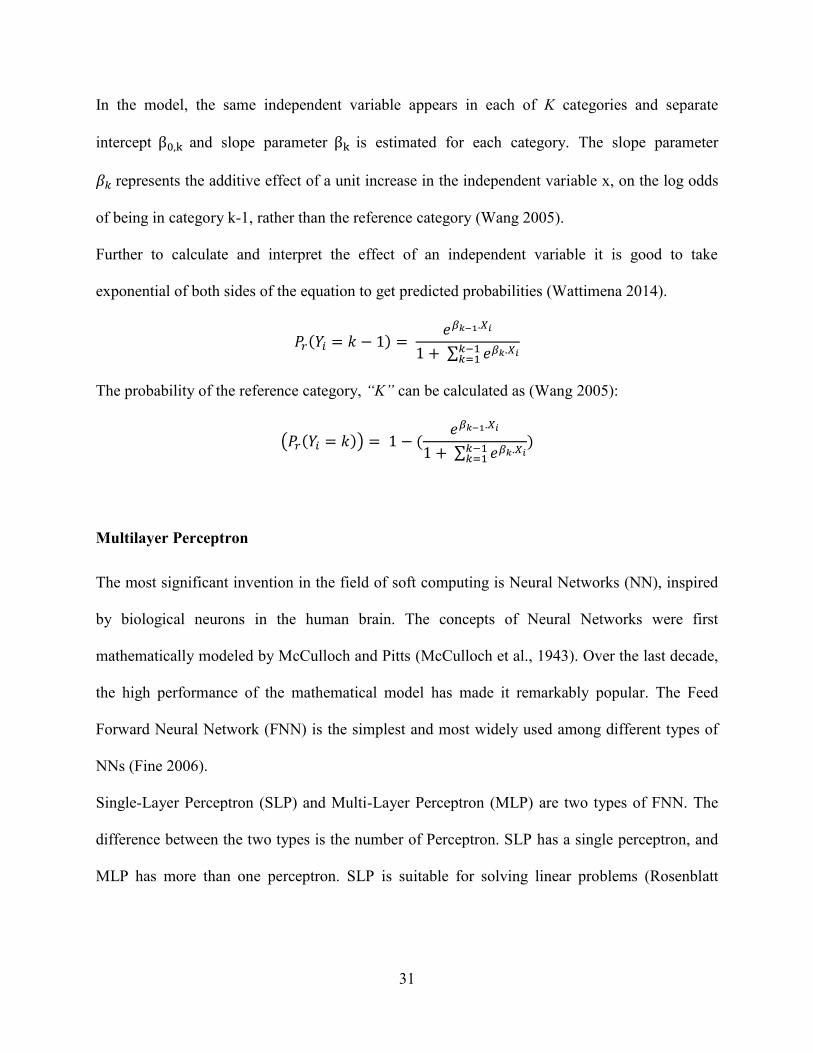
The MLP is a network formed by simple neurons called perceptron. The perceptron calculates a
single output from multiple real-valued inputs by forming combinations of linear relationships
according to input weights and even nonlinear transfer functions. (Mirjalili et al., 2014).
Figure 3 Artificial model of a Neuron. Source: (de Pina et al., 2016).
MLPs are fully connected feed-forward nets with one or more layers of nodes between the input
and the output nodes. Similar, to a biological neural network, MLPs are composed of simple
Page 46
33
interconnected units (the neurons). Each layer is composed of one or more neuron in parallel.
Figure 4 represents an artificial model of a neuron, the McCulloch-Pitts neuron (McCulloch et
al., 1943) Upon receiving a given number of inputs 𝑥𝑖, 𝑖 = 1,2, . . 𝑁, each neuron calculates a
linear combination of the inputs using synaptic weights 𝑤𝑖 to generate the weighted input z; then,
it provides an output y via an activation function 𝑓(𝑧) (de Pina et al., 2016).
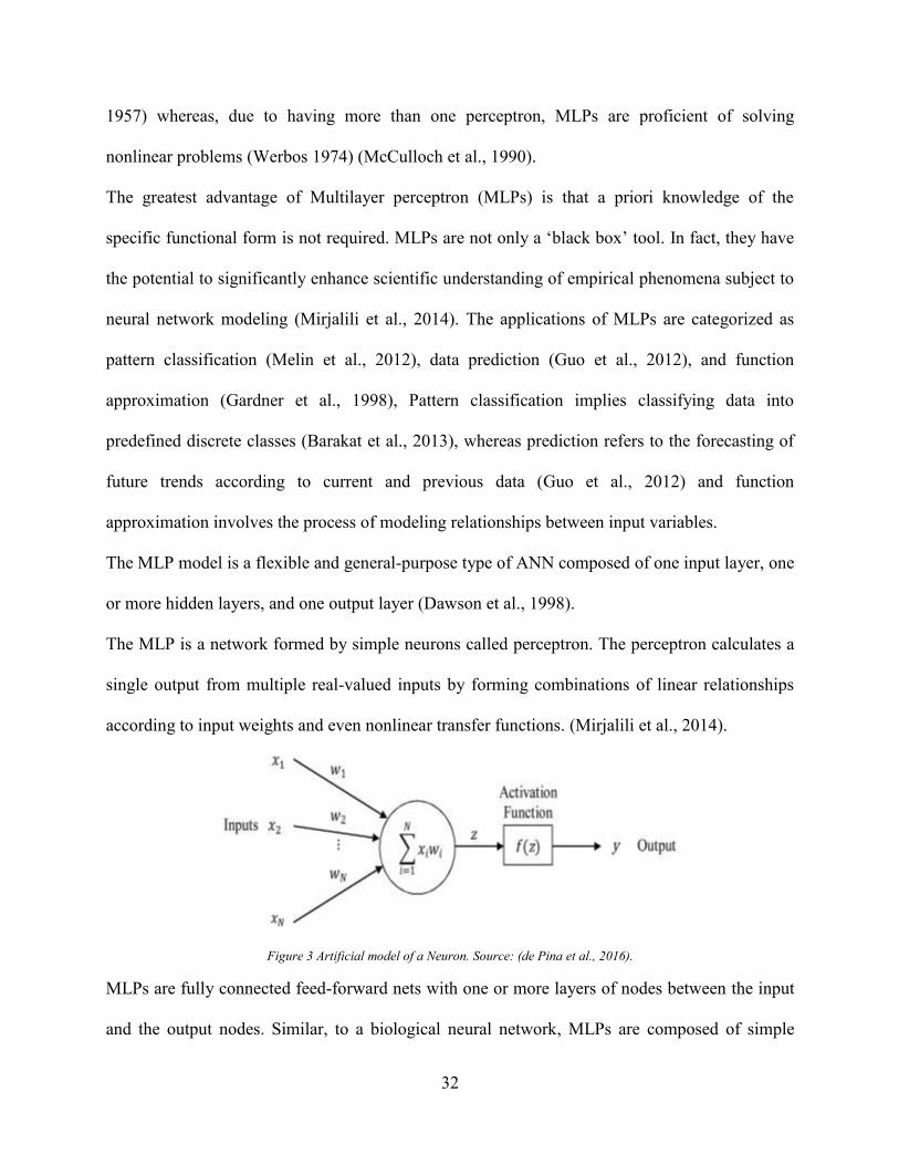
Figure 4 Output Sigmoid Activation Function. Source: (de Pina et al., 2016)
The sigmoid activation function as shown in figure 5 is given by:
𝑦 = 𝑓(𝑧) = 1
1 + 𝑒−𝑧
The activation function should present an increasing monotonic behavior over a determined
range of values for z, with inferior and superior limits. Ideally, it should also be continuous,
smooth and differentiable on all points (de Pina et al., 2016). In this research, we implemented a
sigmoid function, which is the most common type of activation function.
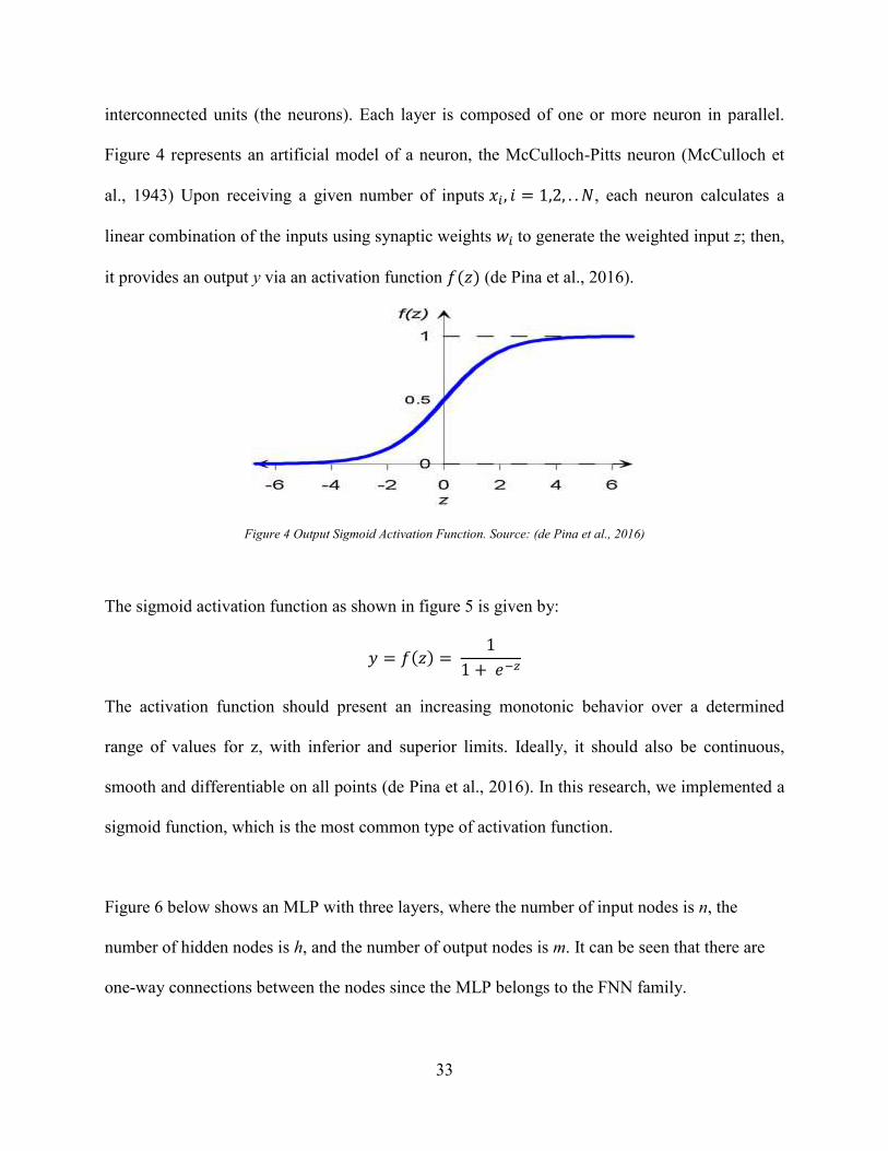
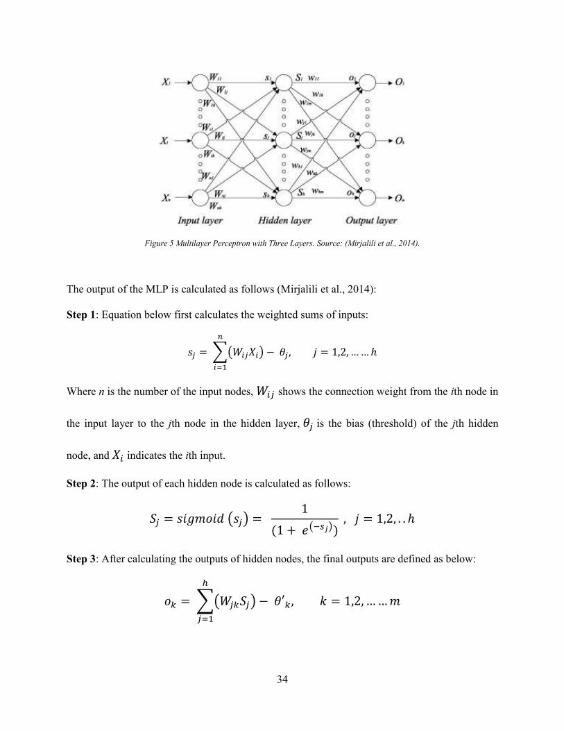
Figure 6 below shows an MLP with three layers, where the number of input nodes is n, the
number of hidden nodes is h, and the number of output nodes is m. It can be seen that there are
one-way connections between the nodes since the MLP belongs to the FNN family.
Page 47
34
Figure 5 Multilayer Perceptron with Three Layers. Source: (Mirjalili et al., 2014).
The output of the MLP is calculated as follows (Mirjalili et al., 2014):
Step 1: Equation below first calculates the weighted sums of inputs:
𝑠𝑗 = ∑(𝑊𝑖𝑗𝑋𝑖) − 𝜃𝑗 , 𝑗 = 1,2, … … ℎ
𝑛
𝑖=1
Where n is the number of the input nodes, 𝑊𝑖𝑗 shows the connection weight from the ith node in
the input layer to the jth node in the hidden layer, 𝜃𝑗 is the bias (threshold) of the jth hidden
node, and 𝑋𝑖 indicates the ith input.
Step 2: The output of each hidden node is calculated as follows:
𝑆𝑗 = 𝑠𝑖𝑔𝑚𝑜𝑖𝑑 (𝑠𝑗) = 1
(1 + 𝑒(−𝑠𝑗)) , 𝑗 = 1,2, . . ℎ
Step 3: After calculating the outputs of hidden nodes, the final outputs are defined as below:
𝑜𝑘 = ∑(𝑊𝑗𝑘𝑆𝑗) − 𝜃′𝑘, 𝑘 = 1,2, … … 𝑚
ℎ
𝑗=1
Page 48
35
𝑂𝑘 = 𝑠𝑖𝑔𝑚𝑜𝑖𝑑 (𝑜𝑘) = 1
(1 + 𝑒(−𝑜𝑘)) , 𝑘 = 1,2, . . 𝑚
Where, 𝑊𝑗𝑘 is the connection weight from the jth hidden node to the kth output node, and 𝜃′𝑘 is
the bias (threshold) of the kth output node.
The most important parts of MLPs are the connection weights and biases. As may be seen in the
above equations, the weights and biases define the final values of output. Training an MLP
involves finding optimum values for weights and biases to achieve desirable outputs from certain
given inputs (Mirjalili et al., 2014).
Back-propagation Algorithm
In our thesis, we used back propagation algorithm to train the Multilayer perceptron model.
The MLP learning algorithm involves a forward-propagating step followed by a backward-
propagating step. The pseudo code for back propagation learning algorithm in the MLP is given
below:
Pseudo code for Back propagation learning algorithm in the MLP (Lek and Park, 2008):
1. Randomize the weights w to small random values.
2. Select an instance t, a pair of input and output patterns, from the training set.
3. Apply the network input vector to the network.
4. Calculate the network output vector z.
5. Calculate the errors for each of the outputs k, the difference (𝛿) between the desired
output and the network output.
6. Calculate the necessary updates for weights ∆𝒘 in a way that minimizes this error.
7. Add up the calculated weights’ updates ∆𝒘 to the accumulated total updates ∆𝒘.
Page 49
36
8. Repeat steps 2–7 for several instances comprising an epoch.
9. Adjust the weights w of the network by the updates ∆𝒘.
10. Repeat steps 2–9 until all instances in the training set are processed. This constitutes one-
iteration.
11. Repeat the iteration of steps 2–10 until the error for the entire system (error 𝛿 defined
above or the error on cross-validation set) is acceptably low, or the predefined number of
iterations is reached.
Forward propagating step
In forward-propagation, the input is fed to the input layer(s), and input propagates and undergoes
the calculations of activation levels and further propagates forward through hidden layer till the
output layer(s). In every successive layer, each neuron sums its inputs and then applies a transfer
function to compute its output. The final answer is the estimate of target value produced by the
output layer of the network (Lek and Park 2008).
Backward-propagating step
In this step, the comparison of the network’s output to the target value is initiated, and the
difference (or error 𝛿) is calculated. The error parameter is used during the weight-correction
procedure. Consider the output layer is designed by k, then error value is given by:
𝛿𝑘 = (𝑡𝑘 − 𝑥𝑘)𝑓′(𝑎𝑘)
Where, 𝑡𝑘 is the target value of unit k, 𝑥𝑘 is the output value for unit k, 𝑓′ is the derivative of the
sigmoid function, 𝑎𝑘 is the weighted sum of input to k, and the quantity (𝑡𝑘 − 𝑥𝑘) reflects the
amount of error. When the sum 𝑎𝑘 is near the rapid rise in the sigmoid curve, the derivative of
Page 50
37
the sigmoid function forces a stronger correction.
The error value for the hidden layer (j), is computed as:
𝛿𝑗 = [∑ 𝛿𝑘𝑤𝑘𝑗𝑘
] 𝑓′(𝑎𝑗)
The connection weight alteration for processing unit is done by using the 𝛿 values of the unit.
Every single weight is adjusted by considering the 𝛿 value of the unit that receives input from
that interconnection. The connection weight adjustment is executed as mentioned below (Lek
and Park 2008):
∆𝑤𝑘𝑗 = 𝜂𝛿𝑘𝑥𝑗
The weight 𝒘𝒌𝒋 alteration, which pass to unit k from unit j, depends on three factors: 𝜹𝒌 (error
value of the target unit) 𝒙𝒋 (output value for the originating unit) and 𝜼 learning rate which is
chosen by user commonly between 0 and 1. 𝜼 represents the learning rate of the network.
Training the network (Lek and Park, 2008)
In back propagation, the error surface of the gradient vector is calculated. This vector points
along the line of steepest descent from the current point, so it is known that if moved along it a
"short" distance, we will decrease the error (Ayodele, 2010). The backpropagation algorithm
executes gradient descent on the error surface by adjusting each weight. The adjustment in
weight is made in proportion to the gradient of the surface at its location. As can be seen in
figure 7 preferably, a global minimum (lowest error value possible) is most desirable but
sometimes gradient descent leads to achieve local minima as a result of the network getting stuck
in a depression in the error surface. These local minima correspond to a partial solution for the
network in response to the training data. A network can be pulled out of local minimum by
Page 51
38
changing the learning parameter, the number of hidden units and momentum term (𝛼) in the
algorithm. The momentum term improves movement in a fixed direction, the algorithm "picks up
speed" if several steps are taken in the same direction which sometimes provides it the ability to
escape local minimum, and also to move rapidly over flat spots and plateaus. The momentum
term is chosen generally between 0 and 1. Taking into account the momentum term (𝛼), the
formula of modifications of weights at epoch t+1 are given by (Lek and Park, 2008):
Δ𝑤𝑘𝑗 (𝑡 + 1) = 𝜂𝛿𝑘𝑥𝑘 + 𝛼Δ𝑤𝑘𝑗 (𝑡)
The learning rate 𝜂 and the momentum term 𝛼 play a vital role in the learning process of Back
propagation network. Efficient selection of the values of these parameters is important to avoid
the network getting into oscillation and getting stuck in local minimum.
Figure 6 Error Surface as Function of a Weight Showing Gradient and Local and Global Minima. Source: (Lek and Park 2008)
Decision trees (ID3 & C4.5)
Decision trees are one of the prominent methods in supervised learning. The trees partition a data
set into groups as similar as possible in terms of the variable to be predicted. It takes a set of
classified data as input and outputs a tree that resembles an alignment diagram where each end
node (leaf) is a decision (a class), and each non-final node (internal) represents a test. Each leaf
Page 52
39
represents the decision of belonging to a class of data verifying all tests path from the root to the
leaf (Hssina et al., 2014). Instances are classified starting at the root node and sorted based on
their feature values. (Kotsiantis et al., 2007).
J. Ross Quinlan originally developed ID3 (Iterative DiChaudomiser 3) (Quinlan, 1986) at the
University of Sydney. The ID3 algorithm builds a tree based on the information (information
gain) obtained from the training instances and then uses the same to classify the test data. ID3
algorithm uses nominal attributes for classification with no missing values (Quinlan, 1986).
The feature that best divides the training data would be the root node of the tree. There are
numerous methods for finding the feature that best divides the training data such as information
gain (Hunt et al., 1966) and Gini index (Breiman et al., 1984) (Kotsiantis et al., 2007).
Decision trees have been used as classifiers for numerous real-world domains, some of which are
mentioned and used as examples by Quinlan; e.g., labor negotiations, hypothyroid diagnosis,
soybean disease diagnosis, and credit approval (Quinlan, 1993).
Information Theory (Hssina et al., 2014):
Entropy is a vital component of Decision tree algorithm. Entropy first defines the amount of
information provided by an event, the higher the probability of an event is low (it is rare), the
more information it provides is great.
Entropy:
If we are given a probability distribution P = (p1, p2,…, pn) and a sample S then the Information
carried by this distribution, also called the entropy of P is giving by:
𝐸 = − ∑ 𝑝𝑖 × 𝑙𝑜𝑔2
𝑛
𝑖=1
𝑝𝑖
Page 53
40
Information gain:
The functions that measure the degree of mixing of classes for all sample and therefore any
position of the tree in construction. It remains to define a function to select the test that must
label the current node. It defines the gain for a test T and a position p
𝐺𝑎𝑖𝑛(𝑝, 𝑇) = 𝐸𝑛𝑡𝑜𝑟𝑜𝑝𝑖𝑒(𝑝) − ∑(𝑝𝑗 × 𝐸𝑛𝑡𝑜𝑟𝑜𝑝𝑖𝑒
𝑛
𝑗=1
(𝑝𝑗))
Where values (𝑝𝑗) is the set of all possible values for attribute T. We can use this measure to
rank attributes and build the decision tree where at each node is located the attribute with the
highest information gain among the attributes not yet considered in the path from the root.
C4.5 Decision Tree
There were few limitations of the ID3 algorithm and in 1993, Ross Quinlan proposed C4.5 to
overcome those limitations. C4.5 algorithm acts similar to ID3 but improves a few of ID3
behaviors (Hssina et al., 2014):
Possibility to use continuous data.
Using unknown (missing) values
Ability to use attributes with different weights.
Pruning the tree after being created.
A tree is constructed by considering the top-down approach. The tree is initialized with
construction at the root node first, where each attribute is assessed using a statistical test, to
determine its classification efficiency of the training samples. The best attribute is chosen as the
test at the root node of the tree. If the attribute is discrete in nature a descendant of the root node
Page 54
41
is created for each possible value of this attribute. If the attribute is continuous in nature a
descendant of the root node is created for each possible discretized interval of this attribute.
In the next step, the training samples are sorted to the suitable descendant node. Further, the
process is repeated using the training samples related with each descendant node to choose the
best attribute specific at that point in the tree, for testing. This forms a greedy search (problem-
solving heuristic of making the locally optimal choice at each stage with the hope of finding a
global optimum) for a decision tree. During this process, the algorithm propagates in forward
direction, i.e., the algorithm never backpedals to reconsider earlier node choices. A node can be
introduced to the tree only when there are a sufficient number of samples left from sorting. After
the complete tree is constructed, in C4.5 tree pruning (depth/size reduction of decision trees by
eliminating parts that provide little information to classify instances) is usually carried out to
avoid data over-fitting (Setsirichok et al., 2012). J48 is an implementation of the C4.5 algorithm
in the Weka data-mining tool.
Statistical test:
Alike ID3 the statistical test used in C4.5 also employs an entropy-based measure for allocating
an attribute to each node in the tree. Like ID3 the data is sorted at every node of the tree to
determine the best splitting attribute. The difference is C4.5 uses gain ratio impurity method to
evaluate the splitting attribute (Quinlan, 1993). At every node, C4.5 selects data attribute which
best splits data into subsets rich in one class or the other. The selection criterion is the
normalized information-gain (difference in entropy) that results from choosing an attribute for
splitting the data. The attribute with the highest normalized information gain is chosen to make
the decision (Quinlan, 1993) (Hssina et al., 2014).
Page 55
42
The information gain ratio is given by:
𝐺𝑎𝑖𝑛𝑅𝑎𝑡𝑖𝑜(𝑝, 𝑇) = 𝐺𝑎𝑖𝑛 (𝑝, 𝑇)
𝑆𝑝𝑙𝑖𝑡𝐼𝑛𝑓𝑜(𝑝, 𝑇)
Where:
𝐺𝑎𝑖𝑛(𝑝, 𝑇) = 𝐸𝑛𝑡𝑜𝑟𝑜𝑝𝑖𝑒(𝑝) − ∑(𝑝𝑗 × 𝐸𝑛𝑡𝑜𝑟𝑜𝑝𝑖𝑒
𝑛
𝑗=1
(𝑝𝑗))
𝑆𝑝𝑙𝑖𝑡𝐼𝑛𝑓𝑜(𝑝, 𝑡𝑒𝑠𝑡) = − ∑ 𝑃′
𝑛
𝑗=1
(𝑗
𝑝) × log(𝑃′ (
𝑗
𝑝))
𝑃′ (𝑗
𝑝) is the proportion of elements present at the position p, taking the value of j-th test.
Pseudocode C4.5 (Kotsiantis et al., 2007):
1. If ({All the samples in the list belong to the same class}
Then {create a leaf node to choose that class})
If ({None of the features provide any information gain}
Then {create a decision node higher up the tree using the expected value of the
class})
If ({Instance of previously unseen class encountered}
Then {create a decision node higher up the tree using the expected value})
2. Check for above cases
3. For each attribute a, evaluate information gain ratio (normalized) from splitting on a.
4. Let a_best be the attribute with the highest normalized information gain.
5. Create a decision node that splits on a_best.
6. Recurse on the sublists obtained by splitting on a_best, and add those nodes as children
of the node.
Page 56
43
3.3 Method Improvement (Ensemble Learning)
Ensemble learning techniques train multiple classifiers instead of just one classifier to solve the
same learning problem (Zhou, 2012). Many researchers have investigated the technique of
combining the predictions of multiple classifiers to produce a single classifier. The resulting
classifier is generally more accurate than any of the individual classifiers making up the
ensemble (Opitz et al., 1999).
An ensemble contains a number of classifiers called base learners. Base learners are usually
generated from training data by a base learning algorithm which can be decision tree, neural
network or other kinds of learning algorithms. Ensemble methods construct a set of learners and
combine them. Base learners are also called as weak learners because the generalization power
of an ensemble is usually stronger than base learner and hence provide improved prediction
accuracy. Ensemble methods using the same base learner for learning are called homogenous
ensembles (Zhou 2012). Figure 8 represents generalized ensemble architecture.
Figure 7. General Ensemble Architecture. Source: (Zhou 2012).
The individual decisions of base learners in an ensemble are combined in some way (usually
either by averaging or weighted/unweighted voting) to classify new examples. As an ensemble
can be trained and used for classification, these learning algorithms lie under the category of
supervised learning (Dietterich, 2000). The empirical analysis presented by Hanson and Salmon
Page 57
44
in 1990, showed that prediction accuracy of an ensemble of classifiers is often more accurate
than individual best single classifier. Figure 9 illustrates the simplified version of observation
obtained by marking noise level vs. error (Hansen et al., 1990).
Figure 8. Classifier Performance Marked on Noise Level vs. Error. Source: (Zhou 2012).
According to (Hansen et al., 1990), in order for an ensemble to be more accurate than its base
learners, the important condition is that the base learners/classifiers should be accurate (error rate
on new input values should be better than guessing) and diverse (different error rate on new input
values).
Ensembles learning for weak learners were extensively studied in the machine learning
community. Extensive work by the researchers in this domain led to the birth of two popular
methods for creating accurate ensembles, i.e., Bagging (Breiman, 1996) and Boosting (Freund et
al., 1996). In this research, we used ensemble methods like bagging and boosting to improve the
prediction accuracy of best-performing machine learning model for GHG emission by road
transport in Canada.
Page 58
45
Ensemble methods have been used on various occasions, which involved learning techniques and their exploitation. Table 2 shows the
domains which have been benefitted by using ensemble techniques:
Table 2. Domains Benefitted By Ensemble Techniques
Domains Paper Title Authors
Computer vision (Object
detection, recognition, and
tracking)
Robust real-time face detection.
Pose invariant face recognition. In Automatic Face and
Gesture Recognition.
Viola & Jones (2004), Huang et al. (2000).
Computer security (intrusion
detection, Malware detection,
etc.)
Fusion of multiple classifiers for intrusion
detection in computer networks.
Data mining methods for detection of new
malicious executables.
Giacinto et al. (2003), Schultz et al. (2001).
Computer aided medical
diagnosis.
Medical diagnosis with C4. 5 rule preceded by
artificial neural network ensemble.
An ensemble based data fusion approach for early
diagnosis of Alzheimer’s disease
Zhou & Jiang (2003), Polikar et al. (2008).
Credit card fraud detection
Distributed data mining in credit card fraud
detection.
Credit card fraud detection: A fusion approach
using Dempster–Shafer theory and Bayesian
learning
Chan et al., (1999), Panigrahi et al.,(2009).
Bankruptcy detection
Neural network ensemble strategies for financial decision
applications West et al., (2005)
Species distribution Forecasting Ensemble forecasting of species distributions. Araújo & New (2007)
Weather forecasting
An ensemble of neural networks for weather forecasting Maqsood et al. (2004)
Aircraft engine fault diagnosis
Jet engine gas path fault diagnosis using dynamic
fusion of multiple classifiers
Diagnostic information fusion: requirements flow
down and interface issues.
Yan & Xue (2008), Goebel et al. (2000)
Artist classification
Aggregate features and AdaBoost for music classification. Bergstra et al. (2006)
Page 59
46
3.3.1 Bagging
It is most commonly known as bootstrap aggregation. The two important elements of Bagging
algorithm are bootstrap and aggregation (Breiman, 1996).
Table 3 shows Pseudo Code for Bagging algorithm. Bagging deploys bootstrap sampling to
obtain the data subsets for training the base learners. Consider a training data set containing m
number of training examples, sampling with replacement will generate a sample of m training
examples. Some original examples may appear more than once, while some original examples
are not present in the sample. Repeating the process T times, T samples of m training examples
are obtained. Then, from each sample, a base-learner/classifier can be trained by applying the
base-learning/classifier algorithm (Zhou, 2012) (Breiman, 1996).
Pseudo code:
Table 3. Bagging Pseudo Code. Source: (King et al., 2014)
Page 60
47
Each bootstrap replicates contain, on an average 63.2% of the original training set, with multiple
repetitions of example from the training set. Additionally, bagging reduces variance (Breiman,
1996) (Dietterich, 2000).
Bagging uses voting for classification and averaging for regression to aggregate the outputs of
the base learners (Zhou, 2012). For example in a classification problem, the algorithm inputs an
instance to its base learners and collects their outputs. Voting the labels follows this process, and
finally, the algorithm chooses the winner label as a prediction. Bagging algorithm is functional
with binary as well as multi class problems (Zhou, 2012).
3.3.2 Boosting
Boosting (Freund et al., 1996) incorporates a family of methods. This ensemble method produces
a series of classifiers. Based on the performance of the previous classifier(s) in series, the
training set used for each member classifier of the series is chosen. According to the logic of
Boosting algorithm, it gives less emphasis to correctly classified examples by the classifier in
series and give more emphasis on previously misclassified examples by a classifier in series, by
choosing them more frequently compared to correctly predicted examples. In general, the
Boosting algorithm tries to generate new classifiers that are better able to predict examples for
which the current ensemble’s performance is poor (Opitz et al., 1999).
The most popular boosting procedure is AdaBoost-M1(Adaptive Boosting). This procedure
allows continuing adding weak learners until some desired low training error is achieved.
Page 61
48
Adaptive Boosting Algorithm M1 (Freund et al., 1996):
Consider the input to the boosting algorithm takes a training set of m examples.
𝑆 = ((𝑥1, 𝑦1), . . , (𝑥𝑚, 𝑦𝑚)) Where, 𝑥𝑖 is an instance drawn from some space X and represented
in some manner (typically, a vector of attribute values) and, 𝑦𝑖 ∈ 𝑌 is the class label associated
with 𝑥𝑖.
The boosting algorithm invokes Weak Learner (base algorithm) repeatedly in a series of rounds.
On round t, the algorithm provides weak learners with a distribution (𝐷𝑡) over the training set S.
Following the reception of distribution the weak learners computes a classifier or hypothesis
ℎ𝑡 ∶ 𝑋 → 𝑌 which should correctly classify a fraction of the training set that has large probability
with respect to (𝐷𝑡).
The weak learner’s goal is to find hypothesis ℎ𝑡, which minimizes the training error.
𝜖𝑡 = 𝑃𝑟𝑖 ~ 𝐷𝑡 [ℎ𝑡 (𝑥𝑖) ≠ 𝑦𝑖]
This error is measured with respect to the distribution (𝐷𝑡) that was provided to the weak
learner. This process continues for T rounds, and at last the boosting algorithm combines the
weak hypotheses ℎ1, … . ℎ𝑇 into a single final hypothesis (ℎ𝑓𝑖𝑛)
Pseudo code (Freund et al., 1996):
Input: Sequence of m examples ((𝑥1, 𝑦1), . . , (𝑥𝑚, 𝑦𝑚)) with labels 𝑦𝑖 ∈ 𝑌 = {1, … , 𝐾}
Weak learning algorithm and integer T specifying number of iterations
Page 62
49
Initialize: 𝐷1(𝑖) =1
𝑚 for all i.
Do for t = 1,2,.., T:
1. Call Weak learning algorithm, providing it with distribution (𝐷𝑡).
2. Get back a hypothesis ℎ𝑡 ∶ 𝑋 → 𝑌.
3. Calculate the error of ℎ𝑡
ℎ𝑡: 𝜖𝑡 = ∑ 𝐷𝑡(𝑖)𝑖:ℎ𝑡(𝑥𝑖)≠ 𝑦𝑖.
If 휀𝑡 > 0.5, then set T = t-1 and abort loop.
4. Set 𝛽𝑡 = 𝜖𝑡
(1− 𝜖𝑡) .
5. Update distribution (𝐷𝑡):
𝐷𝑡+1(𝑖) = 𝐷𝑡(𝑖)
𝑍𝑡 × 𝛽𝑡 (if ℎ𝑡(𝑥𝑖) = 𝑦𝑖) or
𝐷𝑡+1(𝑖) = 𝐷𝑡(𝑖)
𝑍𝑡 × 1 (otherwise)
Where, 𝑍𝑡is a normalization constant (chosen so that 𝐷𝑡+1 will be a distribution).
Output the final hypothesis:
𝒉𝒇𝒊𝒏(𝒙) = 𝒂𝒗𝒆𝒓𝒂𝒈𝒆 𝒎𝒂𝒙𝒚∈𝒀 ∑ 𝑙𝑜𝑔1𝛽𝑡𝑡:ℎ𝑡(𝑥)= 𝑦
.
AdaBoost.M1 uses a simple rule for calculating Distribution and final hypothesis as shown
below.
Page 63
50
Distribution (𝑫𝒕) Calculation (Freund et al., 1996):
The initial distribution 𝐷𝑖 is uniform over S so, 𝐷1(𝑖) =1
𝑚 for all i. To compute distribution
𝐷𝑡+1 from 𝐷𝑡 and last week hypothesis ℎ𝑡, we multiply the weight of example i by some number
𝛽𝑡 ∈ [0,1] if ℎ𝑡 classifies 𝑥𝑖 correctly, or else the weight is left unchanged. The weights are
then renormalized by dividing by the normalization constant 𝑍𝑡 effectively, “easy” examples that
are correctly classified by many of the previous weak hypotheses get lower weight, and “hard”
examples which tend often to be misclassified get higher weight. AdaBoost focuses the most
weight on the examples, which seem to be hardest for Weak Learners.
Final hypothesis Calculation (𝒉𝒇𝒊𝒏) (Freund et al., 1996):
The number 𝛽𝑡 is calculated as a function of 𝜖𝑡. The final hypothesis (𝒉𝒇𝒊𝒏) is a weighted vote
(i.e., a weighted linear threshold) of the weak hypotheses. That is, for a given instance x, (𝒉𝒇𝒊𝒏)
outputs the label y that maximizes the sum of the weights of the weak hypotheses predicting that
label. The weight of hypothesis ℎ𝑡 is given by log(1
𝛽𝑡) so that greater weight is given to
hypotheses with lower error.
In chapter 4 we will be adapting the data mining techniques mentioned in chapter 3 to perform
predictive modeling of GHG emissions caused by road transportation (passenger & freight).
Furthermore using the best performing model, a scenario analysis will be conducted to
demonstrate the model’s applicability in the context of Canadian road transport GHG emissions
predictions and component distribution (emissions share of different road vehicle) all the way
through the year 2030.
Page 64
51
Chapter 4
Research Methodology
Our research methodology is divided into 3 different phases:
Phase 1: Study of GHG Emissions Landscape of Canada
Phase 2: Supervised learning model development (Regression & Classification) and applications
for emissions prediction
Feature Selection
Multiple Linear Regression
Logistic regression
Decision tree (C4.5)
Multilayer Perceptron (ANN)
Bagging
Boosting
Phase 3: Canada GHG emissions scenario analysis
Business as usual scenario
Minimum mitigation scenario (M1)
Maximum mitigation scenario (M2)
Page 65
52
Figure 9 Flowchart of Research steps
Page 66
53
Phase 1: GHG Emissions Landscape of Canada
4.1 GHG emissions in Canada
According to (Government of Canada, et al., 2017) as of 2015, Canada’s total greenhouse house
gas GHG emissions was 722 (MtCo2Eq.) with respect to emission breakdown by economic
sector. Figure 10 shows Canada's national greenhouse gas emissions in mega tonnes of carbon
dioxide equivalent from 1990 to 2015. Source: Environment and Climate Change Canada (2017)
National Inventory Report 1990–2015
Page 67
54
According to (Government of Canada, et al., 2017) Canada's emissions growth between 1990
and 2015 was mainly caused by increased emissions from mining and upstream oil and gas
611 604 621 623
644 661
682 697 704 717 738 728 730
749 751 738 729 750
729 689 701 707 716 729 727 722
0
100
200
300
400
500
600
700
800
19
90
19
91
19
92
19
93
19
94
19
95
19
96
19
97
19
98
19
99
20
00
20
01
20
02
20
03
20
04
20
05
20
06
20
07
20
08
20
09
20
10
20
11
20
12
20
13
20
14
20
15
Total greenhouse gas emissions over the years (megatones of carbon
dioxide equivalent)
Figure 10 Total GHG Emissions over the Years (MtCo2eq.)
Page 68
55
production as well as transport. Emission reductions from 2005 to 2015 were results of reduced
emissions from public electricity and heat production utilities. The GHG emission given above
includes emissions from seven GHG gases namely: carbon dioxide, methane, nitrous oxide,
sulfur hexafluoride, perfluorocarbons, hydrofluorocarbons, and nitrogen trifluoride.
4.1.1 GHG analysis in Canada
GHG Emission in Canada are categorized as per the below two sectors (Government of Canada,
Canada's GHG Inventory 2017):
Intergovernmental Panel on climate change (IPCC) sector:
GHG emissions are categorized into the following five sectors as per IPCC: Energy, Industrial
Processes and Product Use, Agriculture, Waste and Land Use, Land-Use Change and Forestry.
In IPCC a rounding protocol has been developed for the emission and removal estimates
presented by activity sectors defined by the Intergovernmental Panel on Climate Change to
reflect their uncertainty levels. In rounding Protocols, estimates have been rounded to the nearest
1Mt and 0.1Mt for National-level estimates and provincial/territorial-level estimates. As a result
of these procedures, individual values in the emission tables may not add up to the subtotals and
overall totals (Government of Canada, Canada's GHG Inventory 2017).
Economic Sector:
To analyze economic trends, GHG emissions are categorized to the economic sector from which
they originate. Canada’s emission is categorized by following economic sector:
Oil and Gas, Electricity, Transportation, Heavy Industry, Buildings, Agriculture, Waste, and
Others. The IPCC rounding protocol does not apply to estimates presented by Canadian
Economic Sectors.
Page 69
56
Figure 11. GHG Emission by Canadian Economic Sector
4.1.2 Greenhouse gas emissions by Canadian Economic Sector
Figure 11 shows GHG emissions increase of 82 MtCo2Eq. and 51 MtCo2Eq between 1990 and
2015 was mostly due to rise in emissions from the oil & gas and the transportation sector. These
increases in emissions from the oil & gas and the transportation sector were offset by a
16 MtCo2Eq. decrease in emissions in the electricity sector and a 22 MtCo2Eq. decrease in
emissions from heavy industry (Government of Canada, Canada's GHG Inventory 2017). Data
Source: Environment and Climate Change Canada (2017) National Inventory Report 1990–2015.
1990, 107.7 2015, 189.5
1990, 121.8
2015, 173 1990, 73.5
2015, 85.6
1990, 94.5
2015, 78.7 1990, 96.6
2015, 74.6 1990, 60.1
2015, 72.8
1990, 56.9
2015, 47.6
0
100
200
300
400
500
600
700
800
19
90
19
91
19
92
19
93
19
94
19
95
19
96
19
97
19
98
19
99
20
00
20
01
20
02
20
03
20
04
20
05
20
06
20
07
20
08
20
09
20
10
20
11
20
12
20
13
20
14
20
15
Canada GHG Emission in years (megatonnes of carbon dioxide equivalent)
Waste and others (megatonnes ofcarbon dioxide equivalent)
Agriculture (megatonnes of carbondioxide equivalent)
Heavy industry (megatonnes of carbondioxide equivalent)
Electricity (megatonnes of carbondioxide equivalent)
Buildings (megatonnes of carbondioxide equivalent)
Transportation (megatonnes of carbondioxide equivalent)
Oil and gas (megatonnes of carbondioxide equivalent)
Page 70
57
Figure 12. GHG Emission by Canadian Economic Sector in 2015
Figure 12 shows that in 2015, total greenhouse gas (GHG) emissions in Canada were
722 (MtCo2eq). Oil & gas sector was the biggest contributor to GHG emissions emitting 26% of
total emissions in 2015, followed by the transportation sector, which emitted 24%. The other
Canadian economic sectors (i.e., buildings, electricity, heavy industry, agriculture, and waste and
others), each accounted for 12% 11% 10% 10% and 7% respectively of total GHG emissions in
Canada.
Oil and gas (megatonnes of carbon
dioxide equivalent), 189.5, 26%
Transportation (megatonnes of carbon
dioxide equivalent), 173, 24%
Buildings (megatonnes of carbon dioxide
equivalent), 85.6, 12%
Electricity (megatonnes of carbon dioxide
equivalent), 78.7, 11%
Heavy industry (megatonnes of carbon
dioxide equivalent), 74.6, 10%
Agriculture (megatonnes of carbon
dioxide equivalent), 72.8, 10%
Waste and others (megatonnes of carbon
dioxide equivalent), 47.6, 7%
GHG Emission 2015- Economic Sector
Page 71
58
4.1.3 Provincial GHG Analysis in Canada
89 80.1
181.3
166.2
20.8
45.2
75
175.3
274.1
51.9 60.9
0
50
100
150
200
250
300
1990 2005 2010 2011 2012 2013 2014 2015
Provincial GHG Emissions over the years
Newfoundland & Labrador
Prince Edward Island
Nova Scotia
New Brunswik
Quebec
Ontario
Manitoba
Saskatchewan
Alberta
British Columbia
Yukon
Northwest Territories
Nunavut
Page 72
59
Figure 13 shows Canadian Provincial GHG Emissions over the Years. Each province has
different Emission levels. According to (Government of Canada, Environment and Climate
Change Canada 2017), this significant difference depends on population, energy sources and
economic base. The provincial economies, which are service-based economies had lower
emission levels whereas the economies based on natural resource extraction usually had higher
emission levels in comparison. The provinces like Ontario, which bank on fossil fuels for their
power requirement (electricity generation) had greater emissions share compared to the
provinces relying on renewable sources to meet their energy needs like Quebec. The data for the
figure 13 is given in Appendix A.
As can be seen in figure 13, in 1990, Alberta's emissions exceeded Ontario by 56% since 1990,
largely due to the increase in the oil and gas industry for export markets. And because of large
manufacturing industry, Ontario's GHG emissions were higher than those from the other
provinces. Between 1990 and 2015, Ontario's emissions reduced mostly because of the
termination of coal-fired electricity generation plants (Government of Canada, Environment and
Climate Change Canada 2017). After adopting Climate Action plan in the year 2008, a steady
decrease in BC’s emission trend from 63.9 (Mt Co2 eq.) in 2005 to 60.9 (Mt Co2 eq.) in 2015 is
observed as a result of carbon pricing.
Pareto analysis
Figure 13. Provincial GHG Emissions over the Years
Page 73
60
Joseph Juran named this technique after an Italian economist Vilfredo Pareto, as he observed that
80% of the effects resulted due to the 20% of the causes (Juran, 1992). A Pareto diagram is a
simple histogram of the data entries sorted from largest to lowest frequency, and a cumulative
frequency curve is obtained. Pareto analysis is widely used as a statistical tool by employees
undertaking improvement projects in numerous organizations to isolate the most impactful
problems from a relatively larger number of problems. As a result, the problems, which are most
significant, stand out and provide opportunities for improvements.
In the present study, we employed Pareto analysis to identify the provinces, which are major
contributors of GHG emissions within Canada, i.e., “vital few” (Canadian provinces) from
“Trivial many” (Canada).
To determine contributors of GHG emission from Canadian provinces, we performed Pareto
analysis on the Provincial GHG emission data (Appendix B) of 2015. This data was categorized
by economic sector.
Page 74
61
37.97
61.00
72.10
82.49
90.93 93.81 96.05 98.00 99.43 99.68 99.88 99.96 100.00
0.00
10.00
20.00
30.00
40.00
50.00
60.00
70.00
80.00
90.00
100.00
0
50
100
150
200
250
300
Pareto Analysis GHG Emissions by provinces in 2015
Frequency Percentage
Figure 14. Pareto Analysis of GHG Emissions by Provinces in 2015
Page 75
62
Figure 15. Major GHG Emission Provinces in 2015 Distribution by Economic Sector
The result of Pareto analysis as shown in Figure 14 shows that Alberta, Ontario, Quebec, and
Saskatchewan are the major contributors of GHG emissions in Canada. In the year 2015,
Canadian provinces of Alberta, Ontario, Quebec, and Saskatchewan were the major contributors
of GHG emissions in Canada. Combined all together these four Canadian provinces contributed
82.49% (595.4 megatons (Mt) of carbon dioxide equivalent (CO2 eq)) in overall GHG emissions
(722 megatons (Mt) of carbon dioxide equivalent (CO2 eq).
4.1.4 Major GHG Emitting Provinces (GHG Emission Distribution by Economic Sector)
0
20
40
60
80
100
120
140
Oil
& G
as
Ele
ctri
city
Tra
nsp
ort
atio
n
Hea
vy
Ind
ust
ry
Bu
ild
ings
Agr
icu
ltu
re
Was
te
Co
al P
rod
uct
ion
Lig
ht
Man
ufa
ctu
rin
g,C
on
stru
ctio
n &
Fo
rest
Res
ou
rces
Major GHG Emission Provinces in 2015 by Economic Sector
Alberta Ontario Quebec Saskat British Columbia
Page 76
63
Figure 15 shows the GHG distribution of top five major GHG emitting provinces of Canada by
economic sector; we considered the province of British Columbia since British Columbia along
with top four GHG emitting provinces contributed over 90% in overall GHG emissions in the
year 2015 (Appendix C). We further studied the distribution of GHG emissions from each
province with respect to economic sectors.
Figure 16. Top Five GHG Emitting Canadian Provinces of 2015
Page 77
64
Figure 18. Ontario 2015 GHG Emission Distribution by Economic Sector
4.1.5 GHG Distribution of Top Five High Emission Provinces in 2015
Figure 17 shows Alberta’s 2015 GHG Emission Distribution by Economic Sector. In the year
2015, Alberta was the highest contributor of GHG emission (i.e., it contributed 274.1 Mt Co2
eq.). On further analyzing the economic sectors contributing to this number of GHG emissions
within Alberta, it was found that Oil & gas sector is responsible for emitting 49% of the total
GHG emitted by Alberta. Followed by Electricity and Transportation, which contributed 17%
and 11% respectively. Furthermore, within the transportation sector, freight transport contributes
by 7% in Alberta’s GHG emissions, and passenger transport contributes 4%.
Figure 18 shows Ontario’s 2015 GHG Emission Distribution by Economic Sector. In the year
2015, Ontario was the second highest contributor in Canadian GHG emission (i.e., it contributed
166.2 Mt Co2 eq.).
Oil & Gas, 10.3, 6%
Electricity, 5.2, 3%
Heavy Industry, 29.1, 18%
Buildings, 36.8, 22%
Agriculture, 12.3, 8% Waste, 8.6, 5% Coal Production, 0,
0%
Light Manufacturing, Construction & Forest
Resources, 8.9, 6%
Passenger Transport, 35.3,
21%
Freight Transport, 18.7, 11% Transportation
Ontario 2015 GHG Emission by Economic Sector Oil & Gas, 132.3, 49%
Electricity, 46.1, 17%
Heavy Industry, 17, 6%
Buildings, 19.3, 7%
Agriculture, 21.5, 8%
Waste, 2.3, 1%
Coal Production, 0.4, 0%
Light Manufacturing, Construction & Forest
Resources, 2.7, 1%
Passenger Transport, 11.8, 4%
Freight Transport, 19.8, 7%
Transportation 11%
Alberta 2015 GHG Emission by Economic Sector
Figure 17. Alberta 2015 GHG Emission Distribution by Economic Sector
Page 78
65
Figure 19 Quebec 2015 GHG Emission Distribution by Economic Sector
The major economic sectors contributing to this number of GHG emissions within Ontario were
Transportation, Heavy Industry, and Building sector. Transportation sector emits 32% of total
GHG from Ontario followed by Heavy Industry and Building sector, i.e., 18% and 22%
respectively.
Furthermore, within the transportation sector, passenger transport contributes 21%, and freight
transport contributes 11% to Ontario’s GHG emissions.
Figure 19 shows Quebec’s 2015 GHG Emission Distribution by Economic Sector. Quebec was
the third highest contributor in overall Canadian GHG emission (i.e., it contributed 80.1 Mt Co2
eq.). The major economic sectors contributing to this number of GHG emissions within Quebec
were Transportation, Heavy Industry, and Building sector.
Oil & Gas 2.8 4%
Electricity 0.3 0%
Heavy Industry 15.8 20%
Buildings 11.3 14%
Agriculture 9
11% Waste 5.1 7%
Coal Production 0
0%
Light Manufacturing, Construction &
Forest Resources
4.7 6%
Passenger Transport
18.1 23%
Freight Transport
11.5 15%
Transportation
Quebec 2015 GHG Emission by Economic Sector
Page 79
66
Oil & Gas, 13.7, 22%
Electricity, 0.4, 1%
Heavy Industry, 6, 10%
Buildings, 7.3, 12%
Agriculture, 2.9, 5%
Waste, 4.3, 7% Coal Production, 1.7, 3% Light Manufacturing, Construction & Forest
Resources, 2, 3%
Passenger Transport, 10.7, 18%
Freight Transport, 11.7, 19%
Transportation
British Columbia 2015 GHG Emission by Economic Sector
Figure 20. Saskatchewan 2015 GHG Emission Distribution by Economic Sector
Figure 21. British Columbia 2015 GHG Emission Distribution by Economic Sector
Oil & Gas, 24.1, 32%
Electricity, 14.6, 20%
Heavy Industry, 3.2, 4%
Buildings, 3.1, 4%
Agriculture, 17.9, 24%
Waste, 1.1, 2%
Coal Production, 0, 0%
Light Manufacturing, Construction & Forest
Resources, 0.7, 1%
Freight Transport,
5.1, 7%
Passenger Transport,
4.5, 6%
Transportation
Saskatchewan 2015 GHG Emission by Economic Sector
Transportation sector emits 38% of total GHG from Quebec followed by Heavy Industry,
Building sector and Agriculture, i.e., 20%, 14%, and 11% respectively. Furthermore, the
passenger transport within the transportation sector contributes 23%, and freight transport
contributes 15% to Quebec’s GHG emissions.
Figure 20 shows Saskatchewan’s 2015 GHG Emission Distribution by Economic Sector.
Saskatchewan contributed 75 Mt Co2 eq. of GHG emission in the year 2015. The major
economic sectors contributing to this number of GHG emissions within Saskatchewan was Oil &
Gas, Agriculture, and Electricity sector. The Oil & gas sector is responsible for emitting 32% of
the total GHG emitted by Saskatchewan. Followed by Agriculture, Electricity, and
transportation, which contributed 24%, 20%, and 13% respectively.
Furthermore, within the transportation sector, freight transport contributes by 7% in
Saskatchewan’s GHG emissions, and passenger transport contributes 6%.
Figure 21 shows British Columbia’s 2015 GHG Emission Distribution by Economic Sector.
British Columbia contributed 60.9 Mt Co2 eq. of GHG emission in the year 2015.
Page 80
67
The major economic sectors contributing to this number of GHG emissions within British
Columbia were Transportation, Oil & Gas, Building and Heavy Industry sector. Transportation
sector emits 37% of total GHG from British Columbia followed by Oil & Gas, Building and
Heavy Industry, i.e., 22%, 12%, and 10% respectively. Furthermore, the freight transport within
the transportation sector contributes 19%, and passenger transport contributes 18% of British
Columbia’s GHG emissions. In British Columbia, Transportation sector emits 37% of total GHG
from BC followed by Oil & Gas and Building sector, i.e., 22% and 12% respectively.
4.1.6 GHG emission by Transportation Sector
In this thesis, we used the data categorized by IPCC to analyze the GHG emission trend by the
Transportation sector. Concerning the IPCC data, the below graph represents GHG emission by
transportation sector in Canada.
The transportation sector was the second largest source of GHG emission accounting 24% of
total Canadian emission in the year 2014 (Appendix D).
Page 81
68
Figure 22. GHG Emissions over the years in Canada by different modes of Transportation
Figure 22 portrays GHG Emissions over the years in Canada by different modes of
Transportation. Emissions from cars over the years declined whereas emission from light trucks
and Freight trucks almost doubled. Also, the minute decrease has been observed in GHG
1990, 49.31 2014, 36.10
1990, 21.85 2014, 45.92
1990, 8.25
2014, 21.99 1990, 17.82
2014, 36.47
1990, 12.86
2014, 18.61
1990, 6.66
2014, 7.36
1990, 7.85
2014, 5.88
1990, 3.69
2014, 7.67
0.00
20.00
40.00
60.00
80.00
100.00
120.00
140.00
160.00
180.00
200.001
99
0
19
91
19
92
19
93
19
94
19
95
19
96
19
97
19
98
19
99
20
00
20
01
20
02
20
03
20
04
20
05
20
06
20
07
20
08
20
09
20
10
20
11
20
12
20
13
20
14
GHG Emissions over the years in Canada by different modes of Transportation
Off-Road1
Marine
Freight Rail
Passenger Rail
Freight Air
Passenger Air
Inter-City Buses
Urban Transit
School Buses
Motorcycles
Heavy Trucks
Medium Trucks
Light Trucks
Cars
80.91 92.31
47.74
85.08
132.34
185.06
0.00
20.00
40.00
60.00
80.00
100.00
120.00
140.00
160.00
180.00
200.00
1985 1990 1995 2000 2005 2010 2015 2020
Total GHG Emission (Transportation)
PassengerTransportation
Freight Transportation
Off-Road1
Total GHG EmissionsExcluding Electricity (Mt)
Page 82
69
Figure 23. Total GHG Emission by Transportation Sector
Figure 24. Total Transportation GHG Emission by Transportation in 2014
emissions from Marine, Passenger rail, Freight Air and Inter-city Buses.
Figure 23. Represents the trend of GHG emission by broad categories of transportation sector
(Appendix E). It can be seen that GHG emissions from freight transportation are showing an
increasing trend since 2009. In general, compared to emissions from 1990 there has been a
steady increment of 14% in GHG emission from passenger transport whereas, on the other hand,
emission from freight transport increased by 78%.
Passenger Transportation,
92.31, 50%
Freight Transportation,
85.08, 46%
Off-Road1, 7.67, 4%
TOTAL TRANSPORTATION GHG EMISSION BY TRANSPORTATION TYPE IN 2014
Passenger Transportation Freight Transportation Off-Road1
Page 83
70
Figure 25. GHG Emissions Over the years By Road Transportation
According to the recent IPCC data for the year 2014. Passenger Transportation emitted 92.31 Mt
of Co2 eq GHG, i.e., 50% of the total GHG emissions caused by transportation and Freight
Transportation emitted 85.08 Mt of Co2 eq GHG, i.e., 46% in total (Appendix E).
4.1.7 GHG Emission by Road Transport
Over the years from 1990, the contribution of GHG emissions from Transportation sector grew
by 52.72 Mt Co2 eq. (39.8%) By the year 2014 (figure 23). As shown in figure 25. Emission
from cars declined by 26% while emission from light trucks increased by 110%, emission from
Heavy trucks increased by 104% and emission from Medium trucks increased by 161% with
respect to 1990 emissions (Appendix F).
49.31
36.10
21.85
45.92
8.25
21.99
17.82
36.47
0.00
10.00
20.00
30.00
40.00
50.00
60.00
19
90
19
91
19
92
19
93
19
94
19
95
19
96
19
97
19
98
19
99
20
00
20
01
20
02
20
03
20
04
20
05
20
06
20
07
20
08
20
09
20
10
20
11
20
12
20
13
20
14
GHG Emissions Over the years By Road Transportation
Cars Light Trucks Medium Trucks Heavy Trucks
Motorcycles School Buses Urban Transit Inter-City Buses
Page 84
71
Figure 26. GHG Emission Distribution by Road Transport-2014
Figure 26. represents GHG Emission Distribution for 2014 by Road Transport. According to the
latest IPCC GHG emission data for the year 2014 (Appendix F), Trucks (Light, Medium, and
Heavy) emitted 92.91 Mt Co2 eq. i.e., 72% of GHG emissions caused by road transportation
(144.97 Mt c02 eq.).
Within the category of trucks, Light Trucks (trucks, vans and sport utility vehicles) emitted 45.92
Mt co2 eq.; Heavy trucks emitted 36.47 Mt Co2 eq. And medium trucks emitted 21.99 Mt Co2
eq. of GHG emissions. Furthermore, Cars emitted 36.10 Mt co2 eq. of GHG emissions in 2014.
4.2 GHG Mitigation Initiatives in Canada
In last one decade, the Canadian government is paying more focus towards sustainable GHG
emission reductions. Harper government (conservative) in the year 2015 submitted Intended
National determined Contribution (INDC) to United Nations Framework Convention on Climate
Change with a willingness to target GHG reduction by 30% below 2005 levels by 2030 (Canada,
Cars, 36.10, 25%
Light Trucks, 45.92, 32%
Medium Trucks, 21.99, 15%
Heavy Trucks, 36.47, 25%
Motorcycles, 0.37, 0%
School Buses, 0.90, 1%
Urban Transit, 2.84, 2%
Inter-City Buses, 0.38, 0%
GHG Emission Distribution By Road Transport-2014
Page 85
72
G. O. 2015). The conservatives proposed this initiative with a perspective of economy wide
GHG reduction. Later in the year 2015 Liberal government came into power and took a positive,
aggressive approach towards a reduction in GHG emissions. Trudeau’s led liberal party indicated
that in the further coming year the federal government would engage in a consultation process
with the provinces to propose even more concrete & ambitious reduction target levels.
Following up on the intention to propose even more aggressive GHG emission reduction targets,
on December 9, 2016, the Liberal government adopted Pan-Canadian Framework on Clean
Growth and Climate Change. The Framework is a broad plan to reduce emissions across all
sectors of Canada’s economy. The framework will also boost to stimulate clean economic
growth, and build resilience to the impacts of climate change. The activities outlined in the Pan-
Canadian Framework will enable Canada to meet or exceed its target to reduce emissions to 30%
below 2005 levels by 2030 (Canada, S. 2016)
In recent years few Canadian provinces took proactive measures before the federal government
by adopting policies to mitigate GHG emissions. For example, the policies proposed by Alberta
include a hybrid system which combines carbon levy with a performance based system for large
industrial emitters. Quebec and Ontario have cap and trade system (Canada, S. 2016). The
below table 4 summarizes the provincial commitments, policy measures and plans to mitigate
GHG emissions as of early 2016
Table 4 Canada provincial commitments, policy measures and plans
PROVINCE
2013
EMISSIONS
PER CAPITA
MEASURES
2020
TARGET
2030
TARGET
Quebec
82.6 Mt
In 2013, Climate Change Action Plan and
Adaptation Strategy (2013-2020)
(Government du Quebec. 2012). proposed
to operate Cap and Trade system for GHG
emission reduction and proposed higher
allowances to large GHG emitters. In 2014,
Quebec linked up with California’s carbon
market.
20% below
1990
37.5%
below
1990
Page 86
73
Ontario
171.0 Mt
Ontario’s Climate Change Strategy (2015)
(Government of Ontario 2016). The report
highlights the results of the Green Energy
Act of 2009 that effectively phased out the
use of coal and introduced a feed-in-tariff
program to promote renewable energy. On
January 2016, Ontario joined the cap-and-
trade system along with Quebec and
California.
15% below
1990
37%
below
1990
British
Columbia
62.8 Mt
According to Climate Action Plan (BC
Government. 2008). It Introduces short,
medium and long-term targets as well as
some provincial legislations, including the
Carbon Tax Act.
33% below
2007
40%
below
2007
(target has
been
proposed
but not
adopted)
Alberta
267.0 Mt
Alberta’s Climate leadership plan (Alberta
Government. 2015). It focuses on new
strategy presents the new strategy on
climate change to covers four key areas: 1.
Phasing out coal-generated electricity 2.
Developing more renewable energy 3.
Implementing a new carbon price,
legislated oil sands emission limit, and 4.
Implementing a new methane emission
reduction plan.
Upon
implementatio
n, it is
expected to
reduce
emissions by
20Mt from
business-as-
usual scenario
(297Mt).
Upon
implement
ation, it is
expected
to reduce
emissions
by 50Mt
from
business-
as-usual
scenario
(320Mt).
Saskatchewan
74.8 Mt
(Government of Saskatchewan. 2013). The
government introduced a climate change
legislation setting out the province’s plan
to meet its target in 2009. However, the
legislation was never enacted due to delays
of federal plan and elections
20% below
2006
40%
below
2005 level
Manitoba
21.4 Mt
Climate Change and Green Economy
Action Plan (Government of Manitoba,
Conservation, Wildlife Branch. 2015).
Indicates the government’s plan to join the
cap-and-trade system established by
Quebec.
Introduced some policy measures in the
transportation, agriculture, and energy
efficiency sectors.
No 2020 target
but had a 2012
target of 6%
below 1990
33%
below
2005
Newfoundland
and Labrador
8.6 Mt
Climate Change Action Plan
(Newfoundland and Labrador 2011). Focus
on hydroelectricity with the support of
Lower Churchill Hydroelectric project.
It also Introduces progressive action into
its policy, planning, and programs.
10% below
1990
NA
Prince
Edward
Island
1.8 Mt
Strategy for Reducing the Impacts of
Global Warming (Prince Edward Island.
2008). Outlines 35 actions to mitigate and
adapt to climate change.
10% below
1990
NA
Page 87
74
Carbon pricing: Carbon pricing is recognized as most transparent, effective & operational
approach towards GHG reduction (Parry et al., 2015). Baranzini (Baranzini et al., 2015) laid out
seven reasons to use carbon pricing for GHG emission policies. Carbon pollution pricing is
central to Pan-Canadian Framework. In the framework the Government of Canada has outlined a
benchmark for pricing carbon pollution that will build on existing provincial GHG mitigation
policies and ensure a minimum price of CAD 10 per tonne is in place across Canada by 2018,
rising to CAD 50 per tonne by 2022 (Canada, S. 2016). Carbon pricing will help influence
investment and purchase decisions towards less carbon-intensive options (Canada, S. 2016).
Phase 2: Model development and applications for emissions
predictions
4.3 Data collection
Sources
Nova Scotia
18.3 Mt
Toward a Greener Future (Nova Scotia.
2009). Indicated the government’s plan to
address climate change by notably
establishing a cap on Nova Scotia Power
Inc.’s emissions by 2010.
Further, Nova Scotia introduced the
Environmental Goals and Sustainable
Prosperity Act.
10% below
1990
NA
New
Brunswick
15.7 Mt
Climate Change Action Plan 2014–2020
(Brunswick, C. G. 2017) includes actions
in various areas, including renewable
energy, transportation, industrial sources,
etc. mainly through voluntary measures.
10% below
1990
NA
Canada 722Mt PAN Canadian Frame Work (Government
of Canada, et al., 2017)
NA 30%
below
2005
Page 88
75
Canadian GHG emissions are categorized as an economic sector and IPCC sector activities
which lead to their production. As we are focusing our interest on GHG emissions from Road
transport, we needed detailed vehicular emission values. Since transport sector emissions are
well categorized under IPCC sector emission values, we considered the data from IPCC sector
activities. Figure 25 represents contribution in GHG emission by road vehicle type and the figure
26 presents the share contribution of GHG emissions by each road vehicle type for the year
2014. We also selected various socioeconomic indicators in our dataset.
The respective data was collected from GHG inventory sink of Canada, Statistics Canada, CAFC
targets & fleet average website and trading economics. GHG inventory sink reports emission
figures by vehicle type, Statistics Canada, and trading economics reports values for
socioeconomic indicators, and we used transport policy.net for Fleet average reports for fleet fuel
efficiency values for passenger cars and Light duty trucks.
Attributes
In this section, the attributes given in Appendix G are described.
Consumer Price Index: According to (Canada, G. O. 2017) this index is used to quantify
changes in expenditures necessary for consumers to maintain a constant standard of living. The
notion is that consumers would normally switch between products as the price relationship of
goods changes. The goods & services that make up the Consumer Price Index (CPI) are
hierarchical structure with the "all-items CPI" as the top level. Eight major components of goods
and services make up the "all-items CPI." They are: "food", "shelter", "household operations,
furnishings and equipment", "clothing and footwear", "transportation", "health and personal
care", "recreation, education and reading", and "alcoholic beverages and tobacco products".
These eight components are broken down into a varying number of subgroups which are further
Page 89
76
broken down into other sub-groups. Indents are used to identify the components that make up
each level of aggregation. We considered CPI values with respect to Transportation in our
research
Gasoline Price: (Canada, G. O. 2017) retail prices for gasoline and fuel oil, by the urban center
(Canada), annual (Canadian cents per liter).
Gross Domestic Product (Transportation): According to (Canada, G. O. 2017) Gross
domestic product (GDP) value we used is at basic prices, according to North American Industry
Classification System (NAICS), annual (dollars x 1,000,000). We considered GDP by
transportation and warehousing which includes GDP by sub groups Air Transportation, Rail
Transportation, Water Transportation, Truck Transportation, Transit, ground passenger and
scenic and sightseeing transportation, Urban transit systems, Taxi and limousine service Other
transit and ground passenger transportation and scenic and sightseeing transportation
Support activities for transportation, Pipeline Transportation, Pipeline transportation of natural
gas, Crude oil, and other pipeline transportation, Postal service, couriers and messengers, Postal
service, Couriers and Messengers, Warehousing and storage.
Interest Rate (Overnight): Benchmark interest rate is set by the Bank of Canada's (BOC)
Governing Council. Overnight Rate is the the official interest rate. The overnight rate is the
interest rate at which major financial institutions borrow and lend one-day (or "overnight") funds
among themselves; the Bank sets a target level for that rate. This target for the overnight rate is
often referred to as the Bank's policy interest rate (Canada Interest Rate 2017) (Bank of Canada
2017).
Car Sales: The number of new Car registration in Canada over the years (Canada New Motor
Vehicle Sales 2017).
Page 90
77
The population of Canada in Million: We collected the data on the population of Canada over
the years (Canada, G. O. 2016).
Emissions Data: Emission data from cars, Light Trucks ((0 to 3,855 kg [0 to 8,500 lb.]),
Medium Trucks (3,856 to 14,969 kg [8,501 to 33,000 lb.]), Heavy-Trucks (14,970 kg [33,001
lb.] or more) and Bus Transit was collected from (Government of Canada, Natural Resources
Canada 2017).
Passenger Car Fuel efficiency & Light Duty Truck Efficiency: The Motor Vehicle Fuel
Consumption Standards Act (MVFCSA) of 1982 attempted to make Company Average Fuel
Consumption (CAFC) targets mandatory, but the government did not formally implement
MVFCSA until 2007. The targets remained stagnant at 8.6 l/100km between 1985 and 2010. The
Fleet average data was collected from (Canada: Light-duty: Fuel Consumption and GHG 2016).
Application
For the implementation of learning algorithms mentioned in methodology, we used WEKA. In
this section, we will outline the algorithm performance measures and results of, attribute
selection, algorithm application & improvement on Numeric data, algorithm application &
improvement on Nominal data and variable importance analysis on MLP model using Numeric
data in IBM SPSS Statistics.
4.4 K-fold cross validation
In machine learning methods over fitting is a well-known problem (Weigend et al., 1990). To
avoid vagaries in selecting a particular training and testing set, it is recommended to utilize cross
validation technique since entire data set will be used for training and validation.
Page 91
78
In K fold cross validation the data set is partitioned into K equal (or nearly equal) folds. K
iterations of training and validation are performed and within each iteration a different fold of
data is held out for validation while remaining K-1 folds are used for learning (Kohavi 1995).
The learned models are subsequently asked for predicting the validation set. The performance of
each algorithm on each fold is determined by accuracy metric. K samples of performance metric
will be available for each algorithm, which later can be averaged to derive an aggregate measure
(Refaeilzadeh et al., 2009). In our research, since we have 25 instances, it is better to recycle
them and additionally to avoid the problem of overfitting, we used 10 fold cross validation
technique on the input data.
Figure 27. Five Fold Cross Validation Example. Source: (Refaeilzadeh et al., 2009).
Figure 27 demonstrates an example with k = 5. The data is partitioned into five equal
folds/subsamples. Five iterations of training and validation are performed. In iteration one,
subsample S1 is held out for validation, and remaining subsamples S2, S3, S4, and S5 are used
for learning. Following in the next iteration, the next fold, i.e., S2 is held out for validation, and
the remaining subsamples are used for training. The iteration continues until training and
Page 92
79
validation are done on all subsample/folds. In data mining and machine learning, 10-fold cross-
validation (k = 10) is the most common (Refaeilzadeh et al., 2009).
4.5 Performance Evaluation Metrics
In this thesis, the performance of algorithms was assessed by the below-mentioned metrics.
Root Mean square Error
RMSE measures the average magnitude of the error. It’s the square root of the average of
squared differences between prediction and observation. RMSE indicates the error in the similar
units as the parameter, thus, providing more information about the efficiency and accuracy of the
model (Legates et al., 1999) (Niu et al., 2017) (Amirkhani et al., 2015). The value of RMSE is
always positive and in the ideal case is equal to zero. The lower the RMSE, the more accurate is
the performance of the model. For ideal data modeling, the value of RMSE should be closer to
zero (Ma et al., 1983). The RMSE metrics is calculated as below:
𝑅𝑀𝑆𝐸 = √∑ (𝑦𝑖 − ��𝑖)2𝑛
𝑖=1
𝑛
Where:
𝑦𝑖 = Observed Value
��𝑖 = Predicted Value
𝑛 = Number of observations.
Mean Absolute Error
MAE calculates the average magnitude of the errors in a set of predictions. It’s the average of the
absolute differences between prediction and observation. It differs with RMSE because RMSE
Page 93
80
increases as the variance associated with the frequency distribution of error magnitudes
increases; on the contrary, MAE remains steady (Chai et al., 2014). The MAE metrics is
calculated as below: (Niu et al., 2017) (Amirkhani et al., 2015)
𝑀𝐴𝐸 = ∑ |𝑦𝑖 − ��𝑖|
𝑛𝑖=1
𝑛
Where:
𝑦𝑖 = Observed Value
��𝑖 = Predicted Value
𝑛 = Number of observations.
Sum of Square Error (SSE)
To understand SSE, We need to understand the terms used for the goodness of fit analysis in a
regression problem. The below figure 28 shows an estimated regression line with an observation
x1 (Cottrell 2003).
Figure 28. Estimated Regression Line with Observations. Source: (Alexander 2015)
The above parameters are defined as follows (Crawley 2005):
SST is the total sum of squares; it measures the total squared deviation of the dependent
variable y, from its mean value.
Page 94
81
𝑆𝑆𝑇 = ∑(𝑦𝑖 − ��)2
SSR is the total sum of square regressions; it measures the squared deviation from the predicted
value of y from the mean value of y.
𝑆𝑆𝑅 = ∑(�� − ��) 2
SSE is the total sum of squared errors; it measures the difference between actual and estimated
value.
𝑆𝑆𝐸 = ∑(𝑦𝑖 − ��)2
R square/Coefficient of Determination
𝑅2 Calculates the degree of correlation among the observed and predicted values with values
close to 1.0 demonstrating good model performance (Mashaly et al., 2016). For ideal data
modeling, 𝑅2 should approach to 1.0 as closely as possible (Niu et al., 2017) (Amirkhani et al.,
2015).
The performance parameter is calculated as below:
𝑅2 = (𝑛 ∑ 𝑦𝑖��𝑖 − 𝑛
𝑖=1 ∑ 𝑦𝑖 ∑ ��𝑖)𝑛𝑖=1
𝑛𝑖=1
2
(𝑛 ∑ 𝑦𝑖2 − (∑ 𝑦𝑖) 𝑛
𝑖=12
)𝑛𝑖=1 (𝑛 ∑ ��𝑖
2 − (∑ ��𝑖) 𝑛𝑖=1
2)𝑛
𝑖=1
Where:
𝑦𝑖 = Observed Value
��𝑖 = Predicted Value
𝑛 = Number of observations.
Confusion matrix
Page 95
82
Confusion matrix summarizes classification performance of a classifier with respect to test data.
It is a two-dimensional matrix, indexed in one dimension by the true class of an object and in the
other by the predicted class (the one that the classifier assigns) (Ting 2011).
Consider for a two-class classification problem, as shown in figure 29 columns represents actual
class and rows represent predicted class.
Figure 29. Two Class Confusion Matrix. Source: (Ting 2011).
Precision:
It denotes the proportion of positive predicted cases that are correctly real positives.
𝑃𝑟𝑒𝑐𝑖𝑠𝑖𝑜𝑛 = 𝑇𝑃
𝑇𝑃 + 𝐹𝑃
Recall /Sensitivity/ True Positive Rate:
The sensitivity is defined as the ability of a model to find positive answers.
𝑆𝑒𝑛𝑠𝑖𝑡𝑖𝑣𝑖𝑡𝑦 = 𝑇𝑃
𝑇𝑃+𝐹𝑁 𝑖. 𝑒.
𝑇𝑃
𝐴𝑐𝑡𝑢𝑎𝑙 𝑃𝑜𝑠𝑖𝑡𝑖𝑣𝑒𝑠
Where TP is the number of true positives and FN is the number of false negative predicted by the
model.
Specificity: The specificity is defined as the ability of a model to find negative answers.
𝑆𝑝𝑒𝑐𝑖𝑓𝑖𝑐𝑖𝑡𝑦 = 𝑇𝑁
𝑇𝑁 + 𝐹𝑃
Page 96
83
Where TN is the number of true negatives and FP is the number of false positives predicted by
the model.
False Positive Rate:
It is the ratio of negatives cases that were incorrectly classified as positive
𝐹𝑎𝑙𝑠𝑒 𝑃𝑜𝑠𝑖𝑡𝑖𝑣𝑒 𝑅𝑎𝑡𝑒 = 𝐹𝑃
𝑇𝑁+𝐹𝑃 𝑖. 𝑒.
𝐹𝑃
𝐴𝑐𝑡𝑢𝑎𝑙 𝑁𝑒𝑔𝑒𝑡𝑖𝑣𝑒𝑠
Accuracy
It measures the capacity of the predictive model to classify correctly; it is the proportion of the
total number of predictions that were correct.
𝐴𝑐𝑐𝑢𝑟𝑎𝑐𝑦 = 𝑇𝑃 + 𝑇𝑁
𝑇𝑃 + 𝐹𝑃 + 𝑇𝑁 + 𝐹𝑁
Cohen’s Kappa Statistics
It evaluates the portion of hits that can be credited to the classifier itself relative to all the
classifications that cannot be credited to chance alone (Carletta 1996). In other words, it
measures how well the classifier performed as compared to how well it would have performed
simply by chance.
Kappa statistics is given by:
𝑛 ∑ 𝑇𝑃𝑚𝑖=1 − ∑ 𝑇𝑟𝑖𝑇𝑐𝑖
𝑚𝑖=1
𝑛2 − ∑ 𝑇𝑟𝑖𝑇𝑐𝑖𝑚𝑖=1
Where TP is the number of True Positives for each class, n is a total number of examples, m is a
number of class labels. 𝑇𝑟𝑖 is row count and 𝑇𝑐𝑖 is column count.
Page 97
84
Cohen’s Kappa ranges from -1 through 0 to 1. These values indicate total disagreement, random
classification, and perfect agreement respectively (Viera et al., 2005). For ideal data modeling,
the value Kappa statistics will approach to 1.
F measure
It is harmonic mean of Precision and Recalls, i.e.; it can be interpreted as a weighted average of
Precision and Recall, F measure calculates the accuracy of a test (Sasaki 2007).
𝐹 𝑚𝑒𝑎𝑠𝑢𝑟𝑒 = 2 × (𝑃𝑟𝑒𝑐𝑖𝑠𝑖𝑜𝑛 × 𝑅𝑒𝑐𝑎𝑙𝑙
𝑃𝑟𝑒𝑐𝑖𝑠𝑖𝑜𝑛 + 𝑅𝑒𝑐𝑎𝑙𝑙)
For ideal data modeling, the F measure value should approach 1.
Receiver Operating Characteristic Curve (ROC curve):
A receiver operating characteristics (ROC) graph is a technique for visualizing, organizing and
selecting classifiers based on their performance over all possible thresholds. It plots the
sensitivity (proportion of true positives) of the predictive model versus the complement of the
specificity (i.e., the proportion of false positives), in a series of thresholds for a positive result (de
Menezes et al., 2017). Figure 30 represents an example of ROC curve. The point (0,1) is the
perfect classifier: it classifies all positive cases and negative cases correctly. It is (0,1) because
the false positive rate is 0 (none), and the true positive rate is 1 (all). The point (0,0) represents a
classifier that predicts all cases to be negative, while the point (1,1) corresponds to a classifier
that predicts every case to be positive (Fawcett 2006) (DBD 2014).
Page 98
85
Figure 30. ROC Curve Example. Source: (Fawcett 2006).
The area under the curve:
To compare classifiers have to reduce the two-dimensional representation of classifier
performance into a single scalar value. The most common method is to calculate the area under
the ROC curve, abbreviated AUC (Hanley et el., 1982). The AUC is a portion of the area of the
unit square; hence its value will always be between 0 and 1. The diagonal line between (0,0) and
(1,1) produced by random guessing has an area of 0.5. In general, no credible classifier should
have an AUC less than 0.5. In the figure 30 Classifier B has greater area and therefore better
average performance (Fawcett 2006).
The area under the ROC curve (AUC - area under the curve) is calculated by the trapezoid rule,
(de Menezes et al., 2017).
𝐴𝑈𝐶 = ∑(𝑥𝑖+1 − 𝑥𝑖)
𝑛
𝑖=1
(𝑦𝑖+1 + 𝑦𝑖
2)
Where i is the threshold of the curve from which the pair of points (𝑥𝑖, 𝑦𝑖) are taken.
The AUC measures the success of the model in correctly classifying TP and TN. Usually as a
general rule as stated by (Zhou et al., 2009), If AUC ≥0.8, the discrimination is said to be
excellent.
Page 99
86
4.6 Attribute selection (Ranking)
The performance of any predictive model depends on data representation and a number of input
variables (Cherkassky et al., 1992). Poor generalization performance can occur if a number of
attributes are large (Freitag 2017). In attribute selection, most relevant input attributes from the
collected set have to be selected for modeling GHG emission by road transport.
To perform Attribute selection, we implemented RRelief Algorithm in WEKA (capable of
performing RReliefF). We used an input vector X [Year, Carsales, Gasoline Price CAD Later,
GDP transportation, Interest Rate, CPI, Car Emission, Light Trucks Emission, Medium Trucks
Emission, Heavy Trucks Emission, Buses Transit Emission, Population(million), Passenger Car
Fuel Efficiency, Light Duty Truck Fuel Efficiency, Total GHG (only Road)] 25*15. In WEKA
Explorer we chose attribute evaluator and search method and observed the rank of input
attributes. The below table 5 shows the rank of attributes as determined by WEKA for GHG
emission prediction.
Table 5. Attribute Rank by Relief Algorithm
Attribute Rank
HeavyTrucksemission 0.10452
LightTrucksEmission 0.09533
GDPtransportation 0.08615
CPI 0.06161
Year 0.05956
Population(million) 0.05457
CarsEmission 0.04721
MediumTrucksEmission 0.03853
InterestRate(Overnight) 0.02853
Passengercarfuelefficiency 0.02109
BusesTransitEmission 0.0125
Lightdutytruckfueleffi 0.00931
GasolinePriceCADLiter 0.00594
Carsales -0.01398
Page 100
87
Figure 31. Attribute Rank Given by Relief Algorithm
Figure 31 shows Car sales to have a negative ranking. In the following section using different
attributes as inputs, two predictive models will be designed, and their performance will be
evaluated. In below section, verification of selected attributes will be performed. “Car sales” will
be omitted as an input attribute from one of the two models and performance parameters for each
model will be assessed.
Verification of Selected Attributes
For authentication and to analyze the performance improvement (in case) by utilizing the
selected relevant input variables given by RReliefF Algorithm, in predictive modeling, we
developed two Multilayer perceptron models. Model MLP1 with all input attributes and Model
MLP2 with Relief algorithm selected attributes (excluding car sales). To further implement
various learning algorithm and to have the good generalizing performance, we want to keep the
most relevant attributes as inputs.
-0.02
0
0.02
0.04
0.06
0.08
0.1
0.12
Hea
vyT
ruck
sem
issi
on
Lig
htT
ruck
sEm
issi
on
GD
Ptr
ansp
ort
atio
n
CP
I
Yea
r
Po
pu
lati
on
(mil
lio
n)
Car
sEm
issi
on
Med
ium
Tru
cksE
mis
sio
n
Inte
rest
Rat
e(O
ver
nig
ht)
Pas
sen
gerc
arfu
elef
fici
ency
Bu
sesT
ran
sitE
mis
sio
n
Lig
htd
uty
tru
ckfu
elef
fi
Gas
oli
neP
rice
CA
DL
iter
Car
sale
s
Attribute Rank Given by RRelief Algorithm
Page 101
88
The MLP models are developed in WEKA. Total numeric values of GHG emission by road
transport were selected as the dependent variable, and remaining attributes were used as
covariates.
The created Multilayer perceptron is a two-layered feed forward network with back propagation
setting. The training is done using gradient descent algorithm. We utilized 10-fold cross
validation technique to avoid the problem of over fitting and to check the generalization by the
model when applied to the independent/unknown data set.
The model performance was analyzed using performance indicators like Root Mean Square
Error, Correlation coefficient and Mean Absolute Error.
Modeling MLP1 using all attributes:
We used all the available 14 input attributes to analyze the prediction performance of the model
MLP1. As can be seen in figure 32 it’s a three layer network, input layer, hidden layer, and
output layer. The weights are given for each attribute that feeds into each sigmoid node plus the
threshold (bias) weight. The output nodes have a feed of weight and threshold from the seven
hidden neurons.
Page 102
89
Figure 32. MLP1 Neural Network Model
Performance Indicators of MLP1:
Root mean squared error 0.5776
Correlation coefficient 0.9993
Mean absolute error 0.5148
Modeling MLP2 using attributes selected by Relief algorithm
We excluded car sales, which got negative ranking in input selection and designed the model
with same gradient decent back propagation algorithm, learning rate, momentum and the same
number of hidden layers as MLP1.
Page 103
90
Figure 33. MLP2 Neural Network Model
Performance Indicators of MLP2:
Root mean squared error 0.442
Correlation coefficient 0.9996
Mean absolute error 0.3471
Results of Selected Attribute Verification
The prediction accuracy of numeric GHG emission was evaluated with the help of performance
indicators. MLP2 with attributes selected by Relief algorithm performs better compared to MLP1
with all available inputs as attributes. Table 6 represents the results of both model’s performance
indicators:
Page 104
91
Table 6. MLP1 vs MLP2 Performance Indicators
Model RMSE R Square MAE
MLP1 0.5776 0.9993 0.5148
MLP2 0.442 0.9996 0.3471
Figure 34. MLP1 vs. MLP2 Performance Indicators
Figure 34 shows the results that after removing less influencing attribute (Car sales) the model
MLP2 error rates RMSE & MAE decreased to 0.442 & 0.3471 respectively and correlation
coefficient value slightly increased to 0.9996 proving that generalizing performance of machine
learning models will improve with relevant input attributes.
0.5776
0.9993
0.5148 0.442
0.9996
0.3471
RMSE R Square MAE
MLP1 vs MLP2 Performance Indicators
MLP1 MLP2
Page 105
92
4.7 Algorithm Application on Numeric Data
In this study, we implemented supervised Regression algorithms to fit a linear model for GHG
emissions by Road Transportation in Canada using socio-economic, emission and fuel efficiency
data as independent variables. Considering the data obtained by Attribute selection given in
Appendix H. In below section, we implemented Multiple Linear Regression and Multilayer
perceptron. Furthermore, we implemented Bagging algorithm (ensemble technique) on the best
performing model.
In this section, for application of the Regression supervised learning algorithms, we utilized
WEKA (Wakaito Environment of Knowledge Analysis) tool. The model performance was
evaluated by the Error Estimated by the Cross Validation technique using performance indicators
like Root Mean Square Error, Correlation coefficient and Mean Absolute Error.
Multiple Linear Regression
The MLR model is developed in WEKA. Classified socio-economic, emissions and fuel
efficiency data was selected with 10-fold cross validation technique to avoid the problem of over
fitting and to check the generalization by the model when applied to independent/unknown data
set. The averaged evaluation results after 10 fold cross validation were given by WEKA under
cross validation summary results. On the 11th run WEKA runs the Multiple Linear Regression
algorithm on the data set and provide MLR model (figure 35). Total numeric values of GHG
emission by road transport were selected as the dependent variable, and remaining attributes
were used as covariates.
Page 106
93
Figure 35 Multiple Linear Regression model development
The following is the Regression model given by WEKA.
Linear Regression Model:
Total GHG by Road = 0.0063 * Year + 0.0734 * Gasoline Price CAD Liter +0* GDP
transportation -0.0024 * Interest Rate(Overnight) -0.0016 * CPI +1.0005 * Cars Emission +
0.9984 * Light Trucks Emission +1.0012 * Medium Trucks Emission + 1.0019 * Heavy Trucks
emission + 0.9986 * Buses Transit Emission + 0.0008 * Population(million) + 0.0044 *
Passenger car fuel efficiency + 0.0187 * Light duty truck fuel efficiency -12.6902
Cross-validation
Summary
Correlation coefficient 0.9973
Mean absolute error 0.7223
Root mean squared error 1.301
Total Number of Instances 25
Page 107
94
Multilayer Perceptron
The MLP model is developed in WEKA. Classified socio-economic, emissions and fuel
efficiency data was selected with 10-fold cross validation technique to avoid the problem of over
fitting and to check the generalization by the model when applied to independent/unknown data
set. The averaged evaluation results after 10 fold cross validation were given by WEKA under
cross validation summary results.
Learning parameters plays a vital role in fine tuning of Multilayer Perceptron model, In case the
performance parameters given by cross validation are not satisfactory, the network can be fine
tuned by changing Learning rate, momentum and number of epochs (or training time). Therefore
cross validation is an important validation technique as its results impact the network training.
The MLP model development is shown in figure 36. On the 11th run WEKA develops the
Multilayer perceptron network which is shown is a two-layered feed forward network with back
propagation setting in figure 37. The training is done using gradient descent algorithm. We
utilized 10-fold cross validation technique to avoid the problem of over fitting and to check the
generalization by the model when applied to independent/unknown data set.
Page 108
95
Figure 36 Multi layer Perceptron model development
Cross-validation
Summary
Correlation coefficient 0.9996
Mean absolute error 0.3471
Root mean squared error 0.442
Total Number of Instances 25
Page 109
96
Figure 37 Multilayer Perceptron Model
4.7.1 Algorithm Improvement for Numeric Data
We tabulated the performance parameters of the above-implemented algorithms. The primary
performance parameter we considered is Root Mean Square Error (RMSE).
Table 7 MLR & MLP Performance Evaluation
Performance Evaluation
Metric
Multiple Linear
Regression
Multilayer
Perceptron
Root mean squared error 1.301 0.442
Correlation coefficient 0.9973 0.9996
Mean absolute error 0.7223 0.3471
Table 7 gives performance evaluation of MLR and MLP models; Multilayer Perceptron
algorithm outperforms Multiple Linear Regression. Hence, in this section, we implemented
Page 110
97
ensemble technique, i.e., Bagging algorithm on Multilayer Perceptron Regression model to
enhance the predictive modeling capacity of this neural network. In Multilayer perceptron
algorithm we kept the same learning parameters, i.e., learning rate, momentum and the same
number of hidden layers and used gradient descent back propagation algorithm.
Bagging
Bagging performs better on the unstable base classifier, where minor changes in the training set
can lead to major changes in the classifier output. A multilayer perceptron is an example of the
unstable classifier. The bagging algorithm with 10 iterations/bags was also evaluated using 10
fold cross validation technique. So for each bag, 10 Multilayer perceptron classifiers were
trained and combined. To aggregate the outputs of the base learner, Bagging algorithm use
averaging for Regression.
Figure 38 Bagging Multilayer Perceptron Model
Page 111
98
Figure 39 Bagging algorithm
Figure 40 Bagging with MLP Model development for Numeric data
Page 112
99
The MLP model development is shown in figure 40 and as it can be seen in figure 39 we used 10
iteration for bagging algorithm and we used 10 fold cross validation, which means for each bag
10 MLP classifiers were trained and combined using averaging. Finally for regression averaging
is done for all 10 bags and the model is selected. The final developed Multilayer perceptron with
Bagging network is shown in figure 38 is a two-layered feed forward network with back
propagation setting. The training is done using gradient descent algorithm.
Cross-validation
Summary
Correlation coefficient 0.9997
Mean absolute error 0.265
Root mean squared error 0.3805
Total Number of Instances 25
4.7.2 Results & comparison of Algorithm Improvement on Numeric Data
Table 8 Results of Algorithm Improvement on Numeric Data
Performance Evaluation
Metric
Multiple Linear
Regression
Multilayer
Perceptron
Bagged
Multilayer
Perceptron
Root mean squared error 1.301 0.442 0.3805
Correlation coefficient 0.9973 0.9996 0.9997
Mean absolute error 0.7223 0.3471 0.265
Page 113
100
Figure 41 Performance Indicators of Algorithms on Numeric Data
Figure 41 shows, that the model developed by Multilayer Perceptron with Bagging algorithm
outperforms the models given by Multiple Linear Regression and Multilayer Perceptron. That is,
for Bagged Multilayer Perceptron the value of errors are minimum and Correlation coefficient is
high.
Data for Implementing Supervised Classification Algorithms:
The available attribute data sources contain all numeric values. We further wanted to implement
supervised classification algorithm and algorithm improvement (bagging & boosting) hence, we
categorized the numerical values of GHG emissions by road transport into six category bins. The
bin width is 10 Mt CO2 eq. GHG emission value and the bin values start from 90 Mt CO2 eq. to
150 Mt Co2 eq. values.
1.301
0.9973
7.22E-01
0.442
0.9996
0.3471
0.3805
0.9997
0.265
0 0.2 0.4 0.6 0.8 1 1.2 1.4
Root mean squared error
Correlation coefficient
Mean absolute error
Performance Indicators
Bagged Multilayer Perceptron Multilayer Perceptron Multiple Linear Regression
Page 114
101
4.8 Algorithm Application on Nominal Data
We converted our numeric dependent variable into a nominal variable to implement
classification algorithm (Appendix I). Hence, we have a multiclass problem in this research.
There are two approaches to deal with the multi class problem for classifiers one-vs-one (OVO)
and one-vs-all (OVA) (Galar et al., 2011). OVO approach for multiclass problem builds 𝐶2𝑚
base classifiers for m classes, hence dividing a multiclass problem into many possible binary
problems. In OVO the cost of resources are high as more number of classifiers are required. On
the contrary, the OVA approach forms one classifier for each target class and hence requiring
only m classifiers. In OVA the classifier discriminates the target class from other (m − 1) classes
(Galar, M. et el., 2011).
In this section, for application of the classification learning algorithms, we utilized WEKA
(Wakaito Environment of Knowledge Analysis) tool, as it can handle multi-class classification
automatically by using the OVA approach.
The performance of the classifiers and ensemble techniques were evaluated by the Error
Estimated by the 10 Fold Cross Validation technique.
Multinomial Logistic Regression
We implemented multinomial logistic regression on our categorized GHG emission by road
transport data set. The data given in Appendix I, has been categorized into six different classes;
the Multinomial logistic regression algorithm chose the last category as the reference category.
Coefficients and Odd ratios are determined for all independent attributes for each class of
dependent variable except the reference class.
Classified socio-economic, emissions and fuel efficiency data was selected with 10-fold cross
validation technique to avoid the problem of over fitting and to check the generalization by the
Page 115
102
model when applied to independent/unknown data set. The voted averaged evaluation results
after 10 fold cross validation were given by WEKA under cross validation summary results. The
exponential of coefficient values represents the odds ratio. Figure 42 shows Multinomial Logistic
regression model development. The model run information is given in Appendix J.
Figure 42 Multinomial Logistic regression model development
Coefficients are weights that are applied to each attribute before adding them together. The result
is the probability that new instance belong to the given class (the threshold is 0.5). Odds ratio
examines how large the influence of the value of the independent variable will be on prediction
for an independent variable to be in a particular category with respect to the reference category.
For example, The high value of 201493152.4827 “passenger car fuel efficiency” represents that
the odds for passenger car efficiency are extremely favorable to the class being predicted as “bet
100 &110” with respect to reference class “bet 140 &110”.
Similarly, the high value of 2017456.5082 “GasolinePriceCADLiter” represents that the odds for
GasolinePriceCADLiter are extremely favorable to the class being predicted as “bet 110 &120”
with respect to reference class “bet 140 &150”.
Page 116
103
Cross-validation
Summary
Correctly Classified Instances 15 62.5 %
Incorrectly Classified Instances 9 37.5 %
Kappa statistic 0.5394
Mean absolute error 0.1217
Root mean squared error 0.3445
Total Number of Instances 24
Detailed Accuracy by Class
Table 9. Multinomial Logistic Regression Detailed Accuracy by Class
TP Rate FP Rate Precision Recall F-Measure
ROC Area Class
0.333 0.048 0.5 0.333 0.4 0.651 bet 100 & 110
1 0.091 0.5 1 0.667 0.955 bet 90 & 100
0.5 0.05 0.667 0.5 0.571 0.963 bet 110 & 120
0.5 0.1 0.5 0.5 0.5 0.9 bet 120 & 130
0.714 0.118 0.714 0.714 0.714 0.916 bet 130 & 140
0.75 0.05 0.75 0.75 0.75 0.988 bet 140 & 150
Weighted Avg. 0.625 0.081 0.632 0.625 0.617 0.903
Confusion Matrix
Table 10. Multinomial Logistic Regression Confusion Matrix
a b c d e f <-- classified as
1 2 0 0 0 0 | a = bet 100 & 110
0 2 0 0 0 0 | b = bet 90 & 100
1 0 2 1 0 0 | c = bet 110 & 120
0 0 1 2 1 0 | d = bet 120 & 130
0 0 0 1 5 1 | e = bet 130 & 140
0 0 0 0 1 3 | f = bet 140 & 150
Page 117
104
In our data set, we have total 24 instances and 6 classes. As per the confusion matrix given in
table 10, the following were the classifications given by Multinomial logistic regression
classifier:
Out of 3 actual instances which belong to class “bet 100 & 110”, the classifier correctly
predicted 1 instance and predicted that two instances belong to class “bet 90 & 100”.
Out of 2 actual instances which belong to class “bet 90 & 100”, the classifier correctly
predicted all instances.
Out of 4 actual instances which belong to class “bet 110 & 120”, the classifier correctly
predicted 2 instances and predicted the other two instances belong to class “bet 100 & 110” and
to class “bet 120 & 130” respectively.
Out of 4 actual instances which belong to class “bet 120 & 130”, the classifier correctly
predicted 2 instances and predicted the other two instances belong to class “bet 110 & 120” and
to class “bet 130 & 140” respectively.
Out of 7 actual instances which belong to class “bet 130 & 140”, the classifier correctly
predicted 5 instances and predicted the other two instances belong to class “bet 120 & 130” and
to class “bet 140 & 150” respectively.
Out of 4 actual instances which belong to class “bet 140 & 150”, the classifier correctly
predicted 3 instances and predicted the other 1 instance belong to class “bet 130 & 140”.
Decision Tree
As can be seen in figure 43, Light duty truck efficiency has been choosing as the root node. It
has the highest information gain and gain ratio compared to other attributes and hence was
selected as the best splitting attribute. Analyzing the below C4.5 Decision Tree given by WEKA
Page 118
105
we can see that the algorithm calculates a threshold 10.8, in this case, it has two branches, i.e.,
the values less than 10.8 and values greater than 10.8
Later the algorithm will consider the subset of GHG by road transport data which contains only
the object with attribute Lightdutytruckfuelefficiency<=10.8 and will calculate the information
gain and gain ration of this subset. After analyzing the algorithm finds out that information gain
and gain ratio for the attribute “Interest rate (overnight)” is higher compared to other attributes
and hence the second node is split on “Interest rate (overnight).” And the algorithm recurs until
all data is classified into available classes.
Figure 43. C4.5 Decision Tree
So, if the value Lightdutytruckfuelefficiency<=10.8 and the value of “Interest rate(overnight)” is
<= 1, 4 out of 24 instances are classified to belong to class “bet 140 & 150” and in the same
branch if the value of “Interest rate(overnight)” is >1, 7 out of 24 instances are classified to
belong to class “bet 130 & 140”.
Cross-validation
Page 119
106
Summary
Correctly Classified Instances 17 70.8333 %
Incorrectly Classified Instances 7 29.1667 %
Kappa statistic 0.6403
Mean absolute error 0.1019
Root mean squared error 0.3143
Total Number of Instances 24
Number of Leaves: 6
Size of the tree: 11
Detailed Accuracy by Class
Table 11. C4.5 Decision Tree Detailed Accuracy by Class
TP Rate FP Rate Precision Recall F-Measure ROC Area Class
0.667 0.048 0.667 0.667 0.667 0.802 bet 100 & 110
0 0.045 0 0 0 0.455 bet 90 & 100
0.5 0.15 0.4 0.5 0.444 0.675 bet 110 & 120
0.75 0.1 0.6 0.75 0.667 0.825 bet 120 & 130
0.857 0 1 0.857 0.923 0.929 bet 130 & 140
1 0 1 1 1 1 bet 140 & 150
Weighted Avg. 0.708 0.051 0.708 0.708 0.704 0.826
Confusion matrix
Table 12. C4.5 Decision Tree Confusion matrix
a b c d e f <-- classified as
2 0 1 0 0 0 | a = bet 100 & 110
1 0 1 0 0 0 | b = bet 90 & 100
0 1 2 1 0 0 | c = bet 110 & 120
0 0 1 3 0 0 | d = bet 120 & 130
0 0 0 1 6 0 | e = bet 130 & 140
0 0 0 0 0 4 | f = bet 140 & 150
Page 120
107
The data set has total 24 instances and 6 classes. As per the confusion matrix from table 12, the
following were the classifications given by C4.5 (J48) classifier:
Out of 3 actual instances which belong to class “bet 100 & 110”, the classifier correctly
predicted 2 instances and predicted one instance belong to class “bet 110 & 120.
Out of 2 actual instances which belong to class “bet 90 & 100”, the classifier predicted all
instances wrong.
Out of 4 actual instances which belong to class “bet 110 & 120”, the classifier correctly
predicted 2 instances and predicted the other two instances belong to class “bet 90 & 100” and
to class “bet 120 & 130” respectively.
Out of 4 actual instances which belong to class “bet 120 & 130”, the classifier correctly
predicted 3 instances and predicted that the other instance belongs to class “bet 110 & 120”.
Out of 7 actual instances which belong to class “bet 130 & 140”, the classifier correctly
predicted 6 instances and predicted that the other instance belongs to class “bet 120 & 130”.
Out of 4 actual instances which belong to class “bet 140 & 150”, the classifier correctly
predicted all 4 instances.
Multilayer Perceptron
The neural network is using 24 instances each with 13 variables to predict 6 class bin value of
GHG emission by road transport. The training of the network is done using Back propagation
algorithm to adjust the internal weights to get as close as possible to the known class category.
Classified socio-economic, emissions and fuel efficiency data was selected with 10-fold cross
validation technique to avoid the problem of over fitting and to check the generalization by the
model when applied to independent/unknown data set. The averaged evaluation results after 10
fold cross validation were given by WEKA under cross validation summary results.
Page 121
108
Learning parameters plays a vital role in fine tuning of Multilayer Perceptron model, In case the
performance parameters given by cross validation are not satisfactory, the network can be fine
tunes by changing Learning rate, momentum and number of epochs (or training time). Therefore
cross validation is an important validation technique as its results impact the network training.
Figure 44. Multilayer Perceptron Neural Network Model
Figure 45 shows MLP model development. On the 11th run WEKA develops the Multilayer
perceptron network which is shown in figure 44. Multilayer Perceptron Neural Network for
categorical dependent data, it’s a three layer network, input layer, hidden layer, and output layer.
The weights are given for each attribute that feeds into each sigmoid node plus the threshold
(bias) weight. The output nodes have a feed of weight and threshold from the 9 hidden neurons.
Page 122
109
Figure 45 The Multilayer Perceptron model development for Nominal data
Cross-validation
Summary
Correctly Classified Instances 15 62.5 %
Incorrectly Classified Instances 9 37.5 %
Kappa statistic 0.5375
Mean absolute error 0.1236
Root mean squared error 0.2676
Total Number of Instances 24
Detailed Accuracy by Class
Table 13. Multilayer Perceptron Detailed Accuracy by Class
TP Rate FP Rate Precision Recall F-Measure ROC Area Class
0 0.048 0 0 0 0.857 bet 100 & 110
0.5 0.045 0.5 0.5 0.5 0.932 bet 90 & 100
0.75 0.2 0.429 0.75 0.545 0.875 bet 110 & 120
0.5 0.05 0.667 0.5 0.571 0.95 bet 120 & 130
0.714 0.059 0.833 0.714 0.769 0.966 bet 130 & 140
1 0.05 0.8 1 0.889 0.988 bet 140 & 150
Weighted Avg. 0.625 0.077 0.601 0.625 0.6 0.935
Page 123
110
Confusion matrix
Table 14. Multilayer Perceptron Confusion matrix
a b c d e f <-- classified as
0 1 2 0 0 0 | a = bet 100 & 110
0 1 1 0 0 0 | b = bet 90 & 100
1 0 3 0 0 0 | c = bet 110 & 120
0 0 1 2 1 0 | d = bet 120 & 130
0 0 0 1 5 1 | e = bet 130 & 140
0 0 0 0 0 4 | f = bet 140 & 150
The data set has total 24 instances and 6 classes. As per the confusion matrix given in table 14,
the following were the classifications given by Multilayer Perceptron classifier:
Out of 3 actual instances which belong to class “bet 100 & 110”, the classifier predicted
all instances wrong.
Out of 2 actual instances which belong to class “bet 90 & 100”, the classifier correctly
predicted 1 instance and incorrectly predicted other instance as belonging to the class
“bet 110 & 120”.
Out of 4 actual instances which belong to class “bet 110 & 120”, the classifier correctly
predicted 3 instances and predicted that the other instance belongs to class “bet 100 &
110”.
Out of 4 actual instances which belong to class “bet 120 & 130”, the classifier correctly
predicted 2 instances and predicted the other two instances belong to class “bet 110 &
120” and to class “bet 130 & 140” respectively.
Out of 7 actual instances which belong to class “bet 130 & 140”, the classifier correctly
predicted 5 instances and the other two instances belong to class “bet 120 & 130” and to
class “bet 140 & 150” respectively.
Page 124
111
Out of 4 actual instances which belong to class “bet 140 & 150”, the classifier correctly
predicted all 4 instances.
4.8.1 Algorithm Improvement for Nominal Data
We tabulated the important performance parameters of the above-implemented algorithms. The
primary performance parameter we considered is Root Mean Square Error (RMSE).
Table 15. MNL, C4.5 & MLP Algorithm Performance Evaluation
Performance Evaluation
Metric
Multinomial Logistic
Regression
Decision
Tree
Multilayer
Perceptron
Root mean squared error 0.3445 0.3143 0.2676
Kappa statistic 0.5394 0.6403 0.5375
Wt. Avg. ROC Area 0.903 0.826 0.935
As can be seen from the table 15, performance indicators for Multilayer Perceptron model
outperforms Decision tree and Multinomial logistic regression models. Hence, in this section, we
implemented ensemble techniques, i.e., Bagging and Boosting algorithm on Multilayer
Perceptron classifier to enhance the predictive modeling capacity of this neural network. In
Multilayer perceptron algorithm we kept the same learning parameters, i.e., learning rate,
momentum and the same number of hidden layers and used gradient descent back propagation
algorithm.
Bagging
Bagging performs better on the unstable base classifier, where minor changes in the training set
can lead to major changes in the classifier output. A multilayer perceptron is an example of the
unstable classifier. The bagging algorithm with 10 iterations/bags was also evaluated using 10
fold cross validation technique. So for each iteration/bags, 10 Multilayer perceptron classifiers
Page 125
112
were trained and combined. Following the 10 iterations, bagging algorithm picks the winner
Label.
The bagging MLP model development is shown in figure 47 and as it can be seen in figure 46
we used 10 iteration for bagging algorithm and we used 10 fold cross validation, which means
for each bag 10 MLP classifiers were trained and combined using averaging. Finally for
classification majority voting is done for all 10 bags and the model is selected. Figure 48 shows
Multilayer Perceptron for Bagging network.
Figure 46 Bagging algorithm
Page 126
113
Figure 47 Bagging with MLP Model development for Nominal data
Figure 48. Multilayer Perceptron for Bagging
Cross-validation Summary
Correctly Classified Instances 16 66.6667 %
Incorrectly Classified Instances 8 33.3333 %
Kappa statistic 0.5906
Page 127
114
Mean absolute error 0.1331
Root mean squared error 0.2562
Total Number of Instances 24
Detailed Accuracy by Class
Table 16. Bagging Detailed Accuracy by Class
TP Rate FP Rate Precision Recall F-Measure ROC Area Class
0 0.048 0 0 0 0.873 bet 100 & 110
0.5 0.091 0.333 0.5 0.4 0.955 bet 90 & 100
1 0.1 0.667 1 0.8 0.975 bet 110 & 120
0.5 0.05 0.667 0.5 0.571 0.963 bet 120 & 130
0.714 0.059 0.833 0.714 0.769 0.966 bet 130 & 140
1 0.05 0.8 1 0.889 0.975 bet 140 & 150
Weighted Avg. 0.667 0.064 0.626 0.667 0.634 0.956
Confusion Matrix
Table 17. Bagging Confusion Matrix
As per the confusion matrix given in Table 17, the following were the classifications given by
Bagged Multilayer Perceptron classifier:
Out of 3 actual instances which belong to class “bet 100 & 110”, the classifier correctly
predicted 2 instances and incorrectly predicted other instance as belonging to the class
“bet 110 & 120”.
Out of 2 actual instances which belong to class “bet 90 & 100”, the classifier correctly
predicted 1 instance and incorrectly predicted other instance as belonging to the class
“bet 100 & 110”.
a b c d e f <-- classified as
0 2 1 0 0 0 | a = bet 100 & 110
1 1 0 0 0 0 | b = bet 90 & 100
0 0 4 0 0 0 | c = bet 110 & 120
0 0 1 2 1 0 | d = bet 120 & 130
0 0 0 1 5 1 | e = bet 130 & 140
0 0 0 0 0 4 | f = bet 140 & 150
Page 128
115
Figure 49 Boosting algorithm
Out of 4 actual instances which belong to class “bet 110 & 120”, the classifier correctly
predicted all 4 instances.
Out of 4 actual instances which belong to class “bet 120 & 130”, the classifier correctly
predicted 2 instances and predicted the other two instances belong to class “bet 110 &
120” and to class “bet 130 & 140” respectively.
Out of 7 actual instances which belong to class “bet 130 & 140”, the classifier correctly
predicted 5 instances and the other two instances belong to class “bet 120 & 130” and to
class “bet 140 & 150” respectively.
Out of 4 actual instances which belong to class “bet 140 & 150”, the classifier correctly
predicted all 4 instances.
Boosting
The boosting algorithm with 10 iterations was also evaluated using 10 fold cross validation
technique. The boosting algorithm invokes Weak Learner (base algorithm) repeatedly in a series
of rounds. The summary discusses the results of Boosting algorithm. The Boosting MLP model
development is shown in figure 50 and as it can be seen in figure 49 we used 10 iteration for
bagging algorithm and we used 10 fold cross validation, which means for each boosting iteration
10 MLP classifiers were trained and combined using averaging. Finally for classification
Page 129
116
majority voting is done for all 10 bags and the model is selected. That is for a given input x, final
classifier will output the class y, which maximizes the sum of weights of MLP predicting that
class. Figure 51 shows Multilayer Perceptron with Boosting network.
Figure 50 Boosting with MLP Model development for Nominal data
Figure 51. Multilayer Perceptron Model for Boosting
Page 130
117
Cross-validation Summary
Correctly Classified Instances 18 75 %
Incorrectly Classified Instances 6 25 %
Kappa statistic 0.693
Mean absolute error 0.103
Root mean squared error 0.2302
Total Number of Instances 24
Detailed Accuracy by Class
Table 18. Boosting Detailed Accuracy by Class
TP Rate FP Rate Precision Recall F-Measure
ROC Area Class
0.333 0 1 0.333 0.5 0.921 bet 100 & 110
1 0.045 0.667 1 0.8 0.977 bet 90 & 100
1 0.1 0.667 1 0.8 0.925 bet 110 & 120
0.5 0.05 0.667 0.5 0.571 0.963 bet 120 & 130
0.714 0.059 0.833 0.714 0.769 0.966 bet 130 & 140
1 0.05 0.8 1 0.889 0.988 bet 140 & 150
Weighted Avg.
0.75 0.054 0.779 0.75 0.73 0.958
Confusion Matrix
Table 19. Boosting Confusion Matrix
a b c d e f <-- classified as
1 1 1 0 0 0 | a = bet 100 & 110
0 2 0 0 0 0 | b = bet 90 & 100
0 0 4 0 0 0 | c = bet 110 & 120
0 0 1 2 1 0 | d = bet 120 & 130
0 0 0 1 5 1 | e = bet 130 & 140
0 0 0 0 0 4 | f = bet 140 & 150
As per the above confusion matrix in table 19, the following were the classifications given by
Boosted Multilayer Perceptron classifier:
Page 131
118
Out of 3 actual instances which belong to class “bet 100 & 110”, the classifier correctly
predicted 1 instance and incorrectly predicted other two instances as belonging to the
class “bet 100 & 110” and “bet 110 & 120” respectively.
Out of 2 actual instances which belong to class “bet 90 & 100”, the classifier correctly
predicted all 2 instances.
Out of 4 actual instances which belong to class “bet 110 & 120”, the classifier correctly
predicted all 4 instances.
Out of 4 actual instances which belong to class “bet 120 & 130”, the classifier correctly
predicted 2 instances and predicted the other two instances belong to class “bet 110 &
120” and to class “bet 130 & 140” respectively.
Out of 7 actual instances which belong to class “bet 130 & 140”, the classifier correctly
predicted 5 instances and the other two instances belong to class “bet 120 & 130” and to
class “bet 140 & 150” respectively.
Out of 4 actual instances which belong to class “bet 140 & 150”, the classifier correctly
predicted all 4 instances.
Page 132
119
4.8.2 Results & comparison of Algorithm Improvement on Nominal Data
Table 20. Results of Algorithm Improvement
Performance Evaluation
Metric
Multilayer Perceptron Multilayer
Perceptron
Bagging
Multilayer
Perceptron
Boosting
Root mean squared error 0.2676 0.2562 0.2302
Mean absolute error 0.1236 0.1331 0.103
Kappa statistic 0.5375 0.5906 0.693
Wt. Avg. ROC Area 0.935 0.956 0.958
Wt. Avg. F-measure 0.6 0.634 0.73
Accuracy 62.5% 66.66% 75%
Figure 52 Performance Indicators of Algorithms on Nominal Data
Figure 52 shows Performance Indicators of Algorithms on nominal data, the model developed by
Multilayer Perceptron with Boosting algorithm outperforms the models developed by Multilayer
Perceptron and Multilayer Perceptron with Bagging for nominal data. In Multilayer perceptron
algorithm we kept the same learning parameters, i.e., learning rate, momentum and the same
number of hidden layers and used gradient descent back propagation.
0.2676
0.1236
5.38E-01
0.935
0.6 62.50%
0.2562
0.1331
0.5906
0.956
0.634 66.66%
0.2302
0.103
0.693
0.958
0.73 75%
0
0.2
0.4
0.6
0.8
1
1.2
Root meansquared error
Mean absoluteerror
Kappa statistic Wt. Avg. ROCArea
Wt. Avg. F-measure
Accuracy
Performance Indicators
Multilayer Perceptron Bagging Boosting
Page 133
120
4.9 Neural Network modeling & Sensitivity Analysis on Numerical Data
We used IBM SPSS software to conduct independent variable importance analysis on the
numerical data for GHG emissions by road transport.
Using the positive ranked variables given by Relief algorithm we modeled a neural network
(Multilayer Perceptron) with back propagation (gradient descent) algorithm and sigmoid
activation function. The data was divided into a training set (66%) and test set (34%). The best
predictive model was observed with one hidden layer, learning rate 0.4 with a momentum of 0.3.
Figure 53. MLP Model for Numeric GHG Emission Values developed in SPSS
Page 134
121
Model Summary Table 22. Summary of Model Developed in SPSS
Training
Sum of Squares Error .016
Relative Error .023
Stopping Rule Used 1 consecutive step(s) with no decrease in error
Training Time 0:00:00.00
Testing Sum of Squares Error
.012
Relative Error .027
Dependent Variable: totalGHGonlyRoad
a. Error computations are based on the testing sample.
As can be seen from the model summary the Sum of Square error for testing is 0.012 which is
Network Information Table 21.SPSS Network Information
Input Layer
Covariates
1 Year
2 GasolinePriceCADLiter
3 GDPtransportation
4 InterestRateOvernight
5 CPI
6 CarsEmission
7 LightTrucksEmission
8 MediumTrucksEmission
9 HeavyTrucksemission
10 BusesTransitEmission
11 Populationmillion
12 Passengercarfuelefficien
cy
13 Lightdutytruckfueleffi
Number of Unitsa 13
Rescaling Method for Covariates Standardized
Hidden Layer(s)
Number of Hidden Layers 1
Number of Units in Hidden Layer 1a 8
Activation Function Sigmoid
Output Layer
Dependent Variables 1 totalGHGonlyRoad
Number of Units 1
Rescaling Method for Scale Dependents Normalized
Activation Function Sigmoid
Error Function Sum of Squares
a. Excluding the bias unit
Page 135
122
close to zero, and the value of Correlation coefficient (R square) as shown in figure 54 is 0.979
which is close to 1 indicating a good performing Multilayer Perceptron model given by SPSS.
Figure 54. SPSS Predicted GHG Emission Regression line
4.9.1 Independent Variable Importance Analysis
Sensitivity analysis computes the importance of each predictor attribute in determining the neural
network. Sensitivity analysis helps in understanding the relationship between input and output
and aids in testing the robustness of the developed Multilayer perceptron model.
As per the Literature from IBM SPSS Knowledge center, in this analysis, both data samples
(training & testing) or only training samples, in case of absence of the testing sample, are/is used.
SPSS gives out a table and a chart displaying importance and normalized importance for each
predictor.
Normalized importance is measured by dividing importance values by the largest importance
values and expressed it as percentages.
Page 136
123
Independent Variable Importance
Table 23. Independent Variable Importance
Parameters Importance Normalized
Importance
Year 0.004 1.70%
GasolinePriceCADLiter 0.027 10.70%
GDPtransportation 0.163 65.70%
InterestRateOvernight 0.05 20.10%
CPI 0.02 7.90%
CarsEmission 0.187 75.20%
LightTrucksEmission 0.249 100.00%
MediumTrucksEmission 0.038 15.30%
HeavyTrucksemission 0.105 42.10%
BusesTransitEmission 0.019 7.50%
Populationmillion 0.025 10.00%
Passengercarfuelefficiency 0.029 11.80%
Lightdutytruckfueleffi 0.085 34.10%
Figure 55MLP Attribute Normalized Importance
Figure 55 disclose the results of independent variable importance analysis. The attributes Light
truck emissions, Car emissions, GDP transportation, Heavy truck emission, Light duty truck fuel
efficiency, Interest rate (over night), Medium Trucks Emission, Passenger car fuel efficiency and
Page 137
124
Gasoline Price has higher sensitivity for the Multilayer perceptron predictive model of GHG
emissions by road transport respectively.
Phase 3: Canada GHG emissions scenario analysis
4.10 GHG Emission Future Projections and Scenario Analysis
From the results of section 4.7.2 Algorithm application on GHG emission by road transport
numeric data, it was found that Multilayer Perceptron with Bagging model performs better
compared to Multiple Linear Regression and Multilayer perceptron. In this section, we projected
the numeric GHG emission values by road transport till the year 2030 using Multilayer
Perceptron with bagging model.
We Designed three different scenarios namely Business as usual (BAU), Minimum mitigation
emission scenario and Maximum emission mitigation scenario, with an optimistic belief of
reduction in GHG emissions in future, using the historical data of socioeconomic, emission
and fuel efficiency as input data. The model’s predictions were analyzed and plotted along with
the target projection of 2030 for Canadian Road transport emissions.
According to Canada's 2016 greenhouse gas emissions Reference Case (Government of Canada,
Environment and Climate Change Canada 2017) which presents the future impacts of policies
and measures taken by federal, provincial and territorial governments as of November 1st, 2016,
the projected 2030 value for emissions from over all transportation (Road, Air and Marine) is
5.4% below than 2014 emission values. As we are focusing on emissions by Road transportation
in our thesis, we utilized the same negative 5.4% of 144.96 Mt Co2 eq. (Emission by road
Page 138
125
transportation value in 2014). Hence, the 2030 projection for emissions from Road Transport is
estimated as 137.13 Mt Co2 eq.
The results of Independent variable importance/sensitivity analysis of Multilayer perceptron
model from the section 4.7.1, indicates that the Light truck emissions, Car emissions, GDP
transportation, Heavy truck emission, Light duty truck fuel efficiency, Interest rate (overnight),
Medium Trucks Emission, Passenger car fuel efficiency and Gasoline Price has higher sensitivity
for the predictive modeling of numeric GHG emission values by road transport. Hence, the
assumption of the values for this attributes will play an important role in scenario analysis.
4.11 Scenario Analysis
Significant potential of GHG emission reduction endures in Road transportation sector by
introducing various policy measures and technological improvement. The key drivers of GHG
emissions by road transport are the emissions from freight and passenger transport, which are
subjected to Economic (GDP) growth, Fuel price and Fuel efficiencies (Government of Canada,
Environment and Climate Change Canada 2017). For Future projection of GHG till 2030 by road
transportation, we developed one Business As Usual (BAU) scenario and two Low emission
scenarios M1 and M2.
Under BAU scenario we assumed historic trend of attributes and the impact of current mitigation
policies and technological trend for projecting GHG emissions. On the other hand for Low
emission scenario, aggressive measures are assumed for optimistic mitigation of GHG emissions.
In scenario analysis, we considered different realistic rates of the year over year percentage
change in input attributes. The average rate of technological improvement in terms of fuel
efficiencies (the year over year) percentage change from 2014 is assumed to be 1%, 2% & 3%
for BAU, M1, and M2 respectively. According to oil price forecast (Knoema 2017), the
Page 139
126
equivalent gasoline price is expected to rise between 2% to 2.5% yearly with respect to 2014 till
2030. Hence, the average year over year rate of growth in Gasoline price from 2014 as a base
reference is assumed 2%, 2.3% and 2.5% for BAU, M1, and M2 respectively. According to
Canada's 2016 greenhouse gas emissions Reference Case (Government of Canada, Environment
and Climate Change Canada 2017) faster the GDP growth (economic growth) rate, higher is the
GHG emission contribution. We assumed slower GDP and CPI growth rates, i.e., 2.5%, 1.8%
and 1.4% for BAU, M1, and M2 respectively for GDP and 1.9%, 1.7% and 1.4% for CPI.
Additionally, for each different scenario, the percentage year over year change for vehicles
emission values are roughly quantified in such a way to reflect impact of historical data trend,
policies and technological improvement resonating with the assumptions of that scenario.
Further, we assumed higher interest rate growth rate Positive 3%, 5% & 7% for BAU, M1 & M2
scenarios.
Table 24 represents different scenarios and average year over year percentage change assumed
for input attributes. The rationale behind different rate assumptions will be discussed in
following sections.
Table 24 GHG Projection Scenarios assumptions & Avg. Year over Year % change
Scenario Inputs
2015-2020
(2014 base
reference)
2020-2025
(2019 base
reference)
2025-2030
(2024 base
reference)
Avg. Year
over year
change
BAU
Passenger car fuel Efficiency -0.5% -1% -1.5% - 1%
Light duty truck fuel
efficiency -0.5% - 1% -1.5% -1%
Car Emission -0.5 - 1 - 1.5% -1%
Light Trucks Emission + 1.5% + 0.5% - 0.2% + 0.7%
Medium Trucks Emission + 5% + 4% - 0.5% + 2.8%
Heavy Trucks emission + 4% + 3% -1% + 2%
Buses & Transit Emission + 3.5% + 2.5% - 0.5% + 1.8%
GDP transportation + 2.5% + 2.5% + 2.5% + 2.5%
Interest Rate (Overnight) BOC
+ 3% BOC
(2020) + 3% + 3%
Page 140
127
Gasoline Price CAD Liter + 1% + 2% + 3% + 2%
CPI + 1.9% + 1.9% + 1.9% + 1.9%
Population (million) + 1.01% + 1.01% + 1.01% + 1.01%
M1
Passenger car fuel Efficiency - 1% -2% -3% - 2%
Light duty truck fuel
efficiency - 1% - 2% - 3% - 2%
Car Emission -1% - 2% - 3% - 2%
Light Trucks Emission + 0.75% + 0.25% -0.1% + 0.3%
Medium Trucks Emission + 2.5% + 2% - 0.25% + 1.4%
Heavy Trucks emission + 2% + 1.5% -0.5% + 1%
Buses & Transit Emission + 1.75% + 1.25% - 0.25% + 0.9%
GDP transportation + 1.8% + 1.8% + 1.8% + 1.8%
Interest Rate (Overnight) BOC
+ 5% BOC
(2020) + 5% + 5%
Gasoline Price CAD Liter + 1.3% + 2.3% + 3.3% + 2.3%
CPI + 1.7% + 1.7% + 1.7% + 1.7%
Population (million) + 1.01% + 1.01% + 1.01% BAU
M2
Passenger car fuel Efficiency - 2% -3% - 4% - 3%
Light duty truck fuel
efficiency - 2% - 3% - 4% - 3%
Car Emission - 2% - 3% - 4% - 3%
Light Trucks Emission + 0.7% + 0.1% - 2% - 0.4%
Medium Trucks Emission + 2% + 0.5% - 3% - 0.15%
Heavy Trucks emission + 2% + 0.5% -3% -0.15%
Buses & Transit Emission + 1% + 0.5% -2% -0.15%
GDP transportation + 1.4% + 1.4% + 1.4% + 1.4%
Interest Rate (Overnight) BOC
+ 7% BOC
(2020) + 7% + 7%
Gasoline Price CAD Liter + 1.5% + 3% + 3% + 2.5%
CPI + 1.4% + 1.4% + 1.4% + 1.4%
Population (million) + 1.01% + 1.01% + 1.01% BAU
Future output projections from different scenarios will be analyzed, and impact from each
mitigation scenario on total GHG emissions by road transport will be assessed. Further,
mitigation policies will be discussed in Scenario analysis results.
Page 141
128
4.11.1 Business as Usual Scenario (BAU)
Under BAU scenarios the future projections till the year 2030 are based on historical data trend
and the impact of current trends of technology and policies. In BAU scenario we assumed the
minimal impact of carbon pricing adopted by British Columbia and cap and trade policy adopted
by Quebec (2012) recently adopted by Ontario (2016). Although these policies along with
current technological improvement alone will not have enough impact to meet 2030 target
projection of GHG emissions by road transport (137.13 Mt Co2 eq.) we assume as a result of
current technological improvement and carbon pricing policies after the year 2024 a small
declining trend of 0.2%, 0.5%, and 1% will be observed in emissions from Light Trucks,
Medium Trucks, and Heavy Trucks respectively. Referring to BAU scenario in table 24
Emissions from cars will have a steady decline of average 1% year over year from 2014 till
2030. Additionally, with reference to Bank of Canada 2020 Interest rate projection (Trading
Economics 2017). We assumed a 3% year over year increase in interest rate from 2020 to 2030,
i.e., 35% increase with respect to 2020. GDP will grow at rate of average 2.5%, and CPI will
grow at a rate of average 1.9% year over year from 2014 to 2030, i.e., increase by 52% and
29.2% with respect to 2014 levels. The fuel efficiencies for Cars and Light duty trucks will
improve by average 1% year over year from 2014 to 2030, i.e., 15.2% with respect to 2014 level.
The Gasoline price will increase by average 2% year over year from 2014 to 2030, i.e., 38.2%
with respect to 2014 level.
In summary under BAU scenario, the following were the assumptions considered for 2030
projections:
Economic growth will be higher, i.e., GDP will increase by 52%, and CPI will increase
by 29.2% with respect to 2014 levels
Page 142
129
Figure 56 BAU Scenario GHG Projections & Yearly GHG Distribution till 2030
Fuel efficiency will improve by 15.2% from 2014
Gasoline price will increase by 38.2%
Interest rate will increase by 35% after 2020
Emissions from Light, Medium & Heavy truck will increase by 9%, 50% & 32.7%
respectively and emissions from cars will decline by 15.2% with respect to 2014 level.
The population will increase by 15.2% with respect to 2016.
The attribute values obtained from BAU was used to obtain the projections of GHG emission by
road transport till the year 2030 using Multilayer Perceptron with Bagging model. BAU Scenario
projections are given in appendix K.
Page 143
130
Figure 56 presents GHG emissions by road transport projected till the year 2030 under Business
As Usual scenario. Few highlights from figure 46 are mentioned below:
1. Total GHG Emissions will increase by 16% with respect to 2014 level, i.e., from 144.96
Mt Co2 eq. (2014) reaching to 168.07 Mt Co2eq. by the year 2030.
2. GHG emissions will appear to reach the highest peak value of 175.37 MtCo2Eq.in the
year 2024 which is approximately 21% with respect to 2014 level.
3. Under BAU scenario the 2030 projection seems very ambitious. Between target
projection 137.13 MtCo2eq. And projections given by the model for BAU scenario for
the year 2030, there is a difference of 30.94 Mt Co2 eq.
4. Emissions from Light trucks hold a major share of GHG emissions all the way through
2030. The percentage share will decrease slightly over the years from 32% in 2014 to
30% in 2030. The share of emissions from cars will decrease by from 25% in 2014 to
18% in 2030.
5. On the contrary, emission share of Medium trucks will increase from 15% in 2014 to
20% in 2030 and emission share of Heavy trucks will increase from 25% 2014 to 29% in
2030 respectively.
4.11.2 Low Emission Scenarios
In low emission scenario considering the uncertainty in key factors of GHG emissions, we
considered different scenarios of all input factors with potential mitigation measures
implemented. As the future technological developments, economic growth and Fuel prices do not
hold certainty, in low emission scenarios we assumed aggressive measures for a year over year
rates in progression on available input. We designed two mitigation measure scenarios Minimum
Page 144
131
Mitigation scenario (M1), and Maximum Mitigation scenario (M2), each of these scenarios, will
represent the different extent of mitigation measures, M2 representing the maximum mitigation
measures implemented on the inputs as shown in table 24.
Minimum mitigation scenario (M1)
In minimum mitigation scenario, the future projections are based on historical data and the
potential average impact of new technological improvement and policies. As it can be seen in
table 24 regarding technological improvement and carbon pricing policies, we considered the
improvement to be twice as of BAU scenario and further assumed that the impact of
technological improvement (including fuel efficiencies improvement) and policy measures will
penetrate deeper after the year 2024.
The fuel efficiency for cars and Light Trucks will improve by 2% average year over year from
2014, i.e., 27.6% & 28% respectively. Along with the average impact of carbon pricing adopted
by British Columbia and cap and trade policy adopted by Quebec (2012) recently adopted by
Ontario (2016), Under M1 scenario we assumed, steady increase in economic growth, positive
1.8% and positive 1.7% average year over year from 2014 i.e. 37.5% & 24.15% for GDP and
CPI respectively, steady 2.3% average year over year from 2014 increase in Gasoline price i.e.
45.3% with respect to 2014 level and average 5% year over year increase in interest rate i.e. 65%
from 2020 level, emissions from cars will decline steadily by 2% average year over year with
respect to 2014 and average year over year change with respect to 2014 for Light, Medium &
Heavy Trucks emissions will be reduced by half as compared to BAU scenario, i.e., positive
0.3%, positive 1.4%, and positive 1% respectively.
Page 145
132
In summary under the M1 scenario, the following were the assumptions considered for
2030 projections:
1. The impact of technological improvement and carbon pricing is considered to be twice as
of BAU scenario and penetration of impact will be deeper after the year 2024
2. Economic growth will be slower in comparison with BAU scenario, i.e., GDP will
increase by 37.5%, and CPI will increase by 24.15% with respect to 2014 levels.
3. Fuel efficiency will improve by on an average 28% from 2014 (almost twice of BAU)
4. Gasoline price will increase by 45.3%
5. Interest rate will increase by 65% after 2020
6. Emissions from Light, Medium & Heavy truck will increase by 4.4%, 23% & 15.4%
respectively and emissions from cars will decline by 28.3% with respect to 2014 level.
7. The population will increase by 15.2% with respect to 2016.
The attribute values obtained from M1 was used to obtain the projections of GHG emission by
road transport till the year 2030 using Multilayer Perceptron with Bagging model. M1 Scenario
projections are given in appendix L.
Page 146
133
Figure 57 M1 Scenario GHG Projections & Yearly GHG Distribution till 2030
Figure 57 presents GHG emissions by road transport projected till the year 2030 under Minimum
Mitigation scenario (M1). Few highlights from figure 47 are summarized below:
1. The emissions from road transportation will slightly increase by 2.08% with respect to
2014 level, i.e., from 144.96 Mt Co2 eq. (2014) reaching to 147.98 Mt Co2 eq. By the
year 2030.
2. Under the M1 scenario, GHG emissions by road transport tend to decline more after
attaining its peak value of 155.144 Mt Co2 eq. in 2024 which is 7% higher with respect
to 2014 level.
Page 147
134
3. The projections given by the M1 scenario for the year 2030 still falls short to meet the
target projection 137.13 MtCo2eq. (2016 reference case). To meet the targets, the GHG
emission given by M1 scenario should be reduced by 10.85 Mt Co2 eq.
4. Under the M1 scenario, emissions from Light trucks hold a major share of GHG
emissions all the way through 2030 Similarly, the share of emissions from cars will
decrease from 25% in 2014 to 18% in 2030.
5. The emission share of Medium trucks will increase from 15% in 2014 to 18% in 2030
and emission share of Heavy trucks will increase from 25% 2014 to 28% in 2030
respectively.
Maximum Mitigation Scenario (M2)
Under Maximum mitigation scenario, we considered more aggressive potential possible
measures for GHG emission mitigation by assuming along with historical data, the impact of
Federal Governments Pan Canadian framework (adopted on December 9, 2016) which along
with other endeavours also intends to develop Canada wide strategy for Zero emission by road
vehicle (potentially to be in effect by the end of 2018) i.e. introduction of new fuel efficiency
standards for passenger cars and specifically for Light, Medium and Heavy Trucks, technological
improvement, investment towards zero emission vehicles, Investment in Public transit, Shifting
from high to low emitting transportation modes, and a pricing carbon pollution which will build
on existing provincial GHG mitigation policies and ensure a minimum price of $10 CAD per
tonne in place across Canada by 2018, rising to $50 CAD per tonne by 2022 (Canada, S. 2016).
From Table 24 In terms of technological improvement we considered the improvement to be
thrice as of BAU scenario and assumed that fuel efficiencies would improve almost three times
Page 148
135
(40%) as BAU scenario with respect to 2014 & will penetrate more deeper after the year 2024
i.e. 4% year over year after 2024. Under the M2 scenario we assumed slower increase in
economic growth i.e. positive 1.4% average year over year from 2014 i.e. 30.1% & 19.2% for
GDP and CPI respectively, 2.5% average a year over year increase in Gasoline price (potential
impact of Carbon pricing) i.e. 49.2% from 2014 and 7% year over year increase in interest rate
i.e. 95% with respect to 2020, emissions from cars will decline steadily by 3% average year over
year with respect to 2014.
Additionally, under the M2 scenario there will be a slower rate of year over year change in
emissions from Light (positive 0.1), Medium and Heavy Truck (positive 0.5%) after year 2019
(potential impact of Canada wide carbon pricing) followed by declining trend in emissions after
2024 (potential impact of deeper improvement in technology). As a result, the average year over
year change in emissions with respect to 2014 for Light trucks will be negative 0.4% and 0.15%
for Medium & Heavy trucks.
In summary under the M2 scenario, the following were the assumptions considered for
2030 projections:
1. The impact of Pan Canadian Framework (potentially to be in effect by the end of 2018)
along with provincial policies and technological improvement.
2. The impact of technological improvement and carbon pricing is considered to be thrice as
of BAU scenario and penetration of impact will be deeper after the year 2024
3. Economic growth will be slower in comparison with M1 scenario, i.e., GDP will increase
by 30.1%, and CPI will increase by 19.2% with respect to 2014 levels
4. Fuel efficiency will improve by on an average 40% from 2014
Page 149
136
Figure 58 M2 Scenario GHG Projections & Yearly GHG Distribution till 2030
5. Gasoline price will increase by 49.2% (potential impact of Carbon pricing)
6. Interest rate will increase by 95% after 2020
7. Emissions from Light, Medium & Heavy truck will decrease by 7.8% 5.7% & 5.7%
respectively, and emissions from cars will decline by 39.2% with respect to 2014 level.
8. The population will increase by 15.2% with respect to 2016.
The attribute values obtained from M2 scenario was used to obtain the projections of GHG
emission by road transport till the year 2030 using Multilayer Perceptron with Bagging
model. M2 Scenario projections are given in appendix M.
Page 150
137
Figure 58 presents GHG emissions by road transport projected till the year 2030 under
Maximum Mitigation scenario (M2). Few highlights from figure 48 are summarized below:
1. With the equivalent measures adopted, under the M2 scenario, the emissions from road
transport will decrease by 14.9% with respect to 2014 level, i.e., from 144.96 Mt Co2 eq.
(2014) reaching to 123.35 Mt Co2 eq. by the year 2030.
2. Under the M2 scenario, GHG emissions from road transport are likely to decline more
after attaining an early peak value of 149.31 Mt Co2 eq. in 2019 which is 3% higher with
respect to 2014 level.
3. The ambitious target projection value of 137.13 MtCo2eq. (2016 reference case) is
certain to be achieved under the M2 scenario. Further, the projections given by the M2
scenario for the year 2030 well pass beyond the target projection value of 137.13
MtCo2eq. and is projected to reach to 123.35 Mt Co2 eq. Which is 10% lower than 2016
target projection value, i.e., 137.13 Mt Co2 eq. and is 14.9% lower than 2014 level.
4. Emissions from Light trucks hold major share of GHG emissions all the way through
2030 Similarly, the share of emissions from cars will decrease from 25% in 2014 to 18%
in 2030
5. The emission share of Medium trucks will increase from 15% in 2014 to 17% in 2030
and emission share of Heavy trucks will increase from 25% 2014 to 28% in 2030
respectively.
Page 151
138
Figure 59 All Scenario Projections till 2030
4.12 Discussion & Policy Implications
Discussion:
Figure 59 represents the comparison of GHG emissions projections, given by Bagged Multilayer
Perceptron model until the year 2030, caused by road transportation in Canada under BAU, M1
and M2 scenario along with Target projection as per 2016 Reference case (Appendix N). As can
be seen with more mitigation measures implemented in incremental order for each scenario, the
GHG emission projections will decline to a great degree. In the year 2030, the GHG emissions
will range between 168.07 MtCo2Eq. To 123.35 MtCo2Eq. which is 15.9% above 2014 level
and 14.9% below 2014 level. In comparison with BAU scenario, the GHG emissions in 2030
under M1 and the M2 scenario will reduce by 11.9% and 26.6% respectively.
Page 152
139
We further observed, that emissions from passenger cars will continuously decline to different
extents under different scenarios as a result of adoption of rigorous technological improvement
(fuel efficiency improvement) and policies (Carbon Tax, Rebate on purchase of Hybrid and
electric vehicles, constraining fuel vehicle ownership by increasing the interest rate for its
purchase etc.) in place to mitigate the emissions. In general, the mitigation measures for
Passenger cars are currently more abundant and likely to increase in future.
On the contrary, in all scenarios emissions from Light trucks (SUV’s, Mini vans, etc.) holds a
major share of GHG emissions followed by Heavy and Medium trucks all the way through 2030.
This reflects the lack of mitigation measures in freight transport sector, and hence it will face
more challenges, compared to passenger cars, to mitigate GHG emissions. This highlights the
opportunity that policies focusing on mitigating GHG emissions from Light, Medium and Heavy
Trucks should be given more focus and should be adopted.
Policy Implication:
Technological improvement in terms of fuel efficiencies and the introduction of low emission to
zero emission vehicles are alone not enough to mitigate GHG emissions by road Transportation.
The inclusion of robust and realistic policies and their serious adoptions by the provincial and
federal government and their timely revisions are vital for effective mitigation of GHG
emissions. For example referring to figure 13. In case of British Columbia, implementation of
carbon tax helped to mitigate the GHG emissions after adoption of Climate Action plan in the
year 2008 by the provincial government, a steady decrease in BC’s emission trend from 63.9 (Mt
Co2 eq.) in 2005 to 60.9 (Mt Co2 eq.) in 2015 is observed. The selection of which form of
carbon taxing policy to be adopted should be open for debate and discussion by the provincial
Page 153
140
and federal government. Usually, it has been observed that the provincial economies relying on
fossil fuel to meet their energy needs adopt Cap and trade and other prefer carbon pricing.
The projections given by Bagged Multilayer Perceptron model for Maximum mitigation
Scenario (M2), confirms the potential impact of approaches outlined in Pan Canadian
Framework in mitigating GHG emissions by road transport and will surpass the 2016 reference
case target. The federal and provincial policy makers along with approaches outlined in Pan
Canadian Framework should consider giving higher priority to the following actions mentioned
below:
1. Improving Vehicle Emission standards including passenger cars and with a special focus
on improving emissions from Light Trucks, Medium & Heavy Trucks.
2. Investment in Alternate fueled vehicle technologies like Electric vehicles, Natural gas,
and Hydrogen fuel.
3. Rebates for Electric Vehicles purchase:
Following the lead of Quebec (Quebec Government 2017), Ontario (Government of
Ontario, Ministry of Transportation 2013) and British Columbia (BC Hydro 2016) in
providing rebates up to $8000, $14000 & $5000 respectively on the purchase of Electric
vehicle, the federal government should introduce some rebates encouraging the purchase
of electric vehicles and also should provide incentives to encourage installation of
charging stations.
4. Public transport:
The Federal government should make more investment towards greening the public
transport. Recently, STM (Société de transport de Montréal 2017) launched a pilot
program by launching three electric buses in service.
Page 154
141
5. Higher interest rate on ICE purchase:
Policies focusing on charging higher interest rate should be adopted to limit the purchase
of Internal Combustion Engine (ICE) vehicles.
6. Mode shift:
Potential opportunities should be explored for the intermodal switch from Road transport
to either Railway or Marine to mitigate GHG emissions from road freight transport.
4.13 Sensitivity Analysis of Model
To analyze the sensitivity of the model, we ran Multilayer Perceptron Bagging model and
observed the changes in the values of GHG emission projections (output), by replacing values of
a single attribute while keeping the values of remaining attributes constant in each single
experiment. We run the model for each input attribute and measured the difference in emission
values.
We conducted the experiments on BAU scenario projections (Appendix K) by replacing input
values of every single attribute once at a time with its M2 scenario values (Appendix M) while
keeping the rest attributes values constant, i.e., same as BAU scenario values. For example,
Gasoline price values from (Appendix K) were replaced by Gasoline price values from
(Appendix M) while keeping the values of remaining attributes constant (same as Appendix K)
in each single experiment.
It was observed that the Multilayer Perceptron Bagging model has the same sensitivity behavior
to the input attributes, as Multilayer Perceptron model (section 4.9.1). That is, Multilayer
Perceptron Bagging model showed higher sensitivity for the attributes Light truck emissions, Car
Page 155
142
emissions, GDP transportation, Heavy truck emission, Light duty truck fuel efficiency, Interest
rate (over night), Medium Trucks Emission, Passenger car fuel efficiency and Gasoline Price.
Page 156
143
Chapter 5
Conclusion and Future Works
Prediction of greenhouse gas (GHG) emissions is vital to minimize their negative impact on
climate change and global warming. In this thesis, we presented new models based on data
mining/supervised learning techniques (Regression and classification) for predicting GHG
emissions arising from passenger and freight road transport in Canada. Removing less
influencing attribute improved the generalizing performance of machine learning models. We
developed four categories of models namely Artificial Neural Network Multilayer perceptron,
Multiple Linear Regression, Multinomial Logistic Regression and Decision tree and evaluated
their performances by the error estimated by the Cross Validation technique using performance
indicators. Ensemble technique (Bagging & Boosting) was applied on the developed Multilayer
Perceptron model which significantly improved the model's predictive performance. For numeric
GHG emissions attribute values, the Artificial Neural Network Multilayer perceptron model with
bagging ensemble technique outperformed other models and was deployed to predict future
GHG emission values and scenario analysis for Canadian Road transport GHG emissions all the
way through the year 2030. To analyze the strengths, weaknesses, opportunities, and threats of
the proposed approaches, we conducted the SWOT analysis.
Page 157
144
Figure 60 SWOT Analysis
Strengths
- An alternative method for modeling and predicting GHG Emissions specifically from Road transportation
- The models are developed using machine learning modelling approach hence, compared to traditional inventory based models are less complex, need a small number of inputs, minimal in depth field knowledge and most notably inputs are not predetermined as compared to traditional emission inventory models.
- The developed artificial neural network model is dynamic in nature meaning, the input parameters can be changed or modified for investigation of the given emissions projection problem
- Multilayer perceptron model in association with an ensemble learning technique gives better performing predictive model for GHG emissions by road transportation
- Compared with traditional emission inventory based models like COPERT, MOVES and GAINS, which use precisely defined input parameters and needs significant in depth field study and time, the inputs to Bagged/Boosted Multilayer perceptron model are not predefined and can be efficiently applied by case by case
Weakness
- The synergies and trade-off between inputs and emissions projection for a given scenario/simulation should be given attention and if needed statistical intervention should be considered on input attributes to reflect the impact of scenario under consideration.
- Artificil neuaral network Multilayer perceptron model is non linear in nature and it learns from underlying functional relationship between input & output and historical data trend. Hence, the appropriate input attributes should be mined and their relevance should be analyzed by attribute filtering process before modeling for emissions projection.
- There is a need to conduct senstivity analysis before performing simulations on the developed model in order to better understand the effect of input attributes on the emissions projection
Opportunities
- The model can play a significant role for entities having less or no access to accurate relevant inputs for analysis and understanding the road transport emissions projection.
Threats
- The dynamic capability of the machine learning model is a threat, meaning the selection of irrelevant or random input attributes for emissions modelling can provide misleading and non comprehensive results.
- Uncertainity in the key drivers of GHG emissions by road transportion like Economic (GDP) growth, Fuel price and Fuel efficiencies etc. will effect the predicted data, hence one should take this into account when implementing this model.
Page 158
145
Based on the proposed work, several future research works are possible. Firstly, detailed study
on most relevant and influential parameters to further improve the prediction accuracy of
Multilayer Perceptron model with Bagging can be done. Secondly, the model can be expanded
further, by including energy, sustainable and environmental indicator for GHG emission
projections. Lastly, different GHG emissions scenarios can be projected by performing
simulations on the developed model to analyze changes in future projections by introducing
relevant changes in inputs (policy implications)
Page 159
146
References
1. Anderson, B., Bartlett, K. B., Frolking, S., Hayhoe, K., Jenkins, J. C., & Salas, W. A.
(2010). Methane and nitrous oxide emissions from natural sources.
2. Ayodele, T. O. (2010). Types of machine learning algorithms. INTECH Open Access
Publisher.
3. Amirkhani, S., Nasirivatan, S. H., Kasaeian, A. B., & Hajinezhad, A. (2015). ANN and
ANFIS models to predict the performance of solar chimney power plants. Renewable
Energy, 83, 597-607.
4. Alberta Government. (2015). Alberta’s Climate leadership plan. Retrieved June 15,
2017, from https://www.alberta.ca/documents/climate/climate-leadership-report-to-
minister.pdf
5. Amann, M., Bertok, I., Borken-Kleefeld, J., Cofala, J., Heyes, C., Höglund-Isaksson, L.,
... & Sandler, R. (2011). Cost-effective control of air quality and greenhouse gases in
Europe: Modeling and policy applications. Environmental Modelling & Software,
26(12), 1489-1501.
6. Amjady, N., & Daraeepour, A. (2008, May). Day-ahead electricity price forecasting
using the relief algorithm and neural networks. In Electricity Market, 2008. EEM 2008.
5th International Conference on European (pp. 1-7). IEEE.
7. Araújo, M. B., & New, M. (2007). Ensemble forecasting of species distributions. Trends
in ecology & evolution, 22(1), 42-47.
8. Alexander Holmes. (2015). The Regression Equation. Retrieved July 23, 2017, from
https://cnx.org/contents/8EtejTNd@7/The-Regression-Equation
Page 160
147
9. Breidenich, C., Magraw, D., Rowley, A., & Rubin, J. W. (1998). The Kyoto protocol to
the United Nations framework convention on climate change. The American Journal of
International Law, 92(2), 315-331.
10. Bank of Canada (2017). Policy Interest Rate, Retrieved June 13, 2017, From
http://www.bankofcanada.ca/core-functions/monetary-policy/key-interest-rate/
11. Baranzini, A., Van den Bergh, J. C., Carattini, S., Howarth, R. B., Padilla, E., & Roca, J.
(2015). Seven reasons to use carbon pricing in climate policy.
12. BC Government. (2008). Climate Action Plan. Retrieved June 15, 2017, from
http://www.gov.bc.ca/premier/attachments/climate_action_plan.pdf
13. Brunswick, C. G. (2017, April 24). Climate Change Action Plan 2014-2020. Retrieved
June15,2017,from
http://www2.gnb.ca/content/gnb/en/news/news_release.2014.06.0630.html
14. Burón, J. M., López, J. M., Aparicio, F., Martın, M. Á., & Garcıa, A. (2004). Estimation
of road transportation emissions in Spain from 1988 to 1999 using COPERT III
program. Atmospheric Environment, 38(5), 715-724.
15. Barakat, M., Lefebvre, D., Khalil, M., Druaux, F., & Mustapha, O. (2013). Parameter
selection algorithm with self adaptive growing neural network classifier for diagnosis
issues. International journal of machine learning and cybernetics, 4(3), 217-233.
16. Breiman, L. (1996). Bagging predictors. Machine learning, 24(2), 123-140.
17. Breiman, L., Friedman, J. H., Olshen, R. A., & Stone, C. J. (1984). Wadsworth
international group. Classification and Regression Trees.
18. Bergstra, J., Casagrande, N., Erhan, D., Eck, D., & Kégl, B. (2006). Aggregate features
and AdaBoost for music classification. Machine learning, 65(2-3), 473-484.
Page 161
148
19. BC Hydro. (2016). Incentives for electric vehicles. Retrieved August 11, 2017, from
https://www.bchydro.com/powersmart/electric-vehicles/owning-an-electric-
vehicle/rebates-and-incentives.html
20. CANSIM - 379-0031 - Gross domestic product (GDP) at basic prices, by North
American Industry Classification System (NAICS). Retrieved June 13, 2017, from
http://www5.statcan.gc.ca/cansim/a05?lang=eng&id=3790031
21. Canada, G. O. (2017, May 19). CANSIM - 326-0009 Average retail prices for gasoline
and fuel oil, by urban centre. Retrieved June 13, 2017, from
http://www5.statcan.gc.ca/cansim/a05?lang=eng&id=3260009
22. Canada, S. (2016, December 14). Complementary actions to reduce emissions. Retrieved
June 15, 2017, from
https://www.canada.ca/en/services/environment/weather/climatechange/pan-canadian-
framework/complementary-actions-reduce-emissions.html#3_3
23. Canada Interest Rate 1990-2017 | Data | Chart | Calendar | Forecast. (n.d.). Retrieved
June 13, 2017, from https://tradingeconomics.com/canada/interest-rate
24. Canada New Motor Vehicle Sales 1950-2017 | Data | Chart | Calendar. (2017).
Retrieved June 13, 2017, from https://tradingeconomics.com/canada/car-registrations
25. Canada, G. O. (2016, September 28). Population by year, by province and territory
(Number). Retrieved June 13, 2017, from http://www.statcan.gc.ca/tables-tableaux/sum-
som/l01/cst01/demo02a-eng.htm
26. Canada: Light-duty: Fuel Consumption and GHG. (2016). Retrieved June 13, 2017, from
http://www.transportpolicy.net/standard/canada-light-duty-fuel-consumption-and ghg/
Page 162
149
27. Canada, G. O. (2017, January 20). Consumer Price Index, historical summary (1997 to
2016). Retrieved June 13, 2017, from http://www.statcan.gc.ca/tables-tableaux/sum-
som/l01/cst01/econ46a-eng.htm
28. Canada, G. O. (2015). CANADA’S INDC SUBMISSION TO THE UNFCCC. Retrieved
June 15, 2017, from
http://www4.unfccc.int/submissions/INDC/Published%20Documents/Canada/1/INDC%
20-%20Canada%20-%20English.pdf
29. Chan, P. K., Fan, W., Prodromidis, A. L., & Stolfo, S. J. (1999). Distributed data mining
in credit card fraud detection. IEEE Intelligent Systems and Their Applications, 14(6),
67-74.
30. Chai, T., & Draxler, R. R. (2014). Root mean square error (RMSE) or mean absolute
error (MAE)?–Arguments against avoiding RMSE in the literature. Geoscientific Model
Development, 7(3), 1247-1250.
31. Cherkassky, V., & Lari-Najafi, H. (1992). Data representation for diagnostic neural
networks. IEEE Expert, 7(5), 43-53.
32. Carletta, J. (1996). Assessing agreement on classification tasks: the kappa
statistic. Computational linguistics, 22(2), 249-254.
33. Crawley, M. J. (2005). Statistics: An Introduction using R, ed.
34. Cottrell, A. (2003). Regression analysis: basic concepts. Regression. pdf.
35. Delmas, R. J., Ascencio, J. M., & Legrand, M. (1980). Polar ice evidence that
atmospheric CO2 20,000 yr BP was 50% of present. Nature, 284(5752), 155-157.
Page 163
150
36. Dimitrios Gkatzoflias, Chariton Kouridis, Leonidas Ntziachristos and Zissis Samaras.
(2012). COPERT User Manual. Retrieved June 16, 2017, from
http://emisia.com/sites/default/files/COPERT4v9_manual.pdf
37. Dietterich, T. G. (1997). Machine-learning research. AI magazine, 18(4), 97.
38. Dawson, C. W., & Wilby, R. (1998). An artificial neural network approach to rainfall-
runoff modelling. Hydrological Sciences Journal, 43(1), 47-66.
39. DBD, U. O. (2014). ROC Graph. Retrieved September 09, 2017, from
http://www2.cs.uregina.ca/~dbd/cs831/notes/ROC/ROC.html
40. de Pina, A. A., da Fonseca Monteiro, B., Albrecht, C. H., de Lima, B. S. L. P., & Jacob,
B. P. (2016). Artificial Neural Networks for the analysis of spread mooring
configurations for floating production systems. Applied Ocean Research, 59, 254-264.
41. Dietterich, T. G. (2000, June). Ensemble methods in machine learning. In International
workshop on multiple classifier systems (pp. 1-15). Springer Berlin Heidelberg.
42. de Menezes, F. S., Liska, G. R., Cirillo, M. A., & Vivanco, M. J. (2017). Data
classification with binary response through the Boosting algorithm and logistic
regression. Expert Systems with Applications, 69, 62-73.
43. Environment and Climate Change Canada (2016) Canadian Environmental
Sustainability Indicators: Greenhouse Gas Emissions. Retrieved April 1, 2017 from
www.ec.gc.ca/indicateurs-indicators/default.asp?lang=en&n=FBF8455E-1.
44. Freund, Y., & Schapire, R. E. (1996, July). Experiments with a new boosting algorithm.
In icml (Vol. 96, pp. 148-156).
45. Fine, T. L. (2006). Feedforward neural network methodology. Springer Science &
Business Media.
Page 164
151
46. Frias-Martinez, E., Sanchez, A., & Velez, J. (2006). Support vector machines versus
multi-layer perceptrons for efficient off-line signature recognition. Engineering
Applications of Artificial Intelligence, 19(6), 693-704.
47. Fawcett, T. (2006). An introduction to ROC analysis. Pattern recognition letters, 27(8),
861-874.
48. Freitag, D. (2017, January). Greedy attribute selection. In Machine Learning
Proceedings 1994: Proceedings of the Eighth International Conference (p. 28). Morgan
Kaufmann.
49. Griggs, D. J., & Noguer, M. (2002). Climate change 2001: the scientific basis.
Contribution of working group I to the third assessment report of the intergovernmental
panel on climate change. Weather, 57(8), 267-269.
50. Government of Canada, Environment and Climate Change Canada. (2017, April 13).
Environment and Climate Change Canada - Environmental Indicators - Data Sources
and Methods for the Greenhouse Gas Emissions Indicators. Retrieved July 09, 2017,
from https://www.ec.gc.ca/indicateurs-indicators/default.asp?lang=En&n=391052E4-
1&offset=4&toc=show
51. Government of Canada, Environment and Climate Change Canada. (2017, April 13).
Environment and Climate Change Canada - Environmental Indicators - Greenhouse Gas
Emissions by Province and Territory. Retrieved June 11, 2017, from
https://www.ec.gc.ca/indicateurs-indicators/default.asp?lang=en&n=18F3BB9C-1
52. Government of Canada, Environment and Climate Change Canada. (2016, May 25).
Environment and Climate Change Canada - Environmental Indicators - Drivers and
Page 165
152
Impacts of Greenhouse Gas Emissions. Retrieved April 02, 2017, from
https://www.ec.gc.ca/indicateurs-indicators/default.asp?lang=en&n=D4C4DBAB-1
53. Government of Canada, Environment and Climate Change Canada. (2017, April 13).
Environment and Climate Change Canada - Environmental Indicators - Greenhouse Gas
Emissions. Retrieved May 29, 2017, from http://www.ec.gc.ca/indicateurs-
indicators/default.asp?lang=En&n=FBF8455E-1
54. Government of Canada, Canada's GHG Inventory (2017, April 13). Environment and
Climate Change Canada - Canada's GHG Inventory. Retrieved May 29, 2017,
from http://www.ec.gc.ca/ges-ghg/default.asp?lang=En&n=83A34A7A-1
55. Gouvernement du Quebec. (2012). Climate Change Action Plan. Retrieved June 15,
2017, from http://www.mddelcc.gouv.qc.ca/changements/plan_action/pacc2020-en.pdf
56. Government of Ontario. (2016). Climate change strategy. Retrieved June 15, 2017, from
https://www.ontario.ca/page/climate-change-strategy
57. Government of Saskatchewan. (2013). Climate Change Legislation. Retrieved June 15,
2017, from http://environment.gov.sk.ca/climatechange
58. Government of Manitoba, Conservation, Wildlife Branch. (2015). Climate Change and
Air Quality Branch. Retrieved June 15, 2017, from http://www.gov.mb.ca/sd/climate/
59. GAINS EUROPE. (2013). The GAINS Model. Retrieved June 17, 2017, from
http://www.iiasa.ac.at/web/home/research/researchPrograms/air/GAINS.en.html
60. Guo, Z. X., Wong, W. K., & Li, M. (2012). Sparsely connected neural network-based
time series forecasting. Information Sciences, 193, 54-71.
Page 166
153
61. Gardner, M. W., & Dorling, S. R. (1998). Artificial neural networks (the multilayer
perceptron)—a review of applications in the atmospheric sciences. Atmospheric
environment, 32(14), 2627-2636.
62. Government of Canada, Natural Resources Canada. (2017, March 02). Transportation
Sector – GHG Emissions. Retrieved June 13, 2017, from
http://oee.nrcan.gc.ca/corporate/statistics/neud/dpa/showTable.cfm?type=AN§or=aa
a&juris=00&rn=5&page=0
63. Giacinto, G., Roli, F., & Didaci, L. (2003). Fusion of multiple classifiers for intrusion
detection in computer networks. Pattern recognition letters, 24(12), 1795-1803.
64. Goebel, K., Krok, M., & Sutherland, H. (2000). Diagnostic information fusion:
requirements flowdown and interface issues. In Aerospace Conference Proceedings,
2000 IEEE (Vol. 6, pp. 155-162). IEEE.
65. Galar, M., Fernández, A., Barrenechea, E., Bustince, H., & Herrera, F. (2011). An
overview of ensemble methods for binary classifiers in multi-class problems:
Experimental study on one-vs-one and one-vs-all schemes. Pattern Recognition, 44(8),
1761-1776.
66. Government of Canada, Environment and Climate Change Canada. (2017, January 05).
Environment and Climate Change Canada - Climate Change - Canada's 2016 greenhouse
gas emissions Reference Case. Retrieved July 27, 2017, from https://www.ec.gc.ca/GES-
GHG/default.asp?lang=En&n=1F24D9EE-1&offset=2&toc=show
67. Government of Ontario, Ministry of Transportation. (2013, October 25). Electric Vehicle
Incentive Program (EVIP). Retrieved August 11, 2017, from
Page 167
154
http://www.mto.gov.on.ca/english/vehicles/electric/electric-vehicle-incentive-
program.shtml
68. Houghton, J. T., Ding, Y. D. J. G., Griggs, D. J., Noguer, M., van der Linden, P. J., Dai,
X., ... & Johnson, C. A. (2001). Climate change 2001: the scientific basis. The Press
Syndicate of the University of Cambridge.
69. Hosmer, D. W., & Lemeshow, S. (2000). Special topics. Applied Logistic Regression,
Second Edition, 260-351.
70. Hosmer Jr, D. W., Lemeshow, S., & Sturdivant, R. X. (2013). Applied logistic
regression (Vol. 398). John Wiley & Sons.
71. Hssina, B., Merbouha, A., Ezzikouri, H., & Erritali, M. (2014).A comparative study of
decision tree ID3 and C4. 5. International Journal of Advanced Computer Science and
Applications, 4(2), 13-19.
72. Hunt, E. B., & Martin, J. S. P.(1966). Experiments in Induction.
73. Hansen, L. K., & Salamon, P. (1990). Neural network ensembles. IEEE transactions on
pattern analysis and machine intelligence, 12(10), 993-1001.
74. Huang, F. J., Zhou, Z., Zhang, H. J., & Chen, T. (2000). Pose invariant face recognition.
In Automatic Face and Gesture Recognition, 2000. Proceedings. Fourth IEEE
International Conference on (pp. 245-250). IEEE.
75. Hanley, J. A., & McNeil, B. J. (1982). The meaning and use of the area under a receiver
operating characteristic (ROC) curve. Radiology, 143(1), 29-36.
76. Indermühle, A., Stocker, T. F., Joos, F., Fischer, H., Smith, H. J., Wahlen, M., ... &
Meyer, R. (1999). Holocene carbon-cycle dynamics based on CO2 trapped in ice at
Taylor Dome, Antarctica. Nature, 398(6723), 121-126.
Page 168
155
77. IPCCEggleston, H. S., Buendia, L., Miwa, K., Ngara, T., & Tanabe, K. (2006). IPCC
guidelines for national greenhouse gas inventories, prepared by the National Greenhouse
Gas Inventories Programme. Institute for Global Environmental Strategies, Hayama.
78. Juran, J. M. (1992). Juran on quality by design: the new steps for planning quality into
goods and services. Simon and Schuster.
79. Kotsiantis, S. B. (2007). Supervised Machine Learning: A Review of Classification
Techniques. Informatica, 31, 249-268.
80. Kota, S. H., Zhang, H., Chen, G., Schade, G. W., & Ying, Q. (2014). Evaluation of on-
road vehicle CO and NO x National Emission Inventories using an urban-scale source-
oriented air quality model. Atmospheric environment, 85, 99-108.
81. Kononenko, I. (1994, April). Estimating attributes: analysis and extensions of RELIEF.
In European conference on machine learning (pp. 171-182). Springer Berlin Heidelberg.
82. Kira, K., & Rendell, L. A. (1992, July). A practical approach to feature selection. In
Proceedings of the ninth international workshop on Machine learning (pp. 249-256).
83. Kalousis, A., Prados, J., & Hilario, M. (2007). Stability of feature selection algorithms: a
study on high-dimensional spaces. Knowledge and information systems, 12(1), 95-116.
84. King, M. A., Abrahams, A. S., & Ragsdale, C. T. (2014). Ensemble methods for
advanced skier days prediction. Expert Systems with Applications, 41(4), 1176-1188.
85. Kohavi, R. (1995, August). A study of cross-validation and bootstrap for accuracy
estimation and model selection. In Ijcai (Vol. 14, No. 2, pp. 1137-1145).
86. Knoema. (2017, May 29). Crude Oil Price Forecast: Long Term 2017 to 2030 | Data and
Charts. Retrieved August 02, 2017, from https://knoema.com/yxptpab/crude-oil-price-
forecast-long-term-2017-to-2030-data-and-charts
Page 169
156
87. Kennedy, P. (2008). A guide to modern econometric.
88. Liu, H. B., Wang, Y., Chen, X., & Han, S. (2013). Vehicle emission and near-road air
quality modeling in Shanghai, China, based on taxi GPS data and MOVES revised
emission inventory. Transp Res Rec J Transp Res Board, 2340, 33-48.
89. Legates, D. R., & McCabe, G. J. (1999). Evaluating the use of “goodness‐ of‐ fit”
measures in hydrologic and hydroclimatic model validation. Water resources
research, 35(1), 233-241.
90. Lang, H. (2013). Topics on Applied Mathematical Statistics. KTH Teknikvetenskap,
version 0.97.
91. Marland, G., Boden, T. A., Andres, R. J., Brenkert, A. L., & Johnston, C. A. (2003).
Global, regional, and national fossil fuel CO2 emissions. Trends: A compendium of data
on global change, 34-43.
92. Metz, B., Davidson, O. R., Bosch, P. R., & Dave, R. Contribution of Working Group III
to the Fourth Assessment Report of the Intergovernmental Panel on Climate Change,
2007.
93. Manikandan, P., & Venkateswaran, C. J. (2015). Feature Selection Algorithms:
Literature Review. International Journal, 5(3).
94. Murata, A., Fujii, Y., & Naitoh, K. (2015). Multinomial Logistic Regression Model for
Predicting Driver's Drowsiness Using Behavioral Measures. Procedia Manufacturing, 3,
2426-2433.
95. McCulloch, W. S., & Pitts, W. (1943). A logical calculus of the ideas immanent in
nervous activity. The bulletin of mathematical biophysics, 5(4), 115-133.
Page 170
157
96. Mirjalili, S., Mirjalili, S. M., & Lewis, A. (2014). Let a biogeography-based optimizer
train your multi-layer perceptron. Information Sciences, 269, 188-209.
97. Melin, P., Sánchez, D., & Castillo, O. (2012). Genetic optimization of modular neural
networks with fuzzy response integration for human recognition. Information Sciences,
197, 1-19.
98. Maqsood, I., Khan, M. R., & Abraham, A. (2004). An ensemble of neural networks for
weather forecasting. Neural Computing & Applications, 13(2), 112-122.
99. Ma, C. C. Y., & Iqbal, M. (1983). Statistical comparison of models for estimating solar
radiation on inclined surgaces. Solar Energy, 31(3), 313-317.
100. Mashaly, A. F., & Alazba, A. A. (2016). MLP and MLR models for instantaneous
thermal efficiency prediction of solar still under hyper-arid environment. Computers and
Electronics in Agriculture, 122, 146-155.
101. National Inventory Submissions. (2017, May 22). Retrieved September 09, 2017,
from
http://unfccc.int/national_reports/annex_i_ghg_inventories/national_inventories_submiss
ions/items/9492.php
102. Niu, X., Yang, C., Wang, H., & Wang, Y. (2017). Investigation of ANN and
SVM based on limited samples for performance and emissions prediction of a CRDI-
assisted marine diesel engine. Applied Thermal Engineering, 111, 1353-1364.
103. Newfoundland and Labrador . (2011). Climate Change Action Plan. Retrieved
June 15, 2017, from
http://www.exec.gov.nl.ca/exec/occ/publications/climate_change.pdf
Page 171
158
104. Nova Scotia. (2009). Toward a Greener Future . Retrieved June 15, 2017, from
https://climatechange.novascotia.ca/sites/default/files/uploads/ccap.pdf
105. Opitz, D. W., & Maclin, R. (1999). Popular ensemble methods: An empirical
study. J. Artif. Intell. Res.(JAIR), 11, 169-198.
106. Parry, I., Veung, C., & Heine, D. (2015). HOW MUCH CARBON PRICING IS
IN COUNTRIES’OWN INTERESTS? THE CRITICAL ROLE OF CO-BENEFITS.
Climate Change Economics, 6(04), 1550019.
107. Prince Edward Island. (2008). Strategy for Reducing the Impacts of Global
Warming. Retrieved June 15, 2017, from
http://www.gov.pe.ca/photos/original/env_globalstr.pdf
108. Park, H. (2013). An introduction to logistic regression: from basic concepts to
interpretation with particular attention to nursing domain. Journal of Korean Academy of
Nursing, 43(2), 154-164.
109. Peng, C. Y. J., Lee, K. L., & Ingersoll, G. M. (2002). An introduction to logistic
regression analysis and reporting. The journal of educational research, 96(1), 3-14.
110. Polikar, R., Topalis, A., Parikh, D., Green, D., Frymiare, J., Kounios, J., & Clark,
C. M. (2008).
An ensemble based data fusion approach for early diagnosis of Alzheimer’s
disease. Information Fusion, 9(1), 83-95.
111. Panigrahi, S., Kundu, A., Sural, S., & Majumdar, A. K. (2009).
Credit card fraud detection: A fusion approach using Dempster–Shafer theory and
Bayesian learning. Information Fusion, 10(4), 354-363.
Page 172
159
112. Quinlan, J. R. (1996). Improved use of continuous attributes in C4. 5. Journal of
artificial intelligence research, 4, 77-90.
113. Quinlan, J. R. (1993). C4. 5: Programming for machine learning. Morgan
Kauffmann, 38.
114. Quinlan, J. R. (1986). Induction of decision trees. Machine learning, 1(1), 81-106.
115. Quebec Government. (2017). Purchase or Lease Rebate Program. Retrieved
August 11, 2017, from
http://vehiculeselectriques.gouv.qc.ca/english/particuliers/rabais.asp
116. Ren, W., Xue, B., Geng, Y., Lu, C., Zhang, Y., Zhang, L., ... & Hao, H. (2016).
Inter-city passenger transport in larger urban agglomeration area: emissions and health
impacts. Journal of Cleaner Production, 114, 412-419.
117. Rosario, S. F., & Thangadurai, K. (2015). RELIEF: Feature Selection Approach.
International Journal of Innovative Research and Development|| ISSN 2278–0211, 4(11).
118. Robnik-Šikonja, M., & Kononenko, I. (2003). Theoretical and empirical analysis
of ReliefF and RReliefF. Machine learning, 53(1-2), 23-69.
119. Robnik-Šikonja, M., & Kononenko, I. (1997, July). An adaptation of Relief for
attribute estimation in regression. In Machine Learning: Proceedings of the Fourteenth
International Conference (ICML’97) (pp. 296-304).
120. Rosenblatt, F. (1957). The perceptron, a perceiving and recognizing automaton
Project Para. Cornell Aeronautical Laboratory.
121. Refaeilzadeh, P., Tang, L., & Liu, H. (2009). Cross-validation. In Encyclopedia of
database systems (pp. 532-538). Springer US.
122. Sayad, S. (2011). Real time data mining. Canada: Self-Help Publishers.
Page 173
160
123. Sathya, R., & Abraham, A. (2013). Comparison of supervised and unsupervised
learning algorithms for pattern classification. International Journal of Advanced
Research in Artificial Intelligence, 2(2), 34-38.
124. Setsirichok, D., Piroonratana, T., Wongseree, W., Usavanarong, T., Paulkhaolarn,
N., Kanjanakorn, C., ... & Chaiyaratana, N. (2012). Classification of complete blood
count and haemoglobin typing data by a C4. 5 decision tree, a naïve Bayes classifier and
a multilayer perceptron for thalassaemia screening. Biomedical Signal Processing and
Control, 7(2), 202-212.
125. Sugumaran, V., Muralidharan, V., & Ramachandran, K. I. (2007). Feature
selection using decision tree and classification through proximal support vector machine
for fault diagnostics of roller bearing. Mechanical systems and signal processing, 21(2),
930-942.
126. Schwenk, H., & Bengio, Y. (2000). Boosting neural networks. Neural
Computation, 12(8), 1869-1887.
127. Sun, S., Jiang, W., & Gao, W. (2016). Vehicle emission trends and spatial
distribution in Shandong province, China, from 2000 to 2014. Atmospheric
Environment, 147, 190-199.
128. Soylu, S. (2007). Estimation of Turkish road transport emissions. Energy Policy,
35(8), 4088-4094.
129. Song, X., Hao, Y., Zhang, C., Peng, J., & Zhu, X. (2016). Vehicular emission
trends in the Pan-Yangtze River Delta in China between 1999 and 2013. Journal of
Cleaner Production, 137, 1045-1054.
Page 174
161
130. Song, X., Hao, Y., Zhang, C., Peng, J., & Zhu, X. (2016). Vehicular emission
trends in the Pan-Yangtze River Delta in China between 1999 and 2013. Journal of
Cleaner Production, 137, 1045-1054.
131. Shardlow, M. (2016). An analysis of feature selection techniques. The University
of Manchester.
132. Saija, S., & Romano, D. (2002). A methodology for the estimation of road
transport air emissions in urban areas of Italy. Atmospheric Environment, 36(34), 5377-
5383.
133. S Lek Y S Park. (2008). Encyclopedia of Ecology | Multilayer Perceptron.
Retrieved July 10, 2017, from
https://books.google.ca/books?id=6IQY8Uh1aA0C&pg=PA2455&lpg=PA2455&dq=Ec
ological%2BInformatics%2B%7C%2BMultilayer%2BPerceptron%2Bs%2Blek&source
=bl&ots=sHcEkaag3p&sig=Z30tMpRv9k9Q85Xp-2KwEJe-
KVU&hl=en&sa=X&ved=0ahUKEwjLzd6t9f_UAhXj6YMKHcWFCF8Q6AEIJzAA#v
=onepage&q=Ecological%20Informatics%20%7C%20Multilayer%20Perceptron%20s%
20lek&f=false
134. Sasaki, Y. (2007). The truth of the F-measure. Teach Tutor mater, 1(5).
135. Schultz, M. G., Eskin, E., Zadok, F., & Stolfo, S. J. (2001). Data mining methods
for detection of new malicious executables. In Security and Privacy, 2001. S&P 2001.
Proceedings. 2001 IEEE Symposium on (pp. 38-49). IEEE.
136. Société de transport de Montréal. (2017).Electric bus. Retrieved August 11, 2017,
from http://www.stm.info/en/about/major_projects/bus-network-electrification/electric-
bus
Page 175
162
137. Ting, K. M. (2011). Confusion matrix. In Encyclopedia of machine learning(pp.
209-209). Springer US.
138. Trading Economics. (2017). Canada Interest Rate Forecast 2016-2020. Retrieved
August 01, 2017, from https://tradingeconomics.com/canada/interest-rate/forecast
139. United Nations Framework Convention on Climate Change (2017, April 13).
Canada GHG Inventory. Retrieved June 13, 2017, from
http://unfccc.int/national_reports/annex_i_ghg_inventories/national_inventories_submiss
ions/items/10116.php
140. United States Environmental Protection Agency. (2016, September 27). Basic
Information of Air Emissions Factors and Quantification. Retrieved September 09, 2017,
from https://www.epa.gov/air-emissions-factors-and-quantification/basic-information-
air-emissions-factors-and-quantification
141. U.S. Environmental Protection Agency, 2012. Motor Vehicle Emission Simulator
(MOVES) User Guide for MOVES2010b. EPA report EPA-420-B-12-001b, Office of
Transportation and Air Quality.
142. Vallamsundar, S., & Lin, J. (2011). MOVES versus MOBILE: comparison of
greenhouse gas and criterion pollutant emissions. Transportation Research Record:
Journal of the Transportation Research Board, (2233), 27-35.
143. Viola, P., & Jones, M. J. (2004). Robust real-time face detection. International
journal of computer vision, 57(2), 137-154.
144. Viera, A. J., & Garrett, J. M. (2005). Understanding interobserver agreement: the
kappa statistic. Fam Med, 37(5), 360-363.
Page 176
163
145. Wang, W. C., Yung, Y. L., Lacis, A. A., Mo, T. A., & Hansen, J. E. (1976).
Greenhouse effects due to man-made perturbations of trace gases. Science, 194(4266),
685-690.
146. Winiwarter, W., & Rypdal, K. (2001). Assessing the uncertainty associated with
national greenhouse gas emission inventories:: a case study for Austria. Atmospheric
environment, 35(32), 5425-5440.
147. Wettschereck, D., Aha, D. W., & Mohri, T. (1997). A review and empirical
evaluation of feature weighting methods for a class of lazy learning algorithms. In Lazy
learning (pp. 273-314). Springer Netherlands.
148. Witten, I. H., Frank, E., Hall, M. A., & Pal, C. J. (2016). Data Mining: Practical
machine learning tools and techniques. Morgan Kaufmann.
149. Wang, Y. (2005). A multinomial logistic regression modeling approach for
anomaly intrusion detection. Computers & Security, 24(8), 662-674.
150. Wattimena, R. K. (2014). Predicting the stability of hard rock pillars using
multinomial logistic regression. International journal of rock mechanics and mining
sciences, 71, 33-40.
151. Werbos, P. J. (1974). Beyond regression: New tools for prediction and analysis in
the behavioral sciences. Doctoral Dissertation, Applied Mathematics, Harvard
University, MA.
152. Weigend, A. S., Huberman, B. A., & Rumelhart, D. E. (1990) Predicting the
future: A connectionist approach. International journal of neural systems, 1(03), 193-
209.
Page 177
164
153. Weigend, A. S., Huberman, B. A., & Rumelhart, D. E. (1990) Predicting the
future: A connectionist approach. International journal of neural systems, 1(03), 193-
209.
154. XIE, S. D., SONG, X. Y., & SHEN, X. H. (2006). Calculating Vehicular
Emission Factors with COPERTⅢ Mode in China [J]. Environmental Science, 3, 002.
155. Yan, W., & Xue, F. (2008, June). Jet engine gas path fault diagnosis using
dynamic fusion of multiple classifiers. In Neural Networks, 2008. IJCNN 2008.(IEEE
World Congress on Computational Intelligence). IEEE International Joint Conference
on (pp. 1585-1591). IEEE.
156. Yan, X., & Su, X. (2009). Linear regression analysis: theory and computing.
World Scientific.
157. Yadav, A. K., & Chandel, S. S. (2015). Solar energy potential assessment of
western Himalayan Indian state of Himachal Pradesh using J48 algorithm of WEKA in
ANN based prediction model. Renewable Energy, 75, 675-693.
158. Zhou, X. H., McClish, D. K., & Obuchowski, N. A. (2009). Statistical methods in
diagnostic medicine (Vol. 569). John Wiley & Sons.
159. Zhou, Z. H. (2012). Ensemble methods: foundations and algorithms. CRC press.
160. Zhou, Z. H., & Jiang, Y. (2003). Medical diagnosis with C4. 5 rule preceded by
artificial neural network ensemble. IEEE Transactions on information Technology in
Biomedicine, 7(1), 37-42.
161. Zou, K. H., Tuncali, K., & Silverman, S. G. (2003). Correlation and simple linear
regression. Radiology, 227(3), 617-628.
Page 178
165
Appendices
Appendix A Provincial GHG emission Data by Canadian economic sector MT CO2 eq
Year Newfoundl
and &
Labrador
Prince
Edward
Island
Nova
Scotia
New
Bruns
wik
Quebe
c
Ontario Manito
ba
Saskat
chewa
n
Alberta British
Colum
bia
Yukon Northwe
st
Territori
es
Nunav
ut
1990 9.5 1.9 19.8 16.3 89 181.3 18.6 45.2 175.3 51.9 0.5 1.2 0.3
2005 10.1 2.1 23.2 20.3 88.9 204.4 20.6 69.5 232.8 63.9 0.4 1.6 0.5
2010 10.3 2 20.3 18.6 82 175.5 19.6 69.9 241.1 59.4 0.4 1.3 0.5
2011 10.3 2.2 21 18.9 83.9 174.6 19.4 69.3 245.7 59.9 0.4 1.4 0.5
2012 9.9 2.1 19.4 17 81.1 171.4 20.6 71.6 259.6 61.1 0.4 1.5 0.6
2013 9.6 1.8 18.4 15 82.3 170.8 21.3 73.7 272.2 61.8 0.4 1.4 0.6
2014 10.6 1.8 16.5 14.5 80 168.5 21.2 75 275.7 61.2 0.3 1.3 0.7
2015 10.3 1.8 16.2 14.1 80.1 166.2 20.8 75 274.1 60.9 0.3 1.4 0.6
Appendix B Pareto Analysis Calculation for GHG Emissions by provinces in 2015
Frequency Cum.Frequency Percentage
Alberta 274.1 274.1 37.97
Ontario 166.2 440.3 61.00
Quebec 80.1 520.4 72.10
Saskatchewan 75 595.4 82.49
British Columbia 60.9 656.3 90.93
Manitoba 20.8 677.1 93.81
Nova Scotia 16.2 693.3 96.05
New Brunswik 14.1 707.4 98.00
Newfoundland & Labrador 10.3 717.7 99.43
Prince Edward Island 1.8 719.5 99.68
Northwest Territories 1.4 720.9 99.88
Nunavut 0.6 721.5 99.96
Yukon 0.3 721.8 100.00
721.8
Page 179
166
Appendix C Sector wise (Economic) Division of Major GHG Emitting Provinces
Economic Sector Alberta Ontario Quebec Saskatchewan British Columbia
Oil & Gas 132.3 10.3 2.8 24.1 13.7
Electricity 46.1 5.2 0.3 14.6 0.4
Transportation 32.5 55 31.2 10.2 22.7
Heavy Industry 17 29.1 15.8 3.2 6
Buildings 19.3 36.8 11.3 3.1 7.3
Agriculture 21.5 12.3 9 17.9 2.9
Waste 2.3 8.6 5.1 1.1 4.3
Coal Production 0.4 0 0 0 1.7
Light Manufacturing, Construction & Forest Resources 2.7 8.9 4.7 0.7 2
Page 180
167
Appendix D GHG Emissions distribution by various Transportation modes over the years in Canada
Year Cars Light Trucks
Medium Trucks
Heavy Trucks
Motorcycles
School Buses
Urban Transit
Inter-City Buses
Passenger Air
Freight Air
Passenger Rail
Freight Rail
Marine Off-Road1
1990 49.31 21.85 8.25 17.82 0.16 0.91 1.67 0.56 12.86 0.46 0.29 6.66 7.85 3.69
1991 47.92 21.55 8.23 16.07 0.15 0.91 1.80 0.57 11.46 0.44 0.24 6.19 8.17 3.89
1992 47.90 23.13 8.61 16.47 0.15 0.98 1.70 0.52 11.86 0.41 0.23 6.50 8.11 4.04
1993 48.47 24.15 8.97 18.33 0.15 0.88 1.55 0.48 11.31 0.45 0.25 6.45 7.14 4.12
1994 48.33 26.38 9.71 21.06 0.15 0.82 1.52 0.46 11.92 0.48 0.22 6.72 7.67 4.16
1995 47.49 27.64 10.10 22.43 0.14 1.11 1.78 0.57 12.85 0.52 0.18 6.10 7.49 4.30
1996 46.38 29.33 10.18 23.69 0.14 0.92 1.52 0.49 14.55 0.58 0.22 5.93 7.36 4.49
1997 46.03 31.54 10.55 25.71 0.15 0.93 1.79 0.64 14.87 0.59 0.19 6.04 7.38 4.67
1998 45.15 33.73 10.96 26.35 0.15 0.97 1.76 0.57 15.11 0.54 0.20 5.87 8.34 4.86
1999 44.98 35.21 11.45 27.58 0.16 0.95 1.77 0.49 15.78 0.58 0.22 6.20 7.79 5.23
2000 44.02 35.91 10.82 29.14 0.17 1.04 1.97 0.51 16.03 0.56 0.23 6.39 7.93 5.59
2001 43.67 36.17 12.42 27.39 0.17 0.90 1.97 0.51 14.65 0.47 0.23 6.33 8.56 6.24
2002 44.66 37.86 12.03 27.10 0.19 0.98 2.34 0.60 14.70 0.51 0.22 5.76 8.21 6.41
2003 44.22 38.65 14.13 29.20 0.21 1.13 2.42 0.55 14.59 0.47 0.20 5.83 8.31 6.50
2004 43.73 39.42 15.67 30.48 0.22 0.89 2.30 0.46 16.28 0.50 0.20 6.01 9.19 6.66
2005 43.00 40.00 14.47 32.28 0.22 0.94 2.40 0.51 17.21 0.54 0.21 6.40 9.42 6.81
2006 41.87 39.32 16.61 31.26 0.23 0.96 2.09 0.46 17.10 0.49 0.21 6.71 8.30 6.91
2007 42.71 41.23 17.17 32.45 0.25 0.97 2.31 0.50 17.37 0.40 0.22 7.20 9.26 7.00
2008 41.22 40.82 18.14 32.72 0.25 1.06 2.37 0.50 16.42 0.34 0.25 7.61 9.01 7.09
2009 41.00 41.65 19.35 32.21 0.34 1.04 2.44 0.38 15.03 0.31 0.18 4.91 8.72 7.06
2010 40.50 43.07 21.65 33.39 0.36 1.10 2.64 0.39 15.51 0.36 0.19 6.37 9.03 7.11
2011 39.09 43.36 21.17 35.05 0.36 1.16 2.76 0.38 15.34 0.37 0.22 7.29 7.24 7.26
2012 38.11 44.06 20.95 35.11 0.38 1.02 2.57 0.37 17.78 0.42 0.19 7.39 6.95 7.36
2013 37.87 45.91 21.95 35.38 0.38 0.96 2.85 0.40 18.49 0.43 0.16 7.13 6.55 7.53
2014 36.10 45.92 21.99 36.47 0.37 0.90 2.84 0.38 18.61 0.42 0.16 7.36 5.88 7.67
Page 181
168
Appendix E GHG Emission over the years by Passenger, Freight Transportation mode and Off Road activities.
Year Passenger Transportation Freight Transportation Off-Road1 Total GHG Emissions Excluding Electricity (Mt)
1990 80.91 47.74 3.69 132.34
1991 77.99 45.72 3.89 127.60
1992 79.31 47.27 4.04 130.61
1993 80.02 48.56 4.12 132.70
1994 81.91 53.52 4.16 139.59
1995 83.50 54.91 4.30 142.71
1996 84.86 56.44 4.49 145.78
1997 86.86 59.54 4.67 151.07
1998 87.78 61.92 4.86 154.56
1999 89.38 63.77 5.23 158.38
2000 89.61 65.09 5.59 160.29
2001 87.88 65.56 6.24 159.69
2002 90.80 64.37 6.41 161.58
2003 91.04 68.86 6.50 166.40
2004 92.41 72.95 6.66 172.02
2005 93.31 74.31 6.81 174.43
2006 91.16 74.47 6.91 172.54
2007 93.87 78.16 7.00 179.04
2008 91.32 79.41 7.09 177.82
2009 90.32 77.24 7.06 174.62
2010 91.64 82.93 7.11 181.67
2011 90.56 83.24 7.26 181.06
2012 92.07 83.24 7.36 182.67
2013 94.08 84.39 7.53 185.99
2014 92.31 85.08 7.67 185.06
Page 182
169
Appendix F Total GHG Emission over the years by various modes of Road Transport in Canada
Year Cars Light Trucks Medium Trucks Heavy Trucks Motorcycles School Buses Urban Transit Inter-City Buses
1990 49.31 21.85 8.25 17.82 0.16 0.91 1.67 0.56
1991 47.92 21.55 8.23 16.07 0.15 0.91 1.80 0.57
1992 47.90 23.13 8.61 16.47 0.15 0.98 1.70 0.52
1993 48.47 24.15 8.97 18.33 0.15 0.88 1.55 0.48
1994 48.33 26.38 9.71 21.06 0.15 0.82 1.52 0.46
1995 47.49 27.64 10.10 22.43 0.14 1.11 1.78 0.57
1996 46.38 29.33 10.18 23.69 0.14 0.92 1.52 0.49
1997 46.03 31.54 10.55 25.71 0.15 0.93 1.79 0.64
1998 45.15 33.73 10.96 26.35 0.15 0.97 1.76 0.57
1999 44.98 35.21 11.45 27.58 0.16 0.95 1.77 0.49
2000 44.02 35.91 10.82 29.14 0.17 1.04 1.97 0.51
2001 43.67 36.17 12.42 27.39 0.17 0.90 1.97 0.51
2002 44.66 37.86 12.03 27.10 0.19 0.98 2.34 0.60
2003 44.22 38.65 14.13 29.20 0.21 1.13 2.42 0.55
2004 43.73 39.42 15.67 30.48 0.22 0.89 2.30 0.46
2005 43.00 40.00 14.47 32.28 0.22 0.94 2.40 0.51
2006 41.87 39.32 16.61 31.26 0.23 0.96 2.09 0.46
2007 42.71 41.23 17.17 32.45 0.25 0.97 2.31 0.50
2008 41.22 40.82 18.14 32.72 0.25 1.06 2.37 0.50
2009 41.00 41.65 19.35 32.21 0.34 1.04 2.44 0.38
2010 40.50 43.07 21.65 33.39 0.36 1.10 2.64 0.39
2011 39.09 43.36 21.17 35.05 0.36 1.16 2.76 0.38
2012 38.11 44.06 20.95 35.11 0.38 1.02 2.57 0.37
2013 37.87 45.91 21.95 35.38 0.38 0.96 2.85 0.40
2014 36.10 45.92 21.99 36.47 0.37 0.90 2.84 0.38
Page 183
170
Appendix G All Attribute Data for GHG Emission by Road transport
Year Car sales Gasoline
Price
CAD
Liter
GDP
transportation
Interest Rate
(Overnight)
CPI Cars
Emissio
n
Light Trucks
Emission
Medium Trucks
Emission
Heavy Trucks
emission
Buses Transit
Emission
Population
(million)
Passenger car fuel
efficiency
Light duty truck
fuel efficiency
Total GHG
only Road
1990 850000 0.59 24000 13.7 71.6 49.31 21.85 8.25 17.82 3.3 27.5 8.2 11.3 100.53
1991 710000 0.58 28000 9.3 72.9 47.92 21.55 8.23 16.07 3.43 27.9 8 11.4 97.2
1992 710000 0.55 31000 6.1 74.4 47.9 23.13 8.61 16.47 3.35 28.38 8.1 11.1 99.46
1993 600000 0.54 35000 4.3 76.8 48.47 24.15 8.97 18.33 3.05 28.68 8.1 11.3 102.98
1994 750000 0.54 38000 4.8 80.2 48.33 26.38 9.71 21.06 2.95 29 8.2 11.1 108.43
1995 780000 0.57 41000 5.7 84.3 47.49 27.64 10.1 22.43 3.6 29.3 7.9 11.5 111.27
1996 780000 0.59 43000 6 87.6 46.38 29.33 10.18 23.69 3.07 29.61 7.9 11.5 112.65
1997 800000 0.61 46708 4.3 90.3 46.03 31.54 10.55 25.71 3.51 29.97 8 11.3 117.33
1998 720000 0.56 47640 3.3 89.6 45.15 33.73 10.96 26.35 3.46 30.16 7.9 11.4 119.65
1999 860000 0.6 50566 5.1 92.6 44.98 35.21 11.45 27.58 3.37 30.4 7.9 11.3 122.59
2000 900000 0.73 53087 4.7 97.2 44.02 35.91 10.82 29.14 3.68 30.69 7.8 11.1 123.56
2001 860000 0.72 54448 5.9 97.3 43.67 36.17 12.42 27.39 3.55 31.02 7.8 11 123.2
2002 1000000 0.72 54341 2 100 44.66 37.86 12.03 27.1 4.11 31.36 7.7 11 125.76
2003 900000 0.76 54554 2.9 105.2 44.22 38.65 14.13 29.2 4.3 31.64 7.6 10.8 130.5
2004 800000 0.84 56612 2.7 107.7 43.73 39.42 15.67 30.48 3.88 31.94 7.5 10.7 133.19
2005 800000 0.95 59944 2.4 112 43 40 14.47 32.28 4.07 32.24 7.4 10.5 133.83
2006 860000 1.01 61673 3.2 115.2 41.87 39.32 16.61 31.26 3.75 32.57 7.5 10.4 132.81
2007 850000 1.05 62645 4.2 117.1 42.71 41.23 17.17 32.45 4.03 32.89 7.2 10.1 137.58
2008 1200000 1.18 62314 4.2 119.5 41.22 40.82 18.14 32.72 4.19 33.25 7.1 9.5 137.1
2009 750000 0.96 60049 1.4 113.1 41 41.65 19.35 32.21 4.21 33.63 6.8 9.1 138.42
2010 865000 1.04 62346 0.2 118 40.5 43.07 21.65 33.39 4.49 34.01 6.8 8.5 143.1
2011 850000 1.24 64757 1 125.6 39.09 43.36 21.17 35.05 4.66 34.34 6.6 8.5 143.33
2012 100000 1.27 65623 1 128.1 38.11 44.06 20.95 35.11 4.34 34.75 6.6 8.4 142.58
2013 99000 1.27 66797 1 129 37.87 45.91 21.95 35.38 4.58 35.16 6.5 8.4 145.69
2014 99000 1.28 69812 1 130.4 36.1 45.92 21.99 36.47 4.48 35.55 6.5 8.2 144.96
Page 184
171
Appendix H Selected Attribute Data for GHG Emission by Road Transport
Year Gasoline
Price CAD
Liter
GDP
transportatio
n
Interest Rate
(Overnight)
CPI Cars Emission Light Trucks
Emission
Medium Trucks
Emission
Heavy Trucks
emission
Buses Transit
Emission
Population
(million)
Passenger car
fuel efficiency
Light duty truck fuel
efficiency
Total GHG
only Road
1990 0.59 24000 13.7 71.6 49.31 21.85 8.25 17.82 3.3 27.5 8.2 11.3 100.53
1991 0.58 28000 9.3 72.9 47.92 21.55 8.23 16.07 3.43 27.9 8 11.4 97.2
1992 0.55 31000 6.1 74.4 47.9 23.13 8.61 16.47 3.35 28.38 8.1 11.1 99.46
1993 0.54 35000 4.3 76.8 48.47 24.15 8.97 18.33 3.05 28.68 8.1 11.3 102.98
1994 0.54 38000 4.8 80.2 48.33 26.38 9.71 21.06 2.95 29 8.2 11.1 108.43
1995 0.57 41000 5.7 84.3 47.49 27.64 10.1 22.43 3.6 29.3 7.9 11.5 111.27
1996 0.59 43000 6 87.6 46.38 29.33 10.18 23.69 3.07 29.61 7.9 11.5 112.65
1997 0.61 46708 4.3 90.3 46.03 31.54 10.55 25.71 3.51 29.97 8 11.3 117.33
1998 0.56 47640 3.3 89.6 45.15 33.73 10.96 26.35 3.46 30.16 7.9 11.4 119.65
1999 0.6 50566 5.1 92.6 44.98 35.21 11.45 27.58 3.37 30.4 7.9 11.3 122.59
2000 0.73 53087 4.7 97.2 44.02 35.91 10.82 29.14 3.68 30.69 7.8 11.1 123.56
2001 0.72 54448 5.9 97.3 43.67 36.17 12.42 27.39 3.55 31.02 7.8 11 123.2
2002 0.72 54341 2 100 44.66 37.86 12.03 27.1 4.11 31.36 7.7 11 125.76
2003 0.76 54554 2.9 105.2 44.22 38.65 14.13 29.2 4.3 31.64 7.6 10.8 130.5
2004 0.84 56612 2.7 107.7 43.73 39.42 15.67 30.48 3.88 31.94 7.5 10.7 133.19
2005 0.95 59944 2.4 112 43 40 14.47 32.28 4.07 32.24 7.4 10.5 133.83
2006 1.01 61673 3.2 115.2 41.87 39.32 16.61 31.26 3.75 32.57 7.5 10.4 132.81
2007 1.05 62645 4.2 117.1 42.71 41.23 17.17 32.45 4.03 32.89 7.2 10.1 137.58
2008 1.18 62314 4.2 119.5 41.22 40.82 18.14 32.72 4.19 33.25 7.1 9.5 137.1
2009 0.96 60049 1.4 113.1 41 41.65 19.35 32.21 4.21 33.63 6.8 9.1 138.42
2010 1.04 62346 0.2 118 40.5 43.07 21.65 33.39 4.49 34.01 6.8 8.5 143.1
2011 1.24 64757 1 125.6 39.09 43.36 21.17 35.05 4.66 34.34 6.6 8.5 143.33
2012 1.27 65623 1 128.1 38.11 44.06 20.95 35.11 4.34 34.75 6.6 8.4 142.58
2013 1.27 66797 1 129 37.87 45.91 21.95 35.38 4.58 35.16 6.5 8.4 145.69
2014 1.28 69812 1 130.4 36.1 45.92 21.99 36.47 4.48 35.55 6.5 8.2 144.96
Page 185
172
Appendix I Categorical data for GHG Emission by Road transport modeling
Year GasolinePrice
CADLiter
GDPtransport
ation
InterestRate(Over
night)
CPI CarsEmiss
ion
LightTrucksEmi
ssion
MediumTrucksEm
ission
HeavyTrucksemi
ssion
BusesTransitEmi
ssion
Population(mil
lion)
Passengercarfueleffi
ciency
Lightdutytruckfu
eleffi
GHGcatago
rical
1990 0.59 24000 13.7 71.
6
49.31 21.85 8.25 17.82 3.3 27.5 8.2 11.3 bet 100 &
110
1991 0.58 28000 9.3 72.
9
47.92 21.55 8.23 16.07 3.43 27.9 8 11.4 bet 90 &
100
1992 0.55 31000 6.1 74.
4
47.9 23.13 8.61 16.47 3.35 28.38 8.1 11.1 bet 90 &
100
1993 0.54 35000 4.3 76.
8
48.47 24.15 8.97 18.33 3.05 28.68 8.1 11.3 bet 100 &
110
1994 0.54 38000 4.8 80.
2
48.33 26.38 9.71 21.06 2.95 29 8.2 11.1 bet 100 &
110
1995 0.57 41000 5.7 84.
3
47.49 27.64 10.1 22.43 3.6 29.3 7.9 11.5 bet 110 &
120
1996 0.59 43000 6 87.
6
46.38 29.33 10.18 23.69 3.07 29.61 7.9 11.5 bet 110 &
120
1997 0.61 46708 4.3 90.
3
46.03 31.54 10.55 25.71 3.51 29.97 8 11.3 bet 110 &
120
1998 0.56 47640 3.3 89.
6
45.15 33.73 10.96 26.35 3.46 30.16 7.9 11.4 bet 110 &
120
1999 0.6 50566 5.1 92.
6
44.98 35.21 11.45 27.58 3.37 30.4 7.9 11.3 bet 120 &
130
2000 0.73 53087 4.7 97.
2
44.02 35.91 10.82 29.14 3.68 30.69 7.8 11.1 bet 120 &
130
2001 0.72 54448 5.9 97.
3
43.67 36.17 12.42 27.39 3.55 31.02 7.8 11 bet 120 &
130
2002 0.72 54341 2 100 44.66 37.86 12.03 27.1 4.11 31.36 7.7 11 bet 120 &
130
2003 0.76 54554 2.9 105
.2
44.22 38.65 14.13 29.2 4.3 31.64 7.6 10.8 bet 130 &
140
2004 0.84 56612 2.7 107
.7
43.73 39.42 15.67 30.48 3.88 31.94 7.5 10.7 bet 130 &
140
2005 0.95 59944 2.4 112 43 40 14.47 32.28 4.07 32.24 7.4 10.5 bet 130 &
140
2006 1.01 61673 3.2 115
.2
41.87 39.32 16.61 31.26 3.75 32.57 7.5 10.4 bet 130 &
140
2007 1.05 62645 4.2 117
.1
42.71 41.23 17.17 32.45 4.03 32.89 7.2 10.1 bet 130 &
140
2008 1.18 62314 4.2 119
.5
41.22 40.82 18.14 32.72 4.19 33.25 7.1 9.5 bet 130 &
140
2009 0.96 60049 1.4 113
.1
41 41.65 19.35 32.21 4.21 33.63 6.8 9.1 bet 130 &
140
2010 1.04 62346 0.2 118 40.5 43.07 21.65 33.39 4.49 34.01 6.8 8.5 bet 140 &
150
2011 1.24 64757 1 125
.6
39.09 43.36 21.17 35.05 4.66 34.34 6.6 8.5 bet 140 &
150
2012 1.27 65623 1 128
.1
38.11 44.06 20.95 35.11 4.34 34.75 6.6 8.4 bet 140 &
150
2013 1.27 66797 1 129 37.87 45.91 21.95 35.38 4.58 35.16 6.5 8.4 bet 140 &
150
Page 186
173
Appendix J Multinomial Logistic Regression Run information For Nominal Data
=== Run information ===
Scheme:weka.classifiers.functions.Logistic -R 1.0E-8 -M -1
Relation: final may 31-weka.filters.unsupervised.attribute.Remove-R15-weka.filters.unsupervised.attribute.Remove-R2 Instances: 24
Attributes: 14
Year GasolinePriceCADLiter
GDPtransportation
InterestRate(Overnight) CPI
CarsEmission
LightTrucksEmission MediumTrucksEmission
HeavyTrucksemission
BusesTransitEmission
Population(million)
Passengercarfuelefficiency
Lightdutytruckfueleffi GHGcatagorical
Test mode:10-fold cross-validation
=== Classifier model (full training set) ===
Logistic Regression
Coefficients...
Class
Variable bet 100 & 110 bet 90 & 100 bet 110 & 120 bet 120 & 130 bet 130 & 140
Year 0.0856 -1.1374 -2.4338 1.6573 4.0768
GasolinePriceCADLiter 43.9027 14.5173 -114.6092 -98.7884 -19.0271
GDPtransportation -0.0009 -0.0013 0.0003 0.0036 0.0001
InterestRate(Overnight) -3.195 -7.6046 -2.4208 10.7267 7.0482
CPI -0.1985 -0.6136 0.0221 -0.6943 0.8695
CarsEmission 10.0069 -4.7604 -1.5485 -7.1305 10.3866
LightTrucksEmission -1.0984 -2.6539 -1.7882 6.7494 1.6007
MediumTrucksEmission 3.1254 -1.6718 -1.414 -11.3082 6.9163
HeavyTrucksemission 0.2188 -6.5983 4.802 0.2301 3.3411
BusesTransitEmission -99.4096 40.2464 -21.2482 7.7169 -13.1961
Population(million) 0.1374 -2.8576 -3.3306 1.6673 6.7079
Passenger carfuelefficiency
19.1213 -12.855 -15.2339 48.636 39.7382
Lightdutytruckfueleffi -27.0541 -8.1767 34.0729 23.1716 45.6804
Intercept -62.0019 3046.4388 4939.9123 -3839.2181 -9867.7561
Odds Ratios...
Class
Variable bet 100 & 110 bet 90 & 100 bet 110 & 120 bet 120 & 130 bet 130 & 140
Year 1.0894 0.3206 0.0877 5.2454 58.958
GasolinePriceCADLiter 1.17E+19 2017457 0 0 0
Page 187
174
GDPtransportation 0.9991 0.9987 1.0003 1.0036 1.0001
InterestRate(Overnight) 0.041 0.0005 0.0889 45555.72 1150.774
CPI 0.82 0.5414 1.0223 0.4994 2.3858
CarsEmission 22178.04 0.0086 0.2126 0.0008 32422.48
LightTrucksEmission 0.3334 0.0704 0.1673 853.5195 4.9567
MediumTrucksEmission 22.7681 0.1879 0.2432 0 1008.54
HeavyTrucksemission 1.2445 0.0014 121.7495 1.2587 28.249
BusesTransitEmission 0 3.01E+17 0 2245.874 0
Population(million) 1.1472 0.0574 0.0358 5.2978 818.8704
Passengercarfuelefficiency 2.01E+08 0 0 1.33E+21 1.81E+17
Lightdutytruckfueleffi 0 0.0003 6.28E+14 1.16E+10 6.90E+19
Page 188
175
Appendix K BAU Scenario Projections
Year Gasoline
Price
CADLiter
GDP
transportati
on
Interest
Rate
(Overnight)
CPI Cars
Emission
Light
Trucks
Emission
Medium
Trucks
Emission
Heavy Trucks
emission
Buses Transit
Emission
Population
(million)
Passenger car
fuel efficiency
Light duty
truck fuel
efficiency
Bagging MLP
Projection
1990 0.6 24000 13.7 71.6 49.31 21.85 8.25 17.82 3.3 27.5 8.2 11.3 100.53
1991 0.6 28000 9.3 72.9 47.92 21.55 8.23 16.07 3.43 27.9 8 11.4 97.2
1992 0.6 31000 6.1 74.4 47.9 23.13 8.61 16.47 3.35 28.38 8.1 11.1 99.46
1993 0.5 35000 4.3 76.8 48.47 24.15 8.97 18.33 3.05 28.68 8.1 11.3 102.98
1994 0.5 38000 4.8 80.2 48.33 26.38 9.71 21.06 2.95 29 8.2 11.1 108.43
1995 0.6 41000 5.7 84.3 47.49 27.64 10.1 22.43 3.6 29.3 7.9 11.5 111.27
1996 0.6 43000 6 87.6 46.38 29.33 10.18 23.69 3.07 29.61 7.9 11.5 112.65
1997 0.6 46708 4.3 90.3 46.03 31.54 10.55 25.71 3.51 29.97 8 11.3 117.33
1998 0.6 47640 3.3 89.6 45.15 33.73 10.96 26.35 3.46 30.16 7.9 11.4 119.65
1999 0.6 50566 5.1 92.6 44.98 35.21 11.45 27.58 3.37 30.4 7.9 11.3 122.59
2000 0.7 53087 4.7 97.2 44.02 35.91 10.82 29.14 3.68 30.69 7.8 11.1 123.56
2001 0.7 54448 5.9 97.3 43.67 36.17 12.42 27.39 3.55 31.02 7.8 11 123.2
2002 0.7 54341 2 100 44.66 37.86 12.03 27.1 4.11 31.36 7.7 11 125.76
2003 0.8 54554 2.9 105.2 44.22 38.65 14.13 29.2 4.3 31.64 7.6 10.8 130.5
2004 0.8 56612 2.7 107.7 43.73 39.42 15.67 30.48 3.88 31.94 7.5 10.7 133.19
2005 1 59944 2.4 112 43 40 14.47 32.28 4.07 32.24 7.4 10.5 133.83
2006 1 61673 3.2 115.2 41.87 39.32 16.61 31.26 3.75 32.57 7.5 10.4 132.81
2007 1.1 62645 4.2 117.1 42.71 41.23 17.17 32.45 4.03 32.89 7.2 10.1 137.58
2008 1.2 62314 4.2 119.5 41.22 40.82 18.14 32.72 4.19 33.25 7.1 9.5 137.1
2009 1 60049 1.4 113.1 41 41.65 19.35 32.21 4.21 33.63 6.8 9.1 138.42
2010 1 62346 0.2 118 40.5 43.07 21.65 33.39 4.49 34.01 6.8 8.5 143.1
2011 1.2 64757 1 125.6 39.09 43.36 21.17 35.05 4.66 34.34 6.6 8.5 143.33
2012 1.3 65623 1 128.1 38.11 44.06 20.95 35.11 4.34 34.75 6.6 8.4 142.58
Page 189
176
2013 1.3 66797 1 129 37.87 45.91 21.95 35.38 4.58 35.16 6.5 8.4 145.69
2014 1.3 69812 1 130.4 36.1 45.92 21.99 36.47 4.48 35.55 6.5 8.2 144.96
2015 1.3 72532 0.8 126.5 35.92 46.61 23.09 37.93 4.61 35.93 6.47 8.16 148.211
2016 1.3 74800 0.5 127.9 35.74 47.31 24.24 39.45 4.75 36.28 6.44 8.12 151.647
2017 1.3 75554 0.8 137.1 35.56 48.02 25.46 41.02 4.9 36.71 6.4 8.08 154.991
2018 1.3 77921 1 139.5 35.38 48.74 26.73 42.66 5.04 37.11 6.37 8.04 158.565
2019 1.3 80289 1.5 141.9 35.21 49.47 28.07 44.37 5.19 37.5 6.34 8 162.335
2020 1.4 82656 2 144.3 34.85 49.72 29.19 45.7 5.32 37.89 6.28 7.92 165.008
2021 1.4 85023 2.1 146.8 34.51 49.96 30.36 47.07 5.46 38.29 6.21 7.84 167.514
2022 1.4 87390 2.1 149.2 34.16 50.21 31.57 48.49 5.59 38.68 6.15 7.76 170.12
2023 1.5 89758 2.2 151.6 33.82 50.47 32.83 49.94 5.73 39.07 6.09 7.68 172.823
2024 1.5 92125 2.3 154 33.48 50.72 34.15 51.44 5.88 39.47 6.03 7.61 175.377
2025 1.5 94492 2.3 156.5 32.98 50.62 33.98 50.92 5.85 39.86 5.94 7.49 174.165
2026 1.6 96859 2.4 158.9 32.48 50.52 33.81 50.41 5.82 40.25 5.85 7.38 172.949
2027 1.6 99227 2.5 161.3 32 50.41 33.64 49.91 5.79 40.65 5.76 7.27 171.788
2028 1.7 101594 2.5 163.7 31.52 50.31 33.47 49.41 5.76 41.04 5.67 7.16 170.503
2029 1.7 103961 2.6 166.2 31.04 50.21 33.3 48.92 5.73 41.43 5.59 7.05 169.286
2030 1.8 106328 2.7 168.6 30.58 50.11 33.13 48.43 5.7 41.83 5.51 6.95 168.072
Page 190
177
Appendix L Minimum Mitigation (M1) Scenario Projections
Year Gasoline
Price
CADLiter
GDP
transportati
on
Interest
Rate
(Overnight
)
CPI Cars
Emission
Light Trucks
Emission
Medium
Trucks
Emission
Heavy Trucks
emission
BusesTransit
Emission
Population
(million)
Passenger car fuel
efficiency
Light duty
truck fuel
efficiency
Bagging MLP
Projections
1990 0.59 24000 13.7 71.6 49.31 21.85 8.25 17.82 3.3 27.5 8.2 11.3 100.119
1991 0.58 28000 9.3 72.9 47.92 21.55 8.23 16.07 3.43 27.9 8 11.4 97.73
1992 0.55 31000 6.1 74.4 47.9 23.13 8.61 16.47 3.35 28.38 8.1 11.1 99.495
1993 0.54 35000 4.3 76.8 48.47 24.15 8.97 18.33 3.05 28.68 8.1 11.3 103.14
1994 0.54 38000 4.8 80.2 48.33 26.38 9.71 21.06 2.95 29 8.2 11.1 108.099
1995 0.57 41000 5.7 84.3 47.49 27.64 10.1 22.43 3.6 29.3 7.9 11.5 111.304
1996 0.59 43000 6 87.6 46.38 29.33 10.18 23.69 3.07 29.61 7.9 11.5 112.528
1997 0.61 46708 4.3 90.3 46.03 31.54 10.55 25.71 3.51 29.97 8 11.3 117.404
1998 0.56 47640 3.3 89.6 45.15 33.73 10.96 26.35 3.46 30.16 7.9 11.4 119.721
1999 0.6 50566 5.1 92.6 44.98 35.21 11.45 27.58 3.37 30.4 7.9 11.3 122.567
2000 0.73 53087 4.7 97.2 44.02 35.91 10.82 29.14 3.68 30.69 7.8 11.1 123.546
2001 0.72 54448 5.9 97.3 43.67 36.17 12.42 27.39 3.55 31.02 7.8 11 123.142
2002 0.72 54341 2 100 44.66 37.86 12.03 27.1 4.11 31.36 7.7 11 125.515
2003 0.76 54554 2.9 105.2 44.22 38.65 14.13 29.2 4.3 31.64 7.6 10.8 131.01
2004 0.84 56612 2.7 107.7 43.73 39.42 15.67 30.48 3.88 31.94 7.5 10.7 133.085
2005 0.95 59944 2.4 112 43 40 14.47 32.28 4.07 32.24 7.4 10.5 133.907
2006 1.01 61673 3.2 115.2 41.87 39.32 16.61 31.26 3.75 32.57 7.5 10.4 133.125
2007 1.05 62645 4.2 117.1 42.71 41.23 17.17 32.45 4.03 32.89 7.2 10.1 137.749
2008 1.18 62314 4.2 119.5 41.22 40.82 18.14 32.72 4.19 33.25 7.1 9.5 137.166
2009 0.96 60049 1.4 113.1 41 41.65 19.35 32.21 4.21 33.63 6.8 9.1 138.499
2010 1.04 62346 0.2 118 40.5 43.07 21.65 33.39 4.49 34.01 6.8 8.5 142.867
2011 1.24 64757 1 125.6 39.09 43.36 21.17 35.05 4.66 34.34 6.6 8.5 143.245
2012 1.27 65623 1 128.1 38.11 44.06 20.95 35.11 4.34 34.75 6.6 8.4 142.328
Page 191
178
2013 1.27 66797 1 129 37.87 45.91 21.95 35.38 4.58 35.16 6.5 8.4 145.322
2014 1.28 69812 1 130.4 36.1 45.92 21.99 36.47 4.48 35.55 6.5 8.2 145.271
2015 1.3 72532 0.8 126.5 35.74 46.26 22.54 37.2 4.56 35.93 6.4 8.1 146.267
2016 1.31 74800 0.5 127.9 35.38 46.61 23.1 37.94 4.64 36.28 6.4 8 147.738
2017 1.33 76146 0.8 130.1 35.03 46.96 23.68 38.7 4.72 36.71 6.3 8 149.116
2018 1.35 77517 1 132.3 34.68 47.31 24.27 39.48 4.8 37.11 6.2 7.9 150.546
2019 1.37 78912 1.5 134.5 34.33 47.67 24.88 40.27 4.89 37.5 6.2 7.8 152.05
2020 1.4 80333 2 136.8 33.64 47.79 25.38 40.87 4.95 37.89 6.1 7.6 152.692
2021 1.43 81779 2.1 139.1 32.97 47.91 25.88 41.48 5.01 38.29 5.9 7.5 153.221
2022 1.46 83251 2.2 141.5 32.31 48.03 26.4 42.11 5.07 38.68 5.8 7.3 153.86
2023 1.5 84749 2.3 143.9 31.67 48.15 26.93 42.74 5.13 39.07 5.7 7.2 154.566
2024 1.53 86275 2.4 146.4 31.03 48.27 27.47 43.38 5.2 39.47 5.6 7 155.144
2025 1.58 87828 2.6 148.9 30.1 48.22 27.4 43.16 5.19 39.86 5.4 6.8 154.061
2026 1.63 89409 2.7 151.4 29.2 48.17 27.33 42.95 5.17 40.25 5.3 6.6 152.878
2027 1.69 91018 2.8 154 28.32 48.12 27.26 42.73 5.16 40.65 5.1 6.4 151.699
2028 1.74 92656 3 156.6 27.47 48.07 27.2 42.52 5.15 41.04 4.9 6.2 150.494
2029 1.8 94324 3.1 159.2 26.65 48.03 27.13 42.3 5.13 41.43 4.8 6.1 149.233
2030 1.86 96022 3.3 161.9 25.85 47.98 27.06 42.09 5.12 41.83 4.7 5.9 147.987
Page 192
179
Appendix M Maximum Mitigation (M2) Scenario Projections
Year Gasoline
Price CAD
Liter
GDPtransportatio
n
Interest
Rate
(Overnight)
CPI Cars
Emission
Light
Trucks
Emission
Medium
Trucks
Emission
Heavy
Trucks
emission
Buses
Transit
Emission
Population
(million)
Passenger
car fuel
efficiency
Light duty
truck fuel
efficiency
Bagging
MLP
Projection
1990 0.59 24000 13.7 71.6 49.31 21.85 8.25 17.82 3.3 27.5 8.2 11.3 99.687
1991 0.58 28000 9.3 72.9 47.92 21.55 8.23 16.07 3.43 27.9 8 11.4 97.816
1992 0.55 31000 6.1 74.4 47.9 23.13 8.61 16.47 3.35 28.38 8.1 11.1 99.49
1993 0.54 35000 4.3 76.8 48.47 24.15 8.97 18.33 3.05 28.68 8.1 11.3 103.251
1994 0.54 38000 4.8 80.2 48.33 26.38 9.71 21.06 2.95 29 8.2 11.1 108.052
1995 0.57 41000 5.7 84.3 47.49 27.64 10.1 22.43 3.6 29.3 7.9 11.5 111.097
1996 0.59 43000 6 87.6 46.38 29.33 10.18 23.69 3.07 29.61 7.9 11.5 112.576
1997 0.61 46708 4.3 90.3 46.03 31.54 10.55 25.71 3.51 29.97 8 11.3 117.351
1998 0.56 47640 3.3 89.6 45.15 33.73 10.96 26.35 3.46 30.16 7.9 11.4 119.898
1999 0.6 50566 5.1 92.6 44.98 35.21 11.45 27.58 3.37 30.4 7.9 11.3 122.528
2000 0.73 53087 4.7 97.2 44.02 35.91 10.82 29.14 3.68 30.69 7.8 11.1 123.659
2001 0.72 54448 5.9 97.3 43.67 36.17 12.42 27.39 3.55 31.02 7.8 11 123.179
2002 0.72 54341 2 100 44.66 37.86 12.03 27.1 4.11 31.36 7.7 11 125.487
2003 0.76 54554 2.9 105.2 44.22 38.65 14.13 29.2 4.3 31.64 7.6 10.8 131.015
2004 0.84 56612 2.7 107.7 43.73 39.42 15.67 30.48 3.88 31.94 7.5 10.7 133.128
2005 0.95 59944 2.4 112 43 40 14.47 32.28 4.07 32.24 7.4 10.5 133.931
2006 1.01 61673 3.2 115.2 41.87 39.32 16.61 31.26 3.75 32.57 7.5 10.4 133.232
2007 1.05 62645 4.2 117.1 42.71 41.23 17.17 32.45 4.03 32.89 7.2 10.1 137.532
2008 1.18 62314 4.2 119.5 41.22 40.82 18.14 32.72 4.19 33.25 7.1 9.5 137.087
2009 0.96 60049 1.4 113.1 41 41.65 19.35 32.21 4.21 33.63 6.8 9.1 138.551
2010 1.04 62346 0.2 118 40.5 43.07 21.65 33.39 4.49 34.01 6.8 8.5 142.918
2011 1.24 64757 1 125.6 39.09 43.36 21.17 35.05 4.66 34.34 6.6 8.5 143.21
2012 1.27 65623 1 128.1 38.11 44.06 20.95 35.11 4.34 34.75 6.6 8.4 142.394
Page 193
180
2013 1.27 66797 1 129 37.87 45.91 21.95 35.38 4.58 35.16 6.5 8.4 145.197
2014 1.28 69812 1 130.4 36.1 45.92 21.99 36.47 4.48 35.55 6.5 8.2 145.295
2015 1.3 72532 0.8 126.5 35.38 46.24 22.43 37.2 4.52 35.93 6.4 8 145.819
2016 1.32 74800 0.5 127.9 34.67 46.57 22.88 37.94 4.57 36.28 6.2 7.9 146.796
2017 1.34 75847 0.8 129.7 33.98 46.89 23.34 38.7 4.62 36.71 6.1 7.7 147.546
2018 1.36 76909 1 131.5 33.3 47.22 23.8 39.48 4.66 37.11 6 7.6 148.432
2019 1.38 77986 1.5 133.3 32.63 47.55 24.28 40.27 4.71 37.5 5.9 7.4 149.307
2020 1.42 79078 2 135.2 31.65 47.6 24.4 40.47 4.73 37.89 5.7 7.2 148.882
2021 1.46 80185 2.1 137.1 30.7 47.65 24.52 40.67 4.76 38.29 5.5 7 148.302
2022 1.51 81307 2.3 139 29.78 47.69 24.64 40.87 4.78 38.68 5.4 6.8 147.759
2023 1.55 82446 2.5 141 28.89 47.74 24.77 41.08 4.8 39.07 5.2 6.6 147.321
2024 1.6 83600 2.6 142.9 28.02 47.79 24.89 41.28 4.83 39.47 5 6.4 146.629
2025 1.65 84770 2.8 144.9 26.9 46.83 24.15 40.04 4.73 39.86 4.8 6.1 142.733
2026 1.7 85957 3 147 25.82 45.9 23.42 38.84 4.64 40.25 4.6 5.9 138.639
2027 1.75 87160 3.2 149 24.79 44.98 22.72 37.68 4.54 40.65 4.5 5.6 134.693
2028 1.8 88381 3.4 151.1 23.8 44.08 22.04 36.55 4.45 41.04 4.3 5.4 130.853
2029 1.85 89618 3.7 153.2 22.85 43.2 21.38 35.45 4.36 41.43 4.1 5.2 126.968
2030 1.91 90873 3.9 155.4 21.93 42.33 20.73 34.39 4.28 41.83 3.9 5 123.345
Page 194
181
Appendix N All Scenario Projections
Year BAU Projection M1 Projection M2 Projection Historic
1990 100.53 100.53 100.53 100.53
1991 97.20 97.20 97.20 97.20
1992 99.46 99.46 99.46 99.46
1993 102.98 102.98 102.98 102.98
1994 108.43 108.43 108.43 108.43
1995 111.27 111.27 111.27 111.27
1996 112.65 112.65 112.65 112.65
1997 117.33 117.33 117.33 117.33
1998 119.65 119.65 119.65 119.65
1999 122.59 122.59 122.59 122.59
2000 123.56 123.56 123.56 123.56
2001 123.20 123.20 123.20 123.20
2002 125.76 125.76 125.76 125.76
2003 130.50 130.50 130.50 130.50
2004 133.19 133.19 133.19 133.19
2005 133.83 133.83 133.83 133.83
2006 132.81 132.81 132.81 132.81
2007 137.58 137.58 137.58 137.58
2008 137.10 137.10 137.10 137.10
2009 138.42 138.42 138.42 138.42
2010 143.10 143.10 143.10 143.10
2011 143.33 143.33 143.33 143.33
2012 142.58 142.58 142.58 142.58
2013 145.69 145.69 145.69 145.69
Page 195
182
2014 144.96 144.96 144.96 144.96
2015 148.21 146.27 145.82
2016 151.65 147.74 146.80
2017 154.99 149.12 147.55
2018 158.57 150.55 148.43
2019 162.34 152.05 149.31
2020 165.01 152.69 148.88
2021 167.51 153.22 148.30
2022 170.12 153.86 147.76
2023 172.82 154.57 147.32
2024 175.38 155.14 146.63
2025 174.17 154.06 142.73
2026 172.95 152.88 138.64
2027 171.79 151.70 134.69
2028 170.50 150.49 130.85
2029 169.29 149.23 126.97
2030 168.07 147.99 123.35