Predicting Short-term Eurodollar Futures Abstract We propose and illustrate a structural model for the forward curve produced by Eurodollar futures contracts. Our model provides a three-part functional decomposition of the forward rate: a long-term, unconditional component, a maturity-specific component, and a date-specific component. The maturity- specific component captures preferred investment habitats, and the date-specific component captures shocks to expectations of future spot rates. These functional components (modeled with exponential basis functions) of the decomposition aggregate to an arbitrage-free representation of the underlying stochastic process that drives the evolution of the Eurodollar forward curve. We demonstrate the use of this approach by fitting this model to yields over the period 12/9/1981 to 1/28/2008. The estimation is accomplished by using a Kalman filter to determine the underlying representation. The estimated yield curve provides better out-of-sample predictions than the standard random walk model in forecasts over various horizons. We further show the profitability of a trading scheme that chooses futures positions based upon the anticipated forward curve. JEL Classification number: C53, E43, E47. Keywords: Term Structure, Interest Rates, Forward Rates, Forecasting ___________________________________________ CHOONG TZE CHUA is an Assistant Professor of Finance at Singapore Management University, Singapore. [email protected]KRISHNA RAMASWAMY is Edward Hopkinson, Jr Professor of Finance at The Wharton School of the University of Pennsylvania, Philadelphia, PA. [email protected]ROBERT A. STINE is a Professor of Statistics at The Wharton School of the University of Pennsylvania, Philadelphia, PA. [email protected]1
Transcript
Predicting Short-term Eurodollar Futures
Abstract
We propose and illustrate a structural model for the forward curve produced by Eurodollar futures
contracts. Our model provides a three-part functional decomposition of the forward rate: a long-term,
unconditional component, a maturity-specific component, and a date-specific component. The maturity-
specific component captures preferred investment habitats, and the date-specific component captures
shocks to expectations of future spot rates. These functional components (modeled with exponential basis
functions) of the decomposition aggregate to an arbitrage-free representation of the underlying stochastic
process that drives the evolution of the Eurodollar forward curve. We demonstrate the use of this approach
by fitting this model to yields over the period 12/9/1981 to 1/28/2008. The estimation is accomplished by
using a Kalman filter to determine the underlying representation. The estimated yield curve provides
better out-of-sample predictions than the standard random walk model in forecasts over various horizons.
We further show the profitability of a trading scheme that chooses futures positions based upon the
anticipated forward curve.
JEL Classification number: C53, E43, E47.
Keywords: Term Structure, Interest Rates, Forward Rates, Forecasting
___________________________________________ CHOONG TZE CHUA is an Assistant Professor of Finance at Singapore Management University, Singapore.
The appendix details the proof that this model conforms to HJM’s specifications for no-arbitrage. The
pricing of bonds as well as interest rate derivatives are also quite straightforward within the context of this
model (see CFRS [2008] for more details).
THE FORECASTING VERSION OF THE MODEL
Before we describe the version of the model we chose for building forecasts, it is useful to describe
the data we use.
9
Data: Eurodollar Futures
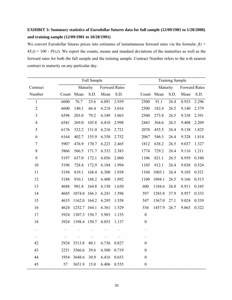
For the period 12/9/1981 to 1/28/2008, we obtain daily prices of all Eurodollar futures contracts listed
in the Chicago Mercantile Exchange.
The Eurodollar futures price on date t for maturity on date t + τ, P(τ;t), refers to 100 minus the
annualized 90-day Libor rate for the period t + τ to t + τ + 90. Since the CFRS [2008] model is built
around instantaneous forward rates, we make the simplifying assumption that the instantaneous forward
rate in the middle of the 90-day period referenced by the Eurodollar futures contract equals the annualized
forward rate implied by the Eurodollar futures price as the standard annualized discount rate: f(τ + 45;t) =
100 - P(τ;t).
Summary statistics of the implied forward rates are displayed in Exhibit 3. A typical day would see
approximately 40 active contracts, with the maximum being 45. The maturities of the forward rates range
from 45 days (corresponding to a Eurodollar futures contract that expires at the end of that trading day) to
slightly more than 10 years. The training sample, which is an early sub-sample of the data, is more
sparsely populated with an average of (approximately) 10 active contracts per trading day, with maturities
stretching out to 4 years.
**** EXHIBIT 3 AROUND HERE ****
One feature of the data that merits special attention is what appears to be a microstructure effect: there
are persistent blips in the data for December contracts, perhaps caused by those who use these contracts
for swaps. These blips occur systematically and our model – whose form and whose dynamics are both
smooth – cannot accommodate them. In order to build a useful model for prediction, we elected to
incorporate these microstructure features into the forecast. We describe this adjustment used in the section
titled Generating Model Forecasts.
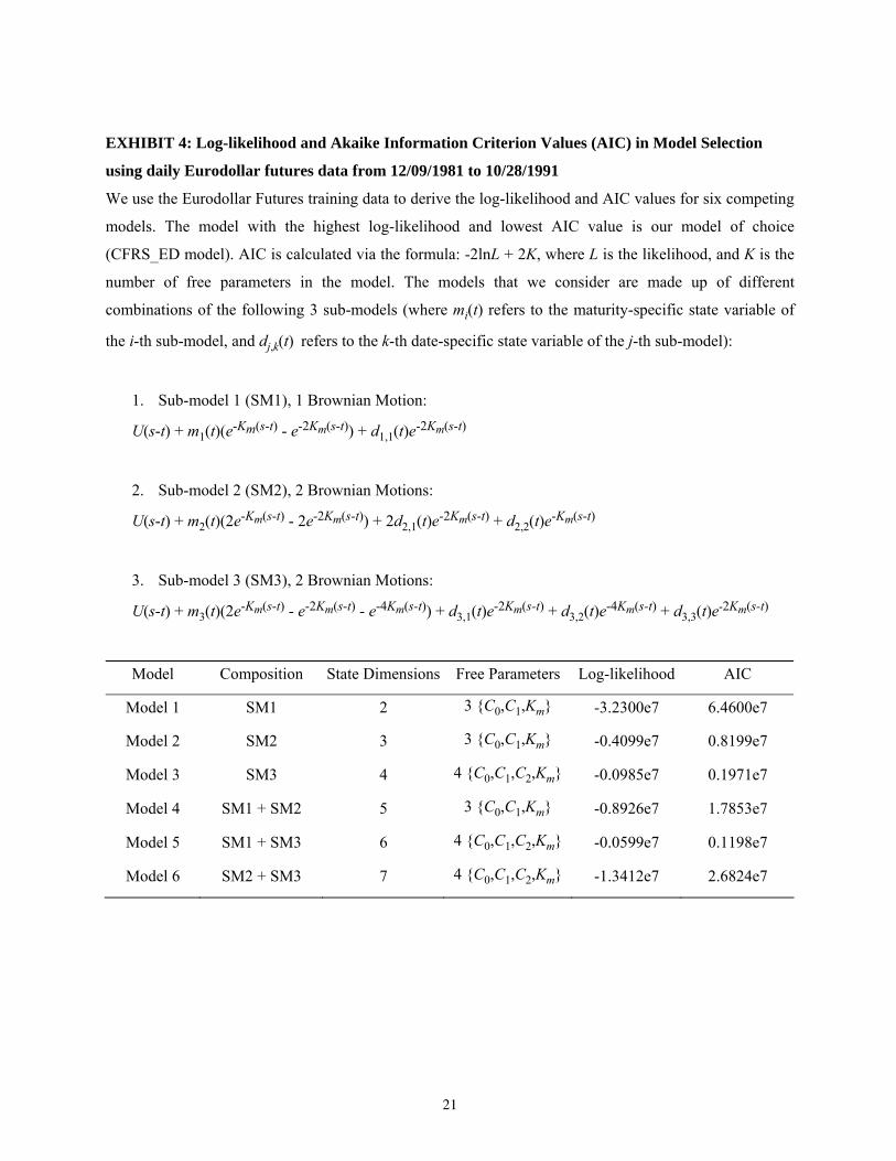
Model Selection using the AIC Criterion
In this section we describe the model we chose (from alternative parameterizations) and briefly
describe the procedure employed in that choice.
We restricted the alternative models to have no more than 4 Brownian Motions (BMs) that serve as
driving state variables. The advantage of our general model-building procedure is that we can bifurcate the
influence of each BM to impact the maturity-specific deviation, or the date-specific deviation, or both. In
10
this way we can permit the shape of the forward curve to accommodate several humps and also allow the
dynamics of the forward curve to be influenced by correlated deviations driven by independent BMs.
To choose from the list of alternative models, we fit each model over the period 12/09/1981 to
10/28/1991, using daily data from the Eurodollar futures market (2500 days of data). Each estimation
employs the Kalman filter in the manner explained in next section. The various alternative models are
generated by combining different sub-models (also referred to as arbitrage-free units or AFU, in CFRS
[2008]). CFRS [2008] also details the proof that combinations of these sub-models are arbitrage-free.
Because the alternative parameterizations involve forms with varying numbers of parameters, we used
the Akaike information criterion (henceforth AIC, see Akaike [1973]) to choose among the models.
Exhibit 4 shows the descriptions of the various candidate models and their respective AIC numbers.
Model 5 obtains the lowest AIC among the 6 candidate models. We therefore chose Model 5 (henceforth
CFRS_ED model) for empirical implementation reported in the rest of this paper.
**** EXHIBIT 4 AROUND HERE ****
The CFRS_ED model, driven by 3 independent Brownian motions, is the sum of the unconditional
curve, 2 maturity-specific curves, and 4 date-specific curves fitted to 3 exponential basis functions
{e-Km,e-2Km,e-4Km}. We denote the error term in the fitted model as ε(τ;t):
f(τ;t) = F3(τ;t) + ε(τ;t) (13)
so that
f(τ;t) = (e k rτ)' ( )u r + Mm r(t) + Dd r(t) + ε(τ;t) (14)
where
(e k rτ) =
⎣⎢⎡
⎦⎥⎤
1e-Kmτ
e-2Kmτ
e-4Kmτ
, M = ⎣⎢⎡
⎦⎥⎤
0 0 1 2 -1 -1 0 -1
, D = ⎣⎢⎡
⎦⎥⎤
0 0 0 0 0 0 0 0 1 1 0 1 0 0 1 0
11
m r(t) = ⎣⎢⎡
⎦⎥⎤
m1(t)m2(t) , d
r(t) =
⎣⎢⎢⎡
⎦⎥⎥⎤
d1(t)d2(t)d3(t)d4(t)
, u r =
⎣⎢⎢⎡
⎦⎥⎥⎤
C00
-C1-C2
Therefore there are 6 state variables in this system: m1(t), m2(t), d1(t), d2(t), d3(t) and d4(t).
The stochastic processes for vectors m r(t) and d r(t) are:
dm r(t) = Vm m r dt + Σm (m r) dB r(t) (15)
dd r(t) = Vd d
r dt + Σd (m r) dB
r(t) (16)
where
Vm = ⎣⎢⎡
⎦⎥⎤
-Km 00 -Km
, Vd =
⎣⎢⎢⎡
⎦⎥⎥⎤
-2Km 0 0 00 -2Km 0 00 0 -4Km 00 0 0 -2Km
Σm(m r) = ⎣⎢⎡
⎦⎥⎤
γ1,t 0 00 γ2,t 0
, Σd(m r) =
⎣⎢⎢⎡
⎦⎥⎥⎤
γ1,t 0 00 γ2,t 0
0 γ2,t 0 0 0 γ3,t
, dBt = ⎣⎢⎢⎡
⎦⎥⎥⎤
dB1,t
dB2,t dB3,t
using 3 independent Brownian motions, and
γ21,t = (m1(t)+C1)K 2
m
γ22,t = (m2(t)+C1)
K 2m
4
γ23,t = (3m2(t)+4C2)2K 2
m
12
Note that, in the model selection process, we limit the choice of models to those having at most 4 BMs
and a few alternative forms within that restriction; it is possible that more extensive forms may perform
better than our model in forecast accuracy.
Generating Model Forecasts
Suppose that on date T, we want to forecast future forward rates for date T2. We use a three-step
process:
1. Over the parameter space of {Km,σ*2}, (which are the rate of decay of the maturity-specific
deviations and the variance of the measurement errors of the Kalman filter, respectively) search
for a point that maximizes the quasi-likelihood. The quasi-likelihood for any point in the space is
obtained via the following procedure:
(a) Use all the data across dates and maturities for the Eurodollar forward rates, which we now
label as f(τ;t), for all dates up to date T to fit the unconditional forward curve of the form:
U(τ) = C0 - C1e-2Kmτ - C2e-4Kmτ
(b) Subtract the fitted unconditional forward curve from the observed forward rates to obtain the
cross-section of deviations. These deviations form the “observations” in the context of the
Kalman filter (The operations of the Kalman filter are detailed in the appendix):
z rt ≡ f( τ r;t) - U $( τ r) = Ax rt+ε r
t
(c) Run the Kalman filter to estimate the state variables for the maturity-specific and date-specific
curves.
(d) Determine the quasi-likelihood from the Kalman filter: lnL = - nT2 ln2π - 12 ∑
t=1
T (ln|Ht|+v'
t H -1t vt)
where Ht denotes the conditional covariance matrix of the prediction errors vt. See equation
(33) in the appendix.
2. Beginning with estimated state variables at date T obtained in the previous step, we evolve these
estimates forward according to their respective decay rates to obtain forecasts for future date T2:
m $1(T2) = E[m1(T2) | m $1(T)] = m $1(T)e-K $ m(T2-T) m $2(T2) = E[m2(T2) | m $2(T)] = m $2(T)e-K $ m(T2-T) d $1(T2) = E[d1(T2) | d $1(T)] = d $1(T)e-2K $m(T2-T)
13
d $2(T2) = E[d2(T2) | d $2(T)] = d $2(T)e-2K $m(T2-T) d $3(T2) = E[d3(T2) | d $3(T)] = d $3(T)e-4K $m(T2-T) d $4(T2) = E[d4(T2) | d $4(T)] = d $4(T)e-2K $m(T2-T)
3. Correct the model predictions to accommodate market microstructure effect (discussed above)
present at time T. Exhibit 5 illustrates the type of effects captured by the adjustment described
there. To that end, on the observed day T, we back out the forward curve using the current
estimates of the underlying state variables, obtaining a fitted curve. We then subtract this fitted
curve from the observed forward rates, producing ε(τ;T). Because this microstructure persists in
time, our forecast for the future data is f $(τ;T2) = (e k rτ)' ( )u r $ + Mm r $(T2) + Dd
r $(T2) + ε(τ + (T2-T);T).
In effect, we model the observed forward rates as a sum of the smooth curve implied by our
model plus additive microstructure effects. Our assumption is that the imprecise cross-sectional
fits are not measurement noise per se, which should dissipate over a longer term, but are market
micro-structure distortions that can be expected to persist over the short-term.
**** EXHIBIT 5 AROUND HERE ****
RESULTS
In this section, we test the efficacy of our forecasts using 2 different yardsticks: (1) the accuracy of
prediction of future forward rates implied by Eurodollar futures prices, as measured using RMSE; and (2)
the profitability of a simple trading strategy uses the predictions of the model to generate trade signals.
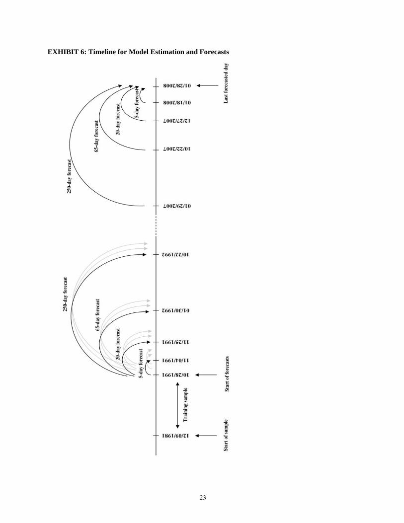
It should be emphasized that the model selection uses only data up to 10/28/1991 while forecast
generation, uses only the data that is available up to the date that the forecast is being made. This means
that the forecasts made are truly out-of-sample. We make forecasts for 5-trading-days, 20-trading-days,
65-trading-days and 250-trading-days ahead, approximately corresponding to 1-calendar-week, 1-
calendar-month, 1-calendar-quarter and 1-calendar-year ahead, respectively. Refer to Exhibit 6 to get a
graphical view of the model training and forecasting timeline.
**** EXHIBIT 6 AROUND HERE ****
14
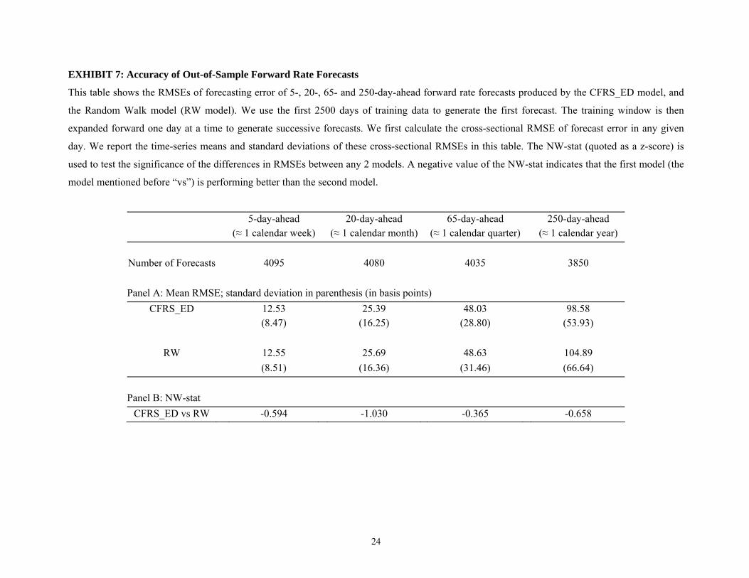
Predictive Accuracy
The forecast error are calculated as the differences between the forecasted forward rates and the actual
Eurodollar futures implied forward rates that prevail at the end of the forecasting period. We compare the
forecasts of the CFRS_ED model against the hypothesis that the Eurodollar futures prices of each contract
remains unchanged over the forecasting period, the random walk model (RW model). For each date, we
measure the cross-sectional square root of the mean squared forecast errors (RMSE). We report the time-
series average and standard deviation of these cross-sectional RMSEs in Panel A of Exhibit 7. We report
the statistical significance of the differences between the RMSE of the CFRS_ED model and the RW
model in Panel B of Exhibit 7.
The CFRS_ED model performs better than the random walk for all 4 forecast horizons, as evidenced
by the lower forecast error RMSEs. The differences in RMSE start from 0.02 basis points (12.53 for the
CFRS_ED model vs 12.55 for the RW model) for 5-day-ahead forecasts, and monotonically increase to an
economically significant 6.31 basis points for 250-day-ahead forecasts (98.58 for the CFRS_ED model
versus 104.89 for RW model). In terms of statistical significance, we calculate the Newey-West statistic
(NW-stat; see Newey and West [1987]) for the differences between the RMSE of the CFRS_ED model
and the RW model.6
The NW-stat takes into account serial correlation and heteroscedasticity in the time series of forecast
errors; this structure is very evident in our situation because of the over-lapping forecasting windows.
Panel B of Exhibit 7, shows that the CFRS_ED model is consistently more accurate, but the differences
are not statistically significant at the usual levels.
**** EXHIBIT 7 AROUND HERE ****
Trading Strategy Profitability
We use the methodology described above to generate forecasts and signals to trade forward rates 5-
days, 20-days, 65-days, and 250-days ahead. Each trade signal generated is based on whether the
forecasted forward rate is above or below the current Eurodollar-implied forward rate. If the forecasted
rate is below the current rate, we go short that forward rate (equivalently, we go long the Eurodollar
futures contract), and hold that short position until the end of the forecasting period. Conversely, if the
forecasted rate is above the current rate, we go long the that forward rate (by going short the Eurodollar
futures contract), and hold that long position until the end of the forecasting period. Trades are placed for
15
all Eurodollar futures contracts that will still exist at the end of the forecasting period. The profitability on
each trade is then calculated as the cross-sectional average movement in (or against) the predicted
direction over the length of the forecasting period, expressed in basis points. For comparison, we also
measure the profitability of an alternative trading strategy that always buys-and-holds a long position in
all the traded Eurodollar futures contracts, which is equivalent to riding the yield curve. We report the
means and standards deviations of the profitability of the CFRS_ED model trading strategy and the buy-
and hold strategy in Panel A of Exhibit 8. We report the statistical significance of the profitability of the
CFRS_ED model trading strategy, as well as the statistical significance of the differences in profitability
between the two strategies in Panel B of Exhibit 8.
In terms of profitability, the trading signals generated by the CFRS_ED model are significantly
positive, both economically and statistically. The average profit per trade ranges from 1.19 basis point for
the 5-day holding period strategy to 49.04 basis points for the 250-day holding period strategy. The
statistical significance of this profit, reported in row 1 of Panel B in Exhibit 8, as measured by the NW-
stat also exceeds the 5% level for all 4 holding periods.
Row 3 of Panel A in Exhibit 8 shows that the profitability of the buy-and-hold strategies, while
always lower than the CFRS_ED model, are quite similar in terms of magnitude. The buy-and-hold
strategy’s profits ranges from 1.16 basis point for the 5-day holding period strategy to 48.74 basis points
for the 250-day holding period strategy. The closeness between the profitability of these CFRS_ED model
and the buy-and-hold is reflective of the fact that the CFRS_ED model will, more often than not, predict a
fall in forward rates, due to the fact that unconditionally, the term structure of the forward curve is upward
sloping (hence, unconditionally, the drift of forward rates is downwards). The differences in profitability
will therefore come from the times when the CRFS_ED model predicts a rise in the forward rates, while
the buy-and-hold maintains the downward prediction. Hence, to test the statistical significance between
the CFRS_ED model and the buy-and-hold model, we exclude all the dates when the trade signals are
identical for both strategies, and only use those dates when their forecasted directions diverge.
Row 2 of Panel B of Exhibit 8 shows that the profitability of the CFRS_ED model is significantly
higher than that for the buy-and-hold for all holding periods, and especially so for the 65-day and 250-day
holding periods, with NW-stat reaching 7.953.
**** EXHIBIT 8 AROUND HERE ****
16
CONCLUSION
We have estimated and tested a dynamic model for the forward Eurodollar rates. The model has
several desirable features, most notably that it
• Captures maturity-specific preferences that arise from preferred habitats,
• Accommodates date-specific expectations about future spot rates,
• Permits estimation and extrapolation via underlying state variables within the framework of a
Kalman filter, and
• Has a general structure that permits the choice of a particular model parsimonious in parameters
and state variables, while still remaining arbitrage-free.
The selected representative of our model class performs well in forecasts over various horizons,
relative to the Random Walk model. The chosen model also supports the construction of a trading strategy
that significantly outperforms the returns of a buy-and-hold strategy, especially over longer holding
periods.
We leave to future work the task of searching for the superior models from this general class as well
as the extension to other types of data.
17
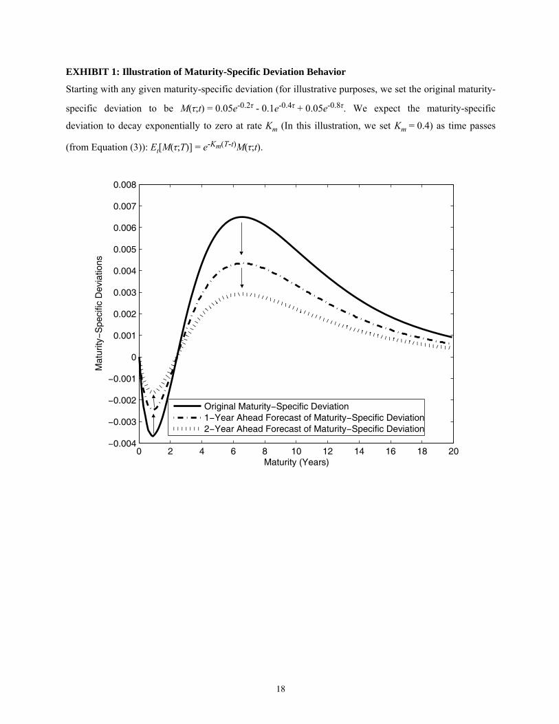
EXHIBIT 1: Illustration of Maturity-Specific Deviation Behavior
Starting with any given maturity-specific deviation (for illustrative purposes, we set the original maturity-
specific deviation to be M(τ;t) = 0.05e-0.2τ - 0.1e-0.4τ + 0.05e-0.8τ. We expect the maturity-specific
deviation to decay exponentially to zero at rate Km (In this illustration, we set Km = 0.4) as time passes
This table shows the profitability of trading strategies that capitalizes on the forecasts of the CFRS_ED model, as well as a buy-and-hold model.
We consider trading strategies over a 5-, 20-, 65- and 250-day holding period. We use the first 2500 days of training data to generate the first
forecast. The training window is then expanded forward one day at a time to generate successive forecasts. If the forecasted forward rate is lower
(higher) than the current corresponding forward rate, the strategy is to bet that the forward rate will fall (rise) over the forecasted period. Trades are
placed for all Eurodollar futures contracts that will still exist at the end of the forecasting period. The profitability on each trade is then calculated
as the cross-sectional average movement in (or against) the predicted direction over the length of the forecasting period, expressed in basis points.
We report the time-series means and standard deviations of the cross-sectional average. The NW-stat (quoted as a z-score) is used to test the
significance of the differences in profitability between any 2 trading strategies, using only days when the trades of the 2 strategies are different. A
positive value of the NW-stat indicates that the first strategy (the model mentioned before “vs”) is performing better than the second strategy.
5-day holding period 20-day holding period 65-day holding period 250-day holding period (≈ 1 calendar week) (≈ 1 calendar month) (≈ 1 calendar quarter) (≈ 1 calendar year)
Number of Forecasts 4095 4080 4035 3850
Panel A: Mean Profitability; standard deviation in parenthesis (in basis points)
Vasicek, O. “An Equilibrium Characterization of the Term Structure.” Journal of Financial Economics, 5
(1977), 177–188.
31
ENDNOTES
1The CFRS model does not account for default and (strictly speaking) applies to forward rates implicit in
Treasury yields. The Eurodollar futures market settles to the rate on dollar-denominated inter-bank loans in London and therefore is affected by a credit risk; we choose it because is a very liquid market and offers a rich source of data.
2Some recent literature seem to vindicate theoretical aspects of the Expectations Hypothesis. McCulloch [1993] and Fisher and Gilles [1998] present examples to show that some forms of the Expectations Hypothesis are consistent with no-arbitrage. Longstaff [2000] shows that all traditional forms of the Expectations Hypothesis are consistent with no-arbitrage if markets are incomplete.
3See CFRS [2008] for further discussion of the connection of their model to other models. 4The instantaneous forward rate on date t for maturity on date s is really a function of {t,s-t,m(t), and d(t)}
where the final two arguments are state variables that affect the maturity- and date-specific deviations. For simplicity, we will continue to write our model for the forward rate as a function of 2 variables: {τ = s-t,t}, writing F1(τ;t) in place of F1(t,s,m(t),d(t)) and suppressing the dependence on the two state variables.
5The precise choice of exponential bases can affect the arbitrage-free status of the model, making it important to verify the HJM conditions for each choice.
6We first compute the difference between a given day’s cross-sectional RMSE for our model and the RW model. Then, we compute the Newey-West (NW) standard error for the time-series of these differences. The mean difference divided by this NW standard error is our reported NW statistic. Alternatively, we can compute the significance using the Diebold-Mariano [1995] method.
7It is not necessary that κt= γ
tK
m. If the market price of risk takes on another form, the model requires a different
specification for γt or U(s-t) or both so that the system remains arbitrage-free. 8The framework of the model places boundaries on the values of some of the state variables. The diffusion
terms, which are functions of the maturity-specific state variables, must be constrained to be non-negative. This in turn places constraints on those state variables. In the empirical implementation, a simple and common way of enforcing this restriction is to replace the values of the state variables that do breach the constraints with ones that just satisfy it. See Chen and Scott [2002] and Geyer and Pichler [1999] for further examples of such restrictions in a Kalman filter.