Article

Predicting Stem Total and Assortment Volumes inan Industrial Pinus taeda L. Forest Plantation UsingAirborne Laser Scanning Data and Random Forest

Carlos Alberto Silva 1,2,3,*, Carine Klauberg 2, Andrew Thomas Hudak 2, Lee Alexander Vierling 1,Wan Shafrina Wan Mohd Jaafar 4, Midhun Mohan 5, Mariano Garcia 6 ID , António Ferraz 3,Adrián Cardil 7 and Sassan Saatchi 3

1 Department of Natural Resources and Society, College of Natural Resources, University of Idaho (UI),875 Perimeter Drive, Moscow, ID 83843, USA; leev@uidaho.edu

2 US Forest Service (USDA), Rocky Mountain Research Station, RMRS, 1221 South Main Street, Moscow,ID 83843, USA; carine_klauberg@hotmail.com (C.K.); ahudak@fs.fes.us (A.T.H.)

3 Jet Propulsion Laboratory, California Institute of Technology 4800 Oak Grove Drive, Pasadena, CA 91109,USA; ferraz.antonio.a@gmail.com (A.F.); sasan.s.saatchi@jpl.nasa.gov (S.S.)

4 School of Geosciences, University of Edinburgh, Edinburgh EH8 9XL, UK; wanshafrina@gmail.com5 Department of Forestry and Environmental Resources, North Carolina State University, 2800 Faucette Drive,

Raleigh, NC 27695, USA; mmohan2@ncsu.edu6 Centre for Landscape and Climate Research, Department of Geography, University of Leicester,

Leicester LE1 7RH, UK; mariano.gar.alo@gmail.com7 Tecnosylva Parque Tecnológico de León, 24009 León, Spain; adriancardil@gmail.com* Correspondence: carlos_engflorestal@outlook.com; Tel.: +1-(208)-5964510

Academic Editor: Timothy A. MartinReceived: 27 April 2017; Accepted: 13 July 2017; Published: 17 July 2017

Abstract: Improvements in the management of pine plantations result in multiple industrial andenvironmental benefits. Remote sensing techniques can dramatically increase the efficiency ofplantation management by reducing or replacing time-consuming field sampling. We tested the utilityand accuracy of combining field and airborne lidar data with Random Forest, a supervised machinelearning algorithm, to estimate stem total and assortment (commercial and pulpwood) volumes in anindustrial Pinus taeda L. forest plantation in southern Brazil. Random Forest was populated usingfield and lidar-derived forest metrics from 50 sample plots with trees ranging from three to nine yearsold. We found that a model defined as a function of only two metrics (height of the top of the canopyand the skewness of the vertical distribution of lidar points) has a very strong and unbiased predictivepower. We found that predictions of total, commercial, and pulp volume, respectively, showed anadjusted R2 equal to 0.98, 0.98 and 0.96, with unbiased predictions of −0.17%, −0.12% and −0.23%,and Root Mean Square Error (RMSE) values of 7.83%, 7.71% and 8.63%. Our methodology makes useof commercially available airborne lidar and widely used mathematical tools to provide solutions forincreasing the industry efficiency in monitoring and managing wood volume.

Keywords: forest inventory; lidar; remote sensing; supply chain

1. Introduction

The area of planted forests worldwide has been steadily growing, with an estimated 6.95%of total global forested area being plantations in 2010 [1]. Tropical regions may be experiencingparticularly rapid rates of plantation expansion [2]. For example, the area of pine plantations in Brazilhas dramatically risen in the last few decades to increase pulp and paper production. Currently ~20%of the total reforested area of Brazil is comprised of pine forest plantations [2].

Forests 2017, 8, 254; doi:10.3390/f8070254 www.mdpi.com/journal/forests

Forests 2017, 8, 254 2 of 17

Most of the pine plantations are concentrated in South Brazil, with 34.1% and 42.4% of the totalreforested area located in Paraná and Santa Catarina states [2]. Pinus taeda L., also known as loblollypine, is the most planted forest specie in these regions. It has high economic importance due to itshigh volumetric increment in the colder regions of the southern Brazil [3]. It has fast growing ratespresenting increments up to 50 m3·ha−1·year−1 [2]. Moreover, P. taeda is commonly managed forproduction of multiple types of wood such as stem total, saw logs, pulpwood and small-diameter logsand branches, which are used for energy. Saw logs and pulpwood can be further divided into differentassortments that differ in size and therefore in economic value [3].

Forest inventory in P. taeda is currently based on field measurements and typically conductedannually to monitor forest growth in Brazil, allowing managers to identify problematic conditionsduring initial growth stages, and determine optimal harvest time [4]. While field measurements areconsidered the most accurate approach for monitoring industrial forest plantations, measuring stemtotal and assortment volumes annually via traditional methods is an extremely time consuming andlabor-intensive task, especially in large plantations where a huge number of plots need to be measuredto characterize the variation [5]. Hence, to improve plantation management there is a need to developand implement accurate, repeatable, and economical remote sensing based methods that providesynoptic coverage at high spatial resolution.

Over the past few decades, lidar remote sensing has been established as one of the promising andprimary tools for broad-scale analysis of forest systems. Lidar data can be used to characterize local toregional spatial extents with high enough resolution to quantify the three-dimensional structure of theforest with the support of efficiently collected field data and several statistical methods (e.g., [6–10]).Lidar can be used to produce highly accurate retrievals of tree density, stem total and assortment volumes,basal area, aboveground carbon, and leaf area index, and thereby can be an effective way to predict andmap forest attributes at unsampled locations (e.g., [11–16]). To parlay these attributes into improvedforest management practices for wood and pulp production, it is often necessary to predict stem totaland assortment volumes of pine plantations in operational and experimental scenarios, as these scenariosoften include thinning cruises, mid-rotation cruises, genetic trials, and silviculture research tests [17].

Current predictive modeling methods include parametric (e.g., multiple linear regression) andnon-parametric (e.g., Random Forest) approaches (e.g., [6,7,18]). Among the machine learning algorithms,the Random Forest (RF) modeling approach has gained popularity in estimating forest attributes fromlidar data due to its flexibility and ability to maintain nonlinear dependences compared to parametricalgorithms [19]. The RF can be viewed as an improved version of classification and regression tree (CART)methods; data and variables can be randomly sampled by RF in an iterative bagging bootstrap procedureto generate a “forest” of regression trees [20]. Also, incorporation of multiple decision trees and internalcross-validation has improved results, enhanced ease of use and reduced issues regarding over-fittingwhile performing this modeling approach [21,22]. In case of regression-type problems, RF acts as anarbitrary number of simple trees whose responses are averaged to obtain an estimate of dependentvariables [23]. Diversification of sample trees is primarily done in two ways, either through a balancingmethodology where equal numbers of samples are drawn from minority classes and majority classes,or by assigning a higher weight (i.e., heavier penalty) on misclassified minority class and taking themajority voting of individual classification trees [24]. As RF does not require any assumptions aboutthe relationships between explanatory and response variables, they are considered well suited foranalyzing complex non-linear and possibly hierarchical interactions in large datasets [25]. In forestinventory, RF has been used for predicting and mapping forest attribute at the stand (e.g., [19]) andindividual tree levels [23], in addition to disturbance evaluation (e.g., [26]), mapping invasive plantspecies (e.g., [27]), and vegetation classification (e.g., [21]). Despite of the above-mentioned studies, toour knowledge, lidar and RF have been not yet been combined for predicting and mapping stem total,saw log and pulpwood volumes in industrial P. taeda forest plantations at stand level.

Timely monitoring of stem total and assortment volumes in P. taeda plantations with lidar dataand RF would allow managers to determine the optimal time for harvest or other treatment activities

Forests 2017, 8, 254 3 of 17

to maximize economic return. Therefore, the development of robust frameworks for modeling andmapping stem total and assortment volumes at plot and stand levels is still needed to increase theefficiency in monitoring and managing wood and pulp productions in forest plantations. Moreover,efficient frameworks also play important role in helping lidar technology move from research tooperational modes, especially in industrial forest plantation settings where lidar applications arerelatively new. The aims of this study were to: (i) present a robust and efficient framework formodeling, predicting and mapping stem total volume (Vt), saw logs (in this study mentioned ascommercial) volume (Vc) and pulpwood volume (Vp) in a P. taeda plantation in southern Brazil usingairborne lidar data; (ii) evaluate the use of the RF machine learning algorithm for modeling stem totaland assortment volumes; and (iii) generate maps representing the spatial distribution of Vt, Vc and Vpin differently aged plantations of P. taeda. This investigation was based on the hypothesis that lidartechnology and Random Forest analysis can facilitate accurate and precise inferences of forest volumesin P. taeda plantations in southern Brazil.

2. Methods

2.1. Study Area Description

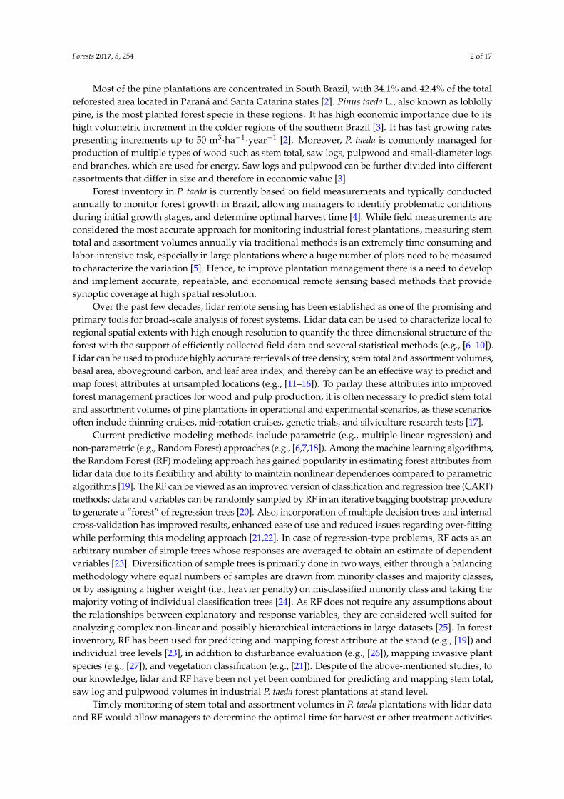
The study area consisted of P. taeda stands located within the Telêmaco Borba municipality in thestate of Paraná, southern of Brazil (Figure 1). Trees were planted using a 3.0 × 2.0 m or 2.5 × 2.5 m gridconfiguration, resulting in an average tree density of 1667 or 2000 trees ha−1, respectively. The climateof the region is characterized as warm and temperate [28], with annual average precipitation ofapproximately 1378 mm and an annual average temperature of 18.4 ◦C. The P. taeda stands are situatedon a plateau where the topography is relatively flat. The plantations are managed by Klabin S.A.,a pulp and paper company.

Forests 2017, 8, 254 3 of 17

to maximize economic return. Therefore, the development of robust frameworks for modeling and mapping stem total and assortment volumes at plot and stand levels is still needed to increase the efficiency in monitoring and managing wood and pulp productions in forest plantations. Moreover, efficient frameworks also play important role in helping lidar technology move from research to operational modes, especially in industrial forest plantation settings where lidar applications are relatively new. The aims of this study were to: (i) present a robust and efficient framework for modeling, predicting and mapping stem total volume (Vt), saw logs (in this study mentioned as commercial) volume (Vc) and pulpwood volume (Vp) in a P. taeda plantation in southern Brazil using airborne lidar data; (ii) evaluate the use of the RF machine learning algorithm for modeling stem total and assortment volumes; and (iii) generate maps representing the spatial distribution of Vt, Vc and Vp in differently aged plantations of P. taeda. This investigation was based on the hypothesis that lidar technology and Random Forest analysis can facilitate accurate and precise inferences of forest volumes in P. taeda plantations in southern Brazil.

2. Methods

2.1. Study Area Description

The study area consisted of P. taeda stands located within the Telêmaco Borba municipality in the state of Paraná, southern of Brazil (Figure 1). Trees were planted using a 3.0 × 2.0 m or 2.5 × 2.5 m grid configuration, resulting in an average tree density of 1667 or 2000 trees ha−1, respectively. The climate of the region is characterized as warm and temperate [28], with annual average precipitation of approximately 1378 mm and an annual average temperature of 18.4 °C. The P. taeda stands are situated on a plateau where the topography is relatively flat. The plantations are managed by Klabin S.A., a pulp and paper company.

Figure 1. Location of study area in Telêmaco Borba, Paraná, Brazil. The black dotes indicate the location of the Pinus teada stands.

2.2. Field Data Collection

A total of 50 rectangular plots, each approximately 600 m2 (i.e., 20 m × 30 m) were randomly established and measured across 50 stands distributed in four plantations. As such, the sample plots

Figure 1. Location of study area in Telêmaco Borba, Paraná, Brazil. The black dotes indicate the locationof the Pinus teada stands.

2.2. Field Data Collection

A total of 50 rectangular plots, each approximately 600 m2 (i.e., 20 m × 30 m) were randomlyestablished and measured across 50 stands distributed in four plantations. As such, the sample plots

Forests 2017, 8, 254 4 of 17

well represent the study area, and they capture the entire structural variability in these stands withages ranging from three to nine years old. All plots were geo-referenced with a geodetic GPS withdifferential correction capability (Trimble Pro-XR, Trimble, Sunnyvale, CA, USA) ensuring a locationerror lower than 10 cm. In each sample plot, individual trees were measured for dbh (diameter atbreast height) at 1.30 m and a random subsample (15%) of trees for tree height (Ht). For those trees inthe plots that were not directly measured for Ht, the inventory team of Klabin S.A. predicted heightsfrom hypsometric equations [29], employing dbh as the independent variable, and Ht as the dependentvariable, following the model below:

ln(Ht) = β0 + β1 × (1/dbh) + e (1)

where ln(Ht) is the natural logarithm of tree height (m); β0 and β1 are the intercept and the slopeof the model; dbh is the diameter at breast height (1.30 m) and e is the random error of the model.The coefficients of the hypsometric models are the companies intellectual property and not madeavailable to the public, however, the adjusted coefficient of determination (adj. R2) and standard errorof estimate in percentage (SEE%) of the models ranged from 0.96 to 0.98 and 5.1 to 6.5, respectively.

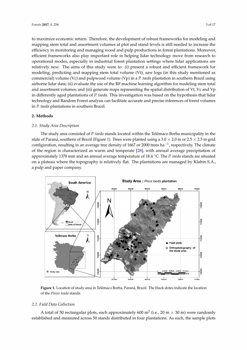
The management goal of the P. taeda plantations at Klabin is optimized to produce commerciallogs of 2.65 m in length, which are then classified in four timber assortment classes: 18 to 25 cm (Vc 1),25 to 30 cm (Vc 2), 30 to 40 cm (Vc 3), and diameter ≥ 40 cm (Vc 4). The logs designated for pulpwoodare produced with log lengths of 2.40 m and diameters ranging from 8 to 18 cm (Vp), as illustrated inFigure 2.

Forests 2017, 8, 254 4 of 17

well represent the study area, and they capture the entire structural variability in these stands with ages ranging from three to nine years old. All plots were geo-referenced with a geodetic GPS with differential correction capability (Trimble Pro-XR, Trimble, Sunnyvale, CA, USA) ensuring a location error lower than 10 cm. In each sample plot, individual trees were measured for dbh (diameter at breast height) at 1.30 m and a random subsample (15%) of trees for tree height (Ht). For those trees in the plots that were not directly measured for Ht, the inventory team of Klabin S.A. predicted heights from hypsometric equations [29], employing dbh as the independent variable, and Ht as the dependent variable, following the model below: ln(Ht) = β + β × (1/dbh) + e (1)

where ln(Ht) is the natural logarithm of tree height (m); β and β are the intercept and the slope of the model; dbh is the diameter at breast height (1.30 m) and e is the random error of the model. The coefficients of the hypsometric models are the companies intellectual property and not made available to the public, however, the adjusted coefficient of determination (adj. R2) and standard error of estimate in percentage (SEE%) of the models ranged from 0.96 to 0.98 and 5.1 to 6.5, respectively.

The management goal of the P. taeda plantations at Klabin is optimized to produce commercial logs of 2.65 m in length, which are then classified in four timber assortment classes: 18 to 25 cm (Vc 1), 25 to 30 cm (Vc 2), 30 to 40 cm (Vc 3), and diameter ≥ 40 cm (Vc 4). The logs designated for pulpwood are produced with log lengths of 2.40 m and diameters ranging from 8 to 18 cm (Vp), as illustrated in Figure 2.

Figure 2. Process of forest volume mesurement. (A) Pinus plantation; (B) Timber harvester and (C) Log segmentation for classes of volume mesurements.

In this study, Vt, Vc and Vp for each tree were computed using the fifth-degree polynomial [30] as presented below: ddbh = β + β hh + β hh + β hh + β hh + β hh (2)

V = K d δh (3)

Figure 2. Process of forest volume mesurement. (A) Pinus plantation; (B) Timber harvester and (C) Logsegmentation for classes of volume mesurements.

In this study, Vt, Vc and Vp for each tree were computed using the fifth-degree polynomial [30]as presented below:

di

dbh=

⌊β0 + β1

(hi

h

)+ β2

(hi

h

)2+ β3

(hi

h

)3+ β4

(hi

h

)4+ β5

(hi

h

)5⌋

(2)

V = K∫ h2

h1

d2i δh (3)

Forests 2017, 8, 254 5 of 17

V = K dbh2∫ h2

h1

(β0 + β1/h × h11 + β2/h2 × h2

2 + β3/h3 × h32 + β4/h4 × h4

2 + β5/h5 × h52)

2δh (4)

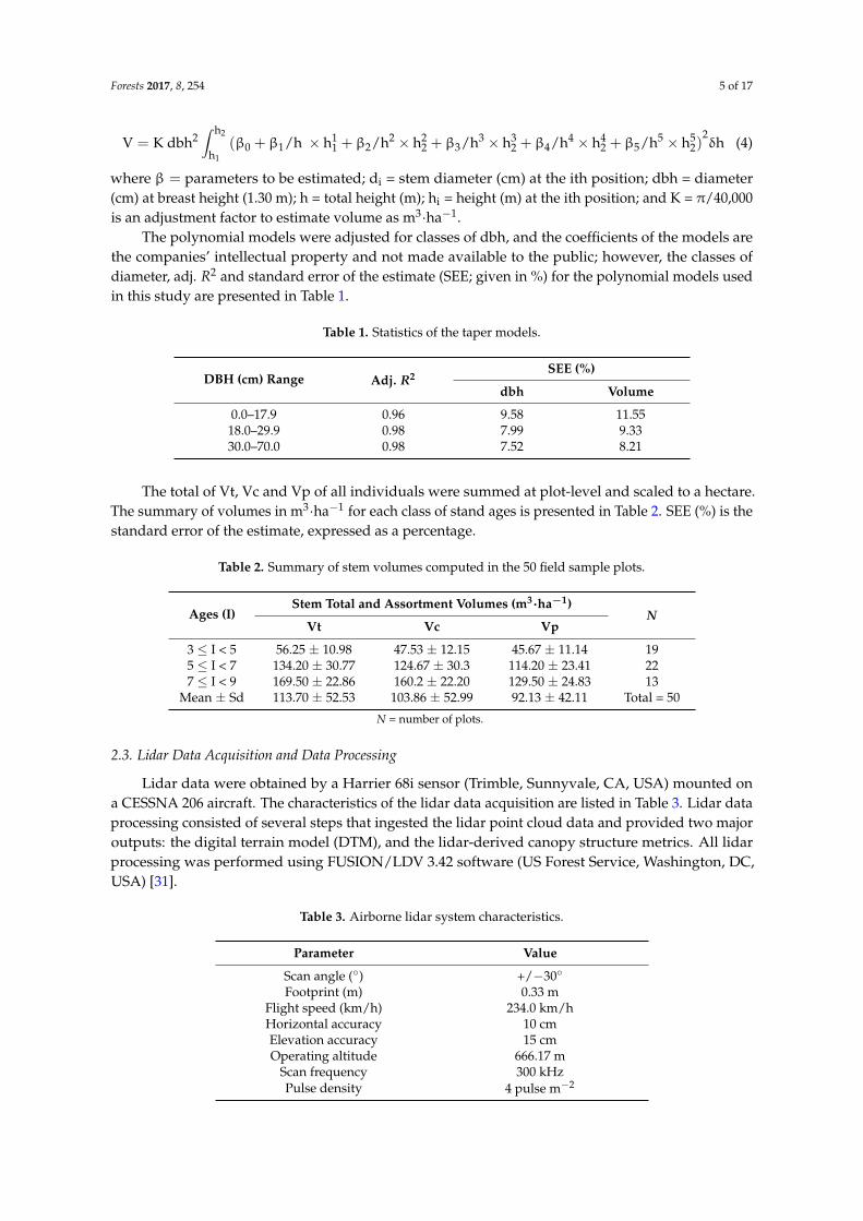
where β = parameters to be estimated; di = stem diameter (cm) at the ith position; dbh = diameter(cm) at breast height (1.30 m); h = total height (m); hi = height (m) at the ith position; and K = π/40,000is an adjustment factor to estimate volume as m3·ha−1.

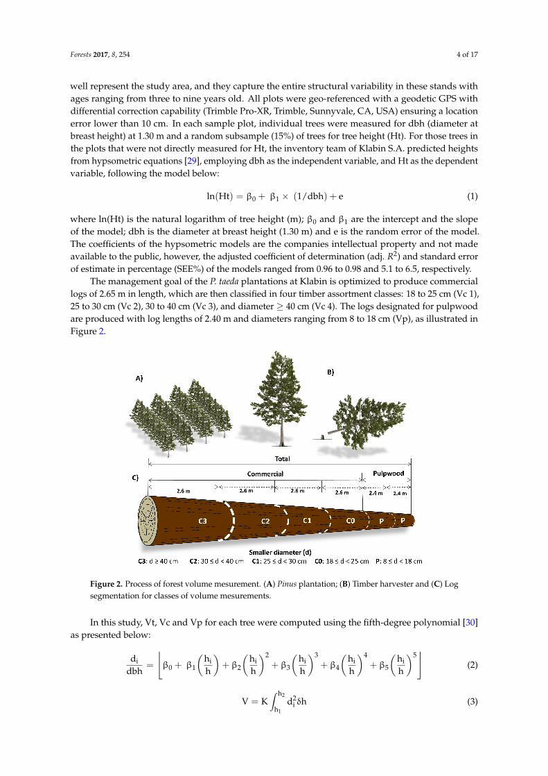
The polynomial models were adjusted for classes of dbh, and the coefficients of the models arethe companies’ intellectual property and not made available to the public; however, the classes ofdiameter, adj. R2 and standard error of the estimate (SEE; given in %) for the polynomial models usedin this study are presented in Table 1.

Table 1. Statistics of the taper models.

DBH (cm) Range Adj. R2SEE (%)

dbh Volume

0.0–17.9 0.96 9.58 11.5518.0–29.9 0.98 7.99 9.3330.0–70.0 0.98 7.52 8.21

The total of Vt, Vc and Vp of all individuals were summed at plot-level and scaled to a hectare.The summary of volumes in m3·ha−1 for each class of stand ages is presented in Table 2. SEE (%) is thestandard error of the estimate, expressed as a percentage.

Table 2. Summary of stem volumes computed in the 50 field sample plots.

Ages (I)Stem Total and Assortment Volumes (m3·ha−1)

NVt Vc Vp

3 ≤ I < 5 56.25 ± 10.98 47.53 ± 12.15 45.67 ± 11.14 195 ≤ I < 7 134.20 ± 30.77 124.67 ± 30.3 114.20 ± 23.41 227 ≤ I < 9 169.50 ± 22.86 160.2 ± 22.20 129.50 ± 24.83 13

Mean ± Sd 113.70 ± 52.53 103.86 ± 52.99 92.13 ± 42.11 Total = 50

N = number of plots.

2.3. Lidar Data Acquisition and Data Processing

Lidar data were obtained by a Harrier 68i sensor (Trimble, Sunnyvale, CA, USA) mounted ona CESSNA 206 aircraft. The characteristics of the lidar data acquisition are listed in Table 3. Lidar dataprocessing consisted of several steps that ingested the lidar point cloud data and provided two majoroutputs: the digital terrain model (DTM), and the lidar-derived canopy structure metrics. All lidarprocessing was performed using FUSION/LDV 3.42 software (US Forest Service, Washington, DC,USA) [31].

Table 3. Airborne lidar system characteristics.

Parameter Value

Scan angle (◦) +/−30◦

Footprint (m) 0.33 mFlight speed (km/h) 234.0 km/hHorizontal accuracy 10 cmElevation accuracy 15 cmOperating altitude 666.17 m

Scan frequency 300 kHzPulse density 4 pulse m−2

Forests 2017, 8, 254 6 of 17

The original point cloud data were filtered using Kraus and Pfeifer’s algorithm [32] and a 1 mresolution DTM was generated from the points classified as ground. Subsequently, the height of thereturns was computed by subtracting the elevation of the DTM from each return. Once the heightswere normalized, the metrics shown in Table 4 were computed at plot and stand levels, at a grid cellresolution of 25 m, using all lidar returns.

Table 4. Lidar-derived canopy height metrics considered as candidate variables for predictive Vmodels [31].

Variable Description

HMIN Height MinimumHMAX Height Maximum

HMEAN Height MeanHMAD Height median absolute deviation

HSD Height standard deviationHSKEW Height skewnessHKURT Height kurtosis

HCV Height coefficient of variationHIQ Height interquartile range

HMODE Height modeH01TH Height 1th percentileH05TH Height 5th percentileH10TH Height 10th percentileH15TH Height 15th percentileH20TH Height 20th percentileH25TH Height 25th percentileH30TH Height 30th percentileH35TH Height 35th percentileH40TH Height 40th percentileH45TH Height 45th percentileH50TH Height 50th percentileH55TH Height 55th percentileH60TH Height 60th percentileH65TH Height 65th percentileH70TH Height 70th percentileH75TH Height 75th percentileH80TH Height 80th percentileH90TH Height 90th percentileH95TH Height 95th percentileH99TH Height 99th percentile

CR Canopy Relief Ratio ((HMEAN − HMIN)/(HMAX − HMIN))COV Canopy Cover (Percentage of first return above 1.30 m)

2.4. Predictor Variables Selection

In order to derived accurate estimates of stem volumes from lidar, it is essential to select the mostsignificant lidar metrics (predictor variables) for modeling within a parsimonious statistical modelframework. Because the number of candidate lidar metrics can be very large (e.g., 30 metrics), inour study we selected the best lidar metrics for modeling stem volumes based on two steps. First,even though highly correlated variables will not cause multi-collinearity issues in RF [20], Pearson’scorrelation (r) was used to identify highly correlated predictor variables (r > 0.9) as presented inprevious studies (e.g., [14,33,34]). If a given group (2 or more) of lidar metrics were highly correlated,we retained only one metric by excluding the others that were most highly correlated with theremaining metrics. Second, we identified the most important metrics based on the Model ImprovementRatio (MIR), a standardized measure of variable importance [35,36]. MIR scores are derived by dividingraw variable important scores (output from RF models) by the maximum variable importance score,so that MIR values range from 0 to 1. MIR scores allow for variable importance comparisons among

Forests 2017, 8, 254 7 of 17

different RF models. We ran the RF routine (package randomForest [37]) in R [38] 1000 times tocompute MIR. In each MIR iteration, we bootstrapped the data by randomly selecting a sample of50 plots with replacement. RF requires two parameters to be set: (i) mtry, the number of predictorvariables performing the data partitioning at each node which in this study was defined by the numberof highly uncorrelated preliminary set of lidar metrics and (ii) ntree, the total number of trees to begrown in the model run which was set to 1000 (e.g., [34,39]). Running 1000 iterations of RF producedconsistent MIR distributions and avoided unnecessary processing time [39]. To create parsimoniousmodels, we reserved the metrics for final RF models that exhibited the highest mean MIR values.

2.5. Random Forest Model Development

The three stem volumes (Vt, Vc and Vp) of interest were predicted at the plot and stand-levelsusing also the RF package [37] in R [38]. The number of RF trees to grow was set to 1000, and thenumber of predictor variables performing the data partitioning at each node was set to equal thenumber of best lidar metrics selected by MIR on Section 2.4 [37]. The accuracy of estimates for eachmodel was evaluated in terms of Adj. R2, Root Mean Square Error (RMSE), and Bias (both absolute andrelative) by the linear relationship between predicted (output from RF) and observed stem volumes:

RMSE (m3·ha−1) =

√√√√ n

∑i=1

(yi − yi)2

/n (5)

Bias (m3·ha−1) =1n

n

∑i=1

(yi − yi) (6)

where n is the number of plots, yi is the observed value for plot i, and yi is the predicted value forplot i. Moreover, relative RMSE (%) and biases (%) were calculated by dividing the absolute values(Equations (5) and (6)) by the mean of the observed stem volume. Based on earlier experiences andrecommendations from literature [4,5], we defined acceptable model accuracy as a relative RMSE andBias of <15%.

For validation purposes, RF models were embedded in a bootstrap with 500 iterations. In eachbootstrap iteration, we drew 50 times with replacement from the 50 available samples. In thisprocedure, on average 44% of the total of sample (~22 samples) are not drawn. These sampleswere subsequently used as holdout samples for an independent validation (e.g., [40]). In eachbootstrap iteration, Adj. R2, absolute and relative RMSE and Bias were computed based on thelinear relationship between observed and predicted volumes using the holdout samples. We used alsotwo-sided Kolmogorov-Smirnov (KS) in R [38] and a statistical equivalence test [41] to compare thefield- and lidar-based stem volume estimates in each iteration.

2.6. Predictive Stem Volumes Maps

Predictive maps of stem volumes at 25 m of spatial resolution were generated based on the RFmodels containing the best lidar metrics according to MIR analysis. Because we have a large numberof stands in this study, stem volumes predictions at the stand level were then presented herein bystand ages of 3–5, 5–7 and 7–9 years. Additionally, maps of coefficient of variation (CV, given in %)values for the stem volume predictions (as obtained from the 500 bootstrap runs) was also producedfor each stand (e.g., [40]). Figure 3 provides an overview of the study methodology.

Forests 2017, 8, 254 8 of 17

Forests 2017, 8, 254 8 of 17

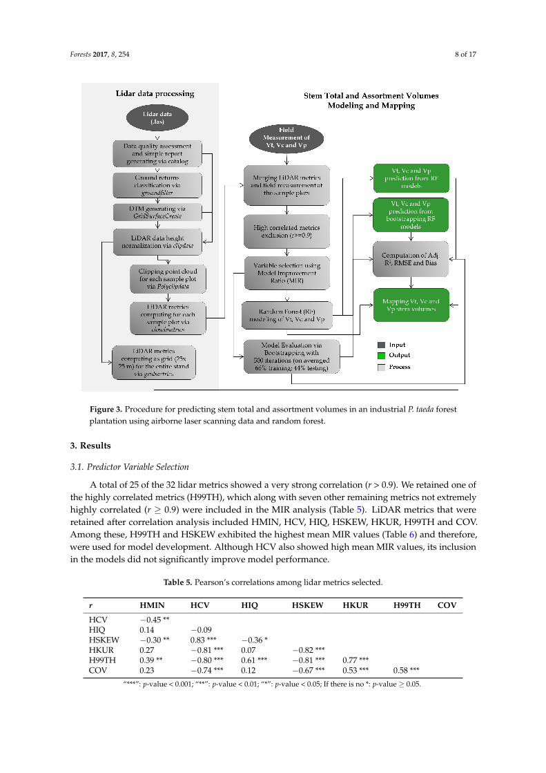
Figure 3. Procedure for predicting stem total and assortment volumes in an industrial P. taeda forest plantation using airborne laser scanning data and random forest.

3. Results

3.1. Predictor Variable Selection

A total of 25 of the 32 lidar metrics showed a very strong correlation (r > 0.9). We retained one of the highly correlated metrics (H99TH), which along with seven other remaining metrics not extremely highly correlated (r ≥ 0.9) were included in the MIR analysis (Table 5). LiDAR metrics that were retained after correlation analysis included HMIN, HCV, HIQ, HSKEW, HKUR, H99TH and COV. Among these, H99TH and HSKEW exhibited the highest mean MIR values (Table 6) and therefore, were used for model development. Although HCV also showed high mean MIR values, its inclusion in the models did not significantly improve model performance.

Table 5. Pearson’s correlations among lidar metrics selected.

r HMIN HCV HIQ HSKEW HKUR H99TH COV HCV −0.45 ** HIQ 0.14 −0.09 HSKEW −0.30 ** 0.83 *** −0.36 * HKUR 0.27 −0.81 *** 0.07 −0.82 *** H99TH 0.39 ** −0.80 *** 0.61 *** −0.81 *** 0.77 *** COV 0.23 −0.74 *** 0.12 −0.67 *** 0.53 *** 0.58 ***

“***”: p-value < 0.001; “**”: p-value < 0.01; “*”: p-value < 0.05; If there is no *: p-value > 0.05.

Figure 3. Procedure for predicting stem total and assortment volumes in an industrial P. taeda forestplantation using airborne laser scanning data and random forest.

3. Results

3.1. Predictor Variable Selection

A total of 25 of the 32 lidar metrics showed a very strong correlation (r > 0.9). We retained one ofthe highly correlated metrics (H99TH), which along with seven other remaining metrics not extremelyhighly correlated (r ≥ 0.9) were included in the MIR analysis (Table 5). LiDAR metrics that wereretained after correlation analysis included HMIN, HCV, HIQ, HSKEW, HKUR, H99TH and COV.Among these, H99TH and HSKEW exhibited the highest mean MIR values (Table 6) and therefore,were used for model development. Although HCV also showed high mean MIR values, its inclusionin the models did not significantly improve model performance.

Table 5. Pearson’s correlations among lidar metrics selected.

r HMIN HCV HIQ HSKEW HKUR H99TH COV

HCV −0.45 **HIQ 0.14 −0.09HSKEW −0.30 ** 0.83 *** −0.36 *HKUR 0.27 −0.81 *** 0.07 −0.82 ***H99TH 0.39 ** −0.80 *** 0.61 *** −0.81 *** 0.77 ***COV 0.23 −0.74 *** 0.12 −0.67 *** 0.53 *** 0.58 ***

“***”: p-value < 0.001; “**”: p-value < 0.01; “*”: p-value < 0.05; If there is no *: p-value ≥ 0.05.

Forests 2017, 8, 254 9 of 17

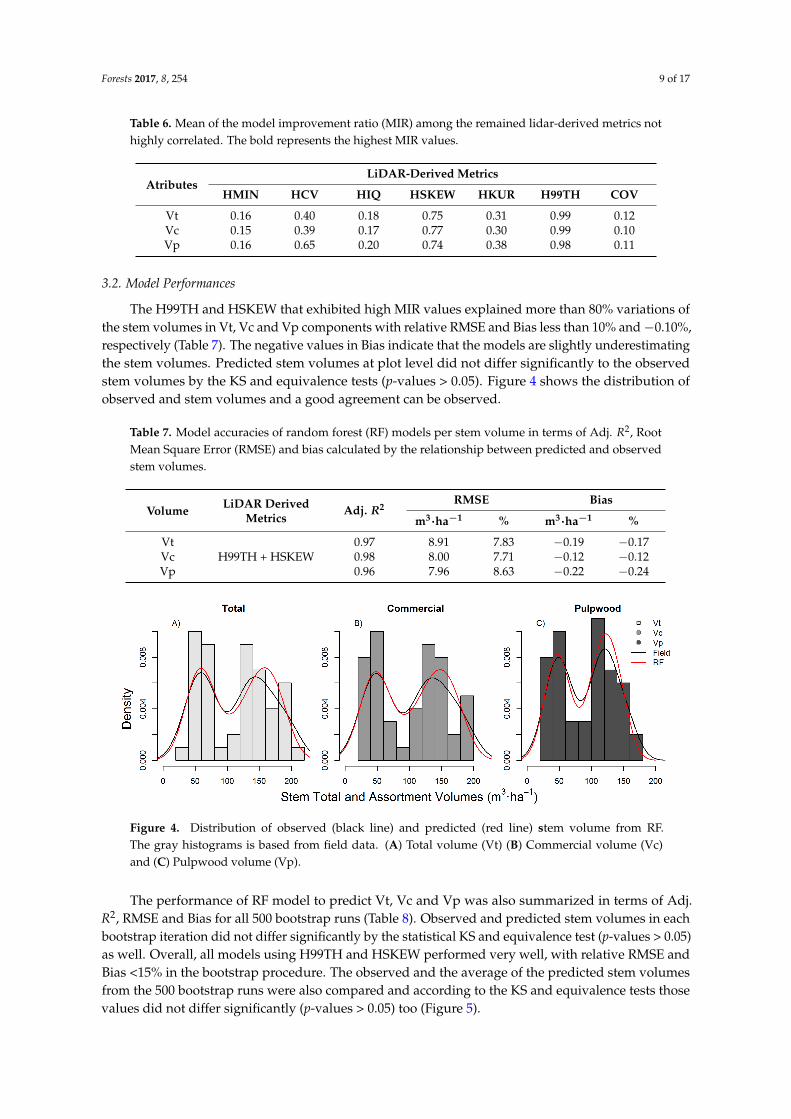
Table 6. Mean of the model improvement ratio (MIR) among the remained lidar-derived metrics nothighly correlated. The bold represents the highest MIR values.

AtributesLiDAR-Derived Metrics

HMIN HCV HIQ HSKEW HKUR H99TH COV

Vt 0.16 0.40 0.18 0.75 0.31 0.99 0.12Vc 0.15 0.39 0.17 0.77 0.30 0.99 0.10Vp 0.16 0.65 0.20 0.74 0.38 0.98 0.11

3.2. Model Performances

The H99TH and HSKEW that exhibited high MIR values explained more than 80% variations ofthe stem volumes in Vt, Vc and Vp components with relative RMSE and Bias less than 10% and −0.10%,respectively (Table 7). The negative values in Bias indicate that the models are slightly underestimatingthe stem volumes. Predicted stem volumes at plot level did not differ significantly to the observedstem volumes by the KS and equivalence tests (p-values > 0.05). Figure 4 shows the distribution ofobserved and stem volumes and a good agreement can be observed.

Table 7. Model accuracies of random forest (RF) models per stem volume in terms of Adj. R2, RootMean Square Error (RMSE) and bias calculated by the relationship between predicted and observedstem volumes.

Volume LiDAR DerivedMetrics

Adj. R2RMSE Bias

m3·ha−1 % m3·ha−1 %

Vt 0.97 8.91 7.83 −0.19 −0.17Vc H99TH + HSKEW 0.98 8.00 7.71 −0.12 −0.12Vp 0.96 7.96 8.63 −0.22 −0.24

Forests 2017, 8, 254 9 of 17

Table 6. Mean of the model improvement ratio (MIR) among the remained lidar-derived metrics not highly correlated. The bold represents the highest MIR values.

Atributes LiDAR-Derived Metrics

HMIN HCV HIQ HSKEW HKUR H99TH COV Vt 0.16 0.40 0.18 0.75 0.31 0.99 0.12 Vc 0.15 0.39 0.17 0.77 0.30 0.99 0.10 Vp 0.16 0.65 0.20 0.74 0.38 0.98 0.11

3.2. Model Performances

The H99TH and HSKEW that exhibited high MIR values explained more than 80% variations of the stem volumes in Vt, Vc and Vp components with relative RMSE and Bias less than 10% and −0.10%, respectively (Table 7). The negative values in Bias indicate that the models are slightly underestimating the stem volumes. Predicted stem volumes at plot level did not differ significantly to the observed stem volumes by the KS and equivalence tests (p-values > 0.05). Figure 4 shows the distribution of observed and stem volumes and a good agreement can be observed.

Table 7. Model accuracies of random forest (RF) models per stem volume in terms of Adj.R2, Root Mean Square Error (RMSE) and bias calculated by the relationship between predicted and observed stem volumes.

Volume LiDAR Derived

Metrics Adj. R2

RMSE Bias m3·ha−1 % m3·ha−1 %

Vt 0.97 8.91 7.83 −0.19 −0.17 Vc H99TH + HSKEW 0.98 8.00 7.71 −0.12 −0.12 Vp 0.96 7.96 8.63 −0.22 −0.24

Figure 4. Distribution of observed (black line) and predicted (red line) stem volume from RF. The gray histograms is based from field data. (A) Total volume (Vt) (B) Commercial volume (Vc) and (C) Pulpwood volume (Vp).

The performance of RF model to predict Vt, Vc and Vp was also summarized in terms of Adj. R2, RMSE and Bias for all 500 bootstrap runs (Table 8). Observed and predicted stem volumes in each bootstrap iteration did not differ significantly by the statistical KS and equivalence test (p-values > 0.05) as well. Overall, all models using H99TH and HSKEW performed very well, with relative RMSE and Bias <15% in the bootstrap procedure. The observed and the average of the predicted stem volumes from the 500 bootstrap runs were also compared and according to the KS and equivalence tests those values did not differ significantly (p-values > 0.05) too (Figure 5).

Figure 4. Distribution of observed (black line) and predicted (red line) stem volume from RF.The gray histograms is based from field data. (A) Total volume (Vt) (B) Commercial volume (Vc)and (C) Pulpwood volume (Vp).

The performance of RF model to predict Vt, Vc and Vp was also summarized in terms of Adj.R2, RMSE and Bias for all 500 bootstrap runs (Table 8). Observed and predicted stem volumes in eachbootstrap iteration did not differ significantly by the statistical KS and equivalence test (p-values > 0.05)as well. Overall, all models using H99TH and HSKEW performed very well, with relative RMSE andBias <15% in the bootstrap procedure. The observed and the average of the predicted stem volumesfrom the 500 bootstrap runs were also compared and according to the KS and equivalence tests thosevalues did not differ significantly (p-values > 0.05) too (Figure 5).

Forests 2017, 8, 254 10 of 17

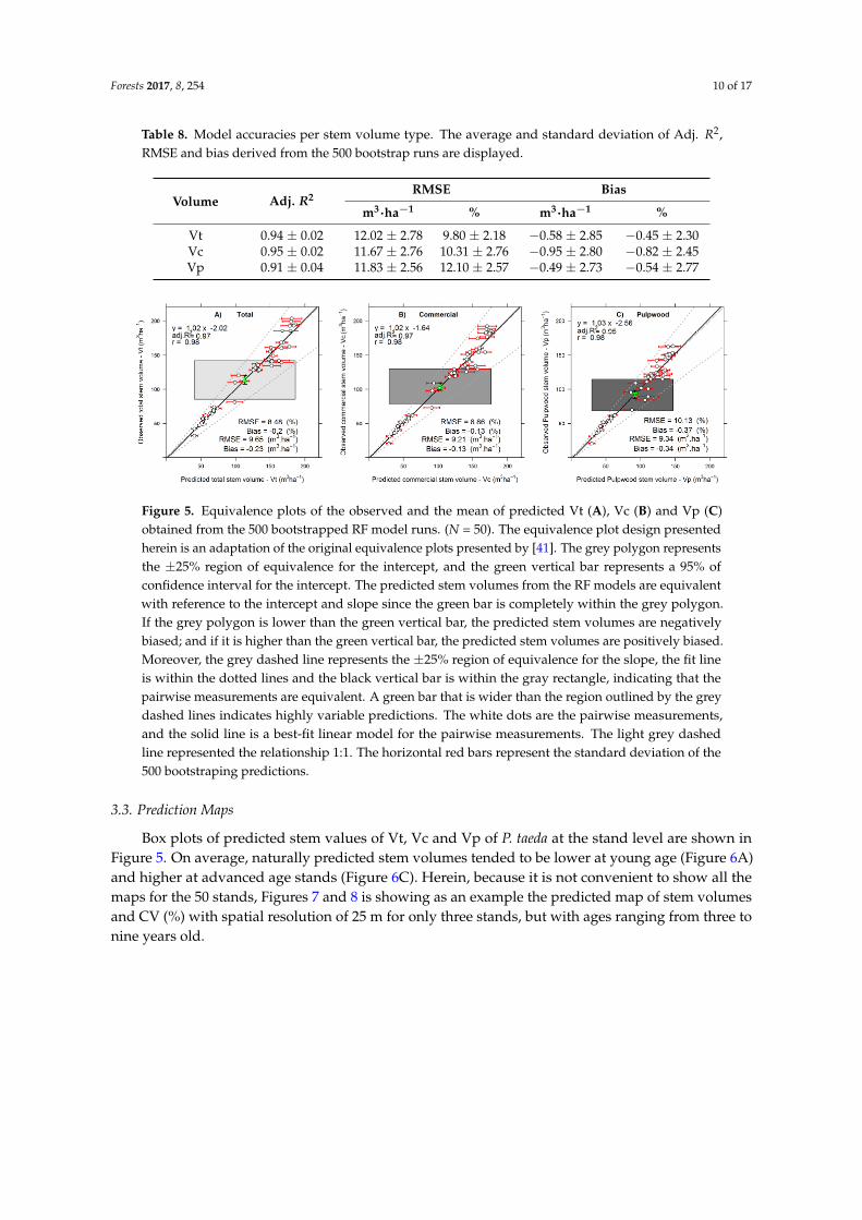
Table 8. Model accuracies per stem volume type. The average and standard deviation of Adj. R2,RMSE and bias derived from the 500 bootstrap runs are displayed.

Volume Adj. R2RMSE Bias

m3·ha−1 % m3·ha−1 %

Vt 0.94 ± 0.02 12.02 ± 2.78 9.80 ± 2.18 −0.58 ± 2.85 −0.45 ± 2.30Vc 0.95 ± 0.02 11.67 ± 2.76 10.31 ± 2.76 −0.95 ± 2.80 −0.82 ± 2.45Vp 0.91 ± 0.04 11.83 ± 2.56 12.10 ± 2.57 −0.49 ± 2.73 −0.54 ± 2.77

Forests 2017, 8, 254 10 of 17

Table 8. Model accuracies per stem volume type. The average and standard deviation of Adj. R2, RMSE and bias derived from the 500 bootstrap runs are displayed.

Volume Adj. R2 RMSE Bias

m3·ha−1 % m3·ha−1 % Vt 0.94 ± 0.02 12.02 ± 2.78 9.80 ± 2.18 −0.58 ± 2.85 −0.45 ± 2.30 Vc 0.95 ± 0.02 11.67 ± 2.76 10.31 ± 2.76 −0.95 ± 2.80 −0.82 ± 2.45 Vp 0.91 ± 0.04 11.83 ± 2.56 12.10 ± 2.57 −0.49 ± 2.73 −0.54 ± 2.77

Figure 5. Equivalence plots of the observed and the mean of predicted Vt (A), Vc (B) and Vp (C) obtained from the 500 bootstrapped RF model runs. (N = 50). The equivalence plot design presented herein is an adaptation of the original equivalence plots presented by [41]. The grey polygon represents the ±25% region of equivalence for the intercept, and the green vertical bar represents a 95% of confidence interval for the intercept. The predicted stem volumes from the RF models are equivalent with reference to the intercept and slope since the green bar is completely within the grey polygon. If the grey polygon is lower than the green vertical bar, the predicted stem volumes are negatively biased; and if it is higher than the green vertical bar, the predicted stem volumes are positively biased. Moreover, the grey dashed line represents the ±25% region of equivalence for the slope, the fit line is within the dotted lines and the black vertical bar is within the gray rectangle, indicating that the pairwise measurements are equivalent. A green bar that is wider than the region outlined by the grey dashed lines indicates highly variable predictions. The white dots are the pairwise measurements, and the solid line is a best-fit linear model for the pairwise measurements. The light grey dashed line represented the relationship 1:1. The horizontal red bars represent the standard deviation of the 500 bootstraping predictions.

3.3. Prediction Maps

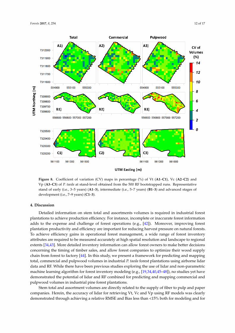
Box plots of predicted stem values of Vt, Vc and Vp of P. taeda at the stand level are shown in Figure 5. On average, naturally predicted stem volumes tended to be lower at young age (Figure 6A) and higher at advanced age stands (Figure 6C). Herein, because it is not convenient to show all the maps for the 50 stands, Figures 7 and 8 is showing as an example the predicted map of stem volumes and CV (%) with spatial resolution of 25 m for only three stands, but with ages ranging from three to nine years old.

Figure 5. Equivalence plots of the observed and the mean of predicted Vt (A), Vc (B) and Vp (C)obtained from the 500 bootstrapped RF model runs. (N = 50). The equivalence plot design presentedherein is an adaptation of the original equivalence plots presented by [41]. The grey polygon representsthe ±25% region of equivalence for the intercept, and the green vertical bar represents a 95% ofconfidence interval for the intercept. The predicted stem volumes from the RF models are equivalentwith reference to the intercept and slope since the green bar is completely within the grey polygon.If the grey polygon is lower than the green vertical bar, the predicted stem volumes are negativelybiased; and if it is higher than the green vertical bar, the predicted stem volumes are positively biased.Moreover, the grey dashed line represents the ±25% region of equivalence for the slope, the fit lineis within the dotted lines and the black vertical bar is within the gray rectangle, indicating that thepairwise measurements are equivalent. A green bar that is wider than the region outlined by the greydashed lines indicates highly variable predictions. The white dots are the pairwise measurements,and the solid line is a best-fit linear model for the pairwise measurements. The light grey dashedline represented the relationship 1:1. The horizontal red bars represent the standard deviation of the500 bootstraping predictions.

3.3. Prediction Maps

Box plots of predicted stem values of Vt, Vc and Vp of P. taeda at the stand level are shown inFigure 5. On average, naturally predicted stem volumes tended to be lower at young age (Figure 6A)and higher at advanced age stands (Figure 6C). Herein, because it is not convenient to show all themaps for the 50 stands, Figures 7 and 8 is showing as an example the predicted map of stem volumesand CV (%) with spatial resolution of 25 m for only three stands, but with ages ranging from three tonine years old.

Forests 2017, 8, 254 11 of 17

Forests 2017, 8, 254 11 of 17

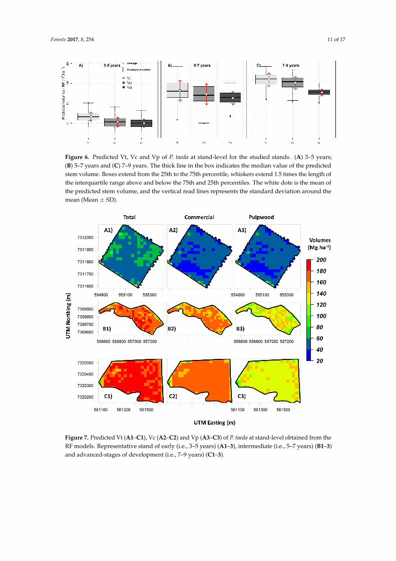
Figure 6. Predicted Vt, Vc and Vp of P. taeda at stand-level for the studied stands. (A) 3–5 years; (B) 5–7 years and (C) 7–9 years. The thick line in the box indicates the median value of the predicted stem volume. Boxes extend from the 25th to the 75th percentile, whiskers extend 1.5 times the length of the interquartile range above and below the 75th and 25th percentiles. The white dote is the mean of the predicted stem volume, and the vertical read lines represents the standard deviation around the mean (Mean ± SD).

Figure 7. Predicted Vt (A1–C1), Vc (A2–C2) and Vp (A3–C3) of P. taeda at stand-level obtained from the RF models. Representative stand of early (i.e., 3–5 years) (A1–3), intermediate (i.e., 5–7 years) (B1–3) and advanced-stages of development (i.e., 7–9 years) (C1–3).

Figure 6. Predicted Vt, Vc and Vp of P. taeda at stand-level for the studied stands. (A) 3–5 years;(B) 5–7 years and (C) 7–9 years. The thick line in the box indicates the median value of the predictedstem volume. Boxes extend from the 25th to the 75th percentile, whiskers extend 1.5 times the length ofthe interquartile range above and below the 75th and 25th percentiles. The white dote is the mean ofthe predicted stem volume, and the vertical read lines represents the standard deviation around themean (Mean ± SD).

Forests 2017, 8, 254 11 of 17

Figure 6. Predicted Vt, Vc and Vp of P. taeda at stand-level for the studied stands. (A) 3–5 years; (B) 5–7 years and (C) 7–9 years. The thick line in the box indicates the median value of the predicted stem volume. Boxes extend from the 25th to the 75th percentile, whiskers extend 1.5 times the length of the interquartile range above and below the 75th and 25th percentiles. The white dote is the mean of the predicted stem volume, and the vertical read lines represents the standard deviation around the mean (Mean ± SD).

Figure 7. Predicted Vt (A1–C1), Vc (A2–C2) and Vp (A3–C3) of P. taeda at stand-level obtained from the RF models. Representative stand of early (i.e., 3–5 years) (A1–3), intermediate (i.e., 5–7 years) (B1–3) and advanced-stages of development (i.e., 7–9 years) (C1–3).

Figure 7. Predicted Vt (A1–C1), Vc (A2–C2) and Vp (A3–C3) of P. taeda at stand-level obtained from theRF models. Representative stand of early (i.e., 3–5 years) (A1–3), intermediate (i.e., 5–7 years) (B1–3)and advanced-stages of development (i.e., 7–9 years) (C1–3).

Forests 2017, 8, 254 12 of 17

Forests 2017, 8, 254 12 of 17

Figure 8. Coefficient of variation (CV) maps in percentage (%) of Vt (A1–C1), Vc (A2–C2) and Vp (A3–C3) of P. taeda at stand-level obtained from the 500 RF bootstrapped runs. Representative stand of early (i.e., 3–5 years) (A1–3), intermediate (i.e., 5–7 years) (B1–3) and advanced stages of development (i.e., 7–9 years) (C1–3).

4. Discussion

Detailed information on stem total and assortments volumes is required in industrial forest plantations to achieve production efficiency. For instance, incomplete or inaccurate forest information adds to the expense and challenge of forest operations (e.g., [42]). Moreover, improving forest plantation productivity and efficiency are important for reducing harvest pressure on natural forests. To achieve efficiency gains in operational forest management, a wide range of forest inventory attributes are required to be measured accurately at high spatial resolution and landscape to regional extents [34,43]. More detailed inventory information can allow forest owners to make better decisions concerning the timing of timber sales, and allow forest companies to optimize their wood supply chain from forest to factory [44]. In this study, we present a framework for predicting and mapping total, commercial and pulpwood volumes in industrial P. taeda forest plantations using airborne lidar data and RF. While there have been previous studies exploring the use of lidar and non-parametric machine learning algorithm for forest inventory modeling (e.g., [19,34,40,45–48]), no studies yet have demonstrated the potential of lidar and RF combined for predicting and mapping commercial and pulpwood volumes in industrial pine forest plantations.

Stem total and assortment volumes are directly related to the supply of fiber to pulp and paper companies. Herein, the accuracy of lidar for retrieving Vt, Vc and Vp using RF models was clearly demonstrated through achieving a relative RMSE and Bias less than <15% both for modeling and for validation. As we are predicting forest attributes at a homogenous and single layered forest structure, our measures of precision and accuracy were similar to or higher than those who used lidar data for predicting stem volume through a RF framework in other forest types [15,16,42,44,49]. Among prior

Figure 8. Coefficient of variation (CV) maps in percentage (%) of Vt (A1–C1), Vc (A2–C2) andVp (A3–C3) of P. taeda at stand-level obtained from the 500 RF bootstrapped runs. Representativestand of early (i.e., 3–5 years) (A1–3), intermediate (i.e., 5–7 years) (B1–3) and advanced stages ofdevelopment (i.e., 7–9 years) (C1–3).

4. Discussion

Detailed information on stem total and assortments volumes is required in industrial forestplantations to achieve production efficiency. For instance, incomplete or inaccurate forest informationadds to the expense and challenge of forest operations (e.g., [42]). Moreover, improving forestplantation productivity and efficiency are important for reducing harvest pressure on natural forests.To achieve efficiency gains in operational forest management, a wide range of forest inventoryattributes are required to be measured accurately at high spatial resolution and landscape to regionalextents [34,43]. More detailed inventory information can allow forest owners to make better decisionsconcerning the timing of timber sales, and allow forest companies to optimize their wood supplychain from forest to factory [44]. In this study, we present a framework for predicting and mappingtotal, commercial and pulpwood volumes in industrial P. taeda forest plantations using airborne lidardata and RF. While there have been previous studies exploring the use of lidar and non-parametricmachine learning algorithm for forest inventory modeling (e.g., [19,34,40,45–48]), no studies yet havedemonstrated the potential of lidar and RF combined for predicting and mapping commercial andpulpwood volumes in industrial pine forest plantations.

Stem total and assortment volumes are directly related to the supply of fiber to pulp and papercompanies. Herein, the accuracy of lidar for retrieving Vt, Vc and Vp using RF models was clearlydemonstrated through achieving a relative RMSE and Bias less than <15% both for modeling and for

Forests 2017, 8, 254 13 of 17

validation. As we are predicting forest attributes at a homogenous and single layered forest structure,our measures of precision and accuracy were similar to or higher than those who used lidar datafor predicting stem volume through a RF framework in other forest types [15,16,42,44,49]. Amongprior studies, RF has generally showed better performance compared to other statistical approaches,such as multiple linear regression, boosting trees regression and support vector regression [50–53].Lidar-derived stem total and saw log volumes and their estimation accuracies have previously beenreported at the forest stand level (e.g., [15,16,42,54,55]). For instance, in Eastern Finland in a typicalFinnish southern boreal managed forest area, two studies used lidar data for estimating species-specificdiameter distributions and saw log volumes [15,16]. Two years later, in Southern Wisconsin, USA, lidardata were used for predicting not only saw log volume, but also pulpwood volume [55]; the modelsproduced R2 of ~0.65 for estimating both saw log and pulpwood volumes. While those authors haveshowed the great potential of lidar in retrieving assortment volumes, this specific application is stillrelatively novel and further studies, such as presented herein, still need to be carried out.

In this study, we showed that lidar measurements could be used as input data to predict andmap stem total and assortment volumes through a RF framework. High levels of accuracy were foundwhen predicting Vt, Vc and Vp volumes across variable stand ages of P. taeda using only H99TH andHSKEW as predictor variables. Lidar-derived H99TH represents the top of the canopy (height at 99thpercentile) and HSKEW is a measure of the asymmetry of height distribution, which is associated withthe age of the stands because older trees are taller and cause a more positively skewed distribution.Skewness and height percentile variables are logical selections for distinguishing between differentvolume levels based on distributional shapes and height frequencies [56]. In particular, these variablescan explain changes in the volume distribution [5], thus providing a solid justification for inclusion inthe predictive model. Our results suggest that models based on variables describing the height of thecanopy and the symmetry of the distribution of the returns are capable of predicting stem total andassortment volumes across different tree ages in industrial P. taeda forest plantations. Height percentilelidar metrics, such as H99TH, and height distributional metrics, such as HSKEW, have been shown tobe powerful metrics for modeling and predicting forest attributes (e.g., [5–7,33,34,48]).

A disadvantage of using the RF framework presented here is that RF models do not extrapolatepredictions beyond the trained data, and consequently, as found herein, reduce the variance comparedto the observations (Figure 5). However, an important advantage of non-parametric approaches,such as RF, is that they can model non-linear, complex relationships between the dependent and theindependent variables more efficiently than parametric approaches [46]. Furthermore, RF is insensitiveto data skew, robust to a high number of variable inputs, and its implementation does not requirepre-stratification by forest type [20,34,46]. From an overall statistical perspective, the predicted andobserved volumes were equivalent, although our RF model validations showed a systematic tendencyto overestimate small values and underestimate high values. The same was found in previous studies(e.g., [40,57]). According to one study [57], a possible cause might be that because the RF model estimatesvalues by averaging the predictions of many decision trees, it might tend to underestimate when thepredicted value is close to the maximum value of the training data. Similarly, when the estimated valueis close to the minimum value of training data it might tend to overestimate. Other possible causes mightbe that we have a relatively small number of field plots, especially in the young and older stands.

Traditional forest inventory approaches are not effective in terms of costing and mobility especiallyin P. taeda forest plantations, where there is a need to monitor annual forest growth and properties arevery large. Lidar remote sensing constitutes an important step towards operational wood procurementplanning and is of high current interest to forestry organizations. Such technology is of great interestowing to their spatial sampling capabilities within plantations, and have had great reliability inforest inventory work in countries such as Norway, Canada, or the USA (e.g., [6,7,12,58]). Moreover,the application of airborne lidar technology for Brazilian industrial management is relatively new.While some studies have showed that the cost of the forest inventory derived from lidar could belower than conventional forest inventory [59,60], the cost of lidar data acquisition could still be high

Forests 2017, 8, 254 14 of 17

to monitor forest growth annually; however, lidar has the ability to provide wall-to-wall, accuratemapping of forest attributes at high spatial resolutions (e.g., Figures 7 and 8).

Traditional forest inventory approaches are based on sampling theory, and forest attributesmeasured at plot level are then used to infer inventory attributes for an entire stand [5,14]. We showedhere that lidar and RF machine learning combined can be a powerful tool for mapping forest attributesin P. taeda forest plantations. In practice, lidar-derived maps of stem total and assortment volumes(Figures 7 and 8) allow the owners to evaluate the production and forest structure variability withinstands in a spatially explicit manner, which is not possible in a traditional forest inventory of P. taeda.Also, such maps may allow managers to detect spatial patterns related to tree diseases, fire orforest clearing.

Recently, a study carried out in Eucalyptus spp. forest plantations showed that lidar and RFcould be combined to predict and map aboveground carbon at high spatial resolution (5 m), even ifthe models are calibrated using field plots with area larger than the cell size used for mapping [34].Therefore, future studies should be also test the ability of lidar and RF to map stem total and assortmentvolumes even at higher spatial resolution than presented in this study (e.g., Figures 7 and 8). Herein, wedemonstrated the potential of combined lidar-derive metrics and RF to predict forest attributes througha lidar-plot based approach framework, however, to get even higher amount of details in P. taeda forestplantations, RF could be also tested in a lidar-individual tree based approach. For instance, RF hasbeen successfully used to impute individual tree height and volume in longleaf pine (Pinus palustrisMill.) forest in Southern USA [61]; therefore, lidar and RF could be also used to predict stem total andassortment volumes at an individual tree level in P. taeda forest plantations, if carefully implemented.

5. Conclusions

Refining strategies for improving productivity of forest plantations requires accurate and detailedspatial information on forest structure and growing stock volume. In this study, we showed thatairborne lidar data metrics can predict total, commercial and pulpwood volumes in a P. taeda forestplantation in Brazil. We found that different stem volumes can be estimated with high levels of accuracyfrom two lidar-derived variables describing the height and the shape of the vertical distribution ofthe height. The use of a model based on two variables suggests a higher generalization potential thanmodels based on specific metrics that could result in over-fitting. However, this potential should betested in other plantations and forested environments. Although airborne lidar data has not beenadopted by paper companies operationally, our results show that the method used could be readilyapplied to support the supply chain of pulp and paper companies in Brazil or elsewhere.

Acknowledgments: This research was funded through a PhD scholarship from the National Councilof Technological and Scientific Development (CNPq) via the Science without Borders Program (Process249802/2013-9) and USDA Forest Service. The authors are very grateful for the lidar and field inventory datacollections funded by Klabin S.A., a pulp and paper company. Mariano Garcia is supported by a Marie CurieInternational Outgoing Fellowship within the 7th European Community Framework Programme (ForeStMap—3DForest Structure Monitoring and Mapping, Project Reference: 629376). The contents on this paper reflect only theauthors’ views and not the views of the European Commission. We thank three anonymous reviewers for theirhelpful suggestions on the first version of the manuscript.

Author Contributions: All the authors have made substantial contribution towards the successful completionof this manuscript. They all have been involved in designing the study, drafting the manuscript and engagingin critical discussion. C.A.S., C.K., A.T.H., L.A.V., W.S.W.M.J. and M.M., contributed with the methodologicalframework, data processing analysis and write up. M.G., A.F., A.C. and S.S. contributed to the interpretation,quality control and revisions of the manuscript. All authors read and approved the final manuscript.

Conflicts of Interest: The authors declare no conflict of interest.

References

1. Payn, T.; Carnus, J.-M.; Freer-Smith, P.; Kimberley, M.; Kollert, W.; Liu, S.; Orazio, C.; Rodriguez, L.;Silva, L.N.; Wingfield, M.J. Changes in planted forests and future global implications. For. Ecol. Manag. 2015,352, 57–67. [CrossRef]

Forests 2017, 8, 254 15 of 17

2. Indústria Brasileira de Árvores (IBÁ). Brazilian Tree Industry. 2015. Available online: http://www.iba.org/images/shared/iba_2015.pdf (accessed on 10 November 2016).

3. Kohler, S.V.; Wolff, N.I.; Figueiredo Filho, A.; Arce, J.E. Dynamic of assortment of Pinus taeda L. plantation indifferent site classes in Southern Brazil. Sci. For. 2014, 42, 403–410.

4. Silva, C.A.; Klauberg, C.; Hudak, A.T.; Vierling, L.A.; Liesenberg, V.; Bernett, L.G.; Scheraiber, C.F.;Schoeninger, E.R. Estimating Stand Height and Tree Density in Pinus taeda plantations using in-situ data,airborne LiDAR and k-Nearest Neighbor Ismputation. Ann. Braz. Acad. Sci. 2017, 90, 1–15, in press.

5. Silva, C.A.; Klauberg, C.; Hudak, A.T.; Vierling, L.A.; Liesenberg, V.; Carvalho, S.P.; Rodriguez, L.C.A principal component approach for predicting the stem volume in Eucalyptus plantations in Brazil usingairborne Lidar data. Forestry 2016, 89, 422–433. [CrossRef]

6. Næsset, E. Determination of mean tree height of forest stands using airborne laser scanner data. ISPRS J.Photogramm. 1997, 52, 49–56. [CrossRef]

7. Næsset, E. Predicting forest stand characteristics with airborne scanning laser using a practical two-stageprocedure and field data. Remote Sens. Environ. 2002, 80, 88–99. [CrossRef]

8. Næsset, E.; Gobakken, T.; Holmgren, J.; Hyyppä, H.; Hyyppä, J.; Maltamo, M.; Nilsson, M.; Olsson, H.;Persson, Å.; Söderman, U. Laser scanning of forest resources: The Nordic experience. Scand. J. For. Res. 2004,19, 482–499. [CrossRef]

9. Næsset, E. Airborne laser scanning as a method in operational forest inventory: Status of accuracyassessments accomplished in Scandinavia. Scand. J. For. Res. 2007, 22, 433–442. [CrossRef]

10. Hudak, A.T.; Evans, J.S.; Stuart, A.M. Lidar utility for natural resource managers. Remote Sens. 2009, 1,934–951. [CrossRef]

11. Andersen, H.E.; McGaughey, R.J.; Reutebuch, S.E. Estimating forest canopy fuel parameters using lidar data.Remote Sens. Environ. 2005, 94, 441–449. [CrossRef]

12. Hudak, A.T.; Crookston, N.L.; Evans, J.S.; Falkowski, M.J.; Smith, A.M.; Gessler, P.E.; Morgan, P. Regressionmodeling and mapping of coniferous forest basal area and tree density from discrete-return lidar andmultispectral satellite data. Can. J. Remote Sens. 2006, 32, 126–138. [CrossRef]

13. White, J.C.; Wulder, M.A.; Buckmaster, G. Validating estimates of merchantable volume from airborne laserscanning (ALS) data using weight scaled data. For. Chron. 2014, 90, 378–385. [CrossRef]

14. Silva, C.A.; Klauberg, C.; Carvalho, S.D.P.C.; Hudak, A.T. Mapping aboveground carbon stocks using Liardata in Eucalyptus spp. plantations in the state of São Paulo, Brazil. Sci. For. 2014, 42, 591–604.

15. Korhonen, L.; Peuhkurinen, J.; Jukka, M.; Suvanto, A.; Maltamo, M.; Packalen, P.; Kangas, J. The use ofairborne laser scanning to estimate sawlog volumes. Forestry 2008, 81, 499–510. [CrossRef]

16. Peuhkurinen, J.; Maltamo, M.; Malinen, J. Estimating Species-Specific diameter distributions and saw logrecoveries of boreal forests from airborne laser scanning data and aerial photographs: A distribution-basedapproach. Silva Fenn. 2008, 42, 600–625. [CrossRef]

17. Sherrill, J.R.; Bullock, B.P.; Mullin, T.J.; McKeand, S.E.; Purnell, R.C. Total and merchantable stem volumeequations for mid rotation loblolly pine (Pinus taeda L.). South. J. Appl. For. 2011, 35, 105–108.

18. Hudak, A.T.; Crookston, N.L.; Evans, J.S.; Hall, D.E.; Falkowski, M.J. Nearest neighbor imputation ofspecies-level, plot-scale forest structure attributes from lidar data. Remote Sens. Environ. 2008, 112, 2232–2245.[CrossRef]

19. Ahmed, O.S.; Franklin, S.E.; Wulder, M.A.; White, J.C. Characterizing stand-level forest canopy cover andheight using landsat time series, samples of airborne lidar, and the random forest algorithm. ISPRS J.Photogramm. Remote Sens. 2015, 101, 89–101. [CrossRef]

20. Breiman, L. Random forests. Mach. Learn. 2001, 45, 5–32. [CrossRef]21. Grossmann, E.; Ohmann, J.; Kagan, J.; May, H.; Gregory, M. Mapping ecological systems with a random

forest model: Tradeoffs between errors and bias. GAP Anal. Bull. 2010, 17, 16–22.22. Naidoo, L.; Cho, M.A.; Mathieu, R.; Asner, G. Classification of savanna tree species, in the Greater Kruger

National Park region, by integrating hyperspectral and Lidar data in a Random Forest data miningenvironment. ISPRS J. Photogramm. Remote Sens. 2012, 69, 167–179. [CrossRef]

23. Yu, X.; Hyyppä, J.; Vastaranta, M.; Holopainen, M.; Viitala, R. Predicting individual tree attributes fromairborne laser point clouds based on the random forests technique. ISPRS J. Photogramm. Remote Sens. 2011,661, 28–37. [CrossRef]

Forests 2017, 8, 254 16 of 17

24. Ko, C.; Sohn, G.; Remmel, T.K.; Miller, J.R. Maximizing the Diversity of Ensemble Random Forests for TreeGenera Classification Using High Density Lidar Data. Remote Sens. 2016, 8, 646. [CrossRef]

25. Olden, J.D.; Lawler, J.J.; Poff, N.L. Machine learning methods without tears: A primer for ecologists.Q. Rev. Biol. 2008, 83, 171–193. [CrossRef] [PubMed]

26. Stumpf, A.; Kerle, N. Object-oriented mapping of landslides using Random Forests. Remote Sens. Environ.2011, 115, 2564–2577. [CrossRef]

27. Lawrence, R.L.; Wood, S.D.; Sheley, R.L. Mapping invasive plants using hyperspectral imagery and BreimanCutler classifications (RandomForest). Remote Sens. Environ. 2006, 100, 356–362. [CrossRef]

28. Köppen, W.; Geiger, R. Klimakarte der Erde. Wall-Map 150 cm × 200 cm; Verlag Justus Perthes: Gotha, Germany, 1928.29. Curtis, R.O. Height-diameter and height-diameter-age equations for second-growth Douglas-fir. For. Sci.

1967, 13, 365–375.30. Schöpfer, W. Automatisierung Des Massem, Sorten Und Wertberechnung Stenender Waldbestande Schriftenreihe

Bad; Wurtt-Forstl: Koblenz, Germany, 1966.31. McGauchey, R.J. FUSION/LDV: Software for LiDAR Data Analysis and Visualization; Forest Service Pacific

Northwest Research Station USDA: Seattle, WA, USA, 2015. Available online: http://forsys.cfr.washington.edu/fusion/FUSIONmanual.pdf (accessed on 15 October 2015).

32. Kraus, K.; Pfeifer, N. Determination of terrain models in wooded areas with airborne laser scanner data.ISPRS J. Photogramm. Remote Sens. 1998, 53, 193–203. [CrossRef]

33. Hudak, A.T.; Strand, E.K.; Vierling, L.A.; Byrne, J.C.; Eitel, J.U.H.; Martinuzzi, S.; Falkowski, M.J. Quantifyingaboveground forest carbon pools and fluxes from repeat LiDAR surveys. Remote Sens. Environ. 2012, 123,25–40. [CrossRef]

34. Silva, C.A.; Hudak, A.T.; Klauberg, C.; Vierling, L.A.; Gonzalez-Benecke, C.; de Padua Chaves Carvalho, S.;Rodriguez, L.C.E.; Cardil, A. Combined effect of pulse density and grid cell size on predicting andmapping aboveground carbon in fast-growing Eucalyptus forest plantation using airborne LiDAR data.Carbon Balance Manag. 2017, 12, 13. [CrossRef] [PubMed]

35. Evans, J.S.; Cushman, S.A. Gradient modeling of conifer species using Random Forests. Landsc. Ecol. 2009, 5,673–683. [CrossRef]

36. Evans, J.S.; Murphy, M.A.; Holden, Z.A.; Cushman, S.A. Modeling species distribution and change usingRandom Forests. In Predictive Modeling in Landscape Ecology; Drew, C.A., Huettmann, F., Wiersma, Y., Eds.;Springer: New York, NY, USA, 2010; pp. 139–159.

37. Liaw, A.; Wiener, M. RandomForest: Breiman and Cutler’s Random Forests for Classification and Regression,Version 4.6–12. 2015. Available online: https://cran.rproject.org/web/packages/randomForest/ (accessedon 15 October 2016).

38. R Core Team. R: A Language and Environment for Statistical Computing; R Foundation for Statistical Computing:Vienna, Austria, 2017. Available online: http://www.R-project.org (accessed on 20 October 2016).

39. Bright, B.C.; Hudak, A.T.; McGaughey, R.; Andersen, H.E.; Negron, J. Predicting live and dead tree basal areaof bark beetle affected forests from discrete-return lidar. Can. J. Remote Sens. 2013, 39, S99–S111. [CrossRef]

40. Lopatin, J.; Dolos, K.; Hernández, H.J.; Galleguillos, M.; Fassnacht, F.E. Comparing Generalized LinearModels and random forest to model vascular plant species richness using LiDAR data in a natural forest incentral Chile. Remote Sens. Environ. 2016, 173, 200–210. [CrossRef]

41. Robinson, A.P.; Duursma, R.A.; Marshall, J.D. A regression-based equivalence test for model validation:Shifting the burden of proof. Tree Physiol. 2005, 25, 903–913. [CrossRef] [PubMed]

42. Holopainen, M.; Vastaranta, M.; Rasinmäki, J.; Kalliovirta, J.; Mäkinen, A.; Haapanen, R.; Melkas, T.; Yu, X.;Hyyppä, J. Uncertainty in timber assortment estimates predicted from forest inventory data. Eur. J. For. Res.2010, 129, 1131–1142. [CrossRef]

43. Sibona, E.; Vitali, A.; Meloni, F.; Caffo, L.; Dotta, A.; Lingua, E.; Motta, R.; Garbarino, M. Direct Measurementof Tree Height Provides Different Results on the Assessment of LiDAR Accuracy. Forests 2017, 8, 7. [CrossRef]

44. Kankare, V.; Vauhkonen, J.; Tanhuanpaa, T.; Holopainen, M.; Vastaranta, M.; Joensuu, M. Accuracy inestimation of timber assortments and stem distribution—A comparison of airborne and terrestrial laserscanning techniques. ISPRS J. Photogramm. Remote Sens. 2014, 97, 89–97. [CrossRef]

45. Zhao, K.; Popescu, S.; Meng, X.; Pang, Y.; Agca, M. Characterizing forest canopy structure with lidarcomposite metrics and machine learning. Remote Sens Environ. 2011, 115, 1978–1996. [CrossRef]

Forests 2017, 8, 254 17 of 17

46. Mascaro, J.; Asner, G.P.; Knapp, D.E.; Kennedy-Bowdoin, T.; Martin, R.E.; Anderson, C.; Higgins, M.;Chadwick, K.D. A tale of two “forests”: Random forest machine learning AIDS tropical forest carbonmapping. PLoS ONE 2014, 9, e85993. [CrossRef] [PubMed]

47. García Gutiérrez, J.; Martínez Álvarez, F.; Troncoso Lora, A.; Riquelme Santos, J.C. A comparison of machinelearning regression techniques for LiDAR-derived estimation of forest variables. Neurocomputing 2015, 167,24–31. [CrossRef]

48. Hudak, A.T.; Bright, B.C.; Pokswinski, S.M.; Loudermilk, E.L.; O’Brien, J.J.; Hornsby, B.S.; Klauberg, C.;Silva, C.A. Mapping forest structure and composition from low-density LiDAR for informed forest, fuel, andfire management at Eglin Air Force Base, Florida, USA. Can. J. Remote Sens. 2016, 42, 411–427. [CrossRef]

49. Hayashi, R.; Weiskittel, A.; Sader, S. Assessing the feasibility of low-density lidar for stand inventory attributepredictions in complex and managed forests of Northern Maine, USA. Forests 2014, 5, 363–383. [CrossRef]

50. Kankare, V.; Vastaranta, M.; Holopainen, M.; Raty, M.; Yu, X.; Hyyppa, J.; Hyyppa, H.; Alho, P.; Viitala, R.Retrieval of forest aboveground biomass and stem volume with airborne scanning LiDAR. Remote Sens. 2013,5, 2257–2274. [CrossRef]

51. Wu, J.; Yao, W.; Choi, S.; Park, T.; Myneni, R.B. A Comparative Study of Predicting DBH and Stem Volume ofIndividual Trees in a Temperate Forest Using Airborne Waveform LiDAR. IEEE Geosci. Remote Sens. Lett.2015, 12, 2267–2271. [CrossRef]

52. Shataeea, S.; Weinaker, H.; Babanejad, M. Plot-level Forest Volume Estimation Using Airborne Laser Scannerand TM Data, Comparison of Boosting and Random Forest Tree Regression Algorithms. Procedia Environ. Sci.2011, 7, 68–73. [CrossRef]

53. Peuhkurinen, J.; Maltamo, M.; Malinen, J.; Pitkänen, J.; Packalén, P. Pre-harvest measurement of markedstands using airborne laser scanning. For. Sci. 2007, 53, 653–661.

54. Holmgren, J.; Barth, A.; Larsson, H.; Olsson, H. Prediction of stem attributes by combining airborne laserscanning and measurements from harvesters. Silva Fen. 2012, 46, 227–239. [CrossRef]

55. Hawbaker, T.J.; Gobakken, T.; Lesak, A.; Trømborg, E.; Contrucci, K.; Radeloff, V. Light detection andranging-based measures of mixed hardwood forest structure. For. Sci. 2010, 56, 313–326.

56. Van Aardt, J.A.N.; Wynne, R.H.; Oderwald, R.G. Forest Volume and Biomass Estimation UsingSmall-Footprint Lidar Distributional Parameters on a Per-Segment Basis. For. Sci. 2006, 52, 636–649.

57. Ota, T.; Ahmed, O.S.; Franklin, S.E.; Wulder, M.A.; Kajisa, T.; Mizoue, N. Estimation of Airborne LidarDerived Tropical Forest Canopy Height Using Landsat Time Series in Cambodia. Remote Sens. 2014, 6,10750–10772. [CrossRef]

58. Coops, N.C.; Hilker, T.; Wulder, M.A.; St-Onge, B.; Newnham, G.; Siggins, A. Estimating canopy structure ofDouglas-fir forest stands from discrete-return lidar. Trees 2007, 21, 295–310. [CrossRef]

59. Tilley, B.K.; Munn, I.A.; Evans, D.L.; Parker, R.C.; Roberts, S.D. Cost Considerations of Using Lidar forTimber Inventory. 2004. Available online: http://sofew.cfr.msstate.edu/papers/0504tilley.pdf/ (accessed on21 March 2016).

60. Hummel, S.; Hudak, A.T.; Uebler, E.H.; Falkowski, M.J.; Megown, K.A. A comparison of accuracy and costof LiDAR versus stand exam data for landscape management on the Malheur national forest. J. For. 2011,109, 267–273.

61. Silva, C.A.; Hudak, A.T.; Vierling, L.A.; Loudermilk, E.L.; O’Brien, J.J.; Hiers, J.K.; Jack, S.B.;Gonzalez-Benecke, C.A.; Lee, H.; Falkowski, M.J.; et al. Imputation of individual longleaf pine forestattributes from field and LiDAR data. Can. J. Remote Sens. 2016, 42, 554–573. [CrossRef]

© 2017 by the authors. Licensee MDPI, Basel, Switzerland. This article is an open accessarticle distributed under the terms and conditions of the Creative Commons Attribution(CC BY) license (http://creativecommons.org/licenses/by/4.0/).