Page 1
Predicting Student Retention and Academic Success at NewMexico Tech
by
Julie Luna
Submitted in Partial Fulfillment
of the Requirements for the Degree of
Master of Science in Mathematics
with Operations Research and Statistics Option
New Mexico Institute of Mining and Technology
Socorro, New Mexico
August, 2000
Page 2
ii
ACKNOWLEGEMENT
The data set for this study was provided by Luz Barreras, Registrar at the New
Mexico Institute of Mining and Technology. Joe Franklin of the Information Services
Department made the necessary preparations for me to access the database.
In the beginning stages of this study, Allan Gutjahr helped to form the underlying
structure of this thesis. I was very privileged to have been able to work with him.
I owe many thanks to my advisor, Brian Borchers, and to my committee
members, Bill Stone and Emily Nye for their guidance and support on this thesis. I also
need to thank the Mathematics Department for their constant encouragement.
Page 3
iii
Abstract
Focusing on new, incoming freshmen, this study examines several variables to see
which can provide information about retention and academic outcome after three
semesters. Two parametric classification models and one non-parametric classification
model were used to predict various outcomes based upon persistence and academic
standing. These classification models were: Logistic Regression, Discriminant Analysis,
and Classification and Regression Trees (CART). In addition, the outcome of the
freshmen who participated in the Group Opportunities for Activities and Learning
(GOAL) program were examined to determine if these students were retained and
performed well academically at higher rates than predicted given their admission criteria.
Page 4
iv
Table of Contents
Acknowledgement ii
Abstract iii
Table of Contents iv
List of Tables vi
List of Figures viii
1. Introduction
1.1 Background ………………………………………………………………… 1
1.2 Description of Classification Models ……………………………………… 5
1.3 Three Different Classification Models ……………………………………. 8
1.4 Previous Studies …………………………………………………………… 11
2. Data Collection and Preliminary Analysis ……………………………………... 15
3. Methods used to Construct the Classification Model
3.1 Logistic Regression ………………………………………………………... 31
3.2 CART ……………………………………………………………………… 36
3.3 Discriminant Analysis ……………………………………………………… 38
4. Results
4.1 Prediction of Fall to Fall Persistence
4.1.1 Logistic Regression …………………………………………….. 45
4.1.2 CART …………………………………………………………… 47
4.1.3 Discriminant Analysis …………………………………………... 49
4.2 Prediction of Fall to Fall Persistence with Good Academic Standing
4.2.1 Logistic Regression ……………………………………………… 51
4.2.2 CART …………………………………………………………. 61
4.2.3 Discriminant Analysis ………………………………………… 71
4.3 Prediction of Academic Success …………………………………………. 75
4.3.1 Logistic Regression …………………………………………… 77
Page 5
v
4.3.2 CART ………………………………………………………….. 84
4.3.3 Discriminant Analysis …………………………………………. 89
5. GOAL Program ………………………………………………………………… 95
6. Conclusions ……………………………………………………………………… 99
References …………………………………………………………………………... 108
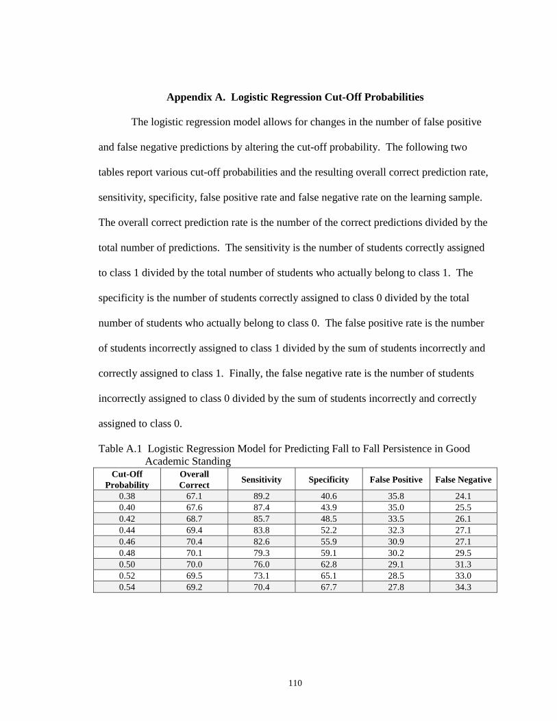
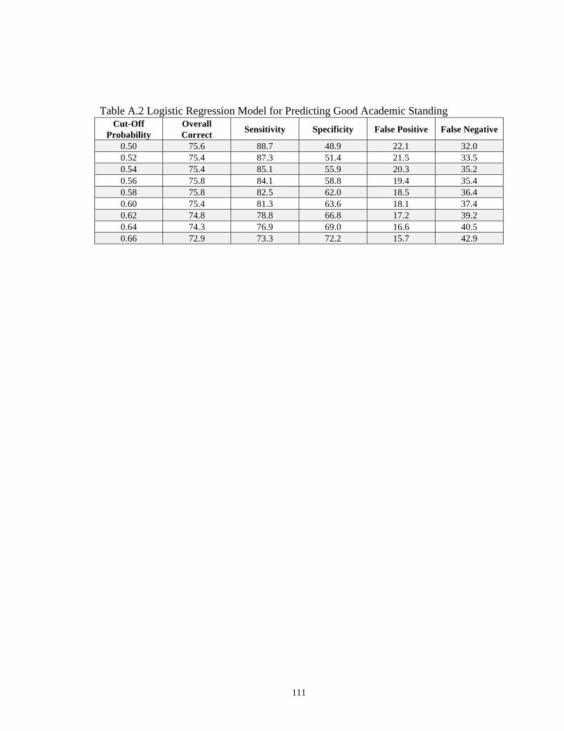
A. Logistic Regression Cut-Off Probabilities …………………………………….. 110
B. Results Using a Reduced Data Set from Raising the Minimum High School Grade Point Average …………………………………………………………… 112
Page 6
vi
List of Tables
2.1 Student Database Tables ……………………………………………………... 15
2.2 Variable Information …………………………………………………………. 17
2.3 ACT Exam Content …………………………………………………………… 26
3.1 DA Test Models ………………………………………………………….…… 44
4.1 LR Univariate Analysis (First Outcome) …………………………………….. 45
4.2 CART Tree Prediction Rates (First Outcome) ……………………………….. 48
4.3 DA Test Models (First Outcome) ……………………………………………. 50
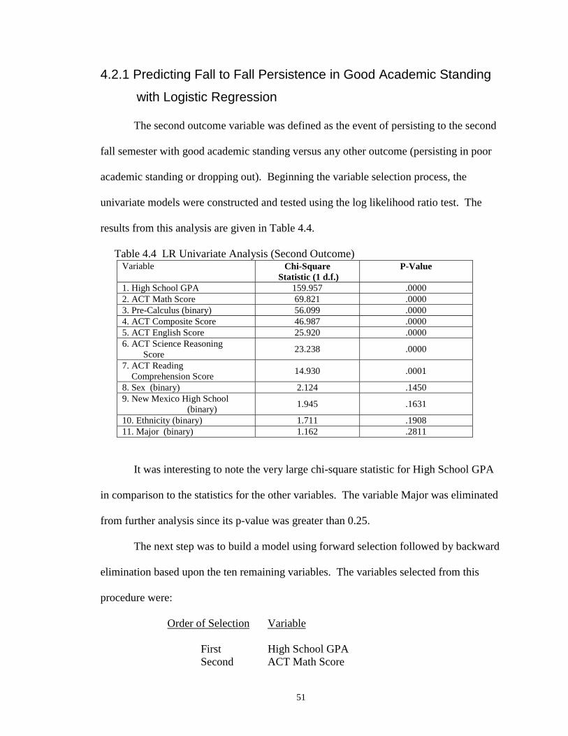
4.4 LR Univariate Analysis (Second Outcome) ………………………………….. 51
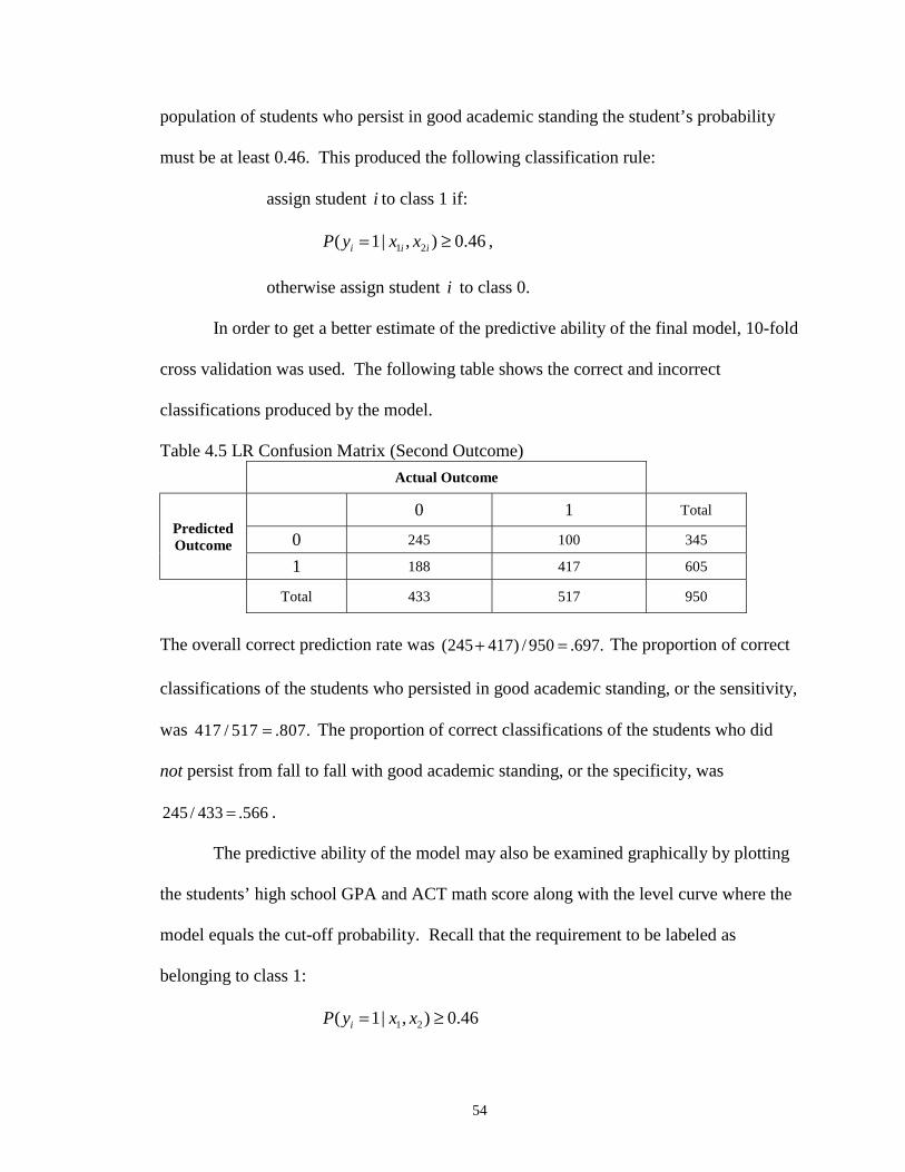
4.5 LR Confusion Matrix (Second Outcome) ……………………………….…… 54
4.6 CART Tree Prediction Rates (Second Outcome) ……………………………. 62
4.7 CART Confusion Matrix (Second Outcome) …………………………….….. 66
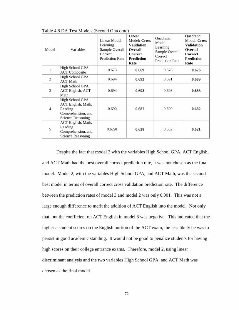
4.8 DA Test Models (Second Outcome) ………………………………………… 72
4.9 DA Confusion Matrix (Second Outcome) …………………………………… 73
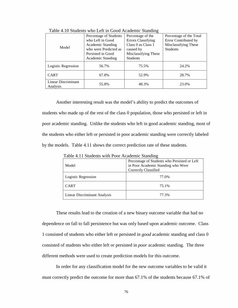
4.10 Students who Left in Good Academic Standing ………………………….…. 76
4.11 Students with Poor Academic Standing ……………………………………... 76
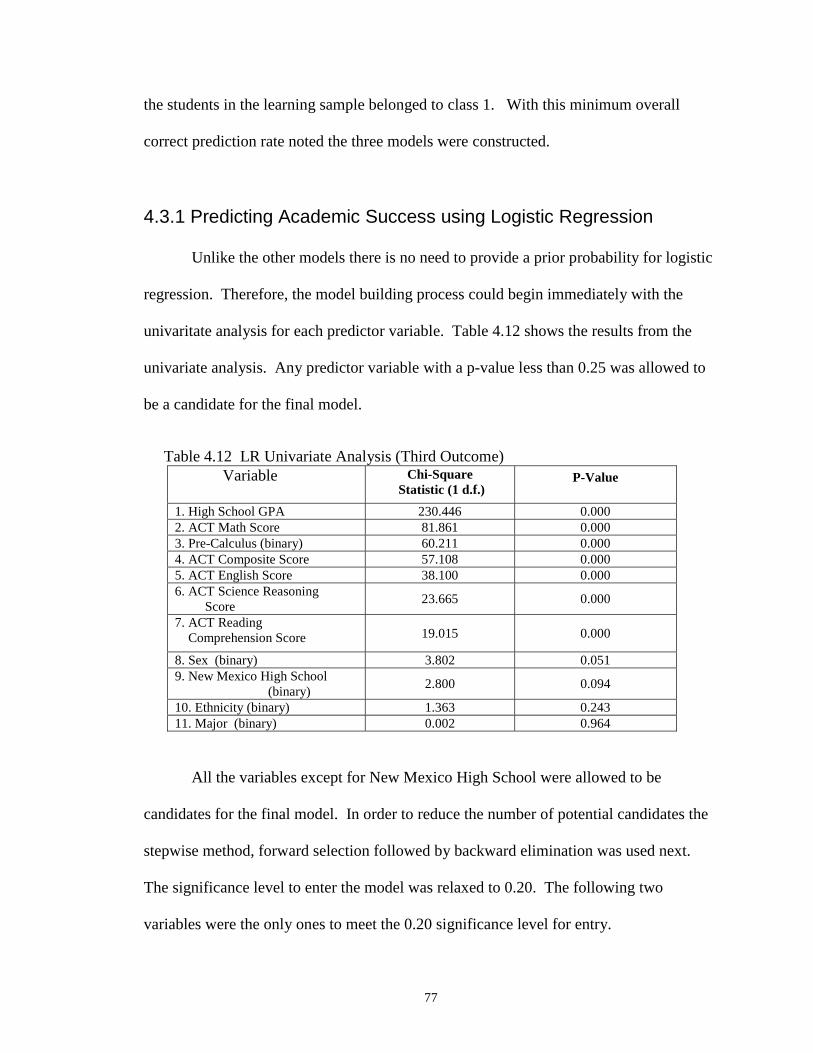
4.12 LR Univariate Analysis (Third Outcome) …………………………………… 77
4.13 LR Confusion Matrix (Third Outcome) ……………………………………... 78
4.14 CART Tree Prediction Rates (Third Outcome) ……………………………… 85
4.15 CART Confusion Matrix (Third Outcome) ………………………………….. 87
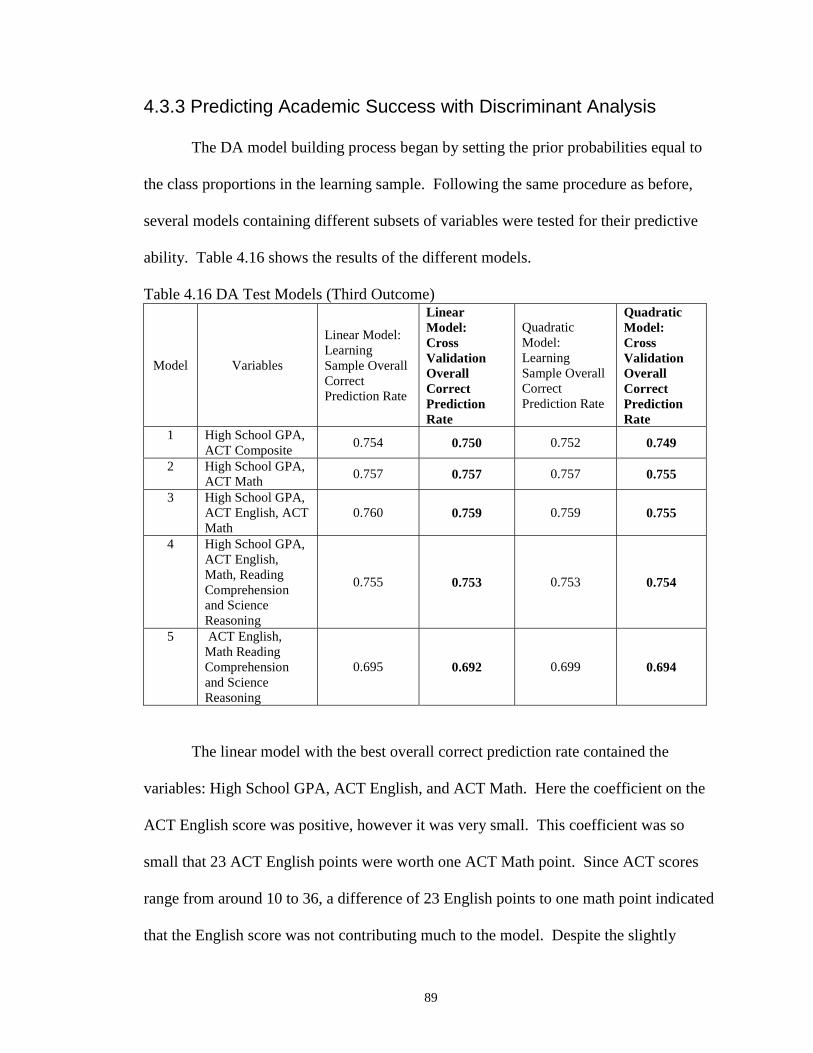
4.16 DA Test Models (Third Outcome) …………………………………………… 89
4.17 DA Confusion Matrix (Third Outcome) ……………………………………... 90
Page 7
vii
6.1 Second Outcome Class and Third Outcome Class Statistics ……………..…. 103
6.2 High School GPA and ACT Math Score ……………………………………. 104
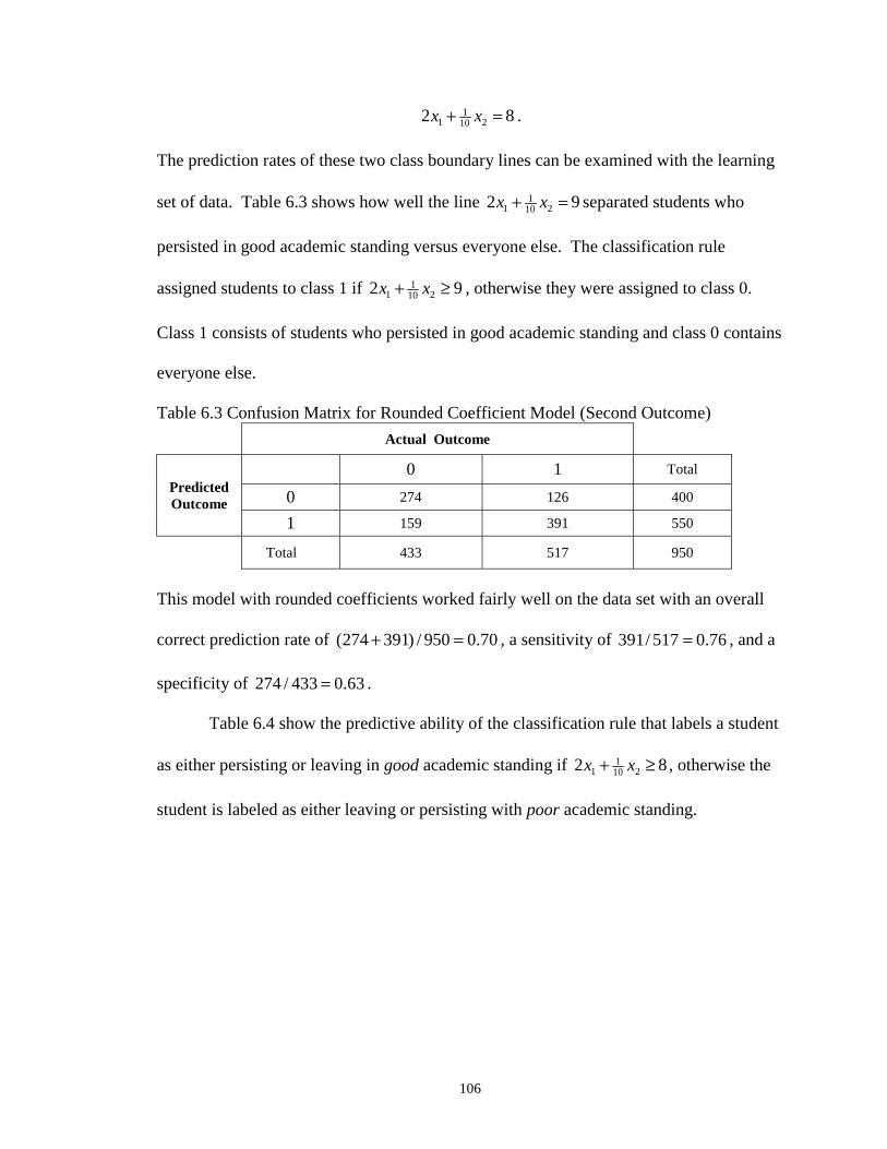
6.3 Confusion Matrix for Rounded Coefficient Model (Second Outcome)...…… 106
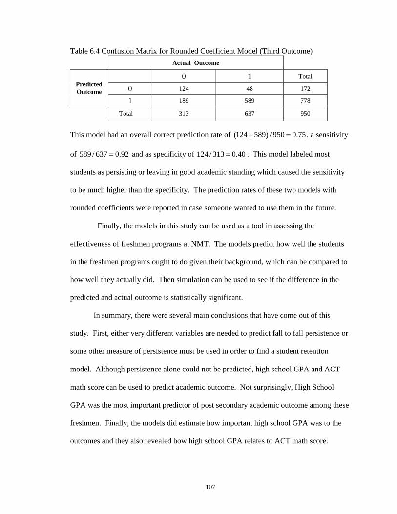
6.4 Confusion Matrix for Rounded Coefficient Model (Third Outcome) ...…….. 107
A.1 Logistic Regression Model for Predicting Fall to Fall Persistence in GoodAcademic Standing ………………………………………………………….. 110
A.2 Logistic Regression Model for Predicting Good Academic Standing ………. 111
Page 8
viii
List of Figures
1.1 CART Example……………………………………………………………… 9
2.1 Percentage of Freshmen Persisting from Fall to Fall by Year ……………… 19
2.2 Percentage of Freshmen Persisting in Good Academic Standing by Year .… 19
2.3 Percentage of Freshmen in Good Academic Standing by Year ……………. 20
2.4 Sex ………………………………………………………………………….. 21
2.5 Ethnicity …………………………………………………………………… 22
2.6 New Mexico High School ………………………………………………….. 22
2.7 First Semester Math Course ………………………………………………… 23
2.8 Percentage of Undecided Majors …………………………………………... 24
2.9 Boxplots of High School GPAs …………………….……………………... 26
2.10 Boxplots of ACT Composite Scores ………………………………………... 27
2.11 Boxplots of ACT English Scores …………………………………………… 27
2.12 Boxplots of ACT Mathematics Scores ……………………………………… 28
2.13 Boxplots of ACT Reading Comprehension Scores ….……………………… 28
2.14 Boxplots of ACT Science Reasoning Scores …………………………….…. 29
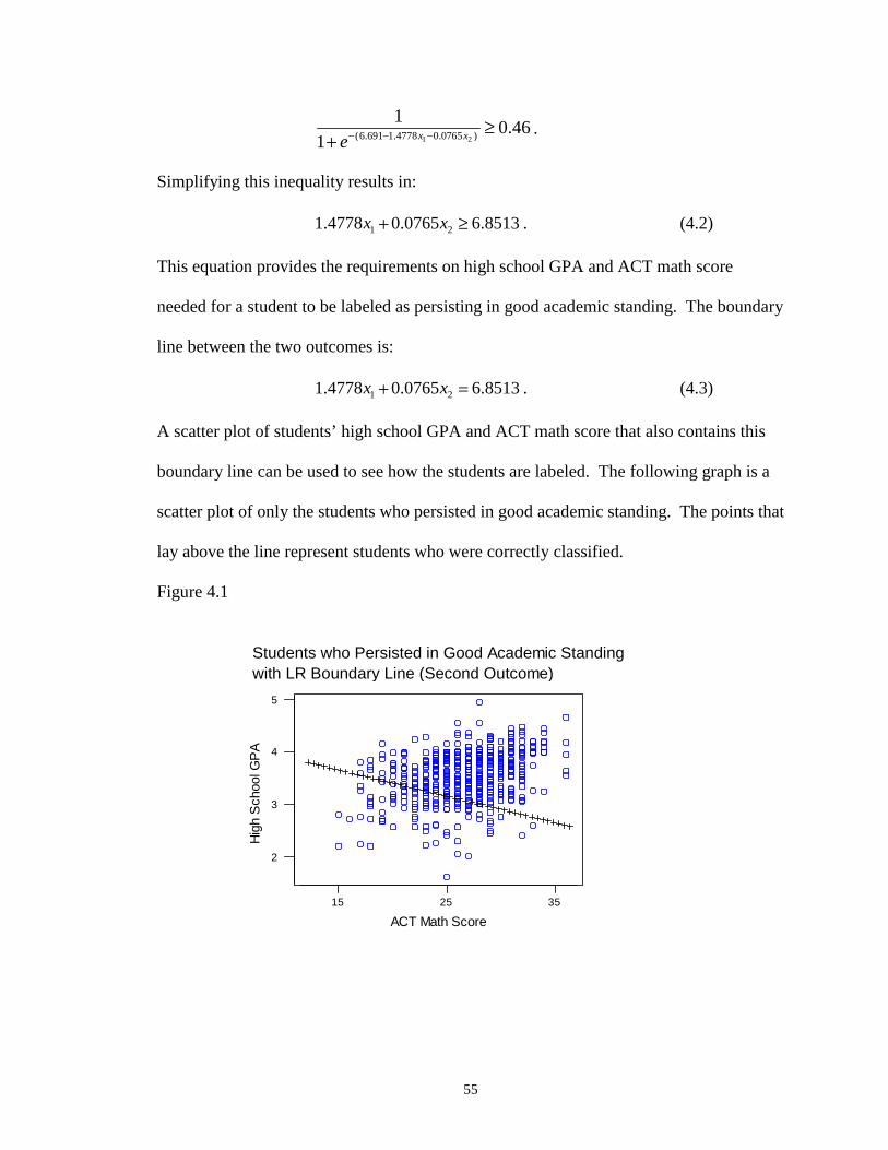
4.1 Students who Persisted in Good Academic Standing and LR Boundary Line (Second Outcome) ……………………………………………………… 55
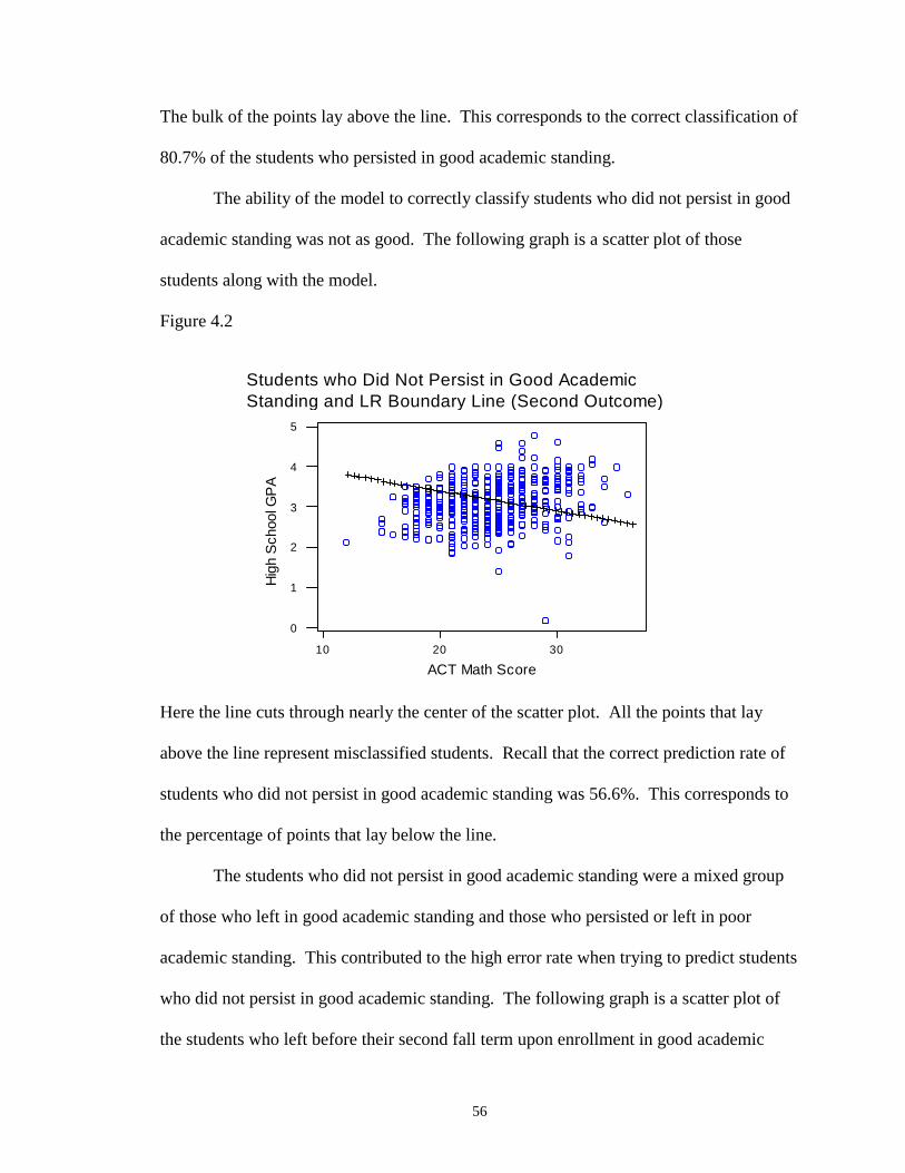
4.2 Students who Did Not Persist in Good Academic Standing and LRBoundary Line (Second Outcome) ……………………………………….…... 56
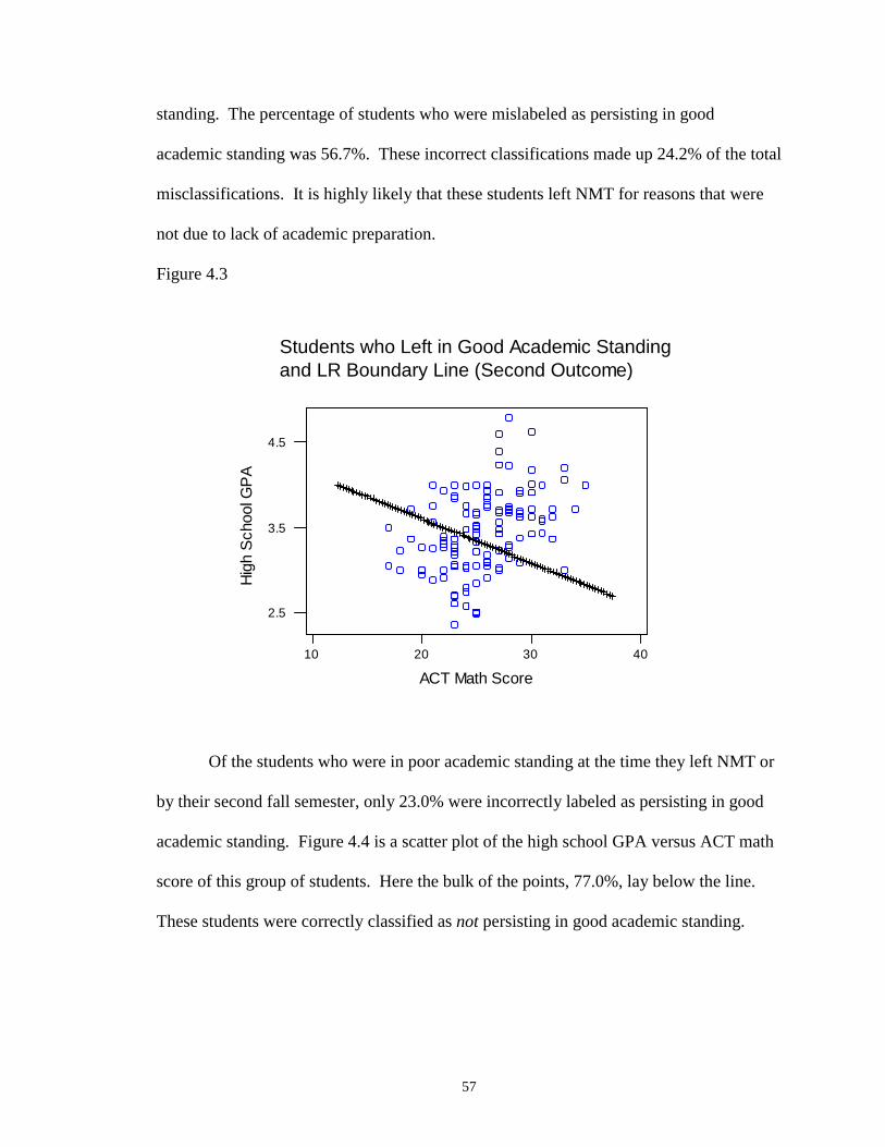
4.3 Students who Left in Good Academic Standing and LR Boundary Line(Second Outcome) ……………………………………………………………. 57
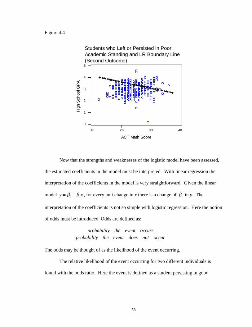
4.4 Students who Left or Persisted in Poor Academic Standing and LRBoundary Line (Second Outcome) …………………………………………… 58
4.5 Preliminary CART Model (Second Outcome) ……………………………….. 63
Page 9
ix
4.6 Final CART Model (Second Outcome) ………………………………………. 65
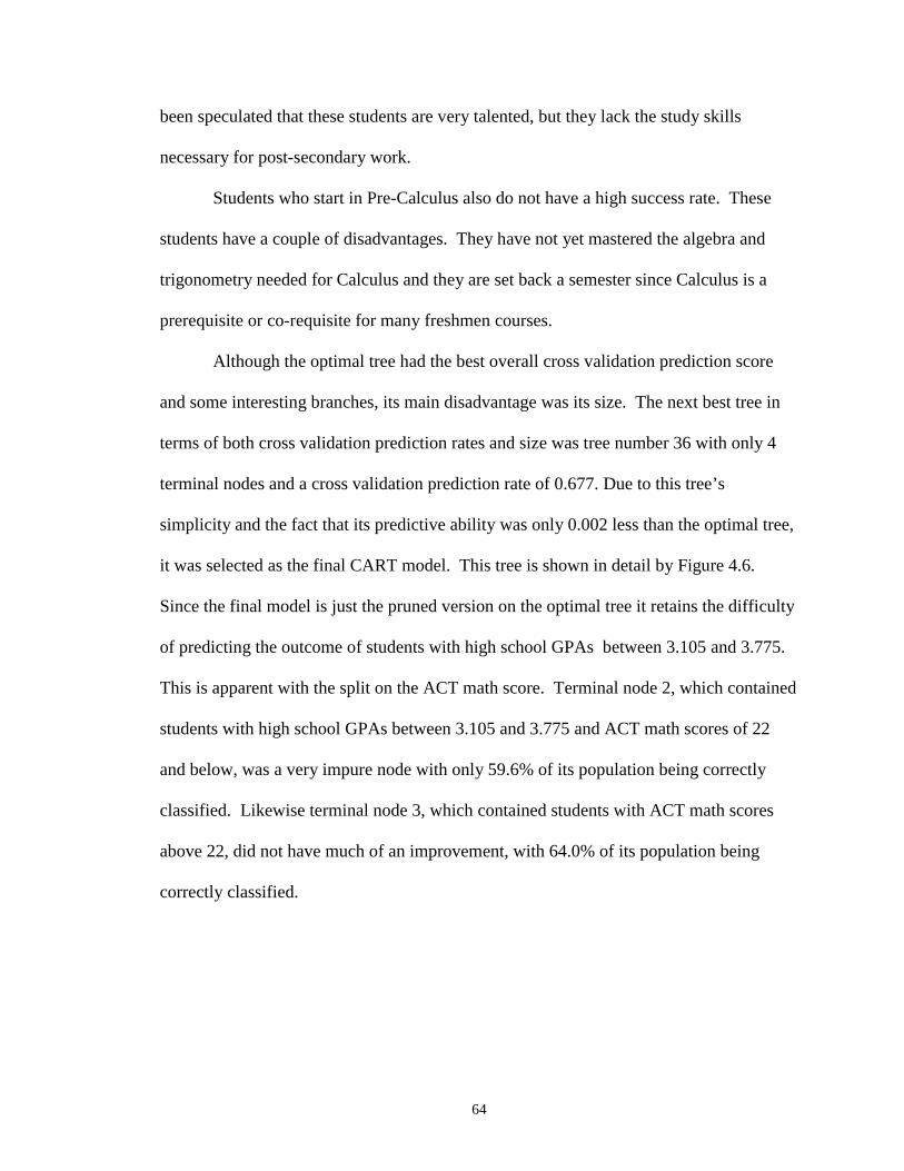
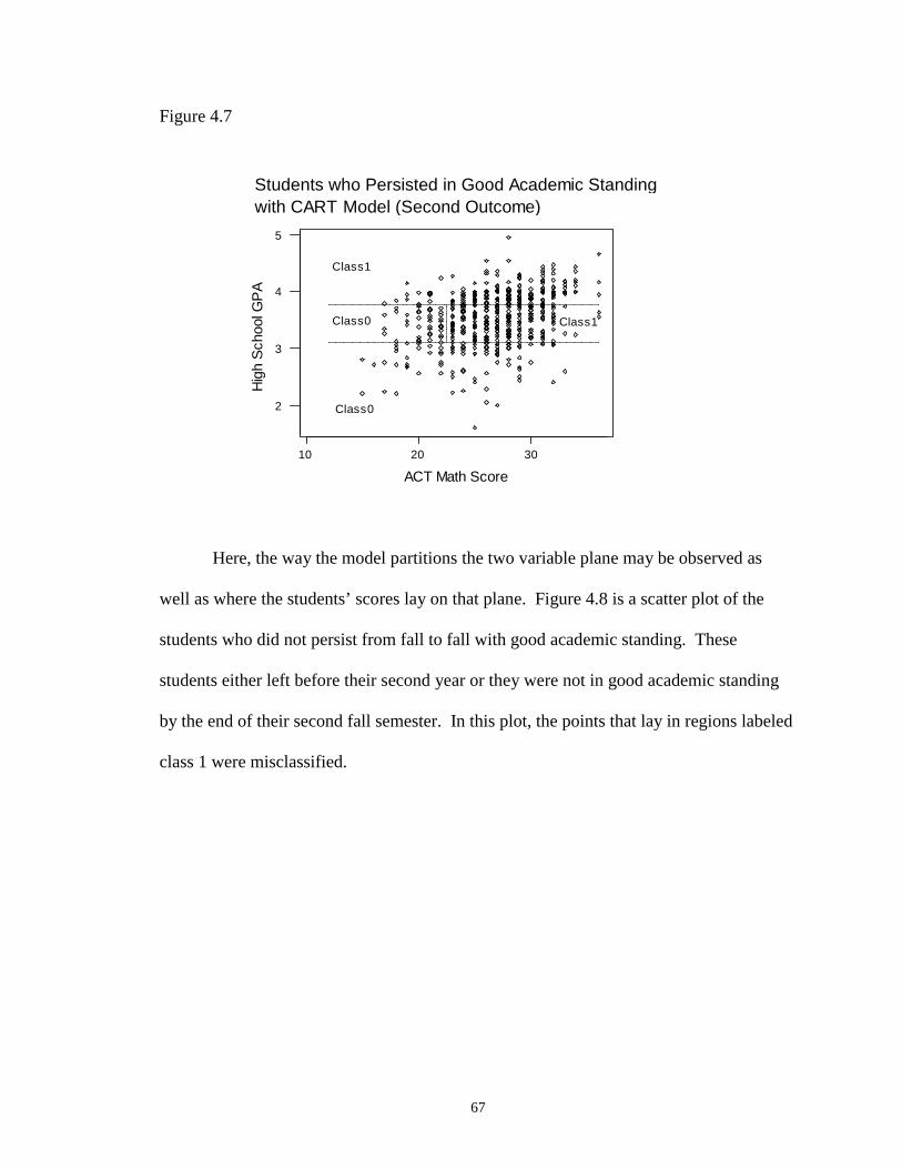
4.7 Students who Persisted in Good Academic Standing and CART Model (Second Outcome) …………………………………………………………….. 67
4.8 Students who Did Not Persist in Good Academic Standing and CARTModel (Second Outcome) ……………………………………………………... 68
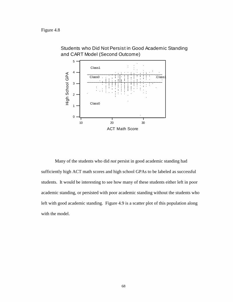
4.9 Students who Left or Persisted in Poor Academic Standing and CARTModel (Second Outcome) …………………………………………………….. 69
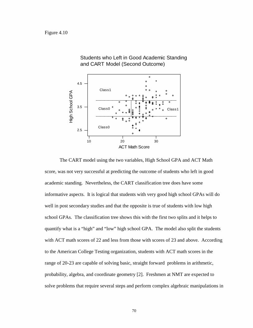
4.10 Students who Left in Good Academic Standing and CART Model(Second Outcome) ……………………………………………………………. 70
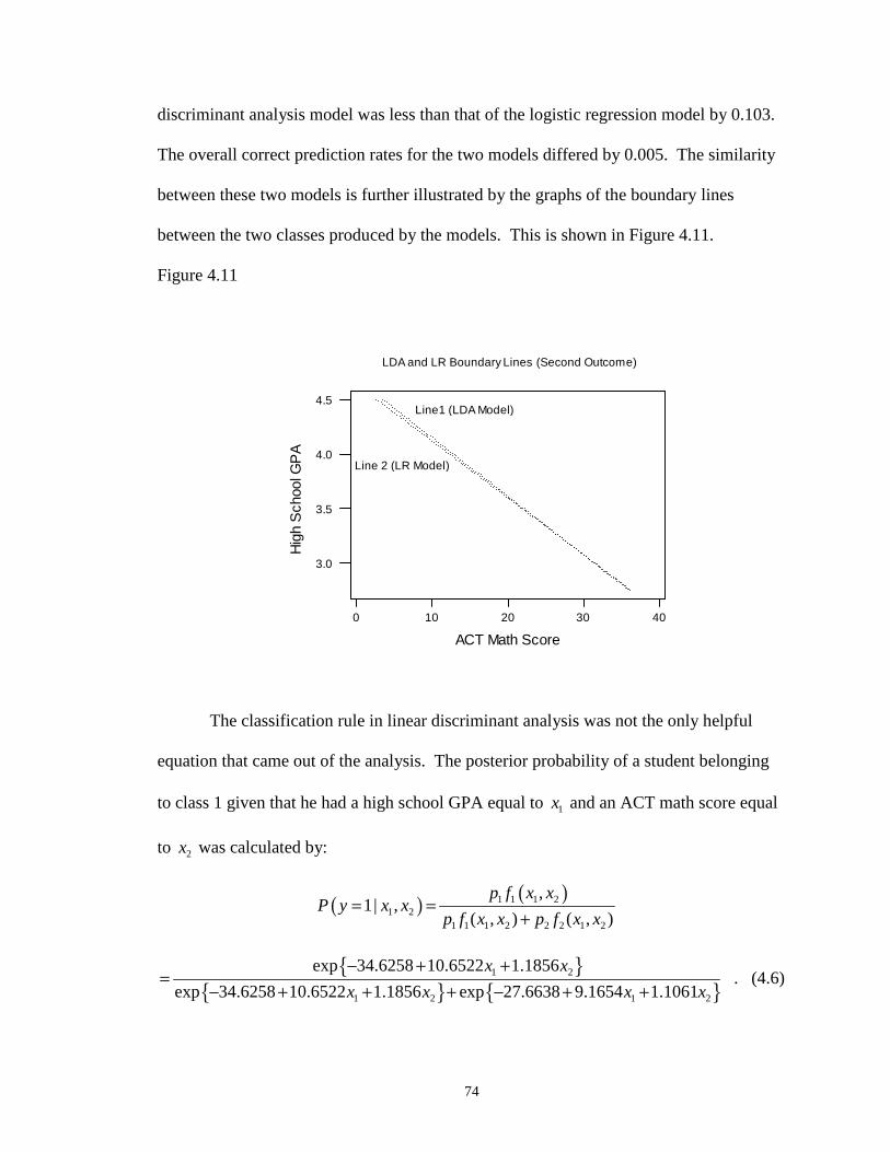
4.11 LDA and LR Boundary Lines (Second Outcome) …………………………….. 74
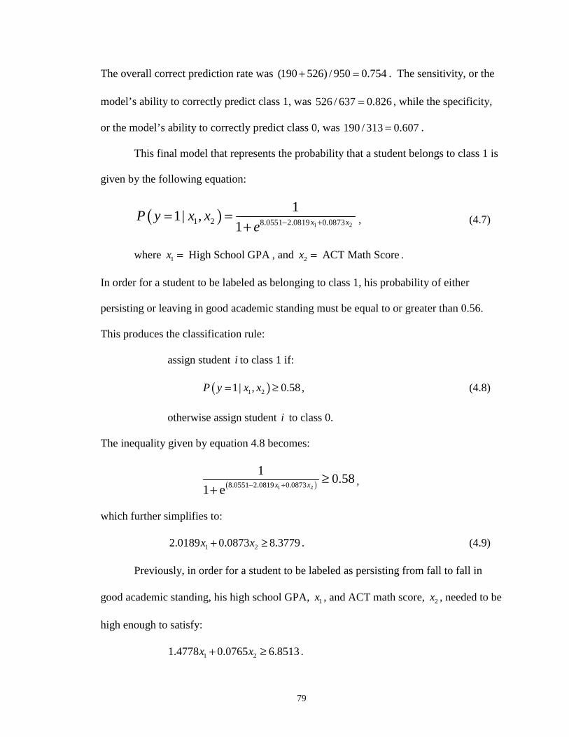
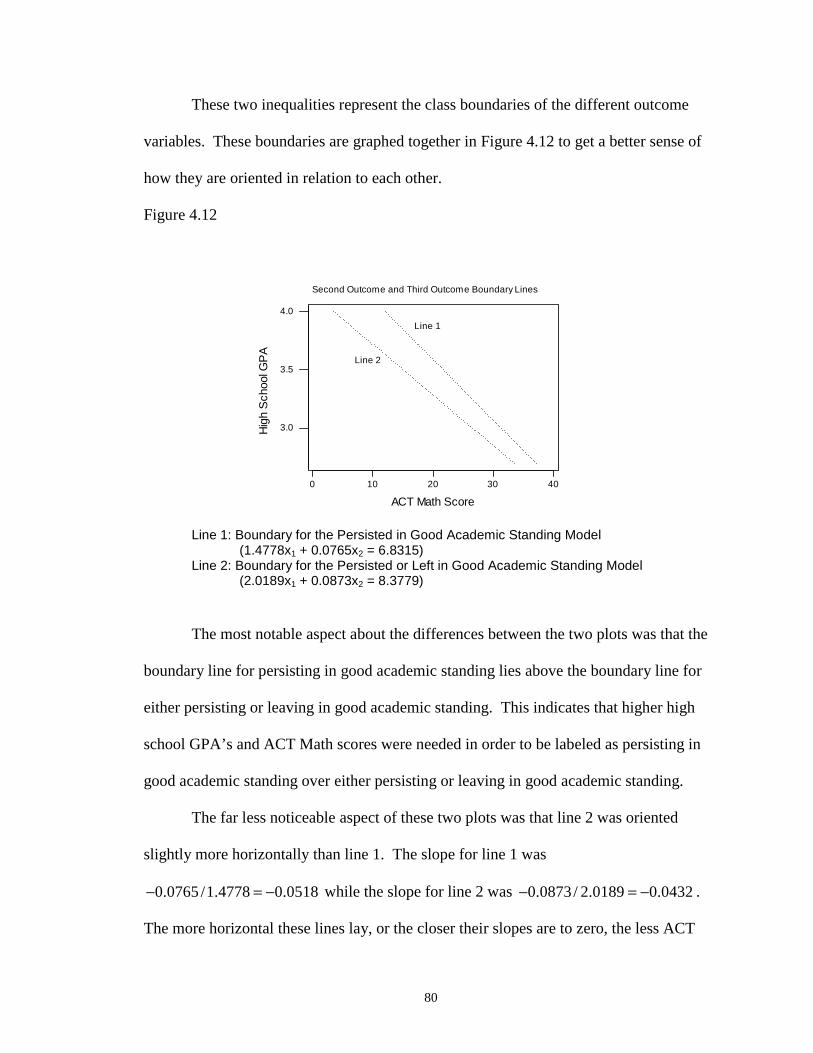
4.12 Second Outcome and Third Outcome Boundary Lines ………………………. 80
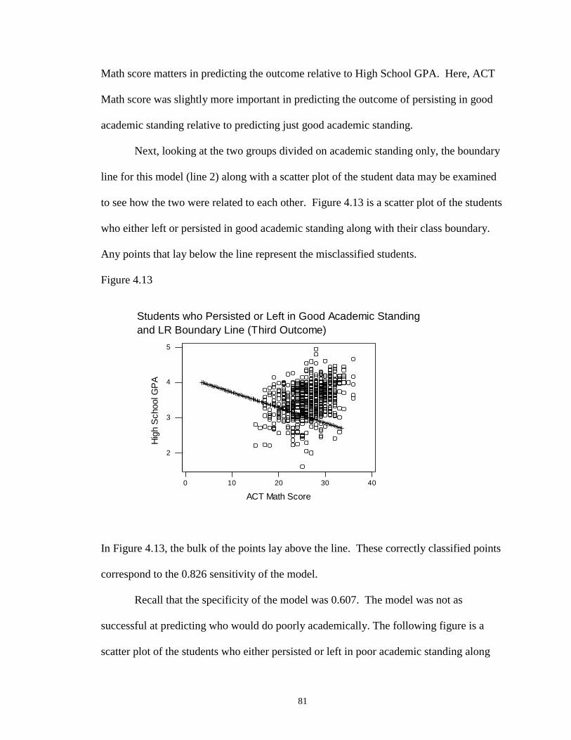
4.13 Students who Persisted or Left in Good Academic Standing and LRBoundary Line (Third Outcome) ……………………………………………... 81
4.14 Students who Persisted or Left in Poor Academic Standing and LRBoundary Line (Third Outcome) ……………………………………………... 82
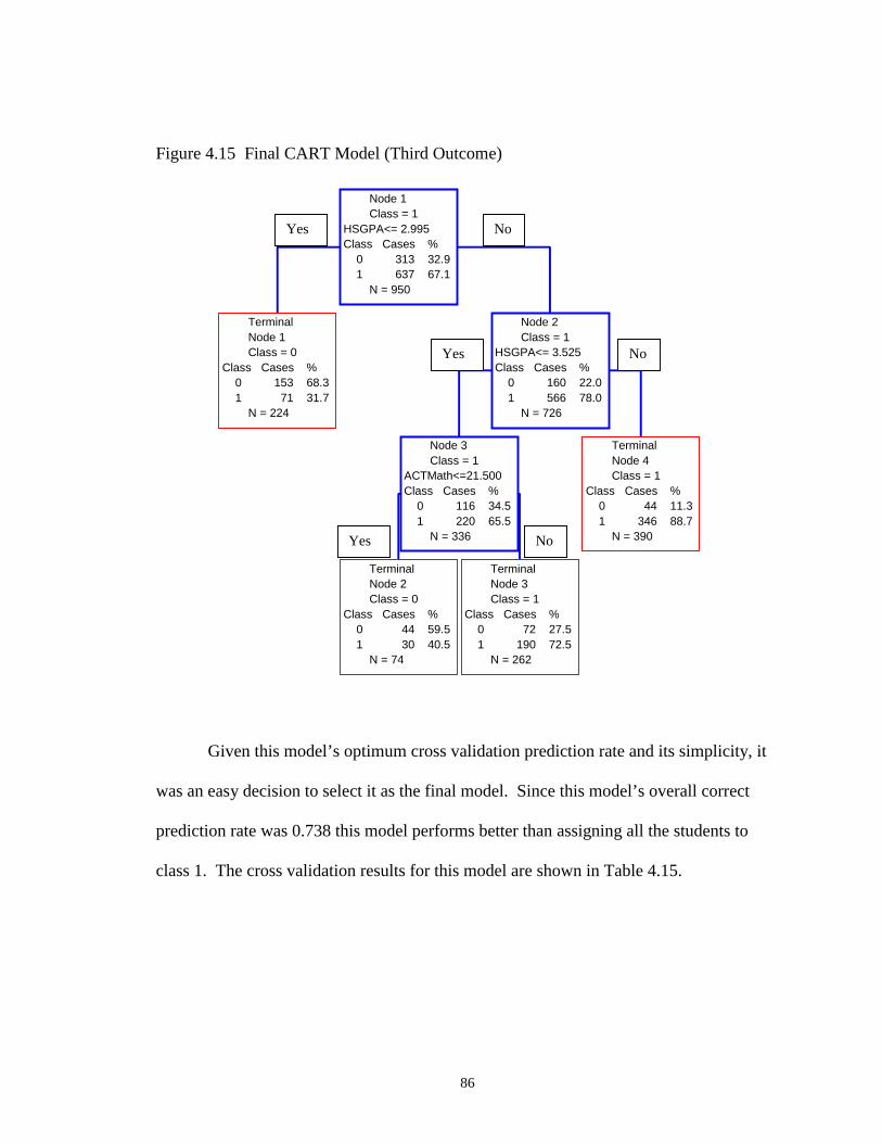
4.15 Final CART Model (Third Outcome) ………………………………………… 86
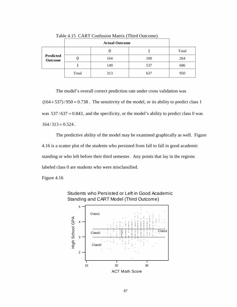
4.16 Students who Persisted or Left in Good Academic Standing andCART Model (Third Outcome) ………………………………………………. 87
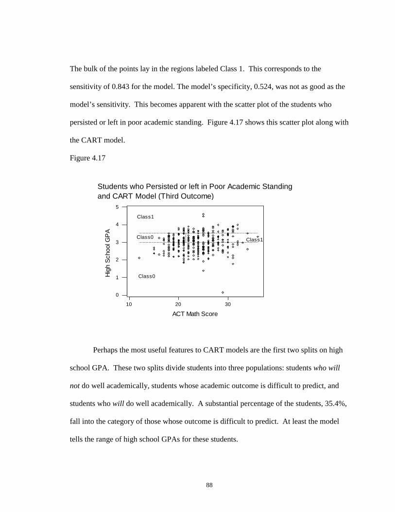
4.17 Students who Persisted or Left in Poor Academic Standing andCART Model (Third Outcome) ………………………………………………. 88
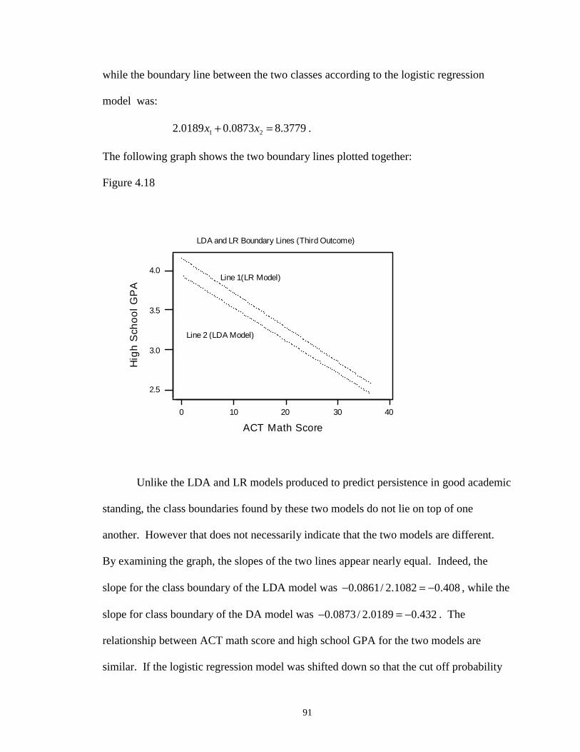
4.18 LDA and LR Boundary Lines (Third Outcome) ……………………………… 91
4.19 LDA and Revised LR Boundary Lines (Third Outcome) …………………….. 92
Page 10
1
1. Introduction
1.1 Background
High rates of student attrition have been a concern at the New Mexico Institute of
Mining and Technology or New Mexico Tech (NMT) for the past several years. Many
inquiries have been made to determine whether new students are adequately prepared for
post secondary work or if the institution is fostering an academically healthy environment
for its students. As part of a continuing effort to improve student retention and academic
performance at NMT, this study investigated three types of mathematical models used to
predict student persistence and good academic performance. These models classify
students as likely or unlikely to persist or do well academically based on variables taken
from their past academic record and their experience during their first semester at NMT.
There were three main objectives in this study. The first was to find classification
models of different outcomes with acceptable prediction rates. These outcomes were
based upon student retention and academic success. In the process of developing the
models, the second objective was to uncover the influential factors that lead to accurate
classification. Hopefully, by gaining a better understanding of these factors, the school
can find new ways to improve student retention and academic performance. Finally, the
third objective was to determine if the freshman program, GOAL, was effective at
retaining students and helping them academically.
The population of this study was first-time freshmen entering NMT in the fall or
summer semesters from 1993 through 1997. These freshmen were full-time or part-time,
degree-seeking students. Freshmen entering in the spring semesters were excluded from
the study for a few reasons. Most first-time freshmen enter NMT in the fall semester.
Page 11
2
NMT also offers these students special programs in their first fall semester or in the
preceding summer semester. Finally, the Council of University Presidents issues the
Performance and Effectiveness Report of New Mexico’s Universities that measures
freshmen progress only with freshmen who entered in summer and fall semesters,
excluding those students who entered in the spring semester [7].
Another standard measurement in the Performance and Effectiveness Report of
New Mexico's Universities for first-time freshmen is fall to fall persistence. Fall to fall
persistence is defined as a student entering in the fall (or preceding summer) and still
being enrolled in the institution the following fall semester [7]. Often in this study, fall to
fall persistence is referred to as just “persistence”. This definition provided a basis for the
three sets of outcome variables in this study.
The three sets of outcome variables consisted of combinations of four different
groups of students. These four groups were defined as follows:
Group 1: Students who persisted fall to fall in good academic standing.
Group 2: Students who persisted fall to fall in poor academic standing.
Group 3: Students who did not persist in good academic standing.
Group 4: Students who did not persist in poor academic standing.
Here, the definition of good and poor academic standing is different than the definition
used by NMT. At NMT, academic standing is based upon a sliding scale, depending on
the number of hours completed. For the purposes of this study, good academic standing
was defined as a student having a cumulative grade point average by the end of his third
semester greater than or equal to 2.0 on a 4.0 scale. If the student left before his third
semester, then he is considered to be in good academic standing if his cumulative grade
Page 12
3
point average was greater than or equal to 2.0 at the last semester of his enrollment. If a
student left before the tenth week of his first semester, then he was not included in the
study, but if a student left after his tenth week, but before grades were issued then he
would have been recorded as not persisting in poor academic standing.
All the outcome variables were binary, separating the students into class 1 or class
0 given the dichotomous nature of persistence. Although the cumulative college grade
point average, instead of academic standing, could have been modeled as a continuous
variable, it was not considered in this study. The first outcome variable was based upon
fall to fall persistence only. Here, class 1 consisted of groups 1 and 2, students who
persisted from fall to fall whether they were in good academic standing or not. Class 0
consisted of groups 3 and 4, students who all left before their second year.
The second outcome variable combined both fall to fall persistence and good
academic standing. Here, class 1 consisted only of group1, students who persisted from
fall to fall in good academic standing. Class 0 consisted of everyone else, students who
persisted or left in poor academic standing and students who left in good academic
standing.
In the process of developing prediction models for the first two outcome
variables, it became apparent that it would be interesting and helpful to investigate a third
outcome variable based upon academic performance only. Thus, for the third outcome
variable, class 1 consisted of groups 1 and 3, students who were in good academic
standing either at the end of their third semester or at the time they left NMT. Class 0
consisted of groups 2 and 4, students who were in poor academic standing either at the
end of their third semester or at the time they left.
Page 13
4
The independent or predictor variables fell into three main categories. These
were the students' personal information, high school background, and first semester
experience. The personal information recorded for each student was:
1. Ethnicity
A. Caucasian vs. Everyone Else
2. Sex
The two-group break up of the variable, Ethnicity, separated students who marked
their predominant ethnic background on their undergraduate application form as
Caucasian versus any other predominant ethnic background which were: Black, Hispanic,
Asian/Pacific, and American Indian. Furthermore, the “Everyone Else” category
included a few students who were labeled as non-resident alien. There were very few
students who were recorded as Black, non-resident alien, or American Indian, therefore
they were clumped together into one category for the Ethnicity variable along with
students recorded as Hispanic.
The high school information was:
1. High School Grade Point Average ( High School GPA)
2. ACT Scores
A. Composite, English, Mathematics, Reading Comprehension, Science
Reasoning
3. Location/ Type of High School Education
A. New Mexico High School versus Non-New Mexico High School
Finally, the variables taken from the students' first semester experience were as
follows:
Page 14
5
1. First Semester Math Course Taken
A. Pre-Calculus versus Calculus
2. Major
A. Undecided versus Decided
There are a couple of comments that need to be made about the first semester
predictor variables. If a student did not take a math course his first semester he was
excluded from the study. It was suspected that if a student in this data set did not take a
math course his first semester then it was likely that he was not a freshmen when he first
enrolled. There were only 27 students in the data set who did not have a math course
their first semester. Also, the school has a special category for students who are
undecided about which branch of engineering to pursue. These students were labeled as
decided in this study since they were more likely to persist from fall to fall in good
academic standing than students who were completely undecided about their major.
Therefore, only students who were completely undecided about their major their first
semester were labeled as undecided.
1.2 Description of Classification Models
Based on a set of measurements of a student, a classification model predicts the
outcome class of that student. These models are created with a learning set of data where
the outcomes of the students are already known. There were two of different ways the
classification models were developed in this study. For the parametric methods, it was
assumed that the students’ measurements belong to some underlying probability
distribution. Based upon this assumed distribution a probability for a student belonging
to a given class could be found and in turn, based upon this probability the outcome class
Page 15
6
of the student could be predicted. For the non-parametric method, the learning set of data
was searched through to find the features that most differentiated the two classes. For
both the parametric and non-parametric methods, once the class probability distributions
or the differential features had been assessed, a classification rule was derived that would
assign a student to a class based upon the student’s measurements.
Often different populations share similar characteristics. This makes it difficult to
separate them and a student may be assigned to the wrong class. A good discrimination
and classification procedure should result in few misclassifications. Furthermore, when
trying to correctly classify one population, the model should have a higher success rate
than the given percentage of that population in the overall data set. For example, if 85%
of the objects in the group we want to separate and classify belong to population A and
15% belong to population B, then we could simply classify all the objects as belonging to
population A and we would be correct 85% of the time. In order to be certain that the
predictor variables actually tell something about the outcome, a model must be found
that has a higher prediction rate than 85%.
The models’ prediction rates on the learning data set are likely to be
overestimates of how well the model will predict future observations since the learning
data set was used to build the model. One common way of assessing a model’s ability to
predict future observations is to break the data set into two subsets. One subset is used to
build the model and the other subset is used to find the model’s misclassification rates.
Unfortunately, this requires a large data set.
Another common way to test a model’s true predictive ability is with cross
validation. There were two types of cross validation used in this study; 10-fold cross
Page 16
7
validation and “leave one out” cross validation. In 10-fold cross validation, 10% of the
data is set aside and a model is built with the remaining 90%. The misclassification rates
on the separate 10% of data are found. The process is repeated for a different 10% of the
data set and the remaining 90% are used to create the model until the entire data set has
been used as a test sample. Next, using all the data, the final model is created. The true
error rate of this model is estimated to be the average of all the error rates from the ten
test models. “Leave one out” is a more intensive cross validation technique. Here, one
data point is left out of the learning sample, a test model is built with the remaining
observations and then the test model is used on the one point left out. This process
continues for all the data points. Again, the final model is created using all the data, but
its estimated error rates are determined by how well the test models predicted the
outcome of “points left out”.
Throughout the model building process, a model with fewer variables was
preferred if its prediction rate was similar to a model with more variables. Although it
may seem paradoxical, models with more variables may lead to less predictive accuracy.
This problem occurs when the model “overfits” the learning sample. An overfitted model
can predict the outcomes of the data set that was used to build it very well, but it may
work poorly at predicting the outcomes of a new data set. This occurs because most data
sets have unusual observations, and the overfitted model would be good at predicting the
unusual observations at the expense of not representing the general trend of the data.
Although including too many variables could lead to an overfitted model, it would be
equally detrimental to not include an important variable. This leads to the difficulty in
Page 17
8
selecting predictor variables for most models. For each of the models in this study, the
variable selection process was described in detail.
1.3 Three Different Classification Methods
Logistic Regression (LR)
Logistic regression is a parametric method that is based upon the assumption that
the probability of the event occurring follows a logistic distribution. In this case, the
event is that a student belongs to a certain group called class 1. The logistic distribution
allows for all types of variables. This distribution is defined as follows:
( ) 11|
1TP outcome
e β−= =
+ XX
where 0 1 1 2 2 ...Tk kx x xβ β β β β= + + + +X and X is a set of measurements,
[ ]1 2, ,...,T
kx x x=X .
The logistic distribution has many good attributes. It is bounded by zero and one,
which is necessary to represent probabilities. Also, the distribution is in the shape of an
“S”. This indicates that small differences at the extreme values of the predictor variable
do not influence the outcome nearly as much as differences around the center [8]. For
example, it might not make much of a difference in a student’s probability of dropping
out if his high school grade point average was a 2.0 or a 2.5, nor if his high school grade
point average was a 3.5 or a 4.0. However, there may be a large difference in the
probability of a student persisting depending if his high school grade point average was a
2.5 or a 3.0.
Page 18
9
This leads to the logistic distribution’s ability to separate and predict binary
outcomes. The upper portion of the “S” represents high probabilities of the event
occurring and the lower portion of the “S” represents low probabilities of the same event
occurring. These two portions determine the two outcomes. The difficulty lies in
deciding where to cut the “S” and separate the two outcomes [8].
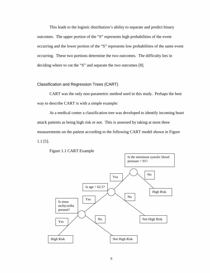
Classification and Regression Trees (CART)
CART was the only non-parametric method used in this study. Perhaps the best
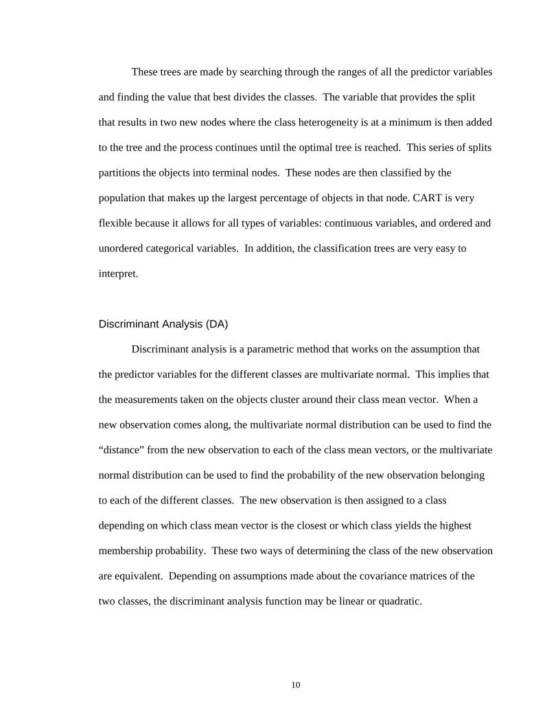
way to describe CART is with a simple example:
At a medical center a classification tree was developed to identify incoming heart
attack patients as being high risk or not. This is assessed by taking at most three
measurements on the patient according to the following CART model shown in Figure
1.1 [5].
Figure 1.1 CART Example
T
Is the minimum systolic bloodpressure > 91?
NoYes
High Risk
Is age > 62.5?
NoYes
Not High Risk
Is sinustachycardiapresent?
NoYes
High Risk Not High Risk
Page 19
10
These trees are made by searching through the ranges of all the predictor variables
and finding the value that best divides the classes. The variable that provides the split
that results in two new nodes where the class heterogeneity is at a minimum is then added
to the tree and the process continues until the optimal tree is reached. This series of splits
partitions the objects into terminal nodes. These nodes are then classified by the
population that makes up the largest percentage of objects in that node. CART is very
flexible because it allows for all types of variables: continuous variables, and ordered and
unordered categorical variables. In addition, the classification trees are very easy to
interpret.
Discriminant Analysis (DA)
Discriminant analysis is a parametric method that works on the assumption that
the predictor variables for the different classes are multivariate normal. This implies that
the measurements taken on the objects cluster around their class mean vector. When a
new observation comes along, the multivariate normal distribution can be used to find the
“distance” from the new observation to each of the class mean vectors, or the multivariate
normal distribution can be used to find the probability of the new observation belonging
to each of the different classes. The new observation is then assigned to a class
depending on which class mean vector is the closest or which class yields the highest
membership probability. These two ways of determining the class of the new observation
are equivalent. Depending on assumptions made about the covariance matrices of the
two classes, the discriminant analysis function may be linear or quadratic.
Page 20
11
Since DA works under the assumption that the predictor variables are normally
distributed, only continuous predictor variables were allowed to be candidates for entry in
the final model. Binary variables simply cannot be normally distributed and therefore
should not be used with this method. This is the main disadvantage of discriminant
analysis since binary or categorical variables may be very informative about the outcome.
However, the histograms of all the continuous variables for this study were
approximately normal.
1.4 Previous Studies
Lim, Loh, and Shih compared thirty-three classification algorithms with various
data sets in 1998 [11]. CART, logistic regression, and both linear and quadratic
discriminant analyses were included in this study. These researchers empirically
investigated the accuracy and the relative time needed to build each model (running time)
of these and other classification algorithms. They used a total of thirty-two data sets.
Fourteen of the data sets were taken from real-life studies and two were simulated data.
These data sets ranged in size from 3,772 to 151 observations. The number of data sets
was then doubled by adding noise to each of the original data sets.
Amongst all thirty-three classification algorithms in this study, logistic regression
and linear discriminant analysis performed exceptionally well at correctly predicting class
outcome. The two versions of CART performed marginally well, and finally quadratic
discriminant analysis performed very poorly in classification accuracy. None of these
algorithms had median running times in hours. Logistic regression had the longest
Page 21
12
median running time of four minutes. The other algorithms, CART and discriminant
analysis, had median running times of less than a minute.
It is interesting to note how well linear discriminant analysis performed despite
the requirement for predictor variables to be normally distributed. In another study done
by Meshbane and Morris, the predictive accuracy of logistic regression and linear
discriminant analysis were compared [12]. In their presentation, Meshbane and Morris
list the many conflicting reports about which classification method works better for non-
normal predictors and for small sample sizes. It was concluded that there is no specific
type of data set that favors logistic regression or linear discriminant analysis. Instead the
classification accuracy of both logistic regression and linear discriminant analysis should
be carefully compared to determine which may provide a better model.
This leads to the comparison of logistic regression and linear discriminant
analysis in Eric L. Dey’s and Alexander W. Astin’s study of college student retention [8].
Astin previously equated linear discriminant analysis to linear regression [8]. In their
study, Dey and Astin used logistic and linear regression to predict whether first-time,
full-time community college freshmen who intend to earn a two-year degree would
graduate on time. They also tried predicting less stringent expectations of the students
such as completing two years of college, or being enrolled for a third consecutive fall
semester upon admission. They used predictor variables that “were shown to predict
retention among students at four-year colleges and universities” [8]. These predictor
variables included students’ concern about ability to finance their education, their
motives for attending college, how many hours they spent per week at various activities
their first year, and their high school grade point average.
Page 22
13
In their results, Dey and Astin did not find any important differences between
logistic and linear regression. Both methods indicated that a student’s high school grade
point average was the strongest positive predictor of earning a degree in two years.
These methods also indicated that a student’s concern over finances and motivations to
attend college in order to earn money were significant negative predictors of retention.
Each of the techniques had similar classification accuracy as well [8].
Although Dey and Astin claimed that the methods used in linear regression are
analogous to those used in linear discriminant analysis [8], no discriminant model was
created. However, discriminant models have been used to predict student success.
Hamdi F. Ali, Abdulrazzak Charbaji, and Nada Kassin Hajj used linear
discriminant functions in their study to see what admission criteria could help predict
student success at Beirut University College (BUC) in Lebanon [4]. BUC had the
problem of having far more applicants than space for these aspiring students. Not only
had the number of applicants to BUC increased, but also the number of students who
were on academic probation had increased. Ali, Charbaji, and Hajj developed three
different linear discriminant models for each of the divisions at the school: business,
natural sciences, and humanities.
In their learning sample, the researchers only chose students who were on the
dean’s list with grade point averages greater than 3.2 or on academic probation with
grade point averages less than 2.0 in their second year at the college. These two
populations determined the outcome variables. The predictor variables were taken from
admission information which included high school grade point average, scores from a
college entrance exam, type of high school (public or private), relevant language skills,
Page 23
14
personal characteristics, and finally the type of government certificate (did the student
pass an official public exam or were they given a statement of candidacy due to the civil
war). In the analysis, the researchers decided to use the interactive effects of these
variables.
Ali, Charbaji, and Hajj were satisfied with the predictive ability of all three
discriminant models for each academic division. Each model had slightly different
predictive variables. The variables chosen for the science division were:
Score on college entrance exam * High school grade point average
Score of college entrance exam * Type of high school
Score of college entrance exam * Sex
High school grade point average * Type of certificate
Overall students who passed the public exams and women were less likely to be
on probation. In the natural sciences division, students from private schools and those
with high college entrance exam scores and good high school grade point averages were
also less likely to be on probation.
Although discriminant analysis and logistic regression are well known in college
student retention studies, CART holds promises for being a good classification model.
CART does not depend on any underlying structure of its variables and it also provides
an easy-to-interpret graphical model. Using a wide array of classification models allows
for the problem of predicting student attrition to be approached from many different
perspectives.
Page 24
15
2. Data Collection and Preliminary Analysis
In this chapter, the procedures used to collect the data set in this study are
described. This description is intended to provide documentation for the data set so that
the study may be repeated and so that student information can be retrieved in a similar
manner if future predictions of student outcome are to be made. In addition to describing
the methods used for collecting the data, this chapter also contains the preliminary
analysis where the data set is examined for trends over the years. If there were any strong
trends in the data then it would not be appropriate to use a single prediction model to try
to determine class outcome for all the years together. However, if the distributions of the
variables remained steady over the period from 1993 to 1997, then it would be safe to
assume that the distributions of the current student population are the same as those of
past students.
All the data for this study was collected from the student database provided by the
Registrar’s office at NMT. Although this database contained several tables, only four
were needed to collect the student data. Here is a summary list of the tables used and the
data collected from them.
Table 2.1 Student Database Tables
Table in the Student Database Student Information Collected
1. APPLICATION 1. High School Information
2. STUDENT 2. Personal Information
3. STUDENT COURSE 3. First Semester Math Course
4. STUDENT HISTORY 4. Information to Construct the Outcome Classes
Page 25
16
The first step was to query the population of this study: first-time, degree seeking
freshmen. Unfortunately, there was no one specific label for this group of students in the
database. Instead, if a student’s original status was labeled as “new student,” and the
student was labeled as both a freshmen and enrolled for the first time in a degree seeking
program at NMT for a given semester, that student was included in the study. Requiring
students to be both a new student and a freshman might seem redundant, however there
were a few students who were labeled as new students although they entered NMT for
the first time as sophomores, juniors, and seniors. After investigating a few of these
students it was apparent that they were all probably transfer students and they needed to
be excluded from the study.
Since the important information identifying new freshmen was contained in three
different tables, it was a complicated process to select students who had the three
requirements of:
1. Enrolling for the first time in a given semester (information contained in the
APPLICATION table)
2. Having original status as “new student” (information found in the STUDENT table)
and
3. Having the status as “freshmen” in the first semester entering NMT (information
found in the STUDENT HISTORY table).
For one semester, all the students who first enrolled in NMT that semester were
selected by querying students labeled as “enrolled” under the STATUS field in the
APPLICATION table for the given term. From this group, students who were labeled as
“new students” under the ORIGINAL STATUS field in the STUDENT table were
Page 26
17
collected. Finally, this group was further restricted to those students who were labeled as
“freshmen” under STUDENT LEVEL in the STUDENT HISTORY table. Once this
process was completed, a cohort of first-time freshmen for that semester was collected.
Next the groups’ data was collected. The simplest data to collect was the personal
and high school information since it did not depend on any particular semester. A
student’s first term math course was found in the STUDENT COURSE table, where
students’ past courses taken were labeled by the semester the course was taken and by the
course name. Finally, the STUDENT HISTORY table contained past semester
information on students’ declared major, their term grade point average, and the units
they attempted, completed and were graded. The past term grade point averages and
units graded were used to construct the outcome classes. The following table shows the
field name and the table from which the data was collected and the names of the variables
given to this data.
Table 2.2 Variable InformationVariable Field Name Table
1. Ethnicity ETHNIC STUDENT
2. Age BIRTH DATE STUDENT3. Sex SEX STUDENT4. High School GPA GPA APPLICATION
5. ACT Scoresa. Compositeb. Englishc. Mathd. Science Reasoninge. Reading Comprehension
a. ACT COMPb. ACT ENGc. ACT MATHd. ACT NATSe. ACT SOCS
APPLICATION
6. Location/ Type of High SchoolEducation
HS CODE APPLICATION
7. First Term Math Course SECTION KEY STUDENT COURSE
8. Major Declared in First Term MAJOR1 STUDENT HISTORY
9. Outcome Classes (found from termgrade point averages and unitsgraded for the next three semestersupon initial enrollment)
GPA, UNITS GRADED STUDENT HISTORY
Page 27
18
In most cases if a student was missing information there was no way for it to be
replaced. However, if a student did not have ACT scores but he had an SAT equivalent
score, then the SAT combined score replaced the ACT composite score.
Unfortunately, the methods used for logistic regression and discriminant analysis
do not allow for missing data. Therefore, students with missing data were not used to
build these models. In order to be consistent, these students were also excluded in
building the CART models, although CART does allow for missing data.
Once all the data was cleaned and organized, the data was examined to see if the
distributions remained stable over time. Fortunately, all the various distributions were
fairly homogeneous for the different years. Since there were no noticeable trends, the
data from all the years were lumped together to form the learning sample for each
classification model.
The data was examined using graphical methods. Bar charts were used to
investigate the discrete or categorical variables to see if the percentages of the various
categories changed over time. The graphs used to examine the variables over time are
shown in this chapter. Beginning with the three outcome variables, the first outcome
variable was fall to fall persistence versus non-persistence. Figure 2.1 shows the yearly
percentage of freshmen that persist from fall to fall.
The second outcome variable was persistence with good academic standing versus
everyone else. The percentages of students who persisted fall to fall with a cumulative
grade point average of 2.0 or greater is shown in Figure 2.2.
Page 28
19
Figure 2.1
Figure 2.2
Percentage of Freshmen Persisting from Fall to Fall by Year
67.6 68.375.8
70.6 73.3
0.0
10.0
20.0
30.0
40.0
50.0
60.0
70.0
80.0
1993 1994 1995 1996 1997
Year
Perc
enta
ge
Percentage of Freshmen Persisting in Good Academic Standing by Year
59.2
53.652.751.1
55.6
0.0
10.0
20.0
30.0
40.0
50.0
60.0
70.0
1993 1994 1995 1996 1997
Year
Perc
enta
ge
Page 29
20
Despite the modest increases at the end of the five-year period there was no strong
trend among these variables, nor was there one year that was plainly different from the
rest.
The last outcome variable divided students into two groups dependent on
academic standing only. Here class 1 was defined as students who were in good
academic standing at either the end of their third semester or at the time they left NMT.
The bar chart for this variable is shown below.
Figure 2.3
In Figure 2.3, again, there is no trend over the years in the third outcome variable.
These three graphs indicate that the number of students in the different outcome
classes remained steady over the five-year period. Although there was a slight
improvement in student retention between the two groups of years 1993-1995 and 1996-
1997 it is not significant enough to divide the learning data set into two parts.
Percentage of Freshmen Either Leaving or Persisting in Good Academic Standing by Year
67.0 69.4 68.3 68.1
63.0
0.0
10.0
20.0
30.0
40.0
50.0
60.0
70.0
80.0
1993 1994 1995 1996 1997
Year
Perc
enta
ge
Page 30
21
The next set of categorical variables to be examined for trends over the years was
sex, ethnicity, and location of high school. The bar graphs for these plots are given by
Figures 2.4 to 2.6. Here the percentages of male and female students were approximately
70% to 30%. The percentage of Caucasian students was approximately 72%. Finally,
approximately 65% of the students came from high schools located in New Mexico.
Figure 2.4
Sex
68.1 68.670.470.6 70.6
31.9 29.4 29.6 29.4 31.4
0.0
10.0
20.0
30.0
40.0
50.0
60.0
70.0
80.0
1993 1994 1995 1996 1997
Year
Perc
enta
ge o
f Fr
eshm
en
Male Female
Page 31
22
Figure 2.5
Figure 2.6
Ethnicity
74.7
68.3
73.075.3 72.3
25.3 31.7 24.7 27.0 27.7
0.010.020.030.040.050.060.070.080.0
1993 1994 1995 1996 1997
Year
Perc
enta
ge o
f Fr
eshm
en
Caucasian Everyone Else
New Mexico High School
67.864.361.1
69.9
61.3
0.0
10.0
20.0
30.0
40.0
50.0
60.0
70.0
80.0
1993 1994 1995 1996 1997
Year
Perc
enta
ge o
f Fr
eshm
en
Page 32
23
The previous set of bar graphs represented personal and high school information
about the students. The next set of bar graphs involves information found in the students’
first semester. First semester categorical variables consisted of first semester math class
and whether or not the student decided on a major. First semester math classes were
broken up into two categories: Pre-Calculus, and Calculus and above. The variable,
Major, was also broken up into two categories: those who declared a major even if it was
undecided within the engineering departments and those students who were completely
undecided. Please note that this was the major declared the first semester upon enrolling
at NMT and that students often choose to change their majors. Figure 2.7 shows the
percentages of students who began in Pre-Calculus, and those who took Calculus or
above. Figure 2.8 shows the percentages of students who were undecided about their
major their first semester.
Figure 2.7
First Semester Math Course
50.551.7
62.165.4
60.7
37.9
48.3 49.5
34.6 39.3
0.0
10.0
20.0
30.0
40.0
50.0
60.0
70.0
1993 1994 1995 1996 1997
Year
Perc
enta
ge o
f Fr
eshm
en
Calculus and Above Pre-Calculus
Page 33
24
Figure 2.8
The bar chart for the first semester math course is very interesting. In 1994 and
1995 the percentages of students who began in Pre-Calculus and those who began in
calculus or above are about equal. Otherwise there were more students beginning in
calculus and above than there were students beginning in Pre-Calculus. Despite this
anomaly there did not appear to be any distinct trend over time. The number of new
freshmen enrolling at NMT who began in Pre-Calculus was not increasing or decreasing.
The following chart shows that the number of freshmen who were undecided
about their major their first semester fluctuated between 9.3 and 16.1 for the five year
period with no trend up or down over the years.
The distributions of the continuous variables were examined for trends using
boxplots. The continuous variables in this data set were high school grade point average,
and all the various ACT scores. An example boxplot is shown below.
Percentage of Undecided Majors
9.3
15.213.9
16.112.8
0.02.04.06.08.0
10.012.014.016.018.020.0
1993 1994 1995 1996 1997
Year
Perc
enta
ge
Page 34
25
*
To create a boxplot, first the data points are ordered. The middle point in the
ordered data set is called the median. The quartiles, Q2 and Q3 mark the points where
25% of the data lay above and 25% of the data lay below, respectively. These second
and third quartiles mark the limits of the box. The lines that extend from the box are
called whiskers. These whiskers extend 3 21.5( )Q Q− units above and below the box.
Any point that lies beyond the whiskers is considered an outlier, an extreme point, in the
data set.
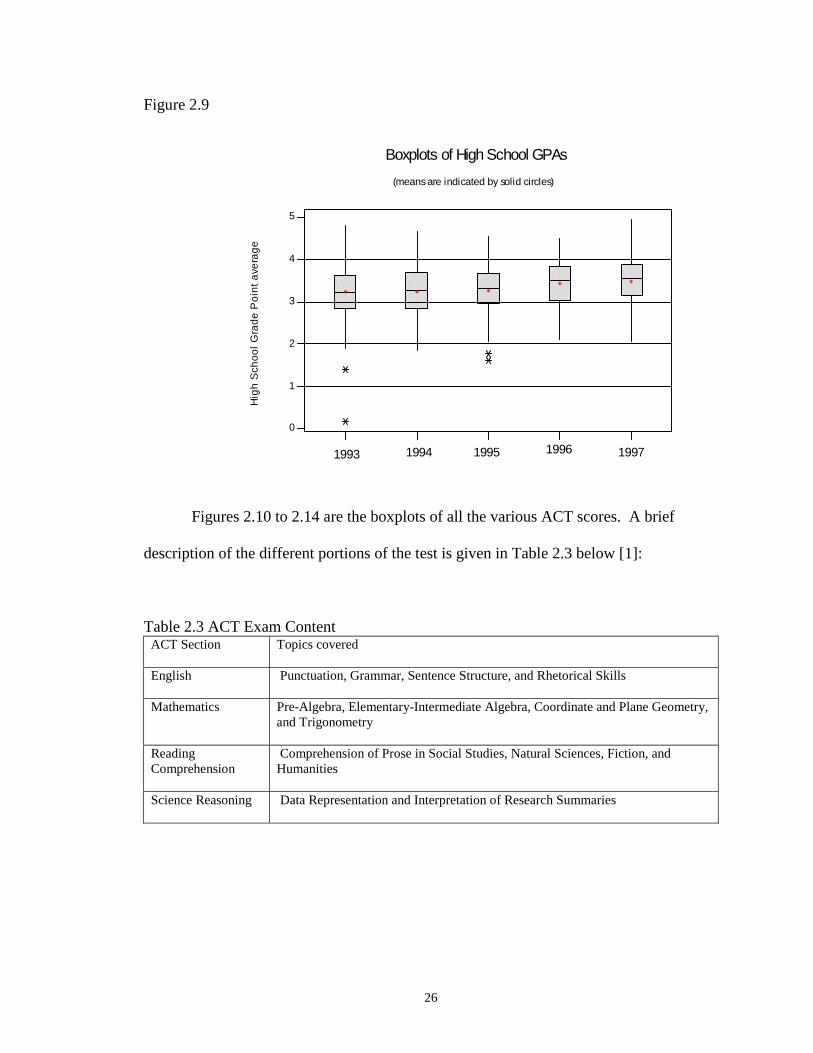
Figure 2.9 contains the boxplots of students’ high school grade point averages for
each year. The circles on these plots indicate the means of the distributions. The high
school grade point averages mostly ranged from 3.0 to 4.0 over the years. There were
four people in 1993 and 1995 who were admitted with high school grade point averages
lower than a 2.0.
Q2 + 1.5(Q3-Q2)
Q2
Median
Q3 – 1.5(Q3 – Q2)
Outlier
Q3
Page 35
26
Figure 2.9
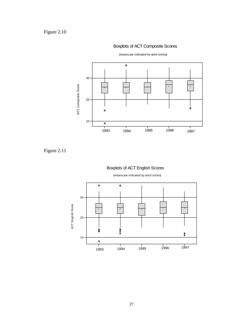
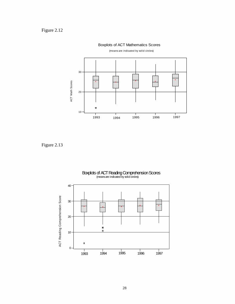
Figures 2.10 to 2.14 are the boxplots of all the various ACT scores. A brief
description of the different portions of the test is given in Table 2.3 below [1]:
Table 2.3 ACT Exam ContentACT Section Topics covered
English Punctuation, Grammar, Sentence Structure, and Rhetorical Skills
Mathematics Pre-Algebra, Elementary-Intermediate Algebra, Coordinate and Plane Geometry,and Trigonometry
ReadingComprehension
Comprehension of Prose in Social Studies, Natural Sciences, Fiction, andHumanities
Science Reasoning Data Representation and Interpretation of Research Summaries
Hig
h S
cho
ol
Gra
de
Po
int
ave
rag
e
0
1
2
3
4
5
Boxplots of High School GPAs
(means are indicated by solid circles)
1993 19951994 19971996
Page 36
27
Figure 2.10
Figure 2.11
AC
T C
om
po
site
Sco
re30
20
10
Boxplots of ACT Composite Scores
(means are indicated by solid circles)
1993 1997199619951994
AC
T E
ng
lish
Sco
re
30
20
10
Boxplots of ACT English Scores
(means are indicated by solid circles)
1993 1997199619951994
Page 37
28
Figure 2.12
Figure 2.13
AC
T M
ath
Sco
res
10
20
30
Boxplots of ACT Mathematics Scores(means are indicated by solid circles)
1993 1997199619951994
AC
T R
ea
din
g C
om
pre
he
nsi
on
Sco
re
40
30
20
10
0
Boxplots of ACT Reading Comprehension Scores(means are indicated by solid circles)
1993 1997199619951994
Page 38
29
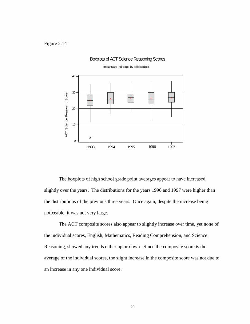
Figure 2.14
The boxplots of high school grade point averages appear to have increased
slightly over the years. The distributions for the years 1996 and 1997 were higher than
the distributions of the previous three years. Once again, despite the increase being
noticeable, it was not very large.
The ACT composite scores also appear to slightly increase over time, yet none of
the individual scores, English, Mathematics, Reading Comprehension, and Science
Reasoning, showed any trends either up or down. Since the composite score is the
average of the individual scores, the slight increase in the composite score was not due to
an increase in any one individual score.
AC
T S
cie
nce
Re
aso
nin
g S
core
0
10
20
30
40
Boxplots of ACT Science Reasoning Scores
(means are indicated by solid circles)
1993 1997199619951994
Page 39
30
Overall it appeared that new freshmen are entering NMT with slightly better
credentials and they are more successful in persisting to the second fall semester. For the
purposes of this study, these trends were not significant enough to divide the data set
according to year and to attempt to build a new predictive model for each year. Instead,
all the data for the different years was combined to provide the learning data set for a
single predictive model.
Page 40
31
3. Methods Used to Construct the Classification Models
3.1 Logistic Regression
The logistic regression model is based upon the assumption that the probability
that an object belongs to a given class follows the logistic distribution. Once this
assumption has been made all that is left to construct the logistic model is to estimate the
parameters using the method of maximum likelihood. The logistic distribution is given
by:
( ) 11|
1 eTi
i iP yβ−
= =+ X
X , (3.1)
where 0 1 1 2 2 ...Ti i i k kx x x= + + + +X β β β β β .
Thus, the likelihood function for the logistic distribution is:
( ) ( )1
ˆ, 1|n
i ii
L P yβ=
= =∏X X
ˆ1
1
1Ti
n
i e β−=
⎛ ⎞= ⎜ ⎟+⎝ ⎠∏ X . (3.2)
The β̂ that produces the maximum likelihood becomes the estimate used in the logistic
model.
In order to make the likelihood function easier to manipulate the natural logarithm
of it is taken. This result is called the log likelihood. Since the natural logarithm is a
monotonically increasing function, the β̂ that produces the maximum log likelihood will
also be the β̂ that produces the maximum likelihood. Therefore, finding the estimates
Page 41
32
for the coefficients for the logistic distribution all boils down to finding β̂ such that
( ){ }ˆlog ,L βX is a maximum. This is found by numerical methods.
Once β̂ is found, the logistic distribution is complete, but the classification rule
that assigns a student to class 1 or class 0 must still be formulated. This rule is found by
determining a “cut-off” probability. Any student whose probability of belonging to class
1 is higher than or equal to the cut-off probability is assigned to class 1, otherwise the
student is assigned to class 0. The value that produced the most overall correct
predictions in the learning sample was chosen to be the cut-off probability. However, if
anyone wanted to raise or lower the number of false positive or false negative
predictions, it can be done by lowering or raising the cut-off probability.
The central difficulty in constructing the logistic regression models in this study
was not estimating β or finding the cut-off probability, but selecting the variables to
enter the model. The goal in variable selection is to find the few key variables that will
give the model the best prediction rates. A model that contains extra variables that are not
helpful at predicting the outcome is likely to be unstable. Instability happens when large
changes occur in the outcome variable due to small changes in the predictor variables.
The variable selection process in this study consisted of several stages.
• First, a univariate analysis was conducted to see which variables alone had significant
relevance to the outcome.
• Next, a stepwise procedure was used to reduce the number of potential candidates for
the final model.
• Next, the variables selected from the stepwise procedure were tested to see if any
interactions existed between them. If there were any interactions, then the
Page 42
33
appropriate interaction term was included as a potential candidate for the final
model.
• Finally, the potential candidates for the final model were carefully examined. Models
with various subgroups of these variables were tested to see which produced the
best prediction rates on the learning sample of data. The simplest model with the
best prediction rate was chosen as the final model.
• Once the final model was chosen, 10-fold cross validation was used to estimate its
true error rate.
In the univariate analysis, a logistic model was built for each predictor variable. The
univariate models were of the form:
0 1( )
1( 1| )
1 jj xP y xe
β β− += =+
, (3.3)
where xj = predictor variable j.
The statistical test used to see if the variable, xj, had any potential predictive ability was
the likelihood ratio test.
The likelihood ratio test in logistic regression is analogous to the partial F test for
linear regression. These tests are used to compare a model’s ability to explain the
outcome with or without a certain set of variables. The notion of a “saturated” model
must be explained in order to understand how the likelihood ratio test works. The
saturated model is the most overfitted model possible since it contains a parameter for
each data point. This model also predicts the outcome variable exactly for each data
point, thus providing a “perfect fit” for these points. The saturated model is useless in
practice since it does not involve the predictor variables. However, it does provide a
standard for which to compare other models. The likelihood ratio test compares the
Page 43
34
likelihood of the model in question to the likelihood of the saturated model. The more
complicated the model, i.e. the more parameters it contains, the larger the model’s
likelihood will become. If the likelihood of the model in question is sufficiently close to
that of the saturated model it may be concluded that the model “fits” the data. A statistic
called deviance, D, is used in the likelihood ratio test. It is calculated as follows:
2 logLikelihood of the current Model
DLikelihood of the Saturated Model
⎡ ⎤= − ⎢ ⎥
⎣ ⎦. (3.4)
Continuing with the univariate analysis, the deviance was used to compare two
models, one containing only the intercept 0β , and the other containing both 0β and 1β .
The change in deviance between these two models was found:
( )0 0 1( ) ,G D Model with only D Model withβ β β= −
( )( )
( )0 10,( )
2 log 2logL Model withL Model with only
L Saturated Model L Saturated Model
β ββ ⎧ ⎫⎡ ⎤ ⎡ ⎤⎪ ⎪= − − −⎨ ⎬⎢ ⎥ ⎢ ⎥⎪ ⎪⎣ ⎦ ⎣ ⎦⎩ ⎭
This expression simplifies to:
( )( )
0 1
0
,2 log
L Model withG
L Model with only
β ββ
⎡ ⎤= − ⎢ ⎥
⎣ ⎦. (3.5)
Under the null hypothesis that 1β equals zero, the statistic, G, has approximately a chi-
square distribution with one degree of freedom [13].
Usually the null hypothesis is rejected if the p-value for the test is less than 0.05,
since low p-values indicate that the data does not support the null hypothesis. However,
Hosmer and Lemeshow recommend including all variables as potential candidates for the
final model if the p-value for the univariate likelihood ratio test is less than 0.25 [9]. This
Page 44
35
ensures that variables that might act as good predictors in conjunction with other
variables are not omitted.
The major shortcoming to univariate analysis is that it does not tell if a group of
variables taken together can provide for correct predictions, although the variables might
not be such good predictors on an individual basis. In order to examine the effects on a
model when more than one variable was involved, a stepwise procedure can be used. This
procedure begins with forward selection and then follows with backward elimination.
Here, the model is first fitted for the intercept only, then each variable is added to the
model and removed to see which most increases the likelihood of the model. Next, the
best candidate for entry is added to the model. This process continues until none of the
variables outside of the model meet the minimum significance level for entry. Also, at
each stage, after a variable enters the model, all the variables within the model are
checked to see if they still meet the statistical requirements to remain in the model. This
variable selection process is based upon statistical criteria only, and it has been known to
select irrelevant variables due to sampling error [9]. This is why it is important to
carefully examine the variables selected from stepwise procedures before constructing the
final model.
During the stepwise procedure a relaxed significance level for entry was used. A
variable could enter the model if its significance level was 0.20 instead of 0.05. This
would usually lead to four or five variables in the model found by the procedure. The
possibility of interactions among these variables was examined. For four variables there
are eleven possible interactions, and for five variables there are twenty-six possible
interactions. Because there were so many possible interactions, only the interactions that
Page 45
36
appeared to be important were tested. The likelihood ratio test was used to see if any
interaction term was statistically significant.
The overall goal was to find a simple model with the best predictive abilities.
Therefore, models consisting of subsets of the final pool of candidates and possible
interaction terms were tested for their ability to correctly classify the outcome on the
learning set of data. The model with the best prediction rate on the learning sample was
chosen as the final model. Unfortunately, the prediction rate on the learning sample
usually overestimates the model’s true predictive ability. In order to get a better estimate,
the prediction rate under 10-fold cross validation was found. This was the final step in
the model building and model assessment process for the logistic regression method.
3.2 Classification and Regression Trees (CART)
CART is a binary recursive partitioning procedure since it splits the objects into
two parts and then continues splitting the resulting parts into two. The way CART
decides to split the objects begins by selecting a predictor variable and then searching
through all the values of that predictor variable in the learning set to find the value that
best separates the objects into two groups. A split is given by a question. If a predictor
variable is ordered then the splits are based upon questions such as: “Does the object
have a value less than or equal to some number for the given predictor variable? “ If the
predictor variable is categorical then the question takes on the form: “Does the object
belong to a specific category (or some subset of categories)?” CART searches through all
the possible splits of all the predictor variables. The one that produces the best split,
where the class heterogeneity of the resulting subgroups is a minimum, becomes the root
Page 46
37
node of the tree. This process is repeated on the resulting subgroups, again allowing all
the predictor variables to be potential candidates for the next split. These splits are
referred to as decision nodes. The tree is grown until the resulting subgroups meet a
minimum class heterogeneity. This becomes the maximum tree. The resulting partition
is a collection of terminal nodes. All the objects in a terminal node are labeled as
belonging to the class that makes up the largest percentage at that node. The percentage
of misclassified objects at a node is called the node impurity. CART is a greedy
algorithm; that is, it only looks at the current best split, not possible combinations of
splits beyond the current one. This allows the algorithm to be fast and efficient at
growing the maximum tree.
The maximum tree is an overfitted model. This tree is very successful at
predicting class outcomes for the learning sample; however, it typically performs very
poorly on an independent set of data or under cross validation. In order to find the best
model, the maximum tree must be pruned back. Sequential levels are removed from the
maximum tree all the way down to the root node. This results in a series of trees, one of
which will provide the best predictions on an independent set of data. Cross validation is
needed to find the optimal tree. The prediction rates for the learning sample give no
indication of which level the pruning should be stopped since they steadily decrease as
the tree is pruned. However, the prediction rates with cross validation start off low with
the maximal tree then begin to increase to a maximum then quickly decrease as the tree
gets pruned down to the root node. The maximum occurs at the optimal tree.
CART software also reports on the various trees in the pruning process. The
optimal tree selected by the software may not always be chosen as the final model. It is
Page 47
38
important to examine any candidate for the final model to see if the splits are logical.
There is always the option of selecting a simpler model if it does not result in too great a
sacrifice of predictive ability.
In the process of growing trees for this study, first all the predictor variables were
allowed to enter the model. The prior probabilities for the outcome classes were also
taken into account. The optimal tree and trees similar to the optimal tree were examined.
Smaller trees with comparable cross validation prediction rates were preferred. Larger
trees however, were carefully examined to see if they produced any revealing information
about the data. Once several trees were examined, one was picked to be the final model
under the guiding principle of simplicity and good predictive ability.
3.3 Discriminant Analysis
Discriminant analysis (DA) was the third classification model used in this study.
Two types of discriminant analysis models were considered, linear and quadratic. DA is
a parametric method that is based upon the assumption that the density functions
associated with the different populations are multivariate normal. Linear discriminant
analysis (LDA) further assumes that the covariance matrices of the different populations
are equal.
There are several ways that a classification rule may be developed in DA. In this
particular study, Statistical Analysis Software (SAS) was used to build the DA model.
This software applies the “largest posterior probability” classification rule [14]. Here, a
new observation is assigned to the class that yields the largest posterior probability. The
Page 48
39
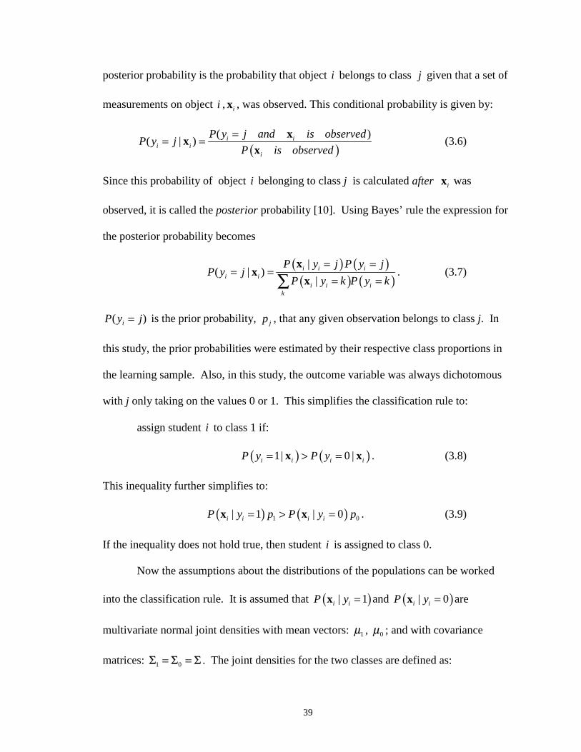
posterior probability is the probability that object i belongs to class j given that a set of
measurements on object i , ix , was observed. This conditional probability is given by:
( )( )
( | ) i ii i
i
P y j and is observedP y j
P is observed
== = xx
x (3.6)
Since this probability of object i belonging to class j is calculated after ix was
observed, it is called the posterior probability [10]. Using Bayes’ rule the expression for
the posterior probability becomes
( ) ( )( ) ( )
|( | )
|i i i
i ii i i
k
P y j P y jP y j
P y k P y k
= == =
= =∑x
xx
. (3.7)
( )iP y j= is the prior probability, jp , that any given observation belongs to class j. In
this study, the prior probabilities were estimated by their respective class proportions in
the learning sample. Also, in this study, the outcome variable was always dichotomous
with j only taking on the values 0 or 1. This simplifies the classification rule to:
assign student i to class 1 if:
( ) ( )1| 0 |i i i iP y P y= > =x x . (3.8)
This inequality further simplifies to:
( ) ( )1 0| 1 | 0i i i iP y p P y p= > =x x . (3.9)
If the inequality does not hold true, then student i is assigned to class 0.
Now the assumptions about the distributions of the populations can be worked
into the classification rule. It is assumed that ( )| 1i iP y =x and ( )| 0i iP y =x are
multivariate normal joint densities with mean vectors: 1μ , 0μ ; and with covariance
matrices: 1 0Σ Σ Σ= = . The joint densities for the two classes are defined as:
Page 49
40
( )( )
( ) ( )122
11 1exp
22p
T
j j jf μ Σ μπ Σ
−⎧ ⎫= − − −⎨ ⎬⎩ ⎭
x x x 0,1j = (3.10)
where p is the number of variables.
With this new information, the classification rule becomes:
assign observation i to class 1 if:
( ) ( )1 1 0 0i if p f p>x x , (3.11)
otherwise assign observation i to class 0.
Substituting equation 3.10 into 3.11 results in:
( ) ( ){ } ( ) ( ){ }1 11 11 1 1 0 0 02 2exp exp
T T
i i i ip pμ Σ μ μ Σ μ− −− − − > − − −x x x x . (3.12)
Since the density functions are assumed to be multivariate normal there are some
intuitive aspects that can be observed from the classification rule. By this assumption,
each population is clustered around its mean, jμ , in the metric space. Also, since the
covariance matrices are assumed equal, the dispersion of each population about its mean
is equal. Therefore, when a new observation comes along, the squared distance of the
new observation to each of the population means is found. The closest population mean
determines the class of the new observation. The squared distance of the observation, ix ,
to the population mean, jμ , is:
( ) ( )1T
i j i jμ Σ μ−− −x x . (3.13)
This expression is sometimes referred to as the Mahalanobis distance [14]. If the prior
probabilities for the different classes are unequal, then they must also be taken into
account when calculating the distance of the new observation to the population means.
Page 50
41
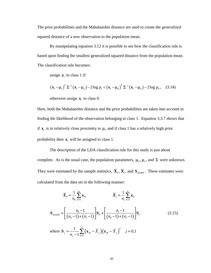
The prior probabilities and the Mahalanobis distance are used to create the generalized
squared distance of a new observation to the population mean.
By manipulating equation 3.12 it is possible to see how the classification rule is
based upon finding the smallest generalized squared distance from the population mean.
The classification rule becomes:
assign ix to class 1 if:
( ) ( ) ( ) ( )1 11 1 1 0 0 02 log 2log
T T
i i i ip pμ Σ μ μ Σ μ− −− − − < − − −x x x x , (3.14)
otherwise assign ix to class 0.
Here, both the Mahalanobis distance and the prior probabilities are taken into account in
finding the likelihood of the observation belonging to class 1. Equation 3.3.7 shows that
if ix is in relatively close proximity to 1μ and if class 1 has a relatively high prior
probability then ix will be assigned to class 1.
The description of the LDA classification rule for this study is just about
complete. As is the usual case, the population parameters, 0μ , 1μ , and Σ were unknown.
They were estimated by the sample statistics, 0X , 1X , and pooledS . These estimates were
calculated from the data set in the following manner:
0X0
010
1
=
= ∑ xn
ikn 1X
1
111
1
=
= ∑ xn
ikn
( ) ( ) ( ) ( )0 1
0 10 1 0 1
1 1
1 1 1 1pooled
n n
n n n n
⎡ ⎤ ⎡ ⎤− −= +⎢ ⎥ ⎢ ⎥− + − − + −⎣ ⎦ ⎣ ⎦S S S (3.15)
where ( )( )1
1
1
jnT
j jk j jk jkj
X Xn =
= − −− ∑S x x 0,1j =
Page 51
42
Finally, the linear discriminant analysis model is complete. Using this model, a
student with predictor variable scores ix is assigned to class 1 if:
( ) ( ) ( ) ( )1 11 1 1 0 0 02 log 2log
T T
i pooled i i pooled iX X p X X p− −− − − < − − −x S x x S x , (3.16)
otherwise the student is assigned to class 0.
In the case where the covariance matrices of the different populations are not
assumed equal, quadratic discriminant analysis (QDA) is used. The fundamental
classification rule, given by equation 3.11, remains the same. The coefficients, 1
2
i
−
Σ ,
however, do not cancel out. Therefore, the classification rule for quadratic discriminant
analysis becomes:
assign student i to class 1 if:
( ) ( ) ( ) ( ) ( ) ( )1 11 1 1 1 1 0 0 0 0 0log 2log log 2log
T T
i i i ip pμ Σ μ Σ μ Σ μ Σ− −− − + − < − − + −x x x x ,
(3.17) otherwise assign student i to class 0.
Here, the generalized distance between the new observation and the population mean
must also take into account the dispersion of the population.
Again, the population parameters were not known so they must be replaced by
their sample estimates. Once this is done, the final quadratic classification rule becomes:
assign student i to class 1 if:
( ) ( ) ( ) ( ) ( ) ( )1 11 1 1 1 1 0 0 0 0 0log 2log log 2log
T T
i i i iX X p X X p− −− − + − < − − + −x S x S x S x S
(3.18)
otherwise assign student i to class 0.
Johnson and Wichern warn that quadratic discriminant analysis is very sensitive
to deviations from normality [10]. Also, Lim, Loh, and Shih found that QDA was one of
Page 52
43
the poorer classification methods in terms of predictive ability [11]. However QDA does
have one positive feature that made it desirable to test its predictive ability in this study.
QDA is not a linear model like LDA and logistic regression. In LDA and logistic
regression the boundaries that separate the classes are flat since they are lines, planes, and
higher-dimension planes. QDA allows for curved boundaries, quadratic functions, to
separate the different populations. In order to see if class boundaries could be curved
instead of flat, QDA models were examined for their predictive ability.
Since DA works under the assumption that the predictor variables are normally
distributed, only continuous predictor variables were allowed to be candidates for entry in
the final model. This restriction on the variables only allowed for High School GPA,
ACT Composite score, and ACT English, Mathematics, Reading Comprehension, and
Science Reasoning Scores to be candidates for the final model. Since there were
relatively few variables to choose from, stepwise methods did not seem necessary. There
were a couple of other reasons for not using stepwise methods. First, stepwise methods
cannot be used with quadratic discriminant analysis . Secondly, Jean Whitaker gave a
scathing review of the use of stepwise methods in discriminant analysis. Whitaker claims
that stepwise methods are unreliable since they capitalize on sampling error and that they
are liable to not select the best subset of predictor variables [15]. Because of these
reasons, stepwise methods were not used to help build the DA model. Instead, models
were built with different subgroups of variables and compared using cross validation.
The following subgroups were used to build both linear and quadratic discriminant
models for the various outcome variables.
Page 53
44
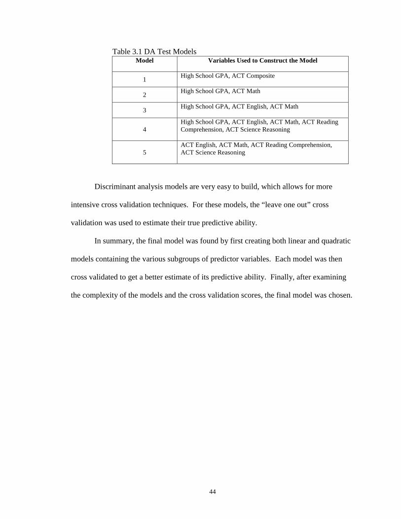
Table 3.1 DA Test ModelsModel Variables Used to Construct the Model
1High School GPA, ACT Composite
2High School GPA, ACT Math
3High School GPA, ACT English, ACT Math
4High School GPA, ACT English, ACT Math, ACT ReadingComprehension, ACT Science Reasoning
5ACT English, ACT Math, ACT Reading Comprehension,ACT Science Reasoning
Discriminant analysis models are very easy to build, which allows for more
intensive cross validation techniques. For these models, the “leave one out” cross
validation was used to estimate their true predictive ability.
In summary, the final model was found by first creating both linear and quadratic
models containing the various subgroups of predictor variables. Each model was then
cross validated to get a better estimate of its predictive ability. Finally, after examining
the complexity of the models and the cross validation scores, the final model was chosen.
Page 54
45
4. Results
4.1.1 Predicting Fall to Fall Persistence with Logistic Regression
Fall to fall persistence was defined as the event of a new freshman enrolling in the
fall semester (or previous summer semester) and still being enrolled for the following fall
term. Of the new freshmen in this study, 71.3% persisted from fall to fall. This is
important to note because any prediction model for fall to fall persistence should have an
overall correct prediction rate greater than 71.3%, otherwise there is no way to tell if the
predictor variables give any information about fall to fall persistence.
Beginning with the univariate analysis for each of the predictor variables, the
following table shows the chi-square statistic and the corresponding p-values of the
likelihood ratio tests for each predictor variable.
Table 4.1 LR Univariate Analysis (First Outcome)
Variable Chi-Square Statistic(1 degree of freedom)
P-Value
1. High School GPA 36.845 .00002. ACT Math Score 26.038 .00003. Pre-Calculus (binary) 21.741 .00004. ACT Science Reasoning Score 10.300 .00135. ACT English Score 8.161 .00436. ACT Reading Comprehension Score
6.400 .0114
7. Major 2.864 .08978. Sex 2.864 .09069. Ethnicity 1.108 .292510. New Mexico High School 0.893 .3447
Due to their high p-values, the variables Ethnicity and New Mexico High School
were excluded from the pool of candidates for the final model. However, there were
significant differences among the scores between the persistors and the non-persistors for
the rest of the variables at the 0.25 significance level.
Page 55
46
The next step in the analysis involved using the stepwise procedure on the
remaining eight variables. Using the relaxed significance level for entry into the model,
α = 0.20, the following variables were selected:
Order of Selection Variable
First High School GPASecond ACT Math ScoreThird Sex
Two interaction terms were next taken into account. These were “Sex*High
School GPA” and “Sex*ACT Math Score.” Both interaction terms were not statistically
significant at the 0.05 level. The p-values for the likelihood ratio tests for these terms
were 0.077 and 0.73 respectively. Hence, no interaction terms were considered.
A preliminary model with the three variables High School GPA, ACT Math Score
and Sex was created. Women were slightly more likely to persist from fall to fall than
men. Of the 288 women in the data set, 75.0% of them persisted, and of the 662 men in
the study, 69.6% of them persisted. However, the most important variables in this model
were High School GPA and ACT Math Score. The p-value for the null hypothesis:
0Sexβ = was 0.1318. At the 0.05 significance level the null hypothesis was accepted and
the variable Sex was dropped without sacrificing a significant amount of variance
explained by the model.
Although the statistical criteria for the model with High School GPA and ACT
Math Score were acceptable, the model was an inadequate predictor. Recall that logistic
regression models the probability that the event occurs. The event in this case was fall to
fall persistence. This probability model was turned into a predictive model by selecting a
cut-off probability. If a student’s probability of persisting from fall to fall was greater
Page 56
47
than the cut-off probability, then that student was labeled as persisting, otherwise he was
labeled as not persisting. The cut-off probability was selected by finding the value that
yielded the greatest overall correct prediction rate. None of the cut-off probabilities
could yield correct predictions for more than 71.3% of the students. This was the exact
proportion of students who persisted from fall to fall in the data set. This correct
prediction rate was achieved by picking a cutoff probability so low that all the students
were labeled as persisting. For example, the cutoff probability for persisting was 0.26. If
a student’s probability of persisting was at least 0.26 then he was labeled as persisting.
However, no student had a probability of persisting lower than 0.26. As the cutoff
probability was raised, the total percentage of correct predictions fell from 71.3% until it
reached 38.7% where everyone was labeled as not persisting. Therefore, fall to fall
persistence could not be adequately modeled using logistic regression.
4.1.2 Predicting Fall to Fall Persistence with CART
At the beginning of the tree growing process, all the predictor variables were
allowed to enter the model. The prior probabilities were specified as 0.713 for class 1,
students who persisted from fall to fall, and 0.287 for class 0, students who did not persist
from fall to fall. These prior probabilities were the respective proportions of the two
classes in the entire data set. At this point the misclassification costs were set equal.
CART grew the maximal tree and found the cross validation prediction rates for
the various pruned levels of the tree. Table 4.2 shows the prediction rates for the
different sized trees.
Page 57
48
Table 4.2 CART Tree Prediction Rates (First Outcome)
Tree NumberNumber of Terminal
Nodes
Cross ValidationOverall CorrectPrediction Rate
Learning SampleOverall CorrectPrediction Rate
1 129 0.632 0.89610 39 0.677 0.82411 37 0.676 0.82112 32 0.676 0.81213 25 0.685 0.79714 18 0.689 0.78215 14 0.696 0.77216 12 0.699 0.76617 10 0.689 0.75918 5 0.690 0.73919 1 0.713 0.713
The optimal tree, tree number 19, had only one node. This indicates that no split
existed that could improve the performance of the tree [6]. The best overall correct
prediction rate, 0.713, occurs when all the students are labeled as persisting from fall to
fall. Given the prediction methods employed by CART and the available predictor
variables, no model could be provided to predict the outcome of fall to fall persistence.
However, a CART model could be produced by varying the misclassification
costs. For example, if the misclassification cost for labeling a student actually in class 0
as belonging to class 1 was increased by 30% over the misclassification cost of the
opposite error, then the optimal tree could predict 26.4% of the non-persistors. Before,
when all the students were labeled as persisting from fall to fall, none of the non-
persistors were identified. This slight improvement lead to a slight decrease in the
model’s ability to predict who will persist and the overall correct prediction rate. Instead
of correctly labeling all of the persistors, 86.4% of them were correctly labeled and the
overall correct prediction rate decreased from 0.713 to 0.692.
Despite the results from the misclassification cost manipulations, fall to fall
persistence could not be adequately modeled by CART using the available predictor
Page 58
49
variables. Forcing the CART method to try predicting only students who did not persist
from fall to fall does not indicate that the predictor variables reveal anything about fall to
fall persistence.
4.1.3 Predicting Fall to Fall Persistence with Discriminant Analysis
Linear and quadratic discriminant models were built in a third attempt to find a
classification model for fall to fall persistence. In view of the fact that logistic regression
techniques failed to provide a model, there was not much hope that linear discriminant
analysis would provide a model either. There was some vague hope however, that
quadratic discriminant analysis might provide some sort of prediction model.
Before the model building process began, the prior probabilities for the two
classes were specified as the class proportions in the learning sample. These were 0.287
for class 0, the students in the data set did not persist from fall to fall, and 0.713 for class
1, the students who did persist from fall to fall. Again, the major test of the model was
seeing if it could predict the correct outcome for more than 71.3% of the students.
The following table shows the models that were tested, the variables included in
each model, and their prediction rates.
Page 59
50
Table 4.3 DA Test Models (First Outcome)
Model Variables
Linear ModelLearningSampleOverallCorrectPredictionRate
Linear ModelCrossValidationOverallCorrectPredictionRate
QuadraticModelLearningSampleOverallCorrectPredictionRate
QuadraticModel CrossValidationOverallCorrectPredictionRate
1High School GPA,ACT Composite
0.704 0.703 0.707 0.703
2High School GPA,ACT Math
0.707 0.705 0.707 0.700
3High School GPA,ACT English, ACTMath
0.707 0.706 0.713 0.708
4
High School GPA,ACT English, Math,ReadingComprehension, andScience Reasoning
0.709 0.706 0.709 0.701
5
ACT English, Math,ReadingComprehension, andScience Reasoning
0.708 0.707 0.707 0.705
None of the cross validation overall correct prediction rates met the requirement
of being greater than 0.713.
Like the logistic model, both the linear and quadratic discriminant analysis
models were only able to achieve an overall correct prediction rate around 0.7 by
classifying nearly all of the students as persisting from fall to fall. There were 273
students in the data set who did not persist from fall to fall, yet none of the DA models
examined ever labeled more than 36 students as belonging to this class.
The third attempt at finding a prediction model for persistence failed. Neither
linear nor quadratic discriminant analysis could produce a model. This was an indication
that neither flat nor curved boundaries exist between the two classes that can be described
using the continuous variables in this study.
Page 60
51
4.2.1 Predicting Fall to Fall Persistence in Good Academic Standing
with Logistic Regression
The second outcome variable was defined as the event of persisting to the second
fall semester with good academic standing versus any other outcome (persisting in poor
academic standing or dropping out). Beginning the variable selection process, the
univariate models were constructed and tested using the log likelihood ratio test. The
results from this analysis are given in Table 4.4.
Table 4.4 LR Univariate Analysis (Second Outcome)Variable Chi-Square
Statistic (1 d.f.)P-Value
1. High School GPA 159.957 .00002. ACT Math Score 69.821 .00003. Pre-Calculus (binary) 56.099 .00004. ACT Composite Score 46.987 .00005. ACT English Score 25.920 .00006. ACT Science Reasoning Score
23.238 .0000
7. ACT Reading Comprehension Score
14.930 .0001
8. Sex (binary) 2.124 .14509. New Mexico High School (binary)
1.945 .1631
10. Ethnicity (binary) 1.711 .190811. Major (binary) 1.162 .2811
It was interesting to note the very large chi-square statistic for High School GPA
in comparison to the statistics for the other variables. The variable Major was eliminated
from further analysis since its p-value was greater than 0.25.
The next step was to build a model using forward selection followed by backward
elimination based upon the ten remaining variables. The variables selected from this
procedure were:
Order of Selection Variable
First High School GPASecond ACT Math Score
Page 61
52
Third New Mexico High SchoolFourth Pre-Calculus
The overall correct prediction rate for this model was 69.3%. Since the
proportion of students persisting in good academic standing in the data set was 54.4%,
the model’s ability to predict the outcome was better than simply assigning all the
students to class 1.
Although all the various ACT scores had significant p-values in the univariate
analysis, there was no need to include them as candidates for the final models since they
were all highly correlated with ACT Math Score. Due to these high correlations, if a
model already contained ACT Math Score, then the other ACT scores would not
contribute any new information about the outcome if they were included. Likewise, the
variable Pre-Calculus was excluded since it was also highly correlated with ACT Math
Score. Although the correlation between Pre-Calculus and ACT Math Score was not as
high as the correlations between the various ACT scores, the inclusion of Pre-Calculus
did not improve the predictive ability of the models tested.
Next, models containing subsets of the variables High School GPA, ACT Math
Score, and New Mexico High School and their interactions were tested. During this
procedure it became evident that High School GPA and ACT Math Score needed to be
included in the final model. The predictive ability of a model was reduced considerably
if it did not contain these two variables. There were two models that produced high
prediction rates on the learning set of data. The first model had a correct prediction rate
of 70.4% and it contained the following two variables:
1. High School GPA
2. ACT Math Score
Page 62
53
The second model had a correct prediction of 70.2% and it contained the following
variables:
1. High School GPA
2. ACT Math Score
3. New Mexico High School
4. High School GPA*New Mexico High School
If a student attended a New Mexico High School, he was slightly more likely to
be in class 1. The percentage of students in the data set who attended a New Mexico
High School and who belonged to class 1 was 56.1%, while the percentage of students
who had not attended a New Mexico High School and who belonged to class 1 was
51.4%. In the second model described above, if a student attended a New Mexico High
School then his likelihood of belonging to class 1 would only increase if he had a high
school GPA greater than 2.83.
The difference in the predictive ability between the two models was negligible
and since the first model was much simpler than the second it was chosen as the final
model. This model was:
( )1 21 2 6.6917 1.4778 0.0765
11| ,
1 x xP y x x
e − −= =+
, (4.1)
where 1x High School GPA= ,
and 2x ACT Math Score= .
Equation 4.1 represents the probability of a student persisting in good academic standing.
The cut-off probability that yielded the most correct predictions overall in the learning
sample was 0.46. Therefore, in order for a student to be labeled as belonging to the
Page 63
54
population of students who persist in good academic standing the student’s probability
must be at least 0.46. This produced the following classification rule:
assign student i to class 1 if:
1 2( 1| , ) 0.46i i iP y x x= ≥ ,
otherwise assign student i to class 0.
In order to get a better estimate of the predictive ability of the final model, 10-fold
cross validation was used. The following table shows the correct and incorrect
classifications produced by the model.
Table 4.5 LR Confusion Matrix (Second Outcome)
Actual Outcome
0 1 Total
0 245 100 345PredictedOutcome
1 188 417 605
Total 433 517 950
The overall correct prediction rate was (245 417) / 950 .697.+ = The proportion of correct
classifications of the students who persisted in good academic standing, or the sensitivity,
was 417 / 517 .807.= The proportion of correct classifications of the students who did
not persist from fall to fall with good academic standing, or the specificity, was
245 / 433 .566= .
The predictive ability of the model may also be examined graphically by plotting
the students’ high school GPA and ACT math score along with the level curve where the
model equals the cut-off probability. Recall that the requirement to be labeled as
belonging to class 1:
1 2( 1| , ) 0.46iP y x x= ≥
Page 64
55
1 2(6.691 1.4778 0.0765 )
10.46
1 x xe− − − ≥+
.
Simplifying this inequality results in:
1 21.4778 0.0765 6.8513x x+ ≥ . (4.2)
This equation provides the requirements on high school GPA and ACT math score
needed for a student to be labeled as persisting in good academic standing. The boundary
line between the two outcomes is:
1 21.4778 0.0765 6.8513x x+ = . (4.3)
A scatter plot of students’ high school GPA and ACT math score that also contains this
boundary line can be used to see how the students are labeled. The following graph is a
scatter plot of only the students who persisted in good academic standing. The points that
lay above the line represent students who were correctly classified.
Figure 4.1
352515
5
4
3
2
ACT Math Score
Hig
h S
choo
l GP
A
with LR Boundary Line (Second Outcome)Students who Persisted in Good Academic Standing
Page 65
56
The bulk of the points lay above the line. This corresponds to the correct classification of
80.7% of the students who persisted in good academic standing.
The ability of the model to correctly classify students who did not persist in good
academic standing was not as good. The following graph is a scatter plot of those
students along with the model.
Figure 4.2
Here the line cuts through nearly the center of the scatter plot. All the points that lay
above the line represent misclassified students. Recall that the correct prediction rate of
students who did not persist in good academic standing was 56.6%. This corresponds to
the percentage of points that lay below the line.
The students who did not persist in good academic standing were a mixed group
of those who left in good academic standing and those who persisted or left in poor
academic standing. This contributed to the high error rate when trying to predict students
who did not persist in good academic standing. The following graph is a scatter plot of
the students who left before their second fall term upon enrollment in good academic
10 20 30
0
1
2
3
4
5
ACT Math Score
Hig
h S
choo
l GP
A
Students who Did Not Persist in Good AcademicStanding and LR Boundary Line (Second Outcome)
Page 66
57
standing. The percentage of students who were mislabeled as persisting in good
academic standing was 56.7%. These incorrect classifications made up 24.2% of the total
misclassifications. It is highly likely that these students left NMT for reasons that were
not due to lack of academic preparation.
Figure 4.3
Of the students who were in poor academic standing at the time they left NMT or
by their second fall semester, only 23.0% were incorrectly labeled as persisting in good
academic standing. Figure 4.4 is a scatter plot of the high school GPA versus ACT math
score of this group of students. Here the bulk of the points, 77.0%, lay below the line.
These students were correctly classified as not persisting in good academic standing.
40302010
4.5
3.5
2.5
ACT Math Score
Hig
h S
choo
l GP
A
and LR Boundary Line (Second Outcome)Students who Left in Good Academic Standing
Page 67
58
Figure 4.4
Now that the strengths and weaknesses of the logistic model have been assessed,
the estimated coefficients in the model must be interpreted. With linear regression the
interpretation of the coefficients in the model is very straightforward. Given the linear
model 0 1y xβ β= + , for every unit change in x there is a change of 1β in y. The
interpretation of the coefficients is not so simple with logistic regression. Here the notion
of odds must be introduced. Odds are defined as:
probability the event occurs
probability the event does not occur.
The odds may be thought of as the likelihood of the event occurring.
The relative likelihood of the event occurring for two different individuals is
found with the odds ratio. Here the event is defined as a student persisting in good
40302010
5
4
3
2
1
0
ACT Math Score
Hig
h S
choo
l GP
A
(Second Outcome)Academic Standing and LR Boundary LineStudents who Left or Persisted in Poor
Page 68
59
academic standing. The odds ratio for a student with a high school GPA 1xΔ points
higher than another student, and controlling for ACT math score is:
1 1 2
1 1 2
1 2
1 2
( 1| , )1 ( 1| , )
( 1| , )1 ( 1| , )
P y x x x
P y x x x
P y x x
P y x x
⎛ ⎞= + Δ⎜ ⎟− = + Δ⎝ ⎠
⎛ ⎞=⎜ ⎟− =⎝ ⎠
.
This expression simplifies to
1 1 1ˆ 1.4778x xe eβ Δ Δ= . (4.4)
A reasonable value for 1xΔ must be chosen. For example, if 1 .5xΔ = then the odds ratio
is 2.09. This indicates that a student who has the same ACT math score, but half a grade
point higher than another student is 2.09 times more likely to persist in good academic
standing.
This same process is used to examine the coefficient on the variable 2x , ACT
math score. Here the odds ratio for two students with the same high school GPA, but one
with 2xΔ points higher on the math portion of the ACT exam, is
2 2 2ˆ 0.0765x xe eβ Δ Δ= . (4.5)
Again, a reasonable value for 2xΔ must be chosen. If 2 5xΔ = points then 0.0765*5e =1.47.
Therefore, for every five points higher a student scores on the math portion of the ACT
math exam, he will raise his likelihood of persisting in good academic standing 1.47
times.
The values 1β̂ and 2β̂ are point estimates of the coefficients 1β and 2β . In order
to gain more information about 1β and 2β , the interval estimates of these values were
Page 69
60
found. According to Hosmer and Lemeshow, the maximum likelihood estimate, ˆiβ , of
the logistic model has approximately a normal distribution with mean, iβ , and standard
deviation, the standard error of ˆiβ [9]. Therefore a 95% confidence interval for iβ is:
ˆ ˆ1.96 ( )i iSEβ β± .
Using this information, the 95% confidence interval for 1β in the model is:
1.4778 1.96*0.1549± ,
(0.298, 2.657) .
Likewise, the 95% confidence interval for 2β in the model is:
0.0765 1.96*0.0185± ,
(0.040,0.113) .
Since neither of these intervals contain zero, it may be concluded with 95% confidence
that 1β and 2β are nonzero.
Confidence intervals for the odds ratios may also be found by exponentiating the
end points of the confidence intervals for the coefficients. The 95% confidence interval
for the odds ratio for the variable High School GPA is:
( )1 10.298 2.657,x xe eΔ Δ,
where 1xΔ is the change in high school GPA. If 1 0.5xΔ = the corresponding 95%
confidence interval for the odds ratio is:
(1.161,3.775) .
Likewise, the 95% confidence interval for the odds ratio for the ACT math score is:
( )2 20.04 0.113,x xe eΔ Δ.
Page 70
61
If 2 5xΔ = , then the confidence interval becomes:
(1.221,1.944) .
Thus, with 95% confidence, if a student achieves half a grade point higher for his high
school GPA, then he is between 1.161 and 3.775 times more likely to persist in good
academic standing. Likewise, if he scores five points higher on the math portion of the
ACT exam, he is between 1.221 and 1.944 times more likely to persist in good academic
standing.
4.2.2 Predicting Fall to Fall Persistence in Good Academic Standing
with CART
Since CART software picks the variables for the model, all the predictor variables
were allowed to be potential candidates. Equal prior probabilities of 0.5 were assigned
to the two outcome classes although 0.54 of the students in the learning set persisted from
fall to fall with good academic standing (class 1) and 0.46 of them did not (class 0). The
difference of 0.04 was not that large. In fact, when prior probabilities of 0.54 and 0.46
were specified, there was no change in the model. Finally, the misclassification costs
were also set equal. There was no greater penalty for mistaking a successful student for
an unsuccessful one or visa versa.
In the pruning process, searching for the optimal tree, the results of several trees
were reported. Table 4.6 shows these results.
Page 71
62
Table 4.6 Cart Tree Prediction Rates (Second Outcome)Tree Number Number of
Terminal NodesCross Validation Overall Correct
Prediction RateLearning Sample Overall Correct
Prediction Rate1 125 0.579 0.887
28 26 0.664 0.77529 25 0.669 0.77330 23 0.679 0.76631 18 0.677 0.74832 8 0.670 0.72233 7 0.664 0.71834 6 0.663 0.71135 5 0.669 0.70936 4 0.677 0.70337 2 0.663 0.683
The pruning process began with the largest tree of 125 terminal nodes and
worked down to the smallest tree with only one terminal node. Normally, as the tree
decreases in size, the cross validation prediction rate goes up to a maximum, indicating
the optimal tree, then the cross validation prediction rate quickly decreases as the tree
becomes very small. However, here there were two relative maximum cross validation
prediction scores. These occurred on tree 30 with 23 terminal nodes and a prediction rate
of 0.679, and tree 36 with 4 terminal nodes and a prediction rate of 0.677. The learning
sample prediction rate behaved in a typical manner, continually decreasing as the number
of terminal nodes decreased.
The tree with 23 terminal nodes was marked as the optimal tree since it had the
best cross validation prediction rate. However, with 23 terminal nodes it was a very big
tree. Figure 4.5 is a thumbnail sketch of this tree. Despite the tree’s cumbersome size
there were some interesting aspects to it. The first two splits were based upon High
School GPA. If a student had a high school GPA less than or equal to 3.105 then he was
classified into group 0, not persisting in good academic standing. Next, if a student had a
high school GPA greater than 3.775 then he was classified into group 1, persisting in
Page 72
63
good academic standing. It was far more difficult to predict the outcomes for students
with high school GPAs between 3.105 and 3.775.
Figure 4.5 Preliminary CART Model (Second Outcome)
As the tree struggled to classify this population, students with high school GPAs
between 3.105 and 3.775, a few splits were made that appear to uphold suspicions about
successful and unsuccessful students at NMT. Looking at the leftmost series of splits
based upon high school GPA and ACT English and Reading Comprehension scores,
these students had low ACT Math scores. If they also had high ACT English scores, the
CART model would assign them to class 0. This seems logical since NMT is a science
and engineering school. There is also evidence in this tree that students with very high
ACT Composite scores, but not equally good high school GPAs do not do well. It has
ACT_RC
ACT_ENG
ACT_RC
ACT_ENG
HS_GPA
ACT_RC
ACT_ENG
ACT_RC
HS_GPA
ACT_RC ACT_SR
ACT_CMP
ACT_CMP
PRECALC
ACT_SR
ACT_RC HS_GPA
ACT_CMP
ACT_CMP
ACT_MATH
HS_GPA
HS_GPA
Page 73
64
been speculated that these students are very talented, but they lack the study skills
necessary for post-secondary work.
Students who start in Pre-Calculus also do not have a high success rate. These
students have a couple of disadvantages. They have not yet mastered the algebra and
trigonometry needed for Calculus and they are set back a semester since Calculus is a
prerequisite or co-requisite for many freshmen courses.
Although the optimal tree had the best overall cross validation prediction score
and some interesting branches, its main disadvantage was its size. The next best tree in
terms of both cross validation prediction rates and size was tree number 36 with only 4
terminal nodes and a cross validation prediction rate of 0.677. Due to this tree’s
simplicity and the fact that its predictive ability was only 0.002 less than the optimal tree,
it was selected as the final CART model. This tree is shown in detail by Figure 4.6.
Since the final model is just the pruned version on the optimal tree it retains the difficulty
of predicting the outcome of students with high school GPAs between 3.105 and 3.775.
This is apparent with the split on the ACT math score. Terminal node 2, which contained
students with high school GPAs between 3.105 and 3.775 and ACT math scores of 22
and below, was a very impure node with only 59.6% of its population being correctly
classified. Likewise terminal node 3, which contained students with ACT math scores
above 22, did not have much of an improvement, with 64.0% of its population being
correctly classified.
Page 74
65
Figure 4.6 Final CART Model (Second Outcome)
Extreme values of high school GPA appear to be a far more definitive than ACT
math score since the correct prediction rates for node 1 and 4 were 71.3% and 82.2%
respectively. However, it is important to remember that these are the prediction rates for
the model using all of the data for the learning sample. If this model was applied to an
independent set of data, its predictive ability would probably decrease.
TerminalNode 1Class = 0
Class Cases %0 221 71.31 89 28.7
N = 310
TerminalNode 2Class = 0
Class Cases %0 59 59.61 40 40.4
N = 99
TerminalNode 3Class = 1
Class Cases %0 112 36.01 199 64.0
N = 311
Node 3Class = 1
ACT_MATH <= 22.500Class Cases %
0 171 41.71 239 58.3
N = 410
TerminalNode 4Class = 1
Class Cases %0 41 17.81 189 82.2
N = 230
Node 2Class = 1
HS_GPA <= 3.775Class Cases %
0 212 33.11 428 66.9
N = 640
Node 1
HS_GPA <= 3.105Class Cases %
0 433 45.61 517 54.4
N = 950
Yes No
Yes No
Yes No
Page 75
66
In order to get a better estimate of the model’s predictive ability, cross validation
was used. Table 4.7 shows the correct and incorrect classifications produced by the
model under cross validation.
Table 4.7 CART Confusion Matrix (Second Outcome)
Actual Outcome
0 1 Total
0 278 152 430PredictedOutcome
1 155 365 520
Total 433 517 950
The overall correct prediction rate, as mentioned before, was (278 365) / 950 0.677+ = .
The sensitivity, or the model’s ability to predict the event of a student persisting in good
academic standing, was 365 / 517 0.706= . The specificity, or the proportion of correct
classifications of the students who did not persist from fall to fall with good academic
standing, was 278 / 433 0.642= .
Another benefit of this simple model is that the prediction rates may be easily
examined graphically. Figure 4.7 is a scatter plot of high school GPA versus ACT math
score along with the model. Only the students who persisted in good academic standing
are shown in this plot. Any points that lay in the regions labeled class 0 are students who
were incorrectly labeled.
Page 76
67
Figure 4.7
Here, the way the model partitions the two variable plane may be observed as
well as where the students’ scores lay on that plane. Figure 4.8 is a scatter plot of the
students who did not persist from fall to fall with good academic standing. These
students either left before their second year or they were not in good academic standing
by the end of their second fall semester. In this plot, the points that lay in regions labeled
class 1 were misclassified.
10 20 30
2
3
4
5
ACT Math Score
Hig
h S
choo
l GP
A
with CART Model (Second Outcome)Students who Persisted in Good Academic Standing
Class1
Class0
Class0
Class1
Page 77
68
Figure 4.8
Many of the students who did not persist in good academic standing had
sufficiently high ACT math scores and high school GPAs to be labeled as successful
students. It would be interesting to see how many of these students either left in poor
academic standing, or persisted with poor academic standing without the students who
left with good academic standing. Figure 4.9 is a scatter plot of this population along
with the model.
10 20 30
0
1
2
3
4
5
ACT Math Score
Hig
h S
cho
ol
GP
A
and CART Model (Second Outcome)Students who Did Not Persist in Good Academic Standing
Class0
Class0
Class1
Class1
Page 78
69
Figure 4.9
Of the students who left in poor academic standing or who persisted in poor
academic standing, 75.1% of them were correctly labeled as belonging to class 0. This
was a fairly high correct classification rate. The same is not true of the students who left
in good academic standing. Of these students, only 34.2% of them were correctly labeled
as belonging in class 0. This means that 65.8% of these students were incorrectly
assigned to group 1. These misclassifications contributed 28.6% of the total error of the
model. Figure 4.10 is a scatter plot of the students who left in good academic standing.
The points that lay in the regions labeled class 1 represent misclassified students.
10 20 30
0
1
2
3
4
5
ACT Math Score
Hig
h S
choo
l GP
A
(Second Outcome)Academic Standing and CART ModelStudents who Left or Persisted in Poor
Class0
Class0
Class1
Class1
Page 79
70
Figure 4.10
The CART model using the two variables, High School GPA and ACT Math
score, was not very successful at predicting the outcome of students who left in good
academic standing. Nevertheless, the CART classification tree does have some
informative aspects. It is logical that students with very good high school GPAs will do
well in post secondary studies and that the opposite is true of students with low high
school GPAs. The classification tree shows this with the first two splits and it helps to
quantify what is a “high” and “low” high school GPA. The model also split the students
with ACT math scores of 22 and less from those with scores of 23 and above. According
to the American College Testing organization, students with ACT math scores in the
range of 20-23 are capable of solving basic, straight forward problems in arithmetic,
probability, algebra, and coordinate geometry [2]. Freshmen at NMT are expected to
solve problems that require several steps and perform complex algebraic manipulations in
302010
4.5
3.5
2.5
ACT Math Score
Hig
h S
choo
l GP
A
and CART Model (Second Outcome)Students who Left in Good Academic Standing
Class1
Class0
Class0
Class1
Page 80
71
first semester Calculus. The described capabilities of students who score in the range
from 20-23 are not sufficient for a first semester Calculus class. In fact, 84.9% of the
students in the data set who scored a 22 or below on the math portion of the ACT exam
began in Pre-Calculus. Not only did this model reveal borderline ACT math scores and
high school GPAs, but it also helps confirm the importance of these two variables as
well.
4.2.3 Predicting Fall to Fall Persistence in Good Academic Standing
with Discriminant Analysis
The logistic regression model worked fairly well at describing the class
boundaries with a linear function. This was an indication that linear discriminant analysis
would perform fairly well too. Nevertheless, quadratic discriminant analysis was tested
to see if it could provide an adequate prediction rule as well.
The model building process began by setting the prior probabilities for the two
classes equal to 0.5. The following table shows the predictive results of the various
models tested.
Page 81
72
Table 4.8 DA Test Models (Second Outcome)
Model Variables
Linear Model:LearningSample OverallCorrectPrediction Rate
LinearModel: CrossValidationOverallCorrectPredictionRate
QuadraticModel :LearningSample OverallCorrectPrediction Rate
QuadraticModel: CrossValidationOverallCorrectPredictionRate
1High School GPA,ACT Composite
0.673 0.669 0.678 0.676
2High School GPA,ACT Math
0.694 0.692 0.691 0.689
3High School GPA,ACT English, ACTMath
0.694 0.693 0.698 0.688
4
High School GPA,ACT English, Math,ReadingComprehension, andScience Reasoning
0.690 0.687 0.690 0.682
5
ACT English, Math,ReadingComprehension, andScience Reasoning
0.6291 0.628 0.632 0.621
Despite the fact that model 3 with the variables High School GPA, ACT English,
and ACT Math had the best overall correct prediction rate, it was not chosen as the final
model. Model 2, with the variables High School GPA, and ACT Math, was the second
best model in terms of overall correct cross validation prediction rate. The difference
between the prediction rates of model 3 and model 2 was only 0.001. This was not a
large enough difference to merit the addition of ACT English into the model. Not only
that, but the coefficient on ACT English in model 3 was negative. This indicated that the
higher a student scores on the English portion of the ACT exam, the less likely he was to
persist in good academic standing. It would not be good to penalize students for having
high scores on their college entrance exams. Therefore, model 2, using linear
discriminant analysis and the two variables High School GPA, and ACT Math was
chosen as the final model.
Page 82
73
The breakdown of how this model performed under cross validation is shown in
the following table.
Table 4.9 DA Confusion Matrix (Second Outcome)
Actual Outcome
0 1 Total
0 293 153 446PredictedOutcome
1 140 364 504
Total 433 517 950
Again, the overall correct prediction rate under cross validation was
(293 364) / 950 0.692+ = . The sensitivity of the model was 364 / 517 0.704= , while the
specificity was 293 / 433 0.677= .
Since this model contains the same variables as the logistic regression model, and
the two models both employ linear functions to separate the populations, the two models
are nearly exactly the same.
The linear discriminant analysis model assigns a student to class 1 if:
1 21.4867 0.0794 6.9620x x+ ≥ ,
1
2
where High School GPA,
and ACT Math Score,
x
x
==
otherwise the student is assigned to class 0.
The logistic regression model assigns a student to class 1 if:
1 21.4779 0.0765 6.8513x x+ ≥ ,
otherwise the student is assigned to class 0.
The specificity of the linear discriminant analysis model was higher than that of
the logistic regression model by 0.111. However, the sensitivity of the linear
Page 83
74
discriminant analysis model was less than that of the logistic regression model by 0.103.
The overall correct prediction rates for the two models differed by 0.005. The similarity
between these two models is further illustrated by the graphs of the boundary lines
between the two classes produced by the models. This is shown in Figure 4.11.
Figure 4.11
The classification rule in linear discriminant analysis was not the only helpful
equation that came out of the analysis. The posterior probability of a student belonging
to class 1 given that he had a high school GPA equal to 1x and an ACT math score equal
to 2x was calculated by:
( ) ( )1 1 1 21 2
1 1 1 2 2 2 1 2
,1| ,
( , ) ( , )
p f x xP y x x
p f x x p f x x= =
+
{ }{ } { }
1 2
1 2 1 2
exp 34.6258 10.6522 1.1856
exp 34.6258 10.6522 1.1856 exp 27.6638 9.1654 1.1061
x x
x x x x
− + +=
− + + + − + +. (4.6)
0 10 20 30 40
3.0
3.5
4.0
4.5
ACT Math Score
Hig
h S
choo
l GP
A
Line1 (LDA Model)
Line 2 (LR Model)
LDA and LR Boundary Lines (Second Outcome)
Page 84
75
With this equation the probability of an individual student belonging to class 1 can be
found. These probabilities can sometimes be more informative than just the predicted
binary outcome.
This model, like the previous models used to predict persistence in good academic
standing, was far more successful at correctly classifying students who left or persisted in
poor academic standing than those who left in good academic standing. Of the students
who left or persisted in poor academic standing, 77.3% of them were correctly labeled as
belonging to class 0, whereas only 44.2% of the students who left in good academic
standing were correctly assigned to class 0. The misclassifications of the students who
left in good academic standing contributed 23.0% of the total errors made by the model.
4.3 Predicting Academic Success
In the process of testing the classification models for fall to fall persistence in
good academic standing, it became apparent that a fair amount of the error involved in
these models was due to labeling students who left in good academic standing as
persisting in good academic standing. It is likely that these students were sufficiently
prepared academically for continuing their studies at NMT. The following table shows
the percentages of students who actually left with good grades but they were
misclassified as persisted with good grades for each of the models.
Page 85
76
Table 4.10 Students who Left in Good Academic Standing
Model
Percentage of Studentswho Left in GoodAcademic Standingwho were Predicted asPersisted in GoodAcademic Standing
Percentage of theErrors ClassifyingClass 0 as Class 1caused byMisclassifying TheseStudents
Percentage of the TotalError Contributed byMisclassifying TheseStudents
Logistic Regression 56.7% 75.5% 24.2%
CART 67.8% 52.9% 28.7%
Linear DiscriminantAnalysis
55.8% 48.3% 23.0%
Another interesting result was the model’s ability to predict the outcomes of
students who made up of the rest of the class 0 population, those who persisted or left in
poor academic standing. Unlike the students who left in good academic standing, most of
the students who either left or persisted in poor academic standing were correctly labeled
by the models. Table 4.11 shows the correct prediction rate of these students.
Table 4.11 Students with Poor Academic Standing
ModelPercentage of Students who Persisted or Leftin Poor Academic Standing who WereCorrectly Classified
Logistic Regression 77.0%
CART 75.1%
Linear Discriminant Analysis 77.3%
These results lead to the creation of a new binary outcome variable that had no
dependence on fall to fall persistence but was only based upon academic outcome. Class
1 consisted of students who either left or persisted in good academic standing and class 0
consisted of students who either left or persisted in poor academic standing. The three
different methods were used to create prediction models for this outcome.
In order for any classification model for the new outcome variables to be valid it
must correctly predict the outcome for more than 67.1% of the students because 67.1% of
Page 86
77
the students in the learning sample belonged to class 1. With this minimum overall
correct prediction rate noted the three models were constructed.
4.3.1 Predicting Academic Success using Logistic Regression
Unlike the other models there is no need to provide a prior probability for logistic
regression. Therefore, the model building process could begin immediately with the
univaritate analysis for each predictor variable. Table 4.12 shows the results from the
univariate analysis. Any predictor variable with a p-value less than 0.25 was allowed to
be a candidate for the final model.
Table 4.12 LR Univariate Analysis (Third Outcome)Variable Chi-Square
Statistic (1 d.f.)P-Value
1. High School GPA 230.446 0.0002. ACT Math Score 81.861 0.0003. Pre-Calculus (binary) 60.211 0.0004. ACT Composite Score 57.108 0.0005. ACT English Score 38.100 0.0006. ACT Science Reasoning Score
23.665 0.000
7. ACT Reading Comprehension Score 19.015 0.000
8. Sex (binary) 3.802 0.0519. New Mexico High School (binary)
2.800 0.094
10. Ethnicity (binary) 1.363 0.24311. Major (binary) 0.002 0.964
All the variables except for New Mexico High School were allowed to be
candidates for the final model. In order to reduce the number of potential candidates the
stepwise method, forward selection followed by backward elimination was used next.
The significance level to enter the model was relaxed to 0.20. The following two
variables were the only ones to meet the 0.20 significance level for entry.
Page 87
78
Order of Selection Variable
First High School GPASecond ACT Math Score
Again, despite their significant p-values in the univariate analysis, the variables
Pre-Calculus and the various ACT scores were excluded as candidates for the final model
due to their high correlation with ACT math score. If an interaction term, High School
GPA*ACT Math Score, was added to the model it increased the overall correct prediction
rate from 0.758 to 0.760. This increase was not large enough to justify including an
interaction term in the model and there was no change in the log likelihood of the model
by including the interaction term at the 0.19 significance level, therefore the variables
chosen for the final model were High School GPA and ACT Math Score.
The overall correct prediction rate for this model on the learning sample was
75.8%. Since this rate is greater than 67.1%, the percentage of students belonging to
class 1 in the learning sample, the predictor variables do give information about the
outcome.
10-fold cross validation as used to get a better estimate of the model’s true
predictive abilities. Table 4.13 shows the correct and incorrect predictions made by the
model under cross validation.
Table 4.13 LR Confusion Matrix (Third Outcome)
Actual Outcome
0 1 Total
0 190 111 301PredictedOutcome
1 123 526 649
Total 313 637 950
Page 88
79
The overall correct prediction rate was (190 526) / 950 0.754+ = . The sensitivity, or the
model’s ability to correctly predict class 1, was 526 / 637 0.826= , while the specificity,
or the model’s ability to correctly predict class 0, was 190 / 313 0.607= .
This final model that represents the probability that a student belongs to class 1 is
given by the following equation:
( )1 21 2 8.0551 2.0819 0.0873
11| ,
1 x xP y x x
e − += =+ , (4.7)
where 1 High School GPAx = , and 2 ACT Math Scorex = .
In order for a student to be labeled as belonging to class 1, his probability of either
persisting or leaving in good academic standing must be equal to or greater than 0.56.
This produces the classification rule:
assign student i to class 1 if:
( )1 21| , 0.58P y x x= ≥ , (4.8)
otherwise assign student i to class 0.
The inequality given by equation 4.8 becomes:
( )1 28.0551 2.0819 0.0873
10.58
1 e x x− + ≥+
,
which further simplifies to:
1 22.0189 0.0873 8.3779x x+ ≥ . (4.9)
Previously, in order for a student to be labeled as persisting from fall to fall in
good academic standing, his high school GPA, 1x , and ACT math score, 2x , needed to be
high enough to satisfy:
1 21.4778 0.0765 6.8513x x+ ≥ .
Page 89
80
These two inequalities represent the class boundaries of the different outcome
variables. These boundaries are graphed together in Figure 4.12 to get a better sense of
how they are oriented in relation to each other.
Figure 4.12
Line 1: Boundary for the Persisted in Good Academic Standing Model(1.4778x1 + 0.0765x2 = 6.8315)
Line 2: Boundary for the Persisted or Left in Good Academic Standing Model(2.0189x1 + 0.0873x2 = 8.3779)
The most notable aspect about the differences between the two plots was that the
boundary line for persisting in good academic standing lies above the boundary line for
either persisting or leaving in good academic standing. This indicates that higher high
school GPA’s and ACT Math scores were needed in order to be labeled as persisting in
good academic standing over either persisting or leaving in good academic standing.
The far less noticeable aspect of these two plots was that line 2 was oriented
slightly more horizontally than line 1. The slope for line 1 was
0.0765 /1.4778 0.0518− = − while the slope for line 2 was 0.0873 / 2.0189 0.0432− = − .
The more horizontal these lines lay, or the closer their slopes are to zero, the less ACT
0 10 20 30 40
3.0
3.5
4.0
ACT Math Score
Hig
h S
choo
l GP
A
Line 1
Line 2
Second Outcome and Third Outcome Boundary Lines
Page 90
81
Math score matters in predicting the outcome relative to High School GPA. Here, ACT
Math score was slightly more important in predicting the outcome of persisting in good
academic standing relative to predicting just good academic standing.
Next, looking at the two groups divided on academic standing only, the boundary
line for this model (line 2) along with a scatter plot of the student data may be examined
to see how the two were related to each other. Figure 4.13 is a scatter plot of the students
who either left or persisted in good academic standing along with their class boundary.
Any points that lay below the line represent the misclassified students.
Figure 4.13
In Figure 4.13, the bulk of the points lay above the line. These correctly classified points
correspond to the 0.826 sensitivity of the model.
Recall that the specificity of the model was 0.607. The model was not as
successful at predicting who would do poorly academically. The following figure is a
scatter plot of the students who either persisted or left in poor academic standing along
0 10 20 30 40
2
3
4
5
ACT Math Score
Hig
h S
choo
l GP
A
and LR Boundary Line (Third Outcome)Students who Persisted or Left in Good Academic Standing
Page 91
82
with the class boundary line. On this graph, any points that lay above the line were
misclassified.
Figure 4.14
Finally, the coefficients of the logistic regression model can be used to reveal how
the likelihood of the outcome changes as the predictor variables change. Referring to
section 4.2.2 the notion of odds ratio will be used again. The odds ratio of a student who
has a high school GPA 1xΔ grade points higher than another student becomes
12.0819 xe Δ. This means the student is 12.0819 xe Δ
times more likely to either persist or
leave in good academic standing, after controlling for ACT math score. If 1xΔ is chosen
to be half a grade point, the odds ratio becomes: 2.0819*0.5 2.83e = . Thus, a student with
half a grade point higher on his high school GPA, but with the same ACT math score as
another student is 2.83 times more likely to belong to class 1.
0 10 20 30 40
0
1
2
3
4
5
ACT Math Score
Hig
h S
choo
l GP
A
and LR Boundary Line (Third Outcome)Students who Persisted or Left in Poor Academic Standing
Page 92
83
Next, looking at ACT math score and controlling for high school GPA, the odds
ratio for a student with a score 2xΔ points higher on the math portion of the ACT exam is
20.0873 xe Δ. Choosing 2 5xΔ = points gives: 0.0873*5 1.55e = . Hence, a student with 5
points higher on his ACT math score, but with the same high school GPA is 1.55 times
more likely to belong to class 1.
Confidence intervals for both the coefficients, 1 2,β β and the their odds ratios can
be found as well. Recall from section 4.2.2 that the 95% confidence interval for iβ is
given by:
( )ˆ ˆ1.96i iSEβ β± ,
where ˆiβ is the maximum likelihood estimator of iβ .
So, the 95% confidence interval for 1β is:
2.0819 1.96 0.1772
(1.7346, 2.4292),
± ∗=
and the 95% confidence interval for 2β is:
( )0.0873 1.96 0.0204
0.0473,0.1273 .
± ∗=
Neither of these two confidence intervals contain zero. Therefore, with 95% confidence,
1β and 2β are significantly different from zero.
Confidence intervals for the odds ratios may be found by exponentiating the
endpoints of the confidence intervals for 1β and 2β . Thus, the 95% confidence interval
for the odds ratio for changes 1xΔ points in high school GPA is:
( )1 21.7346 2.4292,x xe eΔ Δ.
Page 93
84
If 1xΔ is chosen to be half a grade point again, the confidence interval becomes:
( )2.3805,3.3689 .
Likewise, the 95% confidence interval for the odds ratio for changes of 2xΔ points in
ACT math score is:
( )2 20.0473 0.1273,x xe eΔ Δ.
If 2xΔ is chosen to be 5 points again, then the confidence interval becomes:
( )1.2668,1.8898 .
Therefore, with 95% confidence, if a student raises his high school GPA by half a
grade point higher then he is between 2.3805 to 3.3689 times more likely to belong to
class 1. Likewise, if a student raises his score on the math portion of the ACT exam by 5
points then he is between 1.2668 and 1.8898 times more likely to belong to class 1.
4.3.2 Predicting Academic Success using CART
In preparation for growing the classification tree, the prior probabilities for the
classes were set equal to the class proportions in the learning sample; 0.671 for class 1
and 0.329 for class 0. The misclassification costs were set equal so there was no greater
penalty for one error over another.
Table 4.14 shows the results of the pruning process from the maximal tree down
to the root node.
Page 94
85
Table 4.14 CART Tree Prediction Rates (Third Outcome)
Tree NumberNumber ofTerminalNodes
Cross Validation OverallCorrect Prediction Rates
Leaning Sample OverallCorrect Prediction Rates
1 106 0.659 0.9047 67 0.691 0.8778 47 0.698 0.8569 40 0.697 0.846
10 34 0.700 0.83711 22 0.709 0.81512 8 0.730 0.78513 7 0.730 0.78214 4 0.738 0.77215 2 0.718 0.757
The optimal tree chosen by CART was remarkably similar to the final model used
to predict fall to fall persistence in good academic standing. There were the same number
of terminal nodes and the same variables produced the splits, however the splits occurred
at lower values than before. Recall that class 1 represented students who either persisted
or left in good academic standing and class 0 represented students who either persisted or
left in poor academic standing in this model. Figure 4.15 shows the model along with the
learning sample classifications.
Page 95
86
Figure 4.15 Final CART Model (Third Outcome)
Given this model’s optimum cross validation prediction rate and its simplicity, it
was an easy decision to select it as the final model. Since this model’s overall correct
prediction rate was 0.738 this model performs better than assigning all the students to
class 1. The cross validation results for this model are shown in Table 4.15.
TerminalNode 1Class = 0
Class Cases %0 153 68.31 71 31.7
N = 224
TerminalNode 2Class = 0
Class Cases %0 44 59.51 30 40.5
N = 74
TerminalNode 3Class = 1
Class Cases %0 72 27.51 190 72.5
N = 262
Node 3Class = 1
ACTMath<=21.500Class Cases %
0 116 34.51 220 65.5
N = 336
TerminalNode 4Class = 1
Class Cases %0 44 11.31 346 88.7
N = 390
Node 2Class = 1
HSGPA<= 3.525Class Cases %
0 160 22.01 566 78.0
N = 726
Node 1Class = 1
HSGPA<= 2.995Class Cases %
0 313 32.91 637 67.1
N = 950
Yes No
Yes No
Yes No
Page 96
87
Table 4.15 CART Confusion Matrix (Third Outcome)
Actual Outcome
0 1 Total
0 164 100 264PredictedOutcome
1 149 537 686
Total 313 637 950
The model’s overall correct prediction rate under cross validation was
(164 537) / 950 0.738+ = . The sensitivity of the model, or its ability to predict class 1
was 537 / 637 0.843= , and the specificity, or the model’s ability to predict class 0 was
164 / 313 0.524= .
The predictive ability of the model may be examined graphically as well. Figure
4.16 is a scatter plot of the students who persisted from fall to fall in good academic
standing or who left before their third semester. Any points that lay in the regions
labeled class 0 are students who were misclassified.
Figure 4.16
302010
5
4
3
2
ACT Math Score
Hig
h S
cho
ol
GP
A
Standing and CART Model (Third Outcome)Students who Persisted or Left in Good Academic
Class1
Class0
Class0
Class1
Page 97
88
The bulk of the points lay in the regions labeled Class 1. This corresponds to the
sensitivity of 0.843 for the model. The model’s specificity, 0.524, was not as good as the
model’s sensitivity. This becomes apparent with the scatter plot of the students who
persisted or left in poor academic standing. Figure 4.17 shows this scatter plot along with
the CART model.
Figure 4.17
Perhaps the most useful features to CART models are the first two splits on high
school GPA. These two splits divide students into three populations: students who will
not do well academically, students whose academic outcome is difficult to predict, and
students who will do well academically. A substantial percentage of the students, 35.4%,
fall into the category of those whose outcome is difficult to predict. At least the model
tells the range of high school GPAs for these students.
302010
5
4
3
2
1
0
ACT Math Score
Hig
h S
choo
l GP
A
and CART Model (Third Outcome)Students who Persisted or left in Poor Academic Standing
Class1
Class0
Class0
Class1
Page 98
89
4.3.3 Predicting Academic Success with Discriminant Analysis
The DA model building process began by setting the prior probabilities equal to
the class proportions in the learning sample. Following the same procedure as before,
several models containing different subsets of variables were tested for their predictive
ability. Table 4.16 shows the results of the different models.
Table 4.16 DA Test Models (Third Outcome)
Model Variables
Linear Model:LearningSample OverallCorrectPrediction Rate
LinearModel:CrossValidationOverallCorrectPredictionRate
QuadraticModel:LearningSample OverallCorrectPrediction Rate
QuadraticModel:CrossValidationOverallCorrectPredictionRate
1 High School GPA,ACT Composite
0.754 0.750 0.752 0.749
2 High School GPA,ACT Math
0.757 0.757 0.757 0.755
3 High School GPA,ACT English, ACTMath
0.760 0.759 0.759 0.755
4 High School GPA,ACT English,Math, ReadingComprehensionand ScienceReasoning
0.755 0.753 0.753 0.754
5 ACT English,Math ReadingComprehensionand ScienceReasoning
0.695 0.692 0.699 0.694
The linear model with the best overall correct prediction rate contained the
variables: High School GPA, ACT English, and ACT Math. Here the coefficient on the
ACT English score was positive, however it was very small. This coefficient was so
small that 23 ACT English points were worth one ACT Math point. Since ACT scores
range from around 10 to 36, a difference of 23 English points to one math point indicated
that the English score was not contributing much to the model. Despite the slightly
Page 99
90
higher overall correct prediction rate of this model, the variable ACT English was
dropped and the second linear model, with the two variables High School GPA and ACT
Math, was chosen as the final DA model.
The following table shows how the model performed under cross validation.
Table 4.17 DA Confusion Matrix (Second Outcome)
Actual Outcome
0 1 Total
0 153 71 224PredictedOutcome
1 160 566 726
Total 313 637 950
Again, the overall correct prediction rate was (153 566) / 950 0.757+ = . The sensitivity
of the model, or its ability to predict class 1 was 566 / 637 0.889= . The model’s ability
to predict class 0, or the specificity, was 153 / 313 0.489= . By examining these
prediction rates the differences between the two linear models, logistic regression and
linear discriminant analysis appear quite different. The specificity of the LDA model was
0.063 higher than the LR model while the sensitivity of the LDA model was 0.118 lower
than the LR model.
The classification rule according to the LDA model was:
assign student i to class 1 if:
1 22.1082 0.0861 8.2984x x+ ≥ ,
1
2
where High School GPA,
and ACT Math Score,
x
x
==
otherwise assign student i to class 0.
The boundary line between the two classes according to the LDA model was:
1 22.1082 0.0861 8.2984x x+ = ,
Page 100
91
while the boundary line between the two classes according to the logistic regression
model was:
1 22.0189 0.0873 8.3779x x+ = .
The following graph shows the two boundary lines plotted together:
Figure 4.18
Unlike the LDA and LR models produced to predict persistence in good academic
standing, the class boundaries found by these two models do not lie on top of one
another. However that does not necessarily indicate that the two models are different.
By examining the graph, the slopes of the two lines appear nearly equal. Indeed, the
slope for the class boundary of the LDA model was 0.0861/ 2.1082 0.408− = − , while the
slope for class boundary of the DA model was 0.0873 / 2.0189 0.432− = − . The
relationship between ACT math score and high school GPA for the two models are
similar. If the logistic regression model was shifted down so that the cut off probability
403020100
4.0
3.5
3.0
2.5
ACT Math Score
Hig
h S
cho
ol
GP
A
Line 1(LR Model)
Line 2 (LDA Model)
LDA and LR Boundary Lines (Third Outcome)
Page 101
92
for belonging to class 1 was 0.50 instead of 0.58 then the boundary lines for the two
models would appear as follows:
Figure 4.19
This also alludes to the flexibility of the class boundary line. The boundary line
may be shifted vertically to achieve a better prediction of one class over another by
changing the cut-off probability. This change only affects the intercept of the boundary
line, not its slope. For example, if the boundary line is shifted down then high school
GPA and ACT math scores needed to be labeled as belonging to class 1 are also lowered.
Therefore, students who do not meet the “low” standards are definitely liable to not
persist or leave in good academic standing, which in turn raises the model’s specificity.
The same is true of raising the class boundary line. Students who have very good high
school GPAs and ACT math scores probably will continue to do well academically.
403020100
4.0
3.5
3.0
2.5
ACT Math Score
Hig
h S
choo
l GP
A
Line 2 (LDA Model)
Line 1 (LR Model)
LDA and Revised LR Boundary Lines (Third Outcome)
Page 102
93
Therefore, if the class boundary of a model were raised then the sensitivity of the model
would increase accordingly. What made these two models very similar was not the levels
of boundary lines but the slope of the boundary lines. The relative contribution of
predictor variables for each model was nearly the same. That is for the LDA model,
every one point ACT math score was worth 0.0408 point high school GPA, and for the
LR model, every one point ACT math score was worth 0.0432 point high school GPA.
The two models, LR and LDA, achieved similar overall correct cross validation
prediction rates. The overall correct cross validation prediction rate for the LR model
was 0.754, while the overall correct cross validation prediction rate for the LDA model
was 0.757. The differences between these models occurred in their sensitivity and
specificity rates. There were several students who belonged to both class 1 and class 0 in
the middle of the ACT Math Score-High School GPA plane with High School GPA’s
between 3.0 and 3.5 and ACT Scores in the low 20’s. The LR model assigned most of
the people in this range to class 0, thus increasing the model’s specificity. On the other
hand, the LDA model assigned most of the people in the range to class 1 which increased
the models’ specificity.
Finally, looking at the LDA model alone, the formula for the posterior probability
of a student belonging to class 1. This probability is given by:
( ) ( )( ) ( )
1 1 1 21 2
1 1 1 2 0 0 1 2
,1| ,
, ,
p f x xP y x x
p f x x p f x x= =
+
{ }{ } { }
1 2
1 2 1 2
exp 37.0569 11.8224 1.1979
exp 37.0569 11.8224 1.1979 exp 28.7585 9.7142 1.1118
x x
x x x x
− + +=
− + + + − + +. (4.10)
Page 103
94
An alternative but equivalent way to classify a new observation using the LDA
model is to find the posterior probability of the student belonging to class 1 and class 0
and then assign the student the class that yields the largest posterior probability. It is
more informative to have the probability of a student belonging to a given class than a
simple binary prediction. This way it can be seen exactly how likely the student is to
belong to the class to which he was assigned.
Page 104
95
5. GOAL Program
In 1996, NMT began the Group Opportunities for Activities and Learning (GOAL)
program in an effort to improve student retention among new freshmen. The program
was designed to help new freshmen acclimate to living away from home and to provide
these students with extra academic support. In order to participate in the GOAL program,
prospective new freshmen needed to fill out an application and submit an essay
explaining why they wanted to take part in the program. Students who showed this
initiative to join GOAL were accepted. GOAL students lived on the same floor of their
dormitory and they took their core freshmen courses together. This was to help students
form friendships and study groups. The ratio of resident advisors to GOAL students in
the dormitory was raised. These resident advisors were responsible for planning social
activities as well as helping form study sessions and looking out for students who might
be having academic problems so that the struggling student could be offered extra help
early on. The GOAL students were also required to take a special class to help them
improve their study habits, learn time management skills, and to introduce them to
resources on the campus.
In recent years there has been some inquiry about the effectiveness of the GOAL
program. Has it truly helped the students who participated in it? This is particularly
difficult to determine since the participants in the program were self-selected. However,
with the classification models it is possible to predict how well the GOAL students would
be expected to do given their high school GPA and ACT math scores and compare the
prediction to how well they actually performed.
Page 105
96
Since the purpose of the GOAL program was to retain students and to help them do
well academically, the logistic model used to predict persistence in good academic
standing was chosen to estimate these students probability of belonging to class 1. In
order to make the comparison of how well the students actually performed versus how
well they were predicted to perform, first the logistic model was used to find the
individual probabilities of each student persisting in good academic standing based upon
their high school GPA and ACT math score. These probabilities were calculated using
equation 4.1. The total number of students predicted as belonging to class 1 in the GOAL
group was the sum of the individual probabilities. This predicted number of students
persisting in good academic standing was compared to the actual number of those who
belonged to this class.
There were two years of GOAL students in the data set, 1996 and 1997. The results
for these two years were very different. In 1996, the first year of the GOAL program, 53
students participated and only 20 actually persisted in good academic standing.
However, given the credentials of the group as a whole and using the logistic model,
26.59 of these students were predicted as persisting in good academic standing.
On the other hand, the 1997 GOAL students did better than what was expected of
them. That year, 56 students participated in the program and 36 persisted in good
academic standing. According to the logistic model, 32.69 of the students were predicted
as persisting in good academic standing.
The actual performance of these students was examined to see if their good and bad
results were statistically significant. There is no theoretical distribution for the class
assignment process of these students. Therefore, the natural variation of the assignment
Page 106
97
process was examined by simulation. In the simulation, each student’s probability of
persisting in good academic standing was compared to a Uniform(0,1) random number.
If the probability was higher than the number generated then the student was assigned to
class 1; otherwise he was assigned to class 0. Uniform(0,1) random numbers vary
uniformly between zero and one, as the name implies. Therefore, if a student has a high
probability of belonging to class 1 then the uniform random number generated is likely to
be lower than the student’s probability, which would cause the student to be assigned to
class 1. The opposite is true of students with low probabilities of belonging to class 1.
By assigning students to class 1 in this manner, we can find confidence limits on the total
number of students expected to belong to class 1 for the two groups of GOAL students.
After 1000 iterations counting the number of 1996 GOAL students assigned to class 1
by simulation, the 5th and the 95th percentile were (21, 32). Since the interval does not
contain 20, it can be concluded that the 1996 GOAL students did do worse than expected
at the 90% confidence level since 90% of the data fall between the 5th and 95th percentile.
The performance of the 1997 GOAL students was not that easily determined. After 1000
iterations counting the number of 1997 GOAL students assigned to class 1 by
simulation, the 5th and 95th percentile were (27, 38). There were 36 students who
belonged to class 1 in the 1997 GOAL program. The performance of this group is close
to being significantly better than expected.
The first year of GOAL students did not do well, but it is unclear if GOAL students
in following years did better than was predicted of them. It would be very beneficial to
examine the 1998 and 1999 GOAL participants to see if they performance was
Page 107
98
significantly better than expected. Otherwise no conclusions can be made about the
GOAL program yet.
Page 108
99
6. Conclusions
Catching the waves of enthusiasm about improving freshmen retention, this study
began with many lofty goals: to find the model that could predict the elusive outcome of
fall to fall persistence, to gain insight on the factors that lead to students’ academic
success and what might influence them to remain at NMT or leave, and to find a clear
answer to the question about the GOAL program’s effectiveness. Unfortunately, none of
these objectives were truly realized. Nevertheless, other smaller discoveries were made
in this extensive model building process. The failure to find a prediction model of fall to
fall persistence lead to a more careful examination of the predictor variables and the
outcome variable. Fortunately, the dependent variables were effective at predicting
academic outcome. The models did a fairly good job at predicting fall to fall persistence
in good academic standing and they were even more successful at predicting academic
success, whether a student persisted or left in good academic standing. The academic
outcome models also presented the best variables at predicting academic outcome, High
School GPA and ACT Math Score. It was already known that high school GPA was
more important than ACT scores in determining a student’s academic outcome, but with
the models it is possible to quantify this importance. Finally, the real barrier to finding an
answer about the GOAL program’s effectiveness is just a matter of collecting more data,
which can be done easily in the future.
After the failure to find a model to predict fall to fall persistence, it became very
clear that none of the available predictor variables gave any information about what
might cause students to remain enrolled at NMT. At first, it appeared as though fall to
Page 109
100
fall persistence could be modeled since the univariate analysis of the predictor variables
showed that several variables were statistically relevant to the outcome on Table 4.1.
Unfortunately, their statistical relevance probably came from the fact that most of the
students persisting from fall to fall did so in good academic standing. Later on, it became
evident that the students who persisted in good academic standing were quite different
from the rest of the population, enough so that their outcome could be adequately
predicted. In hindsight, these variables, such as high school GPA, college entrance exam
scores, ethnicity, sex, and the scant first semester variables do not indicate anything about
a student’s motivation to attend NMT. The failure to find a prediction model for fall to
fall persistence, however, may not be entirely dependent on the limited information
provided by the predictor variables.
The outcome variable fall to fall persistence does not appear to be a very
worthwhile indicator of a student going on to complete of a four-year degree. Clifford
Adelman dropped the persistence variables from his study of bachelor degree attainment
due to weak architecture. Adelman found that there was an enormous range in how far
along students were to completing their degrees in the time from the students’ first year
of college to their second year [3].
This problem of having a very mixed population of students who completed three
semesters cropped up here too. Looking at the new freshmen who entered in fall or
summer semesters from 1993-1995, 25.5% of these students who persisted from fall to
fall persisted in poor academic standing. It was interesting to see what happened to these
students a little further on in their academic careers at NMT. The persistence rates of the
freshmen who remained enrolled to their second fall semester were examined after four
Page 110
101
more semesters, which should, theoretically, land them near the middle of their senior
year. Of the students who persisted to their second fall semester in poor academic
standing, 41.9% went on to complete four more semesters, while 80.4% of the students
who persisted to their second fall semester in good academic standing went on to
complete four more semesters. This result indicates that fall to fall persistence alone was
not a good indicator of freshmen remaining enrolled until their 7th semester, which should
be close to graduation.
The student populations at the end of the third semester were not so mixed when
they were separated based upon academic standing. The independent variables, High
School GPA and ACT math score, were capable of differentiating the second and third
outcome variables, persistence in good academic standing versus any other outcome and
either persistence or withdrawal in good academic standing versus any other outcome.
This indicates that the high school GPAs and ACT math scores of the students who
belonged to class 1 of the two outcome variables, were substantially different from those
that belonged to class 0. Although High School GPA and ACT Math Score were the best
predictor variables, there were other variables that had significantly different means for
the two classes. This was shown in the univariate analysis in Tables 4.4 and 4.12. The
univariate logistic regression analysis is equivalent to performing two sample t-tests for
continuous data or chi-square tests for discrete data [9]. Tables 4.4 and 4.12 show that
the variables that had significantly different means or cell counts at the 0.05 level were
High School GPA, all the various ACT scores, and Pre-Calculus. These variables were
not included in the final models due to their correlation with ACT Math Score. None of
the other variables had significantly different means at the 0.05 level. However, the
Page 111
102
variable Sex, for the third outcome variable, persistence or withdrawal in good academic
standing, was barely not significant with a p-value of 0.051.
In order to see how the means of these variables differed between the classes for
the second and third outcome classes, Table 6.1 is a list of the variables along with their
class means and standard deviations.
Examining the mean and standard deviation of the different classes can give a
little more insight into the importance of High School GPA and ACT Math Score. The
mean indicates the location where the data points are centered, while the standard
deviation measures the spread of the data. In general, around 95% of the data lay within
two standard deviations of the mean. In order for a variable to be a good predictor, the
mean values for class 1 and class 0 of the variable must be quite different, enough so that
it is certain that the differences are not due to random variation. A way to get a rough
estimate whether the predictor variables show some differences between the classes is to
examine how much the class means differ and if the difference is large in comparison
with the standard deviation of the two classes. Taking both outcome variables into
account, the difference between the mean high school GPA for the two classes is around
half a point, and the class variances are also around half a point. This is the best ratio of
mean difference to standard deviation among all the variables, which also explains High
School GPA’s status as the most important predictor variable. The next best ratio occurs
with the variable ACT Math Score. Here, the mean differences are around two points
and the class standard deviations are around four points. The largest class separation
appeared in these two variables. Table 6.1 helps to show the individual potential of the
Page 112
103
variables’ predictive ability, however the models themselves give more information how
High School GPA and ACT Math score can work together in predicting class outcome.
Table 6.1 Second Outcome Class and Third Outcome Class StatisticsSecond Outcome:Class 1: Persistence inGood Academic Standing;
Class 0: any otheroutcome
Third Outcome:Class 1: Persistence orWithdrawal in Good Academicstanding;
Class 0: Persistence orWithdrawal in Poor AcademicStanding
Variable
Class 0 Class 1 Class 0 Class 1
Overall
Mean 3.104 3.544 2.970 3.527 3.343HighSchoolGPA St Dev 0.554 0.473 0.524 0.474 0.556
Mean 24.300 26.573 23.789 26.396 25.537ACTMathScore St Dev 4.169 4.015 4.217 3.979 4.238
Mean 25.069 26.692 24.677 26.579 25.953ACTComposite
St Dev 3.672 3.512 3.719 3.487 3.674
Mean 23.734 25.097 23.300 25.053 24.476ACTEnglish
St Dev 4.066 4.019 4.126 4.016 4.133
Mean 26.152 27.429 25.805 27.410 26.881ACTReadingComp. St Dev 5.429 5.186 5.407 5.226 5.337
Mean 25.568 26.890 25.339 26.753 26.287ACTScienceReason. St Dev 4.156 4.212 4.054 4.249 4.236
Mean 0.547 0.308 0.594 0.330 0.417Pre-Calculus(binary) St Dev --- --- --- --- ---
Mean 0.279 0.323 0.256 0.327 0.303Sex(binary)
St Dev --- --- --- --- ---
Mean 0.707 0.745 0.687 0.747 0.727Ethnicity(binary)
St Dev --- --- --- --- ---
Mean 0.626 0.669 0.649 0.650 0.649NM HighSchool(binary) St Dev --- --- --- --- ---
Mean 0.852 0.876 0.847 0.874 0.865Major(binary)
St Dev --- --- --- --- ---
-Coding for the binary variables;Pre-Calculus: 1 if a student took a Pre-Calculus first semester,
0 if a student took a Calculus or higher course first semesterSex: 1 if female, 0 if maleEthnicity: 1 if Caucasian, 0 Everyone elseNM High School: 1 if attended a NM High School, 0 otherwiseMajor: 1 if declared major the first semester, 0 if undeclared major the first semester
Page 113
104
In growing the CART tree the first three most definitive splits occurred on high
school GPA and ACT math score. The CART model also revealed how the outcomes of
students with very high or very low high school GPAs were easy to predict, and the
model gave estimates of these “high” and “low” GPAs. The model also showed that
ACT Math Score was the best variable to try to separate the two classes in the very mixed
population that have high school GPAs somewhere between 3.0 and 3.6.
One of the benefits of the LR and LDA models was that the relationship between
high school GPA and ACT math score could be examined. The slope of the class
boundary lines of the model is the conversion factors of ACT Math to High School GPA.
One whole high school GPA point is quite large, since high school GPA normally ranges
from 2.0 to 4.0, so instead one quarter of a high School GPA point was used in
comparison to one ACT Math point. Table 6.2 shows the number of ACT math points
needed to be equivalent to one quarter of a high school GPA point along with how much
one ACT math point is worth in terms of high school GPA.
6.2 High School GPA and ACT Math Score14 High School GPA point is
worth X ACT Math points1 ACT Math point is worth Y
High School GPA pointsModel
X YLR used to Predict Persistence inGood Academic Standing
4.83 0.0518
LDA used to Predict Persistencein Good Academic Standing
4.68 0.0534
LR used to Predict Persistence orWithdrawal in Good AcademicStanding
5.78 0.0432
LDA used to Predict Persistenceor Withdrawal in Good AcademicStanding
6.12 0.0408
Approximately five points on the math portion of the ACT exam are worth one
quarter of a point High School GPA. According to designers of the ACT exam a
Page 114
105
difference of five points is worth a significant amount. The math portion of the exam is
organized into sections of four points, 16-19, 20-23,…,33-36. The test is designed so that
the math abilities can be easily assessed given the section where the student’s score fell.
The difference between abilities of a student who scores in one section lower than
another is substantial [2]. Since the sections are in four point intervals, if two students
have a difference of five points then their scores lay in two different intervals, possibly
separated by an interval. This implies that their math abilities are considerably different.
The coefficients in the models were reported to four decimal points. This does
not help to find an easy-to-remember prediction rule. However, if the coefficients were
rounded to one digit then the LR and LDA models become equivalent. This becomes
apparent after scaling the coefficient on High School GPA to equal 2. The LR and LDA
class boundary lines once this scaling has been done are shown below. (Again High
School GPA 1x= and ACT Math Score 2x= .)
Fall to Fall Persistence in Good Academic Standing:
LR: 1 22 0.1035 9.2723x x+ =
LDA: 1 22 0.1068 9.3657x x+ =
Good Academic Standing:
LR: 1 22 0.0865 8.2995x x+ =
LDA: 1 22 0.0853 8.2236x x+ =
If the coefficients for these lines were rounded to the nearest digit then the boundary line
for determining fall to fall persistence in good academic standing would be:
11 2102 9x x+ = ,
and the boundary line for determining good academic standing would be:
Page 115
106
11 2102 8x x+ = .
The prediction rates of these two class boundary lines can be examined with the learning
set of data. Table 6.3 shows how well the line 11 2102 9x x+ = separated students who
persisted in good academic standing versus everyone else. The classification rule
assigned students to class 1 if 11 2102 9x x+ ≥ , otherwise they were assigned to class 0.
Class 1 consists of students who persisted in good academic standing and class 0 contains
everyone else.
Table 6.3 Confusion Matrix for Rounded Coefficient Model (Second Outcome)
Actual Outcome
0 1 Total
0 274 126 400PredictedOutcome
1 159 391 550
Total 433 517 950
This model with rounded coefficients worked fairly well on the data set with an overall
correct prediction rate of (274 391) / 950 0.70+ = , a sensitivity of 391/ 517 0.76= , and a
specificity of 274 / 433 0.63= .
Table 6.4 show the predictive ability of the classification rule that labels a student
as either persisting or leaving in good academic standing if 11 2102 8x x+ ≥ , otherwise the
student is labeled as either leaving or persisting with poor academic standing.
Page 116
107
Table 6.4 Confusion Matrix for Rounded Coefficient Model (Third Outcome)
Actual Outcome
0 1 Total
0 124 48 172PredictedOutcome
1 189 589 778
Total 313 637 950
This model had an overall correct prediction rate of (124 589) / 950 0.75+ = , a sensitivity
of 589 / 637 0.92= and as specificity of 124 / 313 0.40= . This model labeled most
students as persisting or leaving in good academic standing which caused the sensitivity
to be much higher than the specificity. The prediction rates of these two models with
rounded coefficients were reported in case someone wanted to use them in the future.
Finally, the models in this study can be used as a tool in assessing the
effectiveness of freshmen programs at NMT. The models predict how well the students
in the freshmen programs ought to do given their background, which can be compared to
how well they actually did. Then simulation can be used to see if the difference in the
predicted and actual outcome is statistically significant.
In summary, there were several main conclusions that have come out of this
study. First, either very different variables are needed to predict fall to fall persistence or
some other measure of persistence must be used in order to find a student retention
model. Although persistence alone could not be predicted, high school GPA and ACT
math score can be used to predict academic outcome. Not surprisingly, High School
GPA was the most important predictor of post secondary academic outcome among these
freshmen. Finally, the models did estimate how important high school GPA was to the
outcomes and they also revealed how high school GPA relates to ACT math score.
Page 117
108
References
[1] ACT Inc. 2000. ACT Assessment: Test Preparation: Content Areas of the ACT Tests.
(http://www.act.org/aap/testprep/index.html), [July 19, 2000].
[2] ACT Inc. 2000. PLAN/ACT Standards for Transition: What Your Score Really
Means. (http://www.act.org/standard/planact/scores.html), [July 19, 2000].
[3] Adelman, Clifford. 1999. Answers in the Tool Box: Academic Intensity, Attendance
Patterns, and Bachelor’s Degree Attainment. Washington, DC:U.S. Department of
Education. (http://www.ed.gov/pubs/Toolbox/index.html), [July 19,2000]
[4] Ali, Hamdi F., Abdulrazzk Charbaji and Nada Kassim Hajj. 1992. A Discriminant
Function Model for Admission at Undergraduate University Level, International
Review of Education, 38, 505-518.
[5] Breiman, Leo, Jerome Friedman, Richard Olshen and Charles Stone. 1984.
Classification and Regression Trees, Chapman and Hall, New York.
[6] Stienberg, Dan and Phillip Colla. 1995. CART: Tree-Structured Non-Parametric
Data Analysis. Salford Systems, San Diego, California.
[7] Council of University Presidents. 1999. Performance and Effectiveness Report of
New Mexico Universities.
(http://www.unm.edu/~cup/pep99/PEP/Full%20Report.PDF), [July 19, 2000].
[8] Dey, Eric L. and Alexander W. Astin. 1993. Statistical Alternatives for Studying
College Student Retention: A Comparative Analysis of Logit, Probit, and Linear
Regression, Research in Higher Education, 34, 569-581.
[9] Hosmer, David W. and Stanley Lemeshow. 1989. Applied Logistic Regression,
John Wiley and Sons, New York.
[10] Johnson, Richard A. and Dean W.Wichern. 1998. Applied Multivariate Statistical
Analysis, Prentice Hall, Upper Saddle River, New Jersey.
[11] Lim, Tjen-Sien, Wei-Yin Loh and Yu-Shan Shih. 1999. A Comparison of
Prediction Accuracy, Complexity, and Training Time of Thirty-three Old and New
Page 118
109
Classification Algorithms, Department of Statistics, University of Wisconson,
Madison,
(http://www.stat.wisc.edu/p/stat/ftp/pub/loh/treeprogs/quest1.7/mach1317.pdf), [July 20, 1999].
[12] Meshbane, Alice and John D. Morris. 1996. Predictive Discriminant Analysis Vs.
Logistic Regression in Two-Group Classification Problems, Eric Document ED 400 280.
[13] Myers, Raymond H. 1990. Classical and Modern Regression with Applications,
Duxbury Press, Belmont, California.
[14] SAS Institute Inc. 1990. SAS/STAT User’s Guide, Version 6, Volume 1. SAS
Institute Inc., Cary, North Carolina.
[15] Whitaker, Jean S. 1997. Use of Stepwise Methodology in Discriminant Analysis
Eric Document ED 406 447.
Page 119
110
Appendix A. Logistic Regression Cut-Off Probabilities
The logistic regression model allows for changes in the number of false positive
and false negative predictions by altering the cut-off probability. The following two
tables report various cut-off probabilities and the resulting overall correct prediction rate,
sensitivity, specificity, false positive rate and false negative rate on the learning sample.
The overall correct prediction rate is the number of the correct predictions divided by the
total number of predictions. The sensitivity is the number of students correctly assigned
to class 1 divided by the total number of students who actually belong to class 1. The
specificity is the number of students correctly assigned to class 0 divided by the total
number of students who actually belong to class 0. The false positive rate is the number
of students incorrectly assigned to class 1 divided by the sum of students incorrectly and
correctly assigned to class 1. Finally, the false negative rate is the number of students
incorrectly assigned to class 0 divided by the sum of students incorrectly and correctly
assigned to class 0.
Table A.1 Logistic Regression Model for Predicting Fall to Fall Persistence in Good Academic Standing
Cut-OffProbability
OverallCorrect
Sensitivity Specificity False Positive False Negative
0.38 67.1 89.2 40.6 35.8 24.10.40 67.6 87.4 43.9 35.0 25.50.42 68.7 85.7 48.5 33.5 26.10.44 69.4 83.8 52.2 32.3 27.10.46 70.4 82.6 55.9 30.9 27.10.48 70.1 79.3 59.1 30.2 29.50.50 70.0 76.0 62.8 29.1 31.30.52 69.5 73.1 65.1 28.5 33.00.54 69.2 70.4 67.7 27.8 34.3
Page 120
111
Table A.2 Logistic Regression Model for Predicting Good Academic StandingCut-Off
ProbabilityOverallCorrect
Sensitivity Specificity False Positive False Negative
0.50 75.6 88.7 48.9 22.1 32.00.52 75.4 87.3 51.4 21.5 33.50.54 75.4 85.1 55.9 20.3 35.20.56 75.8 84.1 58.8 19.4 35.40.58 75.8 82.5 62.0 18.5 36.40.60 75.4 81.3 63.6 18.1 37.40.62 74.8 78.8 66.8 17.2 39.20.64 74.3 76.9 69.0 16.6 40.50.66 72.9 73.3 72.2 15.7 42.9
Page 121
112
Appendix B. Results Using a Reduced Data Set from Raising the Minimum High School Grade Point Average
The current admission requirements for new freshmen entering New Mexico Tech
include having at least a 2.5 high school GPA and at least a score of 21 on the ACT
Composite. The minimum high school GPA was recently raised from a 2.0 to a 2.5. The
changes to this new student population have not been observed yet. With the models and
the data set, it is possible to estimate the outcome of students who meet the current
admission requirements, but who do not meet the requirements to be labeled as belonging
to class 1 for the second and third outcome variables.
In the data set, 822 of the students met the current admission requirements. Of
these students, 325 were classified as not persisting in good academic standing according
to the logistic regression classification rule given by Equation 4.2. In this group of 325,
62.5% actually did not persist in good academic standing. Using the CART model
described by Figure 4.6, 354 students were classified as not persisting in good academic
standing. In this new group, 67.5% were correctly classified.
For the third outcome variable, class 0 consisted of students who either left in
poor academic standing or persisted in poor academic standing. Using the logistic
regression classification rule for the third outcome variable, Equation 4.9, 196 students
who meet the current admission requirements were assigned to class 0. Of these students,
60.2% were correctly classified. Finally the CART model described by Figure 4.15 was
used and 220 students were assigned to class 0. Here, the outcome of 64.0% of the 220
students was correctly predicted.