Predicting Urban Growth on the Atlantic Coast Using an Integrative Spatial Modeling Approach Jeffery S. Allen and Kang Shou Lu Clemson University Strom Thurmond Institute Coastal Community Workshop, March 30, 2006, Ridgeland, SC
Transcript
Predicting Urban Growth on the Atlantic Coast Using an Integrative Spatial
Modeling Approach
Jeffery S. Allen and Kang Shou LuClemson University
Strom Thurmond Institute
Coastal Community Workshop, March 30, 2006, Ridgeland, SC
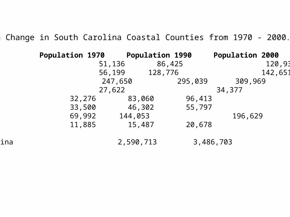
Population Change in South Carolina Coastal Counties from 1970 - 2000.
County Population 1970 Population 1990 Population 2000Beaufort 51,136 86,425 120,937Berkeley 56,199 128,776 142,651Charleston 247,650 295,039 309,969Colleton 27,622 34,377 38,264Dorchester 32,276 83,060 96,413Georgetown 33,500 46,302 55,797Horry 69,992 144,053 196,629Jasper 11,885 15,487 20,678
South Carolina 2,590,713 3,486,703 4,012,012
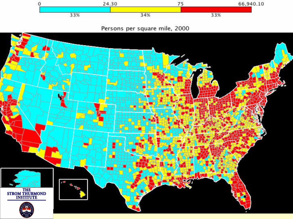
Population density map for North Carolina, South Carolina, and Georgia
# of People Per Square Mile*
> 800
400 - 800
200 - 400
100 - 200
0 - 100
* 1999 population estimates by CACI International, Inc. based on 1990 US Census
5.3%
30.2%
0%5%
10%15%20%25%30%35%
South Carolina: Comparison of Population Growth to Increase in Developed Land 1992-97
Developed Land
Population
Source: (London and Hill, 2000) -- USDA, US Census Bureau and Jim Self Center on the Future, Clemson University.
Total Acres of Land Conversion by State, 1992-1997 (thousand acres) Rank STATE Acres converted to developed land (1,000 acres)1 Texas 1219.5 2 Pennsylvania 1123.23 Georgia 1053.24 Florida 945.35 North Carolina 781.56 California 694.87 Tennessee 611.68 Michigan 550.89 South Carolina 539.710 Ohio 521.2
Source: (London and Hill, 2000) -- USDA, 1997 National ResourceInventory Summary Report
Location of Study Area
Urban Growth Trends (Past)
1985-1997
Urban Area Grows by 67%
1985-2000
Population Grows by 20.6%
Sprawl Index 3 : 1(ratio of urban area growth to population growth)
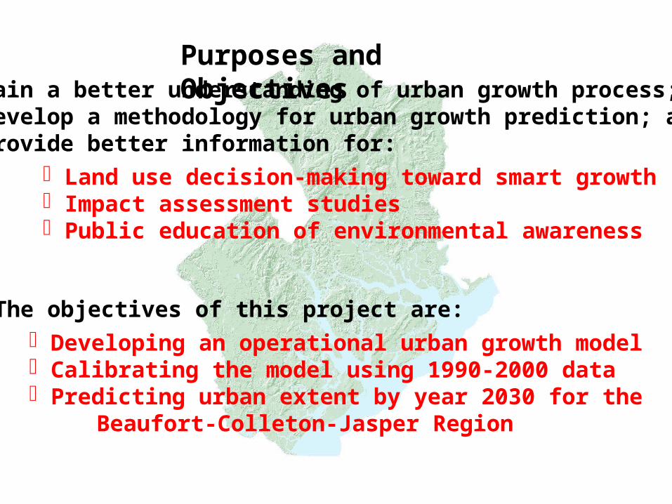
Purposes and ObjectivesGain a better understanding of urban growth process; Develop a methodology for urban growth prediction; andProvide better information for:
Land use decision-making toward smart growth Impact assessment studies Public education of environmental awareness
Developing an operational urban growth model Calibrating the model using 1990-2000 data Predicting urban extent by year 2030 for the Beaufort-Colleton-Jasper Region
The objectives of this project are:
Urban Growth Models
Lowry’s Model (1957) and Its Variants Cellular Automata (Deltron) Model (San Francisco Bay Area)
--- Clarke (1996) California Urban Future Model (CUF I and II) --- Landis (1994, 1995, and 1997) Land Transformation Model (LTM) (Michigan’s Saginaw Bay Watershed)
---Pijanowski et al (1997)
1. Components or structures of the land use systems:simple vs. complex2. Relationships between components, agents, factors, and processes:
deterministic vs. indeterministic.3. Changes over space (and time): ordered vs. random vs. chaotic4. Spatial distribution or patterns: regularity vs. irregularity (fractal)
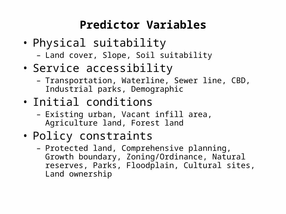
Zoning/Ordinance, Natural reserves, Parks, Floodplain, Cultural sites, Land ownership
Data Sources
Land-use (SCDNR)
Population Density(Census)
Elevation(USGS)
Soil Suitability(NRCS)
Reach Files, Version 3(USEPA)
Subwatersheds(SCDNR)
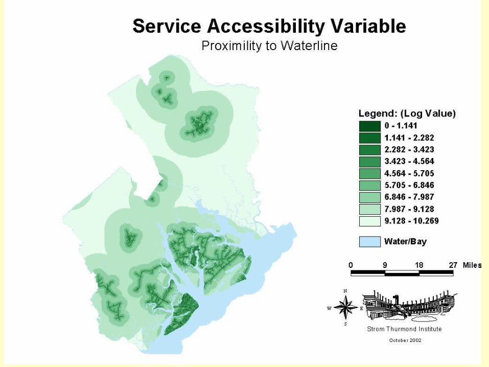
Examples of Predictor Variables
Distance to 2000 Urban Area
Distance to 80 Industry Point
Distance to Roads
Distance to Highway System
Distance to Water Lines
Distance to Sewage system
Final Suitability
Census
Soils
Distance to Existing Development
Final Study Area Selection
Final Suitability
Most Suitable234Least Suitable
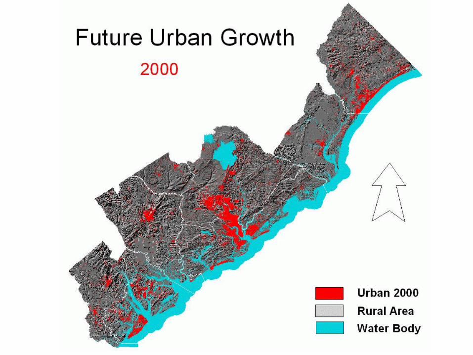
Results---Predicted Urban GrowthBCJ Region
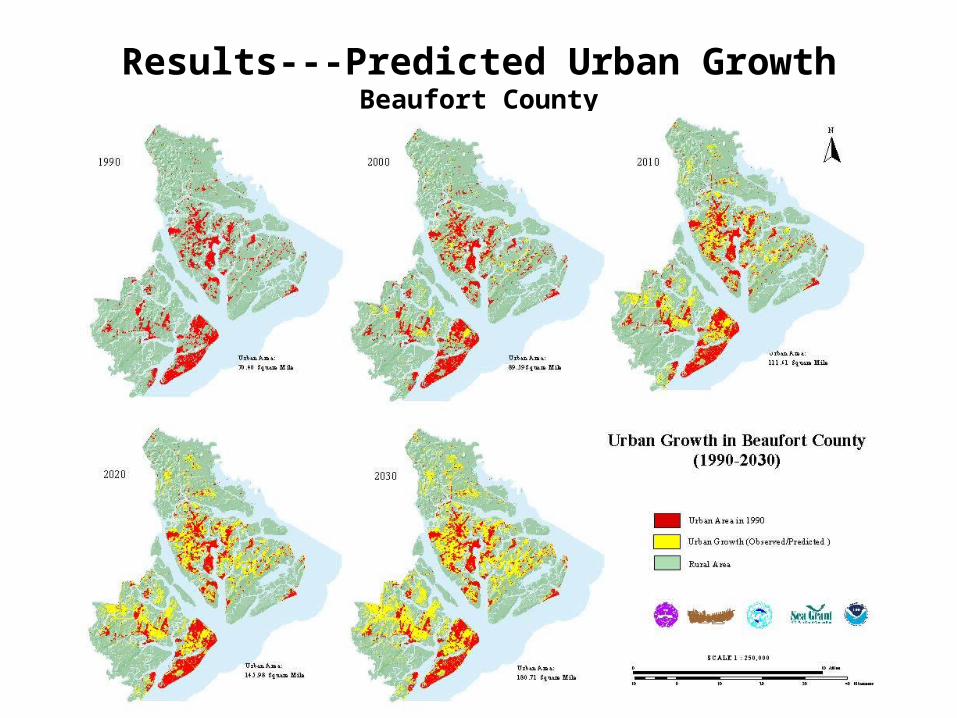
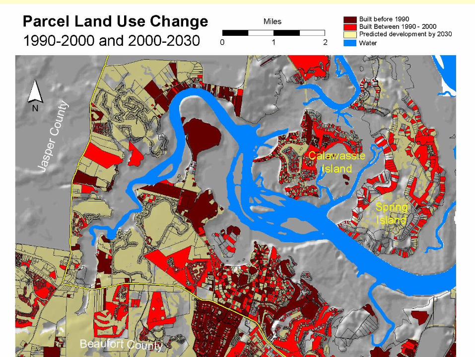
Results---Predicted Urban GrowthBeaufort County
Beaufort County Growth Simulation
Growth Ratio 3:1
Estimated Habitat Losses for Selected Species (1990-2030) Area (in acres) Habitat Loss
Common Name 1990 2030 Acres %
Green Treefrog 301323.57 243374.81 57948.76 19.23 Red Fox 68338.83 41023.59 27315.24 39.97 Red Cockaded Woodpecker (Endangered) 20882.65 17984.84 2897.81 13.88 Wood Stork (Endangered) 135728.03 128129.46 7598.57 5.60
Note: Urban development through 2030 was predicted based on the current growth ratio.
Simulated Growth
Urban Sprawl Problems
Urban growth is necessary and unavoidable. But uncontrolled growth - urban sprawl results in many problems such as:
Increased cost of living Rising taxes and pressure on infrastructure and urban services Traffic congestion and increased (travel) time Environmental pollution Loss of farm/forest land, habitats and rural (natural) landscape Downtown declines and community segregation
Benefits of Urban Growth
Increased standard of living Generation of wealth Increase in amenities Production of affordable housing Increase in tax base New business opportunities New job opportunities Increased “freedom” with the automobile It is what we desire - “Freedom of Choice”
Urban Growth Trends
The pattern follows paths of subsidy.
•Undervalued infrastructure
•Discounted resources
•Reductions for individual risk
•Unintended consequences of past policies
What do we do now?
Growth is coming whether we want it or not Determine where we do not want to grow Increase communication among SPD’s, etc. Be inclusive in planning Provide incentives for growth in “growth areas” Provide “dis-incentives” for areas to protect Make users pay the freight for new growth It is always easier said than done!!!