+ All Categories
Home > Documents > PREDICTING WATER QUALITY BY RELATING SECCHI DISK ...

PREDICTING WATER QUALITY BY RELATING SECCHI DISK ...

Date post: 26-Oct-2021
Category:
Upload: others
View: 1 times
Download: 0 times
Share this document with a friend
44
PREDICTING WATER QUALITY BY RELATING SECCHI DISK TRANSPARENCY DEPTHS TO LANDSAT 8 Miranda J. Hancock Submitted to the faculty of the University Graduate School in partial fulfillment of the requirements for the degree Master of Science in the Department of Geography, Indiana University August 2015
Transcript

PREDICTING WATER QUALITY BY RELATING SECCHI DISK

TRANSPARENCY DEPTHS TO LANDSAT 8

Miranda J. Hancock

Submitted to the faculty of the University Graduate School

in partial fulfillment of the requirements

for the degree

Master of Science

in the Department of Geography,

Indiana University

August 2015

ii

Accepted by the Graduate Faculty, Indiana University, in partial

fulfillment of the requirements for the degree of Master of Science.

Master’s Thesis Committee

Vijay O. Lulla, Ph.D , Chair

Daniel P. Johnson, Ph.D.

Frederick L. Bein, Ph.D.

iii

ACKNOWLEDGEMENTS

I would like to thank the professors and staff of the Geography department; their

knowledge and guidance has made this process a positive, enjoyable experience. I would like to

specifically thank my Graduate Advisor, Vijay Lulla. Vijay’s expertise, enthusiasm, and guidance

helped to make the completion of this thesis possible.

I would like to thank my good friend, Chris Duvall, for offering up his boat to use for data

collection at Brookville Reservoir. This project would not have gone as smoothly without his

kindness. I would like to thank my sister, Hannah, for the numerous peer reviews she has

provided over the last few years. She was always available to help, despite her busy schedule,

and it has been greatly appreciated.

A final, special thank you goes to my husband Marc. His support, encouragement, and

patience have been instrumental to my success. I am incredibly excited to be completing this

project, and I cannot adequately express how grateful I am to Marc for his advice and support.

iv

Miranda J. Hancock

PREDICTING WATER QUALITY BY RELATING SECCHI DISK TRANSPARENCY

DEPTHS TO LANDSAT 8

Monitoring lake quality remotely offers an economically feasible approach as opposed

to in-situ field data collection. Researchers have demonstrated that lake clarity can be

successfully monitored through the analysis of remote sensing. Evaluating satellite imagery, as a

means of water quality detection, offers a practical way to assess lake clarity across large areas,

enabling researchers to conduct comparisons on a large spatial scale. Landsat data offers free

access to frequent and recurring satellite images. This allows researchers the ability to make

temporal comparisons regarding lake water quality. Lake water quality is related to turbidity

which is associated with clarity. Lake clarity is a strong indicator of lake health and overall water

quality. The possibility of detecting and monitoring lake clarity using Landsat8 mean brightness

values is discussed in this report. Lake clarity is analyzed in three different reservoirs for this

study; Brookeville, Geist, and Eagle Creek. In-situ measurements obtained from Brookeville

Reservoir were used to calibrate reflectance from Landsat 8’s Operational Land Imager (OLI)

satellite. Results indicated a correlation between turbidity and brightness values, which are

highly correlated in algal dominated lakes.

Vijay O Lulla, Ph.D., Chair

v

TABLE OF CONTENTS

List of Tables .................................................................................................................................... ii

List of Figures .................................................................................................................................. iii

Introduction ..................................................................................................................................... 1

Background ...................................................................................................................................... 5

Remote Sensing and Water Quality ........................................................................................ 5

Landsat .................................................................................................................................... 7

Secchi Disk Transparency and Landsat .................................................................................. 11

Study Area ...................................................................................................................................... 13

Methods ......................................................................................................................................... 15

Field Data Collection .................................................................................................................. 15

Satellite Data ............................................................................................................................. 19

Utilizing Satellite Imagery to Estimate SDT ............................................................................... 21

Water Only Image ...................................................................................................................... 21

Area of Interest (AOI) Creation (Brookville Lake) ...................................................................... 22

Geist and Eagle Creek Reservoirs AOIs ...................................................................................... 24

Results ............................................................................................................................................ 25

Regression Equations and Tests of Significance ........................................................................ 25

Conclusions .................................................................................................................................... 31

References ..................................................................................................................................... 33

Curriculum Vitae

vi

LIST OF TABLES

Table 1: EPA Status of Brookville, Geist, and Eagle Creek Reservoirs in Central Indiana ................ 2

Table 2: Landsat 8 Band Designations ............................................................................................. 9

Table 3: SDT Sample Locations and SDT Depths ............................................................................ 18

Table 4: Pixel Size vs Accuracy ....................................................................................................... 21

Table 5: Brookville AOIs ................................................................................................................. 23

Table 6: Band Combinations Trials................................................................................................. 25

Table 7: Regression Data................................................................................................................ 26

Table 8: Final Model ....................................................................................................................... 27

Table 9: Predicted vs. Actual SDT ................................................................................................... 27

Table 10: Predicted SDT values for Eagle Creek and Geist Reservoirs........................................... 28

vii

LIST OF FIGURES

Figure 1: Timeline of Landsat Missions ............................................................................................ 7

Figure 2: Study Area ....................................................................................................................... 13

Figure 3: SDT Sample Locations ..................................................................................................... 17

Figure 4: Landsat 8 Study Image .................................................................................................... 20

Figure 5: Unsupervised Classification map of Geist reservoir used as a guide to differentiate

vegetation and other classes when selecting AOIs. ....................................................................... 22

Figure 6: AOI Selection of Eagle Creek ........................................................................................... 24

Figure 7: Predicted SDT Map for Eagle Creek Reservoir ................................................................ 29

Figure 8: Predicted SDT Map for Geist Reservoir .......................................................................... 30

1

Introduction

As lake clarity and turbidity are one in the same for the scope of this study, it is

important to understand turbidity. Turbidity measures the degree at which water loses its

transparency due to the presence of suspended particulates. The higher the level of suspended

particulates, including algae, the murkier the water.

Algae are commonly found in Indiana lakes and streams. A moderate concentration of

algae is necessary for biologically productive, healthy lakes. However, excessive concentrations

of algae can be linked to some adverse health effects and higher levels of waterbody turbidity.

Excessive concentrations of algae negatively impact the ecological balance of lakes in the form

of diminished recreations use, fish kill, and possible contamination of drinking water supplies.

The water bodies examined in this paper, Brookeville Reservoir, Eagle Creek Reservoir, and Geist

Reservoir have experienced regular seasonal algal blooms (Indiana Department of

Environmental Management , 2015).

Factors promoting algal blooms stem from a combination of physical and chemical

factors including available nutrients, temperature, sunlight, turbidity, hydrology, pH and salinity.

The exact combination of factors that cause and support an algal bloom is not well understood

and it is not possible to contribute blooms to a specific factor or combination of factors (Center

for Earth and Environmental Science, 2015; Schlacher, Lloyd, & Wiegand, 2010). Eagle Creek

and Geist reservoirs are on the Federal Clean Water Act list of impaired water bodies. Water

bodies are placed on this list when they are considered too polluted or otherwise degraded and

unable to meet water quality standards set by their governing authorities. The two reservoirs

are on this list due, in part, to high Chlorophyll-a (algae) concentrations. (Table 1). Brookville

reservoir is on the impaired water bodies list due to polychlorinated biphenyls (PCBs) in fish

2

tissue. PCBs are not directly related to algal blooms, however Brookville reservoir has algae

bloom issues and the reservoir is being closely watched by state and federal environmental

agencies.

Globally, algae blooms are an increasing problem in all types of waterbodies due to

rising water temperatures, increases in atmospheric carbon dioxide concentrations, and changes

in rainfall patterns, to name a few (United States Environmental Protection Agency, 2013).

Nutrients, as mentioned above, are recognized as one of the most notorious promoters and

supporters of algae growth. Nutrients, in the form of phosphorus and nitrogen, permeate

through waterbodies internally and externally. External nutrient sources come from runoff and

soil erosion of fertilized lawns and fields, deforested areas and sewage effluent. Internal

nutrient sources consist of phosphates that attach to sediments in the waterbody.

Nutrient rich water contains low levels of oxygen availability and as such promote

sediments to release those attached phosphates into the water thus encouraging the growth of

algae. Without productivity and dissolved oxygen, the waterbody is unable to support beneficial

and necessary organisms (Center for Earth and Environmental Science, 2015). Measuring lake

clarity is an important part of evaluating algae levels and lake water quality. For example, Lake

Table 1: EPA Status of Brookville, Geist, and Eagle Creek Reservoirs in Central Indiana

Retrieved from http://ofmpub.epa.gov/waters10/attains_index.control

3

Erie has shown signs of yearly blooms during summer months since 2008 according to the

National Center for Coastal Ocean Science. (Wynne, 2013)

Because of legislation and citizen concern, a water sampling program has been

undertaken by the Indiana Department of Environmental Management (IDEM), the Indiana

Department of Natural Resources (DNR), the Indiana State Department of Health (ISDH), and the

Board of Animal Health (BOAH). Each year, these organizations work to study, monitor, and

sample algal blooms in Indiana lakes. For the 2014 sampling season, IDEM sampled for blue-

green algae and processed those samples according to type and quantity of blue-green algae, as

well as for microcystin, sylindrospermopsin, and anatoxin-a, toxins associated with blue-green

algae.

Indiana uses the World Health Organization (WHO) guideline level of 100,000 cells/ml or

microcystin toxin level of 6 parts per billion (ppb) to indicate a high cell count advisory. Beaches

in Indiana close if the microcystin toxin level reaches 20ppb for a waterbody. Indiana uses the

guideline of 5ppb of cylindrospermopsin and 80 ppb of anatoxin-a for a high cell count advisory.

Citizens are notified via various media outlets if toxins reach threshold levels. This compilation

of state-collected water quality data provides an opportunity to evaluate Indiana lakes and keep

lake users safe and informed. For the 2014 sampling year, the IDEM reported a high cell count

for Brookville Reservoir on August 19, 2014. High cell counts were also reported for Geist and

Eagle Creek Reservoirs on August 26, 2014 (Indiana Department of Environmental Management

, 2015).

This study of water quality data focuses on using remotely sensed satellite data to

monitor inland lake quality. Satellites have been shown to provide a greater amount of spatial

information at an improved cost compared to spot sampling programs like those administered

4

by state organizations described above. Satellite-based measurements may provide a

mechanism for early detection of blooms and/or the detection of hot-spots in unsampled or

unreachable locations (Kloiber, Brezonik, Olmanson, & Bauer, 2002).

5

Background

Remote Sensing and Water Quality

Landsat imagery has been used for remote sensing of water quality (Brezonik,Menken,

& Bauer, 2005; Fuller & Minnerick, 2001-2006). Previous studies have also shown that water

clarity and Landsat data have an established relationship (Kloiber, Brezonik, Olmanson, & Bauer,

2002; Tebbs, Remediios, & Harper, 2013; Bonansea, Rodriguez, Pinotti, & Ferrero, 2014).

Kloiber et al. (2002) identify similar results between secchi disk transparency (SDT) depth and

Landsat data due to the underlying physical basis and the spectroradiometer’s ability to collect

hyperspectral reflectance data. Likewise, researchers have acknowledged that spectral features

of lakes are consistently related to optically active substances including suspended sediment

which contributes to turbidity (Jensen J. R., 1983). The spectral features that are of upmost

interest to this study stem from sources that make-up total radiance (Lt). Total Radiance is

recorded by Landsat 8 as a function of electromagnetic energy of four sources, whereas Lt = Lp +

Ls + Lv + Lb (Jensen J. R., 2007). Lv deals with a portion of radiance from the downwelling of solar

and sky radiation that penetrates the air-water interface and interacts with the water and

organic/inorganic constituents, like algae, and then exits the water column without

encountering the waterbody floor (Jensen J. R., 2007). The radiance information captured here

can then be transformed to brightness temperatures or values and, as a result, provide valuable

information about the organic/inorganic matter contained within the waterbody. When the

main goal of a study is to identify or provide information about organic/inorganic matter in the

water column, it is important to avoid the Lb source of radiation. Lb is the portion of radiation

that infiltrates the air-water network and reaches the bottom of the water body and then moves

back up through the water body to then exit the water column. Radiance from this source (Lb)

or from the bottom of a water body makes characterizing the water column above the bottom

6

difficult (Jensen J. R., 2007). Due to the Lb source of radiation Olmansen et al. (2002) recommend

collecting samples in water that is 15 feet or deeper.

Estimating turbidity via Landsat data has limitations that must be taken into

consideration. Remote sensing of lakes has been known to be problematic as lakes are different

in terms of the surrounding land use, ecology and water chemistry (Olmanson, Kloiber, Bauer, &

Brezonik, 2001; Tebbs, Remedios, & Harper, 2013). Studies have identified a number of satellite

sensors like MODIS, MERIS, SeaWiFS, MASTER and more that have been used to quantitatively

monitor lake water quality (Tebbs, Remediios, & Harper, 2013; Kudela, et al., 2015). In this

study, a high spatial resolution is necessary as the study area lakes are small (about 2 km

across). Due to the small lake size Landsat 8’s Operational Land Imager (OLI) was chosen

because it posseses a high spatial resolution of 30 meters in the visible, near-infrared, and short-

wave infrared bands. The high resolution allows for better detection of small scale spatial

variability across the lakes of interest. Similarly, the OLI predeccessor (ETM+) was chosen for

these same reasons as in the study by Tebbs et al.,2013.

The satellite sensor, in this case Landsat 8, must be able to relate a characteristic of the

waterbody to an “inherent optical property” in order to extract brightness values (Brezonik,

Menken, & Bauer, 2005). In this study, the characteristic is SDT and the “inherent optical

property” is the radiance measured by Landsat 8 within the spectral bands of interest.

Estimation limitations or errors may arise from atmospheric conditions through incoming solar

radiation penetrating the water surface and then leaving the water column then reaching the

satellite sensor. The intensity of solar radiations varies by latitude, season, time of day, and

weather conditions. Because atmospheric conditions, sensor response, and incoming irradiance

change with time it is not recommended to compare asynchronous Landsat data with in situ

measurements (Brezonik, Menken, & Bauer, 2005).

7

Landsat The Landsat Missions began in 1972 with Landsat 1 and have continued through to the

current operation of Landsat 8 (Figure 2).

Figure 1: Timeline of Landsat Missions

Retrieved from http://www.USGS.gov

On February 11, 2013, Landsat 8 launched from Vandenberg Air Force Base, California.

The Landsat 8 satellite is different from previous Landsat missions as it carries two push-broom

instruments, the Operational Land Imager (OLI) and the Thermal Infrared Sensor (TIRS). The OLI

sensor is similar to Landsat 7’s Enhanced Thematic Mapper Plus (ETM+) except that the OLI

sensor has two additional spectral bands (U.S. Geological Survery, 2015) . As this study works to

apply satellite imagery to regional assessment of lake clarity using Operational Land Imager (OLI)

bands found within Landsat 8, it also works to create a better understanding of Landsat 8’s

capabilities through water quality monitoring using OLI’s spectrally narrower bands. Landsat 8

bands 3 and 4 have been used with success in this study. Band 4 (red) has been improved to a

narrower wavelength (0.64 - 0.67) and is designed for improved sensitivity to discriminate

vegetation slopes. Previously in Landsat 7, the red band had a wider wavelength (0.63 - 0.69)

and was not as sensitive to vegetation slopes. Slope-based vegetation indices are a combination

of visible red and near infrared. This combination indicates a state of abundance of vegetation

cover and biomass (Roy, et al., 2014). Band 3 (green) has been improved to a wavelength of

8

0.53-0.59. This band is useful in assessing plant vigor. Plant vigor is expressed through algal

blooms via phosphorus or nitrogen loading.

As Sriwongsitanon, Surakit, & Thianpopirug (2011) explain, there is no standard

prediction equation for water quality parameters for images collected on different dates for the

same location. Conversely, prediction models are getting close on a standardized model for

images contemporaneously taken with field samples. This study will utilize Landsat 8 band 3

and band 4 to further validate the possibility that water quality monitoring through satellite

imagery can be a standardized process.

OLI has a deep blue visible channel (band 2) that is designed specifically for water

resources and coastal zone analysis as well as an infrared channel (band 9) that can be utilized

for the detection of cirrus clouds. The TIRS sensor collects two spectral bands (bands 10 and 11)

for the wavelength previously covered by one band (band 6) on Landsat 7. The Landsat 8

sensors provide seasonal coverage at a spatial resolution of 30 meters (visible, NIR, SWIR); 100

meters (thermal); and 15 meters (panchromatic). (Landsat Science, 2014) Landsat 8 provides

significant improvement in data quality and radiometric quantization than in previous Landsat

sensors. Landsat 8 radiometric quantization is 12-bits whereas the Thematic Mapper (TM) and

ETM+ is 8-bits. Landsat 8 data is collected and archived every 16 days. However, cloud cover on

acquisition dates may result in a lower frequency of useable data.

Landsat 8 has eight OLI, 30 meter spatial resolution, multispectral bands (Figure 4): (1)

Coastal; 0.43 - 0.45 µm; (2) Blue 0.45 - 0.51 µm; (3) Green 0.53 - 0.59 µm; (4) Red0.64 - 0.67 µm;

(5) NIR 0.85 - 0.88 µm; (6) SWIR1 1.57 – 1.65 µm; (7) SWIR2 2.11 – 2.29 µm; and, (9) Cirrus 1.36

– 1.38 µm. Landsat 8 also has one OLI panchromatic band, 15 meter spatial resolution: (8) 0.50 -

0.68 µm and two, 100 meter spatial resolution TIRS bands: (10) TIRS1 10.6 – 11.19 µm and (11)

9

TIRS2 11.5-12.51 µm. The two TIRS bands are resampled to 30 meters to match the OLI

multispectral bands. Landsat 8 data is delivered as “.tar.gz” compressed files via HTTP

Download. Each file is approximately 1GB (compressed) and 2GB (uncompressed). As this study

utilizes landsat 8 bands (3) 0.53 – 0.59 µm and (4) 0.64 – 0.67 µm other studies have also found

success when using these ranges to estimate turbidity. (Brezonik, Menken, & Bauer, Landsat-

based Remote Sensing of Lake Water Quality Characteristics, Including Chlorophyll and Colored

Dissolved Organic Matter (CDOM), 2005). Landsat 8 bands 5-11 provide measures of radiance in

the mid-and thermal-infrared regions and have not shown use when trying to estimate water

characteristics like SDT, chlorophyll, or turbidity (Brezonik, Menken, & Bauer, Landsat-based

Remote Sensing of Lake Water Quality Characteristics, Including Chlorophyll and Colored

Dissolved Organic Matter (CDOM), 2005).

Table 2: Landsat 8 Band Designations

Retrieved from http://www.USGS.gov

10

For this study, OLI spectral bands have been chosen because they are narrower than the

ETM+ (Landsat 7) bands and have the ability to avoid atmospheric absorption features. As

mentioned above, the 15 meter and 30 meter resolution of the OLI sensors gives researchers a

chance, for the first time, to access the world’s lakes at a high spatial resolution and positional

accuracy. The OLI bands have been designed to incorporate technical advancements that

improve performance over the previous Landsat sensors (Roy, et al., 2014). One significant

change from Landsat 7 to Landsat 8 is that the OLI sensors are pushbroom with focal planes

aligning long arrays of detectors across-track. Previous Landsat instruments used whisk-broom

sensors.

Some of the benefits to using pushbroom sensors include less pixel distortion, longer

dwelling time, narrow swath width, simple mechanical system, and a complex optical system.

The whiskbroom sensors operate with pixel distortion, shorter dwelling time, and wider swath

width to name a few. Pushbroom sensors offer improved geometric fidelity, radiometric

resolution, and signal-to-noise characteristics compared to the whiskbroom sensors.

In addition to the upgraded pushbroom sensors, Landsat 8 OLI bands operate with a

high or very specific signal-to-noise ratio (SNR). A high SNR is an important factor for water

constituent mapping because of the very low signal that water generates. The low signal

creates the variations in water quality to be lost in the noise of lower or less specific SNR

systems. Previous Landsat instruments have limited capability to map water quality due to the

low SNR as well as a limited number of spectral bands in the visible region where water quality

spectral signatures manifest. As a result of the improved SNR, the new OLI blue band should

reduce error in water constituent retrieval values by half of the error expected from Landsat 7.

Landsat 8 has the potential to bring about a new era of water quality monitoring. (Roy et al.,

2014)

11

Secchi Disk Transparency and Landsat

Water cleanliness is directly related to its turbidity (Bruckner,2013.) Waters with low

turbidity contain low levels of total suspended solids (TSS) and are considered clearer than

waters with high levels of TSS. Waters with a high level of turbidity block light from reaching

deep into the water column creating adverse conditions for photosynthesis productivity and

dissolved oxygen generation.

SDT measurements are commonly used to infer lake turbidity. Turbidity is measured using

several methods, but the easiest and least expensive method is through utilization of a secchi

disk. All SDT measurements were collected on August 24, 2014, 1 day after the Landsat 8 image

acquisition date. Calibration of remotely collected data requires site-based sampling that is

nearly concurrent with remote data capture, illustrating that remote sensing is not entirely

independent of field-based monitoring. (McCullough, Loftin, & Sader, 2012)

Regression equations have been commonly used to estimate water quality conditions

from Landsat data (Brezonik, Menken, & Bauer, Landsat-based Remote Sensing of Lake Water

Quality Characteristics, Including Chlorophyll and Colored Dissolved Organic Matter (CDOM),

2005). Regression equations are used to relate water quality characteristics, like SDT, to Landsat

brightness values. For example, Powell et al. (2008) successfully used a regression equation to

model the relationship between in-situ secchi disk transparency (SDT) data and lakes via landsat

imagery using a linear regression model. Bonansea et al. (2015) also successfully used a

regression equation to model the relationship of water quality parameters using Landsat TM

and ETM + imagery. Both studies found success in relating SDT values to Landsat brightness

values yet the two studies used different bands for their models. This tells us that the best band

ratio may differ from one study to anther depending on band ratios and atmospheric

12

interference (Brezonik, Menken, & Bauer, Landsat-based Remote Sensing of Lake Water Quality

Characteristics, Including Chlorophyll and Colored Dissolved Organic Matter (CDOM), 2005).

Kloiber et al. (2002) tested many combinations of Landsat 5 bands and then narrowed

down the band combinations to a ratio of bands 1 and 3 that were a reliable predictor of SDT.

They found that when the regression models used r2 values for brightness data, measured SDT

decreased with increasing size of the time window between image collection and ground

observation SDT. Kloiber’s study examined all lakes within the state of Michigan. Their

regression model, (In(SDT) = a(TM1/TM3) + bTM1 + c), was applied be applied to all lakes within

the study area.

13

Study Area

Figure 2: Study Area

Brookville Reservoir

Brookville Reservoir is located in Southeastern Indiana and covers portions of Union and

Franklin counties. It was constructed in 1974 by the United States Army Corps of Engineers for

flood control, storm water management, and recreational activities. Communities in this area

rely on Brookville Reservoir for their potable water supply as much of Southeastern Indiana does

not have an adequate groundwater supply. It has a surface area of 8.2 square miles and a

maximum capacity of 359,600 acre-feet. The maximum depth of the reservoir is 140 feet with

an average depth of 30 feet. The Whitewater River and other tributaries feed the reservoir. The

contributing watershed to the reservoir is 381.7 mi2 (Indiana Department of Natural Resources,

2011).

14

Geist Reservoir

Geist Reservoir in central Indiana spans three counties: Marion, Hamilton, and Hancock.

It was built in 1944 to provide a consistent source of potable water supply to the Citizen’s Water

Fall Creek drinking water treatment plant. Geist is characterized as a shallow turbid water body

with an average depth of 11 feet. The reservoir has a maximum depth of 48 feet and a

maximum storage capacity of 60,000 acre-feet. Its normal capacity is 21,175 acre-feet. The

surface area of the reservoir is 2.96 mi2 with a short hydraulic retention time of 58 days. The

reservoir is fed by Fall Creek from the North. The contributing watershed to the reservoir is

218.95 mi2 (V3 Companies, 2011).

Eagle Creek

Eagle Creek Reservoir is located in Marion County. Dam construction began in 1966 and

was completed in 1969. The dam was built to control flooding on the Big Eagle Creek, a

tributary of the White River. There is one potable water supply intake structure located on the

Northeast side of the reservoir that supplies drinking water to customers of Citizens Water. The

reservoir has a surface area of 2.16 mi2 and a maximum pool elevation of 811.5 feet above sea

level (Eagle Creek Advisory Committee, 1997).

15

Methods

Predicting SDT from a Landsat image first begins with collecting field data. Once the

data is collected it is digitized and brought into an analysis program. For this study, the digitized

data was brought into ERDAS Imagine. Next, satellite imagery from approximately the same date

(within 1 day) as the field data was obtained from the USGS Global Visualization Viewer. The

field data was then compared to the satellite data by creating areas of interest (AOI) inside the

satellite image above the location of the field collected sample sites. A regression analysis was

used to calibrate field data with the spectral data in the form of brightness values of the image.

Trial regression equations were executed on various ban combinations because, as stated

previously, the best band ratio differs from study to study depending on band ratio and

atmospheric conditions (Brezonik, Menken, & Bauer, 2005). One regression analysis should be

used for each image (Olmanson, Kloiber, Bauer, & Brezonik, 2001). As only one image was used

for this study, only one regression analysis was necessary. Lastly, the regression analysis with

the highest correlation was used to develop a model that was then be applied to Geist and Eagle

Creek Reservoirs to satellite estimated SDT.

Field Data Collection

In situ measurements must be collected in order to develop a quantitative relationship

among the field data and the landsat sensor data (Jensen J. R., 2007). SDT was measured at

Brookville Reservoir using a standard 20 centimeter diameter secchi disk with alternating black

and white quadrants. The secchi disk was then lowered into the water column until it could no

longer be seen. The SDT or lake turbidity is then determined at the point in which the disk

disappears from view (Fuller & Minnerick, 2001-2006). Careful planning and consideration is

needed to collect SDT measurement as there are many factors that will affect the secchi disk

reading. Some of those factors include, water color, wind, waves, sunlight, sample collector’s

16

eye sight (Indiana Clean Lakes Program, 2011). The best time to take a secchi disk reading is on a

calm day when the sky is clear. The angle of the sun can cause interference seeing the secchi

disk underwater so working between the hours of 10 a.m. to 4 p.m. is ideal. Secchi disk readings

should also only be taken when surface winds are low so as to not create high waves. Waves on

the water may create specular reflections which can cause problems as the satellite sensor

collects radiance data from the area (Jensen J. R., 2007). Water transparency may be

diminished after a strong rain event or during heavy boating activity (Indiana Clean Lakes

Program, 2011).

Field samples must be taken from un-vegetated water in order to form empirical

relationships between Landsat 8 and SDT (Olmanson, Kloiber, Bauer, & Brezonik, 2001). As it

was important to take SDT samples from un-vegetated areas, sampling locations at the northern

most point of Brookeville were not possible due to algal blooms proliferating at the time of

sampling (Figure 3).

17

Figure 3: SDT Sample Locations

Sampling locations were limited to areas where the water was at least 15 feet deep so

the reflectance from vegetation, shorelines, or lake bottom would not affect the spectral

signature when processing the image per the advice of Olmanson et al. (2001). Prior to using the

SDT string, using a tape measure, every inch was marked to allow for reading the depths with

the SDT in the water. At each location, the “SDT Down” depth was obtained by lowering the

18

disk into the water on the shady side of the boat until the disk was no longer visible. Next, the

“SDT Up” depth was obtained by raising the disk until it became visible again. Both SDT depths

were recorded at each location. Finally, the SDT depths at each location were then averaged to

get the mean SDT depth (see Table 3 below).

Table 3: SDT Sample Locations and SDT Depths

Sample Location Northing_Y Easting_X SDT(in)

Down SDT(in) Up MeanSDT(in) 1 4,376,934.12 672,128.61 32.25 28.00 30.13 2 4,376,441.51 672,062.60 32.50 28.50 30.50 3 4,375,972.87 672,077.07 36.00 34.00 35.00 4 4,375,504.97 672,063.67 39.25 36.88 38.06 5 4,375,047.73 672,079.10 35.50 32.50 34.00 6 4,374,795.78 672,232.63 43.50 39.25 41.38 7 4,374,434.94 672,190.90 35.00 37.25 36.13 8 4,374,166.98 672,240.20 42.00 40.00 41.00 9 4,373,895.58 672,232.03 41.00 38.00 39.50

10 4,373,589.22 672,253.79 37.50 36.00 36.75 11 4,373,335.21 672,303.47 39.00 37.00 38.00 12 4,373,136.57 672,223.67 42.50 40.00 41.25 13 4,372,529.28 672,076.73 44.00 42.00 43.00 14 4,372,280.45 671,918.57 42.75 41.00 41.88 15 4,371,996.64 671,921.84 45.50 44.00 44.75 16 4,371,616.01 671,988.34 46.00 44.75 45.38 17 4,371,254.87 672,145.72 44.25 39.50 41.88 18 4,371,042.66 672,234.14 42.50 41.50 42.00 19 4,370,675.42 672,384.32 42.50 40.50 41.50 20 4,370,486.00 672,488.80 43.25 42.50 42.88 21 4,370,334.33 672,625.85 42.00 40.25 41.13 22 4,370,005.91 672,709.36 39.00 37.75 38.38 23 4,369,302.80 672,816.99 39.88 38.50 39.19 24 4,369,104.51 672,622.27 53.75 52.50 53.13 25 4,368,905.25 672,366.96 50.25 48.25 49.25 26 4,368,735.55 672,167.28 48.13 47.50 47.81 27 4,368,515.28 672,055.68 51.25 50.13 50.69 28 4,368,219.45 671,964.87 50.50 49.25 49.88 29 4,367,598.59 671,966.88 53.00 51.50 52.25 30 4,367,553.66 672,404.13 53.50 52.00 52.75

19

The number of sample sites was based on Olmanson et al.(2013), which determined

that approximately 30 well-distributed ground control points was sufficient, resulting in a

positional accuracy of + .25 pixels, or 7.5 meters. This was achieved using a Trimble ™ Geo 7

with an accuracy of .05 meters. The boat was maneuvered to each sampling location with the

location being recorded by the Trimble GPS device.

In-situ data collection took place at Brookville Lake between the hours of 10:00 am and

3:00 pm on August 24, 2014. The original data collection date was August 8, 2014; however,

that day was extremely cloudy due to storms in the area. August was chosen as the sample

month due to typical short-term variability in lake water clarity and lakes having recordable

water turbidity (Olmanson, Kloiber, Bauer, & Brezonik, 2001). Algal blooms reach maximum size

in August or September as warm summer temperatures peak (Kudela, et al., 2015). From the 30

secchi disk samples that were collected, the range of the data was 23 inches and the standard

deviation was 5.836509 inches.

Satellite Data

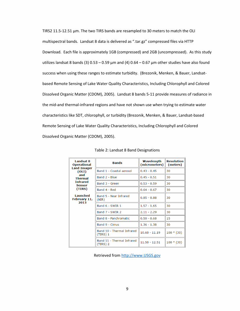
One Landsat 8 scene from the USGS Global Visualization Viewer for August 24th, 2014

was downloaded. The downloaded image is located on path 21 row 32 (see Figure 4 below).

20

Figure 4: Landsat 8 Study Image

Natural Color composite downloaded scene of Path 21 Row 32 from Glovis.USGS.Gov displayed using bands 4,3,2 with overlay of Brookville Reservoir shapefile.

This study utilized calibrated Landsat 8 data with ground-based SDT measurements for

Brookville Lake. The model developed for Brookville Lake was used to estimate SDT

distributions in Eagle Creek and Geist Reservoirs. As Olmanson et al. (2001) mention, SDT depth

should be reported as satellite-estimated SDT values rather than the general term of SDT. The

reason for this is that there are other factors besides algal turbidity that play a part in lake

clarity. A factor that influences the strength of the relationship between field-collected data and

satellite data is the number of pixels included in the area of interest (AOI) (Kloiber, Brezonik,

Olmanson, & Bauer, 2002).

In-situ data collection took place contemporaneously with satellite image acquisition; as

a result, only a small cluster of pixels containing ground data will give the best correlations as

21

determined by data analysis trials. It was determined that when the 30 samples locations or

AOIs had a range of 7 pixels the R2 value equaled 0.580246. When those same 30 AOIs had a

range of 475 pixels the R2 value equaled 0.456423, thus increasing the AOI yielded marginal

benefits.

It is noted that the average brightness data from at least nine pixels in the deep open

area of the lake should be used to predict lake clarity. Kloiber et al. (2002) also writes, increasing

from nine pixels in the AOI did not increase the value and, as long as in-situ data collection were

contemporaneous with the satellite image, a small group of AOIs would provide the best

correlations between satellite and in-situ measurements. This, too, was the case for the

Brookville area study. Increasing the pixel size reduced the accuracy of the model, as shown in

Table 4.

Table 4: Pixel Size vs Accuracy

# of AOI Pixel Range R2 Significance F

30 475 0.456423 0.000266703

30 7 0.580246 8.13644E-06

Utilizing Satellite Imagery to Estimate SDT

Water Only Image

To reduce image size, three water-only images of Brookville, Eagle Creek, and Geist

reservoirs were created from the image downloaded from Glovis.USGS.Gov. The benefit of

creating a water-only image is to conserve file space by removing unnecessary data and to

create an unsupervised classification lake map to act as a guide for selection of the AOIs. The

unsupervised classification images identify classes of pixels that are affected by varying algae

concentrations. Ten different classes were used in the unsupervised classification step, and the

22

classes were color-coded by variations in water quality. Classes that highlighted vegetation,

shoreline, and bottom effects were avoided when choosing sample (AOI) locations on Geist and

Eagle Creek Reservoirs. See unsupervised classification Geist map below.

Figure 5: Unsupervised Classification map of Geist reservoir used as a guide to differentiate vegetation and other classes when selecting AOIs.

Area of Interest (AOI) Creation (Brookville Lake)

One shapefile of 30 sample locations was created corresponding to the collected SDT

measurements at Brookville Lake. This shapefile was then opened on top of the Landsat

satellite scene in Erdas IMAGINE. AOIs were digitized around the SDT measurements for the

Brookville Lake water-only scene. The smallest AOI was 10 pixels and the largest AOI was 17.

Once all the AOIs were drawn around the sample site locations within the satellite scene, each

AOI was added to the signature file. The location ID, pixel count, mean band brightness value,

measured SDT, and lnSDT for each band within the AOI was computed. These results were then

23

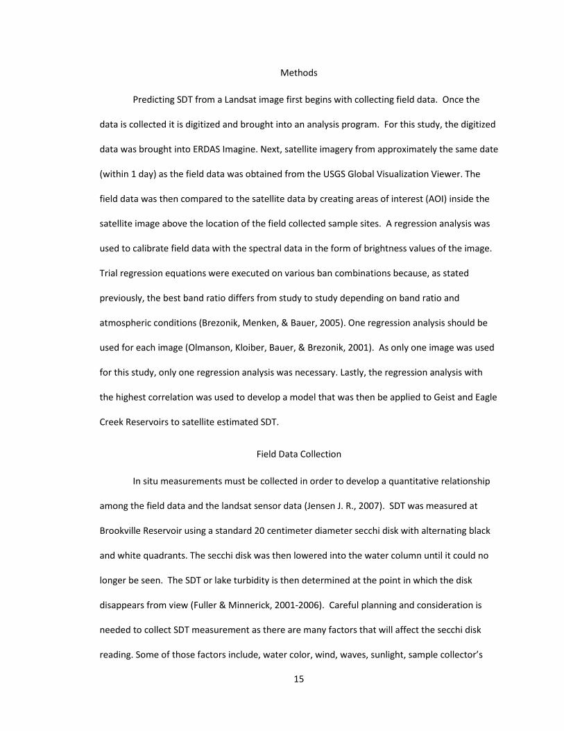
exported into a .dat file format for further calculation. Results for the measurement values

within the corresponding AOIs can be seen in TABLE 5 on next page.

Table 5: Brookville AOIs

SigName PixelCount Mean(Green Band)

Mean(Red Band)

Red Band:Green Band meanSDT(m) ln(sdt)m

Location 1 17 7058.17 6188.82 0.87 0.76 -0.26

Location 2 10 6995.90 6122.50 0.87 0.77 -0.25

Location 3 10 7022.20 6130.60 0.87 0.88 -0.11

Location 4 17 6955.17 6108.05 0.87 0.96 -0.03

Location 5 15 7109.66 6201.26 0.87 0.86 -0.14

Location 6 10 6905.70 6064.00 0.87 1.05 0.05

Location 7 10 6890.50 6070.80 0.88 0.91 -0.08

Location 8 12 6918.66 6071.58 0.87 1.04 0.04

Location 9 10 6911.30 6059.80 0.87 1.00 0.03

Location 10 10 6901.60 6073.90 0.88 0.93 -0.06

Location 11 10 6876.22 6048.11 0.88 0.96 -0.03

Location 12 10 6914.50 6051.70 0.87 1.04 0.04

Location 13 17 6928.47 6068.41 0.87 1.09 0.08

Location 14 14 6934.42 6068.00 0.87 1.06 0.06

Location 15 10 6945.10 6078.80 0.87 1.13 0.12

Location 16 13 7056.30 6139.92 0.87 1.15 0.14

Location 17 10 6992.30 6121.80 0.87 1.06 0.06

Location 18 16 6909.31 6056.87 0.87 1.06 0.06

Location 19 16 6916.93 6063.62 0.87 1.05 0.05

Location 20 17 6912.05 6052.00 0.87 1.08 0.08

Location 21 14 6901.28 6052.28 0.87 1.04 0.04

Location 22 12 6845.08 6029.00 0.88 0.97 -0.02

Location 23 12 6828.33 6012.91 0.88 0.99 -0.05

Location 24 14 6816.07 6015.42 0.88 1.35 0.30

Location 25 15 6823.20 6016.20 0.88 1.25 0.22

Location 26 16 6824.00 6015.18 0.88 1.21 0.19

Location 27 15 6796.06 5998.53 0.88 1.28 0.25

Location 28 14 6773.57 5993.50 0.88 1.26 0.23

Location 29 10 6799.70 5996.80 0.88 1.32 0.28

Location 30 10 6794.00 5992.00 0.88 1.34 0.29

24

Geist and Eagle Creek Reservoirs AOIs

After opening the water-only images of Geist and Eagle Creek (and using an

unsupervised classification map as a guide), AOIs were selected for each of these reservoirs. For

best results, these AOIs should be chosen from areas within the lakes that best represent it

while avoiding areas affected by bottom, shoreline or vegetation effects (Olmanson, Kloiber,

Bauer, & Brezonik, 2001). The location ID, pixel count, and mean band brightness value for each

band within the AOI was computed. These results were then exported into a .dat file format for

further calculation. As no in-situ measurements were recorded at these two reservoirs, the

mean brightness value data was used in the final model to generate predicted SDT. An example

of the AOI selection can be seen in FIGURE 6.

Figure 6: AOI Selection of Eagle Creek

25

Results

Regression Equations and Tests of Significance

With brightness values obtained for 30 AOIs in Brookville reservoir, trial regression

analysis were computed for Brookville Reservoir based on the equation developed by Kloiber et

al. (2002):

ln(SDT) = a(TM1/TM3) + bTM1+ c

As the Kloiber et al. equation addressed satellite imagery from Landsat 7, further

regression analysis was needed to verify which Landsat 8 bands had the best correlation values.

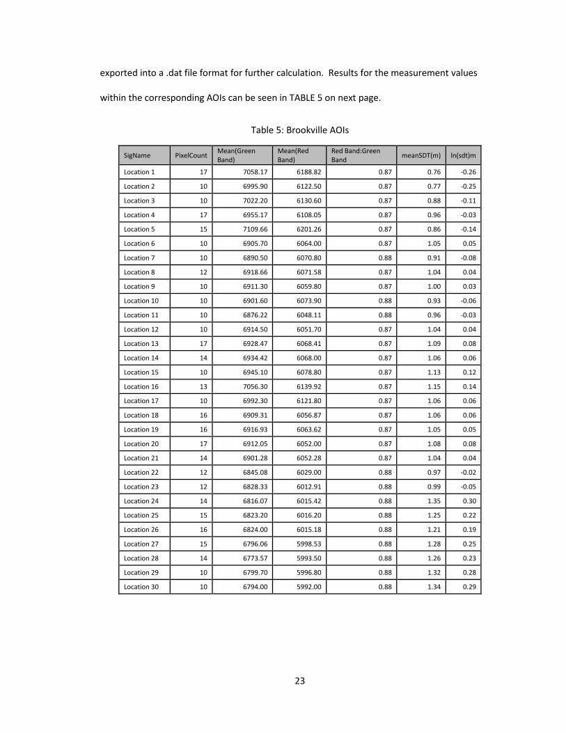
Analysis focused on Landsat 8 combinations of band 2, band 3, and band 4. As is noted in TABLE

6, band 4/band 3 + band 4 had the strongest relationship with SDT (R2=.58, Significance F=

8.13644E-06).

Table 6: Band Combinations Trials

Blue Band : Red Band R2 0.5590 Significance F 1.58E-05

Green Band: Red Band R2 0.5783 Significance F 8.65E-06

Red Band: Green Band R2 0.5802 Significance F 8.14E-06

Red Band: Blue Band R2 0.5589 Significance F 1.59E-05

Blue Band: Green Band R2 0.4901 Significance F 0.0001

Green Band: Blue Band R2 0.4881 Significance F 0.0001

26

Therefore, the final model to convert satellite image brightness values to predicted ln(SDT) is:

ln(SDT)=a(Band4:Band3)+b(Band4)+c. The corresponding SDT predicted values can then be

calculated by the following equation: e^(ln(SDT)) = SDT.

The data was transferred into Excel’s Analysis ToolPak for multiple regression

calculations. The regression equations and data are listed below in TABLE 7. A further

breakdown of the final model is listed in TABLE 8.

The resultant r2 value of this study (r2=0.5802) was less than the r2 value obtained in the

Kloiber et al. study of r2=0.67. Some differences between the numbers was expected as the

band wavelengths for the two studies were different. It was hoped that the Landsat 8 r2 values

would be higher as the Landsat 8 band wavelengths are narrower than the bands used in the

study be Kloiber et al. A table with the final predicted SDT values for Geist and Eagle Creek

reservoirs is shown in Table 9.

Table 7: Regression Data

Regression Statistics

R Square 0.5802

Significance F 8.1364E-06

Coefficients

Intercept 24.9021

X Variable 1 -10.4643

X Variable 2 -0.0026

27

Table 8: Final Model

"Y = (X Variable 1)(MeanRedBand:MeanGreenBand) + (X Variable 2)(MeanRedBand) + Intercept "

"ln(SDT) = -10.4643(MeanRedBand:MeanGreenBand) - 0.0026(MeanRedBand) + 24.9021"

"SDT = EXP(ln(SDT))"

Table 9: Predicted vs. Actual SDT

R² = 0.5802

0.600.700.800.901.001.101.201.301.401.50

0.60 0.70 0.80 0.90 1.00 1.10 1.20 1.30 1.40 1.50

Pred

icte

d Se

cchi

-Dis

k Tr

ansp

aren

cy, i

n M

eter

s

Actual Secchi-Disk Transparnecy, in Meters

Predicted and Actual SDT for Landsat 8 path 21, row 32

28

Table 10: Predicted SDT values for Eagle Creek and Geist Reservoirs.

Geist Eagle Creek Location SDT (m)

Location SDT (m)

1 0.2283

1 0.4619 2 0.2329

2 0.4318

3 0.6136

3 0.4520 4 0.4852

4 0.3450

5 0.6595

5 0.3900 6 0.6283

6 0.2303

7 0.6573

7 0.2862 8 0.4882

8 0.3929

9 0.3268

9 0.3079 10 0.5085

10 0.4572

11 0.5027

11 0.3521 12 0.5434

12 0.3896

13 0.5146

13 0.4561 14 0.5985

14 0.4481

15 0.5623

15 0.4479 16 0.5598

16 0.4315

17 0.5244

17 0.4305 18 0.5442

18 0.3660

19 0.5499

19 0.4117 20 0.5787

20 0.4399

21 0.6352

21 0.4313 22 0.6239

22 0.4405

23 0.6181

23 0.5603 24 0.6025

24 0.5466

25 0.6462

25 0.5536 26 0.5883

26 0.5405

27 0.6430

27 0.5772 28 0.6575

28 0.5762

29 0.6889

29 0.5443 30 0.6840

30 0.5493

31 0.6821

31 0.5710 32 0.7099

32 0.5405

33 0.6888

33 0.5680 34 0.6659

34 0.5750

35 0.6818

35 0.5632 36 0.6348

36 0.5683

37 0.6653

37 0.6107 38 0.6138

38 0.5829

39 0.6605

39 0.5905 40 0.6534

40 0.6117

41 0.6520

41 0.6329 42 0.6078

42 0.5952

43 0.6787

43 0.5909 44 0.7116

44 0.5818

45 0.7032 45 0.6176

29

Figure 7: Predicted SDT Map for Eagle Creek Reservoir

30

Figure 8: Predicted SDT Map for Geist Reservoir

31

Conclusions

This study utilized a Landsat 8 satellite scene located in central Indiana and 30 SDT

measurements to find the best method of predicting SDT for lakes in the same image. SDT data

was collected at Brookville Reservoir on August 24, 2014. A regression model was developed to

predict SDT levels at the unsampled reservoirs, Geist and Eagle Creek. The corresponding

satellite image was downloaded to obtain the necessary brightness values. Regression analysis

was performed using several different bands within Landsat 8. After comparing the calculated

R2 and Significant F values for each of the different bands, a reasonable model was developed

that can be used to predict SDT levels from the corresponding Landsat 8 images. SDT and

turbidity have been shown to be highly correlated and act as a measure of algal abundance in

Geist, Eagle Creek, and Brookville reservoirs. Red Band/Green Band + Red Band yielded the

highest R2 and Significant F values and were used for further analysis on the un-sampled Geist

and Eagle Creek Reservoirs to determine SDT depths. The results show that SDT can be

estimated from Landsat 8 data as long as near contemporaneous in situ measurements are

collected. These results confirm previous studies like Olmansen et al. (2002), Brezonik et al.

(2005), Bonansea et al. (2015). These remote sensing techniques offer a low-cost method of

water quality determination. Validation is necessary for the predictive model used to estimate

SDT depth in the unsampled reservoirs. The secchi disk depth given for Geist and Eagle Creek

are quantitative estimates and must be verified in order for this model to be useful.

Predictive models make assumptions related to distribution. In order to verify the

predicted depths, residuals may be studied to further evaluate the validity of the model or in

situ samples of the unsampled reservoirs will aid in the verification of predicted SDT depths.

32

Suggestions for future tests regarding water quality monitoring using secchi disk consist

of taking samples before and after the image acquisition. This may be beneficial in establishing

a more representative outline of SDT levels and help eliminate any doubt of secchi disk user

calculation error that may have occurred due to the angle of the sun or varying conditions of the

waterbody. With a more comprehensive dataset, a model could potentially be developed with a

higher degree of correlation.

33

References

Bonansea, M., Rodriguez, M., Pinotti, L., & Ferrero, S. (2014). Using multi-temporal Landsat

imagery and linear mixed models for assessing water quality parameters in Rio Tercero

reservoir. Remote Sensing of Environment, 28-41.

Brezonik, P., Menken, K. D., & Bauer, M. (2005). Landsat-based Remote Sensing of Lake Water

Quality Characteristics, Including Chlorophyll and Colored Dissolved Organic Matter

(CDOM). Lake and Reservoir Management, 373-382.

Center for Earth and Environmental Science. (2015, March 3). What causes algal blooms?

Retrieved from www.cees.iupui.edu/research:

http://www.cees.iupui.edu/research/algal-toxicology/bloomfactors

Eagle Creek Advisory Committee. (1997). Eagle Creek Park Master Plan.

Fuller, L. M., & Minnerick, R. J. (2001-2006). Predicting Water Quality by Relating Secchi-Disk

Transparency and Chlorophyll-a Measurements to Landsat Satellite Imagery for

Michigan Inland Lakes. United States Geological Survey.

Indiana Clean Lakes Program. (2011). Volunteer Lake Monitoring Manual. Bloomington: School

of Public and Environmental Affairs-Indiana University.

Indiana Department of Environmental Management . (2015, March 5). Addressing Concerns

About Blue-Green Algae . Retrieved from http://www.in.gov/idem/algae/2310.htm#

Indiana Department of Natural Resources. (2011). Brookville Reservoir Whitewater Memorial

State Park Interpretive Master Plan. Indiana Department of Natural Resources.

Jensen, J. R. (1983). Biophysical Remote Sensing. Annals of the Association of American

Geographers, 111-132.

Jensen, J. R. (2007). Remote Sensing of the Environment. Upper Saddle River: Pearson Prentice

Hall.

34

Kloiber, S. M., Brezonik, P. L., Olmanson, L. G., & Bauer, M. E. (2002). A procedure for regional

lake water clarity assessment using Landsat multispectral data. Remote Sensing of

Environment, 38-47.

Knight, J. F., & Voth, M. L. (2012). Application of MODIS Imagery for Intra-Annual Water Clarity

Assessment of Minnesota Lakes. Remote Sensing, 2181-2198.

Kudela, R. M., Palacios, S. L., Austerberry, D. C., Accorsi, E. K., Fuild, L. S., & Torres-Peres, J.

(2015). Application of hyperspectral remote sensing to cyanobacterial blooms in inland

waters. Remote Sensing of Environment.

Landsat Science. (2014, June 6). Retrieved June 9, 2014, from NASA.GOV:

http://landsat.gsfc.nasa.gov/?page_id=7195

McCullough, I. M., Loftin, C. S., & Sader, S. A. (2012). Combining lake and watershed

characteristics with Landsat TM data for remote estimation of regional lake clarity.

Remote Sensing of Environment, 109-115.

Olmanson, L. G., Kloiber, S. M., Bauer, M. E., & Brezonik, P. L. (2001). Image processing protocol

for regional assessments of lake water quality. St. Paul: Water Reources Center and

Remote Sensing Laborator University of Minnesota.

Powell, R., Brooks, C., French, N., & Shuchman, R. (2009). Remote Sensing of Lake Clarity. Ann

Arbor: Michigan Tech Research Institute.

Roy, D. P., Wulder, M. A., Loveland, T. R., Woodcock, C. E., Allen, R. G., Anderson, M. C., . . . Zhu,

Z. (2014). Landsat-8: Science and product vvision for terrestrial global change research.

Remote Sensing of Environment, 154-172.

Schlacher, T. A., Lloyd, S., & Wiegand, A. (2010). Use of local ecological knowledge in the

management of algal blooms. Environmental Conservation , 210-221.

35

Srriwongsitanon, N., Surakit, K., & Thianpopirug, S. (2011). Influence of atmospheric correction

and number of sampling points on the accuracy of water clarity assessment using

remote sensing application. Journal of Hydrology, 203-220.

Tebbs, E. J., Remediios, J. J., & Harper, D. M. (2013). Remote sensing of chlorophyll-a as a

measure of cyanobacterial biomass in Lake Borgoria, a hypertrophic, saline-alkaline,

flamingo lake using Landsat ETM+. Remote Sensing of Environment, 92-106.

U.S. Geological Survery. (2015, March 3). Bands Designations for Landsat satellites . Retrieved

from Landsat.USGS.Gov:

http://landsat.usgs.gov/band_designations_landsat_satellites.php

United States Environmental Protection Agency. (2013, February 15). Impacts of Climate

Change. Retrieved from

http://www2.epa.gov/sites/production/files/documents/climatehabs.pdf

V3 Companies. (2011). Geist Reservoir/Upper Fall Creek Watershed Management Plan.

Wynne, T. (2013, March 23). NOAA Ocean Science Blog. Retrieved from

https://noaaoceanscience.wordpress.com/2013/05/23/nccos-continues-issuing-weekly-

lake-erie-harmful-algal-bloom-forecasts/

CURRICULUM VITAE

Miranda J. Hancock

Education

Indiana University – Purdue University Indianapolis M.S., Geographic Information Science August 2015 Indiana University – Purdue University Indianapolis B.A. Geography May 2010 Professional Experience Indiana Department of Environmental Management -- Indianapolis, IN -- August 2014-Present Senior Environmental Manager

• Business process research and analysis • Project management documentation outlining work structure, project schedule • Conduct User Assistance Testing with Management, Permit Writers, and

Administrative staff (SharePoint, Syncplicity, Modelers Utility) • Develop user guides for Permit Writers, Administrative staff, and Management • Conduct user trainings and continue post-implementation support for

SharePoint and Modelers Utility (ArcMap) • Stream Modeling/Wasteload Allocation analyses • Provide cross functional networking with permittees, consultants, IDEM

associates, and EPA to assure state regulatory compliance • Develop statewide Industrial NPDES permits • Conduct site visits with facilities, consultants, stakeholders • Create and maintain geodatabases

Indiana Department of Environmental Management -- Indianapolis, IN -- August 2011-August 2014 Environmental Manager

• Developed statewide Industrial NPDES permits • Provide cross functional networking with permittees, consultants, IDEM

associates, and EPA to assure state regulatory compliance • Developed CSO (combined sewer overflow) ArcMap utility • Developed a paperless permitting system for entire permit branch utilizing

SharePoint and ArcMap

• Draft Preliminary Effluent Limitations and possess wasteload allocation knowledge

The Polis Center at IUPUI – Indianapolis, IN— June 2010 – August 2011 GIS Analyst

• Design, development, testing, implementation, and analysis of GIS applications and models

• Developed multi-hazard mitigation plans using ArcGIS for municipalities in Indiana

• Project management documentation outlining work structure, project schedule, timeline

• Seamline editing using advanced orthorectification software • Orthoimagery QC • Create and Maintain geodatabases • Develop training curriculum for HAZUS-MH and ESRI users • Map Modernization • Graphic editing of feature datasets using latest versions of ESRI software

Indiana Department of Natural Resources – Indianapolis, IN— September 2008 – June 2010 Engineering Assistant

• Collected, analyzed, and interpreted hydrologic information collect in field studies and assisted in displaying the information collected through ArcGIS

• Installed, maintained, serviced, and troubleshot sensing, recording, and communication equipment and instrumentation

• Review well logs containing statistical and technically hydrologic data collected in field

Indiana Department of Environmental Management – Indianapolis, IN -- Summer 2008 Ground Water Section, Intern

• Collected, analyzed, and interpreted hydrologic information collect in field studies and assisted in displaying the information collected through ArcGis

• Performed field water-quality measurements such as water temperature, specific conductance, pH, dissolved oxygen, and alkalinity

• Collected, processed, prepared, and delivered samples to lab for analyses • Assembled, evaluated and prepared field and laboratory data for tabulation,

analysis, and publication • Installed, maintained, serviced, and troubleshot sensing, recording, and

communication equipment and instrumentation • Calibrated meters and analytical equipment using appropriate techniques and

protocols


Recommended