116

An analytical methodology for prediction of the platoon arrival profilesand queue length along signalized arterials is proposed. Traffic betweensuccessive traffic signals is modeled as a two-step Markov decision process(MDP). Traffic dynamics are modeled with the use of the kinematic wavetheory. The MDP formulation allows prediction of the arrival profiles sev-eral signals downstream from a known starting flow. This modelingapproach can be used to estimate queue lengths and predict travel times,even in cases in which data from loop detectors are unknown, inaccurate,or aggregated. The proposed model was applied to two real-world testsites. The queues estimated with the model are in close agreement with theresults from microscopic simulation.

A significant proportion of travel takes place on urban arterials con-trolled by traffic signals. Monitoring of system performance on arteri-als and evaluation of alternative traffic management strategies requireanalysis tools for accurate estimation of the queue lengths at the inter-section approaches, the travel times on the arterial links, and othermeasures. A number of techniques have been developed to estimatearterial performance measures from surveillance data. Most of the pro-posed models, however, are quite site specific and cannot be readilyapplied to other locations.

There is a need for models that can be used to estimate travel timeson arterial streets on the basis of conventional loop detector data (flow,speed, and occupancy). Such models should be based on realisticmodeling of traffic dynamics to predict accurately the interaction ofvehicles as they travel along the arterials and the queues formed at thesignalized intersections. At the same time, such models should berobust and should be able to provide performance measures even withfaulty or limited detector data.

The objective of the study described here is to develop an analyticalmodel that can be used to estimate platoon dispersion on arterial linksand queues at traffic signals. This is an important part of on ongoingstudy to develop a system for the online estimation of arterial traveltimes from surveillance data.

The paper first briefly reviews existing platoon dispersion mod-els. Next, the model formulation for estimation of the platoon dis-persion and queue lengths at signalized intersections is described.The last section presents the application of the proposed model ontwo test sites and outlines ongoing and future model enhancements.

BACKGROUND

The traffic departing a traffic signal initially moves as a tight pla-toon with short vehicle headways. This platoon tends to disperse thefarther downstream that it travels because of differences in vehiclespeeds, vehicle interactions (lane changing and merging), and otherinterferences (parking, pedestrians, and other frictional effects) (1).Prediction of platoon size and dispersion is important for determi-nation of the traffic arrivals at downstream intersections to assessthe need for signal coordination and to optimize the signal timingplans in coordinated signal systems.

Pacey modeled platoon dispersion by assuming that the speed ofany single vehicle traveling on an arterial link is constant and unre-stricted overtaking (2). He derived the travel time distribution, g(τ),along the arterial segment by also assuming that the vehicle speedsare normally distributed:

where

D = distance from the upstream signal to a downstreamlocation where the vehicle arrivals are observed;

τ = individual vehicle travel time along distance D; andu– and σ = mean and standard deviation of vehicle speeds, respec-

tively.

The number of vehicles passing the downstream observation point(Location 2) in the time interval (t, t + dt) [q2(t2)dt2] is

where q1(t1)dt1 is the number of vehicles passing the upstream signal(Location 1) in the interval (t, t + dt), and g(t2 − t1) is the probabilitydensity function of travel time (t2 − t1) according to Equation 1.

Robertson’s formula (3), implemented in the TRANSYT simulationand optimization model, is the most well-known model of platoondispersion. It is similar to the discrete version of Pacey’s model, butit has been derived by assuming a geometric distribution of vehicletravel times:

q i tt

q it

q i t2 1 2

1

11

1

11 3+( ) =

+( ) + −

+⎛⎝

⎞⎠ + −( )

α α( )

q t dt q t g t t dt dtl

2 2 2 1 1 2 1 1 21

2( ) = ( ) −( )∫ ( )

gD

Du

ττ σ π

τσ

( ) = −−⎛

⎝⎞⎠

⎡

⎣⎢⎢

⎤

⎦⎥⎥2

2

22 21exp ( )

Prediction of Arrival Profiles and QueueLengths Along Signalized Arterials byUsing a Markov Decision Process

Nikolaos Geroliminis and Alexander Skabardonis

Institute of Transportation Studies, University of California, Berkeley, 109 McLaughlinHall, Berkeley, CA 94720-1720.

Transportation Research Record: Journal of the Transportation Research Board, No. 1934, Transportation Research Board of the National Academies, Washington,D.C., 2005, pp. 116–124.

Geroliminis and Skabardonis 117

where

L = signal spacing,uf = free-flow speed, andf = platoon dispersion function

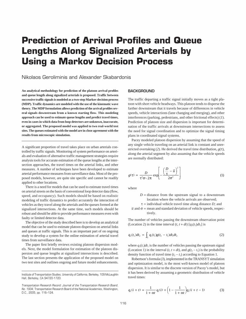
Thus, by alternating the platoon dispersion process with the sig-nal filter one, the arrival profiles at several intersections downstreamcan be predicted from a known starting flow. A schematic repre-sentation of the algorithm is shown in Figure 1. This formulation canbe used to predict travel times and estimate queue lengths, even incases in which traffic flow data from loop detectors are unknown,inaccurate, or aggregated.

In the case of incomplete information regarding the signal settings(e.g., actuated signals with variable green times), the formulation hasstochastic characteristics and is an MDP. This process has the Markovproperty, as given the present arrivals An from signal n, the distribu-tion of An +1 is determined. This can be restated as the probability thatAn +1, which is conditional on the whole past history of the sequence(Am = im)n

m = 1 (where m is an index and m = 1 to n indicates the arrivalsfor all signals upstream of n + 1), reduces to a probability of An +1 con-ditional on the latest value alone, An. Given that the signal settingsare fixed, MDP is equivalent to a one-step recursion, as shown above.

where P is probability, and in is the state (arrival’s profile) at signal n.

Estimation of Platoon Dispersion

Platoon dispersion was modeled by using the kinematic wave theoryproposed by Lighthill and Whitham (6 ) and Richards (7 ) (the LWRtheory). The main postulate of the LWR theory is that a functional rela-tionship exists between the traffic flow (q) and the traffic density (k)and that this relationship could be used to describe the speed at whicha change in traffic flow propagates either downstream or upstreamfrom an origin point. Shock waves are generated by the traffic sig-nal, which causes congested conditions to develop near the stop lineduring the red time and capacity conditions to occur when the queueis discharging at the saturation flow rate. The first vehicle departs fromthe stop line at the free-flow speed, but because of interfaces betweendifferent points of the q–k diagram, the following vehicles departfrom the stop line at slower speeds. The level of dispersion in speedsand, as a result, in the platoon depends on the curvature of theincreasing part of the q–k diagram.

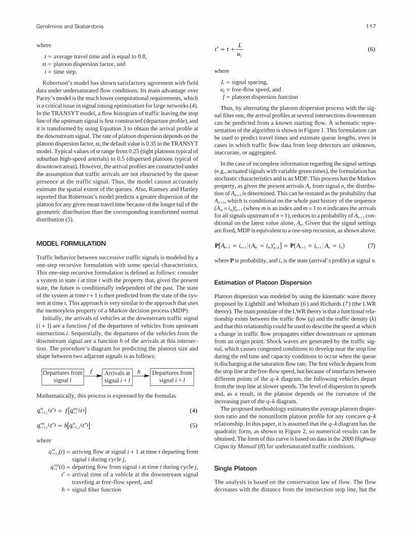
The proposed methodology estimates the average platoon disper-sion ratio and the nonuniform platoon profile for any concave q–krelationship. In this paper, it is assumed that the q–k diagram has thequadratic form, as shown in Figure 2, so numerical results can beobtained. The form of this curve is based on data in the 2000 HighwayCapacity Manual (8) for undersaturated traffic conditions.

Single Platoon

The analysis is based on the conservation law of flow. The flowdecreases with the distance from the intersection stop line, but the

P PA i A i A i A in n m m mn

n n n n+ + = + += =( )[ ] = = =( )1 1 1 1 1 7� � ( )

′ = +t tL

uf

( )6where

t = average travel time and is equal to 0.8,α = platoon dispersion factor, andi = time step.

Robertson’s model has shown satisfactory agreement with fielddata under undersaturated flow conditions. Its main advantage overPacey’s model is the much lower computational requirements, whichis a critical issue in signal timing optimization for large networks (4).In the TRANSYT model, a flow histogram of traffic leaving the stopline of the upstream signal is first constructed (departure profile), andit is transformed by using Equation 3 to obtain the arrival profile atthe downstream signal. The rate of platoon dispersion depends on theplatoon dispersion factor, α; the default value is 0.35 in the TRANSYTmodel. Typical values of α range from 0.25 (tight platoons typical ofsuburban high-speed arterials) to 0.5 (dispersed platoons typical ofdowntown areas). However, the arrival profiles are constructed underthe assumption that traffic arrivals are not obstructed by the queuepresence at the traffic signal. Thus, the model cannot accuratelyestimate the spatial extent of the queues. Also, Rumsey and Hartleyreported that Robertson’s model predicts a greater dispersion of theplatoon for any given mean travel time because of the longer tail of thegeometric distribution than the corresponding transformed normaldistribution (5).

MODEL FORMULATION

Traffic behavior between successive traffic signals is modeled by aone-step recursive formulation with some special characteristics.This one-step recursive formulation is defined as follows: considera system in state i at time t with the property that, given the presentstate, the future is conditionally independent of the past. The stateof the system at time t + 1 is then predicted from the state of the sys-tem at time t. This approach is very similar to the approach that usesthe memoryless property of a Markov decision process (MDP).

Initially, the arrivals of vehicles at the downstream traffic signal(i + 1) are a function f of the departures of vehicles from upstreamintersection i. Sequentially, the departures of the vehicles from thedownstream signal are a function h of the arrivals at this intersec-tion. The procedure’s diagram for predicting the platoon size andshape between two adjacent signals is as follows:

Mathematically, this process is expressed by the formulas

where

q ini+1,j(t) = arriving flow at signal i + 1 at time t departing from

signal i during cycle j,q i,j

out(t) = departing flow from signal i at time t during cycle j,t′ = arrival time of a vehicle at the downstream signal

traveling at free-flow speed, andh = signal filter function

q t h q ti j i j+ +′( ) = ′( )[ ]1 1 5, , ( )out in

q t f q ti j i j+ ′( ) = ( )[ ]1 4, , ( )in out

Departures fromsignal i

Arrivals atsignal i + l

Departures fromsignal i + l

f h

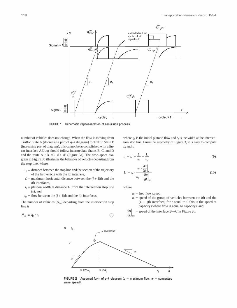
number of vehicles does not change. When the flow is moving fromTraffic State A (decreasing part of q–k diagram) to Traffic State E(increasing part of diagram), this cannot be accomplished with a lin-ear interface AE but should follow intermediate States B, C, and Dand the route A→B→C→D→E (Figure 3a). The time–space dia-gram in Figure 3b illustrates the behavior of vehicles departing fromthe stop line, where

Li = distance between the stop line and the section of the trajectoryof the last vehicle with the ith interface,

t′i = maximum horizontal distance between the (i + 1)th and theith interfaces,

ti = platoon width at distance Li from the intersection stop line(s), and

qi = flow between the (i + 1)th and the ith interfaces.

The number of vehicles (Ntot) departing from the intersection stopline is

N q ttot = 0 0 8� ( )

118 Transportation Research Record 1934

where q0 is the initial platoon flow and t0 is the width at the intersec-tion stop line. From the geometry of Figure 3, it is easy to computeLi and ti

where

uf = free-flow speed;ui = speed of the group of vehicles between the ith and the

(i + 1)th interface; for i equal to 0 this is the speed atcapacity (where flow is equal to capacity); and

= speed of the interface B→C in Figure 3a.∂∂q

k BC

L tu

qk

uqk

i =

∂∂

− ∂∂

0

0

0

10��

BC

BC

( )

t tL

u

L

ui

i i

f

= + −00

9( )

extended red forcycle j+1 atsignal i+1

Signal i+1

Signal i

cycle j cycle j+1

ufu fu f

t

x

q i, j+1out

q i+1,jout

q i+1,j+1out

q i+1,jin

q i+1,j+1in

q i, jout

FIGURE 1 Schematic representation of recursion process.

w

0.25kj kj0.125kj

q

c

k

quadratic

uf

FIGURE 2 Assumed form of q–k diagram (c � maximum flow; w � congestedwave speed).

of the red phase. This methodology is expressed as a first-order approx-imation because the pattern of the dispersion is not estimated; just theaverage value of the arrival flow is estimated. To estimate the shapeof the platoon arrivals (flow in a time–space region), the followingshould be added to Equations 11 to 14:

where n is the number of steps in the finite differences procedure.The time τij in Equation 15 shows the amount of time in the pla-

toon pattern at distance Li downstream of the signal that the flow isequal to qj. Therefore, Figure 3b shows that

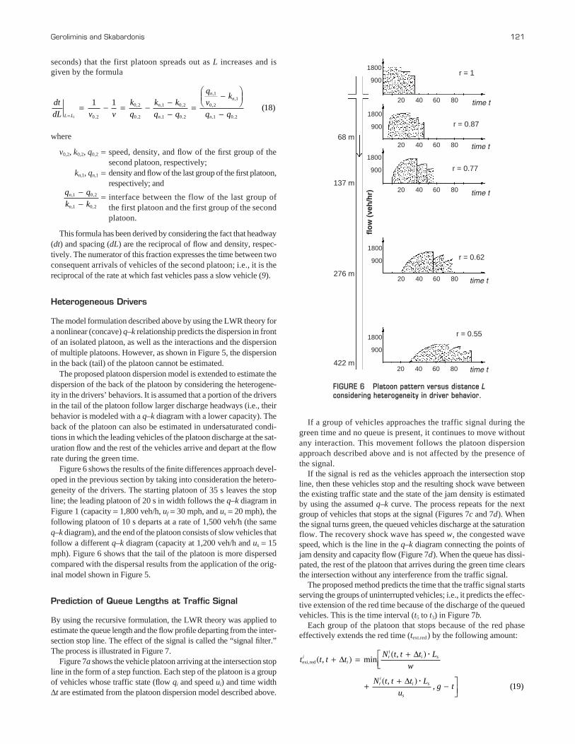
Figure 5 shows the results of the finite differences approach for astarting platoon of 20 s in width departing at capacity [1,800 vehiclesper hour (veh/h)] from the stop line and under the assumption of a qua-dratic form for the increasing part of the q–k diagram with a free-flow

τ

τ

ij

j i

j n

j i i

ij i

q L t

t

=

=

∑ ( ) =

= ′

,

( )

and

17

τin n ii

n

i

f

q LL

q

L

u, ( )( ) =

′−

−1

16

τij j ii

j

i

j

q LL

q

L

qj j i, : ( )( ) =

′−

′∀ ≥

−1

15

Geroliminis and Skabardonis 119

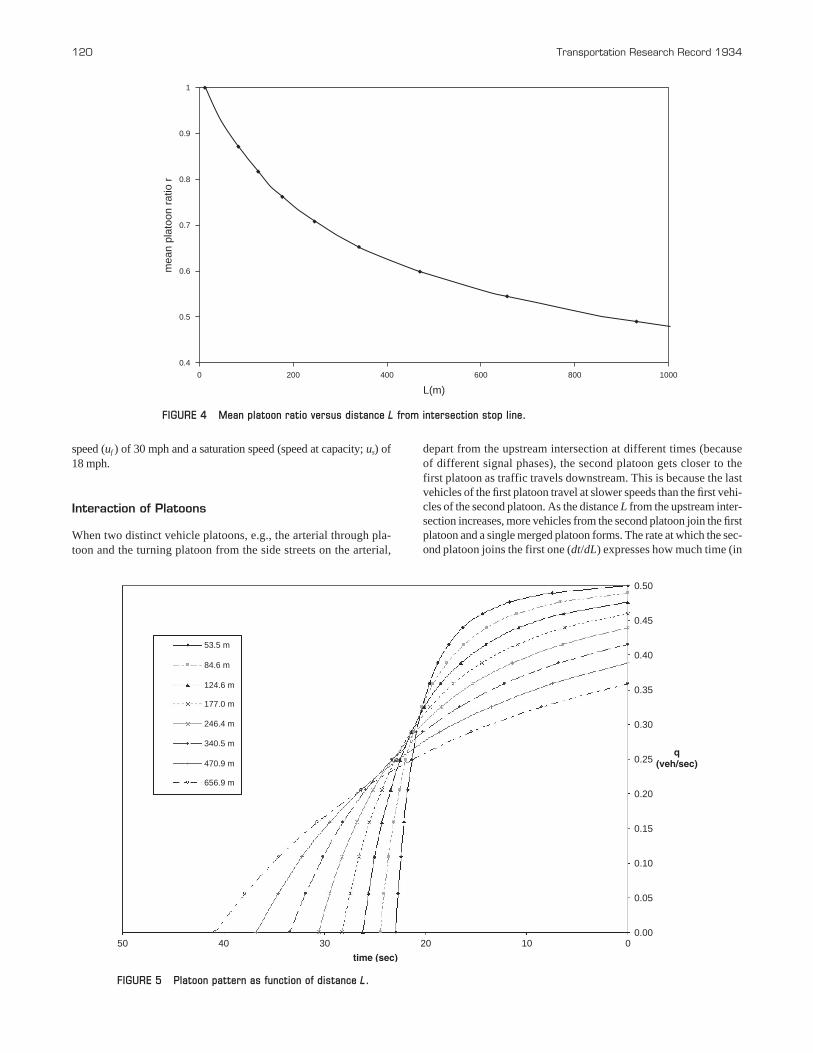
For simplicity, the speed of the ith interface is indicated as q ′i. Theplatoon dispersion ratio (ri) at distance Li downstream from the signalis equal to

A numerical approach with finite differences was developed to esti-mate ti and ri at a distance Li from the intersection stop line (Figure 4).The finite differences equations are

The approach described above allows the average flow rate to beestimated as a function of distance L from the beginning of the pla-toon. It should be mentioned that distance L is not the distance fromthe first upstream signal. It shows the average arrival flow of vehiclesat distance Li downstream of a signal where vehicles stopped because

′ = ′ − ′′ ′

−

−

t Lq q

q qi i

i i

i i

��

1

1

14( )

L L tq u

u qi i i

i i

i i

− = ′ ′− ′− −

− −

− −1 1

1 1

1 1

13��

( )

t tL L

u

L L

ui i

i i

i

i i

f

= + − − −−

−

−

−1

1

1

1 12( )

rq

q

Nt

Nt

t

ti

i i

i

= =

⎛⎝⎜

⎞⎠⎟

⎛⎝⎜

⎞⎠⎟

=0

0

0 11

tot

tot

( )

(b)

(a)

x

t

L1

t1

t1τij

t0

uB

uc

uf

trajectories

interfaces

q

k

speeds

interfaces

E

D

CB

A

FIGURE 3 Estimation of platoon dispersion: (a) speed and interfaces in the q–kdiagram and (b) x–t diagram for estimation of platoon dispersion.

120 Transportation Research Record 1934

L(m)

mea

n pl

atoo

n ra

tio r

0

0.4

0.5

0.6

0.7

0.8

0.9

1

200 400 600 800 1000

FIGURE 4 Mean platoon ratio versus distance L from intersection stop line.

time (sec)

q(veh/sec)

010203040500.00

0.05

0.10

0.15

0.20

53.5 m

84.6 m

124.6 m

177.0 m

246.4 m

340.5 m

470.9 m

656.9 m

0.25

0.30

0.35

0.40

0.45

0.50

FIGURE 5 Platoon pattern as function of distance L.

speed (uf ) of 30 mph and a saturation speed (speed at capacity; us) of18 mph.

Interaction of Platoons

When two distinct vehicle platoons, e.g., the arterial through pla-toon and the turning platoon from the side streets on the arterial,

depart from the upstream intersection at different times (becauseof different signal phases), the second platoon gets closer to thefirst platoon as traffic travels downstream. This is because the lastvehicles of the first platoon travel at slower speeds than the first vehi-cles of the second platoon. As the distance L from the upstream inter-section increases, more vehicles from the second platoon join the firstplatoon and a single merged platoon forms. The rate at which the sec-ond platoon joins the first one (dt/dL) expresses how much time (in

seconds) that the first platoon spreads out as L increases and isgiven by the formula

where

v0,2, k0,2, q0,2 = speed, density, and flow of the first group of thesecond platoon, respectively;

kn,1, qn,1 = density and flow of the last group of the first platoon,respectively; and

= interface between the flow of the last group ofthe first platoon and the first group of the secondplatoon.

This formula has been derived by considering the fact that headway(dt) and spacing (dL) are the reciprocal of flow and density, respec-tively. The numerator of this fraction expresses the time between twoconsequent arrivals of vehicles of the second platoon; i.e., it is thereciprocal of the rate at which fast vehicles pass a slow vehicle (9).

Heterogeneous Drivers

The model formulation described above by using the LWR theory fora nonlinear (concave) q–k relationship predicts the dispersion in frontof an isolated platoon, as well as the interactions and the dispersionof multiple platoons. However, as shown in Figure 5, the dispersionin the back (tail) of the platoon cannot be estimated.

The proposed platoon dispersion model is extended to estimate thedispersion of the back of the platoon by considering the heterogene-ity in the drivers’ behaviors. It is assumed that a portion of the driversin the tail of the platoon follow larger discharge headways (i.e., theirbehavior is modeled with a q–k diagram with a lower capacity). Theback of the platoon can also be estimated in undersaturated condi-tions in which the leading vehicles of the platoon discharge at the sat-uration flow and the rest of the vehicles arrive and depart at the flowrate during the green time.

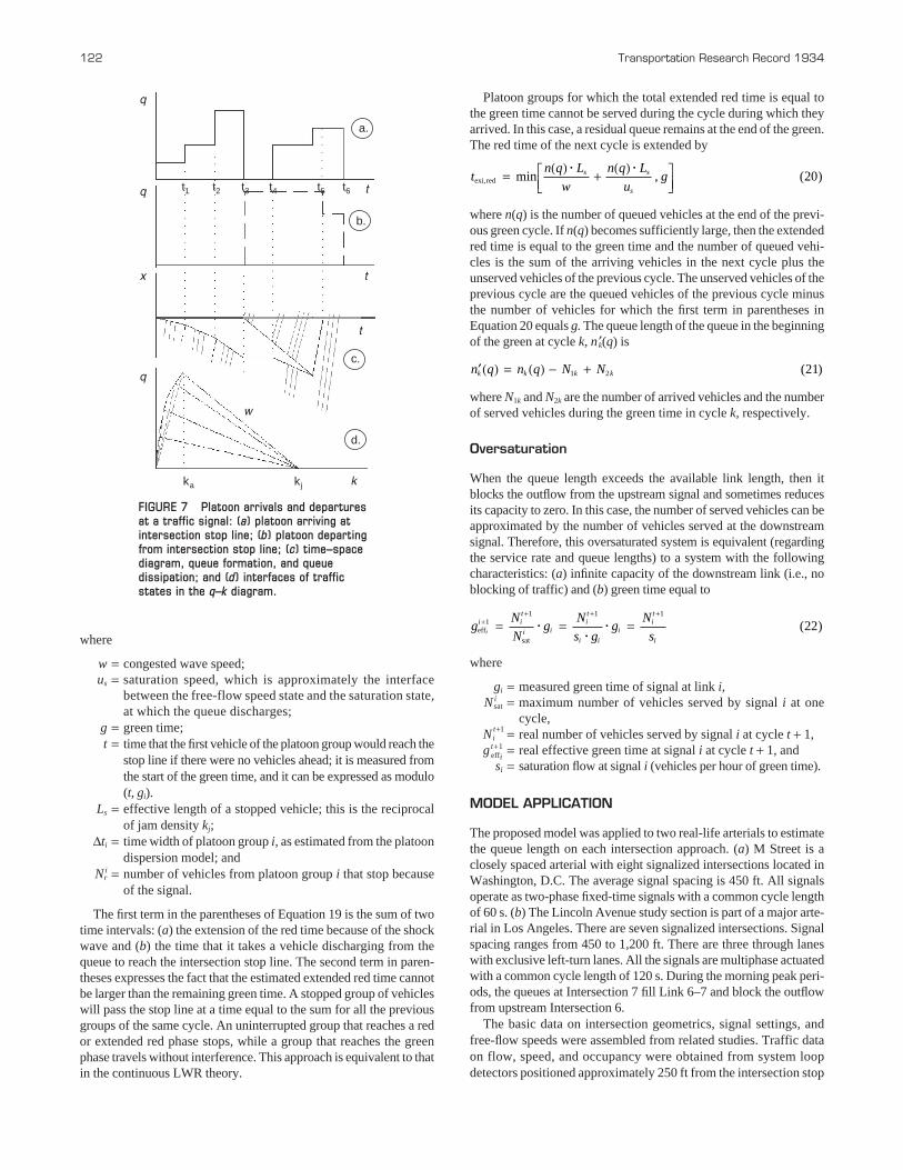
Figure 6 shows the results of the finite differences approach devel-oped in the previous section by taking into consideration the hetero-geneity of the drivers. The starting platoon of 35 s leaves the stopline; the leading platoon of 20 s in width follows the q–k diagram inFigure 1 (capacity = 1,800 veh/h, uf = 30 mph, and us = 20 mph), thefollowing platoon of 10 s departs at a rate of 1,500 veh/h (the sameq–k diagram), and the end of the platoon consists of slow vehicles thatfollow a different q–k diagram (capacity at 1,200 veh/h and us = 15mph). Figure 6 shows that the tail of the platoon is more dispersedcompared with the dispersal results from the application of the orig-inal model shown in Figure 5.

Prediction of Queue Lengths at Traffic Signal

By using the recursive formulation, the LWR theory was applied toestimate the queue length and the flow profile departing from the inter-section stop line. The effect of the signal is called the “signal filter.”The process is illustrated in Figure 7.

Figure 7a shows the vehicle platoon arriving at the intersection stopline in the form of a step function. Each step of the platoon is a groupof vehicles whose traffic state (flow qi and speed ui) and time width Δt are estimated from the platoon dispersion model described above.

q q

k kn

n

, ,

, ,

1 0 2

1 0 2

−−

dt

dL v v

k

q

k k

q q

qv

k

q qL L

n

n

nn

ni== − = − −

−=

−⎛⎝⎜

⎞⎠⎟

−1 1

180 2

0 2

0 2

1 0 2

1 0 2

1

0 21

1 0 2,

,

,

, ,

, ,

,

,,

, ,

( )

Geroliminis and Skabardonis 121

If a group of vehicles approaches the traffic signal during thegreen time and no queue is present, it continues to move withoutany interaction. This movement follows the platoon dispersionapproach described above and is not affected by the presence ofthe signal.

If the signal is red as the vehicles approach the intersection stopline, then these vehicles stop and the resulting shock wave betweenthe existing traffic state and the state of the jam density is estimatedby using the assumed q–k curve. The process repeats for the nextgroup of vehicles that stops at the signal (Figures 7c and 7d). Whenthe signal turns green, the queued vehicles discharge at the saturationflow. The recovery shock wave has speed w, the congested wavespeed, which is the line in the q–k diagram connecting the points ofjam density and capacity flow (Figure 7d). When the queue has dissi-pated, the rest of the platoon that arrives during the green time clearsthe intersection without any interference from the traffic signal.

The proposed method predicts the time that the traffic signal startsserving the groups of uninterrupted vehicles; i.e., it predicts the effec-tive extension of the red time because of the discharge of the queuedvehicles. This is the time interval (t5 to t3) in Figure 7b.

Each group of the platoon that stops because of the red phaseeffectively extends the red time (text.red ) by the following amount:

t t t tN t t t L

w

N t t t L

ug t

ii

ri

i s

ri

i s

s

exi,red , min,

,, ( )

+( ) = +( )⎡⎣⎢

+ +( ) − ⎤⎦⎥

Δ Δ

Δ

�

�19

flo

w (

veh

/hr)

20 40 60 80

20 40 60 80

20 40 60 80

20 40 60 80

20 40 60 80

time t

r = 0.55

time t

r = 0.62

time t

r = 0.77

time t

r = 0.87

time t

r = 1

900

1800

900

1800

900

1800

900

1800

900

1800

422 m

276 m

137 m

68 m

FIGURE 6 Platoon pattern versus distance Lconsidering heterogeneity in driver behavior.

where

w = congested wave speed;us = saturation speed, which is approximately the interface

between the free-flow speed state and the saturation state,at which the queue discharges;

g = green time;t = time that the first vehicle of the platoon group would reach the

stop line if there were no vehicles ahead; it is measured fromthe start of the green time, and it can be expressed as modulo(t, gi).

Ls = effective length of a stopped vehicle; this is the reciprocalof jam density kj;

Δti = time width of platoon group i, as estimated from the platoondispersion model; and

N ir = number of vehicles from platoon group i that stop because

of the signal.

The first term in the parentheses of Equation 19 is the sum of twotime intervals: (a) the extension of the red time because of the shockwave and (b) the time that it takes a vehicle discharging from thequeue to reach the intersection stop line. The second term in paren-theses expresses the fact that the estimated extended red time cannotbe larger than the remaining green time. A stopped group of vehicleswill pass the stop line at a time equal to the sum for all the previousgroups of the same cycle. An uninterrupted group that reaches a redor extended red phase stops, while a group that reaches the greenphase travels without interference. This approach is equivalent to thatin the continuous LWR theory.

122 Transportation Research Record 1934

Platoon groups for which the total extended red time is equal tothe green time cannot be served during the cycle during which theyarrived. In this case, a residual queue remains at the end of the green.The red time of the next cycle is extended by

where n(q) is the number of queued vehicles at the end of the previ-ous green cycle. If n(q) becomes sufficiently large, then the extendedred time is equal to the green time and the number of queued vehi-cles is the sum of the arriving vehicles in the next cycle plus theunserved vehicles of the previous cycle. The unserved vehicles of theprevious cycle are the queued vehicles of the previous cycle minusthe number of vehicles for which the first term in parentheses inEquation 20 equals g. The queue length of the queue in the beginningof the green at cycle k, n ′k(q) is

where N1k and N2k are the number of arrived vehicles and the numberof served vehicles during the green time in cycle k, respectively.

Oversaturation

When the queue length exceeds the available link length, then itblocks the outflow from the upstream signal and sometimes reducesits capacity to zero. In this case, the number of served vehicles can beapproximated by the number of vehicles served at the downstreamsignal. Therefore, this oversaturated system is equivalent (regardingthe service rate and queue lengths) to a system with the followingcharacteristics: (a) infinite capacity of the downstream link (i.e., noblocking of traffic) and (b) green time equal to

where

gi = measured green time of signal at link i,N i

sat = maximum number of vehicles served by signal i at onecycle,

Nt+1i = real number of vehicles served by signal i at cycle t + 1,

g effit+1 = real effective green time at signal i at cycle t + 1, andsi = saturation flow at signal i (vehicles per hour of green time).

MODEL APPLICATION

The proposed model was applied to two real-life arterials to estimatethe queue length on each intersection approach. (a) M Street is aclosely spaced arterial with eight signalized intersections located inWashington, D.C. The average signal spacing is 450 ft. All signalsoperate as two-phase fixed-time signals with a common cycle lengthof 60 s. (b) The Lincoln Avenue study section is part of a major arte-rial in Los Angeles. There are seven signalized intersections. Signalspacing ranges from 450 to 1,200 ft. There are three through laneswith exclusive left-turn lanes. All the signals are multiphase actuatedwith a common cycle length of 120 s. During the morning peak peri-ods, the queues at Intersection 7 fill Link 6–7 and block the outflowfrom upstream Intersection 6.

The basic data on intersection geometrics, signal settings, andfree-flow speeds were assembled from related studies. Traffic dataon flow, speed, and occupancy were obtained from system loopdetectors positioned approximately 250 ft from the intersection stop

gN

Ng

N

s gg

N

si

i it

i iit

i i

iit

i

effsat

++ + +

= = =11 1 1

22��

� ( )

′( ) = ( ) − +n q n q N Nk k k k1 2 21( )

tn q L

w

n q L

ugs s

s

exi,red = ( ) + ( )⎡⎣⎢

⎤⎦⎥

min , ( )� �

20

d.

c.

a.

b.

q

q

q

x

w

t

t

k

t

ka

t1 t2 t3 t4 t5 t6

kj

FIGURE 7 Platoon arrivals and departuresat a traffic signal: (a) platoon arriving atintersection stop line; (b) platoon departingfrom intersection stop line; (c) time–spacediagram, queue formation, and queuedissipation; and (d) interfaces of trafficstates in the q–k diagram.

Geroliminis and Skabardonis 123

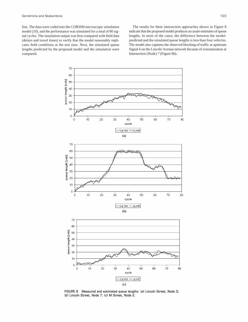
The results for three intersection approaches shown in Figure 8indicate that the proposed model produces accurate estimates of queuelengths. In most of the cases, the difference between the model-predicted and the simulated queue lengths is less than four vehicles.The model also captures the observed blocking of traffic at upstreamSignal 6 on the Lincoln Avenue network because of oversaturation atIntersection (Node) 7 (Figure 8b).

(a)

(b)

(c)

FIGURE 8 Measured and estimated queue lengths: (a) Lincoln Street, Node 3;(b) Lincoln Street, Node 7; (c) M Street, Node 2.

line. The data were coded into the CORSIM microscopic simulationmodel (10), and the performance was simulated for a total of 80 sig-nal cycles. The simulation output was first compared with field data(delays and travel times) to verify that the model reasonably repli-cates field conditions at the test sites. Next, the simulated queuelengths predicted by the proposed model and the simulation werecompared.

The proposed model formulation based on the LWR theory real-istically models the dispersion for both single and multiple platoonsalong arterials and explicitly considers the effect of residual queuesat oversaturated intersections on the estimation of traffic arrivals.

The proposed recursive formulation permits the prediction of thearrival profiles many signals downstream from a known starting flow.This output is an important tool for the estimation of queue lengthsand the prediction of link travel times even when the data from loopdetectors are unknown, inaccurate, or aggregated. Work is in progressto extend the model to optimize the offsets between intersections insignalized networks and to estimate the travel times in real time alongsignalized arterials (11).

ACKNOWLEDGMENTS

The study described in this paper was performed as part of the Cali-fornia’s Partners for Advanced Highways and Transit Program at theInstitute of Transportation Studies, University of California, Berke-ley. The authors thank Pravin Varaiya for comments and suggestionsthroughout the study.

REFERENCES

1. Denny, R. W., Jr. Traffic Platoon Dispersion Modeling. Journal of Trans-portation Engineering, Vol. 155, No. 2, 1989, pp. 193–207.

124 Transportation Research Record 1934

2. Pacey, G. M. The Progress of a Bunch of Vehicles Released from a Traf-fic Signal. Research Note Rn/2665/GMP. Road Research Laboratory,London, 1956.

3. Robertson, D. I. TRANSYT: A Traffic Network Study Tool. Road ResearchLaboratory Report LR 253. Road Research Laboratory, Crowthorne,United Kingdom, 1969.

4. Rouphail, N., A. Tarko, and J. Li. Traffic Flow at Signalized Inter-sections. In Revised Monograph on Traffic Flow Theory, Chapter 9,1992. http://www.tfhrc.gov/its/tft/tft.htm. Accessed 2003.

5. Rumsey, A. F., and M. G. Hartley. Simulation of a Pair of Intersections.Traffic Engineering & Control, Vol. 13, 1972, pp. 522–525.

6. Lighthill, M. J., and J. B. Whitham. On Kinematic Waves. I. Flow Move-ment in Long Rivers. II. A Theory of Traffic Flow on Long CrowdedRoad. Proceedings of the Royal Society, A, Vol. 229, 1955, pp. 281–345.

7. Richards, P. I. Shockwaves on the Highway. Operations Research, Part B,Vol. 22, 1956, pp. 81–101.

8. Highway Capacity Manual. TRB, National Research Council, Washing-ton, D.C., 2000.

9. Daganzo, C. F. Fundamentals of Transportation and Traffic Operations.Pergamon, Oxford, United Kingdom, 1997.

10. CORSIM User’s Manual. FHWA, U.S. Department of Transportation,2003.

11. Skabardonis, A., and N. Geroliminis. Real-Time Estimation of TravelTimes Along Signalized Arterials. Presented at 16th International Sym-posium on Transportation and Traffic Theory, University of Maryland,July 2005.

The contents of this paper reflect the views of the authors, who are responsible for the facts and the accuracy of the data presented here. The contents do not necessarily reflect the official views or policy of the California Department of Transportation. This paper does not constitute a standard, specification, or regulation.

The Traffic Flow Theory and Characteristics Committee sponsored publication ofthis paper.