Page 1
POLITECNICO DI MILANO
M.Sc. in Civil Engineering for Risk Mitigation
Prediction of Clear-water Local Scour at Bridge Piers
Supervisors
Dr. Alessio Radice
Prof. Silvio Franzetti
Thesis by
Seyed Kamran Jalali 780545
July 2014
Page 2
1
POLITECNICO DI MILANO
Prediction of Clear-water Local Scour at Bridge Piers
A Master thesis submitted to Department of Civil and Environmental Engineering in partial
fulfillment of the requirements for the degree of Master of Science in Civil Engineering for Risk
Mitigation.
Submitted by: Supervised by:
_________________ _________________
Seyed Kamran Jalali Dr. Alessio Radice
Student ID: 780545 Dept. of Civil and Environmental Engineering
Politecnico di Milano
Piazza L. da Vinci, 32, I-20133 Milan
Co-supervised by:
_________________
Prof. Silvio Franzetti
Dept. of Civil and Environmental Engineering
Politecnico di Milano
Piazza L. da Vinci, 32, I-20133 Milan
Page 3
2
Abstract (English)
The major damage to bridges at river crossings occurs during floods. Damage is caused by
various reasons, one of the main ones being riverbed scour at bridge foundations (piers and
abutments). The damage can range from minor erosion to complete failure of the bridge structure
or its road approach. Complete failure results in severe disruption to local traffic flows.
The localized scour phenomenon and specifically scour at bridge piers has been the subject
of extensive investigations by many researchers and vast literature exists on the topic. In spite of
this big research effort, comprehensive design approaches are still missing due to a general
inability of predictive equations to fit data from different authors. In this thesis, a relatively large
amount of local scour data (516 experiments) has been collected from literature works on clear-
water scour at cylindrical piers. A great deal of work has been devoted to selecting experiments
that were not evidently flawed by some irregularity that could be due to any problem occurred
during performance of the tests.
An appropriate dimensionless framework has been introduced to steer the following analysis
of literature scour values. It was recognized that different authors made different choices
performing their experiments, therefore one of the most important actions undertaken here has
been making all the tests homogeneous. The treatment of flow velocity was evidently a crucial
factor, thus it was considered with highest attention. In this context, an analysis of threshold
condition has been conducted to find a suitable criterion for defining a threshold for sediment
movement and the one proposed by Melville & Coleman (2000) was finally chosen as the most
suitable one among the other available criteria in literature. In this way the critical velocity for
sediment motion of all the experiments was computed by a unique criterion. On the other hand,
all the measured upstream flow velocities were unified by converting all the declared values by
the different authors to depth-averaged velocity at the channel axis. Thanks to these strategies, all
the experiments could be used as a unique, homogeneous database.
The dimensionless scour depth (the ratio between the scour depth and the pier diameter) was
investigated in terms of its dependence on flow intensity, sediment coarseness and
nondimensional time. A formula has been proposed for prediction of the scour depth. The
equation consists of an exponential factor for considering the effect of sediment coarseness and a
3rd
order polynomial for the effect of flow intensity; a multiplicative constant accounts for
different times. The proposed model is valid for a vast range of flow intensities (0.48 ≤ U ≤ 1.39)
and sediment coarseness ratios (2 ≤ D50 ≤ 325). Finally, the predictive capability of the present
formula has been shown to be better than those of existing literature approaches.
Author keywords: Bridge piers; Local scour; Scour prediction; Flow intensity; Sediment
coarseness; Temporal evolution.
Page 4
3
Abstract (Italian)
Durante gli eventi alluvionali i ponti fluviali possono essere significativamente danneggiati, o
anche distrutti, dai fenomeni di erosione localizzata alla base delle strutture in alveo (pile e
spalle), con evidenti conseguenze negative sul sistema viabilistico. I processi erosivi
rappresentano una delle cause di maggior rilievo di vulnerabilità dei ponti.
I processi erosive localizzati sono stati oggetto di una vasta ricerca negli ultimi decenni;
sfortunatamente, nonostante i notevoli sforzi profusi nello studio, gli strumenti per la previsione
della profondità di scavo ancora non consentono di condurre stime affidabili, stante la non
capacità delle formule proposte di rappresentare correttamente i dati dei vari autori. In questa tesi
sono stati considerati parecchi dati di letteratura (provenienti da 516 prove di laboratorio) relativi
all’erosione alle pile circolari in condizioni di acque chiare. La prima importante parte del lavoro
ha riguardato un’attenta selezione delle prove che potessero essere in qualche modo inficiate da
problematiche occorse durante l’esperimento, risultando in andamenti evidentemente irregolari.
Per l’analisi dei dati sperimentali è stato messo a punto un adeguato inquadramento
adimensionale. Riconoscendo che i diversi autori hanno svolto i propri esperimenti a partire da
scelte differenti, uno sforzo significativo è stato fatto per rendere i dati confrontabili tra loro. Un
aspetto cruciale è stato identificato nella maniera di trattare la velocità del flusso. È stata fatta in
primo luogo un’analisi della stima delle condizioni di incipiente movimento, a seguito della
quale si è deciso di considerare il criterio proposto da Melville & Coleman (2000) applicandolo a
tutti gli esperimenti. In secondo luogo, la velocità del flusso è stata sempre espressa in termini di
valore relativo all’asse del canale e mediato sulla verticale, effettuando le opportune conversioni
dalla velocità media sulla sezione quando necessario. In questa maniera è stato possibile
omogeneizzare i dati in maniera significativa.
È stata analizzata la dipendenza della profondità di scavo (adimensionalizzata sulla
dimensione della pila) rispetto alla velocità del flusso, alla dimensione dei sedimenti e al tempo,
arrivando a proporre una formula interpolare. L’equazione è composta da un contributo
esponenziale per la dimensione dei sedimenti, da un polinomio di terzo grado per l’effetto della
velocità del flusso, e da una costante moltiplicativa che tiene conto del tempo. La formula
proposta, che si è dimostrata avere un’affidabilità maggiore di quelle delle formule di letteratura
attualmente disponibili, è valida in un range i condizioni relativamente ampio (0.48 ≤ U ≤ 1.39; 2
≤ D50 ≤ 325).
Author keywords: Pila di ponte; Erosione localizzata; Previsione dell’erosione; Intensità di
trasporto; Sedimenti; Evoluzione temporale.
Page 5
4
Abstract (Persian)
برای بروز این خسارات وجود دارد، که دالیل متعددی در هنگام وقوع سیل اتفاق می افتد. ،های وارده به پلها عمده خسارت
می تواند وارده ت هایخسار شدت. به شمار می آیدترین آنها عمده از ( ودیواره ی پل پایه ها) پیبستر رودخانه در ناحیه آبشستگی
ترافیک منطقه شود. ختالل درا و در نهایت منجر به ایجادباشد متغییر کامل اسکلت پل تخریبتا ی و موضعجزئی آبشستگی از
و مقاالت متنوعی دراین تحقیق کرده اند پایه پلها تگیسآبشی و خصوصا موضع تگیسآبشپدیده ی محققان زیادی در مورد
، به علت عدم توانایی معادالت ارائه شده برای تخمین مقدار متعدد در این زمینه با وجود مطالعات .به چاپ رسیده استخصوص
اطالعات ارائه نشده است. در این پایان نامه طراحی جامعی برای روشکماکان داده های بدست آمده توسط دیگر محققان، تگیسآبش
وری آگرد ستونهای استوانه ای پیرامون در حالت آب زالل تگیسآبشاز مطالعات وآزمایشات گذشته در مورد آزمایش( ۶۱۵)زیادی
اجرا یا اندازه گیریدر تیمشکال وقوع ای از نشانه می تواند که، کامل زمانی نامنظم آبشستگیت باآزمایشات ،در این میان شده است.
.حذف شده اند، باشد
با توجه به است. از پارامترهای بی بعد صورت گرفتهبه کمک انتخاب ترکیب مناسبی ،دادهای بدست آمده از منابع متنوع تحلیل
از اهمیت خاصی برخوردار ات ز منابع مختلف، همگن سازی آزمایشای جمع آوری شده ااختالف های موجود در نحوه آزمایش داده
ی این پارامتر شده است. در این خصوص، برای زدر پدیده آبشستگی، توجه ویژهای به همگنسا جریان تسرعباالی ریثات به علت است.
ند. ه اای موجود در مقاالت مختلف مورد تحلیل قرار داده شد، معیارهبرای تخمینن آن مناسب روشرسوبات و تعیین حملتایین آستانه
به عنوان معیار برتر برای تخمین آستانه حمل رسوبات برگزیده و سپس (۰۲۲۲) کولمندر این میان معیار ارائه شده توسط ملویل و
تمامی مقادیر سرعت جریان اعالم از سویی دیگر، توسط این معیار بدست آورده شد. ،سرعت بحرانی تمام آزمایشات جمع آوری شده
شده توسط مولفان، به منظور یکپارچه سازی هر چه بیشتر داده ها، به سرعت متوسط عمقی در محور کانال تبدیل شدند. در نتیجه با
.نموداستفاده یک پایگاه داده واحد عنوان آزمایشات جمع آوری شده به می توان از توجه به استراتژی های اتخاذ شده،
عمق آبشستگی بدون بعد )نسبت بین عمق آبشستگی به قطر ستون( بر اساس وابستگی آن به شدت جریان، زبری رسوبات و زمان
عاملی نمایی برای در وسپس معادله ای برای تخمین عمق آب شستگی ارائه شد. این معادله شامل رار گرفتبدون بعد مورد بررسی ق
اثر زمانهای مختلف نیز به ؛ می باشدچند جمله ای درجه سه برای در نظر گرفتن اثر شدت جریان ری رسوبات و یکبنظر گرفتن اثر ز
۰٫۸۴ شدت جریاننسبت از یاست. مدل ارائه شده برای بازه وسعی به حساب آمدهکمک یک ضریب ثابت و زبری ۱٫۹۳
۲ رسوبات ائه شده نسب به مدلهای موجود در منابع نشان داده برتری مدل ار با کمک مقایسه صادق است. در نهایت، ۹۲۳
شده است.
.؛ شدت جریان؛ زبری رسوبات؛ تکامل زمانییموضع یکلید واژه ها: پایه پل؛ آبشستگ
Page 6
5
Acknowledgments
I would like to express my gratitude to my sincere supervisors, Professor Dr. Alessio Radice
and Prof. Silvio Franzetti for the constant and useful comments, remarks and engagement
through the learning process of this master thesis. I feel motivated and encouraged every time I
attend their meeting.
Many friends have helped me stay sane through these difficult years. Their support and care
helped me overcome setbacks and stay focused on my graduate study. I greatly value their
friendship and I deeply appreciate their belief in me.
Last, but not least, I would like to extend my deepest gratitude to my parents, my sister and
my brother without whose love, support and understanding I could never have completed this
master degree.
Seyed Kamran Jalali
Politecnico di Milano
July 2014
Page 7
6
List of Tables
Table 1.1: Basic bed forms in alluvial channels (classification by increasing flow velocities) ... 25
Table 2.1: Full trend data sources and number for each source. ................................................... 38
Table 2.2: Isolated points sources and number for each source. .................................................. 39
Table 2.3: Sediment properties used in Ettema (1980) experiment .............................................. 42
Table 2.4: Pier size used in Ettema (1980) experiment ................................................................ 42
Table 2.5: Ettema (1980) critical shear velocity definition .......................................................... 43
Table 2.6: Flow, sediment and structure parameters summary .................................................... 47
Table 2.7: The local scour results summary ................................................................................. 48
Table 2.8: VAW pier data- test conditions ................................................................................... 51
Table 2.9: VAW Pier Data- summary of test conditions .............................................................. 52
Table 2.10: Characteristic controlling variable of Lanca et al. (2013)’s experiment ................... 53
Table 2.11: Summary of Girmaldi (2005) and Simarro et al. (2011) experiment used for
validation....................................................................................................................................... 55
Table 2.12: Sediments characteristics ........................................................................................... 55
Table 2.13: Approach flow characteristics ................................................................................... 56
Table 2.14: Chabert, J. and Engeldinger, P. (1956) test characteristic summary ......................... 61
Table 2.15: Mignosa, P. (1980) test characteristic summary ........................................................ 62
Table 2.16: Franzetti et al (1989) and Azzaroli, D. (1983) tests characteristic summary ............ 64
Table 3.1: Ettema (1980) critical shear velocity definition .......................................................... 67
Page 8
7
List of Figures
Figure 1.1: Force acting on a sediment particle (inter-granular forces not shown) ...................... 17
Figure 1.2: Diagram of forces acting on a sediment particle in open channel flow (Yang, 1973) 18
Figure 1.3: Experimental data by Shields (1936) ......................................................................... 20
Figure 1.4: Shields diagram for incipient motion (Vanoni, 1975) ................................................ 21
Figure 1.5: Bed-load motion: (a) Sketch of saltation motion (b) definition sketch of bed-load
layer............................................................................................................................................... 22
Figure 1.6: Suspended-sediment motion by convection and diffusion processes. ....................... 24
Figure 1.7: Bed form is movable boundary hydraulics: (a) typical bed forms and (b) bed form
motion. .......................................................................................................................................... 24
Figure 1.8: Total scour and its components .................................................................................. 27
Figure 1.9: Schematic representation of scour at a cylindrical pier .............................................. 27
Figure 1.10: Diagrammatic Flow Pattern at Cylindrical Pier ....................................................... 28
Figure 1.11: (a) Time development of clear-water and live-bed scour (b) scour depth as a
function of shear velocity (after Chabert & Engeldinger 1956) ................................................... 29
Figure 2.1: Cross-section of the working section of 1.52 m wide, flow recirculating, flume by
Ettema (1980)................................................................................................................................ 40
Figure 2.2: Cross-section of the working section of the 0.46 m wide flume by Ettema (1980) ... 41
Figure 2.3: Digitization of Ettema (1980) sample ........................................................................ 44
Figure 2.4: Schematic drawing of flume used for Sheppard et al.’s (2002) research ................... 45
Figure 2.5: Isometric drawing of the flume .................................................................................. 46
Figure 2.6: Definition sketch and measurement points for: (a) pier and (b) abutment. Points
defining (●) scour or aggradation depths; (+) scour or aggradation area ..................................... 50
Figure 2.7: Evolution of dimensionless scour depth at pier nose under steady flow (Chang et al.
(2005))........................................................................................................................................... 56
Figure 2.8: Test flume, plan and profile ....................................................................................... 57
Figure 2.9: Scour data for cylindrical pier .................................................................................... 58
Figure 2.10: Uniform sediments size and gradations.................................................................... 59
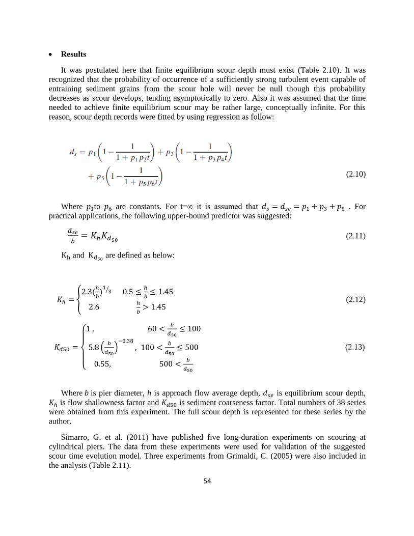
Figure 2.11: Test flume from Chabert and Engeldinger (1956) ................................................... 60
Figure 2.12: Scour depth with respect to time trend taken from Franzetti et al.’s (1981)
experiment..................................................................................................................................... 63
Figure 2.13: Scour depth with respect to time graph taken from Azzaroli, D.’s (1983) experiment
....................................................................................................................................................... 64
Figure 3.1: Comparison of different criteria for computing uc ..................................................... 70
Figure 3.2: Comparison of different criteria for computing uc* .................................................... 70
Figure 3.3: Comparison of different criteria for deriving shear critical stress with respect to
Shields experiments with Re* as x axis ........................................................................................ 71
Figure 3.4: Comparison of different criteria for deriving shear critical stress with D* as x axis . 71
Page 9
8
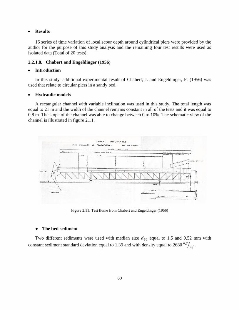
Figure 3.5: Comparison of measured and calculated values of velocity by means of conversion
formula by Paleari (2014) ............................................................................................................. 73
Figure 3.6: Local scour depth variations with respect to flow shallowness ................................. 74
Figure 3.7 : An example of test with regular trend ....................................................................... 76
Figure 3.8: Disregarded test from Mignosa (1980) and Ettema (1980) due to trend non-regularity
....................................................................................................................................................... 77
Figure 3.9: Selection procedure for dimensionless time, T, equal to 105 (a) and 10
6 (b) ............. 78
Figure 3.10: flow regime verification procedure .......................................................................... 79
Figure 3.11: The outcomes of regime verification. (a) For T= 5 (b) For T= 10
6 ....................... 79
Figure 3.12: presentation of valid tests for T=106 on moody diagram ......................................... 80
Figure 3.13: presentation of valid tests for T=105
on moody diagram ......................................... 80
Figure 3.14: Presentation of valid data for D50 with respect to U ................................................. 81
Figure 3.15: Presentation of valid data for H with respect to U ................................................... 82
Figure 3.16: Presentation of valid data Ds with respect to T ........................................................ 82
Figure 3.17: Presentation of valid data U with respect to T ......................................................... 83
Figure 3.18: Cumulative distribution function of u*/uc* for valid data ........................................ 83
Figure 3.19: Cumulative distribution function of dimensionless time for valid data ................... 84
Figure 3.20: Cumulative distribution function of Ds (ds/b) for valid data .................................... 84
Figure 3.21: Presentation of valid data at T=105 and T=10
6 in Shield Diagram .......................... 85
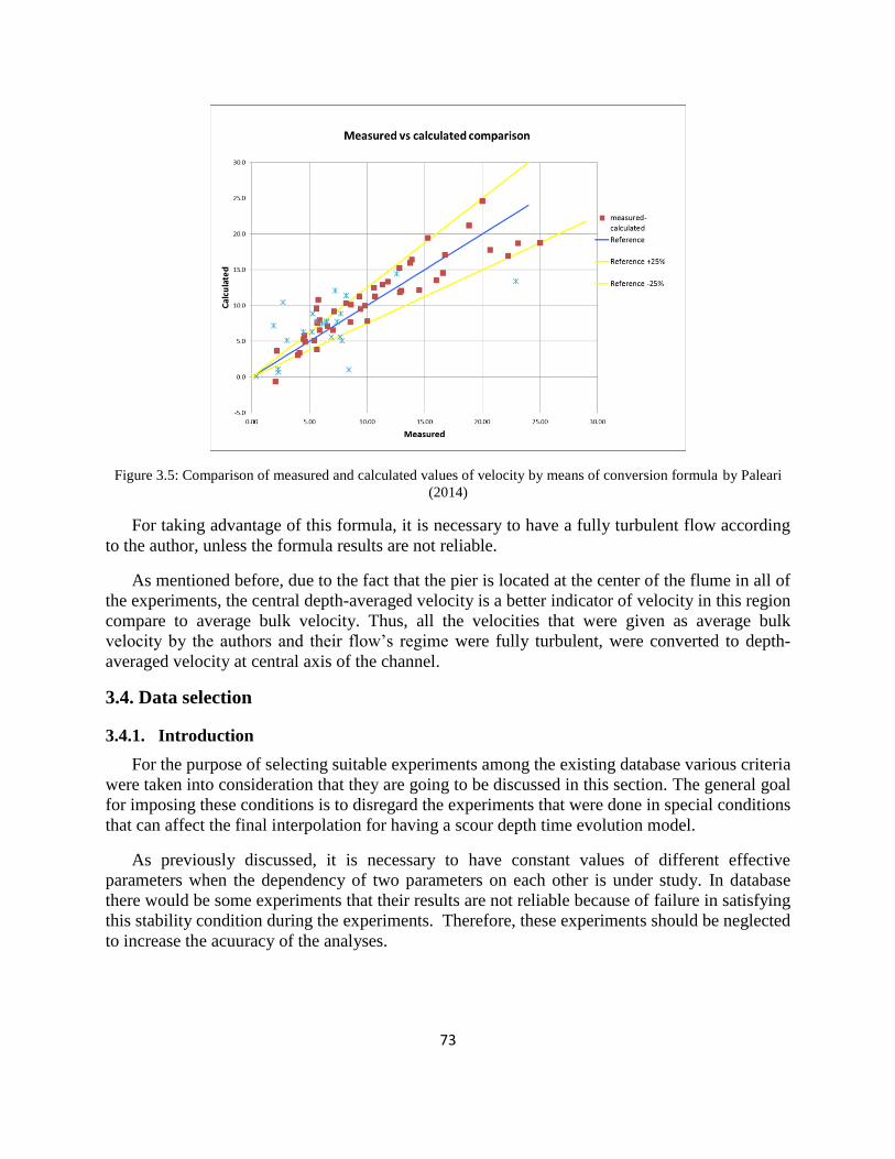
Figure 3.22: Example of interpolation for finding scour depth (ds) at requested nondimensional
time (T) ......................................................................................................................................... 86
Figure 3.23: presentation of accepted range and valid tests for assuming that the final scour depth
is equal to scour depth at T=106 for isolated points data .............................................................. 87
Figure 3.24: Ds with respect to D50 divided into groups of U (a) T=105 (b) T=10
6 ..................... 87
Figure 3.25: Ds with respect to U divided into groups of D50 (a) T=105 (b) T=10
6 ..................... 88
Figure 3.26: Valid data in Ds-D50 space for both T=105 and T=10
6 ............................................. 89
Figure 3.27: First attempt for f2 (D50) at T=106 (up) and T=10
5 (down) (0.8<U<1.2) ................. 90
Figure 3.28: First attempt for f3 (U) at T= 106 (up) and T= 10
5 (down) ....................................... 91
Figure 3.29: Calculated Vs. measured values of Ds at T=106 (left) and T=10
5 (right) for the first
attempt........................................................................................................................................... 92
Figure 3.30: f2 (D50) obtained from final attempt at T=106 (up) and T= 10
5 (down) ................... 93
Figure 3.31: Final attempt for obtaining f3 (U) with two different equation forms for T=106 (up)
and T=105 (down) ......................................................................................................................... 94
Figure 3.32: Comparison of proposed formulas with previous results in literature ..................... 95
Figure 3.33: Calculated Vs. measured values of Ds at T= 106 (up) and T=10
5 (down) for the final
attempt........................................................................................................................................... 96
Figure 3.34: Calculated Vs. measured values of Ds at T= 106 (up) and T=10
5 (down) using
Melville & Chiew (1999) .............................................................................................................. 98
Figure 3.35: Calculated Vs. measured values of Ds at T= 106 (up) and T=10
5 (down) using
Lanca, et al. (2013) ..................................................................................................................... 100
Page 10
9
Figure 3.36: Calculated Vs. measured values of Ds at T= 106 (up) and T=10
5 (down) using
Sheppard et al. (2014) ................................................................................................................. 101
Figure 3.37: Calculated Vs. measured values of Ds at T= 106 (up) and T=10
5 (down) using
Oliveto and Hager (2002) ........................................................................................................... 103
Figure 3.38: Calculated Vs. measured values of Ds at T= 106 (up) and T=10
5 (down) using
Oliveto and Hager (2002) and velocity proposed by the authors ............................................... 104
Page 11
10
List of Symbols
ρ: Density of water;
μ: Dynamic viscosity of water;
ν: Kinematic viscosity of water;
γ: Specific weight of water;
g: Acceleration of gravity;
Width of the channel;
h: Mean approach flow depth;
b: Width of the pier (Diameter of cylindrical pier);
Local scour depth at time t;
Local scour depth at equilibrium;
Median grain size;
σ: Standard deviation of sediment particle size distribution;
: Sediment density;
t: Time;
u: Mean approach flow velocity;
Mean approach flow velocity at threshold condition for sediment movement;
Shear velocity;
Critical shear velocity for sediment movement;
Hydraulic radius of channel;
Re: Reynolds number;
Particle Reynolds number;
Fr: Froude number;
Sediment coarseness (b/d50);
H: Flow shallowness (h/b);
Δ: Relative submerged weight of sediments;
Page 12
11
T: Dimensionless time (t.u/b);
U: Flow intensity (u/uc); and
: Dimensionless scour depth (ds/b).
Page 13
12
Contents
Abstract (English) ............................................................................................................ 2
Abstract (Italian) .............................................................................................................. 3
Abstract (Persian) ............................................................................................................. 4
Acknowledgments ............................................................................................................ 5
List of Tables .................................................................................................................... 6
List of Figures .................................................................................................................. 7
List of Symbols .............................................................................................................. 10
Introduction .................................................................................................................... 15
1. GENERAL DESCRIPTION & OBJECTIVES ..................................................................... 17
Sediment transport in open channels .............................................................................. 17 1.1.
Introduction ............................................................................................................. 17 1.1.1.
Incipient motion of sediments ................................................................................. 17 1.1.2.
Forcing action on sediment particle................................................................. 17 1.1.2.1.
Threshold of sediment movement ................................................................... 18 1.1.2.2.
Dimensional analysis ....................................................................................... 19 1.1.2.3.
Shileds diagram ............................................................................................... 19 1.1.2.4.
Sediment transport mechanism ............................................................................... 22 1.1.3.
Bed-load transport ........................................................................................... 22 1.1.3.1.
Bed-load transport rate .................................................................................... 23 1.1.3.2.
Suspended-load transport ................................................................................ 23 1.1.3.3.
Bed formation ......................................................................................................... 24 1.1.4.
Scour............................................................................................................................... 25 1.2.
An introduction to scour ......................................................................................... 25 1.2.1.
Contribution to total scour ...................................................................................... 26 1.2.2.
Aggradation and Degradation .......................................................................... 26 1.2.2.1.
General Scour (contraction scour & other general scour) ............................... 26 1.2.2.2.
Local scour ...................................................................................................... 26 1.2.2.3.
Lateral stream migration .................................................................................. 26 1.2.2.4.
Local scour ..................................................................................................................... 27 1.3.
Page 14
13
Local scour mechanism........................................................................................... 27 1.3.1.
Clear-water and Live-bed scour .............................................................................. 28 1.3.2.
The parameters of local scour at piers .................................................................... 30 1.3.3.
Dimensionless analysis of local Scour depth .......................................................... 31 1.3.4.
Some existing formula for evaluation of local scour .............................................. 33 1.3.5.
Objectives ....................................................................................................................... 37 1.4.
2. AVAILABLE DATA AND LITERATURE REVIEW ........................................................ 38
Introduction .................................................................................................................... 38 2.1.
Data Characteristics........................................................................................................ 39 2.2.
Full trend scour depth data ...................................................................................... 39 2.2.1.
Ettema (1980) .................................................................................................. 39 2.2.1.1.
Sheppard, et al. (2002) ..................................................................................... 45 2.2.1.2.
Oliveto and Hager (2002) ................................................................................ 49 2.2.1.3.
Lanca, et al. (2013) .......................................................................................... 52 2.2.1.4.
Change et al. (2004) ......................................................................................... 55 2.2.1.5.
Yanmaz and Altinbilek (1991) ........................................................................ 57 2.2.1.6.
Raikar and Dey (2005) .................................................................................... 59 2.2.1.7.
Chabert and Engeldinger (1956)...................................................................... 60 2.2.1.8.
Mignosa (1980)................................................................................................ 61 2.2.1.9.
Franzetti et al (1989) ........................................................................................ 63 2.2.1.10.
Azzaroli (1983) ................................................................................................ 63 2.2.1.11.
Isolated scour depth points...................................................................................... 64 2.2.2.
3. DATA ANALYSIS ............................................................................................................... 65
Introduction .................................................................................................................... 65 3.1.
Analysis of threshold conditions .................................................................................... 66 3.2.
Introduction ............................................................................................................. 66 3.2.1.
Introducing criteria under study .............................................................................. 66 3.2.2.
Comparisons of different criteria ............................................................................ 69 3.2.3.
Velocity Conversion formulas ....................................................................................... 72 3.3.
Data selection ................................................................................................................. 73 3.4.
Introduction ............................................................................................................. 73 3.4.1.
Page 15
14
Selection Criteria .................................................................................................... 74 3.4.2.
Flow regime verification ......................................................................................... 78 3.4.3.
Presentation of valid data ............................................................................................... 81 3.5.
Dispersion of valid data .......................................................................................... 81 3.5.1.
Valid data in Shields diagram ................................................................................. 84 3.5.2.
Dependency verification ................................................................................................ 85 3.6.
Interpolation with valid data .......................................................................................... 88 3.7.
Introduction ............................................................................................................. 88 3.7.1.
Initial attempt .......................................................................................................... 88 3.7.2.
Further attempts ...................................................................................................... 92 3.7.3.
Final attempt ........................................................................................................... 92 3.7.4.
Summary of final results ......................................................................................... 97 3.7.5.
Model comparison with previous studies ....................................................................... 97 3.8.
Melville & Chiew (1999) ........................................................................................ 97 3.8.1.
Lanca et al. (2013) .................................................................................................. 99 3.8.2.
Sheppard et al. (2014) ........................................................................................... 100 3.8.3.
Oliveto and Hager (2002) ..................................................................................... 102 3.8.4.
Conclusions .................................................................................................................. 106
Recommendations for further research ........................................................................ 107
References .................................................................................................................... 108
Appendix 1: Summary of full trends and isolated points scour depth data ................................ 111
Appendix 2: Interpolation further attempts................................................................................. 125
Page 16
15
Introduction
Scour is a natural phenomenon caused by the erosive action of the flowing water on the bed
and banks of river and channels. It is the removal of sediments around or near structures located
in flowing water. Erosion induces lowering of the riverbed level, with a tendency to expose the
foundations of a bridge. Such scour around pier and pile-supported structures and abutments can
result in structural collapse and loss of life and property. The construction of bridges in river and
channels can cause contraction in the waterway at the bridge cross section and, as a consequence,
gives rise to significant scour at that location. As the scour continuously progresses at the site, it
undermines the foundations of the structure leading to possible failure.
Many bridges failed around the world because of extreme scour around piers. Failure of
bridges due to scour at their foundations, considering both abutments and piers, is a common
occurrence. For example, a study of the US Federal Highway Administration in 1973 concluded
that of 383 bridge failures, 25% involved pier damage and 72% involved abutment damage.
Prediction of local scour holes at hydraulic structures plays an important role in their design
and especially in designing bridge structure. Excessive local scour can progressively make the
foundation of the structure weaker and lead to failure of the whole structure. Scour-induced
structural failure tends to occur suddenly and without prior warning. Thus, this type of bridge
failure threatens serious damage in terms of both economic cost and human life and may
severely disrupt traffic flows. Because complete protection against scour is too expensive,
generally, the maximum scour depth and the location of the hole have to be predicted to
minimize the risk of failure by having a suitable design for facing its series consequences.
The localized scour phenomenon has been the subject of extensive investigations and vast
literature exists on the topic. The main aim of this thesis is to investigate and analyze the
experimental data that are available in literature on the scour-depth evolution at circular piers.
Based on full time series (whenever available) and isolated scour depth points obtained in
experiments by several authors and by making them collapse in dimensionless form, an effort
has been made to find a predictive equation for scour depth in uniform sediments under clear-
water steady flow.
In chapter 1 some general explanation about fundamental subjects relevant to local scour
phenomena can be found. This chapter includes some essential information about sediments
transport mechanisms, threshold of incipient grain motion, different types of scour, local scour
mechanism due to acceleration of flow and resulting vortices. The chapter finally states the
general objectives of the work.
The literature experiments, from different authors, that are used in this thesis are presented in
chapter 2. The brief review mostly accounts for experimental procedures used, whose knowledge
is important understand limitations in experiment unification towards a comprehensive analysis.
In chapter 3, first the key aspects for experiments characterization are identified. A general
comparison of different criteria provided by various authors for the purpose of introducing a
suitable threshold of sediment movement is presented. This attempt was done based on the fact
Page 17
16
that, according to the critical analysis, velocity may be one of the most problematic factors for
unifying different experiments as one database. Thus it is necessary to define a unique criterion
for computing the velocity for inception of sediment movement for all of the experiments that
are going to be used in the analysis. A criterion was finally selected and applied to all the tests
under investigation. Afterwards, a strategy which was taken for unifying the velocity
measurement among different experiment is explained. The velocity measurement method
differs from one experiment to the other one and may be in term of average bulk velocity or
depth-averaged velocity. Therefore, for having an integrated database it was necessary to select a
suitable velocity measurement method from existing ones and convert velocities which had been
measured with a different method. Third, , the imposed restrictions and the motivation of
considering them for selecting appropriate tests are discussed. Fourth, The path that was taken
for deriving a predictive equation for scour depth is provided: the process of data clustering and
curve fitting based on the effective parameters is explained. Finally, the predictive capability of
the proposed formula is assessed in comparison with that of some of the existing ones in the
literature.
A summary of major outcomes and conclusions completes the work.
A summary of the data that have been used in this study can be found in Appendix 1. In
Appendix 2, more details are provided about the regression procedure towards the final
predictive equation.
Page 18
17
Chapter 1
1. GENERAL DESCRIPTION & OBJECTIVES
Sediment transport in open channels 1.1.
Introduction 1.1.1.
Waters flowing in natural streams and rivers have the ability to scour channel beds, to carry
particles (heavier than water) and to deposit materials, hence changing the bed topography. This
phenomenon is of great economical importance specially to predict the risks of scouring of
bridges.
The transported material is called the sediment load. Distinction is made between the bed
load and the suspended load. The bed load characterizes grains rolling, sliding or saltation along
the bed while suspended load refers to grains maintained in suspension by turbulence.
Incipient motion of sediments 1.1.2.
Forcing action on sediment particle 1.1.2.1.
For an open channel flow with a movable bed, the forces acting on each sediment particle are
(Figure 1.1):
the gravity force
the buoyancy force
the drag force
the lift force
the reaction forces of the surrounding grain,
Where is the volume of the particle, is a characteristic particle cross-sectional area,
and are the drag and lift coefficients, respectively, and V is a characteristic velocity next to
the channel bed. The gravity force and the buoyancy force act both in the vertical direction while
the drag force acts in the flow direction and the lift force in the direction perpendicular to the
flow direction.
Figure 1.1: Force acting on a sediment particle (inter-granular forces not shown)
Page 19
18
Threshold of sediment movement 1.1.2.2.
Incipient motion is important in the study of sediment transport, channel degradation, and
stable channel design. Due to the stochastic nature of sediment movement along an alluvial bed,
it is difficult to define precisely at what flow condition a sediment particle will begin to move.
Consequently, it depends more or less on an investigator's definition of incipient motion. They
use terms such as “initial motion,” “several grain moving,” “weak movement,” and “critical
movement!” In spite of these differences in definition, significant progress has been made on the
study of incipient motion, both theoretically and experimentally. Figure 1.2 shows the forces
acting on a spherical sediment particle at the bottom of an open channel. For most natural rivers,
the channel slopes are small enough that the component of gravitational force in the direction of
flow can be neglected compared with other forces acting on a spherical sediment particle. The
forces to be considered are the drag force lift force submerged weight and resistance
force . A sediment particle is at a state of incipient motion when one of the following
conditions is satisfied:
Figure 1.2: Diagram of forces acting on a sediment particle in open channel flow (Yang, 1973)
= (1.1)
= (1.2)
= (1.3)
Where = overturning moment due to and
= resisting moment due to and
Page 20
19
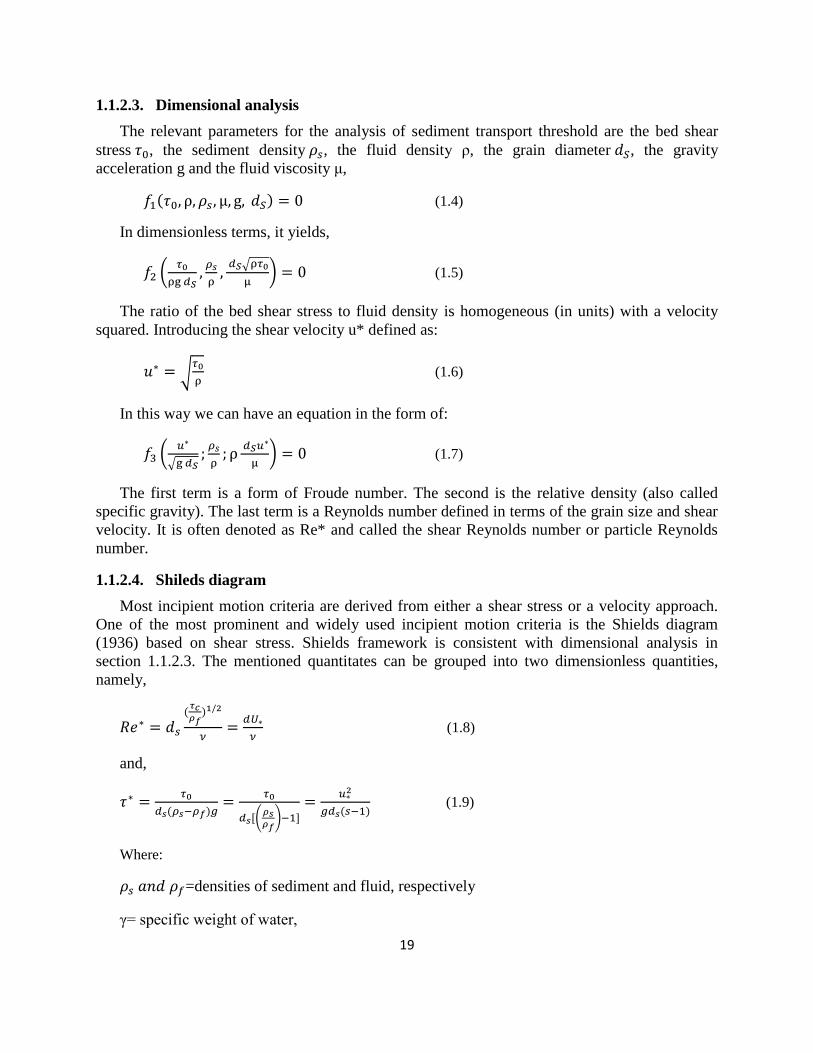
Dimensional analysis 1.1.2.3.
The relevant parameters for the analysis of sediment transport threshold are the bed shear
stress , the sediment density , the fluid density ρ, the grain diameter , the gravity
acceleration g and the fluid viscosity μ,
(1.4)
In dimensionless terms, it yields,
(
√
) (1.5)
The ratio of the bed shear stress to fluid density is homogeneous (in units) with a velocity
squared. Introducing the shear velocity u* defined as:
√
(1.6)
In this way we can have an equation in the form of:
(
√
) (1.7)
The first term is a form of Froude number. The second is the relative density (also called
specific gravity). The last term is a Reynolds number defined in terms of the grain size and shear
velocity. It is often denoted as Re* and called the shear Reynolds number or particle Reynolds
number.
Shileds diagram 1.1.2.4.
Most incipient motion criteria are derived from either a shear stress or a velocity approach.
One of the most prominent and widely used incipient motion criteria is the Shields diagram
(1936) based on shear stress. Shields framework is consistent with dimensional analysis in
section 1.1.2.3. The mentioned quantitates can be grouped into two dimensionless quantities,
namely,
(1.8)
and,
(
)
(1.9)
Where:
=densities of sediment and fluid, respectively
γ= specific weight of water,
Page 21
20
ν=fluid kinematic viscosity,
g=gravity,
=shear velocity, and
= stability parameter or shields parameter
= Shear Reynolds number
Critical value of the stability parameter may be defined at the inception of bed motion: i.e.
= (1.10)
Bed load motion occurs for:
> (1.11)
The relationship between these two parameters is then determined experimentally. Figure 1.3
shows the experimental data which was obtained by Shields during the experiment and Figure
1.4 shows the experimental results obtained by Shields and other investigators at incipient
motion. Any point in region above the curve indicates the situation of particle movement. In
region below the curve, the flow is unable to move the particles.
Figure 1.3: Experimental data by Shields (1936)
Page 22
21
Figure 1.4: Shields diagram for incipient motion (Vanoni, 1975)
Thus the critical shields parameter is:
(1.12)
And the critical grain Reynolds number is:
(1.13)
Where: Δ=
(1.14)
On the Shields diagram (Fig. 1.4), the Shields parameter and the particle Reynolds number
are both related to the shear velocity and the particle size. Some researchers proposed a modified
diagram: as a function of a dimensionless particle parameter . In this way, the above
equation can be manipulated and alternatively written as:
(1.15)
Page 23
22
Where is the dimensionless sediment size defined as:
√ ⁄
√
(1.16)
The second equation is usually preferred to original one because the critical shear stress
appears only in one dimensionless parameter.
Sediment transport mechanism 1.1.3.
There are two types of sediment transport mechanisms. Transported sediment material that is
maintained in suspension and sediment material transported by rolling, sliding and saltation
motion along the bed.
Bed-load transport 1.1.3.1.
When the bed shear stress exceeds a critical value, sediments are transported in the form of
bed load and suspended load. For bed-load transport, the basic modes of particle motion are
rolling motion, sliding motion and saltation motion. (Figure 1.5)
Figure 1.5: Bed-load motion: (a) Sketch of saltation motion (b) definition sketch of bed-load layer
The sediment transport rate may be measured by weight (units: N/s), by mass (units: kg/s) or
by volume (units: /s). In practice the sediment transport rate is often expressed by meter width
and is measured either by mass or by volume. These are related by:
(1.17)
Where is the mass sediment flow rate per unit width, is the volumetric sediment discharge
per unit width and is the specific mass of sediment.
Page 24
23
Bed-load transport rate 1.1.3.2.
The bed-load transport rate per unit width may be defined as:
(1.18)
Where is the average sediment velocity in the bed-load layer (Fig.1.5 (b)). Physically the
transport rate is related to the characteristics of the bed-load layer; its mean sediment
concentration , its thickness s, which is equivalent to the average saltation height measured
normal to the bed, and the average speed of sediment moving along the plane bed.
Suspended-load transport 1.1.3.3.
The other type of sediment transport mechanism is suspended-load transport. Although this
type of sediment transport mechanism is not too relevant with the topic of this study, but it will
be briefly discussed in this section for the sake of completeness.
Sediment suspension can be described as the motion of sediment particles during which the
particles are surrounded by fluid. The grains are maintained within the mass of fluid by turbulent
agitation without (frequent) bed contact. Sediment suspension takes place when the flow
turbulence is strong enough to balance the particle weight. The amount of particles transported
by suspension is called the suspended load.
The transport of suspended matter occurs by a combination of advective turbulent diffusion
and convection. Advective diffusion characterizes the random motion and mixing of particles
through the water depth superimposed to the longitudinal flow motion. In a stream with particles
heavier than water, the sediment concentration is larger next to the bottom and turbulent
diffusion induces an upward migration of the grains to region of lower concentrations. A time-
averaged balance between settling and diffusive flux derives from the continuity equation for
sediment matter:
(1.19)
Where is the local sediment concentration at a distance y measured normal to the channel
bed, is the sediment diffusivity and is the particle settling velocity. Sediment motion by
convection occurs when the turbulent mixing length is large compared to the sediment
distribution length scale. Convective transport may be described as the entrainment of sediments
by very large scale vortices: e.g. at bed drops, in stilling basins and hydraulic jumps (Fig 1.6).
Page 25
24
Figure 1.6: Suspended-sediment motion by convection and diffusion processes.
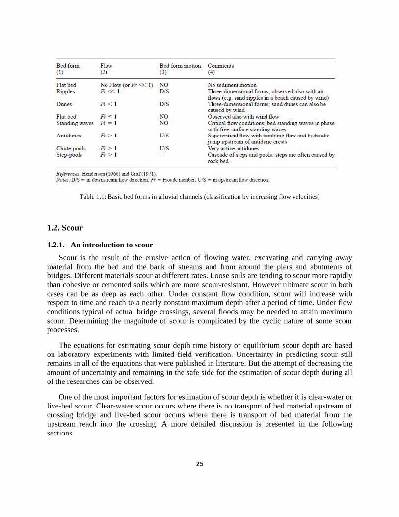
Bed formation 1.1.4.
In most practical situations, the sediments behave as a non-cohesive material (e.g. sand and
gravel) and the fluid flow can distort the bed into various shapes. The bed form results from the
drag force exerted by the bed on the fluid flow as well as the sediment motion induced by the
flow onto the sediment grains. This interactive process is complex.
The basic bed forms which may be encountered are the ripples (usually of heights less than
0.1 m), dunes, flat bed, standing waves and antidunes. The typical bed forms are summarized in
Figure 1.7 and Table 1.1.
Figure 1.7: Bed form is movable boundary hydraulics: (a) typical bed forms and (b) bed form
motion.
Page 26
25
Table 1.1: Basic bed forms in alluvial channels (classification by increasing flow velocities)
Scour 1.2.
An introduction to scour 1.2.1.
Scour is the result of the erosive action of flowing water, excavating and carrying away
material from the bed and the bank of streams and from around the piers and abutments of
bridges. Different materials scour at different rates. Loose soils are tending to scour more rapidly
than cohesive or cemented soils which are more scour-resistant. However ultimate scour in both
cases can be as deep as each other. Under constant flow condition, scour will increase with
respect to time and reach to a nearly constant maximum depth after a period of time. Under flow
conditions typical of actual bridge crossings, several floods may be needed to attain maximum
scour. Determining the magnitude of scour is complicated by the cyclic nature of some scour
processes.
The equations for estimating scour depth time history or equilibrium scour depth are based
on laboratory experiments with limited field verification. Uncertainty in predicting scour still
remains in all of the equations that were published in literature. But the attempt of decreasing the
amount of uncertainty and remaining in the safe side for the estimation of scour depth during all
of the researches can be observed.
One of the most important factors for estimation of scour depth is whether it is clear-water or
live-bed scour. Clear-water scour occurs where there is no transport of bed material upstream of
crossing bridge and live-bed scour occurs where there is transport of bed material from the
upstream reach into the crossing. A more detailed discussion is presented in the following
sections.
Page 27
26
Contribution to total scour 1.2.2.
Total scour at a bridge crossing considers three primary components:
Long-term degradation of the river bed;
General scour at bridge: a. Contraction scour b. Other general scour,
Local scour at the piers and abutments.
Total scour and its components are illustrated in figure 1.8.
Aggradation and Degradation 1.2.2.1.
Aggradation and degradation are long-term elevation changes due to the natural or man-
induced causes which can be affect the reach of the river on which the bridge is located.
Aggradation involves the deposition of material eroded from the channel or watershed upstream
of the bridge; whereas, degradation involves the lowering or scouring of the streambed due to a
lack in sediment supply from upstream.
General Scour (contraction scour & other general scour) 1.2.2.2.
General scour is a lowering of the streambed across the stream or waterway bed at bridge.
This lowering may be uniform across the bed or non-uniform, that is, the depth of scour may be
deeper in some part of the cross section. General scour may result from contraction of the flow,
which results in removal of material from the bed across all or most of the channel width, or
from other general scour conditions such as flow around a bend where the scour may be
concentrated near the outside of the bend. General scour is different from long-term degradation
in that general scour may be cyclic and/or related to the passing of a flood.
Local scour 1.2.2.3.
Local scour, which is the target of this study specifically among other types of scour,
involves removal of material from around piers, abutments, spurs, and embankments. It is caused
by an acceleration of flow and resulting vortices induced by obstruction to the flow. Local scour
can be either clear-water or live-bed scour. Local scour may occur even where general and
constriction scour are not present.
Lateral stream migration 1.2.2.4.
In addition to the types of scour mentioned above, naturally occurring lateral migration of the
main channel of a stream within a floodplain may affect the stability of piers in a floodplain,
erode abutments or the approach roadway, or change the total scour by changing the flow angle
of attack at piers and abutments. Factors that affect lateral stream movement also affect the
stability of a bridge foundation. These factors are the geomorphology of the stream, location of
the crossing on the stream, flood characteristics, and the characteristics of the bed and bank
materials.
Page 28
27
Figure 1.8: Total scour and its components
Local scour 1.3.
The following section provides more detailed discussion of the local scour at piers which is
the main goal of this research.
Local scour mechanism 1.3.1.
The basic mechanism causing local scour at piers or abutments is the formation of vortices
(known as the horseshoe vortex) at their base (Figure 1.9). The horseshoe vortex results from the
pileup of water on the upstream surface of the obstruction and subsequent acceleration of the
flow around the nose of the pier or abutment.
Figure 1.9: Schematic representation of scour at a cylindrical pier
Page 29
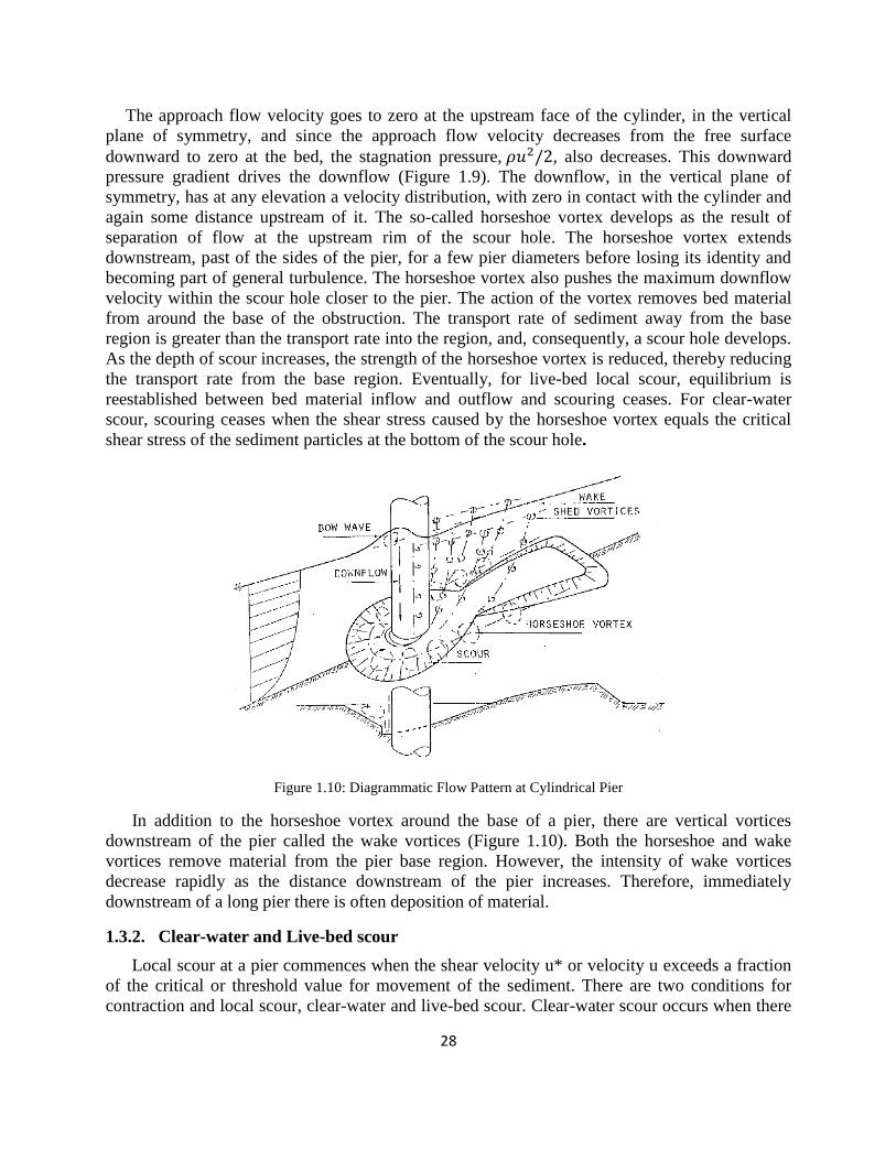
28
The approach flow velocity goes to zero at the upstream face of the cylinder, in the vertical
plane of symmetry, and since the approach flow velocity decreases from the free surface
downward to zero at the bed, the stagnation pressure, , also decreases. This downward
pressure gradient drives the downflow (Figure 1.9). The downflow, in the vertical plane of
symmetry, has at any elevation a velocity distribution, with zero in contact with the cylinder and
again some distance upstream of it. The so-called horseshoe vortex develops as the result of
separation of flow at the upstream rim of the scour hole. The horseshoe vortex extends
downstream, past of the sides of the pier, for a few pier diameters before losing its identity and
becoming part of general turbulence. The horseshoe vortex also pushes the maximum downflow
velocity within the scour hole closer to the pier. The action of the vortex removes bed material
from around the base of the obstruction. The transport rate of sediment away from the base
region is greater than the transport rate into the region, and, consequently, a scour hole develops.
As the depth of scour increases, the strength of the horseshoe vortex is reduced, thereby reducing
the transport rate from the base region. Eventually, for live-bed local scour, equilibrium is
reestablished between bed material inflow and outflow and scouring ceases. For clear-water
scour, scouring ceases when the shear stress caused by the horseshoe vortex equals the critical
shear stress of the sediment particles at the bottom of the scour hole.
Figure 1.10: Diagrammatic Flow Pattern at Cylindrical Pier
In addition to the horseshoe vortex around the base of a pier, there are vertical vortices
downstream of the pier called the wake vortices (Figure 1.10). Both the horseshoe and wake
vortices remove material from the pier base region. However, the intensity of wake vortices
decrease rapidly as the distance downstream of the pier increases. Therefore, immediately
downstream of a long pier there is often deposition of material.
Clear-water and Live-bed scour 1.3.2.
Local scour at a pier commences when the shear velocity u* or velocity u exceeds a fraction
of the critical or threshold value for movement of the sediment. There are two conditions for
contraction and local scour, clear-water and live-bed scour. Clear-water scour occurs when there
Page 30
29
is no movement of the bed material in the flow upstream of the crossing or the bed material
being transported in the upstream reach is transported in the suspension through the scour hole at
the pier or abutment at less than the capacity of the flow. In clear water condition velocity is
below the critical velocity and there is no sediment transport and no sediment supply into the
scour hole from upstream .At the pier or abutment the acceleration of the flow vortices created
by these obstructions cause the bed material around them to move. Live-bed scour occurs when
there is transport of bed material around them to move. Live-bed local scour is cyclic in nature;
that is, the scour hole that develops during the rising stage of a flood refills during falling stage.
Typical clear-water scour situation (1) coarse-bed material streams, (2) flat gradient streams
during low flow, (3) local deposition of larger bed materials that are larger than the biggest
fraction being transported by the flow (rock riprap is a special case of this situation), (4) armored
streambeds where the only location that tractive forces are adequate to penetrate the armor layer
are at piers and/or abutments, and (5) vegetated channel or overbank areas.
During a flood event, bridge over streams with coarse-bed material are often subjected to
clear-water scour at low discharge, live-bed scour at the higher discharges and clear-water scour
at low discharges on the falling stages. Clear-water scour reaches its maximum over a longer
period of time than live-bed scour (Figure 1.11). In fact, local clear-water scour may not reach a
maximum until after several floods and reach to its equilibrium asymptotically over a period of
days. Live-bed scour develops rapidly and its depth fluctuates in response to the passage of bed
features. (Figure 1.11(a)). This is due to the variability of the bed material sediment transport in
the approach flow when the bed configuration of the stream is dunes. Shen et al. (1969)
suggested that the mean value of the live-bed scour depth was about 10% less than the maximum
clear-water scour depth (Figure 1.11(b)).
Figure 1.11: (a) Time development of clear-water and live-bed scour (b) scour depth as a function of shear velocity
(after Chabert & Engeldinger 1956)
Critical velocity equations with the reference particle size equal to can be used to
determine the velocity associated with the initiation of motion. They are used as an indicator for
clear-water or live-bed scour conditions. If the mean velocity (u) in the upstream reach is equal
to or less than the critical velocity ( ) of the median diameter ( ) of the bed material, then
Page 31
30
contraction and local scour will be clear-water scour. If the mean velocity is greater than the
critical velocity of the median bed material size, live-bed scour will occur.
The parameters of local scour at piers 1.3.3.
Factors which affect the magnitude of local scour depth at piers can be stated as a general
function of fluid, flow, pier and sediment properties and time evolution.
Fluid: In mechanics a fluid is defined by its density ρ, kinematic viscosity ν, at temperature T.
Flow: The flow of a fluid is determined by its mean depth h, energy slope , and the
acceleration due to gravity g which generates the flow. The slope , which produces through the
component of gravity the shear stress, τ, to maintain the flow, is more suitably replaced by the
shear velocity √
Flow velocity also affects local scour depth. The greater the velocity, the deeper the scour will
be. There is a high probability that scour is affected by whether the flow is subcritical or
supercritical. However, most research data are for subcritical flow (i.e., flow with a Froude
Number less than 1.0, Fr < 1).
Pier: The action of pier is determined by the effective blockage it presents to the flow. A
cylindrical pier is defined by its diameter b. Other shaped piers are specified relative to b in
terms of shape factors. Consideration also can be made by introducing some factors for the angle
of the approach flow to the pier. As pier width increases, there is an increase in scour depth.
There is a limit to the increase in scour depth as width increases.
Pier length has no appreciable effect on local scour depth as long as the pier is aligned with the
flow. When the pier is skewed to the flow, the pier length has a significant influence on scour
depth. For example, doubling the length of the pier increases scour depth from 30 to 60 percent
(depending on the angle of attack).
Sediment: A layer of uniform cohesionless bed material of specific thickness is described by
the specific gravity and the sieve diameter of its particles. The degree of uniformity of particle
size distribution of a sediment is defined by the value of its standard deviation, σ. The most
common and convenient measure of standard deviation used in studies of the distribution of
particle size of a sediment is the graphic standard deviation, which is derive by reading two
values on the cumulative particle size curve,
=
(1.20)
The inclusive graphic standard deviation of Folk (1968) gives a better measure of the uniformity
of a sediment as it embraces 90 percent of distribution which is used in some of the studies:
=
(1.21)
Page 32
31
According to Ettema (1980), bed material in the sand-size range has little effect on local
scour depth. Likewise, larger size bed material that can be moved by the flow or by the vortices
and turbulence created by the pier or abutment will not affect the maximum scour, but only the
time it takes to attain it. Very large particles in the bed material, such as coarse gravels, cobbles
or boulders, may armor the scour hole. Fine bed material (silts and clays) will have scour depths
as deep as sand-bed streams. This is true even if bonded together by cohesion. The effect of
cohesion is to influence the time it takes to reach maximum scour. With sand-bed material the
time to reach maximum depth of scour is measured in hours and can result from a single flood
event. With cohesive bed materials it may take much longer to reach the maximum scour depth,
the result of many flood events.
Bed configuration of sand-bed channels affects the magnitude of local scour. In streams with
sand-bed material, the shape of the bed (bed configuration) may be ripples, dunes, plane bed and
etc. The bed configuration depends on the size distribution of the sand-bed material, hydraulic
characteristics, and fluid viscosity. The bed configuration may change from dunes to plane bed
during an increase in flow for a single flood event. It may change back with a decrease in flow.
The bed configuration may also change with a change in water temperature or suspended
sediment concentration of silts and clays. The type of bed configuration and change in bed
configuration will affect flow velocity, sediment transport, and scour.
Time: Scour is a dynamic process which seeks to establish a new equilibrium, between the
flow of the fluid and the resistance to motion of the bed particles, by the erosion of the flow
boundary; the local scour deepens progressively with time.
In summary, the down-flow impingement on the bed, along with the wide range of
turbulence structures present in the flow field, entrain and transport material from the scour hole.
The details and interaction of the flow field vary with pier characteristics such as shape, angle of
attack, and the stage of scour development between initiation and equilibrium, but the essential
consideration is that these flow features are responsible for scour.
Dimensionless analysis of local Scour depth 1.3.4.
The large number of interacting parameters makes the analysis of local scour at bed sediment
around a bridge pier very difficult. This has forced the researchers to use of dimensional
analysis. However the dimensional analysis is only a technique for grouping of variables, and
yields in itself no information. The relation between the depth of local scour at a bridge pier ,
and its dependent parameters can be written:
(1.22)
Where,
;
= fluid dynamic viscosity;
= mean approach flow depth;
Page 33
32
= acceleration of gravity;
= mean approach flow velocity;
= median size;
;
;
;
; and
.
An expression for the depth of local scour at a cylindrical pier of diameter b can be written as
a combination of dimensionless parameters:
√
(1.23)
Where we can substitute these terms by consider the following definitions:
Considering Reynolds number (Re) that is being used as a criterion to distinguish between
laminar and turbulent flow and is a measure of the ratio of the inertia force on an element of fluid
to the viscous force on an element and is equal to:
(1.24)
Where l is a characteristic length. Thus, particle Reynolds number can be written as:
√
(1.25)
Froude number (Fr) is also defining as a measure of the ratio of the inertia force on an
element of fluid to the weight of the element and it is equal to:
√ (1.26)
As mentioned before, the Shield diagram defines a for a given d50. A corresponding uc
can be found for the given flow depth, and thus the Froude number can be written, using the
given data as u/uc.
Page 34
33
Thus the equation (1.23) can be rewritten as:
(1.27)
The density ratio is assumed constant, and the Reynolds number influences are assumed
negligible for the highly turbulent flows envisaged. On the other hand, the effect of width of the
flow, in wide flows can be neglected and also by considering uniform sediment it is possible
to disregard the dependency to . Therefore, the other form which can represent the scour depth
as the function of dimensionless parameters is:
(1.28)
Where:
The functional relationships between dimensionless variables have to be obtained from
experiments, but when the number of dimensionless numbers is large severe experimental
problems occur. In this way the relationship between the four parameters mentioned above can
be obtained by less effort and in a more economical manner.
Some existing formula for evaluation of local scour 1.3.5.
In literature, it is possible to find several empirical or semi-empirical formulas for the
determination of the scour depth at equilibrium condition (final stage) or with respect to time
evolution. The differences in theses formulas are mostly due to their various experimental
conditions. Moreover, the validity range of existing formulas in literature is not similar for all of
them. This is the consequence of the difference in selection of the under consideration range for
dependent parameters of these studies. In addition, it is necessary to have constant values of
different effective parameters when the dependency of two parameters on each other is under
study. In some cases the mentioned required stability condition is failed and put a negative
effect on the accuracy of the final proposed formula. This dispersion in resulting formula by
different authors shows that scour depth determination is not clearly defined yet.
Each formula is only valid for the limited range of the author’s studies and cannot be
extended to other conditions such as different pier size, river width and flow velocity outside of
the mentioned range by the author.
In literature there are many authors who have expressed the dimensionless Scour depth as
a function of multiplication of different factor in which each of them take into account the
dependency of specific parameter. One of the most relevant combinations is as below:
(1.29)
Where define empirically through interpolation of the results usually
independently. It should be noted that, other factors rather than those mentioned here also can be
considered.
Page 35
34
Below, they are few definitions of the mentioned factors define by various authors:
Franzetti et al (1994)
0.67 ≤ U≤ 1
H≥ 2
Chiew (1995)
3.77 U-1.13 0.3 ≤ U≤ 1
1 ≤ ≤ 50
1 50
0 3
1 3
Dey et al. (1999)
0.42 ≤ U ≤ 1
Melville and Chiew (1999)
U < 1
U > 1
2.4 H H 0.7
0 5
H 5
Page 36
35
25
1 25
[ |
(
)|
]
Oliveto and Hager (2002)
Sheppard (2002)
Chang et al (2004)
0.4 U
- 0.034
1
= Obtain by a graph
Page 37
36
Sheppard et al (2004)
Raikar and Dey (2005)
9 ≤25
Obtain from graph
Lanca et al. (2013)
Where:
Page 38
37
Objectives 1.4.
The objectives of this research work can be summarized as below:
Collection of clear-water scour data for cylindrical piers from reliable sources in
literature;
Selection of long-duration, suitable and reliable data from previous research and
experiments by imposing appropriate selection criteria;
Homogenization of the available data, particularly by an analysis of threshold
conditions to choose a suitable criterion to be applied to all the experiments for
defining the threshold for inception of bed material motion;
Investigation of the effect of nondimensional time, T (t.u/b), sediment coarseness,
(b/ ), and upstream flow intensity, U (u/ ), on the scour depth;
Regression-based calibration of a predictive formula;
Comparison of the final proposed equation with several previous ones available in
the literature.
Page 39
38
Chapter 2
2. AVAILABLE DATA AND LITERATURE REVIEW
Introduction 2.1.
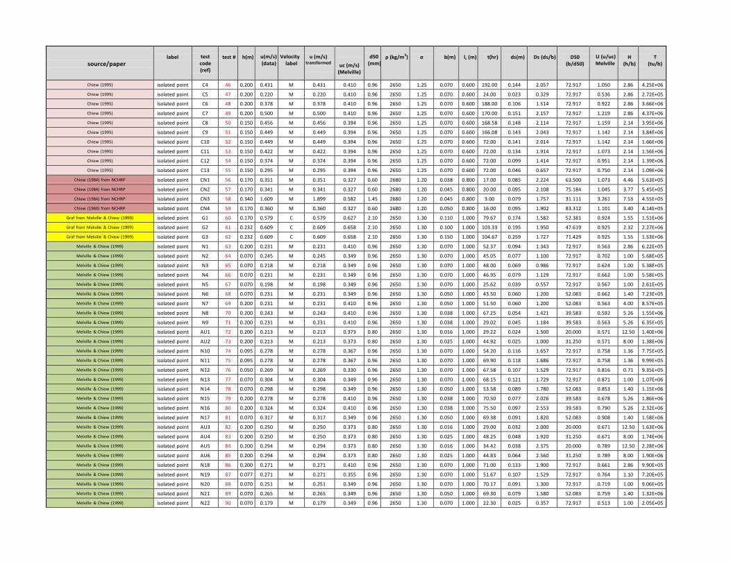
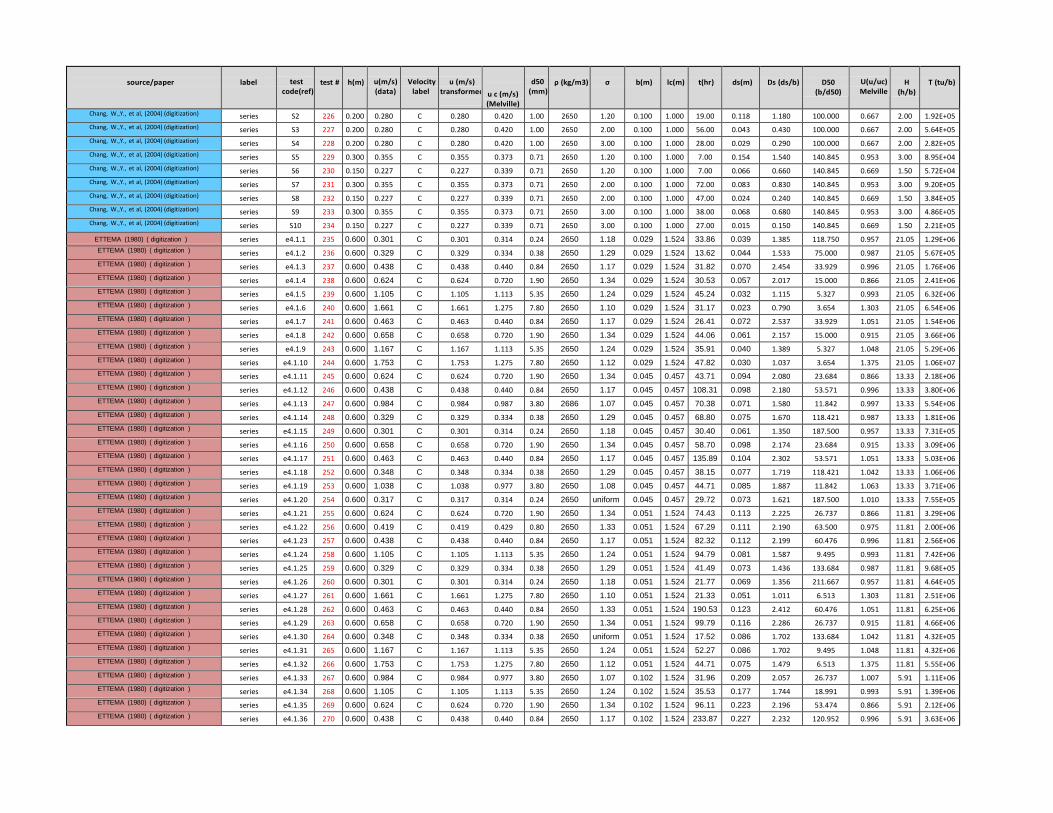
Relatively large quantities of local scour data have been used for the purpose of the analysis.
The sources and quantities of these data are listed in table 2.1 and 2.2. Laboratory data are
derived from experiments that were carefully performed and all the dependent parameters are
given by the author.
A total number of 516 experiments were used in this study. The data that have been
employed can be divided into two general categories:
1. Full trend scour depth data (324 experiments); which are the experiments where the full
scour depths evolution from the beginning of the experiments until the experiments stops, with
respect to time, were reported by authors. (Table2.1)
2. Isolated scour depth points (192 experiments); which are the data where only final or
maximum scour depth is provided by the authors and the time history of the scour holes
evolution were not reported or measured. (Table 2.2)
Main characteristics of data sources are given in the following section.
Table 2.1: Full trend data sources and number for each source.
Sources number of data
Ettema (1980) 105
Sheppard et al. (2002) 14
Oliveto and Hager (2002) 88
Lanca et al. (2013) 46
Chang et al. (2004) 10
Yanmaz and Altinbilek (1991) 18
Raikar and Dey (2005) 16
Chabert and Engeldinger (1952) 12
Mignosa (1979/1980) 13
Franzetti (1989) 1
Azzaroli (1983) 1
Total number of series 324
Full trend scour depth data
Page 40
39
Table 2.2: Isolated points sources and number for each source.
Data Characteristics 2.2.
In this section a brief summary about the experiments done by the various authors and the
aim and an achievement of their study is provided to have a better understanding about the data
that are going to be used in this study. For employing different experiment results from various
sources it is necessary to understand the assumptions which have been made. In this way, it is
possible to use these experiments as a unique database and attempt to make all of them
homogenous via analysis. It should be remembered that, all the collected experiments are in
clear-water condition according to authors report.
Full trend scour depth data 2.2.1.
Ettema (1980) 2.2.1.1.
Introduction and objectives
The aim of this project was to investigate experimentally the development of local scour in
uniform and non-uniform sediments as well as in beds formed of layers of uniform sediments. It
was hoped that each set of experiments would lead to recommendation for design of bridge piers.
Three main series of experiments were augmented.
In all the experiments cylindrical piers were used. The approach flow was steady for all
experiments.
Sources number of data
Yanmaz, Altinbilek (1991) 15
Melville and Chiew (1992) 27
Chiew (1995) 13
Chiew (1984) from NCHRP 4
Graf from Melville and Chiew (1999) 3
Melville and Chiew (1999) 51
Melville and Chiew (1999) from NCHRP 17
Dey et al (1995) 18
Ettema, RAUD 1
Ettema (1980) from NCHRP 2
Ettema, Kirkil and Muste (2006) 6
Sheppard and Miller (2006) 24
Raikar and Dey (2005) 4
Lee and Sturm (2009) 4
Ettema (1980) 3
Total number of points 192
Isolated scour depth points
Page 41
40
For the purpose of this study the experiments related to local scour of uniform sediment
around a pier were used. The stage of particle motion, expressed in terms of shear velocity
parameter / , was set on that all the experiments were performed at clear water local scour.
The experimental study was conducted in two parts:
The first part investigated the temporal development of local scour for a range of bed particle
sizes and cylindrical pier diameter, at similar values of the shear velocity parameter / with
different value of 0.95, 0.9, 0.75 or 0.5 at the center line of the approach flow. Two different
flumes were used in this study. The greater part of the study was performed in a 1.52 m wide re-
circulating flume for which the approach flow depth was kept constant at 0.6 m. Additional
experiments were conducted in a 0.46 m wide flume with flow provided by an outlet pipe from
the ring-main system of the laboratory with constant approach flow equal to 0.2 m for these
experiments.
The second parts was concerned with the influence of the approach flow depth, h by
Ettema notation), on the development of local scour at a cylindrical pier found in uniform
sediment. Shear velocity parameter was held constant at / = 0.9, at the center line of the
approach flow to the pier. The experiments were carried out in the 1.52 m wide flume. Three
piers sizes and three uniform bed sediments were used to investigate the influences of flow
depth, as well as that of pier and particle sizes, on the development of local scour.
Hydraulic Models
Most of the experiments on the temporal development of local scour were carried out in a
1.52 m wide, 1.22 m deep, glass-sided flume of approximately 45 m length (Figure 2.1). The
flow through the flume was re-circulated by two variable speed axial flow pumps driven by
thyristor controlled electric motors. In all experiments the flume slope was adjusted to ensure
that the depth of the flow was constant over the full length of the working section.
Figure 2.1: Cross-section of the working section of 1.52 m wide, flow recirculating, flume by Ettema (1980)
Page 42
41
The working section of the flume commenced at 20 m from the upstream end of the flume. It
consisted of an 8 m length false floor, upstream of 1.5 m wide and 3 m long sediment recess, in
which the pier was placed.
The approach bed roughness was simulated with the use of roughened sheet metal covers
which were fixed to the false floor. A selection of roughened sheets was made to cover the range
of sediment sizes used in the study.
An additional series of experiments was performed in a smaller glass-sided flume 0.456 m
wide, 0.44 m deep and approximately 19 m in length, served with water circulation system of the
laboratory. The water level in the flume was controlled by a tail gate. The roughness of the
approach bed was simulated in a similar manner to that described for the approach bed in 1.52 m
wide flume (Figure 2.2).
Figure 2.2: Cross-section of the working section of the 0.46 m wide flume by Ettema (1980)
The bed sediments
Sediment properties used in this experiment are listed in Table (2.3) where is mean
particle size of uniform sediments, and are two measurements of standard deviation of
particle size distribution of each bed sediments ( <1.5 may be considered as being virtually of a
uniform particle size. All of the eight bed sediment that used in this experiments fulfill this limit
so they can be considered as uniform sediments.), is specific gravity, is critical shear
velocity and computed by using shields function. S.F is particle shape factor which has a
negligible influence of , is fall velocity of the mean particle size determined by Rouse
(1937) and α is the angle of static particle response.
Page 43
42
Table 2.3: Sediment properties used in Ettema (1980) experiment
Piers and scour depth
The sizes of the cylindrical piers used in the experiments are given in table (2.4) below:
Table 2.4: Pier size used in Ettema (1980) experiment
Several techniques were adopted to measure the depth of the local scour. Scour depths could
be read to within ±1 mm. It is worthy to mention that the value of B/D is provided as 10.6
instead of 10.16 for the last row of table (2.4) in the authors report.
Approach flows and flow measurement
The approach flow for each experiment was initially set so that the experiments were run for
similar values of the shear velocity ratio, / , for all the sediment sizes. For each flow and
sediment size, the channel slope, , was adjusted so that the flow had a uniform depth over the
working section. Required value of the slope, were estimated from:
(2.1)
Page 44
43
The magnitudes of and for corresponding value of is provided by author in table
(2.5).
Table 2.5: Ettema (1980) critical shear velocity definition
The mean approach flow velocity, u, of the center line velocity profile was determined from
equation:
(
) (2.2)
Similarly for critical approach flow velocity:
[ (
) ] (2.3)
It can be concluded form equation (2.2) and (2.3):
(2.4)
The approach flow velocity profiles were measured with two mini-propeller flow meters.
Results and procedure
Following observations were made for each experiment:
● The temporal development of the scour hole. The frequency of scour depth
measurement decreased as the rate scouring decrease. The experiment was
stopped when no change occurred to the maximum depth of scour hole over a
minimum period of four hours.
● The mechanisms of local scour. A visual record of the important feature
distinguishing the development of local scour around a cylindrical pier kept with
aid of photographs.
● Water temperature.
Page 45
44
● Scour hole profile. At the completion of each experiment the profile of the scour
hole, in the plane of symmetry of the pier and parallel to the flow direction was
recorded with 3 mm diameter pointer gauge.
It is assumed that the following relationship can be stated for the depth of local scour at a
pier:
(2.5)
The curve formed by the collapse of the data is defined by four straight-line segments which
approximate the different local scour development. The principal erosion phase is approximated
by two straight-line segments. Each segment is of the form:
(2.6)
Where and are constants defined for each phase segments.
Deriving data
Most of the data from the Ettema (1980) reports was obtained by techniques of digitization
and converting the graphs to spreadsheets of data. In this manner the quantities related to scour
depth with respect to time can be defined. This procedure was done by Matlab function. A
sample of the process of digitization is provided below (Figure 2.3).
Figure 2.3: Digitization of Ettema (1980) sample
Page 46
45
Sheppard, et al. (2002) 2.2.1.2.
Introduction and objectives
This bridge scour research program at the University of Florida was directed at increasing the
understanding of scour processes and improving the accuracy of design scour depth prediction
through large-scale experiments.
All of the experiments were conducted in large, flow-through type flume. Three circular
cylinder diameters (0.915 m, 0.305 m and 0.114 m), three different sediment grain sizes
( equal to 0.22 mm, 0.80 mm and 2.9 mm) and a range of water depths were investigated.
This study covers the clear-water scour range of velocities (i.e., 0.45≤u/ ≤1).
Normalized equilibrium local scour depths was described in terms of three dimensionless
parameters, /b, u/ , and b/ where according to the author notation are:
= water depth,
b= structure diameter/width,
u= the depth averaged Velocity,
= the depth averaged Critical Velocity,
= the median sediment grain diameter.
In this experiments indicated a trend in the data with increasing values of b/ . Thus, one of
the objectives of his research was to obtain local scour data for larger values of b/ .
The rate at which local scour occurs and the dependence of this rate on the sediment, flow
and structure parameters is another object of this experiment.
Hydraulic models
All of the tests were conducted in a large 6.1 m wide, 6.4 m deep, and 38.4 m long flow
through type flume. Schematic drawings of the flumes used in this research are shown in figure
2.4 and 2.5.
Figure 2.4: Schematic drawing of flume used for Sheppard et al.’s (2002) research
Page 47
46
Figure 2.5: Isometric drawing of the flume
The test section was the width of the flume, 9.8 m long and started 24.4 m downstream of the
entrance. The sediment in the test area was 1.83 m deep. Water for the flume was supplied from
hydroelectric power plant reservoir adjacent to building housing the flume. Water flowed from
the reservoir, through the flume, and discharged into river downstream of control structure. The
flow discharge and depth-averaged velocity was controlled with a weir located at the
downstream end of the flume.
The instrumentation used in this research can be divided into two categories: 1) That which
measures the flow parameters, and 2) That which measures scour depth. The flow parameters
monitored were flow discharge, velocity at specific locations, water depth, and temperature. The
scour hole depth was monitored with internal and (on some occasions) external video cameras
and with arrays of acoustic transponders.
Bed sediment
Three different sediment grain sizes with =0.22 mm, 0.80 mm and 2.9 mm where used in
this experiment and the value of their standard deviation, σ, are 1.51, 1.29 and 1.21 respectively.
In table 2.6 the value of and σ correspond to each test are listed.
Pier and scour depth
Three circular cylinder piers with 0.915 m, 0.305 m and 0.114 m diameter were used.
Quantitative scour depth measurements were obtained by video cameras mounted on a platform
that traversed vertically and the length scales were attached to the inside of the cylinders in view
of the cameras. Miniature video cameras were also mounted in streamline waterproof housing for
viewing scour hole from outside the structure.
Three arrays of acoustic transponders were attached to the cylinder just below the water
surface. This system provided scour hole depth measurement at the 12 locations along three
radial lines throughout the experiments.
Page 48
47
Pier and scour depth measurement summary of all tests are provided in table 2.6.
Approach flows and flow measurement
Flow velocities were measured at two locations, 2 m upstream and 1 m to the side of the
center of the test structure with electromagnetic flow meters. The vertical position of the meters
was set at 40 % of the water depth from the bed. The velocity at this location was considered
approximately equal to the depth-averaged velocity for the fully developed logarithmic velocity
profile.
A commercial water level instrument, which used a near bottom mounted pressure transducer
measured water depth at a location between the test structure and the weir. The water
temperature was measured just downstream of the structure. The value of flow depth and
velocity for each test is provided in table 2.6.
Table 2.6: Flow, sediment and structure parameters summary
Procedure and results
The procedure used in performing the local sediment scour experiments is outlined below.
Pre-experiment
1. Compact and level the bed in the flume.
2. Fill the flume slowly and allow standing for approximately 12 hours or until all the air
trapped in the sediment has escaped. Drain the flume and re-compact the bed.
3. Take pre-experiment photographs.
4. Fill the flume slowly and allow trapped air to escape (approximately six hours).
Page 49
48
5. Start and check all instrumentation
During experiment
1. Measure the scour depth as a function of time with acoustic transponders and video
cameras.
2. Measure the velocity, water depth, and temperature. Observe water clarity as an
indicator of suspended sediment.
Post-experiment
1. Take post-experiment photographs.
2. Observe and note bed condition throughout the flume (presence of bed forms, etc.)
3. Survey the scour hole with a point gauge.
4. Reduce and analyze the data.
A significant amount of local sediment scour data and information were gathered during this
research program. A brief summary of the results is given in tables 2.7. Two different scour
depths are given in this table, the measured values at the end of the experiment and the estimated
equilibrium depth. Most of the experiments conducted as part of this work were long in duration
and thus the scour depths were near equilibrium at the end of the test. During some of the test
there was an increase in suspended sediment in the water from the reservoir and this proved to
impact the equilibrium scour depth.
Table 2.7: The local scour results summary
Page 50
49
Equilibrium depths were estimated by extrapolating a curve fit to the data. The function used
to fit the data was first used by J. Sterling Jones and is:
(
) (
) (2.7)
The resulting Sheppard’s equation is:
(2.8)
Ks= shape factor (1 for circular piles)
= Peak values of normalized Clearwater scour depth= 2.5 in these equations.
For =2.5 we are going to have:
{ [(
)
]} {[ (
)
]} (2.9)
{
[ (
) ] [ (
) ]}
Oliveto and Hager (2002) 2.2.1.3.
Introduction
This work presents new research on bridge pier and abutment scour based on a large data set
collected at ETH Zurich, Switzerland. In total six different sediments were tested, of which three
were uniform. Also a large variety of scour elements were considered, from 1 to 60% of the
channel width, and flow depths ranging from 1 to about 40% of the channel width.
Hydraulic models
The experiments were conducted in two rectangular channels, one having a width =1.00 m,
the other =0.50 m. The 1 m channel had a total length of 11 m, with a working section of about
5 m, a glass wall on the left side, and a smooth steel wall on the right side. The sediment was
placed horizontally, and the free surface measured along the flow. The determining approach
flow depth was taken at ( -b)/2 upstream from the scour element face, with b as the pier
diameter. All experiments were run essentially under plane bed conditions. The sediment surface
was measured with a so-called shoe gauge having a 4 mm by 2 mm wide horizontal plate at its
base, whereas the water surface was read with a conventional point gauge, typically to 0.5–1
mm, depending on the local surface turbulence.
Page 51
50
The bed sediment
Six different sediments were used, three of which were uniform with grain sizes 0.55, 3.3,
and 4.8 mm, and three mixtures, with = 5.3, 1.2, and 3.1 mm, and σ= (
⁄ =1.43, 1.80,
and 2.15, respectively. The uniform sediment with =3.3 mm had a density of =1.42 t ,
whereas the remainder had =2.65 t/ . The plastic sediment originated from a circular
extruder, the rest was from Swiss rivers with a typical ellipsoidal shape.
Pier and scour depth
The circular cylinders had diameters b=0.011, 0.022, 0.050, 0.064, 0.110, 0.257, 0.400, and
0.500 m. All elements were fabricated in transparent plexi-glass to allow for visual determination
of scour depths to 1 mm during the progress of an experiment.
The temporal start of an experiment (t=0) was set at scour inception. Subsequent
measurements were taken at times t=1, 3, 6, 10, (15), and 20 min up to several days and even
several weeks in selected runs.
The scour surface was measured at the maximum scour depth z along the element side, the
maximum lateral and upstream scour extensions, and the aggradation maximum downstream of
the element. Figure 2.6 shows a definition sketch with typical points of interest measured for all
experiments.
Figure 2.6: Definition sketch and measurement points for: (a) pier and (b) abutment. Points defining (●) scour or
aggradation depths; (+) scour or aggradation area
Page 52
51
Approach flow and flow measurement
The channel had a closed-loop water system, with a pump at the upstream channel side, of
maximum discharge Q = 0.130 ⁄ with an accuracy of about 1%. A submerged sill at the end
of the working section inhibited sediment movement out of the working section.
The flow depths measured at a certain time t always included the section 1 m downstream
from the flow straightener, the section upstream from the pier and at a downstream section
located between 3.3 and 3.8 m. Flow depths ranging from 1 to about 40% of the channel width.
In table 2.8, densimetric particle Froude number ⁄ with {
} , threshold Froude number , and approach Reynolds number , with
u=upstream velocity and =kinematic viscosity is provided. The value for approach flow
velocity is given as cross-sectional velocity (average bulk velocity) and in terms of Froude and
Reynolds numbers in the table.
Results
In total 200 scour experiments were conducted over almost 2 years. Summary of test
condition is provided in the table 2.9 and include the mean grain size , its standard
deviations, and relative density , test duration in days, pier width b, the ranges
of average approach flow depth h.
Series (-) (-) (-) (-)
24 1.48–3.34 0.71–1.30 19–290
10 1.38–2.79 0.54–0.99 82–506
13 2.00–3.52 0.55–0.96 38–298
19 1.47–3.68 0.55–1.31 75–536
11 1.71–2.39 0.44–0.69 50–257
4 2.24–3.86 0.59–1.14 108–393
Table 2.8: VAW pier data- test conditions
Page 53
52
Table 2.9: VAW Pier Data- summary of test conditions
Lanca, et al. (2013) 2.2.1.4.
Introduction
long-duration clear-water scour data were collected at single cylindrical piers with the
objective of investigating the effect of sediment coarseness, b/ (b = pier diameter; =
median grain size) on the equilibrium scour depth and improving the scour depth time evolution
modeling by making use of the exponential function suggested in the literature. Experiments
were carried out for the flow intensity close to the threshold condition of initiation of sediment
motion, imposing wide changes of sediment coarseness and flow shallowness, h/b (h = approach
flow depth).
Hydraulic models
Two flumes were used in the experimental study. One, located at the University of Beira
Interior, is 28.00 m long, 2.00 m wide and 1.00 m deep. Discharge was measured by an
electromagnetic flow meter with an accuracy of 0.5% of full scale. The central reach of the
flume, starting at 14.00 m from the entrance, includes a 3.00-m-long, 2.00-m-wide, and 0.60-m-
deep recess box in the channel bed.
The second flume, located at the University of Porto, is 33.15 m long, 1.00 m wide, and 1.0
m deep; it’s central reach starts at 16.00 m from the entrance. The recess box is 3.20 m long, 1.0
m wide and 0.35 m deep. The area located around the pier was covered with a thin metallic plate
to avoid uncontrolled scour at the beginning of each experiment. The flumes were filled
gradually, imposing a high water depth and low flow velocity. The discharge corresponding to
the chosen approach flow velocity was then adjusted to pass through the flumes. The flow depth
was regulated by adjusting the downstream tailgates. Once the discharge and flow depth were
established, the metallic plates were removed and the experiments started. The characteristic of
each experiment is provided in table 2.9.
The bed sediment
A uniform quartz sand ( =2650 ⁄ ; =0.86 mm; =1.36) was used to fill each of
the recess boxes of the two channels.
Page 54
53
Pier and scour depth
Single vertical cylindrical piers were simulated by PVC pipes with b=50, 75, 110, 160, 200,
250, 315, 350, 400 mm, placed at ∼1.0 m from the upstream boundary of the bed recess box. The
maximum pier diameter was 200 mm, so as to minimize contraction effects.
The depth of scour hole was measured, to an accuracy of±1 mm, with adapted point gauges,
approximately every 5 minutes during the first hour. Afterwards, the interval between
measurements increased and, after the first day, only a few measurements were carried out each
day. When the scour rate was less than approximately 2 mm (≈2 ) in 24 hours and at least 7
days had passed, the experiments were stopped. The sand bed approach reach located upstream
of the piers stayed undisturbed through the entire duration of the experiments; this long-term
stability ensured that the scour depth was not supplemented by upstream bed degradation.
Approach flow and flow measurement
A reasonably high relative flow depth (0.050 m ≤ h ≤ 0.400 m; 58 < h/ < 465) was always
guaranteed. The average flow intensity, / , varied in the range 0.93 ≤ / ≤ 1.04, with
being calculated using the predictor of Neil (1967). The aspect ratio /h was guaranteed to be
greater than 5.0, to avoid significant wall effects on the flow field. All of the velocities are given
in terms of average bulk velocity. The corresponding velocity for each test is represented in table
2.10.
Table 2.10: Characteristic controlling variable of Lanca et al. (2013)’s experiment
Page 55
54
Results
It was postulated here that finite equilibrium scour depth must exist (Table 2.10). It was
recognized that the probability of occurrence of a sufficiently strong turbulent event capable of
entraining sediment grains from the scour hole will never be null though this probability
decreases as scour develops, tending asymptotically to zero. Also it was assumed that the time
needed to achieve finite equilibrium scour may be rather large, conceptually infinite. For this
reason, scour depth records were fitted by using regression as follow:
(2.10)
Where to are constants. For t=∞ it is assumed that . For
practical applications, the following upper-bound predictor was suggested:
(2.11)
and are defined as below:
{
⁄
(2.12)
{
(
)
(2.13)
Where is pier diameter, h is approach flow average depth, is equilibrium scour depth,
is flow shallowness factor and is sediment coarseness factor. Total numbers of 38 series
were obtained from this experiment. The full scour depth is represented for these series by the
author.
Simarro, G. et al. (2011) have published five long-duration experiments on scouring at
cylindrical piers. The data from these experiments were used for validation of the suggested
scour time evolution model. Three experiments from Grimaldi, C. (2005) were also included in
the analysis (Table 2.11).
Page 56
55
Table 2.11: Summary of Girmaldi (2005) and Simarro et al. (2011) experiment used for validation
Change et al. (2004) 2.2.1.5.
Introduction
The main objective of this study was to investigate and analyze the experimental data on the
scour-depth evolution at circular piers. A method was proposed based on the mixing layer
concept for calculation of equilibrium scour depth in nonuniform sediment. Based on analysis of
scour-rate data obtained in experiments, a model for simulating the scour-depth evolution under
steady flow in nonuniform sediment is presented herein. In addition, a scheme for computing the
scour-depth evolution under unsteady flow is also proposed.
Hydraulic models
The experiments were conducted in a 36m long, 1 m wide, and 1.1 m deep flume with glass
sidewalls at the Hydrotech Research Institute of National Taiwan University, Taipei, Taiwan. A
false floor was set in the flume with a recess of 2.8 m long and 0.3 m deep where sediment was
placed.
The bed sediment
Uniform sediments having sizes of 1.0 and 0.71 mm, and nonuniform sediments having the
same median sizes with σ of 2.0 and 3.0, respectively, were used for experiments. All of these
sediments had a specific gravity of 2.65. The sediment size distribution curves were designed to
be log-normal for nonuniform sediment (Table 2.12).
Table 2.12: Sediments characteristics
test σ d50(mm)
S1 1.20 1.00
S2 1.20 1.00
S3 2.00 1.00
S4 3.00 1.00
S5 1.20 0.71
S6 1.20 0.71
S7 2.00 0.71
S8 2.00 0.71
S9 3.00 0.71
S10 3.00 0.71
Page 57
56
Pier and scour depth
A hollow cylindrical pier made of transparent plexiglass with a diameter of 0.1 m was
located at the center of the recess. The temporal variation of the bed surface profile around the
pier was recorded using two 3 cm long charge coupled device cameras with 2 mm diameter
lenses, placed in the hollow Plexiglas pier.
Approach flow and flow measurement
The velocity for each test was given in terms of average depth velocity. Clear-water scour
conditions were imposed in the experiments, in which no sediment was picked up upstream of
the scour hole. The summary of approach flow velocities and flow depths are presented in table
2.13.
Table 2.13: Approach flow characteristics
Results
Since the maximum scour depth mostly occurred at the pier nose from observations,
experiments in the present study were focused at the pier nose. The measured scour depths at the
pier nose plotted against time are presented in figure 2.7.
Figure 2.7: Evolution of dimensionless scour depth at pier nose under steady flow (Chang et al. (2005))
Page 58
57
Yanmaz and Altinbilek (1991) 2.2.1.6.
Introduction
The objective of this study is to develop a semi empirical method to determine the time
variation of clear water local scour depth around single cylindrical and square bridge piers. The
method to be presented is based on the application of the sediment continuity equation to the
scour hole around bridge piers.
Hydraulic models
Experiments to study the development of scour hole around bridge pier models were
conducted in a glass flume at the Hydromechanics Laboratory of Middle East Technical
University, Ankara, Turkey. The glass flume is an L-shaped horizontal rectangular open channel
90 cm deep, 67 cm wide with a concrete bottom. Side walls (except the test section for visual
observations) of the flume are made of steel (Figure 2.8).
The bed sediment
Two different uniform bed materials (quartz sand) were used with the specific weights of
26.4 and 26.3 , the mean particle sizes of 1.07 mm and 0.84 mm with σ= 1.13
and 1.28, respectively. Bed materials were placed as a 15-cm thick layer in the flume bed with a
bed slope of 0.001.
Figure 2.8: Test flume, plan and profile
Pier and scour depth
Cylindrical piers with diameters of 6.7 cm, 5.7 cm, and 4.7 cm were tested. In the
experiments, the maximum scour depths around the bridge piers , were measured against time
Page 59
58
t, relative to the initial bed level using a vertical scale attached to the interior wall of hollow
Plexiglas pier with a stick having a small inclined mirror at its end.
Approach flow and flow measurement
The flow rate in the flume is adjusted by a valve on the pipe. Then the corresponding head on
the sharp-crested weir is measured. The upstream flow depth was varied between 4.5 cm to 16.5
cm.
During the experiments, the upstream valve was slowly adjusted without causing any
disturbance to the bed material until the desired discharge was given to the flume and the
velocities are stated as average bulk velocity. Only clear water conditions with a flatbed were
studied. No sediment inflow was allowed into the scour hole from upstream.
Results
The time variation of local scour depth around bridge piers is investigated. Total of 38
cylindrical pier tests were done in this study. The maximum duration of an experiment, was
about six hours during which the final equilibrium scour depths were not achieved although the
rate of scour did decelerate to smaller values for all experiments. It was observed that the
maximum scour depths occurred at the midpoint of the upstream face of cylindrical and square
piers.
Figure 2.9: Scour data for cylindrical pier
Page 60
59
Raikar and Dey (2005) 2.2.1.7.
Introduction
This study aims to investigate scour depth at circular and square piers in uniform and non-
uniform gravels (fine and medium sizes, 4.10 ≤ ≤ 14.25 mm) under clear-water scour at
limiting stability of gravels. The findings of the experiments were used to describe the effects of
gravel size and gradation on scour depth, including time variation of scour depth.
Hydraulic models
Experiments were conducted in a flume that has length, width, and depth of 12, 0.6, and 0.7
m, respectively. Two types of pier models were used, namely circular and square, having
different widths b, where only circular pier were taken into consideration for the purpose of the
analysis.
The bed sediment
The sizes and gradations of uniform gravels (fine and medium, 4.10 mm ≤ ≤ 14.25 mm)
used in the experiments are furnished in the Table (2.10). The particle size distribution is less
than 1.4 for uniform gravels.
Figure 2.10: Uniform sediments size and gradations
Pier and scour depth
Circular pier size with 32, 38, 60 and 77 cm were used in this experiment. The instantaneous
scour depth at a pier was measured observing the position of the base of the scour hole by sliding
a periscope up and down the pier. After the run was stopped, the maximum equilibrium scour
depth was then carefully measured by a vernier point gage.
Approach flow and flow measurement
All experiments were run at constant upstream flow depth of 0.25 m, maintaining a clear-
water scour condition by adjusting the upstream flow condition for a period of 18–36 h until the
scour equilibrium was reached. The method for measuring the upstream flow measurement is not
reported by the author.
d50(mm) σ
4.10 1.13
5.53 1.10
7.15 1.08
10.25 1.16
14.25 1.09
Page 61
60
Results
16 series of time variation of local scour depth around cylindrical piers were provided by the
author for the purpose of this study analysis and the remaining four test results were used as
isolated data (Total of 20 tests).
Chabert and Engeldinger (1956) 2.2.1.8.
Introduction
In this study, additional experimental result of Chabert, J. and Engeldinger, P. (1956) was
used that relate to circular piers in a sandy bed.
Hydraulic models
A rectangular channel with variable inclination was used in this study. The total length was
equal to 21 m and the width of the channel remains constant in all of the tests and it was equal to
0.8 m. The slope of the channel was able to change between 0 to 10%. The schematic view of the
channel is illustrated in figure 2.11.
Figure 2.11: Test flume from Chabert and Engeldinger (1956)
● The bed sediment
Two different sediments were used with median size equal to 1.5 and 0.52 mm with
constant sediment standard deviation equal to 1.39 and with density equal to 2680 ⁄ .
Page 62
61
● Pier and scour depth
In these tests, three different circular piers with diameter equal to 0.05, 0.075, 0.1 m were
used. The scour depth evolution was measured by point gauge around circular piers.
● Approach flow and flow measurement
Flow depth varies between 0.1 m to 0.35 m. The approach flow velocity was reported in
terms of average bulk velocity for all the experiments.
● Results
Total number of 12 series was obtained from Chabert, J. and Engeldinger, P. (1956). Table
2.14 gives the values of the fundamental physical, geometrical and kinematic quantities of these
tests.
Table 2.14: Chabert, J. and Engeldinger, P. (1956) test characteristic summary
Mignosa (1980) 2.2.1.9.
● Introduction
In addition to data mentioned above, 13 series were employed from experiment done by
Mignosa, P (1980).
● Hydraulic models
A rectangular channel was used in this experiment. The channel length and width were equal
to 5 m and 0.495 m respectively and the slope of the channel was zero.
Page 63
62
● The bed sediment
In this study, synthetic sediment with only one size is used with equal to 2.5 mm, σ equal
to 1.39 and density equal to 1180 ⁄ .
● Pier and scour depth
Two pier sizes equal to 0.0267 m and 0.048 m were used. The scour depth around piers was
measured by point gauge.
● Approach flow and flow measurement
In this study, a recirculating system with the capability of flow discharge up to 30 lit/s was
used. Approach flow depth varies between 0.125 to 0.127 meter and all of the velocity quantities
are given as average bulk velocity by the author.
● Results
The final results and the duration of each experiment are summarized in table 2.15.
Table 2.15: Mignosa, P. (1980) test characteristic summary
Page 64
63
Franzetti et al (1989) 2.2.1.10.
One series from Franzetti et al (1989) was obtained for using in analyses.
● Hydraulic models
A rectangular channel with 7 m length and 0.495 m width was used in this study.
● The bed sediment
The bed sediment was made by synthetic material with specific weight equal to 11571 N/m3
and d50= 2.5 mm.
● Pier and scour depth
A smooth metallic circular pier was used with b=4.8 cm. The reading of the maximum scour
depth at upstream of the pier and also the scour evolution was carried out by using a hydrometer.
● Approach flow and flow measurement
A recirculating system was used in this study. The upstream fellow velocity was measured in
terms of average bulk velocity.
● Results
The final result of this experiment is shown in figure 2.12.
Figure 2.12: Scour depth with respect to time trend taken from Franzetti et al.’s (1981) experiment
Azzaroli (1983) 2.2.1.11.
Moreover one more series from Azzaroli, D. (1983) is used in this study; characteristics of
the work were obtained through personal communication. In table 2.16 the parameters of this test
Page 65
64
are provided. The velocity is given in terms of average bulk velocity. The scour depth time
evolution is indicated in figure 2.13.
Figure 2.13: Scour depth with respect to time graph taken from Azzaroli, D.’s (1983) experiment
Table 2.16: Franzetti et al (1989) and Azzaroli, D. (1983) tests characteristic summary
Isolated scour depth points 2.2.2.
In this study use has been made also of 192 isolated points that were previously collected by
Paleari (2014). These data refer to different experiments by various authors. The Table 2.2
provides a brief summary of the available isolated points. A precise check has been made to
verify the validity of collected data. The full properties of these experiments are available in
Appendix 1.
Page 66
65
CHAPTER 3
3. DATA ANALYSIS
Introduction 3.1.
After the procedure of data collection from different experiments by various authors that has
been discussed in the previous chapter, here the process of selecting suitable data and the
following analysis are described.
As mentioned before, for analyzing the database, according to the fact that these data are
collected from different experiments, it is crucial to unify them by considering similar criteria for
computing the key parameters.
One of the most important parameter that characterizes the evolution of scour depth is flow
velocity, as it appears in two out of four effective dimensionless parameters (T and U). Velocity
is typically made dimensionless by the critical velocity for inception of sediment motion. Thus,
the first part of this chapter presents an analysis oriented to choosing an appropriate criterion (to
be selected among those available in the literature) to estimate the value of which is the
threshold shear velocity for initiation of sediment motion.
As mentioned before, there are several methods for expressing the upstream flow velocity. It
can be measured in terms of cross-sectional bulk average or as a depth-averaged velocity
according to the researcher’s choice. Thus, a formula tuned by Paleari (2014) was used for
converting average bulk velocity to central velocity for data analysis. This formula was used to
unify the method of velocity measurement among all the collected data, according to the idea
that, since the pier is located at the center of the flume in all of the experiments, the central
depth-averaged velocity is a better indicator of velocity in this region compared to average bulk
one.
Moreover, the procedure of selection of suitable data and criteria which are considered for
this task are discussed. Then the final valid data and their characteristics are illustrated.
Furthermore, the dependency of the scour depth on the relevant nondimensional parameters
is evaluated and a method for reaching a final predictive equation is presented.
At the end, the final interpolation results are summarized and taken into comparison with
some of the available predictive equation in the literature. A brief conclusion brings this chapter
to the end.
Page 67
66
Analysis of threshold conditions 3.2.
Introduction 3.2.1.
As mentioned before, particle at the riverbed would start to move when the destabilizing
forcing moment become larger than the stabilizing moment of the weight force. Shields (1936)
by introducing stability parameter show that, if its value reaches to a specific value the
initiation of bed load transport occurs. It is also worthy to note that, for sediment particles in
water, the Shields diagram exhibits different trends corresponding to different turbulent flow
regimes. Shields diagram is represented as a series of dispersed experimental point for defining
with respect to and . Thus there is no function for finding the value of
for a given
sediment median size, specific water and sediment density. This problem lead to the fact that
there is no possibility for finding a unique value of .
Introducing criteria under study 3.2.2.
Various authors define different criteria for computing , and
. In this section the
proposed formula for these parameters is provided and a comparison for finding a suitable final
formula for computing stability parameters is given.
● Chiew(1995)
By using the Manning-Strickler equation for two dimensional flows to evaluate the critical
mean velocity from critical shear velocity and assume bed Roughness equal to , a
following equation is proposed:
(3.1)
Thus,
(3.2)
Chiew also assume following relationship for critical mean velocity by considering a
constant value of 0.056 for ,
=√ (3.3)
Where is specific gravity of sediment, h is undisturbed approach flow depth in meter, and
is median grain size of sediment also in meter.
● Melville and Coleman (2000)
Melville and Coleman provide different formula for for different range of as below:
(3.4)
(3.5)
Page 68
67
Based on we have:
[ (
)] (3.6)
● Ettema (1980)
Ettema represents a table which correlate specific value of and corresponding values
to which are obtained by experiment:
Table 3.1: Ettema (1980) critical shear velocity definition
Considering logarithmic velocity profile, the mean critical approach flow velocity, , of the
center line velocity profile can be evaluated from equation:
[ (
) ] (3.7)
● Brownlie (1981) (from report by Parker (2004))
Brownlie (1981) fitted a curve to the experimental points of Shields and obtained the
following relationship:
(3.8)
Where is particle Reynolds number and can be calculated as:
= √
(3.9)
Brownlie formula result a constant value of equal to 0.06 for high value of Reynolds
number.
Page 69
68
● Parker et al. (2003)
Based on Neil (1968) and by curve fitting to experimental line of shields same as the
technique used by Brownlie (1981):
(3.10)
The difference from Brownlie formula is that in the limit of sufficiently large (fully
rough flow), becomes equal to 0.03.
● Sheppard et al (2013)
√[ (
) ] (3.11)
The value of is given with respect to different ranges of Reynolds number:
[
] (3.12)
( (
)) (3.13)
Where =
(3.14)
For the range of Sheppard assume that there is no dependency to Reynolds value
for the computation of critical velocity .
● Oliveto and Hager (2002)
By subdividing the domain of interest into three portions, depending on the dimensionless
grain size, , where is equal to:
(
)
(3.15)
The value of critical velocity for uniform granulometry and σ is defined in for different
regime as,
Viscous regime:
(
)
(3.16)
Transition regime:
(
)
(3.17)
Page 70
69
Fully turbulent regime:
(
)
(3.18)
● Neil(1967) (reported by Simarro (2007))
This formula is obtained from experiment done by Neil (1967):
(
)
(3.19)
This experiment is restricted to the following conditions:
1. Straight steady uniform 2-dimensional (wide-channel) flow over a flat bed with fully-
developed velocity profile (boundary layer thickness= depth);
2. Uniform material of regular shape exceeding 3 mm in grain-size (for normal density of
2.65 gm/ );
3. Ratio flow depth/grain-size between 2 and 100.
● Grande (1970) (reported by Simarro (2005))
According to the Grande the is equal to:
[ (
) ]
(3.20)
Comparisons of different criteria 3.2.3.
In the figure 3.1 the different criteria for computing critical velocity with respect to median
size of the sediments are illustrated. Parker (2003) and Brownlie (1981) do not provide any
relationship for computing . Chiew (1995) and Melville and Coleman (2000) are more similar
for all sediment ranges and on the other hand Oliveto and Hager (2002) formula have a close
estimation to Grande (1970).
The Ettema (1980) cannot be extended to higher value of due to the fact that the value of
critical shear velocity is presented in a table rather than as a function.
Neil (1967) formula evaluation is more conservative than the others and shows a relatively
lower value of critical velocity than the other criteria.
The Sheppard (2013) equation is only plotted for the value of between 5 and 70
according to the author. For the lower value of a trend change and increase in can be
seen and for high value of a sudden decrease occur which cause a big different of critical
velocity with respect to other formulas.
Page 71
70
Figure 3.1: Comparison of different criteria for computing uc
In figure 3.2 also different formula for calculation of critical shear velocity, , is provided.
Same as previous graph the Sheppard (2013) formula is just plotted for the mentioned range of
between 5 to 70.
Due to the fact that there is no formula for computing for Parker (2003), Bowline (1981),
Oliveto and Hager (2002) and Neil (1967), they are not presented in this graph. For the Ettema
(1980) also the experimental data is plotted.
In this case Parker (2003) represents a lower bond in compare to the other formulas. Chiew
(1995), Melville and Coleman (2000) and Brownlie (1981) result approximately equal for same
grain median size and also Ettema (1980) and Sheppard (2013) in their valid range.
Figure 3.2: Comparison of different criteria for computing uc*
Page 72
71
Figure 3.3 and 3.4 shows models proposed by different authors for computing critical shear
stress and also the scatter data points that were derived by shields experiment.
Figure 3.3: Comparison of different criteria for deriving shear critical stress with respect to Shields experiments with
Re* as x axis
Figure 3.4: Comparison of different criteria for deriving shear critical stress with D* as x axis
The following notes can be inferred from graphic comparison of these different criteria:
● Ettema(1980) cannot be used as a general criteria for threshold of sediment motion cause
there is no general formula rather than just a number of disperse data for and as a
result for . However, these points are consistence with curves.
Page 73
72
● Chiew (1995) indicate a constant value of 0.056 for and does not have any dependency
to grain size and it is not consistent with shields graph for low and mid values of .
Thus this formula should not be used for approximately less than 200.
● Sheppard (2013) shows a fairly good trend with respect to Shields experimental data up
to shear Reynolds number equal to approximately 800. But the curve is no longer valid
for greater values of . On the other hand, there is a sudden intense decrease in the
value of critical shear stress in the approximate range of from 1 to 80. Sheppard also
shows an underestimation of with respect to shields experimental data.
● Brownlie (1981) and Melville & Coleman (2000) have a similar trend with Sheppard
(2013) without any sudden decrease in critical shear stress value. For great values of
they tend to have a similar approximation for as Chiew (1995).
● Parker (2003) shows also a similar trend as Brownlie (1981) and Melville & Coleman
(2000) trends but an approximately 50% underestimating the value of in compare to
Melville & Coleman (2000) formula.
According to the notes mention above, it is obvious that the most suitable criteria for finding
the value of sediment incipient motion can be Brownlie (1981) and Melville & Coleman (2000).
At mid-range Melville shows an upper bond of shields experiments data with respect to Brownlie
and this is the reason in which Melville & Coleman criteria have been selected for further
analysis of the data.
Thus in order to make all the experiments which are going to be used in the analyses
uniform, Melville & Coleman (2000) criterion was used for computing the threshold of sediment
motion for all the tests. Therefore, a new value of flow intensity was calculated for each
experiment based on this criterion and U (u/uc) value provided by the author was discarded.
Velocity Conversion formulas 3.3.
As mentioned before in chapter 2, the analysis database consists of various sources and as a
consequence there may be different methods for presenting a single parameter and it is
mandatory to transform these different methods to a unique one.
In the database they are some experiment results in which the velocity is provided in terms of
depth-averaged velocity and on the other hand, some experiments provide the average bulk
velocity. Thanks to previous study by Paleari (2014), a formula was proposed that is able to
convert the average bulk velocity to depth-averaged velocity as follow and with an acceptable
approximation (Figure 3.5):
(
)
(3.21)
Where is the depth-averaged velocity at central axis of the channel, is the average bulk
velocity, is the width of the channel, is the bed roughness that assumed to be equal to , D
is hydraulic diameter and is equal to 4Rh where Rh is hydraulic radius of channel. a, b, c and d
are constant values obtained by interpolation:
a= 0.582423, b= 0.001007, c= 0.019616, d= 5.07218E-05
Page 74
73
Figure 3.5: Comparison of measured and calculated values of velocity by means of conversion formula by Paleari
(2014)
For taking advantage of this formula, it is necessary to have a fully turbulent flow according
to the author, unless the formula results are not reliable.
As mentioned before, due to the fact that the pier is located at the center of the flume in all of
the experiments, the central depth-averaged velocity is a better indicator of velocity in this region
compare to average bulk velocity. Thus, all the velocities that were given as average bulk
velocity by the authors and their flow’s regime were fully turbulent, were converted to depth-
averaged velocity at central axis of the channel.
Data selection 3.4.
Introduction 3.4.1.
For the purpose of selecting suitable experiments among the existing database various criteria
were taken into consideration that they are going to be discussed in this section. The general goal
for imposing these conditions is to disregard the experiments that were done in special conditions
that can affect the final interpolation for having a scour depth time evolution model.
As previously discussed, it is necessary to have constant values of different effective
parameters when the dependency of two parameters on each other is under study. In database
there would be some experiments that their results are not reliable because of failure in satisfying
this stability condition during the experiments. Therefore, these experiments should be neglected
to increase the acuuracy of the analyses.
Page 75
74
Selection Criteria 3.4.2.
The criteria used for the selection of the suitable isolated points and series are described
below:
H=(h/b) >2
As mentioned before, in this analysis the dependency on flow shallowness (H) was
disregarded. In order to satisfy the need to simulate a condition in which the estimation of scour
depth only depends on the pier size (b) rather than the flow depth (h), this limitation was
imposed. In this way the condition would be restricted to narrow piers case as shown in figure
3.6.
Figure 3.6: Local scour depth variations with respect to flow shallowness
( /h)
In order to avoid the wall effect the ratio of width of the flow with respect to flow depth is
considered to be greater than 2. Lateral walls may increase the complexity of flow movements
around the pier and change the trend of scour depth evolution.
Thus together with choice of and H > 2 it can be concluded that the ratio between pier
width and width of flow ( ) would restricted to be greater than 0.25. In this way the
contraction effects for narrow flows will be controlled. From the continuity principle, a decrease
in flow area results in an increase in average velocity and bed shear stress and as a consequence,
more bed material is going to remove from riverbed. Thus in narrow channel the local scour will
increase in compare to wide channel due to contraction effect and this condition should be
avoided.
σ<1.4
Standard deviation of sediment particle size distribution is considered to be less than 1.4 to
have an approximately uniform sediment distribution. For nonuniform sediments, armouring
Page 76
75
occurs on the channel bed. Armour layer formation within the scour hole reduces the local scour
depth.
For clear water scour, the sediment median size of the acceptable experiments is considered
to be greater than 0.5 mm to avoid the effects of ripples. The formation of ripples with fine sands
limits the scour depth observed in laboratory experiments under clear-water conditions, because
of sub-threshold condition that would be formed by ripples.
T=t.u/b
Time plays an important role in scour and under clear-water conditions scour evolves very
slowly and scour depth tend to reach to its equilibrium condition after long duration. For
interpreting the effect of dependent parameters on each other, it was decided to investigate these
dependencies at constant dimensionless times. The investigated dimensionless durations of the
experiment are considered to be equal to and . Dimensionless time equal to and
are arbitrary choices. These dimensionless times are acceptably large enough to neglect the
effects of initial conditions (for example the effect of starting procedure of an experiment) and as
a result the measured values of scour depth tend to have less dispersion compare to the
measurements in initial stage of an experiment. These criteria are summarized below:
For series:
T for T=
T for T=
For isolated points:
5 T for T=
7.35 T for T=
Measurements of scour depth at initial phases due to high rate of evolution of scour holes
may have high level of uncertainty and by increasing time duration these errors will become less
and it is possible to do the interpolation process with more reliability. This is the reason behind
the choice of suitable interval for isolated points which is greater for T equal to and shorter
for . In this way we have same amount of error as a consequence of extrapolation in both
cases.
Trend Regularity check
The regularity of each valid experiment (111 and 143 series for T equal and
respectively) satisfying the mentioned criteria was then checked by taking advantage of
experimental function provided by Franzetti et al (1982). This function was obtained by applying
Page 77
76
least square method to the experimental values of a series of tests and it is an exponential
function of dimensionless time as follow:
√
(3.22)
Where is the scour depth, is ultimate or equilibrium scour depth and τ is dimensionless
time.
By fitting this curve to result of each test, using measured scour depths points with
dimensionless time greater than and using as calibrating parameter and extending the
obtaining curve to points with lower value of dimensionless time, the regularity of each test was
checked by comparing each test trend with fitted curve in a visual manner. An example of
regular trend is shown in Figure 3.7. As a result, five tests from Mignosa (1980) experiments and
one test from Ettema (1980) were disregarded due to non-regularity of their trends compared to
the fitted curve. These trends are shown in figure 3.8.
Figure 3.7 : An example of test with regular trend
Non-regularity in the trend of a test may be a result of error in measurements during the
experiment, instability of parameters that should be constant during an experiment such as
velocity or conducting and experiment in live-bed condition and having an oscillation along the
scour depth evolution trend with respect to time and etc.
Page 78
77
Figure 3.8: Disregarded test from Mignosa (1980) and Ettema (1980) due to trend non-regularity
Page 79
78
The number of experimental results that remains after imposing the mentioned criteria and
data selection procedure for dimensionless time, T, equal to and are represented in the
following charts (Figure 3.9).
Figure 3.9: Selection procedure for dimensionless time, T, equal to 105 (a) and 10
6 (b)
Flow regime verification 3.4.3.
For having an integrated database, it is necessary to compute central velocity (depth-
averaged velocity) for tests that the value of velocity is given in terms of average bulk velocity.
As mentioned in section 3.3, for this conversion and using the existing formula by Paleari
(2014), it is mandatory to have a fully turbulent regime.
Friction factor was estimated for each of the tests by Colebrook-White formula (Colebrook
1939) as follow:
√
√ (3.23)
Where is the equivalent sand roughness height that can assume to be equal to and is
the hydraulic diameter. Equation (3.23) is a non-linear equation and it is necessary to do a
nonlinear analysis for solving it. This task was carried out by Excel solver and the value of
friction factor for each test was computed.
For distinguishing whether the test are in fully turbulent condition or is in transitional
condition, the Reynolds values were compared to Reynolds value of case Re*=70 according to
conversion equation author. The verification procedure of the valid tests is shown in figure 3.9.
Page 80
79
Figure 3.10: flow regime verification procedure
According to the above chart, the final tests number which is suitable for analysis purposes is
equal to 86 tests for T= and 78 tests for T= which are indicated by green color in figure
3.11. These tests consist of the tests that their value is already given in terms of depth-averaged
velocity or, they are tests with given value of average bulk velocity but they were conducted in
fully turbulent condition and it is possible to convert their velocity to depth-averaged velocity.
Figure 3.11: The outcomes of regime verification. (a) For T= 5 (b) For T= 10
6
By inserting all of the initial valid tests (142 tests) for T= and (144 tests) for T= in
Moody diagram (Figure 3.12 and 3.13), it can be seen, due to the fact that these tests are in the
lower part of the diagram, their friction factors are not significantly different in compare to fully
turbulent case. Therefore it is concluded that, all of these valid tests may be considered in
analysis and the conversion can be imposed for unifying their velocities although some of them
are not fully turbulent.
Page 81
80
Figure 3.12: presentation of valid tests for T=106 on moody diagram
Figure 3.13: presentation of valid tests for T=105 on moody diagram
Page 82
81
Presentation of valid data 3.5.
Dispersion of valid data 3.5.1.
For final analysis it was decided to use only data that satisfy the regime verification (86 tests
for T=105 and 78 tests for T=10
6) due to the fact that a sufficient number of tests remain after
imposing all the selection criteria. In the following graphs U, , H, , and T are plotted with
respect to each other for better understanding the final valid data. These graphs are presented for
both datasets used (for analysis at dimensionless time equal to and ). The total number of
valid data include isolated points and series is equal to 86 and 78 for T= and T=
respectively as mentioned before.
Most of the tests under consideration have (the ratio between width of the pier, b, and
sediment median size, ) less than 100. For T= about 75% of data have less than 50
and for T= same condition exist (Figure 3.14).
All of the test respect the criteria imposed for the ratio of the depth to pier width (H>2).The
maximum value of H for both case is equal to 21.53 and is derived from Ettema (1980)’s
experiment (Figure 3.15).
Figure 3.14: Presentation of valid data for D50 with respect to U
Page 83
82
The value of which is the ratio between scour depth and pier diameter, is within the range
of 0.333 and 2.537 for T= and between 0.79 and 2.537 for T= (Figure 3.16).
The nondimensional time of all the accepted tests, respect the previously mentioned selection
criteria. All of the accepted tests have T less than except one test from Ettema
(1980) with T greater than .
Figure 3.16: Presentation of valid data Ds with respect to T
Figure 3.15: Presentation of valid data for H with respect to U
Page 84
83
All the above plots show that the selected control parameters (H, U, D50 and T) are not
correlated with each other. This fact is the fundamental requirement of dimensional analysis. In
dimensional analysis it is necessary to define a requested parameter as a function of independent
parameters.
By considering Melville & Coleman (2000) formulation for computing critical shear
velocity, in both T= and T= about 75% of accepted series are having
⁄ less than
one and secure clear-water condition.
Figure 3.18: Cumulative distribution function of u*/uc* for valid data
As it is indicated in figure 3.18, they are some experiments that their computed ratio
of ⁄ , using Melville & Coleman (2000) equation, are greater than one. As mentioned before,
the computed values of depends strongly on the evaluation criterion which is going to be used
for computation and there is no exact solution for computing a threshold for sediment motion.
On the other hand, according to the authors of the tests with ⁄ greater than one, all of the
mentioned tests are conducted in clear-water condition. Moreover, as it is going to be illustrated
in next section, all these tests are still located within the region provided by Shields experiments
for the threshold of movement. Also the trend regularity check of these experiments approves
Figure 3.17: Presentation of valid data U with respect to T
Page 85
84
clear-water condition in these tests. Thus it is possible to also employ these experiments in
analyses.
A cumulative distribution of nondimensional time and scour depth are also presented in
following figures (3.19 and 3.20).
Figure 3.20: Cumulative distribution function of Ds (ds/b) for valid data
Valid data in Shields diagram 3.5.2.
In the figure (3.21), valid data can be found together with experimental data by Shields
(1936). The red points represent shields experimental results and yellow and blue points are valid
data for analysis at T= and T= respectively. It can be seen that all of these data are below
or within the Shields region, thus a clear-water condition is predicted for these experiments. The
black curve represents Melville & Coleman (2000) criteria for sediment incipient motion.
Figure 3.19: Cumulative distribution function of dimensionless time for valid data
Page 86
85
Figure 3.21: Presentation of valid data at T=105 and T=10
6 in Shield Diagram
Dependency verification 3.6.
According to section 1.3.4 the form which can represent the scour depth as the function of
dimensionless parameters is:
(3.24)
Where:
Thus, the dimensionless Scour depth, may be defined as a function of multiplication of
control parameters:
(3.25)
The functional relationships between dimensionless variables have to be obtained from
experimental results and by means of interpolation. In this section, the effort has been made to
verify the existence of possible dependency between dimensionless parameter. The procedure of
finding a suitable equation for each of the dimensionless variables will be discussed in detail in
the next section on the base of the initial idea which is obtained in this section.
Thanks to the choices made in section 3.4.2 for selection of valid data, by considering H>2
there is no need to take into account the effect of and it is possible to neglect this function
from the scour depth predictive formula. Moreover, due to the fact that, the scour depth was
decided to be evaluated in only two constant nondimensional times equal to 105 and 10
6, the
Page 87
86
function will be substituted by a multiplicative constant. This value is representing the
result of at dimensionless time equal to 105 or 10
6.
For calibrating a function for and at two different dimensionless time equal to
T= and T= , it is necessary to control the possible dependency of these parameter to each
other and check the trend of these parameter with respect to dimensionless scour depth,
For this purpose, values of and U of the valid tests were plotted with respect to at
dimensionless times, T, equal to and separately. The values of at these
nondimensional times were obtained by fitting a logarithmic function to scour depth evolution
curve and interpolating the corresponding value of scour depth for the entire full trend valid tests.
As mentioned before, the amount of dispersion of data in a regular trend is higher in initial phase
of scour depth evolution and also there is a higher probability of experimental error in this phase.
Therefore, for finding the values of scour depth at requested dimensionless times ( or ),
only points with higher value of dimensionless time and a few numbers of points with lower
value were employed for interpolating within a full trend. An example of finding the value of
scour depth at T equal to for Franzetti (1989) test is shown in figure (3.21).
Figure 3.22: Example of interpolation for finding scour depth (ds) at requested nondimensional time (T)
For the accepted isolated points, which satisfied the previously defined nondimensional time
criteria, the value of at the end of the experiment is assumed to be equal to its value at T=
or T= with a reasonable approximation. As an example the accepted isolated points for
T= is provided in figure (3.23). The upper and lower bounds of the accepted interval are
equal to and respectively for this case.
Page 88
87
Figure 3.23: presentation of accepted range and valid tests for assuming that the final scour depth is equal to scour
depth at T=106 for isolated points data
For plotting with respect to U and and checking the dependency of these data, the
valid data were divided into groups with similar size. For plotting with respect to , the
valid data were divided into intervals of U as represented in figure 3.24. For plotting with
respect to U also four intervals were defined for that these groups are having same size in
logarithmic scale (Figure 3.25).
Figure 3.24: Ds with respect to D50 divided into groups of U (a) T=105 (b) T=10
6
It is possible to investigate an increasing logarithmic trend for with respect to up to an
approximate value of 30 for both graphs with different value of nondimensional time (Figure
3.24). Then a reverse situation occurs and the value of decrease by increasing . It is
worthy to mention that, for both cases the trend seems to be similar and even the maximum value
of occurs in approximately same value of .
Figure 3.25 presents the values of U and their corresponding for entire valid data. It can
be seen that there is an increasing trend up to U equal to one and then the value of decrease by
increasing U to values greater than one. The mentioned trend becomes less noticeable for lower
values of D50 which are illustrated by blue points in figure 3.25. Generally there is a less
Page 89
88
remarkable dependency between and U compare to . The dispersion of the valid data and
the irregularity of the defined classification increase in case of T equal to , compare to the
case with T equal to . This phenomenon is due to higher value of scour depth rate in lower
times according to logarithmic scour depth evolution with respect to time and as a consequence
higher probability of experimental error in early stages.
Figure 3.25: Ds with respect to U divided into groups of D50 (a) T=105 (b) T=10
6
Interpolation with valid data 3.7.
Introduction 3.7.1.
After obtaining a general view for defining a suitable function for each of the dependent
nondimensional parameter, the process of determining a final function for nondimensional scour
depth was done by clustering the final valid data. The clustering procedure was done in a
stepwise manner by considering equal to multiplication of and (U) as
below:
(3.26)
The effect of was neglected as mentioned before. It is clear that the effect of pier size
is taken into account in function (tu/b) and (b/ ).
Initial attempt 3.7.2.
Initial attempt for finding a suitable function for was made by considering only valid
data with U ( ) between 0.8 and 1.2. Thus more unified data would remain for regression.
After imposing the mentioned filtering for data selection, 67 and 74 data remain for regression at
T equal to and respectively.
Vs.
As a first choice for interpolation of function , by considering the logarithmic
dependency as mentioned in previous section, an exponential function was employed with the
following format:
Page 90
89
(
) (3.27)
Where a, b, c and d are constants and are derived by least square method. The equation that
produced the best least squares fit to the data was used to obtain the final equation for
nondimensional scour depth ( ).
As it is represented in figure 3.26 and already mentioned in previous section, the trend of
data seems to be similar and there is just an upward shift of data by moving from the case with T
equal to to . Thus it was decided to use two functions with same shape and with only
different in their vertical position.
Figure 3.26: Valid data in Ds-D50 space for both T=105 and T=10
6
The first attempt yielded the following equation for :
(
) For T= (3.28)
(
) For T= (3.29)
As it can be seen, the only difference in equation 3.28 and 3.29 is the value of constant a,
which is a constant that define the vertical position of the curve. Thus it has a lower value at T
equal to . The sum of the squares of the errors made in the result of every calculated points
are equal to 5.66 and 5.48 for T equal to and and it shows that the fitted curve shape
induce approximately same error in both case. Thus it can be concluded that the constant a can
represent the value of at the corresponding T as below:
(3.30)
(3.31)
Page 91
90
And general formula for is:
(
) (3.32)
Figure 3.27 shows the difference between the calculated for different value of and the
corresponding measured values obtained by experiment in the literature for both cases.
Vs. U
In the next step after finding a suitable function for , a function was chosen for fitting
a reasonable curve for .
Before choosing an interpolation function and doing the regression, the measured value of
was divided by the calculated value of (i.e. which was obtained from the
previous step. This operation would cluster the valid data and helps the process of interpolation.
The first choice for interpolation of the function was a 3rd
order polynomial with the
following format:
(3.33)
Figure 3.27: First attempt for f2 (D50) at T=106 (up) and T=10
5 (down) (0.8<U<1.2)
Page 92
91
Where a, b, c and d are constants to be obtained by curve fitting. Similar to previous step, the
value of these constant are define in a way that the obtaining equation has the best least square
fit. The resulting equation is as below:
(3.34)
Same equations were chosen for both cases with T equal to and obtaining low and
approximately equal amount of errors (sum of the square errors equal to 2.75 and 2.74). Figure
3.28 represent the calculated values of / for different value of U and their
corresponding measured values obtained by experiment.
Figure 3.28: First attempt for f3 (U) at T= 106 (up) and T= 10
5 (down)
Measured Vs. Calculated
The final calculated results in the first attempt that obtained by multiplication
of , and , as previously explained in equation (3.26), are plotted with respect
to their measured values in figure (3.29). The red and blue lines represent 15 % error of
calculated value with respect to its measured one. The green line shows the condition in which
the calculated value is exactly equal to measured value and therefore the error is equal to zero .
Page 93
92
Figure 3.29: Calculated Vs. measured values of Ds at T=106 (left) and T=10
5 (right) for the first attempt
The obtained equations are only valid for the condition with U greater than 0.8 and less than
1.2. The predicted equation may improve by repeating the mentioned steps and clustering the
valid data and having more compact population of points.
Further attempts 3.7.3.
Further attempts were made to improve the final predictive equation as below:
1. Another attempt with the same nondimensional velocity restriction (0.8<U<1.2) was
made for obtaining more reliable functions for and more precise
value for and . Same format of equations were used for
interpolation of and as previous attempt. Same method of data
clustering was also used. The only difference was in interpolation of with respect
to . The function, which obtained in the initial attempt, was employed as
normalizing function in the first step for finding and therefore the curve
fitting was done for valid points in U with respect to / plot.
2. Then the nondimensional velocity restriction was disregarded and the total number of
valid data increased to 78 and 86 for interpolation at T equal to and
respectively. In this attempt also same format of equations were used as previous
cases. Due to an increase in the number of valid data for interpolation, the amount of
errors also become greater as it was predicted.
The obtained formulas and the measured vs. calculated diagram in each of the above attempts
are provided in appendix 2.
Final attempt 3.7.4.
The final attempt was made after the second step mentioned in section 3.7.3 by considering
the entire valid data and without imposing any restriction for the value of nondimensional
velocity, U. This attempt yields to the final predictive equation for nondimensional scour depth
and is an improvement of the previous attempt.
Page 94
93
Vs. In this part also same form of the equations as previous attempts were used for regression of
valid data at both nondimensional time case; and . For clustering of the valid data, the
measured values of were divided by their corresponding values of which were
obtained from previous attempt. The final attempt yields in to the following equation
for :
(
) For T= (3.35)
(
) For T= (3.36)
Thus as mentioned before the constant a can be represent the value of at the
corresponding T as below:
(3.37)
(3.38)
And general formula for is:
(
) (3.39)
The sum of the squares of the errors made in the result of every calculated points are equal to
3.683 and 2.767 for T equal to and and it shows a better regression in compare to
previous attempts. The final plots are presented in figure 3.30.
Figure 3.30: f2 (D50) obtained from final attempt at T=106 (up) and T= 10
5 (down)
Page 95
94
Vs. U
In final attempt for finding a suitable function for same procedure of clustering was
done. Two different forms of equation were chosen to see which one yields to better regression:
1. According to previous study by Franzetti et al. (1994) an equation with the following
form was selected:
(3.40)
Where a, b, c and d are constants and obtain by valid interpolation and least square
method.
2. a 3rd
order polynomial as previous attempts:
(3.41)
The final regression results with each mentioned equation form are as below:
(3.42)
(3.43)
The obtain curves for each nondimensional case are provided in figure 3.31.
Figure 3.31: Final attempt for obtaining f3 (U) with two different equation forms for T=106 (up) and T=10
5 (down)
Page 96
95
The first form yields to total squares of the errors equal to 5.16 and 5.97 for the case with
T equal to and respectively. On the other side, the second form (3rd
order
polynomial) yields to errors (4.272 and 3.967) which are less compare to resulting errors
using first form equation for regression. Moreover the 3rd
order polynomial equation shows a
better modeling for the region with U greater than 1.3, where valid data illustrate a decrease
in value of by increasing U. Besides, the latter form provides a more desirable regression
in region with smaller U.
In Figure 3.32 the proposed formula are shown along with two other formulas which are
available in literature, one provided by Franzetti et al. (1994) and another by Sheppard et al.
(2004).
Figure 3.32: Comparison of proposed formulas with previous results in literature
Thus the second equation which is a 3rd
order polynomial was chosen as the final equation
for . It is essential to mention that, the provided formula is only valid in the range of
available data for regression, i.e. for values of U between 0.48 and 1.39. Below this region the
proposed equation shows an increase in value of which is not logical according to available
experimental results in literature.
Measured Vs. Calculated
The calculated value of Ds for the final attempt would be obtained by multiplication
of , and as previously explained. Once again the measured values of Ds were
plotted versus their corresponding calculated values. The red and blue lines represent 15 % error
of calculated value with respect to its measured one by experiment. The green line shows the
condition in which the error is equal to zero (Figure 3.33).
Page 97
96
Figure 3.33: Calculated Vs. measured values of Ds at T= 106 (up) and T=10
5 (down) for the final attempt
The comparison of measured and calculated values shows a reasonable approximation for
prediction of in both cases (T equal to and ). The above graphs indicate that about
65% of the calculated values of have less than 15% error in both cases. This value would
increase up to 85 %, if the acceptable error rises from 15% to 25%.
Page 98
97
Summary of final results 3.7.5.
The final results obtained from the last interpolation attempt are summarized below:
(3.44)
Where:
(3.45)
(3.46)
(
) 2 325 (3.47)
0.48 U 1.39 (3.48)
It is worthy to mention that, valid range for each formula is according to the interval of
available data and should be respected; otherwise unreliable values of Ds would be obtained.
Finding a suitable function for needs more known values of this function at different
dimensionless times and also choosing a reasonable function that has the ability to model its
trend correctly. In this stage it is not logical to do the regression due to lack of available values
for in different T (only at and ).
Model comparison with previous studies 3.8.
According to section 1.3.5 there are several formulas for computing equilibrium local scour
depth or its time evolution in literature. In this section the values of dimensionless scour depth,
Ds, for valid data were computed by means of models provided by Melville & Chiew (1999),
Lanca et al. (2013), Sheppard et al (2014) and Oliveto and Hager (2002). Thus it is possible to
find out the ability of the proposed formula for computing Ds with acceptable precision compare
to previous models.
Melville & Chiew (1999) 3.8.1.
In this model different factors were provided for each of the dependent parameters for
estimation of scour depth as below:
Flow intensity:
for U < 1 and for U > 1 (3.49)
Flow depth-pier width:
2.4 H for H 0.7 (3.50)
for 0 5 (3.51)
for H 5
Page 99
98
Particle size:
for 25 (3.52)
1 for 25 (3.53)
Time factor:
[ |
(
)|
] (3.54)
For computing time factor Kt, it is necessary to compute the value of te which is the time to
develop equilibrium scour depth. According to the author, te can be calculated by means of
following relation:
(3.55)
(3.56)
Thus the value of scour depth can be computed by:
(3.57)
Figure 3.34: Calculated Vs. measured values of Ds at T= 106 (up) and T=10
5 (down) using Melville & Chiew (1999)
Page 100
99
This model is capable to evaluate the value of Ds for T=106 with relatively low amount of
error with respect to its measured value (Figure 3.24). 43% of points in figure 3.24, which are
mostly related to test with U greater than one, are out of the acceptable range. Unfortunately this
model does not show enough accuracy for evaluation of Ds at lower values of dimensionless
time. In case with T equal to 105, the formula overestimates the measured scour depths, with
67% of points having relative error greater than 15% of their corresponding measured values of
Ds.
Lanca et al. (2013) 3.8.2.
Lanca also provides the following relation for computing equilibrium scour depth:
{
(3.58)
For evaluating the value of scour depth at time T, following equation can be used:
(3.59)
Where a1 and a2 are defined as:
(3.60)
(3.61)
In this model it is assumed that the flow intensity, u/uc is near to one so as to maximize the
scour depth. As a consequence no factor was defined for flow intensity. On the other hand, the
proposed relationship is only valid for tests with D50 greater than 60.
According to above restrictions, the mentioned equation provided by Lanca et al. (2013), is
only valid for 18 tests out of 86 available test for the case T=105 and 15 tests out of 78 for the
case T=106.
The measured values of scour depth at dimensionless time equal to 105 and 10
6 have been
plotted versus their corresponding calculated values by using Lanca et.al (2013)’s formula in
figure (3.35). It can be seen that 28% of points for T=105 and 33% for T=10
6 are not in the
acceptable error margin. It is obvious that, Lanca et.al (2013)’s formula shows a bigger amount
of relative error for computing the scour depth in cases with low values of flow intensity as a
result of disregarding the effect of flow intensity in its prediction.
Page 101
100
Figure 3.35: Calculated Vs. measured values of Ds at T= 106 (up) and T=10
5 (down) using Lanca, et al. (2013)
Sheppard et al. (2014) 3.8.3.
The Sheppard and Miller (2006) and Melville (1997) equations were slightly modified to
form a new equation:
for 0.4≤U<1 (3.62)
[ (
) (
)] for 1≤U ≤
(3.63)
for U>
(3.64)
Where:
(3.65)
(3.66)
(3.67)
(3.68)
√ (3.69)
Page 102
101
{
√
(3.70)
Sheppard et al. (2014) model does not provide a general formula for deriving local scour time
history. Therefore, only the value of scour depth at equilibrium stage can be computed by the
proposed formula.
Figure (3.36) shows that the measured values of Ds using Sheppard et al. (2014) at
equilibrium stage are greater than the corresponding measured values in most of the tests at
T=105. This situation is less severe when nondimensional time increased to the value of 10
6.
About 91% and 64% of points are out of the acceptable error range for T equal to 105 and 10
6
respectively.
Figure 3.36: Calculated Vs. measured values of Ds at T= 106 (up) and T=10
5 (down) using Sheppard et al. (2014)
Therefore it can be concluded that, the estimated value of equilibrium scour depth using
Sheppard et al. (2014) is an overestimation in most of the cases. Considering the fact that, T
equal to 106 is reasonably large and according to previous studies and the reports of the
conductors of collected experiments, it is fairly near to equilibrium stage.
Page 103
102
Oliveto and Hager (2002) 3.8.4.
Using similarity arguments and the analogy to flow resistance, an equation for temporal
scour evolution was proposed by Oliveto and Hager (2002) in the following form:
(3.71)
Where:
N=shape number and is equal to 1 for circular pier;
Fr= Froude number= ;
= Reduced gravitational acceleration= ;
T=dimensionless time= {
} ;
Reference length= ;
t= Time;
b= Pier width; and
h= Upstream flow depth.
In this model the temporal scour evolution depends on three main parameters, namely:
1. Reference length for pier;
2. Densimetric mixture Froude number ; and
3. Relative time T involving geometry and sediment characteristics.
The values of scour depth at nondimensional times 105
and 106 were computed by means of
Eq.3.71 for all of the valid experiments and the resulting measured versus calculated graphs are
plotted in figure 3.37.
It can be concluded from figure 3.37 that the calculated values of scour depth, using Oliveto
and Hager (2002)’s fromula, do not respect the threshold of relative error (equal to 15%) in
approximately 62% of the tests for both nondimensional cases of 105 and 10
6. This formula
tends to have an overestiamtion of the measured scour depths.
Page 104
103
Figure 3.37: Calculated Vs. measured values of Ds at T= 106 (up) and T=10
5 (down) using Oliveto and Hager (2002)
In the mentioned comparisons, all the velocities were in term of depth-averaged velocity. In
another approach, it was decided to use the velocities decleard by the authors rather than using
the converted ones. Thus, the upstream velocities in the database are a mixture of velocities
which are given in term of average bulk velocity and the velocities which are given in term of
averaged-depth velocity.
Considering Olivet and Hager (2002) formula and using delcread value of velocities by the
authors of differnet experiements for computing the Froude number in Eq.3.71, the following
measured versus calculated graphs were obtained (Figure 3.8).
Figure 3.38 shows that the predictive capability of the proposed formula is increased by
using the declared value of flow velocities instead of their converted ones. In figure 3.38 about
55% of points for the case with T=105 and 47% for the case with T=10
6 are having relative error
greater than 15%. Thus, it can be concluded that the homogenization of the database velocities
can even reduce the accuracy of the formula proposed by Oliveto and Hager (2002).
Page 105
104
Figure 3.38: Calculated Vs. measured values of Ds at T= 106 (up) and T=10
5 (down) using Oliveto and Hager (2002)
and velocity proposed by the authors
For conducting the same procedure, using formulae proposed by Sheppard et al. (2014) and
Melville and Chiew (1999), it is necessary to know the value of critical velocity declared by the
author for all the valid experiments. Due to the fact that the value of the critical velocity is
not provided by some of the authors, there is no possibility to use formulae proposed by
Sheppard et al. (2014) and Melville and Chiew (1999) for studying of the velocity
homogenization effect.
As mentioned before, available restriction in Lanca et al. (2013)’s formula (D50 >60)
reduces significantly its range of validity. Verification of the tests which were fulfilling the
validity restrictions of the Lanca et al. (2013)’s formula shows that nearly most of these tests are
having declared velocities in term of depth-averaged velocity. Thus, due to the absence of
experiments with converted upstream flow velocity, studying of velocity homogenization effect
seems to be unreasonable, using Lanca et al. (2013)’s formula.
To sum up, it can be clearly concluded that the proposed formula is able to produce more
accurate result when compared to the models produced by Sheppard et al. (2014), Melville &
Chiew (1999) and Oliveto & Hager (2002). Although Lanca et al. (2013) shows a better
Page 106
105
approximation of scour depth quantity, the restriction defined by the author makes the formula
invalid for a great range of sediment coarseness (D50). On the other hand, this model does not
define a unique factor for considering the effect of the flow intensity and it is based on the
assumption that the flow intensity value is near to one so as to maximize the scour depth. Thus,
the proposed formula in this study is superior also to Lanca et al. (2013) model because it is able
to provide an estimation of scour depth for a bigger range of flow intensity (0.48 ≤U≤ 1.39) and
sediment coarseness (2≤ D50 ≤325).
Page 107
106
Conclusions
Despite big research efforts in recent decades, predictive capabilities for local scour at bridge
piers are still not fully satisfactory and formulae proposed by some authors may fail in
representing data from others. Therefore, this thesis has been oriented to a comprehensive
analysis of literature data for clear-water scour at cylindrical piers in uniform sand beds, in an
attempt to calibrate a formula that could perform better than existing ones. A relatively large
amount of local scour data has been used for the purpose of the analysis. Laboratory data are
derived from experiments that were well documented by the authors. Suitable criteria were used
for selection of appropriate tests among all the available experimental results.
The following conclusions are drawn from this study:
1. An analysis of threshold conditions was conducted and it was concluded that the formula
proposed by Melville and Coleman (2000) to estimate the critical velocity could be
applied to all the experiments to make them homogeneous with each other.
2. The depth-averaged velocity at mid channel width was considered a better indicator of
flow intensity in comparison with the bulk, cross-sectional average velocity. Therefore, all
the experiments have been characterized in terms of the former, taking advantage of a
conversion formula that was calibrated in a previous thesis work.
3. A dimensionless framework was used based on which the dimensionless scour depth Ds is
a function of dimensionless time, flow intensity and sediment coarseness.
4. The dependence of the scour depth on the mentioned control parameters was quantified
using the available and selected laboratory data (Figure 3.24 and 3.25).
5. Eq.3.47, which is an exponential function, was proposed to model the influence of
sediment coarseness on scour depth at a given time T for the range 2 ≤ D50 ≤ 325.
6. It was shown that a 3rd
order polynomial (Eq.3.48) can be used for taking into account the
effect of flow intensity on scour depth.
7. Two multiplicative constants were introduced for the two dimensionless times considered
in the analysis, equal to 105 and 10
6 (Eq.3.45 and Eq.3.46).
8. An accurate prediction of scour depth could be obtained through Eq.3.44.
9. A comparison has been made between the proposed equation and some others available in
literature, including formulae by Melville & Chiew (1999), Lanca et al. (2013) and
Sheppard (2004). It was shown that the proposed formula is able to provide more accurate
estimation of the scour depth compared to the mentioned literature ones.
Page 108
107
Recommendations for further research
This thesis project has thrown up several questions in need of further investigation. Thus, it is
recommended that further research be undertaken in the following areas:
Choosing more nondimensional times may lead to propose a function for factor . By
choosing a suitable function and doing the same regression procedure in more choices of
dimensionless times, it shall be possible to establish a functional factor for taking into
account the effect of nondimensional time on the scour depth rather than just providing
constant multipliers.
In figure 3.31 there are few points that are not following the dominant trend and showing
different values of scour depth by having nearly same flow intensity. The characteristics of
these test show that they present different values of standard deviation of sediment particle
size distribution (σ). Thus, more work shall need to be done to determine the effect of σ on
the scour depth evolution.
The dependence of the scour depth on other dimensionless parameters shall be investigated.
In particular, another possible activity of future research would be to investigate the effect of
flow shallowness (H) on the scour depth evolution.
Page 109
108
References
1. Chabert, J., and Engeldinger, P. (1956), "Etude des affouillements autour des piles des
ponts," Laboratoire National d'Hydraulique, Chatou, France.
2. Chang, W.Y, Lai J., S., and Yen C., L. (2004),” Evolution of Scour Depth at Circular
Bridge Piers” J. Hydraul. Eng., 130(9), 905-913.
3. Chiew, Y. M. (1995), “Mechanics of Riprap Failure at Bridge Piers”, ASCE Journal of
Hydraulic Engineering, 121(9), 635-643
4. Dey et al. (1999) “Time Variation of Scour in The Vicinity of Circular Piers”. Water
Maritime and Energy, Volume 136, Issue 2, p. 67 –75
5. Dey, S., Bose, S. K., and Sastry, G. L. N. (1995), “Clear Water Scour at Circular Piers”,
J. Hydraul. Eng., 121(12), 869-876.
6. Ettema, R. (1980). “Scour at bridge piers.” Rep. No.216, Scholl of Engrg, University of
Auckland, Auckland, New Zealand.
7. Ettema, R., Kirkil, G., Muste, M. (2006), “Similitude of Large-Scale Turbulence in
Experiments on Local Scour at Cylinders”, J. Hydraul. Eng., 132(1), 33-40.
8. Franzetti, S., Larcan, E., and Mignosa, P. (1982), “Influence of Tests Duration on The
Evaluation of Ultimate Scour Around Circular Piers”, International conference on
Hydraul Modeling of Civil engineering Structure, Coventry, England , pp. 381-396.
9. Franzetti, S., Larcan, E. and Mignosa P. (1989), “Erosione alla Base di Pile Circolari di
Ponte: Verifica Sperimentale di Esistenza di Una Situazione Finale di Equilibrio”,
Estratto da idrotecnica, n. 3 maggio-giugno. Italy.
10. Franzetti, S., Malavasi, S., Piccinin, C. (1994), “Sull’Erosione alla Base delle Pile Di
Ponte in Acque Chiare”, XXIV Convegno di Idraulica e Costruzioni Idrauliche. Napoli,
p. 1-13
11. Hager, W. H., Oliveto, G. (2002), “Shields’ Entrainment Criterion in Bridge Hydraulics”,
Journal of Hydraulic Engineering 128(5): 538-542.
12. Hydraulics & Marine Studies (2013), “Bridge Scour Manual”, Queensland, Canada.
13. Lanca, M. R. et al (2013), “Clear-Water Scour at Comparatively Large Cylindrical
Piers”. J. Hydraul Eng., 139(11), 1117-1125.
14. Melville, B. (1997), “Pier and Abutment Scour: Integrated Approach”, J. Hydraul Eng.,
123(2), 125-136.
15. Melville, B. W., Coleman, S. E. (2000), “Bridge Scour”, Water Resources Publication
Page 110
109
16. Melville, B., and Chiew, Y. M. (1987), “Local Scour around Bridge Piers”, J. Hydraulic
Research, 125(1), 59-65.
17. Melville, B., and Chiew, Y. M. (1999), “Time Scale for Local Scour at Bridge Piers”, J.
Hydraul Eng., 125(1), 59-65.
18. Mignosa, P. (1980), “Fenomeni di Erosione Locale alla Base delle Pile del Ponti”, Tesi di
Laura, Department of hydraulic and Hydraulic structure, Politecnico di Milano. Milan,
Italy.
19. Munson, B.R., Okiishi, T.H., Huebsch, W.H., and Rothmayer, A.P. (2013),
“Fundamentals of Fluid Mechanics”, 7th Ed, Chapter 7.
20. National Highway institute (2001), “Evaluating Scour At bridge”, Fourth Edition, Hyd.
Eng. Circular No.18, Publication No. FHWA NHI 01-001, USA.
21. Neil, C. R. (1967), “Mean-Velocity Criterion for Scour of Coarse Uniform Bed-
Material”, Proc. 12th Congress IAHR 3, 46-54. Fort Collins.
22. Oliveto, G., and Hager, W. H. (2002), “Temporal Evolution of Clear-Water Pier and
Abutment Scour”, J. Hydraul Eng., 128(9), 811-820.
23. Paleari, R (2014), “Stima Della Profondita di Scavo alla Base delle Pile di Ponti” B.Sc.
Thesis, Politecnico di Milano.
24. Raikar, R. V., and Dey, S. (2005), “Clear-water Scour at Bridge Piers in Fine and
Medium Gravel Beds” Canadian Journal of Civil Engineering, 32 (4), 775-781,
25. Shen, H.W., Schneider, V.R. and Karaki, S.S. (1969), “Local Scour around Bridge Piers.”
Proc. ASCE, J. Hydraulics Div., Vol. 95, No. HY6.
26. Sheppard, D. M, et al (2011) “Scour At Wide Piers and Long Skewed Piers”, NCHRP,
Report 682
27. Sheppard, D. M. (2003), “Large Scale and Live Bed Local Pier Scour Experiments, Phase
2, Live Bed Experiments”, Florida Department of Transportation.
28. Sheppard, D. M., Odeh, M., and Glasser, T. (2004), “Large Scale Clearwater Local Pier
Scour Experiment”, J. Hydraul Eng., 130(10), 957-963.
29. Sheppard, D., Melville, B., and Demir, H. (2014), “Evaluation of Existing Equations for
Local Scour at bridge Pies”, J. Hydraul Eng., 140(1), 14-23.
30. Simarro, G., Fael, M. S., and Cardoso, H. (2011), “Estimating Equilibrium Scour Depth
at Cylindrical Piers in Experimental Studies”, J. Hydraul Eng., 137(9), 1089-1093.
31. Simarro, G., Teixeira, L., and Cardoso, H. (2007), “Flow Intensity Parameter in Pier
Scour Experiments”, J. Hydraul Eng., 133(11), 1261-1264.
Page 111
110
32. Yanmaz, A. M., and Altinbilek H. D. (1991), “Study of Time-Dependent Local Scour
around Bridge Piers” J. Hydraul. Eng., 117(10), 1247-1268.
Page 112
111
Appendix 1: Summary of full trends and isolated points scour depth data
In the following table, full properties of isolated points and a summary of full trend scour
depth tests are provided. These tests are used in analysis and interpolation.
Table notation
Label: Indicate whether the data is provided as isolated data (isolated point) or as full trend
(series) by the author.
Test code: Test code provided by author.
Test #: Given code in this study.
h: Upstream flow depth.
u: Velocity of upstream flow.
Velocity label: Indicate the method used in the test for velocity measurement, where M
represent average bulk velocity and C stands for average depth velocity. U represents the
case in which the author does not indicate the method of velocity measurement in his/her
report.
u (transformed): The value of upstream velocity converted to average depth velocity if the
velocity is given in terms of average bulk velocity and the test is in fully turbulent regime.
Otherwise the original value of velocity is provided for the case of transient regime or the
case in which the velocity is given in terms of average depth velocity.
(Melville): Critical velocity calculated with formula provided by Melville & Coleman
(2000).
: Sediment median size.
ρ (kg/m3): Density of sediment.
σ: Standard deviation of sediment.
b (m): Pier diameter in meter.
(m): Width of the channel in meter.
t (hr): Experiment duration in hour.
(m): Scour depth at the end of the experiment in meter.
: The ratio between scour depth and pier diameter.
Page 113
112
: The ratio between pier size and sediment median size (b/d50) (Coarseness).
U: The ratio between transformed velocity and critical velocity (Flow intensity).
H: The ratio between water depth and pier diameter (h/b) (Flow shallowness).
T: The value of nondimensional time which is equal to t.u/b.
Page 114
source/paper
label
test code(ref)
test #
h(m)
u(m/s) (data)
Velocity label
u (m/s) transformed
uc (m/s) (Melville)
d50 (mm)
ρ (kg/m3)
σ
b(m)
lc (m)
t(hr)
ds(m)
Ds (ds/b)
D50 (b/d50)
U (u/uc)
Melville
H (h/b)
T (tu/b)
Yanmaz, Altinbilek (1991) isolated point 5 1 0.105 0.280 M 0.280 0.399 1.07 2640 1.13 0.067 0.670 3.50 0.064 0.955 62.617 0.701 1.57 5.27E+04 Yanmaz, Altinbilek (1991) isolated point 6 2 0.085 0.260 M 0.260 0.386 1.07 2640 1.13 0.067 0.670 3.92 0.062 0.925 62.617 0.674 1.27 5.47E+04 Yanmaz, Altinbilek (1991) isolated point 12 3 0.065 0.230 M 0.230 0.369 1.07 2640 1.13 0.067 0.670 5.00 0.056 0.836 62.617 0.623 0.97 6.18E+04 Yanmaz, Altinbilek (1991) isolated point 13 4 0.045 0.170 M 0.170 0.346 1.07 2640 1.13 0.067 0.670 4.50 0.039 0.582 62.617 0.492 0.67 4.11E+04 Yanmaz, Altinbilek (1991) isolated point 17 5 0.121 0.310 M 0.310 0.408 1.07 2640 1.13 0.057 0.670 5.50 0.071 1.246 53.271 0.759 2.12 1.08E+05 Yanmaz, Altinbilek (1991) isolated point 19 6 0.085 0.260 M 0.260 0.386 1.07 2640 1.13 0.057 0.670 4.00 0.058 1.018 53.271 0.674 1.49 6.57E+04 Yanmaz, Altinbilek (1991) isolated point 20 7 0.065 0.230 M 0.230 0.369 1.07 2640 1.13 0.057 0.670 5.00 0.051 0.895 53.271 0.623 1.14 7.26E+04 Yanmaz, Altinbilek (1991) isolated point 21 8 0.045 0.170 M 0.170 0.346 1.07 2640 1.13 0.057 0.670 4.50 0.032 0.561 53.271 0.492 0.79 4.83E+04 Yanmaz, Altinbilek (1991) isolated point 22 9 0.065 0.230 M 0.230 0.369 1.07 2640 1.13 0.047 0.670 5.00 0.041 0.872 43.925 0.623 1.38 8.81E+04 Yanmaz, Altinbilek (1991) isolated point 26 10 0.065 0.230 M 0.230 0.320 0.84 2630 1.28 0.067 0.670 5.00 0.077 1.149 79.762 0.718 0.97 6.18E+04 Yanmaz, Altinbilek (1991) isolated point 28 11 0.105 0.280 M 0.280 0.346 0.84 2630 1.28 0.067 0.670 5.00 0.096 1.433 79.762 0.810 1.57 7.52E+04 Yanmaz, Altinbilek (1991) isolated point 31 12 0.085 0.260 M 0.260 0.334 0.84 2630 1.28 0.057 0.670 5.00 0.075 1.316 67.857 0.778 1.49 8.21E+04 Yanmaz, Altinbilek (1991) isolated point 33 13 0.121 0.310 M 0.310 0.353 0.84 2630 1.28 0.057 0.670 5.00 0.088 1.544 67.857 0.878 2.12 9.79E+04 Yanmaz, Altinbilek (1991) isolated point 35 14 0.085 0.260 M 0.260 0.334 0.84 2630 1.28 0.047 0.670 5.00 0.070 1.489 55.952 0.778 1.81 9.96E+04 Yanmaz, Altinbilek (1991) isolated point 36 15 0.105 0.280 M 0.280 0.346 0.84 2630 1.28 0.047 0.670 5.00 0.068 1.447 55.952 0.810 2.23 1.07E+05
Melville & Chiew 1987 dato 1992 (Annex A) isolated point A1‐00 16 0.170 0.265 M 0.265 0.273 0.24 2650 uniform 0.032 0.440 45.00 0.052 1.650 132.292 0.972 5.35 1.35E+06 Melville & Chiew 1987 dato 1992 (Annex A) isolated point B1‐00 17 0.170 0.220 M 0.220 0.273 0.24 2650 uniform 0.040 0.440 52.00 0.062 1.550 166.667 0.807 4.25 1.03E+06 Melville & Chiew 1987 dato 1992 (Annex A) isolated point C1‐00 18 0.170 0.307 M 0.307 0.273 0.24 2650 uniform 0.045 0.440 27.00 0.071 1.570 187.500 1.126 3.78 6.63E+05 Melville & Chiew 1987 dato 1992 (Annex A) isolated point A2‐0A 19 0.170 0.303 M 0.303 0.324 0.60 2650 uniform 0.032 0.440 17.00 0.061 1.910 52.917 0.936 5.35 5.84E+05 Melville & Chiew 1987 dato 1992 (Annex A) isolated point A2‐0B 20 0.170 0.333 M 0.333 0.324 0.60 2650 uniform 0.032 0.440 29.00 0.066 2.080 52.917 1.029 5.35 1.10E+06 Melville & Chiew 1987 dato 1992 (Annex A) isolated point B2‐00 21 0.170 0.350 M 0.350 0.324 0.60 2650 uniform 0.038 0.440 17.00 0.085 2.220 63.500 1.082 4.46 5.62E+05 Melville & Chiew 1987 dato 1992 (Annex A) isolated point D2‐00 22 0.170 0.360 M 0.360 0.324 0.60 2650 uniform 0.051 0.440 16.00 0.097 1.900 84.667 1.113 3.35 4.08E+05 Melville & Chiew 1987 dato 1992 (Annex A) isolated point A3‐00 23 0.170 0.417 M 0.417 0.521 1.45 2650 uniform 0.032 0.440 70.00 0.073 2.300 21.897 0.800 5.35 3.31E+06 Melville & Chiew 1987 dato 1992 (Annex A) isolated point B3‐00 24 0.210 0.430 M 0.430 0.538 1.45 2650 uniform 0.038 0.440 51.00 0.091 2.400 26.276 0.799 5.51 2.07E+06 Melville & Chiew 1987 dato 1992 (Annex A) isolated point C3‐00 25 0.170 0.415 M 0.415 0.521 1.45 2650 uniform 0.045 0.440 68.00 0.102 2.260 31.034 0.796 3.78 2.26E+06 Melville & Chiew 1987 dato 1992 (Annex A) isolated point A4‐00 26 0.210 0.670 M 0.816 0.773 3.20 2650 uniform 0.032 0.440 42.00 0.044 1.370 9.925 1.056 6.61 3.89E+06 Melville & Chiew 1987 dato 1992 (Annex A) isolated point B4‐00 27 0.210 0.690 M 0.841 0.773 3.20 2650 uniform 0.045 0.440 47.00 0.071 1.570 14.063 1.088 4.67 3.16E+06 Melville & Chiew 1987 dato 1992 (Annex B) isolated point MA1‐00 28 0.170 0.350 M 0.350 0.324 0.60 2650 2.00 0.032 0.440 53.00 0.065 2.050 52.917 1.082 5.35 2.10E+06 Melville & Chiew 1987 dato 1992 (Annex B) isolated point MB1‐00 29 0.170 0.350 M 0.350 0.324 0.60 2650 2.00 0.040 0.440 60.00 0.082 2.050 66.667 1.082 4.25 1.89E+06 Melville & Chiew 1987 dato 1992 (Annex B) isolated point MC1‐00 30 0.170 0.350 M 0.350 0.324 0.60 2650 2.00 0.045 0.440 48.00 0.076 1.690 75.000 1.082 3.78 1.34E+06 Melville & Chiew 1987 dato 1992 (Annex B) isolated point MA2‐00 31 0.170 0.490 M 0.490 0.364 0.80 2650 2.80 0.032 0.440 42.00 0.039 1.230 39.688 1.344 5.35 2.33E+06 Melville & Chiew 1987 dato 1992 (Annex B) isolated point MA2‐01 32 0.170 0.410 M 0.410 0.364 0.80 2650 2.80 0.032 0.440 20.00 0.028 0.880 39.688 1.125 5.35 9.30E+05 Melville & Chiew 1987 dato 1992 (Annex B) isolated point MA3‐00 33 0.170 0.370 M 0.370 0.324 0.60 2650 5.50 0.032 0.440 17.00 0.015 0.480 52.917 1.143 5.35 7.13E+05 Melville & Chiew 1987 dato 1992 (Annex B) isolated point MA3‐01 34 0.170 0.500 M 0.500 0.324 0.60 2650 5.50 0.032 0.440 24.00 0.027 0.850 52.917 1.545 5.35 1.36E+06 Melville & Chiew 1987 dato 1992 (Annex B) isolated point MB‐00 35 0.170 0.350 M 0.350 0.324 0.60 2650 5.50 0.045 0.440 45.00 0.022 0.480 75.000 1.082 3.78 1.26E+06 Melville & Chiew 1987 dato 1992 (Annex B) isolated point MB3‐01 36 0.170 0.480 M 0.480 0.324 0.60 2650 5.50 0.045 0.440 113.00 0.039 0.870 75.000 1.483 3.78 4.34E+06 Melville & Chiew 1987 dato 1992 (Annex B) isolated point MB3‐02 37 0.170 0.610 M 0.610 0.324 0.60 2650 5.50 0.045 0.440 47.00 0.054 1.210 75.000 1.885 3.78 2.29E+06 Melville & Chiew 1987 dato 1992 (Annex B) isolated point MC3‐01 38 0.170 0.590 M 0.590 0.324 0.60 2650 5.50 0.070 0.440 47.00 0.110 1.570 116.667 1.823 2.43 1.43E+06 Melville & Chiew 1987 dato 1992 (Annex B) isolated point MA4‐00 39 0.170 0.530 M 0.530 0.521 1.45 2650 4.30 0.032 0.440 22.00 0.022 0.690 21.897 1.017 5.35 1.32E+06 Melville & Chiew 1987 dato 1992 (Annex B) isolated point MA4‐01 40 0.170 0.680 M 0.680 0.521 1.45 2650 4.30 0.032 0.440 25.00 0.029 0.910 21.897 1.304 5.35 1.93E+06 Melville & Chiew 1987 dato 1992 (Annex B) isolated point MB4‐00 41 0.170 0.500 M 0.500 0.521 1.45 2650 4.30 0.045 0.440 24.00 0.021 0.470 31.034 0.959 3.78 9.60E+05 Melville & Chiew 1987 dato 1992 (Annex B) isolated point MB4‐01 42 0.170 0.680 M 0.680 0.521 1.45 2650 4.30 0.045 0.440 27.00 0.050 1.110 31.034 1.304 3.78 1.47E+06
Chiew (1995) isolated point C1 43 0.200 0.215 M 0.215 0.410 0.96 2650 1.25 0.070 0.600 4.00 0.021 0.300 72.917 0.524 2.86 4.42E+04 Chiew (1995) isolated point C2 44 0.200 0.257 M 0.257 0.410 0.96 2650 1.25 0.070 0.600 68.00 0.041 0.586 72.917 0.627 2.86 9.00E+05 Chiew (1995) isolated point C3 45 0.200 0.326 M 0.326 0.410 0.96 2650 1.25 0.070 0.600 150.25 0.070 1.000 72.917 0.795 2.86 2.52E+06
Page 115
source/paper
label
test code (ref)
test #
h(m)
u(m/s) (data)
Velocity label
u (m/s) transformed
uc (m/s) (Melville)
d50 (mm)
ρ (kg/m3)
σ
b(m)
lc (m)
t(hr)
ds(m)
Ds (ds/b)
D50 (b/d50)
U (u/uc) Melville
H (h/b)
T (tu/b)
Chiew (1995) isolated point C4 46 0.200 0.431 M 0.431 0.410 0.96 2650 1.25 0.070 0.600 192.00 0.144 2.057 72.917 1.050 2.86 4.25E+06 Chiew (1995) isolated point C5 47 0.200 0.220 M 0.220 0.410 0.96 2650 1.25 0.070 0.600 24.00 0.023 0.329 72.917 0.536 2.86 2.72E+05 Chiew (1995) isolated point C6 48 0.200 0.378 M 0.378 0.410 0.96 2650 1.25 0.070 0.600 188.00 0.106 1.514 72.917 0.922 2.86 3.66E+06 Chiew (1995) isolated point C7 49 0.200 0.500 M 0.500 0.410 0.96 2650 1.25 0.070 0.600 170.00 0.151 2.157 72.917 1.219 2.86 4.37E+06 Chiew (1995) isolated point C8 50 0.150 0.456 M 0.456 0.394 0.96 2650 1.25 0.070 0.600 168.58 0.148 2.114 72.917 1.159 2.14 3.95E+06 Chiew (1995) isolated point C9 51 0.150 0.449 M 0.449 0.394 0.96 2650 1.25 0.070 0.600 166.08 0.143 2.043 72.917 1.142 2.14 3.84E+06 Chiew (1995) isolated point C10 52 0.150 0.449 M 0.449 0.394 0.96 2650 1.25 0.070 0.600 72.00 0.141 2.014 72.917 1.142 2.14 1.66E+06 Chiew (1995) isolated point C11 53 0.150 0.422 M 0.422 0.394 0.96 2650 1.25 0.070 0.600 72.00 0.134 1.914 72.917 1.073 2.14 1.56E+06 Chiew (1995) isolated point C12 54 0.150 0.374 M 0.374 0.394 0.96 2650 1.25 0.070 0.600 72.00 0.099 1.414 72.917 0.951 2.14 1.39E+06 Chiew (1995) isolated point C13 55 0.150 0.295 M 0.295 0.394 0.96 2650 1.25 0.070 0.600 72.00 0.046 0.657 72.917 0.750 2.14 1.09E+06
Chiew (1984) from NCHRP isolated point CN1 56 0.170 0.351 M 0.351 0.327 0.60 2680 1.20 0.038 0.800 17.00 0.085 2.224 63.500 1.073 4.46 5.63E+05 Chiew (1984) from NCHRP isolated point CN2 57 0.170 0.341 M 0.341 0.327 0.60 2680 1.20 0.045 0.800 20.00 0.095 2.108 75.184 1.045 3.77 5.45E+05 Chiew (1984) from NCHRP isolated point CN3 58 0.340 1.609 M 1.899 0.582 1.45 2680 1.20 0.045 0.800 3.00 0.079 1.757 31.111 3.261 7.53 4.55E+05 Chiew (1984) from NCHRP isolated point CN4 59 0.170 0.360 M 0.360 0.327 0.60 2680 1.20 0.050 0.800 16.00 0.095 1.902 83.312 1.101 3.40 4.14E+05
Graf from Melville & Chiew (1999) isolated point G1 60 0.170 0.579 C 0.579 0.627 2.10 2650 1.30 0.110 1.000 79.67 0.174 1.582 52.381 0.924 1.55 1.51E+06 Graf from Melville & Chiew (1999) isolated point G2 61 0.232 0.609 C 0.609 0.658 2.10 2650 1.30 0.100 1.000 103.33 0.195 1.950 47.619 0.925 2.32 2.27E+06 Graf from Melville & Chiew (1999) isolated point G3 62 0.232 0.609 C 0.609 0.658 2.10 2650 1.30 0.150 1.000 104.67 0.259 1.727 71.429 0.925 1.55 1.53E+06
Melville & Chiew (1999) isolated point N1 63 0.200 0.231 M 0.231 0.410 0.96 2650 1.30 0.070 1.000 52.37 0.094 1.343 72.917 0.563 2.86 6.22E+05 Melville & Chiew (1999) isolated point N2 64 0.070 0.245 M 0.245 0.349 0.96 2650 1.30 0.070 1.000 45.05 0.077 1.100 72.917 0.702 1.00 5.68E+05 Melville & Chiew (1999) isolated point N3 65 0.070 0.218 M 0.218 0.349 0.96 2650 1.30 0.070 1.000 48.00 0.069 0.986 72.917 0.624 1.00 5.38E+05 Melville & Chiew (1999) isolated point N4 66 0.070 0.231 M 0.231 0.349 0.96 2650 1.30 0.070 1.000 46.95 0.079 1.129 72.917 0.662 1.00 5.58E+05 Melville & Chiew (1999) isolated point N5 67 0.070 0.198 M 0.198 0.349 0.96 2650 1.30 0.070 1.000 25.62 0.039 0.557 72.917 0.567 1.00 2.61E+05 Melville & Chiew (1999) isolated point N6 68 0.070 0.231 M 0.231 0.349 0.96 2650 1.30 0.050 1.000 43.50 0.060 1.200 52.083 0.662 1.40 7.23E+05 Melville & Chiew (1999) isolated point N7 69 0.200 0.231 M 0.231 0.410 0.96 2650 1.30 0.050 1.000 51.50 0.060 1.200 52.083 0.563 4.00 8.57E+05 Melville & Chiew (1999) isolated point N8 70 0.200 0.243 M 0.243 0.410 0.96 2650 1.30 0.038 1.000 67.25 0.054 1.421 39.583 0.592 5.26 1.55E+06 Melville & Chiew (1999) isolated point N9 71 0.200 0.231 M 0.231 0.410 0.96 2650 1.30 0.038 1.000 29.02 0.045 1.184 39.583 0.563 5.26 6.35E+05 Melville & Chiew (1999) isolated point AU1 72 0.200 0.213 M 0.213 0.373 0.80 2650 1.30 0.016 1.000 29.22 0.024 1.500 20.000 0.571 12.50 1.40E+06 Melville & Chiew (1999) isolated point AU2 73 0.200 0.213 M 0.213 0.373 0.80 2650 1.30 0.025 1.000 44.92 0.025 1.000 31.250 0.571 8.00 1.38E+06 Melville & Chiew (1999) isolated point N10 74 0.095 0.278 M 0.278 0.367 0.96 2650 1.30 0.070 1.000 54.20 0.116 1.657 72.917 0.758 1.36 7.75E+05 Melville & Chiew (1999) isolated point N11 75 0.095 0.278 M 0.278 0.367 0.96 2650 1.30 0.070 1.000 69.90 0.118 1.686 72.917 0.758 1.36 9.99E+05 Melville & Chiew (1999) isolated point N12 76 0.050 0.269 M 0.269 0.330 0.96 2650 1.30 0.070 1.000 67.58 0.107 1.529 72.917 0.816 0.71 9.35E+05 Melville & Chiew (1999) isolated point N13 77 0.070 0.304 M 0.304 0.349 0.96 2650 1.30 0.070 1.000 68.15 0.121 1.729 72.917 0.871 1.00 1.07E+06 Melville & Chiew (1999) isolated point N14 78 0.070 0.298 M 0.298 0.349 0.96 2650 1.30 0.050 1.000 53.58 0.089 1.780 52.083 0.853 1.40 1.15E+06 Melville & Chiew (1999) isolated point N15 79 0.200 0.278 M 0.278 0.410 0.96 2650 1.30 0.038 1.000 70.50 0.077 2.026 39.583 0.678 5.26 1.86E+06 Melville & Chiew (1999) isolated point N16 80 0.200 0.324 M 0.324 0.410 0.96 2650 1.30 0.038 1.000 75.50 0.097 2.553 39.583 0.790 5.26 2.32E+06 Melville & Chiew (1999) isolated point N17 81 0.070 0.317 M 0.317 0.349 0.96 2650 1.30 0.050 1.000 69.38 0.091 1.820 52.083 0.908 1.40 1.58E+06 Melville & Chiew (1999) isolated point AU3 82 0.200 0.250 M 0.250 0.373 0.80 2650 1.30 0.016 1.000 29.00 0.032 2.000 20.000 0.671 12.50 1.63E+06 Melville & Chiew (1999) isolated point AU4 83 0.200 0.250 M 0.250 0.373 0.80 2650 1.30 0.025 1.000 48.25 0.048 1.920 31.250 0.671 8.00 1.74E+06 Melville & Chiew (1999) isolated point AU5 84 0.200 0.294 M 0.294 0.373 0.80 2650 1.30 0.016 1.000 34.42 0.038 2.375 20.000 0.789 12.50 2.28E+06 Melville & Chiew (1999) isolated point AU6 85 0.200 0.294 M 0.294 0.373 0.80 2650 1.30 0.025 1.000 44.83 0.064 2.560 31.250 0.789 8.00 1.90E+06 Melville & Chiew (1999) isolated point N18 86 0.200 0.271 M 0.271 0.410 0.96 2650 1.30 0.070 1.000 71.00 0.133 1.900 72.917 0.661 2.86 9.90E+05 Melville & Chiew (1999) isolated point N19 87 0.077 0.271 M 0.271 0.355 0.96 2650 1.30 0.070 1.000 51.67 0.107 1.529 72.917 0.764 1.10 7.20E+05 Melville & Chiew (1999) isolated point N20 88 0.070 0.251 M 0.251 0.349 0.96 2650 1.30 0.070 1.000 70.17 0.091 1.300 72.917 0.719 1.00 9.06E+05 Melville & Chiew (1999) isolated point N21 89 0.070 0.265 M 0.265 0.349 0.96 2650 1.30 0.050 1.000 69.30 0.079 1.580 52.083 0.759 1.40 1.32E+06 Melville & Chiew (1999) isolated point N22 90 0.070 0.179 M 0.179 0.349 0.96 2650 1.30 0.070 1.000 22.30 0.025 0.357 72.917 0.513 1.00 2.05E+05
Page 116
source/paper
label
test code (ref)
test #
h(m)
u(m/s) (data)
Velocity label
u (m/s) transformed
u c (m/s) (Melville)
d50 (mm)
ρ (kg/m3)
σ
b(m)
lc (m)
t (hr)
ds (m)
Ds (ds/b)
D50 (b/d50)
U(u/uc) Melville
H (h/b)
T (tu/b)
Melville & Chiew (1999) isolated point N23 91 0.200 0.197 M 0.197 0.410 0.96 2650 1.30 0.050 1.000 23.75 0.026 0.520 52.083 0.480 4.00 3.37E+05 Melville & Chiew (1999) isolated point N24 92 0.200 0.197 M 0.197 0.410 0.96 2650 1.30 0.070 1.000 30.25 0.043 0.614 72.917 0.480 2.86 3.06E+05 Melville & Chiew (1999) isolated point N25 93 0.070 0.185 M 0.185 0.349 0.96 2650 1.30 0.070 1.000 40.48 0.037 0.529 72.917 0.530 1.00 3.85E+05 Melville & Chiew (1999) isolated point N26 94 0.070 0.185 M 0.185 0.349 0.96 2650 1.30 0.070 1.000 23.88 0.035 0.500 72.917 0.530 1.00 2.27E+05 Melville & Chiew (1999) isolated point N27 95 0.070 0.198 M 0.198 0.349 0.96 2650 1.30 0.050 1.000 29.47 0.029 0.580 52.083 0.567 1.40 4.20E+05 Melville & Chiew (1999) isolated point N28 96 0.070 0.165 M 0.165 0.349 0.96 2650 1.30 0.070 1.000 5.00 0.007 0.100 72.917 0.473 1.00 4.24E+04 Melville & Chiew (1999) isolated point N29 97 0.200 0.171 M 0.171 0.410 0.96 2650 1.30 0.070 1.000 21.63 0.020 0.286 72.917 0.417 2.86 1.90E+05 Melville & Chiew (1999) isolated point N30 98 0.200 0.185 M 0.185 0.410 0.96 2650 1.30 0.070 1.000 21.67 0.028 0.400 72.917 0.451 2.86 2.06E+05 Melville & Chiew (1999) isolated point N31 99 0.200 0.174 M 0.174 0.410 0.96 2650 1.30 0.050 1.000 7.50 0.011 0.220 52.083 0.424 4.00 9.40E+04 Melville & Chiew (1999) isolated point N32 100 0.200 0.174 M 0.174 0.410 0.96 2650 1.30 0.038 1.000 3.33 0.004 0.105 39.583 0.424 5.26 5.49E+04 Melville & Chiew (1999) isolated point AU7 101 0.200 0.175 M 0.175 0.396 0.90 2650 1.30 0.016 1.000 5.33 0.010 0.625 17.778 0.442 12.50 2.10E+05 Melville & Chiew (1999) isolated point AU8 102 0.200 0.175 M 0.175 0.396 0.90 2650 1.30 0.025 1.000 20.58 0.017 0.680 27.778 0.442 8.00 5.19E+05 Melville & Chiew (1999) isolated point AU9 103 0.135 0.269 M 0.269 0.374 0.90 2650 1.30 0.200 1.000 119.00 0.237 1.185 222.222 0.719 0.68 5.76E+05 Melville & Chiew (1999) isolated point AU10 104 0.120 0.291 M 0.291 0.367 0.90 2650 1.30 0.200 1.000 92.00 0.209 1.045 222.222 0.792 0.60 4.82E+05 Melville & Chiew (1999) isolated point AU11 105 0.120 0.228 M 0.228 0.367 0.90 2650 1.30 0.200 1.000 63.00 0.109 0.545 222.222 0.620 0.60 2.59E+05 Melville & Chiew (1999) isolated point AU12 106 0.230 0.186 M 0.186 0.404 0.90 2650 1.30 0.200 1.000 14.00 0.059 0.295 222.222 0.461 1.15 4.69E+04 Melville & Chiew (1999) isolated point AU13 107 0.181 0.320 M 0.320 0.390 0.90 2650 1.30 0.200 1.000 43.50 0.235 1.175 222.222 0.820 0.91 2.51E+05 Melville & Chiew (1999) isolated point MC46 108 0.600 0.571 M 0.571 0.720 1.90 2650 1.30 0.051 1.000 61.00 0.115 2.264 26.737 0.793 11.81 2.47E+06 Melville & Chiew (1999) isolated point MC47 109 0.600 0.428 M 0.428 0.440 0.84 2650 1.30 0.150 1.000 250.00 0.225 1.500 178.571 0.972 4.00 2.57E+06 Melville & Chiew (1999) isolated point MC48 110 0.600 0.399 M 0.399 0.429 0.80 2650 1.30 0.102 1.000 166.67 0.227 2.234 127.000 0.929 5.91 2.36E+06 Melville & Chiew (1999) isolated point MC49 111 0.600 0.405 M 0.405 0.440 0.84 2650 1.30 0.102 1.000 175.00 0.227 2.234 120.952 0.920 5.91 2.51E+06 Melville & Chiew (1999) isolated point MC50 112 0.600 0.399 M 0.399 0.429 0.80 2650 1.30 0.150 1.000 250.00 0.315 2.100 187.500 0.929 4.00 2.39E+06 Melville & Chiew (1999) isolated point MC51 113 0.600 0.405 M 0.405 0.440 0.84 2650 1.30 0.150 1.000 250.00 0.314 2.093 178.571 0.920 4.00 2.43E+06
Melville & Chiew (1999) from NCHRP isolated point MCN1 114 0.200 0.232 M 0.232 0.410 0.96 2650 1.30 0.070 1.000 85.95 0.099 1.413 73.025 0.565 2.85 1.02E+06 Melville & Chiew (1999) from NCHRP isolated point MCN2 115 0.095 0.277 M 0.277 0.367 0.96 2650 1.30 0.070 1.000 92.68 0.122 1.739 73.025 0.756 1.36 1.32E+06 Melville & Chiew (1999) from NCHRP isolated point MCN3 116 0.050 0.268 M 0.268 0.330 0.96 2650 1.30 0.070 1.000 108.50 0.111 1.583 73.025 0.814 0.71 1.49E+06 Melville & Chiew (1999) from NCHRP isolated point MCN4 117 0.070 0.305 M 0.305 0.349 0.96 2650 1.30 0.070 1.000 87.80 0.125 1.783 73.025 0.873 1.00 1.37E+06 Melville & Chiew (1999) from NCHRP isolated point MCN5 118 0.070 0.290 M 0.290 0.349 0.96 2650 1.30 0.050 1.000 75.87 0.091 1.823 52.070 0.829 1.40 1.58E+06 Melville & Chiew (1999) from NCHRP isolated point MCN6 119 0.070 0.317 M 0.317 0.349 0.96 2650 1.30 0.050 1.000 65.25 0.091 1.823 52.070 0.908 1.40 1.49E+06 Melville & Chiew (1999) from NCHRP isolated point MCN7 120 0.200 0.271 M 0.271 0.410 0.96 2650 1.30 0.070 1.000 127.30 0.142 2.026 73.025 0.661 2.85 1.77E+06 Melville & Chiew (1999) from NCHRP isolated point MCN8 121 0.077 0.271 M 0.271 0.355 0.96 2650 1.30 0.070 1.000 76.23 0.112 1.596 73.025 0.765 1.10 1.06E+06 Melville & Chiew (1999) from NCHRP isolated point MCN9 122 0.070 0.244 M 0.244 0.349 0.96 2650 1.30 0.070 1.000 79.25 0.085 1.213 73.025 0.698 1.00 9.92E+05 Melville & Chiew (1999) from NCHRP isolated point MCN10 123 0.070 0.180 M 0.180 0.349 0.96 2650 1.30 0.070 1.000 38.25 0.027 0.387 73.025 0.515 1.00 3.53E+05 Melville & Chiew (1999) from NCHRP isolated point MCN11 124 0.070 0.186 M 0.186 0.349 0.96 2650 1.30 0.070 1.000 43.02 0.037 0.526 73.025 0.532 1.00 4.11E+05 Melville & Chiew (1999) from NCHRP isolated point MCN12 125 0.070 0.198 M 0.198 0.349 0.96 2650 1.30 0.050 1.000 49.75 0.029 0.579 52.070 0.567 1.40 7.10E+05 Melville & Chiew (1999) from NCHRP isolated point MCN13 126 0.070 0.219 M 0.219 0.349 0.96 2650 1.30 0.070 1.000 79.92 0.073 1.043 73.025 0.628 1.00 9.01E+05 Melville & Chiew (1999) from NCHRP isolated point MCN14 127 0.070 0.232 M 0.232 0.349 0.96 2650 1.30 0.070 1.000 76.80 0.083 1.183 73.025 0.663 1.00 9.14E+05 Melville & Chiew (1999) from NCHRP isolated point MCN15 128 0.070 0.198 M 0.198 0.349 0.96 2650 1.30 0.070 1.000 56.73 0.044 0.626 73.025 0.567 1.00 5.77E+05 Melville & Chiew (1999) from NCHRP isolated point MCN16 129 0.070 0.232 M 0.232 0.349 0.96 2650 1.30 0.050 1.000 77.37 0.062 1.238 52.070 0.663 1.40 1.29E+06 Melville & Chiew (1999) from NCHRP isolated point MCN17 130 0.200 0.232 M 0.232 0.410 0.96 2650 1.30 0.038 1.000 35.85 0.046 1.208 39.688 0.565 5.25 7.85E+05
Dey et al (1995) isolated point D1 131 0.050 0.262 U 0.262 0.267 0.58 2650 1.31 0.076 0.810 12.00 0.096 1.265 130.854 0.982 0.66 1.49E+05 Dey et al (1995) isolated point D2 132 0.050 0.262 U 0.262 0.267 0.58 2650 1.31 0.065 0.810 12.00 0.086 1.324 111.935 0.982 0.77 1.74E+05 Dey et al (1995) isolated point D3 133 0.050 0.262 U 0.262 0.267 0.58 2650 1.31 0.057 0.810 12.00 0.079 1.385 98.272 0.982 0.88 1.99E+05 Dey et al (1995) isolated point D4 134 0.041 0.226 U 0.226 0.258 0.58 2650 1.31 0.076 0.810 12.00 0.080 1.052 130.854 0.873 0.54 1.28E+05 Dey et al (1995) isolated point D5 135 0.041 0.226 U 0.226 0.258 0.58 2650 1.31 0.065 0.810 12.00 0.068 1.047 111.935 0.873 0.63 1.50E+05
Page 117
source/paper
label
test code(ref)
test #
h(m)
u(m/s) (data)
Velocity label
u (m/s) transformed
uc (m/s) (Melville)
d50 (mm)
ρ (kg/m3)
σ
b(m)
lc (m)
t (hr)
ds(m)
Ds (ds/b)
D50 (b/d50)
U(u/uc) Melville
H (h/b)
T (tu/b)
Dey et al (1995) isolated point D6 136 0.041 0.226 U 0.226 0.258 0.58 2650 1.31 0.057 0.810 12.00 0.060 1.053 98.272 0.873 0.72 1.71E+05 Dey et al (1995) isolated point D7 137 0.035 0.186 U 0.186 0.252 0.58 2650 1.31 0.076 0.810 12.00 0.072 0.948 130.854 0.739 0.46 1.06E+05 Dey et al (1995) isolated point D8 138 0.035 0.186 U 0.186 0.252 0.58 2650 1.31 0.065 0.810 12.00 0.062 0.953 111.935 0.739 0.54 1.24E+05 Dey et al (1995) isolated point D9 139 0.035 0.186 U 0.186 0.252 0.58 2650 1.31 0.057 0.810 12.00 0.054 0.947 98.272 0.739 0.61 1.41E+05 Dey et al (1995) isolated point D10 140 0.050 0.232 U 0.232 0.233 0.26 2650 1.39 0.076 0.810 12.00 0.093 1.225 291.905 0.994 0.66 1.32E+05 Dey et al (1995) isolated point D11 141 0.050 0.232 U 0.232 0.233 0.26 2650 1.39 0.065 0.810 12.00 0.084 1.296 249.702 0.994 0.77 1.54E+05 Dey et al (1995) isolated point D12 142 0.050 0.232 U 0.232 0.233 0.26 2650 1.39 0.057 0.810 12.00 0.076 1.332 219.222 0.994 0.88 1.76E+05 Dey et al (1995) isolated point D13 143 0.041 0.204 U 0.204 0.227 0.26 2650 1.39 0.076 0.810 12.00 0.070 0.924 291.905 0.901 0.54 1.16E+05 Dey et al (1995) isolated point D14 144 0.041 0.204 U 0.204 0.227 0.26 2650 1.39 0.065 0.810 12.00 0.063 0.972 249.702 0.901 0.63 1.36E+05 Dey et al (1995) isolated point D15 145 0.041 0.204 U 0.204 0.227 0.26 2650 1.39 0.057 0.810 12.00 0.056 0.984 219.222 0.901 0.72 1.55E+05 Dey et al (1995) isolated point D16 146 0.035 0.171 U 0.171 0.221 0.26 2650 1.39 0.076 0.810 12.00 0.060 0.791 291.905 0.771 0.46 9.72E+04 Dey et al (1995) isolated point D17 147 0.035 0.171 U 0.171 0.221 0.26 2650 1.39 0.065 0.810 12.00 0.056 0.864 249.702 0.771 0.54 1.14E+05 Dey et al (1995) isolated point D18 148 0.035 0.171 U 0.171 0.221 0.26 2650 1.39 0.057 0.810 12.00 0.052 0.914 219.222 0.771 0.61 1.29E+05 ETTE‐RAUD isolated point ER1 149 0.600 0.695 C 0.695 0.720 1.90 2650 1.34 0.045 0.457 49.12 0.093 2.070 23.684 0.966 13.33 2.73E+06
Ettema 80 da NCHRP isolated point EN1 150 0.100 0.436 C 0.436 0.547 1.90 2650 1.30 0.240 ‐‐ 0.48 0.271 1.131 126.251 0.797 0.42 3.16E+03 Ettema 80 da NCHRP isolated point EN2 151 0.600 0.433 C 0.433 0.429 0.80 2650 1.30 0.051 ‐‐ 95.73 0.123 2.425 63.627 1.008 11.79 2.93E+06
Ettema Kirkil Muste 2006 isolated point EKM1 152 1.000 0.460 C 0.460 0.536 1.05 2650 1.30 0.406 3.000 48.00 0.435 1.071 387.048 0.858 2.46 1.96E+05 Ettema Kirkil Muste 2006 isolated point EKM2 153 1.000 0.460 C 0.460 0.536 1.05 2650 1.30 0.341 3.000 24.00 0.368 1.081 324.571 0.858 2.93 1.17E+05 Ettema Kirkil Muste 2006 isolated point EKM3 154 1.000 0.460 C 0.460 0.536 1.05 2650 1.30 0.241 3.000 24.00 0.313 1.299 229.810 0.858 4.14 1.65E+05 Ettema Kirkil Muste 2006 isolated point EKM4 155 1.000 0.460 C 0.460 0.536 1.05 2650 1.30 0.172 3.000 24.00 0.258 1.504 163.333 0.858 5.83 2.32E+05 Ettema Kirkil Muste 2006 isolated point EKM5 156 1.000 0.460 C 0.460 0.536 1.05 2650 1.30 0.114 3.000 24.00 0.185 1.615 108.857 0.858 8.75 3.48E+05 Ettema Kirkil Muste 2006 isolated point EKM6 157 1.000 0.460 C 0.460 0.536 1.05 2650 1.30 0.064 3.000 24.00 0.111 1.740 60.476 0.858 15.75 6.26E+05
Lee, S. L., and Sturm, W., (2009) isolated point FB/1:45 158 0.183 0.333 C 0.333 0.314 0.53 2650 1.17 0.406 1.100 10.00 0.082 0.202 766.038 1.061 0.45 2.95E+04 Lee, S. L., and Sturm, W., (2009) isolated point RM/1:45 159 0.181 0.312 C 0.312 0.444 1.10 2650 1.33 0.406 4.300 98.00 0.083 0.204 369.091 0.703 0.45 2.71E+05 Lee, S. L., and Sturm, W., (2009) isolated point RM/1:45 160 0.191 0.336 C 0.336 0.447 1.10 2650 1.33 0.406 4.300 92.00 0.089 0.219 369.091 0.751 0.47 2.74E+05 Lee, S. L., and Sturm, W., (2009) isolated point RM/1:45 161 0.203 0.350 C 0.350 0.451 1.10 2650 1.33 0.406 4.300 92.00 0.084 0.207 369.091 0.776 0.50 2.86E+05 Raikar, R. V., and Dey, S., (2005) isolated point RAJ5 162 0.250 1.102 M 1.350 1.310 14.25 2650 1.09 0.032 0.600 24.00 0.032 0.991 2.246 1.031 7.81 3.65E+06 Raikar, R. V., and Dey, S., (2005) isolated point RAJ10 163 0.250 1.102 M 1.350 1.310 14.25 2650 1.09 0.038 0.600 24.00 0.049 1.300 2.667 1.031 6.58 3.07E+06 Raikar, R. V., and Dey, S., (2005) isolated point RAJ15 164 0.250 1.102 M 1.350 1.310 14.25 2650 1.09 0.060 0.600 24.00 0.082 1.363 4.211 1.031 4.17 1.94E+06 Raikar, R. V., and Dey, S., (2005) isolated point RAJ20 165 0.250 1.102 M 1.350 1.310 14.25 2650 1.09 0.077 0.600 24.00 0.110 1.431 5.404 1.031 3.25 1.52E+06
ETTEMA (1980) APPENDIX1 Tab A1-4 isolated point E11 166 0.600 0.246 C 0.246 0.429 0.80 2650 1.33 0.051 1.524 9.42 0.016 0.310 63.500 0.573 11.81 1.64E+05 ETTEMA (1980) APPENDIX1 Tab A1-4 isolated point E12 167 0.600 0.341 C 0.341 0.720 1.90 2650 1.34 0.051 1.524 9.67 0.016 0.310 26.737 0.473 11.81 2.33E+05 ETTEMA (1980) APPENDIX1 Tab A1-4 isolated point E13 168 0.600 0.583 C 0.583 1.113 5.35 2650 1.24 0.051 1.524 5.70 0.016 0.320 9.495 0.524 11.81 2.35E+05
Sheppard Miller (2006) isolated point P1 169 0.420 0.170 C 0.170 0.305 0.27 2650 1.33 0.152 1.500 29.00 0.110 0.724 562.963 0.557 2.76 1.17E+05 Sheppard Miller (2006) isolated point P2 170 0.420 0.620 C 0.620 0.305 0.27 2650 1.33 0.152 1.500 5.12 0.240 1.579 562.963 2.030 2.76 7.51E+04 Sheppard Miller (2006) isolated point P3 171 0.430 0.880 C 0.880 0.306 0.27 2650 1.33 0.152 1.500 7.37 0.340 2.237 562.963 2.874 2.83 1.54E+05 Sheppard Miller (2006) isolated point P4 172 0.400 1.100 C 1.100 0.304 0.27 2650 1.33 0.152 1.500 7.75 0.260 1.711 562.963 3.621 2.63 2.02E+05 Sheppard Miller (2006) isolated point P22 173 0.430 0.250 C 0.250 0.423 0.84 2650 1.32 0.152 1.500 332.00 0.160 1.053 180.952 0.592 2.83 1.97E+06 Sheppard Miller (2006) isolated point P5A 174 0.400 1.260 C 1.260 0.304 0.27 2650 1.33 0.152 1.500 4.28 0.300 1.974 562.963 4.148 2.63 1.28E+05 Sheppard Miller (2006) isolated point P5B 175 0.400 1.430 C 1.430 0.304 0.27 2650 1.33 0.152 1.500 1.57 0.290 1.908 562.963 4.708 2.63 5.31E+04 Sheppard Miller (2006) isolated point P6 176 0.400 1.640 C 1.640 0.304 0.27 2650 1.33 0.152 1.500 1.73 0.320 2.105 562.963 5.399 2.63 6.73E+04 Sheppard Miller (2006) isolated point P7A 177 0.200 0.550 C 0.550 0.280 0.27 2650 1.33 0.152 1.500 1.72 0.180 1.184 562.963 1.962 1.32 2.24E+04 Sheppard Miller (2006) isolated point P7B 178 0.200 0.720 C 0.720 0.280 0.27 2650 1.33 0.152 1.500 1.12 0.240 1.579 562.963 2.568 1.32 1.90E+04 Sheppard Miller (2006) isolated point P8 179 0.430 0.690 C 0.690 0.306 0.27 2650 1.33 0.152 1.500 24.50 0.330 2.171 562.963 2.253 2.83 4.00E+05 Sheppard Miller (2006) isolated point P9 180 0.490 0.250 C 0.250 0.311 0.27 2650 1.33 0.152 1.500 46.00 0.140 0.921 562.963 0.805 3.22 2.72E+05
Page 118
source/paper
label
test code(ref)
test #
h(m)
u(m/s) (data)
Velocity label
u (m/s) transformed
u c (m/s) (Melville)
d50 (mm)
ρ (kg/m3)
σ
b(m)
lc (m)
t (hr)
ds(m)
Ds (ds/b)
D50 (b/d50)
U (u/uc) Melville
H (h/b)
T (tu/b)
Sheppard Miller (2006) isolated point P10 181 0.430 0.370 C 0.370 0.423 0.84 2650 1.32 0.152 1.500 18.83 0.200 1.316 180.952 0.875 2.83 1.65E+05 Sheppard Miller (2006) isolated point P11 182 0.380 0.580 C 0.580 0.416 0.84 2650 1.32 0.152 1.500 50.88 0.190 1.250 180.952 1.394 2.50 6.99E+05 Sheppard Miller (2006) isolated point P12 183 0.380 0.740 C 0.740 0.416 0.84 2650 1.32 0.152 1.500 16.98 0.270 1.776 180.952 1.779 2.50 2.98E+05 Sheppard Miller (2006) isolated point P13 184 0.380 1.050 C 1.050 0.416 0.84 2650 1.32 0.152 1.500 16.10 0.290 1.908 180.952 2.524 2.50 4.00E+05 Sheppard Miller (2006) isolated point P14 185 0.380 1.210 C 1.210 0.416 0.84 2650 1.32 0.152 1.500 1.68 0.290 1.908 180.952 2.908 2.50 4.82E+04 Sheppard Miller (2006) isolated point P15 186 0.380 1.370 C 1.370 0.416 0.84 2650 1.32 0.152 1.500 1.00 0.290 1.908 180.952 3.293 2.50 3.24E+04 Sheppard Miller (2006) isolated point P16 187 0.380 1.520 C 1.520 0.416 0.84 2650 1.32 0.152 1.500 1.00 0.310 2.039 180.952 3.653 2.50 3.60E+04 Sheppard Miller (2006) isolated point P17 188 0.300 1.520 C 1.520 0.403 0.84 2650 1.32 0.152 1.500 1.08 0.310 2.039 180.952 3.767 1.97 3.90E+04 Sheppard Miller (2006) isolated point P18 189 0.300 1.760 C 1.760 0.403 0.84 2650 1.32 0.152 1.500 1.25 0.300 1.974 180.952 4.362 1.97 5.21E+04 Sheppard Miller (2006) isolated point P19 190 0.300 1.850 C 1.850 0.403 0.84 2650 1.32 0.152 1.500 0.50 0.280 1.842 180.952 4.585 1.97 2.19E+04 Sheppard Miller (2006) isolated point P20 191 0.300 1.990 C 1.990 0.403 0.84 2650 1.32 0.152 1.500 0.33 0.320 2.105 180.952 4.932 1.97 1.57E+04 Sheppard Miller (2006) isolated point P21 192 0.300 2.160 C 2.160 0.403 0.84 2650 1.32 0.152 1.500 0.33 0.340 2.237 180.952 5.353 1.97 1.71E+04
Sheppard, D., et al. (2002) series S2002‐1 193 1.190 0.290 C 0.290 0.335 0.22 2650 1.510 0.114 6.100 89.00 0.133 1.170 518.182 0.867 10.40 8.15E+05 Sheppard, D., et al. (2002) series S2002‐2 194 1.190 0.310 C 0.310 0.335 0.22 2650 1.510 0.305 6.100 163.00 0.257 0.840 1386.364 0.927 3.90 5.96E+05 Sheppard, D., et al. (2002) series S2002‐3 195 1.270 0.400 C 0.400 0.468 0.80 2650 1.290 0.915 6.100 360.00 1.112 1.220 1143.750 0.854 1.40 5.67E+05 Sheppard, D., et al. (2002) series S2002‐4 196 0.870 0.390 C 0.390 0.449 0.80 2650 1.290 0.915 6.100 143.00 0.638 0.700 1143.750 0.869 1.00 2.19E+05 Sheppard ,D., et al. (2002) series S2002‐5 197 1.270 0.390 C 0.390 0.468 0.80 2650 1.290 0.305 6.100 88.00 0.416 1.360 381.250 0.833 4.20 4.05E+05 Sheppard, D., et al. (2002) series S2002‐6 198 1.270 0.410 C 0.410 0.468 0.80 2650 1.290 0.114 6.100 41.00 0.185 1.620 142.500 0.876 11.10 5.31E+05 Sheppard, D., et al. (2002) series S2002‐7 199 1.220 0.760 C 0.760 0.962 2.90 2650 1.210 0.915 6.100 188.00 1.270 1.390 315.517 0.790 1.30 5.62E+05 Sheppard, D., et al. (2002) series S2002‐8 200 0.560 0.650 C 0.650 0.865 2.90 2650 1.210 0.915 6.100 330.00 1.058 1.160 315.517 0.751 0.60 8.44E+05 Sheppard, D., et al. (2002) series S2002‐9 201 0.290 0.570 C 0.570 0.784 2.90 2650 1.210 0.915 6.100 448.00 0.896 0.980 315.517 0.727 0.30 1.00E+06 Sheppard, D., et al. (2002) series S2002‐10 202 0.170 0.500 C 0.500 0.717 2.90 2650 1.210 0.915 6.100 616.00 0.659 0.720 315.517 0.697 0.20 1.21E+06 Sheppard, D., et al. (2002) series S2002‐11 203 1.900 0.700 C 0.700 1.017 2.90 2650 1.210 0.915 6.100 350.00 1.004 1.100 315.517 0.688 2.10 9.64E+05 Sheppard, D., et al. (2002) series S2002‐12 204 1.220 0.400 C 0.400 0.335 0.22 2650 1.510 0.305 6.100 256.00 0.377 1.240 1386.364 1.193 4.00 1.21E+06 Sheppard ,D., et al. (2002) series S2002‐13 205 0.180 0.300 C 0.300 0.273 0.22 2650 1.510 0.305 6.100 216.00 0.296 0.970 1386.364 1.098 0.60 7.65E+05 Sheppard ,D., et al. (2002) series S2002‐14 206 1.810 0.300 C 0.300 0.348 0.22 2650 1.510 0.915 6.100 580.00 0.787 0.860 4159.091 0.862 2.00 6.85E+05
Yanmaz & Altinbilek (1991) (digitization) series 1 207 0.165 0.360 M 0.360 0.428 1.07 2640 1.13 0.067 0.670 6.00 0.102 1.522 62.617 0.841 2.46 1.16E+05 Yanmaz & Altinbilek (1991) (digitization) series 2 208 0.152 0.340 M 0.340 0.423 1.07 2640 1.13 0.067 0.670 5.50 0.095 1.418 62.617 0.804 2.27 1.00E+05 Yanmaz & Altinbilek (1991) (digitization) series 3 209 0.135 0.330 M 0.330 0.415 1.07 2640 1.13 0.067 0.670 6.00 0.092 1.373 62.617 0.795 2.01 1.06E+05 Yanmaz & Altinbilek (1991) (digitization) series 4 210 0.121 0.310 M 0.310 0.408 1.07 2640 1.13 0.067 0.670 5.50 0.078 1.164 62.617 0.759 1.81 9.16E+04 Yanmaz & Altinbilek (1991) (digitization) series 14 211 0.165 0.360 M 0.360 0.428 1.07 2640 1.13 0.057 0.670 6.00 0.098 1.719 53.271 0.841 2.89 1.36E+05 Yanmaz & Altinbilek (1991) (digitization) series 15 212 0.152 0.340 M 0.340 0.423 1.07 2640 1.13 0.057 0.670 5.50 0.090 1.579 53.271 0.804 2.67 1.18E+05 Yanmaz & Altinbilek (1991) (digitization) series 16 213 0.135 0.330 M 0.330 0.415 1.07 2640 1.13 0.057 0.670 5.33 0.083 1.456 53.271 0.795 2.37 1.11E+05 Yanmaz & Altinbilek (1991) (digitization)) series 18 214 0.105 0.280 M 0.280 0.399 1.07 2640 1.13 0.057 0.670 4.00 0.061 1.070 53.271 0.701 1.84 7.07E+04 Yanmaz & Altinbilek (1991) (digitization) series 23 215 0.105 0.280 M 0.280 0.399 1.07 2640 1.13 0.047 0.670 4.00 0.059 1.255 43.925 0.701 2.23 8.58E+04 Yanmaz & Altinbilek (1991) (digitization) series 24 216 0.135 0.330 M 0.330 0.415 1.07 2640 1.13 0.047 0.670 5.50 0.077 1.638 43.925 0.795 2.87 1.39E+05 Yanmaz & Altinbilek (1991) (digitization) series 25 217 0.165 0.360 M 0.360 0.428 1.07 2640 1.13 0.047 0.670 6.00 0.095 2.021 43.925 0.841 3.51 1.65E+05 Yanmaz & Altinbilek (1991) (digitization) series 27 218 0.085 0.260 M 0.260 0.334 0.84 2630 1.28 0.067 0.670 5.00 0.091 1.358 79.762 0.778 1.27 6.99E+04 Yanmaz & Altinbilek (1991) (digitization) series 29 219 0.121 0.310 M 0.310 0.353 0.84 2630 1.28 0.067 0.670 5.00 0.101 1.507 79.762 0.878 1.81 8.33E+04 Yanmaz & Altinbilek (1991) (digitization) series 30 220 0.135 0.330 M 0.330 0.359 0.84 2630 1.28 0.067 0.670 5.00 0.107 1.597 79.762 0.920 2.01 8.87E+04 Yanmaz & Altinbilek (1991) (digitization) series 32 221 0.105 0.280 M 0.280 0.346 0.84 2630 1.28 0.057 0.670 5.00 0.083 1.456 67.857 0.810 1.84 8.84E+04 Yanmaz & Altinbilek (1991) (digitization) series 34 222 0.135 0.330 M 0.330 0.359 0.84 2630 1.28 0.057 0.670 5.00 0.095 1.667 67.857 0.920 2.37 1.04E+05 Yanmaz & Altinbilek (1991) (digitization) series 37 223 0.121 0.150 M 0.150 0.353 0.84 2630 1.28 0.047 0.670 5.00 0.077 1.638 55.952 0.425 2.57 5.74E+04 Yanmaz & Altinbilek (1991) (digitization) series 38 224 0.135 0.330 M 0.330 0.359 0.84 2630 1.28 0.047 0.670 5.00 0.085 1.809 55.952 0.920 2.87 1.26E+05 Chang, W.,Y., et al, (2004) (digitization) series S1 225 0.200 0.390 C 0.390 0.420 1.00 2650 1.20 0.100 1.000 19.00 0.186 1.860 100.000 0.928 2.00 2.67E+05
Page 119
source/paper
label
test code(ref)
test #
h(m)
u(m/s) (data)
Velocity label
u (m/s) transformed
u c (m/s) (Melville)
d50 (mm)
ρ (kg/m3)
σ
b(m)
lc(m)
t(hr)
ds(m)
Ds (ds/b)
D50 (b/d50)
U(u/uc) Melville
H (h/b)
T (tu/b)
Chang, W.,Y., et al, (2004) (digitization) series S2 226 0.200 0.280 C 0.280 0.420 1.00 2650 1.20 0.100 1.000 19.00 0.118 1.180 100.000 0.667 2.00 1.92E+05 Chang, W.,Y., et al, (2004) (digitization) series S3 227 0.200 0.280 C 0.280 0.420 1.00 2650 2.00 0.100 1.000 56.00 0.043 0.430 100.000 0.667 2.00 5.64E+05 Chang, W.,Y., et al, (2004) (digitization) series S4 228 0.200 0.280 C 0.280 0.420 1.00 2650 3.00 0.100 1.000 28.00 0.029 0.290 100.000 0.667 2.00 2.82E+05 Chang, W.,Y., et al, (2004) (digitization) series S5 229 0.300 0.355 C 0.355 0.373 0.71 2650 1.20 0.100 1.000 7.00 0.154 1.540 140.845 0.953 3.00 8.95E+04 Chang, W.,Y., et al, (2004) (digitization) series S6 230 0.150 0.227 C 0.227 0.339 0.71 2650 1.20 0.100 1.000 7.00 0.066 0.660 140.845 0.669 1.50 5.72E+04 Chang, W.,Y., et al, (2004) (digitization) series S7 231 0.300 0.355 C 0.355 0.373 0.71 2650 2.00 0.100 1.000 72.00 0.083 0.830 140.845 0.953 3.00 9.20E+05 Chang, W.,Y., et al, (2004) (digitization) series S8 232 0.150 0.227 C 0.227 0.339 0.71 2650 2.00 0.100 1.000 47.00 0.024 0.240 140.845 0.669 1.50 3.84E+05 Chang, W.,Y., et al, (2004) (digitization) series S9 233 0.300 0.355 C 0.355 0.373 0.71 2650 3.00 0.100 1.000 38.00 0.068 0.680 140.845 0.953 3.00 4.86E+05 Chang, W.,Y., et al, (2004) (digitization) series S10 234 0.150 0.227 C 0.227 0.339 0.71 2650 3.00 0.100 1.000 27.00 0.015 0.150 140.845 0.669 1.50 2.21E+05
ETTEMA (1980) ( digitization ) series e4.1.1 235 0.600 0.301 C 0.301 0.314 0.24 2650 1.18 0.029 1.524 33.86 0.039 1.385 118.750 0.957 21.05 1.29E+06 ETTEMA (1980) ( digitization ) series e4.1.2 236 0.600 0.329 C 0.329 0.334 0.38 2650 1.29 0.029 1.524 13.62 0.044 1.533 75.000 0.987 21.05 5.67E+05 ETTEMA (1980) ( digitization ) series e4.1.3 237 0.600 0.438 C 0.438 0.440 0.84 2650 1.17 0.029 1.524 31.82 0.070 2.454 33.929 0.996 21.05 1.76E+06 ETTEMA (1980) ( digitization ) series e4.1.4 238 0.600 0.624 C 0.624 0.720 1.90 2650 1.34 0.029 1.524 30.53 0.057 2.017 15.000 0.866 21.05 2.41E+06 ETTEMA (1980) ( digitization ) series e4.1.5 239 0.600 1.105 C 1.105 1.113 5.35 2650 1.24 0.029 1.524 45.24 0.032 1.115 5.327 0.993 21.05 6.32E+06 ETTEMA (1980) ( digitization ) series e4.1.6 240 0.600 1.661 C 1.661 1.275 7.80 2650 1.10 0.029 1.524 31.17 0.023 0.790 3.654 1.303 21.05 6.54E+06 ETTEMA (1980) ( digitization ) series e4.1.7 241 0.600 0.463 C 0.463 0.440 0.84 2650 1.17 0.029 1.524 26.41 0.072 2.537 33.929 1.051 21.05 1.54E+06 ETTEMA (1980) ( digitization ) series e4.1.8 242 0.600 0.658 C 0.658 0.720 1.90 2650 1.34 0.029 1.524 44.06 0.061 2.157 15.000 0.915 21.05 3.66E+06 ETTEMA (1980) ( digitization ) series e4.1.9 243 0.600 1.167 C 1.167 1.113 5.35 2650 1.24 0.029 1.524 35.91 0.040 1.389 5.327 1.048 21.05 5.29E+06 ETTEMA (1980) ( digitization ) series e4.1.10 244 0.600 1.753 C 1.753 1.275 7.80 2650 1.12 0.029 1.524 47.82 0.030 1.037 3.654 1.375 21.05 1.06E+07 ETTEMA (1980) ( digitization ) series e4.1.11 245 0.600 0.624 C 0.624 0.720 1.90 2650 1.34 0.045 0.457 43.71 0.094 2.080 23.684 0.866 13.33 2.18E+06 ETTEMA (1980) ( digitization ) series e4.1.12 246 0.600 0.438 C 0.438 0.440 0.84 2650 1.17 0.045 0.457 108.31 0.098 2.180 53.571 0.996 13.33 3.80E+06 ETTEMA (1980) ( digitization ) series e4.1.13 247 0.600 0.984 C 0.984 0.987 3.80 2686 1.07 0.045 0.457 70.38 0.071 1.580 11.842 0.997 13.33 5.54E+06 ETTEMA (1980) ( digitization ) series e4.1.14 248 0.600 0.329 C 0.329 0.334 0.38 2650 1.29 0.045 0.457 68.80 0.075 1.670 118.421 0.987 13.33 1.81E+06 ETTEMA (1980) ( digitization ) series e4.1.15 249 0.600 0.301 C 0.301 0.314 0.24 2650 1.18 0.045 0.457 30.40 0.061 1.350 187.500 0.957 13.33 7.31E+05 ETTEMA (1980) ( digitization ) series e4.1.16 250 0.600 0.658 C 0.658 0.720 1.90 2650 1.34 0.045 0.457 58.70 0.098 2.174 23.684 0.915 13.33 3.09E+06 ETTEMA (1980) ( digitization ) series e4.1.17 251 0.600 0.463 C 0.463 0.440 0.84 2650 1.17 0.045 0.457 135.89 0.104 2.302 53.571 1.051 13.33 5.03E+06 ETTEMA (1980) ( digitization ) series e4.1.18 252 0.600 0.348 C 0.348 0.334 0.38 2650 1.29 0.045 0.457 38.15 0.077 1.719 118.421 1.042 13.33 1.06E+06 ETTEMA (1980) ( digitization ) series e4.1.19 253 0.600 1.038 C 1.038 0.977 3.80 2650 1.08 0.045 0.457 44.71 0.085 1.887 11.842 1.063 13.33 3.71E+06 ETTEMA (1980) ( digitization ) series e4.1.20 254 0.600 0.317 C 0.317 0.314 0.24 2650 uniform 0.045 0.457 29.72 0.073 1.621 187.500 1.010 13.33 7.55E+05 ETTEMA (1980) ( digitization ) series e4.1.21 255 0.600 0.624 C 0.624 0.720 1.90 2650 1.34 0.051 1.524 74.43 0.113 2.225 26.737 0.866 11.81 3.29E+06 ETTEMA (1980) ( digitization ) series e4.1.22 256 0.600 0.419 C 0.419 0.429 0.80 2650 1.33 0.051 1.524 67.29 0.111 2.190 63.500 0.975 11.81 2.00E+06 ETTEMA (1980) ( digitization ) series e4.1.23 257 0.600 0.438 C 0.438 0.440 0.84 2650 1.17 0.051 1.524 82.32 0.112 2.199 60.476 0.996 11.81 2.56E+06 ETTEMA (1980) ( digitization ) series e4.1.24 258 0.600 1.105 C 1.105 1.113 5.35 2650 1.24 0.051 1.524 94.79 0.081 1.587 9.495 0.993 11.81 7.42E+06 ETTEMA (1980) ( digitization ) series e4.1.25 259 0.600 0.329 C 0.329 0.334 0.38 2650 1.29 0.051 1.524 41.49 0.073 1.436 133.684 0.987 11.81 9.68E+05 ETTEMA (1980) ( digitization ) series e4.1.26 260 0.600 0.301 C 0.301 0.314 0.24 2650 1.18 0.051 1.524 21.77 0.069 1.356 211.667 0.957 11.81 4.64E+05 ETTEMA (1980) ( digitization ) series e4.1.27 261 0.600 1.661 C 1.661 1.275 7.80 2650 1.10 0.051 1.524 21.33 0.051 1.011 6.513 1.303 11.81 2.51E+06 ETTEMA (1980) ( digitization ) series e4.1.28 262 0.600 0.463 C 0.463 0.440 0.84 2650 1.33 0.051 1.524 190.53 0.123 2.412 60.476 1.051 11.81 6.25E+06 ETTEMA (1980) ( digitization ) series e4.1.29 263 0.600 0.658 C 0.658 0.720 1.90 2650 1.34 0.051 1.524 99.79 0.116 2.286 26.737 0.915 11.81 4.66E+06 ETTEMA (1980) ( digitization ) series e4.1.30 264 0.600 0.348 C 0.348 0.334 0.38 2650 uniform 0.051 1.524 17.52 0.086 1.702 133.684 1.042 11.81 4.32E+05 ETTEMA (1980) ( digitization ) series e4.1.31 265 0.600 1.167 C 1.167 1.113 5.35 2650 1.24 0.051 1.524 52.27 0.086 1.702 9.495 1.048 11.81 4.32E+06 ETTEMA (1980) ( digitization ) series e4.1.32 266 0.600 1.753 C 1.753 1.275 7.80 2650 1.12 0.051 1.524 44.71 0.075 1.479 6.513 1.375 11.81 5.55E+06 ETTEMA (1980) ( digitization ) series e4.1.33 267 0.600 0.984 C 0.984 0.977 3.80 2650 1.07 0.102 1.524 31.96 0.209 2.057 26.737 1.007 5.91 1.11E+06 ETTEMA (1980) ( digitization ) series e4.1.34 268 0.600 1.105 C 1.105 1.113 5.35 2650 1.24 0.102 1.524 35.53 0.177 1.744 18.991 0.993 5.91 1.39E+06 ETTEMA (1980) ( digitization ) series e4.1.35 269 0.600 0.624 C 0.624 0.720 1.90 2650 1.34 0.102 1.524 96.11 0.223 2.196 53.474 0.866 5.91 2.12E+06 ETTEMA (1980) ( digitization ) series e4.1.36 270 0.600 0.438 C 0.438 0.440 0.84 2650 1.17 0.102 1.524 233.87 0.227 2.232 120.952 0.996 5.91 3.63E+06
Page 120
source/paper
label
test code(ref)
test #
h(m)
u(m/s) (data)
Velocity label
u (m/s) transformed
u c (m/s) (Melville)
d50 (mm)
ρ (kg/m3)
σ
b(m)
lc(m)
t(hr)
ds(m)
Ds (ds/b)
D50 (b/d50)
U(u/uc) Melville
H (h/b)
T (tu/b)
ETTEMA (1980) ( digitization ) series e4.1.37 271 0.600 0.419 C 0.419 0.429 0.80 2650 1.33 0.102 1.524 197.43 0.227 2.232 127.000 0.975 5.91 2.93E+06 ETTEMA (1980) ( digitization ) series e4.1.38 272 0.600 0.329 C 0.329 0.334 0.38 2650 1.29 0.102 1.524 43.91 0.143 1.411 267.368 0.987 5.91 5.12E+05 ETTEMA (1980) ( digitization ) series e4.1.39 273 0.600 1.661 C 1.661 1.275 7.80 2650 1.10 0.102 1.524 46.79 0.163 1.605 13.026 1.303 5.91 2.75E+06 ETTEMA (1980) ( digitization ) series e4.1.40 274 0.600 0.301 C 0.301 0.314 0.24 2650 1.18 0.102 1.524 111.46 0.172 1.688 423.333 0.957 5.91 1.19E+06 ETTEMA (1980) ( digitization ) series e4.1.41 275 0.600 1.167 C 1.167 1.113 5.35 2650 1.24 0.102 1.524 46.20 0.213 2.093 18.991 1.048 5.91 1.91E+06 ETTEMA (1980) ( digitization ) series e4.1.42 276 0.600 0.658 C 0.658 0.720 1.90 2650 1.34 0.102 1.524 83.82 0.230 2.262 53.474 0.915 5.91 1.96E+06 ETTEMA (1980) ( digitization ) series e4.1.43 277 0.600 0.463 C 0.463 0.440 0.84 2650 1.17 0.102 1.524 182.66 0.228 2.242 120.952 1.051 5.91 3.00E+06 ETTEMA (1980) ( digitization ) series e4.1.44 278 0.600 1.753 C 1.753 1.275 7.80 2650 1.12 0.102 1.524 66.66 0.185 1.825 13.026 1.375 5.91 4.14E+06 ETTEMA (1980) ( digitization ) series e4.1.45 279 0.600 0.317 C 0.317 0.314 0.24 2650 unif 0.102 1.524 28.55 0.159 1.567 423.333 1.010 5.91 3.21E+05 ETTEMA (1980) ( digitization ) series e4.1.46 280 0.600 1.105 C 1.105 1.113 5.35 2650 1.24 0.150 1.524 81.19 0.306 2.037 28.037 0.993 4.00 2.15E+06 ETTEMA (1980) ( digitization ) series e4.1.47 281 0.600 1.661 C 1.661 1.275 7.80 2650 1.10 0.150 1.524 49.88 0.284 1.893 19.231 1.303 4.00 1.99E+06 ETTEMA (1980) ( digitization ) series e4.1.48 282 0.600 0.624 C 0.624 0.720 1.90 2650 1.34 0.150 1.524 258.99 0.315 2.099 78.947 0.866 4.00 3.88E+06 ETTEMA (1980) ( digitization ) series e4.1.49 283 0.600 0.438 C 0.438 0.440 0.84 2650 1.17 0.150 1.524 495.91 0.310 2.068 178.571 0.996 4.00 5.22E+06 ETTEMA (1980) ( digitization ) series e4.1.50 284 0.600 0.419 C 0.419 0.429 0.80 2650 1.33 0.150 1.524 431.47 0.312 2.078 187.500 0.975 4.00 4.34E+06 ETTEMA (1980) ( digitization ) series e4.1.51 285 0.600 0.301 C 0.301 0.314 0.24 2650 1.18 0.150 1.524 215.12 0.239 1.595 625.000 0.957 4.00 1.55E+06 ETTEMA (1980) ( digitization ) series e4.1.52 286 0.600 1.167 C 1.167 1.113 5.35 2650 1.24 0.150 1.524 55.55 0.306 2.039 28.037 1.048 4.00 1.56E+06 ETTEMA (1980) ( digitization ) series e4.1.53 287 0.600 1.753 C 1.753 1.275 7.80 2650 1.12 0.150 1.524 45.01 0.286 1.906 19.231 1.375 4.00 1.89E+06 ETTEMA (1980) ( digitization ) series e4.1.54 288 0.600 0.658 C 0.658 0.720 1.90 2650 1.34 0.150 1.524 285.33 0.341 2.275 78.947 0.915 4.00 4.51E+06 ETTEMA (1980) ( digitization ) series e4.1.55 289 0.600 0.463 C 0.463 0.440 0.84 2650 1.17 0.150 1.524 631.73 0.347 2.316 178.571 1.051 4.00 7.02E+06 ETTEMA (1980) ( digitization ) series e4.1.56 290 0.600 0.317 C 0.317 0.314 0.24 2650 uniform 0.150 1.524 88.66 0.241 1.609 625.000 1.010 4.00 6.75E+05 ETTEMA (1980) ( digitization ) series e4.1.57 291 0.600 0.301 C 0.301 0.314 0.24 2650 1.18 0.240 1.524 32.61 0.216 0.901 1000.000 0.957 2.50 1.47E+05 ETTEMA (1980) ( digitization ) series e4.1.58 292 0.600 0.329 C 0.329 0.334 0.38 2650 1.29 0.240 1.524 34.69 0.199 0.827 631.579 0.987 2.50 1.71E+05 ETTEMA (1980) ( digitization ) series e4.1.59 293 0.600 0.429 C 0.429 0.429 0.80 2650 1.33 0.240 1.524 13.14 0.250 1.041 300.000 0.998 2.50 8.45E+04 ETTEMA (1980) ( digitization ) series e4.1.60 294 0.600 0.624 C 0.624 0.720 1.90 2650 1.34 0.240 1.524 13.98 0.328 1.366 126.316 0.866 2.50 1.31E+05 ETTEMA (1980) ( digitization ) series e4.1.61 295 0.600 1.105 C 1.105 1.113 5.35 2650 1.24 0.240 1.524 14.28 0.348 1.450 44.860 0.993 2.50 2.37E+05 ETTEMA (1980) ( digitization ) series E4.2.1 296 0.600 0.274 C 0.274 0.334 0.38 2650 1.29 0.051 1.524 65.82 0.072 1.423 133.684 0.822 11.81 1.28E+06 ETTEMA (1980) ( digitization ) series E4.2.2 297 0.600 0.921 C 0.921 1.113 5.35 2650 1.24 0.051 1.524 43.94 0.043 0.856 9.495 0.827 11.81 2.87E+06 ETTEMA (1980) ( digitization ) series E4.2.3 298 0.600 0.349 C 0.349 0.429 0.80 2650 1.33 0.051 1.524 61.95 0.082 1.609 63.500 0.812 11.81 1.53E+06 ETTEMA (1980) ( digitization ) series E4.2.4 299 0.600 0.520 C 0.520 0.720 1.90 2650 1.34 0.051 1.524 54.88 0.085 1.674 26.737 0.722 11.81 2.02E+06 ETTEMA (1980) ( digitization ) series e4.3.1 300 0.600 0.233 C 0.233 0.429 0.80 2650 1.33 0.051 1.524 9.94 0.017 0.333 63.500 0.542 11.81 1.64E+05 ETTEMA (1980) ( digitization ) series e4.3.2 301 0.600 0.347 C 0.347 0.720 1.90 2650 1.34 0.051 1.524 7.30 0.016 0.325 26.737 0.481 11.81 1.79E+05 ETTEMA (1980) ( digitization ) series e4.3.3 302 0.600 0.614 C 0.614 1.113 5.35 2650 1.24 0.051 1.524 5.90 0.017 0.342 9.495 0.551 11.81 2.57E+05 ETTEMA (1980) ( digitization ) series E4.17.1 303 0.600 1.105 C 1.105 1.113 5.35 2650 1.24 0.029 1.524 46.79 0.034 1.208 5.327 0.993 21.05 6.53E+06 ETTEMA (1980) ( digitization ) series E4.17.2 304 0.200 0.934 C 0.934 0.923 5.35 2650 1.24 0.029 1.524 35.91 0.030 1.062 5.327 1.012 7.02 4.24E+06 ETTEMA (1980) ( digitization ) series E4.17.3 305 0.100 0.826 C 0.826 0.803 5.35 2650 1.24 0.029 1.524 51.10 0.027 0.962 5.327 1.029 3.51 5.33E+06 ETTEMA (1980) ( digitization ) series E4.17.4 306 0.050 0.718 C 0.718 0.683 5.35 2650 1.24 0.029 1.524 46.79 0.019 0.654 5.327 1.051 1.75 4.24E+06 ETTEMA (1980) ( digitization ) series E4.17.5 307 0.600 0.624 C 0.624 0.720 1.90 2650 1.34 0.029 1.524 32.90 0.058 2.019 15.000 0.866 21.05 2.59E+06 ETTEMA (1980) ( digitization ) series E4.17.6 308 0.200 0.540 C 0.540 0.614 1.90 2650 1.34 0.029 1.524 55.61 0.057 2.006 15.000 0.879 7.02 3.79E+06 ETTEMA (1980) ( digitization ) series E4.17.7 309 0.100 0.486 C 0.486 0.547 1.90 2650 1.34 0.029 1.524 35.62 0.049 1.713 15.000 0.889 3.51 2.19E+06 ETTEMA (1980) ( digitization ) series E4.17.8 310 0.050 0.433 C 0.433 0.480 1.90 2650 1.34 0.029 1.524 37.36 0.042 1.462 15.000 0.902 1.75 2.05E+06 ETTEMA (1980) ( digitization ) series E4.17.9 311 0.100 1.035 C 1.035 0.268 0.38 2650 1.29 0.029 1.524 23.97 0.038 1.349 75.000 3.866 3.51 3.14E+06 ETTEMA (1980) ( digitization ) series E4.17.10 312 0.200 1.127 C 1.127 0.293 0.38 2650 1.29 0.029 1.524 5.31 0.046 1.609 75.000 3.841 7.02 7.55E+05 ETTEMA (1980) ( digitization ) series E4.17.11 313 0.600 1.272 C 1.272 0.334 0.38 2650 1.29 0.029 1.524 14.50 0.046 1.625 75.000 3.811 21.05 2.33E+06 ETTEMA (1980) ( digitization ) series E4.17.12 314 0.050 0.718 C 0.718 0.683 5.35 2650 1.24 0.102 1.524 39.09 0.101 0.990 18.991 1.051 0.49 9.95E+05 ETTEMA (1980) ( digitization ) series E4.17.13 315 0.100 0.826 C 0.826 0.803 5.35 2650 1.24 0.102 1.524 38.49 0.130 1.278 18.991 1.029 0.98 1.13E+06
Page 121
source/paper
label
test code(ref)
test #
h(m)
u(m/s) (data)
Velocity label
u (m/s) transformed
u c (m/s) (Melville)
d50 (mm)
ρ (kg/m3)
σ
b(m)
lc(m)
t(hr)
ds(m)
Ds (ds/b)
D50 (b/d50)
U(u/uc) Melville
H (h/b)
T (tu/b)
ETTEMA (1980) ( digitization ) series E4.17.14 316 0.200 0.934 C 0.934 0.923 5.35 2650 1.24 0.102 1.524 30.07 0.145 1.430 18.991 1.012 1.97 9.95E+05 ETTEMA (1980) ( digitization ) series E4.17.15 317 0.300 0.997 C 0.997 0.993 5.35 2650 1.24 0.102 1.524 31.49 0.168 1.656 18.991 1.004 2.95 1.11E+06 ETTEMA (1980) ( digitization ) series E4.17.16 318 0.400 1.042 C 1.042 1.043 5.35 2650 1.24 0.102 1.524 25.38 0.179 1.759 18.991 0.999 3.94 9.37E+05 ETTEMA (1980) ( digitization ) series E4.17.17 319 0.600 1.105 C 1.105 1.113 5.35 2650 1.24 0.102 1.524 30.07 0.180 1.773 18.991 0.993 5.91 1.18E+06 ETTEMA (1980) ( digitization ) series E4.17.18 320 0.050 0.433 C 0.433 0.480 1.90 2650 1.34 0.102 1.524 82.37 0.149 1.467 53.474 0.902 0.49 1.26E+06 ETTEMA (1980) ( digitization ) series E4.17.19 321 0.100 0.486 C 0.486 0.547 1.90 2650 1.34 0.102 1.524 82.37 0.177 1.740 53.474 0.889 0.98 1.42E+06 ETTEMA (1980) ( digitization ) series E4.17.20 322 0.200 0.540 C 0.540 0.614 1.90 2650 1.34 0.102 1.524 80.39 0.202 1.983 53.474 0.879 1.97 1.54E+06 ETTEMA (1980) ( digitization ) series E4.17.21 323 0.300 0.571 C 0.571 0.653 1.90 2650 1.34 0.102 1.524 90.78 0.210 2.067 53.474 0.874 2.95 1.84E+06 ETTEMA (1980) ( digitization ) series E4.17.22 324 0.400 0.593 C 0.593 0.681 1.90 2650 1.34 0.102 1.524 90.78 0.217 2.135 53.474 0.871 3.94 1.91E+06 ETTEMA (1980) ( digitization ) series E4.17.23 325 0.600 0.624 C 0.624 0.720 1.90 2650 1.34 0.102 1.524 88.60 0.222 2.181 53.474 0.866 5.91 1.96E+06 ETTEMA (1980) ( digitization ) series E4.17.24 326 0.050 0.244 C 0.244 0.242 0.38 2650 1.29 0.102 1.524 21.01 0.086 0.848 267.368 1.009 0.49 1.82E+05 ETTEMA (1980) ( digitization ) series E4.17.25 327 0.100 0.268 C 0.268 0.268 0.38 2650 1.29 0.102 1.524 39.60 0.130 1.276 267.368 1.001 0.98 3.76E+05 ETTEMA (1980) ( digitization ) series E4.17.26 328 0.200 0.292 C 0.292 0.293 0.38 2650 12.29 0.102 1.524 44.81 0.128 1.262 267.368 0.995 1.97 4.63E+05 ETTEMA (1980) ( digitization ) series E4.17.27 329 0.300 0.306 C 0.306 0.308 0.38 2650 1.29 0.102 1.524 43.45 0.146 1.441 267.368 0.992 2.95 4.70E+05 ETTEMA (1980) ( digitization ) series E4.17.28 330 0.300 0.306 C 0.306 0.308 0.38 2650 1.29 0.102 1.524 43.45 0.146 1.441 267.368 0.992 2.95 4.70E+05 ETTEMA (1980) ( digitization ) series E4.17.29 331 0.400 0.315 C 0.315 0.319 0.38 2650 1.29 0.102 1.524 40.84 0.151 1.483 267.368 0.989 3.94 4.56E+05 ETTEMA (1980) ( digitization ) series E4.17.30 332 0.600 0.624 C 0.624 0.720 1.90 2650 1.34 0.102 1.524 36.09 0.147 1.448 53.474 0.866 5.91 7.98E+05 ETTEMA (1980) ( digitization ) series E4.17.31 333 0.100 0.486 C 0.486 0.547 1.90 2650 1.34 0.240 1.524 45.84 0.266 1.110 126.316 0.889 0.42 3.35E+05 ETTEMA (1980) ( digitization ) series E4.17.32 334 0.600 0.624 C 0.624 0.720 1.90 2650 1.34 0.240 1.524 13.76 0.312 1.299 126.316 0.866 2.50 1.29E+05 ETTEMA (1980) ( digitization ) series E4.17.33 335 0.100 0.268 C 0.268 0.268 0.38 2650 1.29 0.240 1.524 28.69 0.169 0.704 631.579 1.001 0.42 1.15E+05 ETTEMA (1980) ( digitization ) series E4.17.34 336 0.600 0.329 C 0.329 0.334 0.38 2650 1.29 0.240 1.524 32.53 0.209 0.870 631.579 0.987 2.50 1.61E+05 ETTEMA (1980) ( digitization ) series E4.17.35 337 0.050 0.718 C 0.718 0.683 5.35 2650 1.24 0.240 1.524 38.93 0.260 1.083 44.860 1.051 0.21 4.19E+05 ETTEMA (1980) ( digitization ) series E4.17.36 338 0.100 0.826 C 0.826 0.803 5.35 2650 1.24 0.240 1.524 23.97 0.283 1.178 44.860 1.029 0.42 2.97E+05 ETTEMA (1980) ( digitization ) series E4.17.37 339 0.600 1.105 C 1.105 1.113 5.35 2650 1.24 0.240 1.524 7.80 0.325 1.354 44.860 0.993 2.50 1.29E+05
Lanca et al. (2013) series L1 340 0.055 0.280 M 0.280 0.317 0.86 2650 1.36 0.110 2.000 170.00 0.154 1.396 127.900 0.884 0.50 1.56E+06 Lanca et al. (2013) series L2 341 0.080 0.290 M 0.290 0.337 0.86 2650 1.36 0.160 2.000 168.00 0.195 1.219 186.000 0.860 0.50 1.10E+06 Lanca et al. (2013) series L3 342 0.100 0.290 M 0.290 0.349 0.86 2650 1.36 0.200 2.000 170.00 0.225 1.125 232.600 0.831 0.50 8.87E+05 Lanca et al. (2013) series L4 343 0.125 0.300 M 0.300 0.361 0.86 2650 1.36 0.250 2.000 168.00 0.250 0.998 290.700 0.831 0.50 7.26E+05 Lanca et al. (2013) series L5 344 0.158 0.290 M 0.290 0.374 0.86 2650 1.36 0.315 2.000 223.00 0.315 1.001 366.300 0.776 0.50 7.39E+05 Lanca et al. (2013) series L6 345 0.175 0.330 M 0.330 0.379 0.86 2650 1.36 0.350 2.000 306.00 0.335 0.958 407.000 0.870 0.50 1.04E+06 Lanca et al. (2013) series L7 346 0.200 0.310 M 0.310 0.387 0.86 2650 1.36 0.400 2.000 288.00 0.377 0.942 465.100 0.802 0.50 8.04E+05 Lanca et al. (2013) series L8 347 0.050 0.270 M 0.270 0.312 0.86 2650 1.36 0.050 2.000 168.00 0.104 2.084 58.100 0.866 1.00 3.27E+06 Lanca et al. (2013) series L9 348 0.075 0.280 M 0.280 0.334 0.86 2650 1.36 0.075 2.000 168.00 0.143 1.900 87.200 0.839 1.00 2.26E+06 Lanca et al. (2013) series L10 349 0.110 0.290 M 0.290 0.354 0.86 2650 1.36 0.110 2.000 168.00 0.180 1.635 127.900 0.819 1.00 1.59E+06 Lanca et al. (2013) series L11 350 0.160 0.300 M 0.300 0.375 0.86 2650 1.36 0.160 1.000 285.00 0.223 1.391 186.000 0.801 1.00 1.92E+06 Lanca et al. (2013) series L12 351 0.200 0.310 M 0.310 0.387 0.86 2650 1.36 0.200 1.000 261.00 0.283 1.417 232.600 0.802 1.00 1.46E+06 Lanca et al. (2013) series L13 352 0.250 0.320 M 0.320 0.399 0.86 2650 1.36 0.250 2.000 263.00 0.324 1.296 290.700 0.803 1.00 1.21E+06 Lanca et al. (2013) series L14 353 0.315 0.330 M 0.330 0.411 0.86 2650 1.36 0.315 2.000 186.00 0.352 1.117 366.300 0.803 1.00 7.01E+05 Lanca et al. (2013) series L15 354 0.350 0.330 M 0.330 0.417 0.86 2650 1.36 0.350 2.000 291.00 0.373 1.065 407.000 0.792 1.00 9.88E+05 Lanca et al. (2013) series L16 355 0.400 0.330 M 0.330 0.424 0.86 2650 1.36 0.400 2.000 224.00 0.406 1.014 465.100 0.778 1.00 6.65E+05 Lanca et al. (2013) series L17 356 0.075 0.280 M 0.280 0.334 0.86 2650 1.36 0.050 2.000 168.00 0.105 2.108 58.100 0.839 1.50 3.39E+06 Lanca et al. (2013) series L18 357 0.113 0.300 M 0.300 0.356 0.86 2650 1.36 0.075 2.000 168.00 0.159 2.121 87.200 0.843 1.51 2.42E+06 Lanca et al. (2013) series L19 358 0.165 0.300 M 0.300 0.376 0.86 2650 1.36 0.110 1.000 241.00 0.180 1.637 127.900 0.798 1.50 2.37E+06 Lanca et al. (2013) series L20 359 0.225 0.330 M 0.330 0.393 0.86 2650 1.36 0.160 2.000 267.00 0.272 1.701 186.000 0.840 1.41 1.98E+06 Lanca et al. (2013) series L21 360 0.300 0.330 M 0.330 0.408 0.86 2650 1.36 0.200 2.000 262.00 0.309 1.544 232.600 0.808 1.50 1.56E+06
Page 122
source/paper
label
test code(ref)
test #
h(m)
u(m/s) (data)
Velocity label
u (m/s) transformed
u c (m/s) (Melville)
d50 (mm)
ρ (kg/m3)
σ
b(m)
lc(m)
t(hr)
ds(m)
Ds (ds/b)
D50 (b/d50)
U(u/uc) Melville
H (h/b)
T (tu/b)
Lanca et al. (2013) series L22 361 0.375 0.330 M 0.330 0.420 0.86 2650 1.36 0.250 2.000 221.00 0.339 1.355 290.700 0.785 1.50 1.05E+06 Lanca et al. (2013) series L23 362 0.100 0.290 M 0.290 0.349 0.86 2650 1.36 0.050 2.000 170.00 0.115 2.292 58.100 0.830 2.00 3.55E+06 Lanca et al. (2013) series L24 363 0.150 0.300 M 0.300 0.371 0.86 2650 1.36 0.075 2.000 169.00 0.154 2.053 87.200 0.809 2.00 2.43E+06 Lanca et al. (2013) series L25 364 0.220 0.330 M 0.330 0.392 0.86 2650 1.36 0.110 2.000 216.00 0.198 1.795 127.900 0.842 2.00 2.33E+06 Lanca et al. (2013) series L26 365 0.300 0.330 M 0.330 0.408 0.86 2650 1.36 0.160 2.000 330.00 0.247 1.545 186.000 0.808 1.88 2.45E+06 Lanca et al. (2013) series L27 366 0.400 0.330 M 0.330 0.424 0.86 2650 1.36 0.200 2.000 219.00 0.299 1.494 232.600 0.778 2.00 1.30E+06 Lanca et al. (2013) series L28 367 0.125 0.300 M 0.300 0.361 0.86 2650 1.36 0.050 2.000 168.00 0.112 2.236 58.100 0.830 2.50 3.63E+06 Lanca et al. (2013) series L29 368 0.188 0.310 M 0.310 0.383 0.86 2650 1.36 0.075 1.000 191.00 0.138 1.844 87.200 0.809 2.51 2.84E+06 Lanca et al. (2013) series L30 369 0.275 0.330 M 0.330 0.404 0.86 2650 1.36 0.110 2.000 184.00 0.216 1.962 127.900 0.817 2.50 1.99E+06 Lanca et al. (2013) series L31 370 0.375 0.330 M 0.330 0.421 0.86 2650 1.36 0.160 2.000 313.00 0.241 1.507 186.000 0.785 2.34 2.32E+06 Lanca et al. (2013) series L32 371 0.150 0.300 M 0.300 0.371 0.86 2650 1.36 0.050 1.000 173.00 0.095 1.890 58.100 0.808 3.00 3.74E+06 Lanca et al. (2013) series L33 372 0.225 0.330 M 0.330 0.393 0.86 2650 1.36 0.075 2.000 197.00 0.156 2.084 87.200 0.840 3.00 3.12E+06 Lanca et al. (2013) series L34 373 0.330 0.330 M 0.330 0.414 0.86 2650 1.36 0.110 2.000 169.00 0.193 1.755 127.900 0.798 3.00 1.83E+06 Lanca et al. (2013) series L35 374 0.200 0.310 M 0.310 0.387 0.86 2650 1.36 0.050 2.000 170.00 0.116 2.318 58.100 0.802 4.00 3.79E+06 Lanca et al. (2013) series L36 375 0.300 0.330 M 0.330 0.408 0.86 2650 1.36 0.075 2.000 314.00 0.174 2.316 87.200 0.808 4.00 4.97E+06 Lanca et al. (2013) series L37 376 0.250 0.330 M 0.330 0.399 0.86 2650 1.36 0.050 2.000 237.00 0.100 2.006 58.100 0.828 5.00 5.63E+06 Lanca et al. (2013) series L38 377 0.375 0.330 M 0.330 0.421 0.86 2650 1.36 0.075 2.000 315.00 0.162 2.153 87.200 0.785 5.00 4.99E+06
Simmaro, G. (from Lanca (2013)) series Si1 378 0.160 0.270 M 0.270 0.374 0.86 2650 1.36 0.075 0.820 34.90 0.168 2.240 87.209 0.721 2.13 4.52E+05 Simmaro, G. (from Lanca (2013)) series Si2 379 0.160 0.300 M 0.300 0.374 0.86 2650 1.36 0.080 0.820 45.60 0.196 2.450 93.023 0.801 2.00 6.16E+05 Simmaro, G. (from Lanca (2013)) series Si3 380 0.160 0.340 M 0.340 0.481 1.28 2650 1.46 0.080 0.820 29.70 0.130 1.625 62.500 0.708 2.00 4.54E+05 Simmaro, G. (from Lanca (2013)) series Si4 381 0.150 0.340 M 0.340 0.476 1.28 2650 1.46 0.075 0.820 24.90 0.139 1.853 58.594 0.715 2.00 4.06E+05 Simmaro, G. (from Lanca (2013)) series Si5 382 0.130 0.340 M 0.340 0.465 1.28 2650 1.46 0.063 0.820 29.00 0.129 2.048 49.219 0.731 2.06 5.63E+05
Grimaldi (2005) (from Lanca (2013)) series Gr1 383 0.150 0.400 M 0.400 0.476 1.28 2650 1.46 0.075 0.800 4.00 0.121 1.613 58.594 0.841 2.00 7.68E+04 Grimaldi (2005) (from Lanca (2013)) series Gr2 384 0.250 0.340 M 0.340 0.399 0.86 2650 1.36 0.090 2.000 6.20 0.179 1.989 104.651 0.853 2.78 8.43E+04 Grimaldi (2005) (from Lanca (2013)) series Gr3 385 0.250 0.340 M 0.340 0.399 0.86 2650 1.36 0.120 2.000 6.10 0.225 1.875 139.535 0.853 2.08 6.22E+04
Oliveto & Hager (1999) series OH1 386 0.153 0.780 M 0.891 0.846 4.80 2650 1.25 0.064 1.000 22.73 0.133 2.087 13.229 1.054 2.41 1.15E+06 Oliveto & Hager (1999) series OH2 387 0.203 0.620 M 0.719 0.891 4.80 2650 1.25 0.064 1.000 22.00 0.071 1.110 13.229 0.806 3.19 8.96E+05 Oliveto & Hager (1999) series OH3 388 0.153 0.690 M 0.788 0.846 4.80 2650 1.25 0.064 1.000 22.83 0.086 1.354 13.229 0.933 2.41 1.02E+06 Oliveto & Hager (1999) series OH4 389 0.101 0.530 M 0.592 0.777 4.80 2650 1.25 0.064 1.000 18.33 0.036 0.567 13.229 0.762 1.58 6.16E+05 Oliveto & Hager (1999) series OH5 390 0.094 0.760 M 0.846 0.765 4.80 2650 1.25 0.110 1.000 22.00 0.188 1.709 22.917 1.106 0.85 6.09E+05 Oliveto & Hager (1999) series OH6 391 0.096 0.570 M 0.635 0.769 4.80 2650 1.25 0.110 1.000 14.08 0.126 1.145 22.917 0.826 0.87 2.93E+05 Oliveto & Hager (1999) series OH7 392 0.046 0.680 M 0.727 0.651 4.80 2650 1.25 0.257 1.000 27.17 0.230 0.895 53.542 1.117 0.18 2.77E+05 Oliveto & Hager (1999) series OH8 393 0.051 0.530 M 0.569 0.664 4.80 2650 1.25 0.257 1.000 2.33 0.128 0.496 53.542 0.857 0.20 1.86E+04 Oliveto & Hager (1999) series OH9 394 0.054 0.390 M 0.420 0.674 4.80 2650 1.25 0.257 1.000 44.95 0.051 0.198 53.542 0.624 0.21 2.65E+05 Oliveto & Hager (1999) series OH10 395 0.061 0.500 M 0.543 0.694 4.80 2650 1.25 0.500 1.000 11.02 0.221 0.442 104.167 0.782 0.12 4.31E+04 Oliveto & Hager (1999) series OH11 396 0.154 0.330 M 0.330 0.310 0.55 2650 1.37 0.110 1.000 0.95 0.106 0.959 200.000 1.064 1.40 1.03E+04 Oliveto & Hager (1999) series OH12 397 0.149 0.240 M 0.240 0.309 0.55 2650 1.37 0.110 1.000 22.33 0.116 1.055 200.000 0.777 1.35 1.75E+05 Oliveto & Hager (1999) series OH13 398 0.302 0.250 M 0.250 0.339 0.55 2650 1.37 0.110 1.000 10.67 0.097 0.877 200.000 0.738 2.75 8.73E+04 Oliveto & Hager (1999) series OH14 399 0.149 0.210 M 0.210 0.309 0.55 2650 1.37 0.064 1.000 4.68 0.044 0.688 116.364 0.680 2.32 5.53E+04 Oliveto & Hager (1999) series OH15 400 0.201 0.250 M 0.250 0.321 0.55 2650 1.37 0.064 1.000 0.75 0.052 0.805 116.364 0.778 3.13 1.05E+04 Oliveto & Hager (1999) series OH16 401 0.300 0.250 M 0.250 0.338 0.55 2650 1.37 0.064 1.000 21.35 0.081 1.258 116.364 0.739 4.69 3.00E+05 Oliveto & Hager (1999) series OH17 402 0.050 0.190 M 0.190 0.263 0.55 2650 1.37 0.257 1.000 14.10 0.035 0.134 467.273 0.723 0.19 3.75E+04 Oliveto & Hager (1999) series OH18 403 0.102 0.210 M 0.210 0.293 0.55 2650 1.37 0.257 1.000 70.50 0.178 0.693 467.273 0.718 0.39 2.07E+05 Oliveto & Hager (1999) series OH19 404 0.100 0.190 M 0.190 0.292 0.55 2650 1.37 0.257 1.000 66.17 0.061 0.235 467.273 0.651 0.39 1.76E+05 Oliveto & Hager (1999) series OH20 405 0.300 0.220 M 0.220 0.338 0.55 2650 1.37 0.257 1.000 45.42 0.155 0.603 467.273 0.650 1.17 1.40E+05
Page 123
source/paper
label
test code(ref)
test #
h(m)
u(m/s) (data)
Velocity label
u (m/s) transformed
u c (m/s) (Melville)
d50 (mm)
ρ (kg/m3)
σ
b(m)
lc(m)
t(hr)
ds(m)
Ds (ds/b)
D50 (b/d50)
U(u/uc) Melville
H (h/b)
T (tu/b)
Oliveto & Hager (1999) series OH21 406 0.098 0.260 M 0.260 0.291 0.55 2650 1.37 0.257 1.000 5.33 0.152 0.589 467.273 0.894 0.38 1.94E+04 Oliveto & Hager (1999) series OH22 407 0.201 0.220 M 0.220 0.321 0.55 2650 1.37 0.110 1.000 505.50 0.174 1.582 200.000 0.685 1.82 3.64E+06 Oliveto & Hager (2000) series OH23 408 0.092 0.710 M 0.790 0.786 5.30 2650 1.43 0.110 1.000 40.67 0.141 1.282 20.755 1.005 0.84 1.05E+06 Oliveto & Hager (2000) series OH24 409 0.080 1.080 M 1.193 0.762 5.30 2650 1.43 0.110 1.000 0.58 0.171 1.555 20.755 1.565 0.73 2.28E+04 Oliveto & Hager (2000) series OH25 410 0.077 0.980 M 1.080 0.756 5.30 2650 1.43 0.110 1.000 4.58 0.177 1.609 20.755 1.429 0.70 1.62E+05 Oliveto & Hager (2000) series OH26 411 0.153 0.670 M 0.767 0.874 5.30 2650 1.43 0.110 1.000 47.00 0.105 0.955 20.755 0.877 1.39 1.18E+06 Oliveto & Hager (2000) series OH27 412 0.145 0.820 M 0.936 0.865 5.30 2650 1.43 0.110 1.000 71.33 0.190 1.727 20.755 1.082 1.32 2.18E+06 Oliveto & Hager (2000) series OH28 413 0.049 0.710 M 0.762 0.678 5.30 2650 1.43 0.110 1.000 46.93 0.113 1.027 20.755 1.124 0.45 1.17E+06 Oliveto & Hager (2000) series OH29 414 0.053 0.690 M 0.744 0.691 5.30 2650 1.43 0.257 1.000 46.53 0.192 0.747 48.491 1.076 0.21 4.85E+05 Oliveto & Hager (2000) series OH30 415 0.045 0.430 M 0.459 0.663 5.30 2650 1.43 0.257 1.000 26.17 0.016 0.062 48.491 0.692 0.18 1.68E+05 Oliveto & Hager (2000) series OH31 416 0.092 0.670 M 0.746 0.786 5.30 2650 1.43 0.257 1.000 68.17 0.255 0.992 48.491 0.949 0.36 7.12E+05 Oliveto & Hager (2000) series OH32 417 0.100 0.540 M 0.604 0.801 5.30 2650 1.43 0.257 1.000 46.68 0.074 0.288 48.491 0.754 0.39 3.95E+05 Oliveto & Hager (2000) series OH33 418 0.088 0.950 M 1.055 0.779 5.30 2650 1.43 0.257 1.000 5.38 0.322 1.253 48.491 1.355 0.34 7.95E+04 Oliveto & Hager (2000) series OH34 419 0.099 0.730 M 0.816 0.799 5.30 2650 1.43 0.257 1.000 17.22 0.274 1.066 48.491 1.021 0.39 1.97E+05 Oliveto & Hager (2000) series OH35 420 0.153 0.620 M 0.709 0.874 5.30 2650 1.43 0.257 1.000 70.60 0.141 0.549 48.491 0.812 0.60 7.02E+05 Oliveto & Hager (2000) series OH36 421 0.047 0.710 M 0.760 0.671 5.30 2650 1.43 0.400 1.000 46.53 0.232 0.580 75.472 1.133 0.12 3.18E+05 Oliveto & Hager (2000) series OH37 422 0.143 0.660 M 0.753 0.862 5.30 2650 1.43 0.400 1.000 7.75 0.283 0.708 75.472 0.873 0.36 5.25E+04 Oliveto & Hager (2000) series OH38 423 0.151 0.500 M 0.572 0.872 5.30 2650 1.43 0.400 1.000 22.60 0.068 0.170 75.472 0.656 0.38 1.16E+05 Oliveto & Hager (2000) series OH39 424 0.050 0.680 M 0.731 0.681 5.30 2650 1.43 0.050 1.000 45.53 0.037 0.740 9.434 1.072 1.00 2.40E+06 Oliveto & Hager (2000) series OH40 425 0.046 0.950 M 1.016 0.667 5.30 2650 1.43 0.050 1.000 23.64 0.067 1.340 9.434 1.523 0.92 1.73E+06 Oliveto & Hager (2000) series OH41 426 0.200 0.650 M 0.789 0.920 5.30 2650 1.43 0.110 0.500 113.65 0.111 1.009 20.755 0.857 1.82 2.93E+06 Oliveto & Hager (2000) series OH42 427 0.048 0.260 M 0.260 0.377 1.20 2650 1.80 0.110 1.000 21.23 0.038 0.345 91.667 0.689 0.44 1.81E+05 Oliveto & Hager (2000) series OH43 428 0.051 0.300 M 0.300 0.382 1.20 2650 1.80 0.110 1.000 22.67 0.046 0.418 91.667 0.786 0.46 2.23E+05 Oliveto & Hager (2000) series OH44 429 0.204 0.270 M 0.270 0.478 1.20 2650 1.80 0.110 1.000 21.25 0.031 0.282 91.667 0.564 1.85 1.88E+05 Oliveto & Hager (2000) series OH45 430 0.203 0.320 M 0.320 0.478 1.20 2650 1.80 0.110 1.000 22.93 0.066 0.600 91.667 0.669 1.84 2.40E+05 Oliveto & Hager (2000) series OH46 431 0.203 0.240 M 0.240 0.478 1.20 2650 1.80 0.110 1.000 70.57 0.030 0.273 91.667 0.502 1.84 5.54E+05 Oliveto & Hager (2000) series OH47 432 0.048 0.270 M 0.270 0.377 1.20 2650 1.80 0.400 1.000 22.77 0.031 0.078 333.333 0.715 0.12 5.53E+04 Oliveto & Hager (2000) series OH48 433 0.048 0.330 M 0.330 0.377 1.20 2650 1.80 0.400 1.000 23.12 0.112 0.280 333.333 0.874 0.12 6.87E+04 Oliveto & Hager (2000) series OH49 434 0.199 0.280 M 0.280 0.477 1.20 2650 1.80 0.400 1.000 22.43 0.048 0.120 333.333 0.587 0.50 5.65E+04 Oliveto & Hager (2000) series OH50 435 0.201 0.320 M 0.320 0.477 1.20 2650 1.80 0.400 1.000 22.40 0.153 0.383 333.333 0.670 0.50 6.45E+04 Oliveto & Hager (2000) series OH51 436 0.199 0.240 M 0.240 0.477 1.20 2650 1.80 0.400 1.000 70.77 0.019 0.048 333.333 0.503 0.50 1.53E+05 Oliveto & Hager (2000) series OH52 437 0.049 0.310 M 0.310 0.379 1.20 2650 1.80 0.064 1.000 78.54 0.042 0.656 53.333 0.818 0.77 1.37E+06 Oliveto & Hager (2000) series OH53 438 0.085 0.870 M 0.958 0.648 3.10 2650 2.15 0.110 1.000 3.01 0.178 1.618 35.484 1.480 0.78 9.44E+04 Oliveto & Hager (2000) series OH54 439 0.101 0.590 M 0.656 0.670 3.10 2650 2.15 0.110 1.000 42.00 0.089 0.809 35.484 0.979 0.92 9.01E+05 Oliveto & Hager (2000) series OH55 440 0.196 0.500 M 0.574 0.754 3.10 2650 2.15 0.500 1.000 21.50 0.197 0.394 161.290 0.761 0.39 8.89E+04 Oliveto & Hager (2000) series OH56 441 0.046 0.580 M 0.617 0.568 3.10 2650 2.15 0.500 1.000 757.10 0.224 0.448 161.290 1.086 0.09 3.37E+06 Oliveto & Hager(2001) series OH57 442 0.103 0.590 M 0.659 0.753 4.30 2650 2.35 0.110 1.000 42.87 0.047 0.427 25.581 0.875 0.94 9.25E+05 Oliveto & Hager(2001) series OH58 443 0.100 0.710 M 0.792 0.749 4.30 2650 2.35 0.110 1.000 47.45 0.080 0.727 25.581 1.058 0.91 1.23E+06 Oliveto & Hager(2001) series OH59 444 0.072 1.130 M 1.238 0.698 4.30 2650 2.35 0.110 1.000 23.50 0.171 1.555 25.581 1.774 0.65 9.52E+05 Oliveto & Hager(2001) series OH60 445 0.058 0.520 M 0.563 0.665 4.30 2650 2.35 0.110 1.000 169.23 0.058 0.527 25.581 0.847 0.53 3.12E+06 Oliveto & Hager(2001) series OH61 446 0.055 0.650 M 0.701 0.657 4.30 2650 2.35 0.110 1.000 48.32 0.097 0.882 25.581 1.068 0.50 1.11E+06 Oliveto & Hager(2001) series OH62 447 0.065 0.650 M 0.708 0.682 4.30 2650 2.35 0.110 1.000 24.90 0.094 0.855 25.581 1.038 0.59 5.77E+05 Oliveto & Hager(2002) series OH63 448 0.091 0.540 M 0.599 0.734 4.30 2650 2.35 0.257 1.000 89.00 0.126 0.490 59.767 0.816 0.35 7.47E+05 Oliveto & Hager(2002) series OH64 449 0.094 0.680 M 0.756 0.739 4.30 2650 2.35 0.257 1.000 89.83 0.213 0.829 59.767 1.023 0.37 9.51E+05 Oliveto & Hager(2002) series OH65 450 0.195 0.570 M 0.658 0.852 4.30 2650 2.35 0.257 1.000 138.25 0.143 0.556 59.767 0.773 0.76 1.28E+06
Page 124
source/paper
label
test code(ref)
test #
h(m)
u(m/s) (data)
Velocity label
u (m/s) transformed
u c (m/s) (Melville)
d50 (mm)
ρ (kg/m3)
σ
b(m)
lc (m)
t (hr)
ds(m)
Ds (ds/b)
D50 (b/d50)
U(u/uc) Melville
H (h/b)
T (t.u/b)
Oliveto & Hager (1999) series OH66 451 0.150 0.370 M 0.420 0.372 3.30 1420 1.00 0.022 1.000 5.35 0.035 1.555 6.724 1.129 6.76 3.65E+05 Oliveto & Hager (1999) series OH67 452 0.101 0.330 M 0.367 0.345 3.30 1420 1.00 0.022 1.000 18.68 0.029 1.307 6.724 1.063 4.55 1.11E+06 Oliveto & Hager (1999) series OH68 453 0.051 0.290 M 0.311 0.299 3.30 1420 1.00 0.022 1.000 22.12 0.031 1.374 6.724 1.039 2.28 1.11E+06 Oliveto & Hager (1999) series OH69 454 0.250 0.280 M 0.280 0.406 3.30 1420 1.00 0.050 1.000 94.75 0.063 1.258 15.170 0.689 4.99 1.91E+06 Oliveto & Hager (1999) series OH70 455 0.151 0.340 M 0.386 0.373 3.30 1420 1.00 0.050 1.000 6.20 0.104 2.068 15.170 1.036 3.02 1.72E+05 Oliveto & Hager (1999) series OH71 456 0.150 0.360 M 0.409 0.372 3.30 1420 1.00 0.050 1.000 22.12 0.125 2.487 15.170 1.098 3.00 6.50E+05 Oliveto & Hager (1999) series OH72 457 0.102 0.340 M 0.378 0.346 3.30 1420 1.00 0.050 1.000 18.87 0.127 2.527 15.170 1.094 2.03 5.13E+05 Oliveto & Hager (1999) series OH73 458 0.148 0.230 M 0.230 0.371 3.30 1420 1.00 0.050 1.000 44.33 0.031 0.609 15.170 0.620 2.95 7.33E+05 Oliveto & Hager (1999) series OH74 459 0.050 0.230 M 0.230 0.298 3.30 1420 1.00 0.050 1.000 23.00 0.063 1.258 15.170 0.771 1.00 3.80E+05 Oliveto & Hager (1999) series OH75 460 0.100 0.390 M 0.434 0.345 3.30 1420 1.00 0.110 1.000 2.53 0.197 1.786 33.333 1.258 0.91 3.59E+04 Oliveto & Hager (1999) series OH76 461 0.103 0.340 M 0.379 0.347 3.30 1420 1.00 0.110 1.000 22.12 0.192 1.745 33.333 1.092 0.94 2.74E+05 Oliveto & Hager (1999) series OH77 462 0.053 0.320 M 0.344 0.302 3.30 1420 1.00 0.110 1.000 21.83 0.175 1.586 33.333 1.138 0.48 2.46E+05 Oliveto & Hager (1999) series OH78 463 0.150 0.290 M 0.290 0.372 3.30 1420 1.00 0.110 1.000 21.03 0.164 1.491 33.333 0.779 1.36 2.00E+05 Oliveto & Hager (1999) series OH79 464 0.106 0.290 M 0.290 0.349 3.30 1420 1.00 0.110 1.000 1125.00 0.213 1.936 33.333 0.832 0.96 1.07E+07 Oliveto & Hager (1999) series OH80 465 0.050 0.270 M 0.270 0.298 3.30 1420 1.00 0.110 1.000 17.08 0.146 1.327 33.333 0.906 0.45 1.51E+05 Oliveto & Hager (1999) series OH81 466 0.100 0.230 M 0.230 0.344 3.30 1420 1.00 0.110 1.000 65.00 0.088 0.800 33.333 0.668 0.90 4.89E+05 Oliveto & Hager (1999) series OH82 467 0.035 0.290 M 0.304 0.274 3.30 1420 1.00 0.110 1.000 20.77 0.145 1.314 33.333 1.109 0.32 2.07E+05 Oliveto & Hager (1999) series OH83 468 0.019 0.250 M 0.252 0.233 3.30 1420 1.00 0.110 1.000 43.62 0.098 0.891 33.333 1.082 0.17 3.60E+05 Oliveto & Hager (1999) series OH84 469 0.150 0.350 M 0.397 0.372 3.30 1420 1.00 0.257 1.000 21.83 0.321 1.249 77.879 1.068 0.58 1.21E+05 Oliveto & Hager (1999) series OH85 470 0.040 0.280 M 0.296 0.283 3.30 1420 1.00 0.257 1.000 22.42 0.207 0.804 77.879 1.045 0.16 9.29E+04 Oliveto & Hager (1999) series OH86 471 0.150 0.220 M 0.220 0.372 3.30 1420 1.00 0.257 1.000 21.20 0.082 0.319 77.879 0.591 0.58 6.53E+04 Oliveto & Hager (1999) series OH87 472 0.049 0.230 M 0.230 0.297 3.30 1420 1.00 0.257 1.000 23.00 0.178 0.693 77.879 0.775 0.19 7.41E+04 Oliveto & Hager (1999) series OH88 473 0.041 0.170 M 0.170 0.284 3.30 1420 1.00 0.257 1.000 70.00 0.030 0.115 77.879 0.599 0.16 1.67E+05
Chabert & Engeldinger (1952) series 500 474 0.350 0.325 M 0.325 0.596 1.50 2680 1.39 0.050 0.800 233.83 0.114 2.271 33.333 0.545 7.00 5.47E+06 Chabert & Engeldinger (1952) series 501 475 0.100 0.375 M 0.375 0.492 1.50 2680 1.39 0.050 0.800 139.13 0.112 2.246 33.333 0.763 2.00 3.76E+06 Chabert & Engeldinger (1952) series 502 476 0.200 0.350 M 0.350 0.549 1.50 2680 1.39 0.050 0.800 210.75 0.124 2.483 33.333 0.637 4.00 5.31E+06 Chabert & Engeldinger (1952) series 503 477 0.200 0.350 M 0.350 0.549 1.50 2680 1.39 0.100 0.800 227.25 0.191 1.912 66.667 0.637 2.00 2.86E+06 Chabert & Engeldinger (1952) series 504 478 0.350 0.375 M 0.375 0.596 1.50 2680 1.39 0.050 0.800 116.13 0.114 2.275 33.333 0.629 7.00 3.14E+06 Chabert & Engeldinger (1952) series 505 479 0.350 0.375 M 0.375 0.596 1.50 2680 1.39 0.100 0.800 113.81 0.194 1.941 66.667 0.629 3.50 1.54E+06 Chabert & Engeldinger (1952) series 506 480 0.200 0.245 M 0.245 0.319 0.52 2680 1.39 0.050 0.800 156.28 0.080 1.603 96.154 0.769 4.00 2.76E+06 Chabert & Engeldinger (1952) series 507 481 0.200 0.245 M 0.245 0.319 0.52 2680 1.39 0.075 0.800 156.28 0.113 1.511 144.231 0.769 2.67 1.84E+06 Chabert & Engeldinger (1952) series 508 482 0.200 0.325 M 0.325 0.319 0.52 2680 1.39 0.050 0.800 72.73 0.110 2.199 96.154 1.020 4.00 1.70E+06 Chabert & Engeldinger (1952) series 509 483 0.350 0.305 M 0.305 0.342 0.52 2680 1.39 0.050 0.800 119.25 0.103 2.056 96.154 0.892 7.00 2.62E+06 Chabert & Engeldinger (1952) series 510 484 0.200 0.325 M 0.325 0.319 0.52 2680 1.39 0.100 0.800 73.85 0.136 1.356 192.308 1.020 2.00 8.64E+05 Chabert & Engeldinger (1952) series 511 485 0.200 0.325 M 0.325 0.319 0.52 2680 1.39 0.050 0.800 143.11 0.103 2.056 96.154 1.020 4.00 3.35E+06
Mignosa, P. (1979/1980) series MI1 486 0.126 0.136 M 0.136 0.215 2.60 1180 1.32 0.027 0.495 216.00 0.056 2.079 10.269 0.632 4.72 3.96E+06 Mignosa, P. (1979/1980) series MI2 487 0.126 0.136 M 0.136 0.215 2.60 1180 1.32 0.048 0.495 216.00 0.080 1.656 18.462 0.632 2.63 2.20E+06 Mignosa, P. (1979/1980) series MI3 488 0.125 0.141 M 0.141 0.215 2.60 1180 1.32 0.027 0.495 213.50 0.055 2.041 10.269 0.656 4.66 4.06E+06 Mignosa, P. (1979/1980) series MI4 489 0.126 0.139 M 0.139 0.215 2.60 1180 1.32 0.027 0.495 71.00 0.053 1.966 10.269 0.646 4.72 1.33E+06 Mignosa, P. (1979/1980) series MI5 490 0.126 0.139 M 0.139 0.215 2.60 1180 1.32 0.048 0.495 71.00 0.072 1.500 18.462 0.646 2.63 7.40E+05 Mignosa, P. (1979/1980) series MI6 491 0.125 0.150 M 0.150 0.215 2.60 1180 1.32 0.027 0.495 190.50 0.064 2.404 10.269 0.698 4.68 3.85E+06 Mignosa, P. (1979/1980) series MI7 492 0.125 0.150 M 0.150 0.215 2.60 1180 1.32 0.048 0.495 190.50 0.086 1.781 18.462 0.698 2.60 2.14E+06 Mignosa, P. (1979/1980) series MI8 493 0.127 0.161 M 0.161 0.216 2.60 1180 1.32 0.048 0.495 166.50 0.094 1.958 18.462 0.745 2.65 2.00E+06 Mignosa, P. (1979/1980) series MI9 494 0.125 0.141 M 0.141 0.215 2.60 1180 1.32 0.048 0.495 213.50 0.064 1.329 18.462 0.656 2.59 2.26E+06 Mignosa, P. (1979/1980) series MI10 495 0.127 0.170 M 0.170 0.216 2.60 1180 1.32 0.048 0.495 95.50 0.046 0.954 18.462 0.789 2.65 1.22E+06
Page 125
source/paper
label
test code(ref)
test #
h(m)
u(m/s) (data)
Velocity label
u (m/s) transformed
u c (m/s) (Melville)
d50 (mm)
ρ (kg/m3)
σ
b(m)
lc (m)
t (hr)
ds(m)
Ds (ds/b)
D50 (b/d50)
U(u/uc) Melville
H (h/b)
T (t.u/b)
Mignosa, P. (1979/1980) series MI11 496 0.127 0.170 M 0.170 0.216 2.60 1180 1.32 0.048 0.495 95.50 0.098 2.042 18.462 0.789 2.65 1.22E+06 Mignosa, P. (1979/1980) series MI12 497 0.127 0.183 M 0.183 0.216 2.60 1180 1.32 0.048 0.495 237.50 0.042 0.879 18.462 0.849 2.65 3.26E+06 Mignosa, P. (1979/1980) series MI13 498 0.126 0.185 M 0.185 0.215 2.60 1180 1.32 0.048 0.800 237.50 0.096 2.000 18.462 0.857 2.63 3.29E+06
Franzetti, S. (1989) series FRANZ89 499 0.144 0.146 M 0.146 0.220 2.60 1180 1.32 0.048 0.495 1395.92 0.080 1.667 18.462 0.662 3.00 1.53E+07 Azzaroli, D. (1983) series AZAROLI 500 0.098 0.285 M 0.285 0.371 0.98 2635 1.320 0.030 0.500 96.17 0.072 2.400 30.612 0.768 3.27 3.29E+06
Raikar, V. R., Dey, S. (2005) series 32C 501 0.250 0.761 M 0.920 0.875 4.10 2650 1.13 0.032 0.600 24.00 0.059 1.834 7.805 1.052 7.81 2.48E+06 Raikar, V. R., Dey, S. (2005) series 38C 502 0.250 0.761 M 0.920 0.875 4.10 2650 1.13 0.038 0.600 24.00 0.074 1.958 9.268 1.052 6.58 2.09E+06 Raikar, V. R., Dey, S. (2005) series 60c 503 0.250 0.761 M 0.920 0.875 4.10 2650 1.13 0.060 0.600 24.00 0.122 2.040 14.634 1.052 4.17 1.32E+06 Raikar, V. R., Dey, S. (2005) series 77c 504 0.250 0.761 M 0.920 0.875 4.10 2650 1.13 0.077 0.600 24.00 0.163 2.119 18.780 1.052 3.25 1.03E+06 Raikar, V. R., Dey, S. (2005) series 32C 505 0.250 0.833 M 1.011 0.973 5.53 2650 1.10 0.032 0.600 24.00 0.054 1.688 5.787 1.040 7.81 2.73E+06 Raikar, V. R., Dey, S. (2005) series 38C 506 0.250 0.833 M 1.011 0.973 5.53 2650 1.10 0.038 0.600 24.00 0.066 1.739 6.872 1.040 6.58 2.30E+06 Raikar, V. R., Dey, S. (2005) series 60c 507 0.250 0.833 M 1.011 0.973 5.53 2650 1.10 0.060 0.600 24.00 0.107 1.782 10.850 1.040 4.17 1.46E+06 Raikar, V. R., Dey, S. (2005) series 77c 508 0.250 0.833 M 1.011 0.973 5.53 2650 1.10 0.077 0.600 24.00 0.150 1.951 13.924 1.040 3.25 1.13E+06 Raikar, V. R., Dey, S. (2005) series 32C 509 0.250 0.905 M 1.102 1.060 7.15 2650 1.08 0.032 0.600 24.00 0.046 1.444 4.476 1.040 7.81 2.98E+06 Raikar, V. R., Dey, S. (2005) series 38C 510 0.250 0.905 M 1.102 1.060 7.15 2650 1.08 0.038 0.600 24.00 0.055 1.447 5.315 1.040 6.58 2.51E+06 Raikar, V. R., Dey, S. (2005) series 60c 511 0.250 0.905 M 1.102 1.060 7.15 2650 1.08 0.060 0.600 24.00 0.100 1.663 8.392 1.040 4.17 1.59E+06 Raikar, V. R., Dey, S. (2005) series 77c 512 0.250 0.905 M 1.102 1.060 7.15 2650 1.08 0.077 0.600 24.00 0.132 1.716 10.769 1.040 3.25 1.24E+06 Raikar, V. R., Dey, S. (2005) series 32C 513 0.250 1.010 M 1.235 1.188 10.25 2650 1.16 0.032 0.600 24.00 0.042 1.303 3.122 1.039 7.81 3.33E+06 Raikar, V. R., Dey, S. (2005) series 38C 514 0.250 1.010 M 1.235 1.188 10.25 2650 1.16 0.038 0.600 24.00 0.053 1.387 3.707 1.039 6.58 2.81E+06 Raikar, V. R., Dey, S. (2005) series 60c 515 0.250 1.010 M 1.235 1.188 10.25 2650 1.16 0.060 0.600 24.00 0.090 1.505 5.854 1.039 4.17 1.78E+06 Raikar, V. R., Dey, S. (2005) series 77c 516 0.250 1.010 M 1.235 1.188 10.25 2650 1.16 0.077 0.600 24.00 0.121 1.570 7.512 1.039 3.25 1.39E+06
Page 126
125
Appendix 2: Interpolation further attempts
In this part the formula obtained for f1 (T), f2 (D50) and f3 (U) in attempt number 2 and 3
for reaching to final results are presented. Then the measured vs. calculated diagram for
each of these steps are also provided.
Attempt 2:
(5.1)
(5.2)
(
) 2 187 (5.3)
0.8 U 1.2 (5.4)
Attempt 3:
(5.5)
(5.6)
(
) 2 325 (5.7)
0.48 U 1.39 (5.8)
Page 127
126
Measured vs. Calculated graph
Attempt 2: (0.8<U<1.2):
Page 128
127
Attempt 3 (0.48<U<1.39):