Prediction of Neurodegenerative Diseases from … · Prediction of Neurodegenerative Diseases from...

University of Groningen

Prediction of neurodegenerative diseases from functional brain imaging dataMudali, Deborah

IMPORTANT NOTE: You are advised to consult the publisher's version (publisher's PDF) if you wish to cite fromit. Please check the document version below.

Document VersionPublisher's PDF, also known as Version of record

Publication date:2016

Link to publication in University of Groningen/UMCG research database

Citation for published version (APA):Mudali, D. (2016). Prediction of neurodegenerative diseases from functional brain imaging data[Groningen]: University of Groningen

CopyrightOther than for strictly personal use, it is not permitted to download or to forward/distribute the text or part of it without the consent of theauthor(s) and/or copyright holder(s), unless the work is under an open content license (like Creative Commons).

Take-down policyIf you believe that this document breaches copyright please contact us providing details, and we will remove access to the work immediatelyand investigate your claim.

Downloaded from the University of Groningen/UMCG research database (Pure): http://www.rug.nl/research/portal. For technical reasons thenumber of authors shown on this cover page is limited to 10 maximum.

Download date: 11-06-2018

https://www.rug.nl/research/portal/en/publications/prediction-of-neurodegenerative-diseases-from-functional-brain-imaging-data(2bc5f23c-7e4e-417a-aefa-7bb9c9af35bc).html

P R E D I C T I O N O F N E U R O D E G E N E R AT I V E D I S E A S E SF R O M F U N C T I O N A L B R A I N I M A G I N G D ATA

deborah mudali

This research was supported by the Netherlands FellowshipProgrammes (NFP) of Nuffic under grant number CF6695/2010.

Cover: Three orthogonal slices of the first principal componentvolume of FDG-PET brain scans of Parkinson’s disease sub-jects compared to healthy controls, overlaid on an anatomicalbrain template. Also shown is a decision tree diagram of theclassification output of the subjects.

Mudali, Deborah

Prediction of Neurodegenerative Diseases from FunctionalBrain Imaging DataDeborah MudaliThesis Rijksuniversiteit Groningen

isbn 978-90-367-8694-2 (printed version)isbn 978-90-367-8693-5 (electronic version)

ii

http://www.nuffic.nl

Prediction of NeurodegenerativeDiseases from Functional Brain

Imaging Data

PhD thesis

to obtain the degree of PhD at theUniversity of Groningenon the authority of the

Rector Magnificus Prof. E. Sterkenand in accordance with

the decision by the College of Deans.

This thesis will be defended in public on

Monday 14 March 2016 at 12.45 hours

by

Deborah Mudali

born on October 2nd, 1982

in Iganga, Uganda

SupervisorsProf. J. B. T. M. RoerdinkProf. M. Biehl

Assessment committeeProf. B. M. ter Haar RomenyProf. N. M. MauritsProf. A. C. Telea

I dedicate this work to my dear late mother Robinah BasekeBatwaula my inspiration and my father Moses Batwaula.

C O N T E N T S

1 introduction 1

1.1 Objective 4

1.1.1 Specific Objectives 4

1.2 Techniques and Tools 5

1.2.1 Imaging Data Acquisition by PositronEmission Tomography 5

1.2.2 Analysis Tools 5

1.2.3 Classification Tools/Pattern classification 6

1.2.4 Visualization Tools 10

1.3 SSM/PCA method for feature extraction 10

1.4 Thesis Contribution and Content 10

2 classification of parkinsonian syndromes from

fdg-pet brain data using decision trees with

ssm/pca features 13

2.1 Introduction 13

2.2 Materials and Methods 15

2.2.1 Data Acquisition 15

2.2.2 Feature Extraction 16

2.2.3 Decision tree classification 18

2.2.4 Other Classifiers 20

2.3 Results and Discussion 21

2.3.1 Results for decision tree classifiers 21

2.3.2 Results for other classifiers 29

2.3.3 Discussion 30

2.4 Conclusions 31

3 comparison of decision tree and stepwise re-gression methods in classification of fdg-pet brain data using ssm/pca features 35

3.1 Introduction 35

3.2 Method 37

3.2.1 Data acquisition and feature extraction 37

3.2.2 Classification 37

3.3 Results 39

3.3.1 Stepwise Regression Procedure 39

3.3.2 Decision tree classifiers for disease groupsversus the healthy group 39

vii

contents

3.3.3 Decision trees with reduced number offeatures 42

3.3.4 Decision trees with subject z-score on acombined pattern as a single feature 44

3.3.5 Pairwise disease-group comparisons 46

3.4 Discussion 47

3.5 Conclusion 47

3.A Appendix: Information gain versus Youden in-dex 48

4 lvq and svm classification of fdg-pet brain

data 53

4.1 Introduction 53

4.2 Method 54

4.3 Results 57

4.3.1 Generalized Matrix Relevance LVQ (GM-LVQ) 57

4.3.2 Support Vector Machine (SVM) 61

4.4 Discussion and Conclusion 63

5 differentiating early and late stage parkin-son’s disease patients from healthy controls 67

5.1 Introduction 67

5.2 Method 69

5.2.1 Subjects 69

5.2.2 Image acquisition and preprocessing 71

5.2.3 Feature extraction, classification and clas-sifier validation 71

5.3 Classification Results 72

5.3.1 Classifier Leave-one-out cross validation(LOOCV) on dataset D1_CUN 72

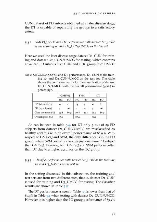
5.3.2 GMLVQ, SVM and DT performance withdataset D1_CUN as the training set andD2_CUN/UMCG as the test set 73

5.3.3 Classifier performance with dataset D1_CUNas the training set and D3_UMCG as thetest set 73

5.3.4 Classifier performance with dataset D3_UMCGas the training set and D1_CUN as thetest set 74

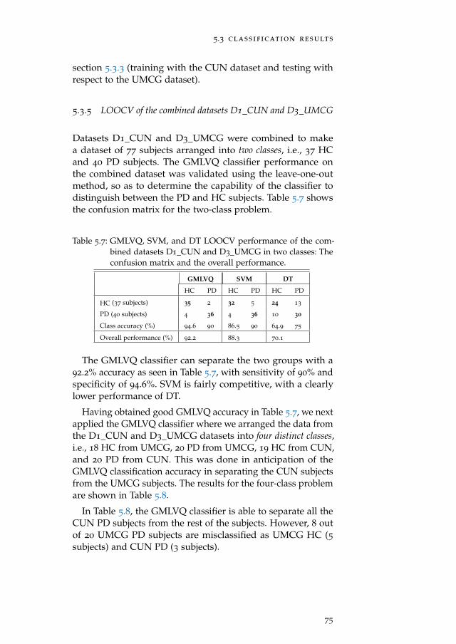
5.3.5 LOOCV of the combined datasets D1_CUNand D3_UMCG 75

5.4 Discussion and Conclusion 76

viii

contents

6 summary and conclusions 79

6.1 Summary and Discussion 79

6.2 Future Work 81

publications 95

samenvatting 97

acknowledgements 101

curriculum vitae 103

ix

1I N T R O D U C T I O N

T he diagnosis of neuro-degenerative diseases characterisedby slow progression is difficult, especially at an earlystage. These diseases have continued to affect the el-

derly [Berg, 2008], especially in developed countries where lifeexpectancy is high. Some of these disorders include Parkin-son’s disease (PD), progressive supranuclear palsy (PSP), multi-system atrophy (MSA), Alzheimer’s disease (AD), frontotem-poral dementia (FTD), and dementia with Lewy bodies (DLB),to mention a few. Parkinson’s disease (PD) is a progressive dis-order which causes slow motion and rigidity in the body. PD ischaracterized by neuronal loss in the substantia nigra and otherbrain regions, also associated with the formation of intracel-lular protein inclusions known as Lewy bodies [Shulman andDe Jager, 2009]. On the other hand, Alzheimer’s disease (AD)is associated with progressive memory loss, as well as judg-ment and decision making impairments, according to statisticscollected by Guttmacher et al. [2003].

There is increasing interest to use neuroimaging techniquesin the hope to discover biomarkers, that is, abnormal patternsof morphology, energy consumption or network activity ofthe brain which are characteristic for such diseases. Many invivo brain imaging techniques are nowadays available for thispurpose; see Table 1.1. Positron Emission Tomography (PET)has been applied in many medical studies due to its capa-bility to show metabolism of the brain. PET scans reveal theamount of metabolic activity in various parts of the brain. PETis used for clinical diagnosis of brain diseases. For example,in patients with idiopathic Parkinson’s disease (IPD), a pat-tern of increased metabolism in specific brain areas was foundon the basis of Positron Emission Tomography (PET) imaging[Fodero-Tavoletti et al., 2009]. This method is based on visualcomparison of patient data with disease-specific templates thatcontain regions of interest (ROIs), and is therefore quite sub-jective. Other studies to detect and differentiate parkinsoniansyndromes include Eckert et al. [2005, 2008]; Hellwig et al.[2012]; Wu et al. [2013]; Garraux et al. [2013]. On the other

1

introduction

hand, PET has been used in previous studies to test for depres-sion and dementia in patients with neurodegenerative diseases.For example, as reported by Chow et al. [2009], PET was usedto measure the availability of cortical serotonin receptors inolder subjects. PET can also be used to perform efficient di-agnosis [Yun et al., 2001]. Newly developed PET techniquesuse multivariate statistical analysis to identify disease-relatednetwork patterns of brain metabolism [Frackowiak et al., 2003].

Although this thesis focuses on PET for image acquisition,we briefly mention some other methods, also because someof these may be combined with PET in future work. A largecollection of brain imaging techniques is based upon MagneticResonance Imaging (MRI) [Golder, 2002]. In contrast to PET,which requires administering radioactive tracers to the subjectbeing scanned, MRI is a fully non-invasive method with noknown health implications. In fact, distinct spatial patterns ofcortical atrophy have been found from structural MRI imagesby a technique called voxel-based morphometry (VBM) [Chéte-lat et al., 2008; Berg, 2008]. This method considers all voxels in abrain volume, and gives quantitative estimates of the grey andwhite matter volumes without assuming any a priori regions ofinterest. Another MRI-based technique, called Diffusion TensorImaging (DTI), is able to measure the amount of anisotropyof water diffusion, from which the orientation of nerve fiberbundles in brain white matter can be inferred [Basser et al.,1994]. Also, in the study by Ito et al. [2006] measures like ap-parent diffusion coefficient (ADC) and fractional anisotropy(FA) have been used to evaluate the degree of tissue degenera-tion in diseases like Parkinson’s and multiple system atrophy.In addition, DTI-tractography can be used to visualise nervefiber tracts and study abnormal connectivity patterns betweenbrain regions. Furthermore, MRI-based techniques such as Arte-rial Spin Labelling (ASL) and Susceptibility-Weighted Imaging(SWI) allow for quantitative assessment of tissue perfusion andlevels of venous blood, hemorrhage, and iron storage in thebrain, respectively. Additionally, the MRI-technique known asfunctional magnetic resonance imaging (fMRI) determines andvisualises changes in brain activity that are elicited by askingtest persons to carry out specific cognitive or sensorimotor tasks.A recent addition is “resting-state” fMRI, where the subject inthe MRI-scanner is imaged without external stimulus; the dataare processed to derive brain connectivity patterns which areassumed to represent a default-mode network [Salvador et al.,

2

introduction

2005] and other networks mentioned by Van Den Heuvel andPol [2010]. This network includes regions that are known to beimpaired in certain types of neuro-degenerative diseases [Gre-icius, 2008]. For completeness, we also have listed some imagingtechniques in Table 1.1 which can detect neuronal activity, likeelectroencephalography (EEG) and magnetoencephalography(MEG).

Table 1.1: In vivo brain imaging techniques. See Figure 1.1 for a PETbrain image example.

Technique Represents Physical effect

CT anatomy X-ray attenuation

PET metabolism radioactive decay

MRI anatomy magnetic resonance

fMRI metabolism blood deoxygenation

DTI nerve fibers anisotropic diffusion

MEG neuronal activity magnetic signals

EEG neuronal activity electric signals

Figure 1.1: In vivo brain imaging techniques: example of a PET brainimage.

Although some success has been obtained by the techniquesmentioned above, a major problem is that each of the separatebrain imaging modalities only produces a clearly observabledisease-related brain pattern when the disease has reached anadvanced stage. Also, abnormal patterns may not be specificfor a single brain disease. Functional imaging methods (PET,fMRI) may give only a partial picture due to compensatorymechanisms in patients with neuro-degenerative diseases. It

3

introduction

is increasingly recognised that combining information derivedfrom different image modalities is essential for improvementof the sensitivity and specificity of proposed biomarkers forneuro-degenerative diseases [Davatzikos et al., 2008]. Anothershortcoming of current efforts is that only very few studies inthe literature report abnormal patterns for a given disease, sothat reproducibility of these findings is not yet firmly estab-lished. Also, the typical size (10-20) of patient groups is toosmall to differentiate between subtypes of a given disease (suchas akinetic-rigid versus tremor-dominant PD). It is clear thatprogress in the early diagnosis of neuro-degenerative diseasescan only be made if both imaging and diagnostic data of largenumbers of patients in several phases of disease progressionare accumulated. Also, for the many MRI-based techniquesfurther improvements may be possible by optimising scannersequences for each modality, which therefore have to be care-fully recorded for each scan session. This will require substan-tial efforts in database formation during longitudinal studiesspanning several decades.

1.1 objective

The objective of this thesis is, first, to derive features from med-ical imaging data in the hope to discover more sensitive andspecific biomarkers for the prediction of neuro-degenerativediseases. Second, to develop supervised classification methodsfor associating brain patterns (and features) extracted frommulti-modal brain imaging data to various types and stages ofneuro-degenerative diseases.

1.1.1 Specific Objectives

• To collect medical data and use it to identify structuraland functional brain patterns that display significantdifferences between healthy subjects and patients withneuro-degenerative diseases.

• To develop classification methods based on the brainfeatures extracted from the multi-modal brain images.

• To test the performance of the developed methods.

4

1.2 techniques and tools


1.2.1 Imaging Data Acquisition by Positron Emission Tomography

In this thesis PET was used for image acquisition. PET is animaging technique that uses radioactive material to diagnosediseases. The radiotracer is injected into a patient, where itaccumulates in the body to the specific part of interest. Thetracer emits positrons which are annihilated by electrons underemission of gamma rays. The gamma rays are detected by adevice called a gamma camera. The device works with the com-puter to measure the position-dependent amount of radiotracerabsorbed by the body, thus producing a brain image.

limitations of pet

• The scan session takes quite a long time (approximately30 to 40 minutes [Carne et al., 2007]) in addition to timereserved for the radiotracer (45 to 60 minutes [Townsend,2004]) to accumulate in the body part of interest. Theduration of the whole scan process also depends on thetissue under observation.

• The PET scan may show false results in case of chemicalimbalances in the body.

1.2.2 Analysis Tools

A number of analysis tools are briefly mentioned here forcompleteness because they are used to pre-process the PETbrain images [Teune et al., 2013], but are not further discussedin this thesis.

1.2.2.1 Statistical Parametric Mapping (SPM)

The SPM package [Friston et al., 2007] can be used to processimages for feature extraction. Processing of images can includesegmentation, co-registration and normalisation, all which arefound in the SPM package.

5

introduction

1.2.2.2 Voxel Based Morphometry (VBM)

VBM is a very useful method to analyse images on the voxellevel Ashburner and Friston [2000]. For example, in the studyby Chételat et al. [2008], VBM was used to determine the differ-ence in levels or stages of progression of NDs like Alzheimer’s.VBM has also been used to differentiate several NDs based onpathology. Burton et al. [2004] used VBM to study the patternof cerebral atrophy in PD in comparison to healthy controls,AD and DLB; the result was that atrophy is greater in somebrain areas for AD than for PD. Generally VBM has been usedfor differentiation of several NDs and their stages.

1.2.3 Classification Tools/Pattern classification

Supervised classification methods for associating brain patternsto various forms of neuro-degenerative disease will be appliedto PET data in this thesis. By using a data set of subjects whosediagnosis has been determined by medical experts, a classifieris trained using the set of features in conjunction with subjectlabels. After training, the classifier can be used to classify newsubjects for which their diagnosis is unknown. Extracted fea-tures of the new subject are compared with the training setfeatures indirectly. That is to say, using the rules establishedby the classifier during the training, the classifier computes thebest matching disease type(s). This procedure is visualised inFigure 1.2. The training phase of the classification system isshown on the left. The classification or query phase, shownon the right, employs the same procedures, the features areextracted from the test case(s) and used for classification. Thatis, the label(s) of the test/query image(s) is determined.

An important requirement for this method to work is that thenumber of training samples per disease (sub)type is sufficientlyhigh. As more training data become available in the courseof time the classifiers are expected to increase in classificationperformance.

There are many different classification methods in neural-network and statistical-decision theory. Within learning andreasoning approaches, decision trees (DT) are among the mostpopular ones [Breiman et al., 1984; Quinlan, 1993]. They are alsointuitive for non-experts, since the DT procedure correspondsto the way humans perform classification based on many fea-

6


Figure 1.2: Classification System: On the left is the training phase andon the right is the testing phase.

tures (like in taxonomy). Therefore we start our investigationswith this classification method. After DT, we concentrate onlinear classifiers (with linear decision boundary) because morecomplex systems (multilayered neural networks, SVM withnon-linear kernel etc.) might be at risk to over-fit the relativelysmall datasets. Distance based methods such as GeneralizedMatrix Learning Vector Quantization (GMLVQ) will be appliedand compared with the decision tree algorithms. Feature reduc-tion/definition is an integral part of these methods [Schneideret al., 2007]. Alternative classifiers such as the Support VectorMachine (SVM) [Hammer et al., 2004] will be applied as well.

1.2.3.1 Decision trees

A decision tree represents a recursive partition of the instancespace [Rokach and Maimon, 2010]. It consists of at least a rootnode which can be connected by successive edges to childnodes. These child nodes, also known as internal nodes, are inturn connected to child nodes, until the leaf nodes are reachedwhich do not have out-going edges. A new data example isclassified by going through a path from the root node to the leafnode, while testing each feature of that example represented ateach of the internal nodes. Based on the outcome of each test,a sequence of edges is followed until a leaf node is reached.

7

introduction

Since each leaf carries a class label, the new data example isassigned the class of the leaf it reaches. There are algorithmsthat can be used to construct decision trees which includeC4.5 [Quinlan, 1993], CART Breiman et al. [1984] and others. Inparticular, the C4.5 decision tree inducer uses an informationtheoretic criterion to build decision trees. A dataset is split intosubsets at each node by choosing the attribute/feature thatmaximizes the information gain. The details about informationgain are found in chapter 3. The optimal decision tree is theone which minimizes the generalization error. Increased robust-ness is provided by applying “bagging” [Breiman, 1996]. Forthe problem considered here, i.e., brain images which wouldrequire human interpretation, a decision tree-based approach isvery suitable, because it resembles the way that human expertsperform classification.

1.2.3.2 Generalized Matrix Learning Vector Quantization

GMLVQ estimates the relevance of features in their ability toclassify data. Then the classifier uses the weighted features(according to their relevance) and class prototypes to separategroups of data. This is possible with the full matrix Λ whichaccounts for pairwise correlations of the feature dimensions.A distance metric is used that has the form dΛ(wk,x) = (x−wk)

TΛ(x−wk), where Λ is a positive semi-definite N × Nmatrix which is used to quantify the dissimilarity of an inputvector x and the prototypes wk [Schneider et al., 2009].

1.2.3.3 Support Vector Machine

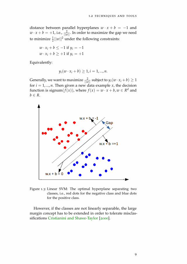
The Support vector machine determines the optimal hyper-plane with the largest distance or margin between supportvectors (border-line training data examples) separating the in-stances in the feature space. A new data example is classifiedas belonging to either of the classes separated by the hyper-plane. For example, given training data with input vectorsx1, x2, ..., xn ∈ Rd and labels y1, y2, ..., yn ∈ {−1,+1} [Oz andKaya, 2013], as shown in Figure 1.3, we need to find an optimalhyperplane w · x + b = 0 (i.e., vector w and the scalar b) whichseparates the negative data examples from the positive dataexamples. There could exist a number of such hyperplanes, butSVMs find the hyperplane that maximizes the gap betweenthe support vectors. This gap (as seen in Figure 1.3) is the

8


distance between parallel hyperplanes w · x + b = −1 andw · x + b = +1, i.e., 2

||w|| . In order to maximize the gap we need

to minimize 12 ||w||2 under the following constraints:

w · xi + b ≤ −1 if yi = −1

w · xi + b ≥ +1 if yi = +1

Equivalently:

yi(w · xi + b) ≥ 1, i = 1, ..., n.

Generally, we want to maximize 2||w|| subject to yi(w · xi + b) ≥ 1

for i = 1, ..., n. Then given a new data example x, the decisionfunction is signum( f (x)), where f (x) = w · x + b, w ∈ Rd andb ∈ R.

Figure 1.3: Linear SVM: The optimal hyperplane separating twoclasses, i.e., red dots for the negative class and blue dotsfor the positive class.

However, if the classes are not linearly separable, the largemargin concept has to be extended in order to tolerate misclas-sifications Cristianini and Shawe-Taylor [2000].

9

introduction

1.2.4 Visualization Tools

In addition to the pattern recognition algorithms, we willalso apply visualisation techniques such as scatter plot ma-trices [Zheng et al., 2014], decision tree diagrams [Stiglic et al.,2012], or multiple views [Wang Baldonado et al., 2000] to ex-plore the labeled data sets in feature space. Visualisation meth-ods will serve two important goals. First, they will give aninsight in the distribution of the data points in the featurespace, hence portraying an idea of how data can be separatedinto distinct classes. Second, visualisation allows an intuitiveway to present the results to the medical experts, thereby facili-tating communication.

1.3 ssm/pca method for feature extraction

The scaled subprofile model with principal component analysis(SSM/PCA) [Moeller et al., 1987; Moeller and Strother, 1991]is used in this thesis to extract patterns from PET data withthe removal of the group mean and the voxel mean, therebyremoving the overall major subject and group global effects be-fore applying PCA to the data. This process makes evident themain patterns of metabolic brain activity in the data. It is fromthese patterns that the features to be used in the classificationprocess are determined.

In this thesis, the extracted features depend entirely on thewhole input dataset, since they are produced by PCA. Thismakes the leave-one-out method used for performance evalu-ation more complicated than usual. In other words, since thefeatures are dependent on the input data, for each leave-one-out run, a test subject is always removed from the trainingset before applying the SSM/PCA method and later projectedonto the extracted patterns (from the training set) to obtain itsscores.

1.4 thesis contribution and content

Machine learning methods are employed in the classificationof neurodegenerative diseases. In chapter 2, which is basedon [Mudali et al., 2015], we look at the classification of parkin-sonian syndromes since they are not easily separable. We used

10

1.4 thesis contribution and content

the C4.5 decision tree inducer [Quinlan, 1993] to train classifierson the subject scores as features extracted from FDG-PET data.

Having applied a different method called stepwise regression(SR) [Teune et al., 2013] to the same parkinsonian syndromesdata, we studied the difference between this method and thedecision tree (DT) method. This is the topic of chapter 3, whichis based on [Mudali et al., 2016c].

Other classification methods were introduced in chapter 4

in the hope to improve classification accuracy. This chapteris based on [Mudali et al., 2016b]. The GMLVQ and SVMclassifiers were trained using features extracted from the FDG-PET data, similar to the method used in chapter 2 and chapter 3.The same SSM/PCA method was applied to the FDG-PETdata to extract the features, specifically subject scores. Thesesubject scores were input to the GMLVQ and SVM classifiersto determine the correct subject(s) label(s). Using leave-one-outcross validation, the classifier performances were evaluated.

In chapter 5, which is based on [Mudali et al., 2016a], morePD data consisting of later disease stage brain images was ac-quired and combined with the early stage data. The three clas-sification methods i.e., decision trees, GMLVQ and SVM, wereapplied to combinations of the early and late-stage datasets.Additionally, we interchanged the later and earlier disease stagedatasets for training and testing the classifiers.

Lastly, chapter 6 contains a summary of the thesis and possi-bilities for future work.

11

2C L A S S I F I C AT I O N O F PA R K I N S O N I A NS Y N D R O M E S F R O M F D G - P E T B R A I N D ATAU S I N G D E C I S I O N T R E E S W I T H S S M / P C AF E AT U R E S

abstract: Medical imaging techniques like fluorodeoxyglucose positron emission

tomography (FDG-PET) have been used to aid in the differential diagnosis of neu-

rodegenerative brain diseases. Visual Interpretation of FDG-PET scans and clinical

symptoms of patients with neurodegenerative brain diseases can be difficult, especially

at an early disease stage. In this study, the objective is to classify FDG-PET brain

scans of subjects with parkinsonian syndromes (Parkinson’s disease, Multiple System

Atrophy, and Progressive Supranuclear Palsy), compared to healthy controls. The

scaled subprofile model/principal component analysis (SSM/PCA) method was applied

to FDG PET brain image data to obtain covariance patterns and corresponding subject

scores. The latter were used as features for supervised classification by the C4.5 decision

tree method. Leave-one-out cross validation was applied to determine classifier perfor-

mance. We carried out a comparison with other types of classifiers. The performance of

the decision tree method is in some cases (somewhat) lower than that of other classifiers

like nearest neighbors or support vector machines. However, the big advantage of

decision tree classification is that the results are easy to understand by humans. A

visual representation of decision trees strongly supports the interpretation process,

which is very important in the context of medical diagnosis. Further improvements are

suggested based on enlarging the number of the training data, enhancing the decision

tree method by bagging, and adding additional features based on (f)MRI data.

Keywords: Parkinsonian syndromes, FDG-PET data, scaled subprofile model,

principal component analysis, decision tree classification, visual analysis.

2.1 introduction

Neurodegenerative brain diseases like Parkinson’s disease (PD),multiple system atrophy (MSA), or progressive supranuclearpalsy (PSP), are difficult to diagnose at early disease stages[Litvan et al., 2003]. It is important to develop neuroimag-ing techniques that can differentiate among the various formsof parkinsonian syndromes and stages in progression. Earlydisease detection is aided by brain imaging techniques like[18F]-fluorodeoxyglucose (FDG) positron emission tomography

13

decision tree classification of parkinsonian syndromes

(PET) and magnetic resonance imaging (MRI), to obtain imagedata and derive significant patterns of changed brain activity.Several techniques have been developed to identify disease-related network patterns of cerebral glucose metabolism.

Covariance techniques like principal component analysis(PCA) can be used to extract significant patterns from brainimage data. PCA is known for its capability to identify patternsin high-dimensional data like brain image data. A possible ap-proach to biomarker identification is the scaled subprofile mod-el/principal component analysis (SSM/PCA) method [Moelleret al., 1987; Moeller and Strother, 1991]. SSM/PCA is a featureextraction method which enhances identification of significantpatterns in multivariate imaging data. This method has beenextensively applied to positron emission tomography data toidentify brain patterns which display significant differencesbetween healthy controls and parkinsonian conditions. TheSSM/PCA method helps to reduce data dimensions and to re-veal the brain patterns characteristic for a certain parkinsoniansyndrome. Resting state metabolic networks obtained fromFDG-PET scans were used to identify disease related metabolicbrain patterns of PD, MSA and PSP [Ma et al., 2007; Eckertet al., 2008; Eidelberg, 2009; Teune et al., 2013]. In a previousstudy by Tang et al. [2010], it was demonstrated that by usingan image-based classification routine, it was possible to distin-guish with high specificity between PD and MSA/PSP, and ina second step between MSA and PSP as compared to controls.

In a recent study of Hellwig et al. [2012], the diagnosticaccuracy of FDG-PET in discriminating parkinsonian patientswas investigated. FDG-PET scans were analyzed by visualassessment including individual voxel based statistical maps(a 3D stereotactic surface projection technique; 3D-SSP). Thesestudies compared only two classes at a time or on two levels(healthy and patient group, or two patient groups). This putsforward a research challenge to improve the SSM/PCA method,to be able to distinguish different neurodegenerative braindiseases from each other in one analysis.

For this reason we consider machine learning approacheslike decision-tree methods to be able to compare more than twopatient groups at the same time and possibly detect subtypeswithin patient groups. The C4.5 decision tree classificationalgorithm by Quinlan [1993] is used to classify parkinsonianconditions from FDG-PET imaging data. This algorithm uses a

14

2.2 materials and methods

feature selection criterion known as information gain to inducedecision trees from training data. The subject scores derivedfrom the SSM/PCA method are used as input features for theC4.5 algorithm. After the training phase, the decision treescan then be used as predictors for unseen cases with unknowndisease type. Decision trees are known to be intuitive and easilyunderstandable by humans [Cintra et al., 2012]. In other words,they can be easily visualized and interpreted by the clinicians.

In this chapter, we combine the SSM/PCA method in a novelway with the C4.5 decision tree classification algorithm whichclassifies parkinsonian disorders according to their respectivedisease types. We also compare the decision tree method witha number of other classifiers with respect to different criteria,such as performance and interpretability by humans.


The extraction of patterns and classification involves four mainsteps: data acquisition, feature extraction, feature selection, andclassification, see Figure 2.4.

Figure 2.4: Classification steps.

2.2.1 Data Acquisition

FDG-PET scans from a previous study [Teune et al., 2010]describing 18 healthy controls (HC), 20 PD, 21 MSA, and 17

PSP patients were used for the present analysis. At the time ofreferral for imaging, the clinical diagnosis of most patients wasuncertain. The final clinical diagnoses according to establishedclinical research criteria [Gilman et al., 2008; Litvan et al., 1996,2003] were made after a follow-up time after scanning of 4±3

15


years (y) in PD, 2±1y in MSA, and 3±2y in PSP. IncludedPD patients were 9 male (M), 11 female (F), 6 right body-sideaffected, 14 left-side affected, with mean age of 63±9y andDisease Duration (DD) at scanning of 3±2 years. Fourteenprobable MSA, 7 possible MSA patients (10M, 11F, age 64±10y;DD 4±2y), and 13 probable, 4 possible PSP patients (9M, 8F,age 68±8y; DD 2±1y) were included.

2.2.2 Feature Extraction

We reimplemented the SSM/PCA method in Matlab based onthe description by Spetsieris and Eidelberg [Eidelberg, 2009;Spetsieris et al., 2010; Spetsieris and Eidelberg, 2011; Spetsieriset al., 2009]. First, the FDG-PET images are loaded in a datamatrix Psv, and a mask is applied to each subject image inPsv (s [1,...,M] refers to subjects and the column index v refersto voxels) to remove all voxels with intensity value less than35% of the whole brain volume maximum. Then the subjectmatrix is log-transformed and doubly centered to create asubject residual profile (SRP) matrix SRPsv. PCA is then ap-plied to the matrix SRPsv to obtain its eigenvectors. Theseeigenvectors are called Group-Invariant Subprofile (GIS) pat-terns (GISk, k = 1, 2, ..., M), and represent characteristic disease-related brain patterns. Furthermore, subject scores are com-puted as the contribution of each subject image to a diseaserelated pattern GISk.

Figure 2.5 illustrates the flow of the program. The main stepsof the method are as follows, see [Spetsieris and Eidelberg,2011].

1. The FDG-PET images are loaded into a data matrix Psv1

of dimension M × N, where the row index s (1,...,M)refers to subjects, and the column index v refers to vox-els. So row s contains the 3D image data for subject s,reformatted in vector form.

2. A mask is applied to each subject image in Psv to reducelow values and noise in the brain volumes. In this study,all voxels with intensity value less than 35% of the wholebrain volume maximum were removed to create individ-ual masks. Next a group mask with non-zero values for

1 By expressions like “the matrix Psv” we mean the matrix P with elements Psv.

16


Figure 2.5: Computation flow chart illustrating SSM/PCA analysis.For explanation see text.

all subjects is created by taking the intersection of theindividual masks.

3. The subject matrix Psv is log-transformed to obtain thematrix LogPsv. This step is necessary in order to removemultiplicative scaling effects.

4. The log-transformed subject matrix is doubly centered.The mean across voxels (local glucose metabolic rateLGMR) for each subject and the mean across subjects(GMP image) is subtracted from the matrix LogPsv tocreate a subject residual profile matrix SRPsv, i.e.,

SRPsv = LogPsv − LGMRs −GMPv

where

LGMRs = meanvox(LogPsv)

GMPv = meansub(LogPsv)−meansub(LGMRs)

Here meanvox is the mean across voxels per subject andmeansub is the mean across subjects per voxel. This dou-ble centering is carried out in order to: 1) remove offsetdifferences per subject 2) remove offsets per voxel, i.e.,enhance/retain differences between subjects per voxel;removing uninformative overall behaviour.

5. PCA is applied to the matrix SRPsv. The eigenvectorsof the PCA analysis are called Group-Invariant Subpro-file (GIS) patterns (GISk, k = 1, 2, ..., M), and representcharacteristic brain patterns.

17


6. Subject scores are computed as the amount of expressionof a subject on a disease related pattern GISk. The scoreof subject s for the kth GIS pattern is defined as the innerdot product of the subject’s SRP row vector and the kthGIS vector:

Scoreks = SRPTs ·GISk (2.1)

The SSM/PCA method was applied to several data groups(disease group(s) compared to healthy controls) in trainingset(s) from which disease related patterns (GISk) were extractedwith positive and negative loadings (voxel weights) [Ma et al.,2009]. The brain images from the training set are weighted ontothe patterns to obtain subject scores, which depict how mucheach subject image contributes to a pattern.

Subject scores as features for classification

Features are usually derived as characteristics of an object suchas texture, color, or shape [Westenberg and Roerdink, 2002],which can be computed for each subject (data set) separately.The use of PCA-based subject scores as features deviates sig-nificantly from the standard situation through the fact thatfeatures now depend on the whole dataset. Also, the numberof features is, at least initially, equal to the number of principalcomponents which is equal to the number of data sets. So whena subject is removed or added to the data collection the scoresof all the other subjects change as well. Therefore, there is needto redo the SSM/PCA procedure once the dataset changes toobtain new scores.

2.2.3 Decision tree classification

The C4.5 decision tree method [Quinlan, 1996b] is a supervisedlearning strategy which builds a classifier from a set of trainingsamples with a list of features (or attributes) and a class label.The algorithm splits a set of training samples into subsets suchthat the data in each of the descending subsets are “purer” thanthe data in the parent subset (based on the concept of informa-tion gain from information theory). Each split is based on anoptimal threshold value of a single feature. The result is a treein which each leaf carries a class name and each interior nodespecifies a test on a particular feature. The tree constructed in

18


the training phase of a decision tree classifier can be drawn inan easy to understand graphical representation which showsthe successive features and threshold values which the algo-rithm has used to separate the data set in non-overlappingclasses. Once a tree has been obtained from the training sam-ples, it can be used for testing to classify unseen cases wherethe class label is unknown.

The C4.5 decision tree algorithm [Quinlan, 1993] has beenused in many previous studies, ranging from diatom identifi-cation [du Buf and Bayer, 2002] to classification of anomalousand normal activities in a computer network to curb intru-sions [Muniyandi et al., 2012]. The method has also been ap-plied to improve accuracy in multi-class classification problems.For example, Polat and Günes [2009] applied a novel hybridclassification system based on the C4.5 decision tree classifierand a one-against-all approach, obtaining promising results.In addition, Ture et al. [2009] analysed several decision treemethods (CHAID, CART, QUEST, C4.5, and ID3) together withKaplan-Meier estimates to investigate their predictive powerof recurrence-free survival in breast cancer patients, they re-port that C4.5 performed slightly better than other methods.In summary, decision trees are considered to be powerful forclassification and are easy to interpret by humans. Not only arethey simple and effective, but they also work well with largedatasets [Perner, 2001].

decision tree classification of parkinsonian syn-dromes Using the C4.5 machine learning algorithm, wetrained classifiers on subject scores of extracted patterns forhealthy subjects and subjects with known types of neuro-degenerative disease. The result is a pruned decision tree show-ing classified subject images. The goal of pruning is to obtain atree that does not overfit cases. Note that it would be possibleto obtain 100% correct classification in the training phase byusing a less stringent pruning strategy. However, this wouldcome at the expense of generalization power on unseen cases.

In contrast to applications of the SSM/PCA method whichmake a pre-selection of principal components (GIS vectors)on which the classification will be based, the C4.5 algorithmuses all principal components and the corresponding subjectscores as input. The algorithm itself determines which principalcomponents are most discriminative to separate the data set

19


into classes. More discriminative components appear higherin the decision tree, i.e., closer to the root; refer to Figure 2.6for an example, where the subject score SSPC5 is the mostdiscriminative feature.

In order to apply the C4.5 classifier to unseen cases, the re-quired subject scores for testing are first computed by projectingthe SRP of the new subject on the GIS profiles of the trainingset according to Eq. (2.1). The computation of the SRP for theunseen case involves centering along the subject dimension, i.e.,subtracting the GMP (group mean profile). The assumption isthat this GMP can be obtained from the reference group only,i.e., the group used for training the classifier; see the discussionin Spetsieris et al. [2009], [p. 1244].

2.2.4 Other Classifiers

We also applied a number of other classifiers: nearest neighbors;linear classifiers: linear discriminant analysis and support vec-tor machines; random forests, which is an extension of decisiontrees; classification and regression trees (CART) for predictingreal/continuous variables; and naive Bayes, a probabilistic clas-sifier. Linear classifiers in particular are simple to implement.They are known to work better in situations where the data isuniformly distributed with equal covariance.

nearest neighbors (nn) NN is a classification methodwhich assigns a class to a new data point based on the classof the nearest training data point(s). In the K-NN (K-NearestNeighbors) method, distances to the neighbors are computedfirst. Then, a new data point receives the majority label of theK nearest data points.

linear discriminant analysis (lda) LDA, like PCA,is used for data classification and dimensionality reduction.This classifier maximizes the between-class variance and mini-mizes the within-class variance to ensure a clear separation indatasets. Accordingly, the training data are first transformed,then the data in the transformed space are classified as belong-ing to a class which minimizes the Euclidean distance of itsmean to the transformed data [Fukunaga, 1990].

20

2.3 results and discussion

support vector machine (svm) SVM performs classifi-cation by generating an optimal decision boundary in the formof a hyperplane which separates different classes of data pointsin the feature space. The decision boundary should maximizethe distance between the hyperplane and support vectors calledthe margin [Duda et al., 2000].

random forests Random Forests is a machine learningmethod for classification of objects based on a majority vote ofa multitude of decision trees. This method combines bagging(random selection of cases) and random selection of features(at each node) during the training phase. Also, the trees are notpruned.

classification and regression trees (cart) CART,just like C4.5, is a decision tree learning method. However, inaddition to using decision trees as predictors, CART includesregression trees for predicting continuous variables.

naive bayes This is a method that classifies data pointsbased on their likelihood and the prior probabilities of occur-rences of known classes. The final classification is achievedby combining the prior and the likelihood to form a posteriorprobability using Bayes’ rule. Overall, the new data will belongto a class which maximizes the posterior probability.


2.3.1 Results for decision tree classifiers

Decision tree classifiers were trained by applying the C4.5algorithm to individual (each disease group versus healthycontrols) and combined datasets of PD, PSP, MSA patientsand healthy controls (HC) with known class labels, as listed inSection 2.2.1. For the individual datasets, we were interestedin identifying features which best separate two groups (i.e., adisease group from healthy controls). For the combined datasetswe compared all the groups, that is, PD, MSA, PSP, and HCto each other to obtain feature(s) which can separate the fourgroups. Tree pruning was carried out by using the defaultvalues of the C4.5 algorithm [Quinlan, 1993].

21


2.3.1.1 Building classifiers for individual datasets

Decision tree classifiers were built in the training phase fromthe individual datasets (PD, PSP, MSA) compared to the HCgroup of 18 subjects.

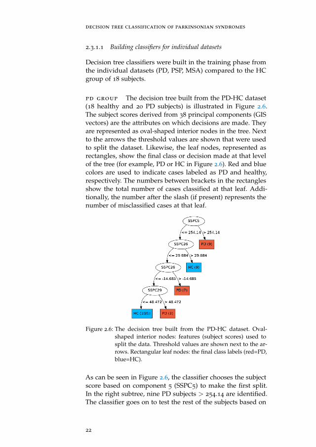
pd group The decision tree built from the PD-HC dataset(18 healthy and 20 PD subjects) is illustrated in Figure 2.6.The subject scores derived from 38 principal components (GISvectors) are the attributes on which decisions are made. Theyare represented as oval-shaped interior nodes in the tree. Nextto the arrows the threshold values are shown that were usedto split the dataset. Likewise, the leaf nodes, represented asrectangles, show the final class or decision made at that levelof the tree (for example, PD or HC in Figure 2.6). Red and bluecolors are used to indicate cases labeled as PD and healthy,respectively. The numbers between brackets in the rectanglesshow the total number of cases classified at that leaf. Addi-tionally, the number after the slash (if present) represents thenumber of misclassified cases at that leaf.

Figure 2.6: The decision tree built from the PD-HC dataset. Oval-shaped interior nodes: features (subject scores) used tosplit the data. Threshold values are shown next to the ar-rows. Rectangular leaf nodes: the final class labels (red=PD,blue=HC).

As can be seen in Figure 2.6, the classifier chooses the subjectscore based on component 5 (SSPC5) to make the first split.In the right subtree, nine PD subjects > 254.14 are identified.The classifier goes on to test the rest of the subjects based on

22


Figure 2.7: The decision trees built from the MSA-HC (left) and PSP-HC (right) datasets. For details, refer to Fig. 2.6.

component 26, where nine subjects (subject score > 29.684) areidentified as HC; etc. Only one PD subject is misclassified asHC, as can be seen in Figure 2.6 in the lower-left rectangle.

msa group The decision tree built from the MSA-HC dataset(18 healthy and 21 MSA subjects) is illustrated in Figure 2.7(left). The attributes are subject scores derived from 39 principalcomponents. Again, one HC subject is misclassified

psp group The decision tree built from the PSP-HC dataset(18 healthy and 17 PSP subjects) is illustrated in Figure 2.7(right). The attributes are subject scores derived from 35 princi-pal components.

2.3.1.2 Building classifiers on combined datasets

We also applied the C4.5 classification algorithm to the com-bined datasets consisting of all four groups. Therefore, thedataset consisted of 76 subjects, 18 HC, 20 PD, 21 MSA and 17

PSP. Subject scores were obtained by applying the SSM/PCAmethod to the combined group. The resulting decision treeis shown in Figure 2.8. Three PSP subjects are classified erro-neously, two as PD and one as MSA.

23


Figure 2.8: The decision tree built from the combined PD-PSP-MSA-HC dataset.

2.3.1.3 Leave-one-out cross validation

In leave-one-out cross-validation (LOOCV), a single observationfrom the original dataset is used as the validation set (alsoknown as test set) and the remaining observations form thetraining set. This procedure is repeated N times where eachobservation is used once as a validation set.

The LOOCV method was applied to individual and com-bined datasets, i.e., PD-HC, MSA-HC, PSP-HC, and the com-bined dataset PD-MSA-PSP-HC to estimate classifier perfor-mance on unseen cases. Here performance is defined as thepercentage of correct classifications over the N repetitions. Toensure that attributes of the training set, and thus the trainedclassifier, are independent of the validation sample, the testsubject was removed from the initial dataset before applyingthe SSM/PCA method to the training set (with N − 1 samples)for obtaining the subject scores needed to train the C4.5 deci-sion tree classifier. The classifier was then used to determinethe label for the test subject. This procedure was applied foreach of the N subjects in the original dataset. Table 2.1 showsthe classifier performance.

As seen in Table 2.1, the C4.5 classifier performs highest withthe PSP group at 80% and lowest with the PD group at 47.4%.The feature at the root of a decision tree is most significantin classification, since it has the highest information gain (see

24


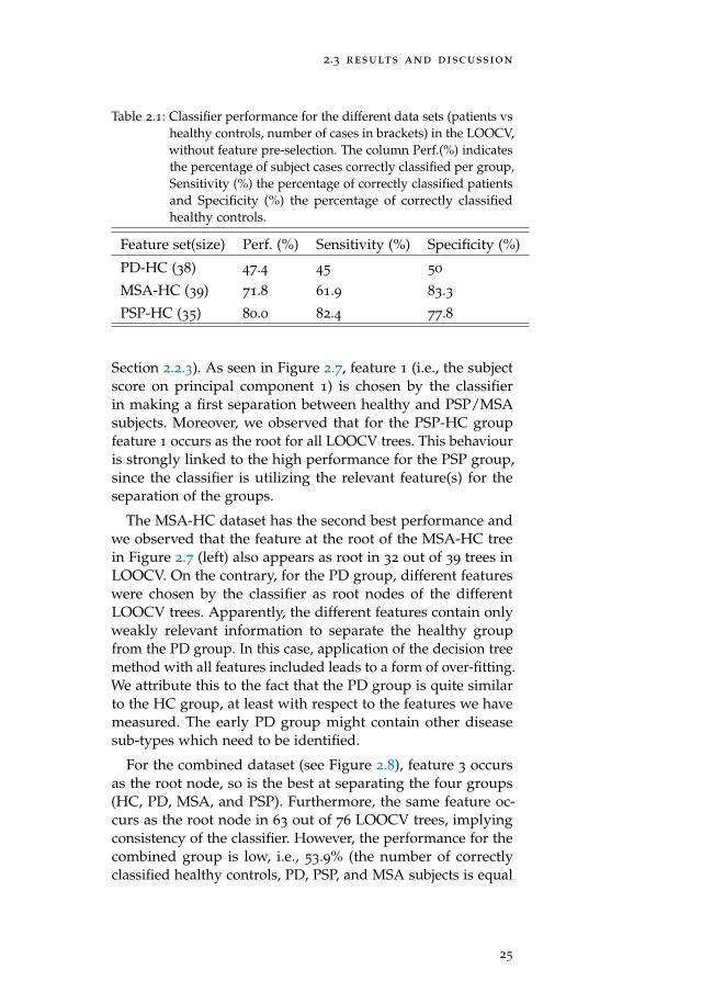
Table 2.1: Classifier performance for the different data sets (patients vshealthy controls, number of cases in brackets) in the LOOCV,without feature pre-selection. The column Perf.(%) indicatesthe percentage of subject cases correctly classified per group,Sensitivity (%) the percentage of correctly classified patientsand Specificity (%) the percentage of correctly classifiedhealthy controls.

Feature set(size) Perf. (%) Sensitivity (%) Specificity (%)

PD-HC (38) 47.4 45 50

MSA-HC (39) 71.8 61.9 83.3

PSP-HC (35) 80.0 82.4 77.8

Section 2.2.3). As seen in Figure 2.7, feature 1 (i.e., the subjectscore on principal component 1) is chosen by the classifierin making a first separation between healthy and PSP/MSAsubjects. Moreover, we observed that for the PSP-HC groupfeature 1 occurs as the root for all LOOCV trees. This behaviouris strongly linked to the high performance for the PSP group,since the classifier is utilizing the relevant feature(s) for theseparation of the groups.

The MSA-HC dataset has the second best performance andwe observed that the feature at the root of the MSA-HC treein Figure 2.7 (left) also appears as root in 32 out of 39 trees inLOOCV. On the contrary, for the PD group, different featureswere chosen by the classifier as root nodes of the differentLOOCV trees. Apparently, the different features contain onlyweakly relevant information to separate the healthy groupfrom the PD group. In this case, application of the decision treemethod with all features included leads to a form of over-fitting.We attribute this to the fact that the PD group is quite similarto the HC group, at least with respect to the features we havemeasured. The early PD group might contain other diseasesub-types which need to be identified.

For the combined dataset (see Figure 2.8), feature 3 occursas the root node, so is the best at separating the four groups(HC, PD, MSA, and PSP). Furthermore, the same feature oc-curs as the root node in 63 out of 76 LOOCV trees, implyingconsistency of the classifier. However, the performance for thecombined group is low, i.e., 53.9% (the number of correctlyclassified healthy controls, PD, PSP, and MSA subjects is equal

25


to 55.6%, 35%, 58.5%, and 66.7%, respectively). Our explana-tion is that the number of subjects per class is quite low giventhe large variability in each group. In addition, the combinedgroup is not well balanced in view of a relatively small size ofthe healthy subject group versus the combination of the threedisease groups.

permutation test In order to determine the significanceof the performance results we ran a permutation test on thePD-HC, MSA-HC, and PSP-HC groups [Al-Rawi and Cunha,2012; Golland and Fischl, 2003]. The steps of the procedure are:

1. for each group, perform a LOOCV on the original subjectlabels to obtain a performance PO;

2. repeatedly permute the labels and then do a LOOCVto obtain performances Pi for i = 1, . . . , Nperm (we usedNperm = 100)

3. compute the p-value as the total number of all Pi greateror equal to PO, divided by Nperm.

If p < 0.05 the original LOOCV result is considered to bestatistically significant.

The results of the permutation test were as follows. For thePSP-HC group: p = 0.00; for the MSA-HC group: p = 0.01;for the PD-HC group: p = 0.62. So we can conclude that forthe PSP-HC and MSA-HC groups the performance results aresignificant. However, for the PD-HC group this is not the case.This is consistent with the lack of robustness of the LOOCVtrees we already noted above. The healthy and PD group arevery similar and hard to separate, given the small number ofdatasets.

2.3.1.4 Pre-selection of features

In the hope to improve the classifier performance, we varied thenumber of features used to build the classifier in the LOOCV.This was done in two different ways: (i) by choosing the sub-ject scores of the n best principal components according tothe Akaike Information Criterion (AIC) [Akaike, 1974]; (ii) bychoosing the first n principal components arranged in orderof highest to lowest amount of variance accounted for. Theclassifier performance at the varying numbers of features isshown in Table 2.2.

26


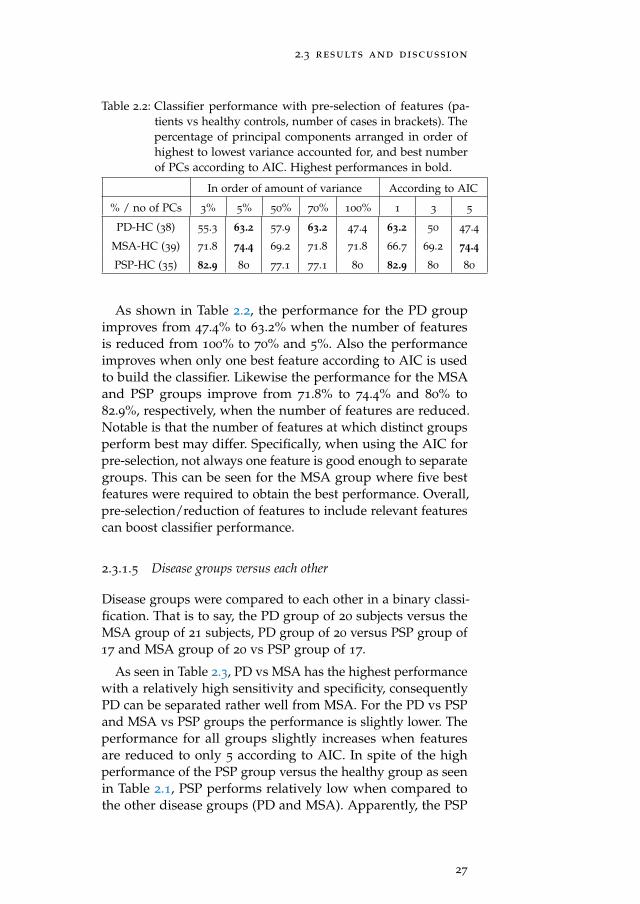
Table 2.2: Classifier performance with pre-selection of features (pa-tients vs healthy controls, number of cases in brackets). Thepercentage of principal components arranged in order ofhighest to lowest variance accounted for, and best numberof PCs according to AIC. Highest performances in bold.

In order of amount of variance According to AIC

% / no of PCs 3% 5% 50% 70% 100% 1 3 5

PD-HC (38) 55.3 63.2 57.9 63.2 47.4 63.2 50 47.4

MSA-HC (39) 71.8 74.4 69.2 71.8 71.8 66.7 69.2 74.4

PSP-HC (35) 82.9 80 77.1 77.1 80 82.9 80 80

As shown in Table 2.2, the performance for the PD groupimproves from 47.4% to 63.2% when the number of featuresis reduced from 100% to 70% and 5%. Also the performanceimproves when only one best feature according to AIC is usedto build the classifier. Likewise the performance for the MSAand PSP groups improve from 71.8% to 74.4% and 80% to82.9%, respectively, when the number of features are reduced.Notable is that the number of features at which distinct groupsperform best may differ. Specifically, when using the AIC forpre-selection, not always one feature is good enough to separategroups. This can be seen for the MSA group where five bestfeatures were required to obtain the best performance. Overall,pre-selection/reduction of features to include relevant featurescan boost classifier performance.

2.3.1.5 Disease groups versus each other

Disease groups were compared to each other in a binary classi-fication. That is to say, the PD group of 20 subjects versus theMSA group of 21 subjects, PD group of 20 versus PSP group of17 and MSA group of 20 vs PSP group of 17.

As seen in Table 2.3, PD vs MSA has the highest performancewith a relatively high sensitivity and specificity, consequentlyPD can be separated rather well from MSA. For the PD vs PSPand MSA vs PSP groups the performance is slightly lower. Theperformance for all groups slightly increases when featuresare reduced to only 5 according to AIC. In spite of the highperformance of the PSP group versus the healthy group as seenin Table 2.1, PSP performs relatively low when compared tothe other disease groups (PD and MSA). Apparently, the PSP

27


Table 2.3: Performance for binary classification of disease groups inthe LOOCV. The number of cases per group are in brackets.The column Perf. indicates the percentage of subject casescorrectly classified (all features included), Sensitivity thepercentage of correctly classified first disease group, Speci-ficity the percentage of correctly classified second diseasegroup, and Perf. (AIC-5) the performance when features arereduced to the best 5 PCs according to AIC.

Group Perf. (%) Sensitivity Specificity Perf. (AIC-5) (%)

PD vs MSA (41) 73.2 70 76.2 78

PD vs PSP (37) 67.6 80 52.9 70.3

MSA vs PSP (38) 68.4 76.2 58.8 71.1

features look more like those of PD or MSA patients than thoseof healthy controls.

2.3.1.6 Combined disease groups

Our main interest is to distinguish the Parkinsonian syndromesfrom each other. Therefore, we combined all disease groups(i.e., PD, PSP, and MSA) without the healthy controls in a de-cision tree multi-classification and applied LOOCV (at 100%features used). The performance of the classifier is 65.5%, with75% correctly classified PD subjects, 47.1% correctly classifiedPSP subjects, and 71.4% correctly classified MSA subjects. Al-together the PSP group has the lowest number of correctlyclassified subjects, in agreement with the previous observationthat it contains similarities to PD and MSA. Figure 2.9 showsthe decision tree diagram obtained after training the classifierwith all features. Only one PD subject is misclassified as PSP.

varying the number of features for classification

Several LOOCV experiments were carried out while varyingthe number of features used to build the classifier. The highestperformance was achieved when including 25% of all features.Results for 100, 50, and 25% of all features are shown in Ta-ble 2.4.

28


Figure 2.9: The decision tree built from the disease groups comparedto each other i.e., PD-PSP-MSA dataset.

Table 2.4: Performance for binary classification of disease groups(number of cases in brackets) in the LOOCV with featurepre-selection. The columns Feat. and Perf. indicate the per-centage of features used and the corresponding performance.The remaining columns show confusion matrices and classaccuracies. The number of subjects correctly classified foreach class is in bold.

Feat. % Perf. % Class PD (20) PSP (17) MSA (21)

100 65.5 PD 15 5 3

PSP 4 8 3

MSA 1 4 15

accuracy 75 47.1 71.4

50 67.2 PD 15 5 2

PSP 4 9 4

MSA 1 3 15

accuracy 75 52.9 71.4

25 69 PD 15 5 2

PSP 4 9 3

MSA 1 3 16

accuracy 75 52.9 76.2

2.3.2 Results for other classifiers

We used ’scikit-learn’ [Pedregosa et al., 2011], a software pack-age that includes a variety of machine learning algorithms, to

29


obtain classification results for a number of other classifiers.The classifiers used were described in Section 2.2.4. In principle,we should test on subject scores obtained from the leave-one-out method before applying the SSM/PCA method. However,this would lead to a very time-consuming procedure. Since ourgoal is to obtain an impression of the improvements possible byusing other classifiers, we instead applied LOOCV on subjectscores obtained from applying the SSM/PCA method to thewhole training set (all subjects included).

Performances for the PD, MSA, and PSP groups vs healthycontrols are shown in Table 2.5. No pre-selection of featureswas applied.

Table 2.5: The LOOCV Performance for various types of classifier.Features used were the subject scores obtained after apply-ing the SSM/PCA method on all subjects included in thedatasets. (*) Note that for LDA only 90% of the featureswere considered because of the classifier’s restrictions whileconstructing the covariance matrix. For easy reference, thefeature pre-selection results for C4.5 already presented inTable 2.2 are included.

Dataset PD-HC MSA-HC PSP-HC

Nearest Neighbors 76.3 76.9 80.0

Linear SVM 78.9 92.3 88.6

Random Forest 63.2 61.5 71.4

Naive Bayes 65.8 71.8 71.4

LDA (*) 50.0 61.5 65.7

CART 57.9 53.8 85.7

C4.5 63.2 74.4 82.9

2.3.3 Discussion

The LOOCV performance as shown in Table 2.5 is highest forthe SVM and NN classifiers. These classifiers perform betterthan C4.5, especially for the PD-HC group. We attribute this tothe fact that SVM and NN only have one decision boundary. Onthe other hand, C4.5 has several decision boundaries, one foreach internal node of the decision tree. Thus a subject is testedmore than once and may become vulnerable to misclassificationin the case where the features depict noise or are irrelevant.

30

2.4 conclusions

CART is quite similar to C4.5; for the PD and PSP groups it hasa higher performance, but for MSA it is considerably lower.

Decision tree methods are faced with the problem of overfit-ting, which causes all training cases to be correctly classifiedbut with limited generalizability. That is, the learned tree tendsto be so perfect that it is prone to misclassify unseen cases.Also, providing many features to the decision tree inducer cancause a low performance due to irrelevant and redundant fea-tures, especially when the number of subjects is relatively small.Moreover it has been observed that C4.5’s feature selection strat-egy is not optimal, so having irrelevant and correlated featurescan degrade the performance of the classifier [Perner, 2001]. Inaddition, the C4.5 classifier has been reported to perform lowerwhen it comes to continuous attributes, which is the case inour study (as subject scores are continuous) [Quinlan, 1996a].However, with pre-selection of features and pruning decisiontrees after construction, these problems can be reduced. Indeed,we found an increase in performance, especially for the PD-HCgroup (see Table 2.2).

When the number of subjects in the training set is largeenough, the decision tree classifier will be capable to performsub-type classification of parkinsonian syndromes. Anotherimportant advantage of the decision tree method over mostother methods is that it provides an intuitive way to get insightin the behavior of the classification algorithm to physicians.Drawings of decision trees are human understandable, and theway a decision tree algorithm takes repeated decisions withrespect to multiple criteria is close to the way humans carryout multi-criteria decision making. Likewise, the significance ofa particular feature is recognizable from the level in which thecorresponding node appears in the constructed tree. Therefore,we have the opportunity to use human intelligence in the deci-sion tree method to select those features (i.e., the correspondingdisease related patterns) that best distinguish between healthysubjects and patients.

2.4 conclusions

Using the SSM/PCA method, Group-Invariant Subprofile (GIS)patterns were extracted from FDG-PET data of patients withthree distinct groups of syndromes, i.e., Parkinson’s disease(PD), multiple system atrophy (MSA), and progressive supranu-

31


clear palsy (PSP), always compared to a healthy control (HC)group. The subject scores corresponding to these patternsserved as the feature set for the C4.5 decision tree classifi-cation algorithm. Classifiers were constructed for future pre-diction of unseen subject images. Validation of classifiers toensure optimal results was performed using the leave-one-outcross-validation (LOOCV) method. A permutation test wasperformed to assess the statistical significance of the results.

We also compared the C4.5 classifier to various other classi-fication algorithms, i.e., Nearest Neighbors, Linear SVM, Ran-dom Forest, Naive Bayes, LDA, and CART. Of all classifiers,the performance of Nearest Neighbors and Linear SVM washighest. We found that most classifiers perform relatively wellfor the PSP-HC and MSA-HC groups, but less well for thePD-HC group. This may be closely linked to the fact that theFDG-PET activation pattern of (early stage) PD patients is closeto that of normal subjects, whereas there is one distinctive fea-ture which is present in MSA (low uptake in putamen) andPSP (low frontal uptake), respectively, and absent in controls.

In clinical practice, the main problem is not so much to dis-tinguish patients with parkinsonian syndromes from healthycontrols, but to distinguish between the different parkinsoniandiease types. For this reason, we also compared disease groupsto each other in a binary classification, with promising results:in this case classifier performance was significantly higher, alsowhen the PD group was involved. In a recent study, Garrauxet al. [2013] used Relevance Vector Machine (RVM) to classify120 parkinsonian patients on the basis of either binary classi-fication (a single class of 3 atypical parkinsonian syndromes[APS] versus PD), or multiple classification (PD and the 3 APSseparately versus each other). The performance achieved in thestudy of Garraux et al. was higher than in ours. Note, how-ever, that they had a larger dataset and incorporated bootstrapaggregation (bagging) to boost the performance. We plan toincorporate bagging in future work to improve classifier per-formance.

To achieve high-quality biomarker identification, one needsto accumulate large numbers of patient data in several phasesof disease progression. This is what we are currently pursu-ing in the GLIMPS project [Teune et al., 2012], which aimsat establishing a national database of FDG-PET scans in theNetherlands. Additionally, data could be generated from other

32

2.4 conclusions

imaging modalities such as (f)MRI, ASL, and DTI, to enablethe collection of a broad set of brain features needed for distin-guishing the different disease types.

33

3C O M PA R I S O N O F D E C I S I O N T R E E A N DS T E P W I S E R E G R E S S I O N M E T H O D S I NC L A S S I F I C AT I O N O F F D G - P E T B R A I N D ATAU S I N G S S M / P C A F E AT U R E S

abstract:Objective: To compare the stepwise regression (SR) method and the decision tree

(DT) method for classification of parkinsonian syndromes.

Method: We applied the scaled subprofile model/principal component analysis(SSM/PCA) method to FDG-PET brain image data to obtain covariance patterns andthe corresponding subject scores. The subject scores were inputs to the C4.5 decisiontree algorithm to classify the subject brain images. For the SR method, the scatter plotsand receiver operating characteristic (ROC) curves show the subject classifications. Wethen compare the decision tree classifier results with those of the SR method.

Results: We found out that the SR method performs slightly better than the DT.We attribute this to the fact that the SR method uses a linear combination of the bestfeatures to form one robust feature, unlike the DT method. However, when the samerobust feature is used as input to the DT classifier, the performance is as high as that ofthe SR method.

Conclusion: Even though the SR method performs better than the DT method,including the SR procedure in the DT classification yields a better performance.Additionally, the decision tree approach is more suitable for human interpretation andexploration than the SR method.

Keywords: Parkinsonian syndromes, FDG-PET data, scaled subprofile model,

principal component analysis, decision tree classification, stepwise regression.

3.1 introduction

Parkinsonian syndromes like other neurodegenerative diseasesare not easy to diagnose and distinguish at an early stage [Spet-sieris et al., 2009; Wu et al., 2013]. With the intention to classifythese syndromes, the scaled subprofile model/principal com-ponent analysis (SSM/PCA) method as explained by Moelleret al. [1987] is used to extract disease-related metabolic brainpatterns in the form of principal component images from sub-ject brain images. Then individual subject images are projectedonto the patterns to obtain their corresponding scores. Thesescores depict the network expression of individual subjects onthe pattern [Fukunda et al., 2001].

35

comparison of decision tree and stepwise regression methods

The SSM/PCA method has been used in several studies toextract disease-related patterns from imaging data. In Moelleret al. [1996], the SSM method is applied to regional metabolicrates for glucose data to identify specific age-related diseaseprofiles. Similarly, in Spetsieris et al. [2009] the SSM/PCAmethod is used to derive disease-related spatial covariancepatterns which are represented as spatial weighted images. Inthe study by Spetsieris and Eidelberg [2011] the methodologicalquestions that arise regarding the use of the SSM method areaddressed. In addition, the SSM/PCA method together withseveral versions of the Statistical Parametric Mapping (SPM)software were applied by Peng et al. [2014] to obtain disease-specific patterns. Therefore, from the aforementioned studieswe can say that the SSM/PCA method application is quitebroad and effective at identifying brain patterns. These pat-terns are promising as biomarkers for predicting Parkinsoniandisorders and neurodegenerative diseases in general.

This chapter presents a comparison between the stepwiseregression (SR) method [Teune et al., 2013] and the decision tree(DT) method in the classification of parkinsonian syndromes,following previous work [Mudali et al., 2015]. In both methodswe apply the SSM/PCA method to the brain data to obtainsubject scores as features. Specifically, we use the C4.5 machinelearning algorithm in this study to build the DT classifiers[Quinlan, 1993, 1996b; Polat and Günes, 2009]. The SR methoduses a mechanism of choosing one or a few models (here knownas components) from a larger set of models [Johnsson, 1992;Thompson, 1995]. Further, the components are chosen based onhow well they separate subject image groups using the Akaikeinformation criterion (AIC) [Akaike, 1974].

There are three approaches we use in this study:

1. the stepwise regression (SR) method2. decision tree classification with all features, and a reduced

set of features, respectively3. decision tree classification using the set of features obtained

from the SR procedure.

With the SR method, one feature (subject z-score) is determinedfrom a combination of components, while in the DT methodseveral features (subject scores) are determined from individualcomponents. In approach 3 we combine the SR procedureand decision tree method in two different ways. In the firstapproach, the best features obtained by the stepwise procedure

36

3.2 method

are used as features for decision tree classification, that is,without linearly combining them. In the second approach, weuse the exact same subject z-score (that is, a linear combinationof best features) as obtained by the SR method (stepwise pluslogistic regression procedure) and use it as a single feature fordecision tree classification.

3.2 method

3.2.1 Data acquisition and feature extraction

We used fluorodeoxyglucose positron emission tomography(FDG-PET) brain scans as described in the previous studiesby Teune et al. [2010, 2013]. The data set includes a total of76 subject brain images, namely: 18 healthy controls (HC), 20

Parkinson’s disease (PD), 21 multi-system atrophy (MSA), and17 progressive supra-nuclear palsy (PSP). An implementation ofthe SSM/PCA method developed in Matlab was used followingthe procedure as described by Eidelberg [2009]; Spetsieris et al.[2009, 2010]; Spetsieris and Eidelberg [2011].

The SSM/PCA method was applied to the FDG-PET data toobtain principal components (PCs) onto which original imageswere projected to obtain their weights on the PCs, known assubject scores. Thereafter, we used the subject scores as fea-tures for the decision tree method and the stepwise regressionprocedure to differentiate among the parkinsonian syndromes.

3.2.2 Classification

3.2.2.1 Stepwise regression method

Following Teune et al. [2013], the SR procedure is used toobtain a linear combination of PCs (combined pattern) that bestdiscriminates groups. The SR method is as follows:

• The principal components that make up 50% of the vari-ance are considered in the stepwise regression proce-dure. This procedure retains only those which best sepa-rate groups according to Akaike’s information criterion(AIC) [Akaike, 1974].

37


• By fitting the subject scores corresponding to the retainedPCs to a logistic regression model, scaling factors for allPCs are obtained. The combined pattern is a sum of PCsweighted by the scaling factors. Then the subject scoreon the combined pattern is determined by adding theretained subject scores multiplied by their correspondingscaling parameters.

• Z-scores are calculated and displayed on scatter plotsand receiver operating characteristic (ROC) curves aredetermined. Then a subject is classified according to thez-score cut-off value, which corresponds to the z-scorewhere the sum of sensitivity and specificity is maximised.A subject is diagnosed as a patient if the z-score value ishigher than the cut-off value and as a healthy control if itis lower than the cut-off value.

leave one out cross validation (loocv) When us-ing the SSM/PCA-SR method, one subject (for testing) is re-moved from the training set at a time and the SSM/PCAmethod is applied to the remainder of the subjects. The step-wise regression procedure is followed to create a combinedpattern. The left-out subject scores on the PCs that form thecombined pattern are multiplied by the scaling parameters toobtain a single subject score on the combined pattern. Eachsubject score is transformed into a z-score which then becomesthe feature used to separate groups.

3.2.2.2 Decision tree method

This method builds a classifier from a set of training sampleswith a list of features and class labels. We used the C4.5 machinelearning algorithm by Quinlan [1996b] to train classifiers basedon the subject scores as features. As a result, a pruned decisiontree showing classified subject images is generated. Pruninghelps to obtain a tree which does not overfit cases. Importantto note is that with the decision tree method, the principalcomponents are not combined but instead used individually.Therefore, the DT method uses several features (subject scoreson several PCs) unlike the SR method which uses only onefeature (z-score).

38

3.3 results

leave one out cross validation We placed one sub-ject into a test set and the rest into a training set. Then theSSM/PCA method was applied to the training set to obtainsubject scores. These subject scores were used to train the clas-sifier and the test subject was used to test the DT classifierperformance. The procedure was repeated for each subject inthe dataset. We used AIC in conjunction with the SR procedureto pre-select features for the DT method for improving theclassifier performance. Further, we provided the one combinedfeature from the SR method as input to the DT method.

3.3 results

3.3.1 Stepwise Regression Procedure

The z-score scatter plots of the combined pattern and the ROCcurves are illustrated in Figure 3.10. For the scatter plots, thegroups are displayed on the X-axis and the z-scores on theY-axis. On the ROC curves the bullet (•) represents the cut-point where the difference between true positive rate and falsepositive rate, or Youden index [Youden, 1950], is maximised.Note that the Youden index is equal to sensitivity+specificity-1(see appendix 3.A). These results are similar to those in Teuneet al. [2013]. The only difference is seen in Figure 3.10(a), wherethe cut-off is 0.36 instead of 0.45. This can be explained by thefact that at both cut-off points the sensitivity and specificity arethe same; in this case 0.36 is chosen being the first z-score valuein ascending order.

3.3.2 Decision tree classifiers for disease groups versus the healthygroup

The decision tree classifiers are built from the disease datasets(PD, PSP, MSA) all compared to the healthy control (HC) groupof 18 subjects. Figures 3.11 and 3.12 show the decision treediagrams and corresponding scatter plots. The internal treenodes are drawn as oval shapes corresponding to the attributes(subject scores) on which decisions are made, with the thresh-old values for splitting the dataset indicated next to the linesconnecting two internal nodes. The actual class labels are rep-resented in the rectangles (leaves), where 1 is the label for

39


(a)

(b)

(c)

Figure 3.10: Scatter plots and ROC curves for subject z-scores. (a): PDvs HC; (b): MSA vs HC; (c): PSP vs HC.

the disease group (PD, PSP, or MSA) and 0 the label for thehealthy group (HC). In addition, the numbers in the bracketsof the rectangles show the total number of subjects that areclassified at that leaf, with a fraction indicating the number ofmisclassifications as the denominator.

3.3.2.1 PD Group

The output of the decision tree method applied to the PD-HCdataset (18 healthy and 20 PD) is illustrated in Figure 3.11.The attributes are subject scores derived from 38 principalcomponents.

As can be seen in Figure 3.11, the classifier chooses the subjectscore based on component number 5 (SSPC5) to make the first

40

3.3 results

Figure 3.11: The decision tree diagram and the scatter plot showingthe distribution of the subject scores of the chosen PCs bythe decision tree classifier, without feature pre-selection.

split of the dataset. As a result, nine PD subjects (feature value> 254.14) are identified. The classifier then uses componentnumber 26 to separate the rest of the subjects, where ninesubjects (feature value <= -32.241) are identified as HC; etc.Only one PD subject is misclassified as HC. Looking at thescatter plots on the right of Figure 3.11, we can clearly see thatfor the chosen PCs there is no clear separation between PD andhealthy controls.

3.3.2.2 MSA and PSP Groups

Figure 3.12 shows the decision trees and the distribution ofsubject scores displayed on scatter plots for the MSA-HC (18

HC and 21 MSA) and PSP-HC (18 HC and 17 PSP) datasets.The attributes are subject scores derived from 39 and 35 princi-pal components for MSA and PSP, respectively. For the MSAgroup, one HC subject is misclassified whereas no subject ismisclassified for the PSP group. Also, important to note isthat for the PSP group the classifier chooses only 2 out of 35

PCs to use, i.e., SSPC1 and SSPC12 as illustrated in the scatterplot of Figure 3.12(b). Moreover, it uses SSPC1 repeatedly toclassify the subjects. The C4.5 decision tree inducer can use afeature more than once to classify, as long as it maximizes theinformation gain.

41


(a)

(b)

Figure 3.12: Decision tree diagrams and scatter plots showing thedistribution of subject scores for the PCs chosen by theclassifier. No pre-selection of features. (a): MSA vs HC;(b): PSP vs HC (Note: For the PSP group only two PCs[SSPC1 & SSPC12] were used in the classification).

3.3.3 Decision trees with reduced number of features

In Section 3.3.2 we noticed an overlapping distribution of sub-ject scores of the chosen PCs by the classifier with no clear cutbetween the PD and HC. To improve robustness, we consideredto use only the first two components obtained from the PCAprocess since they depict the highest variance. Figure 3.13(a)is an example of one of the 38 classifiers for the PD vs HCgroup generated during the LOOCV process, that is the classi-fier constructed after removing one subject from the training

42

3.3 results

set, which is thereafter used for testing the left-out subject. Forthe purpose of comparing with the SR method, we reproducesome of the LOOCV results from the previous study by Mudaliet al. [2015], as shown in Table 3.1.

(a)

(b)

(c)

Figure 3.13: The decision tree diagrams and scatter plots showing thedistribution of subject scores for the two first featuresobtained from the LOOCV process. (a): PD vs HC; (b):MSA vs HC; (c): PSP vs HC.

The scatter plot in Figure 3.13(a) shows that there is no clearcut for the classifier to separate the PD and HC groups. Thisis because the subject scores for both PD and HC are overlap-ping. As seen from the tree diagram, the classifier chooses onethreshold for each of the two given PCs to correctly classify

43


Table 3.1: Classifier LOOCV performance for reduced number of fea-tures, i.e, the first two components according to the highestamount of variance. The column Perf. indicates the per-centage of subject cases correctly classified, Sensitivity thepercentage of correctly classified patients, and Specificitythe percentage of correctly classified healthy controls.

Group Perf. Sensitivity Specificity

PD (38) 63.2 100 22.2

MSA (39) 74.3 83.3 76.2

PSP (35) 80 70.6 88.9

all PD subjects (100% sensitivity), but misclassifies 7/18 HCsubjects and the test subject (22.2% specificity). That is to say,the decision boundaries found by the classifier were not suc-cessful at efficiently separating the two groups. In this case,even classifiers which use non-axis aligned decision boundariesmay not perform well. Accordingly, there is a need to rescaleor modify the subject scores (like for the SR method) so thatthe classifier can find better decision boundaries to efficientlyseparate the groups.

Unlike the PD-HC group, the MSA-HC group as illustratedin Figure 3.13(b) has a better separation, with the two decisionboundaries chosen by the classifier. Only 6/39 subjects overallare misclassified. Important to note is that for the PSP-HCgroup, the classifier uses only one feature SSPC1 out of theavailable two features to separate the two groups and 5/17 PSPsubjects are misclassified.

3.3.4 Decision trees with subject z-score on a combined pattern asa single feature

In the next experiment, the subject z-score determined by theSR method in the study by Teune et al. [2013] is used as afeature for the decision tree classification. This feature is theresult of a linear combination of the best PCs according toAIC (for details see Section 3.3.1). Important to note is thatwe submitted only this single feature (the subject z-score) tothe decision tree classifier to separate the patient group fromthe healthy controls. The results are shown in Figure 3.14 andTable 3.2.

44

3.3 results

(a) PD vs HC (b) MSA vs HC (c) PSP vs HC

Figure 3.14: The trees obtained after using subject z-score on the com-bined pattern as a feature for classification.

Table 3.2: Summary of the decision tree classification with the z-scoreon the combined pattern as a feature.

Group Perf. Sensitivity Specificity

PD (38) 79 80 77.8

MSA (39) 87.2 90.5 83.3

PSP (35) 91.4 82.4 100

In Figure 3.14a the tree chooses a cutoff value 0.36 as thethreshold of the single z-score feature to divide the dataset,with 14 out of 18 healthy controls and 16 out of 20 PD sub-jects correctly classified. These results correspond to the 80%sensitivity and 77.8% specificity at z-score cutoff value of 0.45

as reported in the study by Teune et al. [2013]. That the cutoffvalues are not identical can be explained as follows. Since thez-scores take a discrete number of values, there can be a smallinterval of cut-off values which lead to the same sensitivity andspecificity (for both the SR and DT method). The decision treemethod uses a mechanism called information gain to sort thethresholds in ascending order and then chooses the first thresh-old. For example, the cut-off interval for the PD group was[0.36,0.45] (with the same sensitivity and specificity), and thedecision tree method chose the first which is 0.36. For testingnew data samples, a mid-value threshold should be consideredto avoid a reduction in specificity.

Interesting is that the DT method produced exactly the samevalues for sensitivity and specificity as the SR method of Teuneet al. [2013], although with small differences in z-score cut-offvalues. That is to say, at thresholds 0.65 and 0.88 the DT resultscorrespond to the 90.5% sensitivity, 83.3% specificity for theMSA group, and the 82.4% sensitivity, 100% specificity for the

45


PSP group, respectively, in the study by Teune et al. [2013].Therefore, with the same single feature (z-score) obtained froma linear combination of the best PCs, the decision tree methodis as capable as the SR method (with optimal cut-point valuedetermined from the ROC curve) to obtain high classificationperformance.

Appendix 3.A illustrates in more detail that maximisingthe information gain by the DT method and maximising theYouden index [Youden, 1950; Schisterman et al., 2005] in theSR method lead to identical results. We conjecture that thisidentity holds in more generality, although we do not have aproof at this point.

3.3.5 Pairwise disease-group comparisons

In pairwise binary classification we do direct comparisons ofeach disease against another (that is, excluding the healthygroup).

In this experiment, the LOOCV procedure is carried out asusual, but we combine the SR procedure and decision treemethod in two different ways. In the first approach, the subjectscores of the best components obtained by the SR procedureand AIC (that is, without linearly combining them) are used asfeatures for training the decision tree classifier. In the secondapproach, we linearly combine these best components to formone pattern and the subject score on the combined pattern isused for training, as in Section 3.3.4. The left-out subject is thentested on the best components (approach 1), or the combinedpattern (approach 2).

Table 3.3: Pairwise disease-group comparisons: Classifier LOOCV per-formance for (1) subject scores on PCs selected by the SRProcedure and AIC; and (2) subject scores on the combinedpattern. For each pair of disease groups A and B, Sensitivityis the percentage of correctly classified subjects of group A,and Specificity the percentage of correctly classified subjectsof group B.

Subject scores on individual PCs Subject scores on combined pattern

Group Perf. Sensitivity Specificity Perf. Sensitivity Specificity

PD vs MSA (41) 75.6 70 81 90.2 90 90.5

PD vs PSP (37) 70.3 85 52.9 81.1 80 82.4

MSA vs PSP (38) 63.2 66.7 58.8 65.8 61.9 70.6

46

3.4 discussion

The PD vs MSA group performs better than the other com-parisons for both individual and combined PCs. Similarly, thePD vs PSP group performs well, especially when the PCs arecombined. Note that the performance is lowest for the PSPgroup versus the MSA group. This can be attributed to thefact that PSP and MSA have a quite similar disease pattern[Eckert et al., 2008]. As can be seen, combining of PCs to formone pattern is always better than using individual PCs for thedisease pairwise comparisons.

3.4 discussion

The SR method was found to work better than the DT method,especially when considering all or a few features for the DTmethod. In most cases the major difference was notable in theperformance of the PD vs HC group, which can be attributedto the fact that the PD-related pattern is very similar to thehealthy pattern. Additionally, with the PD vs HC comparison,the principal components generated have less variance. Hence,a combination of several best components yields better results,which is exactly what the SR method does.

Furthermore, when the same single z-score feature corre-sponding to the combined pattern in the SR method is usedin the DT classification (see Section 3.3.4), the performanceis as high as that of the stepwise regression method [Teuneet al., 2013]. The pairwise disease comparisons yielded quite animpressive performance, especially for the PD vs MSA group,when compared to those in Mudali et al. [2015]. Combining theSR procedure with the DT method improved performance inthe separation of some disease groups. Therefore, the robustfeature obtained using the SR procedure could be used in theDT method to improve classification.

3.5 conclusion

Covariance patterns were extracted from four distinct groupsof FDG-PET data using the SSM/PCA method. The subjectscores served as the feature set and input to the C4.5 decisiontree classification algorithm. Classifiers were constructed fromdistinct groups for future prediction of new unlabeled subjectimages. Validation of classifiers was performed using the leave-

47


one-out method. The decision tree results were compared tothe scatter plots and receiver operating characteristic (ROC)curves obtained in the stepwise regression method.

In some instances, the DT results are still not competitivewith the SR method. This is because for the decision treemethod to maximise classifier performance, it would requireseveral horizontal and vertical decision boundaries to separatethe dataset (especially for the PD group) since the subject scoresoverlap in the feature space. But this could lead to a high gen-eralization error. Hence, it is preferable to combine the featuresto form one robust feature (subject z-score) which is capableof separating the groups while minimizing the generalizationerror. In fact, when we included the z-score feature (as used byTeune et al. [2013]) in the DT classification, we obtained identi-cal results for the C4.5 algorithm and the SR method. Therefore,we can improve the DT method by using the linearly combinedfeatures obtained by the SR procedure. It would be interestingto find out the performance of a multi-class classification ofall parkinsonian syndromes, i.e., PD vs MSA vs PSP using SRfeature(s) in the DT classification. Unfortunately, with the SRmethod in its current form only two groups can be compared.

Nevertheless, given the small size of the current datasetsthe decision tree method is highly promising. In addition itprovides a visual understanding of the classification resultsand accommodates multi-class classification, as reported inMudali et al. [2015]. In the long run, we need to devise meansof obtaining a more diverse set of features and / or a larger setof training data for the decision tree to perform even better.

3.a appendix : information gain versus youden in-dex

In this appendix we consider a data set with healthy and non-healthy cases and compute the optimal split of this data setbased on a single attribute according to two different criteria:information gain (as used in decision tree classifiers) and theYouden index. We will illustrate by an example that these twodifferent measures give identical results.

48

3.A appendix: information gain versus youden index

Computing the information gain

Let T be a set of cases, where each case belongs to one of kclasses C1, C2, . . . , Ck. (e.g., k = 2, i.e., healthy and disease.) Letfreq(Cj, T) be the number of cases belonging to class Cj.

The information of T is:

info(T) = −k

∑j=1

freq(Cj, T)|T| log2

( freq(Cj, T)|T|

)(3.1)

When T is split in subsets T1, T2, . . . , Tn by some attribute Xwhich has n outcomes, the expected information of T with respectto X is:

infoX(T) =n

∑i=1

|Ti||T| info(Ti) (3.2)

Now consider the complete data set T, with attributes X1, X2, . . ..The proportion of healthy cases is pH , the proportion of dis-ease cases is pD. Let info(T) be the information (entropy) of T.(For a pure set, for example if there are only healthy cases,info(T) = 0.) Consider an attribute X and a split value V of thisattribute. Split the data set T into two subsets T1 and T2:T1 = all cases from T where X 6 V

T2 = all cases from T where X > V(3.3)

The expected information of this partition of T is denoted byinfo(V)

X (T).

The information gain is: gain(V)X (T) = info(T)− info(V)

X (T).In order to find the optimal split of the data set, one computesgain(V)(X) for all attributes X and all split values V. Then theattribute X which maximizes gain(V)

X is chosen as the first nodeof the tree, with V the corresponding split value.

Youden index

For distinguishing between individuals with and without a dis-ease, the Youden index is often used [Youden, 1950; Schistermanet al., 2005] as a measure of overall diagnostic effectiveness.This index is defined by J = TPR− FPR, with TPR the true

49


positive rate (fraction of true positives out of all positives), andFPR the false positive rate (1-fraction of true negatives out ofall negatives). In other words, J is the maximum vertical dis-tance between the ROC curve and the diagonal or chance line.Note that TPR equals sensitivity and FPR equals 1-specificity,so that J is equal to sensitivity+specificity-1.

Example

Consider now an example data set T with six cases, two healthy(labeled H) and four diseased (labeled D). Let us consider thedisease cases as positives and the healthy cases as negatives.We now consider all possible choices for the split point; let usindicate the cases by 0,1,2,. . . ,6. This leads to the seven picturesin Fig. 3.15.

split

Score 1

T1 T2

H HD D D D

split

2

Score 1

T1

H HD D D D

T

case 0 case 1

D

1 T2

Score 1

H H

split

D D D

T

split

Score 1

T1 T2

H HD D D D

case 2 case 3

split

Score 1

T1 T

2

H HD D D D

split

Score 1

T1 T2

H HD D D D

case 4 case 5

split

Score 1

T1 T2

H HD D D D

case 6

Figure 3.15: All possible cases for the split point.

50

3.A appendix: information gain versus youden index

For all these cases we have computed the Youden index andthe information gain gain(V)

X (T) = info(T)− info(V)X (T), where

V refers to the possible cases 0,1,2,. . . ,6 for choosing the splitvalue. Table 3.4 shows the results.

Table 3.4: The Youden index and information gain computed for allthe seven cases.

Case No 0 1 2 3 4 5 6

Youden index 0 0.5 0.25 0.75 0.5 0.25 0

Information gain 0 0.32 0.05 0.46 0.25 0.11 0

As can be seen in Table 3.4, Case 3 has both the highestYouden index J and the highest information gain gain(V)

X (T).This illustrates the relationship between the information gain(the mechanism used in the C4.5 decision tree inducer to de-termine thresholds) and the Youden index used to determinethe best cut-off point (best combination of sensitivity and speci-ficity) on the ROC curve, as used in the SR method [Teuneet al., 2013].

51

4LV Q A N D S V M C L A S S I F I C AT I O N O FF D G - P E T B R A I N D ATA

abstract: We apply Generalized Matrix Learning Vector Quantization (GMLVQ)and Support Vector Machine (SVM) classifiers to fluorodeoxyglucose positron emissiontomography (FDG-PET) brain data in the hope to achieve better classification accuraciesfor parkinsonian syndromes as compared to the decision tree method which was used inprevious studies.

The classifiers are validated using the leave-one-out method. The obtained resultsshow that GMLVQ performs better than the previously studied decision tree (DT)method in the binary classification of group comparisons. Additionally, GMLVQachieves a superior performance over the DT method regarding multi-class classification.The performance of the considered SVM classifier is comparable with that of GMLVQ.However, in the binary classification, GMLVQ performs better in the separation ofParkinson’s disease subjects from healthy controls. On the other hand, SVM achieveshigher accuracy than the GMLVQ method in the binary classification of the otherparkinsonian syndromes.

Keywords: Learning Vector Quantization, Support Vector Machine, Parkinsonian

syndromes, Classification.

4.1 introduction

Diagnosis of neurodegenerative diseases (NDs), especially atan early stage, is very important to affect proper treatment [Ap-pel et al., 2015], but it is still a challenge [Silverman, 2004].Nevertheless, some studies report considerable success in dif-ferentiating between some of these diseases [Van Laere et al.,2006]. In fact, promising classification performances were ob-tained for the multiple system atrophy (MSA) and progressivesupranuclear palsy (PSP) groups versus the healthy controlgroup in the study [Mudali et al., 2015] where the decisiontree (DT) method was used. The same study showed that dis-criminating the Parkinson’s disease (PD) group from healthycontrols (HC) on the basis of PET brain scan imaging dataremains a challenge. Therefore, in this chapter other classifica-tion methods are applied in the hope to improve classificationof parkinsonian syndromes, in particular PD, MSA, and PSP.The classification methods used in this study are Generalized

53

lvq and svm classification of parkinsonian syndromes

Matrix Learning Vector Quantization (GMLVQ) and SupportVector Machine (SVM).

LVQ is a method which uses prototypes assigned to eachclass. A new case is classified as belonging to the class of theclosest prototype [Kohonen, 1998]. In the training phase, a setof appropriately chosen prototypes is computed from a givenset of labeled example data. This training process can be basedon a suitable cost function, as for instance in the so-called Gen-eralized LVQ (GLVQ) introduced in [Sato and Yamada, 1996].The conceptional extension to matrix-based relevance learn-ing was introduced in [Schneider et al., 2009]; simpler featureweighting schemes had been considered earlier in [Hammerand Villmann, 2002]. Relevance learning provides insight intothe data in terms of weighting features and combinations offeatures in the adaptive distance measure. Moreover, GMLVQallows for the implementation of multi-class classification in astraightforward way.

The Support Vector Machine is a supervised learning methodfor classifying data by maximizing the margin between the de-fined classes, see for instance [Burges, 1998; Cristianini andShawe-Taylor, 2000]. The aim of SVM training is to minimizethe classification error while maximizing the gap or margin be-tween the classes by computing an optimally separating hyper-plane. The training data points that lie closest to the hyperplanedefine the so-called support vectors [Cortes and Vapnik, 1995;Zhang, 1999]. This method was originally designed for binaryclassification but has been extended to multi-class classification,see for instance [Hsu and Lin, 2002] and references therein.Moreover, several studies including [Magnin et al., 2009; Halleret al., 2012] have used SVM to classify neurodegenerative dis-eases with high accuracy. Other examples of SVM applicationslike biological data mining are described in [Cristianini andShawe-Taylor, 2000].

4.2 method

The data used in this study is described in [Teune et al., 2010].The brain data were obtained from 18 healthy controls (HC),20 Parkinson’s Disease (PD), 17 progressive supranuclear palsy(PSP) and 21 multiple system atrophy (MSA) cases. We applythe scaled subprofile model with principal component analysis(SSM/PCA), based on the methods by Spetsieris et al. [Spet-

54

4.2 method

sieris et al., 2009], to the datasets to extract features. Themethod was implemented in Matlab R2014a. The SSM/PCAmethod [Moeller et al., 1987; Moeller and Strother, 1991; Spet-sieris and Eidelberg, 2011] starts by double centering the datamatrix and then extracts metabolic brain patterns in the formof principal component images, also known as group invariantsubprofiles. The original images are projected onto the extractedpatterns to determine their weights, which are called subjectscores. The subject scores then form the features that are inputto the classifiers to classify the subject brain images. Becauseof the application of the PCA method, the computed subjectscores are dependent on the whole input dataset, an unusualcircumstance in the standard situation. This makes the numberof features extracted equal to the number of samples in thedataset.

A leave-one-out cross validation (LOOCV) of the classifiersis performed to predict their performance on new subject cases.For each run, a subject (test sample) is left out, then the SS-M/PCA process is performed on the rest of the subjects (train-ing set) to obtain their scores on the principal components.These subject scores are then used to train the GMLVQ and theSVM classifiers. The test subject is projected onto the invariantprofiles to obtain its scores on the extracted profiles. Then thetest subject scores are used to evaluate the trained classifier.The sensitivity (true positive rate), specificity (true negativerate) and classifier accuracy are determined. Note that the testsubject is removed before the SSM/PCA process in order todeal with dependencies of the extracted features on both thetraining and test sets. In addition, the test set receiver operatingcharacteristic (ROC) curve and Nearest Prototype Classifier(NPC) confusion matrix are computed for all the left-out sub-jects. The area under the curve (AUC) of the ROC curve is ameasure of the ability of the features (i.e., subject scores on theprincipal components) to separate the groups.

For both the SVM and GMLVQ classifiers, we do binaryand multi-class classification. The binary classification involvescomparing the distinct disease groups (PD, PSP, and MSA)with the healthy control group. The multi-class classificationconcerns the comparison of all the groups, i.e., HC versus PDversus PSP versus MSA (a total of 76 subjects), as well as onlythe disease groups, i.e., PD versus PSP versus MSA (a total of58 subjects). The goal is to determine the class membership

55


(healthy or diseased) of a new subject of unknown diagnosisand also determine the type of parkinsonian syndrome.

For SVM training and testing, we use the Matlab R2014afunctions “fitcsvm” and “predict”, respectively, with defaultparameters and a linear kernel, representing a large marginlinear separation in the original feature space. Also, all featuresare centered at their mean in the dataset and scaled to have unitstandard deviation. The “fitcsvm” returns an SVM classifierwhich can be used for classification of new data samples. Italso provides class likelihoods which can be thresholded for anROC analysis. For the SVM multi-class classification we use theLIBSVM library [Chang and Lin, 2011] with the one-against-one method, since the previously mentioned Matlab functionssupport only binary classification. The one-against-one methodhas a shorter training time than the one-against-all, as reportedin [Hsu and Lin, 2002].

As for GMLVQ, we employ it in its simplest setting with oneprototype wk per class. A global quadratic distance measure ofthe form d(wk,x) = (x−wk)

TΛ(x−wk) is used to quantifythe dissimilarity of an input vector x and the prototypes. Themeasure is parameterized in terms of the positive semi-definiterelevance matrix Λ [Schneider et al., 2009]. Both, prototypesand relevance matrix are optimized in the training processwhich is guided by a suitable cost function [Schneider et al.,2009]. We employed the gmlvq-toolbox [Biehl, 2015], which per-forms a batch gradient descent minimization with automatedstep size control, see [Biehl, 2015] for details. All the results pre-sented here were obtained using the default parameter settingsof [Biehl, 2015]. After 100 gradient steps, the training errorsand cost function appeared to have converged in all consideredclassification problems.

It has been shown theoretically and observed in practice fre-quently that the relevance matrix in GMLVQ displays a strongtendency to become singular [Schneider et al., 2009; Biehl et al.,2015; Bunte et al., 2012]. Generically the relevance matrix isclearly dominated by very few or even a single eigenvector,depending on the complexity of the dataset. This feature ofGMLVQ helps to reduce the risk of over-fitting: The effectivenumber of degrees of freedom remains linear in the dimensionof the feature vectors, while the number of matrix elementsis quadratic. Moreover, GMLVQ provides a low-dimensional

56

4.3 results

representation of the dataset which can be employed for dis-criminative visualization, for instance.

4.3 results

4.3.1 Generalized Matrix Relevance LVQ (GMLVQ)

As mentioned earlier, in order to validate the classifiers thetraining process is repeated with one test subject removed fromthe training set before applying the SSM/PCA process. Thissection presents the LOOCV results for the distinct diseasegroups versus the healthy control group in the binary andmulti-class classification. Important to note is that all the fea-tures (100%) as extracted from the brain image data using theSSM/PCA method are provided to the GMLVQ classifier. In thetables, sensitivity (%) is the percentage of correctly classifiedpatients, specificity (%) the percentage of correctly classifiedhealthy controls, and AUC is the area under the ROC curve.In addition, the corresponding results are visualized in termsof projections on the leading two eigenvectors of the relevancematrix. This exploits the fact that GMLVQ displays a tendencyto yield low-rank matrices which correspond to an intrinsicallylow-dimensional representation of the feature space [Schneideret al., 2009; Bunte et al., 2012]. Additionally, we include thecorresponding plots showing diagonal and off-diagonal matrixelements for one LOOCV iteration as an example illustration.

4.3.1.1 Binary Classification

The objective here is to separate the individual disease groupsfrom the healthy control group. The GMLVQ results are shownin Table 4.1.

The results in Table 4.1 are much better than those of thedecision tree as reported in [Mudali et al., 2015]. In fact atremendous improvement can be seen in the PD vs HC group,whose LOOCV performance has increased from 63.2% (decisiontrees) to 81.6% (GMLVQ). The use of the relevance matrix toweight features according to their relevance appears to boostperformance. An illustration is shown in Fig. 4.16 where thetraining data points are displayed in a feature space of thetwo leading eigenvectors of the relevance matrix. Observe thatthe subject scores do not overlap after the GMLVQ classifier

57


Table 4.1: GMLVQ Classifier performance in LOOCV for the differentdata sets (patients vs healthy controls, number of cases inbrackets). The column Perf.(%) indicates the percentage ofsubject cases correctly classified per group. Perf. as wellas Sensitivity and Specificity correspond to the NearestPrototype Classifier (NPC).

Feature set(size) Perf. (%) Sensitivity (%) Specificity (%) AUC

PD-HC (38) 81.6 75 88.9 0.84

MSA-HC (39) 92.3 90.5 94.4 0.99

PSP-HC (35) 88.6 82.4 94.4 0.97

training phase, which corresponds to error-free classificationof the training set. Further, the resulting AUC measures (forthe different groups) are relatively high. This means that theGMLVQ weighted features are very suitable for separating thegroups.

Figure 4.16: Illustrations of the results of a single GMLVQ training pro-cess in the LOOCV of the PD vs HC two class-problem, 1 =HC, 2 = disease group. Graphs show diagonal relevances(upper left), and off-diagonal relevance matrix elements(lower left). The visualization of the training data in termsof their projection on the two leading eigenvectors of therelevance matrix is displayed on the right.

As observed in Fig. 4.16, the PD vs HC comparison shows aclear separation between the PD group and the healthy group.Apart from a few outliers, most of the data points clusteraround the specific prototypes, i.e., the two bigger circles that

58

4.3 results

each represent a class. Further, the relevance matrix histogramshows the features and their diagonal weights as used in theclassification process. For example, in the PD vs HC group fea-ture 1 was weighted the highest, implying that feature 1 carriesrelevant information required to separate the two groups. Asa matter of fact, the highly weighted feature should be givenmore attention, i.e., critically analyze the principal componentimage corresponding to this feature to gain insights from theclinical perspective.

4.3.1.2 Multi-class classification

Here we show the results for the LOOCV of the GMLVQ clas-sifier on the multi-class datasets, i.e., the classification of allthe four classes, and the three disease classes, respectively. Thelatter is considered separately, because the main task in clinicalpractice is to distinguish the three parkinsonian syndromes.Additionally, for the four-class comparison, we include the HCgroup because we want to build a classifier which can alsodistinguish a healthy subject from the parkinsonian groups.The results are shown in Tables 4.2 and 4.3 for four-class com-parison and three disease groups, respectively. Also includedare the scatter plots showing the distribution of training datapoints in the two-dimensional projection of the feature spacein a single run of the training process.

Table 4.2: Four-class problem: The table shows the number of sub-ject images correctly classified for each class in bold andthe overall performance in percentage as obtained in theLOOCV.

GMLVQ classification HC PD PSP MSA

HC(18) 14 3 1 0

PD(20) 5 13 1 1

PSP(17) 2 2 11 2

MSA(21) 0 1 4 16

Class accuracy (%) 77.8 65 64.7 76.2

Overall performance (%) 71.1

four-class comparison. From the results in Table 4.2,we notice that most of the misclassified HC subjects are classi-

59


fied as PD and vice versa. As already observed in [Mudali et al.,2015], the PD and HC subjects have a closely related metabolicpattern. Likewise, the PSP and MSA groups display a similarity,in view of the fact that four (majority of the misclassification)MSA subjects are misclassified as PSP.

Table 4.3: Three-class problem: The table shows the number of subjectimages correctly classified for each class in bold with theoverall LOOCV performance in percentage.

GMLVQ classification PD PSP MSA

PD(20)) 19 0 1

PSP(17) 2 12 3

MSA(21) 2 3 16

Class accuracy (%) 95 70.6 76.2


three-class comparison. The classifier results show thatthe PD group is clearly separable from the other two diseasegroups. On the other hand, the PSP and MSA groups seemto overlap more strongly. We observe that the majority of themisclassification for both the PSP and MSA belong to eitherclasses, which shows that these two groups are quite similar. Infact, it is known that PSP and MSA are hard to distinguish be-cause the patients with either disorders show similar reductionin striatal and brain stem volumes [Eckert et al., 2004].

visualization of the data points. The scatter plotsshow the training data points with respect to their projectionson the two leading eigenvectors of the relevance matrix. It canbe observed in Fig. 4.17(a) that the PSP and healthy groups areclearly separable from the rest of the groups. But a small overlapexists between the PD and MSA groups even in the training set.Meanwhile, the three-class comparison in Fig. 4.17(b) shows aclear separation among the disease groups. This is encouragingsince we are generally interested in distinguishing among theparkinsonian syndromes.

60

4.3 results

(a) Four class problem; 1=HC, 2=PD, 3=PSP,4=MSA

(b) Three class problem; 1=PD, 2=PSP, 3=MSA

Figure 4.17: The visualization of the training data with respect totheir projections on the two leading eigenvectors of therelevance matrix as observed in a single run of GMLVQtraining.

4.3.2 Support Vector Machine (SVM)

Next we show the results of the leave-one-out cross validationof the SVM classifier for the different groups, both in a binaryand multi-class comparison. Note that, as before, a subject isleft out before the SSM/PCA process.

61


4.3.2.1 Binary Classification

Here, the classifier was used to separate each disease groupfrom the healthy control group to determine its classificationperformance. As seen in Table 4.4, apart from the PD vs HC

Table 4.4: SVM classifier LOOCV performance for the different datasets (patients vs healthy controls, number of cases in brack-ets). The column Perf.(%) indicates the percentage of subjectcases correctly classified per group, Sensitivity (%) the per-centage of correctly classified patients, and Specificity (%)the percentage of correctly classified healthy controls.

Feature set(size) Perf. (%) Sensitivity (%) Specificity (%) AUC

PD-HC (38) 76.3 75 77.8 0.84

MSA-HC (39) 94.9 90.5 100 0.97

PSP-HC (35) 91.4 88.2 94.4 0.92

comparison, the other groups’ performances improve in com-parison to GMLVQ (cf. Table 4.1). However, the AUC measuresfor MSA and PSP are lower than those of GMLVQ, indicatingthat it outperforms the SVM when choosing an appropriateclass bias to modify the nearest prototype classification. In com-parison to the linear SVM in [Mudali et al., 2015], the resultsdiffer because different features have been used. Furthermore,here the LOOCV is done correctly by removing the test subjectfrom the training set before applying the SSM/PCA method,whereas in [Mudali et al., 2015] the SSM/PCA method wasapplied to all subjects to obtain the scores before the LOOCVwas performed.

4.3.2.2 Multi-class Classification

We also applied SVM to the multi-class datasets to determineits performance on larger datasets.

four-class comparison. This involved the comparisonof all the four groups, i.e., HC, PD, PSP, and MSA. In Table 4.5,the SVM four-group classification accuracy is slightly abovechance level and lower than that of GMLVQ (see Table 4.2). Butthe classifier can separate the MSA group from the rest of thegroups with an accuracy of 81%.

62

4.4 discussion and conclusion

Table 4.5: Four-class problem: The confusion matrix and the overallperformance of the SVM in the LOOCV scheme.

SVM classification HC PD PSP MSA

HC(18) 12 3 2 0

PD(20) 4 12 1 3

PSP(17) 1 2 9 5

MSA(21) 0 2 2 17

Class accuracy (%) 66.7 60 52.9 81.0


three disease groups. This involved the comparison ofonly the disease groups, i.e., PD, PSP and MSA without thehealthy group. The separation of the disease groups using

Table 4.6: Three-class problem: The table shows the confusion matrixwith the number of subject images correctly classified bythe SVM for each class in bold and the overall LOOCVperformance in percentage.

SVM classification PD PSP MSA

PD(20)) 17 1 2

PSP(17) 2 10 5

MSA(21) 3 2 16

Class accuracy (%) 85 58.8 76.2


SVM yields a better performance accuracy than the separationof the four groups (including the healthy group). Also, as inthe GMLVQ classification, the PD group appears to be wellseparated from PSP and MSA.


Both GMLVQ and SVM were studied and tested for the binaryand multi-class problems. In the binary classification, GMLVQperforms better than SVM in the PD vs HC comparison (per-formance of 81.6%), but both achieve the same sensitivity of

63


75%. However, SVM performs better in the MSA vs HC andPSP vs HC comparisons. For the two-class problems we alsoconsidered the area under the curve (AUC) of the ROC, as itdoes not depend on the choice of a particular working point(threshold, class bias) in the classifier. In terms of the AUC,GMLVQ was seen to outperform or equal the performance ofthe SVM classifier. Additionally, in the multi-class problems,GMLVQ achieves a better accuracy than SVM.

The GMLVQ relevance matrix, which makes use of an adap-tive weighting of features according to their discriminativepower, displayed overall superior classification performance.In particular, for the PD vs HC comparison which has beenchallenging to discriminate using decision trees, GMLVQ wasable to separate PD from HC with an accuracy of 81.6%, betterthan SVM by a margin of 5.3%. Although SVM classificationperformance for the MSA vs HC and PSP vs HC comparisonsis better than GMLVQ, the AUC measures show that GMLVQachieves superior binary classification of the distinct groups.Overall, GMLVQ also achieves a better accuracy for the multi-class classification. In addition, when it comes to explainingthe results to the physicians, GMLVQ is more intuitive thanSVM. The analysis of the resulting relevance matrix allows forthe identification of particularly relevant features and combi-nations of features. LVQ methods parameterize the classifierin terms of prototypes, i.e. in terms of objects which are de-fined in the feature space. They can be interpreted as typicalrepresentatives of the classes and facilitate discussions withthe domain experts. The relevance matrix in GMLVQ providesfurther insights into the structure of the classification problemas its elements quantify the importance of single features andpairs of features. This is in contrast to many other classifica-tion schemes, e.g. the Support Vector Machine, which do notoffer the same degree of direct interpretability in feature space.These results should trigger further investigations from theclinical perspective.

It is interesting to compare our method with that of [Rauberet al., 2015], in which relevant features are selected to constructeffective classifiers. By contrast, in the GMLVQ approach thefeatures are not pre-selected or reduced but are weighted ac-cording to their discriminative power via the relevance matrix.The contribution of individual features to the classificationprocess varies in accordance to their weight.

64


Clearly, the number of cases in the available data set is fairlysmall and our findings could be partly skewed by the smallsample size. For instance, leave-one-out validation schemesare known to frequently yield unreliable estimates of perfor-mance. It is also possible that the performance of decision treesin [Mudali et al., 2015], which was found inferior to GMLVQand SVM, might improve significantly for larger data sets (seecomparable work in [Westenberg and Roerdink, 2002]). We in-tend to extend our work in this direction as more data becomeavailable in the future. Moreover, variants of the consideredclassifiers could be considered, e.g., SVM with more powerfulkernels or LVQ systems with several prototypes per class orlocal distance matrices [Schneider et al., 2009].

65

5D I F F E R E N T I AT I N G E A R LY A N D L AT E S TA G EPA R K I N S O N ’ S D I S E A S E PAT I E N T S F R O MH E A LT H Y C O N T R O L S

abstract: Parkinson’s disease (PD) is a neurodegenerative disease which isdifficult to diagnose at early disease stages. Brain imaging techniques like [18F]-fluorodeoxyglucose positron emission tomography (FDG-PET) may aid to identifydisease-related changes in cerebral glucose metabolism. The scaled subprofile modelwith principal component analysis (SSM/PCA) is applied to FDG-PET data to extractfeatures and corresponding patterns of glucose metabolism which can be used todistinguish PD subjects from healthy controls. From a previous study, the decisiontree (DT) classifier’s performance to separate the PD group from healthy controls wasbelow chance level. This could be attributed to the small number of subjects in thedataset, combined with the early disease progression. In this study, we make use of anadditional PD dataset, consisting of subject brain images obtained at a later diseasestage. The features extracted by the SSM/PCA method are used for distinguishingPD subjects from healthy controls using three classification methods, that is, decisiontrees, Generalized Matrix Learning Vector Quantization (GMLVQ), and SupportVector Machine (SVM) with linear kernel. The classifiers are validated to determinetheir capability of classification given new subject data. We compare the classifiers’performances on the distinct early-stage and late-stage datasets, as well on the combineddatasets. We also use the early and late-stage datasets interchangeably for training andtesting the classifiers. We find that the DT classification performance on the late-stagedataset is considerably better than in the previous study, where we used early-stagedata. For early-stage patients, the application of the GMLVQ and SVM classifiersgives a significant improvement as compared to the DT classifier.

Keywords: Parkinson’s disease, SSM/PCA, decision tree classification.

5.1 introduction

Parkinson’s disease (PD) and other parkinsonian disorders suchas progressive supranuclear palsy (PSP) and multiple systematrophy (MSA) often show overlap in symptoms at an earlydisease stage. An accurate diagnosis can only be achieved afterlong-term serial assessment by a movement disorders specialist[Hughes et al., 2002; Osaki et al., 2004]. This is problematicbecause early diagnosis is important for selecting appropri-ate treatments. We use typical patterns of glucose metabolismdelineated by [18F]-Fluoro-deoxyglucose (FDG) PET with thepurpose of differentiating between parkinsonian syndromes.Such patterns are extracted by applying the scaled subprofile

67

differentiation of Parkinson’s disease from healthy controls

model and principal component analysis (SSM/PCA, [Moelleret al., 1987]) to FDG PET data of healthy controls and patients[Eidelberg, 2009]. The expression of previously identified pat-terns can be computed from the scans of new individuals.These pattern expression values are useful markers for disease[Niethammer and Eidelberg, 2012].

The decision tree method [Quinlan, 1993] was used in theprevious study [Mudali et al., 2015] to classify parkinsoniansyndromes. However, it was quite a challenge to separate thePD subjects from the healthy controls. This could be becausethe number of subjects in the dataset was not sufficient enoughto train a robust decision tree classifier.

In this study, in addition to the dataset of early stage PD andhealthy controls used in [Mudali et al., 2015], a larger datasetconsisting of brain images of healthy controls and patientswith PD obtained at a later disease stage is also used. It isdesirable to generate a large dataset consisting of brain dataobtained at all stages of disease progression to extract featureswhich can be used to train a robust classifier. Therefore, we willinvestigate whether features that are more suitable to separatethe PD and healthy groups can be extracted from the advanceddisease stage dataset, showing evident disease patterns in thedata; in other words, to extract patterns which are evidentlyassociated with PD [Eckert et al., 2007].

In our earlier study [Mudali et al., 2015] the number ofsubjects was too small to separate the dataset in a trainingand test set to assess classifier accuracy. Therefore to estimateclassification performance the Leave-One-Out Cross Validation(LOOCV) method was used. However, as is well known, theLOOCV performance results are only an indication of whatcan be achieved when training and test sets are defined bydifferent input data. Since we now have independent PD datafrom different sources we can use one as training and the otheras test set to determine classifier accuracy. For comparison withearlier results we also compute LOOCV performance for thecase of single datasets.

The scaled subprofile model with principal component anal-ysis (SSM/PCA) method [Moeller et al., 1987; Moeller andStrother, 1991] is used to extract the discriminative featuresfrom the brain data. Based on these features, the C4.5 decisiontree classification algorithm [Quinlan, 1993] is used for build-ing classifiers to separate the PD group from healthy controls.

68

5.2 method

Decision trees have the advantage of being easily constructedand understood, hence they provide an insight into the mostimportant features for classification [Al Snousy et al., 2011].

In previous brain imaging studies several other classifiershave been used with promising results. An example is theSupport Vector Machine (SVM) which has been used to detectvarious neurological and psychiatric diseases [Magnin et al.,2009; Haller et al., 2012; Orrù et al., 2012]. Another example isGeneralized Matrix Learning Vector Quantization (GMLVQ),which has been used in many disciplines including imageanalysis and bioinformatics, see Yeo et al. [2015]. A strong pointof the prototype-based GMLVQ classifier is that it is intuitiveand easy to interpret. In addition, it provides insight into therelevance of individual features for the classification [Schneideret al., 2009]. For this reason, in addition to the decision treemethod, we applied the SVM and GMLVQ classifiers to thesubject scores extracted from the FDG-PET brain image data,with the aim to study classification accuracy of the methodsgiven larger and different datasets.

5.2 method

5.2.1 Subjects

Subject brain images were acquired from two hospitals. First,data of forty nine patients diagnosed with PD according to theUK Parkinson’s Disease Society Brain Bank criteria were ob-tained from the Movement Disorders Unit of the Clinica Univer-sidad de Navarra (CUN), Spain. Clinical and metabolic data ofthese patients was previously published in García-García et al.[2012]. In addition, 19 age-and gender-matched control subjectswithout a history of neurologic, psychiatric illness and no ab-normalities on MRI were included. From the 49 PD subjects, werandomly selected 20 PD subjects for training the classifier (PDsubjects of dataset D1_CUN, see table 5.2), and 29 for testingthe classifier (PD subjects of dataset D2_CUN/UMCG see table5.2). Age, gender, disease duration, Unified Parkinson’s Dis-ease Rating Scale (UPDRS) motor ratings and Hoehn & Yahr(H&Y) scores did not differ significantly between PD patientsin the two cohorts. Ethical permission for the procedures wasobtained from the Ethics Committee for Medical Research ofthe University of Navarra. Written consent was obtained at

69


each institution from all subjects following detailed explana-tion of the testing procedures. All the 19 healthy controls wereadded to the training set to make a total of 39 subjects (datasetD1_CUN).

Second, 20 PD subjects and 18 healthy controls were obtainedfrom the University Medical Center Groningen (UMCG), moredetails are found in [Teune et al., 2010]. The 18 healthy controls(from UMCG) were added to the test set of 29 PD (datasetD2_CUN/UMCG, see table 5.2) from CUN to make 47 subjects.These 18 HC subjects from UMCG were considered for thetest set because the 19 HC from CUN were too few to divideinto the training and test sets. Also, the 20 PD and the earliermentioned 18 healthy controls both from Teune et al. [2010](dataset D3_UMCG, see table 5.2) were considered for trainingand testing the classifiers. This particular dataset D3_UMCGwas obtained at an early disease stage.

The original datasets from the University Medical CenterGroningen (UMCG) and the Clinica Universidad de Navarra(CUN) are shown in Table 5.1;

Table 5.1: The original datasets as provided from their respectivesources.

Subjects Source

49 PD and 19 HC CUN

20 PD and 18 HC UMCG [Teune et al., 2010]

The following table 5.2 shows the arrangement of the deriveddatasets from the original datasets for experiments, i.e., fortraining and testing classifiers.

Table 5.2: The arrangement of the datasets as used for both trainingand testing of classifiers.

Dataset Description

D1_CUN 20 PD & 19 HC both groups from CUN

D2_CUN/UMCG 29 PD from CUN & 18 HC from UMCG

D3 _UMCG 20 PD & 18 HC both groups from UMCG

70

5.2 method

5.2.2 Image acquisition and preprocessing

The CUN subjects were scanned with [18F]fluorodeoxyglucosePositron Emission Tomography (FDG-PET) under resting condi-tions. Patients were studied in the ’on’ pharmacological condi-tion (under the effect of anti-parkinsonian medication). Centralnervous system depressant drugs were withdrawn, and subjectsfasted overnight before FDG-PET scanning. FDG-PET imag-ing was performed in 3D mode using a Siemens ECAT EXATHR+ scanner (Siemens, Knoxville, TN). Image acquisition wasperformed in a resting state with the subject’s eyes closed ina dimly lighted room with minimal auditory stimulation. Im-ages were reconstructed by means of a filtered back-projectionmethod using ECAT software (version 7.2; Siemens). Prepro-cessing of imaging data was performed by SPM8 software(Wellcome Department of Imaging Neuroscience, Institute ofNeurology, London, UK) implemented in Matlab 8.0 (Math-works Inc, Sherborn, MA). All images were spatially normal-ized onto a PET template in Montreal Neurological Institute(MNI) brain space and then smoothed by a Gaussian filter of 10

mm FWHM. The UMCG FDG-PET brain data was scanned asdescribed previously by Teune et al. [2010] and preprocessedin the same way as the CUN data.

5.2.3 Feature extraction, classification and classifier validation

The same steps as those of Mudali et al. [2015] were followedto extract features from the brain image data in the form ofsubject scores on principal components using the SSM/PCAmethod [Moeller et al., 1987; Moeller and Strother, 1991]. Thesesubject scores were the features provided to the decision treeinducer, GMLVQ and SVM to train and test the classifiers forthe different cohorts. All the extracted features were consideredfor building the classifiers. The classifiers’ performance wasdetermined using leave-one-out cross validation (LOOCV). Ineach LOOCV iteration, a subject was removed from the trainingset before the SSM/PCA process to obtain features for trainingthe classifiers. The left-out-subject was then used for testing thetrained classifier.

In anticipation of better classification performance, we usedthe dataset D1_CUN which was obtained at a later diseasestage to train the classifier. Then we tested the classifier using

71


the subject scores extracted from both dataset D2_CUN/UMCG(PD group obtained at a later disease stage) and D3_UMCG(the PD subjects obtained at an earlier disease stage and healthycontrols), see Table 5.2.

The decision tree classifiers are built using the C4.5 decisiontree algorithm designed by Quinlan [1993]. This algorithm takessubject scores as inputs and outputs corresponding decisiontrees as classifiers [Mudali et al., 2015]. Additionally, we usethe gmlvq-toolbox by Biehl [2015] to train and test GMLVQclassifiers with default parameters. Further, for the SVM weuse the linear kernel since the dataset is still small. The MatlabR2014a functions “fitcsvm” and “predict” are used to train andtest the classifiers respectively, see Mudali et al. [2016b].

5.3 classification results

The data was used to train and test three different types ofclassifiers i.e., decision trees (DT), GMLVQ and SVM. TheLOOCV results and the performances of training the classifierson one cohort and testing on another are included.

5.3.1 Classifier Leave-one-out cross validation (LOOCV) on datasetD1_CUN

In this section we present the results obtained after the LOOCVof the DT, GMLVQ and SVM classifiers on dataset D1_CUN(39 subjects).

Table 5.3: GMLVQ, SVM, and DT LOOCV performance: Perf. = totalaccuracy, Sens. = Sensitivity and Spec. = Specificity withrespect to detecting the disease.

Classifiers GMLVQ SVM DT

Sens.% 100 100 90

Spec.% 89.5 94.7 84.2

Perf.% 94.9 97.4 87.2

Although both GMLVQ and SVM outperform DT in theLOOCV of dataset D1_CUN (the training set), the DT classifieris competitive since the difference in the performances is rela-tively small as can be seen in Table 5.3. We observe that with the

72


CUN dataset of PD subjects obtained at a later disease stage,the DT is capable of separating the groups to a satisfactoryextent.

5.3.2 GMLVQ, SVM and DT performance with dataset D1_CUNas the training set and D2_CUN/UMCG as the test set

Here we used the later disease stage dataset D1_CUN for train-ing and dataset D2_CUN/UMCG for testing, which containsadvanced PD subjects from CUN and a HC group from UMCG.

Table 5.4: GMLVQ, SVM, and DT performance. D1_CUN as the train-ing set and D2_CUN/UMCG as the test set: The tableshows the confusion matrix for the classification of datasetD2_CUN/UMCG with the overall performance (perf.) inpercentage.

GMLVQ SVM DT

HC PD HC PD HC PD

HC (18 subjects) 14 4 14 4 12 6

PD (29 subjects) 3 26 2 27 3 26

Class accuracy (%) 77.8 89.7 77.8 93.1 66.7 89.7

Overall perf. (%) 85.1 87.2 80.9

As can be seen in table 5.4, for DT only 3 out of 29 PDsubjects from dataset D2_CUN/UMCG are misclassified ashealthy controls with an overall performance of 80.9%. Withrespect to GMLVQ and SVM, the only difference is in the PDgroup, where SVM correctly classifies just one more PD subjectthan GMLVQ. However, both GMLVQ and SVM perform betterthan DT due to a higher accuracy on the HC group.

5.3.3 Classifier performance with dataset D1_CUN as the trainingset and D3_UMCG as the test set

In the setting discussed in this subsection, the training andtest sets are from two different sites, that is, dataset D1_CUNis used for training and D3_UMCG for testing. The classifierresults are shown in Table 5.5;

The DT performance as seen in Table 5.5 is lower than that of80.9% in Table 5.4 when testing with dataset D2_CUN/UMCG.However, it is higher than the PD group performance of 63.2%

73


Table 5.5: GMLVQ, SVM, and DT performance. D1_CUN as the train-ing set and D3_UMCG as the test set: The table shows theconfusion matrix for the classification of dataset D3_UMCGwith the overall performance in percentage.

GMLVQ SVM DT

HC PD HC PD HC PD

HC (18 subjects) 14 4 14 4 12 6

PD (20 subjects) 6 14 6 14 7 13

Class accuracy (%) 77.8 70 77.8 70 66.7 65

Overall performance (%) 73.7 73.7 65.8

in Mudali et al. [2015]. Again this means that the decision treeclassifier’s ability to separate the two groups has improved.On the other hand, both GMLVQ and SVM register the sameperformance of 73.7% which is better than that of DT.

5.3.4 Classifier performance with dataset D3_UMCG as the train-ing set and D1_CUN as the test set

The setting in this subsection is the reverse of that in subsection5.3.3. At first sight, it may seem surprising to use the early-stagedata set for training. Our motivation for this experiment is tosee whether the early-stage data perhaps already do containsome features that help to differentiate PD subjects from healthycontrols.

Table 5.6: GMLVQ, SVM, and DT performance. Dataset D3_UMCG asthe training set and D1_CUN as the test set: The confusionmatrix and the overall performance in percentage.

GMLVQ SVM DT

HC PD HC PD HC PD

HC (19 subjects) 18 1 18 1 16 3

PD (20 subjects) 2 18 2 18 10 10

Class accuracy (%) 94.7 90 94.7 90 84.2 50


Using D3_UMCG to train the classifiers and testing withD1_CUN yielded the same performance of 92.3% for bothGMLVQ and SVM which is better than 66.7% for DT. It isinteresting that the performance is better than in the setting of

74


section 5.3.3 (training with the CUN dataset and testing withrespect to the UMCG dataset).

5.3.5 LOOCV of the combined datasets D1_CUN and D3_UMCG

Datasets D1_CUN and D3_UMCG were combined to makea dataset of 77 subjects arranged into two classes, i.e., 37 HCand 40 PD subjects. The GMLVQ classifier performance onthe combined dataset was validated using the leave-one-outmethod, so as to determine the capability of the classifier todistinguish between the PD and HC subjects. Table 5.7 showsthe confusion matrix for the two-class problem.

Table 5.7: GMLVQ, SVM, and DT LOOCV performance of the com-bined datasets D1_CUN and D3_UMCG in two classes: Theconfusion matrix and the overall performance.

GMLVQ SVM DT

HC PD HC PD HC PD

HC (37 subjects) 35 2 32 5 24 13

PD (40 subjects) 4 36 4 36 10 30

Class accuracy (%) 94.6 90 86.5 90 64.9 75


The GMLVQ classifier can separate the two groups with a92.2% accuracy as seen in Table 5.7, with sensitivity of 90% andspecificity of 94.6%. SVM is fairly competitive, with a clearlylower performance of DT.

Having obtained good GMLVQ accuracy in Table 5.7, we nextapplied the GMLVQ classifier where we arranged the data fromthe D1_CUN and D3_UMCG datasets into four distinct classes,i.e., 18 HC from UMCG, 20 PD from UMCG, 19 HC from CUN,and 20 PD from CUN. This was done in anticipation of theGMLVQ classification accuracy in separating the CUN subjectsfrom the UMCG subjects. The results for the four-class problemare shown in Table 5.8.

In Table 5.8, the GMLVQ classifier is able to separate all theCUN PD subjects from the rest of the subjects. However, 8 outof 20 UMCG PD subjects are misclassified as UMCG HC (5subjects) and CUN PD (3 subjects).

75


Table 5.8: GMLVQ LOOCV performance on the combined datasetsD1_CUN and D3_UMCG in four classes: The table showsthe number of test subject images correctly classified for eachclass (in bold) with the overall performance in percentage.

CUN HC UMCG HC CUN PD UMCG PD

CUN HC (19 subjects) 17 1 1 0

UMCG HC (18 subjects) 1 17 0 0

CUN PD (20 subjects) 0 0 20 0

UMCG PD (20 subjects) 0 5 3 12

Class accuracy (%) 89.5 94.4 100 60



This study has focused on the differentiation between Parkin-son’s disease and healthy control brain patterns. In the previousstudy by Mudali et al. [2015], the decision tree (DT) classifierdisplayed relatively poor classification performance as assessedby leave-one-out cross validation (LOOCV). This poor perfor-mance was attributed to the small number of subjects in thedataset used and/or the brain data being obtained at an earlydisease stage.

The present study shows that one can obtain high LOOCVperformances for patients at a more advanced disease stageusing different classifiers; see Table 5.3 for the D1_CUN data.Although GMLVQ and SVM reach the highest performance,the decision tree classifier also performs very well. It reaches aperformance around 87%, which is a significant improvementwith respect to the results in Mudali et al. [2015], which wereobtained for the D3_UMCG data. The difference between thesedata sets is not the number of subjects, but the fact that theD1_CUN data set corresponds to a later disease stage, withmore metabolic changes than the early disease stage dataset.Hence, the disease pattern is more pronounced and the ex-tracted features apparently are more informative with respectto separating the late-stage PD subjects from healthy controls.

The availability of a data set from CUN with a larger num-ber of subjects, as well as data sets from different sites (i.e.,CUN and UMCG), allowed us to perform a number of addi-tional tests. When D1_CUN was used as the training set andD2_CUN/UMCG as the test set (in both data sets the PD sub-

76


jects are from CUN), the performances of GMLVQ and SVMwas still very good (85% and 87%, resp), while with 81% theDT was still competitive; see Table 5.4.

When D1_CUN was used as the training set and D3_UMCGas the test set (now the PD subjects are from CUN and UMCG,respectively), the performances are significantly lower for allclassifiers; see Table 5.5. Comparing the results with Table 5.4we see that the main reason is the higher percentage of PDsubjects in the test set that are misclassified as healthy controls.As before, the explanation is that in this experiment the PDsubjects in the test set are early stage patients from UMCG,which are hard to distinguish from healthy controls.

Somewhat surprisingly, training with the early-stage UMCGdata and testing with respect to the late-stage CUN data yieldsmuch better performance than vice versa for the GMLVQ andSVM classifiers, as can be observed by comparing Tables 5.5and 5.6. Training on early stage data with the GMLVQ andSVM classifiers seems to infer the subtle differences betweenearly-stage PD and HC subjects, which then can be successfullyused for the distinguishing late-stage PD from HC. Although inlate stage data the differences between PD and HC will be morepronounced, training on such data is apparently less effectivefor classification when the test set contains early-stage patientswhich are quite similar to healthy controls. For the DT classifier,no significant improvement is seen when comparing Tables 5.5and 5.6. The decision tree needs to take separate decisionson many features, while GMLVQ and SVM can handle linearcombinations of feature values. For the DT this leads to theproblem of overfitting and limited generalizability, especiallywhen the number of subjects is relatively small. With pruning(feature selection) the overfitting problem can be reduced, butat the cost of lower performance; see [Mudali et al., 2015] for amore extensive analysis.

The fact that early-stage PD subjects from the UMCG datasetare closer to healthy controls than to the late-stage PD samplesin the CUN dataset can also clearly be inferred from Table 5.8.In this 4-class problem, the CUN PD subjects can be perfectlyidentified (no misclassification errors). Most errors occur forUMCG PD subjects that are misclassified as UMCG HC. Also,three of the PD UMCG subjects are misclassified as CUN PDsubjects, suggesting that these three subjects are closer to late-stage than early-stage patients. Therefore it could be interesting

77


to explore in detail the relationship between these three PDUMCG subjects and the CUN subjects and, in particular, toextensively study the corresponding subject brain images.

On the combined datasets D1_CUN and D3_UMCG (2-classproblem, all PD combined, all HC combined), the classifiersare also able to differentiate between Parkinson’s disease andhealthy controls with good performances as seen in Table 5.7,especially for the GMLVQ and SVM classifiers.

In conclusion, this study has shown that by applying state-of-the-art classifiers to FDG-PET brain data, Parkinson’s diseasesubjects can be separated from the healthy controls with highaccuracy. We have shown that the application of the GMLVQand SVM classifiers can give a significant improvement ascompared to the DT classifier, especially for classifying early-stage patients.

With respect to understanding the behaviour of the classifica-tion methods, the GMLVQ and DT methods have proven to bemore intuitive than SVM. Moreover, they can handle computa-tionally very large feature sets. When both high accuracy andintuitive understanding of the classifier is desired, the GMLVQmethod can be recommended.

We expect that the classifier performance will show furtherimprovement, even for early-stage brain data, when the numberof subjects in the training dataset further increases. This is theultimate goal of the GLIMPS project [Teune et al., 2012], whichaims at establishing a large database of FDG-PET scans fromthe Netherlands and abroad.

78

6S U M M A RY A N D C O N C L U S I O N S

6.1 summary and discussion

N eurodegenerative diseases continue to be a chal-lenge in the developed society where the life expectancyis high. If measures are not put in place, these diseases

will continue to affect the elderly and increase the mortalityrate. Since they progress slowly, they are not easy to diagnose atan early stage. Moreover, they portray similar disease features,which makes them hard to differentiate.

In this thesis, our objective was to devise techniques to ex-tract biomarkers from FDG-PET brain data for the predictionand classification of neurodegenerative diseases, in particularparkinsonian syndromes. Therefore we used Principal Compo-nent Analysis (PCA) in combination with the scaled subprofilemodel (SSM) to extract features from the brain data to classifythese disorders. Furthermore we validated the classifiers.

A background to neurodegenerative diseases and brain imag-ing techniques was given in chapter 1. In chapter 2 we startedour study of classification of parkinsonian syndromes usingdecision trees because they are easy to understand. Features inthe form of subject scores were extracted from the FDG-PETbrain data using the SSM/PCA method. These features wereinput to the C4.5 decision tree inducer to train classifiers. Theclassifiers were validated with a leave-one-out method. Theresults showed that the decision tree can separate the MSAand PSP subjects from healthy controls but is unsuccessfulwhen it comes to the PD subjects, although DT accuracy im-proved after reducing the number of features to include onlythe most relevant ones in the classification process. Therefore,we concluded that since the FDG-PET activation pattern ofPD patients (especially at an early disease stage) and healthycontrols is similar, the two groups are hard to separate. Ad-ditionally, the size of the data sets used in this chapter wastoo small to achieve better results. Pairwise comparisons ofdisease groups (without the healthy group) yielded a better

79


classification performance. Other classifiers like LDA, nearestneighbors, CART, random forests, etc., were also applied tothe same data but they were not exceptional in terms of theclassification. The decision trees also helped us to visualisethe classification results, hence providing an insight into thedistribution of features.

In chapter 3, we compared the decision tree method to thestepwise regression (SR) method which aims at linearly combin-ing a few “good” PCA components. The SR method performedbetter than the DT method in the classification of the parkin-sonian syndromes. This is because the SR method combinesthe best features into one robust feature for classifying theParkinsonian syndromes, unlike the DT method which usesthe features individually. Interestingly, we found that when thesame robust feature is provided to the DT inducer as input,the accuracy is equally high. Therefore, combining the twomethods, i.e., combining features using the SR procedure andproviding them to the DT method for classifying the syndromesis feasible. An advantage of the DT classifier is that it can beapplied to multi-class problems, unlike the stepwise regressionmethod.

The decision tree method was our initial option for the clas-sification of neurodegenerative diseases due to the fact thatdecision trees are intuitive and easy to understand. However,having obtained not completely satisfactory results in the pre-vious chapters, we opted to try other classification methods inchapter 4. In this chapter, we applied the GMLVQ and SVMclassifiers to Parkinsonian syndrome data in the hope to achievebetter classification results. As before, we used the SSM/PCAmethod to obtain the features for classification and suppliedthem to the GMLVQ and the SVM classifiers to classify the sub-ject image data. The results show that both GMLVQ and SVMare better than the DT method in the classification of early-stageparkinsonian syndromes. SVM fairly competes with GMLVQ inthe binary classification, but the Area Under the Curve (AUC)measures show that GMLVQ is superior. With the multi-classproblems, GMLVQ achieved a better classification accuracythan SVM. Unlike SVM, with GMLVQ the results are easier tointerpret in the form of the diagonal and off-diagonal matrices.

After acquiring a dataset with a larger number of PD scans,moreover at a later disease stage, we applied the decision tree,GMLVQ and SVM classification methods to this data. In chap-

80

6.2 future work

ter 5, we compared the different classifier performances regard-ing the separation of the ‘late-stage’ PD group from the healthycontrols. The decision tree leave-one-out cross validation per-formance results for this particular group (advanced stage) arefar better than those in chapter 2. Furthermore, the GMLVQand SVM perform much better than the decision tree in theseparation of the PD and HC groups for early disease-stagepatients. On the other hand, GMLVQ and DT are more intu-itive than SVM. They both can handle very large feature sets.We found out that training and testing using a bigger datasetincluding late-stage PD brain images yields much better resultsthan the smaller size dataset with early-stage PD scans only.Therefore, large training datasets aid in better classificationof neurodegenerative diseases. All the classification methodsused in this thesis performed well with the later disease stagedata. We conclude that GMLVQ and decision tree methods canbe recommended for further research on neurodegenerativedisease classification and prediction.

6.2 future work

In chapter 2 the decision tree method was applied to small sizedatasets. It is important to generate more data and apply thedecision tree method to larger size datasets in anticipation ofbetter results. Moreover, data can encompass different imagingmodalities like MRI, fMRI, DTI, etc. Also, it is important tovisualise the decision tree diagrams to look critically at thethresholds used in the classification. By doing so, the diseasestage can be determined. This can be achieved by displayingthe subject scores (on the features chosen by the classifier) onscatter plots or histograms to determine the distance of subjectscores from the thresholds. Additionally, it could be interestingto explore the decision trees using interactive visualisationtechniques.

Since in chapter 3 we see an outstanding performance of thestepwise regression (SR) procedure in the separation of twogroups, a deeper look into the extension of the SR procedure toinclude the comparison of more than two groups is interesting.

In chapter 5, the leave-one-out cross validation of the com-bined early/late disease stage data yielded better results. There-fore, we propose that large datasets of subjects at several phasesof disease progression should be accumulated to aid in building

81


robust classifiers. These classifiers can then be used to predictthe types and stages of neurodegenerative diseases.

Finally, in addition to subject scores, other types of featurescould be generated from FDG-PET or MRI data to improve theclassification of parkinsonian syndromes.

82

B I B L I O G R A P H Y

H. Akaike. A new look at the statistical model identification.IEEE Transactions on Automatic Control, 19:716–723, 1974.

M. S. Al-Rawi and J. P. S. Cunha. Using permutation tests tostudy how the dimensionality, the number of classes, andthe number of samples affect classification analysis. In ImageAnalysis and Recognition, pages 34–42. Springer, 2012.

M. B. Al Snousy, H. M. El-Deeb, K. Badran, and I. A. Al Khlil.Suite of decision tree-based classification algorithms on can-cer gene expression data. Egyptian Informatics Journal, 12(2):73–82, 2011.

L. Appel, M. Jonasson, T. Danfors, D. Nyholm, H. Askmark,M. Lubberink, and J. Sörensen. Use of 11C-PE2I PET indifferential diagnosis of parkinsonian disorders. Journal ofNuclear Medicine, 56(2):234–242, 2015. doi> 10.2967/jnumed.114.148619

J. Ashburner and K. Friston. Voxel-based morphometry - themethods. Neuroimage, 11(6):805–821, 2000.

P. J. Basser, J. Mattiello, and D. LeBihan. MR diffusion tensorspectroscopy and imaging. Biophysical Journal, 66(1):259–267,1994.

D. Berg. Biomarkers for the early detection of Parkinson’sand Alzheimer’s disease. Neurodegenerative Diseases, 5(3-4):133–136, 2008.

M. Biehl. A no-nonsense Matlab (TM) toolbox for GMLVQ,2015. Software available at http://www.cs.rug.nl/biehl/

gmlvq.html.

M. Biehl, B. Hammer, F.-M. Schleif, P. Schneider, and T. Villman.Stationarity of matrix relevance LVQ. In Proc. InternationalJoint Conference on Neural Networks, IJCNN 2015, Killarney /Ireleand. IEEE, 2015. doi> 10.1109/ijcnn.2015.7280441

L. Breiman, J. Friedman, R. Olshen, and C. Stone. Classificationand Regression Trees. Wadsworth and Brooks, Monterey, CA,1984.

83

http://dx.doi.org/10.2967/jnumed.114.148619




http://www.cs.rug.nl/biehl/gmlvq.html

http://www.cs.rug.nl/biehl/gmlvq.html

http://dx.doi.org/10.1109/IJCNN.2015.7280441

http://dx.doi.org/10.1109/IJCNN.2015.7280441

Bibliography

L. Breiman. Bagging predictors. Machine Learning, 24(2):123–140, 1996.

K. Bunte, P. Schneider, B. Hammer, F.-M. Schleif, T. Villmann,and M. Biehl. Limited rank matrix learning, discriminativedimension reduction and visualization. Neural Networks, 26:159–173, 2012.

C. J. Burges. A tutorial on support vector machines for patternrecognition. Data mining and knowledge discovery, 2(2):121–167, 1998.

E. J. Burton, I. G. McKeith, D. J. Burn, E. D. Williams, and J. T.O’Brien. Cerebral atrophy in Parkinson’s disease with andwithout dementia: a comparison with Alzheimer’s disease,dementia with Lewy bodies and controls. Brain, 127(4):791–800, 2004.

R. P. Carne, T. J. O’Brien, C. J. Kilpatrick, L. R. MacGregor,L. Litewka, R. J. Hicks, and M. J. Cook. ’MRI-negative PET-positive’ temporal lobe epilepsy (TLE) and mesial TLE differwith quantitative MRI and PET: a case control study. BMCneurology, 7(1):16, 2007.

C.-C. Chang and C.-J. Lin. LIBSVM: A library for supportvector machines. ACM Transactions on Intelligent Systems andTechnology, 2:27:1–27:27, 2011. Software available at http:

//www.csie.ntu.edu.tw/~cjlin/libsvm.

G. Chételat, B. Desgranges, B. Landeau, F. Mézenge, J. Poline,V. De La Sayette, F. Viader, F. Eustache, and J.-C. Baron.Direct voxel-based comparison between grey matter hy-pometabolism and atrophy in Alzheimer’s disease. Brain,131(1):60–71, 2008.

T. W. Chow, D. C. Mamo, H. Uchida, A. Graff-Guerrero,S. Houle, G. S. Smith, B. G. Pollock, and B. H. Mulsant.Test-retest variability of high resolution positron emissiontomography (PET) imaging of cortical serotonin (5HT2A)receptors in older, healthy adults. BMC medical imaging, 9(1):12, 2009.

M. E. Cintra, M. C. Monard, and H. A. Camargo. FuzzyDT-Afuzzy decision tree algorithm based on C4.5. In Proceedings ofthe Brazilian Congress on Fuzzy Systems, pages 199–211, 2012.

C. Cortes and V. Vapnik. Support-vector networks. MachineLearning, 20(3):273–297, 1995. doi> 10.1007/bf00994018

84

http://www.csie.ntu.edu.tw/~cjlin/libsvm

http://www.csie.ntu.edu.tw/~cjlin/libsvm

http://dx.doi.org/10.1007/BF00994018

http://dx.doi.org/10.1007/BF00994018

Bibliography

N. Cristianini and J. Shawe-Taylor. An introduction to supportvector machines and other kernel-based learning methods. Cam-bridge University Press, 2000.

C. Davatzikos, S. M. Resnick, X. Wu, P. Parmpi, and C. M.Clark. Individual patient diagnosis of AD and FTD via high-dimensional pattern classification of MRI. Neuroimage, 41(4):1220–1227, 2008.

H. du Buf and M. M. Bayer, editors. Automatic Diatom Identifi-cation. World Scientific Publishing, Singapore, 2002.

R. O. Duda, P. E. Hart, and D. G. Stork. Pattern Classification(2nd Edition). Wiley-Interscience, 2000. ISBN 0471056693.

T. Eckert, M. Sailer, J. Kaufmann, C. Schrader, T. Peschel, N. Bo-dammer, H.-J. Heinze, and M. A. Schoenfeld. Differentiationof idiopathic Parkinson’s disease, multiple system atrophy,progressive supranuclear palsy, and healthy controls usingmagnetization transfer imaging. Neuroimage, 21(1):229–235,2004.

T. Eckert, A. Barnes, V. Dhawan, S. Frucht, M. F. Gordon, A. S.Feigin, and D. Eidelberg. FDG PET in the differential di-agnosis of parkinsonian disorders. Neuroimage, 26:912–921,2005.

T. Eckert, C. Tang, and D. Eidelberg. Assessment of the progres-sion of Parkinson’s disease: a metabolic network approach.The Lancet Neurology, 6(10):926–932, 2007.

T. Eckert, C. Tang, Y. Ma, N. Brown, T. Lin, S. Frucht, A. Feigin,and D. Eidelberg. Abnormal metabolic networks in atypicalparkinsonism. Movement Disorders, 23(5):727–733, 2008. doi>10.1002/mds.21933

D. Eidelberg. Metabolic brain networks in neurodegenerativedisorders: a functional imaging approach. Trends in Neuro-sciences, 32(10):548–557, 2009. doi> 10.1016/j.tins.2009.06.003

M. T. Fodero-Tavoletti, R. Cappai, C. A. McLean, K. E. Pike, P. A.Adlard, T. Cowie, A. R. Connor, C. L. Masters, C. C. Rowe,and V. L. Villemagne. Amyloid imaging in Alzheimer’sdisease and other dementias. Brain imaging and behavior, 3(3):246–261, 2009.

85

http://dx.doi.org/10.1002/mds.21933




http://dx.doi.org/10.1016/j.tins.2009.06.003



Bibliography

R. Frackowiak, K. Friston, C. Frith, R. Dolan, C. Price, S. Zeki,J. Ashburner, and W. Penny. Human Brain Function. Aca-demic Press, 2nd edition, 2003.

K. J. Friston, J. Ashburner, S. J. Kiebel, T. E. Nichols, and W. D.Penny, editors. Statistical Parametric Mapping: The Analysis ofFunctional Brain Images. Academic Press, 2007.

K. Fukunaga. Introduction to Statistical Pattern Recognition (2NdEd.). Academic Press Professional, Inc., San Diego, CA, USA,1990. ISBN 0-12-269851-7.

M. Fukunda, J. Mentis, M, Y. Ma, V. Dhawan, A. Antonini,E. Lang, A, M. Lozano, A, J. Hammerstad, K. Lyons, C. Koller,W, R. Moller, J, and D. Eidelberg. Networks mediating theclinical effects of pallidal brain stimulation for Parkinson’sdisease. A PET study of resting-state glucose metabolism.Brain, 124:1601–1609, 2001.

D. García-García, P. Clavero, C. G. Salas, I. Lamet, J. Arbizu,R. Gonzalez-Redondo, J. A. Obeso, and M. C. Rodriguez-Oroz. Posterior parietooccipital hypometabolism may differ-entiate mild cognitive impairment from dementia in Parkin-son’s disease. European Journal of Nuclear Medicine and Molec-ular Imaging, 39(11):1767–1777, 2012.

G. Garraux, C. Phillips, J. Schrouff, A. Kreisler, C. Lemaire,C. Degueldre, C. Delcour, R. Hustinx, A. Luxen, A. Destée,and E. Salmon. Multiclass classification of FDG PET scansfor the distinction between Parkinson’s disease and atypicalparkinsonian syndromes. NeuroImage: Clinical, 2:883–893,2013. doi> 10.1016/j.nicl.2013.06.004

S. Gilman, G. K. Wenning, P. A. Low, D. J. Brooks, C. J. Mathias,J. Q. Trojanowski, N. W. Wood, C. Colosimo, A. Dürr, C. J.Fowler, H. Kaufmann, T. Klockgether, A. Lees, W. Poewe,N. Quinn, T. Revesz, D. Robertson, P. Sandroni, K. Seppi, andM. Vidailhet. Second consensus statement on the diagnosisof multiple system atrophy. Neurology, 71(9):670–676, 2008.doi> 10.1212/01.wnl.0000324625.00404.15

W. Golder. Functional magnetic resonance imaging–basics andapplications in oncology. Onkologie, 25(1):28–31, 2002.

P. Golland and B. Fischl. Permutation tests for classification:towards statistical significance in image based studies. In

86

http://www.fil.ion.ucl.ac.uk/spm/doc/books/hbf2/

http://dx.doi.org/10.1016/j.nicl.2013.06.004




http://dx.doi.org/10.1212/01.wnl.0000324625.00404.15



Bibliography

Information Processing in Medical Imaging, volume 2732 of Lec-ture Notes in Computer Science, pages 330–341. Springer, 2003.

M. Greicius. Resting-state functional connectivity in neuropsy-chiatric disorders. Current Opinion in Neurology, 21(4):424–430, 2008.

A. E. Guttmacher, F. S. Collins, R. L. Nussbaum, and C. E. Ellis.Alzheimer’s disease and Parkinson’s disease. New EnglandJournal of Medicine, 348(14):1356–1364, 2003.

S. Haller, S. Badoud, D. Nguyen, V. Garibotto, K. Lovblad, andP. Burkhard. Individual detection of patients with Parkinsondisease using support vector machine analysis of diffusiontensor imaging data: initial results. American Journal of Neu-roradiology, 33(11):2123–2128, 2012.

B. Hammer and T. Villmann. Generalized relevance learn-ing vector quantization. Neural Networks, 15(8–9):1059–1068,2002.

B. Hammer, M. Strickert, and T. Villmann. Relevance LVQ ver-sus SVM. In Artificial Intelligence and Soft Computing-ICAISC2004, pages 592–597. Springer, 2004.

S. Hellwig, F. Amtage, A. Kreft, R. Buchert, O. H. Winz, W. Vach,T. S. Spehl, M. Rijntjes, B. Hellwig, C. Weiller, C. Winkler,W. A. Weber, O. Tüscher, and P. T. Meyer. [18F]FDG-PET issuperior to [123I]IBZM-SPECT for the differential diagnosisof parkinsonism. Neurology, 79(13):1314–1322, 2012. doi>10.1212/wnl.0b013e31826c1b0a

C.-W. Hsu and C.-J. Lin. A comparison of methods for multi-class support vector machines. Neural Networks, IEEE Trans-actions on, 13(2):415–425, 2002.

A. J. Hughes, S. E. Daniel, Y. Ben-Shlomo, and A. J. Lees. The ac-curacy of diagnosis of parkinsonian syndromes in a specialistmovement disorder service. Brain, 125(4):861–870, 2002.

M. Ito, H. Watanabe, Y. Kawai, N. Atsuta, F. Tanaka, S. Na-ganawa, H. Fukatsu, and G. Sobue. Usefulness of combinedfractional anisotropy and apparent diffusion coefficient val-ues for detection of involvement in multiple system atrophy.J Neurol Neurosurg Psychiatry, 78:722–728, 2006.

T. Johnsson. A procedure for stepwise regression analysis.Statistical Papers, 33(1):21–29, 1992.

87

http://dx.doi.org/10.1212/WNL.0b013e31826c1b0a





Bibliography

T. Kohonen. The self-organizing map. Neurocomputing, 21(1):1–6, 1998.

I. Litvan, Y. Agid, D. Calne, G. Campbell, B. Dubois, R. C.Duvoisin, C. G. Goetz, L. I. Golbe, J. Grafman, J. H. Grow-don, M. Hallett, J. Jankovic, N. P. Quinn, E. Tolosa, and D. S.Zee. Clinical research criteria for the diagnosis of progressivesupranuclear palsy (Steele-Richardson-Olszewski syndrome):Report of the NINDS-SPSP international workshop. Neurol-ogy, 47(1):1–9, 1996. doi> 10.1212/wnl.47.1.1

I. Litvan, K. P. Bhatia, D. J. Burn, C. G. Goetz, A. E. Lang,I. McKeith, N. Quinn, K. D. Sethi, C. Shults, and G. K. Wen-ning. SIC task force appraisal of clinical diagnostic criteria forparkinsonian disorders. Movement Disorders, 18(5):467–486,2003. doi> 10.1002/mds.10459

Y. Ma, T. Chenke, P. G. Spetsieris, V. Dhawan, and D. Eidelberg.Abnormal metabolic network activity in Parkinson’s disease:test-retest reproducibility. Journal of Cerebral Blood Flow &Metabolism, 27(3):597–605, 2007.

Y. Ma, C. Tang, J. R. Moeller, and D. Eidelberg. Abnormal re-gional brain function in Parkinson’s disease: truth or fiction?NeuroImage, 45(2):260–266, 2009. doi> 10.1016/j.neuroimage.2008.09.052

B. Magnin, L. Mesrob, S. Kinkingnéhun, M. Pélégrini-Issac,O. Colliot, M. Sarazin, B. Dubois, S. Lehéricy, and H. Benali.Support vector machine-based classification of Alzheimer’sdisease from whole-brain anatomical MRI. Neuroradiology,51(2):73–83, 2009.

J. R. Moeller and S. C. Strother. A regional covariance approachto the analysis of functional patterns in positron emissiontomographic data. J Cereb Blood Flow Metab, 11(2):A121–135,1991.

J. R. Moeller, S. C. Strother, J. J. Sidtis, and D. A. Rottenberg.Scaled subprofile model: a statistical approach to the analysisof functional patterns in positron emission tomographic data.J Cereb Blood Flow Metab, 7(5):649–58, 1987.

J. R. Moeller, T. Ishikawa, V. Dhawan, P. Spetsieris, F. Mandel,G. E. Alexander, C. Grady, P. Pietrini, and D. Eidelberg. Themetabolic topography of normal aging. J Cereb Blood FlowMetab, 16(3):385–98, 1996.

88

http://dx.doi.org/10.1212/WNL.47.1.1







http://dx.doi.org/10.1016/j.neuroimage.2008.09.052




http://www.biomedsearch.com/nih/metabolic-topography-normal-aging/8621743.html

http://www.biomedsearch.com/nih/metabolic-topography-normal-aging/8621743.html

Bibliography

D. Mudali, L. K. Teune, R. J. Renken, K. L. Leenders, andJ. B. T. M. Roerdink. Classification of Parkinsonian syn-dromes from FDG-PET brain data using decision trees withSSM/PCA features. Computational and Mathematical Methodsin Medicine, Article ID 136921:1–10, 2015. doi> 10.1155/2015/136921

D. Mudali, M. Biehl, S. K. Meles, R. J. Renken, D. García-García,P. Clavero, J. Arbizu, J. Obeso, M. Rodriguez-Oroz, K. L.Leenders, and J. B. T. M. Roerdink. Differentiating early andlate stage Parkinson’s Disease patients from healthy controlsusing SSM/PCA features, 2016a. In preparation.

D. Mudali, M. Biehl, K. L. Leenders, and J. B. T. M. Roerdink.LVQ and SVM classification of FDG-PET brain data. In E. M.et al., editor, Advances in Self-Organizing Maps and LearningVector Quantization. Proc. WSOM 2016, 11th Workshop on Self-Organizing Maps, number 428 in Advances in IntelligentSystems and Computing. Springer International PublishingSwitzerland, 2016b. doi> 10.1007/978-3-319-28518-4_18

D. Mudali, L. K. Teune, R. J. Renken, K. L. Leenders, and J. B.T. M. Roerdink. Comparison of decision tree and stepwiseregression methods in classification of FDG-PET brain datausing SSM/PCA features. In 8th International Conference onAdvanced Computational Intelligence, ICACI, Febr 14-16, Thai-land, 2016c.

A. P. Muniyandi, R. Rajeswari, and R. Rajaram. Networkanomaly detection by cascading K-means clustering and C4.5decision tree algorithm. In Proceedings of the International Con-ference on Communication Technology and System Design 2011,volume 30, pages 174–182. Procedia Engineering, 2012. doi>10.1016/j.proeng.2012.01.849

M. Niethammer and D. Eidelberg. Metabolic brain networks intranslational neurology: concepts and applications. Annals ofneurology, 72(5):635–647, 2012.

G. Orrù, W. Pettersson-Yeo, A. F. Marquand, G. Sartori, andA. Mechelli. Using support vector machine to identify imag-ing biomarkers of neurological and psychiatric disease: acritical review. Neuroscience & Biobehavioral Reviews, 36(4):1140–1152, 2012.

Y. Osaki, Y. Ben-Shlomo, A. J. Lees, S. E. Daniel, C. Colosimo,G. Wenning, and N. Quinn. Accuracy of clinical diagnosis

89

http://dx.doi.org/10.1155/2015/136921

http://dx.doi.org/10.1155/2015/136921

http://dx.doi.org/10.1155/2015/136921

http://dx.doi.org/10.1155/2015/136921

http://dx.doi.org/10.1155/2015/136921

http://dx.doi.org/10.1007/978-3-319-28518-4_18

http://dx.doi.org/10.1007/978-3-319-28518-4_18

http://dx.doi.org/10.1016/j.proeng.2012.01.849





Bibliography

of progressive supranuclear palsy. Movement disorders, 19(2):181–189, 2004.

E. Oz and H. Kaya. Support vector machines for quality controlof DNA sequencing. Journal of Inequalities and Applications,2013(1):85, 2013.

F. Pedregosa, G. Varoquaux, A. Gramfort, V. Michel, B. Thirion,O. Grisel, M. Blondel, P. Prettenhofer, R. Weiss, V. Dubourg,J. Vanderplas, A. Passos, D. Cournapeau, M. Brucher, M. Per-rot, and E. Duchesnay. Scikit-learn: Machine learning inPython. Journal of Machine Learning Research, 12:2825–2830,2011.

S. Peng, Y. Ma, P. G. Spetsieris, P. Mattis, A. Feigin, V. Dhawan,and D. Eidelberg. Characterization of disease-related covari-ance topographies with SSMPCA toolbox: Effects of spatialnormalization and PET scanners. Human brain mapping, 35

(5):1801–1814, 2014.

P. Perner. Improving the accuracy of decision tree inductionby feature pre-selection. Applied Artificial Intelligence, 15(8):747–760, 2001.

K. Polat and S. Günes. A novel hybrid intelligent method basedon C4.5 decision tree classifier and one-against-all approachfor multi-class classification problems. Expert Systems withApplications, 36(2, Part 1):1587–1592, 2009. doi> 10.1016/j.eswa.2007.11.051

J. R. Quinlan. C4.5: Programs for Machine Learning. MorganKaufmann, San Mateo, USA, 1993.

J. R. Quinlan. Improved use of continuous attributes in C4.5.Journal of Artificial Intelligence Research, 4:77–90, 1996a.

J. R. Quinlan. Learning decision tree classifiers. ACM Comput-ing Surveys, 28(1):71–72, 1996b.

P. E. Rauber, R. R. O. d. Silva, S. Feringa, M. E. Celebi, A. X.Falcão, and A. C. Telea. Interactive Image Feature SelectionAided by Dimensionality Reduction. In EuroVis Workshopon Visual Analytics (EuroVA). The Eurographics Association,2015.

L. Rokach and O. Maimon. Classification trees. In O. Maimonand L. Rokach, editors, Data Mining and Knowledge Discovery

90

http://dx.doi.org/10.1016/j.eswa.2007.11.051





Bibliography

Handbook, pages 149–174. Springer US, 2010. ISBN 978-0-387-09822-7.

R. Salvador, J. Suckling, M. R. Coleman, J. D. Pickard, D. Menon,and E. Bullmore. Neurophysiological architecture of func-tional magnetic resonance images of human brain. CerebralCortex, 15(9):1332–1342, 2005.

A. Sato and K. Yamada. Generalized learning vector quantiza-tion. Advances in neural information processing systems, pages423–429, 1996.

E. F. Schisterman, N. J. Perkins, A. Liu, and H. Bondell. Optimalcut-point and its corresponding Youden index to discriminateindividuals using pooled blood samples. Epidemiology, 16(1):73–81, 2005.

P. Schneider, M. Biehl, and B. Hammer. Relevance matricesin LVQ. In Proc. Of European Symposium on Artificial Neu-ral Networks (ESANN 2007), pages 37–42. d-side publishing,2007.

P. Schneider, M. Biehl, and B. Hammer. Adaptive relevancematrices in learning vector quantization. Neural Computation,21(12):3532–3561, 2009.

J. M. Shulman and P. L. De Jager. Evidence for a commonpathway linking neurodegenerative diseases. Nature genetics,41(12):1261–1262, 2009.

D. H. Silverman. Brain 18F-FDG PET in the diagnosis of neu-rodegenerative dementias: comparison with perfusion SPECTand with clinical evaluations lacking nuclear imaging. Journalof Nuclear Medicine, 45(4):594–607, 2004.

P. G. Spetsieris, V. Dhawan, and D. Eidelberg. Three-fold cross-validation of parkinsonian brain patterns. In Engineeringin Medicine and Biology Society (EMBC), 2010 Annual Inter-national Conference of the IEEE, pages 2906–2909, 2010. doi>10.1109/iembs.2010.5626327

P. G. Spetsieris and D. Eidelberg. Scaled subprofile model-ing of resting state imaging data in Parkinson’s disease:Methodological issues. NeuroImage, 54(4):2899–2914, 2011.doi> 10.1016/j.neuroimage.2010.10.025

P. G. Spetsieris, Y. Ma, V. Dhawan, and D. Eidelberg. Differen-tial diagnosis of parkinsonian syndromes using PCA-based

91

http://dx.doi.org/10.1109/IEMBS.2010.5626327











Bibliography

functional imaging features. NeuroImage, 45(4):1241–1252,2009. doi> 10.1016/j.neuroimage.2008.12.063

G. Stiglic, S. Kocbek, I. Pernek, and P. Kokol. Comprehensivedecision tree models in bioinformatics. PloS one, 7(3):e33812,2012.

C. C. Tang, K. L. Poston, T. Eckert, A. Feigin, S. Frucht,M. Gudesblatt, V. Dhawan, M. Lesser, J.-P. Vonsattel, S. Fahn,and D. Eidelberg. Differential diagnosis of parkinsonism: ametabolic imaging study using pattern analysis. The LancetNeurology, 9(2):149–158, 2010. doi> 10.1016/s1474-4422(10)70002-8

L. K. Teune, A. L. Bartels, B. M. de Jong, A. T. Willemsen, S. A.Eshuis, J. J. de Vries, J. C. van Oostrom, and K. L. Leenders.Typical cerebral metabolic patterns in neurodegenerativebrain diseases. Movement Disorders, 25(14):2395–2404, 2010.

L. K. Teune, D. Mudali, R. J. Renken, B. M. D. Jong, M. Segbers,J. B. T. M. Roerdink, R. A. Dierckx, and K. L. Leenders. Glu-cose IMaging in ParkinsonismS. In 16th International Congressof Parkinson’s Disease and Movement Disorders, Dublin, IrelandJune 17-21, 2012. Abstract # 783.

L. K. Teune, R. J. Renken, D. Mudali, B. M. D. Jong, R. A. Dier-ckx, J. B. T. M. Roerdink, and K. L. Leenders. Validation ofparkinsonian disease-related metabolic brain patterns. Move-ment Disorders, 28(4):547–551, 2013. doi> 10.1002/mds.25361

B. Thompson. Stepwise regression and stepwise discriminantanalysis need not apply here: A guidelines editorial. Educa-tional and Psychological Measurement, 55:525–534, 1995.

D. Townsend. Physical principles and technology of clinicalPET imaging. Annals-Academy of Medicine Singapore, 33(2):133–145, 2004.

M. Ture, F. Tokatli, and I. Kurt. Using Kaplan-Meier analysistogether with decision tree methods (C&RT, CHAID, QUEST,C4.5 and ID3) in determining recurrence-free survival ofbreast cancer patients. Expert Systems with Applications, 36(2,Part 1):2017–2026, 2009. doi> 10.1016/j.eswa.2007.12.002

M. P. Van Den Heuvel and H. E. H. Pol. Exploring the brain net-work: a review on resting-state fMRI functional connectivity.European Neuropsychopharmacology, 20(8):519–534, 2010.

92




http://dx.doi.org/10.1016/S1474-4422(10)70002-8

http://dx.doi.org/10.1016/S1474-4422(10)70002-8

http://dx.doi.org/10.1016/S1474-4422(10)70002-8

http://dx.doi.org/10.1016/S1474-4422(10)70002-8









Bibliography

K. Van Laere, C. Casteels, L. De Ceuninck, B. Vanbilloen,A. Maes, L. Mortelmans, W. Vandenberghe, A. Verbruggen,and R. Dom. Dual-tracer dopamine transporter and per-fusion SPECT in differential diagnosis of parkinsonism us-ing template-based discriminant analysis. Journal of NuclearMedicine, 47(3):384–392, 2006.

M. Q. Wang Baldonado, A. Woodruff, and A. Kuchinsky. Guide-lines for using multiple views in information visualization.In Proceedings of the working conference on Advanced visual in-terfaces, pages 110–119. ACM, 2000.

M. A. Westenberg and J. B. T. M. Roerdink. Mixed-methodidentifications. In J. M. H. Du Buf and M. M. Bayer, editors,Automatic Diatom Identification, volume 51 of Series in MachinePerception and Artificial Intelligence, chapter 12, pages 245–257.World Scientific Publishing Co., Singapore, 2002.

P. Wu, J. Wang, S. Peng, Y. Ma, H. Zhang, Y. Guan, and C. Zuo.Metabolic brain network in the Chinese patients with Parkin-son’s disease based on 18 F-FDG PET imaging. Parkinsonism& Related Disorders, 19(6):622–627, 2013.

L. Yeo, N. Adlard, M. Biehl, M. Juarez, T. Smallie, M. Snow,C. Buckley, K. Raza, A. Filer, and D. Scheel-Toellner. Ex-pression of chemokines CXCL4 and CXCL7 by synovialmacrophages defines an early stage of rheumatoid arthri-tis. Annals of the rheumatic diseases, pages annrheumdis–2014,2015.

W. Youden. An index for rating diagnostic tests. Cancer, 3:32–35, 1950.

M. Yun, W. Kim, N. Alnafisi, L. Lacorte, S. Jang, and A. Alavi.18F-FDG PET in characterizing adrenal lesions detected onCT or MRI. Journal of Nuclear Medicine, 42(12):1795–1799,2001.

X. Zhang. Using class-center vectors to build support vectormachines. In Neural Networks for Signal Processing IX, 1999.Proceedings of the 1999 IEEE Signal Processing Society Work-shop., pages 3–11, Aug 1999. doi> 10.1109/nnsp.1999.788117

Y. Zheng, H. Suematsu, T. Itoh, R. Fujimaki, S. Morinaga, andY. Kawahara. Scatterplot layout for high-dimensional datavisualization. Journal of Visualization, 18(1):111–119, 2014.

93

http://dx.doi.org/10.1109/NNSP.1999.788117



P U B L I C AT I O N S

journal papers

D. Mudali, L. K. Teune, R. J. Renken, K. L. Leenders, and J. B. T.M. Roerdink. “Classification of Parkinsonian Syndromes fromFDG-PET Brain Data Using Decision Trees with SSM/PCA Fea-tures”, Computational and Mathematical Methods in Medicine,Article ID 136921:1–10, 2015. DOI: http://dx.doi.org/10.1155/2015/136921.

L. K. Teune, R. J. Renken, D. Mudali, B. M. De Jong, R. A.Dierckx, J. B. T. M. Roerdink, and K. L. Leenders. “Valida-tion of parkinsonian disease-related metabolic brain patterns.Movement Disorders”, 28(4):547–551, 2013. DOI: http://dx.doi.org/10.1002/mds.25361.

peer-reviewed conference papers

D. Mudali, M. Biehl, K. L. Leenders, and J. B. T. M. Roerdink.LVQ and SVM Classification of FDG-PET Brain Data. Advancesin Self-Organizing Maps and Learning Vector Quantization.Proc. WSOM 2016, 11th Workshop on Self-Organizing Maps. E.Merényi et al. (eds.), Advances in Intelligent Systems and Com-puting 428, Springer International Publishing Switzerland, 2016,DOI = http://dx.doi.org/10.1007/978-3-319-28518-4_18.

D. Mudali, L. K. Teune, R. J. Renken, K. L. Leenders and J. B.T. M. Roerdink. Comparison of Decision Tree and StepwiseRegression Methods in Classification of FDG-PET Brain Datausing SSM/PCA Features. 8th International Conference on Ad-vanced Computational Intelligence, ICACI, Thailand, February14-16, 2016.

95

http://dx.doi.org/10.1155/2015/136921

http://dx.doi.org/10.1155/2015/136921



http://dx.doi.org/10.1007/978-3-319-28518-4_18

publications

posters and abstracts

D. Mudali, L. K. Teune, R. J. Renken, K. L. Leenders, and J.B. T. M. Roerdink. “Comparison of decision tree and stepwiseregression methods in classification of FDG-PET data”. In ThirdEuropean Conference on Clinical Neuroimaging, March 31-April 1, Lille, France. Page 16, 2014. Abstract.

D. Mudali, L. K. Teune, R. J. Renken, K. L. Leenders, and J. B.T. M. Roerdink. “Decision Tree Classification of FDG-PET Datato Predict Neurodegenerative Diseases”. ICT-OPEN 2012 ASCI,October 22, 2012, Rotterdam (poster).

L. K. Teune, D. Mudali, R. J. Renken, B. M. De Jong, M. Segbers,J. B. T. M. Roerdink , R. A. Dierckx, and K. L. Leenders. GlucoseIMaging in ParkinsonismS. In 16th International Congress ofParkinson’s Disease and Movement Disorders, Dublin, IrelandJune 17-21. 2012. Abstract

96

S A M E N VAT T I N G

voorspelling van neurodegeneratieve aandoenin-gen op basis van functionele hersenafbeelding

N eurodegeneratieve aandoeningen leiden tot uitda-gende problemen voor maatschappijen met een hogelevensverwachting. Als er niets aan gedaan wordt zul-

len deze aandoeningen effect blijven hebben op ouderen en hetsterftecijfer blijven verhogen. Aangezien ze een traag verloophebben zijn ze lastig in een vroeg stadium te herkennen. Bo-vendien vertonen patiënten met deze aandoeningen allemaalvergelijkbare ziekteverschijnselen, wat ze lastig te onderschei-den maakt.

In dit proefschrift was het doel technieken te onderzoekenom biomarkers te verkrijgen uit hersenbeelden die gemaaktzijn door middel van Positron Emissie Tomografie (FDG-PET),om langs die weg neurodegeneratieve aandoeningen te kunnenvoorspellen en classificeren, in het bijzonder Parkinson-achtigeaandoeningen. We hebben principale component-analyse (PCA)gecombineerd met het geschaalde subprofielmodel (SSM) omkenmerken uit de hersenbeelden te halen die geschikt zijnvoor classificatie. De resulterende classificatiemethoden zijngevalideerd.

Hoofdstuk 1 geeft achtergrondinformatie over neurodegene-ratieve aandoeningen en technieken voor het in beeld brengenvan het brein. In hoofdstuk 2 beginnen we onze studie naar declassificatie van Parkinson-achtige aandoeningen met “decisiontrees” (besluitbomen), aangezien deze laatste vrij intuïtief zijn.Kenmerken in de vorm van subject-scores zijn uit de hersen-beelden gehaald met de SSM/PCA methode. Deze kenmerkenzijn vervolgens doorgegeven aan het C4.5 algoritme om eenbesluitboom te trainen. Deze is vervolgens gevalideerd metde “leave-one-out” methode. De resultaten laten zien dat eenbesluitboom onderscheid kan maken tussen gezonde proefper-sonen en MSA (multiple system atrophy) of PSP (progressivesupranuclear palsy) patiënten, maar meer moeite heeft metPD (Parkinson’s disease) gevallen, hoewel de resultaten vande besluitboom verbeteren door alleen de meest relevante ken-

97

samenvatting

merken te gebruiken. We concluderen dat PD patiënten lastigte onderscheiden zijn van de gezonde controlegroep (zekerals de aandoening nog in een vroeg stadium is), en dat ditkomt omdat de FDG-PET activatiepatronen voor deze tweegroepen vergelijkbaar zijn. Bovendien was de hoeveelheid datadie tot onze beschikking stond in dit hoofdstuk te klein ombetere resultaten te bereiken. Paarsgewijze vergelijkingen vande ziektegroepen (zonder de controlegroep) leverde betereclassificatieresultaten op. Andere classificatie-algoritmen, zo-als lineaire discriminant-analyse (LDA), “nearest neighbors”,classificatie-en-regressiebomen (CART), “random forests”, enz.zijn ook uitgeprobeerd, maar lieten geen uitzonderlijk goederesultaten zien. De besluitbomen zijn bovendien van belangvoor het visualiseren van de classificatieresultaten, en gevenhiermee inzicht in de distributie van de kenmerken.

In hoofdstuk 3 vergelijken we besluitbomen met stapsgewijzeregressie (SR), welke probeert enkele “goede” PCA componen-ten lineair te combineren. De SR methode was effectiever dande besluitbomen voor het classificeren van Parkinson-achtigeaandoeningen. Dit komt omdat de SR-methode de beste ken-merken combineert tot één robuust kenmerk voor het classifice-ren van de Parkinson-achtige aandoeningen. De besluitbomendaarentegen gebruiken de individuele kenmerken afzonderlijk.Interessant genoeg zien we dat de accuratesse even goed isals hetzelfde robuuste kenmerk werd gebruikt voor het makenvan een besluitboom. Het is dus zeker mogelijk de twee metho-den te combineren waarbij de kenmerken door de SR-methodegeleverd worden en de classificatiemethode een besluitboomgebruikt. Het voordeel van het gebruik van een besluitboom isdat die, in tegenstelling tot de stapsgewijze regressiemethode,in staat is meer dan twee groepen te onderscheiden.

De besluitboom-methode was onze eerste keuze voor hetclassificeren van neurodegeneratieve aandoeningen vanwegehet feit dat besluitbomen makkelijk te begrijpen zijn. Echter,vanwege de niet erg bevredigende resultaten in de eerderehoofdstukken, onderzoeken we in hoofdstuk 4 enkele andereclassificatie-algoritmen. In dit hoofdstuk passen we “Generali-zed Matrix Learning Vector Quantization” (GMLVQ) en “Sup-port Vector Machine” (SVM) classificatie-algoritmen toe op datavan Parkinson-achtige aandoeningen in de hoop hiermee betereclassificatieresultaten te behalen. Net als eerder gebruiken wede SSM/PCA-methode om geschikte kenmerken voor de classi-ficatie te verkrijgen en geven we deze door aan de GMLVQ- en

98

samenvatting

SVM-methoden. Uit de resultaten blijkt dat zowel GMLVQ enSVM beter zijn dan besluitbomen in het classificeren van in eenvroeg stadium optredende Parkinson-achtige aandoeningen.SVM is praktisch even goed als GMLVQ in binaire classificatie,maar de “Oppervlakte Onder de Curve”-maten laten zien datGMLVQ beter is. Als het gaat om het onderscheiden van meer(dan twee) groepen is GMLVQ beter dan SVM. In tegenstellingtot SVM zijn de GMLVQ resultaten makkelijk te interpreterenin termen van diagonale en neven-diagonale matrices.

We passen de besluitboom-, QMLVQ- en SVM-methodenook toe op een later verkregen dataset met een groter aan-tal scans van patiënten in een verder gevorderd stadium vanPD. In hoofdstuk 5 vergelijken we de mate waarin de verschil-lende methoden de verder gevorderde PD-gevallen van degezonde controlegroep kunnen onderscheiden. De “leave-one-out cross validation” resultaten voor de besluitbomen zijn hierveel beter dan de resultaten in hoofdstuk 2. De GMLVQ- enSVM-methoden zijn veel beter in staat dan de besluitbomenom de vroege PD-gevallen te onderscheiden van de gezondecontrolegroep. Aan de andere kant zijn GMLVQ en besluitbo-men intuïtiever dan SVM. Ze kunnen beide erg grote datasetsaan. We komen tot de conclusie dat trainen (en testen) meteen grotere dataset waar ook verder gevorderde PD-gevallenin voorkomen veel betere resultaten geeft dan trainen meteen kleinere dataset waar alleen vroege PD-gevallen in zitten.Grotere datasets leiden dus tot betere classificatie van neuro-degeneratieve aandoeningen. Alle classificatiemethoden in ditproefschrift werken goed met data van patiënten in een verdergevorderd stadium van de aandoening. We komen zo tot deeindconclusie dat GMLVQ en besluitbomen interessant zijnvoor verder onderzoek naar de classificatie en voorspelling vanneurodegeneratieve aandoeningen.

99

A C K N O W L E D G E M E N T S

T he completion of this thesis has been possible with thecontribution and support of many people. First andforemost I would like to give glory to God almighty who

held me all through the season.

My supervisor and promotor Prof. dr. Jos B.T.M. Roerdink,you are exceptional, I am so grateful to you. Thank you forthis marvelous opportunity to do my PhD studies under yourguidance, mentorship and support. I have learned and grownintellectually through your productive and innovative ideas. Iwill forever be indebted to you for accepting me from the firste-mail I wrote to you expressing my interest to work with you.Thank you for your positivity and belief in me, more so theencouragement. Dank je.

To my second supervisor Prof. Michael Biehl, thank you forthe valuable support especially towards the end of the journey.You always provided detailed feedback and critical comments.Thank you for introducing me to LVQ.

Special thanks go to the members of the reading committeei.e., Prof. B. M. ter Haar Romeny, Prof. N. M. Maurits and Prof.A. C. Telea for their constructive and informative comments.

I am grateful to Dr. John A. Quinn for providing a researchspace and enabling me to present my work in his researchgroup. Thank you for the contribution to my success.

To the people at the NIC and UMCG who made this workpossible through provision of brain image data and produc-tive discussions I am grateful. Laura Teune, thanks for beingavailable especially when I needed to consult you. I wouldalso like to thank Remco Renken and Klaus Leenders for theconstructive and critical comments that caused me to think alot to come up with solutions. Thanks to Sanne too.

To the NUFFIC (NFP) program, my sponsor, I am so gratefulfor the generous provision that made this work possible. Againthank you for the remarkable opportunity. Particularly, ErikHaarbrink thank you for making my stay in Groningen worth-while. My special appreciation goes out to Gonny Lakerveld forthe special support she provided to me when I lost my mother.

101

acknowledgements

Thank you very much for your time and care which upliftedme to continue pursuing my studies. Also, you always mademy stay in Groningen comfortable. I am generally in appreci-ation of the NUFFIC program for providing such exceptionalopportunities to study in the Netherlands.

To my colleagues in the SVCG group, thank you for mak-ing the learning environment conducive with the discussions.Jasper thank you so much, for you were always willing to helpwith all research related issues. Alessandro my first officematethanks for ushering me in the research environment and foryour initial guidance and help during the beginning of my PhDjourney. I am also grateful to have met Bilkis, thank you for theguidance and help. In the same manner I thank the rest of thegroup members; Yun, Moritz, Ozan, Maarten, Andre, Matthew,David, Cong and Chengtao. I would also like to thank Dr. HenkBekker for the discussions at academic conferences.

The PhD students from the intelligent systems group whoalso made my journey smooth: Ugo M thanks for the technicalhelp always and Ernest M thanks for your help with LVQ.

To the administrative staff at the Johann Bernoulli Institutefor Mathematics and Computer Science, particularly DesireeHansen, thanks for always making me a happy researcher, keepup with the spirit of being jolly. Also my sincere gratitudegoes to Ineke Schelhaas and Esmee Elshof. Further more, tothe PhD coordinator Janieta de Jong-Schlukebir, thank you forthe uplifting words. Generally, I appreciate every member ofthe Johann Bernoulli Institute for Mathematics and ComputerScience.

I am grateful to all my friends who made life worth livingin Groningen, the Netherlands, i.e., Tendero, Sampson, Su-san, Fred Noah, Prossy, Yany, Victor N, Dajo, Antonia, Louisa,Uchenna, Peace, Rosecarmen, Johnson, Annelies, Anne K, Shereenand all others who have been there for me one way or another.Dichic thank you for caring.

Finally, to my siblings and father, a special warm appreciationfor your unconditional support and love. To my mother in anutshell, ’you are my guardian ANGEL’.

102

C U R R I C U L U M V I TA E

T he author studied Computer Science at Mbarara Univer-sity of Science and Technology, Uganda, from 2001-2004,where she obtained her BSc degree. Her final project

was entitled “Pharmacy monitoring system”. From 2004-2006

she was enrolled in the master program Computer Science atMakerere University, Kampala, Uganda. Her MSc thesis wasentitled “A web based medical data and image repository”.From 2007-2009 she was a lecturer at the Institute of ComputerScience, Mbarara University of Science and Technology.

She was a PhD student at the Johann Bernoulli Institutefor Mathematics and Computer Science of the University ofGroningen from 2010-2014. Since 2014 until now she has been aresearch fellow at the Artificial Intelligence Group of MakerereUniversity. Since 2015 she has returned as lecturer to MbararaUniversity of Science and Technology.

Her research interests include machine learning, medicalimage analysis, pattern recognition, scientific visualization, andbioinformatics.

103

colophon

This thesis was typeset with LATEX 2ε using Robert Slimbach’sMinion Pro type face. The style of this thesis is based on AndréMiede’s excellent Classic Thesis Style.

http://www.miede.de/

http://www.miede.de/

http://www.ctan.org/tex-archive/macros/latex/contrib/classicthesis/

Date post:	27-Apr-2018
Category:	Documents
Upload:	vuthien
View:	218 times
Download:	1 times

Prediction of Neurodegenerative Diseases from … · Prediction of Neurodegenerative Diseases from...

Documents