Prediction Regions for Interval-Valued Time Series 1 Gloria GONZ ´ ALEZ-RIVERA 2 and Yun LUO Department of Economics University of California, Riverside, CA, USA Esther RUIZ Department of Statistics Universidad Carlos III de Madrid, Spain September 21, 2019 1 We are grateful to participants in the International Symposium on Forecasting in Cairns 2017, in the 2nd International Symposium on Interval Data Modeling, Xiamen University and in the Workshop in Financial Econometrics, in Zaragoza (Spain) 2019 for useful comments. Gloria Gonz´ alez-Rivera ac- knowledges financial support from the 2015/2016 Chair of Excellence UC3M/Banco de Santander and the UC-Riverside Academic Senate grants. Esther Ruiz and Gloria Gonz´ alez-Rivera are grateful to the Spanish Government contract grant ECO2015-70331-C2-2-R (MINECO/FEDER). 2 Corresponding author: [email protected], (951) 827-1590
Transcript
Prediction Regionsfor
Interval-Valued Time Series1
Gloria GONZALEZ-RIVERA2
and
Yun LUO
Department of EconomicsUniversity of California, Riverside, CA, USA
Esther RUIZ
Department of StatisticsUniversidad Carlos III de Madrid, Spain
September 21, 2019
1We are grateful to participants in the International Symposium on Forecasting in Cairns 2017, inthe 2nd International Symposium on Interval Data Modeling, Xiamen University and in the Workshopin Financial Econometrics, in Zaragoza (Spain) 2019 for useful comments. Gloria Gonzalez-Rivera ac-knowledges financial support from the 2015/2016 Chair of Excellence UC3M/Banco de Santander andthe UC-Riverside Academic Senate grants. Esther Ruiz and Gloria Gonzalez-Rivera are grateful to theSpanish Government contract grant ECO2015-70331-C2-2-R (MINECO/FEDER).
We approximate probabilistic forecasts for interval-valued time series by offering alternative ap-proaches. After fitting a possibly non-Gaussian bivariate VAR model to the center/log-rangesystem, we transform prediction regions (analytical and bootstrap) for this system into regionsfor center/range and upper/lower bounds systems. Monte Carlo simulations show that bootstrapmethods are preferred according to several new metrics. For daily S&P500 low/high returns, webuild joint conditional prediction regions of the return level and volatility. We illustrate the useful-ness of obtaining bootstrap forecasts regions for low/high returns by developing a trading strategyand showing its profitability when compared to using point forecasts.
are avoided; see Engle and Russell (2010) for the problems associated to high frequency data.
Additionally, interval prices obviously have more information than one-point prices. High and
low prices have jointly information about both level and volatility. Thus, we expect more efficient
estimation by using interval-valued data; see, among others, Xiong et al. (2017) for the advantages
of high/low prices when compared to one-point prices.
In this paper, we focus on interval-valued times series defined as a collection of interval realizations
ordered over time, i.e., (yl,t, yu,t) for t = 1, ...T , where yl,t is the lower bound and yu,t is the upper
1
bound of the interval at time t, such that yl,t ≤ yu,t for all t. An equivalent representation is given
by (Ct, Rt) where Ct = (yl,t + yu,t)/2 and Rt = yu,t − yl,t ≥ 0, are the center and range of
the interval, respectively. Most of the econometric analysis in this area has focused on model
estimation and inference and, though it is possible to construct point forecasts based on a given
model or algorithm, the question of constructing probabilistic forecasts for interval data has not
been addressed yet. This is the main question that we aim to analyze in this paper. There are
several routes to construct probabilistic forecasts for interval valued time series, which involve
some trade-offs between estimation and prediction decisions.
When dealing with lower/upper bounds systems, one needs to incorporate the constraint yl,t ≤ yu,t
into the estimation.1,2 Alternatively, dealing with the center/range system, one needs to incorporate
the constraint Rt ≥ 0.3 In this paper, we follow Tu and Wang (2016) who overcome this restriction
by log-transforming the range, and estimating the center/log-range system without imposing any
distributional assumptions. However, forecasting the center/range or lower/upper bounds will be
more complicated. First, for point forecasts, one needs the inverse transformation, i.e. Rt =
exp[logRt], which itself introduces non-trivial econometric issues. Second, for a density forecast,
a joint distributional assumption for the center and range or for the upper and lower bounds is
required. Consequently, we propose constructing prediction regions for the center/log-range system
using not only the bivariate normality assumption but also bootstrap procedures that do not require
any specific assumption on the forecast error distribution; see Fresoli et al. (2015) for the bootstrap
procedure. Based on the prediction regions of the center/log-range system, we construct prediction
regions for the center/range system and for the upper/lower bounds system by implementing both
analytical and numerical approaches. An important advantage of our approach is that, by focusing
1Gonzalez-Rivera and Lin (2013) propose two-step estimators based on assuming a truncated bivariate normaldensity of the errors of the lower/upper bounds. The estimation of the system is complex but, if the distributionalassumption is adequate, it is possible to construct a direct bivariate density forecast for the upper/lower bounds.
2Han, Hong and Wang (2016) propose the conditional interval (ACI) model that is based on the concept of“extended” interval for which the left bound needs not to be smaller than the right bound.
3Lima Neto and De Carvalho (2010) impose non-negative constraints on the parameters of the range equation,which are unnecessarily too restrictive and complicate the estimation of the system.
2
on prediction regions rather than on point forecasts, we avoid the biases associated with the exp-
transformation of point forecasts of log-transformed variables. Note that we estimate only one
unconstrained system, the center/log-range system, but our objective is the prediction regions of
the center/range or upper/lower bounds system. However, if the researcher is interested just on
the dynamics of these constrained systems, she needs to take into account the constraint in the
estimation of the systems.
We assess the finite sample out-of-sample performance of the prediction regions considered and
compare their performance according to several metrics. There is a rather extense literature on
the evaluation of point multivariate forecasts; see, for example, Komunjer and Owyang (2012).
Also, recently, several authors have proposed different evaluation criteria for multivariate fore-
cast densities; see Diebold et al. (1998), Clements and Smith (2002), Gneiting et al. (2008),
Gonzalez-Rivera and Yoldas (2011) and Gonzalez-Rivera and Sun (2015). However, the literature
on evaluating multivariate prediction regions is rather thin.4 The most basic required property is
coverage so that regions are reliable when the empirical and nominal coverages are close. To our
knowledge, there is one additional metric that brings the volume of the region to interact with its
coverage (Golestaneh et al., 2017). In this paper, we also contribute to this literature by introduc-
ing several new measures that account for (i) the location of out-of-the-region points with respect
to a central point of the region, (ii) the tightness of the intervals that result from projecting the
two-dimensional region into one-dimensional intervals, and (iii) the distance of the also projected
out-of-the-region points to the projected one-dimensional interval. These new measures bring a
notion of risk associated with the prediction region. In addition, we also provide a description of
the distribution of the out-of-the-region points around the region to measure whether the region
is probability-centered. We show that, even for Gaussian systems, bootstrap methods deliver the
best performance, mainly when the estimation sample is small and estimation uncertainty is most
relevant. For non-Gaussian systems, bootstrap regions are preferred regardless of the sample size.
4See Rodrigues and Salish (2015) for accuracy measures of interval-valued point forecasts.
3
Finally, we construct forecast regions for a time series of daily low/high S&P500 returns. In
addition to illustrating the procedures described in this paper, this empirical application has
interest on its own. As mentioned above, daily low/high return intervals are more informative
than just daily one-point measurements (end-of-day return) as they have simultaneous information
about the level and volatility and, at the same time, they avoid some of the problems often
associated with high frequency intra-daily observations. Several authors show that range-based
measures of volatility may be prefered to other alternative measures based either on one-point
returns or high-frequency intra-day returns; see Parkinson (1980), Rogers and Satchell (1991),
Rogers et al. (1994), Alizadeh et al. (2002), Brand and Diebold (2006) and Suh and Zhang (2006),
among others. Furthermore, it is also important to measure the uncertainty of the volatility itself;
see Vorbrink (2014), Blasques et al. (2016) and Ji and Shi (2018) for the relevance of measuring the
uncertainty of volatility in the context of financial models. In addtition, when computing forecast
intervals for future returns and volatilities, one should take into account that both quantities are
usually correlated. For example, Cheung et al. (2009) point out that a proper specification of the
range using only its own history may be inferior to a model that jointly describes the behaviour
of high and low prices. In the interval approach described in this paper, we forecast jointly future
low/high return intervals and construct prediction regions of the center and range of the interval
at any desired horizon that do not require parametric distributional assumptions. The forecast
regions incorporate the dependence between returns and volatilities when building joint forecast
regions for the center/log-range or low/high systems. Overall, the main advantage of the proposed
approach is that it allows for the modeling of the joint conditional density of the level and volatility
of returns, which in our sample are contemporaneous and negatively correlated, and consequently
allows for the construction of bivariate density forecasts. We also carry out a trading strategy
that illustrates the economic advantages of taking into account the probabilistic forecasts of the
interval returns instead of point forecasts.
The organization of the paper is as follows. Section 2 establishes notation by describing the
4
VAR model for the center/log-range system and the construction of forecast regions both with
and without the normality assumption. Section 3 shows how to construct forecast regions for the
center/range and upper/lower bounds systems, starting from the forecast regions of the center/log-
range system. Section 4 proposes several new metrics to evaluate the performance of prediction
regions while Section 5 reports Monte Carlo simulations carried out to compare the performance
of the proposed procedures to construct forecast regions. Section 6 constructs prediction regions
for S&P500 low/high return intervals as the basis for implementing profitable trading strategies.
Section 7 concludes.
2 Forecasting the center/log-Range system
2.1 Point forecasts
Let us call yc,t ≡ Ct, yr,t ≡ logRt and Yt ≡ (yc,t, yr,t)′. We start by fitting the following VAR(p)
model for the center/log-range system
Yt = A+
p∑i=1
BiYt−i + εt (2.1)
where A and Bi are parameter matrices restricted to satisfy the usual stationarity conditions5 and
εt is a bivariate white noise process with covariance matrix Ω. The estimation of the parameters
proceeds by LS, which is consistent and asymptotically normal under standard assumptions.6
Given Y1, ..., YT , if the loss function is quadratic, optimal h-step-ahead point forecasts of YT+h are
given by
YT+h|T = A+
p∑i=1
BiYT+h−i|T (2.2)
5Note that the VAR(p) model is not subject to further restrictions as we are log-transforming the range.6Tu and Wang (2016) used the estimator of Yao and Zhao (2013) that relies on kernel estimates of the likelihood.
This estimator is computationally more demanding than LS and depends on the choice of tuning parameters. Theirempirical results suggest that both estimators are very similar and, consequently, we focus on the LS estimator.
5
where YT+h−i|T = YT+h−i for i ≥ h. The forecast error covariance matrix is given by Wh =
Ω +∑h−1
i=1 ΨiΩΨ′i where the matrices Ψi come from the MA(∞) representation of Yt. In practice,
consistent LS estimates are plugged in YT+h|T and Wh to obtain the estimated h-step-ahead point
forecasts and their estimated covariance matrices, denoted by YT+h|T and Wh, respectively.
2.2 Forecast regions under normality
If the center/log-range system is bivariate normal, pointwise bivariate density forecasts can be
obtained as follows
YT+h → N(YT+h|T , Wh), (2.3)
and h-step-ahead forecast ellipses for YT+h with coverage 100× (1− α)% are given by
NET+h =[YT+h such that (YT+h − YT+h|T )′W−1
h (YT+h − YT+h|T ) ≤ q1−α], (2.4)
where q1−α is the (1− α) quantile of the chi-square distribution with 2 degrees of freedom.
As proposed by Lutkephol (1991), we could also construct forecast regions by using Bonferroni
rectangles (BR), which are simpler and rather popular among practitioners. A BR with (at least)
100× (1− α)% coverage has the following sides
[bc,α/4, bc,1−α/4
]≡[yc,T+h|T − zα/4
√Wh,11, yc,T+h|T + zα/4
√Wh,11
](2.5)[
br,α/4, br,1−α/4]≡[yr,T+h|T − zα/4
√Wh,22, yr,T+h|T + zα/4
√Wh,22
], (2.6)
where zα/4 is the α/4-quantile of the standard normal distribution. To include the contemporaneous
linear correlation between the center and log-range, the BR can be modified as in Fresoli et al.
6
(2015). The corners of the modified rectangle are as follows
where ph = Wh,21/Wh,11. Although the area of the modified Bonferroni rectangle (MBR) is the same
as that of the BR, their coverage may be slightly different depending on the quantiles associated
with the modified terms, e.g., br,α/4 + phbc,α/4, which in turn depend on the magnitude and sign of
ph. Simulation results will provide some information on the coverage rate of the MBR.
To illustrate the shapes of the three forecast regions described above, Figure 1 (top panel) plots
the one-step-ahead 95% NE, BR and MBR together with 1000 realizations of YT+1 generated by
a VAR(4) model with Gaussian errors and a contemporaneous correlation of -0.24. The forecast
regions have been obtained after estimating the parameters using T=1000 observations. We observe
that both the NE and MBR regions are able to capture the negative correlation between the center
and the log-range while the BR cannot inform about this correlation. Note that the BR has large
empty areas without any realization of YT+1.
2.3 Forecast regions under non-normality
Often the normal distribution is not a good approximation for the distribution of the center/log-
range system. In this case, we can obtain bootstrap point-wise forecast densities that incorporate
parameter uncertainty without relying on any specific forecast error distribution. Note that even
in the Gaussian case, if the estimation sample is not very large, the effect of parameter estimation
on the forecast uncertainty may not vanish, and so the use of bootstrap forecast densities may be
desired. In this paper, we implement the asymptotically valid bootstrap algorithm of Fresoli et al.
(2015) to obtain bootstrap replicates of Y∗(b)T+h|T , for b = 1, ..., B.
7
The bootstrap replicates can be used to obtain the following point-wise bootstrap ellipse with
100× (1− α)% coverage
BET+h =[YT+h|[YT+h − Y ∗T+h|T ]′SY ∗(h)−1[YT+h − Y ∗T+h|T ] ≤ q∗1−α
], (2.8)
where Y ∗T+h|T is the sample mean of the B bootstrap replicates Y∗(b)T+h|T , SY ∗(h) is the corresponding
sample covariance matrix and q∗1−α is the (1 − α) quantile of the empirical distribution of the
quadratic form [Y∗(b)T+h|T − Y ∗T+h|T ]′SY ∗(h)−1[Y
∗(b)T+h|T − Y ∗T+h|T ].
Point-wise bootstrap prediction regions for the center/log-range system can also be constructed
as BR with at least 100 × (1 − α)% coverage with corners obtained from the marginal bootstrap
distributions of the center and the log-range and denoted as BBR. These BBR regions can be
correct for the contemporaneous correlation between the center and the log-range as in (2.7).
Note that, when the joint distribution of the center/log-range system is not symmetric, neither the
BE nor the BBR need to be probability-centered; see, for example, Beran (1993) for the desirable
properties of multivariate forecast regions. In this case, the BE and BBR regions will only be
approximations to the true shape of the bootstrap forecasts. Alternatively, probability-centered
forecast regions can be constructed using the convex hull peeling method of Tukey (1975) that
consists of constructing a series of convex prediction polygons. Given a data cloud, the first layer
of the Tukey convex hull is the convex polygon formed by the boundary of the data. It continues
by peeling the first layer off and finding the second layer for the remaining data. This process is
repeated until no convex polygon can be constructed any more. Given the two-dimensional boot-
strap data cloud, Y∗(b)T+h|T , we construct the Tukey nonparametric region by choosing the polygon
that provides the closest coverage to the desired nominal coverage rate.
As an illustration of the bootstrap regions, Figure 1 (top panel) plots the 95% BE, BBR and
BMBR regions for YT+1 generated as described in the previous section. These regions are based on
8
B=4000 bootstrap replicates. Recall that the estimation sample size is T = 1000 and, consequently,
the uncertainty due to parameter estimation is negligible. Therefore, the normal and bootstrap
ellipses have identical shapes. The Tukey hull follows very closely these ellipses. The BBR are also
very similar to their normal counterparts.
3 Regions for center/range and lower/upper systems
When forecasting interval-valued time series, often the interest is not the center/log-range system
but either the center/range or the lower/upper systems. In this section, we describe analytical and
numerical methods to construct prediction regions for these systems.
First, under bivariate normality of center/log-range, the bivariate density of the center/range
system can be estimated as follows
f(yc,T+h, RT+h) =1
2π
√|Wh|
1
RT+h
exp[−1
2(YT+h − YT+h|T )′W−1
h (YT+h − YT+h|T )]. (3.1)
Since the center and the range are linear combinations of the upper and lower bounds, it is easy
to see that that the conditional bivariate density of the lower/upper bounds is also given by (3.1).
Analytical contours for the center/range (or lower/upper bounds) system can be constructed by
horizontally cutting the bivariate density in (3.1) at a value determined by the nominal coverage and
obtained by numerical simulation. Figure 1 (bottom panel) plots 1000 realizations of (CT+1, RT+1)
based on the same system described above, together with the 95% forecast region obtained using
the analytical density in (3.1). We observe that, as expected, the region is not an ellipse.
Second, note that any of the prediction regions constructed for the center/log-range system can be
directly transformed into a prediction region for the center/range system. For instance, consider
the NE region with 100 × (1 − α)% probability coverage. Its boundary is the (1 − α) bivariate
9
quantile. The boundary points (center, log-range) can be transformed into another boundary of
points (center, exp(log-range)) of a prediction region for the center/range system, that is,
T-NET+h =[
(yc,T+h, exp[logRT+h])′] such that (YT+h− YT+h|T )′W−1
h (YT+h− YT+h|T)
= q1−α.
(3.2)
The new region will not preserve the shape of an ellipse but will have the same coverage because
the exponential function is a monotonic transformation. Furthermore, the transformation has the
advantage of delivering strictly positive values for the range.7
In Figure 1 (bottom panel), we illustrate the shape of the T-NE regions using the same simulated
example considered before. The transformed shape is similar to the analytical although they are
not identical.
Similarly, the BR and MBR regions can be transformed by taking the exponential transformation
of the log-range intervals in (2.6) and (2.7), respectively. Figure 1 (bottom panel) illustrates the
shapes of the transformed BR and MBR regions. As expected, while the transformed MBR region
shows the correlation between center and range, the transformed BR region does not and some
portions of its area are empty.
It is important to note that the transformation of the forecast regions constructed for the center/log-
range system is not feasible when constructing prediction regions for the lower/upper bounds sys-
tem because there is not a monotonic transformation from the boundary points of the center/log-
range region to the boundary points of the lower/upper bounds region.
Finally, if one avoids the normality assumption of the center/log-range system and wishes to con-
struct bootstrap forecast regions for the center/range system, the regions can also be transformed.
For example, by transforming the points (center, log-range) sitting on the boundary of (2.8) to
7Note that, by focusing on prediction regions rather than on point forecasts, we avoid the biases associated withthe exp-transformation of point forecasts of log-transformed variables, for which corrections are necessary; see, forexample, Granger and Newbold (1976) and Guerrero (1993).
10
points (center, exp(log-range)), we obtain the following transformed bootstrap ellipse
T-BET+h =[
(yc,T+h, exp[logRT+h])′] such that (YT+h−Y ∗T+h|T )′SY ∗(h)−1(YT+h−Y ∗T+h|T ) = q∗1−α
(3.3)
Similarly, we obtain the transformed bootstrap Bonferroni and modified Bonferroni rectangles for
the center/range system. Finally, we also construct the Tukey nonparametric region for the data
cloud of bootstrap realizations of center and range (y∗(b)c,T+h|T , exp(y
∗(b)r,T+h|T ))′. Figure 1 (bottom
panel) plots the transformed bootstrap forecast regions of the center/range system for the same
simulated system considered above.
Third, recall that the direct transformation of the boundaries of the regions for the center/log-range
system cannot be implemented when constructing forecast regions for the upper/lower bounds
system. This is why, for this system, we construct the following bootstrap ellipse
BEULT+h =
[Y ULT+h| [Y UL
T+h − Y UL∗T+h|T ]′SULY ∗ (h)−1[Y UL
T+h − Y UL∗T+h|T ] ≤ qUL∗1−α
](3.4)
where Y ULT+h = (yu,T+h, yl,T+h)
′ and Y UL∗T+h|T and SULY ∗ (h) represents the mean vector and variance
covariance matrix, respectively, of the bootstrap upper/lower bound realizations given by y∗(b)u,T+h =
y∗(b)c,T+h|T + 1
2exp(y
∗(b)r,T+h|T ) and y
∗(b)l,T+h = y
∗(b)c,T+h|T −
12
exp(y∗(b)r,T+h|T ), respectively.
Finally, a Tukey nonparametric region can be constructed for the data cloud of bootstrap realiza-
tions of upper and lower bounds (y∗(b)u,T+h, y
∗(b)l,T+h))
′. Note that for this system, we do not construct
Bonferroni rectangles because they may contain unfeasible subregions of points where the lower
bound is greater than the upper bound.
11
4 Out-of-sample evaluation of prediction regions
Suppose that we construct h-step ahead prediction regions with nominal coverage 100× (1−α)%,
from t = 1, ..., N and want to evaluate them. As in the case of loss functions, it is only the
objective of the forecaster that will define which criterium is the most appropriate. At the most
basic level, the forecaster will aim for reliability, that is, those prediction regions that provide the
closest coverage to the nominal. The average coverage rate is defined as follows
C(1−α) =1
N
N∑t=1
I(1−α)t (4.1)
where I(1−α)t is an indicator variable that is equal to 1 if the observed outcome falls within the
prediction region and 0 otherwise. Furthermore, following Golestaneh et al. (2017), we combine
reliability with sharpness, a preference for regions with small volume. The forecaster would prefer
a lower average coverage-volume score given by
CV(1−α) =∣∣ 1
N
N∑t=1
[I(1−α)t − (1− α)
]×[V
(1−α)t
] 12∣∣ (4.2)
where V(1−α)t is the volume of the prediction region at time t.
Another aspect to the evaluation of forecast regions is to consider the observations outside of the
region and to assess how far they are from a central point within the prediction region. We propose
the following average outlier distance
O(1−α) =1
G
N∑t=1
[1− I(1−α)t
]×D(yt,Mt) (4.3)
where G is the number of observations outside the region, D is a distance measure (e.g. Euclidean
distance) of each outside-the-region outcome, yt, from Mt, which is the median of the realizations
generated within the region at each time t. To obtain Mt, we implement the definition of median
12
in a multi-dimensional setting introduced by Zuo (2003), known as ‘projection depth median’. The
outside-the-region observations can be considered ‘risk’ that the forecaster has to bear and, in this
sense, he would like to minimize O(1−α). For two regions with similar coverage, the forecaster will
choose that with a lower average outlier dispersion.
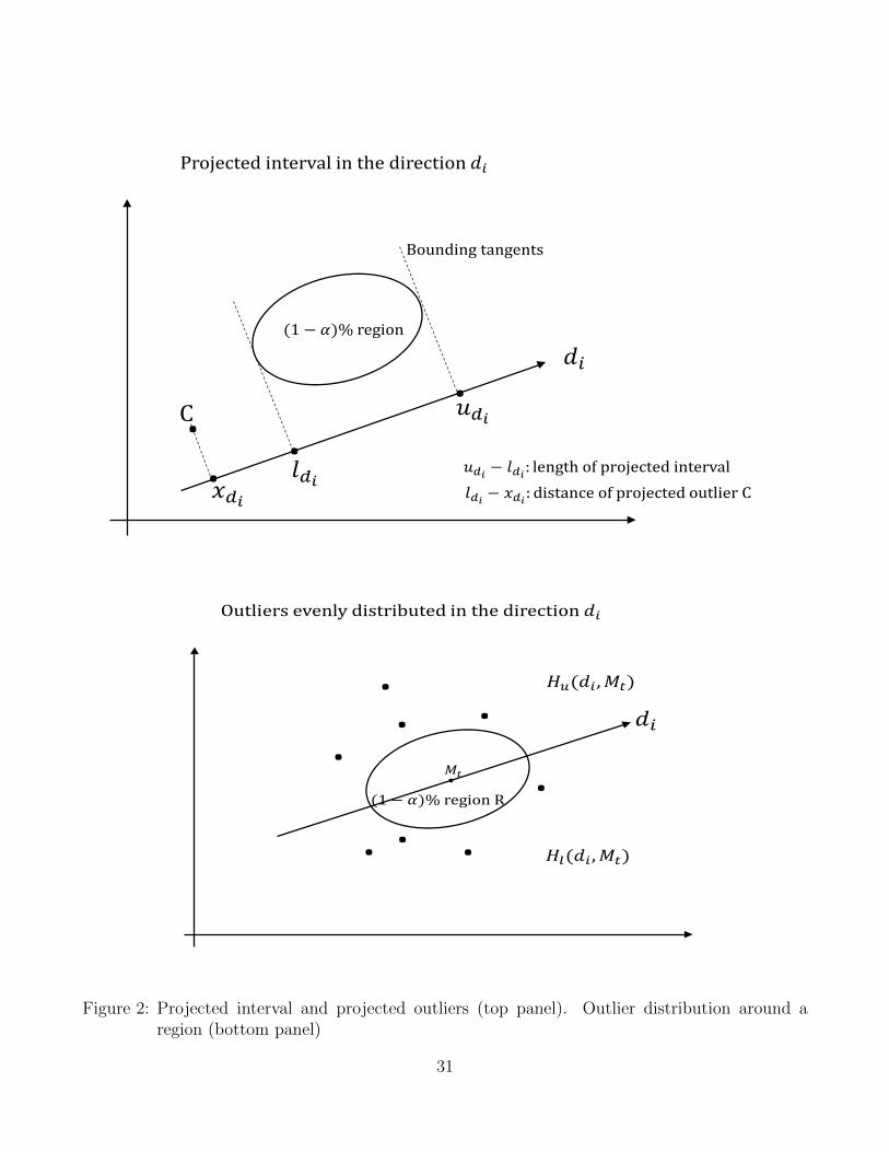
We also evaluate the prediction region by the sharpness or tightness of the intervals that result from
projecting the two-dimensional region into one-dimensional intervals. We draw a large number of
directions, which are given by the lines drawn from the zero origin of the unit circle to any point in
its boundary. For each direction, we find the two bounding tangent lines to the prediction region
that are perpendicular to that direction. We calculate the length of the projected interval bounded
by the tangent lines; see Figure 2 (top panel) for a graphical representation. Denote di ∈ Υ as the
ith direction in Υ, where Υ is the set of all directions, and let D be the number of directions. The
average length of the projected intervals associated with the prediction region is
P(1−α) =1
N
N∑t=1
Pt (4.4)
where Pt is the average projection length over all directions at time t given by Pt = 1D
∑Di=1(udi−ldi)
with udi and ldi being the upper and lower bounds of the projected interval in the ith direction. The
forecaster would prefer prediction regions that deliver tight projected intervals. We also consider
the realized data points over the prediction period in conjunction with the projected intervals.
The average distance of the projected outliers associated with the prediction region is
OP(1−α) =1
N
N∑t=1
OPt (4.5)
where OPt is the average distance of the projected outliers to the projected interval given by OPt =
1D
∑Di=1[(ldi − xdi)I(xdi < ldi) + (xdi − udi)I(xdi > udi)] with xdi being the coordinate of the data
point projected on the ith direction and I(•) being an indicator function. The forecaster prefers
13
prediction regions with projected outliers close to the projected intervals. Finally, if the length of
the projected interval is large, we expect the distance of the projected outliers to the interval to
be smaller. To take into account this trade-off, we propose a combined criteria POPt = Pt ×OPt
so that, over the prediction sample, the average trade-off associated with the prediction region is
POP(1−α) =1
N
N∑t=1
POPt (4.6)
A smaller POP(1−α) would be preferred by the forecaster.
Our final assessment of prediction regions is whether they are probability-centered. We check
whether the points outside of the prediction region are evenly distributed around the region R. In
this case, we expect the following statistic to be close to zero
S(1−α)(Mt) =1
D
D∑i=1
|Cu(di,Mt))− Cl(di,Mt)| (4.7)
where D is the number of directions that pass through Mt, Cu(di,Mt)) = #x|(x ∈ Rc) ∩ (x ∈
Hu(di,Mt)) and Cl(di,Mt) = #x|(x ∈ Rc) ∩ (x ∈ Hl(di,Mt)) with Hu(di,Mt) being the half-
plane above the line generated by the direction di, Hl(di,Mt) being the half-plane below the
same line and Rc the complementary region to R; see Figure 2 (bottom panel) for a graphical
representation. Note that S(1−α)(Mt) will not be feasible with real data (we will have only one
realized observation at time t that could be in or out of the prediction region). However, in a
simulated environment, we will be able to assess whether each prediction region is probability-
centered.
5 Monte Carlo Simulations
In this section, we perform Monte Carlo simulations to evaluate the prediction regions for interval
valued time series according to the criteria described in Section 4. We report just one case for
14
small samples here and extensive simulation cases in the supplementary material.
We generate R = 500 replicates of the center/log-range system from a VAR(4) with T = 50
observations and its parameters chosen to replicate the dynamics of S&P500 interval returns. The
center and log-range errors are distributed according to a Skewed-Student-t with 5 degrees of
freedom and asymmetry parameter -0.5 and a normal distribution, respectively.8 Note that the
distributional assumptions are on the marginal densities of the errors of each equation and we
do not know the exact bivariate densities. For the system to have the desired marginal density
functions and the stated correlation structure, we have generated bivariate errors from a Gaussian
copula and re-transform the PITs of the corresponding univariate normal variates according to the
Student-t, to obtain the new error variates, which need to be adjusted to have the desired mean and
variance. We construct one-step-ahead prediction regions with 95% nominal coverage and simulate
1000 future values of the required vector at time T + 1, i.e. center/log-range, center/range, and
upper/lower bounds. The empirical coverage is calculated as the proportion of these values that
falls within the constructed prediction regions. The number of bootstrap samples is B = 2000,
and the number of directions to calculate the average length of the projected intervals and outliers
is D = 100.9
Table 1 reports the evaluation criteria for the Monte Carlo experiments when the prediction regions
are constructed by all procedures described in Section 2 for the three systems (center/log-range,
center/range and upper/lower bounds). First, note that regardless of the particular system being
forecast, the regions based on the normality assumption for the center/log-range system have cov-
erages below the 95% nominal and their coverage-volume scores, CV, are nearly double than those
of the regions based on bootstrap procedures. Therefore, it seems that in cases of small samples
and/or non-Gaussian interval data, bootstrap procedures should be used instead of relaying on
normality. Comparing the alternative bootstrap regions considered, we can observe that bootstrap
8The Skewed-Student distribution is defined as proposed by Hansen (1994).9The parameters of the VAR(4) model are reported in the Supplementary material available online. Results for
other VAR models, error distributions and sample sizes are also reported in the Supplementary material.
15
ellipsoid have minimum coverage-volume scores, although the differences among them are very
small. However, the average outlier distance, O, is lower for the Tukey regions than for the other
bootstrap regions. When constructing the regions for the upper/lower bounds, the Tukey convex
hull has also smaller trade-off between sharpness and risk, POP and centeredness. Therefore, it
seems that in the presence of asymmetric distributions as that considered in this paper, the Tukey
convex hull provide adequate regions for interval data.
6 Prediction regions for S&P500 low/high returns
In this section, we construct joint prediction regions for the center (level) and log-range (volatility)
of daily S&P500 return intervals that take into account their interaction without making particular
assumptions on their joint distribution.
6.1 Joint modeling of returns and volatilities
Several authors propose modeling the interaction between volatility and asset returns fitting bi-
variate models to returns and realized variances. Among them, Takahasi et al. (2009) propose
an Stochastic Volatility model in which both returns and realized variances depend on a latent
volatility. The presence of this latent volatility force the authors to estimate the models and ex-
tract the volatility using computationally intensive Bayesian procedures. Shephard and Sheppard
(2010) also propose modeling returns and realized volatilities by fitting a VAR model called High-
frequency-based-volatility (HEAVY) and obtain the entire predictive distribution of returns based
on drawing with replacement pairs from the joint distribution of standardized returns and realized
volatilities. More recently, Catania and Proietti (2019) propose bivariate score driven models for
returns and realized volatilities.
The methodology proposed in this paper has several advantages with respect to bivariate models
for returns and realized volatilities. First, we avoid issues related to microstructure noise associated
16
with the construction of realized volatilities. As mentioned in the Introduction, several authors
advocate using the range as a measure of volatility. Second, using bootstrap prediction regions,
we avoid potential unrealistic assumptions about the joint distribution of returns and volatilities;
see, for example, Catania and Proietti (2019) who assume that returns and log-volatilities have
a joint Student-t distribution with ν degrees of freedom implying that the marginal univariate
distributions of returns and volatilities are both Student-t with ν degrees of freedom. Third, the
proposed methodology is a natural framework to incorporate other stylized facts as, for example,
the effect of past volatilities on returns. Last but not least, the proposed methodology is com-
putationally less intensive than alternative approaches and thus, it allows for a straightforward
implementation and can be easily extended to other models for the center/log-range system as
VARMA or cointegrated systems.
6.2 Model estimation
We collect intervals of low/high S&P500 prices, (PLt , P
Ut ) observed daily from January 2, 2009 to
April 20, 2018 for a total of 2341 observations. Since prices are non-stationary, we construct daily
stationary intervals of low/high returns, (yLt , yUt ) by calculating the daily minimum and maximum
return with respect to the closing price of the previous day, i.e. yLt = PLt −PC
t−1 and yUt = PUt −PC
t−1,
where PCt is the closing price at day t. Figure 3 (top panel), which plots a kernel estimate of the
bivariate unconditional density of the center and the range, shows that the center exhibits fat tails
and it is slightly skewed to the left. Furthermore, according to the sample descriptive statistics
reported in the Supplementary material, we can observe that the log-range is only slightly skewed
to the right and has a coefficient of kurtosis of about 3. The correlation between the center and
log-range is about -0.10. With respect to temporal dependence, as expected, the Q-statistics
for the center indicate no autocorrelation while those for the range and log-range indicate high
autocorrelation mimicking the autocorrelations often observed in the end-of-the day returns and
in their squared returns, respectively.
17
We split the total sample into an estimation sample from January 2, 2009 to December 31, 2016
(2014 observations) and a prediction/evaluation sample from January 1, 2017 to April 20, 2018
(327 observations). Using the estimation sample, we obtain the following LS estimates of the
(significant) parameters of a VAR(6) model as selected by the SIC criteria (robust standard errors
in parenthesis)10
Ct = 0
logRt = −0.17(0.013)
Ct−1 − 0.09(0.014)
Ct−2 − 0.06(0.014)
Ct−3 − 0.04(0.014)
Ct−4+
+ 0.17(0.023)
logRt−1 + 0.22(0.023)
logRt−2 + 0.16(0.023)
logRt−3 + 0.09(0.023)
logRt−4 + 0.1(0.023)
logRt−5 + 0.11(0.022)
logRt−6
As expected, all regressors (lagged center and lagged log-range) in the equation for the center are
not statistically significant. On the contrary, the equation for the log-range presents interesting
dynamics. The center Granger-causes the log-range so that the lagged centers are negatively
correlated with the current log-range, i.e. positive and large changes in the center return today
predict a narrower range tomorrow. This is similar to the leverage effect in a conditional variance
equation. Another relevant aspect, in agreement with the ACF/PACF profiles, is the strong and
statistically significant autoregressive nature of the log-range. The estimated VAR model captures
the main stylised facts often observed in financial returns: i) persistence of volatility; ii) heavy
tails of returns; and iii) negative dependence between volatility and past returns. The goodness
of fit for the log-range equation is high with an adjusted R2 = 0.52. In the Supplementary
Material, we report the results of the residual diagnosis. First, we observe that the residuals are
all clear of any autocorrelation. Furthermore, the center residuals and log-range residuals are
contemporaneous negatively correlated with a correlation coefficient of -0.17. Finally, we formally
test for conditional bivariate normality by implementing the Generalized AutoContouR (G-ACR)
(in-sample) tests based on the Probability Integral Transformations (PIT) of the joint density under
the null hypothesis of bivariate normality (Gonzalez-Rivera and Sun, 2015). We also report the
results of the t-statistics (tk,α) that canvas the density from the 1% to the 99% PIT autocontours
10Only significant values are reported.
18
for lags k = 1, 2, ...5. The null hypothesis is strongly rejected at the 5% significance level for
mostly all but the 10%, 90% and 95% autocontours. The portmanteau test Ck also reinforces
the strong rejection of bivariate normality. Figure 3 (bottom panel) plots the autocontours of the
contemporaneous PITs (centert, log-ranget). Under the correct null hypothesis, the distribution of
the PITs should be uniformly distributed within these autocontour squares. It is obvious that this
is not the case.
6.3 Out-of-sample forecast regions
We evaluate the out-of-sample performance of the one-step-ahead 95% prediction regions from
January 1, 2017 to April 20, 2018 (327 observations). The results are reported in Table 2. For the
system center/log-range, the bootstrap MBR regions offer the best coverage C with empirical rates
of mostly 95% and they are the most reliable with the lowest average coverage-volume scores CV .
They also provide the tightest projected one-dimensional regions measured by POP . However,
the Tukey convex hull regions provide the lowest average outlier distance O. For the system
center/range, we find that the transformed modified bootstrap Bonferroni rectangle is the best
performer according to most metrics C, CV and POP . For the system upper/lower bounds, the
Tukey convex hull offers the best coverage and the lowest scores for O and POP . As expected,
the analytic methods are not reliable as they tend to undercover. On the contrary, the bootstrap
ellipse and its transformed region tend to overcover. All these results are very consistent with the
Monte Carlo findings of the previous section.
In Figures 4 and 5, we plot the one-step-ahead 95% prediction regions for the center/log-range and
center/range systems respectively. We choose six random dates over the prediction sample (March
15, May 11, August 30, December 8, 2017 and February 22, April 6, 2018). In all six dates, the
one-step-ahead realized values of the (center, log-range) and (center, range) fall within the regions;
only the realized values on December 8, 2017 and April 6, 2018 are slightly more extreme and they
19
fall towards the boundaries of the prediction regions. For the center/log-range system, the normal
ellipse and the bootstrap ellipse are very similar but in the center/range system, the bootstrap
ellipse tends to be wider adapting to the kurtosis of the center and the asymmetry of the range.
The differences among the Bonferroni rectangles are more obvious in the center/range system. In
the center/log-range system, the Tukey convex hull has a cone shape over all the six dates though
the shape becomes more irregular in the center/range system.
It is important to point out that when using point data, we can obtain a single forecast density for
future returns. However, by using interval data, we are able to provide a wider characterization
of returns by constructing the conditional forecast density of returns conditioning on volatility or
the joint bivariate density of returns and volatilities.
6.4 Trading strategy
Using the bootstrap prediction regions for the daily S&P500 high/low returns obtained in the
previous section, we develop a trading strategy for interval data that extends that proposed by He
et al. (2010) for point forecasts. The proposed trading strategy exploits the probability distribution
of forecasts. Consider the following ratio st =|Ot−yl,t+h||yu,t+h−Ot| , where Ot is the opening return at day
t, calculated using the opening price at day t with respect to the closing price at day t − 1 and
yl,t+h and yu,t+h are the low and high return forecasts, respectively. If st < 1, then the return
is more likely to go up than down in the next h days. If this is observed for several days, it is
reasonable to believe that the market is forming an upward trend and a “buy alert signal” should
be generated. A similar argument can be applied to the “sell alert signal”. While He et al. (2010)
compute st using point forecasts of yu,t+h and yl,t+h, we compare the probability of st > 1 (sell
signal) and st < 1 (buy signal). Figure 6 illustrates the proposed trading strategy. Notice that st
is the absolute value of the slope of any line that connects point A ≡ (Ot, Ot) and any other point
below the 45 degree line. The ellipse represents the h-step-ahead prediction region of the high/low
20
returns. The slope of line AB is equal to (minus) one and it is perpendicular to the 45 degree
line. Hence, the area under the 45 degree line is divided into two areas by the line AB into two
areas: st > 1 to the left of line AB, and st < 1 to the right of line AB. Therefore, counting the
bootstrap realizations in the two subareas of the prediction region, we can compare the estimated
probability of st < 1 with that of st > 1 for a given 100× (1− α)% confidence region. Then, the
trading strategy consists of the following steps:
• At day t, plot Figure 6 based on Ot and the h-step-ahead prediction region of high and low
returns. Within the prediction region, if the number of bootstrap realizations (obtained as
in equation (3.4)) on the right hand side of the line AB is larger than that on the left hand
side of the line AB, a “buy alert signal” is generated.
• If Prob(st < 1) > Prob(st > 1) is observed for m consecutive days beginning with day t, buy
the asset on day t+m− 1 using the closing price on that day.
• After buying the asset, on any other day d, watch for the“sell alert signal”, that is, the
number of bootstrap realizations on the left hand side of the line AB should be larger than
that on the right hand side of the line AB within the prediction region. If the “sell alert
signal” is observed for m consecutive days from day d, sell the asset on day d+m− 1 using
the closing price on that day. Otherwise, hold the asset.
We evaluate this trading strategy over the out-of-sample period (Jan. 1, 2017 to Apr. 20, 2018)
using the bootstrap ellipse and Tukey Convex Hull prediction regions with a 95% nominal cover-
age. For the implementation, the choice of m should not be too small because it will introduce
substantial noise in trading but it should not be too large either because we could miss profitable
trades. We consider m = 1, 2, 3, 4 and h = 1, 2, 3. We apply a transaction cost of 0.1%, and we
annualize the profit/loss for each trade because each trade will have a different holding period.
The annualized return is calculated as ARt = (yc,t+j−yc,t
yc,t−0.001)(365
j) where yc,t and yc,t+j, (j > 0),
are the closing prices for the buying and selling days, respectively. The investor can buy the asset
21
again before the previous bought asset is sold. At the end of the evaluation period, if there are still
assets that have not been sold, these assets will not be considered when calculating the profits.
Table 3 reports the average and the max and min of ARt together with the percentage of trades
with positive returns for all cases. HKW is the trading strategy in He et. al. (2010) based on
point forecasts of the high/low returns. For all cases but two, the averaged annualized returns are
positive. The choice of m is very relevant because the gap between the max and min annualized
returns narrows as m increases for all h. A large m means that the investor is looking for a
stronger signal and, though she may miss some trades with extreme positive returns, she will also
avoid those extreme negative returns that can be catastrophic. There is also a monotonic positive
relation between m and the percentage of trades with positive returns. For average annualized
returns, the performance of BE is better than that of TH in most cases, and the performance of
BE or TH is better than HKW in particular when m = 4.
7 Conclusions
Often time series interval measurements offer a more complete description of a data set because
each observation has joint information on the level and the dispersion of the process under study.
However, statistical analysis of interval-valued data requires that the natural order of the interval is
preserved. Though there are several works that consider the problem of estimation with constraints,
we are not aware of any work that considers the construction of probabilistic forecasts for interval-
valued data satisfying the natural constraint in each period of time. Our contribution lies on
approximating a probabilistic forecast of an interval-valued time series by offering alternative
approaches to construct bivariate prediction regions of the center and the range, or the lower and
upper bounds, of the interval.
To overcome the positive constraint of the range, we estimate a Gaussian bivariate system for
the center/log-range system, which delivers QML properties for our estimators. However, the
22
interest of the researcher is not the prediction of the center/log-range but the center/range or
upper/lower bounds of the interval. By implementing either analytical or bootstrap methods
we directly transform the prediction regions for the center/log-range system into those for the
center/range and upper/lower bounds systems. It is important to remark that we do not focus on
point forecast purposely. By focusing on prediction regions rather than on point forecasts, we avoid
the biases associated with the exp-transformation of the point forecasts of log-transformed variable.
A prediction region for the center/log-range does not need any bias correction when transformed
into a prediction region of the center/range system because the quantile is preserved under a
monotonic transformation like the exp-transformation. These transformed prediction regions can
have very irregular shapes even in the most straightforward scenario of bivariate normality of
the center/log-range system. If a central point forecast is of interest, the researcher can always
calculate the centroid of the region.
Beyond the standard coverage rate, we propose several new metrics to evaluate the performance
of prediction regions. We introduce a notion of risk to the evaluation of the regions by considering
the location of the out-of-the-region outcomes with respect to some central point in the region.
The researcher would like to minimize risk once the empirical coverage of the region is close to
the nominal coverage. We have considered Gaussian and non-Gaussian systems and our recom-
mendation leans towards bootstrap methods, even for Gaussian systems. Bootstrap ellipses and
their transformed are best when the joint distribution of the center/log-range system is symmet-
ric. If it is not, then bootstrap Tukey hull regions will be preferred. In summary, we find that
simulation-based methods are the most reliable.
We analyze a time series of the daily low/high return intervals of the S&P500 index. We model
and predict the joint conditional density of the return level and volatility. We show that the
bootstrap regions have best properties. Furthermore, we carry out a trading strategy to illustrate
the economic advantages of taking into account the probabilistic forecast of the low/high returns
23
instead of point forecasts.
References
[1] Alizadeh, S., M. W. Brandt, & F.X. Diebold (2002). Range-based Estimation of StochasticVolatility Models. Journal of Finance, 57(3), pp. 1047-1091.
[2] Beran, R. (1993). Probability-Centered Prediction Regions. Annals of Statistics, 21(4), pp.1967-1981.
[3] Bien, K., I. Nolte & W. Pohlmeier (2011). An inflated multivariate integer count hurdlemodel: An application to bid and ask quote dynamics. Journal of Applied Econometrics, 26,pp. 669-707.
[4] Blasques, F., S.J. Koopman, K. Lasak & A. Lucas (2016). In-sample confidence bands andout-of-sample forecast bands for time-varying parameters in observation-driven models. In-ternational Journal of Forecasting, 32, pp. 875-887.
[5] Brandt, M.W. & F.X. Diebold (2006). A no-arbitrage approach to range-based estimation ofreturn covariance and correlations. Journal of Business, 79, pp. 61-74.
[6] Catania, L., & T. Proietti (2019). Forecasting volatility with time-varying leverage and volatil-ity effects. CEIS Tor Vergata Research Paper Series, Vol. 17, issue 1, no.450.
[7] Clements, M.P. & J. Smith (2002). Evaluating multivariate forecast densities: a comparisonof two approaches. International Journal of Forecasting, 18(3), pp. 397-407.
[8] Cheung, Y.L., Y.W. Cheung, & A.T. Wan (2009). A high-low model of daily stock priceranges. Journal of Forecasting, 28(2), pp. 103-119.
[9] Diebold, F.X., A. Han & K. Tay (1999). Multivariate density forecast evaluation and cali-bration in financial risk management: High-frequency returns on foreign exchange. Review ofEconomics and Statistics, 81(4), pp. 661-673.
[10] Fernandez, C., Leon, C.J., Steel, M.F.J., & Vazquez-Polo, F.J. (2004). Bayesian analysis of in-terval data contingent valuation models and pricing policies. Journal of Business & EconomicStatistics, 22(4), pp. 431-442.
[11] Fresoli, D., E. Ruiz, & L. Pascual (2015). Bootstrap Multi-step Forecasts for Non-GaussianVAR Models. International Journal of Forecasting, 31, pp. 834-848.
[12] Garcıa-Ascanio, C. & C. Mate (2010). Electric power demand forecasting using interval timeseries: A comparison between VAR and iMLP. Energy Policy, 38(2), pp. 715-725.
[13] Gneiting, T., L.I. Stanberry, E.P. Grimit, L. Held & N.A. Johnson (2008). Assessing prob-abilistic forecasts of multivariate quantities, with an application to ensemble prediction ofsurface winds. TEST, 17(2), pp. 211-235.
24
[14] Golestaneh, F., P. Pinson, R. Azizipanah-Abarghooee, & H.B. Gooi (2018). Ellipsoidal Pre-diction Regions for Multivariate Uncertainty Characterization. IEEE Transactions on PowerSystems, 33(4), pp. 4519-4530.
[15] Gonzalez-Rivera, G., & W. Lin (2013). Constrained Regression for Interval-valued Data. Jour-nal of Business and Economic Statistics, 31(4), pp. 473–490.
[16] Gonzalez-Rivera, G., & Y. Sun (2015). Generalized Autocontours: Evaluation of MultivariateDensity Models. International Journal of Forecasting, 31(3), pp. 799-814.
[17] Gonzalez-Rivera, G., & E. Yoldas (2011). Autocontour-based evaluation of multivariate pre-dictive densities. International Journal of Forecasting, 28(2), 328-342.
[18] Granger, C.W.J. & P. Newbold (1976). Forecasting Transformed Series. Journal of the RoyalStatistical Society, B, 38, pp. 189-203.
[19] Guerrero, V.M. (1993). Time Series Analysis Supported by Power Transformation. Journal ofForecasting, 12, pp. 37-48.
[20] Han, A., Y. Hong & S. Wang (2016). Autoregressive conditional models for interval-valuedtime series data. In R. Hill, G. Gonzalez-Rivera & T. Lee (eds.), Advances in Econometrics,vol. 36, Emerald Group Publishing Limited, pp. 417-460.
[21] Hansen, B.E. (1994). Autoregressive conditional density estimation. International EconomicReview, 35(3), pp. 705-730.
[22] He, A.W.W., J.T.K. Kwok & A.T.K. Wan (2010). An empirical model of daily highs and lowsof West Texas intermediate crude oil prices.Energy Economics, 32, pp. 1499-1506.
[23] Ji, S. & X. Shi (2018). Reaching goals under umbiguity: Continuous-time optimal portfolioselection.Statistics and Probability Letters, 137, pp. 63-69.
[24] Komunjer, I. & M. Owyang (2012). Multivariate forecast evaluation and rationality test-ing.Review of Economics and Statistics, 94(4), pp. 1066-1080.
[25] Lima Neto, E. & F. de Carvalho (2010). Constrained Linear Regression Models for SymbolicInterval-Valued Variables. Computational Statistics and Data Analysis, 54, pp. 333-347.
[26] Lin, W. & G. Gonzalez-Rivera (2016). Interval-valued time series models: estimation basedon order statistics exploring the Agriculture Marketing Service data. Computational Statistics& Data Analysis, 100, pp. 694-711.
[27] Lutkephol, H. (1991). Introduction to Multiple Time Series Analysis, Springer-Verlag, Berlin.
[28] Manski, C.F, & E. Tammer (2002). Interence on regressions with interval data on a regressoror outcome. Econometrica, 70(2), pp. 519-546.
[29] Parkinson, M. (1980). The Extreme Value Method for Estimating the Variance of the Rateof Return. Journal of Business, 53(1), pp. 61-65.
25
[30] Pascual, L., J. Romo & E. Ruiz (2005). Bootstrap Prediction Intervals for Power TransformedTime Series. International Journal of Forecasting, 21, pp. 219-235.
[31] Pascual, R. & D. Veredas (2010). Does the open limit order book matter in explining infor-mational volatility?. Journal of Financial Econometrics, 8(1), pp. 57-87.
[32] Rodrigues, P. & N. Salish (2015). Modelling and forecasting interval time series with thresholdmodels. Advances in Data Analysis and Classification, 9, pp. 41-57.
[33] Rogers, L.C.G. & S.E. Satchell (1991). Estimating variance from high, low and closing prices.Annals of Applied Probability, 1(4), pp. 504-512.
[34] Rogers, L.C.G., S.E. Satchell & Y. Yoon (1994). Estimating the volatility of stock prices: acomparison of methods that use high and low prices. Applied Financial Economics, 4, pp.241-247.
[35] Shephard, N. & K. Sheppard (2010). Realising the future: Forecasting with high-frequency-based volatility (HEAVY) models. Journal of Applied Econometrics, 25, pp. 197-231.
[36] Takahashi, M., Y. Omori and T. Watanabe (2009). Estimating stochastic volatility modelsusing daily returns and realized volatility simultaneously. Computational Statistics and DataAnalysis, 53, pp. 2404-2426.
[37] Tu, Y. & Y. Wang (2016). Center and Log Range Models for Interval-valued Data with AnApplication to Forecast Stock Returns. Working paper.
[38] Tukey, J. (1975). Mathematics and Picturing Data, in Proceedings of the 1975 InternationalCongress of Mathematics, 2, pp. 523-531.
[39] Vorbrink, J. (2014). Financial markets with volatility uncertainty. Journal of MathematicalEconomics, 53, pp. 64-78.
[40] Xiong, T., Y. Bao, Z. Hu & L. Zhang (2015). A combination method for interval forecastingof agricultural commodity futures prices. Knowledge-Based Systems, 77, pp. 92-102.
[41] Xiong, T., C. Li & Y. Bao (2017). Interval-valued time series forecasting using a novel hybridHolt and MSVR model. Economic Modelling, 60, pp. 11-23.
[42] Yao, W. & Z. Zhao (2013). Kernel Density-based Linear Regression Estimate. Communicationsin Statistics. Theory and Methods, 42(24), pp. 4499-4512.
[43] Yeh, A.B:, & Singh, K. (1997). Balanced confidence regions based on Tukey’s depth and thebootstrap. Journal of the Royal Statistical Society, Series B (Methodological), 59(3), 639-652.
[44] Zuo, Y. (2003). Projection-based Depth Functions and Associated Medians. Annals of Statis-tics, 31(5), pp. 1460-1490.
% of trades with positive returns 62.67% 58.97% 57.69% 80.77% 78.57% 77.78% 88.89% 71.43% 57.14% 100% 100% 100%
Table 3: Trading strategy comparison for S&P500 average annualized returns over the out-of-sample period from January 1, 2017 to April 20, 2018.
29
Figure 1: 95% prediction regions for the center/log-range system (top panel) and center/rangesystem (bottom panel) obtained from a simulated VAR(4) model with parameters: a1 =
−0.93, b(1)11 = 0.34, b
(2)11 = −0.15, b
(3)11 = 0.03, b
(4)11 = −0.06, b
(1)12 = −0.50, b
(2)12 = 0.13, b
(3)12 =
−0.16, b(4)12 = 0.92, a2 = 0.08, b
(1)21 = −0.01, b
(2)21 = b
(3)21 = b
(4)21 = 0, b
(1)22 = 0.09, b
(2)22 =
0.18, b(3)22 = 0.15, b
(4)22 = 0.08 and Gaussian errors with variances given by σ2
1 = 111.24and σ2
2 = 0.16 and covariance σ12 = −1.02. The sample size is T = 1000.
30
.. .
.𝑑𝑑𝑖𝑖
𝑢𝑢𝑑𝑑𝑖𝑖
𝑙𝑙𝑑𝑑𝑖𝑖𝑥𝑥𝑑𝑑𝑖𝑖𝑢𝑢𝑑𝑑𝑖𝑖 − 𝑙𝑙𝑑𝑑𝑖𝑖: length of projected interval𝑙𝑙𝑑𝑑𝑖𝑖 − 𝑥𝑥𝑑𝑑𝑖𝑖: distance of projected outlier C
C
(1 − 𝛼𝛼)% region
Bounding tangents
Projected interval in the direction 𝑑𝑑𝑖𝑖
.𝑀𝑀𝑡𝑡
𝑑𝑑𝑖𝑖
𝐻𝐻𝑢𝑢(𝑑𝑑𝑖𝑖 ,𝑀𝑀𝑡𝑡)
𝐻𝐻𝑙𝑙(𝑑𝑑𝑖𝑖 ,𝑀𝑀𝑡𝑡)
(1 − 𝛼𝛼)% region R
.
....
..
.
Outliers evenly distributed in the direction 𝑑𝑑𝑖𝑖
Figure 2: Projected interval and projected outliers (top panel). Outlier distribution around aregion (bottom panel)
31
0-4
0.1
0.2
0
0.3
0.4
0.5
SP500 Center and Range
0.6
Pro
babili
ty D
ensity
0.7
0.8
-2
0.9
2
CenterRange
0426
48
0 0.1 0.2 0.3 0.4 0.5 0.6 0.7 0.8 0.9 1
PIT (Center)t
0
0.1
0.2
0.3
0.4
0.5
0.6
0.7
0.8
0.9
1
PIT
(lo
g-R
ange|C
ente
r) t
SP500
Figure 3: Unconditional bivariate density (top panel) of S&P500 low/high return intervals andG-ACR specification tests for conditional bivariate normality of residuals of the centerand log-range VAR(6) model (bottom panel).
32
-4 -3 -2 -1 0 1 2 3 4
Center
-2
-1.5
-1
-0.5
0
0.5
1
1.5
2
2.5
3
log
-Ra
ng
e
SP500 (One step ahead prediction regions)
realized one-step ahead values
Normal ellipse
Bonferroni rectangle
Modified Bonferroni rectangle
Bootstrap ellipsoid
Bootstrap Bonferroni rectangle
Modified Bootstrap Bonferroni rectangle
Tukey Convex Hull
Forecast period: Mar 15, 2017
-4 -3 -2 -1 0 1 2 3 4
Center
-2
-1.5
-1
-0.5
0
0.5
1
1.5
2
2.5
3
log
-Ra
ng
e
SP500 (One step ahead prediction regions)
realized one-step ahead values
Normal ellipse
Bonferroni rectangle
Modified Bonferroni rectangle
Bootstrap ellipsoid
Bootstrap Bonferroni rectangle
Modified Bootstrap Bonferroni rectangle
Tukey Convex Hull
Forecast period: May 11, 2017
-4 -3 -2 -1 0 1 2 3 4
Center
-2
-1.5
-1
-0.5
0
0.5
1
1.5
2
2.5
3
log
-Ra
ng
e
SP500 (One step ahead prediction regions)
realized one-step ahead values
Normal ellipse
Bonferroni rectangle
Modified Bonferroni rectangle
Bootstrap ellipsoid
Bootstrap Bonferroni rectangle
Modified Bootstrap Bonferroni rectangle
Tukey Convex Hull
Forecast period: Aug 30, 2017
-4 -3 -2 -1 0 1 2 3 4
Center
-2
-1.5
-1
-0.5
0
0.5
1
1.5
2
2.5
3
log
-Ra
ng
e
SP500 (One step ahead prediction regions)
realized one-step ahead values
Normal ellipse
Bonferroni rectangle
Modified Bonferroni rectangle
Bootstrap ellipsoid
Bootstrap Bonferroni rectangle
Modified Bootstrap Bonferroni rectangle
Tukey Convex Hull
Forecast period: Dec 8, 2017
-4 -3 -2 -1 0 1 2 3 4
Center
-2
-1.5
-1
-0.5
0
0.5
1
1.5
2
2.5
3
log
-Ra
ng
e
SP500 (One step ahead prediction regions)
realized one-step ahead values
Normal ellipse
Bonferroni rectangle
Modified Bonferroni rectangle
Bootstrap ellipsoid
Bootstrap Bonferroni rectangle
Modified Bootstrap Bonferroni rectangle
Tukey Convex Hull
Forecast period: Feb 22, 2018
-4 -3 -2 -1 0 1 2 3 4
Center
-2
-1.5
-1
-0.5
0
0.5
1
1.5
2
2.5
3
log
-Ra
ng
e
SP500 (One step ahead prediction regions)
realized one-step ahead values
Normal ellipse
Bonferroni rectangle
Modified Bonferroni rectangle
Bootstrap ellipsoid
Bootstrap Bonferroni rectangle
Modified Bootstrap Bonferroni rectangle
Tukey Convex Hull
Forecast period: Apr 6, 2018
Figure 4: One-step-ahead 95% prediction regions for the center/log-range system of the SP500 return intervals correspond-ing to different dates of the out-of-sample period.
33
-4 -3 -2 -1 0 1 2 3 4
Center
0
0.5
1
1.5
2
2.5
3
Ra
ng
e
SP500 (One step ahead prediction regions)
realized one-step ahead values
Analytical contour
Normal ellipse
Bonferroni rectangle
Modified Bonferroni rectangle
Bootstrap ellipsoid
Bootstrap Bonferroni rectangle
Modified Bootstrap Bonferroni rectangle
Tukey Convex Hull
Forecast period: Mar 15, 2017
-4 -3 -2 -1 0 1 2 3 4
Center
0
0.5
1
1.5
2
2.5
3
Ra
ng
e
SP500 (One step ahead prediction regions)
realized one-step ahead values
Analytical contour
Normal ellipse
Bonferroni rectangle
Modified Bonferroni rectangle
Bootstrap ellipsoid
Bootstrap Bonferroni rectangle
Modified Bootstrap Bonferroni rectangle
Tukey Convex Hull
Forecast period: May 11, 2017
-4 -3 -2 -1 0 1 2 3 4
Center
0
0.5
1
1.5
2
2.5
3
Ra
ng
e
SP500 (One step ahead prediction regions)
realized one-step ahead values
Analytical contour
Normal ellipse
Bonferroni rectangle
Modified Bonferroni rectangle
Bootstrap ellipsoid
Bootstrap Bonferroni rectangle
Modified Bootstrap Bonferroni rectangle
Tukey Convex Hull
Forecast period: Aug 30, 2017
-4 -3 -2 -1 0 1 2 3 4
Center
0
0.5
1
1.5
2
2.5
3
Ra
ng
e
SP500 (One step ahead prediction regions)
realized one-step ahead values
Analytical contour
Normal ellipse
Bonferroni rectangle
Modified Bonferroni rectangle
Bootstrap ellipsoid
Bootstrap Bonferroni rectangle
Modified Bootstrap Bonferroni rectangle
Tukey Convex Hull
Forecast period: Dec 8, 2017
-4 -3 -2 -1 0 1 2 3 4
Center
0
1
2
3
4
5
6
7
8
Ra
ng
e
SP500 (One step ahead prediction regions)
realized one-step ahead values
Analytical contour
Normal ellipse
Bonferroni rectangle
Modified Bonferroni rectangle
Bootstrap ellipsoid
Bootstrap Bonferroni rectangle
Modified Bootstrap Bonferroni rectangle
Tukey Convex Hull
Forecast period: Feb 22, 2018
-4 -3 -2 -1 0 1 2 3 4
Center
0
1
2
3
4
5
6
7
8
Ra
ng
e
SP500 (One step ahead prediction regions)
realized one-step ahead values
Analytical contour
Normal ellipse
Bonferroni rectangle
Modified Bonferroni rectangle
Bootstrap ellipsoid
Bootstrap Bonferroni rectangle
Modified Bootstrap Bonferroni rectangle
Tukey Convex Hull
Forecast period: Apr 6, 2018
Figure 5: One-step-ahead 95% prediction regions for the center/range system of the SP500 return intervals correspondingto different dates of the out-of-sample period.
34
.(𝑂𝑂𝑡𝑡, 𝑂𝑂𝑡𝑡)≡ A
𝐿𝐿𝑡𝑡+ℎ
𝑈𝑈𝑡𝑡+ℎ
(1 − 𝛼𝛼)% region
Trading strategy (buy and sell signals)
(𝑠𝑠 = 1)
(𝑏𝑏𝑢𝑢𝑏𝑏 𝑠𝑠𝑠𝑠𝑠𝑠𝑠𝑠𝑠𝑠𝑙𝑙: 𝑠𝑠 < 1)
(𝑠𝑠𝑠𝑠𝑙𝑙𝑙𝑙 𝑠𝑠𝑠𝑠𝑠𝑠𝑠𝑠𝑠𝑠𝑙𝑙: 𝑠𝑠 > 1)B
45 degree line
Figure 6: Buy and sell signals from trading strategy.


![Research Article Certain Types of Interval-Valued Fuzzy Graphsdownloads.hindawi.com/journals/jam/2013/857070.pdfis an interval-valued fuzzy set on and =[ , +] is an interval-valued](https://static.documents.pub/doc/80x56/5fe3268d15825b66b650f8f4/research-article-certain-types-of-interval-valued-fuzzy-is-an-interval-valued-fuzzy.jpg)


