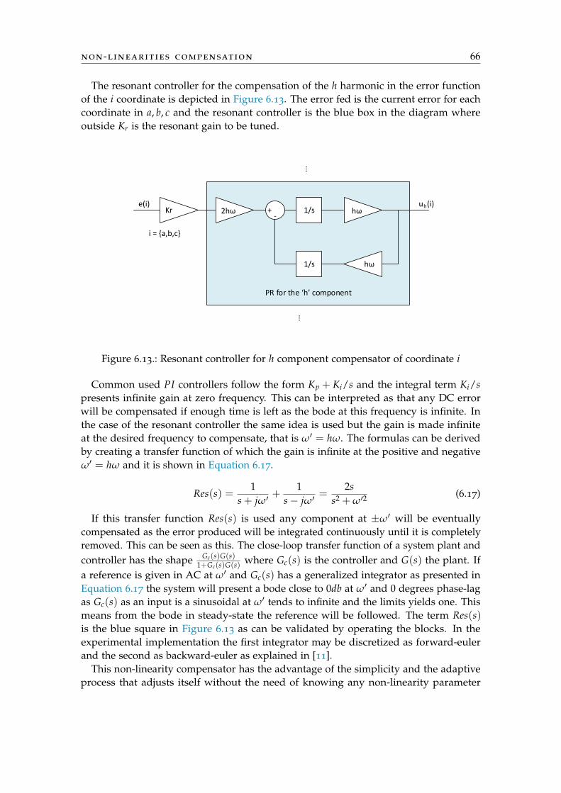
Predictive control for PMSM - Aalborg...

Predictive control for PMSM

Predictivecontroller

ConverterMachine(electrical)

Non-linearitiescompensator

Parameterestimator

++u* u'u

uNL

i

p

i*

Master’s ThesisPED4-944

Carlos Gómez Suárez

January 6, 2016

Title: Predictive control for PMSM

Semester: 3th-4th semester M.Sc.

Semester theme: Master thesis – Power Electronics and Drives

Project period: 01-02-2015 – 29-01-2016

ECTS: 50

Supervisor: Kaiyuan Lu

Project group: PED4-944

_____________________________________

Carlos Gómez Suárez

Copies: [0]

Pages, total: [135]

Appendix: [4]

Supplements: [1 CD]

By signing this document, each member of the group confirms that all group members have

participated in the project work, and thereby all members are collectively liable for the contents

of the report. Furthermore, all group members confirm that the report does not include

plagiarism.

SYNOPSIS:

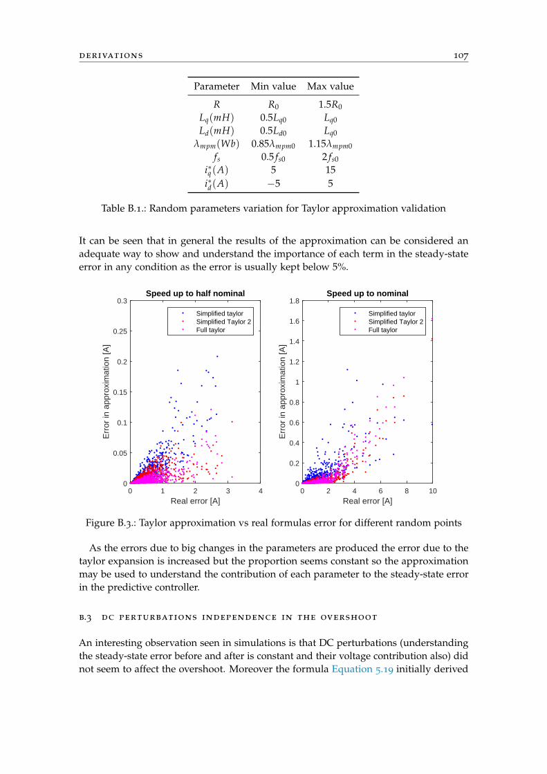
This thesis focuses in the design, analysis and implementation of a predictive current controller for the control of a Permanent Magnet Synchronous Machine (PMSM). This thesis studies the predictive controller including the main problems presented with its implementation. The effect of errors in the system parameters is studied and different non-linearities are analyzed and compensated. Online parameter estimations are also developed as a way for the compensator to adapt to changes in them. As a result of the thesis the predictive controller is seen as a simple controller with excellent performance when the different disturbances that affect the system are accounted for.

P R E FA C E

This master thesis is written by Carlos Gomez, a 10th master student in the Departmentof Energy Technology in Aalborg University. The semester theme is Power Electronicsand Drives.

Reading instructions The denotation of employed equations, figures, tables and codestrough the thesis is based in the notation (X.Y) which means the Yth item belonging tothe Xth chapter. The units used are placed on the right of the numbers and are usuallySI units.

At the end of the thesis the appendices can be found which supplement the informationprovided. Bibliography is placed after them. The references follow [k] where k representsthe k reference in the bibliography list. As a further attachment a CD with simulations isprovided as well as a PDF version of the thesis.

Publication of this thesis is allowed only with reference to and with permission givenby the author.

i

A B S T R A C T

This thesis focuses in the design, analysis and implementation of a predictive currentcontroller for the control of a Permanent Magnet Synchronous Machine (PMSM).

The theory regarding the PMSM and converter system is described mathematically inorder to have models to better understand the different problems. Trough the differentparts of the project several approximations are needed to yield solutions to the problemspresented and trough simulation and experiments the hypothesis taken are validated.

This thesis studies the predictive controller including the main problems presentedwith its implementation. The effect of changes in system parameters is studied and differ-ent non-linearities are analyzed and compensated. Finally online parameter estimationsare also developed as a way for the compensator to adapt to changes in them.

As a result of the thesis the predictive controller is seen as a simple controller withexcellent performance when the different compensations needed are accounted for.

ii

C O N T E N T S

1 introduction 1

1.1 Predictive control methods . . . . . . . . . . . . . . . . . . . . . . . . . . . 1

1.2 Problem statement . . . . . . . . . . . . . . . . . . . . . . . . . . . . . . . . 2

1.3 Objective . . . . . . . . . . . . . . . . . . . . . . . . . . . . . . . . . . . . . . 3

1.4 Thesis outline . . . . . . . . . . . . . . . . . . . . . . . . . . . . . . . . . . . 3

1.5 Limitations and assumptions . . . . . . . . . . . . . . . . . . . . . . . . . . 4

2 system description 6

2.1 System setup . . . . . . . . . . . . . . . . . . . . . . . . . . . . . . . . . . . . 6

2.2 Voltage source inverter . . . . . . . . . . . . . . . . . . . . . . . . . . . . . . 8

2.3 Permanent Magnet Synchronous Machine . . . . . . . . . . . . . . . . . . . 11

2.4 System parameters . . . . . . . . . . . . . . . . . . . . . . . . . . . . . . . . 15

3 field oriented control 17

3.1 Current control . . . . . . . . . . . . . . . . . . . . . . . . . . . . . . . . . . 17

3.2 Speed control . . . . . . . . . . . . . . . . . . . . . . . . . . . . . . . . . . . 19

3.3 Anti wind-up . . . . . . . . . . . . . . . . . . . . . . . . . . . . . . . . . . . 22

3.4 Simulation results . . . . . . . . . . . . . . . . . . . . . . . . . . . . . . . . . 22

3.5 Experimental results . . . . . . . . . . . . . . . . . . . . . . . . . . . . . . . 23

4 predictive current control 25

4.1 Description of the algorithm . . . . . . . . . . . . . . . . . . . . . . . . . . . 25

4.2 Angle compensation . . . . . . . . . . . . . . . . . . . . . . . . . . . . . . . 28



5 parameter sensitivity analysis 31

5.1 System model . . . . . . . . . . . . . . . . . . . . . . . . . . . . . . . . . . . 31

5.2 Stability . . . . . . . . . . . . . . . . . . . . . . . . . . . . . . . . . . . . . . . 35

5.3 Steady-state errors . . . . . . . . . . . . . . . . . . . . . . . . . . . . . . . . 40

5.4 Transient response . . . . . . . . . . . . . . . . . . . . . . . . . . . . . . . . 47

6 non-linearities compensation 54

6.1 Deadtime . . . . . . . . . . . . . . . . . . . . . . . . . . . . . . . . . . . . . . 54

6.2 Snubber compensation . . . . . . . . . . . . . . . . . . . . . . . . . . . . . . 57

6.3 Compensating diode and IGBT voltage drop . . . . . . . . . . . . . . . . . 60

6.4 Final compensator . . . . . . . . . . . . . . . . . . . . . . . . . . . . . . . . 63

6.5 Resonant controller compensation . . . . . . . . . . . . . . . . . . . . . . . 65



7 parameter determination 78

iii

Contents iv

7.1 Introduction . . . . . . . . . . . . . . . . . . . . . . . . . . . . . . . . . . . . 78

7.2 Recursive Least Square (RLS) . . . . . . . . . . . . . . . . . . . . . . . . . . 79

7.3 Gradient descent method . . . . . . . . . . . . . . . . . . . . . . . . . . . . 84

8 conclusions 89

8.1 Future work . . . . . . . . . . . . . . . . . . . . . . . . . . . . . . . . . . . . 90

Bibliography 91

Appendices 93

a offline parameter determination 94

a.1 Resistor estimation . . . . . . . . . . . . . . . . . . . . . . . . . . . . . . . . 94

a.2 Electrical machine parameters and non-linearities . . . . . . . . . . . . . . 95

a.3 Mechanical parameters . . . . . . . . . . . . . . . . . . . . . . . . . . . . . . 99

b derivations 102

b.1 Reference frame derivation . . . . . . . . . . . . . . . . . . . . . . . . . . . 102

b.2 Taylor derivation to approximate steady-state errors . . . . . . . . . . . . . 105

b.3 DC perturbations independence in the overshoot . . . . . . . . . . . . . . 107

b.4 Proof of convergence of gradient method in PMSM . . . . . . . . . . . . . 110

c model’s diagrams 112

c.1 System model . . . . . . . . . . . . . . . . . . . . . . . . . . . . . . . . . . . 112

c.2 Control scheme . . . . . . . . . . . . . . . . . . . . . . . . . . . . . . . . . . 112

c.3 Deadtime . . . . . . . . . . . . . . . . . . . . . . . . . . . . . . . . . . . . . . 115

c.4 Parameter estimation . . . . . . . . . . . . . . . . . . . . . . . . . . . . . . . 115

d list of codes 117

d.1 Predictive controller . . . . . . . . . . . . . . . . . . . . . . . . . . . . . . . 117

d.2 Non-linearity compensation (analytical) . . . . . . . . . . . . . . . . . . . . 119

d.3 Parameter determination . . . . . . . . . . . . . . . . . . . . . . . . . . . . . 124

1I N T R O D U C T I O N

Development of semiconductor devices and powerful cost efficient Digital Signal Process-ing (DSP)s give opportunities for applications in different areas including AC-machinedrives.

Permanent Magnet Synchronous Machine (PMSM) drives present several advantagesover other drives due to its high efficiency and high power density capabilities. Thecontrol of this drives can be performed trough vector control which was developed as away to get better torque responses trough the decoupling of the system in two differentcontrols, one for the torque and one for the flux [1]. This is illustrated in Figure 1.1. Thefocus of the project consist in the inner loop or current controller.

Speed controllerMechanical

SystemCurrent

ControllerElectricalSystem

w* i*+

-+

-

Figure 1.1.: System controllers

The flux, controlled by the field current can be performed trough the conventional useof PI controllers which offer a simple solution to the problem. However the transientresponse can be improved with different techniques which have been studied over theyears from which predictive controller is a promising method.

1.1 predictive control methods

Predictive controllers use models of the system to create predictions of future statesand variables to control. With this information the actuation in the system is obtainedaccording to the method used. Several classifications can be made as suggested in [2].The main strategies are: hysteresis based, trajectory based, model predictive control(MPC) and deadbeat.

Hysteresis based which needs no modulator bounds control variables within a tol-erance band and calculates the instants at which the switch states must change. Thisrequires a variable frequency.

Trajectory based calculates different optimum control strategies based in differentstates and applies them directly. There is no need for cascade control and speed canbe controlled directly from the speed error without a current controller. The switchingstates of the converter are classified into categories such as "increasing torque", "reducingtorque slowly", etc. and the instants to change are also calculated so variable frequencyis needed.

1

introduction 2

Model predictive control can use modulators (and fixed switching frequency) depend-ing of the implementation or a finite control set where the different switching states aretried within an horizon. A cost function with the errors between variables is created andoptimized by modifying the different control variables trough an optimization algorithm.In the case of finite set for example the 8 different switching states can be tested to seewhich one produces the best (least error in the optimization function) response in thenext period.

Finally deadbeat controller uses a modulator (and fixed frequency) for the currentcontroller. Based on system equations the voltage to apply to reach the current referenceis estimated.

Based in the main principles of the controllers and previous work conducted in [3] -[4] deadbeat controller is chosen. In [4] both MPC and deadbeat are implemented. MPCis observed to present a much bigger ripple in the current due to the lack of modulator,simple switching strategy and sampling frequency of 25 kHz imposed as a limit by thesetup. Deadbeat is only worse in steady-state errors due to simulated system parameterchanges. In [3] deadbeat controller presents also good results.

1.2 problem statement

A PMSM can be controlled by means of two different set of controllers as shown inFigure 1.1. The outside loop regulates the speed by adjusting the current that passestrough the motor as this modifies the electrical torque which in the end modifies thespeed.

On the other hand, inside a current loop (blue rectangle) regulates the voltage appliedto the motor in order to achieve the desired current. This project is focused in this secondcontroller. The speed controller used may be a PI while a predictive controller that usesthe machine equations to obtain a better response is studied in this project in contrast tothe classical PI for current control


ConverterMachine(electrical)

Non-linearitiescompensator

Parameterestimator

++u* u'u

uNL

i

p

i*

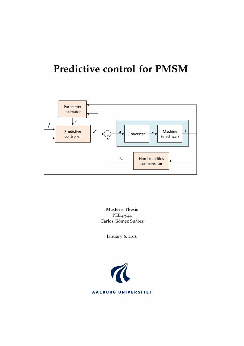
Figure 1.2.: Predictive current controller, non-linearity compensation and online parame-ter estimator represented in blocks

introduction 3

Further study of the electrical system shows that there are 3 main problems to solve asshown in Figure 1.2 (pink rectangles) in which the project will have its focus:

• Predictive controller: Using models that predict different states a control can bemade with great performance relying on the predictions of the variables.

• Non-linearity compensation: Since the predictive controller uses models of thesystem everything needs to be accounted for in order to compensate for it. When avoltage command is sent to the converter it is converted from u to u′ as illustratedin Figure 1.2 and can be compensated by adding an extra voltage uNL to accountfor it. The non-linearities studied in this project are the deadtime in the gate signalsand the voltage drop due to snubbers, Insulated-Gate Bipolar Transistors (IGBT)and diodes.

• Online parameter estimator: In normal operation machine parameters can varyslowly due to temperature. However inductors which are fundamental for thestability of the controller can change abruptly due to saturation. Therefore anonline estimator to work with the predictive controller which uses the currentresponse and voltage command to adapt the parameters is also developed.

1.3 objective

The goals of this project include:

• Implementation of deadbeat controller

• Compensation of the different delays present in the system

• Study of the effect of parameter variations in the algorithm. How do parameterchanges compromise stability? How does the controller behaves with parameterschanged at different states (loads, speeds)? How does the switching frequencyaffects the stability and steady-state errors when there are parameter errors?

• Study and compensation of the different non-linearities present in the converter

• As a way to mitigate the errors due to system parameter changes implementationof different parameter estimation algorithms

1.4 thesis outline

This thesis is structured as follows. After the introduction the description of the systemis done in Chapter 2 where the experimental setup is shown followed by a more in depthdescription of the converter and machine.

In Chapter 3 the field-oriented control with PIs is revised and analyzed as it iscommonly used as a way to control this type of machines. The gains are calculated basedon classical control theory and a compromise between speed and stability is done so

introduction 4

the response can be later compared with the predictive controller which is presentedin Chapter 4 which explains the deduction of the controller equations. The effect ofparameter variations in the controller (stability, steady-state errors, transient response) isstudied in Chapter 5.

The non-linearities in the converter are described in Chapter 6 which begins with theinduced signal delay in the pulses. It continues considering the snubbers and ends upstudying the IGBTs and diodes voltage drops. Compensation for all this components arecalculated and a compensator is proposed.

In Chapter 7 the determination of online parameters is analyzed with two differentalgorithms, the most common RLS and also a gradient method. At the end experimentaltests show that the estimators are able to detect the saturation of the inductors.

Lastly, some appendices are included to compliment the reading. In Appendix A theoffline tests performed to obtain the machine and converter parameters are described.In Appendix B some derivations are presented. The most relevant models used in theproject are shown in Appendix C. Finally in Appendix D the main codes used arepresented both for its Simulink and PLECS implementation.

1.5 limitations and assumptions

PMSM Model

The dq model is used and some assumptions are therefore made. Stator windings aremodeled as a DC offset and a purely sinusoidal varying component. Rotor permanentmagnets are modeled as sinusoidal varying components. Modification of components asa function of temperature, speed or load are not modeled even though their effect in thecontrol is studied and online estimations are developed to account for them. Core lossesare neglected. The mechanical model is simplified as a one mass system containing thePMSM and Induction Machine (IM).

Load control

Different load conditions are tested with an induction IM connected mechanically withthe PMSM of which torque is controlled trough a PI. Any coupling due to this controllerwhich may produce a small oscillating disturbance in the load is neglected.

Inverter

The modifications done on the inverter ideal model are the inclusion of dead-time (2.5µs),diode and transistor voltage drop (in ohmic region) and snubbers modeled as capacitors.

Pulse Width Modulation (PWM)

The PWM is modeled either as a Zero-Order Hold (ZOH) or an average in the equationsand thus its pulsated nature is neglected. If the switching frequency is small this can

introduction 5

cause dissimilarities between model and reality but both simulation and experimentalresults show at the frequencies used it can be neglected.

Simulink and DSpace

PWM behavior in DSpace is inferred from experimental results concluding that thereis no period delay in the voltage command. Under this behavior the computationaltime could distort the voltage command but as long as it is small enough it can beneglected due to the symmetric nature of the PWM. Trough the experimental resultssince the performance seems adequate and results tend to follow the simulations thiscomputational time is assumed to be small and possible to be neglected.

From the block descriptions it is understood that adding a period delay block to thevoltage command would not help as it would delay the voltage command one period(after it is calculated) and would have no effect in removing this computational timedistortion as it would still be presented.

Models are developed in Simulink and blocks are expected to behave as they should butsince the implementation is hidden one must assume they behave as the are advertised.Since the final code is never checked as it is machine made it is also assumed to reflectthe models originally created.

Information shown in Control Desk is assumed to be an accurate representation of thevariables in real-time.

Measurement devices are assumed to be calibrated and their values provided trusted.Several identical setups have been tested without any discernible change between them.

2S Y S T E M D E S C R I P T I O N

This chapter begins with a general description of the system used and follows explainingmore in detail the converter and PMSM.

2.1 system setup

To test the algorithms proposed a PMSM is controlled by means of an inverter thatregulates the 3-phase voltages applied. To simulate different conditions the PMSMis mechanically connected to an induction machine that is used to simulate differenttorques. The schematics are shown in Figure 2.1 where the green lines represent powerand the blue ones signals.

DC/ACDC/AC

PMSMIM

DC-link DC-link

AC/DC AC/DC

dSpace

PWM Duty cyclePMSM

PWM Duty cycleIM

Main

Sensors(Speed, Current)

Figure 2.1.: Experimental system setup

The power from the main is transformed to DC by means of a diode bridge for theIM and PMSM and thus there is no control on this part. The DC is then transformedinto AC by means of an inverter that is regulated trough DSpace. Different signals fromthe sensors are sent to the controller that uses this information and in return calculates

6

system description 7

the duty cycles signals that are sent to the PWM hardware in order to modify the ACvoltage in the machine terminals to achieve the desired references.

The control of the IM is independent of the PMSM and the only objective is to regulatethe torque applied to the later so different conditions can be tested.

The control of both machines is done trough DSpace. The code is written in Simulinkwhere common blocks are accessible including Matlab functions and finally the model iscompiled to C that is pushed to the DSP. There is an interface with the computer troughControl Desk where variables can be seen and modified in real-time. Sensors can beread in Simulink by using the Analog to Digital Conversion (ADC) blocks provided andthe only signals sent to the device are the PWM duty cycles trough the PWM block.

The whole program is executed at a fixed frequency following Figure 2.2. In each newtick of the clock represented by the green ball the program written in Simulink performsthe calculations needed to modulate the PWM which take some small computation timerepresented by the grey square. It will begin reading the information from the sensorsand at the end calculate the PWM duty cycles that will be sent to the PWM hardwarewith this small computation delay. This is based on tests performed where if the voltagecommand is changed the current is seen modified instantly in the next period.

PWM

Clock andcomputation

t

t

k·Ts (k+1)·Ts (k+2)·Ts

Figure 2.2.: Execution sequence of the program

In the bottom graph it can be seen the PWM carriers in red syncrhonized with the tickand receiving the new duty cycle in blue delayed by the computation time and an evensmaller time due to the hardware. As long as the computation time can be kept small incomparison with the frequency this delay will not disturb the command in a noticeablemanner. Another option is to force the new PWM to enter in the next period so the delaycan be compensated since it would be constant as shown in Figure 2.3 where the greybox represents again the computation time but in this case the new duty cycles are sentin k + 1 instead of k plus the computation delay. This is the most typical way to do the


control but since DSpace is used it has not been possible to change the PWM behavior.For this reason two set of controllers are developed, a 1-period controller for the systemimplemented in the lab from Figure 2.2 and a 2-period version for the most commonimplementation shown in Figure 2.3 that is used is most of the simulations.

k k + 1 k + 2

uk, ik

u∗k+1

uk+1, ik+1

i(t)i∗ = ik+2

Figure 2.3.: PWM modulation with a period delay in the command

The advantages of the first method is that the current controller can theoreticallyachieve the reference using a predictive controller in only one switching period while thesecond requires two. On the other hand, the second is more precise since the delay can beaccounted for and fully compensated while in the first it can only be neglected and if thecomputation time is considerably big it could make distortions in the voltage command.However based in the experimental results the controller works adequately and themore common implementation with the DSP computation delay is also developed insimulations.

2.2 voltage source inverter

A 2 level-converter is used which is able to modulate the AC voltage in the output at thedesired level and frequency that will drive the machine. A schematic of the converter ispresented in Figure 2.4.

Sa1

Sa2

Sb1

Sb2

Sc1

Sc2

udc

ua

ub

uc

Figure 2.4.: 2-level converter


The input is the voltage udc which is considered constant and there are three legs foreach AC output. For each leg, either the top or the bottom switch can be closed butnot both as that would short-circuit the source. Because the switches are not ideal theyneed a time to commute from one state to another and there is a dead-time forced in thesignals to ensure there is time for the current to commute from one path to the other.

If the reference of the voltages is set in the negative side of the dc-link, when the topswitch of a leg is closed the voltage to neutral seen is udc and when the bottom is closedthere is no voltage. If when the top switch of a leg is closed the state is given by 1 and 0otherwise the line-line voltages as a function of the switch states can be given simply byEquation 2.1. uab

ubcuca

= udc

1 −1 00 1 −1−1 0 1

Sa

SbSc

(2.1)

The machine connected will have a different neutral-point than the converter and sothe actual line-neutral voltages seen by the PMSM will be different. They can be obtainedby assuming that the system is balanced. For such a system Equation 2.2 - 2.5 are true.One of the first three equations is redundant and is not used. Therefore, the linear systemwith 3 unknowns and equations can be solved and the relation between line-neutral andline-line voltages is given by Equation 2.6 if the third equation is removed. Therefore toobtain the line-neutral voltages seen by the machine, Equation 2.1 can be multiplied onthe left by Equation 2.6 resulting in Equation 2.7.

uab = uan − ubn (2.2)

ubc = ubn − ucn (2.3)

uca = ucn − ubn (2.4)

uan + ubn + ucn = 0 (2.5)

uan

ubnucn

=13

2 1 01 −1 0−1 −2 0

uabubcuca

(2.6)

uan

ubnucn

=udc

3

2 −1 −1−1 2 −1−1 −1 2

Sa

SbSc

(2.7)

Finally, the voltages can be transformed into αβ by multiplying by the transformationmatrix Kαβ

abc which is omitted here for brevity. It can be calculated using the projectionmethod explained in Section B.1. When iterating trough all the possible switching states 8

different vectors in this reference frame can be obtained and they are shown in Figure 2.5.


2.2.1 Space Vector Modulation (SVM)

SVM is a modulation technique that can be used to achieve the reference vector bymeans of alternating between the different possible vectors the converter can generatefor a given time which is function of the reference. Normally the three closest vectorsare chosen and the reference vector can be generated by modulating those vectors in aswitching period such as the average is the reference.

~v∗

~v1 = 1, 0, 0

~v2 = 1, 1, 0~v3 = 0, 1, 0

~v4 = 0, 1, 1

~v6 = 1, 0, 1~v5 = 0, 0, 1

~v0

0, 0, 0

~v7

1, 1, 1

I

II

III

VI

V

IV

α ~vx

~vy

Figure 2.5.: All the different vectors in αβ for a 2-level converter

Each region limited by 2 vectors in a 2-level SVM is called a sector. Therefore thereare 6 sectors as shown in Figure 2.5 with the roman numerals. The different vectors areplaced in the drawing with the switching state that creates them. Vectors 1-6 are calledactive as they contain a value different from zero on contrast with 0 and 7. The referencevector will always be in a sector and the closest vector to the right can be denoted as vx

while the one on the left as vy.To determine the sector the angle α can be obtained by Equation 2.8 where vα and vβ

are the α and β components of the reference vector ~v∗ and then the sector is given byEquation 2.9.

α = tan−1 vβ

vα, α ∈ [0, 2π) (2.8)

Sector = f loor (3α/π) + 1 (2.9)


Then using the closest vectors, the times can be obtained by solving dx, dy and d0

where di = Ti/Ts in Equation 2.10 - 2.11.

~v∗ = ~vxdx +~vydy +~v0d0 (2.10)

dx + dy + d0 = 0 (2.11)

The solution is then given by Equation 2.12 - 2.14 where β = α− (Sector− 1)× π/3.

dx =2√3

v∗

vxsin(

π

3− β) (2.12)

dy =2√3

v∗

vysin(β) (2.13)

d0 = 1− dx − dy (2.14)

After the duty cycles of the vectors are calculated they can be applied either troughsoftware with timers by modulating the vectors for a given amount of time or bytransforming the duty cycles in the vectors to duty cycles in legs and using standardPWM hardware as is done in the experiment.

The transformation from the duty cycles in each vector in xy0 to abc can be made bysumming the result of multiplying each duty cycle by the vector it represents (followinga notation where 1 is up and 0 is down). The result will have three components whereeach index represents the leg, that is the first is a, second is b and third us c.

The duty cycle per leg dabc can then be fed to a comparator with a carrier at fsw ofwhich output will generate the switching state per leg (turning on the top igbt or thelower). Later it will be explained that this generated signals to the IGBT will be delayeda constant time (dead-time) to prevent short-circuits due to the finite time it takes for thecurrent to commute from one path to another.

2.3 permanent magnet synchronous machine

A representation of a PMSM with one pole-pair is depicted in Figure 2.6. When currentpasses trough a stator winding it will generate a flux perpendicular to its plane. Thereforeif positive current is applied to phase-a it will produce a flux in the upwards/downwardsdirection which is labeled with a-axis in the picture. The magnet in the rotor will thentry to follow the flux and will change its position so its in phase with the flux. The extraphases are added as with only one phase there are positions in which the rotor wouldstay stuck. For example if the rotor flux is perpendicular to the stator it will not rotate. Itcan be observed that using thee phases the flux can be made to point in any direction.If a balanced current is applied trough the stator windings it will point in a rotatingdirection and the rotor will follow.

More pole-pairs can be added by maintaining the symmetry. Adding an extra pole-pairin the rotor would require to set it perpendicular to the old one. Three pole-pairs wouldbe displaced 120 degrees and so on. For each new pole-pair another set of windings isalso added following the same logic. It can be observed that with this configuration the


Figure 2.6.: One pole-pair PMSM representation as taken from [5]

effect is equivalent to having one pole-pair but with the current rotating as many timesas number of pole-pairs faster than the mechanical speed. Therefore a machine withany number of poles can be simplified and studied as a one pole-pair machine takinginto account that the electrical angle will always be θel = Nppθmec and then the electricalspeed ωel = Nppωmec.

2.3.1 Electrical machine model

With reference to the neutral of the machine the voltage equations in abc are given byEquation 2.15. The equations will be described in abc and later transformed to dq0 sincethey become simpler. Most derivations are based in the lectures from [5].ua

ubuc

= R

ia

ibic

+ddt

λa

λbλc

(2.15)

The flux has the form shown in Equation 2.16 where Lleakage,abc and Lmain,abc are 3x3matrices. The components of those matrices are position dependent and can be derivedby using the vector projection method also described in [5] and are omitted here.

λ =

λa

λbλc

= Lleakage,abc

ia

ibic

+ Lmain,abc

ia

ibic

+ λpm,abc (2.16)

λpm,abc = λmpm

cos(θe)

cos(θe + 2π/3)cos(θe − 2π/3)

(2.17)

The inductor values which are present in Lleakage,abc and Lmain,abc and which sum canbe denoted simply as Labc are function of the air-gap and therefore in a fixed referenceframe such as abc the terms of Equation 2.16 will not be constant if the machine is salient.The term λpm,abc is also position dependent and is given by Equation 2.17. Having thisinto account changing the reference frame to one that is fixed in the rotor and therefore


always points at the same direction will simplify the position-dependent formulas andmake them constant. Some derivations about reference frame theory are added inSection B.1.

In a qd0 reference frame the d-axis points at the direction of the north of the rotor andthe q-axis is rotated 90 degrees positively as is shown in Figure 2.6. The transformationmatrix from abc to qd0 can be denoted as Kqd0

abc . To transform from abc then to thiscoordinate system both sides of Equation 2.15 can be multiplied by this matrix on theleft-side. This will produce Equation 2.18.

Kqd0abc

ua

ubuc

= uqd0 = Kqd0abc R

ia

ibic

+ Kqd0abc

ddt

λa

λbλc

(2.18)

Since R = R × I the transformation matrix can enter in iabc producing Riqd0. Thiscannot be done in the second term which needs a special treatment. Denoting the timederivative of x(t) as x′(t) it is always true that (a(t)b(t))′ = a′(t)b(t) + a(t)b′(t) andtherefore a(t)b′(t) = (a(t)b(t))′ − a′(t)b(t). In this case a(t) = Kqd0

abc and b(t) = λabc. Thefirst term produces directly d

dt (λqd0). In the second λabc can be multiplied by Kabcqd0Kqd0

abc

since is I. This will produce ddt (K

qd0abc )K

abcqd0 which can be operated and is simplified to

−ωeT where T is given by Equation 2.22.The term λqd0 is calculated as depicted in Equation 2.21. The term Kqd0

abc iabc is simply

iqd0 and Kqd0abc LabcKabc

qd0 can be denoted as Lqd0 which is shown in Equation 2.20. As for

Kqd0abc λpm,abc it can be operated to λpm,qd0 which is shown in Equation 2.21.

λqd0 = Kqd0abc λabc = Kqd0

abc LabcKabcqd0Kqd0

abc iabc + Kqd0abc λpm,abc = Lqd0iqd0 + λpm,qd0 (2.19)

Lqd0 = Kqd0abc LabcKabc

qd0 =

Lq 0 00 Ld 00 0 L0

(2.20)

λpm,qd0 = Kqd0abc λpm,abc =

0λmpm

0

(2.21)

T =

0 1 0−1 0 00 0 0

(2.22)

For reference the final electrical equations in qd0 of the PMSM are depicted in Equa-tion 2.23.

uqd0 = Riqd0 +ddt

λqd0 + ωeTλqd0 (2.23)

If the flux and inductors are treated as a constant then the differential term in Equa-tion 2.23 can be further simplified and the final equations are given by Equation 2.24.

uqd0 = Riqd0 + Lqd0ddt

iqd0 + ωeTλqd0 (2.24)


2.3.2 Mechanical machine model

The instantaneous power in the electrical machine can be calculated as in any otherelectrical system by multiplying the voltage by the current. In qd0 however this thepower formulas must be derived. The abc variables in the power equation given byPabc = iT

abcuabc can be substituted using xabc = Kabcqd0xqd0 in both current and voltage.

Simplifying terms the power equation is found to be Equation 2.25.

Pqd0 =32(iquq + idud + 2i0u0) (2.25)

The voltage equation in Equation 2.24 can then be multiplied on the left side by3/2

[iq id 2i0

]to obtain the electrical power. The instantaneous power in the machine

is then given by Equation 2.26 - 2.29.

Pqd0 = Pq + Pd + P0 (2.26)

Pq =32(Ri2

q + Lqiqddt

iq + ωe(λmpm + Ldid)iq) (2.27)

Pd =32(Ri2

d + Ldidddt

id −ωeLqiqid) (2.28)

P0 = 3(Ri20 + L0i0

ddt

i0) (2.29)

There will be a heat generated in the machine inside Pqd0 that will travel outside andwill generate no torque. This term can be identified in Equation 2.26 - 2.29 as the resistiveterm, Ri2

j . It can also be seen that the term Ljijddt ij is the power stored in the inductor and

therefore cannot produce any real power in a period basis. Based on this it is evidentthat the 0 component produces no torque. The terms that produce useful mechanicalpower have been added together in Equation 2.30.

Pqd0,use f ul =32

ωeiq(λmpm + id(Ld − Lq)) (2.30)

The power in Equation 2.30 will then be equal to the mechanical power given byTelωel/Npp. Equating both terms result in the torque equation depicted in Equation 2.31.

Tel =32

Nppiq(λmpm + id(Ld − Lq)) (2.31)

If Lq 6= Ld there are then multiple ways to generate a given torque. In the experimentalsetup the machine follows that Lq ≈ Ld and thus the torque may be simplified asEquation 2.32 where it can be seen that only the q current affects it in this case. Thereforeit seems sensible to set i∗d = 0 as it will only increase copper losses without producingany real power. There are also some core losses that depend of id and an optimizationmay be done to find the optimum i∗d but it is considered outside of the scope of thisproject.

Tel =32

Nppλmpmiq (2.32)


Finally once the torque is calculated it can be used to obtain the speed by usingEquation 2.33 where it is stated that the total torque is equal to the inertia times theangular speed plus a term that is speed dependent and J0. Those parameters can befound in the datasheet.

Tel − Tload = Jmddt

ωmec + Bωmec + J0 (2.33)

2.4 system parameters

The diagram of the experiment setup if shown in Figure 2.7 which follows the diagrampreviously illustrated in Figure 2.1. On the left the two converters controlled troughDSpace are connected to the IM and PMSM mechanically coupled on the right. DSpaceis also connected to the computer and variables can be seen and modified on real-timetrough the Control Desk application.

Figure 2.7.: Experiment setup

The relevant parameters of the different systems used in the experimental setup areshown below. Fields marked with ∗ were obtained experimentally and the tests aredescribed in Appendix A. The converter and machine power limits were taken fromprevious work from [3].


Parameter Symbol Value Unit

Rated speed (mechanical) nn 4500 rev/minPole pairs Npp 4 −

Rated current In 24.5 ARated power Pn 9.42 kWRated torque Tn 20 Nm

Machine + wire resistance R 0.25∗ ΩInductor q axis Lq 2.15∗ mHInductor d axis Ld 2.03∗ mHMagnetic flux λmpm 0.12∗ Wb

Table 2.1.: Machine electrical parameters


Drive shaft inertia Jm 0.113∗ Nms2

Viscous damping B 0.456∗ mNmsCoulomb friction J0 0.194∗ mH

Table 2.2.: Machine mechanical parameters


Rated input current Iin 29 ARated output current Iout 32 A

Deadtime td 2.5 µsIGBT/diode on-voltage von 1.2∗ V

IGBT/diode resistive part ron 0.03∗ ΩSnubber capacitance Cs 1.26 nFSwitching frequency fsw 3000 HzSampling frequency fs 3000 Hz

Table 2.3.: Converter parameters

3F I E L D O R I E N T E D C O N T R O L

In this chapter the control of the PMSM with means of PI compensators is revised asthey are typically used to control this type of machines. The controllers are explainedand tuned analytically and lastly simulation and experimental results are presented.

3.1 current control

The current control of the system can be made by means of a PI. The blocks of the systemand the controller are presented in Figure 3.1 - 3.2. The current error is fed into the PIwhich produces the voltage command that is fed to the SVM. The converter will havea delay that can be modeled as a first order system with time constant τ = 1.5Tss. Thederivation is explained in several papers and [6] can be cited. There is a one period delaydue to the DSP computation delay. Then the system may be modeled in s but with azero order hold and sampler used which can be simplified to a delay of 0.5Tss. Hencethe total delay is given by 1.5Ts. The delay given by e−1.5Ts may then be approximated asa first order transfer function of 1

1.5Tss+1 so it is easier to handle. To simplify the designof the controller, the coupling terms are added with contrary sign after the controller sowhen they are added back inside the machine they can be considered canceled and thecurrent control is a Single Input Single Output (SISO).

1Lqs+R+

++ -+ -

ωrLdid + ωrλmpm

i∗q

iq

v∗q vqMachineConverter

1τs+1

Figure 3.1.: Inner-loop for iq

1Lds+R+ - +

++ -

ωrLqiq

i∗d

id

v∗d vd

MachineConverter

1τs+1

Figure 3.2.: Inner-loop for id

With the coupling terms neglected, classical control theory can be used to tune theparameters of the compensator. A way to tune the inner-loop could be by eliminating the

17

field oriented control 18

slow pole due to the RL system and then adjusting the gain for the desired performance.The PI is described by Equation 3.1 and thus to eliminate the slow pole of the machinerewritten as Equation 3.2 then Equation 3.3 is imposed.

D(s) = Kp +Ki

s= Ki

KpKi s + 1

s(3.1)

G(s) =1

Lqs + R=

1/RLqR s + 1

(3.2)

KpKi

=Lq

R(3.3)

With this compensator the whole system is now second order. Another equation canbe imposed referred to the damping coefficient ξ. The term ξ affects mostly the overshootand the term ωn mostly the oscillations frequency. Both also affect the time constant.This is illustrated with step responses as depicted in Figure 3.3. The OL of the system isgiven by Equation 3.4 and the CL can be calculated as Equation 3.5.

0 0.05 0.1 0.15 0.2 0.25 0.30

0.5

1

1.5

ξ = 0.25ξ = 0.5ξ = 0.7ξ = 1ξ = 2

2nd order step, fn = 10, K = 1 and varying ξ

Time (seconds)

Am

plitu

de

0 5 10 150

0.5

1

1.5

f_n = 0.1f_n = 0.5f_n = 1f_n = 10

2nd order step, ξ = 0.7, K = 1 and varying fn

Time (seconds)

Am

plitu

de

Figure 3.3.: Inner-loop for iq

Gol(s) =Ki

R1

s (τs + 1)(3.4)

Gcl(s) =Ki/(Rτ)

s2 + s/τ + Ki/(Rτ)(3.5)

By comparing Equation 3.5 with a second order system Ki can be obtained so thesystem has a determined damping ξ. The value obtained is given by Equation 3.6.Therefore the only parameter to choose is ξ and can be made ξ = 0.7 since it provides a5% overshoot.

Ki =R

4ξ2τ(3.6)


3.2 speed control

To achieve the desired speed the electrical torque can be adjusted by means of iq as isshown in Equation 2.32 - 2.33. The current command is given by a PI where the speederror is fed as an input. The blocks are shown in Figure 3.4.

32 Nppλmpm

1Js+B+ - + -

ω∗

ω

i∗q iq Tel

Tload + J0

Inner-loop

1τis+1

Figure 3.4.: Outer-loop for ω

Classical control theory can be used to tune the parameters of the compensator. Tosimplify the design, the inner-loop is simplified as a first order system. This approxima-tion is valid since the inner-loop (both in the case of the deadbeat or the PI controller)is designed to have a small overshoot and thus the behavior is similar to one of afirst-order system. The time constant of the inner-loop for the PI can be obtained fromEquation 3.5 since the close-loop transfer function is a second order system and is givenby Equation 3.7.

τi =1

ξωn= 2τ (3.7)

The open-loop transfer function of the simplified speed-loop is shown in Equation 3.8and it is adjusted for the implementation in the experiment where Krpm

rad = 60/(2π) sincethe experiment model was later designed with the mechanical speed in rpm as inputof the controller. On the other hand the output of the controller is set as torque andtherefore the constant 3

2 Nppλmpm does not appear in the OL transfer function. It willappear as a gain later in the implementation to transform to current.

Gspeed(s) = Krpmrad

(Kp +

Ki

s

)1

τis + 11

Js + B(3.8)

The pole/zero placement of Equation 3.8 is depicted in Figure 3.5 for Kp = 0.1 andKi = 1. The system has initially a slow pole due to the mechanical nature at B/J anda fast one due to the current loop at 1/τi. The PI introduces a pole in the origin and azero that can be placed anywhere with the correct gains.

Using Sisotool in Matlab it can be seen that there are several solutions that in simu-lations provide similar results. The speed controller can be set at least 10 times slowerthan the current loop so they do not couple and interfere with each other. Going to thislimit however gives high gains that cannot be used experimentally.

One proposed solution is Kp = 0.0725 and Ki = 2.5. The pole/zero placement forthose gains is depicted in Figure 3.6.

The step response with the proposed controller is shown in Figure 3.7.


-30 -20 -10 0 10

-15

-10

-5

0

5

10

15

0.25

0.25

0.48

1

0.48

0.66

2

0.66

3

0.8

0.8

4

0.88

0.935

0.975

0.975

0.994

0.994

0.935

0.88

5

Root Locus

Real Axis (seconds-1)

Imag

inar

y A

xis

(sec

onds

-1)

-1500 -1000 -500 0

-40

-30

-20

-10

0

10

20

300.96

0.96

0.991

0.991

0.997

50

0.997

0.998

0.998

100

0.999

150

0.999

1

200

1

1

1

1

1

250

Root Locus

Real Axis (seconds-1)

Imag

inar

y A

xis

(sec

onds

-1)

Figure 3.5.: Pole/zero placement of speed loop

Frequency (Hz)

10-5 100 105

Pha

se (

deg)

-180

-135

-90

P.M.: 54.6 degFreq: 8.79 Hz

Mag

nitu

de (

dB)

-100

-50

0

50

100

150Open-Loop Bode Editor for Open Loop 1(OL1)

G.M.: infFreq: InfStable loop

Real Axis-1500 -1000 -500 0

Imag

Axi

s

-40

-30

-20

-10

0

10

20

30

400.95

0.95

Root Locus Editor for Open Loop 1(OL1)

0.99

0.99

50

0.996

0.9960.998

0.998

100

0.999

0.999

150

0.999

0.999

200

1

1

1

1

Figure 3.6.: Pole/zero placement of speed loop


Step Response

Time (seconds)

Am

plitu

de

0 0.05 0.1 0.15 0.2 0.250

0.5

1

1.5

Figure 3.7.: Speed step with tuned parameters

If the gains are multiplied by 8 a faster controller with less overshoot is proposedand the step responses are depicted in Figure 3.8. While it is 10 times faster than theproposed one it still meets the requirements of being 10 times slower than the currentloop.

Step Response

Time (seconds)

Am

plitu

de

0 0.02 0.04 0.06 0.08 0.1 0.12 0.14 0.16 0.18 0.20

0.5

1

1.5

Impulse Response

Time (seconds)

Am

plitu

de

0 0.005 0.01 0.015 0.02 0.025 0.03 0.035 0.04-200

-100

0

100

Figure 3.8.: Speed step and noise impulse response for faster solution

This solution however does not work experimentally. Some other controllers have beentested but it has been impossible to experimentally implement a controller much fasterthan the one proposed and it is hypothesized is due to the lack of noise rejection. Alsothe parameters used in the mechanical system were obtained in tests and are subject toerrors. Moreover the IM torque controller may couple with the PMSM and influencesthe response. If the overshoot is checked in a step response, when the IM is connected itgrows noticeably even when the torque is set to zero. While the controller was testedwith the IM disconnected so the torque controller does not couple, in the real testing itwill affect the performance.


3.3 anti wind-up

The PIs will give the command to the plant without any constraint. If the error is bigenough the controller may require too much command that would damage the system.For this purpose based on the limits imposed by the system a saturation block can beplaced at the end of the voltage command. However the integrator in the PI will continueintegrating even though it will have no effect and would take a lot of time to reset afterthe error is finally drop. For this reason an anti-windup technique can be implementedin any of the PI used in the system. The schematics are shown in Figure 3.9.

Kp

Ki 1/s

e++

+

u'

Ka

++-

Figure 3.9.: Anti wind-up scheme

When the command is too big and it is saturated the difference is fed to the integratorto stop it from keeping integrating. When the command given by the controller is belowthe limits then the anti wind-up does nothing.

3.4 simulation results

3.4.1 Current loop

The current response for the PI in continuous and discrete time (with forward-eulerdiscretization) for fs = 3000Hz and ξ = 0.7 using Equation 3.3 - 3.6 is shown inFigure 3.10. It is also shown the simulated response using Equation 3.5.

The coupling terms have been added as a feed-forward term to the voltage command.The response in continuous and discrete time (with tustin) is almost the same andtherefore there is no need to design the controller in Z . The response in the q axis isalso very similar to the modeled one and the origins of the errors may be due to thePWM approximations taken. As for the d axis the changes when iq changes may be tothe coupling terms not being perfectly canceled out in the transient.

3.4.2 Speed loop

The comparison of the proposed controller in the analytical model and simulations isdepicted in Figure 3.11. It can be seen a great concordance between both models. In theresponse it is also shown the difference between including or neglecting the first orderapproximation of the current loop which can be seen to not be important and could beneglected.


t/Ts

0 2 4 6 8 10 12 14 16

i q [A

]

-2

0

2

4

6

iq*

iq(mod)

iq(s)

iq(z)

t/Ts

0 2 4 6 8 10 12 14 16

i d [A

]

-0.4

-0.2

0

0.2

0.4

id*

id(mod)

id(s)

id(z)

Figure 3.10.: PI current response for ξ = 0.7

Time [s]0 0.05 0.1 0.15 0.2 0.25 0.3 0.35

Spe

ed [r

pm]

0

2

4

6

8

10

12

14

n*

n (model in s)n (model in s, no current loop)n (simulation)

Figure 3.11.: Speed loop response comparison simulation vs modeling

3.5 experimental results

3.5.1 Current controller

Different controllers have been tested and the results are shown later in Figure 4.4 withthe predictive controller also.


3.5.2 Speed controller

The speed controller has been tested in the experiment with the gains proposed. Theresults are depicted in Figure 3.12. The settling time follows the theory but the overshootis increased almost to double and the shape of the speed is also modified. Since the focusof the project is the predictive controller a ramp limitation as discussed in [1] has beenadded to the speed error with a relative low limit of 2000rpm/s to smooth the responseand is shown in the same graph.

Time [s]0 0.2 0.4 0.6 0.8 1 1.2 1.4 1.6 1.8 2

n [r

pm]

0

200

400

600

800

1000

1200

1400

1600

n*

n

n* (ramp)n (ramp)

Figure 3.12.: Speed controller step response in the experiment

4P R E D I C T I V E C U R R E N T C O N T R O L

In this chapter the predictive controller is presented. The controller which uses machineequations and different estimations of variables is derived. At the end simulation andexperimental results are shown.

4.1 description of the algorithm

Predictive control in a PMSM is theoretically able to produce the desired reference in aminimum amount of time without compromising the stability or inducing steady-stateerrors. However this kind of performance can only be achieved if the model of thesystem is good enough and the system parameters are accurately determined. Becauseof this, parameter sensibility analysis are performed in Chapter 5. Non-linearities arecompensated in Chapter 6 and an online parameter estimator method is developed inChapter 7.

The voltage needed to achieve the current reference is calculated in the deadbeatcontroller by using the system equations and calculating it based on the previous currentand speed. Depending of how the PWM is handled the reference may be achievedeither in one or two period but never in less than one. If the PWM signal enters in thenext period the reference can be achieved in 2 since the current will achieve the truevalue after the voltage was applied. On the other hand if the PWM enters shortly aftercalculation the current reference can be achieved then in only one period as happens inthe experiment. Saturation of voltage commands or the average approximations takenmay make the real controller be slower in certain conditions where a big change isdemanded but otherwise the response can be kept within a minimum time withoutcompromising the transient stability.

The idea of this type of controller is to use the machine equations to calculate thevoltage needed to achieve the given reference. Since approximations of the means areused and the PWM effect neglected on reality a value very close to the reference isusually achieved in the first iteration. In comparison the classical PI is not able to achievethe reference in such a short time and reducing the time will only produce overshoot [7].

Because the voltage command takes some computation time it is forced to be delayedstrictly one period. In the experiment DSpace passes the command immediately to thePWM and then two different controllers are developed. A first approach will considerthe common DSP delay and compensate it while the second one designed for thisexperimental testing without the delay. Both controllers are based in the same idea ofusing averages in both sides of the equations.

25

predictive current control 26

4.1.1 2-period controller

Assuming we are in period k we want to calculate the voltage needed to be applied inperiods k + 1 that will produce the current in k + 2 as represented in Figure 2.3. If that isthe case, the equations of the PMSM can be rewritten using averages for those 2 futureperiods. The average of a continuous function is defined as 1

T

∫ T0 x(t)dt and therefore

when doing it in both sides of the motor equations the substitutions in Equation 4.1 -Equation 4.3 can be made which are also used in [7].

〈u〉 = 12Tsw

∫ 2Tsw

0u(t)dt =

uk + uk+1

2(4.1)

〈i〉 = 12Tsw

∫ 2Tsw

0i(t)dt ≈ ik + ik+2

2(4.2)

⟨didt

⟩=

12Tsw

∫ 2Tsw

0

didt

dt =1

2Tsw

∫ 2Tsw

0di =

ik+2 − ik

2Ts(4.3)

Furthermore, the simplification that ω is constant is done and the value of ω(k) istaken. To get the desired current, then ik+2 = i∗k . The final result for both the d and qaxes is shown in Equation 4.9 - 4.10. It is important to note that Equation 4.1 and 4.3are exact calculations while Equation 4.2 is an approximation. It could be improved bypredicting the evolution of the current over the 2 periods. A third point can be added inthe middle between both points at ik+1 that can be calculated from the voltages given inthe previous periods. Then Equation 4.2 may be substituted by Equation 4.4 to have abetter response.

〈i〉 ≈ ik + ik+1 + ik+2

3(4.4)

The predicted current can be obtained as follow. If there was no saturation in thevoltage ik+1 = z−1i∗. Otherwise it can be estimated. The voltage that is going to beused in the PWM is the previous one given by the controller, named uqd. Knowing thesampled current in the period iqd then the predicted current ip

qd may be estimated. Themachine equations can be written with averages as Equation 4.5. Then the current in thenext period which wants to be predicted can be solved as Equation 4.8 where A and Bare given in Equation 4.6 - 4.7.

uqd = Aipqd + Biqd +

[λmpmωe

0

](4.5)

A =

[R2 +

LqTs

ωeLd2

−ωeLq2

R2 + Ld

Ts

](4.6)

B =

[R2 −

LqTs

ωeLd2

−ωeLq2

R2 −

LdTs

](4.7)

ipqd = A−1

(uqd − Biqd −

[λmpmωe

0

])(4.8)


To save computation time the matrix A can be modified and only contain the dif-ferential terms and in B remove the 2 in the denominator of the terms divided byit. This is equivalent to approximating the change using the previous current in theterms without the differentiator and provides the advantage that the inversion of A is[Ts/Lq, 0; 0, Ts/Ld] and thus little computation time is needed since a simple equationcan be derived without 2x2 matrices inversions.

uq(k + 1) = 2

(R

i∗q + iq(k)2

+ Lqi∗q − iq(k)

2Ts+ ω(k)

(Ld

i∗d + id(k)2

+ λmpm

))− uq(k)

(4.9)

ud(k + 1) = 2

(R

i∗d + id(k)2

+ Ldi∗d − id(k)

2Ts−ω(k)Lq

i∗q + iq(k)2

)− ud(k) (4.10)

4.1.2 1-period controller

Based on experiments the way the PWM is handled in DSpace seems a bit different andthe voltage command enters as soon as it is calculated as it was explained before inFigure 2.2 and therefore the controller can be modified to work in such a system.

The PMSM equations are modified as it was done in the 2-period controller bycalculating averages an in this case the following substitutions can be done as shown inEquation 4.11 - Equation 4.13.

〈u〉 = 1Tsw

∫ Tsw

0u(t)dt = uk (4.11)

〈i〉 = 1Tsw

∫ Tsw

0i(t)dt ≈ ik + ik+1

2(4.12)

⟨didt

⟩=

1Tsw

∫ Tsw

0

didt

dt =1

Tsw

∫ Tsw

0di =

ik+1 − ik

Ts(4.13)

Since the current is desired to be the reference in k + 1 then ik+1 = i∗ and the finalcontroller equations are given by Equation 4.14 - Equation 4.15.

uq(k + 1) = Ri∗q + iq(k)

2+ Lq

i∗q − iq(k)Ts

+ ω(k)(

Ldi∗d + id(k)

2+ λmpm

)(4.14)

ud(k + 1) = Ri∗d + id(k)

2+ Ld

i∗d − id(k)Ts

−ω(k)Lqi∗q + iq(k)

2(4.15)


4.2 angle compensation

At high speeds it is important to estimate the angle to use in the dq transformation to αβ

used in the modulator. Since the command is always delayed the angle measured willnot be the same as the angle when the voltage commanded enters the system. This isrepresented in Figure 4.1.

dq

abC(z) z

-1Modulator Plant

ZOH++

1.5Tsωe

θeθ'e

udq*

Figure 4.1.: Angle compensation diagram

In the 2-period version the average angle will be close to θ′e = θe + ωe1.5Ts sincethe command will enter after Ts and will be until 2Ts. If the speed is constant thenthe average angle will be modified by ωe1.5Ts. In the 1-period version it would beθ′e = θe + ωe0.5Ts.


A simulation response to two steps in q and d of 10A setting the other reference to 10Ais shown in Figure 4.2 for a speed of 2π50 which is 1/6 of nominal. The non-linearitiesin the converter are simulated and compensated with the discrete implementation laterpresented.

The results in Figure 4.2 show the predictive controller is able to track the reference inalmost the 2 periods needed due to the delay in the voltage command. The small error isa combination of the the non-linearity compensation as the current changes completelyfrom one period to another and there may be a small error in the transient and theaverage approximation used to deduct the equations. In the same graph the PI tunedfor ξ = 0.7 is also shown. It can be seen the response is slower in the PI which takesaround 4 more periods. It also presents a small overshoot of 5.4% as expected from theanalytical tuning. It can be seen the coupling in the currents is also bigger in the PI.

In Figure 4.3 the same test is repeated for a speed of 2π250 (83% rated). It can beseen the predictive controller behaves similarly although the coupling errors have beenincreased. In the case of the PI the response is worse as the overshoot is increased andthe step would need even more time to reach the steady-state. The coupling errorshave also been increased. The reason of such changes of performance with speed in thePI may be due to the coupling terms. Even though they have been compensated theimplementation is clearly worse than in the predictive controller where the current ispredicted.


Period0 5 10 15 20 25 30 35 40 45 50 55

Cur

rent

[A]

0

5

10

iq response for f

e = 50

iq*

iq (pred)

iq (PI)

Period0 5 10 15 20 25 30 35 40 45 50 55

Cur

rent

[A]

0

5

10

id response for f

e = 50

id*

id (pred)

id (PI)

Figure 4.2.: Step response at 50 Hz

Period0 5 10 15 20 25 30 35 40 45 50 55

Cur

rent

[A]

0

5

10

iq response for f

e = 250

iq*

iq (pred)

iq (PI)

Period0 5 10 15 20 25 30 35 40 45 50 55

Cur

rent

[A]

0

5

10

id response for f

e = 250

id*

id (pred)

id (PI)

Figure 4.3.: Step response at 250 Hz



Results of the comparison between the predictive controller with 1-period delay anddifferent PIs set for different gains are shown in Figure 4.4. With the machine runninga step is given to i∗d since it is easier than to iq as it does not affect the torque. Theresponses in Figure 4.4 show great similarity with Figure 4.2 (apart form the part of theperiod difference due to the 1-period implementation).

Period0 1 2 3 4 5 6 7 8 9 10 11 12 13 14 15 16 17

i d

0

1

2

3

4

5

ReferencePredictivePI with ξ = 0.7PI with ξ = 0.9PI with ξ = 1.2

Figure 4.4.: Comparaison between response of predictive controller and PIs

The graph shows that as studied the predictive controller is able to achieve thereference in one period only. This plot also shows that the non-linearites have beencorrectly compensated as the SS-error is close to zero. It can also be seen that thepredictive controller reaches the reference in only one period and thus shows thateffectively DSpace does not introduce the delay after the command and that the resultsare adequate (voltage distortion due to computational delay can be neglected).

On the other hand the PI for ξ = 0.7 also follow a similar response to the one insimulations for Figure 3.10 which was tuned the same way.

5PA R A M E T E R S E N S I T I V I T Y A N A LY S I S

In this chapter the effect of parameter variation in the predictive controller is stud-ied. Since this compensator does not have adapt mechanisms the performance can beweakened by errors in the machine parameters.

The system is modeled using Multiple Inputs Multiple Outputs (MIMO) theory as thedq axes are not decoupled. Then the controller is also realized in matrix form. The wholesystem can be represented with linear matrices and the stability assessed with a polemap. Simulations and experiments are performed to validate the claims.

Later steady-state errors calculation is shown. Because several factors play a roleon them after the analytical derivation an approximation will be derived to have abetter understanding of the effect of each element in the global error. Simulations areperformed to validate the approximations.

In the last part the transient is analyzed. Since there are several poles and zerosbetween system and controller and they are quite close in the pole/zero map it is noteasy to develop intuitions about the effect of each parameter change in the transient sosome approximations are also taken to understand the main factors that play a biggerrole in the transient. At the end simulation for different conditions are shown to validatethe simplifications.

5.1 system model

In this section the analytical model of the system used in stability will be derived. Firstthe state-space model of the plant is derived. Later the discretization method is shownand lastly the predictive controller is also derived.

5.1.1 State-space plant

In state-space a system can be represented by Equation 5.1 - 5.2. The block diagram ofsuch a system is depicted in Figure 5.1 where each state is a vector and each block amatrix.

The x vector is a state-variable, while u is a vector command. By modifying u thevalues of x are changed over time so in the case of the PMSM x can be seen as the currentand u as the voltage. To only obtain the desired state-variables in the final result therelevant x and u variables can be selected by choosing C and D.

ddt

x = Ax(t) + Bu(t) (5.1)

y(t) = Cx(t) + Du(t) (5.2)

31

parameter sensitivity analysis 32

B 1/s C

A

D

++++x yu x

.

Figure 5.1.: State-space representation

The machine equations can be written in matrix form as Equation 5.3 where the fluxlinkage has been removed. The speed is considered to change much slower than thecurrent and therefore will be treated as a constant from the mathematical point of viewas otherwise the system would be non-linear and the analysis would be much morecomplicated. Under this assumption the flux voltage term can then be considered as aperturbation to the system that can be later added and considered.

u′qd =

[R ωeLd

−ωeLq R

]iqd + s

[Lq 00 Ld

]iqd (5.3)

By comparing Equation 5.3 with Equation 5.1 - 5.2 A and B can be determined for thecase of x = iqd and u = u′qd. The result is found by solving siqd which respect to iqd andu′qd. The matrices that multiply those variables are directly A and B and are written inEquation 5.4 - 5.5.

A =

[RLq

LdLq

ωe

− LqLd

ωeRLd

](5.4)

B =

[1

Lq 00 1

Ld

](5.5)

As we are interested in knowing the current we can set y = iqd by simply setting C = I(2x2 unity matrix) and D = 0 (2x2 zero matrix). The block diagram of a state-spacesystem is depicted in Figure 5.1 and using the cascade and feedback rule for MIMOsystems the transfer function Gpmsm(s) of iqd/u′qd can be calculated as Equation 5.6.

Gpmsm(s) = C (sI − A)−1 B + D (5.6)

5.1.2 Machine discretization

The real machine is a continuous system but is driven by PWM which has a discretenature. Taking into account the PWM is complicated and usually averages or other


simplifications are done. Simulations can be done in circuit simulators such as PLECSwhere those components are considered and will be seen that the PWM effect can beneglected as long as the switching frequency is fast enough. If it is not the performance ofthe controller would otherwise be also affected and to get a solution some simplificationsmust be done.

G(s)ZOHC(z)

G(z)

iqd*

iqd

zuqd -1

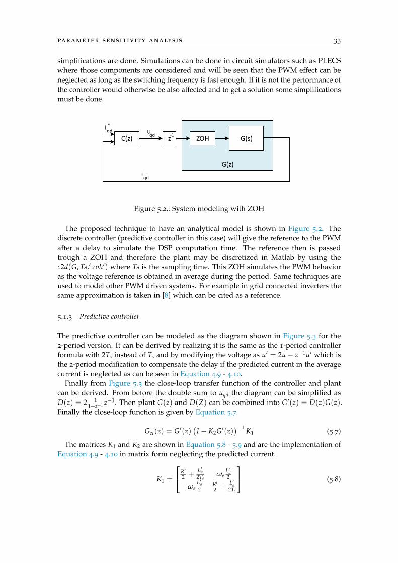
Figure 5.2.: System modeling with ZOH

The proposed technique to have an analytical model is shown in Figure 5.2. Thediscrete controller (predictive controller in this case) will give the reference to the PWMafter a delay to simulate the DSP computation time. The reference then is passedtrough a ZOH and therefore the plant may be discretized in Matlab by using thec2d(G, Ts,′ zoh′) where Ts is the sampling time. This ZOH simulates the PWM behavioras the voltage reference is obtained in average during the period. Same techniques areused to model other PWM driven systems. For example in grid connected inverters thesame approximation is taken in [8] which can be cited as a reference.

5.1.3 Predictive controller

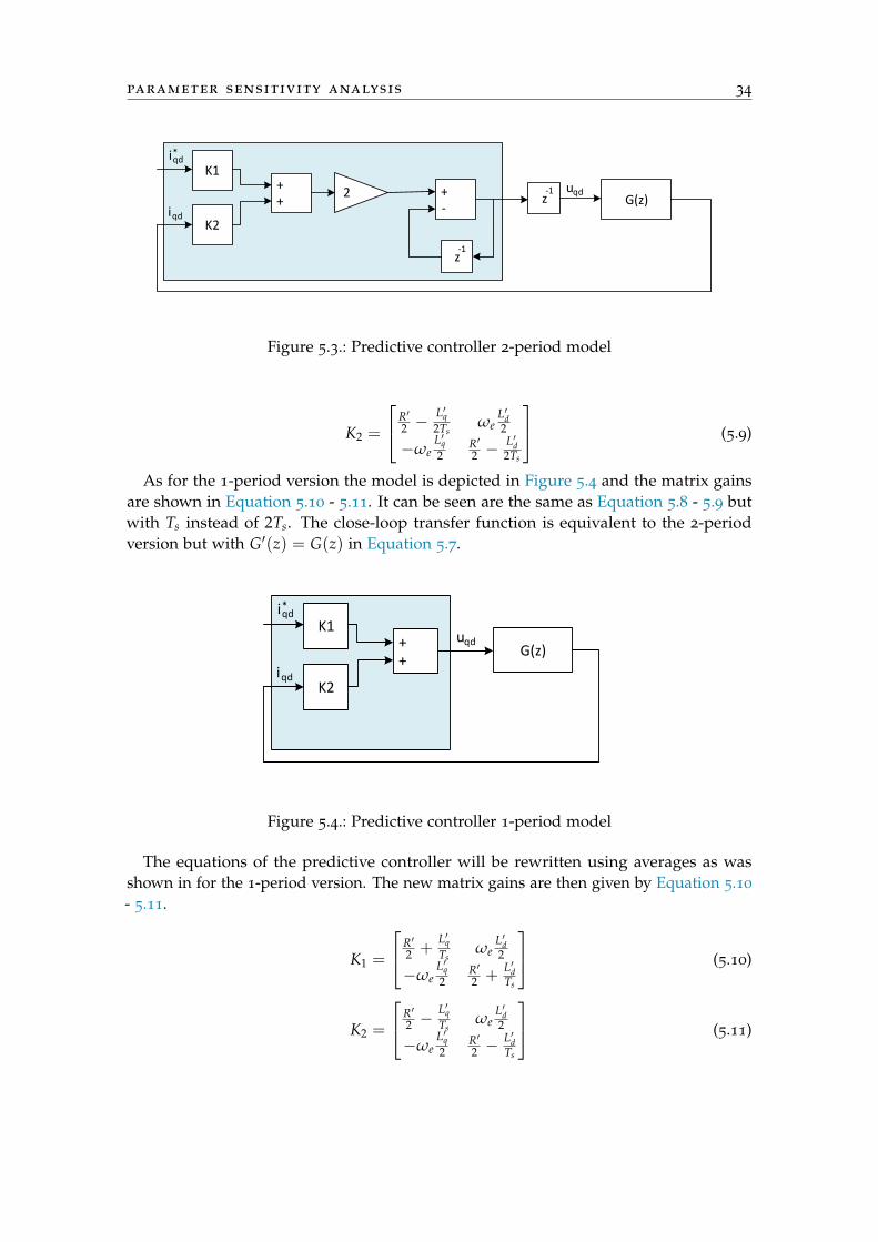
The predictive controller can be modeled as the diagram shown in Figure 5.3 for the2-period version. It can be derived by realizing it is the same as the 1-period controllerformula with 2Ts instead of Ts and by modifying the voltage as u′ = 2u− z−1u′ which isthe 2-period modification to compensate the delay if the predicted current in the averagecurrent is neglected as can be seen in Equation 4.9 - 4.10.

Finally from Figure 5.3 the close-loop transfer function of the controller and plantcan be derived. From before the double sum to uqd the diagram can be simplified asD(z) = 2 1

1+z−1 z−1. Then plant G(z) and D(Z) can be combined into G′(z) = D(z)G(z).Finally the close-loop function is given by Equation 5.7.

Gcl(z) = G′(z)(

I − K2G′(z))−1 K1 (5.7)

The matrices K1 and K2 are shown in Equation 5.8 - 5.9 and are the implementation ofEquation 4.9 - 4.10 in matrix form neglecting the predicted current.

K1 =

R′2 +

L′q2Ts

ωeL′d2

−ωeL′q2

R′2 +

L′d2Ts

(5.8)


z

K1

K2

++

+-

2 -1

z-1

iqd*

iqdG(z)

uqd

Figure 5.3.: Predictive controller 2-period model

K2 =

R′2 −

L′q2Ts

ωeL′d2

−ωeL′q2

R′2 −

L′d2Ts

(5.9)

As for the 1-period version the model is depicted in Figure 5.4 and the matrix gainsare shown in Equation 5.10 - 5.11. It can be seen are the same as Equation 5.8 - 5.9 butwith Ts instead of 2Ts. The close-loop transfer function is equivalent to the 2-periodversion but with G′(z) = G(z) in Equation 5.7.

K1

K2

++

iqd*

iqd

G(z)uqd

Figure 5.4.: Predictive controller 1-period model

The equations of the predictive controller will be rewritten using averages as wasshown in for the 1-period version. The new matrix gains are then given by Equation 5.10

- 5.11.

K1 =

R′2 +

L′qTs

ωeL′d2

−ωeL′q2

R′2 +

L′dTs

(5.10)

K2 =

R′2 −

L′qTs

ωeL′d2

−ωeL′q2

R′2 −

L′dTs

(5.11)


5.2 stability

The stability of the controller can be assessed by modifying each system parameterindependently (denoted without an apostrophe) and seeing the limits after where thesystem becomes unstable as the controller is not updating the parameters (denoted withan apostrophe). A simple way to represent the stability would be to perform a DC sweepin each system parameter and plot the poles position (of each element in the matrixGcl(z)) in a pole map. If all the poles are inside the unit circle the system is stable. Tosee the data better another graph can be added where the maximum absolute pole valueis plot vs the parameter change proportion. As long as this value is kept below 1 thesystem is stable.

The system stability is dependent of the speed and sampling time. Another setof graphs could be done where those variables are also modified to see the effect inthe system stability. However the result of testing at different speeds and switchingfrequencies showed almost no changes in the limits and is omitted for visibility of thepole map.

5.2.1 Resistor stability

The two graphs proposed are shown for the resistor in Figure 5.5 for both controllerswhere the controller parameters are set to the system’s except for the resistor of whichthe proportion of the system value over the controller (R/R′) is changed from −1 to 5.

-1 -0.5 0 0.5 1-1

-0.5

0

0.5

1

0.90.80.70.60.50.40.30.20.1

1π/T0.9π/T

0.8π/T0.7π/T

0.6π/T0.5π/T0.4π/T0.3π/T

0.2π/T

0.1π/T

1π/T0.9π/T

0.8π/T0.7π/T

0.6π/T0.5π/T0.4π/T0.3π/T

0.2π/T

0.1π/T

Pole map 2-period

R/R'-2 0 2 4 6

max

(abs

(z))

0.85

0.9

0.95

1

1.05Worst pole 2-period

-1 -0.5 0 0.5 1-1

-0.5

0

0.5

1

0.90.80.70.60.50.40.30.20.1

1π/T0.9π/T

0.8π/T0.7π/T

0.6π/T0.5π/T0.4π/T0.3π/T

0.2π/T

0.1π/T

1π/T0.9π/T

0.8π/T0.7π/T

0.6π/T0.5π/T0.4π/T0.3π/T

0.2π/T

0.1π/T

Pole map 1-period

R/R'-2 0 2 4 6

max

(abs

(z))

0.85

0.9

0.95

1


Figure 5.5.: Resistor error effect in stability in ZOH model


The blue values represent reductions in R and the red ones increments. It can be seenon the left the movement of all the system poles over the change in the ratio R/R′. Thestart is the green dot (R = R′). For simple results the worst pole location is shown in theright graph where the limit of stability is found at 0.

Even though the real resistor cannot be negative it is interesting to see there is alower limit at 0 for which the system becomes unstable. This limit can be verified inthe analytical model without PWM. There is no upper limit, therefore the results of theanalysis with a ZOH predict that the resistor alone cannot make the system unstableunless negative (which is not physically possible) and offer perspectives regarding thefact that this element may not play a big role in stability. It is also interesting to note thatthe real resistor will increase in value due to temperature and the graph of the right ofFigure 5.5 shows that as R is increased the system becomes more stable so it is expectedthat the resistor does not play a role in stability.

5.2.2 Lq stability

The graph for the analysis done in Lq where the system value is changed over thecontroller constant value L′q is shown in Figure 5.6. As it happened with the resistorthere are also zeros placed at almost the same position of the poles and zeros are omittedin the graph for readability as poles set the stability.

-1 -0.5 0 0.5 1-1

-0.5

0

0.5

1

0.90.80.70.60.50.40.30.20.1

1π/T0.9π/T

0.8π/T

0.7π/T0.6π/T0.5π/T0.4π/T

0.3π/T

0.2π/T

0.1π/T

1π/T0.9π/T

0.8π/T

0.7π/T0.6π/T0.5π/T0.4π/T

0.3π/T

0.2π/T

0.1π/T

Pole map 2-period

Lq/L

q'

0 1 2 3 4

max

(abs

(z))

0.9

1

1.1

1.2

1.3

1.4


-1 -0.5 0 0.5 1-1

-0.5

0

0.5

1

0.90.80.70.60.50.40.30.20.1

1π/T0.9π/T

0.8π/T

0.7π/T0.6π/T0.5π/T0.4π/T

0.3π/T

0.2π/T

0.1π/T

1π/T0.9π/T

0.8π/T

0.7π/T0.6π/T0.5π/T0.4π/T

0.3π/T

0.2π/T

0.1π/T

Pole map 1-period

Lq/L

q'

0 1 2 3 4

max

(abs

(z))

0.5

1

1.5

2


Figure 5.6.: Lq error effect in stability in ZOH model


It can be seen on the graph on the right that the limit of stability is almost the one forwhen the real inductor drops to half the one used in the controller. This limit makessense as later in Equation 5.19 is approximated the overshoot as a function of L/L′ and itis found that when L = 0.5L′ the overshoot is 100% so if the real inductor L drops morethan that the overshoot is bigger than 100% so it would tend to amplify any error.

5.2.3 Ld stability

The graph for the analysis done in Ld where the system value is changed over thecontroller constant value L′d is shown in Figure 5.7.

-1 -0.5 0 0.5 1-1

-0.5

0

0.5

1

0.90.80.70.60.50.40.30.20.1

1π/T0.9π/T

0.8π/T

0.7π/T0.6π/T0.5π/T0.4π/T

0.3π/T

0.2π/T

0.1π/T

1π/T0.9π/T

0.8π/T

0.7π/T0.6π/T0.5π/T0.4π/T

0.3π/T

0.2π/T

0.1π/T

Pole map 2-period

Ld/L

d'

0 1 2 3 4

max

(abs

(z))

0.9

1

1.1

1.2

1.3

1.4


-1 -0.5 0 0.5 1-1

-0.5

0

0.5

1

0.90.80.70.60.50.40.30.20.1

1π/T0.9π/T

0.8π/T

0.7π/T0.6π/T0.5π/T0.4π/T

0.3π/T

0.2π/T

0.1π/T

1π/T0.9π/T

0.8π/T

0.7π/T0.6π/T0.5π/T0.4π/T

0.3π/T

0.2π/T

0.1π/T

Pole map 1-period

Ld/L

d'

0 1 2 3 4

max

(abs

(z))

0.5

1

1.5

2


Figure 5.7.: Ld error effect in stability in ZOH model

As expected the results seem to be the same as for Lq. The limit is the same for the1-period version.

5.2.4 Flux stability

The flux has been left out of the equations for simplicity as it can be seen as DC term inthe voltage command from a mathematical point of view and therefore it is treated as aperturbation. The flux could be considered by adding the term

(λ′mpm − λmpm

)ωe to the

voltage q axes. This is represented in Figure 5.8.


PredictiveController ++

i qd*

Gpmsm(z)

λmpm-λ mpm0

ωe

i qd

uqd*

Figure 5.8.: Flux estimation error perturbance

Since the system is linear the response of the system can be seen as the combination ofthe controller voltage plus the flux difference due to errors in the parameter estimationof the flux. If the controller+system is stable the flux then cannot make the responseunstable as it is a constant DC term added to the q voltage.

5.2.5 Conclusion

From the results presented it can be seen only inductors play a role in stability and makethe system unstable when dropped to half. This value changes slightly with speed andTs but it is very close to 0.5 always. The resistor on the other hand only makes the systemunstable if negative which could be considered a theoretical limit.

5.2.6 Simulation results

The limits obtained analytically with the ZOH approximation can be validated in simula-tion where the PWM at fs = 3000Hz is no longer neglected. To sum up the results thefollowing was found out:

• A negative resistor makes the system unstable.

• A drop in any inductor by half makes the system unstable.

• The flux does not affect stability if the speed is considered to change slowlycompared with the current.

Resistor limits

It has not been possible to simulate a case in which the resistor makes the systemunstable with the predictive controller.


Inductor stability

With the 2-period controller the system becomes unstable in simulations when anyinductor drops to around 0.47 times its initial value. This value is very close to the oneestimated of 0.5.

Flux stability

As predicted it has been impossible to make the system unstable by modifying the flux.Different values from up to ±10 times have been tried. What has been found is that aslong as the speed is not changing since its effect is a DC perturbation it does not affectthe transient. If the speed changes considerably it can also affect the transient since it isno longer a constant DC perturbation but since changes are slow it does not play a bigrole in the transient either.

Conclusion

Based on the simulation results it can be concluded that the only elements that seem toplay a role in the stability are the inductors. As long as the speed is not changing theflux error is only a DC offset. Both resistor and flux cannot make the system unstablebut they can affect the transient response (the flux only when the speed is changingconsiderably) and the resistor at low load/speed conditions when it has an importantweight in the voltage equation.

5.2.7 Experimental results

The limits of stability calculated analytically and tested under simulations can be vali-dated experimentally. It has been found in simulations that the limits estimated analyti-cally coincide with the ones in simulations except for the resistor which seems to not beable to induce instabilities contrary with the results obtained from the root-locus plot.Since the main difference between the analytical model and the simulations is the PWMit is expected for this to be the reason of discrepancies and therefore in the experimentalresults this is expected to happen:

• Resistor will not play a role in stability.

• A drop in any inductor by half makes the system unstable.

• The flux does not affect stability if the speed is considered to change slowlycompared with the current.

To validate all those claims the following tests are proposed. The machine is setrunning and the parameters used in the controlled are changed to ensure the sameproportions found in the limits analytically. Then a step in id will be commanded andthe response recorded. For a stable system the controller will be able to settle to a valueand if the system becomes unstable it will start to oscillate with bigger oscillations eachperiod which will trigger the protections and shut down the system.


5.2.8 Resistor limits

Different values have been tested from −2R to 2R and the system is always stable. Theonly change is a steady-state error and at low speeds the transient is also affected.

5.2.9 Inductor limits

As the value of Ld used in the controller is increased it is seen that around 4.4mH thesystem starts presenting big oscillations as depicted in Figure 5.9.

Time [s]10 15 20 25

i d [A

]

-6

-4

-2

0

2

4

6

8

10

12id current response for L

d' = [L

d,2L

d]

id*

id

Period0 5 10 15 20

i d

-6

-4

-2

0

2

4

6

8

10

12Zoomed in view

id*

id

Ld set to double

Figure 5.9.: Response on id as controller inductor is doubled

Moreover a high pitch noise is heard which makes sense as based in the currentresponse every period the current changes almost 10A so a noise of 2 fsw is expected tobe heard.

5.2.10 Flux limits

Different values have been tested from −2λmpm to 2λmpm and the system stability hasnot been compromised.

5.3 steady-state errors

In this section the effect of errors in the parameters will be considered to come upwith an idea of how they affect the steady-state errors. The controller and machineequations will be rewritten for the steady-state case by removing the differential termswhen appropiate.


5.3.1 System equations

In steady-state the current can be considered constant within periods and therefore, onaverage the differential terms do not appear in the voltage on the system. The currentwill change due to the PWM nature but the average will still be close to the value at thebeggining and end of the period (which will be the same).

Under this considerations the steady-state machine equations can be rewritten inmatrix form as Equation 5.12.[

uq

ud

]= MSS

[iq

id

]+ λ =

[R ωeLd

−ωeLq R

] [iq

id

]+ ωe

[λmpm

0

](5.12)

5.3.2 Controller equations

In steady-state the differential terms of the controller will be zero only if there is nosteady-state error. However, if there is some steady-state error this difference will still befed to the differential terms and therefore they cannot be removed. There will be twovariables in the controller side, the reference currents and the actual value.

Recalling from before K1 was defined in Equation 5.10 and K2 in Equation 5.11 for the1-period controller and the controller equations are then given by Equation 5.13 wherethe last term will be denoted simply as λ′.[

uq

ud

]′= K1

[iq

id

]∗+ K2

[iq

id

]+ ωe

[λ′mpm

0

](5.13)

In this case the results change between 1-period and 2-period version due to thedifferent gains used. The derivation for the 2-period version is the same but noting thefollowing changes. In K1 and K2, the term Ts should be changed into 2Ts. On the otherhand in K1 the term 1/2 is changed into 2/3 and the term 1/2 into 1/3 in K2. This isbecause the predictive controller estimates the current reference in the average terms,which without saturation will be the same as the reference. In steady-state the voltagecommand will also be the same in every period so uk+uk+1

2 = u = f (i∗qd, iqd, ωe, 2Ts).

5.3.3 Equations of steady-state errors

With the models defined in the two previous subsections the steady-state errors canbe calculated by solving the currents as a function of the reference and the machineparameters and working condition by imposing that the voltage applied in controllerand machine must be the same. The solution for iqd is then found in Equation 5.14.

i′qd = (MSS − K2)−1(

K1i∗qd + λ′ − λ)

(5.14)

And the error then can be defined as εqd = i′qd − i∗qd. As there is a matrix inversionwith all the elements defined it can be inferred that the analytical solution will not besimple. Therefore to interpret the results the formulas derived will be used to plot theerrors in different conditions.


5.3.4 Results

The effect of changing individually any parameter is shown in Figure 5.10 for a referenceof i∗q = 15 and i∗d = 3 as setting i∗d = 0 removes any error due to Ld. The graphs are donealso for 4 different speeds of 0, 33, 67, 100Hz with Ts = 3000Hz and the result plotted isthe absolute error for the q and d current given by iqd − i∗qd.

R/R'1 1.5 2 2.5 3

Cur

rent

err

or [A

]

0

0.2

0.4

0.6

0.8

Lq/L

q'

0.5 0.6 0.7 0.8 0.9 1C

urre

nt e

rror

[A]

0

0.5

1

1.5

Ld/L

d'

0.5 0.6 0.7 0.8 0.9 1

Cur

rent

err

or [A

]

-0.3

-0.2

-0.1

0

f = 0 (q)f = 33 (q)f = 67 (q)f = 100 (q)f = 0 (d)f = 33 (d)f = 67 (d)f = 100 (d)

Lmpm

/Lmpm

'0.8 1 1.2

Cur

rent

err

or [A

]

-2

0

2

Figure 5.10.: Steady-state error due to parameter error one parameter at a time

As it seems logical the absolute error is bigger in the q axes as the reference is set 5times bigger. It can be seen that Ld does not play a big role as long as id is kept low.Theoretically if i∗d = 0 errors in Ld do not affect the steady-state errors. However thetransient phenomena will be affected and as was proved before if Ld dropped more thanhalf the system would become unstable.

5.3.5 Steady-state errors approximation

It can be seen in Figure 5.10 that even though the equation solutions are not linear dueto the matrix inversion the error produced when only one parameter is changed at atime looks linear. This suggests that to characterize the effect of any combination ofparameters at a time and working condition (load, speed, more than one parameterchange) the equations obtained may be approximated with Taylor expansion in the 4

machine parameters and this way they will be easier to interpret as there are 8 parametersinto play and a plot with every combination is not possible.

Derivations are omitted here and attached in Section B.2 where it is also shown inFigure B.3 that the approximation tends to produce an error in the error of less than


5% so it can be considered adequate and used to infer the relations between states andparameters in the global error. The result of the approximation is that the error can beestimated as Equation 5.15 where Kss is given by Equation 5.16.

e(iqd) = iqd − i∗qd ≈ Kss

∆R∆Lq

∆Ld∆λmpm

(5.15)

Kss =

− TsLq

i∗q − Ts2 i∗q ωe

2

2 Lq− Ts i∗d ωe

Lq− Ts ωe

Lq

− TsLd

i∗dTs i∗q ωe

Ld− Ts

2 i∗d ωe2

2 Ld− Ts

2 ωe2

2 Ld

(5.16)

Difference between 1 and 2-period controller consist in the constants that multiply thecoefficients of the Taylor approximation (for example 1/2 may become 2/3 and so on) sothe relations observed inferred from Taylor (what variables affect what) are the same.From the Taylor approximation the effect of each parameter and state in the global errorcan be understood in simple terms and will be discussed in the following sections.

Parameter error analysis

Since the full taylor approximation of first order has been validated to produce an errormoderately low of typically less than 5% it may be considered valid to use as a way tostudy the effect of each parameter variation in the steady-state error. Moreover if thespeed is kept below half the nominal Equation B.16 can be used. At higher speeds thenit may be modified by multiplying it by d2

d2+d5. This comes from the approximation taken

in Equation B.13.The advantage of this approximation is that it shows that the effect of each parameter to

the error in each axis is independent of each other and is only function of two parametersonly: the speed, and the current reference in one axis only. Because of this a plot for eachparameter can be developed and the total error can be approximated as the sum of eachparameter contribution to the error in each plot. From the taylor approximation of whichformulas were shown in Equation 5.16 the following dependencies in Figure 5.11 betweenerrors and system states can be inferred with a good approximation. The diagram canbe interpreted as follows. An error in Lq for example produces an error in both the qand d current, e(iq) and e(id) as a function of i∗q . The reference i∗d does not influence theerror significantly. The errors are speed-dependent (yellow). The resistor for exampleproduces an error on each axis as function of both i∗q and i∗d , being i∗q the command thataffects the error in q and i∗d the error in d. Because of the green color the speed does notplay a big role. Finally the flux is current independent and produces a constant error thatis greatly influenced by the speed (red). The approximated errors can then be calculatedapplying superposition to Figure 5.12 or Figure 5.13 for the system parameters obtained.

If the switching frequency also wants to be taken into account then the speed used tolook in the plot may be modified into ωeT′s/Ts as the speed is always multiplied by Ts

in the taylor approximation except the resistor where the current should be modifiedas iT′s/Ts. Results are depicted in Figure 5.12 for the 1-period deadbeat version usingthe relations inferred from the Taylor approximation but the exact error as given by


R Lq Ld

iq* id*

e(iq) e(id)

Lmpm

Figure 5.11.: Error dependencies between system parameters and states

Equation 5.14. The same calculations can be redone for the 2-period version and theresults are depicted in Figure 5.13 since the errors change considerably.

The graphs can be interpreted as follows. The error in the y-axis is the absolute errorproduced either in the q (blue) or d axis (red) current due to a change of +10% in theparameter. The error in this case was defined as iqd − i∗qd so for example a positive valuemeans the current generated by the controller will be bigger than the reference. Since theformulas are approximately linear to see the effect of any other change the proportionwhich respect to the initial parameter may be multiplied. For example to see the effect ofa 20% drop in Lq the value obtained from the graph may be multiplied by −0.2/0.1 asthe values are done for +10% change.

The error is plotted as a function of current reference and speed as those are the onlytwo factors that affect it within each parameter without making a significant error. Thechange due to current is linear and due to speed is linear in some parameters only. Thespeed is varied from 0 to rated speed. The brighter the color the bigger the speed whichgoes from 0 to rated 2π300.

To validate the results the parameters in the machine may be changed under sim-ulations and the error for a given state estimated with Figure 5.13 since the 2-periodcontroller is implemented in simulations. Let for example R = 1.3R0, Lq = 0.8Lq0, Ld =

0.75Ld0, Lmpm = 0.9Lmpm0 and the states i∗q = 10, i∗d = 6, ωe = 2π100 with fs = 5Khz. The error can be estimated from Figure 5.13 and the procedure is depictedin Table 5.1. The values can be read directly from the graph and multiplied by0.3/0.1,−0.2/0.1,−0.25/0.1,−0.1/0.1 for each parameter as the graph is made forchanges of +10%. To gain precision the values are actually calculated from Equa-tion 5.14 but maintaining the approximations taken. For example in Lq the error due to


iq* (blue) / i

d* (red) [A]

-20 -10 0 10 20

Cur

rent

err

or [A

]

-0.05

0

0.05

R ss-error

iq* [A]

-20 -10 0 10 20

Cur

rent

err

or [A

]

-0.5

0

0.5

Lq ss-error

id* [A]

-20 -10 0 10 20

Cur

rent

err

or [A

]

-0.5

0

0.5

Ld ss-error

Current independent [A]-20 -10 0 10 20

Cur

rent

err

or [A

]

-2

-1.5

-1

-0.5

0L

mpm ss-error

Figure 5.12.: Error in iqd due to each parameter, i∗qd, and speed for 1-period deadbeatcontroller for fs = 5 kHz

iq* (blue) / i

d* (red) [A]

-20 -10 0 10 20

Cur

rent

err

or [A

]

-0.1

-0.05

0

0.05

0.1

R ss-error

iq* [A]

-20 -10 0 10 20

Cur

rent

err

or [A

]

-1

0

1

Lq ss-error

id* [A]

-20 -10 0 10 20

Cur

rent

err

or [A

]

-1

-0.5

0

0.5

1

Ld ss-error

Current independent [A]-20 -10 0 10 20

Cur

rent

err

or [A

]

-3

-2

-1

0L

mpm ss-error

Figure 5.13.: Error in iqd due to each parameter, i∗qd, and speed for 2-period deadbeatcontroller for fs = 5 kHz


i∗d is removed and it will also calculate the error for a 10% positive change in Lq and thenmultiply the result by −0.2/0.1.

Parameter e(iq) e(id)

R −0.13 −0.08Lq 0.08 −0.50Ld 0.34 0.06

λmpm 1.35 0.23Total error 1.60 −0.30

Table 5.1.: Random parameters variation for Taylor approximation validation

The errors have been estimated with the approximations presented. Now the machineis set at the desired speed and the inertia is set high so the speed does not change duringthe simulation. The references are set as commented and the parameters in the machinemodified according to the numbers set. The current response is shown in Figure 5.14.The error may be calculated then from Figure 5.14 as e(iq) = 11.6 − 10 = 1.60 ande(id) = 5.6− 6 = −0.40. It can be seen good concordance between the approximation(−1.60, 0.30) and the simulation. If the formula in Equation 5.14 is used directly insteadthe error would be estimated as 1.58 and −0.40 showing that Equation 5.14 is valid andthe origin of the errors are attributed to the approximations taken but it can be seenthat they are still kept low and can be used to infer good intuitions about how eachparameter and system state affect the steady-state error.

Time [s]0 0.02 0.04 0.06 0.08 0.1

Cur

rent

[A]

-10

-5

0

5

10

15

20iq

iq*

iq

Time [s]0 0.02 0.04 0.06 0.08 0.1

Cur

rent

[A]

-2

-1

0

1

2

3

4

5

6

7

8id

id*

id

X: 0.1Y: 5.602X: 0.1

Y: 11.6

Figure 5.14.: Error in iqd with the states set in simulation

Conclusion

The effect of each parameter in the steady-state error can be calculated accurately withEquation 5.14. Due to the dependency of so many parameters an approximation havebeen taken with relatively low errors and the dependency between parameters is shown


in Figure 5.11. The errors can be estimated with good precission applying superpositionwith the graphs from Figure 5.12 - 5.13 which show how each parameter and state affectthe global steady-state error. Both current and speed can change the steady-state errorsdramatically and the worst case is always with the biggest of the two. The error inthe resistor estimate plays a small role in the steady-state error when compared withthe other three parameters. If i∗d = 0 then any error in Ld will not produce an error inany current. Switching frequency also plays an important role similar to speed in thesteady-state errors since the effect of a different frequency f ′s is equivalent as the errorrunning the machine at ω′e ≈ ωe

fsf ′s

in all parameters but the resistor which on the otherhand tends to produce small errors.

5.4 transient response

The effect of the change in any machine parameter in the performance of the controlleris studied in this section.

The resistor effect in the transient is neglected as it only affects at lower loads andspeeds since its voltage contribution is usually low compared to the inductors and fluxparts. On the other hand from Figure 5.8 it can be seen that errors in the flux linkagecan be understood as a DC perturbation to the voltage command since changes in thespeed are slow compared to changes in the current. This does not necessarily meansthat they will not affect the transient as the controller will work differently when tryingto compensate them (the differential terms for example will never be zero as therewill always be an error under changes in the flux) it was seen under simulations andexperiments that the effect to the transient when it is wrongly estimated is usually small.

For this reason the transient response will only take into account the effect of changesin the inductors as they are the main contributors to it. Later the DC claim will bevalidated under some approximations.

5.4.1 Overshoot

If the resistor and flux terms are neglected in the transient they can be removed fromthe system and controller equations as they are considered compensated. Then, thefollowing relations can be derived in Equation 5.17 - 5.18 to estimate what happens whena step is sent to the controller in the 1-period version.

Lq

Ts∆q + ωeLd < id >=

L′qTs

∆q∗ + ωeL′d < id >∗ (5.17)

Ld

Ts∆d−ωeLq < iq >=

L′dTs

∆d∗ −ωeL′q < iq >∗ (5.18)

The inductor Lx (where x is any axis, q or d) is the real inductor in the machine butthe controller has the estimate L′x. The value of < ix >∗= i∗x+ix

2 is the average current inthe period as estimated by the controller where i∗x is the current command and ix thecurrent at the beginning of the period. The real one will be < ix >= i′x+ix

2 where i′x is theactual current at the end of the period. The value of ∆i∗x is the commanded change given


by i∗x − ix that can be understood as the step in the x axis. The actual step however willbe ∆ix = i′x − ix.

At low speeds the coupling terms are not significant either in comparison with thedifferential part and may also be neglected and since then the steady-state error will besmall as is the speed then the overshoot can be approximated as Equation 5.19. Underthose approximations the overshoot in the 2-period version must be the same also as Ts isremoved from the equations. Negative values indicate the system is over-damped. Thisapproximation is at first sight only valid when steady-state errors are small but gives anidea about the evolution of the overshoot. When the coupling terms are considered theywill modify the steady-state error and also the transient response making the overshootspeed dependent also. Moreover since the equations are coupled errors in Lq will affectthe overshoot in Ld and the other way around. However it has been seen that as long asthe errors are constant (for example flux errors, or the current reference is set constant inthe other axis and does barely change so introduces a constant error) then the equationEquation 5.19 seems to be quite accurate understanding ∆x∗ as yss− y0 and ∆x as yp− y0

based on simulations. Those variables are shown in Figure 5.16. A simple proof of whyEquation 5.19 works for cases with constant steady-state errors and dc perturbations isconducted in Section B.3.

ov = Φ ≈ ∆x∆x∗− 1 =

L′xLx− 1 (5.19)

To validate the claims as only 2 parameters are the main responsible of the overshoot(inductor error and speed) then the following procedure can be done. A model in PLECScan be developed where those parameters are varied and a step in the q axis is given andthe overshoot calculated from a script. It has been seen that the overshoot is not affectedin great value by errors in the other parameters, current references or previous currentstates in d, and step size in q based on simulations as they produce dc perturbations.Same happens for d. As predicted the overshoot is speed dependent but the relation isnot that important either. The speed ωe and the coefficient between the real inductorand controller, Lq/L′q, may be varied in the model run from a Matlab script trough twoloops. The results are depicted in Figure 5.15. Additionally, in red the approximationfrom Equation 5.19 has been plotted.

The speeds used have been 2π[0, 75, 150, 225, 300] where 2π300 is the rated speed. Itcan be seen that the speed does not play such a significant role in the overshoot. Theerrors at high speeds when the parameters are correct are due to the coupling effectsinfluencing the results due to the discretization of the controller and having a continuousplant. An step in one axis changes the other current slightly which is not predicted bythe controller. This is due to the average approximation used which is worse as the speedincreases. Increasing fs removes any coupling effect. Therefore this current that appearsin the other axis that is not accounted for modifies slightly the initial step making a smallovershoot.

It can also be seen that the approximation from Equation 5.19 is quite accurateand as expected tends to be better as the error in the inductor is increased and thespeed is decreased as that increases the weight of the differential term in the overshootcontribution.


Lq/L

q'

0.6 0.65 0.7 0.75 0.8 0.85 0.9 0.95 1

Ove

rsho

ot

0

0.1

0.2

0.3

0.4

0.5

0.6

0.7

Speed

Speed

Figure 5.15.: Overshoot in iq as a function of inductor error and speed

5.4.2 Settling time

The settling time defined as the time it takes for a signal to stabilize within a toleranceband can be estimated under some approximations in the 1-period controller. Theovershoot, Φ, is mostly function of the speed ωe and more importantly the relation L/L′.Therefore, since the 1-period deadbeat controller has no delays there is no reason tothink the proportion Φ will change in any period after the first step. Then it must betrue that the response of the system must follow with good approximation Figure 5.16.

When a step is given the signal will go to (1+ Φ)s where s is the real step of the signalas given by s = yss − y0 and Φ the real overshoot as yp−yss

yss−y0. This means the error with

respect to the steady-state value is given by (1 + Φ)s− 1 = Φs. In the next period thecontroller will try to compensate and the signal will go below the steady-state value aproportion lower than the original overshoot. In absolute value since the step now is Φsthen the signal will go to (1 + Φ)(Φs) so the signal will have now an error with respectto Φs as given by (1 + Φ)(Φs)−Φs = Φ2s. This may be generalized for any period k asΦn × (−1)(2k+2)s. The term −12k+2 may be removed as it only gives information aboutthe side of the error which is not needed for the settling time. On the other hand it seemssensible to use settling time in an relative sense, therefore the value may be scaled by theoriginal step size s. The final formula is then simply Φn. The settling time then may becalculated as the time it takes to reach a relative tolerance of p. The number of periods ittakes to settle, nss, may then be solved from Φnss = p and it is given by Equation 5.20.The value of Φ may be estimated from Equation 5.19 or taken from Figure 5.15. If thereal inductor increases and there is an over damping response then Φ may be replaced


yss

y0

ypΦs

s

k = 1

k = 0

k = 2

k = 3

Φs 2

3Φs

Figure 5.16.: Settling time with approximation taken for 1-period controller

by −Φ in Equation 5.20 as the same behavior as with overshoot is expected. Therefore togeneralize Φ may be replaced by abs(Φ) in Equation 5.20 to account for both cases.

nss(1) = 1 +log plog Φ

(5.20)

As a way to validate the simplifications taken a step response in the q axis at ωe = 2π50and with Lq/L′q = 0.7 is performed and the results are depicted in Figure 5.17. It can beseen great concordance with the approximation from Figure 5.16.

For the 2-period controller since there is a delay present the approximation of constantovershoot and Φn is not valid anymore as the previous state influences the next overshoot.

The response to a step in q in both axis for Lq/L′q = 0.7 and two speeds, ωe = 2π20and ωe = 2π200 is depicted in Figure 5.18. The error in the inductor yields an overshootfollowing the same derivations as in 1-period.

It can be seen from Figure 5.18 at low speeds the oscillations tend to be at 2Ts while athigher speeds they are faster at Ts. The settling time takes also more duration that in the1-period version due to the delay in the command. As a rule of thumb from simulationresults the algorithm seems twice as slow as the 1-period version, so the settling timemay be approximated as nss(2− period) ≈ 2nss(1− period) where nss(1− period) wasapproximated in Equation 5.20. So the settling time for the 2-period version may beapproximated as Equation 5.21.

nss(2) = 2(

1 +log p

log abs(Φ)

)(5.21)


Period0 2 4 6 8 10 12 14 16 18 20

i q [

A]

-2

0

2

4

6

8

10

12

14

iq

*

iq

Φ(0) = (14.33-10.14)/10.14 -1 = 0.4132

Φ(1) = (10.14-8.423)/10.14 -1 = 0.16930.1693 0.4132^2 = 0.17

Φ(2) = (10.85-10.14)/10.14 -1 = 0.070.07 0.4132^3 = 0.0705

Figure 5.17.: Settling time with approximation taken for 1-period controller for Lq/L′q =0.7 and ωe = 2π50

Period0 10 20 30

i q [A

]

0

5

10

15fe = 20

iq*

iq

Period0 10 20 30

i d[A

]

4

4.5

5

5.5

6fe = 20

id*

id

Period0 10 20 30

i q [A

]

0

5

10

15fe = 200

iq*

iq

Period0 10 20 30

i d[A

]

2

4

6

8fe = 200

id*

id

Figure 5.18.: Step response for 2-period controller for Lq/L′q = 0.7 and ωe = 2π20 andωe = 2π200


Finally the settling time may be calculated from simulations with two nested for loopsvarying Lq/L′q and ωe. The model is set running for different combinations and thesettling time it is estimated as the time it takes for the signal to settle within 5% of thefinal value. The results are depicted in Figure 5.19 for the 1-period controller and inFigure 5.20 for the 2-period version. In dashed red the approximation from Equation 5.20

and Equation 5.21 is shown. It can be seen good concordance between the approximationand the simulation results.

Lq/L

q'

0.6 0.7 0.8 0.9 1 1.1 1.2 1.3 1.4 1.5

Set

tling

per

iods

for

5%

1

2

3

4

5

6

7

8

fe = 0

fe = 75

fe = 150

fe = 225

fe = 300

Estimated nss

Figure 5.19.: Settling time (5%) for different Lq/L′q and ωe at fs = 5 kHz for 1-periodcontroller

Lq/L

q'

0.6 0.7 0.8 0.9 1 1.1 1.2 1.3 1.4 1.5

Set

tling

per

iods

for

5%

2

4

6

8

10

12

14

16

fe = 0

fe = 75

fe = 150

fe = 225

fe = 300

Estimated nss

Figure 5.20.: Settling time (5%) for different Lq/L′q and ωe at fs = 5 kHz for 2-periodcontroller

5.4.3 Conclusion

The transient response evolution due to parameter errors in the estimates has beenstudied. The resistor effect is neglected due to the typically small contribution to thevoltage equations. It has been found that with good approximation the overshoot and


settling time is mostly function of only the inductor error as DC perturbations do notinfluence the overshoot greatly and settling time is dependent of overshoot mostly.

The speed also influences the overshoot and settling time and helps the transientresponse in certain conditions as evidenced by the graphs. Overshoot and settling timeare asymmetrical with respect to the inductor error as can be seen by the approximationin the formulas derived in and also in the simulation results presented. Increases inthe real inductors make the system slower and more robust and decreases also produceslower responses with oscillations. Both the settling time and overshoot/overdampingis more affected when the inductors drop. For example a drop of the inductor by halfproduces an overshoot of 100% and a marginally stable system but an increase of theinductor to double produces an initial error in the over-damping system of 50% and asettling time around 5 times slower than having no error.

6N O N - L I N E A R I T I E S C O M P E N S AT I O N

In this chapter different non-linearities that affect the converter are presented andcompensated as they affect the voltage command given by the controller and decreaseperformance and can make machine parameter estimations difficult at certain conditions.Each non-linearity is studied independently and at the end simulation and experimentalresults are presented. Apart from the main discrete method a resonant compensatorimplementation is also analyzed with experimental validation which provide goodresults at low speeds.

6.1 deadtime

The converter IGBTs need some time to commute from one state to another. This timehas some variations depending of the temperature and other factors. Because of thisanother time td bigger than those two is added to guaranty enough time for the currentto change paths. Each time the PWM pulse change it is delayed by td as explained in [9].

Vdc

Sup

Slowi > 0

i < 0

Figure 6.1.: Converter leg with the current paths

On this period of transition no pulses are given and the effect in the voltage changedepends on the current sign as can be seen in the circuit in Figure 6.1 for one leg for oneperiod of the triangular. If no pulses are given depending of the current sign it will flowone way or another inducing either vdc or 0. The effect in the other legs is the same andindependent.

The effect on the signals is shown in Figure 6.2. When the current is positive andno pulses are given the lower part will conduct as the current can flow trough the

54

non-linearities compensation 55

Td

Upper transistor switch

Sup

(Ideal)

Sup

(Real)

Td

Bottom transistor switch

Slow

(Ideal)

Slow

(Real)

Td+t

ONtOFF

Td+t

ONtOFF

Desired voltageV

leg(Ideal)

Vleg

(i>0)

Vleg

(i<0)

Figure 6.2.: Deadtime effect in the voltage command

bottom diode. After the delayed td and tON it will switch to the igbt that is commanded.Therefore there will be a voltage drop in the transition from down to top igbt. On thecontrary, when it switches from the lower igbt it will do so almost instantly at the timetOFF which induces a small voltage gain. When the current is negative something similarhappen. On the switch from the top part to the bottom it will be delayed by td and tONas the current can travel freely trough the top diode and the delay will be tOFF onlywhen it goes back to the positive state and thus induces a voltage gain.

Moreover the voltage drop in the components of the converter will produce morechanges in the voltage command. All those modifications can be predicted and compen-sated.

During the development of the compensator several simplifications will be donein order to be able to develop a compromise with simple analytical solutions andgood performance. The results of the simulations will show that the simplifications areadequate and the results of the experiments will evidence that the modeled non-linearitieshave been done correctly.

To compensate for this time delay td one can calculate the voltage difference that isproduced and add it directly to the reference. This can be done due to the linearity ofthe system and the independence of the time delays of the input as will be explained. Ifthe voltage drop given by the time delays was a function also of the reference then thevoltage drop could not be directly added to the reference and more calculations may bedone to get a better result.

On a fundamental level, the converter voltage (which respect to its neutral placed in thenegative side of udc) can be written as Equation 6.1 where the duty times can be rewrittenas Equation 6.2, that is the reference duty time d∗ coming from the modulator (which


receives the original voltage command from the controller) followed by the undesireddead time duty cycle dd. uan

ubnucn

= udc

da

dbdc

(6.1)

di = d∗i + dd (6.2)

Because dd is only a function of the current direction as explained before it is indepen-dent of the reference d∗ and therefore if d∗ is transformed in d∗ − dd the final result willnot have the deadtime. So to compensate the deadtime this dd can be calculated at anymoment and added directly to the duty cycle that is given to the PWM hardware. Thevalue of di is on average (−tON − td + tOFF)/Ts when ii > 0 and (tON + td − tOFF)/Ts

when ii < 0. The values of tON and tOFF will be neglected.To see the effect of the deadtime in dq as the control is done in this reference frame the

duty cycles can be transformed into Line-Line voltages in the converter and this to line-neutral machine voltages using Equation 2.6. For a balanced system, for a fundamentalperiod, the injected voltage vd is calculated and shown in Figure 6.3 for the values ofTable 6.1. For reference the distortion in phase-a voltage is also presented.

Name Value

udc(V) 325

fsw(Hz) 5000

td(µs) 4

Table 6.1.: Parameters for the deadtime voltages

This voltage can be transformed to dq0 and is shown on the right. It can be seen thatthe effect in q is a DC offset and a sinusoidal and in d there is not such offset but rathera triangular shape.

0 0.005 0.01 0.015 0.02-10

-5

0

5

10

0 0.005 0.01 0.015 0.02-5

0

5

10

uq

ud

Figure 6.3.: Voltage injected due to the deadtime in abc for one phase and dq respectively

If this voltage distorsion is then injected as duty cycles to the PWM with reversesign the deadtime can be considered to be compensated. Therefore the voltage of thecontroller is still being used directly in the equations to predict parameters. The flowchartdescribing the algorithm for one leg is shown in Figure 6.4.


Ij(k+1) Ij(k+2)

>0

Td/Ts

<0

-Td/Ts

Leg j

Predicted currentsfor when v* is

applied

To pwm(delayed ifneeded)

DeadtimeCompensaton

algorithm

+ +

Δdj

Figure 6.4.: Steps performed in one leg to compensate deadtime

6.2 snubber compensation

Some converters have snubbers in parallel with the diodes to try to minimize the effect ofthe dead-time in the voltage change. As explained in [10] the snubbers may be modeledas just capacitors. Under this assumption a compensator that has into consideration thechange in the voltage due to these capacitors can be added to the dead-time.

The effect in the signals is shown in Figure 6.5. When the current is positive and needsto change from the top to the bottom part it is delayed td and on this case due to thesnubbers it will have two paths to follow trough both capacitors. The capacitor on thetop is discharged as the top part was conducting and the voltage on it is the same as inthe transistor that can be neglected. On the bottom, on the other hand the capacitor ischarged to Vdc as when the top transistor was on it was directly connected to the source.In this transition, half the current will go trough the top capacitor and half trough thebottom as both capacitors must discharge at the same rate and are considered to havethe same capacitance. Therefore it can be seen that the voltage in the terminal will notbe zero instantly but will have a slope due to the voltage in the capacitors. This willproduce a voltage gain that can be calculated.

On the other hand, when the current is positive and switches back to the top part, it isdelayed td but during this part it can continue to flow freely trough the bottom diode asthat capacitor is not charged. Therefore, there will be the same voltage drop as therewas with the dead-time described before. The same can be done for the case when thecurrent is negative. There will be a slope that produces a voltage drop in the transition


Td

Upper transistor switch

Sup

(Ideal)

Sup

(Real)

Td

Bottom transistor switch

Slow

(Ideal)

Slow

(Real)

Td (red) T

d (green)

t, capacitor voltage(green)

t, capacitor voltage(red)

Desired voltageV

leg(Ideal)

Vleg

(i>0)

Vleg

(i<0)

Figure 6.5.: Deadtime effect in the voltage command

to the bottom to the top part and the same voltage gain as in the previous dead-time inthe transition to the bottom part again.

With this considerations an extra voltage change due to the capacitors can be calculated.Depending of the slope, the voltage may go to zero before or at td or after. There aretherefore two equations depending on the case. The time it takes to go to zero can becalculated as shown in Equation 6.3 as the absolute slope is the same independent of thecurrent sign and state.

t =C|i|Vdc (6.3)

This time t can be compared with td. When it is lower, it means the voltage will dropto zero before td and therefore the formula used to calculate the average voltage is givenby Equation 6.4.

v =12

Vdct (6.4)

It will depend of the sign of the current. When it is positive it induces a voltage gainand when it is negative a drop so this voltage can be multiplied by the negative value ofthe sign of the current to compensate for it correctly. In the case that t is bigger than tdthen the voltage will not drop to zero and the formula used to calculate the average isgiven by Equation 6.5 where v2 is the voltage at the end of td and can be calculated asshown in Equation 6.6 independent of the current sign.

vch =12(Vdc + v2) td (6.5)


v2 = Vdc − |i|td

C(6.6)

To generalize for any current sign, this expression can again be multiplied by thenegative value of the sign of the current. All this considerations can be taken into accountby creating a function that calculates this voltage as duty cycles that can be added directlyto PWM. The diagram of the implementation is depicted in Figure 6.6.

Ij(k+1) Ij(k+2)

<0

Leg j


applied


+ +

Δdj

1/2Current trough capacitor is half

Estimated duty modification due to

snubber

>0

1/2

dSnubber(i) dSnubber(i)

Figure 6.6.: Snubber voltage drop compensation for one leg

The implementation of dSnubber(i) is shown in Figure 6.7 where the functions usedare the ones mentioned in Equation 6.4-6.6.


ij

<td

dSnubber(ij)

Predicted currentfor when pulse is

produced


+ +

Δdj

t(ij)Calculation of limit time and estimated end voltage if t > td

>td

-sign(ij)*v(t(ij))

v2(ij)

-sign(ij)*vch(t(ij))

1/vdc

Figure 6.7.: Implementation of dSnubber(i) function

From all this analysis it can be seen that the voltage compensation induced by thecapacitors is load dependent as it is function of the current. When the current is small thecapacitors have more time to discharge and therefore the voltage change is bigger. Whenthe current is zero the voltage change due to the snubbers is the maximum and is thesame as the voltage induced by the dead-time but with different sign so the dead-time iscompletely compensated on its own.

6.3 compensating diode and igbt voltage drop

Apart from the snubbers there are more voltage changes in the output due to the voltagedrop in the diodes and IGBTs. In this section a method will be deducted to compensatefor it.

One can compensate with good precession the IGBT voltage drop easily by neglectingthe effect of Td and the snubber change in the voltage signal. As it will be explainedthe IGBTs and diodes induce a voltage difference during the on or o f f state which in


proportion of time is much smaller than Td/Ts so this seems like a sensible approximation.For Td = 2.5µs and fs = 3000, the proportion is 0.0125. In contrast the on and o f f variesbut on average it will be close to 0.5. Under this approximation the leg j will have a dutycycle dj and the voltage signal will be perfectly rectangular. The problem that the diodeand the IGBT induces is that the upper and lower limit of the voltage will change fromVDC and 0 (using as reference the neutral of the converter) to a different value. If thenew values are calculated the compensation is then trivial by subtracting the changes.The analysis can be done independently from IGBT and diode and then added togetherto the final result.

6.3.1 Diode compensation

It can be considered the voltage drop in the diode as an always positive function thattakes the current in the leg as the only argument in absolute value (the sign can beadded later by hand in the derivation). The voltage drop then can be approximated byEquation 6.7.

Time

Vj

Vdc

0

-f(i j)

Diode reference wave modification for ij > 0

Desired voltageVoltage after diode

Time

Vj

0

Vdc + f(ij)

Vdc

Diode reference wave modification for ij < 0

Desired voltageVoltage after diode

Figure 6.8.: Deadtime effect in the voltage command when considering the diode

f (ij) = Vdon + Rd

on × |ij| (6.7)

One can infer by solving the circuit that there will be 4 different modifications in thevoltage in the leg j depending if the upper or lower diode is conducting (positive ornegative voltage) and if the current is positive or negative. When the current is positivethe voltages at the output will be depending if the + or − is conducting as Equation 6.8- 6.9 as the IGBT is not considered the drop is only produced when the current travelstrough the diode.

v+(ij > 0) = Vdc (6.8)

v−(ij > 0) = 0− f (ij) (6.9)


For a negative current the voltage is transformed into Equation 6.10 - 6.11.

v+(ij < 0) = Vdc + f (ij) (6.10)

v−(ij0) = 0 (6.11)

The expected voltage without the diode effect is the same value as in Equation 6.8 -6.11 by setting f (ij) = 0 and is illustrated under the simplified square voltage wave inFigure 6.8. Therefore the compensation can be done by adding the difference betweenthe expected voltage and the actual one. The steps performed are shown in Figure 6.9.

Ij(k+1) Ij(k+2)

>0

(1-d)/vdc

<0

-d/vdc

Leg j


applied


Igbt voltagedrop

compensation

+ +

Δdj

+ +

1/2

f(iav)

iav

Averaged currentwhen v* is

applied

d(k+1)

Duty cyclewhen v* is

applied

Estimated voltagedrop in diode

Proportion of timedrop is applied, sign

of it andtransformation to

duty cycle

Figure 6.9.: Steps performed in one leg to compensate diode voltage drop

6.3.2 IGBT compensation

It can be considered the voltage drop in the IGBT as in the diode as an always positivefunction that takes the current in the leg as the only argument in absolute value. Thevoltage drop then can be approximated by Equation 6.12.


Time

Vj

Vdc

0

Vdc - g(ij)

IGBT reference wave modification for ij > 0

Desired voltageVoltage after IGBT

Time

Vj

0

g(ij)

Vdc

IGBT reference wave modification for ij < 0

Desired voltageVoltage after IGBT

Figure 6.10.: Deadtime effect in the voltage command when considering the IGBT

g(ij) = Vion + Ri

on × |ij| (6.12)

One can again infer by solving the circuit that there will be 4 different modificationsin the voltage in the leg j depending if the upper or lower part is conducting (positive ornegative voltage) and if the current is positive or negative. When the current is positivethe voltages at the output will be depending if the + or − is conducting as Equation 6.13

- 6.14 as the diode now is not considered in the drop and is only produced when thecurrent travels trough the IGBT.

v+(ij > 0) = Vdc − g(ij) (6.13)

v−(ij > 0) = 0 (6.14)

For a negative current the voltage is transformed now into Equation 6.15 - 6.16.

v+(ij < 0) = Vdc (6.15)

v−(ij0) = 0 + g(ij) (6.16)

The expected voltage without the IGBT effect is the same value as in Equation 6.13 -6.16 by setting g(ij) = 0 and is illustrated under the simplified square voltage wave inFigure 6.10. Therefore the compensation can be done by adding the difference betweenthe expected voltage and the actual one. The steps performed are presented in Figure 6.11

which is very similar to the ones for the diode.

6.4 final compensator

The final code for the compensator proposed is presented in Code D.7. As was previouslystated each consideration is simply added as another extra time to the total time to add


Ij(k+1) Ij(k+2)

>0

-d/vdc

<0

(1-d)/vdc

Leg j


applied


Igbt voltagedrop

compensation

+ +

Δdj

+ +

1/2

g(iav)

iav

Averaged currentwhen v* is

applied

d(k+1)

Duty cyclewhen v* is

applied

Estimated voltagedrop in diode

Proportion of timedrop is applied, sign

of it andtransformation to

duty cycle

Figure 6.11.: Steps performed in one leg to compensate IGBT voltage drop


and finally transformed into duty cycles to add to the PWM. Some small modificationshave been done for better testing of the algorithm in the experiment such as the possibilityof changing the deadtime parameters and the type of compensation as inputs to thedeadtime compensator function. It has also been tested to neglect the zero componentand add the voltage to the dq reference directly. The result changes slightly.

6.5 resonant controller compensation

It can be seen in Figure 6.3 that the voltage error due to the deadtime presents a periodicwaveform. From the image it can be seen that in abc there is a main component at theelectrical speed and harmonics since the shape is not purely sinusoidal. Further analysisof the effect of the other non-linearities present similar results as they are all affected bythe sign of the current. The current magnitude is also present in the snubber howeverwhich may affect the overall voltage error shape slightly. In the IGBT and diode theresistor part is typically small and therefore the shape is similar to Figure 6.3 also. Testingwith different load conditions and typical IGBT/diode voltage drops values suggestthe shape is simiar. This suggests that the total effect of the non-linearities present aperiod waveform that has the same shape (and therefore same harmonics) and a resonantcontroller may be used to compensate the non-linearities.

The current error in the predictive-controller of 1-period delay can be calculated asthe current reference delayed one period minus the actual current, that is z−1i∗abc − iabcif there is no saturation. For the 2-period version it would be z−2i∗abc − iabc. With a PIinstead of the deadbeat or if saturation is met the current may be predicted based onEquation 4.4 with the machine equations and voltage used. If the machine parameters areproperly adjusted and the non-linearities not compensated it is expected that this errorwill also present a main component in the electrical speed and harmonics as suggestedby Figure 6.3. Therefore this error can be used in a PR controller to compensate thenon-linearities by placing a set of PR in parallel for all the harmonics. The diagram forthe incorporation of the resonant controller for all the harmonics in cooperation withdeadbeat is shown in Figure 6.12.


Resonantcompensator

abcqd

qdabc

uqd*

iqd*

i qd

ω eθ e

z-1 +-

++

eqd eabc

Figure 6.12.: Resonant controller with predictive-controller


The resonant controller for the compensation of the h harmonic in the error functionof the i coordinate is depicted in Figure 6.13. The error fed is the current error for eachcoordinate in a, b, c and the resonant controller is the blue box in the diagram whereoutside Kr is the resonant gain to be tuned.

1/s2hω hω

1/s hω

+-

Kre(i) u (i)h

PR for the h component

......

i = a,b,c

Figure 6.13.: Resonant controller for h component compensator of coordinate i

Common used PI controllers follow the form Kp + Ki/s and the integral term Ki/spresents infinite gain at zero frequency. This can be interpreted as that any DC errorwill be compensated if enough time is left as the bode at this frequency is infinite. Inthe case of the resonant controller the same idea is used but the gain is made infiniteat the desired frequency to compensate, that is ω′ = hω. The formulas can be derivedby creating a transfer function of which the gain is infinite at the positive and negativeω′ = hω and it is shown in Equation 6.17.

Res(s) =1

s + jω′+

1s− jω′

=2s

s2 + ω′2(6.17)

If this transfer function Res(s) is used any component at ±ω′ will be eventuallycompensated as the error produced will be integrated continuously until it is completelyremoved. This can be seen as this. The close-loop transfer function of a system plant andcontroller has the shape Gc(s)G(s)

1+Gc(s)G(s) where Gc(s) is the controller and G(s) the plant. Ifa reference is given in AC at ω′ and Gc(s) has a generalized integrator as presented inEquation 6.17 the system will present a bode close to 0db at ω′ and 0 degrees phase-lagas Gc(s) as an input is a sinusoidal at ω′ tends to infinite and the limits yields one. Thismeans from the bode in steady-state the reference will be followed. The term Res(s)is the blue square in Figure 6.13 as can be validated by operating the blocks. In theexperimental implementation the first integrator may be discretized as forward-eulerand the second as backward-euler as explained in [11].

This non-linearity compensator has the advantage of the simplicity and the adaptiveprocess that adjusts itself without the need of knowing any non-linearity parameter


beforehand. As a disadvantage when used with the predictive controller is that it can beargued that it will couple with the machine prediction algorithm. For example since thenon-linearities present a component in the fundamental it may affect the resistor andcoupling terms as this component can be compensated by a virtual resistor and inductorthat varies with the load used. Also there will always be one period delay due to theerror used in the compensation.

6.5.1 Main components involved in the non-linearities

A fourier transform of the non-linearities compensator provided before in this chapter canbe done to detect the main harmonics content and it is found that the main componentsare the 1, 5 and 7th harmonic. Also a experimental test can be performed to obtain themand validate the analytical result. The machine can be set running in steady-sate withthe predictive-controller. If the machine parameters are determined beforehand offlinethen any error in the current is due to the non-linearities.

Time [s]0 0.005 0.01 0.015 0.02 0.025 0.03 0.035

Cur

rent

err

or [A

]

-1.5

-1

-0.5

0

0.5

1

1.5

e(ia)

e(ib)

e(ic)

Figure 6.14.: iabc error without non-linearity compensation

The current error z−1i∗abc − iabc is recorded for several seconds and is plotted inFigure 6.14 for 400 rpm. Since the current follows the voltage it is interesting to see thatthe shape is similar to Figure 6.3. With this data a fourier analysis can be performedand the results are depicted in Figure 6.15. It can be seen in Figure 6.15 that the maincomponents are placed at 1, 5 and 7 times the electrical speed. Therefore the PR can beused at those frequencies that can be updated in real-time in the PR.


Harmonic number0 2 4 6 8 10 12 14 16 18 20

Err

or m

agni

tude

[A]

0

0.2

0.4

0.6

0.8

1

1.2

1st harmonic

5th harmonic

7th harmonic

Figure 6.15.: Fourier analysis of error in iabc at 400 rpm


In this part simulation results for each compensator are shown to show the validityof the simplification formulas derived. The parameters used in the non-linearities areeither from the experiment or educated guesses since the point is to show the validityof the formulas. Since the predictive controller is used without estimating the machineparameters it cannot adapt itself and any error in the compensation will be apparent asa current error so if the compensation is adequate the error should be close to zero.

6.6.1 Blanking time

Simulation results for the blanking time alone are depicted in Figure 6.16 for one periodof operation where both the current with and without the compensation is shown.

The figure shows that the compensation is almost perfect. The only origin of error isthe current zero crossings. Since the blanking time changes with the current sigh eachtime there is a current sign change if it is not estimated correctly there will be an error inthe compensation. Moreover due to the use of PWM the current that needs to be takeninto account is not the current at the begging nor end of the period but rather the onewhere the PWM changes its state. Estimating correctly this value would require to takeinto consideration the load connected to the converter and while it is possible it wouldmake the solution presented more complicated and less general.

6.6.2 IGBT and diode compensation

Simulation results for the IGBT and diode voltage drop alone are depicted in Figure 6.17

for one period of operation.


t [s]0.2 0.22 0.24 0.26 0.28 0.3 0.32 0.34 0.36 0.38 0.4

i q [A

]

2.8

2.9

3

3.1

3.2

iq*

iq(not comp)

iq(comp)

t [s]0.2 0.22 0.24 0.26 0.28 0.3 0.32 0.34 0.36 0.38 0.4

i d [A

]

-0.5

0

0.5

id*

id(not comp)

id(comp)

Figure 6.16.: Blanking time compensation results

t [s]0.2 0.22 0.24 0.26 0.28 0.3 0.32 0.34 0.36 0.38 0.4

i q [A

]

2.8

2.9

3

3.1

3.2

iq*

iq(not comp)

iq(comp)

t [s]0.2 0.22 0.24 0.26 0.28 0.3 0.32 0.34 0.36 0.38 0.4

i d [A

]

-0.5

0

0.5

id*

id(not comp)

id(comp)

Figure 6.17.: IGBT voltage drop compensation results


It can be seen that the compensation is almost perfect and there are only problems inthe current zero crossings. The blanking time has been removed from the simulation tosee the compensation of IGBT/diode voltage drop alone. However the compensationof these elements is still dependent of the current sign and now also absolute value.Therefore when the zero changes signs there will be an error in the estimation similar tothe one in the blanking time case.

6.6.3 Altogether results

The compensation in the simulations can be used to show the validity of the simplifica-tions and formulas derived. Each compensator has been derived separately and testedon its own to ensure each component is working. After that all the parts have beencombined and the total results are presented here.

In this section the response will be compared with and without compensations.Because of the formulas derived it can be inferred that the dead-time and non-linearitieseffect is function of the current and the components used (delay signal, snubber capacitor,voltage drop in igbts/diodes). While the speed does not play a role at first glance asthe number of zero crossing is increased which are not easy to compensate it produceserrors in forms of spikes. Therefore the following procedure is proposed. Non-linearityparameters are set from Table 2.3. Three different speeds will be used to see the effectdue to zero-crossing errors. The reference for id is set to zero and i∗q is changed in a dcsweep. The THD levels are recorded in continuous time including the switching.

To analyze the compensator the following will be recorded:

• SS-error of the currents in dq: The predictive controller will not eliminate SS-errors unless the system parameters are correct. In the event of non-linearities thecontroller will not be able to correct the SS-error, therefore a graph showing theSS-error can be used to assure the validity of the compensation.

• THD of the current (abc): Non-linearities will produce errors in the currentsthat are not constant and therefore the THD of the currents will increase as thenon-linearities effect is increased. A lower value means a better compensation.

Steady-state error

The results for the steady-state error simulations without compensation (red) and withcompensation (blue) are presented for the q axis (solid line) and d axis (dashed line) inFigure 6.18 - 6.21. For the uncompensated system it can be seen that the steady-stateerrors tend to saturate without compensation as i∗q is increased. On the other hand asthe speed is increased the steady-state errors decrease.

For the compensated response it can be seen that at lower i∗q the errors produced arebigger but apart from Figure 6.20 they are always kept below the uncompensated system.At speeds close to rated as in Figure 6.20 the performance of the compensator decreases.This can be attributed to the fact that fs = 3 kHz may be a small frequency. At fe = 250Hz, fs is only 12 times bigger than fe. If the same test is repeated at fs = 5 kHz as inFigure 6.21 it can be seen a great improvement with the error always smaller in thecompensated system.


iq*

0 5 10 15

ss-e

rror

0

0.5

1

1.5

2

2.5SS-error for varying i

q* , i

d* = 0, and f

e = 20

e(iq) (NC)

e(id) (NC)

e(iq) (DC)

e(id) (DC)

X: 10Y: 0.0185

Figure 6.18.: Steady-state error at fe = 20 Hz

iq*

0 5 10 15

ss-e

rror

0

0.5

1

1.5

2

2.5SS-error for varying i

q* , i

d* = 0, and f

e = 100

e(iq) (NC)

e(id) (NC)

e(iq) (DC)

e(id) (DC)

Figure 6.19.: Steady-state error at fe = 100 Hz

iq*

0 5 10 15

ss-e

rror

0

0.2

0.4

0.6

0.8

1

1.2

1.4

1.6

SS-error for varying iq* , i

d* = 0, and f

e = 250

e(iq) (NC)

e(id) (NC)

e(iq) (DC)

e(id) (DC)

Figure 6.20.: Steady-state error at fe = 250 at fs = 3 kHz


iq*

0 5 10 15

ss-e

rror

0

0.5

1

1.5

2SS-error for varying i

q* , i

d* = 0, and f

e = 250

e(iq) (NC)

e(id) (NC)

e(iq) (DC)

e(id) (DC)

Figure 6.21.: Steady-state error at fe = 250 at fs = 5 kHz

THD

The THD levels before (red) and after the discrete compensation (blue) are shown inFigure 6.23 - 6.26. For reference the THD levels for an ideal converter (due to currentripple) at 3 kHz are depicted in Figure 6.22.

iq*

2 4 6 8 10 12 14

TH

D a

vera

ged

0.5

1

1.5

2

THD averaged for dc sweep iq* , i

d* = 0, and f

e = 250

fe = 20, f

s = 3kHz

fe = 100, f

s = 3kHz

fe = 250, f

s = 3kHz

fe = 250, f

s = 5kHz

Figure 6.22.: THD for ideal converter at the same tests performed

It can be seen in Figure 6.23 - 6.26 that THD levels are always better in the compensatedcase than it is when compared to the uncompensated response. The effect of thecompensation is more important at lower loads. However one may be cautious withthe results at lower i∗q that evidence better THD levels in the compensated system withnon-linearities than in the ideal case. It was shown before the steady-state errors in thecompensated systems and they are typically bigger at lower loads. If they increase thecurrent then the THD levels will drop as the ripple is smaller in comparison with thefundamental. Comparing with Figure 6.22 it can be seen the THD levels are close to theones from the ideal case so according to the modeled cases from a distortion point ofview the compensation can be considered adequate.


iq*

2 4 6 8 10 12 14

TH

D a

vera

ged

0.1

0.2

0.3

0.4

0.5

0.6

0.7


d* = 0, and f

e = 20

THD (NC)THD (C)

Figure 6.23.: THD at fe = 20 Hz

iq*

2 4 6 8 10 12 14

TH

D a

vera

ged

0.2

0.4

0.6

0.8

1


d* = 0, and f

e = 100

THD (NC)THD (C)

Figure 6.24.: THD at fe = 100 Hz

iq*

2 4 6 8 10 12 14

TH

D a

vera

ged

0.5

1

1.5

2


d* = 0, and f

e = 250

THD (NC)THD (C)

Figure 6.25.: THD at fe = 250 at fs = 3 kHz


iq*

2 4 6 8 10 12 14

TH

D a

vera

ged

0.2

0.4

0.6

0.8

1


d* = 0, and f

e = 250

THD (NC)THD (C)

Figure 6.26.: THD at fe = 250 at fs = 3 kHz


Experimental results of the discrete non-linearity compensation and the resonant con-troller are shown here. The parameters used in the compensations in the discrete solutionhave been the ones from Appendix A but have been slightly modified to improve theresponse based on the ones that provided better experimental results at different workingconditions.

The current error in abc before the compensation, with the discrete proposed compen-sation and the resonant controller is depicted in Figure 6.27. The speed used is 150 rpm.As for the currents i∗d = 4 and i∗q = 5. It can be seen how the error is decreased in bothcompensators.

While the resonant controller seems to have a better response its effect is worse as thespeed of the machine is increased and may only be used at lower speeds. As the zerocrossings which are the main responsible of the errors are more present and the samplingfrequency is constant so as the speed is increased the proportion of zero crossings isincreased. This produces a big distortion in the current error due to the relative low fs.The discrete compensator becomes also worse at higher speeds. However when usedthe error is still decreased. The resonant controller on the other has been observed tounstabilize the system at higher speeds so as the speed is increased it is proposed to useonly the discrete solution.

The effect of the speed is explored in different experiments with and without theproposed discrete compensation at 100, 500 and 1000 rpm. In Figure 6.28 - 6.30 thecurrent response during two periods are depicted for those speeds with i∗d = 0 and aconstant torque with the speed controller setting i∗q .

It can be seen an almost perfect compensation at 100 rpm in Figure 6.28. As thespeed is increased the compensation is worse. At 500 rpm as shown in Figure 6.29 it isstill quite adequate but there is a small steady-state error in id and the spikes are morepresent and iq is still ok. This evidences a problem in the compensation that is closelyrelated with the zero crossings as they introduce a high uncertainty. Finally at 1000 rpmthe error becomes even worse as shown in Figure 6.30. The error in iq is much worse


Time [s]0 0.005 0.01 0.015 0.02 0.025 0.03 0.035

Cur

rent

err

or [A

]

-1

0

1

No compensation

e(ia)

e(ib)

e(ic)

Time [s]0 0.005 0.01 0.015 0.02 0.025 0.03 0.035

Cur

rent

err

or [A

]

-1

0

1

Discrete proposed compensation

e(ia)

e(ib)

e(ic)

Time [s]0 0.005 0.01 0.015 0.02 0.025 0.03 0.035

Cur

rent

err

or [A

]

-1

0

1

PR compensation

e(ia)

e(ib)

e(ic)

Figure 6.27.: iabc error before and after PR compensation

Time [s]0 0.05 0.1 0.15 0.2 0.25 0.3

i q [A

]

11

11.5

12

12.5

13

13.5

14

14.5

15Nl effect 100rpm i

q* (no comp)

iq (no comp)

iq* (comp)

iq (comp)

Time [s]0 0.05 0.1 0.15 0.2 0.25 0.3

i d [A

]

-1

-0.8

-0.6

-0.4

-0.2

0

0.2

0.4

0.6

0.8

1Nl effect 100rpm

id* (no comp)

id (no comp)

id* (comp)

id (comp)

Figure 6.28.: Non-linearities before and after compensation effect in current error at 100rpm


Time [s]0 0.02 0.04 0.06

i q [A

]

11.5

12

12.5

13

13.5

14

14.5Nl effect 500rpm

iq* (no comp)

iq (no comp)

iq* (comp)

iq (comp)

Time [s]0 0.02 0.04 0.06

i d [A

]-0.6

-0.4

-0.2

0

0.2

0.4

Nl effect 500rpm

id* (no comp)

id (no comp)

id* (comp)

id (comp)


Time [s]0 0.01 0.02 0.03

i q [A

]

11.5

12

12.5

13

13.5

14

14.5Nl effect 1000rpm

iq* (no comp)

iq (no comp)

iq* (comp)

iq (comp) Time [s]

0 0.01 0.02 0.03

i d [A

]

-0.2

0

0.2

0.4

0.6

0.8

1

1.2

1.4

Nl effect 1000rpm

id* (no comp)

id (no comp)

id* (comp)

id (comp)



and in id the spikes worse. There is a clear improvement with the compensation at anyspeed but the effect can be seen worse as the speed is increased.

Even without compensation the peaks grow and so they cannot be attributed to errorsin the compensation. Use of PI controller instead of deadbeat present similar problemswith the spikes (the DC offset however is compensated). It may be concluded that as thespeed is increased and fs is kept constant there are too many zero-crossing which arenot correctly compensated as the current is estimated at the beginning and end of theperiod and not when the PWM is changed.

7PA R A M E T E R D E T E R M I N AT I O N

As machine parameters can change they can affect the performance of the predictivealgorithm. The effect of the different parameters variations was previously discussed inChapter 5. In this chapter different parameter estimation algorithms are presented. Aftereach method both simulation and experimental results are provided.

7.1 introduction

As it has been commented before in Section 1.2 and Chapter 4 the machine parametersmay need to be estimated online if a predictive controller is used. In Figure 7.1 themachine parameters are shown with the main component that affects the change astaken from [12].

R λmpm Lq Ld

Temperature (slow)

iq id

Currents saturation(fast)

Figure 7.1.: Machine parameters and changes nature

It can be seen from [12] that all the parameters are affected by the temperature thatchanges their values slowly in comparison with the current loop. The value of the resistorcan change +40% (copper, 100 degrees change). Depending of the flux material thechange may be as low as −3% for a 100 degree change for SmCo or −11.1% in NdFeB.As for the inductors the effect of the temperature in their value can make then drop 25%for 80 degrees change.

Magnetic saturation is much faster and affects mostly the inductors [12] as a functionof the current decreasing their value past some limit. Changes in the values due to thisphenomena are hard to model and depend of several parameters. Some experimental

78

parameter determination 79

tests have been performed in the machine in the lab and assuming the online parameterslater described are accurate it was shown almost constant Lq for 0− 15 A range and achange in Ld past 10 A of −1% per amp as depicted in Figure 7.6.

As it has been described before in Chapter 5 inductors are the only componentcompromising stability of the predictive controller. From the values read in [12] thesystem would continue being stable due to temperature as the value does not drop tohalf or less. However at 25% the overshoot will be close to 33.3% from Equation 5.19 andthe settling time at 5% would increase from 1 to 3 periods in the 1-period controller andfrom 2 to 6 in the 2-period version. If a similar behavior due to saturation happens in Lq

and if the almost linear tendency is kept then it is also unlikely that the saturation willmake the system unstable from the values read.

From the steady-state error in Figure 5.13, in the 2-period version the resistor willintroduce at 100 degrees temperature change around 0.02 A/A∗ (current error percommanded current). As for the inductor, for a value of 30% change it would be asbig as 0.16 A/A∗ in one axis and 0.06 A/A∗ in the other at rated speed. The flux incomparison would be at rated speed 1.65/3.3 A/A∗ in each axis if it is made of SmCo.For NdFeB, this number would be 0.45/0.9 A/A∗ at rated speed. Those are values atfs = 5 kHz as they vary with fs. For example running at fs = 10 kHz would decrease anerror of 1.65/3.3 A/A∗ due to the flux to around 0.45/1.6 A/A∗. Errors in inductors arealso expected to drop and the resistor will error will almost not be affected. While theglobal error will be approximately (as from Taylor approximation) the sum of all of themand some of it may be canceled out it can be seen the effect in the steady-state error canbe important.

From those quick calculations it can be seen that from a stability point of view it isunlikely the predictive controller will become unstable. Its transient however will beaffected making it around 3 times slower and the steady-state errors depend of manyconditions but can be seen to be important. In definitive it seems that online parameterdetermination can be an important step needed in the implementation of a reliablepredictive controller algorithm.

The following algorithms have been tested to estimate the parameters online:

• Recursive Least Square

• Gradient descent method

7.2 recursive least square (rls)

The motor equations can be rewritten in matrix form as Equation 7.1 - 7.4. With thisnotation it can be seen the system is linear in the parameters and a linear regressionmethod may be applied.

~y = H~θ (7.1)


~θ =

RLq

Ldλmpm

(7.2)

~y =

[uq

ud

](7.3)

H =

[12 (i′q + iq)

1Ts (i

′q − iq)

ωe2 (i′d + id) ωe

12 (i′d + id) −ωe

2 (i′q + iq)1Ts (i

′d − id) 0

](7.4)

Since the system is linear the parameters could be obtained by measuring 4 differentpoints and inverting H. However in the real experiment noises my affect the measure-ments and this may not be such a good idea. Therefore a linear regression with morepoints may be done so even though there are noises in the measurements on averagethings will tend to go on the right direction. For more measurements that number ofparameters, the parameters may then be estimated as Equation 7.5.

θ =(

H′H)−1 H′Y (7.5)

The problem with this method arises in that usually micro controllers cannot performbig matrix inversions at a reasonable speed and the algorithm may not be implementedin such small devices. Another more common solution is to use a recursive least squaresolution. As parameters can change over time a forgetting factor λ may be added. Theforgetting factor λ between 0 and 1 gives λk weight to the error in the k past measurement.Previous work from [12] - [13] show the approach is feasible and discuss the methodin detail for the use with both equations. While the q equation is enough to determinemachine parameters as it contains all the parameters it seems more sensible to use bothaxis. Otherwise errors in the d axis would not affect parameter determination. Theformulas for this algorithm are shown in Equation 7.6 - 7.9.

~e = ~y− H~θ (7.6)

K = PH′(λ + HPH′

)−1 (7.7)

~θ = ~θ + K~e (7.8)

P =P− KHP

λ(7.9)

The value of λ can be chosen to regulate how fast predictions change. A lower valuewill give more importance to new values but will also be less immune to noise. On theother hand an initial value of P must be set and is usually done to kI where I is theunity matrix and k a small value. Setting k high will mean less confidence in the initialestimations and faster initial change while setting it low does the opposite.



The initial machine parameters are set the same as in the experiment but the initialvalues in the parameter estimator are modified to see the response when the parametersdiffer.

Depending of the working condition some parameters can play a small role and thedetermination cannot be made precisely. Typically in low speeds the resistor is moredominant and the flux may be hard to estimate while at high speeds it is the other wayaround. In simulations however if there is no added noise in the measurements anyparameter may be determined correctly at any working condition.

Presented in Figure 7.2 is the evolution of the parameter estimations over time fordifferent values of λ to see the effect where P0 = 10−4 I has been chosen and no noise isadded.

Time [s]0 0.5 1 1.5 2

0.14

0.15

0.16

0.17

0.18

0.19

0.2R

RR / λ = 0.9R / λ = 0.99R / λ = 0.999

Time [s]0 0.5 1 1.5 2

×10-3

2

2.05

2.1

2.15

2.2

2.25L

q

Lq

Lq / λ = 0.9

Lq / λ = 0.99

Lq / λ = 0.999

Time [s]0 0.5 1 1.5 2

×10-3

2.1

2.2

2.3

2.4

2.5L

d

Ld

Lq / λ = 0.9

Ld / λ = 0.99

Ld / λ = 0.999

Time [s]0 0.5 1 1.5 2

0.105

0.11

0.115

0.12

0.125L

mpm

Lmpm

Lmpm

/ λ = 0.9

Lq / λ = 0.99

Lmpm

/ λ = 0.999

Figure 7.2.: RLS algorithm with different λ

The algorithm can be made much faster decreasing the value of λ but when the noiseis considered small values of lambda produce oscillating results. Since the resistor playsa smaller role it is typically estimated slower. The current is perturbed randomly togenerate new independent point as in steady-state with 2 equations and 4 parametersthey cannot be estimated. Changing the amplitude of this perturbation changes theweight of the inductors in the error and thus increasing the amplitude makes theinductors be estimated faster at the expense of bigger errors in the other parameters(when noise is considered) or slower convergence of the later as has been seen from bothsimulation and experiments.

As for the initial value of P some considerations can be made. A bigger P means lowconfidence in the initial estimations and the opposite is also true. However as this matrixwill adapt itself it seems sensible to use a relative small initial value and let the algorithmfind the best value adaptively. Setting it too high may cause instabilities at first or even


divergence. Following the recommendation of setting it to kI seen in previous workdifferent values of k have been tested experimentally and it has been concluded thatk = 10−4 seems like a good initial value. After the algorithm has been launched and hasfound the parameters the initial value of P is not relevant.

0 0.5 1 1.5 20.1

0.15

0.2

0.25

0.3R R

R / λ = 0.9R / λ = 0.99R / λ = 0.999

0 0.5 1 1.5 2

×10-3

1.8

2

2.2

2.4

2.6L

qL

q

Lq / λ = 0.9

Lq / λ = 0.99

Lq / λ = 0.999

0 0.5 1 1.5 2

×10-3

1.8

2

2.2

2.4

2.6L

d

Ld

Lq / λ = 0.9

Ld / λ = 0.99

Ld / λ = 0.999

0 0.5 1 1.5 20.105

0.11

0.115

0.12

0.125L

mpm

Lmpm

Lmpm

/ λ = 0.9

Lq / λ = 0.99

Lmpm

/ λ = 0.999

Figure 7.3.: RLS algorithm with different λ for a random noise between -0.2 and 0.2A

It is depicted in Figure 7.3 the same results done with an added random noise between−0.2 and 0.2A. The current sensors in the lab have a smaller error but the effect ofnot fully compensating the non-linearities can be seen as an added noise (not random)which at high speeds can be as high as 1A (with spikes around the zero crossing andotherwise close to zero) and is not symmetrical. This is the reason why estimatingmachine parameters at high speeds is complicated. However as long as the disturbanceis kept within reasonable limits it can be seen in Figure 7.3 that the machine parameterscan still be estimated. In this case with the considered noise it does not seem sensible touse a value of λ as low as 0.9 and 0.99 or even 0.999 seem a better choice.

Another way to minimize the noise issue in predictions can be to use bigger perturba-tions in the current so the differential terms have a big weight and inductors can still bepredicted. This has the disadvantage of making flux estimation harder and after somepoint it may require too big pulses. Setting perturbations in the reference in estimationtoo big has the drawback of maximizing the weight of the inductors and in differentconditions parameters such as the resistor and flux may be hard to be estimated correctlydue to the low weight in the voltage equation.



The algorithm has been split in different parts in the experimental implementation sincesome parameters can only be estimated at certain conditions due to their variable weightin the voltage. The code used is given in Code D.8

At low speeds the resistor and inductors can be estimated and the flux consideredconstant with the previous value used. The results for w = 100rpm are presented inFigure 7.4.

Time [s]0 1 2 3

0.08

0.1

0.12

0.14

0.16

0.18

0.2

0.22

0.24

R

RR / λ = 0.999R / λ = 0.99

Time [s]0 1 2 3

×10-3

1

1.5

2

2.5L

q

Lq

Lq / λ = 0.999

Lq / λ = 0.99

Time [s]0 1 2 3

×10-3

1

1.5

2

2.5L

d

Ld

Ld / λ = 0.999

Ld / λ = 0.99

Figure 7.4.: RLS algorithm with different λ for RL estimation

The results seem adequate and are similar to the ones obtained offline in Figure A.4.Even though the non-linearity compensation is not perfect it helps in machine parameterdetermination. Failing to compensate the non-linearities at low speed tend to producebig errors in the resistor estimation mainly.

Time [s]0 1 2 3

0.08

0.09

0.1

0.11

0.12

0.13

0.14

0.15L

mpm

Lmpm

Lmpm

/ λ = 0.999

Lmpm

/ λ = 0.99

Time [s]0 1 2 3

×10-3

1

1.5

2

2.5L

q

Lq

Lq / λ = 0.999

Lq / λ = 0.99

Time [s]0 1 2 3

×10-3

1

1.5

2

2.5L

d

Ld

Ld / λ = 0.999

Ld / λ = 0.99

Figure 7.5.: RLS algorithm with different λ for LF estimation

Finally at higher speeds the flux is more dominant and the resistor stops playing a bigrole so another estimation considering the resistor constant is done to estimate the fluxand inductors. Results are shown in Figure 7.5.


The algorithm seems to be able to estimate the machine parameters with good accuracy.Another test can be performed to see if the algorithm is able to estimate inductor valuesunder saturation. For this purpose iq has been increased (by increasing the load) andhas been seen that the estimation of Lq is more or less constant. This however can beattributed to the fact that the maximum current that can be provided due to the torquelimits is around 15A. At this level the value of Lq seems not to drop. With highercurrents it would be expected to drop after saturation were found.

In the d axes however the current can be increased much more as the limit now isthe converter of 32A from Table 2.3. For this purpose several steps of 1A have beenperformed in id from 0 to up to 28A every second which is enough time for the algorithmto settle. Then the result of the RLS estimation at the end of each step plus someprevious points is used to create an average of the prediction (to remove ripple as muchas possible) where Ld = f (id) can be found. The results for Lq and Ld estimation asfunction of id are shown in Figure 7.6.

id [A]

0 5 10 15 20 25 30

Indu

ctor

est

imat

ion

[mH

]

1.6

1.7

1.8

1.9

2

2.1

2.2

2.3

Lq

Ld

Figure 7.6.: RLS algorithm predicting inductor saturation

It can be seen in Figure 7.6 that the value of Lq can be considered constant as idis increased while the value of Ld is constant up to about 10A. After that point theestimation drops so it can be inferred that saturation in the d axis occurs after 10A.

7.3 gradient descent method

Inspired by the gradient descent algorithm the parameters can be modified in thedirection given by the opposite of the gradient of an error function over parameterchange. A model can be run in parallel that tries to predict either the current or voltageby using the machine parameters and measured currents and voltage commands. Anerror function can then be created as Equation 7.10 by comparing for example theapplied voltage (as given by the controller) to the voltage that is expected to have been


applied using measurements and the estimated machine parameters. There are morechoices for the cost functions and the currents could also be used instead of voltages as ameasurement of the error. The choice of the voltage is made because using the current asa measurement of the error would require to perform matrix inversions. For the choiceof the cost function it can be proved its global convergence in Section B.4.

e(uq, ud) = |uq(command)− uq(model)|+ |ud(command)− ud(model)| (7.10)

The gradient of the error to respect to the parameters can be either calculated an-alytically or more easily estimated with small perturbations in the parameters in therunning models. Once the gradient is obtained the parameters, ~p, can be updated byusing Equation 7.11 where they are moved in the contrary direction to a normalizedvector gradient (each component measures the error difference which respect to eachparameter) that is multiplied by λ.

~p = ~p− λ~grad√

∑ ~grad(j)2

(7.11)

As there are more equations than parameters with only one point it is impossible topredict the parameters. However, if the current reference is perturbated with randomvalues (to ensure new points) and λ is small, on average the algorithm will converge tothe true value of the parameters without oscillations and small ripples.

A compromise for λ can be made between speed and ripple in the estimations andits effect is similar to λ in the RLS method. Smaller values of λ will filter noise in themeasurements better but will yield slower convergence. Bigger values means fasterconvergence but more noises in the predictions. Alternatively a low pass filter could beapplied to the estimation to smooth the ripple but this will also make the predictionsslower. However a compromise between λ and the filter may give better results thanusing λ alone. It may also be studied the use of a variable λ as a function of the error.

The code implemented in the lab is presented in Code D.9. The parameters are scaledby the initial values and some modifications are done for simplicity of the testing. Thegradient is estimated with a small perturbation over the model.


The results for the estimation of the resistor and inductors at a lower speed of 50rpm isdepicted in Figure 7.7 for different values of λ.

The algorithm is also tested for the estimation of the flux and inductors at a higherspeed of 400rpm and is depicted in for different value of λ in Figure 7.8.

It can be seen that in both cases the algorithm performs worse than the RLS method.The time to settle tends to be longer for the similar degrees of noise in the predictions.The results could be improved by either using a variable λ that changes as a functionof the error or by making a compromise between λ and the use of a low-pass filter tosmooth the predictions.

It is concluded that while the results of this algorithm could be further improved theRLS method is more suitable as the system is linear and the gradient method is a general


Time [s]0 5 10 15 20

0.145

0.15

0.155

0.16

0.165

0.17

0.175

0.18

0.185

0.19

0.195R

RR / λ = 1e-3R / λ = 1e-2

Time [s]0 0.5 1

×10-3

1.95

2

2.05

2.1

2.15

2.2

2.25

2.3L

q

Lq

Lq / λ = 1e-3

Lq / λ = 1e-2

Time [s]0 0.5 1

×10-3

2

2.1

2.2

2.3

2.4

2.5

2.6

2.7L

d

Ld

Ld / λ = 1e-3

Ld / λ = 1e-2

Figure 7.7.: Gradient-based method RF estimation under simulations

Time [s]0 0.05 0.1

0.1

0.105

0.11

0.115

0.12

0.125L

mpm

Lmpm

Lmpm

/ λ = 1e-3

Lmpm

/ λ = 1e-2

Time [s]0 0.5 1 1.5 2

×10-3

1.95

2

2.05

2.1

2.15

2.2

2.25

2.3L

q

Lq

Lq / λ = 1e-3

Lq / λ = 1e-2

Time [s]0 0.5 1 1.5 2

×10-3

2.1

2.15

2.2

2.25

2.3

2.35

2.4

2.45

2.5

2.55L

d

Ld

Ld / λ = 1e-3

Ld / λ = 1e-2

Figure 7.8.: Gradient-based method RF estimation under simulations


purpose algorithm. The use of the later may then be left for non-linear systems wherethe RLS method cannot be applied.


The results of the algorithm are presented in Figure 7.9. The code used is given inCode D.9. In the figure, the parameters are estimated from the initial value used at thebeginning of the graph 2 times. The blue lines are the estimations and the red expectedvalues as given in the datasheet. First the estimation is done with λ = 0.001 and secondlywith λ = 0.01. As expected the first gives slower results but less oscillations in contraryto the second. For the estimation both iq and id were randomly perturbated with valuesbetween ±2.5A. In the experiment, the speed was 200rpm and the torque 4Nm with theaverage iq = 6 and the average value of id = 5. At this speed the estimation of the resistormay not be accurate and this is the reason why its value is wrongly overestimated. Thesame procedure as with the RLS method may be done then and two separate estimationsdeveloped, one for the resistor and inductors at lower speed and one for the flux andinductors at higher ones.

Time [s]0 5 10 15

Res

isto

r [Ω

]

0.1

0.15

0.2

0.25

0.3

0.35R

Time [s]0 5 10 15

Indu

ctan

ce [m

H]

0.5

1

1.5

2

2.5L

q

Time [s]0 5 10 15

Indu

ctan

ce [m

H]

1

1.2

1.4

1.6

1.8

2

2.2

2.4L

d

Time [s]0 5 10 15

Flu

x [W

b]

0.06

0.08

0.1

0.12

0.14L

mpm

Figure 7.9.: Evolution of parameters estimations using far initial values in gradient-method in the experiment

As expected the algorithm prioritizes changes in the parameters that affect most thesystem. In this respect it tends to find the true value of the inductors much faster thanthe resistor and flux linkage. This is adequate since this goes in concordance to what itis expected as inductors are more crucial for stability and performance and also varymuch faster than the other two parameters. The estimations shown in Figure 7.9 seemadequate and the bigger difference in R may be due to the fact that at that condition itmay play a small role and may be better to leave out of the estimations.


7.3.3 Experimental results for saturation

By increasing id the machine can be saturated and this would be seen as smaller valuesin Ld. The algorithm can also be tested by forcing a saturation on Ld and seeing if itshows the decrease of it as id is increased. Results are presented in Figure 7.10.

id [A]

0 5 10 15 20 25

L [m

H]

1.6

1.7

1.8

1.9

2

2.1

2.2

2.3

Ld

Lq

Figure 7.10.: Evolution of estimated Lq and Ld as id increases

The test has been performed as follows. The current in id has been increased in steps of1A. To make the predictions both iq and id references have been perturbed with randomvalues bewteen ±2.5A. To save time in the data process two lower pass filters have beenapplied to both the inductors and id resulting in Figure 7.10. This can be consideredadequate as the graph point is to show the tendencies and that the algorithm is able topredict the saturated inductors and the filter will remove the transient in the estimationsand the perturbations added to the currents presenting still a good accuracy as the stepshave been small.

8C O N C L U S I O N S

The objective of the project was to design a predictive controller, analyze and solve thedifferent problems present with its implementation.

The classical FOC with PIs was revised in Chapter 3 as it is a widely used method tocontrol this type of machines. It was found possible under simulations and experimentsto design current controllers with settling times of 6 - 8 times the sampling time, little tono overshoot and no steady-state errors when the feed-forward terms are added andideal converters are considered or non-linearities compensated. It was found that athigher speeds the transient response is weakened due to the simplified coupling termsused.

In Chapter 4 the predictive controller was introduced. Due to limitations in DSpacetwo versions were developed. The most widely used version where the commandis delayed one period due to the DSP computation delay was implemented with thedifferent compensations added. It was found under simulations to match the 2 samplingtime settling time with little to no overshoot when all the delays are compensated, idealconverters are used (or non-linearities compensated) and machine parameters are known.In the experiment implementation the 1-period version without the added delay in thevoltage command was developed as it was not found possible to ensure the voltagecommand to enter the PWM in the next period. As the experimental results show withthe non-linearity compensations it was possible to reach a settling time of 1-period.

In Chapter 5 the effect of changes in machine parameters were analyzed. First thestability limits were studied based on MIMO analysis with a pole map. It was foundthat only the inductors compromise the system stability when their value drop by halfor less. The limit was validated under simulation and experiments. The steady-stateerrors were calculated and later approximated with a first-order Taylor series whichshowed the main effect of each parameter in the error. It was possible to match each stateand parameter to the error in a simplified form. It was found as the speed is increasedinductors and flux are the main responsible to the error. Finally the effect of parameterchanges in the transient were also analyzed under some approximations validated undersimulations which showed the inductors as the components with the biggest role init. The results presented in this chapter can be used to analyze the need for an onlineparameter estimation algorithm.

The non-linearities in the converter were studied in Chapter 6. Deadtime, snubbers,igbt and diode voltage drops were considered. For each one of them some approx-imations were taken to yield solutions that were validated under simulations andexperiments. It was found that the difficulty of a non-linearity compensation lies inthe zero-crossing of the currents as they introduce a high uncertainty and error in thecompensation. For this reason it was found that for a given load as the speed is increasedthe steady-state errors and spikes in the currents increase with the compensation. Thiswas found both under simulation and experiments.

89

conclusions 90

Finally in Chapter 7 two online-parameter estimations, RLS and a gradient methodwere implemented in simulations and experiments. Both of them were tested and showedgood accordance with the offline parameters determined. Moreover it was possible tosee the drop in Ld as id was increased. The results show the approach is feasible ifnon-linearities are correctly compensated.

8.1 future work

From the results of this project it can be seen that the predictive deadbeat controller is asimple and effective solution with great transient performance when the different delaysand system disturbances are compensated.

Online parameter estimations were developed and implemented successfully to ac-count for parameter modifications. They are affected by the non-linearities that werecompensated in Chapter 6. However at higher speeds as the number of zero-crossingincreases non-linearity compensations become worse and parameter determination canbecome difficult. A proposal for future work could be to develop better compensations.One solution proposed would be to predict the currents at the instants in which thePWM changes its state (not at the beginning/end of the period) as this may play a bitrole as a source of the errors. A better non-linearity compensator would improve theoverall performance and also make online parameter identification easier.

B I B L I O G R A P H Y

[1] R Krishnan. Permanent Magnet Synchronous and Brushless DC Motor Drives. 2009.

[2] P. Cortes, M.P. Kazmierkowski, R.M. Kennel, D.E. Quevedo, and J. Rodriguez.Predictive control in power electronics and drives. Industrial Electronics, IEEETransactions on, 55(12):4312–4324, Dec 2008. ISSN 0278-0046. doi: 10.1109/TIE.2008.2007480.

[3] Jesper Moos. Predictive deadbeat control for pmsm drive. Master’s thesis, AalborgUniversitet, 2014.

[4] Sonny Quillo Judit Banos Garcia. Predictive controller for pmsm drive. Master’sthesis, Aalborg Universitet, 2013.

[5] Kaiyuan Lu. Dynamic modeling of electrical machines: A first step to motormodeling, 2015.

[6] Donghua Pan, Xinbo Ruan, Chenlei Bao, Weiwei Li, and Xuehua Wang. Capacitor-current-feedback active damping with reduced computation delay for improvingrobustness of lcl-type grid-connected inverter. Power Electronics, IEEE Transactionson, 29(7):3414–3427, July 2014. ISSN 0885-8993. doi: 10.1109/TPEL.2013.2279206.

[7] Xiao Xi Wang Weihua. Research on predictive control for pmsm based on onlineparameter identification. Electric Machines & Drives Conference (IEMDC), IEEEInternational, pages 1249–1254, 2013.

[8] S.G. Parker, B.P. McGrath, and D.G. Holmes. Regions of active damping control forlcl filters. In Energy Conversion Congress and Exposition (ECCE), 2012 IEEE, pages53–60, Sept 2012. doi: 10.1109/ECCE.2012.6342412.

[9] N. Urasaki, T. Senjyu, K. Uezato, and T. Funabashi. Adaptive dead-time com-pensation strategy for permanent magnet synchronous motor drive. Energy Con-version, IEEE Transactions on, 22(2):271–280, June 2007. ISSN 0885-8969. doi:10.1109/TEC.2006.875469.

[10] Zhendong Zhang and Longya Xu. Dead-time compensation of inverters consideringsnubber and parasitic capacitance. Power Electronics, IEEE Transactions on, 29(6):3179–3187, June 2014. ISSN 0885-8993. doi: 10.1109/TPEL.2013.2275551.

[11] Laszlo Mathe. Control of grid connected photovoltaic and wind turbine systems:Grid synchronization in single-phase and three-phase power converters, 2015.

[12] S.J. Underwood and I. Husain. Online parameter estimation and adaptive control ofpermanent-magnet synchronous machines. Industrial Electronics, IEEE Transactionson, 57(7):2435–2443, July 2010. ISSN 0278-0046. doi: 10.1109/TIE.2009.2036029.

91

Bibliography 92

[13] Henrik Neugebauer. Parameter identification of a permanent magnet synchronousmotor. Master’s thesis, Chalmers University of Technology, 2012.

[14] Mbpi - igbtmodel identification tool. URL http://www.igbtmodel.org/index.php?

title=Main_Page.

[15] Infineon. Fp75r12kt3 technical information.

[16] Determination of inverter nonlinear characteristics for voltage error compensationused in sensorless drives. Giorgos Tsolaridis, Vasilios Dimitris Karaventzas, DipenDalal, Lorenzo Ceccarelli, 2015.

[17] Kaiyuan Lu. Dynamic modeling of electrical machines: Reference frame theory,2015.

http://www.igbtmodel.org/index.php?title=Main_Page

http://www.igbtmodel.org/index.php?title=Main_Page

Appendices

93

AO F F L I N E PA R A M E T E R D E T E R M I N AT I O N

In this appendix it is described the methods used to determine different system parame-ters offline.

a.1 resistor estimation

The machine resistor plus all the parasitic resistors present in the wires connecting it tothe converter can be estimated with a DC test. By inspecting Equation 2.24 it can be seenthat if the machine is still and the dq0 current is constant the machine equations reduceto Equation A.1.

uqd0 = Riqd0 (A.1)

On the other hand from Equation 2.31 it can be seen that if iq = 0 there will be noelectrical torque and therefore if no other external torque is applied the machine willremain still. Therefore iq can be set to zero and id to an arbitrary value and the resistorcan be estimated as vd/id. To eliminate non-linearity effects from the converter twopoints can be used and the two equations subtracted to remove them and therefore theresistor can be estimated using Equation A.2.

R =vd(2)− vd(1)id(2)− id(1)

(A.2)

If the current does not change the sign most of the non-linearities will remain thesame and will be canceled out. In this test the PI is used since the predictive-controllerrequires to know the machine parameters beforehand. With the PI then the average vdand id is recorded and the data is shown in Table A.1 also for different temperatures asgiven by the sensor placed in the setup.

< vd > (V) < id > (A) T (deg)

10.80 15 24

14.45 30 24

10.84 15 30

14.58 30 30

Table A.1.: Voltage needed in d axis for given id and no iq with no speed

The resistor is estimated as R(24deg) = 0.2433Ω and R(30deg) = 0.2493Ω. As pre-dicted the resistor increases with temperature but it can be seen that the change is

94

offline parameter determination 95

quite small. On the other hand the resistor change as a function of temperature can beapproximated as Equation A.3.

R(T) = R(T0) (1 + α(T − T0)) (A.3)

The value of α for copper is 3.9e− 3 and placing T0 = 24deg and R(T0) = R(24deg)the value for 30 degrees is estimated as 0.2510Ω. It must be noted that the temperaturesensor has an uncertainty of +− 1deg however. It must also be noted that part of theresistor is inside the machine and another part is outside so only the inside one will beheated and a more valid formula would be Equation A.4.

R(T) = Rwire + Rmachine(T0) (1 + α(T − T0)) (A.4)

a.2 electrical machine parameters and non-linearities

The electrical machine parameters R, Lq, Ld, λmpm can be determined offline with a fittingapplication developed for a student job called MBPI which can be found in [14]. The ideais that if a set of experiments are performed and are replicated under simulation then theparameters of a system can be estimated by modifying them with a tool that minimizesthe error between the simulation and the experiments as is illustrated in Figure A.1.Ideally, if the model is good in the true parameters there will be a global minimum. Onreality the global minimum may be shifted slightly if the model is not accurate.

Models

Experiments

+-

Inputs

Voltages, previousstates, speed, ...

MBPI (Optimization tool)

Initial parameters

Parameters(k)

Experiments models

Models outputs Error

Figure A.1.: Offline parameter determination with MBPI optimization tool

Another consideration to be made about this method is that depending of the algorithmused global convergence is not guaranteed. This means that the tool may find a setof parameters that minimize the error between experiment and simulation but to aminimum which is not the smallest one. There is a trade-off between optimization speedand accuracy of the methods and while there are some methods that can guarantee globalconvergence from a theoretical point of view the time needed for the convergence wouldprobably make them not feasible. For this reason in this solution fmincon which usesgradient methods is used which will typically converge to the closest local minimum.If the results obtained however seem adequate (the final error is small) they can beconsidered valid.

The method proposed is as follows. The resistor has been estimated in Section A.1 bycanceling out most of the non-linearities so the result can be considered adequate but


can be refined with this method by only allowing a small change. Then there are threeextra machine parameters to determine. At any speed the currents can be perturbedrandomly to obtain different points to use in predictions. The following variables arerecorded in the experiment: uq, ud, iq, id, ωe as those 5 are all the variables that play a rolein the electrical part. Then the current in the next period can be predicted using a modelwhere the parameters are modified with MBPI.

Those recorded variables are placed into the model using repeating sequence stairblock in Simulink and the simulation is set to fixed-time with the same step, Ts, usedin the experiment. If the simulation is run then those variables are updated each Ts

providing the value recorded in the experiment. Using Equation 4.14 - 4.15 the predictedcurrent can be solved which is equivalent to the reference on those formulas. Theprevious current, voltage and speed are the ones from the experiment given by therepeating sequence stair block. This is illustrated in Figure A.2. This predicted current inthe next period can then be compared with the measured one to create an error functionto minimize. The comparison between simulation and experiment data as well as theparameter variation following an optimization method is done automatically in MBPI.

Parameters to

estimate

Machine model

Predicted currents

Experimental data

uq

ud

iq

id

we

predCurrent

pt

p

iqd1

R

Lq

Ld

Lmpm

Z-1

Z-1

simout

To Workspace

t

iq1

id1

Figure A.2.: Machine side model used in MBPI for parameter estimation

Since the non-linearities may influence the result the compensator proposed is alsoadded to the offline model and the non-linearities parameters are also estimated withMBPI. This part of the model is depicted in Figure A.3. The non-linearity block containsthe code in Code D.5.

As a gradient method is used a set of initial parameters is needed. The initial valuesused in the estimations for the machine parameters are close to the ones seen in previouswork in the same machine but still far away to show the validity of the solution. Asfor the non-linearities educated guesses about the diode and igbt voltage and resistivepart can be made. From the datasheet in [15] which corresponds to the module usedin the setup, for the igbt vON is around 0.5− 1V and RON lies around 0.02Ω as can beestimated from the IC = f (VCE) graph. As for the snubber the initial value used in [16]


Duty cyclecalculation

Experimental data

Known

Parametersto determine

Voltageto substractto the measuredone

nonlinearities

u

params

comp

Vabc

3

CompMode

Cs

Cs

VonD

VonDiode

RonD

RonDiode

VonI

VonIgbt

RonI

RonIgbt

Td

Td

Z-1

Vdc

vabc

DaDbDc

SVM

540

Vdc

uq

ud

the

iq

id

Figure A.3.: Non-linearity side model used in MBPI for parameter estimation

has been used. For that value the effect in the voltage drop can be neglected as it can beestimated in the mV range using Equation 6.6 with the currents used in the experimentso it will not play a role in the results. Finally Td is known and it is 2.5µs.

Parameter Initial Value Final value

R(Ω) 0.24 0.258Lq(mH) 1 2.151Ld(mH) 1 2.033

λmpm(Wb) 0.1 0.1204Cs(nF) 1 1.267

Von(IGBT)(V) 0.5 1.241Ron(IGBT)(Ω) 0.01 0.0336Von(Diode)(V) 0.5 1.239Ron(Diode)(Ω) 0.01 0.0336

Table A.2.: Initial and final parameters as estimated by MBPI

The results of the iterative process are depicted in Table A.2 and the error has droppedfrom 46% to 3.3%. The evolution of the parameters as well as the error function is shownin Figure A.4. If those parameters are used in the setup in the predictive controller andthe proposed non-linearity compensator the average error in the current is then expectedto be similar and therefore the values obtained can be considered valid.

Finally even though not much can be seen in the graph the estimation of the currentsvs the real one over time is presented in Figure A.5. It can be seen great concordancebetween experiment and prediction. The point by point error is also added in the lowerpart of the graph.


0 200 400

0.22

0.24

0.26

R

0 200 400

×10-3

1

1.5

2

Lq

0 200 400

×10-3

1

1.5

2

Ld

0 200 400

0.1

0.11

0.12

0.13

Lmpm

0 200 400

×10-9

1

1.1

1.2

1.3

Cs

0 200 400

0.6

0.8

1

1.2

VonD

0 200 400

0.01

0.02

0.03

RonD

0 200 400

0.6

0.8

1

1.2

VonI

0 200 400

0.01

0.02

0.03

RonI

0 200 4000

0.1

0.2

0.3

0.4

Error

X: 433Y: 0.03294

Figure A.4.: Parameter estimation evolution in MBPI

t [s]0.02 0.04 0.06 0.08 0.1

0

1

2

3

4

5

6

7

8iq

ExperimentSimulatedError

t [s]0.02 0.04 0.06 0.08 0.1

0

1

2

3

4

5

6

7id

ExperimentSimulatedError

Figure A.5.: Parameter estimation evolution in MBPI


a.3 mechanical parameters

The mechanical parameters J, J0 and B can be determined with the following procedurewhich was also conducted in [3]. The PMSM is set running in steady-state without load(induction machine is plugged off) and then the voltage applied is stopped. The machinewill stop on its own and the evolution of speed vs time can be used to determine thoseparameters since it follows Equation A.5.

−J0 = Jddt

ωmec(t) + Bωmec(t) (A.5)

If the equation is solved for a given initial speed ωmec(0) the evolution of speed overtime ωmec(t) is given by Equation A.6.

ωmec(t) = −J0

B+

(J0

B+ ωmec(0)

)e−

BJm t (A.6)

It can be seen that using this technique only two parameters can be obtained sincethere are infinite combination of parameters that yield the same response. As onlytwo different coefficients between parameters appear in the solution and there arethree parameters setting one parameter arbitrary will always produce a valid solution.Therefore another equation needs to be added.

In steady-state, without load the equation governing the speed is Equation A.7. Thevalue of Tel can be calculated using the formula given in Equation 2.31. Thereforethe value of iq and id can be recorded when the speed is set constant at two differentreferences and using the machine parameters estimated the torque can be calculated andJ0 and B solved.

Tel − J0 = Bωmec(t) (A.7)

The parameters J0 and B can then be calculated by solving Equation A.7 using 2 pointsand the solution is given by Equation A.8 - A.9.

J0 =Tel(1)ωmec(2)− Tel(2)ωmec(1)

ωmec(2)−ωmec(1)(A.8)

B =Tel(1)− Tel(2)

ωmec(1)−ωmec(2)(A.9)

Two tests at 500 and 1000 rpm have been conducted. The machine is set running insteady-state for a few seconds and then the average value of id and iq is calculated. Theresults are depicted in Table A.3 and using those points in Equation A.8 - A.9 it is foundJ = 0.1941 Nm and B = 4.56e− 4 Nms.

< ωmec > (rpm) < iq > (A) < id > (A) Tel (Nm)

500 0.310 0.056 0.218

1000 0.344 0.139 0.242

Table A.3.: Steady-state currents and estimated torque at different speeds


Finally the value of Jm can be estimated using Equation A.6 in a fitting application asJ0 and B are now known and it can be solved. For simplicity MBPI has been used againsince it makes easy to extract parameters by providing a toolbox which uses experimentaldata to tune parameters in simulations and both continuous and discrete models canbe used with experiment data. The Simulink model provided to MBPI is shown inFigure A.6.

362.2

w1(0)

J0

simout

To Workspace

t

2*pi/60

rpm -> rad/s

B

1/Jm1s

762.9

w2(0)

1238

w3(0)

60/(2*pi)

rad/s -> rpm

Figure A.6.: Simulink model of mechanical behavior without load for MBPI

The model has the parameter Jm as a variable parameter that MBPI can vary. Byrunning the simulation with different Jm the speed over time can be estimated and savedin the workpsace with the simout block. Then it is compared with the experimentaldata. The tool will modify the parameter(s) and find a minimum. Convergence to globalminimum is not guaranteed but as long as the results are adequate it can be concludedthat the value estimated is valid. The fmincon function is used to estimate Jm in MBPIsince it provides the fastest convergence.

It is important to synchronize times and initial speeds with experimental data. Thetimes of each experiment are shifted so the initial time is always zero and this speedis used in the initial speed in the Simulink model. Once this is carefully done theparameter Jm can be determined automatically in MBPI by setting it running until itstops automatically the iterative process.

Three experiments have been performed starting at 500, 1000 and 1500 rpm. Only thefirst two are used and MBPI finds Jm = 0.1128Nms2 and the final error is 2.8% showinga good concordance between model and experiment. The third result can be used thenwith the parameters obtained to validate them. The error for the new curve starting at1500rpm that has not been used in the fitting is 1.9% showing the validity of the resultsobtained. The comparison between experiment and simulation is depicted in Figure A.7.


Time [s]0 1 2 3 4 5 6

ωm

ec [r

pm]

200

400

600

800

1000

1200ExperimentModel

Figure A.7.: Comparison between speed change in experiment and model using theestimated mechanical parameters

BD E R I VAT I O N S

In this appendix some derivations are attached to some of the calculations or approxima-tions done.

b.1 reference frame derivation

Equations of the PMSM were rewritten in a qd0 reference frame since they becomesimpler. On one hand the position-variant inductor and permanent-magnet is madeconstant and on the other the AC control used is transformed into DC simplifying thecontrol. A basic derivation of the formulas used to transform coordinates is presentedhere based on the projection method used in [17].

In many power electronics applications there are three phases that are typicallybalanced. In a PMSM this three phases combined produce a rotating flux that movesthe machine. If the three phases are sinusoidal and separated 120 degrees then theywill produce a constant flux that rotates at the speed of the sinusoidal (in one pole-pairmachine and a multiple of Npp with more pair-poles). If the system is balanced thenthere are only two independent variables as one of the phases can always be obtainedwith the other two. Under this condition then it is possible to create a new coordinatesystem that rotates with the flux and only uses two variables (the flux projections)and is able to represent the 3 phases without any loss of information. If the phasesare not balanced then a third coordinate will be needed as will be evidenced in thederivation. The advantage of a rotating coordinate system fixed in the flux is that anypure sinusoidal variable that rotates in the same direction and speed of the coordinatesystem (independent of the dephase) will be transformed into DC and this can simplifythe equations and control.

The reference frame theory is based in the projection of one coordinate system intoanother. A complex vector can be rotated by multiplying it by eiθ which will rotate it θ.This is based in Euler’s formula ejθ = cos θ + i sin θ which can be obtained by derivatingf (θ) = e−iθ(cos t + i sin t) and showing f ′(θ) is 0 for all θ as the terms are identical.Therefore the original f (θ) must be a constant. Placing θ = 0 for example in f (θ) yields1 and Euler’s formula is derived by solving eiθ . With this formula a vector representedin complex notation can be transformed into an exponential with jθ as the argument.Based on exponential rules multiplying two exponentials yields a new one with the sumof the arguments and this is equivalent to rotating the vector as when Euler’s formula isused in the result it can be seen that the vector has been rotated.

The projection of a 2D vector represented with imaginary coordinates ~u into ~v canbe done as follows. From the image in Figure B.1 it can be seen that the projection of avector into another will not change if both vectors are rotated the same angle. Then bothvectors can be rotated −θv so ~v is placed in the real axis. Then it can be seen that the

102

derivations 103

θ v

θ uv

θ uv

u

vu

vIm

agin

ary

Real

Figure B.1.: Real part as projection of u in v

real component of ~u is the projection as the real axis is place in ~v. Mathematically this isshown in Equation B.1.

proj(~u)~v = Real(~ue−iθuv

)(B.1)

Real(~ue−iθv

)=

12

(~ue−iθv + ~u∗eiθv

)= proj(~u)~v (B.2)

f

fa0

fb0

fc0

-f infc0

-f in fb0

f infa0

Figure B.2.: Projection of f in the fa0, fb0, fc0 axis

It may be seen the relation Equation B.2. Based on those projections formulas a newrotating vector can be created and later used to project into the new reference frame qd0.Let fa0, fb0, fc0 be three variables of a balanced system of which axes are represented inFigure B.2, then each component in each phase fa0, fb0, fc0 can be obtained by projectingthe new rotating vector f into each axes. This is shown in Equation B.3 - B.5. Eachequation can be multiplied in both sides by e−iθ being θ the angle of each phase. Then

derivations 104

both three equations can be summed and simplified to obtain the special vector ~f inEquation B.6.

fa0 =12

(~f e−i0 + ~f ∗ei0

)(B.3)

fb =12

(~f e−i2π/3 + ~f ∗ei2π/3

)(B.4)

fc =12

(~f ei2π/3 + ~f ∗e−i2π/3

)(B.5)

~f =23

(fa0ej0 + fb0ej2π/3 + fc0e−j2π/3

)(B.6)

It is important to note that fa0, fb0, fc0 must be balanced, that is fa0 + fb0 + fc0 = 0. Ifnot this derivation is not valid as if the equations Equation B.3 - B.5 are summed onthe left side zero is obtained and on the right it is fa0 + fb0 + fc0 which then must bezero meaning fa0, fb0, fc0 must be balanced. This is logical as it is impossible to use a 2independent variables to represent 3 independent variables. If the system is not balancedwith fa, fb, fc then the zero component f0 = 1/3( fa + fb + fc) can be removed from eachphase creating fi0 = f i− f0. When this is done the sum of Equation B.3 - B.5 produceszero in both sides so it is valid and the new component f0 is created as the third variableneeded.

~f = f ejωt (B.7)

Three cosines inputs displaced 2π/3 can be placed as fa0, fb0, fc0 in Equation B.6. Theformula for fk0 can be 1/2(ei(θ−2π/3(k−1)) + e−i(θ−2π/3(k−1))). This can be operated andthe result is given by Equation B.7. This results shows that if three sinusoidal phasesdelayed 2π/3 are applied then ~f is a rotating vector. Therefore a new coordinate systemcan be created following ~f which will transform it to a constant value.

b.1.1 Abc to qd0

Once the vector in Equation B.6 is obtained the transformation from abc to qd0 can bemade by projecting ~f into the new coordinate system rotating in the same speed anddirection of abc. The q axis can be placed π/2 before d and the angle between the realaxis and q denoted by θq. Then in complex form the position of the q axis is given by ejθq

and the position of the d by ej(θq−π/2). Then to obtain the qd components from ~f it canbe projected into those axis using Equation B.2 and the result is given in Equation B.8and B.9 where θd = θq − π/2 and cos(x− π/2) = sin(x) and the zero component f0 isthe same in every coordinate system.

fq = Real(~f e−jθq) =23

(fa0ej(0−θq) + fb0ej(2π/3−θq) + fc0ej(−2π/3−θq)

)=

23

(cos(θq) + cos(θq −

2π

3) + cos(θq +

2π

3)

)(B.8)

derivations 105

fd = Real(~f e−jθd) =23

(fa0ej(0−θd) + fb0ej(2π/3−θd) + fc0ej(−2π/3−θd)

)=

23

(sin(θq) + sin(θq −

2π

3) + sin(θq +

2π

3)

)(B.9)

This can be represented by a matrix as Kqd0abc and the transformation matrix from qd0 to

abc can be done by using the projection method again or by operating Kabcqd0 = (Kqd0

abc )−1

as since fqd0 = Kqd0abc fabc it can be seen then fabc = (Kqd0

abc )−1 fqd0 = Kabc

qd0 fqd0.

b.2 taylor derivation to approximate steady-state errors

The graph in Figure 5.10 offers some information for a typical point but results maychange abruptly at any other. The first terms of the Taylor expansion of a functionf (x1, x2, ..., xn) is given by Equation B.10.

f (x = x1, x2, ..., xn) ≡ f (x(0)) +n

∑i=1

ddxi

f (x(0))∆xi (B.10)

In this problem there are two functions, the prediction of the final value of the currentin the q axis and in the d denoted as i′q and i′d. The variables are four, each parameter.For each function a taylor expansion can be done. For the q axis the Taylor series willlook like Equation B.11 and for the d as Equation B.12.

i′q ≈ i∗q +4

∑i=1

ddpi

i′q(p(0))∆pi (B.11)

i′d ≈ i∗d +4

∑i=1

ddpi

i′d(p(0))∆pi (B.12)

The coefficients of the derivatives can be calculated analytically be differentiatingEquation 5.14 which respect to each parameter and evaluating at the point where thecontroller and system parameters are the same. The initial Taylor expansion is still toocomplicated and may be reduced even more by removing terms with a small weight inthe equation.

It can be seen that the denominator is common in all the derivatives, both in the q andd axis and looks like Equation B.13.

dent = d1 + d2 + d3 + d4 + d5 = R2T2s + 4LdLq + 2LdRTs + 2LqRTs + LdLqT2

s ω2e (B.13)

If the values from Section 2.4 are substituted it can be seen that d1 is less than 1000times than d2. For d3 and d4 this number is close to 100 times less. Finally d5 varieswith speed and at nominal speed is about 10 times less than d2. For this reason thedenominator may be simplified as d2 alone although at high speeds d5 may be taken intoaccount.

derivations 106

The numerator of each derivative may also be simplified by removing the term RTs

present in the resistor, flux and coupling terms as it is about 10 times less than the otherterm 2Li. Moreover the resistive term due to iq in the d axis and due to q in the d axismay also be removed. It is speed dependent but less than 10 times less at nominal speed.Under this 2 assumptions the final equations can be reduced as shown in Equation B.14

in matrix form:

i′qd ≈ i∗qd + Kss

∆R∆Lq

∆Ld∆λmpm

(B.14)

The matrix Kss takes the expression depicted in Equation B.15 under the simplifica-tions stated. Under the parameters stated in Section 2.4 then Kss may be evaluated asEquation B.16.

Kss =

− TsLq

i∗q − Ts2 i∗q ωe

2

2 Lq− Ts i∗d ωe

Lq− Ts ωe

Lq

− TsLd

i∗dTs i∗q ωe

Ld− Ts

2 i∗d ωe2

2 Ld− Ts

2 ωe2

2 Ld

(B.15)

Kss =

[−0.155i∗q −2.58× 10−5ω2

e i∗q −0.155ωei∗d −0.155ωe

−0.1642i∗d 0.1642ωei∗q −2.75× 10−5ω2e i∗d −2.75× 10−5ω2

e

](B.16)

The matrix Kss evaluated may also be scaled by each parameter it is affected by asK′ss = Kss/[p0; p0] where po = [R0, Lq0, Ld0, λmpm0] are the initial estimated values fromSection 2.4. The new values are shown in Equation B.17. This way the contribution ofeach element to the global error can be seen better as the difference in the parameters isnow in relative terms and K′ss may be interpreted as the current error due to a change ineach parameter relative to the initial estimation.

K′ss =

[−0.039i∗q −5.55× 10−8ω2

e i∗q −3.15× 1−4ωei∗d −0.0186ωe

−0.041i∗d 3.53× 10−4ωei∗q −5.58× 10−8ω2e i∗d −3.30× 10−6ω2

e

](B.17)

The approximation derived can be validated as follows. Assuming the derivation inEquation 5.14 is correct then a set of working conditions can be generated at random forcases that could happen in the experiment. Also the frequency fs is varied to show thevalidity of the formulas if different switching frequencies are used. Then both formulasare used and the error estimated by both compared. A total of 1000 random points aregenerated following an uniform distribution with the values in Table B.1.

The results for the approximation used are depicted in Figure B.3. On blue it ispresented the equations as shown in Equation B.15. Because some terms presentingthe speed are only important at speeds close to nominal for this machine in red it isshown the approximation where d5 in Equation B.13 is considered by multiplying Kss by

d2d2+d5

. On the left the speed has been randomized up to half the nominal speed so theapproximation without this term is still good and on the right it can be seen the error maybecome important at certain conditions (with high speed and small parameter changes).

derivations 107

Parameter Min value Max value

R R0 1.5R0

Lq(mH) 0.5Lq0 Lq0

Ld(mH) 0.5Ld0 Lq0

λmpm(Wb) 0.85λmpm0 1.15λmpm0

fs 0.5 fs0 2 fs0

i∗q(A) 5 15i∗d(A) −5 5

Table B.1.: Random parameters variation for Taylor approximation validation

It can be seen that in general the results of the approximation can be considered anadequate way to show and understand the importance of each term in the steady-stateerror in any condition as the error is usually kept below 5%.

Real error [A]0 1 2 3 4

Err

or in

app

roxi

mat

ion

[A]

0

0.05

0.1

0.15

0.2

0.25

0.3Speed up to half nominal

Simplified taylorSimplified Taylor 2Full taylor

Real error [A]0 2 4 6 8 10

Err

or in

app

roxi

mat

ion

[A]

0

0.2

0.4

0.6

0.8

1

1.2

1.4

1.6

1.8Speed up to nominal

Simplified taylorSimplified Taylor 2Full taylor

Figure B.3.: Taylor approximation vs real formulas error for different random points

As the errors due to big changes in the parameters are produced the error due to thetaylor expansion is increased but the proportion seems constant so the approximationmay be used to understand the contribution of each parameter to the steady-state errorin the predictive controller.

b.3 dc perturbations independence in the overshoot

An interesting observation seen in simulations is that DC perturbations (understandingthe steady-state error before and after is constant and their voltage contribution also) didnot seem to affect the overshoot. Moreover the formula Equation 5.19 initially derived

derivations 108

to estimate the overshoot when only one inductor is varied seemed to work in manymore conditions such as when there is high speeds, with errors in the flux and also witherrors in the other inductor axis with good accuracy if the DC condition is met. This twophenomenas can be proved. They will be proved in the q axis as it will be evident thesame can be conducted without any change in the d.

The machine equation in the q axis equating controller and system in the transientwith some modifications is shown in Equation B.18. This formula is valid for the 1-periodcontroller at any state and for the 2-period controller if the system was in steady-stateprior to the step. The value Lq is the real inductor and L′q the estimate from the controller.The term δv represents the voltage-error due to the DC terms. The current in the nextperiod is i′q and the reference i∗q while iq is the current at the begging of the period.

Lq

Ts(i′q − iq) =

L′qTs

(i∗q − iq) + δv (B.18)

From Figure 5.12 the following can be observed. If i∗d is not changed the current errordue to Ld in the q axis will be constant before and after the step. If id does not changethen the voltage error will also be constant. Since the speed changes slowly comparedwith the current, flux errors will also produce constant current and voltage errors in iq

before and after the step. Finally errors due to Lq in the steady-state current in iq aretypically small and will be also speed-dependent. The resistor is neglected.

From simulations and experiments it can be seen there is a coupling effect betweenaxes. When i∗q is changed then id changes but the changes are much smaller than thechanges in iq which is the current of which the reference is modified. If there are errorsin Lq then the steady-state value of id will change when i∗q is changed too. The changesare speed dependent.

Therefore it can be seen that if the resistor contribution is neglected when i∗q is changedin the q axis voltage equation, Equation B.18 is quite accurate. The only source of theerror are the changes in d due to coupling effects. Let δi be the current error in the q axis.The value of δi is approximately constant for the steady-state before and after the stepas taken from Figure 5.12 since the speed is approximately the same, i∗d has not beenchanged and Lq errors do not affect that much the steady-state errors in iq.

The step response of the system can be described in Figure B.4 with the approximationsdescribed. The overshoot of the system is given by yp−y f

y f−y0. Based on the graph in Figure B.4

some substitutions can be placed in Equation B.18. The objective is to remove the currentsiq, i∗q , i′q and use the variables yp, y f , y0 so the overshoot can be estimated. The formulamay be rewritten as Equation B.19 where i′q = yp, iq = y0 = y f − s and i∗q = y′f ≈ y f + δ′i .It must be noted from the previous paragraphs that δ′i ≈ δi and s ≈ s′. Then Equation B.18

may be rewritten following:

Lq

Ts(yp − y0) =

L′qTs

(y′f − y0) + δv (B.19)

Lq

Ts(yp − (y f − s)) =

L′qTs

((y f + δi)− y0) + δv (B.20)

derivations 109

yp

yf

y0

yf'

y0'

s'

s s'

δi δi

δi'

Figure B.4.: Overshoot variables and approximations

Lq

Ts(yp − y f + s) =

L′qTs

(y f − y0 + δi) + δv (B.21)

Lq

Ts

((yp − y f ) + (y f − y0)

)=

L′qTs

((y f − y0) + δi

)+ δv (B.22)

Lq

Ts

(yp − y f

y f − y0+ 1)=

L′qTs

(1 +

δi

y f − y0

)+

δv

y f − y0(B.23)

Φ =yp − y f

y f − y0=

L′qLq

(1 +

δi

s

)+

(Tsδv

Lq(y f − y0)− 1)

(B.24)

Φ =L′qLq− 1 +

1s

(δi

L′qLq

+Tsδv

Lq

)(B.25)

It can be seen that if there are no steady-state errors then the formula derived inEquation B.25 is directly Equation 5.19. The formula may be rewritten as Equation B.26.

Φ =L′qLq− 1 +

Ts

sLq

(δiL′qTs

+ δv

)(B.26)

It may be observed that if the DC perturbations are constant then it must be true

thatδi L′qTs

+ δv = 0 since δi ≈ δ′i and δv is also constant. In steady-state the system doesnot have the differential term unlike the controller. In δv it is recorded the voltagedifference between system and controller without the differential term of the controller.In steady-state the differential term of the controller before was given by L′q/Tsδ

′i as

δ′i = i∗q − iq. Therefore it can be concluded that any dc error does not influence theovershoot and the overshoot (neglecting coupling errors in the transient which make itspeed-dependent) is function of Lq/L′q.

derivations 110

b.4 proof of convergence of gradient method in pmsm

The cost function used in this solution is the sum of the absolute value of the errorbetween applied voltage and estimated voltage using the model. Others choice couldbe taken. For instance another common cost function is the square error. Alternativelyinstead of using the voltage error the current could be predicted and this be used as away to estimate the machine parameters.

When using a gradient method the algorithm will converge typically to the closestminimum. Depending of the system and cost function chosen there may be morethan one and this could be a problem as the algorithm could find different estimatesdepending of the starting point.

With the cost function defined in Equation 7.10 the gradient can be calculated. Forsimplicity of the solution the following definitions are made in Equation B.27 - B.28 forthe error in the voltage in q and d where the current has two states. At the beginning ofthe period it appears alone and at the end of it is denoted with an apostrophe.

εq = uq −(

R2(i′q + iq) +

Lq

Ts(i′q − iq) + ωe

(λmpm +

Ld

2(i′d + id)

))(B.27)

εd = ud −(

R2(i′d + id) +

Ld

Ts(i′d − id)−ωe

Lq

2(i′q + iq)

)(B.28)

The gradient for each parameter can then be written as Equation B.29 - B.32 bydifferentiating Equation 7.10 to respect to each parameter. The σ represents the signfunction which is defined as 1 when the input is positive, 0 when it is zero and −1 whenit is negative.

∇ε

∇R= −σ(εq)

i′q + iq

2− σ(εd)

i′d + id

2(B.29)

∇ε

∇Lq= −σ(εq)

i′q − iq

Ts+ σ(εd)

ωe(i′q + iq)

2(B.30)

∇ε

∇Ld= −σ(εq)

ωe(i′d + id)

2− σ(εd)

i′d − id

Ts(B.31)

∇ε

∇Lmpm= −ωeσ(εq) (B.32)

What the gradient equations show is that there is only one minimum when the voltageis used as an estimator and the cost function is the sum of the absolute values of theerrors. This minimum is taken when the voltage error in both axes is zero and can onlybe achieved for the true parameters as the model cannot be simplified more. Similarderivation can be made with the square cost function and while the different wouldchange the same principle is conserved.

The gradient equations also tell us more information. If the system is in steady-state asit has been said before that it is impossible to estimate the parameters as there are moreunknowns than equations. This is also shown in the gradient as in steady-state there willbe infinite values that make εq and εd equal to zero. As we are perturbing the current

derivations 111

randomly it is expected however that there will only be one set of values that ensurethis as the model cannot be further simplified. Moreover there may be (although verymuch may not) combinations of currents and speeds that create additional minimums(by setting to zero all the gradient equations) without making ε zero but if the current isperturbed randomly on average this will not matter.

The gradient equations are also logical. For instance in Equation B.29 the resistorwill be decreased when the error in the q equation is negative and iq is also positive(remember we move in the direction contrary to the gradient). If all the other parametersare correctly estimated a higher estimated voltage means effectively that the resistorestimation is too big and should be decreased. The same happens in the d equation. Thesame can be seen in the rest of the equations. Further inspection shows that the gradientis just the sign scaled for how much the parameter contributes to the voltage error so itprioritizes changes over the parameters that affect the error the most.

Finally what it cannot be studied in the gradient equations is the effect of λ or errorsin the sensors or model. However if λ is not chosen too big the algorithm is expected toconverge and the ripple on the estimations can be minimized at the expense of slowerresponses. As for errors in the sensors or the models both simulations and experimentsresults show that the effect is a bigger ripple in the estimation without affecting theconvergence as long as they are random and λ is small enough.

CM O D E L’ S D I A G R A M S

In this appendix different models schematics used are shown.

c.1 system model

The system is modeled as depicted in Figure C.1 as a DC source connected to a 2-levelconveter that feeds the PMSM. The torque can be modified by connecting a controlledtorque source to the mechanical port of the PMSM model.

Figure C.1.: System model in PLECS

The converter in Figure C.1 is the IGBT Conveter (3ph) from PLECs modified into aconfigurable system to test the effect of the non-linearities. The snubbers are modeled ascapacitors in parallel with the converter’s diodes. The IGBT and diode voltage drops areimplemented as a constant voltage Von and a resistor Ron.

c.2 control scheme

The main parts of the inner-loop control scheme are shown in Figure C.2. The controllerreceives the reference i∗dq and generates the voltage command. The non-linearities arecompensated with the compensator block below the controller. The final voltage ispassed to the modular which generates the switches states. Those states are passed tothe configurable deadtime that if chosen adds the signal delay td to the switches states.

112

model’s diagrams 113

Figure C.2.: Inner-loop control scheme

c.2.1 Controller

The controller is a configurable system with the deadbeat and continuous and discretePIs. The deadbeat implementation is shown in Figure C.3. The controller is implementedin a C-script using Code D.2.

Figure C.3.: Deadbeat controller

The PI is shown for the continuous case in Figure C.4. The discrete case is the samebut with a integrator using Tustin. The controller presents the decoupling down and theanti-windup after the voltage command.

c.2.2 Non-linearity compensation

The discrete non-linearity compensation with the code from Code D.7 is shown inFigure C.5.

The resonant version is shown in Figure C.6 with the resonants in parallel to compen-sate each harmonic.

c.2.3 Modulator

The modulator block is shown in Figure C.7. It uses the Space Vector Modulation blockfrom PLECS modified to output the duty cycles which are then generated trough acomparaison with a carrier. The voltage command is delayed one sample to simulate theDSP computation delay.


Figure C.4.: PI current controller

Figure C.5.: Discrete non-linearity compensation


Figure C.6.: PR non-linearity compensator

Figure C.7.: Modulator

c.3 deadtime

The deadtime is implemented as a configurable system to be able to see the effect withand without it. The deadtime implementation uses the blanking time from PLECS asdepiceted in Figure C.8.

Figure C.8.: Deadtime model

c.4 parameter estimation

Most simulations have been conducted in PLECS standalone for speed. There is also aSimulink model that runs the model presented in Figure C.1 with some of the blocks usedin the experiment. For the parameter estimation the model is presented in Figure C.9.The codes used are Code D.8 for the RLS method and Code D.9 for the gradient one.


Figure C.9.: Parameter estimation model

DL I S T O F C O D E S

In this appendix the different set of codes provided are listed.

d.1 predictive controller

d.1.1 1-period version

1 func t ion [ uqc , udc ] = deadbeat ( iqr , idr , iq , id ,w, dataIn , pred )2 %O f f l i n e data3 Ts = 1/3000 ;4 Ld = 2 . 2 e−3;5 Lq = 2e−3;6 R = 0 . 2 4 ;7 Lmpm = 0 . 1 1 7 5 ;8

9 %I f use onl ine data i s s e t10 i f ( pred == 1 )11 R = dataIn ( 1 ) ;12 Lq = dataIn ( 2 ) ;13 Ld = dataIn ( 3 ) ;14 Lmpm = dataIn ( 4 ) ;15 end16

17 %Estimating d i f f e r e n c e s and averages18 i q d i f f = ( iqr−iq ) /Ts ;19 i d d i f f = ( idr−id ) /Ts ;20 iqav = ( i q r +iq ) /2 ;21 idav = ( i d r+id ) /2 ;22

23 %Ca lc u la t i ng vol tage commands24 uqc = (R∗ iqav+Lq∗ i q d i f f + w∗ (Ld∗ idav+Lmpm) ) ;25 udc = (R∗ idav+Ld∗ i d d i f f − w∗ ( Lq∗ iqav ) ) ;26 end

Code D.1: 1-period predictive controller Simulink code

d.1.2 2-period

1 func t ion [ uqc , udc ] = deadbeat ( iqr , idr , iq , id , iqr0 , idr0 , uq0 , ud0 ,w, dataIn , pred )2 %O f f l i n e data3 Ts = 1/3000 ;4 Ld = 2 . 2 e−3;5 Lq = 2e−3;6 R = 0 . 2 4 ;7 Lmpm = 0 . 1 1 7 5 ;8

9 %I f use onl ine data i s s e t

117

list of codes 118

10 i f ( pred == 1 )11 R = dataIn ( 1 ) ;12 Lq = dataIn ( 2 ) ;13 Ld = dataIn ( 3 ) ;14 Lmpm = dataIn ( 4 ) ;15 end16

17 %Estimating d i f f e r e n c e s and averages18 i q d i f f = ( iqr−iq ) /(2∗Ts ) ;19 i d d i f f = ( idr−id ) /(2∗Ts ) ;20 iqav = ( i q r + i q r 0 +iq ) /3 ;21 idav = ( i d r+idr0+id ) /3 ;22

23 %Ca lc u la t i ng vol tage commands24 uqc = 2∗ (R∗ iqav+Lq∗ i q d i f f + w∗ (Ld∗ idav+Lmpm) )−uq0 ;25 udc = 2∗ (R∗ idav+Ld∗ i d d i f f − w∗ ( Lq∗ iqav ) )−ud0 ;26 end

Code D.2: 2-period predictive controller Simulink code

1 # def ine i dr Input ( 0 )2 # def ine i q r Input ( 1 )3 # def ine id Input ( 2 )4 # def ine iq Input ( 3 )5 # def ine w Input ( 4 )6 # def ine vd0 Input ( 5 )7 # def ine vq0 Input ( 6 )8 # def ine iq1 Input ( 7 )9 # def ine id1 Input ( 8 )

10

11 # def ine vd Output ( 0 )12 # def ine vq Output ( 1 )13

14 f l o a t R = 0 . 1 9 ;15 f l o a t Lq = 2 . 2 e−3;16 f l o a t Ld = 2 . 2 e−3;17 f l o a t Lmpm = 0 . 1 2 ;18 f l o a t Ts ;

Code D.3: 2-period predictive controller PLECS C code (Code declarations)

1 Ts = ParamRealData ( 0 , 0 ) ;2 f l o a t iqp = −(R∗Ts∗ iq − Ts∗vq0 − Lq∗ iq + Lmpm∗Ts∗w + Ld∗Ts∗ id∗w) /Lq ;3 f l o a t idp = ( Ld∗ id + Ts∗vd0 − R∗Ts∗ id + Lq∗Ts∗ iq ∗w) /Ld ;4

5 f l o a t iqav = ( i q r +iq+iqp ) / 3 . 0 ;6 f l o a t idav = ( i d r+id+idp ) / 3 . 0 ;7 f l o a t i q d i f f = ( iqr−iq ) /(2∗Ts ) ;8 f l o a t i d d i f f = ( idr−id ) /(2∗Ts ) ;9

10 f l o a t uqc = 2∗ (R∗ iqav+Lq∗ i q d i f f + w∗ (Ld∗ idav+Lmpm) )−vq0 ;11 f l o a t udc = 2∗ (R∗ idav+Ld∗ i d d i f f − w∗ ( Lq∗ iqav ) )−vd0 ;12

13 vd = udc ;14 vq = uqc ;

Code D.4: 2-period predictive controller PLECS C code (Output function code)

list of codes 119

d.2 non-linearity compensation (analytical)

1 func t ion [ Vabc , dabcC ] = fcn ( u , params , comp)2 %Returns a vol tage compensation in abc coordinates f o r the deadtime of3 %a system with a conver ter t h a t i s assumed to have the fol lowing4 %condi t ions :5 % − S i g n a l s are delayed Td to avoid s h o r t c i r c u i t s6 % − There are c a p a c i t o r s in p a r a l e l l with the diodes7 % − Diodes and IGBTs have a Von and Ron8 %9 % comp :

10 % 0 − Td11 % 1 − Td zero c r o s s i n g f i x12 % 2 − Cs compensation13 % 3 − Diode and IGBT compensation14

15

16 %Input data17 i a = u ( 1 ) ;18 ib = u ( 2 ) ;19 i c = u ( 3 ) ;20 i a 1 = u ( 4 ) ;21 ib1 = u ( 5 ) ;22 i c 1 = u ( 6 ) ;23 ta0 = u ( 7 ) ;24 tb0 = u ( 8 ) ;25 t c 0 = u ( 9 ) ;26

27 %System data28 Td = params ( 6 ) ;29 Ts = 1/3000 ;30 Vdc = 5 2 0 ;31 Cs = params ( 1 ) ;32 VonDiode = params ( 2 ) ;33 RonDiode = params ( 3 ) ;34 VonIgbt = params ( 4 ) ;35 RonIgbt = params ( 5 ) ;36

37 t a = 0 ; tb = 0 ; t c = 0 ;38 Vabc = [0 0 0 ] ;39 %Time compensation ( normal one )40 i f ( comp >= 0 )41 i f ( ia > 0 . 0 )42 t a = Td ;43 e l s e44 t a = −Td ;45 end46 i f ( ib > 0 . 0 )47 tb = Td ;48 e l s e49 tb = −Td ;50 end51 i f ( i c > 0 . 0 )52 t c = Td ;53 e l s e

list of codes 120

54 t c = −Td ;55 end56 end57

58 %Improving of zero c r o s s i n g s59 i f ( comp >= 1 )60 i f ( i a 1 ∗ i a < 0 . 0 )61 t a = 0 . 0 ;62 end63

64 i f ( ib1 ∗ ib < 0 . 0 )65 tb = 0 . 0 ;66 end67

68 i f ( i c 1 ∗ i c < 0 . 0 )69 t c = 0 . 0 ;70 end71 end72

73 i f ( comp >= 2 )74 %Snubber compensation75 i f ( i a < 0 . 0 )76 t a = ta + timeSnubber ( i a / 2 . 0 , Cs , Vdc , Td) ;77 end78 i f ( ib < 0 . 0 )79 tb = tb + timeSnubber ( ib / 2 . 0 , Cs , Vdc , Td) ;80 end81 i f ( i c < 0 . 0 )82 t c = t c + timeSnubber ( i c / 2 . 0 , Cs , Vdc , Td) ;83 end84

85 i f ( i a 1 > 0 . 0 )86 t a = ta + timeSnubber ( i a 1 / 2 . 0 , Cs , Vdc , Td) ;87 end88 i f ( ib1 > 0 . 0 )89 tb = tb + timeSnubber ( ib1 / 2 . 0 , Cs , Vdc , Td) ;90 end91 i f ( i c 1 > 0 . 0 )92 t c = t c + timeSnubber ( i c 1 / 2 . 0 , Cs , Vdc , Td) ;93 end94 end95

96 i f ( comp >= 3 )97 %Diode Von and Ron compensation98 t a = ta + timeDiode ( ( i a + i a 1 ) / 2 . 0 , VonDiode , RonDiode , Vdc , Ts , ta0 ) ;99 tb = tb + timeDiode ( ( ib+ib1 ) / 2 . 0 , VonDiode , RonDiode , Vdc , Ts , tb0 ) ;

100 t c = t c + timeDiode ( ( i c + i c 1 ) / 2 . 0 , VonDiode , RonDiode , Vdc , Ts , t c 0 ) ;101

102 %Ig bt Von and Ron compensation103 t a = ta + t imeIgbt ( ( i a + i a 1 ) / 2 . 0 , VonIgbt , RonIgbt , Vdc , Ts , ta0 ) ;104 tb = tb + t imeIgbt ( ( ib+ib1 ) / 2 . 0 , VonIgbt , RonIgbt , Vdc , Ts , tb0 ) ;105 t c = t c + t imeIgbt ( ( i c + i c 1 ) / 2 . 0 , VonIgbt , RonIgbt , Vdc , Ts , t c 0 ) ;106 end107

108 %Transformation Time −> Voltage109 vab = ( ta−tb ) ∗Vdc/Ts ;

list of codes 121

110 vbc = ( tb−t c ) ∗Vdc/Ts ;111 vca = ( tc−t a ) ∗Vdc/Ts ;112

113 dabcC = [ ta tb t c ]∗1/ Ts ;114

115 %Transformation LL−LN( motor s ide ) vo l tages116 va = 1/3 .0∗ ( vab−vca ) ;117 vb = 1/3 .0∗(−vab+vbc ) ;118 vc = 1/3 .0∗(−vbc+vca ) ;119

120 Vabc = [ va vb vc ] ;121 end122

123 func t ion t c = timeSnubber ( i , C, Vdc , Td)124 t = C/abs ( i ) ∗Vdc ;125 v2 = Vdc−abs ( i ) ∗Td/C;126

127 i f ( t <Td )128 t c = −s ign ( i ) ∗1/2 .0∗Vdc∗ t ;129 e l s e130 t c = −s ign ( i ) ∗1/2 .0∗ ( Vdc+v2 ) ∗Td ;131 end132 t c = t c /Vdc ;133 end134

135 func t ion t c = timeDiode ( i , Von , Ron , Vdc , Ts , t )136 vDiode = Von+Ron∗abs ( i ) ;137

138 i f ( i <0)139 t c = vDiode∗ t ;140 e l s e141 t c = −vDiode∗(1− t ) ;142 end143 t c = −t c /Vdc∗Ts ;144 end145

146 func t ion t c = t imeIgbt ( i , Von , Ron , Vdc , Ts , t )147 vIgbt = Von+Ron∗abs ( i ) ;148

149 i f ( i <0)150 t c = −vIgbt∗(1− t ) ;151 e l s e152 t c = vIgbt∗ t ;153 end154 t c = t c /Vdc∗Ts ;155 end

Code D.5: Discrete non-linearity compensation Simulink code (the duty cycles, dabcC,are added to the PWM block directly)

1 # def ine ich (−0 .5∗0 )2 # def ine Ia ( Input ( 0 ) )3 # def ine Ib ( Input ( 1 ) )4 # def ine I c ( Input ( 2 ) )5 # def ine Ia1 ( Input ( 3 ) )6 # def ine Ib1 ( Input ( 4 ) )

list of codes 122

7 # def ine I c 1 ( Input ( 5 ) )8 # def ine ta0 Input ( 6 )9 # def ine tb0 Input ( 7 )

10 # def ine t c 0 Input ( 8 )11 # def ine compTd Input ( 9 )12 # def ine compCs Input ( 1 0 )13 # def ine compIgbt Input ( 1 1 )14 # def ine compDiode Input ( 1 2 )15

16 # def ine Va Output ( 0 )17 # def ine Vb Output ( 1 )18 # def ine Vc Output ( 2 )19 # def ine Da Output ( 3 )20 # def ine Db Output ( 4 )21 # def ine Dc Output ( 5 )22

23 # def ine Td Input ( 1 3 )24 # def ine Ts Input ( 1 4 )25 # def ine Vdc Input ( 1 5 )26 # def ine Cs Input ( 1 6 )27 # def ine VonDiode Input ( 1 7 )28 # def ine RonDiode Input ( 1 8 )29 # def ine VonIgbt Input ( 1 9 )30 # def ine RonIgbt Input ( 2 0 )31

32 f l o a t abs ( f l o a t val ) 33 i f ( val > 0 . 0 )34 re turn val ;35 re turn −val ;36 37

38 f l o a t s ign ( f l o a t val ) 39 i f ( val >= 0 . 0 )40 re turn 1 . 0 ;41 re turn −1 .0 ;42 43

44 f l o a t timeSnubber ( f l o a t i , f l o a t C, f l o a t vdc , f l o a t td ) 45 f l o a t t = C/abs ( i ) ∗vdc ;46 f l o a t v2 = vdc−abs ( i ) ∗ td/C;47 f l o a t t c = 0 . 0 ;48

49 i f ( t <td )50 t c = −s ign ( i ) ∗1/2 .0∗vdc∗ t ;51 e l s e52 t c = −s ign ( i ) ∗1/2 .0∗ ( vdc+v2 ) ∗ td ;53

54 re turn t c /vdc ;55 56

57 f l o a t timeDiode ( f l o a t i , f l o a t Von , f l o a t Ron , f l o a t vdc , f l o a t td , f l o a t t ,f l o a t t s )

58 f l o a t vDiode = Von+Ron∗abs ( i ) ;59 f l o a t t c = 0 ;60

61 i f ( i <0)

list of codes 123

62 t c = vDiode∗ t ;63 e l s e64 t c = −vDiode∗(1− t ) ;65 re turn −t c /vdc∗ t s ;66 67

68 f l o a t t imeIgbt ( f l o a t i , f l o a t Von , f l o a t Ron , f l o a t vdc , f l o a t td , f l o a t t ,f l o a t t s )

69 f l o a t vIgbt = Von+Ron∗abs ( i ) ;70 f l o a t t c = 0 ;71 i f ( i <0)72 t c = −vIgbt∗(1− t ) ;73 e l s e74 t c = vIgbt ∗ ( t ) ;75 re turn t c /vdc∗ t s ;76

Code D.6: Discrete non-linearity compensation Plecs C code (Code declarations)

1 f l o a t ta = 0 ;2 f l o a t tb = 0 ;3 f l o a t t c = 0 ;4

5 f l o a t i a = Ia ;6 f l o a t ib = Ib ;7 f l o a t i c = I c ;8 f l o a t i a 1 = Ia1 ;9 f l o a t ib1 = Ib1 ;

10 f l o a t i c 1 = I c 1 ;11

12 //Time compensation13 i f ( compTd == 1 ) 14 i f ( ia > 0 . 0 )15 t a = Td ;16 e l s e17 t a = −Td ;18 i f ( ib > 0 . 0 )19 tb = Td ;20 e l s e21 tb = −Td ;22 i f ( i c > 0 . 0 )23 t c = Td ;24 e l s e25 t c = −Td ;26

27 //Zero f i x28 i f ( i a 1 ∗ i a < 0 . 0 )29 t a = 0 . 0 ;30 i f ( ib1 ∗ ib < 0 . 0 )31 tb = 0 . 0 ;32 i f ( i c 1 ∗ i c < 0 . 0 )33 t c = 0 . 0 ;34 35

36 i f ( compCs == 1 ) 37 i f ( i a < 0 . 0 )

list of codes 124

38 t a += timeSnubber ( i a / 2 . 0 , Cs , Vdc , Td) ;39 i f ( ib < 0 . 0 )40 tb += timeSnubber ( ib / 2 . 0 , Cs , Vdc , Td) ;41 i f ( i c < 0 . 0 )42 t c += timeSnubber ( i c / 2 . 0 , Cs , Vdc , Td) ;43

44 i f ( i a 1 > 0 . 0 )45 t a += timeSnubber ( i a 1 / 2 . 0 , Cs , Vdc , Td) ;46 i f ( ib1 > 0 . 0 )47 tb += timeSnubber ( ib1 / 2 . 0 , Cs , Vdc , Td) ;48 i f ( i c 1 > 0 . 0 )49 t c += timeSnubber ( i c 1 / 2 . 0 , Cs , Vdc , Td) ;50 51

52 i f ( compDiode ) 53 t a += timeDiode ( ( i a + i a 1 ) / 2 . 0 , VonDiode , 1∗RonDiode , Vdc , Td , ta0 , Ts ) ;54 tb += timeDiode ( ( ib+ib1 ) / 2 . 0 , VonDiode , 1∗RonDiode , Vdc , Td , tb0 , Ts ) ;55 t c += timeDiode ( ( i c + i c 1 ) / 2 . 0 , VonDiode , 1∗RonDiode , Vdc , Td , tc0 , Ts ) ;56 57

58 i f ( compIgbt ) 59 t a += t imeIgbt ( ( i a + i a 1 ) / 2 . 0 , VonIgbt , 1∗RonIgbt , Vdc , Td , ta0 , Ts ) ;60 tb += t imeIgbt ( ( ib+ib1 ) / 2 . 0 , VonIgbt , 1∗RonIgbt , Vdc , Td , tb0 , Ts ) ;61 t c += t imeIgbt ( ( i c + i c 1 ) / 2 . 0 , VonIgbt , 1∗RonIgbt , Vdc , Td , tc0 , Ts ) ;62 63

64 //Transformation of frames65 f l o a t vab = ( ta−tb ) ∗Vdc/Ts ;66 f l o a t vbc = ( tb−t c ) ∗Vdc/Ts ;67 f l o a t vca = ( tc−t a ) ∗Vdc/Ts ;68

69 f l o a t va = 1/3 .0∗ ( vab−vca ) ;70 f l o a t vb = 1/3 .0∗(−vab+vbc ) ;71 f l o a t vc = 1/3 .0∗(−vbc+vca ) ;72

73 Va = va ;74 Vb = vb ;75 Vc = vc ;76

77 Da = ta/Ts ;78 Db = tb/Ts ;79 Dc = t c /Ts ;

Code D.7: Discrete non-linearity compensation Plecs C code (Output function code)

d.3 parameter determination

d.3.1 RLS

1 func t ion pOut = r l s e ( u , i , i0 , we , r s t , lg , pStar t , forceMode )2 p e r s i s t e n t pp mode ;3

4 uq = u ( 1 ) ;5 ud = u ( 2 ) ;6 iq1 = i ( 1 ) ;

list of codes 125

7 id1 = i ( 2 ) ;8 iq = i 0 ( 1 ) ;9 id = i 0 ( 2 ) ;

10 Ts = 1/3000 ;11

12 oS = pStar t ’ ;13 rstCh = r s t ;14

15 i f ( isempty ( pp ) || r s t == 1 )16 pp = p S t a r t ;17 mode = 0 ;18 end19

20 i f ( forceMode ~= mode)21 rstCh = 1 ;22 mode = forceMode ;23 end24

25 l = 1− lg ;26 newP = [0 0 0 0 ] ;27 switch (mode)28 case 1

29 newP = rleRLF ( uq , ud , iq , id , iq1 , id1 , we , Ts , l , pp , rstCh , oS ) ;30 case 2

31 newP = rleRL ( uq , ud , iq , id , iq1 , id1 , we , Ts , l , pp , rstCh , oS ( 1 : ( end−1) ) ) ;32 case 3

33 newP = rleLF ( uq , ud , iq , id , iq1 , id1 , we , Ts , l , pp , rstCh , oS ( 2 : end ) ) ;34 case 4

35 newP = r leL ( uq , ud , iq , id , iq1 , id1 , we , Ts , l , pp , rstCh , oS ( 2 : ( end−1) ) ) ;36 end37 pp = newP ;38 pOut = pp ;39 end40

41 func t ion pOut = rleRLF ( uq , ud , iq , id , iq1 , id1 , we , Ts , l , pp , r s t , oS )42 p e r s i s t e n t o P ;43 o0 = pp ’ ;44 newP = pp ;45

46 I = eye ( 4 ) ;47 Xt = [ ( iq1+iq ) /2 ( iq1−iq ) /Ts we∗ ( id1+id ) /2 we ; ( id1+id ) /2 −we∗ ( iq1+iq ) /2 (

id1−id ) /Ts 0 ] . ∗ [ oS ’ ; oS ’ ] ;48 y = [ uq ; ud ] ;49

50 i f ( isempty ( o ) || r s t == 1 )51 p = o0 ’ ;52 o = p ’ . / oS ;53 P = 1e−4∗ I ;54 end55

56 i f ( r s t == 0 )57 k = ( l ^−1∗P∗Xt ’ ) /(1+ l ^−1∗sum(sum( Xt∗P .∗ Xt ) ) ) ;58 e = y−Xt∗o ;59 o = o+k∗e ;60 P = l ^−1∗(P−k∗Xt∗P ) ;61

list of codes 126

62 Rest = o ( 1 ) ∗oS ( 1 ) ;63 Lqest = o ( 2 ) ∗oS ( 2 ) ;64 Ldest = o ( 3 ) ∗oS ( 3 ) ;65 Lmpmest = o ( 4 ) ∗oS ( 4 ) ;66

67 newP = [ Rest Lqest Ldest Lmpmest ] ;68 end69

70 pOut = newP ;71 end72

73 func t ion pOut = rleLF ( uq , ud , iq , id , iq1 , id1 , we , Ts , l , pp , r s t , oS )74 p e r s i s t e n t o P ;75 o0 = pp ( 2 : end ) ’ ;76 newP = pp ;77

78 I = eye ( 3 ) ;79 Xt = [ ( iq1−iq ) /Ts we∗ ( id1+id ) /2 we;−we∗ ( iq1+iq ) /2 ( id1−id ) /Ts 0 ] . ∗ [ oS ’ ; oS

’ ] ;80 y = [ uq−( iq1+iq ) /2∗pp ( 1 ) ; ud−( id1+id ) /2∗pp ( 1 ) ] ;81

82 i f ( isempty ( o ) || r s t == 1 )83 p = pp ( 2 : end ) ;84 o = p ’ . / oS ;85 P = 1e−4∗ I ;86 end87


94 Lqest = o ( 1 ) ∗oS ( 1 ) ;95 Ldest = o ( 2 ) ∗oS ( 2 ) ;96 Lmpmest = o ( 3 ) ∗oS ( 3 ) ;97

98 newP = [ pp ( 1 ) Lqest Ldest Lmpmest ] ;99 end

100


104 func t ion pOut = rleRL ( uq , ud , iq , id , iq1 , id1 , we , Ts , l , pp , r s t , oS )105 p e r s i s t e n t o P ;106 o0 = pp ( 1 : ( end−1) ) ’ ;107 newP = pp ;108

109 I = eye ( 3 ) ;110 Xt = [ ( iq1+iq ) /2 ( iq1−iq ) /Ts we∗ ( id1+id ) / 2 ; ( id1+id ) /2 −we∗ ( iq1+iq ) /2 ( id1−

id ) /Ts ] . ∗ [ oS ’ ; oS ’ ] ;111 y = [ uq−we∗pp ( 4 ) ; ud ] ;112

113 i f ( isempty ( o ) || r s t == 1 )114 p = pp ( 1 : ( end−1) ) ;115 o = p ’ . / oS ;

list of codes 127

116 P = 1e−4∗ I ;117 end118


125 Rest = o ( 1 ) ∗oS ( 1 ) ;126 Lqest = o ( 2 ) ∗oS ( 2 ) ;127 Ldest = o ( 3 ) ∗oS ( 3 ) ;128

129 newP = [ Rest Lqest Ldest pp ( 4 ) ] ;130 end131


135 func t ion pOut = r leL ( uq , ud , iq , id , iq1 , id1 , we , Ts , l , pp , r s t , oS )136 p e r s i s t e n t o P ;137 o0 = pp ( 2 : ( end−1) ) ’ ;138 newP = pp ;139

140 I = eye ( 2 ) ;141 Xt = [ ( iq1−iq ) /Ts we∗ ( id1+id ) /2;−we∗ ( iq1+iq ) /2 ( id1−id ) /Ts ] . ∗ [ oS ’ ; oS ’ ] ;142 y = [ uq−( iq1+iq ) /2∗pp ( 1 )−we∗pp ( 4 ) ; ud−( id1+id ) /2∗pp ( 1 ) ] ;143

144 i f ( isempty ( o ) || r s t == 1 )145 p = pp ( 2 : ( end−1) ) ;146 o = p ’ . / oS ;147 P = 1e−4∗ I ;148 end149


156 Lqest = o ( 1 ) ∗oS ( 1 ) ;157 Ldest = o ( 2 ) ∗oS ( 2 ) ;158

159 newP = [ pp ( 1 ) Lqest Ldest pp ( 4 ) ] ;160 end161

162 pOut = newP ;163 end

Code D.8: RLS method with mode selector (what parameters to estimate) for Simulink

d.3.2 Gradient method

1 func t ion pOut = mca ( u , i , i0 , we , r s t , eqsel , lambda , p s t a r t ,N, forceMode )2 uq = u ( 1 ) ;3 ud = u ( 2 ) ;

list of codes 128

4 iq1 = i ( 1 ) ;5 id1 = i ( 2 ) ;6 iq = i 0 ( 1 ) ;7 id = i 0 ( 2 ) ;8 p0R = p s t a r t ;9 p0 = [ 1 ; 1 ; 1 ; 1 ] ;

10 n = length ( p0 ) ;11 l = lambda ;12

13 p e r s i s t e n t p j grad ;14 i f ( isempty ( p ) || r s t == 1 )15 p = p0 ;16 j = 0 ;17 grad = zeros ( n , 1 ) ;18 end19

20 i f ( r s t == 0 )21 j = j + 1 ;22

23 H = [1/2∗ ( iq1+iq ) ,1/ Ts ∗ ( iq1−iq ) ,we/2∗( id1+id ) ,we ;24 1/2∗( id1+id ) ,−we/2∗( iq1+iq ) ,1/ Ts ∗ ( id1−id ) , 0 ] ;25 y = u ;26

27 %Ca l c u l a te e r r o r28 e = e r r o r ( y ,H, p .∗p0R , e q s e l ) ;29 gradk = zeros ( n , 1 ) ;30

31 %Ca l c u l a te gradient32 change = 0 . 0 2 5 ;33 f o r ( k =1 :n )34 pkp = p ; pkp ( k ) = (1+ change ) ∗p ( k ) ;35 pkm = p ; pkm( k ) = (1−change ) ∗p ( k ) ;36 ep = e r r o r ( y ,H, pkp .∗p0R , e q s e l ) ;37 em = e r r o r ( y ,H,pkm.∗p0R , e q s e l ) ;38

39 gradk ( k ) = ( ep−e ) /( change ) + (em−e ) /(−change ) ;40 end41 %Ca l c u l a te average gradient with N points , N can be 1 f o r no42 %average43 grad = grad+gradk ;44 i f ( j >= N)45 grad = l ∗ ( grad ./sum( s q r t ( grad . ^ 2 ) ) ) ;46 switch ( forceMode )47 case 2

48 grad ( 4 ) = 0 ;49 case 3

50 grad ( 1 ) = 0 ;51 end52 p = p − grad ;53 grad = zeros ( n , 1 ) ;54 j = 0 ;55 end56 end57 pOut = p .∗p0R ;58 end59

list of codes 129

60 func t ion e = e r r o r ( y ,H, p , e q s e l )61 %Const ra in t s ( min , max values parameters can take )62 pmin = [ 0 . 1 5 ; 0 . 5 e−3 ;0 .5 e− 3 ; 0 . 0 3 ] ;63 pmax = [ 0 . 3 0 ; 3 . 5 e−3 ;3 .5 e− 3 ; 0 . 2 5 ] ;64

65 %Const ra in t s f u n c t i o n s66 bmax = (pmax−p ) ./ abs (pmax) ;67 bmin = ( p−pmin ) ./ abs ( pmin ) ;68

69 bmax = (bmax<0) .∗ ( ( 1 0 0∗bmax) . ^ 2 ) ;70 bmax = sum(bmax) ;71

72 bmin = ( bmin<0) .∗ ( ( 1 0 0∗ bmin ) . ^ 2 ) ;73 bmin = sum( bmin ) ;74

75 e0 = y−H∗p ;76

77 %1 : q , 2 : d , e l s e : a l l78 i f ( e q s e l == 1 )79 e = e0 ( 1 ) ;80 e l s e i f ( e q s e l == 2 )81 e = e0 ( 2 ) ;82 e l s e83 e = e0 ;84 end85

86 %Error funct ion , inc luding c o n s t r a i n t s87 e = sum( e .^2+(bmax+bmin ) ) ;88 end

Code D.9: Gradient method with parameter constraints and mode selector (whatparameters to estimate) for Simulink

Date post:	30-May-2018
Category:	Documents
Upload:	doandieu
View:	243 times
Download:	0 times

Predictive control for PMSM - Aalborg...

Documents