Predictive error analysis for a water resource management model

Journal of Hydrology (2007) 334, 513–533

ava i lab le a t www.sc iencedi rec t . com

journal homepage: www.elsevier .com/ locate / jhydrol

Predictive error analysis for a waterresource management model

Mark Gallagher a,b,*, John Doherty b,c,*

a Natural Resource Sciences, Department of Natural Resources and Water, Indooroopilly 4068, Australiab Department of Civil Engineering, University of Queensland, St. Lucia, Qld 4072, Australiac Watermark Numerical Computing, Brisbane, Australia

Received 31 March 2006; received in revised form 12 October 2006; accepted 31 October 2006

00do

*

31

KEYWORDSPredictive uncertainty;Ground water;Numerical models;Basin management

22-1694/$ - see front mattei:10.1016/j.jhydrol.2006.10

Corresponding authors. Ad59 (M. Gallagher); tel.: +61E-mail addresses: s307783

r ª 200.037

dress: De7 3379 1@student

Summary In calibrating amodel, a set of parameters is assigned to themodel which will beemployed for themaking of all futurepredictions. If theseparameters areestimated throughsolution of an inverse problem, formulated to be properly posed through either pre-calibra-tion ormathematical regularisation, then solution of this inverse problemwill, of necessity,lead to a simplifiedparameter set that omits the details of reality,while still fitting historicaldata acceptably well. Furthermore, estimates of parameters so obtained will be contami-nated by measurement noise. Both of these phenomena will lead to errors in predictionsmade by themodel, with the potential for error increasingwith the hydraulic property detailon which the prediction depends. Integrity of model usage demands that model predictionsbe accompanied by some estimate of the possible errors associated with them.

The present paper applies theory developed in a previous work to the analysis of predic-tive error associated with a real world, water resource management model. The analysisoffers many challenges, including the fact that the model is a complex one that was partlycalibrated by hand. Nevertheless, it is typical of models which are commonly employed asthebasis for themaking of important decisions, and forwhich suchananalysismust bemade.The potential errors associated with point-based and averaged water level and creek inflowpredictions are examined, together with the dependence of these errors on the amount ofaveraging involved. Error variances associated with predictions made by the existing modelare comparedwith ‘‘optimized error variances’’ that could have been obtained had calibra-tion been undertaken in such a way as to minimize predictive error variance. The contribu-tions by different parameter types to the overall error variance of selected predictions arealso examined.ª 2006 Elsevier B.V. All rights reserved.

6 Elsevier B.V. All rights reserved.

partment of Civil Engineering, University of Queensland, St Lucia, Qld 4072, Australia. Tel.: +61 7 3371664 (J. Doherty)..uq.edu.au (M. Gallagher), [email protected] (J. Doherty).

mailto:[email protected]

mailto:[email protected]

514 M. Gallagher, J. Doherty

Introduction

It is now commonplace for groundwater models to be em-ployed as a basis for management of water resources. Thesemodels are often complex and of large areal extent, cover-ing areas of poorly known and non-uniform geology. Theyoften simulate exchanges of water between ground and sur-face water bodies. They often include the use of one ormore soil water balance submodels to simulate water useby crops, demand for irrigation water, and recharge to thegroundwater system. They are often data-intensive models,for information on water usage, groundwater levels,streamflow and climate are commonly available over manyyears to assist in their calibration.

Predictions required by such models can be many andvaried, and can encompass many scales. They can range inscope from the volume of water within an entire aquifer,to the effect of one user’s pumping on the level in another’swell; or from losses incurred by an entire river system to thestreamflow depletion incurred by one user’s pumping.

Those who build models such as these, and those whoemploy them for management, are aware of the fact thattheir predictions may be in error. There is a general beliefthat the size of this potential error is likely to be smallerin a relative sense for predictions that are of larger scale,or involve a higher degree of averaging, than for predictionsthat pertain to system detail. Furthermore, it is normally as-sumed that a model’s propensity for predictive error issomewhat mitigated by calibration, though the extent ofthis mitigation as it applies to different model predictionsis almost never tested. In fact, rarely is any attempt madeto quantify the potential error associated with key modelpredictions in spite of the obvious importance of suchknowledge. Instead, most modelling reports include apost-calibration ‘‘sensitivity analysis’’ that is carried outfor reasons which are unclear, and whose pertinence tothe evaluation or model predictive error is never properlyexplained.

Changes to the way in which model outcomes are re-ported is overdue. Increasingly, government agencies andstakeholder groups are demanding that model predictionsof system behaviour be accompanied by solid estimates ofthe potential errors associated with those predictions. How-ever, at the time of writing, these demands are not beingmet. The principal reason for this is the lack of a suitable,cost-effective methodology for implementation of rapidand robust model predictive error analysis as an adjunctto routine model-based groundwater management. Thepresent paper attempts to rectify this inadequacy by dem-onstrating such a methodology. This methodology can beemployed for calculation of the potential error of any pre-diction, at any scale, made by a calibrated model.

Existing techniques for quantification of the uncertaintyand/or error variance (these two terms will be distinguishedshortly) associated with predictions made by a calibratedgroundwater model fall into a number of different catego-ries, of which only a few will be mentioned herein. Whereparameterisation of such models is parsimonious in order toallow formulation of a stable over-determined inverse prob-lem, linear methods such as those discussed by Hill (1989)and available in Poeter and Hill (1998) are sometimes

employed. Model non-linearity can be accommodated usingthe constrained maximisation/minimisation approach devel-oped by Vecchia and Cooley (1987) and implemented byChristensen and Cooley (1999). Accommodation of the inher-ent complexity of real-world systems, and of the spatialaveraging involved in definition of a parsimonious, often zo-nal, parameter set, is discussed extensively by Cooley (2004).

A disadvantage of these approaches in data-rich environ-ments is that calibration based on zones of piecewise con-stancy, or on other pre-calibration parameter parsimonisingdevices, can be cumbersome to implement, and often failsto capture the full information content of a calibration data-set; see Moore and Doherty (2006) for a full discussion of thisissue. In practical terms, the design of a zonation schemethat, on the one hand, is flexible enough to be responsive toinformation contained within a calibration dataset on theexistence of heterogeneity within the model domain, whileon the other hand does not require that more parametersbe estimated than can be done with numerical stability (thusinvalidating post-calibration predictive error analyses of thetypes discussed above), is a difficult procedure. Aswill be dis-cussed below, the regularised inversion approach, based onan abundance of parameters rather than just a few, in whichparsimony is enforced through the calibration process itself,provides greater flexibility in calibrating models of this type.

The last two decades have seen extensive use of proba-bilistic parameter characterizations in groundwater model-ling; see, for example, reviews by Carrera and Glorioso(1991), Yeh (1992), Gutjahr and Bras (1993), Kitanidis(1995), Zimmerman et al. (1998), Gomez-Hernandez et al.(2003) and Carrera et al. (2005). Probabilistic methods dif-fer from those discussed above in that they do not requirethe introduction to the model of artificialities such as zonesof piecewise constancy for the sake of achieving a stablecalibration process; in fact in many cases they do not re-quire that a ‘‘calibrated model’’ actually exist, for no singleset of parameters is deemed worthy of perpetual modelusage. However in many cases they require either extensivemodifications to the model for their implementation (forexample for formulation and solution of stochastic differen-tial equations), or large run times (for example to accom-plish multiple deformations of stochastic ‘‘seed fields’’ tosatisfy calibration constraints).

The present paper discusses and demonstrates a method-ology through which the potential error associated with anyprediction made by a calibrated model can be calculated. Itis based on theory developed by Moore and Doherty (2005).Though designed for use as an adjunct to calibrationachieved through regularized inversion, it can also be ap-plied to models whose parameterization is based on zonesof piecewise constancy or some other parameter lumpingdevice. Its implementation does not require that the modelbe re-programmed; in fact, as demonstrated in our exam-ple, the model can be comprised of a number of executableprograms run consecutively through a batch or script file.Furthermore, it takes account of contributions to modelpredictive uncertainty originating in both measurementnoise, and in system complexity beyond that which can berepresented with integrity in a calibrated model. Becausethe latter is often the dominant contributor to predictiveerror (especially for predictions involving ‘‘fine system de-

Predictive error analysis for a water resource management model 515

tail’’ or local scale), and because its contribution oftendiminishes with the amount of averaging involved in a pre-diction, the methodology can be used to inform modellersand managers of the predictive scale at which the modelcan be used with integrity, and of the costs in terms ofheightened probability for error that are incurred if predic-tions are attempted at a smaller scale than this.

As is demonstrated herein, the methodology is easilyextended to the investigation of related aspects of modelparameterisation and performance. For example, the con-tributions made to the potential error of a particular pre-diction by different parameter types employed by a modelcan be evaluated, and/or the efficacy of different dataacquisition strategies in reducing potential predictive errorcan be compared. The chief disadvantage of the methodol-ogy is that model linearity is assumed. Thus estimates ofmodel predictive error variance are likely to be approxi-mate rather than exact. However this does not detractfrom its usefulness in providing such approximations. Noris it likely to degrade the quality of comparisons madebetween the uncertainties of predictions of differenttypes, or of the same types with/without the inclusion ofnotional extra data in the calibration dataset for the pur-pose of assessing its worth prior to committing financialresources to its acquisition. Nor is it likely to invalidateestimates of the contributions made to predictive uncer-tainty by different parameter types. All of these quantitiesare extremely difficult to calculate without the assumptionof model linearity.

Methodology

Calculation of predictive error variance

Let the vector p denote the ‘‘true parameters’’ (equivalent,for the present purpose, to the true hydraulic properties) ofa simulated system. It is assumed that these properties arerepresented in a model with a degree of spatial and/or tem-poral detail that is commensurate with their true variabil-ity, or at least enough of their variability as is necessaryto make important predictions with integrity. (As will be dis-cussed below, they cannot necessarily be estimated to thislevel of detail, with the result that these predictions will in-deed lack integrity.)

p is never known exactly. However something is known ofit, albeit with uncertainty, from site characterisation stud-ies which include, perhaps, direct measurements of hydrau-lic properties at certain points. Let C(p) denote thecovariance matrix of the parameters p determined throughsuch studies (or estimated on the basis of expert knowledgeor simply ‘‘informed intuition’’). C(p) provides a descriptionof the ‘‘innate variability’’ of the parameters p, and the ex-tent to which parameters of different types, or of the sametype at different locations, are statistically interdependent.In some cases detailed geostatistical studies may allowaccurate characterization of C(p), though rarely is suchinformation available to support groundwater model param-eterisation. (Of course, to the extent that C(p) is in error,then so too are estimates of possible predictive error; thisis explored later in this paper. However the nature of pre-dictive error is such that analysis of its magnitude by any

means is impossible without making some assumption ofthe structure and magnitude of C(p)).

Let s characterize a model prediction of interest. Let thesensitivities of this prediction to the parameters p be encap-sulated in the vector y. Then, assuming model linearity andignoring prediction and parameter offsets for the sake ofsimplicity, s is calculated from p using the equation

s ¼ ytp ð1Þ

Using basic matrix manipulation the variance of s, r2s , can be

calculated as

r2s ¼ ytCðpÞy ð2Þ

Eq. (2) provides a full description of model predictive uncer-tainty if parameter estimates are not constrained through acalibration process (El Harrouni et al., 1997). However,most models employed in groundwater management are,in fact, calibrated. Suppose that an observation dataset his used for calibration purposes, and that measurementnoise e is associated with this dataset, the covariance ma-trix of which is C(e). Then (once again assuming model line-arity and neglecting parameter offsets)

h ¼ Xpþ e ð3Þ

where the X matrix represents the action of the model un-der calibration conditions.

Suppose that the calibration process results in estimationof a parameter set p. It is assumed that some kind of regu-larization strategy is employed in the estimation of p asmodel parameterization density is assumed to be high. AsMoore and Doherty (2006) point out, the use of regularisedinversion to overcome parameter detail inestimability leadsto a calibrated parameter field p that is a simplified (nor-mally smoothed) form of the real parameter field p. Never-theless if the regularised inverse problem is properlyformulated, this process will result in maximum informationcontent being extracted from the calibration dataset h.Also, as will be demonstrated, because the parameterisa-tion detail on which predictions of interest depend is actu-ally represented in the model, the uncertainty associatedwith those predictions can be properly analysed, even ifthe predictions themselves cannot be made with integritydue to lack of complete knowledge of p.

A number of regularisation methodologies are commonlyused in groundwater and other contexts for data interpreta-tion and model calibration, including Tikhonov regularisa-tion, truncated singular value decomposition, and thehighly efficient ‘‘SVD-assist’’ scheme; see Doherty (2003,2005), and Tonkin and Doherty (2005) for details.

Suppose that p is calculated from h using the equation

p ¼ Gh ð4Þ

where G depends on the regularisation methodology em-ployed. From (3) it follows that

p ¼ GXpþ Ge ¼ Rpþ Ge ð5Þ

where R is the so-called ‘‘resolution matrix’’ calculated as aby-product of the regularized inversion process. (Examplesof R and G are provided later in the paper.)

The error in p as an estimate of p can be calculated as

p� p ¼ ðI� RÞp� Ge ð6Þ


where I is the identity matrix. Because p is unknown, so toois parameter error. However its covariance matrix, andhence its statistical structure, can be calculated from thecovariance matrices of p and e using the equation

Cðp� pÞ ¼ ðI� RÞCðpÞðI� RÞt þ GCðeÞGt ð7Þ

If the calibrated model is employed to make a predictionthen, following Eq. (1), that prediction is calculated as

s ¼ ytp ð8Þ

Predictive error (which can never be known) is given by

s� s ¼ ytðp� pÞ ð9Þ

From Eqs. (6) and (7) predictive error variance r2s�s is calcu-

lated as

r2s�s ¼ ytðI� RÞCðpÞðI� RÞtyþ ytGCðeÞGty ð10Þ

The first term of Eq. (10) represents the contribution to pre-dictive error variance incurred through the inability of thecalibration process to ‘‘capture’’more than a certain amountof parameterisation detail. The second term describes thecontribution to error variance made by measurement noise.As discussed by Moore and Doherty (2005) the calibrationprocess can be viewed as subdividing parameter space intotwo separate subspaces. Parameter combinations lyingwithin the ‘‘calibration null space’’ are not informed by thecalibration process. The uncertainty associated with theseparameter combinations is unchanged from what it was priorto calibration, and is thus characterised completely by C(p).For parameter combinations lying within the ‘‘calibrationsolution subspace’’ potential parameter error is reducedthrough the calibration process, for these parameter combi-nations are informed by the calibration dataset. However thisinformation is ‘‘contaminated’’ to some extent by measure-ment noise. A prediction will, in general, depend on parame-ter combinations lying within both subspaces; hence itspotential error is a combination of these two factors.

Note that the term r2s�s is properly referred to as ‘‘error

variance’’ rather than ‘‘predictive uncertainty’’. The latterterm is a function solely of C(p), C(e) and the action of themodel; it must be calculated using some type of Bayesiananalysis. The term ‘‘error variance’’, however, presupposesthe existence of a calibrated model, parameterised with asingle parameter set that will form the basis of future pre-dictions of system behaviour.

Calculation of R and G matrices

Formulas for calculation of R and G pertaining to two differ-ent regularization strategies are now listed. See Doherty(2005) for more details and for formulas pertaining to otherregularization mechanisms.

Tikhonov regularisation

R ¼ ðXtQXþ b2TtSTÞ�1XtQX ð11aÞG ¼ ðXtQXþ b2TtSTÞ�1XtQ ð11bÞ

Truncated singular value decomposition

R ¼ V1Vt1 ð12aÞ

G ¼ V1E�11 Vt

1XtQ ð12bÞ

Terms used in these equations are as follows:X is the sensitivity of model outputs corresponding to

h to parameters pQ is the observation weight matrixV1 is a matrix whose columns are pre-truncation

eigenvectors achieved through singular valuedecomposition of XtQX according to the equation

XtQX ¼ ½V1V2�E1 0

0 E2

� �½V1V2�t ð13Þ

V2 is a matrix whose columns are post-truncationeigenvectors

E1 is the diagonal matrix of eigenvalues correspondingto V1

E2 is the diagonal matrix of eigenvalues correspondingto V2

T is a vector whose rows are regularisation con-straints on parameter values

S is the regularisation weight matrixb2 is the regularisation weight factor (determined

through the calibration process)

Where regularization is implemented using truncated SVD,and where a measurement weight matrix Q is providedwhich is proportional to the inverse of C(e) such that

CðeÞ ¼ r2hQ�1 ð14Þ

Eq. (10) becomes

r2s�s ¼ ytV2V

t2CðpÞV2V

t2yþ r2

hytV1E

�11 Vt

1y ð15Þ

Optimisation of predictive error variance

For most regularisation methodologies, one or a number of‘‘regularisation variables’’ exist that determine thestrength with which regularisation is applied in the inversionprocess. For Tikhonov regularisation it is the ‘‘regularisationweight factor’’ b2 of Eqs. (11a) and (11b). For truncated sin-gular value decomposition it is the number of singular valuesbefore truncation. If regularisation is too strongly enforceda poor fit between model outputs and field measurements isobtained; furthermore estimated parameter fields will betoo smooth, possibly lacking detail that they may otherwisehave captured through the calibration process. However ifregularisation is too light, then the fit between model out-puts and field data may be ‘‘too good’’. Such ‘‘over-fitting’’can result in wildly erroneous parameter values that aremore reflective of measurement noise than informationcontained in the calibration dataset. Moore and Doherty(2005) demonstrate that, for any model prediction, predic-tive error variance as calculated using Eq. (10) or (15) isminimized at an optimal level of regularisation betweenthese two extremes.

Where off-diagonal components of C(p) are zero, whereparameters are scaled by their uncertainties (so that C(p)becomes the identity matrix), and where the parametersrepresented in C(p) are normally distributed and the modelis linear, parameter sets achieved through truncated singu-


lar value decomposition are of optimal likelihood due to thefact that they approach minimum norm (because parameterprojections onto the calibration null space are zero). It fol-lows that if the error variance of a particular prediction iscomputed using Eq. (15) on the basis of scaled parametersat enough singular values to allow determination of the min-imum error variance for that prediction, this minimized er-ror variance constitutes a good approximation to theminimum that can be achieved by a calibrated model underany circumstances on the basis of the available calibrationdataset. An assessment of the performance of a calibrationprocess implemented by other means can then be made bycomparing the error variance of various predictions com-puted on the basis of that calibrated model with minimizederror variance as computed through a notional singular va-lue decomposition exercise carried out as described aboveon scaled parameters.

Adding parameters to an existing model

Where a model is calibrated using a standard technique forregularised inversion, R and G matrices are readily availableas an outcome of the inversion process through equationssuch as (11a) and (11b), and (12a) and (12b). However thesituation will often arise (such as in the example presentedbelow), where a model has not been calibrated using one ofthese standard methods. In these cases approximate R andG matrixes must be computed.

It will also often be necessary to add parameters to anexisting model when undertaking predictive error varianceanalysis for that model. The purpose of adding theseparameters is to allow better representation of the cali-bration null space in this analysis, and thus to avoid under-estimation of the contribution made to predictive errorvariance by the first term of Eq. (10). New R and G ma-trixes pertaining to the expanded parameter set will resultfrom this process.

Let R 0 and G 0 represent R and G matrices calculated onthe basis of the parameter set q employed by an existingmodel. Let p represent an expanded parameter set, the val-ues for the elements of p being such that the model pro-vides the same outputs under both calibration andpredictive conditions when p is employed in place of q.Let p be calculable from q using the relationship

p ¼ Lq ð16aÞ

and q be calculable from p using the relationship

q ¼ Np ð16bÞ

Moore (2006) shows that selection of L does not provide aunique determination of N. However N and L must satisfythe relationship

N ¼ NLN ð17Þ

Moore also shows that R and G for the expanded parameterset can be calculated from R 0 and G 0 for the smaller param-eter set using the relationship

R ¼ LR0N ð18aÞ

and

G ¼ LG0 ð18bÞ

For zone based parameters complementary pairs of N and Lmatrices can be computed exactly. For pilot point parame-ters (Certes and de Marsily, 1991; Doherty, 2003) it is aneasy matter to define pairs of L and N matrices such thatEq. (17) is obeyed. However definition of p such that modeloutputs are unchanged from those of q is approximate, withthe approximation improving with the number of added pi-lot points. (Errors in the present analysis incurred by failureof an expanded parameter set to exactly match model out-puts computed on the basis of an existing, more limited,parameter set are an outcome of model non-linearity –for if the model were perfectly linear, sensitivities com-puted on the basis of any parameter set would be the same;it is only sensitivities, and not model parameter values oroutputs, that are employed in Eqs. (10) and (15). To the ex-tent that non-linearity-induced errors in computed predic-tive error variance exist, these are expected to beincurred more by differences in model outputs between pre-dictive and calibration conditions, than by the much smallerdifferences in model outputs between an existing and ex-panded set of pilot points.)

Some parameters of types that are declared as fixed dur-ing calibration of an existing model may be declared asadjustable for the purpose of predictive error variance anal-ysis. The calibration process provides no information onsuch parameters; hence they belong to the calibration nullspace. Thus any contribution that their variability makesto the error variance of a particular prediction is describedby the first term of Eqs. (10) and (15), with the submatrix ofR pertaining to these parameters being 0.

The addition of new parameters to a model for the pur-pose of predictive error variance analysis can be a very use-ful device for analysing the effects of assumptions made inassigning boundary or other conditions to models on poten-tial errors associated with model predictions. In the exam-ple discussed below, lateral inflow to the model domain isone such quantity. Predictive errors associated with misas-signment of this quantity cannot be tested purely throughpost-calibration sensitivity analysis (as is often attemptedin practice), for such an analysis ignores the fact that valuesassigned to many model parameters through the calibrationprocess may be dependent on the values assigned to theseboundary conditions; if the latter change, then the formermust change as well to maintain the model in a calibratedstate. Use of Eq. (10) automatically takes this interdepen-dence into account.

An example

The model

The model used in this example is typical of many modelsthat are used for groundwater management. It was not builtor calibrated by the authors of this paper; rather it was sup-plied to us with the request that the error margins of impor-tant predictions be calculated. It is a composite model,comprised of a groundwater model plus a number of ancil-lary lumped parameter soil water balance models which cal-culate demand for irrigation water (much of which is thenextracted from the groundwater system) and recharge tothat system. It was calibrated partly by hand and partly


using parameter estimation software. The spatial variabilityof some parameter types was characterised using pilotpoints, while for other parameter types zones of piecewiseconstancy were employed. Variability of soil water balancemodel parameters was effected through choice of model in-stance based on soil type and land use, rather than throughexplicit incorporation of spatial variability in definition ofthese parameters.

The Pioneer River Valley (see Fig. 1) is an area of irri-gated agriculture in which sugar cane is the dominant crop.It is situated about 250 miles north of the Tropic of Capri-corn in eastern Australia. Alluvial deposits associated witha number of creeks and streams comprise an aquifer fromwhich about 40GL per year is drawn to support irrigation;irrigation is also drawn from surface water sources, forwhich a number of storages have been constructed. Bothalluvial and non-alluvial areas are included within the modeldomain. Dominant non-alluvial rocks include granite andtuffaceous sediments of the Permian Camilla beds. Rockswithin these non-alluvial areas are generally of low hydrau-lic conductivity and support use of water only for stock anddomestic purposes. Recharge to the alluvial aquifer is fromrainfall (of which there is an average of 1500 mm/year), irri-gation, and river replenishment during times of high flow.However over most of the year the rivers and creeks whichdrain the area receive water from the groundwater systemrather than supply it to that system.

The Pioneer Valley model was developed by Water Assess-ment Group, Queensland Department of Natural Resourcesand Water (NRW) to provide a basis for short and long termmanagement of the area. Construction details of this modelare provided in Kuhanesan et al. (2005). Background informa-tion on the characteristics of the model domain, its hydrog-eology, details of surface water–groundwater interaction,recharge processes, and water management can be foundin Murphy et al. (2005).

Groundwater flow within the Pioneer Valley is simulatedusing a single layer MODFLOW (Harbaugh et al., 2000) modelcomprised of 10,695 active cells, each of size 250 m · 250 m.Exchange of water with surface water bodies is simulatedusing the MODFLOW river package. Recharge processes and

Figure 1 Locality map of the Pioneer Valley featuring Sandy Crealluvium (shaded grey). Model cell expansion for water table avera

vegetative water use is simulated using a lumped parametersoil water balance model named SPLASH; see Arunakumaren(1997) for details. Different instances of SPLASH are em-ployed in each of 10 rainfall zones into which the model do-main is subdivided, for 4 land use types and 10 soil types ineach such zone; one SPLASH instance is also employed forurban land. Simulated land use types are irrigated cane,non-irrigated cane, scrub/grassland/pasture, and rainforest.Recharge calculated by all SPLASH instances is transferred torelevant model cells (where it serves as input to the MOD-FLOW recharge package) by another submodel componentnamed STRESGEN. The component of irrigation demandmet by groundwater is extracted from the MODFLOW modelusing the latter’s well package (with management of thistransfer again being handled by STRESGEN). In all, 401 inci-dences of the SPLASH model comprise the soil water compo-nent of the Pioneer Valley model.

Lateral inflow is assumed to occur through parts of theside of the model domain; zero flow is assumed to occurover other lateral segments. This matter is further discussedbelow. Fixed heads are assigned to a number of smallboundary segments in the west, northwest and southwestof the model domain (these representing inflow from uplandalluvial areas), and along the coastal and estuary segmentsof the model boundary at its eastern edge.

Observations

The groundwater and soil water components of the PioneerValley model were calibrated separately, the former usingPEST (Doherty, 2005) and the latter completely by hand.

The calibration dataset for the groundwater submodelwas comprised of 3825 head measurements made in 147bores over a five year period beginning in June 1998, as wellas 60 monthly estimates of groundwater inflow to SandyCreek. Measurement bore locations are depicted in Fig. 1;the reach over which inflows to Sandy Creek were measured(i.e. upstream of the gauging station) is depicted in thissame figure.

Calibration of SPLASH submodels was effected in the fol-lowing way:

ek gauging station (triangle), measurement bores (circles) andging is also shown.


• Estimates (obtained from soil chloride profile analysis) oflong term ‘‘leaching fraction’’ (ratio of recharge toapplied water) under irrigated cane for all soil typesoccurring within the Pioneer Valley were compared withleaching fractions calculated by SPLASH for these soiltypes over a 33 year simulation period spanning the years1970–2003.

• Total yearly groundwater extraction volumes over theperiod 1999–2001 in part of the Pioneer Valley areawhere this pumping is metered, and where irrigationwater is sourced solely from groundwater, were com-pared with total irrigation demands calculated by allSPLASH instances operating within this area over thesame period.

• Estimates of total annual ground and surface water use inthe Pioneer Valley based on cane production tonnagesover the years 1998–2003 were compared with cumula-tive SPLASH-calculated irrigation demand over this sameperiod.

Eqs. (10) and (15) do not employ observations directly inthe calculation of predictive error variance. However theydo employ the uncertainties associated with these observa-tions as encapsulated in the C(e) matrix. In the present caseC(e) was assumed to be diagonal, with the uncertaintiespertaining to different observations thus assumed to beindependent of each other. The magnitude of these uncer-tainties for each observation type discussed above was esti-mated on the basis of the nature of the observationsthemselves, as well as on the degree of model-to-measure-ment misfit achieved through calibration of the model. SeeDoherty and Gallagher (2005) for further details.

Note that in standard model calibration practice, theuser selects a form for C(e) (usually diagonal) and then esti-mates a ‘‘reference variance’’ through the calibration pro-cess by which this covariance matrix is multiplied. As Moore(2006) shows, when regularised inversion is undertaken,determination of the magnitude of C(e) in this fashion isnot as easy, as goodness of fit in model calibration can beplayed against acceptability of heterogeneity introducedto a calibrated parameter field to attain this fit; thus a ref-erence variance for C(e) cannot be estimated separatelyfrom a reference variance for C(p). Uncertainty in the esti-mation of C(e) is further exacerbated by the fact that thecontribution to this term from model structural error is nor-mally large and, as Cooley (2004) demonstrates, is likely toshow a high degree of spatial correlation. Only for some as-pects of model design – for example the use of zones ofpiecewise constancy to represent innately heterogeneousmedia – can the contribution to total structural error becomputed; however, despite the fact that structural errororiginating in the necessity for a model to simplify realityis often the dominant contributor to C(e), it is generally ig-nored. It follows that in all calibration contexts selection ofan appropriate C(e) will be somewhat approximate. It alsofollows that the greater the extent to which structural con-tributions to C(e) can be reduced through the use of a mul-tiplicity of parameters in conjunction with regularisedinversion as a calibration device (thereby endowing the cal-ibration process with the capacity to transfer any informa-tion on spatial heterogeneity that may be present within

the data to the calibrated parameter field), the more isthe magnitude of C(e) likely to be reduced.

Parameters

A total of 198 pilot points were employed for representationof hydraulic conductivity in the Pioneer Valley model. Theirlocations are shown in Fig. 2a. These were assigned to twodifferent zones depending on whether or not they representalluvium; neither spatial interpolation from pilot points tothe finite difference grid, nor regularisation constraints(see below) were enforced across zone boundaries. The cal-ibrated hydraulic conductivity distribution is shown inFig. 2b. Six hundred and eight new pilot points were addedto the model to allow better representation of hydraulicproperty detail for the purpose of predictive error varianceanalysis. New pilot points are shown in Fig. 2a.

A total of 471 pumping tests have been carried out inboth alluvial and non-alluvial materials within the modelarea. (Most of these tests were between 6 and 24 h in dura-tion and analysed using a modified Sternberg method as doc-umented in Eden and Hazel, 1973). A variogram of loghydraulic conductivity within alluvial material was con-structed on the basis of values inferred from these tests(insufficient tests had been carried out in other areas forconstruction of a variogram). Fig. 3 shows the variogram.It is apparent from this figure that only limited spatial cor-relation is evident. Visual inspection of pumping test resultsfrom non-alluvial areas suggest the same for these as well.Hence the submatrix of the C(p) matrix used to characterizespatial variability of log hydraulic conductivity was assumedto be diagonal. Based on the analyses of pumping tests, vari-ances (square of standard deviation) of 0.25 and 0.42 wereassigned to pilot point log hydraulic conductivity parame-ters within alluvial and non-alluvial areas respectively. (Itshould be noted that the use of pilot points to characterizehydraulic conductivity, combined with the fact that grid-based hydraulic conductivities employed by the model arespatially interpolated from these, results in some spatialcorrelation between the latter, notwithstanding theassumption of no spatial correlation between pilot pointparameters themselves.)

Fig. 4a shows the 147 pilot points employed for represen-tation of log specific yield in the Pioneer Valley model; asfor hydraulic conductivity, these were subdivided into allu-vial and non-alluvial parameters. The calibrated distributionof specific yield is shown in Fig. 4b. A total of 356 new spe-cific yield pilot points were added to the model for the pur-pose of predictive error variance computation. New pilotpoints are shown together with old pilot points in Fig. 4a.The C(p) submatrix pertaining to log specific yield was as-sumed to be diagonal, a variance of 0.3 being assumed foralluvial material, and a variance of 0.6 being employed fornon-alluvial material.

In calibration of the Pioneer Valley model, riverbedhydraulic conductivity was represented by 44 zones of piece-wise constancy. A pre-processor calculated riverbed conduc-tance on the basis of these conductivity parameters (whichwere log-transformed for the purpose of parameter estima-tion) and river length and width within eachmodel cell. Eightnew zones were added to increase spatial parameterisation

Figure 2 (a) Locations of original (crosses) and new (triangles) pilot points used for representation of hydraulic conductivity; (b)Distribution of calibrated hydraulic conductivity.

Figure 3 Variogram of log hydraulic conductivity in alluvium.


detail for the purpose of predictive error variance analysis.All 52 zones are depicted in Fig. 5. For the purpose of build-ing the C(p) submatrix pertaining to these parameters, theywere assumed to be independent and characterized by a logvariance of 3.0 (reflecting the fact that very little is knownabout spatial variability of this parameter, except that it islikely to be high based on geological and riverbed morphol-ogy considerations).

Drain cells with high conductance values were employedto represent surface seepage of groundwater from some

non-alluvial areas. Much of these areas are waterloggedmuch of the time due to the low hydraulic conductivitiesof the rocks which underlie them. Drain conductanceswere not treated as parameters in the present study asthey are very high in order to allow unobstructed seepageof groundwater where the water table intersects the landsurface.

Two new parameter types were added to the PioneerValley model that were not considered parameter typesfor calibration purposes. The benefits of this strategy havealready been discussed. Lateral inflows to parts of the mod-el domain boundary were calculated on the basis of regionalrecharge estimates, local hydraulic gradients and estimatesof the hydraulic conductivities of rocks lying just outside ofthe model domain. For the purpose of predictive error var-iance analysis, uncertainties were assigned to these inflowestimates, and to the possibility that non-zero inflow occursover other parts of the model domain where no such inflowwas assumed to exist in the original model. A total of 42 lat-eral inflow parameters were defined based on the zonationshown in Fig. 6. Diagonal elements of the C(p) submatrixpertaining to these zones were assigned on the basis of ex-pected uncertainties in lateral inflow estimates (about 10%of estimated inflow for non-zero inflows, and about 1% ofpeak inflow for zero inflows.)

Another assumption that was ‘‘built in’’ to the originalmodel, but was tested during the predictive error analysisprocess documented herein, was the head assigned to fixedhead cells along some of the model boundaries. Along thecoastal and estuarine boundaries on the eastern edge ofthe model head uncertainty arises from lack of exact knowl-edge of average estuary water levels, and from a ‘‘tidaloverheight affect’’ incurred by daily and seasonal sea andestuarine water level variations and the breaking of waves

Figure 4 (a) Location of original (crosses) and new (triangles) pilot points for representation of specific yield; (b) Distribution ofcalibrated specific yield.

Figure 5 Riverbed hydraulic conductivity parameter zones.


on sandy shores of moderate slope. A total of 23 fixed headparameters were introduced to the model domain, theirlocations being shown in Fig. 7. The model was modifiedso that as the values of these parameters were varied forthe purpose of sensitivity calculation, so too were initialheads in adjoining parts of the model domain so that equi-

Figure 6 Lateral inflo

librium at these boundaries was maintained. See Dohertyand Gallagher (2005) for more details. A variance of0.09 m2 was assumed for coastal and estuarine fixed headparameters while a variance of 1 m2 was assumed for uplandfixed head parameters representing inflow from creek allu-vial sediments not represented in the model.

w parameter zones.

Figure 7 Fixed head parameter zones.


A summary of soil water model parameters involved inthe predictive error analysis process is now presented. Itis not essential that the role of each of these be fully under-stood in order for the reader to appreciate the nature of theerror variance computation methodology which it is thecentral purpose of the current paper to convey; hencethe following discussion is brief. The interested reader is re-ferred to Doherty and Gallagher (2005) for further details.

A total of 158 soil water model parameters were de-clared as adjustable for the purpose of predictive error var-iance analysis. These were as follows:

• Eleven ‘‘capillary moisture store volume’’ parameters.One such parameter was employed in all SPLASH inci-dences operating on any one of the 10 soil types (plusurban land use) occurring within the model domain. Thisparameter affects soil drainage as well as the demand forirrigation water.

• Eleven ‘‘gravity moisture store volume’’ parameters –one for each soil type. This parameter affects soildrainage.

• Eleven ‘‘saturated vertical hydraulic conductivity’’parameters – one for each soil type. This parameteraffects rate of drainage of water from saturated soil tothe water table.

• Eleven ‘‘power factor’’ parameters – one for each soiltype. This parameter affects drainage of water belowthe root zone as a function of soil water content.

• Forty-one ‘‘alpha’’ and forty-one ‘‘beta’’ parameters,one for each vegetation type/non-urban soil type combi-nation, and one for urban land use. These parametersaffect the reduction in evapotranspiration that occursas the water content of the soil decreases.

• Seven ‘‘crop coefficient’’ parameters. These determinethe ratio of crop evapotranspiration to class ‘‘A’’ panevaporation. One such parameter was employed for eachvegetation type but sugar cane. Two were required forsugar cane to describe its seasonal variation. One wasrequired for urban areas.

• Twenty ‘‘farm management factors’’. These determinethe ratio between water demanded and water actuallyused in sugar cane areas. One such parameter wasemployed for each of irrigated and non-irrigated sugarcane growing on each soil type.

• Five other parameters required to accommodate certainfeatures of Pioneer Valley water management that aredescribed in Doherty and Gallagher (2005).

Based on advice received from those experienced in itsuse, values were assigned to elements of C(p) correspondingto these different SPLASH parameter types; these values arethought to be reflective of the ‘‘innate variability’’, or pre-calibration uncertainty, of these parameter types underconditions prevailing in the study area.

Calculation of R and G matrices

As has already been discussed, calculation of R and G matri-ces is easily undertaken using equations such as Eqs. (11)and (12) where a model is calibrated using a standardmethod of regularised inversion. In the more common casewhere it is not, but where predictive error variance estima-tion is nevertheless required, approximate R and G matricesmust be computed.

Because the groundwater and soil water model compo-nents of the Pioneer Valley model were calibrated indepen-dently of each other, their R and G matrices are alsoindependent. Let Rg and Gg, and Rs and Gs pertain togroundwater and soil water submodels respectively. R andG matrices for the entire model are then calculated as

R ¼Rg 0

0 Rs

� �ð19aÞ

G ¼Gg 0

0 Gs

� �ð19bÞ

Tikhonov regularisation was employed in calibration of thegroundwater submodel component of the Pioneer Valleymodel by those who built the Pioneer Valley model. Regular-isation constraints encapsulated in the T matrix of Eq. (11)were of the ‘‘preferred difference’’ type. Thus each param-eter was linked to one or more of its neighbours by a rela-tionship of the type

logðpiÞ � logðpjÞ ¼ 0:0 ð20Þ

Relative weighting of these relationships was determinedusing the method described by Doherty (2003) in whichgreater weights are applied to differences between param-eters which are closer together than those which are furtherapart. A total regularisation weight factor (b2 of Eq. (11))was calculated in accordance with the modellers’ desireto achieve a level of model-to-measurement fit consideredcompatible with measurement noise; see Doherty (2003)and De Groot-Hedlin and Constable (1990) for details. OnceR 0 and G 0 matrices pertaining to the original parameter set


were computed using Eq. (11), Rg and Gg were computed forthe expanded parameter set employed for error varianceanalysis using Eqs. (18a) and (18b).

Computation of Rs and Gs was less straightforward as thesoil water submodel was calibrated by hand. Hence a no-tional calibration of this submodel (i.e. one iteration of aleast squares parameter estimation process in which sensi-tivities were calculated on the basis of manually derivedparameters) was carried out using truncated SVD with trun-cation at six singular values. Application of Eq. (12) thenyielded Rs and Gs. Selection of this number of singular val-ues was somewhat arbitrary, its selection being based onthe fact that the fit between SPLASH outputs and calibrationdata was not particularly good, leaving one with the impres-sion that less information was captured from the data thancould have been captured in a more formal calibration exer-cise undertaken under software control. However at six sin-gular values, the root mean squared difference betweenSPLASH outputs and the measurement dataset was roughlythe same as that achieved through manual calibration. Thusit is hoped that error variances computed through thismechanism are commensurate with those associated withthe actual model; in practice they are likely to be somewhatlower due to the error variance minimization characteristicsof singular value decomposition as a regularisation device.

Total R and G matrices for the entire Pioneer Valleymodel were then calculated using Eqs. (19a) and (19b).

For a number of the predictions examined during the cur-rent study, additional, ‘‘optimal’’ R and G matrices werecomputed through minimization of r2

s�s with respect to trun-cation limit using Eq. (15). It is to be noted, however, that Rand G matrices computed in this manner are prediction-dependent, for the truncation limit may be different fordifferent predictions. This was found to be the case in thecurrent study; however for many of the predictions exam-ined the minimum occurred at about 290 singular values.

The fact that the calibration dataset has enough informa-tion to warrant the inclusion of 290 degrees of freedom inparameter space for minimisation of the error variance ofmany model predictions demonstrates the benefits of regu-larised inversion in calibration of models of this type inareas of simular or greater data availability. For 290 degreesof freedom to be achieved, a much larger number of param-eters should be represented in the model. The ability toaccommodate such a large number of parameters is onlyforthcoming through the use of regularised inversion as acalibration methodology.

Predictive simulation

All predictions discussed herein were calculated using amodel run of 60 months duration with monthly stress peri-ods. Measured rainfall and evaporation spanning the period1st July 1900 to 1st July 1905 was employed as input to thecomposite soil water model which, in turn, calculated irri-gation demand and recharge for the groundwater model.The amount of land devoted to sugar cane production wasassumed to be that prevailing during the 2003/2004 wateryear.

Predictions discussed below pertain to the end of stressperiod 54, this occurring 6 months before the end of the

simulation, and coinciding with the end of a long dry period.Hence the analysis presented herein provides informationon the capacity of the model to make useable predictionsin times when water availability is low, but demand is high.

Only two types of prediction will be reported herein, viz.heads and stream inflow from groundwater. For applicationof the analysis to other types of model prediction see Doh-erty and Gallagher (2005).

Water levelsFig. 8a shows water levels computed over the domain of thePioneer Valley model at the end of stress period 54. In broadterms the water table rises to the west. However in finer de-tail (which is difficult to see at the scale of the figure) cell-by-cell water table variations are induced by spatially variablepumping.

The standard deviation of predicted head error in everycell of the model domain is contoured in Fig. 8b. This erroris locally as high as 10 m, with largest errors occurringwhere calibration data is scarce, both in the central, low-conductivity, non-alluvial parts of the model domain andin the area at the central north of the model domain whereunknown amounts of stream gains or losses could have alarge effect on water levels. Over large parts of the allu-vium, head error standard deviation is 2–3 m, though thislessens to the east toward the fixed head boundaries (wherepumping is also less). Also of interest are a number of smallareas of almost zero head error variance situated in the cen-tral part of the model in non-alluvial areas. These are areasof low hydraulic conductivity and high MODFLOW drain con-ductance where the water table is at the surface (and hencewhere water is flowing from MODFLOW drains). In theseareas the water table elevation is determined by the landsurface elevation; the uncertainty associated with pre-dicted groundwater levels is thus minimal.

Predicted head error variance, and predicted head errorvariance contributions from the first and second terms ofEq. (10) are shown in Fig. 9a–c. (Note that variance, unlikestandard deviation, is an additive quantity.) It is apparentfrom these figures that the contribution to predictive errorvariance made by the second term of Eq. (10) is much smal-ler than that of the first term. Thus the chief contributor topredictive error for this predictive type is not measurementnoise per se, as much as the inability of the calibration pro-cess to ‘‘capture’’ sufficient hydraulic property details tomake precise cell-by-cell head predictions. This appliesespecially in areas of historical data scarcity, and in areasof high groundwater pumping where the response of thewater table to local pumping is very dependent on localhydraulic property details.

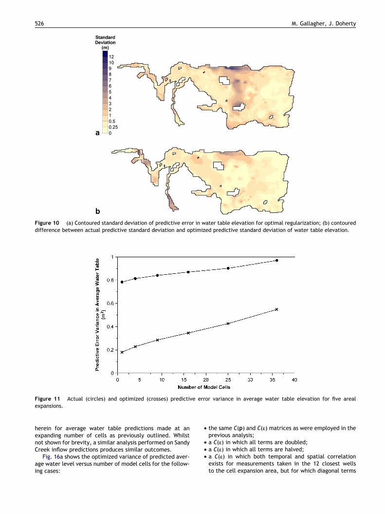
Minimized standard deviations of model-predicted headerrors over the entire model domain, calculated on the basisof optimized R and G matrices, are shown in Fig. 10a. Thedifference between actual predictive standard deviationsand optimized predictive standard deviations is shown inFig. 10b. While differences of between 0.5 m and 1.0 mare common, there are a few areas where the differenceis greater than this.

It is commonly stated that predictions made by a modelsuch as the Pioneer Valley model cannot be expected tohave precision on a cell-by-cell basis, but that average

Figure 8 (a) Model predicted water table elevation, and (b) contoured standard deviation of predictive error in water tableelevation.


heads over areas considerably larger than that of an individ-ual cell are likely to be predicted with greater precision. Totest this hypothesis, average heads, and the potential errorsassociated with these average heads, were calculated overa number of expanding square areas, starting with 1 celland increasing to 36. It was found that in some cases predic-tive error variance decreases whereas for others it in-creases, depending on conditions encountered by theexpanding averaging area. In general, if extra pumping wellsare encountered, and if these wells are strongly pumped,then error variance tends to rise rather than fall withincreasing area of averaging. However other factors can alsocontribute. The location of one of the cell expansions thatwas investigated is depicted in Fig. 1. Fig. 11 shows a plotof error variance versus number of cells for both actualand optimized R and Gmatrices. Expansion takes place fromthe top left to the bottom right of the square depicted inFig. 1 as cell numbers are increased from 1 to 36. Theexpansion takes place in a non-alluvial area from a cell thatis immediately adjacent to alluvium (where hydraulic prop-erty variance terms in the C(p) matrix are lower than thosefor non-alluvial areas) into an area of zero density of cali-bration observations.

Fig. 12a shows the contributions to optimized error var-iance from the first and second terms of Eq. (15) plottedagainst singular value number for each of the six differenthead predictions comprising averages over 1, 4, 9, 16, 25and 36 cells. As expected, the first (null space) term de-

creases with increasing singular value whereas the second(measurement noise) term increases. The total error vari-ance (Fig. 12b) shows a minimum, in this case at about290 singular values. As explained by Moore and Doherty(2005) the variance at zero singular value corresponds tothe square of pre-calibration predictive uncertainty. Theseplots show that the reduction in predictive error varianceattained through calibration is greater for smaller averagingareas than for larger average areas. This is a direct result ofproximity to alluvium and head measurement locations forcells employed in low-area head averaging in this particularexample.

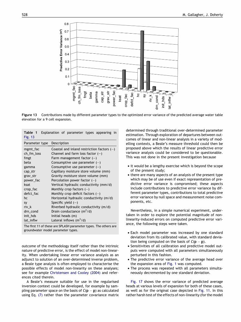
Fig. 13 shows the contribution to the optimized error var-iance of the predicted average head over nine cells by dif-ferent parameter types employed by the Pioneer Valleymodel. These contributions were calculated by fixing perti-nent parameter types (thereby assuming perfect knowledgeof them) and repeating the predictive error variance mini-mization process based on Eq. (15). The abbreviations em-ployed for the different parameter types cited in this plotare listed in Table 1. Five parameter types dominate pre-calibration predictive uncertainty (the back row variancesdepicted in this plot), two of which are SPLASH parametersand three of which are MODFLOW parameters. The calibra-tion process reduces to almost zero the contributions of allof these but hydraulic conductivity and specific yield. (Itmust be remembered that the examined prediction wasmade at the end of a dry period. If it had been made at

Figure 9 (a) Error variance of water table elevation predictions; (b) contribution from first term of Eq. (10) to predicted watertable error variance; (c) contribution from second term of Eq. (10) to predicted water table error variance.


the end of a wet period, the contribution by SPLASH param-eters may have been much higher.)

River inflowFig. 14 depicts predicted inflow on a cell-by-cell basis toSandy Creek plotted against cell number for the segmentof MODFLOW river cells upstream of the gauging stationshown in Fig. 1; cell numbering begins at the upstreamend of Sandy Creek. Also shown in Fig. 14 is riverbed con-ductance and cell inflow error standard deviation. It isapparent that calibrated riverbed conductance varies con-siderably along the length of the reach. Predictive errorstandard deviation is dependent on cell conductance, withsmaller errors being calculated in areas of smaller cell con-ductance. This may, in fact, be an outcome of the linearityassumption on which Eq. (10) is based. It is of interest tonote that the standard deviation of cell inflow predictive er-ror is many times higher than the actual inflow in such lowconductance regions, but is of the same order of magnitudeas inflow in high conductance regions.

In order to explore the affects of predictive averaging,average cell inflow to Sandy Creek was calculated for anincreasing number of cells, starting from 1 and increasing

in groups of 5 downstream to a total of 26 cells along thecreek segment indicated in Fig. 14. The error variance ofaverage Sandy Creek inflow is depicted in Fig. 15 for differ-ent numbers of cells over which averaging takes place. A de-crease in predictive error variance with increasing averagingis readily apparent from this figure.

Sensitivity analysisErrors in the assessment of predictive error variance canarise from a number of sources. Some of these are inherentin any methodology through which predictive error varianceis computed, most notably selection of suitable C(p) andC(e) matrices to employ in the analysis. (No analysis of errorvariance which recognises the inherent complexity of a nat-ural system can escape the use of some kind of stochasticdescriptor of this variability; nor can it forego characterisa-tion of the possible noise associated with measurementsfrom which system parameters are inferred.) A benefit ofthe methodology described herein is that computations ofpredictive error variance can be readily repeated with dif-ferent incidences of C(p) and C(e) so that the robustnessof error variance calculations in the face of limited knowl-edge of C(p) and C(e) can be tested. This is undertaken

Figure 10 (a) Contoured standard deviation of predictive error in water table elevation for optimal regularization; (b) contoureddifference between actual predictive standard deviation and optimized predictive standard deviation of water table elevation.

Figure 11 Actual (circles) and optimized (crosses) predictive error variance in average water table elevation for five arealexpansions.


herein for average water table predictions made at anexpanding number of cells as previously outlined. Whilstnot shown for brevity, a similar analysis performed on SandyCreek inflow predictions produces similar outcomes.

Fig. 16a shows the optimized variance of predicted aver-age water level versus number of model cells for the follow-ing cases:

• the same C(p) and C(e) matrices as were employed in theprevious analysis;

• a C(e) in which all terms are doubled;• a C(e) in which all terms are halved;• a C(e) in which both temporal and spatial correlationexists for measurements taken in the 12 closest wellsto the cell expansion area, but for which diagonal terms

Figure 12 (a) Contributions to the optimized error variance of averaged water table elevation from the first and second terms ofEq. (15). Downward sloping lines are the null space term, upward sloping lines are the measurement noise term; (b) total errorvariance of averaged water table elevations.


are the same as in the previous analysis. (For simplicity,correlation between measurements decays with distancefrom the diagonal of the C(e) matrix with a decay rate of0.95 per element; this simplistic correlation scheme isemployed solely to demonstrate the effect of a high levelof correlation between measurement errors on computedpredicted error standard deviations, and is not meant tobe a valid representation of true measurement noisecorrelation.)

Fig. 16b shows the optimized variance of predicted aver-age water level versus number of model cells for the follow-ing cases:

• the same C(p) and C(e) matrices as were employed in theprevious analysis;

• a C(p) in which all terms are doubled;• a C(p) in which all terms are halved;

• a C(p) in which hydraulic conductivity and specific yieldhave the same diagonal elements as in the previous anal-ysis, but for which spatial correlation shows an exponen-tial decay with distance, the decay constant being1000 m.

It is apparent from Fig. 16, that the error variance of pre-dicted head is somewhat sensitive to assumptions pertainingto C(p) and C(e), but not excessively so. The trend ofincreasing error variance with increased head averagingarea is maintained. Further analysis (not shown herein)demonstrates that computations of parameter contributionsto predictive error variance, and the extent to which theseare reduced through the calibration process, are reasonablyinsensitive to the shape and magnitude of C(p) and C(e)when varied by the same amount.

Another source of error in the computations presentedherein, and one of potentially greater concern as it is an

Figure 13 Contributions made by different parameter types to the optimized error variance of the predicted average water tableelevation for a 9 cell expansion.

Table 1 Explanation of parameter types appearing inFig. 13

Parameter type Description

mgmt_fac Coastal and inland restriction factors (–)ch_fm_loss Channel and farm loss factor (–)fmgt Farm management factor (–)beta Consumptive use parameter (–)gamma Consumptive use parameter (–)cap_str Capillary moisture store volume (mm)grav_str Gravity moisture store volume (mm)power_fac Percolation power factor (–)ksat Vertical hydraulic conductivity (mm/d)crop_fac Monthly crop factors (–)defct_fac Monthly crop deficit factors (–)hc Horizontal hydraulic conductivity (m/d)sy Specific yield (–)riv_k Riverbed hydraulic conductivity (m/d)drn_cond Drain conductance (m2/d)init_hds Initial heads (m)lat_inflw Lateral inflows (m3/d)

The first 11 of these are SPLASH parameter types. The others aregroundwater model parameter types.


outcome of the methodology itself rather than the intrinsicnature of predictive error, is the effect of model non-linear-ity. When undertaking linear error variance analysis as anadjunct to solution of an over-determined inverse problem,a Beale type analysis is often employed to characterise thepossible effects of model non-linearity on these analyses;see for example Christensen and Cooley (2004) and refer-ences cited therein.

A Beale’s measure suitable for use in the regularisedinversion context could be developed, for example by sam-pling parameter space on the basis of C(p � p) as calculatedusing Eq. (7) rather than the parameter covariance matrix

determined through traditional over-determined parameterestimation. Through exploration of departures between out-comes of linear and non-linear analysis in a variety of mod-elling contexts, a Beale’s measure threshold could then beproposed above which the results of linear predictive errorvariance analysis could be considered to be questionable.This was not done in the present investigation because

• it would be a lengthy exercise which is beyond the scopeof the present study;

• there are many aspects of an analysis of the present typewhich may be of use even if exact representation of pre-dictive error variance is compromised; these aspectsinclude contributions to predictive error variance by dif-ferent parameter types, contributions to total predictiveerror variance by null space and measurement noise com-ponents, etc.

Nevertheless, in a simple numerical experiment, under-taken in order to explore the potential magnitude of non-linearity-induced errors on computed predictive error vari-ance, the following steps were taken.

• Each model parameter was increased by one standarddeviation from its calibrated value, with standard devia-tion being computed on the basis of C(p � p).

• Sensitivities of all calibration and predictive model out-puts were computed with all parameters simultaneouslyperturbed in this fashion.

• The predictive error variance of the average head overthe expansion area of Fig. 1 was computed.

• The process was repeated with all parameters simulta-neously decremented by one standard deviation.

Fig. 17 shows the error variance of predicted averageheads at various levels of expansion for both of these cases,as well as for the original case depicted in Fig. 11. In thisrather harsh test of the effects of non-linearity (for themodel

Figure 15 Actual (circles) and optimized (crosses) predictive error variance of average Sandy Creek inflow over an increasingnumber of cells.

Figure 14 Predicted river cell inflow (triangles), standard deviation of river cell inflow error (crosses) and riverbed conductance(circles) for Sandy Creek.


can no longer be considered to be even approximately cali-brated with all parameters simultaneously varied by theamounts indicated), robustness of predicted head error vari-ance is reasonably good. Furthermore, the shape of thecurves is maintained. Further computations (not shown here-in) demonstrate that other qualitative aspects of the analysis(such as relativity of parameter contributions to pre- andpost-calibration predictive error variance, the reduction inthese contributions incurred by the calibration process, thenumber of singular values at which optimum predictive errorvariance is achieved, etc) are alsomaintained. Notwithstand-ing these results, the effects of model linearity on error var-iance computation (both in its quantitative and qualitativeaspects) is a subject that is worthy of further investigation.

Discussion

Integrity in model usage requires that some estimate of po-tential predictive error be supplied with model predictions

themselves. The methodology discussed herein allows suchestimates to be made with a high level of numerical effi-ciency. This is beneficial both in itself, and as a means ofinquiring into other aspects of the model construction andcalibration process. The authors of this paper feel thatthe ability to undertake such calculations relatively inex-pensively as a routine adjunct to model construction andcalibration could have profound implications for the wayin which models are employed in environmental manage-ment. Some of these implications are now briefly discussed.

The current trend in environmental modelling is formodels to become increasingly complex. Thus many modelsattempt to simulate many different environmental pro-cesses, and the interactions between these processes, at ahigh level of spatial and temporal detail. During the modelcalibration process a simplified parameterization schemeis often then ‘‘draped’’ over the complexities of the pro-cesses simulated by the model, this being done in order toreduce the number of model parameters to that which can

Figure 16 Optimized predictive error variance in average water table elevation for five areal expansions using the original C(e)and C(p) matrices (crosses) compared with (a) doubled C(e) terms (pluses), halved C(e) terms (circles) and a C(e) for which temporaland spatial correlation exists (squares); (b) doubled C(p) terms (pluses), halved C(p) terms (circles) and a C(p) for which spatialcorrelation exists in hydraulic conductivity and specific yield (squares).


be estimated on the basis of an often sparse calibrationdataset. The present study, and previous studies cited here-in, demonstrate that the ‘‘cost of uniqueness’’ incurred bydoing this is potentially a high level of model predictive er-ror. In fact it is not impossible that a seemingly complexmodel, on which is superimposed a simplistic parameteriza-tion scheme that ignores the complexity and variability ofthe real world, may in fact be no better a predictor of sys-tem behaviour than a simpler model, constructed at a frac-tion of the expense.

In spite of this, too often the decision is made to build acomplex model rather than a simple model, this decisioncommonly being based more on wishful thinking than on aproper understanding of the returns that will be gained fromconstruction of the complex model. In fact a complex modeldoes not guarantee integrity of predictions at all. What it can

guarantee, however, is integrity of predictive error analysis(for the null space term of Eq. (10) can then be properly de-fined). If such an analysis is not carried out, then the case forbuilding a complex model may indeed be questionable inmany modelling contexts. However if it is carried out in atleast one modelling exercise which is considered typical ofothers undertaken by a particular institution or agency, thenthat analysis may allow a suitable ‘‘engineering safety mar-gin’’ to be determined for future modelling exercises basedon simpler, less expensive models. Alternatively, becausesuch an analysis does not require the explicit use of measure-ments of system state, but only of the uncertainties associ-ated with such measurements, and because use of Eq. (15)does not require that the model be calibrated, it can beconducted before an expensive calibration exercise is com-menced, in order to judge the worth of that exercise.

Figure 17 Optimized predictive error variance in average water table elevation for five areal expansions using base parametervalues (crosses), a one standard deviation increase in base parameter values (circles) and a one-standard deviation decrease in baseparameter values (pluses).


Where a complex and expensive model is built as part ofan environmental management process involving differentstakeholder groups, it is essential that the model gainacceptance by these different groups if it is to fulfil the pur-poses for which it was constructed. The process of gainingacceptance often commences with the model constructionprocess itself, as discussions are held between, for exam-ple, modellers and regulators on the subject of what shouldbe included in the model, and what can be omitted from themodel, or represented only simply, without compromisingits predictive integrity. Using the methodologies presentedherein, such discussions can now take place on a much bet-ter scientific basis than in the past. For example, if it can beestablished through a relatively inexpensive pre-calibrationanalysis, that the contribution to the error variance of a keyprediction made by a particular boundary condition is rela-tively small, then this may put an end to arguments abouthow that boundary need be represented in the final model.It may allow agreement to be reached that a simplistic rep-resentation of that boundary is justified, based on assump-tions whose possible invalidity has few repercussions forpredictive integrity. This could result in reduced modelcost, both financial and emotional.

Use of the methodology discussed herein for optimiza-tion of data acquisition has already been mentioned. It isan easy matter to include in Eq. (15) terms pertaining tomeasurements of system state, or of system properties,that have not actually been made. As has been stated, theactual values of these system states or properties are notactually required in this analysis, only the uncertaintiesassociated with their measurement. In this manner, the effi-cacy of different measurement strategies can be comparedin terms of their ability to reduce the potential errors of keymodel predictions. Spending on data acquisition can therebybe placed on a more firm scientific footing than it otherwisewould be.

Perhaps the largest contribution that the methodologypresented herein can make to model-based environmental

management is through its ability to promote informed dis-cussion between different stakeholder groups. No longercan one group assert to another that ‘‘our model says thisand therefore it must be true’’. Groups that are subjectto environmental management by governing authoritieshave the right to know the potential error associated withassertions based on model outputs. With the availability ofa rapid means for quantification of possible model error,there is no longer any excuse for failing to provide such anassessment. If, after predictive error variance analysis hastaken place, predictive integrity can be shown to be high,then a model’s claim to special status in environmentalmanagement is sound; if it is not, then it will have becomeclear to all involved in the decision-making process that themaking of a definitive prediction of at least one aspect ofenvironmental behaviour may not be possible. If this is thecase, then decisions will have to be made by other means;if informed intuition rather than model outputs must formthe basis for important management decisions, this too willgain greater acceptance if model-based analysis indicatesthat there is no other alternative.

Conclusions

A methodology for calculation of the magnitude of potentialerror of any prediction made by a calibrated model has beenpresented. The method is perfectly general and requires noalterations to the model; it only requires that (a) model out-puts are not affected by any numerical misbehaviour on thepart of the model that compromises calculation of deriva-tives of these outputs with respect to adjustable parameters(normally using finite parameter differences), and (b) thatoutcomes of the analyses of most interest are not contami-nated unduly by model non-linearity. Because qualitativeaspects of the analysis will often be just as important asquantitative predictive error computations, the latter isnot expected to be a problem inmost groundwater modelling


contexts (and does not indeed appear to be a problem in thepresent context), though further analysis of this matter isrequired. The methodology can be applied to a model thathas already been calibrated and is actually being employedto make predictions. Or it can be applied to a model thathas not yet been calibrated, or has been only ‘‘approximatelycalibrated’’ using a simplistic parameterization scheme. Thisis possible because calculation of predictive error varianceusing this methodology does not require knowledge of actualfield measurements, only of the uncertainties associatedwith those measurements.

The methodology takes account of the two major con-tributors to model predictive error, namely the effects ofmeasurement error on parameter estimation error, andthe fact that there are strict limits on hydraulic property de-tail that can be inferred through the calibration process. Itis the authors’ experience, and it is indeed the case in theexample presented in this paper, that the latter contribu-tion can be substantial. In general, the more that a predic-tion depends on ‘‘system fine detail’’, the more that errorsin its prediction are likely to be dominated by this term.

The methodology is useful in its own right as a basis fortesting the veracity of predictions that may form the basisfor environmental management. As such it allows the useof modelling in environmental management to take placewith more integrity than has been done in the past. It canalso be used to judge the worth of undertaking an expensivemodelling exercise, in terms of the predictive accuracy thatis achievable on the basis of currently available data, beforethat exercise is actually undertaken. Alternatively, it can beused to optimize the acquisition of data in support of a mod-elling exercise, ensuring that newly acquired data is maxi-mally effective in raising the integrity of key modelpredictions.

Software

Software through which predictive error variance analysis ofthe type described herein can be implemented is suppliedwith the PEST suite. It can be downloaded free of chargefrom the following site: http://www.sspa.com/pest.

Acknowledgements

The authors would like to express their gratitude to NRWWater Assessment staff for numerous discussions and criti-cal revision undertaken during the course of the docu-mented study. Funding and logistical support provided byNRW is also gratefully acknowledged.

References

Arunakumaren, N.J., 1997. A lumped parameter model for simu-lating the temporal behaviour of moisture in the plant root zoneand in the unsaturated zone below the root zone. LWRRDC R&DProject QP127. Department of Natural Resources and Mines,Queensland Government, Brisbane.

Carrera, J., Glorioso, L., 1991. On geostatistical formulations of thegroundwater flow inverse problem. Adv. Water Resour. 14 (5),273–283.

Carrera, J., Alcolea, A., Medina, A., Hidalgo, A., Slooten, L., 2005.Inverse problem in hydrogeology. Hydrogeol. J. 13, 206–222.

Certes, C., de Marsily, G., 1991. Application of the pilot pointsmethod to the identification of aquifer transmissivities. Adv.Water Resour. 14 (5), 284–300.

Christensen, S., Cooley, R.L., 1999. Evaluation of predictionintervals for expressing uncertainties in groundwater flowpredictions. Water Resour. Res. 35 (9), 2627–2639.

Christensen, S., Cooley, R.L., 2004, User guide to the UNC processand three utility programs for computation of nonlinear confi-dence and prediction intervals using MODFLOW-2000: US Geo-logical Survey Techniques and Methods Report 6-A10, USGeological Survey, Reston, VA, 195 pp.

Cooley, R.L., 2004. A theory for modeling ground-water flow inheterogeneous media. Professional Paper 1679, US GeologicalSurvey, Reston, VA, 229pp.

De Groot-Hedlin, C., Constable, S., 1990. Occam inversion togenerate smooth, 2-dimensional models from magnetelluricdata. Geophysics 55 (12), 1613–1624.

Doherty, J., 2003. Groundwater model calibration using pilot pointsand regularization. Ground Water 41 (2), 170–177.

Doherty, J., 2005. PEST: Model independent parameter estimation.Watermark Numerical Computing, Corinda, Australia. <http://www.sspa.com/pest>.

Doherty, J., Gallagher, M., 2005. Analysis of predictive error of thePioneer Valley groundwater model. Watermark Numerical Com-puting, Brisbane, Australia. A copy of this report in PDF formatcan be supplied by either of the authors on request.

Eden, R.N., Hazel, C.P., 1973. Computer and graphical analysis ofvariable discharge pumping tests of wells. The Institution ofEngineers Australia. Civil Engineering Transactions, pp. 5–10.

El Harrouni, K., Ouazar, D., Wrobel, L.C., Cheng, A.H.-D., 1997.Uncertainty analysis in groundwater flow with DRBEM. Eng. Anal.Bound. Elem. 19, 217–221.

Gomez-Hernandez, J.J., Franssen, H.J.W.M.H., Sahuquillo, A.,2003. Stochastic conditional inverse modeling of subsurfacemass transport: a brief review of the self-calibrating method.Stoch. Environ. Res. Risk A 17, 319–328.

Gutjahr, A., Bras, R.L., 1993. Spatial variability in subsurface flowand transport – a review. Reliab. Eng. Syst. Safe. 42 (2–3), 293–316.

Harbaugh, A.W., Banta, E.R., Hill, M.C., McDonald, M.G., 2000. TheUS Geological Survey Modular Ground-Water Model – User Guideto Modularization Concepts and the Ground-Water Flow process.US Geological Survey Open File Report 00-92. Reston, VA.

Hill, M.C., 1989. Analysis of accuracy of approximate, simultaneous,nonlinear confidence intervals onhydraulic heads in analytical andnumerical cases. Water Resour. Res. 25 (2), 177–190.

Kitanidis, P.K., 1995. Recent advances in geostatistical inference onhydrogeological variables. Rev. Geophys. 33, 1103–1109.

Kuhanesan, S., Durick, A., Werner, A., Weeks, S., Murphy, S., 2005.Groundwater amendment to the Pioneer Valley Water ResourcesPlan. Report 3: Groundwater flow modelling of the PioneerValley. Water Assessment, Resource Condition and Trend.Natural Resource Sciences, Queensland Department of NaturalResources, Mines and Water.

Moore, C., 2006. The use of regularised inversion in groundwatermodel calibration and prediction uncertainty analysis. Ph.D.Thesis, University of Queensland, Australia.

Moore, C., Doherty, J., 2005. Role of the calibration process inreducing model predictive error. Water Resour. Res. 41,W05020. doi:10.1029/2004WR00350.

Moore, C., Doherty, J., 2006. The cost of uniqueness in groundwatermodel calibration. Adv. Water Resour. 29 (4), 605–623.

Murphy, S., Kuhanesan, S., Foster, L., Durick, A., 2005. Groundwa-ter amendment to the Pioneer Valley Water Resources Plan.Report 1: Conceptualisation of groundwater resources for thePioneer Valley flow model. Water Assessment, Resource Condi-

http://www.sspa.com/pest



http://dx.doi.org/10.1029/2004WR00350


tion and Trend, Natural Resource Sciences, Queensland Depart-ment of Natural Resources, Mines and Water.

Poeter, E.P., Hill, M.C., 1998. Documentation of UCODE, acomputer code for universal inverse modelling. US GeologicalSurvey Water. Resources Investigation Report 98-4080, p. 122.

Tonkin, M., Doherty, J., 2005. A hybrid regularised inversionmethodology for highly parameterised models. Water Resour.Res. 41, W10412. doi:10.1029/2005WR00399.

Vecchia, A.V., Cooley, R.L., 1987. Simultaneous confidence andprediction intervals for nonlinear regression models with appli-cation to a groundwater flow model. Water Resour. Res. 23 (7),1237–1250.

Yeh, T.C.J., 1992. Stochastic modeling of groundwater-flowand solute transport in aquifers. Hydrol. Process. 6 (4), 369–395.

Zimmerman, D.A., de Marsily, G., Gotway, C.A., Marietta, M.G.,Axness, C.L., Beauheim, R.L., Bras, R.L., Carrera, J., Dagan, G.,Davies, P.B., Gallegos, D.P., Galli, A., Gomez-Hernandez, J.,Gorelick, S.M., Grindrod, P., Gutjahr, A.L., Kitanidis, P.K.,LaVenue, A.M., McLaughlin, D., Neuman, S.P., RamaRao, B.S.,Ravenne, C., Rubin, Y., 1998. A comparison of seven geostatis-tically based inverse approaches to estimate transmissivities formodeling advective transport by groundwater flow. WaterResour. Res. 34 (6), 1373–1413.

http://dx.doi.org/10.1029/2005WR00399

Date post:	26-Oct-2016
Category:	Documents
Upload:	mark-gallagher
View:	214 times
Download:	1 times

Predictive error analysis for a water resource management model

Documents