Predictive maintenance by the identification of suspensionparameters from inline acceleration measurements

S. Kraft∗,∗∗, C. Funfschilling∗, G. Puel∗∗, D. Aubry∗∗∗ SNCF, Direction de l’Innovation et de la Recherche, 45 rue de Londres, 75379 Paris∗∗ Laboratoire MSSMat, Ecole Centrale Paris/CNRS UMR 8579, Grande Voie de Vignes, 92295Châtenay Malabrye-mail: sonke.kraft@sncf.fr

AbstractThis work proposes the application of model-based condition monitoring on railway vehicles. Byidentifying the parameter values of a multi-body model of the vehicle from measurement data,changes in suspension parameters due to defects or wear could be detected. As a test case, theparameter identification is applied to a model of a railway bogie. This allows to have a modelwith known dynamic equations which represent the geometric nonlinearity of the wheel rail contactand suspension elements. For the identification of the suspension parameters different methods aretested. Of particular interest is the adjoint state method for the calculation of the cost functiongradient used in gradient-based optimisation methods.

1 Introduction

Today the maintenance of trains is calendar-based. Elements exposed to important loads are ex-changed after a defined period of time or kilometers. The choice of the maintenance intervals isbased on theoretical considerations but mainly on experience. In order to guarantee the securityand comfort of the vehicle, the maintenance intervals are chosen with great care. Sometimes thismay lead to maintenance intervals being too short.In order to reduce the immobilisation time of the vehicle and improve the reliability while assuringthe safety demands, a condition-based maintenance is envisaged. The basic idea is to change anelement not after a predefined interval but depending on the actual condition of the element. Thisrequires the detection of changes in the dynamic properties of the element during operation.The technique to analyse the actual dynamic behaviour of a vehicle during operation is known ascondition monitoring. It is based on measurements during operation and an analysis in order toidentify changes in the vehicle dynamics indicating defects.Different approaches for condition monitoring exist. Up to now it is based mainly on the signalprocessing of measured acceleration data. Limit values are checked and a frequency analysis isperformed in order to detect defects in elements. A widely used application is the measurementof axle box accelerations for the detection of wheel defects like wheel flats or unroundness [11].Another objective is the identification of running instability from bogie condition monitoring [13].A sophisticated approach is model-based condition monitoring. It is based on the idea to representthe real system by a model and to identify the model parameters from measurements. The approachis discussed in [6] and [13].The aim of the French railway company SNCF is to extend the application range of the conditionmonitoring. Beside the bearings and wheels, the elements of the primary and secondary suspension

3503

are exposed to high dynamic forces. There is an interest in estimating the parameters and changesin some suspension elements from condition monitoring. Notably rubber spring elements in theprimary suspension and hydraulic dampers like the anti-yaw damper are of interest.This work proposes to study the potential of model based-condition monitoring for a multi-bodymodel of a railway bogie. It has the aim to identify changes in the parameter values of the suspension.In section 2 the technical context is outlined. Then in section 3 the multi-body model of the bogie ispresented. The parameter identification procedure is described in sections 4 and 5. Then in section6 the results of the parameter identification are presented.

2 Condition monitoring

The aim of the condition monitoring approach discussed in this work is the identification of pa-rameter changes for the suspension elements which have an important influence on the dynamicbehavior of the vehicle. Concerned suspension elements are mainly rubber spring elements andhydraulic dampers. Coil springs do normally not underlie wear or damage leading to parameterchanges.Rubber spring characteristics can change due to material deterioration but there are no verifiedcalculation methods for the evaluation of their life-time. Up to now these elements are replacedpreventively after a defined amount of kilometers.Hydraulic dampers are widely used in the primary and secondary suspension. By damping vibrationsthey assure the safety and comfort of the vehicle. Despite the high reliability of hydraulic dampers,defects can appear which change the dynamic properties of the damper and the vehicle behavior.Possible failures are defect valves, defect seals or loose mountings. The maintenance procedure usedtoday is to dismount regularly the dampers and to test them on a test rig.As mentioned in the introduction, condition monitoring systems based on signal processing arealready used for the identification of wheel-flats or running instabilities. However, a parameterestimation exclusively based on signal processing is difficult to perform. It would require the mea-surement of accelerations and forces in every suspension element. Besides, the dynamic couplingbetween several elements is difficult to consider.Model-based techniques seem therefore more suitable. Two types of models can be used: data-basedmodels and theoretical models. Data-based modeling tries to express the measured accelerationdata by an analytical regression model. The parameters of regression models do not have a physicalmeaning. It is not possible to relate them to the different suspension elements of the bogie.A physical model instead is based on the mechanical structure and physical principles of the sys-tem. It allows to relate the parameters of the model to the elements of the system and to locatethe reason for changes in the dynamic behavior. For questions concerning the low frequency dy-namics of railway vehicles, this approach consists in representing the train by a multi-body model.Wheelsets, bogies and car bodies are represented by rigid bodies and the suspension elements aremodeled by rheological models. By minimizing the difference between the model results and themeasured responses, the parameter values are estimated. At SNCF dynamic measurements havebeen performed in a high speed train TGV Duplex on the TGV east line. Accelerations are availablein the axle boxes, bogie and car bodies. The track irregularities are measured with high precisionfrom the IRIS320 measurement train. The model used is a multi-body model of the TGV Dupleximplemented in the commercial software Vampire.However, the use of physical models for parameter estimation and error detection also brings alongsome difficulties. A crucial point is that only parameters and defects which can be represented bythe model are found . The estimation of parameters and the locations of defects demand a detailed

3504 PROCEEDINGS OF ISMA2010 INCLUDING USD2010

model with a high precision. This requires in turn a precise knowledge of the system and all itscomponents. For a complex system like a train the design of such a precise model is a difficult task.Another difficulty is the consideration of errors and uncertainties in the model. If the knowledgeon uncertainties, noise and unknown excitation is incomplete or not available, the use of a physicalmodel is complicated. And finally measurements needed for the estimation of model parameterscan be incomplete.To start the model-based parameter identification and defect detection directly for the complexmodel of the complete TGV train seems therefore unsuitable. Instead we propose in this workto study the potential of parameter identification and defect detection on a simpler model whichrepresents only one bogie. Since no acceleration measurements are available for a single bogie, acalculation is used as a reference instead of the measurements. This allows to validate the resultsfor the parameter estimation and defect detection since the true parameter values and introducedeffects are known a priori. In the next section the model and its properties are described.

3 Model of a bogie

In this work the multi-body model of a bogie is used as a test case. The model is implementedin Matlab. Two aims are pursued. The first is to have a simple multi-body model with a knownanalytical description allowing the application and comparison of different identification methods.The second aim is to have a model which takes into account the important dynamic characteristicsof railway vehicles, notably the wheel-rail contact and its geometric nonlinearity as well as thenonlinear suspension elements.The bogie model is composed by three bodies: the bogie frame and two wheelsets. It is running onthe track with a constant speed. The model is excited by the track irregularities spatially measuredalong the track. The track irregularities considered are the vertical and horizontal displacement ofthe right and the left rail. Otherwise the track is supposed to be rigid. In figure 1 the structure ofthe model is shown.

3.1 Kinematics

Under the assumption that the centres of gravity of the wheelsets move with a constant speed v,two degrees of freedom are identified for each wheelset: the lateral displacement uy and the rotationaround the z axis δz. This assumption is justified since mainly lateral effects determine the dynamicof the wheelset. Finally, 10 degrees of freedom are identified for the model: two for each wheelsetand six for the bogie frame. The vector of generalised coordinates composed of the degrees offreedom is:

x = (rbx, rby, rbz, δbx, δby, δbz , ue1y, ue2y, δe1z , δe2z)T (1)

with:rbx, rby, rbz: bogie position, δbx, δby, δbz: bogie rotation, ue1y, ue2y: lateral displacements of the

wheelsets, δe1z , δe2z: yaw rotations of the wheelsets.The kinematic equations describe the position of the wheelset and the contact points respectivelyas functions of the degrees of freedom. For real profile combinations these relations become verycomplicated and can not be expressed in analytical form. In order to obtain an analytic mathematicdescription, for this model a circular rail profile and a conical wheel profile are used.After the definition of the independent coordinates the next and difficult step is to relate thedependent coordinates to the degrees of freedom. Beside the position parameters for the centre ofgravity, two values are important for the dynamic calculations of the vehicle: the left and right

RAILWAY DYNAMICS AND GROUND VIBRATIONS 3505

Figure 1: Model of the bogie including two wheelsets

contact radii rl(r) and the angle δl(r) in the contact point. The calculation of these kinematicrelations is relatively complicated and not outlined here. It results in nonlinear equations whichcan be found in [5]. By applying a Taylor development these relations are linearized except forthe vertical displacement where quadratic terms persist. The position of the wheel-set relative tothe inertial system depends also on the track irregularities, expressed by the vertical displacementdz, a horizontal displacement dy and a cross level irregularity of the track γd relative to its idealposition. Taking into account the track irregularities in the kinematic relations obtained for thevertical displacement uz, the angle δx, the contact radii rl(r) and the contact angle δl(r) are givenby:

uz = dz −12r0(γd)2 + 1

2ζ(uy − dy + r0γd)2 − 12ξδ

2z (2)

δx = γd + σ 2e0

(uy − dy + r0γd) (3)

rl(r) = r0 ± λ(uy − dy + r0γd) (4)

tan δl(r) = tan δ0 ± ε2e0

(uy − dy + r0γd) (5)

λ, ε, σ, ζ and ξ: geometry parameters defined in [5]

3.2 Equations of motion

Outgoing from these kinematic relations the equations of motion are calculated using the Lagrangeapproach. It is based on the kinetic energy of the system and has the form:

d

dt(∂Ec∂qj

)− ∂Ec∂qj

= dj , j = 1, ...., 10 (6)

3506 PROCEEDINGS OF ISMA2010 INCLUDING USD2010

Ec is the kinetic energy of the system calculated with the translational vi and rotation velocities ωifor every body described by its mass mi and inertia Ji:

Ec = 12

3∑i=1

(vTi mivi + ωTi JiPωi) (7)

The generalized forces d of the Lagrangian equations are calculated with the forces fEi and momentsmEiP acting on every body and the Jacobian matrices of translation JT i and rotation Jri:

d =3∑i=1

(JTT ifEi + JTrimEiP ) (8)

The vector d of the generalized forces is composed of the spring and damping forces of the primarysuspension and the friction forces of the wheel-rail contact. The spring and damping forces arecalculated using the displacements and velocities at the coupling points of the suspension expressedin inertial coordinates.The friction forces are related to the slip in the contact surface between wheel and rail through thecoefficient of friction. The slip is defined as the relative velocity in the contact point normalized bya reference velocity. Three different slips are distinguished: the lateral slip νξ, the vertical slip νηand the rotational slip νζ . They are represented in figure 2.

(a) (b)

Figure 2: Relative velocities: top view (a) front view (b) with velocity terms (1) to (5)

vr(l)ξ = rr(l)Ω cos δz ± δze0/2 − v (9a)

vr(l)η = rr(l)Ω sin δz cos δr(l)︸ ︷︷ ︸(1)

− ddt

[(uy − dy + r0γd) cos δr(l)]︸ ︷︷ ︸(2)

− ddt

[δx(e02 sin δ0 + rr(l)cosδ0)]︸ ︷︷ ︸

(3)

(9b)

vr(l)ζ = ±Ω sin δr(l)︸ ︷︷ ︸

(4)

− ddt

[δzcosδr(l)]︸ ︷︷ ︸(5)

(9c)

For the calculation of the friction forces and moments, the linearized Kalker theory [3] is applied.It assumes that the slip rates are small so that a linear ratio between slip and friction force can beapplied. The values for the Kalker coefficients Cij depend on the form of the contact ellipse andcan be found for example in [5]. TξTη

Mζ

= Gab

C11 0 00 C22

√abC23

0 −√abC23 abC33

=

νξνηνζ

(10)

RAILWAY DYNAMICS AND GROUND VIBRATIONS 3507

with: G: shear modulus

The form of the contact surface is elliptic and described by the contact radii a and b. They areobtained from the Hertz theory of the normal contact problem [2]. The Hertz theory allows tocompute for a known normal force the contact radii, the elastic deformation and the stress in thecontact surface. Input parameters are the radii of curvature for the rail and the wheel and themodulus of elasticity. The normal force is composed by static forces due to the mass and a dynamicpart.Finally, the nonlinear equations of motion for the bogie model are obtained from the Lagrangianequations in the form:

M(x, t)x(t) + g(x, x, t) = d(x, x, t) (11)

M is the mass matrix and depends generally on the parameter vector x and time. g regroups allnonlinear termes depending on the parameter vector x and its first derivative x. d is the nonlinearvector of generalized forces. It is not possible to solve this equation system analytically. Numericalintegration algorithms have to be used instead.The forward model allows to analyse the dynamic behavior of the bogie model. Although it isrelatively simple, important properties of vehicle track systems are reproduced. If the lateral dis-placement and the rotation of the wheelsets are plotted, the typical hunting movement is found.Below the so-called critical speed the wheelset behaves stable and the oscillation decays. If thevehicle speed is increased and the critical speed is attained the behavior changes abruptly. An ini-tial displacement leads to an oscillatory movement with increasing amplitude. The system becomesunstable.

4 Parameter Identification

4.1 Cost function criteria

After a model has been chosen one can turn towards the second step, the parameter identification.The aim is to identify the parameters of the model so that the model results coincide best with themeasured results. Outgoing from an initial estimation of the model parameters the identificationalgorithms seek to minimize the differences between the model and the measurements, expressedby a cost function.Based on the properties of the model including parameters with a physical meaning and nonlin-earities, the structural model updating has been chosen as the identification method. It is a timedomain method comparing the dynamic response of the model with the measured response. Thisis done by defining a cost function which quantifies the distance between the time signals. Mostcommonly, quadratic cost functions based on least squares are used. For every time step the errore(t) between model and measurement is computed e(p, t) = xmeas(t)−xmodel(t, p) and the L2 normis integrated or summed over the time length T:

Jls(t, p) =∫ T

0eT (p)We(p)dt (12)

W is a weighting matrix defining the relative importances of the different acceleration channels onthe cost function.For the parameter identification it is important to consider if the problem is constrained or uncon-strained. In an unconstrained problem the parameters can take any value while for a constrainedproblem their values are restricted to a predefined range. It is obvious that the problem consideredhere is constrained. The parameters have a physical meaning describing properties of suspension

3508 PROCEEDINGS OF ISMA2010 INCLUDING USD2010

elements. Their values are limited to a certain range around the target value which corresponds tothe tolerance assured by the manufacturer.

4.2 Parameter sensitivity

Before choosing the parameters for the identification process an important question has to beconsidered: which parameters are identifiable from the available measurement data?Only parameters which have an influence on the defined cost function are identifiable. The questionwhich parameters have an impact on the cost function can be answered by performing a sensitivityanalysis. In a first step, the cost function is defined. For the bogie model the displacements inthe bogie frame are chosen. Then the identifiability of all system parameters relative to thesedisplacements is studied.It can be distinguished between local and global sensitivity analysis [10]. The factor screeningmethod is a local deterministic method where only one parameter is varied while the others are heldconstant. The variation is performed between a minimal and maximal value in defined steps. Thisapproach allows to calculate the influence of one parameter on the cost function. Its advantage isthe graphical representation of the solution surface of the cost function.However, the sensitivity obtained from the deterministic screening approach has several drawbacks.The influence of a parameter on the cost function does not only depend on the gradient but alsoon the variability of the parameter expressed by its variance. In order to consider the variability ofthe parameter values the sensitivity analysis has to be based on the variances.Besides, the screening method can not take into account interactions between several parameterson the cost function. This is especially important for models which are not linear in its parametersas it is the case for the bogie model. The superposition principle is not fulfilled and the effect ofchanging two parameter values is different from the sum of their individual effects. In the case oftwo parameters this interaction can be illustrated graphically by a three-dimensional plot showingthe cost function relative to two parameters as shown in figure 4. Evidently, the sensitivity obtainedfrom the screening method is only valid for one parameter set with fixed values.In order to overcome these limitations probabilistic global methods are used which can take intoaccount the parameter variances and the interactions in nonlinear models. They allow all inputparameters to vary simultaneously by treating the input parameters as random variables with anassumed probability density distribution. For this work the importance factors of each parameterare calculated using the Sobol-method. It is based on repeated Monte-Carlo calculation with oneparameter fixed. Importance factors are calculated from the reduction of the cost function variancedue to the fixed parameter.

5 Optimisation methods

When the cost function criterion is defined and the parameters are chosen as a result of the sensitivityanalysis, the optimization can be applied. It is the crucial step of the parameter identification andaims to minimize the cost function J in order to identify the parameter values of the model.Many different optimization methods exist ([1],[8],[9]). In order to choose methods which areadapted to the suspension parameter identification problem, the important properties of the problemhave to be considered.One question concerns the number of parameters. It depends on the complexity of the model. Forthe bogie model the number of parameters of the suspension depends on the description used forthe suspension elements. Since only one bogie is considered it stays relatively small. However,

RAILWAY DYNAMICS AND GROUND VIBRATIONS 3509

considering that the bogie model is studied as a test case for a much more complex model of thecomplete train with far more than 100 parameters, the effect of an important number of parametersis taken into account.Although only the parameters which have an effect on the considered cost function are includedin the identification procedure, this effect can be very unequal. The optimisation method has toaccount for this by normalizing the parameter values for example.Finally the shape of the hypersurface described by the cost function is important. If the costfunction is convex, local optimisation methods can be applied. They are based on the calculation ofthe gradient of the cost function. Since only one minimum exists on the solution surface, gradient-based methods are able to converge to this minimum from every starting point.For many complex systems this condition is not fulfilled. The cost function has several so-calledlocal minima. The aim of the optimisation algorithm is therefore to identify the minimum with thelowest cost function value. This minimum is called global minimum. Local optimisation methodsonly converge to the global minimum if the initial value is already in its attractor space. Instead,if the start value is close to a local minimum the local method converges to this local minimum.Since the solution of the cost function and therefore the positions of local and global minima areusually not known a priori, local methods are not able to identify the global minium. In this caseglobal methods have to be used.

5.1 Local methods

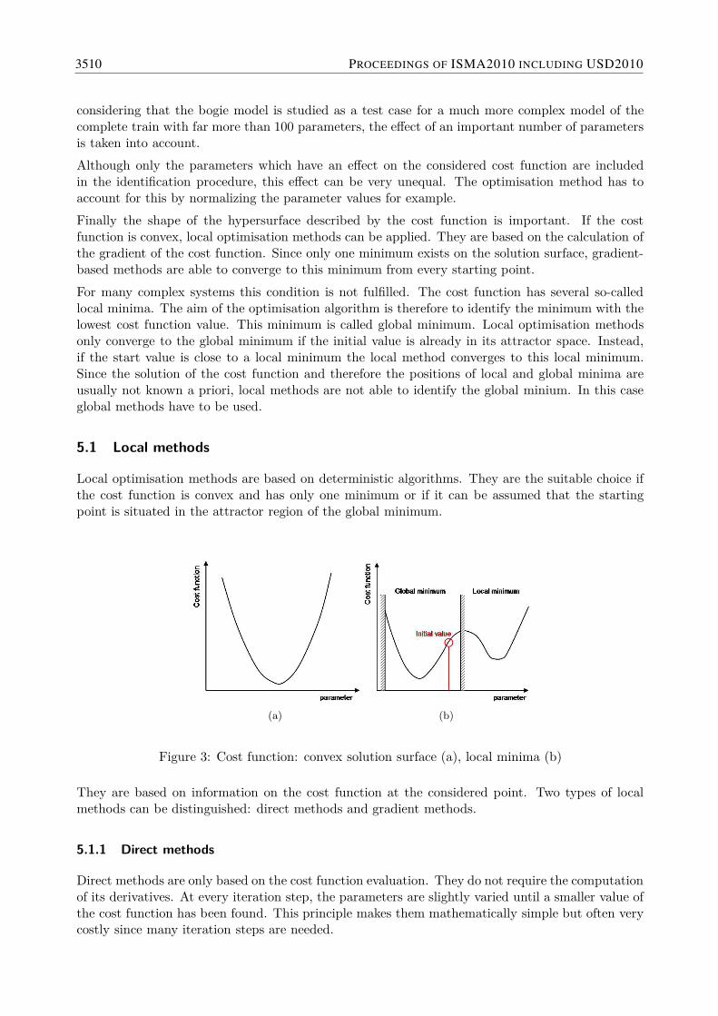
Local optimisation methods are based on deterministic algorithms. They are the suitable choice ifthe cost function is convex and has only one minimum or if it can be assumed that the startingpoint is situated in the attractor region of the global minimum.

(a) (b)

Figure 3: Cost function: convex solution surface (a), local minima (b)

They are based on information on the cost function at the considered point. Two types of localmethods can be distinguished: direct methods and gradient methods.

5.1.1 Direct methods

Direct methods are only based on the cost function evaluation. They do not require the computationof its derivatives. At every iteration step, the parameters are slightly varied until a smaller value ofthe cost function has been found. This principle makes them mathematically simple but often verycostly since many iteration steps are needed.

3510 PROCEEDINGS OF ISMA2010 INCLUDING USD2010

Important representatives of direct methods are the simplex and pattern search methods [12]. Thepattern search method is widely used due to its good convergence properties, low memory demandand simple algorithmic structure.

5.1.2 Gradient methods

A faster convergence is obtained if information about the derivatives of the cost function is used.This is the main feature of gradient methods. They use the gradient and optionally the Hessianmatrix of the cost function for the determination of the search direction.Two different groups of gradient methods can be distinguished. Line search methods ([8], [1])are based on a unidimensional minimization along the search direction. In a first step the searchdirection in which the cost function decreases is determined. Then a unidimensional minimization isperformed along this direction. The second group spans the trust region methods. They are basedon the definition of a trust region around the actual parameter value in which the cost function canbe approximated by a quadratic function. Then the minimum in this region is sought.

5.2 Methods for the calculation of the gradient

All gradient methods require the calculation of the gradient. Especially for complex systems witha large number of parameters, the gradient calculation represents the most expensive step in theoptimisation algorithm. The choice of an adapted method for the calculation of the gradient istherefore crucial and will be outlined in the following section.Evidently, a simple but rarely the best way of obtaining approximated numerical values of the costfunction gradient is the finite differences method.

D+hJ(p) = J(p+ h)− J(p)h

(13)

For a large number of parameters this method is very costly. Besides, the choice of the step-length his difficult. If h is too large, then truncation errors become significant. Even if h is optimally chosen,the derivative of the cost function J will be accurate to only about 1/2 or 2/3 of the significantdigits of J .Therefore alternative calculation methods should always be taken into account. If the equations ofmotion describing the system are available, analytical approaches can be used. In this work theadjoint state method which is in particular adapted to systems with a large number of parametersand algorithmic differentiation methods are used.

5.3 Adjoint state methods

The adjoint method is an analytical approach for the calculation of the gradient. The main advan-tage of the adjoint state method is that its complexity does not depend on the number of parameters.This makes it suitable for problems with a large number of parameters [7].The aim of the adjoint method is to calculate the gradient of the cost function J(x(p), p) in orderto minimize the cost function:

∇piJ(x(p), p) for i = 1...n (14)

n: number of parameters

RAILWAY DYNAMICS AND GROUND VIBRATIONS 3511

The cost function depends on the parameters pi and on the response x(p) of the system. The totalderivative of the cost function with respect to the parameters pi is therefore:

dJ

dpi= ∇piJ(x(p), p) +∇xJ(x(p), p) (15)

The derivatives of the result of the forward model x with respect to the parameters are not known.Due to the complexity of the nonlinear model an analytical calculation is not possible.In order to overcome this problem the following approach is used: instead of minimizing the costfunction J the stationarity of the Lagrangian equation L given by the sum of the cost function andthe state equation is seeked. The stationarity of the Lagrangian equation implies the minimizationof the cost function. It is supposed that the variables p, x and z in the Lagrange equation areindependent giving the derivative:

dL(p, x, z) = ∇pL(p, x, z)dp+∇xL(p, x, z)dx +∇zL(p, x, z)dz (16)

In the following this approach is illustrated for the bogie model. In section 3 the nonlinear equationof motion was found to be:

M(x, p)x(t) + F (x, x, p, t) = 0 (17)

From the Lagrange equation L the gradient and the adjoint state equation are calculated. TheLagrange equation has the form:

L = J(p) +∫ T

0(z,M(x, p)x(t) + F (x, x, p, t)) = 0 (18)

For the cost function the difference between measured and simulated displacements is used. Thegradient equation is therefore:

∇pL =∫ T

0(Dp(Mx)T z +DpF T z)dt = 0 (19)

The derivative of the Lagrange equation with respect to x gives the adjoint state equation:∫ T0

(z,DxMxδx)dt+∫ T

0(z,Mδx)dt+

∫ T0

(z,DxFδx)dt+∫ T

0(z,DxFδx) =

∫ T0

(x−xexp)δxdt (20)

In the next step the derivatives of x should be separated and the terms integrated by parts in orderto eliminate all derivatives of δx from the adjoint state equation.∫ T

0(DxMxδx, z)dt =

∫ T0

((DxMx)T z, δx)dt (21a)∫ T0

(Mδx, z)dt =∫ T

0(MT z, δx)dt = [(MT z), δx]T0 − [ ˙(MT z), δx]T0 +

∫ T0

( ¨(MT z), δx)dt (21b)∫ T0

(DxFδx, z)dt =∫ T

0(DxF T z, δx)dt (21c)∫ T

0(DxFδx, z)dt =

∫ T0

(DxF T z, δx)dt = [DxF T z, δx]T0 −∫ T

0((DxF T z)•, δx)dt (21d)

The adjoint equation is therefore given by:

¨(MT z) + (DxMx)T z + (DxF T )z − (DxF T z)• = x− x0 (22)

In the adjoint state equation several derivatives of the matrix M appear:

MT z +MT z + 2MT z + (DxMx)T z + (DxF T )z − (DxF T )•z −DxF T z = x− x0 (23)

3512 PROCEEDINGS OF ISMA2010 INCLUDING USD2010

Under the condition that the remaining terms cancel each other, the final conditions are:

z(T ) = 0 (24a)z(T ) = 0 (24b)

The term DxM describes the derivative of the matrix M with respect to a vector x giving a tensorof order 3. If the derivative of M is contracted with the vector x a second order tensor is obtained:

(∂mi,j∂xsei ⊗ ej ⊗ es)x = ∂mi,j

∂xs(es, x)ei ⊗ ej = ∂mi,j

∂xs(xs)ei ⊗ ej (25)

Accordingly, an index appearing twice in a multiplicative term represents a summation. The equa-tion above can therefore be written as: ∑

s

xs∂mi,j∂xsei ⊗ ej (26)

For the validation of the adjoint state method the scalar product test proposed in [4] is used. Itis based on the definition of the adjoint state. At first the differentiated equation of the system issolved for an arbitrary excitation.

(DxMx)δx+Mδx+DxFδx +DxFδx = b(t) (27)

The result for δx is injected on the right side in the adjoint state equation (23) and the followingscalar products (b, z) and (δx, δx) are calculated. If the two scalar products give the same resultfor different choices of b the result of the adjoint equation is validated.

5.4 Global methods

For complex systems the cost function is often a nonlinear function with several minima. Thenlocal optimisation methods can possibly fail. In this case global methods which are able to leavethe attractor region of a local minimum in order to converge to the global minimum of the solutionspace have to be used. In order to do so, global methods can not be exclusively deterministic. Onlyif an increase of the cost function value is accepted with a certain probability the method is able toleave a local minimum.All global methods include therefore a probabilistic operator. In the simulated annealing method[12] used in this work the probability for the acceptance of increased cost function values dependson a parameter called temperature. The method simulates the cooling process of a material.

6 Results

In order to use the estimations of the vehicle suspension parameters for condition monitoring pur-poses, a high precision is required. For the real system this evaluation is difficult to perform sincethe model results are compared with measurements for which the real parameter values are notknown.For the bogie model developed here no measurement data from a real system are available. Thislimits the informative value of the model but allows to study the different parameter identificationmethods and their applicability to condition monitoring methods.At first, the identifiability of the suspension parameters is analysed by a sensitivity analysis. Thenthe parameter identification methods outlined above are applied to the parameters which have aninfluence on the dynamic response of the bogie model.

RAILWAY DYNAMICS AND GROUND VIBRATIONS 3513

6.1 Sensitivity Analysis

The identifiability of the parameters is obtained by a sensitivity analysis. One parameter is modifiedwhile the others are fixed. This approach can be extended to the 3-dimensional case shown in figure4 where 2 parameters vary simultaneously pointing out interactions between the two parameters.

0

5

10x 107 0

5

10

x 106

0

0.5

1

1.5

2

2.5

x 10−3

cycx

cost

Figure 4: Screening for parameters cx and cy

Interactions between the parameters are taken into account by global methods. It is found that forthe model with a linear spring and damper only the spring stiffness have an influence on the modelresult. Beside, due to the nonlinearity of the model the interactions between the parameters areimportant.

6.2 Minimization of the cost function

The optimisation methods presented in section 5 have been compared. For the important group ofgradient-based methods the calculation of the cost function gradient with respect to all parametersis needed. The most simple approach for the calculation of the gradient is the finite differences. Abetter precision and reduced cost are obtained by using the adjoint and automatic differentiationmethod.Figure 5a compares the gradient for the nonlinear wheelset model. It can be seen that the frictioncoefficient has an important influence on the analytically calculated gradient. Figure 5b shows thegradient calculated from automatic differentiation.

3 3.1 3.2 3.3 3.4 3.5

x 106

−7

−6

−5

−4

−3

−2

−1

0

1

2x 10

−15

parameter cy

grad

ient

Wheelset model: gradient for Kalker factor=0.1

adjointnumeric

(a)

3 3.1 3.2 3.3 3.4 3.5

x 106

−4.5

−4

−3.5

−3

−2.5

−2

−1.5

−1

−0.5

0

0.5x 10

−11

parameter cy

grad

ient

wheelset: gradient for Kalker factor k=0.833

adjointnumeric

(b)

3 3.1 3.2 3.3 3.4 3.5

x 106

−7

−6

−5

−4

−3

−2

−1

0

1x 10

−11Automatic differentiation, wheelset: cont. excitation, direct, quad

parameter cy

grad

ADnumeric

(c)

Figure 5: Gradient for nonlinear wheelset model: adjoint based for low friction (a), adjoint-basedfor high friction (b), automatic differentiation (c)

3514 PROCEEDINGS OF ISMA2010 INCLUDING USD2010

The parameter identification is performed for simulated measurement data. A simulation withthe nominal parameter values serves as reference. Then the parameter identification is applied fordifferent initial values and the obtained parameter values are compared with the known nominalvalues. In figure 6 the results for the global simulated annealing algorithm are shown. All parameterswhich have an influence on the cost function are defined with good precision.

(a) (b)

(c) (d)

Figure 6: Simulated annealing: cost function (a), parameter cx(b), parameter cy(c), parametercz(d)

For local optimisation methods the identification of the nominal parameter values is not guaranteed.Depending on the initial values the algorithms can converge to local minima as it is shown in figure 7.An interesting approach proposed in [12] is to combine a global with a local optimisation algorithm.

7 Conclusion and perspectives

With the model of a bogie studied in this work, the potential of parameter identification for conditionmonitoring applications has been demonstrated. It is possible to identify suspension parameterswhich have an influence on the dynamic response of the system. However, up to now the parameteridentification has been based on a reference response of the model replacing the measurements.It is therefore important to pass over to real measurement data. For the single bogie model nomeasurements are available.Therefore a multi-body model of the complete TGV train implemented in the commercial softwareVampire is used. For this train substantial measurements are available. The measurement datainvolve acceleration measurements in the axle boxes, bogies and car bodies of the TGV as well aswheel-rail forces.

RAILWAY DYNAMICS AND GROUND VIBRATIONS 3515

0 20 40 60 80 1000

0.1

0.2

0.3

0.4

0.5

0.6

0.7

0.8

0.9

1x 10

−3

iteration

cost function

(a)

0 20 40 60 80 1000

1

2

3

4

5

6

7

8x 10

7

iteration

parameter cx

(b)

0 20 40 60 80 1000

0.5

1

1.5

2

2.5

3

3.5

4

4.5

5

5.5x 10

6

iteration

parameter cy

(c)

0 20 40 60 80 1007.5

8

8.5

9

9.5

10

10.5

11

11.5x 10

5

iteration

parameter cy

(d)

Figure 7: Gradient method for two different initial conditions: cost function (a), parameter cx(b),parameter cy(c), parameter cz(d)

The approach for the parameter identification stays the same. At first, an initial multi-body modelof the TGV train is built. Then a cost function is defined which expresses the distance between theresults of the model and the measurements. As for the bogie model, the least square criterion isused for the comparison of the responses in the time domain.The next step is a sensitivity analysis of the cost functions relative to all parameters of the train.Compared to the bogie model a much larger number of parameters have to be considered. Localscreening and global methods are used in order to identify the important parameters and theirinfluence on the cost function. Finally, one aims to identify these parameters by minimizing thecost function.

3516 PROCEEDINGS OF ISMA2010 INCLUDING USD2010

References

[1] C. Geiger, C. Kanzow Numerische Verfahren zur Lösung unrestringierter Optimierungsaufgaben,Springer, 2002.

[2] K.L. Johnson Contact mechanics, Cambridge University Press, 1985.

[3] J.J. Kalker Three-Dimensional Elastic Bodies in Rolling Contact, Kluwer Academic Publish-ers,33 AA Dordrecht, Netherlands.

[4] M. Kern Problèmes inverses aspects numériques, École Superieure dŠIngénieurs Léonard daVinci, 2003.

[5] K. Knothe, S. Stichel Schienenfahrzeugdynamik, Springer-Verlag Berlin Heidelberg, 2003.

[6] P. Li, R. Goodall, P. Weston, C.S. Ling, C. Goodman, C. Roberts Estimation of railway vehiclesuspension parameters for condition monitoring, Control Engineering Practice 15, pp. 43-55,2007.

[7] J. Martins, J. Alonso, J. Reuther A coupled-adjoint sensitivity analysis method for high fidelityAero-structural design, Springer, 2005.

[8] J. Nocedal, S. J. Wright Numerical Optimization, Optimization and Engineering, 6, 33-62, 2005.

[9] J. Norton Identification of Parametric Models from Experimental Data, Springer, 1997.

[10] A. Saltelli, Stefano Tarantola, Francesca Campolongno, Marco Ratto Sensitivity analysis inpractice, Wiley, 2004.

[11] SKF Solutions for railway bogie condition monitoring, SKF Evolution Online, 2010.

[12] M. Syrjakow Verfahren zur effizienten Parameteroptimierung von Simulationsmodellen, Disser-tation, Universität Karlsruhe, 1997.

[13] Yong Guo Algorithmen zur On-board-diagnose von Fahrwerksschäden an Schienenfahrzeugen,Dissertation, Technische Universität Berlin, 2005.

[14] K.A. Woodbury Inverse Engineering Handbook, CRC Press,2003.

RAILWAY DYNAMICS AND GROUND VIBRATIONS 3517

3518 PROCEEDINGS OF ISMA2010 INCLUDING USD2010