Predictive Modeling of High-Bypass Turbofan Engine Deterioration Christina Brasco, Neil Eklund, Mohak Shah, and Daniel Marthaler

General Electric Global Research, Software Center of Excellence, San Ramon, CA, 94583, USA {brasco, eklund, shahm, marthaler}@ge.com

ABSTRACT

The deterioration of high-bypass turbofan aircraft engines is an area of study that has the potential to provide valuable information to both engine manufacturers and users. Differences in deterioration between engines corresponding to different airlines, climates or flight patterns offer insight into ideal maintenance patterns and fine-tuned estimates on engine lifetime for airlines that operate over a wide range of conditions. In this paper, a model of high-bypass turbofan aircraft engine deterioration – based on cycle frequency, air quality, relative passenger mass and climate – and its possible application as a predictor of engine health and lifetime is described. Because the quantity of interest was long-term changes in engine health, the data set was mid-flight snapshot data, grouped as a set of time-series corresponding to different engines. Ultimately, a simple model was derived which can be used to predict how long a high-bypass turbofan engine will last under given conditions. Since all of the engines used in this study were the same configuration and model, the numeric results will be most valid when predicting health of engines of that variety. However, the approach outlined here could be used for any type of engine with enough available data. The results will allow manufacturers to provide better maintenance recommendations to owners of the assets.

1. INTRODUCTION

As profit-motivated organizations, manufacturers and users of high-bypass turbofan engines should strive to use and take care of their engines in the most cost and time-efficient way possible. However, with the variation in flight patterns, and environmental conditions across airlines, continents and even aircraft, it is clear that a one-size-fits-all maintenance program will not be the best solution for all airlines using the same type of engine. Because of this, there is a need for information that allows for tailoring maintenance programs to fit the usage profile of a given airline.

Many studies of turbine engine deterioration have been performed in recent years. Some, such as the damage propagation modeling study by Saxena, Goebel, Simon and Eklund (2008), use simulated models of turbine engines to predict how they will react to different conditions. These studies are immensely helpful in determining the general character of engine deterioration. Others consider the effectiveness of different strategies for the detection of deterioration patterns or faults (Krok & Ashby, 2002; Changzheng & Yong, 2006, Weizhong & Feng, 2008).

Some of the approaches used in past studies inspired the one used here. Like Saxena et al. (2008), we took into consideration the effects of maintenance events on the deterioration pattern. However, instead of incorporating maintenance events as process noise, we attempted to identify them and use their locations as starting and stopping points in analysis.

The analysis performed here differs from these past studies in a few key ways. In using real snapshot data from engines belonging to several different airlines, we are able to consider the average effect of certain environmental conditions on a group of engines

The remainder of the paper is separated into three sections as follows. In Section 2, we outline the experimental strategy that was used to create a model of deterioration for one type of engine. This was based on the use of a trained neural network to predict Exhaust Gas Temperature (EGT), an indicator of engine health, and the analysis of changes in EGT over time for several different engines. We also comment on the assumptions made in the process of performing this analysis and the motivation behind them. In Section 3, we first describe the general trend that was observed in the data as a means of characterizing the deterioration of high-bypass turbofan engines. Then, we discuss the observed relationships between flight conditions – cycle frequency, environment, passenger load and air quality – and consider two different sets of airlines – grouped by climate – as case studies. Finally, we summarize the main results in Section 4 and outline several possible uses of this information for engine manufacturers and airlines along with the shortfalls of this experiment and

Christina Brasco et al. This is an open-access article distributed under the terms of the Creative Commons Attribution 3.0 United States License, which permits unrestricted use, distribution, and reproduction in any medium, provided the original author and source are credited.

Annual Conference of the Prognostics and Health Management Society 2013

2

ways in which it could be improved with the addition of more data.

2. EXPERIMENTAL SETUP

2.1. Data Set

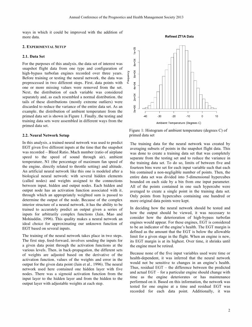
For the purposes of this analysis, the data set of interest was snapshot flight data from one type and configuration of high-bypass turbofan engines recorded over three years. Before training or testing the neural network, the data was preprocessed in two different steps. First, data points with one or more missing values were removed from the set. Next, the distribution of each variable was considered separately and, as each resembled a normal distribution, the tails of these distributions (mostly extreme outliers) were discarded to reduce the variance of the entire data set. As an example, the distribution of ambient temperature from the primed data set is shown in Figure 1. Finally, the testing and training data sets were assembled in different ways from the primed data set.

2.2. Neural Network Setup

In this analysis, a trained neural network was used to predict EGT given five different inputs at the time that the snapshot was recorded – Bleed Ratio, Mach number (ratio of airplane speed to the speed of sound through air), ambient temperature, N1 (the percentage of maximum fan speed of the engine, directly related to throttle setting) and altitude. An artificial neural network like this one is modeled after a biological neural network: with several hidden elements (called nodes) and weights assigned to the connections between input, hidden and output nodes. Each hidden and output node has an activation function associated with it, through which an appropriately weighted sum is passed to determine the output of the node. Because of the complex interior structure of a neural network, it has the ability to be trained to accurately predict an output given a series of inputs for arbitrarily complex functions (Jain, Mao and Mohiuddin, 1996). This quality makes a neural network an ideal choice for approximating our unknown function of EGT based on several inputs.

The training of the neural network takes place in two steps. The first step, feed-forward, involves sending the inputs for a given data point through the activation functions at the various levels. Then, in back-propagation, the different sets of weights are adjusted based on the derivative of the activation function, values of the weights and error in the output for the given data point (Jain et al., 1996). The neural network used here contained one hidden layer with five nodes. There was a sigmoid activation function from the input layer to the hidden layer and from the hidden to the output layer with adjustable weights at each step.

The training data for the neural network was created by averaging subsets of points in the snapshot flight data. This was done to create a training data set that was completely separate from the testing set and to reduce the variance in the training data set. To do so, limits of between five and fourteen bins were set for each input variable such that each bin contained a non-negligible number of points. Then, the entire data set was divided into 5-dimensional hypercubes bounded on each side by a bin from one input parameter. All of the points contained in one such hypercube were averaged to create a single point in the training data set. Only points from hypercubes containing one hundred or more original data points were kept.

In deciding how the neural network should be tested and how the output should be viewed, it was necessary to consider how the deterioration of high-bypass turbofan engines would appear. For these engines, EGT is considered to be an indicator of the engine’s health. The EGT margin is defined as the amount that the EGT is below the allowable limit for a given stage in the flight. When an engine is new, its EGT margin is at its highest. Over time, it shrinks until the engine must be retired.

Because none of the five input variables used were time or health-dependent, it was inferred that the neural network would not be sensitive to changes in an engine’s health. Thus, residual EGT – the difference between the predicted and actual EGT – for a particular engine should change with time as the engine deteriorates or has maintenance performed on it. Based on this information, the network was tested for one engine at a time and residual EGT was recorded for each data point. Additionally, it was

Figure 1: Histogram of ambient temperature (degrees C) of primed data set

Annual Conference of the Prognostics and Health Management Society 2013

3

determined that an increase in residual EGT would be equivalent to a decrease in EGT margin. Therefore, the speed at which residual EGT changes for a given engine should indicate how quickly the health of the engine deteriorates as a whole.

2.3. Regression Analysis

After collecting time-dependent residuals for a given engine, these residuals needed to be analyzed in order to pinpoint the differences between engines. The approach for such an analysis was determined by observing similarities between several graphs of residuals vs. time.

As demonstrated in one such graph in Figure 2, residual EGT tends to increase with time, as expected, until there are sudden shifts in the graph. At these points, residual EGT decreases by a few degrees Celsius before continuing to follow the same upward trend as before. These jumps downward indicated maintenance had been performed on the engine.

We decided that a regression analysis should stop at these points – not go through them – because they interrupt the trend. Once this decision was made, it remained to devise a method of finding these jumps. In the absence of maintenance data, two different strategies were used. First, groundings for an extended period of time – more than five days – were assumed to be maintenance events. Since each data point corresponds to one flight, this was a simple matter of finding all pairs of points separated by five days or more. This length of time allowed for planes to be grounded for weather or other non-maintenance reasons such as the temporary closure of an airport. Next, downward jumps in the data were detected using criteria similar to that used in

visual identification. That is, we identified times when a local max was closely followed by a local min at both the top and bottom of the band of residual EGT, giving the appearance of a downward vertical shift like those shown in Figure 2.

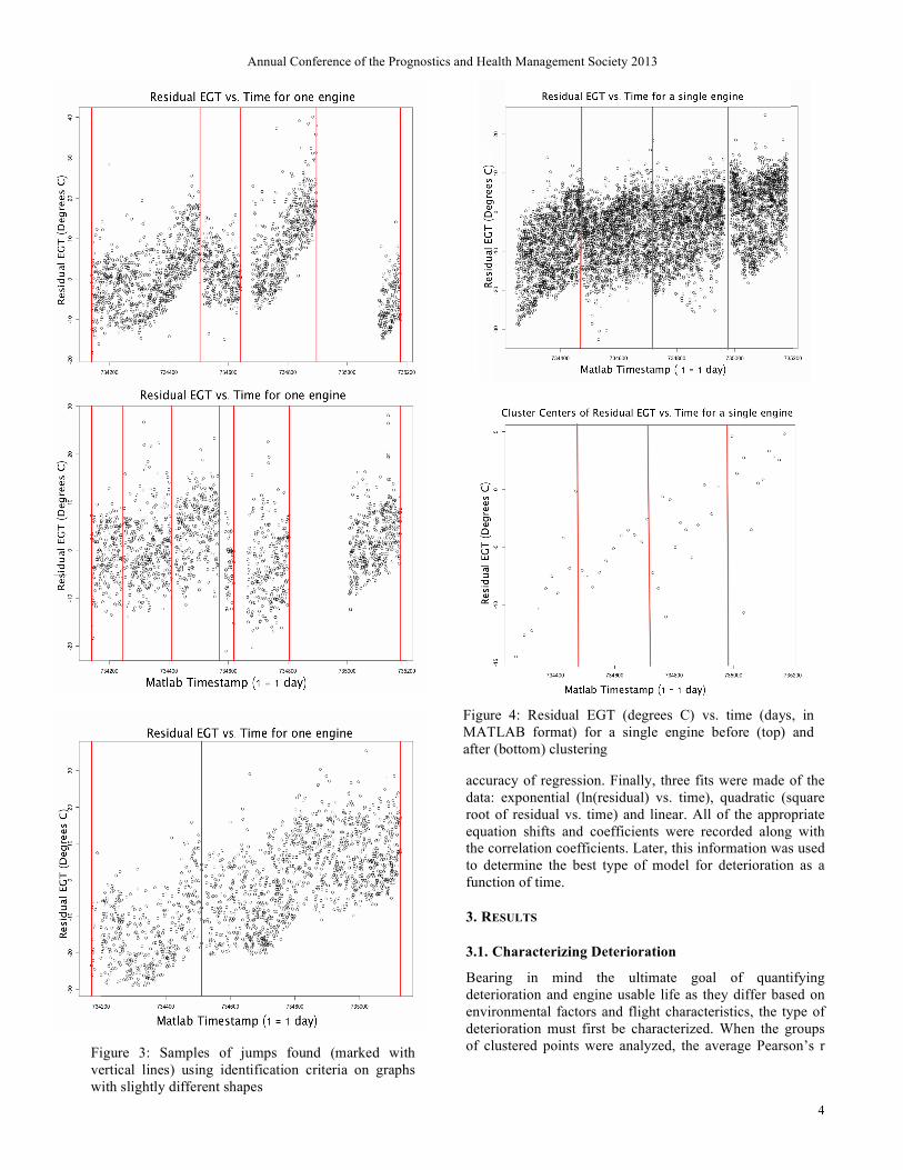
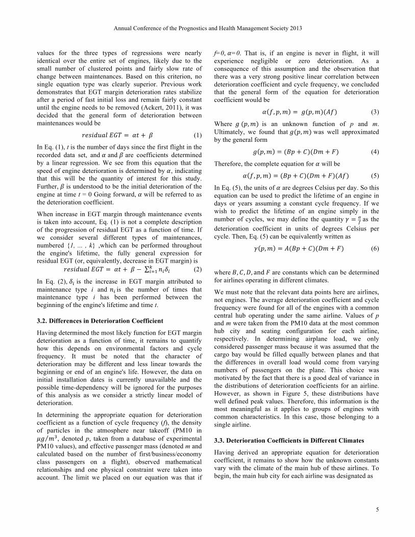
Figure 3 shows several examples of the algorithm’s success in identifying maintenance-like events. Without ground truth for maintenance event timing, the success of the jump-finding algorithm could only be judged by evaluating how often it correctly identified maintenance events compared with identification with the naked eye. Testing this method on several different graphs of residuals vs. time, we found that this method correctly identified 80 to 90 percent of the vertical discrepancies that were perceived by the naked eye to probably indicate a maintenance event. In addition, very few false positive events were identified.

Once the boundaries of the jumps were found, it remained to determine how quickly residuals changed between those boundaries. The first step in this endeavor was to cluster the data using the built-in k-means clustering algorithm (MacQueen, 1967). K-means clustering partitions a set of observations into k clusters such that the sum of the errors (distance between the cluster center and points contained in the cluster) is minimized. This is done by choosing k points, assigning each data point to the closest of those k points, and calculating the new average of each of the k sets of points. This is repeated until the centers of the clusters no longer move (MacQueen, 1967). There are many different methods that can be used to find an ideal number of clusters, k, although it has been noted that there is not necessarily a unique best value (Sugar & James, 2003) In light of this, we chose the number of clusters by performing k-means on several different time-series of residual EGT and noting how many centers would effectively cut down the noise in the data – likely due to differences in variables for which we did not account – while still demonstrating the moving trend. We found that, for this data set, approximately one center per 150 data points provides a good compromise.

An example of the effects of the k-means clustering algorithm is shown in Figure 4, which contains a plot of the original residual EGT output for a single engine, alongside the points obtained by the clustering algorithm run over the output data set. In both plots, vertical lines mark maintenance. Figure 4 shows that the resulting set of clustered points does indeed serve as a good approximation of the original data set while making performing regressions simpler. Between each set of maintenances jumps, the EGT changes in a predominantly linear fashion and the net trend is similar to those in the original data.

Next, the data was smoothed using an exponential smoothing algorithm with a small smoothing coefficient (Ostertagova & Ostertag, 2012). This technique was employed to bring potentially noisy data points just slightly closer to a perceived trend line, again to improve the

Figure 2: Residual EGT vs. Time (days, in MATLAB format) for one engine

Annual Conference of the Prognostics and Health Management Society 2013

4

accuracy of regression. Finally, three fits were made of the data: exponential (ln(residual) vs. time), quadratic (square root of residual vs. time) and linear. All of the appropriate equation shifts and coefficients were recorded along with the correlation coefficients. Later, this information was used to determine the best type of model for deterioration as a function of time.

3. RESULTS

3.1. Characterizing Deterioration

Bearing in mind the ultimate goal of quantifying deterioration and engine usable life as they differ based on environmental factors and flight characteristics, the type of deterioration must first be characterized. When the groups of clustered points were analyzed, the average Pearson’s r

Figure 4: Residual EGT (degrees C) vs. time (days, in MATLAB format) for a single engine before (top) and after (bottom) clustering

Figure 3: Samples of jumps found (marked with vertical lines) using identification criteria on graphs with slightly different shapes

Annual Conference of the Prognostics and Health Management Society 2013

5

values for the three types of regressions were nearly identical over the entire set of engines, likely due to the small number of clustered points and fairly slow rate of change between maintenances. Based on this criterion, no single equation type was clearly superior. Previous work demonstrates that EGT margin deterioration rates stabilize after a period of fast initial loss and remain fairly constant until the engine needs to be removed (Ackert, 2011), it was decided that the general form of deterioration between maintenances would be

𝑟𝑒𝑠𝑖𝑑𝑢𝑎𝑙  𝐸𝐺𝑇 =  𝛼𝑡 +  𝛽 (1)

In Eq. (1), t is the number of days since the first flight in the recorded data set, and 𝛼 and 𝛽 are coefficients determined by a linear regression. We see from this equation that the speed of engine deterioration is determined by 𝛼, indicating that this will be the quantity of interest for this study. Further, 𝛽 is understood to be the initial deterioration of the engine at time t = 0 Going forward, 𝛼 will be referred to as the deterioration coefficient.

When increase in EGT margin through maintenance events is taken into account, Eq. (1) is not a complete description of the progression of residual EGT as a function of time. If we consider several different types of maintenances, numbered {1, ... , k} ,which can be performed throughout the engine's lifetime, the fully general expression for residual EGT (or, equivalently, decrease in EGT margin) is

𝑟𝑒𝑠𝑖𝑑𝑢𝑎𝑙  𝐸𝐺𝑇 =  𝛼𝑡 +  𝛽 −   𝑛!𝛿!!!!! (2)

In Eq. (2), 𝛿! is the increase in EGT margin attributed to maintenance type i and 𝑛! is the number of times that maintenance type i has been performed between the beginning of the engine's lifetime and time t.

3.2. Differences in Deterioration Coefficient

Having determined the most likely function for EGT margin deterioration as a function of time, it remains to quantify how this depends on environmental factors and cycle frequency. It must be noted that the character of deterioration may be different and less linear towards the beginning or end of an engine's life. However, the data on initial installation dates is currently unavailable and the possible time-dependency will be ignored for the purposes of this analysis as we consider a strictly linear model of deterioration.

In determining the appropriate equation for deterioration coefficient as a function of cycle frequency (f), the density of particles in the atmosphere near takeoff (PM10 in 𝜇𝑔 𝑚!, denoted p, taken from a database of experimental PM10 values), and effective passenger mass (denoted m and calculated based on the number of first/business/economy class passengers on a flight), observed mathematical relationships and one physical constraint were taken into account. The limit we placed on our equation was that if

f=0, 𝛼=0. That is, if an engine is never in flight, it will experience negligible or zero deterioration. As a consequence of this assumption and the observation that there was a very strong positive linear correlation between deterioration coefficient and cycle frequency, we concluded that the general form of the equation for deterioration coefficient would be

𝛼 𝑓, 𝑝,𝑚 =  𝑔(𝑝,𝑚)(𝐴𝑓) (3)

Where 𝑔  (𝑝,𝑚) is an unknown function of p and m. Ultimately, we found that 𝑔(𝑝,𝑚) was well approximated by the general form

𝑔 𝑝,𝑚 = (𝐵𝑝 + 𝐶)(𝐷𝑚 + 𝐹) (4)

Therefore, the complete equation for 𝛼 will be

𝛼 𝑓, 𝑝,𝑚 = (𝐵𝑝 + 𝐶)(𝐷𝑚 + 𝐹)(𝐴𝑓) (5)

In Eq. (5), the units of 𝛼 are degrees Celsius per day. So this equation can be used to predict the lifetime of an engine in days or years assuming a constant cycle frequency. If we wish to predict the lifetime of an engine simply in the number of cycles, we may define the quantity 𝛾 = !

! as the deterioration coefficient in units of degrees Celsius per cycle. Then, Eq. (5) can be equivalently written as

𝛾 𝑝,𝑚 = 𝐴(𝐵𝑝 + 𝐶)(𝐷𝑚 + 𝐹) (6)

where  𝐵,𝐶,𝐷, and  𝐹 are constants which can be determined for airlines operating in different climates.

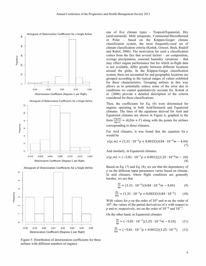
We must note that the relevant data points here are airlines, not engines. The average deterioration coefficient and cycle frequency were found for all of the engines with a common central hub operating under the same airline. Values of p and m were taken from the PM10 data at the most common hub city and seating configuration for each airline, respectively. In determining airplane load, we only considered passenger mass because it was assumed that the cargo bay would be filled equally between planes and that the differences in overall load would come from varying numbers of passengers on the plane. This choice was motivated by the fact that there is a good deal of variance in the distributions of deterioration coefficients for an airline. However, as shown in Figure 5, these distributions have well defined peak values. Therefore, this information is the most meaningful as it applies to groups of engines with common characteristics. In this case, those belonging to a single airline.

3.3. Deterioration Coefficients in Different Climates

Having derived an appropriate equation for deterioration coefficient, it remains to show how the unknown constants vary with the climate of the main hub of these airlines. To begin, the main hub city for each airline was designated as

Annual Conference of the Prognostics and Health Management Society 2013

6

one of five climate types - Tropical/Equatorial, Dry (arid/semiarid), Mild temperate, Continental/Microthermal or Polar – based on the Köppen-Geiger climate classification system, the most frequently-used set of climate classification criteria (Kottek, Grieser, Beck, Rudolf and Rubel, 2006). The motivation for such a classification comes from the fact that several factors – air composition, average precipitation, seasonal humidity variations – that may effect engine performance but for which in-flight data is not available, differ greatly between different locations around the globe. In the Köppen-Geiger classification system, these are accounted for and geographic locations are grouped according to the typical ranges of values exhibited for these characteristics. Grouping airlines in this way allows us to potentially reduce some of the error due to conditions we cannot quantitatively account for. Kottek et al. (2006) provide a detailed description of the criteria considered for these classifications.

Then, the coefficients for Eq. (6) were determined for engines operating in both Arid/Semiarid and Equatorial climates. The lines of the equations derived for Arid and Equatorial climates are shown in Figure 6, graphed in the form ! !,!

!"!!= 𝐴(𝐷𝑚 + 𝐹) along with the points for airlines

corresponding to those climates.

For Arid climates, it was found that the equation for 𝛾 would be

𝛾 𝑝,𝑚 = (1.31 ∙ 10!!𝑝 + 0.0033)(4.84 ∙ 10!!𝑚 − 4.44) (7)

And similarly, in Equatorial climates,

𝛾 𝑝,𝑚 = (−5.81 ∙ 10!!𝑝 + 0.0012)(1.25 ∙ 10!!𝑚 − .10) (8)

Based on Eq. (7) and Eq. (8), we see that the dependency of 𝛾 on the different input parameters varies based on climate. In arid climates, where flight conditions are generally harsher, we see that

!"!"= (1.31 ∙ 10!!)(4.84 ∙ 10!!𝑚 − 4.44) (9)

!"!"

= 1.31 ∙ 10!!𝑝 + 0.0033 4.84 ∙ 10!! (10)

With values for p on the order of 10! and m on the order of 10!, the values of the partial derivatives of 𝛾 with respect to p and m, respectively, are on the order of 10!! and 10!!.

On the other hand, in Equatorial climates !"!"= (−5.81 ∙ 10!!)(1.25 ∙ 10!!𝑚 − 0.10) (11)

!"!"

= (−5.81 ∙ 10!!𝑝 + 0.0012)(1.25 ∙ 10!!) (12)

Figure 5: Distribution of deterioration coefficients for three airlines with different numbers of engines

Annual Conference of the Prognostics and Health Management Society 2013

7

Using the same estimates for p and m, we see that the values of the partial derivatives of 𝛾 with respect to p and m, respectively, are on the order of 10!! and 10!! , almost negligible compared with those in Arid climates. So we see that in less harsh climates, deterioration coefficient is much less sensitive to changes in flight conditions.

4. DISCUSSION AND CONCLUSION

We see in Figure 5 that although this model of deterioration coefficient is fairly accurate, it is not perfect. Here, we ignored several possible parameters that could have affected deterioration coefficient, possibly bringing the points in Figure 5 closer to the trend line and creating a slightly better model. This was motivated both by a desire to keep the model from becoming too complicated to be useful and an absence of reliable data. A few such parameters would have been runway length or fuel efficiency - indicators of how the plane is flown differently between airlines. However, we also note that these factors may be difficult to define before the engine is put into service, making an accurate prediction of deterioration coefficient with a refined model difficult.

Despite the possibility that this model is not a perfect description of deterioration coefficient, we are now equipped with a tool that can be used to help manufacturers and users of high-bypass turbofan engines with reasonable accuracy.

First and foremost, our model allows us to make estimates on the relative lifetimes of engines under different conditions. Using the specific value of 𝛼 or, equivalently, 𝛾 for a given airline, along with a pre-specified maintenance plan and initial EGT margin, we can use Eq. (2) to predict either the number of days or cycles that an engine will last on the wing of a plane. Both airlines and engine manufacturers can use this information to determine how often an engine needs to be maintained for it to reach a desired number of cycles or years of use.

Once lifetime estimates and maintenance patterns are determined for a specific engine, this information can be used in financial considerations for producers and consumers. Companies that produce or maintenance engines, knowing what the maintenance frequency will likely be, can use this information to determine how much maintenance events should cost to appropriately offset the price of producing the engine. Airlines can use this model and the resulting recommended maintenance patterns in a similar way. Knowing how much an airline will need to spend on an engine (or a set of engines in a fleet) during its usable life will allow ticket prices to be adjusted accordingly.

We see here that this model has the potential to help save both time and resources. The major shortfall of this study is that it only included a few airlines per climate type, some of which did not have data on very many engines, and that

only two different climate types were considered. At the time of the study, all of the available data was used. However, with more flight data from a wider array of engine models, configurations, locations and airlines, the analysis performed here could be expanded, making it more accurate and robust.

REFERENCES

Ackert, S. (2011). Engine Maintenance Concepts for Financiers: Elements of Turbofan Shop Maintenance Costs. Aircraft Monitor. http://www.aircraftmonitor.com/uploads/1/5/9/9/15993320/engine_mx_concepts_for_financiers___v2.pdf

Changzheng, L., Yong, L. (2006). Fault Diagnosis for an Airgraft Engine Based on Information Fusion. IEEE 3rd International Conference on Mechatronics (199-202)

Jain, A.K., Mao, J., Mohiuddin, K.M. (1996) Artificial

Figure 6: Functions of deterioration coefficient graphed with points for different airlines operating in Equatorial (top) and Arid (bottom) climates

Annual Conference of the Prognostics and Health Management Society 2013

8

Neural Networks: A Tutorial. IEEE Computer 29, 31-44. http://www4.rgu.ac.uk/files/chapter3%20-%20bp.pdf

Kottek, M., Grieser, J., Beck, C., Rudolf, B., Rubel, F. (2006). World Map of the Köppen-Geiger Climate Classifiation Updated. Meteorologische Zeitschrift. 15 (6), 259-263.

Krok, M.J., Ashby, M.J. (2002). Condition-based, Diagnostic Gas Path Reasoning for Gas Turbine Engines. 2002 IEEE lntemational Conference on Control Applications. September 18-20. Glasgow, Scotland,U.K.

MacQueen, J. (1967). Some methods for classification and analysis of multivariate observations. In Proceedings of the Berkeley Symposium on Mathematical Statistics and Probability, 281-297. Berkeley, CA, USA

Ostertagova, E.,Ostertag, O. (2012). Forecasting using simple exponential smoothing method. Acta Electrotechnica et Informatica 12 (3), 62-66. DOI: 10.2478/v10198-012-0034-2

Saxena, A., Goebel, K., Simon, D., Eklund, N., (2008). Damage Propagation Modeling for Aircraft Engine Run-to-Failure Simulation. International Conference on Prognostics and Health Management, 2008. pp. 1–9. IEEE.

Sugar, C.A., James, G.M. (2003). Finding the number of clusters in a data set: An information theoretic approach. Journal of the American Statistical Association. 98 (463). pp. 750-763. DOI: 10.1198/016214503000000666

Weizhong, Y., Feng, X. (2008). Jet Engine Gas Path Fault Diagnosis Using Dynamic Fusion of Multiple Classifiers. 2008 International Joint Conference on Neural Networks (1585-1591).

BIOGRAPHIES

Christina Brasco is currently an undergraduate at Yale University and will receive her B.S. in Physics and Mathematics in 2014. She worked as a Data Science CoE intern at General Electric’s Software Center of Excellence in the summer of 2013. During the summers of 2012 and 2011, she worked as an undergraduate research assistant on the MicroBooNE Collaboration. She won Yale’s Benjamin F. Barge Prize for the solution of original problems in mathematics in 2011 and was a member of the 2010 U.S. Physics Team.

Neil H. W. Eklund, Ph.D. had been a research scientist in the Machine Learning Laboratory of General Electric Global Research since 2002. He has worked on a wide variety of research projects related to remote monitoring, diagnostics, and prognostics for military and commercial aircraft engines, medical devices, wind turbines, manufacturing systems, ground-based gas turbines, and other platforms. He holds eight patents, with another eight pending, and has authored over 70 technical publications.

Neil is also an Adjunct Professor of Electrical Engineering and Computer Science at Union Graduate College in Schenectady, NY since 2005. He was one of the co-founders of the PHM Society, the first Editor-in-Chief of the International Journal of Prognostics and Health Management (ijPHM) from 2009-2011, and is active in the organization of the annual PHM Society conference. He also works with the ISO to develop standards related to diagnostics and prognostics. Mohak Shah, Ph.D. is a research scientist at GE Global Research. He is the co-author of "Evaluating Learning Algorithms: A Classification Perspective" published by Cambridge University Press. His research interests span machine learning, statistical learning theory and their application to a variety of domains. More details can be found at: http://www.mohakshah.com Daniel E. Marthaler, Ph.D. has been a Senior research scientist in the Industrial Internet Analytics Laboratory of General Electric's Software Center of Excellence since May 2012. He holds a PhD in Mathematics from Arizona State University and has been working on problems in the realm of Artificial Intelligence and applied Machine Learning for over a decade. He has over 25 peer reviewed publications and has authored the Gaussian Process in Machine Learning (GPML) toolkit in Python.