European Journal of Soil Science, May 2015, 66, 535–547 doi: 10.1111/ejss.12244
Predictive soil mapping with limited sample data
A . X . Z h u a,b,c,d, J . L i u d, F . D u d, S . J . Z h a n g c, C . Z . Q i n c, J . B u r t d, T . B e h r e n s e &T . S c h o l t e n e
aSchool of Geography Science, Nanjing Normal University, 1 Wenyuan Road, Nanjing 210023, China, bJiangsu Center for CollaborativeInnovation in Geographical Information Resource Development and Application, 1 Wenyuan Road, Nanjing 210023, China, cState KeyLaboratory of Resources and Environmental Information System, Institute of Geographical Sciences and Natural Resources Research,Chinese Academy of Sciences, 11A Datun Road, Beijing 100101, China, dDepartment of Geography, University of Wisconsin - Madison,550 North Park Street, Madison, Wisconsin 53706, USA, and eInstitute of Geography, Physical Geography, University of Tübingen,Rümelinstraße 19-23, D-72074 Tübingen, Germany
Summary
Existing predictive soil mapping (PSM) methods often require soil sample data to be sufficient to representsoil–environment relationships throughout the study area. However, in many parts of the world with only alimited quantity of soil sample data to represent the study area, this is still an issue for PSM application. Thispaper presents a method, named ‘individual predictive soil mapping’ (iPSM), which can make use of limited soilsample data for PSM. With the assumption that similar environmental conditions have similar soils, iPSM usesthe soil–environment relationship at each individual soil sample location to predict soil properties at unvisitedlocations and estimate prediction uncertainty. Specifically, the environmental similarities of an unvisited locationto a set of soil sample locations are used in a weighted average method to integrate the soil–environmentrelationships at sample locations for prediction and uncertainty estimation. As a case study, iPSM was appliedto map soil organic matter (SOM) content (%) in the topsoil layer using two sets of soil samples. Comparedwith multiple linear regression (MLR), iPSM produced a more accurate SOM map (root mean squared error(RMSE) 1.43, mean absolute error (MAE) 1.16) than MLR (RMSE 8.54, MAE 7.34) the ability of the sampleset to represent the study area is limited and achieved a comparable accuracy (RMSE 1.10, MAE 0.69) withMLR (RMSE 1.01, MAE 0.73) when the sample set could represent the study area better. In addition, theprediction uncertainty estimated by iPSM was positively related to prediction residuals in both scenarios. Thisstudy demonstrates that iPSM is an effective alternative when existing soil samples are limited in their abilityto represent the study area and the prediction uncertainty in iPSM can be used as an indicator of its predictionaccuracy.
Introduction
Soil sample data are often used for calibrating or constructinga predictive soil mapping (PSM) model (McBratney et al., 2003;Scull et al., 2003; Zhu et al., 2010). Generally, it is required that thesample data should be sufficient to represent the soil–environmentrelationships throughout a study area for reliable model calibrationor construction (Ramsey & Hewitt, 2005). From probability theoryand geostatistical analysis, sufficient soil sample data usually needto be collected through a well-defined field sampling design, whichtypically aims to allocate soil samples in geographical space and/orenvironmental covariate space (feature space) in such a way thatthe designed sample set is representative of the area (Webster &
Received 12 June 2014; revised version accepted 20 January 2015
Oliver, 1990; van Groenigen & Stein, 1998; de Gruijter et al.,2006; Minasny & McBratney, 2006; Zhu et al., 2008). The fuzzylogic-based techniques (Zhu, 1999, 2001; Qi & Zhu, 2003) alsorequire that the knowledge or the soil sample set needs to berepresentative of the area for reliable construction of the fuzzymembership function.
In practice, however, it can be difficult to collect a set of soilsamples that is sufficiently representative of the study area. Becauseof the costs of field sampling and laboratory analysis, the numberof soil sample points actually collected can be limited. In addition,positioning errors can result in the mismatch between the actualand the design locations, and the limited expertise of soil surveyorscan also cause bias in the collected samples (Johnson et al., 2012).Those constraints can easily lead to the collected soil sampleset not being representative of the soil-environment relationshipsthroughout the study area.
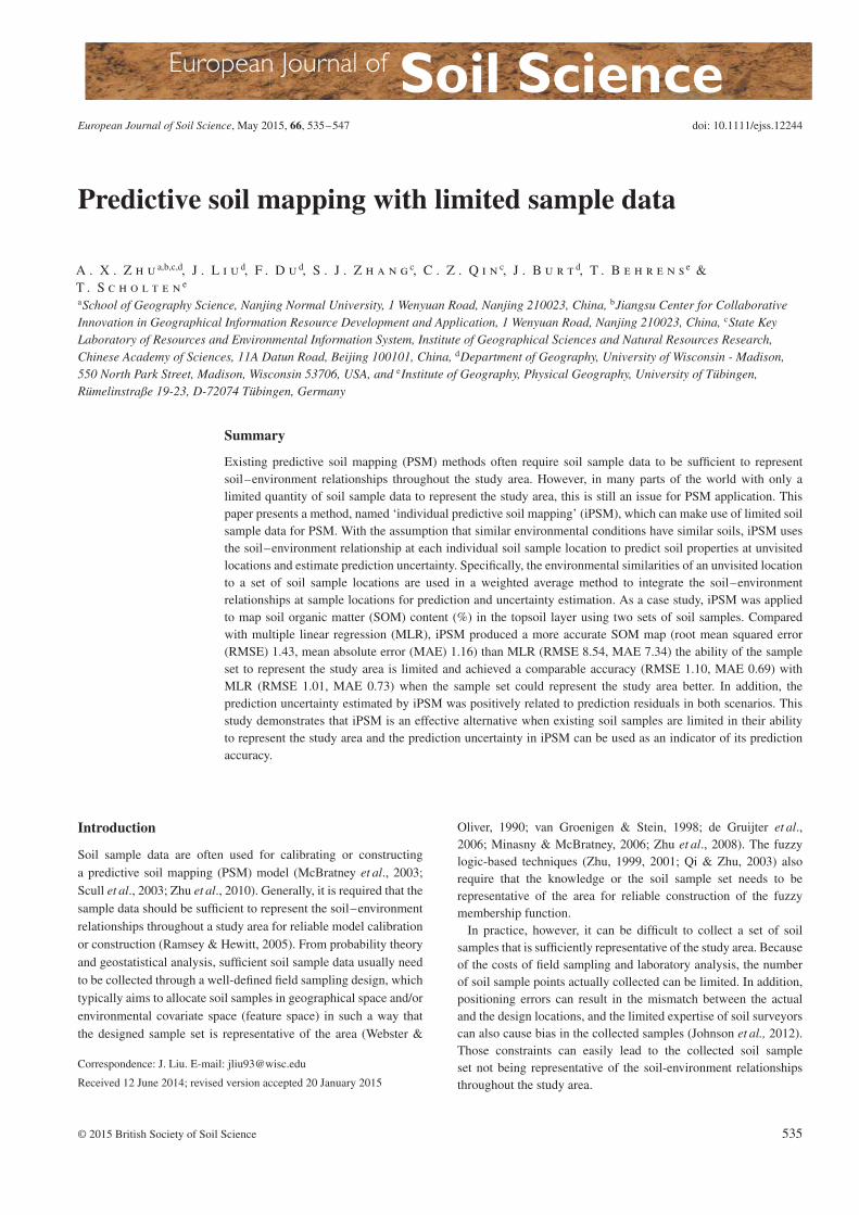
Figure 1 The flowchart of the individual predictive soil mapping (iPSM) method.
The problem of limited soil sample data, which are not adequateto represent soil–environment relationships in a study area, presentschallenges for existing PSM methods. One problem is that is thedata are not sufficient for developing a reliable soil–environmentmodel with existing PSM methods (such as regression and kriging).As a consequence, the estimation of prediction uncertainty usingexisting methods, such as the error variance in kriging method,may not be valid.
This paper presents a PSM method, called ‘individual predictivesoil mapping’ (iPSM), which is capable of using limited soilsample data for predictive soil mapping and quantifying predictionuncertainty. The next section of this paper presents the method-ologies of iPSM in detail. Then we apply iPSM in a case study formapping the content of soil organic matter (SOM, %) in the topsoillayer and quantifying prediction uncertainty and compare this withmultiple linear regression (MLR). We use two soil sample datasets:one has limitations in representing the study area and the other canrepresent it better.
Methods
Basic idea and overall design
Soil samples, however limited their ability to represent soil–environment relationships in a study area, still contain valuableinformation for PSM. For example, each individual soil samplepoint reflects the in situ relationship of soil to the environmental‘niche’ that it is in. By assuming that locations with similar envi-ronmental conditions have similar soil properties (Hudson, 1992;Mallavan et al., 2010), similar values of the targeted soil propertycan be expected at locations with similar environmental conditions.Therefore, each soil sample point can individually serve as asurrogate representing the locations with similar environmentalconditions, and thus can be used to predict the soil conditions forthese locations.
The overall design of iPSM contains three major steps (Figure 1):(i) the characterization of environmental conditions at each location,(ii) the assessment of environmental similarities at every unvisited
location and every soil sample location and (iii) the estimation ofthe value of the targeted soil property and the quantification ofprediction uncertainty at each location.
Characterization of environmental conditions
Environmental conditions associated with soil at each location needto be quantitatively characterized. It is important to use the environ-mental variables (the environmental covariates) that are effectivein indicating the spatial variation of a targeted soil property in agiven study area. According to the state equation of soil formation(Jenny, 1941), there are five environmental state factors (climate,parent material, topography, biology and time) that need to be con-sidered. Each environmental state factor can be characterized byusing various environmental variables (or covariates) (McBratneyet al., 2003). The selection of an appropriate environmental covari-ate depends on its (i) ability to indicate the spatial variation of atargeted soil property and (ii) availability regarding data sources.Commonly used environmental covariates include annual averagedtemperature, annual averaged precipitation, parent materials, eleva-tion, slope aspect, slope gradient, profile and planform curvatures,topographic wetness index, distance to streams, land use and coverand vegetation index (McBratney et al., 2003; Florinsky, 2011).The advances in earth observation technologies and spatial analy-sis methods have also provided many new candidate environmentalcovariates (Mendonça-Santos et al., 2006; Kienast-Brown & Boet-tinger, 2007; Nield et al., 2007; Zhu et al., 2010; Liu et al., 2012).Usually, multiple environmental covariates are needed to character-ize the environmental conditions related to the targeted soil prop-erties. At a given location an environmental vector is formed tocharacterize the environmental conditions:
e =(e1, e2, … , em
), (1)
where m is the number of environmental covariates used.
Assessment of environmental similarity
From the environmental vector, the environmental similaritybetween an unvisited location i (i= 1, 2, 3, … ,k; k is the numberof locations to be predicted, typically grid cells) and a soil samplepoint j (j= 1,2,3,… , n; n is the number of available soil samplepoints) needs to be determined at the scale(s) of the environmentalcovariate and soil sample (Shi et al., 2004):
Si,j = P(E(e1i, e1j
),E
(e2i, e2j
), … ,E
(evi, evj
), … ,E
(emi, emj
)),
(2)where Si,j represents the environmental similarity between unvisitedlocation i and sample location j, evi and evj are the values of thevth environmental covariate at the two locations, and E(•) andP(•) are functions for calculating environmental similarity at theenvironmental covariate scale and soil sample scale, which areexplained next.
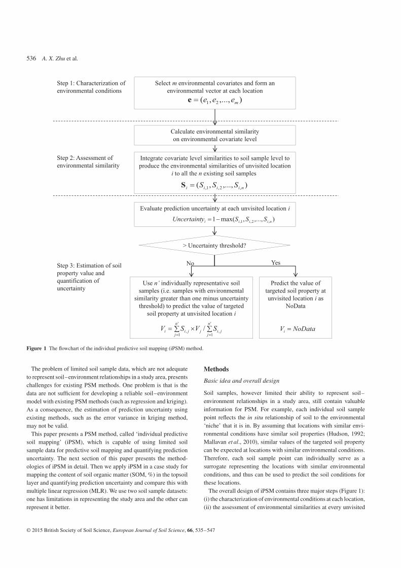
Function E(•) is for calculating environmental similarity at theenvironmental covariate scale. Given an environmental covariate,E(•) describes how the environmental similarity between an unvis-ited location and a sample location changes when the value of theenvironmental covariate at the unvisited location deviates from thevalue at the sample location. For iPSM, we define E(•) depend-ing on the measurement scale (Stevens, 1946) of the environmentalcovariate:
E(evi, evj
)=
⎧⎪⎪⎪⎪⎪⎨⎪⎪⎪⎪⎪⎩
0 ev is nominal∕ordinal and evi ≠ evj
1 ev is nominal∕ordinal and evi = evj
exp
⎛⎜⎜⎜⎝−(evi−evj)2
2
(SDev×
SDevSDevj
)2
⎞⎟⎟⎟⎠ v is interval∕ratio
,
(3)in which SDev
is the standard deviation of the vth environmentalcovariate in the study area, and SDevj
is the square root of the meandeviation of the values of the vth environmental covariate at allunvisited locations (i= 1, 2, … , k) from that at sample locationj (i.e. evj):
SDevj=
√√√√√√ k∑i=1
(evi − evj
)2
k. (4)
According to Equation (3), if the covariate has been recorded ona nominal or ordinal scale, such as parent material type, a steppedE(•) will be used (Figure 2a). This E(•) produces a value of 1 whenthe value of the covariate at an unvisited location is the same as thatat a sample location and 0 otherwise. For environmental covariatesmeasure on interval or ratio scales such as precipitation or elevationa Gaussian-shaped E(•) is designed to determine the similarity(Figure 2b). The width of the Gaussian-shaped curve, which iscontrolled by the standard deviation of the vth environmentalcovariate (SDev
), is further adjusted by SDevj(Equation (4)). This
adjustment leads to a Gaussian-shaped curve that is spread overthe range of the vth environmental covariate when the value at thesoil sample location j is similar to many other prediction locations(therefore, smaller SDevj
) and vice versa. The aim of adjusting thewidth of the curve is to differentiate soil sample points that representa common soil-environment relationship in the study area from soilsample points that represent a rare soil-environment relationship inthe study area.
Function P(•) is used to integrate environmental similarities forcovariates with those for soil samples. The form of P(•) shouldtake into consideration the relative importance of multiple types ofenvironmental covariates in influencing the value of the targeted soilproperty. The choices of P(•) include weighted average methods,which require the relative weights for every environmental covariate(McBratney et al., 2003), decision trees, which allow a hierarchyconfiguration of the relative importance (Mallavan et al., 2010), and
Figure 2 The E function used for estimatingenvironmental similarity at the environmentalcovariate scale: (a) when the environmentalcovariate is nominal or ordinal; (b) when the envi-ronmental covariate is interval or ratio.
a minimum operator based on the Liebig’s law of the minimum (vander Ploeg et al., 1999). In our paper, a minimum operator was used:the smallest value among all environmental covariate similaritieswas used as the environmental similarity at the soil sample level(Zhu et al., 1997; Shi et al., 2004).
The outputs from the assessment of environmental similarity to allexisting soil sample points were organized into a similarity vectorat each unvisited location i:
Si =(Si,1, Si,2, … , Si,n
), (5)
in which Siis the vector containing environmental similaritiesbetween unvisited location i and the n soil samples.
Quantification of prediction uncertainty and estimation of soilproperty value
Prediction uncertainty at each location is inversely related to itsenvironmental similarities to the existing soil samples. The rationalefor this is that if the similarities in environmental conditionsbetween the unvisited location and the sample points used are poor,then the existing sample points cannot be used to represent thatlocation. Thus, the use of these samples to predict the soil conditionsat that location would lead to much uncertainty. Therefore, theuncertainty measurement in iPSM is basically a measurement ofhow reliable it is to use existing soil sample points to represent agiven unvisited location for prediction. It is given as the followingequation:
Uncertaintyi = 1 − max(Si,1, Si,2, … , Si,n
). (6)
Equation (6) indicates that prediction uncertainty is expected to belarge at unvisited location i when none of the n soil sample pointsis environmentally similar to this location.
It is necessary to examine whether an unvisited location can bepredicted by existing soil samples with an acceptable uncertainty. Auser-defined uncertainty threshold is set for this purpose. For a loca-tion whose prediction uncertainty is greater than this uncertainty
threshold, the value of a targeted soil property at the location is setto ‘NoData’ to indicate that prediction at this location using existingsoil samples cannot be made with an acceptable range of uncer-tainty. The choice of uncertainty threshold depends on the user’stolerance regarding the reliability of using existing soil samples torepresent the unvisited location. A strict uncertainty threshold suchas a small value means that the user is required to use the existingsoil samples to predict only the unvisited locations with very similarenvironmental conditions.
For a location whose prediction uncertainty does not exceed thethreshold, the value of the target property at this location is predictedfrom the soil samples whose environmental similarity exceeds thevalue of one less the uncertainty threshold. In other words, onlythose soil samples that are similar enough to the unvisited locationare used to compute the value of the targeted property at that site.The estimation of the value of the targeted soil property is calculatedwith a weighted average method (Zhu et al., 1997):
Vi =∑n′
j=1 Si,j × Vj∑n′
j=1 Si,j
, (7)
in which n′ is the number of the selected soil samples whoseenvironmental similarity to the unvisited location i exceeds oneminus the uncertainty threshold, Si,j is the environmental similarityof the unvisited location i to the soil sample location j, and Vj is thevalue of the targeted soil property of soil sample at location j.
Case study
Study area and datasets
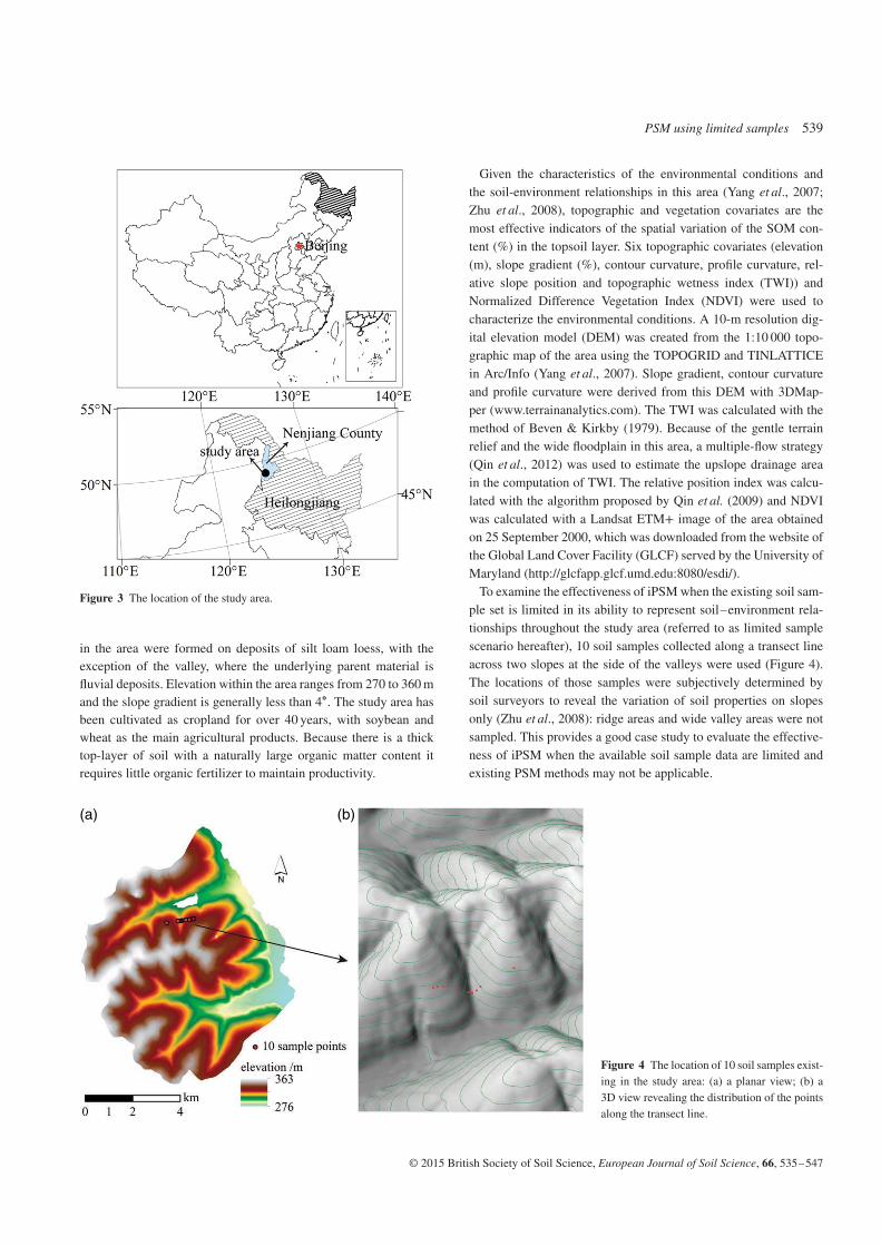
To test the effectiveness, iPSM was used for predicting soil organicmatter (SOM) content (%) in the topsoil layer of an area ofapproximately 60 km2. The study area is located in Heshan Farm,Nenjiang County, Heilongjiang Province of China (Figure 3).The annual temperature ranges from −38 to 36∘C, the ≥10∘Caccumulated temperature over one year is about 2000–2300∘C,and the average annual precipitation is 500–600 mm. Most soils
in the area were formed on deposits of silt loam loess, with theexception of the valley, where the underlying parent material isfluvial deposits. Elevation within the area ranges from 270 to 360 mand the slope gradient is generally less than 4∘. The study area hasbeen cultivated as cropland for over 40 years, with soybean andwheat as the main agricultural products. Because there is a thicktop-layer of soil with a naturally large organic matter content itrequires little organic fertilizer to maintain productivity.
Given the characteristics of the environmental conditions andthe soil-environment relationships in this area (Yang et al., 2007;Zhu et al., 2008), topographic and vegetation covariates are themost effective indicators of the spatial variation of the SOM con-tent (%) in the topsoil layer. Six topographic covariates (elevation(m), slope gradient (%), contour curvature, profile curvature, rel-ative slope position and topographic wetness index (TWI)) andNormalized Difference Vegetation Index (NDVI) were used tocharacterize the environmental conditions. A 10-m resolution dig-ital elevation model (DEM) was created from the 1:10 000 topo-graphic map of the area using the TOPOGRID and TINLATTICEin Arc/Info (Yang et al., 2007). Slope gradient, contour curvatureand profile curvature were derived from this DEM with 3DMap-per (www.terrainanalytics.com). The TWI was calculated with themethod of Beven & Kirkby (1979). Because of the gentle terrainrelief and the wide floodplain in this area, a multiple-flow strategy(Qin et al., 2012) was used to estimate the upslope drainage areain the computation of TWI. The relative position index was calcu-lated with the algorithm proposed by Qin et al. (2009) and NDVIwas calculated with a Landsat ETM+ image of the area obtainedon 25 September 2000, which was downloaded from the website ofthe Global Land Cover Facility (GLCF) served by the University ofMaryland (http://glcfapp.glcf.umd.edu:8080/esdi/).
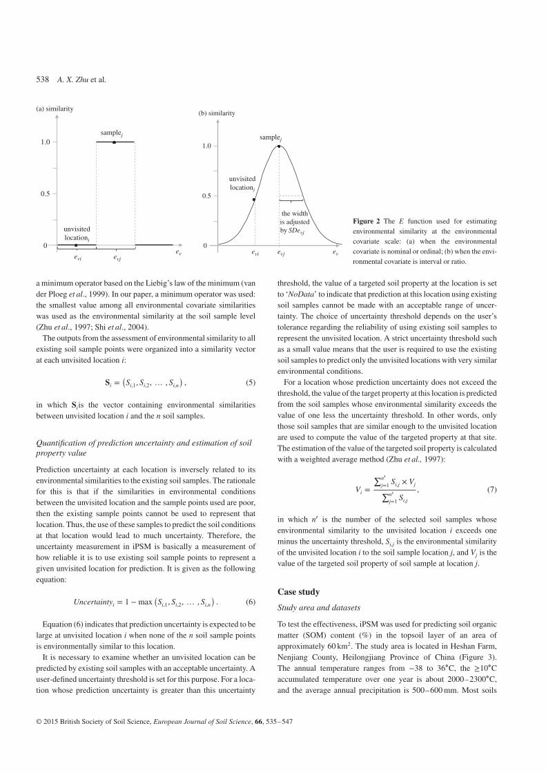
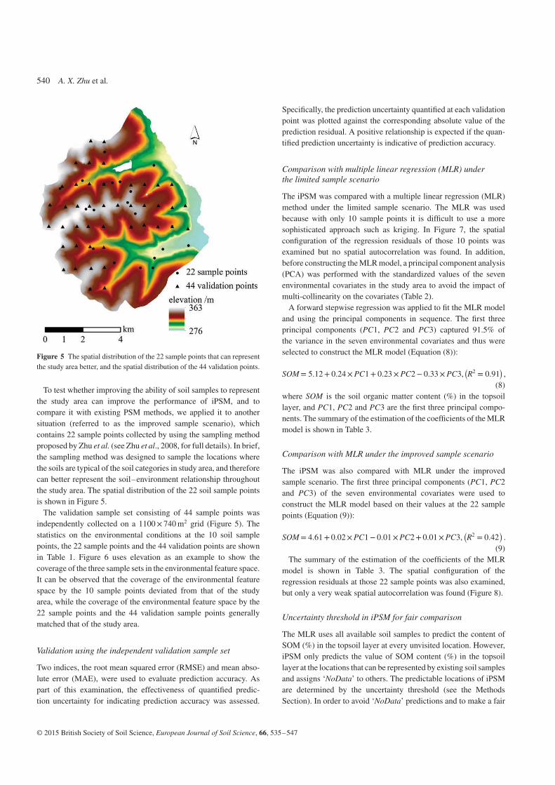
To examine the effectiveness of iPSM when the existing soil sam-ple set is limited in its ability to represent soil–environment rela-tionships throughout the study area (referred to as limited samplescenario hereafter), 10 soil samples collected along a transect lineacross two slopes at the side of the valleys were used (Figure 4).The locations of those samples were subjectively determined bysoil surveyors to reveal the variation of soil properties on slopesonly (Zhu et al., 2008): ridge areas and wide valley areas were notsampled. This provides a good case study to evaluate the effective-ness of iPSM when the available soil sample data are limited andexisting PSM methods may not be applicable.
(a) (b)
Figure 4 The location of 10 soil samples exist-ing in the study area: (a) a planar view; (b) a3D view revealing the distribution of the pointsalong the transect line.
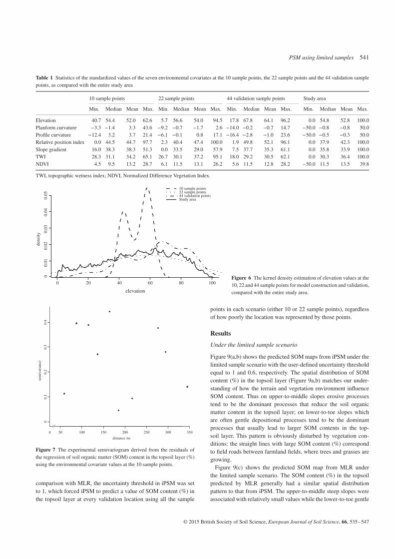
Figure 5 The spatial distribution of the 22 sample points that can representthe study area better, and the spatial distribution of the 44 validation points.
To test whether improving the ability of soil samples to representthe study area can improve the performance of iPSM, and tocompare it with existing PSM methods, we applied it to anothersituation (referred to as the improved sample scenario), whichcontains 22 sample points collected by using the sampling methodproposed by Zhu et al. (see Zhu et al., 2008, for full details). In brief,the sampling method was designed to sample the locations wherethe soils are typical of the soil categories in study area, and thereforecan better represent the soil–environment relationship throughoutthe study area. The spatial distribution of the 22 soil sample pointsis shown in Figure 5.
The validation sample set consisting of 44 sample points wasindependently collected on a 1100× 740 m2 grid (Figure 5). Thestatistics on the environmental conditions at the 10 soil samplepoints, the 22 sample points and the 44 validation points are shownin Table 1. Figure 6 uses elevation as an example to show thecoverage of the three sample sets in the environmental feature space.It can be observed that the coverage of the environmental featurespace by the 10 sample points deviated from that of the studyarea, while the coverage of the environmental feature space by the22 sample points and the 44 validation sample points generallymatched that of the study area.
Validation using the independent validation sample set
Two indices, the root mean squared error (RMSE) and mean abso-lute error (MAE), were used to evaluate prediction accuracy. Aspart of this examination, the effectiveness of quantified predic-tion uncertainty for indicating prediction accuracy was assessed.
Specifically, the prediction uncertainty quantified at each validationpoint was plotted against the corresponding absolute value of theprediction residual. A positive relationship is expected if the quan-tified prediction uncertainty is indicative of prediction accuracy.
Comparison with multiple linear regression (MLR) underthe limited sample scenario
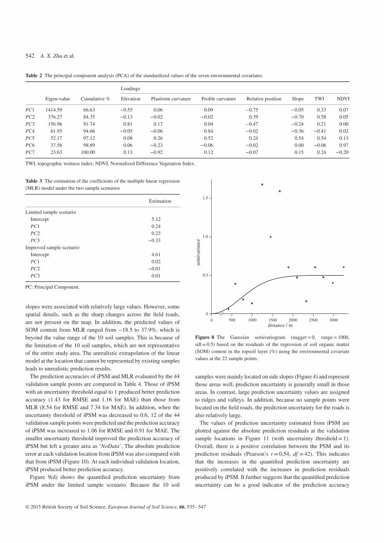
The iPSM was compared with a multiple linear regression (MLR)method under the limited sample scenario. The MLR was usedbecause with only 10 sample points it is difficult to use a moresophisticated approach such as kriging. In Figure 7, the spatialconfiguration of the regression residuals of those 10 points wasexamined but no spatial autocorrelation was found. In addition,before constructing the MLR model, a principal component analysis(PCA) was performed with the standardized values of the sevenenvironmental covariates in the study area to avoid the impact ofmulti-collinearity on the covariates (Table 2).
A forward stepwise regression was applied to fit the MLR modeland using the principal components in sequence. The first threeprincipal components (PC1, PC2 and PC3) captured 91.5% ofthe variance in the seven environmental covariates and thus wereselected to construct the MLR model (Equation (8)):
(8)where SOM is the soil organic matter content (%) in the topsoillayer, and PC1, PC2 and PC3 are the first three principal compo-nents. The summary of the estimation of the coefficients of the MLRmodel is shown in Table 3.
Comparison with MLR under the improved sample scenario
The iPSM was also compared with MLR under the improvedsample scenario. The first three principal components (PC1, PC2and PC3) of the seven environmental covariates were used toconstruct the MLR model based on their values at the 22 samplepoints (Equation (9)):
(9)The summary of the estimation of the coefficients of the MLR
model is shown in Table 3. The spatial configuration of theregression residuals at those 22 sample points was also examined,but only a very weak spatial autocorrelation was found (Figure 8).
Uncertainty threshold in iPSM for fair comparison
The MLR uses all available soil samples to predict the content ofSOM (%) in the topsoil layer at every unvisited location. However,iPSM only predicts the value of SOM content (%) in the topsoillayer at the locations that can be represented by existing soil samplesand assigns ‘NoData’ to others. The predictable locations of iPSMare determined by the uncertainty threshold (see the MethodsSection). In order to avoid ‘NoData’ predictions and to make a fair
Table 1 Statistics of the standardized values of the seven environmental covariates at the 10 sample points, the 22 sample points and the 44 validation samplepoints, as compared with the entire study area
10 sample points 22 sample points 44 validation sample points Study area
Min. Median Mean Max. Min. Median Mean Max. Min. Median Mean Max. Min. Median Mean Max.
10 sample points22 sample points44 validation points Study area
Figure 6 The kernel density estimation of elevation values at the10, 22 and 44 sample points for model construction and validation,compared with the entire study area.
50 100 150 200 250 300 350
00.
10.
20.
30.
4
distance /m
sem
ivar
ianc
e
0
Figure 7 The experimental semivariogram derived from the residuals ofthe regression of soil organic matter (SOM) content in the topsoil layer (%)using the environmental covariate values at the 10 sample points.
comparison with MLR, the uncertainty threshold in iPSM was setto 1, which forced iPSM to predict a value of SOM content (%) inthe topsoil layer at every validation location using all the sample
points in each scenario (either 10 or 22 sample points), regardlessof how poorly the location was represented by those points.
Results
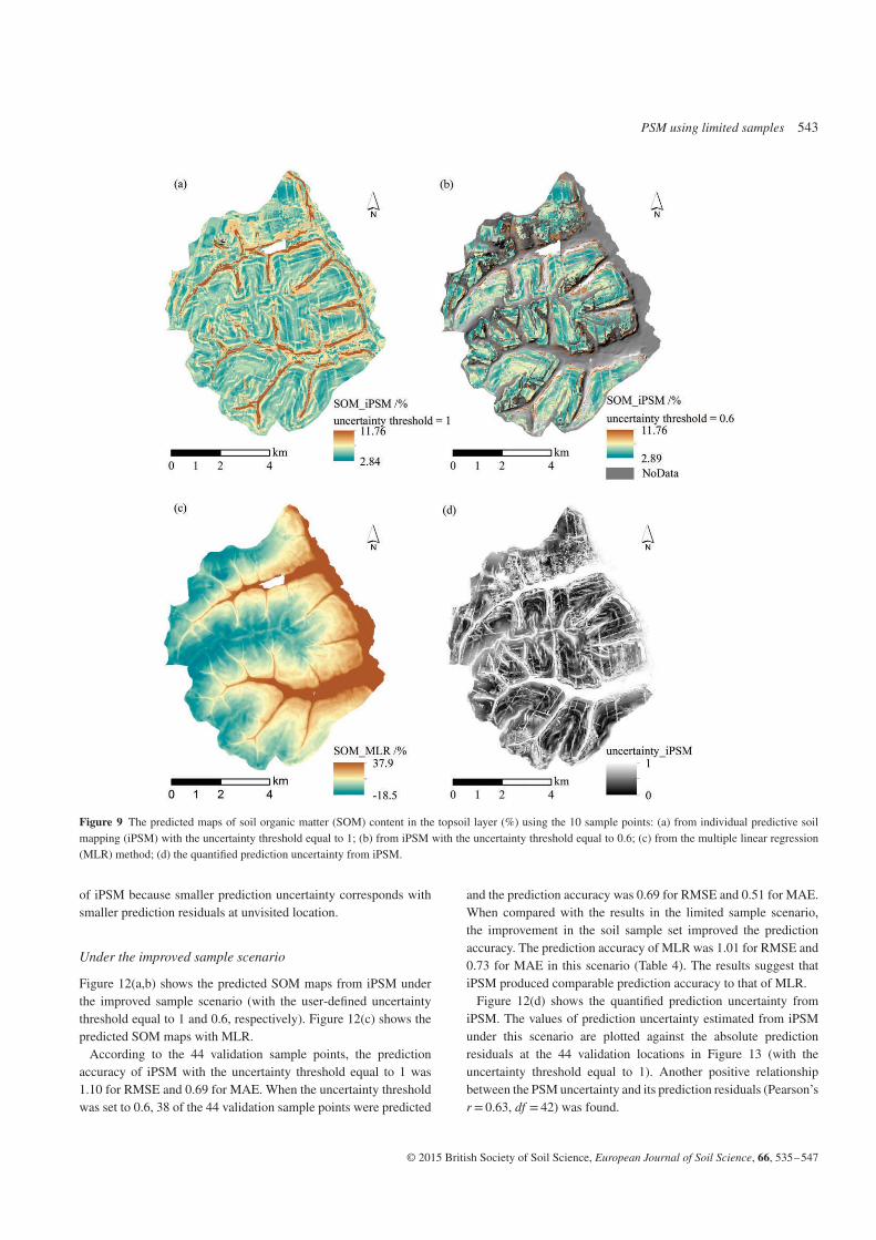
Under the limited sample scenario
Figure 9(a,b) shows the predicted SOM maps from iPSM under thelimited sample scenario with the user-defined uncertainty thresholdequal to 1 and 0.6, respectively. The spatial distribution of SOMcontent (%) in the topsoil layer (Figure 9a,b) matches our under-standing of how the terrain and vegetation environment influenceSOM content. Thus on upper-to-middle slopes erosive processestend to be the dominant processes that reduce the soil organicmatter content in the topsoil layer; on lower-to-toe slopes whichare often gentle depositional processes tend to be the dominantprocesses that usually lead to larger SOM contents in the top-soil layer. This pattern is obviously disturbed by vegetation con-ditions: the straight lines with large SOM content (%) correspondto field roads between farmland fields, where trees and grasses aregrowing.
Figure 9(c) shows the predicted SOM map from MLR underthe limited sample scenario. The SOM content (%) in the topsoilpredicted by MLR generally had a similar spatial distributionpattern to that from iPSM. The upper-to-middle steep slopes wereassociated with relatively small values while the lower-to-toe gentle
slopes were associated with relatively large values. However, somespatial details, such as the sharp changes across the field roads,are not present on the map. In addition, the predicted values ofSOM content from MLR ranged from −18.5 to 37.9%, which isbeyond the value range of the 10 soil samples. This is because ofthe limitation of the 10 soil samples, which are not representativeof the entire study area. The unrealistic extrapolation of the linearmodel at the location that cannot be represented by existing samplesleads to unrealistic prediction results.
The prediction accuracies of iPSM and MLR evaluated by the 44validation sample points are compared in Table 4. Those of iPSMwith an uncertainty threshold equal to 1 produced better predictionaccuracy (1.43 for RMSE and 1.16 for MAE) than those fromMLR (8.54 for RMSE and 7.34 for MAE). In addition, when theuncertainty threshold of iPSM was decreased to 0.6, 12 of the 44validation sample points were predicted and the prediction accuracyof iPSM was increased to 1.06 for RMSE and 0.91 for MAE. Thesmaller uncertainty threshold improved the prediction accuracy ofiPSM but left a greater area as ‘NoData’. The absolute predictionerror at each validation location from iPSM was also compared withthat from iPSM (Figure 10). At each individual validation location,iPSM produced better prediction accuracy.
Figure 9(d) shows the quantified prediction uncertainty fromiPSM under the limited sample scenario. Because the 10 soil
distance / m
sem
ivar
ianc
e
0.5
1.0
1.5
500 1000 1500 2000 2500 3000
0
0
Figure 8 The Gaussian semivariogram (nugget= 0, range= 1000,sill= 0.5) based on the residuals of the regression of soil organic matter(SOM) content in the topsoil layer (%) using the environmental covariatevalues at the 22 sample points.
samples were mainly located on side slopes (Figure 4) and representthose areas well, prediction uncertainty is generally small in thoseareas. In contrast, large prediction uncertainty values are assignedto ridges and valleys. In addition, because no sample points werelocated on the field roads, the prediction uncertainty for the roads isalso relatively large.
The values of prediction uncertainty estimated from iPSM areplotted against the absolute prediction residuals at the validationsample locations in Figure 11 (with uncertainty threshold= 1).Overall, there is a positive correlation between the PSM and itsprediction residuals (Pearson’s r = 0.54, df = 42). This indicatesthat the increases in the quantified prediction uncertainty arepositively correlated with the increases in prediction residualsproduced by iPSM. It further suggests that the quantified predictionuncertainty can be a good indicator of the prediction accuracy
Figure 9 The predicted maps of soil organic matter (SOM) content in the topsoil layer (%) using the 10 sample points: (a) from individual predictive soilmapping (iPSM) with the uncertainty threshold equal to 1; (b) from iPSM with the uncertainty threshold equal to 0.6; (c) from the multiple linear regression(MLR) method; (d) the quantified prediction uncertainty from iPSM.
of iPSM because smaller prediction uncertainty corresponds withsmaller prediction residuals at unvisited location.
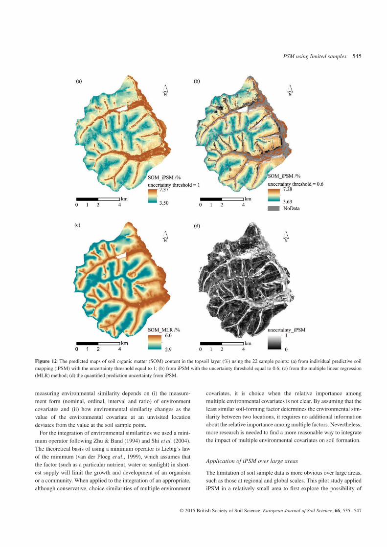
Under the improved sample scenario
Figure 12(a,b) shows the predicted SOM maps from iPSM underthe improved sample scenario (with the user-defined uncertaintythreshold equal to 1 and 0.6, respectively). Figure 12(c) shows thepredicted SOM maps with MLR.
According to the 44 validation sample points, the predictionaccuracy of iPSM with the uncertainty threshold equal to 1 was1.10 for RMSE and 0.69 for MAE. When the uncertainty thresholdwas set to 0.6, 38 of the 44 validation sample points were predicted
and the prediction accuracy was 0.69 for RMSE and 0.51 for MAE.When compared with the results in the limited sample scenario,the improvement in the soil sample set improved the predictionaccuracy. The prediction accuracy of MLR was 1.01 for RMSE and0.73 for MAE in this scenario (Table 4). The results suggest thatiPSM produced comparable prediction accuracy to that of MLR.
Figure 12(d) shows the quantified prediction uncertainty fromiPSM. The values of prediction uncertainty estimated from iPSMunder this scenario are plotted against the absolute predictionresiduals at the 44 validation locations in Figure 13 (with theuncertainty threshold equal to 1). Another positive relationshipbetween the PSM uncertainty and its prediction residuals (Pearson’sr = 0.63, df = 42) was found.
Table 4 The comparison of the prediction accuracies of individual predic-tive soil mapping (iPSM) and multiple linear regresssion (MLR) based onthe 44 validation sample points in the two scenarios
Figure 10 The comparison of prediction residuals from individual predic-tive soil mapping (iPSM) and multiple linear regression (MLR) at the 44validation sample points when the uncertainty threshold equals 0.6.
0
0.5
1
1.5
2
2.5
3
3.5
4
4.5
0 0.2 0.4 0.6 0.8 1
abso
lute
pre
dict
ion
resi
dual
prediction uncertainty
Pearson's r = 0.54 (df = 42)
Figure 11 The relationship between prediction uncertainty and absolutevalue of prediction residual produced by iPSM using the 10 soil samplepoints (with the uncertainty threshold equal to 1).
Discussion
Choosing an uncertainty threshold
The value of the uncertainty threshold controls the areas that canbe predicted with existing soil samples. The areas with a largeprediction uncertainty cannot be represented with existing soilsamples and the soil conditions over these areas are not predictedin iPSM according to a user-defined uncertainty threshold. This
strategy helps to avoid unrealistic extrapolation and makes iPSMuse the existing soil samples more appropriately.
As the uncertainty threshold takes smaller values, the area whereiPSM can make a prediction shrinks (Figures 9, 12). A small valueof uncertainty threshold leads to a strict criterion to determinewhether an unvisited location can be represented and thus can bepredicted from existing soil sample points. For example, under thelimited sample scenario with the uncertainty threshold set to 0.6(Figure 9b), only the locations where the environmental similaritiesto the existing soil samples were larger than 0.4 (1− 0.6) could bepredicted. Those locations were mainly on the side slopes, which arethe landforms well represented by the 10 soil samples. In contrast, alarge value of uncertainty threshold leads to a poor criterion, whichmeans that more areas can be represented and thus predicted by theexisting soil samples (Figure 9a).
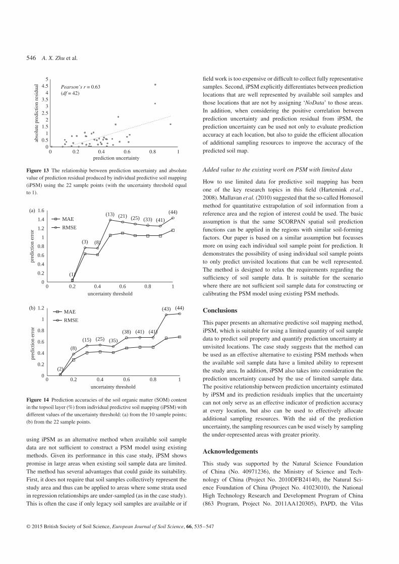
The value of the uncertainty threshold also influences the predic-tion accuracy. The overall accuracies of the predicted SOM mapsfrom iPSM by using different values of uncertainty thresholds wereevaluated by the 44 validation samples. Figure 14 shows that RMSEand MAE increased as the uncertainty threshold increased underthe two scenarios. The number next to each point is the number ofvalidation samples that were predicted when using the correspond-ing uncertainty threshold. The iPSM method thus has the advantageof controlling the quality of the prediction through its uncertaintythreshold; when choosing a value for the uncertainty threshold atrade-off needs to be made between prediction accuracy and theareas that can be predicted using the existing soil samples.
Selection of environmental covariates
When selecting the environmental covariates, the ultimate goal is todescribe the environmental conditions associated with the targetedsoil property as accurately as possible and all components of Jenny’sequation (Jenny, 1941) need to be considered. However, one alsoneeds to consider the effectiveness of environmental covariatesin indicating the spatial variation of soil, and the availability ofdata sources for calculation (Zhu et al., 2001). In our study onlythe environmental covariates describing topographic and vegetationconditions were used. One reason is that the study area wasrelatively small and climate conditions and parent materials aregenerally similar over the area; another reason is that it is relativelyeasy to obtain data characterizing terrain and vegetation conditions.With a more complex study area, more types of environmentalcovariates should be involved.
Measurement of environmental similarities
The measurement of environmental similarity is a crucial step iniPSM. Currently a Boolean operator is used for nominal and ordinalcovariates and a Gaussian-shaped function (Equation (3)) is usedfor interval and ratio covariates. Certainly other similarity/distancemeasurements defined in the environmental feature space, such astaxonomic distance (Minasny & McBratney, 2007), Gower simi-larity coefficient (Gower, 1971), Euclidian distance or Manhattandistance, can also be used. The choice of the method used for
Figure 12 The predicted maps of soil organic matter (SOM) content in the topsoil layer (%) using the 22 sample points: (a) from individual predictive soilmapping (iPSM) with the uncertainty threshold equal to 1; (b) from iPSM with the uncertainty threshold equal to 0.6; (c) from the multiple linear regression(MLR) method; (d) the quantified prediction uncertainty from iPSM.
measuring environmental similarity depends on (i) the measure-ment form (nominal, ordinal, interval and ratio) of environmentcovariates and (ii) how environmental similarity changes as thevalue of the environmental covariate at an unvisited locationdeviates from the value at the soil sample point.
For the integration of environmental similarities we used a mini-mum operator following Zhu & Band (1994) and Shi et al. (2004).The theoretical basis of using a minimum operator is Liebig’s lawof the minimum (van der Ploeg et al., 1999), which assumes thatthe factor (such as a particular nutrient, water or sunlight) in short-est supply will limit the growth and development of an organismor a community. When applied to the integration of an appropriate,although conservative, choice similarities of multiple environment
covariates, it is choice when the relative importance amongmultiple environmental covariates is not clear. By assuming that theleast similar soil-forming factor determines the environmental sim-ilarity between two locations, it requires no additional informationabout the relative importance among multiple factors. Nevertheless,more research is needed to find a more reasonable way to integratethe impact of multiple environmental covariates on soil formation.
Application of iPSM over large areas
The limitation of soil sample data is more obvious over large areas,such as those at regional and global scales. This pilot study appliediPSM in a relatively small area to first explore the possibility of
Figure 13 The relationship between prediction uncertainty and absolutevalue of prediction residual produced by individual predictive soil mapping(iPSM) using the 22 sample points (with the uncertainty threshold equalto 1).
(1)
(3) (8)
(13) (21) (25) (33) (41)(44)
0
0.2
0.4
0.6
0.8
1
1.2
1.4
1.6
0 0.2 0.4 0.6 0.8 1
pred
ictio
n er
ror
uncertainty threshold
MAERMSE
(a)
(2)
(8)(15) (25) (35)
(38) (41) (41)
(43) (44)
0
0.2
0.4
0.6
0.8
1
1.2
0 0.2 0.4 0.6 0.8 1
pred
ictio
n er
ror
uncertainty threshold
MAERMSE
(b)
Figure 14 Prediction accuracies of the soil organic matter (SOM) contentin the topsoil layer (%) from individual predictive soil mapping (iPSM) withdifferent values of the uncertainty threshold: (a) from the 10 sample points;(b) from the 22 sample points.
using iPSM as an alternative method when available soil sampledata are not sufficient to construct a PSM model using existingmethods. Given its performance in this case study, iPSM showspromise in large areas when existing soil sample data are limited.The method has several advantages that could guide its suitability.First, it does not require that soil samples collectively represent thestudy area and thus can be applied to areas where some strata usedin regression relationships are under-sampled (as in the case study).This is often the case if only legacy soil samples are available or if
field work is too expensive or difficult to collect fully representativesamples. Second, iPSM explicitly differentiates between predictionlocations that are well represented by available soil samples andthose locations that are not by assigning ‘NoData’ to those areas.In addition, when considering the positive correlation betweenprediction uncertainty and prediction residual from iPSM, theprediction uncertainty can be used not only to evaluate predictionaccuracy at each location, but also to guide the efficient allocationof additional sampling resources to improve the accuracy of thepredicted soil map.
Added value to the existing work on PSM with limited data
How to use limited data for predictive soil mapping has beenone of the key research topics in this field (Hartemink et al.,2008). Mallavan et al. (2010) suggested that the so-called Homosoilmethod for quantitative extrapolation of soil information from areference area and the region of interest could be used. The basicassumption is that the same SCORPAN spatial soil predictionfunctions can be applied in the regions with similar soil-formingfactors. Our paper is based on a similar assumption but focussesmore on using each individual soil sample point for prediction. Itdemonstrates the possibility of using individual soil sample pointsto only predict unvisited locations that can be well represented.The method is designed to relax the requirements regarding thesufficiency of soil sample data. It is suitable for the scenariowhere there are not sufficient soil sample data for constructing orcalibrating the PSM model using existing PSM methods.
Conclusions
This paper presents an alternative predictive soil mapping method,iPSM, which is suitable for using a limited quantity of soil sampledata to predict soil property and quantify prediction uncertainty atunvisited locations. The case study suggests that the method canbe used as an effective alternative to existing PSM methods whenthe available soil sample data have a limited ability to representthe study area. In addition, iPSM also takes into consideration theprediction uncertainty caused by the use of limited sample data.The positive relationship between prediction uncertainty estimatedby iPSM and its prediction residuals implies that the uncertaintycan not only serve as an effective indicator of prediction accuracyat every location, but also can be used to effectively allocateadditional sampling resources. With the aid of the predictionuncertainty, the sampling resources can be used wisely by samplingthe under-represented areas with greater priority.
Acknowledgements
This study was supported by the Natural Science Foundationof China (No. 40971236), the Ministry of Science and Tech-nology of China (Project No. 2010DFB24140), the Natural Sci-ence Foundation of China (Project No. 41023010), the NationalHigh Technology Research and Development Program of China(863 Program, Project No. 2011AA120305), PAPD, the Vilas
Associate Award, the Hammel Faculty Fellow Award, the ManasseChair Professorship from the University of Wisconsin-Madison,and the ‘One-Thousand Talents’ Program of China. Chengzhi Qin isgrateful for the support from the National Science and TechnologySupport Program (No. 2013BAC08B03-4). The authors would alsolike to express their appreciation of the valued comments from DrD.G. Rossiter from the International Institute for Geo-InformationScience and Earth Observation (ITC) of the University of Twente.
References
Beven, K.J. & Kirkby, N.J. 1979. A physically based variable contributingarea model of basin hydrology. Hydrological Sciences Bulletin, 24,43–69.
de Gruijter, J.J., Brus, D.J., Bierkens, M.F.P. & Knotters, M. 2006. Sampling
for Natural Resource Monitoring. Springer, New York.Florinsky, I.V. 2011. Digital Terrain Analysis in Soil Science and Geology.
Elsevier/Academic Press, Amsterdam.Gower, J.C. 1971. A general coefficient of similarity and some of its
M. 2008. Digital Soil Mapping with Limited Data. Springer Sci-ence+Business Media LLC, New York.
Hudson, B.D. 1992. The soil survey as a paradigm-based science. Soil
Science Society of America Journal, 56, 836–841.Jenny, H. 1941. Factors of Soil Formation: A System of Quantitative
Pedology. Dover Publication, New York.Johnson, C.J., Hurley, M., Rapaport, E. & Pullinger, M. 2012. Using
expert knowledge effectively: lessons from species distribution modelsfor wildlife conservation and management. In: Expert Knowledge and its
Application in Landscape Ecology (eds A.H. Perera, C.A. Drew & C.J.Johnson), pp. 153–171. Springer, New York.
Kienast-Brown, S. & Boettinger, J.L. 2007. Land cover classification fromLandsat imagery for mapping dynamic wet and saline soils. In: DigitalSoil Mapping: An Introductory Perspective. Developments in Soil Science
(eds P. Lagacherie, A.B. McBratney & M. Voltz), pp. 235–244. Elsevier,Amsterdam.
Liu, F., Geng, X.Y., Zhu, A.X., Fraser, W. & Arnie, W. 2012. Soil texturemapping over low relief areas using land surface feedback dynamicpatterns extracted from MODIS. Geoderma, 171-172, 44–52.
Mallavan, B.P., Minasny, B. & McBratney, A.B. 2010. Homosoil, amethodology for quantitative extrapolation of soil information across theglobe. In: Bridging Research, Environmental Application, and Operation(eds J.L. Boettinger, D.W. Howell, A.C. Moore, A.E. Hartemink & S.Kienast-Brown), pp. 137–149. Springer, Dordrecht.
McBratney, A.B., Mendonça-Santos, M.L. & Minasny, B. 2003. On digitalsoil mapping. Geoderma, 117, 3–52.
Mendonça-Santos, M.L., McBratney, A.B. & Minasny, B. 2006. Soilprediction with spatially decomposed environmental factors. In: Digital
SoilMapping: An Introductory Perspective. Developments in Soil Science
(eds P. Lagacherie, A.B. McBratney & M. Voltz), pp. 269–278. Elsevier,Amsterdam.
Minasny, B. & McBratney, A.B. 2006. A conditioned latin hypercubemethod for sampling in the presence of ancillary information. Computers& Geosciences, 32, 1378–1388.
Minasny, B. & McBratney, A.B. 2007. Incorporating taxonomic distanceinto spatial prediction and digital mapping of soil classes. Geoderma, 142,285–293.
Nield, S.J., Boettinger, J.L. & Ramsey, R.D. 2007. Digitally mapping gypsicand natric soil areas using Landsat ETM data. Soil Science Society ofAmerica Journal, 71, 245–252.
Qi, F. & Zhu, A.X. 2003. Knowledge discovery from soil maps usinginductive learning. International Journal of Geographical InformationScience, 17, 771–795.
Qin, C.Z., Zhu, A.X., Shi, X., Li, B.L., Pei, T. & Zhou, C.H. 2009. Thequantification of spatial gradation of slope positions. Geomorphology,110, 152–161.
Qin, C.Z., Zhu, A.X., Pei, T., Li, B.L., Scholten, T., Behrens, T. et al. 2012.An approach to computing topographic wetness index based on maximumdownslope gradient. Precision Agriculture, 12, 32–43.
Ramsey, C.A. & Hewitt, A.D. 2005. A methodology for assessing samplerepresentativeness. Environmental Forensics, 6, 71–75.
Scull, P., Franklin, J., Chadwick, O.A. & McArthur, D. 2003. Predictive soilmapping: a review. Progress in Physical Geography, 27, 171–197.
Shi, X., Zhu, A.X., Burt, J., Qi, F. & Simonson, D. 2004. A case-basedreasoning approach to fuzzy soil mapping. Soil Science Society ofAmerica Journal, 68, 885–894.
Stevens, S.S. 1946. On the theory of scales of measurement. Science, 103,677–680.
van Groenigen, J.W. & Stein, A. 1998. Constrained optimization of spatialsampling using continuous simulated annealing. Journal of Environmen-tal Quality, 27, 1078–1086.
van der Ploeg, R.R., Bohm, W. & Kirkham, M.B. 1999. On the origin ofthe theory of mineral nutrition of plants and the law of the minimum. SoilScience Society of America Journal, 63, 1055–1062.
Webster, R. & Oliver, M.A. 1990. Statistical Methods in Soil and LandResource Survey. Oxford University Press, Oxford.
Yang, L., Zhu, A.X., Li, B.L., Qin, C.Z., Pei, T., Liu, B.Y. et al. 2007.Extraction of knowledge about soil-environment relationship for soilmapping using fuzzy c-means (FCM). Acta Pedologica Sinica, 44,784–791 (in Chinese).
Zhu, A.X. 1999. A personal constructed-based knowledge acquisitionprocess for natural resource mapping using GIS. International Journalof Geographic Information Systems, 13, 119–141.
Zhu, A.X. 2001. Modeling spatial variation of classification uncertaintyunder fuzzy logic. In: Spatial Uncertainty in Ecology (eds C. Hun-saker, M.F. Goodchild, M. Friedl & T. Case), pp. 330–350. Springer,New York.
Zhu, A.X. & Band, L.E. 1994. A knowledge-based approach to dataintegration for soil mapping. Canadian Journal of Remote Sensing, 20,408–418.
Zhu, A.X., Band, L.E., Vertessy, R. & Dutton, B. 1997. Derivation of soilproperties using a soil land inference model (SoLIM). Soil Science Societyof America Journal, 61, 523–533.
Zhu, A.X., Hudson, B., Burt, J.E. & Lubich, K. 2001. Soil mapping usingGIS, expert knowledge, and fuzzy logic. Soil Science Society of AmericaJournal, 65, 1463–1472.
Zhu, A.X., Yang, L., Li, B., Qin, C., English, E., Burt, J.E. et al.2008. Purposefully sampling for digital soil mapping. In: Dig-ital Soil Mapping with Limited Data (eds A.E. Hartemink, A.B.McBratney & M.L. Mendonca Santos), pp. 233–245. Springer-Verlag,New York.
Zhu, A.X., Liu, F., Li, B.L., Pei, T., Qin, C.Z., Liu, G.H. et al. 2010.Differentiation of soil conditions over flat areas using land surfacefeedback dynamic patterns extracted from MODIS. Soil Science Societyof America Journal, 74, 861–869.