Predictive Tree: An Efficient Index for Predictive

Queries On Road Networks

Abdeltawab M. Hendawi1,2 Jie Bao1 Mohamed F. Mokbel1 Mohamed Ali2,3

1Department of Computer Science and Engineering, University of Minnesota, Minneapolis, MN, USA1{hendawi, baojie, mokbel}@cs.umn.edu

2Institute of Technology, University of Washington, Tacoma, WA, USA2{hendawi, mhali}@uw.edu3Microsoft Corporation

3mali@microsoft.com

Abstract—Predictive queries on moving objects offer an im-portant category of location-aware services based on the objects’expected future locations. A wide range of applications utilize thistype of services, e.g., traffic management systems, location-basedadvertising, and ride sharing systems. This paper proposes anovel index structure, named Predictive tree (P-tree), for process-ing predictive queries against moving objects on road networks.The predictive tree: (1) provides a generic infrastructure foranswering the common types of predictive queries includingpredictive point, range, KNN, and aggregate queries, (2) updatesthe probabilistic prediction of the object’s future locationsdynamically and incrementally as the object moves around onthe road network, and (3) provides an extensible mechanism tocustomize the probability assignments of the object’s expectedfuture locations, with the help of user defined functions. Theproposed index enables the evaluation of predictive queries inthe absence of the objects’ historical trajectories. Based solely onthe connectivity of the road network graph and assuming thatthe object follows the shortest route to destination, the predictivetree determines the reachable nodes of a moving object withina specified time window T in the future. The predictive treeprunes the space around each moving object in order to reducecomputation, and increase system efficiency. Tunable thresholdparameters control the behavior of the predictive trees by tradingthe maximum prediction time and the details of the reportedresults on one side for the computation and memory overheadson the other side. The predictive tree is integrated in the contextof the iRoad system in two different query processing modes,namely, the precomputed query result mode, and the on-demandquery result mode. Extensive experimental results based on largescale real and synthetic datasets confirm that the predictive treeachieves better accuracy compared to the existing related work,and scales up to support a large number of moving objects andheavy predictive query workloads.

I. INTRODUCTION

The availability of hundreds of millions of smart phones [6]

in users’ hands during their movements in daily lives fired the

explosion of a vast number of location aware services [5],

[11], [20], [29]. Predictive queries [10], [12], [13] offer a

fundamental type of location-based services based on users’

future locations. Common types of predictive spatial queries

include predictive range query, e.g., “find all hotels that are

This work is partially supported by the National Science Foundation, USA,under Grants IIS-0952977 and IIS-1218168.

located within two miles from a user’s anticipated location

after 30 minutes“, predictive KNN query, e.g., “find the three

taxis that are closest to a user’s location within the next

10 minutes“, and predictive aggregate query, e.g., “find the

number of cars expected to be around the stadium during the

next 20 minutes“.

In fact, Predictive queries are beneficial in various types

of real applications such as (1) traffic management, to predict

areas with high traffic in the next half hour, so appropriate

decisions are taken before congestion appears, (2) location-

aware advertising, to distribute coupons and sales promotions

to customers more likely to show up around a certain store

during the sale time in the next hour, (3) routing services,

to take into consideration the predicted traffic on each road

segment to find the shortest path of a user’s trip starting after

15 minutes from the present time, (4) ride sharing systems, to

match the drivers that will pass by a rider’s location within

few minutes, and (5) store finders, to recommend the closest

restaurants to a user’s predicted destination in 15 minutes.

In this paper, we address the problem of how to process pre-

dictive queries for moving objects on road networks efficiently.

To this end, we introduce a novel index structure, named the

Predictive tree (P-tree), proposed to precompute the predicted

moving objects around each node in the underlying road

network graph over time. The predictive tree is best described

as generic and extensible, from a functionality perspective,

dynamic and tunable from a performance perspective.

A. Challenges

Existing studies on predictive query processing have gone

a long way in advancing predictive location-based services.

However, existing techniques suffer from both functional

limitations and performance deficiencies. From a functional

perspective, they suffer from one or more of the following

limitations: (1) They consider an Euclidean space [9], [28],

[25], [30] where objects can move freely in a two dimensional

space. Yet, practical predictive location-based services target

moving objects on road networks as described by the motivat-

ing applications earlier in this section. (2) Many techniques

utilize prediction models that must be trained using a massive

a mount of objects’ historical trajectories in order to produce

accurate predictions [2], [9], [13], [15], [24], [28]. However,

practical scenarios and industrial experience reveal that such

historical data is not easily obtainable for many reasons, either

due to users’ privacy and data confidentiality on one side or

due to the unavailability of historical data in rural areas on the

other side. (3) Most of the previous solutions were designed to

support a specific query type only, e.g., [13], [25], [30] support

predictive range query, [3], [22], [30] support predictive KNN

query, and [9], [24] support predictive aggregate query.

B. Approach

Before summarizing the contributions of the proposed pre-

dictive tree index, we briefly highlight the basic idea of the

index in order to build the proper context. Once an object

starts a trip, we construct a predictive tree for this object

such that the object’s start node in the road network graph

becomes the root of the tree. The predictive tree consists

of the nodes reachable within a certain time frame T from

the object’s start location. More specifically, we assume that

moving objects follow shortest paths during their travel from

source to destination [16], [18]. Hence, we organize the nodes

inside the predictive tree according to the shortest path from

the object’s start node, which is marked as the root of the tree.

Accordingly, each branch from the root node to any node in

the tree represents the shortest route from the root to this node.

Then, our prediction is based on a probability assignment

model that assigns a probability value to each node inside the

object’s predictive tree. In general, the probability assignment

is made according to the node’s position in the tree, the travel

time between the object and this node and the number of the

sibling nodes. In practice, the probability assignment process

is tricky and varies from one application to another.

At each node in the given road network that is indexed in

R-tree, we keep track of a list of objects predicted to appear

in this node, along with their probabilities, and travel time

cost from the objects’ current locations to this node. This list

represents a raw precomputed answer that can be customized

according to the type of the received query (i.e., point, range

or kNN predictive query) at query processing time. When an

object moves from its current node to a different node, we

incrementally update the predictive tree by pruning all nodes

in the tree that are no longer accessible through a shortest route

from the object’s new location. Mostly, this pruning shrinks

the number of possible destinations, yet, increases the focus of

the prediction. Consequently, the precomputed answer at each

node in the object predictive tree is updated to accommodate

the effect of the object’s movements. This update is reflected

to the original nodes in the road network. When a predictive

query is received, we fetch the up-to-date answer from the

node of interest and compile it according to the query type.

To adjust the behavior of the predictive tree and, hence,

control the overall predictive query processing performance,

we leverage two tunable parameters, a maximum time Tand a probability threshold P . These parameters compromise

between the maximum prediction time a predictive tree can

support and the details in the reported query results on one

side, and system resources overheads, i.e., CPU and memory,

on the other side.

The proposed predictive tree is implemented within the

iRoad framework. The iRoad offers two query processing

modes of leveraging the predictive tree to control the inter-

action between its components: (1) the precomputed query

result mode, in which the predicted results are computed and

materialized in advance; and (2) the on-demand query result

mode which is a lazy approach that postpones all computation

till a query is received.

C. Contributions

In general, the contributions of this paper can be summa-

rized as follows:

• We propose a novel data structure named Predictive tree

(P-tree) that supports predictive queries against moving

objects on road networks.• We introduce a probability model that computes the like-

lihood of a node in the road network being a destination

to a moving object. The probability model is introduced

to the predictive tree as a user defined function and is

handled as a black box by the index construction and

maintenance algorithms.• We introduce two tunable parameters T and P that are

experimentally proved to be efficient tools to control

the predictive tree index, the system performance, the

prediction time, and the results details as well.• We provide an incremental approach to update the pre-

dictive tree as objects move around. Hence, we utilize

the existing index structure and incur minimal cost in

response to the movement of the object.• We propose the iRoad framework that leverages the

introduced predictive tree to support a wide variety of

predictive queries including predictive point, range, and

KNN queries.• we provide an experimental evidence based on real and

synthetic data that our introduced index structure is

efficient in terms of query processing, scalable in terms

of supporting large number of moving objects and heavy

query workloads, and achieves a high-quality prediction

without the need to reveal objects’ historical data.

The remainder of this paper is organized as follows. Sec-

tion II sets the preliminaries and defines our problem. Sec-

tion III presents the iRoad system. Section IV describes the

the predictive tree and its associated construction, maintenance

and querying algorithms. Experimental results are presented in

Section V. The study of related work is given in Section VI.

Finally, Section VII concludes the paper.

II. PRELIMINARIES

In this section, we formalize the basic predictive query

we address in this paper. Then, we define different types of

predictive queries that the predictive tree can support within

the iRoad framework. After that, we explain the intuition of

the leveraged prediction model.

Fig. 1. iRoad System Architecture

A. Basic Query

In this paper, we focus on addressing the predictive point

query as our basic query on the road network. In this query, we

want to find out the moving objects with their corresponding

probabilities that are expected to be around a specified query

node in the road network within a future time period. The

example of such query could be like, “Find out all the

cars that may pass by my location in the next 10 mins”.

The predictive point query we address in this paper can be

formalized as: “Given (1) a set of moving objects O, (2) a

road network graph G(N, E, W), where N is the set of nodes,

E is the set of edges, and W is the edge weights, i.e., travel

times, and (3) a predictive point query Q(n, t), where n ∈ N,

and t is a future time period, we aim to find the set of objects R

∈ O expected to show up around the node n within the future

time t. The returned result should identify the objects along

with their probabilities to show up at the node of interest. For

example, within the next 30 mins, object o1 is expected to be

at node n3 with probability 0.8, R(Q(n3,30)) = {< o1,0.8>}.

B. Extensions

We consider the aforementioned predictive point query as a

building block upon which our framework can be extended

to support other types of predictive queries including: (i)

Predictive range query, where a user defines a query region

that might contain more than one node and asks for the list

of objects expected to be inside the boundaries of that region

within a specified future time, (ii) Predictive KNN query to

find out the most likely K objects expected to be around

the node of interest within a certain time period, and (iii)

Predictive aggregate query to return the number of objects

predicted to be within a given location in the next specified

time duration.

C. Prediction Model

Our prediction model employed by the introduced predictive

tree index structure is based on two corner stones. (1) The

assumption that objects follow the shortest paths in their

routing trips. The intuition behind this assumption is based

on the fact that in most cases, the moving objects on road

networks, e.g., vehicles, travel through shortest routes to their

destinations [16], [18]. In fact, this assumption is aligned with

the observation in [4] that moving objects do not use random

paths when traveling through the road network, rather they

follow optimized ones, e.g., fastest route. As a result, this

(a) Network & Objects

(b) Predictive Trees Integrated With R-Tree

Fig. 2. Example Of The Proposed Index Structure

model prevents the looping case that appears in the traditional

turn-by-turn probability model and assigns a probability value

for the moving object to turn when facing an intersection [13].

(2)The probability assignment model that assigns a proba-

bility value to each node inside the object’s predictive tree.

In fact, the probability assignment is affected by the node’s

position with respect to the root of the tree, the travel time

cost between the object in its current location to this node,

and the number of the sibling nodes. In general, our predictive

tree is designed to work with different probability assignment

models. For example, a possible probability model can give

higher values to nodes in business areas, e.g., down town,

rather than those in the suburbs. In our default probability

model, each node in the predictive tree has a value equal to

one divided by the number of nodes accessible from the root

within a certain time range.

III. THE IROAD SYSTEM

The proposed predictive tree is implemented in the context

of the iRoad System. More precisely, the predictive tree and its

construction, maintenance and querying algorithms form the

core of the iRoad System. The iRoad System is a scalable

framework for predictive query processing and analysis on

road networks. The architecture of the iRoad system consists

of three main modules, namely, the state manager, the pre-

dictive tree builder and the query processor, Figure 1. In this

section, we present an overview of the iRoad System and give

a brief description of its key components. Moreover, we focus

on the interaction and workflow between these components

under both the precomputed query result mode and the on-

demand query result mode.

A. State Manager

The state manager is a user facing module that receives

a stream of location updates from the moving objects being

monitored by the system. The state manager maintains the

following data structures. (1) An R-tree [7] that is generated

on the underlying road network graph. It differs from the

conventional R-tree in that at each leaf node, i.e., a node

in the road network, in addition to storing the corresponding

MBR, it also keeps track of two lists: (a) current objects that

records the pointers to the objects around this node, and (b)

predicted objects that maintains the predicted results of the

objects that most likely to show up around that node. (2) A

trajectory buffer that stores the most recent one or more nodes

in the road network that are visited by the moving object

in its ongoing trip. (3) A predictive tree such that root of

a predictive tree is the current location of the moving object.

Figure 2(a) gives an example of a set of objects moving on

a road network, while Figure 2(b) depicts how the predictive

trees are integrated within the basic data structures layout to

facilitate the processing of predictive queries.

As we mentioned, the system can be running under either

(1) a precomputed query result mode or (2) an on-demand

query result mode. The first is the default mode inside the

iRoad framework. In either modes, upon the receipt of a

location update of a moving object, the R-tree is consulted and

the new location is mapped to its closest node Nnew in the

road network. If the new node Nnew is the same as the object’s

old node Nold, the object movement is not significant enough

to change the system’s state and no further action is taken.

Otherwise, the object has moved to a different node and an

evaluation of the impact of the object’s movement is triggered

in the system. We differentiate between the precomputed and

the on-demand query result modes as follows.

Precomputed query result mode: In this mode, the predic-

tive tree builder is invoked immediately once the moving ob-

ject changes its current node and, consequently, the predictive

tree is either constructed from scratch or updated in response

to the object’s movement. Remember that the predictive tree

is constructed from scratch if the incoming location update

belongs to a new object that is being examined by the system

for the first time. Also, the predictive tree is constructed from

scratch if Nnew is not a child of the root of the object’s in-

hand predictive tree. As will be described in Section IV, this

case happens if the object decided not to follow the shortest

path, e.g., made a u-turn or started a new trip. Otherwise,

the tree is incrementally maintained. Note that, in this mode,

the trajectory buffer data structure boils down to one single

node (i.e., the current node) of the moving object because of

the eagerness to update the predictive tree with the receipt of

every location update. Hence, the past trajectory is entirely

factored in the predictive tree.

On-demand query result mode: In this mode, the tra-

jectory buffer stores all nodes the moving object passed by

since the start of its current trip. Initially, We do not perform

any computation until a query is received. Then, we identify

the vicinity nodes within the time range determined by the

query. Those nodes might contribute in the predicted results.

For each object in these nodes, we construct its predictive tree

and run a series of updates according to the list of passed

nodes in its trajectory buffer, Figure 3. For example, in this

figure, nodes A, G, and E are within the time range specified

in the query at node B. Then, we construct the predictive tree

for each object, O1, O2, O3, in those nodes and update them

according the passed nodes by each one. Obviously, O1, O3

will contribute in the predicted objects at node B, while O2

will not contribute as node B is no longer a possible destination

Fig. 3. On-Demand Approach

for O2 based on its trajectory buffer. Then, we get rid of any

data structure, i.e., the predictive trees and predicted results,

directly once the query processing is completed and the results

are carried back to the query issuer. We ending by adding the

object’s current node Nnew, i.e,. Node B in this example, to

the object’s trajectory buffer.

B. Predictive Tree Builder

The predictive tree builder is the component that encom-

passes the predictive tree construction and maintenance algo-

rithms. It takes as input, (1) the moving object’s trajectory

buffer, (2) the moving object’s current predictive tree (if

exists), (3) the tunable parameters (T and P) that trade the

prediction length and accuracy for system’s resources, and (4)

a user defined probability assigned function. The predictive

tree builder reflects the most recent movements of the object

(as recorded in the object’s trajectory buffer) to the object’s

predictive tree. Upon the completion of a successful invocation

of the tree builder, an up-to-date predictive tree rooted at the

object’s current location is obtained and the object’s trajectory

buffer is modified to accommodate the object’s current node.

The predictive tree builder is invoked in two different ways.

In a precomputed query result mode, the builder is invoked by

the state manager upon the receipt of every location update.

The state manager pushes the incoming location update of a

moving object Oi to the predictive tree builder that eagerly

reflects the location update in the predictive tree of Oi.

Afterwards, the tree builder updates the precomputed query

results at every node in the road network that is on the shortest

path route from the object Oi’s current location.

In an on-demand query result mode, the predictive tree

builder is invoked by the query processor once a query Q

is received. The predictive tree builder consults the road

network graph and retrieves a list of nodes Nvicinity that are

within the time distance determined by the query Q. Then,

it pulls, from the state manager, the predictive trees and the

trajectory buffers of moving objects whose current nodes are

in Nvicinity . In other words, lazy or selective processing of

moving objects that are believed to affect the query result

is carried over without taking the burden of updating the

predictive tree of every single moving object in the system.

C. Query processor

The main goal behind predictive query processing in the

iRoad system is to be generic and to provide an infrastructure

for various query types. This goal is achieved by mapping a

query type to a set of nodes (Nvicinity) in the road network

graph such that the query result is satisfied by predictions

Algorithm 1 Predictive Tree Construction

Input: Node n, T ime Range T , Road Network GraphG(N,E,W )

1: Step 1. Initialize the data structures2: Set n as the root of the Predictive Tree PT3: Visited nodes list NL ← ∅4: Min-Heap MH ← ∅5: for all Edge ei connected with n do6: Insert the node ni ∈ ei → MH7: end for

8: Step 2. Expand the road network and create the predictive tree9: while the minimum time range Tmin in MH < T do

10: Get the node nmin with Tmin from MH11: if The nmin /∈ NL then

12: Insert nmin → PT13: Insert nmin → NL14: for all Edge ej connected with nmin do

15: Insert the node nj → MH16: end for17: end if

18: end while

19: Return PT

associated with these nodes. For predictive point queries as an

example, the point query is answered using the information

associated with the road network node that is closest to the

query point. For predictive range queries, all nodes in the range

are considered to compute the query result. For predictive

KNN queries, we sort those predicted objects associated with

Nvicinity based on their probabilities. Nvicinity is rationally

expanded till K objects are retrieved, if visible.

In a precomputed query result mode, generic results are

prepared in advance and are held in memory. The process is

triggered by an update in object’s location and the precom-

puted results are constructed/updated for all nodes along the

shortest path route of that object. Therefore, most of the work

is done during the location update time. Upon the receipt of

a query, the query processor fetches the precomputed results

only from nodes in Nvicinity , adapts them according to the

type of the received query and gives a low latency response

back to the user.

In an on-demand query result mode, nothing is precomputed

in advance and all computation will be performed after the

receipt of the user’s query. Nvicinity is identified and the pre-

dictive tree of objects whose current node belong to Nvicinity

are constructed/upadted as described earlier in this section.

Then, the results are collected and adapted to the query type

in a similar way to the precomputed result approach.

IV. PREDICTIVE TREE

In this section, we describe the proposed predictive tree

index structure that is leveraged inside the iRoad framework to

process predictive queries based on the predicted destinations

of the moving objects within a time period T . We first

introduce the main idea and the motivation to build the

predictive tree. After that, we provide a detailed description

for the two main operations in the predictive tree: 1) predictive

tree construction, and 2) predictive tree maintenance.

The idea of the predictive tree is to identify all the possible

destinations that a moving object could visit in a time period T

by traveling through the shortest paths. As there may only exist

one shortest path from a start node to a destination node, we

can guarantee it will be a tree structure (i.e., without any loop).

The intuition for constructing the predictive tree with a time

boundary T is based on two real facts: 1) most of the moving

objects travel through shortest path to their destinations [16],

[18], and 2) majority of the real life trips are within a time

period, e.g., 19 minutes [17], [18]. As a result, we only need

to care about the possible destinations reachable through a

shortest route from the object’s start location within a bounded

time period. Based on that, we build the predictive tree to hold

only the accessible nodes around a moving object and assign

a probability for each one of them.

The predictive trees leveraged in the iRoad system signif-

icantly improves the predictive query processing efficiency

for two main reasons. 1) The possible destinations of the

prediction shrinks as a result of using the time boundary T .

Yet, prediction computation is performed on few number of

nodes instead of millions of nodes in the underlying road

network, e.g., road network of California state in USA has

about 1,965,206 nodes and 5,533,214 edges [23]. 2) Inside the

predictive tree, we maintain only those nodes with probability

higher than a certain probability threshold parameter P , e.g.,

10%. By doing this, we cut down the computation overhead

consumed for continuously maintaining the predicted results at

each node in the predictive trees. Moreover, we control iRoad

to focus on those nodes that more likely to be reached by a

moving object. Yet, the query reported results can be more

reasonable to users.

A. Predictive Tree Construction

Main idea. When a moving object starts its trip on the

road network, we build a predictive tree based on its starting

location to predict its possible destinations within a certain

time frame T . We propose a best-first network expansion

algorithm for constructing predictive tree for time period T ,

e.g., 30 minutes. We set the object’s initial node as the

start node, then, we visit the nodes and edges on the road

network that are reachable using a shortest path from this start

node [21]. The algorithm proceeds to traverse and process the

edges in the road network based on the travel time cost from

the start node until all the costs to the remaining edges are

over T .

Algorithm. The pseudo code for the predictive tree con-

struction algorithm is given in Figure 1. The algorithm takes

the road network G = {N,E,W}, a starting node n and a

time range T as input. The algorithm consists of two main

steps:

• Initialization. We first initialize the predictive tree under

construction by setting the start node n as the root of the

tree. We also create the visited nodes list NL to store

the nodes that have been processed by the algorithm so

far. An empty min-heap, MH , is employed to order the

nodes based on its distance to the root node n. After that,

we insert the nodes that are directly connected with the

Fig. 4. Example of Constructing And Expanding The Predictive Tree Started At Node A.

root node n into the min-heap MH , (Lines from 2 to 7

in Algorithm 1).

• Expansion. We continuously pop the node nmin that is

the closest to the root node from the min-heap. Then,

we check if that node has been visited by our algorithm

before, which means there was a shorter path from the

root to this node nmin. If visited nodes list NL does not

contain nmin, we insert the node nmin to it as well as

a child to the current expanding branch of the predictive

tree PT . After that, we insert to the min-heap MH the

node nj that is connected with the yet processed node

nmin for further expansion. The algorithm stops when

the distance between the next closest node in the min-

heap is over the boundary T , (Lines from 8 to 18 in

Algorithm 1).

Example. Figure 4 gives an example for constructing a

predictive tree for node A from the given road network.

For this example, we set the time period T to 20 minutes.

Figure 4(a) gives the original road network structure, where

circles represent nodes and lines between nodes represent

edges and the number on each edge represents the time cost

to traverse that edge. In the first iteration, we start by setting

the root of the tree to node A. Then, we insert nodes B and

C into the min-heap, as they are the connected ones to the

root node A, Figure 4(b). After that, we expand the closest

child to the root, B, where we insert D and E into the min-

heap MH and put B in the predictive tree and the visited

nodes list NL as well, Figure 4(c). In the second iteration,

node C is the closest node to the root with travel time cost

equals 10 minutes. Yet, we insert C into the predictive tree in

addition to the visited nodes list. At the meanwhile, we put

B and F into the min-heap. In this turn, the cost from root

A to node B is 15 minutes, Figure 4(c). The next iteration

picks up the node B again from the min-heap MH . The

algorithm skips the processing for B, as it is already in the

visited node list NL. Accordingly, we continue the expansion

of node D, and insert E to the min-heap. After that, all the

remaining nodes in the min-heap have the distance more than

the time interval T . The algorithm terminates and returns the

constructed predictive tree, Figure 4(e).

Predictive Tree Expansion. As we mentioned above, the

iRoad framework can answer predictive queries up to a maxi-

mum time boundary T in the future. This means, the in-hand

predictive tree can not support prediction for object’s trips

that last longer than the specified future time T . Therefore,

to support those longer trips, we have to expand the tree to

make sure that its depth under the object new location is not

less than T . In this section, we explain how to expand the

predictive tree according to an object’s movements.

Main idea. The main idea to expand a predictive tree is to

locate the original predictive tree based on the start location of

the object. After that, we take the new location of the object

and make it as the new root for the just updated predictive tree.

Then, the new destinations of the moving objects are the nodes

located within the sub-tree underneath the new root. At the

meanwhile, all the other nodes will be discarded for the further

predication and processing. One important thing we have to

take into consideration while we are inserting new nodes to

the expanded predictive tree is that, all inserted nodes have

to be reached in a shortest path from the object’s start node.

This means, we can postpone the deletion of the data structures

used to build the original predictive tree until its corresponding

object finishes its trip. This decision is to avoid reconstructing

the predictive tree from scratch, instead, the expansion process

acts as one more iteration in the construction algorithm.

Example. Figure 4(f) gives an example for updating a

predictive tree according to the object movement. Figure 4(e)

gives the original predictive tree for the object o when it starts

the trip at node A. In this example, the object moves from the

starting location A to C. We get the current location of the

object and locate it to the new node C in the original predictive

tree. After that, the system returns C directly to the moving

object as the root for its expanded predictive tree. Then, only

the children of the new root, i.e., node F , will be considered

in the further processing.

B. Predictive Tree Maintenance

In this section, we explain how to maintain the constructed

predictive tree such that objects movements are reflected on

the structure of the tree as well as the probabilities of its nodes.

Main idea. When a moving object starts a new trip, we

get its start location and map it to the closest node in the

road network graph. Then, we dispatch the tree construction

module to construct a predictive tree with the root pointing

to the object’s start node. At this point, the tree construction

computes the probability of each node in the in-hand predictive

tree to be a destination to that object. If a node has a

probability higher than the predefined threshold parameter P ,

we insert the object to the list of predicted objects stored at

this node. When the object travels to its next node in the tree,

the predictive tree maintenance maintains the predicted results

Algorithm 2 Predictive Tree Maintenance

Input: Probability Threshold P , Time Range T , Current Node n, trajectory

buffer

1: if n = last added node in trajectory buffer then

2: return;3: else if (n is the first movement of o or movement to n violates shortest

path then

4: trajectory buffer ← ∅5: Construct the predictive tree PT for o rooted at n6: else if Tree depth underneath n < T then

7: Expand the predictive tree PT8: Prune the predictive tree PT9: Delete o from the list of predicted objects at ni

10: else

11: Prune the predictive tree PT12: Delete o from the list of predicted objects at ni

13: end if

14: for each node ni in PT do

15: Compute the probability P(ni)16: if P(ni)≥ P then

17: Insert o → list of predicted objects at ni

18: end if

19: end for20: Insert n → trajectory buffer

at each node in the tree as follows. (1) The predictive tree is

updated by changing its root to point out to the object current

node, and/or by extending the tree if its depth underneath the

objects’ current node is less than the time period T . (2) All

nodes other than those in the current subtree underneath the

new root will be pruned. Hence, we remove all occurrences

of that object along with its probability from the predicted

results at those pruned nodes. (3) The list of predicted objects

at the current subtree will be updated by either adding the

object to it, or modifying its probability in case the object

is already there. In fact, the predictive tree maintenance is a

core operation inside the predictive tree index structure, as it

is responsible for maintaining the tree and hence updating the

predicted objects at each node in the tree and reflecting that

to the nodes in the original road network graph.

Algorithm. Algorithm 2 gives the pseudo code for the

predictive tree maintenance algorithm. The algorithm takes

the trajectory buffer for the moving object o, and its current

node n, in addition to two system parameters, the probability

threshold P and time range for maximum predictable period

in the future T . Initially, we check if the object is still around

its original node, then, the algorithm does nothing, (Line 2 in

Algorithm 2). Otherwise, the algorithm preforms one or more

of the following possible steps.

(1) Construct New Predictive Tree. The algorithm examines

if the object starts a new trip by checking for two cases; (a) it

has not passed by any previous node, or (b) its recent move-

ment violates shortest path routing which internally means the

object moves to a node that is not a child of its previous node

within its predictive tree. For any of these cases, the algorithm

constructs a new predictive tree PT for the object o with a

root points to the object’s current node n, ( Lines 4, and 5, in

Algorithm 2).

(2) Maintain Existing Predictive Tree. If the object o takes

one more step toward its destination through a node in its

original predictive tree PT , we need to make sure that the

depth of the subtree underneath its current node n is greater

than or equal to the maximum prediction time T . If this is the

case, we prune the in-hand tree by cutting off all nodes not in

the subtree underneath the new root n, Line 11 in Algorithm 2.

Pruned nodes are no longer possible destinations to the object

o as they can not be reached in a shortest path from the object’s

current location. If it is not the case, the algorithm dispatches

the predictive tree expansion submodule, explained earlier in

this section, to extend the original tree PT such that the time

distance from the current node n to the end of PT is at least

equal to T . Then we prune the updated tree, (Lines 7, and 8

in Algorithm 2).

(3) Assign The Probability. After having the modified pre-

dictive tree PT for the object o, we compute the probability for

each node ni in PT being a possible destination to o, Line 15

in Algorithm 2. This is done according to the probability

assignment model, Section II-C.

(4) Maintain The Predicted Results. The aim of this step

is to make sure that the list of predicted objects stored with

each node in the road network get updated according to the

effect of the object’s movements. This is done by performing

the following two actions. (First) Within the pruning process

we have to delete any occurrence for the object o from the list

of predicted objects at the excluded nodes, (Lines 9, and 12

in Algorithm 2). (Second) After computing the probability of

each node in the current PT , we check if this probability

is above the given probability threshold P , we insert a new

record to the list of predicted results at the node ni, in case that

o is not in this list. Otherwise, we just modify its corresponding

probability value. This record consists of identifier for the

object o, its probability P(ni) to show up at ni, the travel

time from the tree root to the node ni,(Lines from 15 to 18 in

Algorithm 2). This list of predicted results will be used later by

the query processor module to evaluate users’ queries. Finally,

the algorithm updates the trajectory buffer to accommodate the

current node n, Line 20 in Algorithm 2.

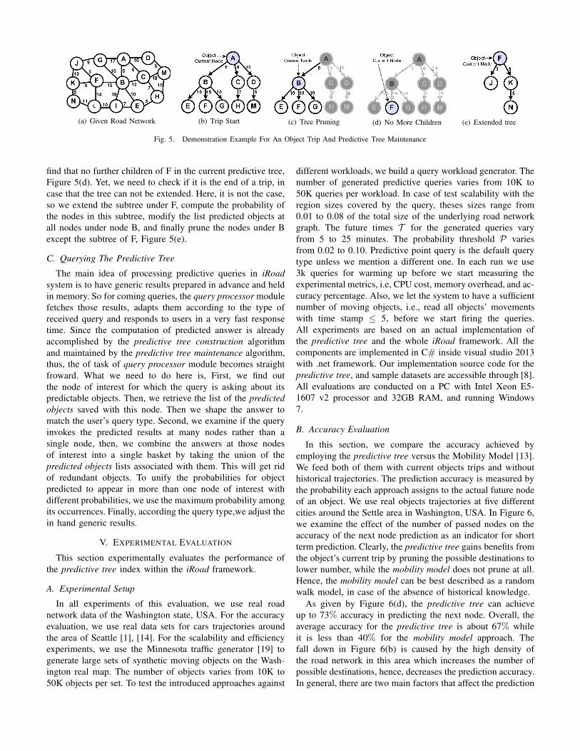
Example. Figure 5 illustrates how the tree maintenance

algorithm works. Given the road network graph shown in

Figure 5(a), and assuming that the object o has started its trip

at node A, we construct its predictive tree rooted at node A and

its depth is 20 minutes, Figure 5(b). When the object o moves

to the next node B in its trip, then the algorithm preforms

some consequent actions, Figure 5(c). First, it assures that the

depth of the tree under the object current node B is at least

equal to the maximum prediction time T , which is valid in

this step. Second, it updates the list of predicted objects in all

nodes in the original tree rooted at node A. This is done by

modifying the probability at nodes B, E, F, and G, and deleting

the occurrence of o at nodes A, C, D, H, and M as they are

no longer possible destinations to o. Third, we prune the tree

by cutting off all nodes that are not possible destination to

o via a shortest path from start node A. So, we exclude the

nodes A, C, D, H, and M. This step reduces the CPU cost

required later to compute and update the probability at each

reachable node. As the object o travels to the next node F, we

(a) Given Road Network (b) Trip Start (c) Tree Pruning (d) No More Children (e) Extended tree

Fig. 5. Demonstration Example For An Object Trip And Predictive Tree Maintenance

find that no further children of F in the current predictive tree,

Figure 5(d). Yet, we need to check if it is the end of a trip, in

case that the tree can not be extended. Here, it is not the case,

so we extend the subtree under F, compute the probability of

the nodes in this subtree, modify the list predicted objects at

all nodes under node B, and finally prune the nodes under B

except the subtree of F, Figure 5(e).

C. Querying The Predictive Tree

The main idea of processing predictive queries in iRoad

system is to have generic results prepared in advance and held

in memory. So for coming queries, the query processor module

fetches those results, adapts them according to the type of

received query and responds to users in a very fast response

time. Since the computation of predicted answer is already

accomplished by the predictive tree construction algorithm

and maintained by the predictive tree maintenance algorithm,

thus, the of task of query processor module becomes straight

froward. What we need to do here is, First, we find out

the node of interest for which the query is asking about its

predictable objects. Then, we retrieve the list of the predicted

objects saved with this node. Then we shape the answer to

match the user’s query type. Second, we examine if the query

invokes the predicted results at many nodes rather than a

single node, then, we combine the answers at those nodes

of interest into a single basket by taking the union of the

predicted objects lists associated with them. This will get rid

of redundant objects. To unify the probabilities for object

predicted to appear in more than one node of interest with

different probabilities, we use the maximum probability among

its occurrences. Finally, according the query type,we adjust the

in hand generic results.

V. EXPERIMENTAL EVALUATION

This section experimentally evaluates the performance of

the predictive tree index within the iRoad framework.

A. Experimental Setup

In all experiments of this evaluation, we use real road

network data of the Washington state, USA. For the accuracy

evaluation, we use real data sets for cars trajectories around

the area of Seattle [1], [14]. For the scalability and efficiency

experiments, we use the Minnesota traffic generator [19] to

generate large sets of synthetic moving objects on the Wash-

ington real map. The number of objects varies from 10K to

50K objects per set. To test the introduced approaches against

different workloads, we build a query workload generator. The

number of generated predictive queries varies from 10K to

50K queries per workload. In case of test scalability with the

region sizes covered by the query, theses sizes range from

0.01 to 0.08 of the total size of the underlying road network

graph. The future times T for the generated queries vary

from 5 to 25 minutes. The probability threshold P varies

from 0.02 to 0.10. Predictive point query is the default query

type unless we mention a different one. In each run we use

3k queries for warming up before we start measuring the

experimental metrics, i.e, CPU cost, memory overhead, and ac-

curacy percentage. Also, we let the system to have a sufficient

number of moving objects, i.e., read all objects’ movements

with time stamp ≤ 5, before we start firing the queries.

All experiments are based on an actual implementation of

the predictive tree and the whole iRoad framework. All the

components are implemented in C# inside visual studio 2013

with .net framework. Our implementation source code for the

predictive tree, and sample datasets are accessible through [8].

All evaluations are conducted on a PC with Intel Xeon E5-

1607 v2 processor and 32GB RAM, and running Windows

7.

B. Accuracy Evaluation

In this section, we compare the accuracy achieved by

employing the predictive tree versus the Mobility Model [13].

We feed both of them with current objects trips and without

historical trajectories. The prediction accuracy is measured by

the probability each approach assigns to the actual future node

of an object. We use real objects trajectories at five different

cities around the Settle area in Washington, USA. In Figure 6,

we examine the effect of the number of passed nodes on the

accuracy of the next node prediction as an indicator for short

term prediction. Clearly, the predictive tree gains benefits from

the object’s current trip by pruning the possible destinations to

lower number, while the mobility model does not prune at all.

Hence, the mobility model can be best described as a random

walk model, in case of the absence of historical knowledge.

As given by Figure 6(d), the predictive tree can achieve

up to 73% accuracy in predicting the next node. Overall, the

average accuracy for the predictive tree is about 67% while

it is less than 40% for the mobility model approach. The

fall down in Figure 6(b) is caused by the high density of

the road network in this area which increases the number of

possible destinations, hence, decreases the prediction accuracy.

In general, there are two main factors that affect the prediction

0

0.2

0.4

0.6

0.8

1

0 1 2 3 4 5 6

AV

G P

rob

ab

ilit

y

Passed Nodes

Predictive TreeMobility Model

(a) Endmonds

0

0.2

0.4

0.6

0.8

1

0 1 2 3 4 5 6

AV

G P

rob

ab

ilit

y

Passed Nodes

Predictive TreeMobility Model

(b) Ravenna

0

0.2

0.4

0.6

0.8

1

0 1 2 3 4 5 6

AV

G P

rob

ab

ilit

y

Passed Nodes

Predictive TreeMobility Model

(c) Bellevue

0

0.2

0.4

0.6

0.8

1

0 1 2 3 4 5 6

AV

G P

rob

ab

ilit

y

Passed Nodes

Predictive TreeMobility Model

(d) Redmond

0

0.2

0.4

0.6

0.8

1

0 1 2 3 4 5 6

AV

G P

rob

ab

ilit

y

Passed Nodes

Predictive TreeMobility Model

(e) Kenmore

Fig. 6. Accuracy Evaluation For Short Term Prediction

0

0.2

0.4

0.6

0.8

1

1 2 3 4 5

AV

G P

rob

ab

ilit

y

Next Nodes

Predictive TreeMobility Model

(a) Endmonds

0

0.2

0.4

0.6

0.8

1

1 2 3 4 5

AV

G P

rob

ab

ilit

y

Next Nodes

Predictive TreeMobility Model

(b) Ravenna

0

0.2

0.4

0.6

0.8

1

1 2 3 4 5

AV

G P

rob

ab

ilit

y

Next Nodes

Predictive TreeMobility Model

(c) Bellevue

0

0.2

0.4

0.6

0.8

1

1 2 3 4 5

AV

G P

rob

ab

ilit

y

Next Nodes

Predictive TreeMobility Model

(d) Redmond

0

0.2

0.4

0.6

0.8

1

1 2 3 4 5

AV

G P

rob

ab

ilit

y

Next Nodes

Predictive TreeMobility Model

(e) Kenmore

Fig. 7. Accuracy Evaluation For Long Term Prediction

accuracy inside the predictive tree . (1) The extent to which a

moving object follows the shortest paths in its travel, and (2)

the average degree of a node in the underlying road network.

In attempt to test the accuracy pattern of each approach in long

term prediction, we let the objects pass by a sufficient number

of nodes, i.e., five nodes, then we measure the probability

given to each of the five nodes next to the objects’ current

node, Figure 7. As expected, the accuracy decreases while we

look far in the future. However, the predictive tree still acts

better.

C. Scalability Evaluation

For the scalability evaluation, we compare the two different

approaches, precomputed and on-demand, of employing the

predictive tree inside the iRaod framework. As discussed in

Section III, the earlier is the default approach inside the

iRoad framework where the predicted objects are computed

and stored at each node in advance. While in the latest,

we postpone all computations until a query is received. In

these sets of experiments, we study the scalability of the

predictive tree within the two aforementioned approaches with

numbers of queries, query sizes, i.e., for predictive range

queries, number of moving objects, future prediction time T ,

and different levels of the probability threshold P . For each

test, we measure the average CPU time and the maximum

memory footprint.

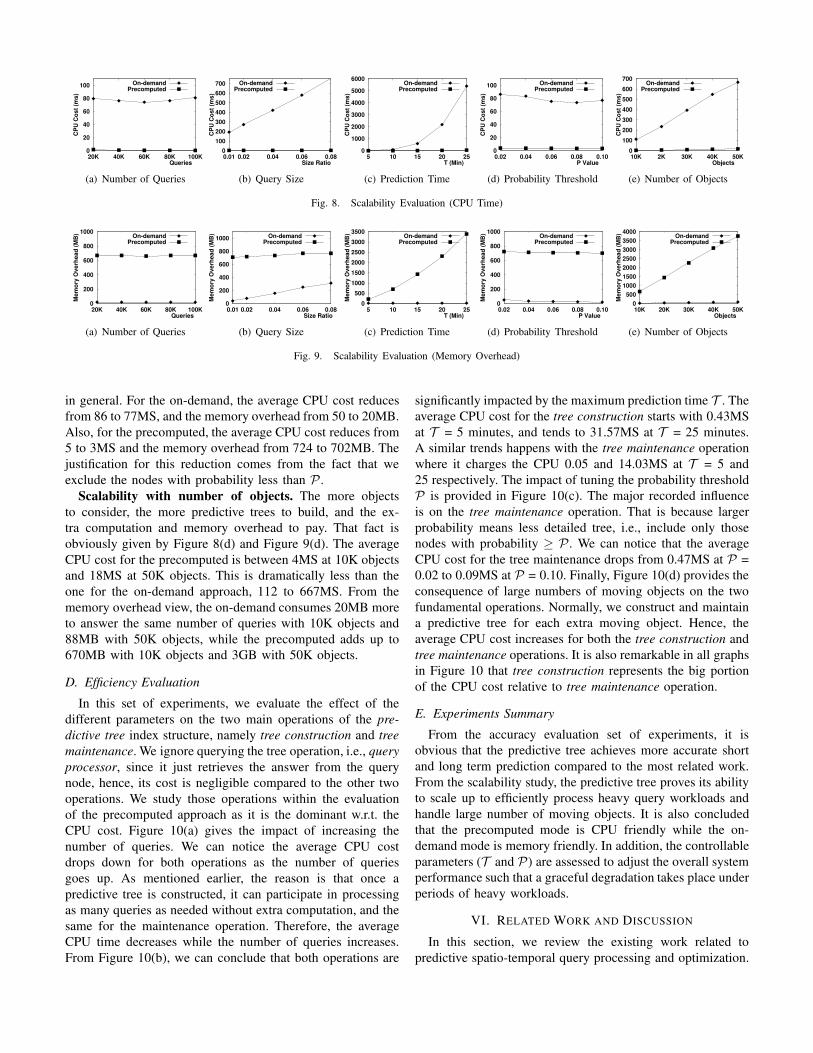
Scalability with number of queries. As depicted in

Figure 8(a), the CPU cost for the on-demand approach is

almost steady around 75 millisecond per query. While for

the precomputed approach, it decreases from 8 millisecond

per query to less than half millisecond when the number of

queries increases from 20K to 100K. This concludes that the

precomputed approach significantly saves the CPU time. The

reason is that once we compute and save the predicted answer

at a node, it serves as many queries as needed without extra

computation. However, the on-demand approach acts better

w.r.t. memory overhead, Figure 9(a), as it does empty the data

structures once the query is processed.

Scalability with query size. In this set of experiments, we

study the scalability of each approach with large query sizes

in predictive range queries. We vary the query size ratio from

0.01 to 0.08 of the the given road network graph. We found

that the average CPU cost per query for the precomputed

is almost steady at 3MS, while it varies from 194MS to

755MS for the on-demand. This means the CPU cost for the

on-demand approach linearly increases when the query size

increases, Figure 8(b). Intuitively, this is a rational behavior, as

the on-demand performs computations for more objects with

bigger sizes. Obviously, from the CPU time perspective, the

precomputed approach is faster by orders of magnitude. From

the memory overhead perspective, Figure 9(b), the on-demand

approach is more memory friendly. However, it has some

slightly increasing trend as a result of keeping the predictive

trees longer time till the query is processed as a whole.

Scalability with prediction time T . When we examine the

scalability with the maximum prediction time T the predictive

tree can support, we can notice a remarkable increase in

both approaches w.r.t. the average CPU cost, Figure 8(c).

However, there is a significant difference between the mini-

mum/maximum CPU cost for each approach. The lowest CPU

cost for the precomputed approach is 0.5MS at T = 5 minutes

and 2MS for the on-demand, while the maximum is 45MS and

5395MS respectively at T = 25 minutes. The CPU time over-

heads come from the extra computations required to construct

bigger predictive trees and maintain more reachable nodes.

On the other hand, the memory overhead for the on-demand

is almost stationary, i.e., from 19 to 22MB. This is extremely

less than the min/max overheads for the precomputed, i.e.,

219MB and 3.4GB, Figure 9(c).

Scalability with probability threshold P . Figure 8(d) and

Figure 9(d) illustrate the effect of increasing the probability

threshold P from 0.02 to 0.10 on the scalability of the iRoad

0

20

40

60

80

100

20K 40K 60K 80K 100K

CP

U C

os

t (m

s)

Queries

On-demandPrecomputed

(a) Number of Queries

0

100

200

300

400

500

600

700

0.01 0.02 0.04 0.06 0.08

CP

U C

os

t (m

s)

Size Ratio

On-demandPrecomputed

(b) Query Size

0

1000

2000

3000

4000

5000

6000

5 10 15 20 25

CP

U C

os

t (m

s)

T (Min)

On-demandPrecomputed

(c) Prediction Time

0

20

40

60

80

100

0.02 0.04 0.06 0.08 0.10

CP

U C

os

t (m

s)

P Value

On-demandPrecomputed

(d) Probability Threshold

0

100

200

300

400

500

600

700

10K 2K 30K 40K 50K

CP

U C

os

t (m

s)

Objects

On-demandPrecomputed

(e) Number of Objects

Fig. 8. Scalability Evaluation (CPU Time)

0

200

400

600

800

1000

20K 40K 60K 80K 100K

Me

mo

ry O

ve

rhe

ad

(M

B)

Queries

On-demandPrecomputed

(a) Number of Queries

0

200

400

600

800

1000

0.01 0.02 0.04 0.06 0.08

Me

mo

ry O

ve

rhe

ad

(M

B)

Size Ratio

On-demandPrecomputed

(b) Query Size

0

500

1000

1500

2000

2500

3000

3500

5 10 15 20 25

Me

mo

ry O

ve

rhe

ad

(M

B)

T (Min)

On-demandPrecomputed

(c) Prediction Time

0

200

400

600

800

1000

0.02 0.04 0.06 0.08 0.10

Me

mo

ry O

ve

rhe

ad

(M

B)

P Value

On-demandPrecomputed

(d) Probability Threshold

0

500

1000

1500

2000

2500

3000

3500

4000

10K 20K 30K 40K 50K

Me

mo

ry O

ve

rhe

ad

(M

B)

Objects

On-demandPrecomputed

(e) Number of Objects

Fig. 9. Scalability Evaluation (Memory Overhead)

in general. For the on-demand, the average CPU cost reduces

from 86 to 77MS, and the memory overhead from 50 to 20MB.

Also, for the precomputed, the average CPU cost reduces from

5 to 3MS and the memory overhead from 724 to 702MB. The

justification for this reduction comes from the fact that we

exclude the nodes with probability less than P .

Scalability with number of objects. The more objects

to consider, the more predictive trees to build, and the ex-

tra computation and memory overhead to pay. That fact is

obviously given by Figure 8(d) and Figure 9(d). The average

CPU cost for the precomputed is between 4MS at 10K objects

and 18MS at 50K objects. This is dramatically less than the

one for the on-demand approach, 112 to 667MS. From the

memory overhead view, the on-demand consumes 20MB more

to answer the same number of queries with 10K objects and

88MB with 50K objects, while the precomputed adds up to

670MB with 10K objects and 3GB with 50K objects.

D. Efficiency Evaluation

In this set of experiments, we evaluate the effect of the

different parameters on the two main operations of the pre-

dictive tree index structure, namely tree construction and tree

maintenance. We ignore querying the tree operation, i.e., query

processor, since it just retrieves the answer from the query

node, hence, its cost is negligible compared to the other two

operations. We study those operations within the evaluation

of the precomputed approach as it is the dominant w.r.t. the

CPU cost. Figure 10(a) gives the impact of increasing the

number of queries. We can notice the average CPU cost

drops down for both operations as the number of queries

goes up. As mentioned earlier, the reason is that once a

predictive tree is constructed, it can participate in processing

as many queries as needed without extra computation, and the

same for the maintenance operation. Therefore, the average

CPU time decreases while the number of queries increases.

From Figure 10(b), we can conclude that both operations are

significantly impacted by the maximum prediction time T . The

average CPU cost for the tree construction starts with 0.43MS

at T = 5 minutes, and tends to 31.57MS at T = 25 minutes.

A similar trends happens with the tree maintenance operation

where it charges the CPU 0.05 and 14.03MS at T = 5 and

25 respectively. The impact of tuning the probability threshold

P is provided in Figure 10(c). The major recorded influence

is on the tree maintenance operation. That is because larger

probability means less detailed tree, i.e., include only those

nodes with probability ≥ P . We can notice that the average

CPU cost for the tree maintenance drops from 0.47MS at P =

0.02 to 0.09MS at P = 0.10. Finally, Figure 10(d) provides the

consequence of large numbers of moving objects on the two

fundamental operations. Normally, we construct and maintain

a predictive tree for each extra moving object. Hence, the

average CPU cost increases for both the tree construction and

tree maintenance operations. It is also remarkable in all graphs

in Figure 10 that tree construction represents the big portion

of the CPU cost relative to tree maintenance operation.

E. Experiments Summary

From the accuracy evaluation set of experiments, it is

obvious that the predictive tree achieves more accurate short

and long term prediction compared to the most related work.

From the scalability study, the predictive tree proves its ability

to scale up to efficiently process heavy query workloads and

handle large number of moving objects. It is also concluded

that the precomputed mode is CPU friendly while the on-

demand mode is memory friendly. In addition, the controllable

parameters (T and P) are assessed to adjust the overall system

performance such that a graceful degradation takes place under

periods of heavy workloads.

VI. RELATED WORK AND DISCUSSION

In this section, we review the existing work related to

predictive spatio-temporal query processing and optimization.

0

0.4

0.8

1.2

1.6

2

20K 30K 40K 60K 80K 100K

CP

U T

ime

(M

S)

Queries

Tree ConstructionTree Maintenance

(a) Number of Queries

0

10

20

30

40

50

60

70

80

5 10 15 20 25 30

CP

U T

ime

(M

S)

T (Min)

Tree ConstructionTree Maintenance

(b) Prediction Time

0

1

2

3

4

5

0.02 0.04 0.06 0.08 0.10

CP

U T

ime

(M

S)

P Value

Tree ConstructionTree Maintenance

(c) Probability Threshold

0

4

8

12

16

20

10K 20K 30K 40K 50K

CP

U T

ime

(M

S)

Objects

Tree ConstructionTree Maintenance

(d) Number of Objects

Fig. 10. Efficiency Evaluation Of Main Operations In The Predictive Tree

Then, we summarize the related prediction models for moving

objects. This review of related work leads us to the question of

how the predictive tree fits in the bigger umbrella of spatio-

temporal query processing, how it is different from existing

techniques and, more interestingly, how it would complement

and integrate with the existing predictive query processing

techniques and prediction models.

A. Predictive Spatio-temporal Query Processing

Existing algorithms for predictive query processing can be

classified, according to the query type, into the following

categories:

(1) Range queries, i.e., [13], [25], [30]. A predictive range

query has a query region R and a future time window T ,

and asks about the objects that are expected to be inside R

within the time window T . A mobility model [13] is used

to predict the path of each underlying moving object that is

being monitored by the system. Most existing work considers

the query region to be a rectangle. However, the Transformed

Minkowski Sum is used to address circular region ranges [30].

(2) K-nearest-neighbor queries, i.e., [3], [22], [30]. A pre-

dictive K-nearest-neighbor query has a point location P and a

future time window T , and asks about the K objects expected

to be closest to P within the time window T . Two algo-

rithms, RangeSearch and KNNSearchBF [30], are introduced

to traverse a spatio-temporal index tree (the TPR/TPR∗-tree)

to answer range and KNN queries, respectively. Sometimes an

expiry time interval is attached to a kNN query result [26], [27]

to indicate the future time window during which the answer

is valid.

(3) Aggregate queries, i.e., [2], [9], [24]. A predictive

aggregate query has a query region R and a future time

window T , and asks about the number of objects N expected

to be inside R within the time window T . The approximate

query processing approach in [24] employs an adaptive multi-

dimensional histogram (AMH), a historical synopsis, and a

stochastic method to provide an approximate answer for aggre-

gate spatio-temporal queries about the future in addition to the

past and the present. A generic query processing framework

named Panda [9] is introduced to evaluate predictive queries

for moving objects on Euclidean space.

B. Prediction Models

In fact, many prediction models have been proposed to

predict the next movements of an object. One group of these

prediction models are based on the Euclidean space, e.g., [9],

[28], [25], [30], where objects can move freely in the two

dimensional space without any constrains, i.e., without being

restricted to move over edges of a road network. Furthermore,

these models use Euclidean distance rather than the cost to

traverse an edge within a road network graph.

Another group of prediction models that consider move-

ments on road networks has been recently proposed, e.g., [12],

[13]. The basic idea in these models is to calculate a turning

probability based on applying some data mining and statistical

techniques, i.e., association rules and decision trees, on the

objects’ historical trajectories. These models suffer from the

following drawbacks: 1) The process of building a predication

model requires large amount of historical trajectories, which

may not be available due to privacy concerns or lack of

coverage in rural areas. 2) Dispatching a data mining based

model in a system that serves millions of objects places a

significant overhead on computation and memory resources.

Hence, responsiveness to changes in the moving objects pat-

terns may be slow.

C. Discussion

To summarize, we would like to discuss how the predic-

tive tree fits under the bigger umbrella of predictive spatio-

temporal query processing and how it complements the wealth

of existing techniques discussed earlier in this section. More

specifically, we emphasize the following characteristics.

First, the predictive tree is a generic index structure in the

sense that it is neither built for a single type of predictive

queries nor for a single query processing algorithm. Rather,

it provides a shared infrastructure for evaluating various types

of predictive queries using various algorithms.

Second, many of the aforementioned techniques inherently

depend on the object’s past trajectory to accomplish the job. In

the absence of such historical trajectories, the predictive tree

provides a basis for these techniques to start with a predicted

trajectory that is computed solely using the connectivity of

the road network and, then, enhance the prediction quality

as more historical data becomes available. Consequently, the

aforementioned techniques are invited to utilize the predictive

tree in the absence of historical data.

Third, while some of the previously mentioned systems

are limited to the Euclidean space, the predictive tree is

designed to handle predictive spatio-temporal queries on road

networks. All computations are based on the underlying road

map structure, i.e., using the cost of edges in the road network

rather than the Euclidean distance.

Finally, the dynamic nature of the predictive tree and its

incremental maintenance approach lend the proposed index

naturally to the continuous query paradigm where low latency

response over high rate input streams is a system priority.

VII. CONCLUSION

In this paper, we presented the predictive tree, an index

structure to handle predictive queries against moving objects

on road networks. The predictive tree has been designed to

offer a generic framework for a set of predictive query types,

e.g., point, range and KNN predictive queries. The predictive

tree also offers an extensibility mechanism to integrate user

defined prediction models. The basic prediction model com-

putes the moving objects expected location solely based on the

connectivity of road network graph without need for objects’

previous trajectories. Yet, the user can extend the prediction

model to take into consideration historical trajectories of

moving objects or alter the probability assignment function ac-

cording to the application scenario. With the expected growth

in the number of moving objects, thanks to hand-held devices

and mobile phones, the predictive tree enables location-based

services to scale in terms of the number of predictive queries

against these moving objects. The incremental maintenance of

the predictive tree guarantees minimal processing of location

updates. Moreover, the behavior of the predictive tree is ad-

justed using a couple of tuning parameters that trade prediction

accuracy for system resources, i.e., memory and CPU. The

predictive tree has been implemented in the context of the

iRoad system. Empirical studies proved the scalability and

accuracy of the predictive tree.

REFERENCES

[1] M. Ali, J. Krumm, and A. Teredesai. ACM SIGSPATIAL GIS Cup 2012.In Proceedings of the ACM SIGSPATIAL International Conference on

Advances in Geographic Information Systems, ACM SIGSPATIAL GIS,pages 597–600, California, USA, Nov. 2012.

[2] S. Ayhan, J. Pesce, P. Comitz, G. Gerberick, and S. Bliesner. Pre-dictive Analytics with Aviation Big Data. In Proceeding of the ACM

SIGSPATIAL International Workshop on Analytics for Big Geospatial

Data, BigSpatial, California, USA, Nov. 2012.

[3] R. Benetis, C. S. Jensen, G. Karciauskas, and S. Saltenis. Nearest andReverse Nearest Neighbor Queries for Moving Objects. VLDB Journal,15(3):229–249, 2006.

[4] T. Brinkhoff. A Framework for Generating Network-Based MovingObjects. International Journal on Advances of Computer Science forGeographic Information Systems, GeoInformatica, 6(2):153–180, 2002.

[5] Y. Gu, G. Yu, N. Guo, and Y. Chen. Probabilistic Moving RangeQuery over RFID Spatio-temporal Data Streams. In Proceedings of the

International Conference on Information and Knowledge Managemen,

CIKM, pages 1413–1416, Hong Kong, China, Nov. 2009.

[6] G. Gulf. Smartphone Users Around the World Statistics and Facts.http://www.go-gulf.com/blog/smartphone/, Jan. 2012.

[7] Guttman and Antonin. R-trees: A Dynamic Index Structure for SpatialSearching. In Proceedings of the ACM International Conference on

Management of Data, SIGMOD, pages 47–57, Massachusetts, USA,June 1984.

[8] A. M. Hendawi, J. Bao, and M. F. Mokbel. Predictive Tree SourceCode and Sample Data. URL:http://www-users.cs.umn.edu/∼hendawi/PredictiveTree/, Aug. 2014.

[9] A. M. Hendawi and M. F. Mokbel. Panda: A Predictive Spatio-TemporalQuery Processor. In Proceedings of the ACM SIGSPATIAL International

Conference on Advances in Geographic Information Systems, ACM

SIGSPATIAL GIS, California, USA, Nov. 2012.[10] A. M. Hendawi and M. F. Mokbel. Predictive Spatio-Temporal Queries:

A Comprehensive Survey and Future Directions. In Proceeding of the

ACM SIGSPATIAL GIS International Workshop on Mobile Geographic

Information Systems, MobiGIS, California, USA, Nov. 2012.[11] H. Hu, J. Xu, and D. L. Lee. A Generic Framework for Monitoring

Continuous Spatial Queries over Moving Objects. In Proceedings of

the ACM International Conference on Management of Data, SIGMOD,pages 479–490, Maryland, USA, June 2005.

[12] H. Jeung, Q. Liu, H. T. Shen, and X. Zhou. A Hybrid Prediction Modelfor Moving Objects. In Proceedings of the International Conference on

Data Engineering, ICDE, pages 70–79, Cancn, Mxico, Apr. 2008.[13] H. Jeung, M. L. Yiu, X. Zhou, and C. S. Jensen. Path Prediction and

Predictive Range Querying in Road Network Databases. VLDB Journal,19(4):585–602, Aug. 2010.

[14] JOSM. An extensible editor for OpenStreetMap (OSM). http://josm.openstreetmap.de/wiki, Jan. 2014.

[15] H. A. Karimi and X. Liu. A Predictive Location Model for Location-Based Services. In Proceedings of the ACM Symposium on Advances inGeographic Information Systems, ACM GIS, pages 126–133, Louisiana,USA, Nov. 2003.

[16] J. Krumm. Real Time Destination Prediction Based on Efficient Routes.In Proceedings of the Society of Automotive Engineers World Congress,SAE, Michigan, USA, Apr. 2006.

[17] J. Krumm. How People Use Their Vehicles: Statistics from the 2009National Household Travel Survey. In Proceedings of the Society of

Automotive Engineers World Congress, SAE, Michigan, USA, Apr. 2008.[18] J. Krumm, R. Gruen, and D. Delling. From Destiantion Prediction To

Route Prediction. Technical Report. Microsoft Research, 2011.[19] M. F. Mokbel, L. Alarabi, J. Bao, A. Eldawy, A. Magdy, M. Sarwat,

E. Waytas, and S. Yackel. MNTG: An Extensible Web-based TrafficGenerator. In Proceedings of the International Symposium on Advances

in Spatial and Temporal Databases, SSTD, pages 38–55, Munich,Germany, Aug. 2013.

[20] M. F. Mokbel, X. Xiong, M. A. Hammad, and W. G. Aref. ContinuousQuery Processing of Spatio-temporal Data Streams in PLACE. GeoIn-

formatica, 9(4):343–365, Dec. 2005.[21] D. Papadias, J. Zhang, and N. Mamoulis. Query Processing in Spatial

Network Databases. In Proceedings of the International Conference on

Very Large Data Bases, VLDB, pages 802–813, Berlin, Germany, Sept.2003.

[22] K. Raptopoulou, A. Papadopoulos, and Y. Manolopoulos. Fast Nearest-Neighbor Query Processing in Moving-Object Databases. GeoInformat-

ica, 7(2):113–137, June 2003.[23] Stanford. Large Network Dataset Collection. http://snap.stanford.edu/

data/#road, Jan. 2013.[24] J. Sun, D. Papadias, Y. Tao, and B. Liu. Querying about the Past,

the Present, and the Future in Spatio-Temporal. In Proceedings of theInternational Conference on Data Engineering, ICDE, pages 202–213,MASSACHUSETTS, USA, Mar. 2004.

[25] Y. Tao, C. Faloutsos, D. Papadias, and B. L. 0002. Prediction andIndexing of Moving Objects with Unknown Motion Patterns. InProceedings of the ACM International Conference on Management of

Data, SIGMOD, pages 611–622, Paris, France, June 2004.[26] Y. Tao and D. Papadias. Time-parameterized Queries in Spatio-temporal

Databases. In Proceedings of the ACM International Conference on

Management of Data, SIGMOD, pages 334–345, Wisconsin, USA, June2002.

[27] Y. Tao and D. Papadias. Spatial queries in dynamic environments. ACMTransactions on Database Systems, TODS, 28(2):101–139, 2003.

[28] Y. Tao, D. Papadias, and J. Sun. The TPR*-tree: An Optimized Spatio-Temporal Access Method for Predictive Queries. In Proceedings of theInternational Conference on Very Large Data Bases, VLDB, pages 790–801, Berlin, Germany, Sept. 2003.

[29] H. Wang, R. Zimmermann, and W.-S. Ku. Distributed ContinuousRange Query Processing on Moving Objects. In Proceedings of theInternational Conference on Database and Expert Systems Applications,

DEXA, pages 655–665, Krakow, Poland, Sept. 2006.[30] R. Zhang, H. V. Jagadish, B. T. Dai, and K. Ramamohanarao. Optimized

Algorithms for Predictive Range and KNN Queries on Moving Objects.Information Systems, 35(8):911–932, Dec. 2010.