The plastics engineer working on the shop floor of an industry manufacturing blown film or blow-molded articles or injection-molded parts, to quote a few processes, needs often quick answers to questions such as why the extruder output is low or whether he can expect better quality product by changing the resin or how he can estimate the pressure drop along the runner or gate of an injection mold. Applying the state of the art numerical analysis to address these issues is time-consuming and costly requiring trained personnel. Indeed, as experience shows, most of these issues can be addressed quickly by applying proven, practical calculation procedures which can be handled by pocket calculators and hence can be performed right on the site where the machines are running.
The underlying principles of design formulas for plastics engineers with examples have been treated in detail in the earlier works of Natti Rao.
Bridging the gap between theory and practice this book presents analytical methods based on these formulas which enable the plastics engineer to solve day to day problems related to machine design and process optimization quickly. Basically, the diagnostical approach used here lies in examining whether the machine design is suited to accomplish the desired process parameters.
Starting from solids transport, melting and moving on to shaping the melt in the die to create the product, this work shows the benefits of using simple analytical procedures for troubleshooting machinery and processes by verifying machine design first and then,if necessary, optimizing it to meet the process requirements. Illustrative examples chosen from rheology, heat transfer in plastics processing, extrusion screw and die design, blown film, extrusion coating and injection molding, to mention a few areas, clarify this approach in detail.
Case studies related to melt fracture, homogeneity of the melt, effect of extrusion screw geometry on the quality of the melt, classifying injection molding resins on the basis of their flow length and calculating runner and gate pressure drop are only a few of the topics among many, which have been treated in detail. In addition, parametric studies of blown film, pipe extrusion, extru-sion coating, sheet extrusion, thermoforming, and injection molding are presented, so that the user is acquainted with the process targets of the calculations.
X Preface
The same set of equations can be used to attain different targets whether they deal with extru-sion die design or injection molds. Practical calculations illustrate how a variety of goals can be reached by applying the given formulas along with the relevant examples.
In order to facilitate easy use, the formulas have been repeated in some calculations, so that the reader need not refer back to these formulas given elsewhere in the book.
This book is an example-based practical tool not only for estimating the effect of design and process parameters on the product quality but also for troubleshooting practical problems encountered in various fields of polymer processing. It is intended for beginners as well as for practicing engineers, students and teachers in the field of plastics engineering and also for scientists from other areas who deal with polymer engineering in their professions.
The Appendix contains a list of easily applicable computer programs for designing extrusion screws and dies. These can be obtained by contacting the author via email ([email protected]).
We are indebted to Dr. Guenter Schumacher of the European Joint Research Center, Ispra, Italy for his generous help in preparing the manuscript. Thanks are also due to Dr. Benjamin Dietrich of KIT, Karlsruhe, Germany for his cooperation in writing the manuscript. The fruitful discussions with Dr. Ranganath Shastri of CIATEQ Unidad Edomex, Mexico are thankfully acknowledged.
The permission of BASF SE for using the main library at Ludwigshafen Rhein, Germany is thankfully acknowledged by Natti S. Rao.
4 Analytical Procedures for Troubleshooting extrusion Screws
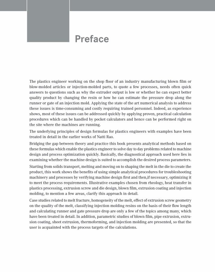
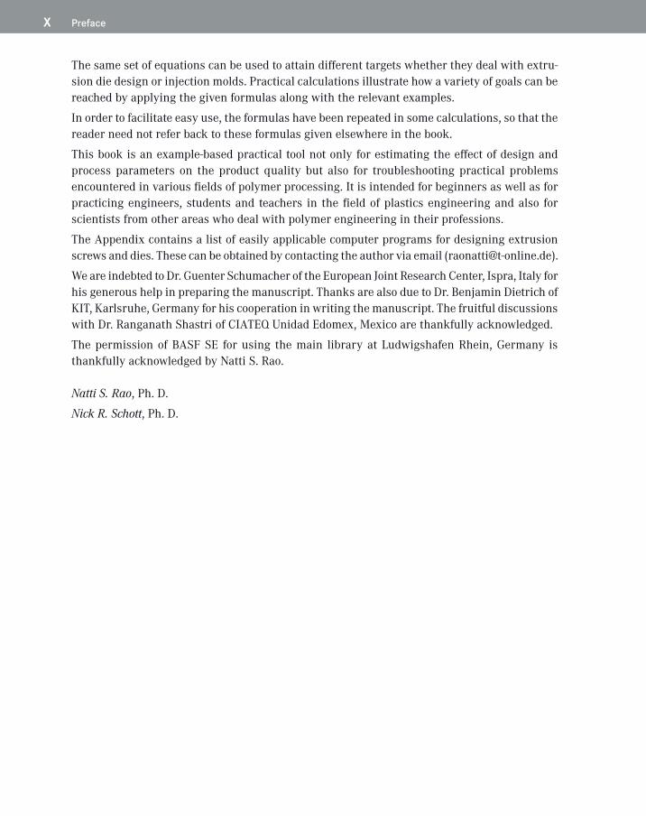
Extrusion is one of the most widely used polymer converting operations for manufacturing blown film, pipes, sheets, and laminations, to list the most significant industrial applications. Fig. 4.1 shows a modern large scale machine for making blown film. The extruder, which constitutes the central unit of these machines, is shown in Fig. 4.2. The polymer is fed into the hopper in the form of granulate or powder. It is kept at the desired temperature and humidity by controlled air circulation. The solids are conveyed by the rotating screw and slowly melted, in part, by barrel heating but mainly by the frictional heat generated by the shear between the polymer and the barrel (Fig. 4.3). The melt at the desired temperature and pressure flows through the die, in which the shaping of the melt into the desired shape takes place.
FIguRe 4.1 Large scale blown film line [2]
68 4 Analytical Procedures for Troubleshooting Extrusion Screws
FIguRe 4.2 Extruder with auxialiary equipment [3]
■ 4.1 Three-Zone Screw
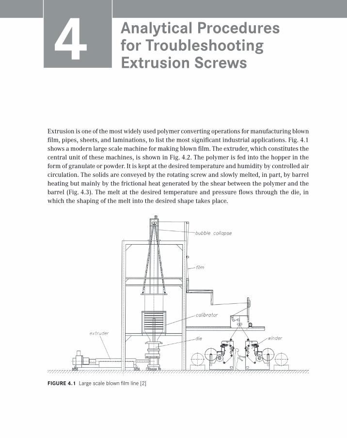
Basically extrusion consists of transporting the solid polymer in an extruder by means of a rotat-ing screw, melting the solid, homogenizing the melt, and forcing the melt through a die (Fig. 4.3).
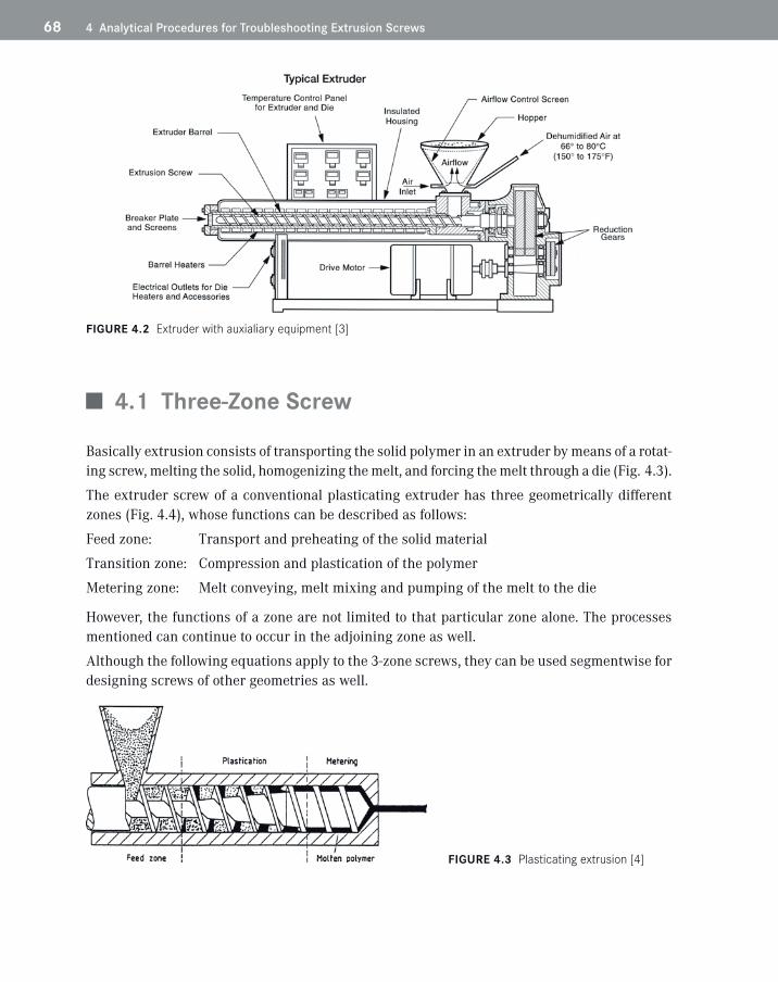
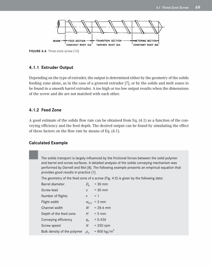
The extruder screw of a conventional plasticating extruder has three geometrically different zones (Fig. 4.4), whose functions can be described as follows:
Feed zone: Transport and preheating of the solid material
Transition zone: Compression and plastication of the polymer
Metering zone: Melt conveying, melt mixing and pumping of the melt to the die
However, the functions of a zone are not limited to that particular zone alone. The processes mentioned can continue to occur in the adjoining zone as well.
Although the following equations apply to the 3-zone screws, they can be used segmentwise for designing screws of other geometries as well.
FIguRe 4.3 Plasticating extrusion [4]
694.1 Three-Zone Screw
FIguRe 4.4 Three-zone screw [10]
4.1.1 extruder Output
Depending on the type of extruder, the output is determined either by the geometry of the solids feeding zone alone, as in the case of a grooved extruder [7], or by the solids and melt zones to be found in a smooth barrel extruder. A too high or too low output results when the dimensions of the screw and die are not matched with each other.
4.1.2 Feed Zone
A good estimate of the solids flow rate can be obtained from Eq. (4.1) as a function of the con-veying efficiency and the feed depth. The desired output can be found by simulating the effect of these factors on the flow rate by means of Eq. (4.1).
Calculated example
The solids transport is largely influenced by the frictional forces between the solid polymer and barrel and screw surfaces. A detailed analysis of the solids conveying mechanism was performed by Darnell and Mol [8]. The following example presents an empirical equation that provides good results in practice [1].The geometry of the feed zone of a screw (Fig. 4.5) is given by the following data:Barrel diameter Db = 30 mmScrew lead s = 30 mmNumber of flights = 1Flight width wFLT = 3 mmChannel width W = 28.6 mmDepth of the feed zone H = 5 mmConveying efficiency hF = 0.436Screw speed N = 250 rpmBulk density of the polymer ro = 800 kg/m3
70 4 Analytical Procedures for Troubleshooting Extrusion Screws
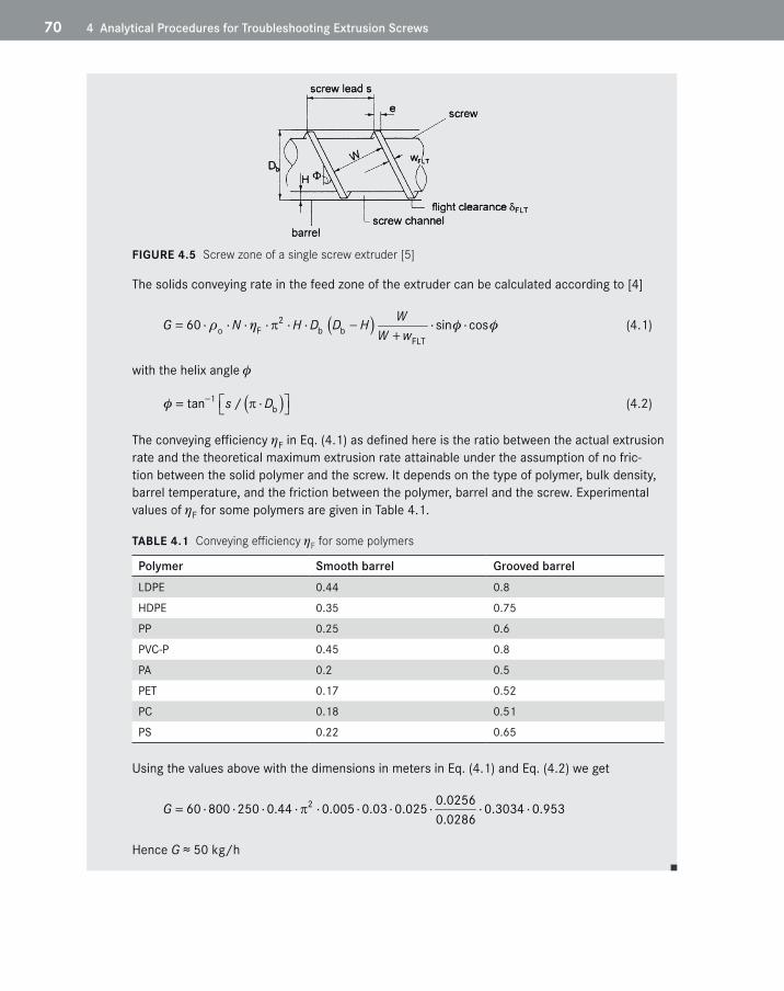
FIguRe 4.5 Screw zone of a single screw extruder [5]
The solids conveying rate in the feed zone of the extruder can be calculated according to [4]
( )r h π= ⋅ ⋅ ⋅ ⋅ ⋅ ⋅ − ⋅ ⋅+
2o F b b
FLT60 sin cosWG N H D D H
W w (4.1)
with the helix angle
( ) π− = ⋅ 1
btan /s D (4.2)
The conveying efficiency hF in Eq. (4.1) as defined here is the ratio between the actual extrusion rate and the theoretical maximum extrusion rate attainable under the assumption of no fric-tion between the solid polymer and the screw. It depends on the type of polymer, bulk density, barrel temperature, and the friction between the polymer, barrel and the screw. Experimental values of hF for some polymers are given in Table 4.1.
TAbLe 4.1 Conveying efficiency hF for some polymers
Polymer Smooth barrel Grooved barrelLDPE 0.44 0.8
HDPE 0.35 0.75
PP 0.25 0.6
PVC-P 0.45 0.8
PA 0.2 0.5
PET 0.17 0.52
PC 0.18 0.51
PS 0.22 0.65
Using the values above with the dimensions in meters in Eq. (4.1) and Eq. (4.2) we get
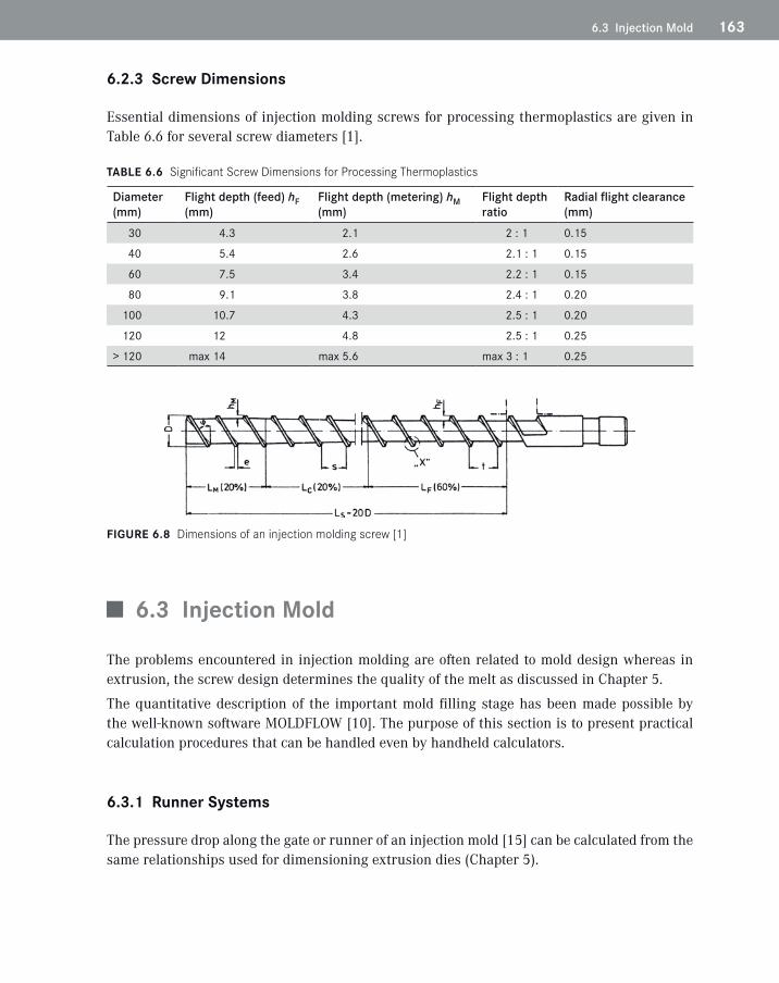
Essential dimensions of injection molding screws for processing thermoplastics are given in Table 6.6 for several screw diameters [1].
TAbLe 6.6 Significant Screw Dimensions for Processing Thermoplastics
Diameter(mm)
Flight depth (feed) hF(mm)
Flight depth (metering) hM(mm)
Flight depth ratio
Radial flight clearance(mm)
30 4.3 2.1 2 : 1 0.15
40 5.4 2.6 2.1 : 1 0.15
60 7.5 3.4 2.2 : 1 0.15
80 9.1 3.8 2.4 : 1 0.20
100 10.7 4.3 2.5 : 1 0.20
120 12 4.8 2.5 : 1 0.25
> 120 max 14 max 5.6 max 3 : 1 0.25
FIguRe 6.8 Dimensions of an injection molding screw [1]
■ 6.3 Injection Mold
The problems encountered in injection molding are often related to mold design whereas in extrusion, the screw design determines the quality of the melt as discussed in Chapter 5.
The quantitative description of the important mold filling stage has been made possible by the well-known software MOLDFLOW [10]. The purpose of this section is to present practical calculation procedures that can be handled even by handheld calculators.
6.3.1 Runner Systems
The pressure drop along the gate or runner of an injection mold [15] can be calculated from the same relationships used for dimensioning extrusion dies (Chapter 5).
164 6 Analytical Procedures for Troubleshooting Injection Molding
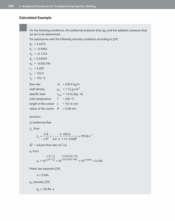
Calculated example
For the following conditions, the isothermal pressure drop Dp0 and the adiabatic pressure drop Dp are to be determined:For polystyrene with the following viscosity constants according to [29]A0 = 4.4475A1 = –0.4983A2 = –0.1743A3 = 0.03594A4 = –0.002196c1 = 4.285c2 = 133.2T0 = 190 °C
flow rate m = 330.4 kg/hmelt density rm = 1.12 g/cm3
specific heat cpm = 1.6 kJ/(kg · K)melt temperature T = 230 °Clength of the runner L = 101.6 mmradius of the runner R = 5.08 mm
Solution:
a) Isothermal flow
a from
π π
−⋅= = =⋅ ⋅ ⋅
1a 3 3
4 4 330.0 795.8 s3.6 1.12 0.508
QR
( Q = volume flow rate cm3/s)
aT from( )( )
( )( )
− − − −+ − + − −= = = =1 0
2 0
4.285 230 190133.2 230 190 0.9896
T 10 10 10 0.102
c T Tc T Ta
Power law exponent [29]
= 5.956n
ha, viscosity [29]
h = ⋅a 132 Pa s
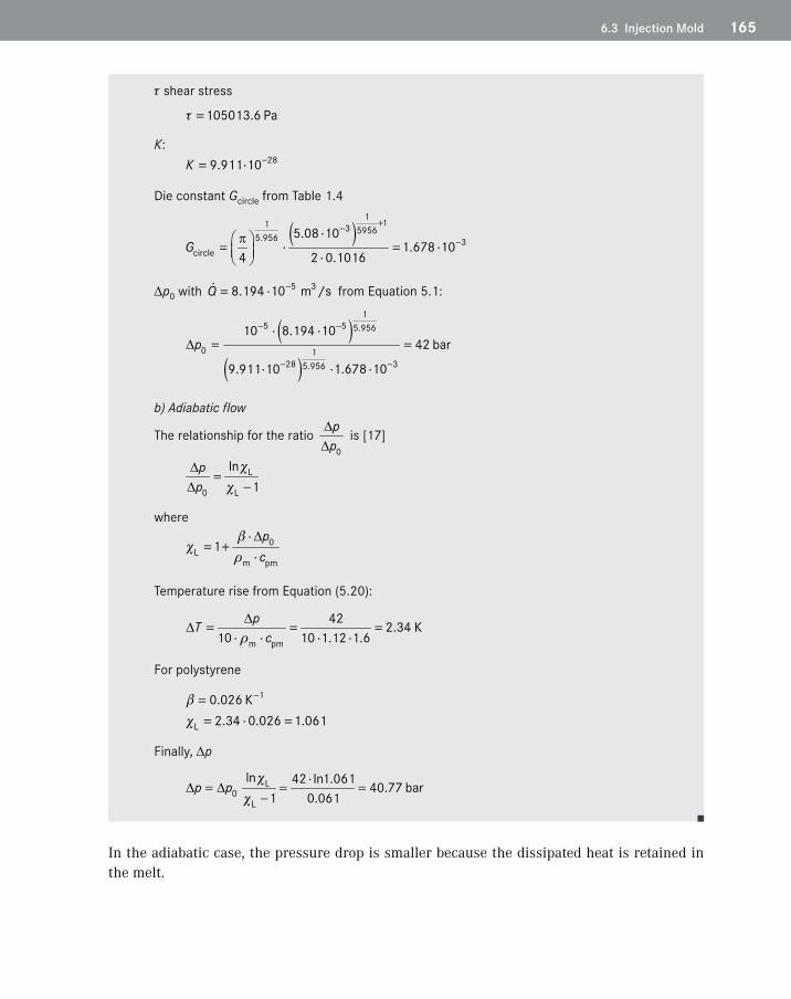
1656.3 Injection Mold
shear stress
=105013.6 Pa
K:−= ⋅ 289.911 10K
Die constant Gcircle from Table 1.4
( )π+−
−⋅
= ⋅ = ⋅ ⋅
1 11 3 59565.956 3
circle
5.08 101.678 10
4 2 0.1016G
Dp0 with −= ⋅
5 38.194 10 m /sQ from Equation 5.1:
( )( )
D− −
− −
⋅ ⋅= =
⋅ ⋅ ⋅
15 5 5.956
0 128 35.956
10 8.194 1042 bar
9.911 10 1.678 10
p
b) Adiabatic flow
The relationship for the ratio DD 0
pp
is [17]
DD
=−L
0 L
ln1
pp
where
r
D⋅= +
⋅0
Lm pm
1pc
Temperature rise from Equation (5.20):
rD
D = = =⋅ ⋅ ⋅ ⋅m pm
42 2.34 K10 10 1.12 1.6
pTc
For polystyrene
−== ⋅ =
1
L
0.026 K2.34 0.026 1.061
Finally, Dp
D D
⋅= = =−L
0L
ln 42 ln1.061 40.77 bar1 0.061
p p
In the adiabatic case, the pressure drop is smaller because the dissipated heat is retained in the melt.
166 6 Analytical Procedures for Troubleshooting Injection Molding
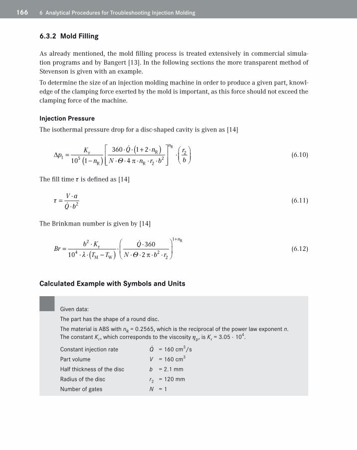
6.3.2 Mold Filling
As already mentioned, the mold filling process is treated extensively in commercial simula-tion programs and by Bangert [13]. In the following sections the more transparent method of Stevenson is given with an example.
To determine the size of an injection molding machine in order to produce a given part, knowl-edge of the clamping force exerted by the mold is important, as this force should not exceed the clamping force of the machine.
Injection PressureThe isothermal pressure drop for a disc-shaped cavity is given as [14]
( )( ) R
Rr 21 5 2
R R 2
360 1 2
10 1 4
nQ nK r
pbn N n r b
Dπ
⋅ ⋅ + ⋅ = ⋅ − ⋅ ⋅ ⋅ ⋅ ⋅ Θ
(6.10)
The fill time is defined as [14]
2V aQ b
⋅=⋅
(6.11)
The Brinkman number is given by [14]
( )R12
r4 2
M W 2
36010 2
nb K QBr
T T N b r π
+ ⋅ ⋅= ⋅ ⋅ ⋅ − ⋅ ⋅ ⋅ ⋅ Θ
(6.12)
Calculated example with Symbols and units
Given data:The part has the shape of a round disc.The material is ABS with nR = 0.2565, which is the reciprocal of the power law exponent n. The constant Kr, which corresponds to the viscosity hp, is Kr = 3.05 · 104.
Half thickness of the disc b = 2.1 mmRadius of the disc r2 = 120 mmNumber of gates N = 1
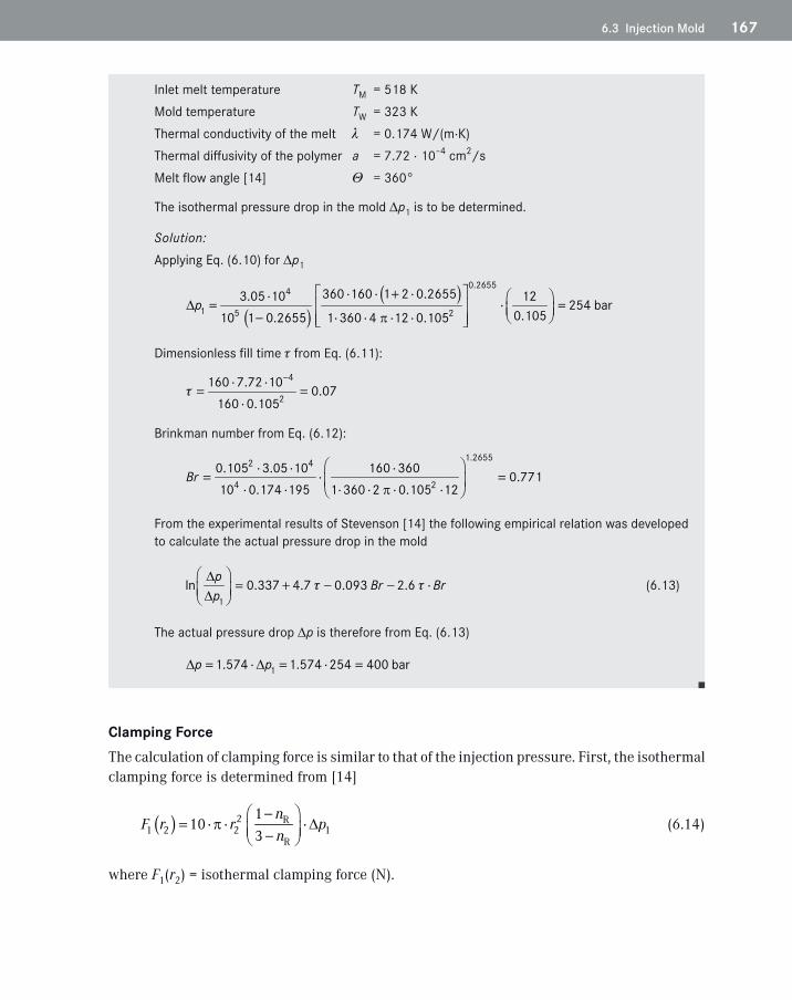
1676.3 Injection Mold
Inlet melt temperature TM = 518 KMold temperature TW = 323 KThermal conductivity of the melt = 0.174 W/(m·K)Thermal diffusivity of the polymer a = 7.72 · 10–4 cm2/sMelt flow angle [14] Θ = 360°
The isothermal pressure drop in the mold Dp1 is to be determined.
From the experimental results of Stevenson [14] the following empirical relation was developed to calculate the actual pressure drop in the mold
1ln 0.337 4.7 0.093 2.6p Br Br
p
DD
= + − − ⋅
(6.13)
The actual pressure drop Dp is therefore from Eq. (6.13)
11.574 1.574 254 400 barp pD D= ⋅ = ⋅ =
Clamping ForceThe calculation of clamping force is similar to that of the injection pressure. First, the isothermal clamping force is determined from [14]
( ) 2 R1 2 2 1
R
110
3n
F r r pn
π D −
= ⋅ ⋅ ⋅ − (6.14)
where F1(r2) = isothermal clamping force (N).
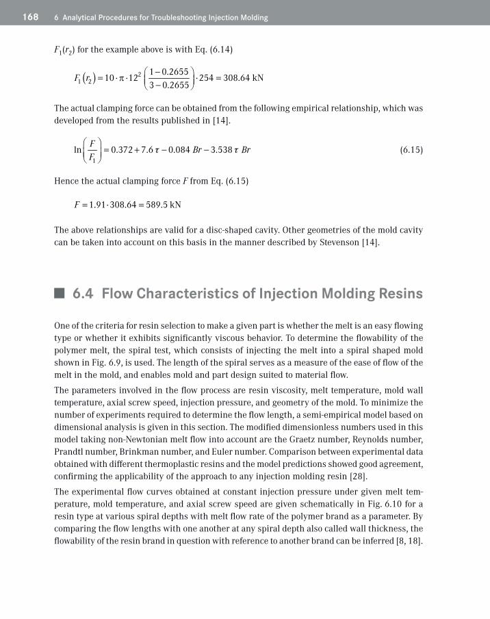
168 6 Analytical Procedures for Troubleshooting Injection Molding
F1(r2) for the example above is with Eq. (6.14)
( ) 21 2
1 0.265510 12 254 308.64 kN
3 0.2655F r π
− = ⋅ ⋅ ⋅ = −
The actual clamping force can be obtained from the following empirical relationship, which was developed from the results published in [14].
1ln 0.372 7.6 0.084 3.538
F Br BrF
= + − − (6.15)
Hence the actual clamping force F from Eq. (6.15)
1.91 308.64 589.5 kNF = ⋅ =
The above relationships are valid for a disc-shaped cavity. Other geometries of the mold cavity can be taken into account on this basis in the manner described by Stevenson [14].
■ 6.4 Flow Characteristics of Injection Molding Resins
One of the criteria for resin selection to make a given part is whether the melt is an easy flowing type or whether it exhibits significantly viscous behavior. To determine the flowability of the polymer melt, the spiral test, which consists of injecting the melt into a spiral shaped mold shown in Fig. 6.9, is used. The length of the spiral serves as a measure of the ease of flow of the melt in the mold, and enables mold and part design suited to material flow.
The parameters involved in the flow process are resin viscosity, melt temperature, mold wall temperature, axial screw speed, injection pressure, and geometry of the mold. To minimize the number of experiments required to determine the flow length, a semi-empirical model based on dimensional analysis is given in this section. The modified dimensionless numbers used in this model taking non-Newtonian melt flow into account are the Graetz number, Reynolds number, Prandtl number, Brinkman number, and Euler number. Comparison between experimental data obtained with different thermoplastic resins and the model predictions showed good agreement, confirming the applicability of the approach to any injection molding resin [28].
The experimental flow curves obtained at constant injection pressure under given melt tem-perature, mold temperature, and axial screw speed are given schematically in Fig. 6.10 for a resin type at various spiral depths with melt flow rate of the polymer brand as a parameter. By comparing the flow lengths with one another at any spiral depth also called wall thickness, the flowability of the resin brand in question with reference to another brand can be inferred [8, 18].