41


Preferential Tariff Formation: The Case of the European Union1,2
1. Introduction
The proliferation of Preferential Trade Agreements (PTAs) and the slow progress of
Multilateral Trade Negotiations (MTNs) have raised interest among scholars and
policymakers in the question of how MFN and preferential tariffs are related. Bhagwati
(1991) set out the basic question, whether lower preferential tariffs makes it harder or
easier to lower MFN tariffs. More recently, Either (1998) and Freund (2000) have
reversed the question and asked, whether lower MFN tariffs makes it easier to lower
tariffs preferentially.
This paper addresses this set of issues using data for the European Union (EU), one of
the most prolific signatories of PTAs, but also a long-time participant in MFN tariff
cutting. The paper does not attempt to tackle the full set of issues, focusing rather on
two specific questions –
1) How does the level of the MFN tariffs set in 1994 in the context of the Uruguay
Round, affect the level of preferential tariffs granted in subsequent PTAs?
2) Does the degree of reciprocity in the EU’s post-UR PTAs affect the level of the EU’s
preferential tariffs?
The theory for preferential tariff formations is not tightly interlinked with the empirics,
so based on careful reading of legal texts of the agreements and interviews with
preferential trade negotiators, we develop an empirical model in which we control for
variables that we can measure – e.g. MFN applied tariffs, reciprocity and GSP ; and
control for the other factors like political economy factors, product specific rules of
origin, transportation costs, exchange rate movements, growth in GDP of the partners
etc., that could potentially affect the preferential tariffs with the fixed effects. 1 I gratefully acknowledge the valuable advice and guidance by my supervisor Prof. Richard Baldwin for the entire work. I sincerely thank Prof. Jean-Louis Arcand and Prof Jaya Krishnakumar for helping me with econometric techniques used in this study. Last but not least, I acknowledge support from CTEI, the Graduate Institute, Geneva for this paper. 2 This paper is still at the draft stage and does not include Annexure (but include the result Tables). It is an ongoing work and will ultimately be part of my phd thesis. © The Author: Vivek JOSHI, [email protected] .Please do not copy or quote without permission of the author. Affiliation: Centre for Trade and Economic Integration (CETI), the Graduate Institute, Geneva.

This draft 24th June, 2009
2
To quantify reciprocity, we construct a variable that measures, for each good, at the six
digit level, the reciprocal access provided to EU by the partner in preferential
agreements. For constructing this variable, we codify eleven PTA legal agreements to
construct a unique data-set for preferential tariffs applied by partners on the EU for our
study period 1995- 2007. Since we use a panel data on highly disaggregated HS six
digit product level, we are able to estimate the coefficients of our interest without losing
any interesting information for this study.
To summarise the results, we find strong evidence that products that are highly
protected at the MFN level get less preferential access to the EU. These products
mainly are in the agriculture and fishery sectors. Another finding is that reciprocity
shown by partners to the EU matters, but only to a limited extend. Additionally, we
also find that when the EU negotiates with developed countries, the GSP preferences
granted by the EU have an impact on preferential tariffs formation for the developed
partners. But when it comes to negotiating the preferential tariffs with the developing
countries, GSP does not matter.
The remainder of the paper is organised as follows – Section 2 motivates the analysis
and presents an overview of EU’s tariff structure. Section 3 presents the related
Literature. Section 4 discusses the econometric model and methodology. Section 5
discusses the data requirements and sources of data. Section 6 discusses the key
econometric issues. Section 7 presents the empirical results on ‘testable’ hypothesis. It
also presents evaluations of the empirical results based on our baseline model and
confirms the robustness of results. Section 8 concludes.
2. EU’s Tariff Structure
2.1 MFN Tariff Structure
The EU tariff nomenclature, known as the Combined Nomenclature, is based on the
International Convention on the Harmonized Commodity Description and Coding
System. As per the EU’s Trade Policy Review, 2007 at the WTO, the EU’s purely

This draft 24th June, 2009
3
MFN regime applies to only nine WTO Members3, which account for some 36% of its
merchandise trade4. The EU's Common Customs Tariff schedule for 2006, contains
9,843 lines at the eight digit level (5224 products at six digit HS 2002). The EU has
bound all its tariff lines at the WTO (Annex II). The proportion of tariff lines with the
same applied and bound rates is 98.4%. It applies several types of tariff (Annex III); ad
valorem rates are the most widely used (90%), followed by specific (6.4%), compound
(2%), alternate (0.7%) and variable (0.9%). Some agricultural products are subject to
tariff rate quotas.
The simple average applied MFN tariff is estimated at 6.9% in 2006 (up from 6.5% in
2004), with rates ranging from zero to 427.9% (Annex IV). Some 81.5% of tariff lines
have rates lower than 10% (Figure I). Agricultural products (WTO definition5) are the
most tariff-protected, with an average MFN tariff of 18.6% (more than twice the overall
average MFN tariff).
2.2 Tariff preferences
The EU has in place a wide variety of PTAs and arrangements motivated by economic,
historical, development, and geo-political considerations (Annex I). As per the WTO’s
preferential agreement database6, EU has notified 37 preferential agreements as of
February, 2009. Typically, the preferences consist of duty-free access for most non-
agricultural products, and lower tariffs (compared with the MFN levels), generally
under tariff rate quotas on selected agricultural goods. These preferences vary country-
wise, product-wise, and year-wise. Annex V provides information on EU’s preferential
tariff averages in 2006.
3 These are: Australia; Canada; Chinese Taipei; Hong Kong, China; Japan; Republic of Korea; New Zealand; Singapore; and the United States. 4 The European Commission (Trade Policy Review, WTO 2007) estimates that 74% of the EU's trade is under the MFN regime; this implies that MFN trade with EU’s preferential partners represents some 38% of its overall trade. 5 WTO Agreement on Agriculture, Annex I 6 http://rtais.wto.org/UI/PublicMaintainRTAHome.aspx

This draft 24th June, 2009
4
Baldwin and Wyplosz (2006)7 characterise trade arrangements in Europe as hub-and-
spoke bilateralism. The hub is formed by two concentric circles (the EU, which has the
deepest level of integration, and EFTA which participates in the Single Market apart
from agriculture). The EU’s preferential trade relationship can be divided into five
major categories. First, the Single Market via the European countries European
Economic Area (EEA)8 with Iceland, Liechtenstein and Norway; and the “Bilateral
Accords” with Switzerland. Second, the Customs Union with Turkey (only for
industrial products); Stabilisation and Association Agreements with five less-developed
European countries Albania, Bosina and Herzegovina, Croatia, Macedonia and
Montenegro. Third, Association Agreements with nine developing Mediterranean
neighbours Algeria, Egypt, Israel, Jordan, Lebanon, Morocco, Palestinian Authority,
Syria and Tunisia. Fourth, PTAs with far away trading partners like Chile, Mexico and
South Africa. Fifth, non-reciprocal preferences extended to 76 African Caribbean and
Pacific (ACP) countries9 under the Lomé Convention, succeeded by the Cotonou
Agreement10 and non-reciprocal GSP preferences11 to other developing countries.
The EU's PTAs have so far resulted in free trade in industrial goods, and limited
liberalization of trade in agricultural goods; in some cases, these agreements also cover
trade in services. Liberalization under its reciprocal preferential agreements is often
7 For details, interested reader may refer Chapter 12, Baldwin and Wyplosz (2006), The Economics of European Integration (2nd edition). 8 Iceland, Liechtenstein and Norway (in 1994) ; Faroe Islands (in 1997), Switzerland (in 1972). 9
Caribbean Forum of ACP States (Antigua and Barbuda, Bahamas, Barbados, Belize, Dominica, the Dominican Republic, Grenada, Guyana, Haiti, Jamaica, Saint Lucia, Saint Vincent and the Grenadines, Saint Christopher and Nevis, Suriname, Trinidad and Tobago) ; Central Africa (Cameroon, Central African Republic, Chad , Congo, Equatorial Guinea, Gabon, Sao Tome and Principe) ; East South Africa (Burundi, Comoros, Democratic Republic of the Congo , Djibouti, Eritrea , Ethiopia , Kenya, Malawi, Mauritius, Madagascar, Rwanda, Seychelles, Somalia, Sudan, Uganda , Zambia, Zimbabwe); Southern Africa (Angola, Botswana, Lesotho, Mozambique, Comoros, Namibia, Swaziland, Tanzania); Pacific (Cook Islands, Federation of Micronesia, Fiji, Kiribati, Marshall Islands, Nauru, Niue, Palau, Papua New Guinea, Western Samoa, Solomon Islands, Tonga, Tuvalu, Vanuatu); West Africa (Benin, Burkina Faso, Republic of Cape Verde, Gambia, Ghana, Côte d'Ivoire, Guinea, Guinea Bissau, Cote d'Ivoire, Liberia, Mali, Mauritania, Niger, Nigeria, Senegal, Sierra Leone, Togo). 10 The Cotonou Agreement expired on 31 December 2007. Negotiations for full Economic Partnership Agreement with reciprocity are ongoing. 11 In 1968, the UN Conference on Trade and Development (UNCTAD) recommended the creation of a ‘Generalized System of Preferences’ (GSP) under which industrialized countries would grant trade preferences to all developing countries on a non-reciprocal basis. A key principle was (and is) the idea that such “special and differential treatment” be granted on the basis of “non-reciprocity”, reflecting the premise that “treating unequals equally simply exacerbated inequalities” (UNCTAD, 2004).

This draft 24th June, 2009
5
undertaken asymmetrically (with the EU liberalizing at a faster pace) and over different
transition periods. The agreements also cover, inter alia, the harmonization of technical
requirements (including standards), intellectual property protection, investment,
competition policy, government procurement, trade defense instruments, and dispute
settlement mechanism.
3. Literature Review
3.1 The literature on classic question about the PTAs being ‘stumbling or building’
blocks as framed by Bhagwati in 1991 is fairly well developed. The existing literature
addresses this important question by studying how the preferential trade liberalization
affects the MTL. Levy (1997), Grossman and Helpman (1995), Krishna (1998), Limao
(2007) are examples of some influential papers on theoretical side. Baldwin and
Seghezza (2008), Limao (2006) and Estevaldeordal, Freund and Ornelas (2008) are
excellent examples of empirical papers. Ethier (1998) and Freund (2000) address the
reverse question by theoretically developing a model for the effect of MTL on the
formation of PTAs. Fugazza and Nicoud (2008) empirically investigate the reverse
question. In the next sub-sections, we first discuss some of the theoretical papers, then
we look at the empirical papers relevant for our study.
3.2 Theoretical Literature
Levy (1997) argues that in the absence of the PTA, the median voter would accept the
MTL. But the voter may reject MTL in the event of a subsequent possibility of PTA,
even though before the PTA the median voter would have agreed to the MTL.
Grossman and Helpman (1995) show that trade diversion may occur in sectors in which
the cost of production is higher (than the rest of the world) in the PTA member and for
this reason the producers may lobby for the PTA. Krishna (1998) argues that when
countries liberalise multilaterally, the export rents of the producers get depleted
compared to the presence of a PTA that generates greater rents for such producers.
Therefore, these producers have an incentive to lobby for PTA and this could reduce the
incentive of the members of PTA for MTL. Limao (2007) focuses on cooperation in
non-trade issues by small countries in PTAs with large countries. He argues that the

This draft 24th June, 2009
6
PTAs create an incentive for large country to maintain higher MFN tariffs. The reason
being, PTA is valuable to large because it allows it to extract cooperation from the
small in non-trade issue by not eroding the preference of small country. Therefore,
PTAs—currently allowed by WTO rules—are a stumbling block to multilateral
liberalization.
On contrast addressing the reverse question, Ethier (1998) gives a model when the
demand for final goods rises due to the MTL, and the rich country may source the
production of intermediate goods to the developing countries. This encourages the
formation of PTAs between rich country and the developing country. Freund (2000)
explores how MTL affects the incentive of a country to join a PTA and the associated
self-enforcement mechanism. Using the oligopolistic model of trade, she finds that as
the multilateral tariff level falls, the forces pulling countries away from free trade and
into bilateral agreements get strengthen.
3.3 Empirical Literature
Estevaldeordal, Freund and Ornelas (2008) examine the effect of regionalism on
unilateral trade liberalization using industry-level data on applied MFN tariffs and
bilateral preferences for ten Latin American countries from 1990 to 2001. They suggest
that concerns about a negative effect of preferential liberalization on external trade
liberalization are unfounded and support the building block argument about PTAs. On
the other hand, addressing the reverse question, Fugazza and Nicoud (2008) show that
products for which the US agreed to cut its MFN tariffs substantially between the end of
the Tokyo and Uruguay Rounds of GATT negotiations (1979-1994) are also the
products for which subsequent tariff cuts on a preferential basis are boldest.
The importance of MFN and preferential tariffs in PTAs and their relationship has been
well developed in Baldwin and Seghezza (2008), and Limao (2006). The focus of these
studies has been on estimating building or stumbling block effects of PTAs on MTL.
These papers take the preferential tariffs as exogenous and access their impact on MTL
by the members of PTA. For example, Limao (2006) uses the following linear

This draft 24th June, 2009
7
approximation12 (equation E4 in his paper) to estimate the stumbling block effects of
the US PTAs
( )( ) 1,...., (1)k k k k kit i I iT t t iT jt jT ik k j
G a a s b b s w u i Nτ φ β ρ τΔ = + + + Δ − + Δ + =∑ ∑ ∑
where, the dependent variable itτΔ is a measure of the U.S. MFN
bound ad-valorem tariff change during two consecutive multilateral negotiations. He
uses detailed data on US tariff reductions during the most recent multilateral trade
round to provide the systematic evidence that the US’s PTAs were a stumbling block to
its multilateral liberalization. Limao deals with the endogenity of MTL and preferential
trade liberalization in the above equation.
Baldwin and Seghezza (2008), use the following model13 (equation (1) in their paper)
0 (2)gpm gpm gm gmMFN PTA Dchapter vα β γ= + + +
where MFNgpm and PTAgpm denote the MFN and preferential tariffs respectively, applied
by 23 countries indexed by g in the pth PTA on product tariff line m. Using an
impressive tariff line data-set at the most disaggregated level they find support for the
building block argument. In this paper, again one important issue is endogenity
between MFNgpm and PTAgpm.
12 The dependent variable itτΔ is a measure of the U.S. MFN bound ad-valorem tariff change during two consecutive multilateral negotiations. in period t= 1 (final stages of Tokyo Round, 1977-78) and t =2 (final stages of Uruguay Round, 1993-94) on the 8-digit product i. The indicator variable Gi denotes whether the good is exported to the U.S. under a preferential agreement. The coefficient a denotes an intercept that estimates the average MFN tariff change for the excluded industry (miscellaneous manufacturing); aI represents the set of included industry dummies. The next two variables capture the U.S.’s bargaining power relative to country k and a measure of product specific reciprocity, respectively. 13 where MFNgpm and PTAgpm denote the MFN and preferential tariffs respectively, applied by 23 countries indexed by g in the pth PTA on mth product tariff line . Dchaptergm are 14 dummies for the main HS chapter aggregations (animal, vegetables, foodstuffs, mineral products, chemicals, plastics, raw hides, skin and leather, wood, textile, footwear, stone and glass, metals, machinery and transportation equipment. The error term, vgm, may contain a common group effect, cg, that is vgm=cg+ugm.

This draft 24th June, 2009
8
4. Theoretical Considerations
4.1 Relationship with the previous empirical papers
Though we draw our motivation from Baldwin and Seghezza (2008), and Limao (2006)
the present study addresses the reverse question, focusing on the formation of
preferential tariffs applied by the EU, after its MTL program is known. So we can take
the MFN tariffs as exogenous to the preferential tariffs of the EU. Given, that the EU’s
MTL program was known to the world, by the end of Uruguay Round in 1994, we
estimate the impact of MTL on preferential tariff negotiations of the EU during the
period 1995 to 2007. To the best of our knowledge, there is no study that has tried to
explain empirically the formation of preferential tariffs, once MTL of a country is
known to the world.
Careful reading of legal PTA documents of the EU, reveal an important fact that has not
been exploited by previous literature. In case of the EU, for most of the products, the
bound rates and applied rates were the same during the period 1995 to 200714. The EU’s
bound and hence the applied rates since 1995 were well known15 to the world. The
reductions in MFN tariffs in preferential agreements are generally based on base rate16
(or current applied MFN rate) as agreed in the PTA documents. This should help us to
tackle endogenity issues in our empirical work. As the preferential tariffs seem to
depend on the applied MFN tariffs and not the other way round, we argue absence of
endogenity in Section 6 in greater detail. Additionally, since the exchange of
preferences by the EU with its partners is not on ‘one to one’ basis, we again rule out
endogenity on account of reciprocity variable in Section 6.
14 In 2006, 98.4 % products have the same applied rate as their bound rate. 15 The EU has negotiated its bound rates at Uruguay Round in 1994 and agreed at the WTO to implement the current concessions by 2004. For 77.74 % products on six digit HS 1996, EU implemented it bound rate commitments by 2002. By 2004, it implemented 100% of its bound rate commitments. 16 For most of the EU’s PTAs, the base rate (or basic duty) has been defined in the text of the Agreements .This is equal to the applied rate in a particular year , generally in the year immediately before the PTA. Refer Annex (to be included) for base rates in various Agreements.

This draft 24th June, 2009
9
4.2 Econometric Model
Interviews with the EU trade negotiators reveal that when a country negotiates a PTA it
takes into account three important factors. First, non-agricultural products are given
more preferential access compared to the agriculture and fisheries products. This fact is
also confirmed from the tariff reduction schedules of EU and Annex V. Second, for
products that already get preferential access under the non-reciprocal GSP program, the
EU seems to be more liberal in allowing the preferential access to its PTA partners.
Third, in the case of reciprocal PTAs, the reciprocity in terms of market access matters
to EU. Although, the EU liberalizes at a faster pace than the PTA partners over
different years, still the reciprocity matters, may be to a limited extent.
Following, Anderson and Wincoop (2003) , we simplify EU’s trade by aggregating all
the preferential trade partners of EU into one region called ‘PRF region’ and all MFN
partners as ‘MFN region’. For a given MFN rates; we model the preferential tariff
formation with a simple linear functional form similar to the one used in Baldwin and
Seghezza (2008), and Limao (2007) :
, 1 , 1 , , (3)z t z t z t z tPRF MFNα β ε= + Ψ +
where, ,z tPRF is simple average17 of ad-valorem preferential tariffs applied by EU on
import of product z at time t from the ‘PRF region’ at the six digit HS 1996. Similarly,
,z tMFN is simple average of MFN applied tariff by the EU on imports of product z from
‘MFN region’ at time t . ,z tΨ are the other variables that may affect the EU’s decision
to apply certain level of preferential tariffs on ‘PRF region’ products.
Reciprocity and GSP are two other important economic variables that may have an
affect on the EU negotiators’ decision about the level of preferential tariffs. In addition,
17 We could take the trade weighted average of the preferential averages, but it is not likely to change our estimation results. Moreover, we are likely to lose almost two third of the observations as most of the preferences are not used by the partners.
This draft 24th June, 2009
10
we also want to test, if these two variables affect the preferential tariffs formation,
therefore, we include them specifically in our simple model (3) to arrive at the
following equation –
, 1 , 1 , 1 , , , (4)z t z t z t z t z t z tPRF MFN Recp GSPα β γ ε= + + +Ω +
This equation, helps us to detangle the effects of reciprocity and GSP preferences.
,z tRecp is defined in terms of the market access provided by all the partners to the EU ,
and therefore, if the EU negotiator follow reciprocity this would lead to lower
preferential tariffs for the ‘PRF region’ . Since the ‘PRF region’ consists of 199
countries, we need to aggregate market access offered by the partners. In preferential
tariff negotiations, the negotiators focus on market access concessions provided by the
partner country, rather than the simple difference in the MFN and preferential tariff.
Drawing our motivation from Limao (2008)18 , we define market access or reciprocity
,z tRecp as , ,1( )*
qk kz t z t
kmop s
=
⎛ ⎞−Δ⎜ ⎟
⎝ ⎠∑ , which is the sum of reciprocal preferences extended
to EU by all q partners on product z at time t. Here kzts is the ratio of imports of
product z by country k (a PTA partner) from the EU, to total import of product z at time
t i.e. , ,, ,/k EU k Total
z t z tM M . ,kz tmopΔ is defined as the difference between the preferential tariff
on EU products and the MFN tariff applied by partner k on products z at time t i.e. ,
, , ,k k k EUz t z t z tmop MFN PRFΔ = − . In equation (4), GSPz,t is a dummy variable that equals
one, if the product z gets GSP at time t, otherwise it is zero.
The above equation still disregards other factors that help the EU negotiators to decide
preferential tariffs, such as political economy considerations, i.e. some products may
have higher tariffs historically, some products may have stricter rules of origin, or some
products may have higher transportation costs etc. The other time specific effects such
as exchange rate movements affecting tariffs, growth in GDP of the partners, etc are
also not captured by equation (4) and are included in the terms ,z tΩ . We take advantage
18 Limao (2008) defines reciprocity in the context of multilateral negotiations ( )k k k
t jt jTj
ma wτΔ = −Δ∑

This draft 24th June, 2009
11
of our panel data structure, and include these effects as the fixed product and time
effects. This would help us, to estimate the equation without including specific
variables and later dealing with the issues raised by these extra variables, such as
endogenity, lack of sufficient and comparable product-wise, country-wise periodic data.
At the same time, we are not particularly interested in estimating any of these
components, so we will not lose any information, which is interesting for the present
study. Writing the term ,z tΩ as ,z t z tD DΩ = + , we obtain the following:
, 1 , 1 , 1 , , (5)z t z t z t z t z t z tPRF M FN Recp G SP D Dα β γ ε= + + + + +
Here, zD is the product fixed effect, tD is a time fixed effect and ,z tε is error term,
which is assumed to be i.i.d .
The main parameter of interest in equation (5) is 1α . If higher (lower) MFN applied
tariffs lead to higher (lower) preferential tariffs, we would expect 1α to be less than one
and significant. In case, the EU values reciprocity in PTAs, we would expect, 1β to be
negative and significant. This would mean that more reciprocity by the ‘PRF region’
will lead to lower preferential tariffs. If the EU values non-reciprocal GSP preferences,
then 1γ should be significant and negative, implying that the products covered under
GSP are given better preferential treatment.
4.3 Extensions
The model presented up to this point has not considered the two possibilities. First, the
EU may give less preferential access on highly protected products (e.g. in agriculture,
fisheries and textiles sectors) with higher MFN tariff. Second, the EU may be giving
more preferential access to ‘PRF region’ when it extends more reciprocal preferences
for EU’s exports. To test these hypotheses we construct four indicator variables:

This draft 24th June, 2009
12
Dependent variable
Indicator variables Remarks19,20
MFNz,t , [50, ]0,1 z t tMFN MFN
z ti < < Equal to one, if the MFN tariff is smaller than the median MFN tariff applied by the EU on all products at time t, otherwise it is equal to zero.
[50, ] , [100, ],2 t z t tMFN MFN MFN
z ti < < Equal to one if the MFN tariff is greater than the median MFN tariff applied by the EU on all products at time t, otherwise it is equal to zero.
Recpz,t , [50, ]0 Re Re,1_ z t tcp cp
z ti r < < Equal to one, if the reciprocity that the EU gets is lower than the median reciprocity extend on all products by ‘PRF region’ at time t , otherwise it is equal to zero.
, [ 50 , ]0 Re Re,2 _ z t tcp cp
z ti r < <
Equal to one, if the reciprocity that the EU gets is higher than the median reciprocity extend on all products by ‘PRF region’ at time t, otherwise it is equal to zero.
Similarly, we can divide the MFNz,t and Recpz,t variables into four quartiles, each and
generate eight indicator variables to further separate the values of MFNz,t and Recpz,t
variables. A discussion on these indicator variables is postponed till Section 7 on
Empirical Results.
We interact the first two indicator variables with MFNz,t and the last two variables with
Recpz,t. Putting all these together, we estimate the following equation:
, [50, ] [50, ] , [100, ]
, [50, ] [50, ] , [100, ]
0, 1 , , 2 , ,
0 Re Re Re Re Re1 , , 2 , ,
1 , ,
* 1 * 2
* 1_ * 2 _(6)
z t t t z t t
z t t t z t t
MFN MFN MFN MFN MFNz t z t z t z t z t
cp cp cp cp cpz t z t z t z t
z t z t z t
PRF MFN i MFN i
Recp i r Recp i rGSP D D
α α
β β
γ ε
< < < <
< < < <
= +
+ +
+ + + +
The equation (6) helps us to detangle the two effects in MFN and reciprocity variables.
If the EU provides higher preferential access on the products with lower MFN tariff,
and the lower preferential access on the higher MFN tariff products, then we should
expect the sign of 1α to be negative and significant and the sign of 2α also negative and
significant, but we should expect 1 2α α> . This would mean that the highly protected
products at the MFN level do not get higher preferential access but on the other hand
the lowly protected products at the MFN level get higher preferential access to EU. The
19 The interacted MFN variables are denoted as MFN_i1 and MFN_i2 in regression results. The average cut-off point for these variables is 5.7%. For year-wise cut-off please refer to Annex (to be attached). 20 The interacted reciprocity variables are denoted as Recp_i1 and Recp_i2 in regression results. The average cut-off point for these variables is 34.92. For year-wise cut-off please refer to Annex (to be attached).

This draft 24th June, 2009
13
reason could be higher political economy forces in some sectors may force the EU
government to continue providing higher protection, even in preferential agreements.
Similarly, we should expect the sign of 1β to be negative and significant and 2β to be
negative and insignificant. This would confirm that the EU values reciprocity by the
‘PRF region’ only up to a limited extent. The reciprocity beyond a point does not really
matter to get higher preferential access to the EU market. The idea is simple to
understand. For example, if on some product z , the EU is not ready to reduce more due
to political economy forces (e.g. agricultural products) , then a higher reciprocity by the
‘PRF region’ to EU in that product may not guarantee a lower preferential tariff (i.e.
higher preferential access) to the EU market . The expectation about the sign and
significance of 1γ remains the same as explained in case of equation (5).
5. Data
We focus on the period 1995 to 2007 i.e. 13 years after the WTO Agreement came into
being. The number of PTAs grew at exceptional pace during this period. The PTAs
notified to the WTO in 1994 were 91. By the end of 2007, there were more than 200
notified PTAs. EU notified 17 PTAs during this period. In addition, EU has announced
two GSP programs. Moreover, this period is large enough to study the preferential
liberalization program of the EU. This also allows us to exploit the product-wise and
year-wise variations in tariff preference.
5.1 Data Requirement
Basically, we need two type of year-wise product-wise data -- data on tariffs, data on
imports. For the EU, we need partner-wise preferential tariffs, MFN tariffs and the list
of GSP products. For partners, we have to construct the reciprocity variable. So, we
need the preferential tariffs applied on EU products and MFN tariff. We also need
partner’s import from the EU and rest of the world.

This draft 24th June, 2009
14
5.2 Data Sources
As the countries have harmonized their tariff codes under the World Customs
Organization (WCO), we use ‘Harmonized System’ or HS classification21 of products
for our study. The major source of data for this study is World Bank’s World Integrated
Trade Solution (WITS) database and WTO’s Regional Trade Agreement Information
System (RTA-IS)22.
5.2.1 EU Related Data
The EU’s preferential and MFN tariff data is electronically available for years 1995 to
2007 on different HS classifications23 from TRAINS (Annex VI). We convert tariff data
from different classifications to one common classification. For most of the years the
data is on HS 1996 classification, so we choose HS 1996 as common classification to
estimate our results.
Next, we discuss how we convert the data into variables of our interest to estimate
equations (5) and (6). The dependent variable in equation (5) and (6) is ,z tPRF . We
construct ,z tPRF as the simple average of preferential tariffs applied by the EU on
product z at time t. The independent variables, we need to estimate equations (5) and
(6) are ,z tMFN , ,z tRecp , and GSPz,t. Data on ,z tMFN and GSPz,t is taken directly from
TRAINS. ,z tMFN is the simple average of MFN applied tariff by the EU on product z
21 Under the Harmonized Classification or HS, countries have to adopt common internationally accepted product classification. The first six digits of products classification are same for all the countries. Beyond six digits, countries are free to have further disaggregation of products as per their national requirements. Beyond six digits, there is no harmonization in the products and therefore, for cross country comparison of data, we need to restrict the product disaggregation in our study to HS six digits only. 22 WITS provide access to three other important sources of data – TRAINS (by UNCTAD), COMTRADE (by UNSD) and IDB (by WTO). WTO’s RTA-IS, provides access to the legal documents of all the PTAs. 23 The EU’s partner-wise, product-wise preferential tariff data is electronically available for years 1995 on HS 1988/1992 (H0), 1996 to 2001 on HS 1996 (H1), 2002 to 2006 on HS 2002 (H2) and 2007 on HS 2007 (H3) from TRAINS. The EU’s product-wise MFN tariff data is also electronically available for the same years and on the same HS classification. Concordance tables are also available from WITS for converting one product classification to the other. We convert all the tariff data from HS 1988/1992, HS 2002 and HS 2007 classifications to HS 1996 classification, as we run all our regressions on HS 1996 products.

This draft 24th June, 2009
15
at time t. GSPz,t is a dummy that is equal to one if the product z gets GSP benefit at time
t. In the next sub-section we discuss how we constructed ,z tRecp from our data-set.
5. 2.2 Partner Related Data--Constructing the measure of Reciprocity ,( )z tRecp
The final variable we need, to estimate coefficients of interest in (5) and (6) is
reciprocity. To construct this variable, we need year-wise, product-wise data on MFN
applied tariff by partners i.e. ,kz tMFN . This data comes from TRAINS and IDB. The list
of available data is attached at Annex VII24. We take the simple average of partner k’s
year-wise product-wise applied MFN tariff on six digit products to construct ,kz tMFN .
Similarly, we need year-wise, product-wise data on preferential tariff ,,k EU
z tPRF , applied
by kth partner on EU products. For three partners25, the data is available from TRAINS
and IDB. For other eleven countries26 , we do not have sufficient data on preferential
tariffs from TRAINS or IDB (Annex VII). Therefore, we calculate preferential tariff
rates from careful reading of legal text of the PTA agreements and codifying the
preferential tariff liberalization schedule of partners27 to construct data on ,,k EU
z tPRF .
To construct kzts = , ,
, ,/k EU k Totalz t z tM M we need product-wise, year-wise data on imports by
partner k from EU, i.e. ,,
k EUz tM and total imports of product z by partner k i.e. ,
,k Totalz tM .
We get country-wise, year-wise and product-wise import data from COMTRADE ,
TRAINS and IDB (Annex VIII) . MFN imports data, for 12 PTA partners28, is available
on HS 1996 from COMTRADE. MFN import data is also available from TRAINS and
24 Similar to the EU data, the data for partners’ MFN and preferential tariff is available under different HS classification for different years. Before we run our regressions, we use concordance tables from WITS to convert the data from different HS classifications to HS 1996 six digit classification. 25 South Africa, Switzerland and Turkey. 26 Albania, Algeria, Chile, Croatia, Egypt, Israel, Jordan, Lebanon, Mexico, Morocco and Tunisia. 27 Refer WTO Regional Trade Agreements Information System (RTA-IS) for legal text of PTA Agreements. http://rtais.wto.org/UI/PublicMaintainRTAHome.aspx 28 Albania (1996-2007), Algeria (1996-2007), Chile (1997-2007), Croatia (1997-2007), Israel (1996-2006), Jordan (1998-2007), Lebanon (1997-2007), Mexico (1996-2007), Morocco (2002-2007), South Africa (1997-2006), Tunisia (2000-2007) and Turkey (1996-2006).

This draft 24th June, 2009
16
IDB for 9 partners29. We complete MFN import data using both these sources.
Preferential imports from EU by 12 PTA partners30, is available from COMTRADE and
for 4 partners31 the data is available from TRAINS or IDB. However, we do not have
any data for preferential imports for 8 partners32 form either source. Using,
COMTRADE we can take exports from EU to partners to get an approximation of
imports from EU by these partners. But since the COMTRADE’s exports data is on
FOB (free on board) basis and imports data is on CIF (Cost insurance and freight) basis,
we have to make adjustments for this difference33. After having data on ,,
k EUz tM ,
,,
k Totalz tM , it is simple to construct k
zts . Using the data on kzts , ,
kz tMFN and ,
,k EU
z tPRF we can
construct the reciprocity offered by partner k to the EU i.e. ( ), ,*k kz t z tmop s−Δ . It is now
straightforward to construct the reciprocity variable of our interest i.e. ,z tRecp for the
‘PRF region’.
6. Key Econometric Issues
6.1 Endogenity - MFN and preferential tariffs
Literature suggests, that we should be cautious in interpreting the OLS and FE estimates
from equation (5) and (6) as causal because causality may also run from preferential
tariffs to MFN tariffs; this may be due to the fact that the preferential rates are decided
on the basis of the MFN tariffs. So, there may be a reverse causality from EU’s
preferential tariffs to EU’s MFN tariffs. In the particular setting for the EU, we argue in
the next two paragraphs absence of endogenity on account of MFN variable.
29 Chile (1995, 1996), Egypt (1995, 1997-2005 and 2007), Israel (2007), Mexico (1995), Morocco (1997, 2001), South Africa (1996, 2007), Switzerland (1996-2007), Tunisia (1995, 1998) and Turkey (1995, 2007). 30 Albania (1996-2007), Algeria (1996-2007), Chile (1997-2007), Croatia (1997-2007), Israel (1996-2006), Jordan(1998-2007), Lebanon (1997-2005, 2007), Mexico (1996-2007), Morocco (2002-2007), South Africa (1997-2007), Tunisia (2000-2007) and Turkey (1996-2006). 31 Egypt (2005), Israel (2007), Switzerland (1996-2007), and Turkey (2007). 32 Egypt (1995-2004, 2006, 2007), Jordan (1995-1997), Lebanon (1995, 1996), Morocco (1995-2001), South Africa (1995, 1996), Switzerland (1995), Tunisia (1995-1999) and Turkey (1995). 33 As per WITS, the FOB figures are approximately 5% to 10 % lower than the corresponding CIF figures. We take a factor of 6% to convert FOB values to CIF values.

This draft 24th June, 2009
17
The bound rates commitments of the EU were known by the end of the Uruguay Round
(1994) to all the member of the WTO. In addition, the EU’s applied tariffs on most of
the products (98.4% products) are equal to its bound tariffs. Therefore, the EU’s applied
MFN rates were known to the world by the end of 1994. As agreed in the tariff
reduction schedule with the partners, the reduction on import tariffs is based on current
applied rates (or base rate)34 .
For example, in EU- Morocco Agreement, the EU has agreed not to impose any tariffs
on industrial products originating in Morocco from the date of implementation of the
agreement (01.03.2000). For Agricultural and Fishery products, the EU has agreed to
apply the tariff reduction schedule given in Protocol 1 and 2 respectively. Protocol 1
gives the reduced tariffs on Moroccan agricultural products as x% of applied MFN tariff
of EU with tariff rate quota restrictions. Similarly, the reduction in tariffs in fishery
products is again based MFN applied tariffs. As the EU’s bound rate commitments,
hence applied MFN rates were known before the PTA was signed, it is clear that the
MFN applied rates affect the EU’s preferential tariff rates, but the reverse is not true.
Therefore, we argue that there is no reverse causality from preferential tariffs to MFN
tariffs in our estimation equations (5) and (6).
6.2 Endogenity - Reciprocity variable and preferential tariffs
Literature, suggests that second cause of reverse causality could be that the preferential
tariffs ( ,z tPRF ) may affect the reciprocity variable ,( e )z tR sp . To better understand the
endogenity issue, let us refer to the standard text book35 example of following equation:
1, 2, 1 1, 2' ' (7)it it it ity y x uβ β= + +
1,ity is a scalar dependent variable, which depends on m endogenous regressors, denoted
by 2y and 1K exogenous regressors (including an intercept) denoted by 1x , with
1,.......,i N= and 1,....t T= . If, the regression errors itu are uncorrelated with 1,itx but are
34 For most of the EU’s PTAs, the base rate (or basic duty) has been defined in the text of the Agreements .This is equal to the applied rate in a particular year , generally in the year immediately before the PTA. Refer Annex (to be attached) for base rates under various Agreements. 35 Refer Microeconometrics by Cameron and Trivedi (2005) or any other standard text book on econometrics.
This draft 24th June, 2009
18
correlated with 2,ity , then OLS/FE estimators are inconsistent for β and there is a
problem of endogenity. In that case, we have to tackle endogenity with proper
instruments using instrument variables (IV) regression. But if the error term itu are
uncorrelated with the regressors 2,ity and 1,itx , we can estimate the equation (6) using
the OLS or FE methods without using the instruments. If the regressors 2,ity are
exogenous and we treat them as endogenous, then the IV estimate is still consistent, but
they can be much less efficient than the OLS or FE estimators. We argue in the
following paragraphs the absence of reverse causality in our model.
A careful comparison of preferences extended by the EU and the reciprocal market
access, shows that the exchange of concessions by the EU with its partners is not on
‘one-to-one’ basis. The PTAs are agreed as a package, in which there are not only
agreements on tariff elimination on goods, but commitments by both the partners in the
other areas36 as well. Even if, we restrict ourselves to the goods commitment schedule,
we find that the EU being larger partner has agreed to zero import duties on industrial
goods37 w.e.f. from the date of implementation of the PTA, with the expectation from
the other partners to reduce its tariffs in a yearly phased manner. For example, in all
seven EU-Mediterranean Agreements38 and two Stabilization and Association
Agreements39, the EU reduces its applied tariff to zero on all industrial goods from the
date of implementation of PTA. The smaller partners are expected to reduce their
import duties for EU products in a phased manner, sometimes extended upto 10 years.
This kind asymmetrical liberalization is referred as ‘less than full reciprocity’ in
36 In particular, there are commitments from both the PTA partners on rules of origin, sanitary and phytosanitary measures, commitments on services, financial services, commitments on government procurement, agreements on current payments and capital movement. 37 Industrial goods are defined as products of HS chapters 25-97 not covered by definition of agricultural products. 38 The nine partners are-- Algeria, Egypt, Israel, Jordan, Lebanon, Morocco, Palestinian Authority, Syria and Tunisia. But due to data constraints on Palestinian Authority and Syria, we include only other seven agreements in the present study. 39 EU’s Stabilization and Association Agreements are with Macedonia, Croatia, Albania, Montenegro, Bosina and Herzegovina. As the last two agreements are very recent (both finalized in 2008), we do not include them in the present study. Due to data constraints on Macedonia also, we leave it from the scope of present study.

This draft 24th June, 2009
19
negotiating parlance. Such asymmetrical liberalization is common in PTA involving a
large and a smaller economy.
On the other hand, the agriculture and fisheries products40, which are highly protected
in most of the countries, there is limited liberalization of trade from both sides. But the
principal of ‘less than full reciprocity’ is still observed with the EU liberalizing its
tariffs at a faster pace than the partners. Nonetheless, the exchange of preferences is
again complementary and not ‘one-to-one’ product-basis. In other words, the EU
exchanges preferences for the products that it can export to the partners. Similarly, the
partners are interested in getting preferential treatment on the products that they can
export to the EU i.e. the exchange of preferences is not ‘apples with apples’, but ‘apples
with oranges’.
For example, under EU- Morocco Agreement, the EU gets preferential access in
Morocco’s market for Chapter 1 products ‘0102 10 : Live bovine animals; pure-
breeding animals and 0105 11: Live fowls of the species Gallus domesticus, of a weight
not exceeding 185g’ , but Morocco does not get preference in the EU market on the
same products. Instead, Morocco gets preference in ‘0101 19 10: Horses for slaughter,
0101 19 90 : Other horses’. Similar exchange of preferences is observed in other PTAs
as well. Moreover, since we are aggregating all the preferential partners into one ‘PRF
region’, the scope for endogenity gets further diluted.
In brief, we conclude that there is no problem of endogenity on account ,z tPRF variable
vis-à-vis either ,z tMFN or ,e z tR sp variable and we can estimate equations (5) and (6)
using OLS and FE estimation methods.
40 Agricultural and fisheries products are defined as products listed in chapters 1 to 24 of HS code, with the addition of any product listed in Annex I to the WTO Agreement on Agriculture. This definition also includes fish and fisheries products covered by chapter 3, headings 1604 and 1605, and sub-headings 051191, 230120 and ex 190220. There is a slight difference in the definition of Agricultural Goods in EU’s agreements compared to the WTO Agreement on Agriculture. EU’s definition, in general, has fisheries products under the Agricultural products, whereas at WTO negotiations, fisheries are part of non-agricultural products.

This draft 24th June, 2009
20
7. Empirical Results
7.1 Estimation Results
The results of estimating equations (5) and (6) are reported in Table 141. Each entry of
the table reports the estimated coefficients and standard errors clustered at the product
level. A natural way to start is a pooled OLS regression using data for all products in all
years. The column 1 estimates equation (6) using pooled OLS. The column 2 estimates
equation (5); column 3 estimate equation (6) controlling for higher and lower (than
median) values of MFN variable , higher and lower (than median) values of reciprocity
variable ; and GSP variable; while in column 4, we control for two categories of MFN
tariffs , four quartiles of reciprocity in addition to the GSP variable. In column 5, we
control for four quartiles of MFN tariff only. In column 6 , we control for four quartiles
of MFN tariff, two levels of reciprocity variable and GSP. Finally, in column 7, we
estimate equation (6) by controlling for four quartiles of MFN tariff , four quartiles of
reciprocity variable and GSP variable. In subsequent paragraphs, we discuss briefly
about the estimates of column 1 to 6. Our main estimates controlling for all the variables
are reported in column 7, and we discuss these results in greater detail in subsequent
paragraphs.
In column 1 specification, the data is available for 66,547 year-product observations.
The number of dependent variables is 17 as we also control for the time dummies for 12
years. However, because of missing observations on MFN tariff data, the number of
observations used in the regression is 65,148. The estimated coefficient for the MFN
tariff is positive (less than one) and significant, a result that support the hypothesis that
lower (higher) MFN tariffs would lead to lower (higher) preferential tariffs. The
reciprocity coefficient is negative and significant supporting our initial hypothesis, but
the estimated coefficient is almost close to zero. The estimated coefficient on GSP 41 MFN_i1, MFN_i2, MFN_i3 and MFN_i4 denote the four quartiles of MFN tariff in column 5, 6 and 7. Recp_i1, Recp_i2, Recp_i3 and Recp_i4 denote the four quartiles of reciprocity variable in column 4 and 7. In case of regressions (column 1, 3 and 4 ) with MFN_i1 and MFN_i2 dependent variables, MFN_i1 denotes MFN tariffs below median and MFN_i2 denotes MFN tariffs above the median value in year t . In column 2 regression, MFN_i1 denotes MFN variable. Similarly, the dependent variables Recp_i1, Recp_i2 denote reciprocity below and above the mean reciprocity in column 1, 3 and 6 regressions and Recp_i1 denote reciprocity variable in column 2 regression.

This draft 24th June, 2009
21
variable is negative and significant, supporting that the EU values non-reciprocal
preferences while deciding preferential tariffs. Consistency of OLS requires that the
composite error term is uncorrelated with the dependent variables. But such models
ignore any heterogeneity over time and products. For our data set, it is highly unlikely
that the product specific effects zD are uncorrelated with the MFNz,t and Recpz,t or
GSPz,t variables. Therefore, pooled OLS is inconsistent42 in the FE model and we
estimate our model using the FE model in column 2 to 7.
Next, in column 2, we estimate the baseline model (5) taking advantage of panel
structure of our data-set. Again, the data is available for 5119 products for 13 years
(1995 to 2007). However, because of missing observations, the number of observations
used in the regression is 65,148 and number of products are 5102. The number of
dependent variables is 15 as we also control for the time dummies for 12 years.
According to these estimates, the coefficient for MFN tariff is positive (0.040), but not
significant. The estimate of reciprocity coefficient is also not significant, although
positive. However, the GSP coefficient remains negative and significant. This supports
our initial hypothesis that GSP matters for the EU in deciding the preferential tariffs.
The coefficient on MFN is non-significant, as we will observe in the subsequent
estimates that EU protects the products with higher MFN tariffs in the PTAs also, which
biases our estimates in column 2. The effect of lower MFN tariffs can only be identified
when we separate higher and lower MFN tariffs in columns 3 to 7. Similarly, we will
observe in subsequent estimations that higher reciprocity does not really matters for
preferential tariffs. The present estimates get downward bias due the higher reciprocity
offered to the EU on certain products. These effects get isolated only when we control
for higher reciprocity in column 3 to 7.
42 The pooled OLS estimator are motivated from the individual-effects model by rewriting equation (5) as the pooled model ' ( )zt zt z zty D x D Dβ ε= + + − + . Any time-specific effects are assumed to be fixed and
already included as time dummies in the regressors 'ztx . The model explicitly includes a common intercept, and the individual effects ( zD D−
) are now centered on zero. Consistency of OLS requires that the error term ( )z ztD D ε− + be uncorrelated with 'ztx . So the pooled OLS is inconsistent in FE model, as zD is correlated with 'ztx (refer p703, Microeconometrics by Cameron and Trivedi (2005) for details).

This draft 24th June, 2009
22
In column 3, as expected the coefficients on the lower MFN tariff, i.e. MFN_i1 is
negative and significant, implying that for the products on which the MFN tariffs are
lower, the EU is ready to reduce preferential tariffs. The estimated coefficient on higher
MFN tariffs i.e. MFN_i2, is positive and insignificant, meaning thereby, that for the
MFN tariffs above a certain level, the reduction in tariffs by the EU is insignificant.
This supports our hypothesis that the EU protects certain products at the preferential
level that it protects at the MFN level. Similarly, we observe that the coefficient for
higher reciprocity is insignificant, whereas the coefficient for lower reciprocity is -0.015
and highly significant. The products on which reciprocity shown by ‘partner region’ is
lower than the median value of reciprocity in a particular year get more reduction as
compared to the products on which reciprocity shown is higher. This again supports
our initial hypothesis that reciprocity matters, but not beyond a level. The intuition is
simple to understand. The EU applies zero preferential tariffs on industrial products, but
reduction on agricultural tariffs is limited. Further the access to the EU market is limited
by tariff rate quota in most the agricultural products. A higher reciprocal market access
by the partners in agricultural products may not lead to lower preferential tariff (i.e.
higher preferential access) to the EU market on agricultural products43. The coefficient
on GSP variable is -0.992 and significant, which implies that if a product gets GSP, then
its tariff is lesser by 0.992 percent points as compared to the products that do not get
GSP. This supports our initial hypothesis that GSP matters in deciding preferential
tariffs by the EU. The idea is again simple to comprehend. The GSP preferences are
non-reciprocal by definition and the tariffs on GSP products are either zero or very
close to zero. Since, the EU has already lowered its tariffs on GSP products for many
developing, it can easily reduce tariffs on the same products for its preferential partners
without incurring any additional costs.
43 For example, EU protects ‘060310: cut flowers’ for its domestic producers. It does not mean that higher preferential access by Tunisia to EU in Tunisian market on cut flowers will be lead to high preferential access by EU to Tunisia in EU’s cut flower market.

This draft 24th June, 2009
23
For column 4 to 7 regressions, we construct eight indicator variables:
Dependent variable
Indicator variables Remarks44,45
MFNz,t , [ 25, ]0,1 z t tMFN MFN
z ti < < Equal to one, if MFN tariff falls in the first quarter of MFN tariff applied by the EU on all products at time t, otherwise it is equal to zero.
[ 25, ] , [50, ],2 t z t tMFN MFN MFN
z ti < < Equal to one, if MFN tariff falls in the second quarter of MFN tariff applied by the EU on all products at time t, otherwise it is equal to zero.
[50, ] , [75, ],3 t z t tMFN MFN MFN
z ti < <
Equal to one, if MFN tariff falls in the third quarter of MFN tariff applied by the EU on all products at time t, otherwise it is equal to zero.
[75, ] , [100, ],4 t z t tMFN MFN MFN
z ti < <
Equal to one, if MFN tariff falls in the fourth quarter of MFN tariff applied by the EU on all products at time t, otherwise it is equal to zero.
Recpz,t , [ 25, ]0 Re Re,1_ z t tcp cp
z ti r < < Equal to one, if reciprocity that the EU gets falls in the first quarter of reciprocity extend on all products by ‘PRF region’ at time t , otherwise it is equal to zero.
[ 25, ] , [50, ]Re Re Re,2 _ t z t tcp cp cp
z ti r < < Equal to one, if reciprocity that the EU gets falls in
the second quarter of reciprocity extend on all products by ‘PRF region’ at time t , otherwise it is equal to zero.
[50, ] , [75, ]Re Re Re,3 _ t z t tcp cp cp
z ti r < <
Equal to one, if reciprocity that the EU gets falls in the third quarter of reciprocity extend on all products by ‘PRF region’ at time t, otherwise it is equal to zero.
[75, ] , [100, ]Re Re Re,4 _ t z t tcp cp cp
z ti r < < Equal to one, if reciprocity that the EU gets falls in
the fourth quarter of reciprocity extend on all products by ‘PRF region’ at time t , otherwise it is equal to zero.
We interact the first four variables with MFNz,t, to construct MFN_i1, MFN_i2, MFN_i3
and MFN_i4 . This helps us to detangle the effects of higher MFN tariffs from the
lower MFN tariffs in four quartiles. Similarly, we interact the last four indicator
variables with Recpz,t to construct four quartiles of reciprocity Recp_i1, Recp_i2,
Recp_i3 and Recp_i4 to detangle the effects of higher and lower reciprocity in our
estimation.
44 The interacted MFN variables are denoted as MFN_i1, MFN_i2, MFN_i3 and MFN_i4 in regression results. The average cut-off point for variables MFN_i1, MFN_i2 , MFN_i3 and MFN_i4 are 3.4%, 5.7%, 9.4% and above 9.4% respectively. For year-wise cut-off please refer to Annex (to be attached). 45 The interacted reciprocity variables are denoted as Recp_i1 and Recp_i2 in regression results. The average cut-off for Recp_i1, Recp_i2, Recp_i3 and Recp_i4 are 16.10, 34.92, 56.29 and above 56.29, respectively. For year-wise cut-off please refer to Annex (to be attached).

This draft 24th June, 2009
24
In column 4, we re-estimate equation (6) as in column 3, except that we divide the
reciprocity variable into four quartiles. The sign and significance of coefficients remain
almost the same as in column 3. The additional point we notice, that reciprocity up to
the third quarter matters.
The coefficients in column 5 to 7 provide consistent estimates of coefficients of interest
and are similar in sign and significance. The final estimates in Table1 control for all
possible quartiles of MFNz,t and Recpz,t variables for the purpose of the present study, so
in the next paragraph, we discuss the results of column 7 in greater detail.
In column 7, the estimated coefficients on MFN_i1, MFN_i2 and MFN_i3 are negative
and highly significant, whereas the coefficient on MFN_i4 is positive but insignificant
which is along the expected lines of our initial hypothesis. To understand the
implications of these coefficients, let us consider the cut-off for these four quarters. The
cut off values for variables MFN_i1, MFN_i2 , MFN_i3 and MFN_i4 are 3.4%, 5.7% ,
9.4% and above 9.4% respectively. A coefficient of -1.00 on MFN_i1 implies that
keeping other variables constant, if the MFN tariffs on the products (with MFN less
than 3.4%) is increased by one percent point; the EU reduces preferential tariffs by
same percent point. Coefficient of -0.469 on MFN_i2, implies that for products with
MFN tariff between 3.4% to 5.7%, the EU reduces preferential tariffs by 0.47 percent
point for one percent point increase in MFN tariffs. Similarly, coefficient of -0.149 on
MFN_i3 implies that for MFN tariffs between 5.7% and 9.4%, the EU reduces
preferential tariffs by 0.15 percent point for one percent point increase in MFN tariffs.
But when the MFN tariffs are higher than 9.4% (for MFN_i4), the reduction by the EU
in preferential tariffs is not significant. We also notice a decreasing trend46 on reduction
in preferential tariffs as the MFN tariffs gets higher. In other words, the estimated
coefficients on four quarters of MFN tariff confirm our initial hypothesis that the
products, that are highly protected at MFN level do not get much preferential treatment
and for the most protected products there is almost no reduction in MFN tariffs.
46 In column 7, the coefficient on MFN_i1 is higher (in absolute value) than coefficients on MFN_i2 and MFN_i3; coefficient on MFN_i2 is higher (in absolute value) than coefficient on MFN_i3 but smaller (in absolute value) than coefficient on MFN_i1; coefficient on MFN_i3 is the smallest (in absolute value) among MFN_i1, MFN_i2 and MFN_i3. The coefficient on MFN_i4 is insignificant.

This draft 24th June, 2009
25
The estimated coefficients for Recp_i1, Recp_i2 and Recp_i3 are negative and
significant, but the coefficient on Recp_i4 is insignificant. This again supports our
initial hypothesis that reciprocity matters, but not beyond a level. The cut-off points for
Recp_i1, Recp_i2, Recp_i3 and Recp_i4 are 16.10, 34.92, 56.29 and above 56.29,
respectively. A one percent point more reciprocity shown by the ‘PRF region’, when the
reciprocity falls in the first quarter (i.e. less than 16.10 percent point), would lead to
reduction in preferential tariff by 0.04 percent point. For reciprocity in the second
quarter (i.e. between 16.10 to 34.92 percent point), one percent point more reciprocity
by ‘PRF region’ will lead to reduction in preferential tariff by 0.03 percent point.
Similarly, when the reciprocity offered by ‘PRF region’ is in the third quarter, (in the
range 34.92 to 56.29 percent point), the preferential tariff is reduced by only 0.01
percent point. However, when the partner shows excessive reciprocity (i.e. in the fourth
quarter Recp_i4) it does not affect the EU’s decision in preferential tariff offer to the
‘PRF region’. Here also we notice, a decreasing trend47 on reduction in preferential
tariffs as the Recpz,t variable gets larger.
The estimated coefficient for GSP variable remains almost same as in column 3 and
supports our initial hypothesis that GSP matters in deciding the preferential tariffs by
the EU. The implications and interpretation also remain the same, so we do not repeat
them here.
7.2 Extensions and Additional Results
The average applied tariff on industrial products48 is 4.0% and on agricultural
products49 is 18.6%. This has resulted in more liberalization in industrial sector than in
agricultural sector. To further corroborate our results of Table 1, we do some additional
47 In column 7, the coefficient on Recp_i1 is higher (in absolute value) than coefficients on Recp_i2 and Recp_i3; coefficient on Recp_i2 is higher (in absolute value) than coefficient on Recp_i3 but smaller (in absolute value) than coefficient on Recp_i1; coefficient on Recp_i3 is the smallest (in absolute value) among Recp_i1, Recp_i2 and Recp_i3. The coefficient on Recp_i4 is insignificant. 48 Industrial products are defined as those listed in Chapter 25 to 97 with the exception of the products listed in Annex I, § 1 (ii) of the WTO Agreement on Agriculture. 49 Agricultural products are defined as products listed in Chapters 1 to 24 and in Annex I, § I, (ii) of the WTO Agreement on Agriculture and include fish and fisheries products in Chapter 3, Headings 1604 and 1605, and Sub-headings 0511 91, 2301 20 00 and 1902 20 10.

This draft 24th June, 2009
26
tests to confirm, if the EU allows more preferential access for industrial products than
for the agricultural products. We separate the agricultural products from the industrial
products in our regressions in Table 3. Column 1 to 4 corresponds to our full sample.
Column 5 to 7 correspond to the developing country sample and we discuss them in
sub-section 7.3. Each entry of Table 3 reports the estimated coefficients and standard
errors clustered at the product level. In column 1 to 4, we control for four quartiles of
MFN tariffs on agricultural and industrial products separately. We construct four
indicator variables for agricultural products and four separate indicator variables for
industrial products. The technique of creating the indicator variables is the same as in
previous sub-section; the only difference is that we now take the quartiles for
agricultural products and industrial products separately50.
The result of regressing the dependent variable PRFz,t on four quartiles of MFN tariff
on agricultural and industrial products (i.e. on MFN_af_i1, MFN_af_i2, MFN_af_i3 and
MFN_af_i4 and MFN_na_i1, MFN_na_i2, MFN_na_i3 and MFN_na_i4 )51 are given in
column 1 of Table 3.
In column 2 to 4, we also control for the other determinants of the preferential tariff
formation that if omitted, may bias the estimated coefficients of our interest. The other
dependent variables we include are reciprocity and GSP. In column 2, we add the GSP
variable with other MFN variables. In column 3, we include separate reciprocity
variables (below and above the median); and in column 4 we also separate the effects of 50 For example, we divide the year-wise MFN tariff on agricultural products into four quartiles, to generate four indicator variables
, [ 2 5 , ]0,_ 1
A F A Fz t tM F N M F N
z ta f i < <
,,[ 25 , ] [ 50 , ]
,_ 2AF AF AF
z tt tMFN MFN MFNz taf i < <
,,[ 50 , ] [ 75 , ]
,_ 3AF AF AF
z tt tM FN M FN M FNz taf i < <
and ,[ 75 , ] [100 , ]
,_ 4AF AF AF
z tt tMFN M FN MFNz taf i < <
. The indicator variable , [ 2 5 , ]0
,_ 1A F A Fz t tM F N M F N
z ta f i < <
is equal to one, if ,AFz tMFN
falls in the first quarter of MFN applied tariffs on agriculture sector in year t, otherwise , [ 2 5 , ]0
,_ 1A F A Fz t tM F N M F N
z ta f i < <
is zero. The indicator variable ,[ 25 , ] [ 50 , ]
,_ 2AF AF AF
z tt tMFN MFN MFNz taf i < <
is equal to one, if ,
AFz tMFN falls in the second quarter of MFN applied tariffs on agricultural sector in year t, otherwise
,[ 25 , ] [ 50 , ],_ 2
AF AF AFz tt tMFN MFN MFN
z taf i < <
is equal to zero. The other two indicator variables are defined accordingly. We interact these variables with ,
AFz tMFN to construct MFN_af_i1, MFN_af_i2, MFN_af_i3 and
MFN_af_i4 . Similarly, we construct MFN_na_i1, MFN_na_i2, MFN_na_i3 and MFN_na_i4 for the industrial sector. 51 The cut off points for variables MFN_af_i1, MFN_af_i2 , MFN_af_i3 and MFN_af_i4 are 2.5%, 12% , 29.78% and above 29.78% respectively. For MFN_na_i1, MFN_na_i2 , MFN_na_i3 and MFN_na_i4 the cut-offs are 3.4%, 5.4%, 8.3% and above 8.3% respectively.

This draft 24th June, 2009
27
four quartiles of reciprocity variable. We get consistent estimates in all our regressions.
So here, we discuss the results of column 4, which include all the variables of interest.
In column 4, for the agricultural sector, the coefficients on the first two quarters
(MFN_af_i1, MFN_af_i2) are negative and significant. For the third and fourth quarters
(MFN_af_i3 , MFN_af_i4), the coefficients are insignificant, implying that the EU
offers preferential access only in those agricultural products that have lower MFN tariff
(upto 12% MFN tariff)52. For the agricultural products in the first quarter (MFN_af_i1),
the EU is ready to reduce preferential tariff by 2.5 percent point for one percent increase
in MFN tariff. For the agricultural products, in second quarter (MFN_af_i2 i.e. those
having MFN tariff between 2.5 to 12%), the EU reduces preferential tariff by only 0.20
percent points. The reduction on agricultural products with MFN tariff higher than 12%
(i.e. in the third and forth quarter) is insignificant. On the other hand, the coefficients on
all the four quartiles of industrial products are negative and significant. We also notice
a decreasing trend53 on reduction in preferential tariff as the MFN tariff gets higher and
higher. For example, for the industrial products in the first quarter (MFN_na_i1 i.e. the
products with MFN tariff between zero and 3.4%), the coefficient is -1.00 , implying
that keeping other variables constant, the EU is ready to reduce the preferential tariff by
one percent point for every one percent point increase in MFN tariff on those products.
But for the industrial products in the second quarter (MFN_af_i2 i.e. the products with
MFN tariff between 3.4% and 5.4%) the estimated coefficient is -0.58, indicating that
the EU reduces preferential tariffs by 0.58 percent point for one percent increase in
MFN tariffs on those products.
This again corroborates the initial hypothesis that the EU gives more preferential access
to its partners on products with lower MFN tariffs, which are mainly in industrial sector. 52 In practice, the preferential access in agricultural products is further reduced due to tariff rate quotas (TRQs) on some of the products. 53 In column 4, the coefficient on MFN_af_i1 is higher (in absolute value) than coefficients on MFN_af_i2 , both are significant; coefficients on MFN_af_i3 and MFN_na_i4 are both smaller than coefficients on MFN_na_i1, and MFN_na_i2, and both are insignificant. The coefficient on MFN_na_i1 is higher (in absolute value) than coefficients on MFN_na_i2 , MFN_na_i3 and MFN_na_i4; coefficient on MFN_na_i2 is higher (in absolute value) than coefficient on MFN_na_i3 and MFN_na_i4 but smaller (in absolute value) than coefficient on MFN_na_i1; coefficient on MFN_na_i3 is the smaller (in absolute value) than MFN_na_i1, and MFN_na_i2, but higher than coefficient on MFN_na_i4. The coefficient on MFN_na_i4 is the lowest in numerical value.

This draft 24th June, 2009
28
It also confirms that the highly protected products at the MFN level do not get
preferential treatment and for the most protected agricultural products, there is almost
no preferential treatment.
The estimated coefficients on first three quartiles of reciprocity i.e. Recp_i1, Recp_i2
and Recp_i3 are -0.04, -0.03, and -0.01. As expected, all these coefficients are negative
and significant, but the coefficient on fourth quarter i.e. Recp_i4 is insignificant. The
coefficient on GSP variable is again negative and highly significant. The magnitude and
interpretation of reciprocity and GSP variables remain the same as in previous sub-
section. The reader may refer discussion for column 7 and column 3 of sub-section 7.1
for interpretation of reciprocity and GSP coefficients, respectively. Estimates on both
these variables, again corroborate our initial hypothesis that reciprocity matters, but
not beyond a level and GSP matters, when EU decides the level of preferential tariffs.
7.3 Sensitivity Analysis
We now test the sensitivity of our estimates and do additional robustness tests. We
consider an alternative sample of data. We re-estimate equation (5) and (6) using data
only for the EU’s developing country partners. The time period for this data-set is 1998
to 200754. The results are reported in Table 2. Each entry of the table reports estimated
coefficients and standard errors clustered at the product level. Column 1 reports the
OLS estimates with two different levels (below and above the median) of MFN and
reciprocity variables. It also includes the GSP variable. Column 2 to 7 estimate
equations (5) and (6) using FE model, that takes advantage of the panel structure of our
data-set. In column 7 , we control for four quartiles of MFN and reciprocity to include
all the variables of our interest. So we discuss below the results of column 7 only.
As in Table 1, the coefficients on the first three quarters of MFN (MFN_i1, MFN_i2
and MFN_i3) are negative and highly significant, however now the coefficient on
54 In Table1, the time period is 1995-2007. EU signed first PTA with any developing country in 1998 i.e. with Tunisia. Then EU signed PTAs with Israel (2000), Mexico (2000), Morocco (2000) , South Africa (2000), Jordan (2002), Chile (2003), Lebanon (2003), Egypt (2004), Algeria (2005), Croatia (2005) and Albania (2006). For our study we consider Turkey (1995), which is having Customs Union with EU in industrial products, as developed country. Therefore, we drop Turkey and Switzerland to construct our sample of developing countries for sensitivity analysis in this sub-section.

This draft 24th June, 2009
29
fourth quarter (MFN_i4) of MFN tariff is also significant. The coefficients on last two
quarters are much lower than coefficients on the first two quarters (compare -0.02 on
MFN_i4 and -0.03 on MFN_i3 with -0.61 on MFN_i1, and -0.18 on MFN_i2). We still
observe the decreasing trend in preferential tariff reduction with increase in MFN tariff.
This implies that for the developing partners, the EU is ready to slightly reduce the tariff
even on highly protected products. Main reason for this difference with our baseline
regressions that include developed countries (in Table1) is that the highly protected
sectors such as agriculture, fisheries and textiles are subject to additional restrictions
e.g. tariff rate quotas in agriculture and fish products, and strict rules of origin criteria in
textiles sectors. For the developing countries, such restrictions are difficult to comply
with. Also, since the tariffs are already very high in the fourth quarter (more than 9.4%)
that notional cuts may not be enough to create market access for developing partners.
Therefore, the market access in these sectors (with products having MFN tariff in the
fourth quarter) remains elusive for the developing partners. This again confirms our
initial hypothesis that the highly protected products at the MFN level do not get
preferential treatment.
The coefficients on four quartiles of reciprocity have the same sign and significance as
in Table 1, where the reciprocity up to the third quarter matters. The coefficient on high
reciprocity in the fourth quarter (Recp_i4) remains insignificant. The hypothesis on
limited reciprocity is again confirmed from Table 2.
However, the coefficient on GSP is not significant in column 2 to 7, which makes lot of
practical sense. The reason is easy to understand. All the developing country partners
are already beneficiaries of the EU’s GSP program. So when EU negotiates with these
countries, it does not take into account whether the product gets GSP or not. On the
other hand, when we have developed partners in our sample (Table 1), GSP variable
was highly significant throughout. The reason being, the sample in Table 1 contained all
the partners and when EU negotiates with developed countries, it does not incur any
additional cost by providing preferential access to developed partners on the products
already covered under GSP.

This draft 24th June, 2009
30
In column 5 to 7 of Table 3, we control for four quartiles of MFN tariffs on agricultural
and industrial products separately. The results reported are for developing country
sample for the period 1998 to 2007. Each entry of the table reports the estimated
coefficients and standard errors clustered at the product level. We also control for
reciprocity and GSP. We get consistent estimates of coefficients of interest, so here we
discuss only the results of column 7.
In column 7, the coefficients on all the four quartiles for the agricultural sector,
(MFN_af_i1, MFN_af_i2, MFN_af_i3 , MFN_af_i4) are negative and significant. The
coefficient on MFN_af_i1 (-0.845) is numerically larger than the coefficient on
MFN_af_i2 (-0.062) , MFN_af_i3 (-0.047) and MFN_af_i4 (-0.017). The coefficient on
MFN_af_i2 is numerically larger than the coefficient on MFN_af_i3 and MFN_af_i4 .
The coefficient on MFN_af_i4 is the lowest. This implies that for the developing
country partners, the EU is willing to reduce on all agricultural products, but the
preferences get reduced as the MFN tariffs increase. The preferential tariff on products
with higher MFN tariff (higher than 29.78% i.e. MFN_af_i4) is still very high compared
to the agricultural products with MFN tariffs below 12% (i.e. MFN_af_i1, MFN_af_i2) .
Coupled with the tariff rate quota and rules of origin on most of the highly protected
agricultural products, the actual preference gets further lowered.
The coefficients on the first two quarters of industrial products MFN_na_i1 (-0.484),
MFN_na_i2 (-0.142), are negative and significant, but for the third and fourth quarters
MFN_na_i3 (0.063), MFN_na_i4 (0.105), the coefficients are positive and significant.
This again means that, if the tariffs are lower on a product at MFN level, it is likely to
get more preferential access (i.e. less preferential tariff) to the EU, whereas an industrial
product with higher MFN tariff is likely to get less preferential access (i.e. higher
preferential tariff) to the EU market.
The interpretation of coefficients on different MFN quartiles further strengthens our
hypothesis that the EU extends better preferential access to its PTA partners on products
with lower MFN tariffs.

This draft 24th June, 2009
31
The estimated coefficients on first three reciprocity quarters Recp_i1, Recp_i2 and
Recp_i3 in column 7 are, -0.018, -0.010, and -0.004 . As expected, all these coefficients
are negative and significant, but the coefficient on fourth quarter of reciprocity, Recp_i4
is again insignificant. Here also we notice, a decreasing trend55 on reduction in
preferential tariff as the Recpz,t variable gets higher. This again shows that higher
reciprocity by the ‘PRF region’ does not matter, but certainly the reciprocity up to
certain level matters in getting preferential access to the EU market. The coefficient on
GSP variable becomes insignificant. The interpretation about the GSP variable being
insignificant remains the same as mentioned in this sub-section while interpreting the
results for Table 2. This result adds an additional dimension to our previous conclusion
on GSP variable, that non-reciprocal GSP preference matters when the EU negotiates
with developed partners, but these preferences do not matter, when it negotiates
preferential deal with the developing partners.
8. Conclusions
In this paper, we have tried to empirically address two important questions on EU’s
preferential tariff formation. First, does the EU liberalise more in preferential
agreements on the products on which it has lower MFN tariff. In other words, does the
EU protect more from its preferential partners the products that it protects at the MFN
level? Second, whether reciprocity shown by partners matters for the EU in deciding
preferential tariff, and if the answer to this question is yes, to what extent? For this
study, we have constructed a rich data-set using WITS and careful reading of legal
documents of the EU’s eleven preferential agreements. The data that we have
constructed from the PTAs’ legal documents is unique as even the international
organizations (WTO, UNCTAD or ITC) do not have such a data-set at the time of
writing this paper. In addition, to our knowledge, there is no such study that looks into
the preferential tariff formation of the EU, which is the biggest traders and have the
highest number of PTAs in the world.
55 In column 7, the coefficient on Recp_i1 is higher (in absolute value) than coefficients on Recp_i2 and Recp_i3; coefficient on Recp_i2 is higher (in absolute value) than coefficient on Recp_i3 but smaller (in absolute value) than coefficient on Recp_i1; coefficient on Recp_i3 is the smallest (in absolute value) among Recp_i1, Recp_i2 and Recp_i3. The coefficient on Recp_i4 is insignificant.

This draft 24th June, 2009
32
We have shown that the EU’s preferential tariff depends significantly on three
quantifiable variables – MFN applied tariff, reciprocity shown by the partners, and the
GSP program. We draw three important conclusions from our results. First, the
products that are less protected at the MFN level get better preferential access to the EU
market; and highly protected products in agricultural, fisheries or textiles products do
not get high preferential access. For most protected products the preference is almost
close to zero, i.e. there is no reduction in high MFN tariffs in the PTAs. Second, the
reciprocity shown by partner matters in getting better preferential access, but it can play
only a limited role. The higher reciprocity does not always imply a better preferential
treatment by the EU. Third, non-reciprocal preferences extended under the GSP
scheme matter when the EU decides preferential tariffs for the developed partners, but it
does not matter when the EU negotiates with developing partners.
*********

This draft 24th June, 2009
33
9. References
[1] Anderson J.E. and Wincoop E. (2003). “Gravity with Gravitas: A Solution to the Border Puzzle”, The American Economic Review, Vol. 93, No.1, March 2003.
[2] Baltagi, B.H. Econometric Analysis of Panel Data, 2nd ed. New York: John Wiley & Sons, 2001.
[3] Baldwin, R. and Rieder, R. (2007). “A Test of Endogenous Trade Bloc Formation Theory on EU Data”, Journal of International Economic Studies, Vol. 11, No.2, December 2007.
[4] Baldwin, R. and Taglioni, D. (2006), “Gravity for Dummies and Dummies for Gravity Equations” NBER WP12516 , Cambridge.
[5] Baldwin, R. and Seghezza E. , “Are preferential and multilateral tariffs complements or substitutes?,” mimeo, 2007.
[6] Baldwin, R. and Wyplosz, C. , “The Economics of European Integration, 2nd edition, McGraw Hill, 2006.
[7] Cameron A. C, and Trivedi P. K., “Microeconometrics: Methods and Applications”, (2005) Cambridge University Press.
[8] Ethier, W.J. (1998) , “Regionalism in a Multilateral World”, Journal of Political Economy 106(6), 1998 pages 1214-1245
[9] Estevadeordal A., Freund C. and Ornelas E. (2008). “Do Regionalism Affect Trade Liberalization Towards Non-members?”, Quarterly Journal of Economics, November 2008, pages 1531-1575.
[10] Freund, C., (2000), “Multilaterlism and the Endogenous Formation of Preferential Trade Agreements”, Journal of International Economics, 52, 2000, pages 359-376.
[11] Fugazza, M. and Robert-Nicoud F. (2008), “The ‘Emulator Effect’ of the Uruguay Round on US”, Research Papers in Environmental and Spatial Analysis No. 129, UNCTAD, 2008.
[12] Grossman, G.M and Helpman E., (1994), "Protection for Sale," American Economic Review, vol. 84(4), pages 833-50.
[13] Hummels, David. “Toward a Geography of Trade Costs.” Mimeo, Krannert School of Management, Purdue University, 1999.
[14] Limão, N. (2007). “Are Preferential Trade Agreements with Non-trade Objectives a Stumbling Block for Multilateral Liberalization?” Review of Economic Studies. July 2007, 74(3), pages 821-855.

This draft 24th June, 2009
34
[15] Limão, N. (2006). “Preferential Trade Agreements as Stumbling Blocks for Multilateral Trade Liberalization: Evidence for the U.S.” American Economic Review. June 2006, 96(3), pages 896-914.
[16] Limão, N. (2006). “Preferential vs. Multilateral Trade Liberalization: Evidence and Open Questions,” World Trade Review. July 2006, 5(2), pages 155-176.
[17] Karacavaoli, B. and Limão, N. (2008). “The Clash of Liberalizations: Preferential vs. Multilateral Trade Liberalization in the European Union,” Journal of International Economics, 74(2008), 299-327.
[18] Santos Silva, J.M.C. and Tenreyro, Silvana (2006) "The Log of Gravity". Review of Economics and Statistics, vol. 88(4), pp. 641-658
[19] Subramanian, A. and Wei, S. (2007), “The WTO promotes trade, strongly but unevenly”, Journal of International Economics, 72(2007), 151-175.
********

This draft 24th June, 2009
35
Table 1
The Determinants of the EU’s Preferential Tariff
*** shows coefficient is significant at 1% level. ** shows coefficient is significant at 5% level. N= number of observations, n= number of groups, k= number of dependent variables. Note: i) # PRF (the dependent variable ,z tPRF ) : Simple average of preferential tariffs applied by EU on all of its preferential partners at six digit HS 1996 product z at time t . ii) The dependent variable (PRF) is regressed on
(a) MFN : Simple average of MFN applied tariff by EU on product z at time t on six digit HS 1996. MFN_i1 to MFN_i4 are year-wise quartiles of MFN tariffs. In case of
All Partners (1995-2007)
All Partners (1995-2007)
All Partners (1995-2007)
All Partners (1995-2007)
All Partners (1995-2007)
All Partners (1995-2007)
All Partners (1995-2007)
OLS FE FE FE FE FE FE PRF# 1 2 3 4 5 6 7
MFN_i1 -0.401*** (0.061)
0.040 (0.027)
-0.359*** (0.488)
-0.358*** (0.049)
-1.046*** (0.100)
-1.004*** (0.096)
-1.003*** (0.096)
MFN_i2 0.083*** (0.022)
0.040 (0.027)
0.040 (0.027)
-0.486*** (0.057)
- 0.468*** (0.055)
-0.469*** (0.055)
MFN_i3 -0.156*** (0.033)
-0.148*** (0.032)
-0.149*** (0.032)
MFN_i4 0.040 (0.027)
0.039 (0.027)
0.040 (0.027)
Recp_i1 -0.008** (0.004)
0.001 (0.002)
-0.015*** (0.004)
-0.050*** (0.010)
-0.015*** (0.004)
-0.044*** (0.010)
Recp_i2 -.0071*** (0.002)
-0.001 (0.002)
-0.027*** (0.005)
-0.001 (0.002)
-0.027*** (0.005)
Recp_i3 -0.014*** (0.003)
- 0.014*** (0.003)
Recp_i4 -0.002 (0.002)
-0.002 (0.002)
GSP -1.179*** (0.133)
-1.015*** (0.109)
-0.992*** (0.107)
-0.984*** (0.106)
-0.968*** (0.105)
-0.959*** (0.104)
Constant 4.720*** (0.469 )
4.269*** (0.399)
4.843*** (0.441)
0.855*** (0.182)
1.084*** (0.144)
1.471*** (0.191)
1.160 *** (0.187)
Product fixed effects
No Yes Yes Yes Yes Yes Yes
Time fixed effects Yes Yes Yes Yes Yes Yes Yes Time Period 1995 to 2007 1995 to 2007 1995 to 2007 1995 to 2007 1995 to 2007 1995 to 2007 1995 to 2007Number of Observations N
65148 65148 65148 65148 65148 65148 65148
Number of products n
--- 5102 5102 5102 5102 5102 5102
Number of dependent variables k
17 15 17 19 16 19 21
R-sq 0.130 R-sq within 0.047
0.050
0.050
0.048 0.053 0.053
rho (variation due to Dz )
0.195
0.187
0.188
0.180 0.180 0.180
F(n-1, N-n-k) F test that all Dz =0
--- -- --- --- -- ---
F (k, N-n-k) significance of the model
219.32 193.47 178.39 161.49 208.11 167.34 153.56

This draft 24th June, 2009
36
regressions only with MFN, MFN_i1 denotes MFN variable. Similarly, in case of regressions with MFN_i1 and MFN_i2 variables, MFN_i1 denotes MFN tariffs below median and MFN_i2 denotes MFN tariffs above the median value in year t .
(b) Recp : Total reciprocity extended to EU by q partners (q= 1 to k) on product z at time t. Recp_i1 to Recp_i4 are year-wise quartiles of reciprocity varaible. In case of regressions only with Recp_i, denotes reciprocity variable. Similarly, in case of regressions with recp_i1 and recp_i2 variables, recp_i1 denotes reciprocity below median and recp_i2 denotes reciprocity above the median value in year t .
(c) GSP: is a dummy variable i.e. GSP =1 if product z gets GSP at time t . GSP =0 otherwise.
iii) We use simple average of applied ad valorem tariffs for all products at 6 digit level. For the products with specific duties, we calculate the ad-valorem equivalents form WITS by using methodology adopted in NAMA negotiations at WTO. iv) The figures reported in the top-panel of the table are estimated coefficients. The standard errors (se) are in the backets and are clustered at product level. The significant t-values are marked by asterisks at acceptable level of significance. v) Constant : Stata fits a model, in which the Dz (i.e. individual specific fixed effects) are taken as deviations from one constant term, displayed as _cons. vi) R2 (within) : Reported in the fourth last row. Stata command xtreg, fe obtains its estimates by performing OLS on transformed model, so the R2 reported do not have all the properties of the OLS R2 . vii) rho : Estimate that 18 to 19.5 % of variation in preferential tariff (i.e. dependent variable) is due to the product specific differences Dz . viii) F(n-1, N-n-k) : F- test provides a test of the null hypothesis Ho that all Dz =0 . In other words, we wish to test whether the individual specific heterogeneity of Dz is necessary i.e. are there distinguishable intercept terms across units? A rejection of Ho indicates that pooled OLS would produce inconsistent estimates. ix) F(k, N-n-k): F-statistics to test the null Ho that the coefficients on the regressors (dependent variables) are jointly zero i.e. whether our model is overall significant. A rejection of Ho implies that our model is overall significant. The F-statistic in all the cases shows high significance level for our model as a tool to explain the important ingredients of preferential tariff formation of EU.
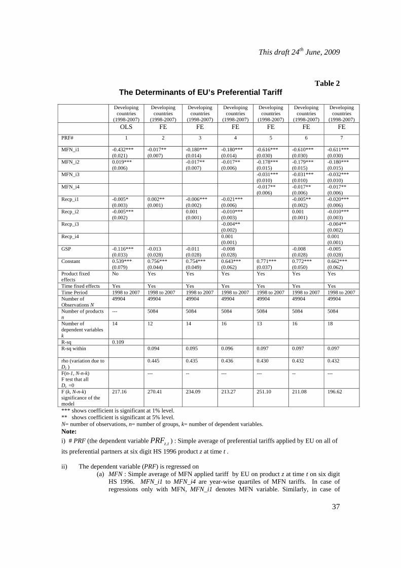
This draft 24th June, 2009
37
Table 2
The Determinants of EU’s Preferential Tariff
*** shows coefficient is significant at 1% level. ** shows coefficient is significant at 5% level. N= number of observations, n= number of groups, k= number of dependent variables. Note: i) # PRF (the dependent variable ,z tPRF ) : Simple average of preferential tariffs applied by EU on all of its preferential partners at six digit HS 1996 product z at time t . ii) The dependent variable (PRF) is regressed on
(a) MFN : Simple average of MFN applied tariff by EU on product z at time t on six digit HS 1996. MFN_i1 to MFN_i4 are year-wise quartiles of MFN tariffs. In case of regressions only with MFN, MFN_i1 denotes MFN variable. Similarly, in case of
Developing countries
(1998-2007)
Developing countries
(1998-2007)
Developing countries
(1998-2007)
Developing countries
(1998-2007)
Developing countries
(1998-2007)
Developing countries
(1998-2007)
Developing countries
(1998-2007) OLS FE FE FE FE FE FE PRF# 1 2 3 4 5 6 7
MFN_i1 -0.432*** (0.021)
-0.017** (0.007)
-0.180*** (0.014)
-0.180*** (0.014)
-0.616*** (0.030)
-0.610*** (0.030)
-0.611*** (0.030)
MFN_i2 0.019*** (0.006)
-0.017** (0.007)
-0.017** (0.006)
-0.178*** (0.015)
-0.179*** (0.015)
-0.180*** (0.015)
MFN_i3 -0.031*** (0.010)
-0.031*** (0.010)
-0.032*** (0.010)
MFN_i4 -0.017** (0.006)
-0.017** (0.006)
-0.017** (0.006)
Recp_i1 -0.005* (0.003)
0.002** (0.001)
-0.006*** (0.002)
-0.021*** (0.006)
-0.005** (0.002)
-0.020*** (0.006)
Recp_i2 -0.005*** (0.002)
0.001 (0.001)
-0.010*** (0.003)
0.001 (0.001)
-0.010*** (0.003)
Recp_i3 -0.004** (0.002)
-0.004** (0.002)
Recp_i4 0.001 (0.001)
0.001 (0.001)
GSP -0.116*** (0.033)
-0.013 (0.028)
-0.011 (0.028)
-0.008 (0.028)
-0.008 (0.028)
-0.005 (0.028)
Constant 0.539*** (0.079)
0.756*** (0.044)
0.754*** (0.049)
0.643*** (0.062)
0.771*** (0.037)
0.772*** (0.050)
0.662*** (0.062)
Product fixed effects
No Yes Yes Yes Yes Yes Yes
Time fixed effects Yes Yes Yes Yes Yes Yes Yes Time Period 1998 to 2007 1998 to 2007 1998 to 2007 1998 to 2007 1998 to 2007 1998 to 2007 1998 to 2007Number of Observations N
49904 49904 49904 49904 49904 49904 49904
Number of products n
--- 5084 5084 5084 5084 5084 5084
Number of dependent variables k
14 12 14 16 13 16 18
R-sq 0.109 R-sq within 0.094 0.095
0.096
0.097 0.097 0.097
rho (variation due to Dz )
0.445 0.435 0.436 0.430 0.432 0.432
F(n-1, N-n-k) F test that all Dz =0
--- -- --- --- -- ---
F (k, N-n-k) significance of the model
217.16 270.41 234.09 213.27 251.10 211.08 196.62
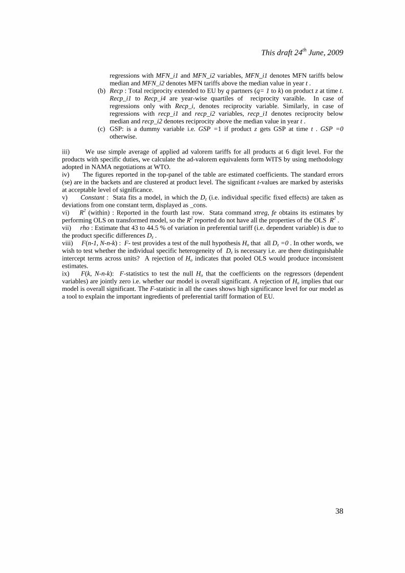
This draft 24th June, 2009
38
regressions with MFN_i1 and MFN_i2 variables, MFN_i1 denotes MFN tariffs below median and MFN_i2 denotes MFN tariffs above the median value in year t .
(b) Recp : Total reciprocity extended to EU by q partners (q= 1 to k) on product z at time t. Recp_i1 to Recp_i4 are year-wise quartiles of reciprocity varaible. In case of regressions only with Recp_i, denotes reciprocity variable. Similarly, in case of regressions with recp_i1 and recp_i2 variables, recp_i1 denotes reciprocity below median and recp_i2 denotes reciprocity above the median value in year t .
(c) GSP: is a dummy variable i.e. GSP =1 if product z gets GSP at time t . GSP =0 otherwise.
iii) We use simple average of applied ad valorem tariffs for all products at 6 digit level. For the products with specific duties, we calculate the ad-valorem equivalents form WITS by using methodology adopted in NAMA negotiations at WTO. iv) The figures reported in the top-panel of the table are estimated coefficients. The standard errors (se) are in the backets and are clustered at product level. The significant t-values are marked by asterisks at acceptable level of significance. v) Constant : Stata fits a model, in which the Dz (i.e. individual specific fixed effects) are taken as deviations from one constant term, displayed as _cons. vi) R2 (within) : Reported in the fourth last row. Stata command xtreg, fe obtains its estimates by performing OLS on transformed model, so the R2 reported do not have all the properties of the OLS R2 . vii) rho : Estimate that 43 to 44.5 % of variation in preferential tariff (i.e. dependent variable) is due to the product specific differences Dz . viii) F(n-1, N-n-k) : F- test provides a test of the null hypothesis Ho that all Dz =0 . In other words, we wish to test whether the individual specific heterogeneity of Dz is necessary i.e. are there distinguishable intercept terms across units? A rejection of Ho indicates that pooled OLS would produce inconsistent estimates. ix) F(k, N-n-k): F-statistics to test the null Ho that the coefficients on the regressors (dependent variables) are jointly zero i.e. whether our model is overall significant. A rejection of Ho implies that our model is overall significant. The F-statistic in all the cases shows high significance level for our model as a tool to explain the important ingredients of preferential tariff formation of EU.

This draft 24th June, 2009
39
Table3
The Determinants of EU’s Preferential Tariff
*** shows coefficient is significant at 1% level. ** shows coefficient is significant at 5% level. N= number of observations, n= number of groups, k= number of dependent variables.
All Partners (1995-2007)
All Partners (1995-2007)
All Partners (1995-2007)
All Partners (1995-2007)
Developing countries
(1998-2007)
Developing countries
(1998-2007)
Developing countries
(1998-2007) FE FE FE FE FE FE FE PRF# 1 2 3 4 5 6 7
MFN_af_i1 -2.562*** (0.417)
-2.497*** (0.411)
-2.506*** (0.412)
-2.527*** (0.414)
-0.828** (0.333)
-0.840** (0.335)
-0.845** (0.339)
MFN_af_i2 -0.212*** (0.065)
-0.200*** (0.064)
-0.200*** (0.064)
-0.201 *** (0.064)
-0.064*** (0.021)
-0.063*** (0.021)
-0.062*** (0.021)
MFN_af_i3 -0.066 (0.043)
-0.065 (0.043)
-0.064 (0.043)
-0.064 (0.043)
-0.049*** (0.016)
-0.048*** (0.016)
-0.047*** (0.016)
MFN_af_i4 0.040 (0.028)
0.040 (0.027)
0.040 (0.027)
0.040 (0.027)
-0.017*** (0.006)
-0.017*** (0.006)
-0.017*** (0.006)
MFN_na_i1 -1.064*** (0.091)
-1.018*** (0.086)
-1.007*** (0.085)
-1.000*** (0.085)
-0.494*** (0.034)
-0.486*** (0.034)
-0.484*** (0.034)
MFN_na_i2 -0.613*** (0.062)
-0.588*** (0.059)
-0.584*** (0.059)
-0.582*** (0.059)
-0.143*** (0.019)
-0.142*** (0.019)
-0.142*** (0.019)
MFN_na_i3 -0.232*** (0.032)
-0.221*** (0.031)
-0.220*** (0.031)
-0.221*** (0.031)
0.065*** (0.009)
0.064*** (0.009)
0.063*** (0.009)
MFN_na_i4 -0.090*** (0.023)
-0.082*** (0.022)
-0.081*** (0.022)
-0.080*** (0.022)
0.105*** (0.005)
0.105*** (0.005)
0.105*** (0.005)
Recp_i1 -0.014*** (0.004)
-0.044*** (0.010)
-0.006*** (0.002)
-0.018*** (0.006)
Recp_i2 -0.001 (0.002)
-0.026*** (0.005)
0.001 (0.001)
-0.010*** (0.003)
Recp_i3 -0.014*** (0.003)
-0.004** (0.002)
Recp_i4 -0.002 (0.002)
0.001 (0.001)
GSP -0.958*** (0.104)
-0.954*** (0.103)
-0.946*** (0.102)
-0.012 (0.028)
-0.007 (0.028)
-0.005 (0.027)
Constant 1.377*** (0.120)
1.891*** (0.162)
1.737*** (0.177)
1.433*** (0.170)
0.464*** (0.032)
0.451*** (0.044)
0.351 (0.054)
Product fixed effects
Yes Yes Yes Yes Yes Yes Yes
Time fixed effects Yes Yes Yes Yes Yes Yes Yes Time Period 1995 to 2007 1995 to 2007 1995 to 2007 1995 to 2007 1998 to 2007 1998 to 2007 1998 to 2007Number of Observations N
65148 65148 65148 65148 49904 49904 49904
Number of products n
5102 5102 5102 5102 5084 5084 5084
Number of dependent variables k
20 21 23 25 18 20 22
R-sq R-sq within 0.049 0.053 0.054 0.054 0.101 0.101 0.101 rho (variation due to Dz )
0.196 0.195 0.195 0.196 0.406 0.408 0.409
F(n-1, N-n-k) F test that all Dz =0
-- -- --- -- -- --- --
F (k, N-n-k) significance of the model
167.20 153.85 141.62 132.03 296.66 268.84 249.17

This draft 24th June, 2009
40
Note: i) # PRF (the dependent variable ,z tPRF ) : Simple average of preferential tariffs applied by EU on all of its preferential partners at six digit HS 1996 product z at time t . ii) The dependent variable (PRF) is regressed on
(a) MFN : Simple average of MFN applied tariff by EU on product z at time t on six digit HS 1996. MFN_af_i1 to MFN_af_i4 are year-wise quartiles of MFN tariffs on agricultural products. MFN_na_i1 to MFN_na_i4 are year-wise quartiles of MFN tariffs on industrial products.
(b) Recp : Total reciprocity extended to EU by q partners (q= 1 to k) on product z at time t Recp_i1 to Recp_i4 are year-wise quartiles of reciprocity variable.
(c) GSP: is a dummy variable i.e. GSP =1 if product z gets GSP at time t . GSP =0 otherwise.
iii) We use simple average of applied ad valorem tariffs for all products at 6 digit level. For the products with specific duties, we calculate the ad-valorem equivalents form WITS by using methodology adopted in NAMA negotiations at WTO. iv) The figures reported in the top-panel of the table are estimated coefficients. The standard errors (se) are in the backets and are clustered at product level. The significant t-values are marked by asterisks at acceptable level of significance. v) Constant : Stata fits a model, in which the Dz (i.e. individual specific fixed effects) are taken as deviations from one constant term, displayed as _cons. vi) R2 (within) : Reported in the fourth last row. Stata command xtreg, fe obtains its estimates by performing OLS on transformed model, so the R2 reported do not have all the properties of the OLS R2 . vii) rho : Estimate that percentage of variation in preferential tariff (i.e. dependent variable) that is due to the product specific differences Dz . viii) F(n-1, N-n-k) : F- test provides a test of the null hypothesis Ho that all Dz =0 . In other words, we wish to test whether the individual specific heterogeneity of Dz is necessary i.e. are there distinguishable intercept terms across units? A rejection of Ho indicates that pooled OLS would produce inconsistent estimates. ix) F(k, N-n-k): F-statistics to test the null Ho that the coefficients on the regressors (dependent variables) are jointly zero i.e. whether our model is overall significant. A rejection of Ho implies that our model is overall significant. The F-statistic in all the cases shows high significance level for our model as a tool to explain the important ingredients of preferential tariff formation of EU.


