Prelim Notes for Numerical Analysisweb.utk.edu/~wfeng1/doc/PrelimNum.pdf · Wenqiang Feng Prelim...

Prelim Notes for Numerical Analysis ∗

Wenqiang Feng †

Abstract

This note is intended to assist my prelim examination preparation. You can download and distributeit. Please be aware, however, that the note contains typos as well as incorrect or inaccurate solutions . Athere, I also would like to thank Liguo Wang for his help in some problems. This note is based on the Dr.Abner J. Salgado’s lecture note [4]. Some solutions are from Dr. Steven Wise’s lecture note [5].

∗Key words: UTK, PDE, Prelim exam, Numerical Analysis.†Department of Mathematics,University of Tennessee, Knoxville, TN, 37909, [email protected]

1

Contents

List of Figures 4

List of Tables 4

1 Preliminaries 51.1 Linear Algebra Preliminaries . . . . . . . . . . . . . . . . . . . . . . . . . . . . . . . . . . . . 5

1.1.1 Common Properties . . . . . . . . . . . . . . . . . . . . . . . . . . . . . . . . . . . . . 51.1.2 Similar and diagonalization . . . . . . . . . . . . . . . . . . . . . . . . . . . . . . . . 71.1.3 Eigenvalues and Eigenvectors . . . . . . . . . . . . . . . . . . . . . . . . . . . . . . . 71.1.4 Unitary matrices . . . . . . . . . . . . . . . . . . . . . . . . . . . . . . . . . . . . . . . 81.1.5 Hermitian matrices . . . . . . . . . . . . . . . . . . . . . . . . . . . . . . . . . . . . . 91.1.6 Positive definite matrices . . . . . . . . . . . . . . . . . . . . . . . . . . . . . . . . . . 111.1.7 Normal matrices . . . . . . . . . . . . . . . . . . . . . . . . . . . . . . . . . . . . . . . 111.1.8 Common Theorems . . . . . . . . . . . . . . . . . . . . . . . . . . . . . . . . . . . . . 12

1.2 Calculus Preliminaries . . . . . . . . . . . . . . . . . . . . . . . . . . . . . . . . . . . . . . . . 121.3 Preliminary Inequalities . . . . . . . . . . . . . . . . . . . . . . . . . . . . . . . . . . . . . . . 131.4 Norms’ Preliminaries . . . . . . . . . . . . . . . . . . . . . . . . . . . . . . . . . . . . . . . . . 27

1.4.1 Vector Norms . . . . . . . . . . . . . . . . . . . . . . . . . . . . . . . . . . . . . . . . 271.4.2 Matrix Norms . . . . . . . . . . . . . . . . . . . . . . . . . . . . . . . . . . . . . . . . 28

1.5 Problems . . . . . . . . . . . . . . . . . . . . . . . . . . . . . . . . . . . . . . . . . . . . . . . . 30

2 Direct Method 332.1 For squared or rectangular matrices A ∈ Cm,n,m ≥ n . . . . . . . . . . . . . . . . . . . . . . . 33

2.1.1 Singular Value Decomposition . . . . . . . . . . . . . . . . . . . . . . . . . . . . . . . 332.1.2 Gram-Schmidt orthogonalization . . . . . . . . . . . . . . . . . . . . . . . . . . . . . 342.1.3 QR Decomposition . . . . . . . . . . . . . . . . . . . . . . . . . . . . . . . . . . . . . 35

2.2 For squared matrices A ∈ Cn,n . . . . . . . . . . . . . . . . . . . . . . . . . . . . . . . . . . . . 362.2.1 Condition number . . . . . . . . . . . . . . . . . . . . . . . . . . . . . . . . . . . . . . 362.2.2 LU Decomposition . . . . . . . . . . . . . . . . . . . . . . . . . . . . . . . . . . . . . . 372.2.3 Cholesky Decomposition . . . . . . . . . . . . . . . . . . . . . . . . . . . . . . . . . . 382.2.4 The Relationship of the Existing Decomposition . . . . . . . . . . . . . . . . . . . . 392.2.5 Regular Splittings[3] . . . . . . . . . . . . . . . . . . . . . . . . . . . . . . . . . . . . 39

2.3 Problems . . . . . . . . . . . . . . . . . . . . . . . . . . . . . . . . . . . . . . . . . . . . . . . . 40

3 Iterative Method 433.1 Diagonal dominant . . . . . . . . . . . . . . . . . . . . . . . . . . . . . . . . . . . . . . . . . . 433.2 General Iterative Scheme . . . . . . . . . . . . . . . . . . . . . . . . . . . . . . . . . . . . . . 433.3 Stationary cases iterative method . . . . . . . . . . . . . . . . . . . . . . . . . . . . . . . . . . 45

3.3.1 Jacobi Method . . . . . . . . . . . . . . . . . . . . . . . . . . . . . . . . . . . . . . . . 453.3.2 Gauss-Seidel Method . . . . . . . . . . . . . . . . . . . . . . . . . . . . . . . . . . . . 463.3.3 Richardson Method . . . . . . . . . . . . . . . . . . . . . . . . . . . . . . . . . . . . . 483.3.4 Successive Over Relaxation (SOR) Method . . . . . . . . . . . . . . . . . . . . . . . . 50

3.4 Convergence in energy norm for steady cases . . . . . . . . . . . . . . . . . . . . . . . . . . . 523.5 Dynamic cases iterative method . . . . . . . . . . . . . . . . . . . . . . . . . . . . . . . . . . 53

3.5.1 Chebyshev iterative Method . . . . . . . . . . . . . . . . . . . . . . . . . . . . . . . . 533.5.2 Minimal residuals Method . . . . . . . . . . . . . . . . . . . . . . . . . . . . . . . . . 543.5.3 Minimal correction iterative method . . . . . . . . . . . . . . . . . . . . . . . . . . . 553.5.4 Steepest Descent Method . . . . . . . . . . . . . . . . . . . . . . . . . . . . . . . . . . 583.5.5 Conjugate Gradients Method . . . . . . . . . . . . . . . . . . . . . . . . . . . . . . . . 59

2

Wenqiang Feng Prelim Exam note for Numerical Analysis Page 3

3.5.6 Another look at Conjugate Gradients Method . . . . . . . . . . . . . . . . . . . . . . 593.6 Problems . . . . . . . . . . . . . . . . . . . . . . . . . . . . . . . . . . . . . . . . . . . . . . . . 61

4 Eigenvalue Problems 634.1 Schur algorithm . . . . . . . . . . . . . . . . . . . . . . . . . . . . . . . . . . . . . . . . . . . . 654.2 QR algorithm . . . . . . . . . . . . . . . . . . . . . . . . . . . . . . . . . . . . . . . . . . . . . 654.3 Power iteration algorithm . . . . . . . . . . . . . . . . . . . . . . . . . . . . . . . . . . . . . . 664.4 Inverse Power iteration algorithm . . . . . . . . . . . . . . . . . . . . . . . . . . . . . . . . . 684.5 Problems . . . . . . . . . . . . . . . . . . . . . . . . . . . . . . . . . . . . . . . . . . . . . . . . 68

5 Solution of Nonlinear problems 695.1 Bisection method . . . . . . . . . . . . . . . . . . . . . . . . . . . . . . . . . . . . . . . . . . . 695.2 Chord method . . . . . . . . . . . . . . . . . . . . . . . . . . . . . . . . . . . . . . . . . . . . . 695.3 Secant method . . . . . . . . . . . . . . . . . . . . . . . . . . . . . . . . . . . . . . . . . . . . 705.4 Newton’s method . . . . . . . . . . . . . . . . . . . . . . . . . . . . . . . . . . . . . . . . . . . 705.5 Newton’s method for system . . . . . . . . . . . . . . . . . . . . . . . . . . . . . . . . . . . . 725.6 Fixed point method . . . . . . . . . . . . . . . . . . . . . . . . . . . . . . . . . . . . . . . . . . 745.7 Problems . . . . . . . . . . . . . . . . . . . . . . . . . . . . . . . . . . . . . . . . . . . . . . . . 74

6 Euler Method 796.1 Euler’s method . . . . . . . . . . . . . . . . . . . . . . . . . . . . . . . . . . . . . . . . . . . . 796.2 Trapezoidal Method . . . . . . . . . . . . . . . . . . . . . . . . . . . . . . . . . . . . . . . . . 826.3 Theta Method . . . . . . . . . . . . . . . . . . . . . . . . . . . . . . . . . . . . . . . . . . . . . 846.4 Midpoint Rule Method . . . . . . . . . . . . . . . . . . . . . . . . . . . . . . . . . . . . . . . . 856.5 Problems . . . . . . . . . . . . . . . . . . . . . . . . . . . . . . . . . . . . . . . . . . . . . . . . 87

7 Multistep Methond 887.1 The Adams Method . . . . . . . . . . . . . . . . . . . . . . . . . . . . . . . . . . . . . . . . . . 887.2 The Order and Convergence of Multistep Methods . . . . . . . . . . . . . . . . . . . . . . . . 887.3 Method of A-stable verification for Multistep Methods . . . . . . . . . . . . . . . . . . . . . 897.4 Problems . . . . . . . . . . . . . . . . . . . . . . . . . . . . . . . . . . . . . . . . . . . . . . . . 89

8 Runge-Kutta Methods 958.1 Quadrature Formulas . . . . . . . . . . . . . . . . . . . . . . . . . . . . . . . . . . . . . . . . 958.2 Explicit Runge-Kutta Formulas . . . . . . . . . . . . . . . . . . . . . . . . . . . . . . . . . . . 958.3 Implicit Runge-Kutta Formulas . . . . . . . . . . . . . . . . . . . . . . . . . . . . . . . . . . . 968.4 Method of A-stable verification for Runge-Kutta Method . . . . . . . . . . . . . . . . . . . . 968.5 Problems . . . . . . . . . . . . . . . . . . . . . . . . . . . . . . . . . . . . . . . . . . . . . . . . 96

9 Finite Difference Method 979.1 Problems . . . . . . . . . . . . . . . . . . . . . . . . . . . . . . . . . . . . . . . . . . . . . . . . 100

10 Finite Element Method 10610.1 Finite element methods for 1D elliptic problems . . . . . . . . . . . . . . . . . . . . . . . . . 10810.2 Problems . . . . . . . . . . . . . . . . . . . . . . . . . . . . . . . . . . . . . . . . . . . . . . . . 111

References 113

Appendices 114

Appendix 114

Page 3 of 236

A Numerical Mathematics Preliminary Examination Sample Question, Summer, 2013 114A.1 Numerical Linear Algebra . . . . . . . . . . . . . . . . . . . . . . . . . . . . . . . . . . . . . . 114A.2 Numerical Solutions of Nonlinear Equations . . . . . . . . . . . . . . . . . . . . . . . . . . . 130A.3 Numerical Solutions of ODEs . . . . . . . . . . . . . . . . . . . . . . . . . . . . . . . . . . . . 134A.4 Numerical Solutions of PDEs . . . . . . . . . . . . . . . . . . . . . . . . . . . . . . . . . . . . 135A.5 Supplemental Problems . . . . . . . . . . . . . . . . . . . . . . . . . . . . . . . . . . . . . . . 147

B Numerical Mathematics Preliminary Examination 148B.1 Numerical Mathematics Preliminary Examination Jan. 2011 . . . . . . . . . . . . . . . . . . 148B.2 Numerical Mathematics Preliminary Examination Aug. 2010 . . . . . . . . . . . . . . . . . . 155B.3 Numerical Mathematics Preliminary Examination Jan. 2009 . . . . . . . . . . . . . . . . . . 160B.4 Numerical Mathematics Preliminary Examination Jan. 2008 . . . . . . . . . . . . . . . . . . 160

C Project 1 MATH571 161

D Project 2 MATH571 177

E Midterm examination 572 189

F Project 1 MATH572 196

G Project 2 MATH572 214

List of Figures

1 The curve of ρ(TRC) as a function of ω . . . . . . . . . . . . . . . . . . . . . . . . . . . . . . . 50

2 The curve of ρ(TR) as a function of w . . . . . . . . . . . . . . . . . . . . . . . . . . . . . . . 61

3 One dimension’s uniform partition . . . . . . . . . . . . . . . . . . . . . . . . . . . . . . . . 98

A1 One dimension’s uniform partition . . . . . . . . . . . . . . . . . . . . . . . . . . . . . . . . 139

B2 The curve of ρ(TR) as a function of w . . . . . . . . . . . . . . . . . . . . . . . . . . . . . . . 148

List of Tables

4


1 Preliminaries

1.1 Linear Algebra Preliminaries

1.1.1 Common Properties

Properties 1.1. (Structure of Matrices) Let A= [Aij ] be a square or rectangular matrix, A is called

• diagonal : if aij = 0, ∀i , j,

• upper triangular : if aij = 0, ∀i > j,

• upper Hessenberg : if aij = 0, ∀i > j + 1,

• block diagonal :A= diag(A11,A22, · · · ,Ann),

• tridiagonal : if aij = 0, ∀|i − j | > 1,

• lower triangular : if aij = 0, ∀i < j,

• lower Hessenberg : if aij = 0, ∀j > i+ 1,

• block diagonal :A= diag(Ai,i−1,Aii , · · · ,Ai,i+1).

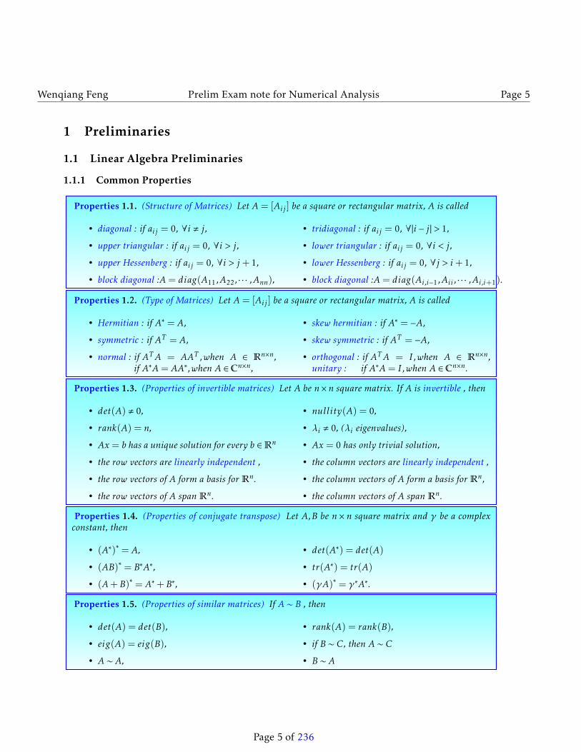
Properties 1.2. (Type of Matrices) Let A= [Aij ] be a square or rectangular matrix, A is called

• Hermitian : if A∗ = A,

• symmetric : if AT = A,

• normal : if ATA = AAT ,when A ∈ Rn×n,if A∗A= AA∗,when A ∈ Cn×n,

• skew hermitian : if A∗ = −A,

• skew symmetric : if AT = −A,

• orthogonal : if ATA = I ,when A ∈ Rn×n,unitary : if A∗A= I ,when A ∈ Cn×n.

Properties 1.3. (Properties of invertible matrices) Let A be n×n square matrix. If A is invertible , then

• det(A) , 0,

• rank(A) = n,

• Ax = b has a unique solution for every b ∈Rn

• the row vectors are linearly independent ,

• the row vectors of A form a basis for Rn.

• the row vectors of A span Rn.

• nullity(A) = 0,

• λi , 0, (λi eigenvalues),

• Ax = 0 has only trivial solution,

• the column vectors are linearly independent ,

• the column vectors of A form a basis for Rn,

• the column vectors of A span Rn.

Properties 1.4. (Properties of conjugate transpose) Let A,B be n × n square matrix and γ be a complexconstant, then

• (A∗)∗ = A,

• (AB)∗ = B∗A∗,

• (A+B)∗ = A∗+B∗,

• det(A∗) = det(A)

• tr(A∗) = tr(A)

• (γA)∗ = γ∗A∗.

Properties 1.5. (Properties of similar matrices) If A ∼ B , then

• det(A) = det(B),

• eig(A) = eig(B),

• A ∼ A,

• rank(A) = rank(B),

• if B ∼ C, then A ∼ C

• B ∼ A

Page 5 of 236


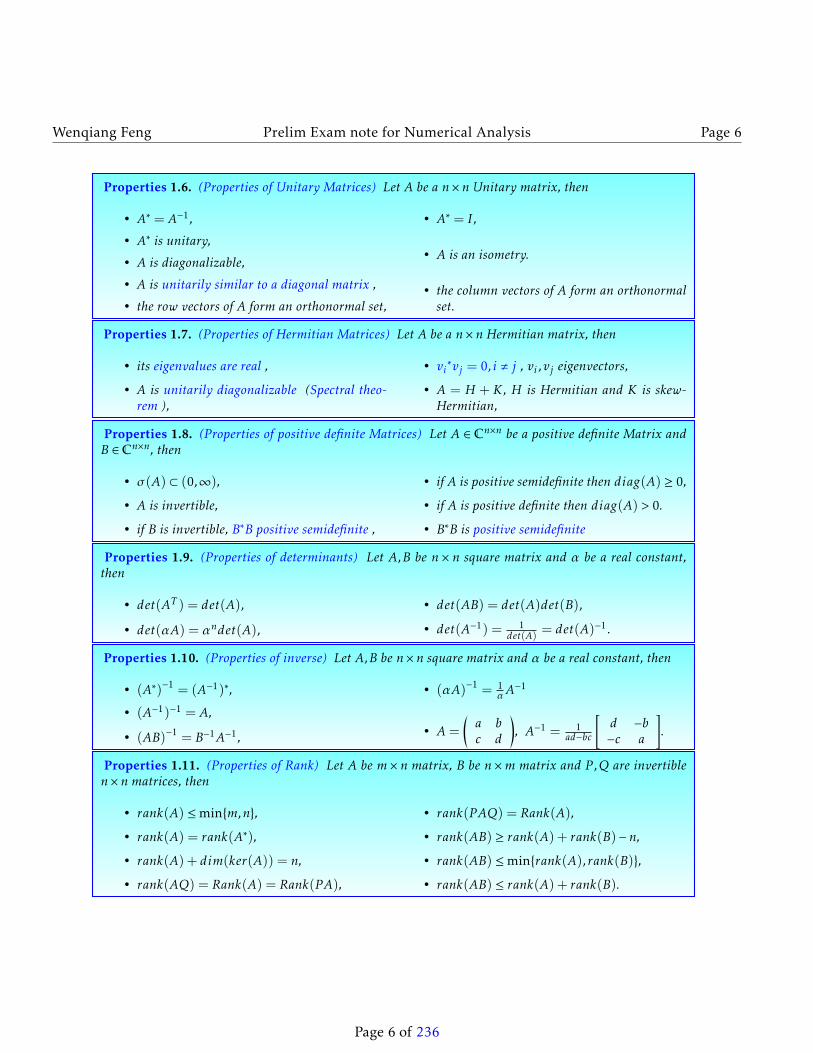
Properties 1.6. (Properties of Unitary Matrices) Let A be a n×n Unitary matrix, then

• A∗ = A−1,

• A∗ is unitary,

• A is diagonalizable,

• A is unitarily similar to a diagonal matrix ,

• the row vectors of A form an orthonormal set,

• A∗ = I ,

• A is an isometry.

• the column vectors of A form an orthonormalset.

Properties 1.7. (Properties of Hermitian Matrices) Let A be a n×n Hermitian matrix, then

• its eigenvalues are real ,

• A is unitarily diagonalizable (Spectral theo-rem ),

• vi∗vj = 0, i , j , vi ,vj eigenvectors,

• A = H + K , H is Hermitian and K is skew-Hermitian,

Properties 1.8. (Properties of positive definite Matrices) Let A ∈ Cn×n be a positive definite Matrix andB ∈ Cn×n, then

• σ (A) ⊂ (0,∞),

• A is invertible,

• if B is invertible, B∗B positive semidefinite ,

• if A is positive semidefinite then diag(A) ≥ 0,

• if A is positive definite then diag(A) > 0.

• B∗B is positive semidefinite

Properties 1.9. (Properties of determinants) Let A,B be n × n square matrix and α be a real constant,then

• det(AT ) = det(A),

• det(αA) = αndet(A),

• det(AB) = det(A)det(B),

• det(A−1) = 1det(A)

= det(A)−1.

Properties 1.10. (Properties of inverse) Let A,B be n×n square matrix and α be a real constant, then

• (A∗)−1 = (A−1)∗,

• (A−1)−1 = A,

• (AB)−1 = B−1A−1,

• (αA)−1 = 1αA−1

• A=

(a bc d

), A−1 = 1

ad−bc

[d −b−c a

].

Properties 1.11. (Properties of Rank) Let A be m × n matrix, B be n ×m matrix and P ,Q are invertiblen×n matrices, then

• rank(A) ≤minm,n,

• rank(A) = rank(A∗),

• rank(A) + dim(ker(A)) = n,

• rank(AQ) = Rank(A) = Rank(PA),

• rank(PAQ) = Rank(A),

• rank(AB) ≥ rank(A) + rank(B)−n,

• rank(AB) ≤minrank(A),rank(B),

• rank(AB) ≤ rank(A) + rank(B).

Page 6 of 236


1.1.2 Similar and diagonalization

Theorem 1.1. (Similar) A is said to be similar to B, if there is a nonsingular matrix X, such that

A= XBX−1, (A ∼ B).

Theorem 1.2. (Diagonalizablea) A matrix is diagonalizable , if and only if there exist a nonsingularmatrix X and a diagonal matrix D such that A= XDX−1.

aBeing diagonalizable has nothing to do with being invertible.

Theorem 1.3. (Diagonalizable) A matrix is diagonalizable , if and only if all its eigenvalues are semisimple.

Theorem 1.4. (Diagonalizable) Suppose dim(A) = n. A is said to be diagonalizable , if and only if A hasn linearly independent eigenvectors .

Corollary 1.1. (Sample question #2, summer, 2013 ) Suppose dim(A) = n. IfA has n distinct eigenvalues, then A is diagonalizable .

Proof. (Sketch) Suppose n= 2, and let λ1,λ2 be distinct eigenvalues of A with corresponding eigenvectorsv1,v2. Now, we will use contradiction to show v1,v2 are lineally independent. Suppose v1,v2 are lineallydependent, then

c1v1 + c2v2 = 0, (1)

with c1,c2 are not both 0. Multiplying A on both sides of (210), then

c1Av1 + c2Av2 = c1λ1v1 + c2λ2v2 = 0. (2)

Multiplying λ1 on both sides of (210), then

c1λ1v1 + c2λ1v2 = 0. (3)

Subtracting (212) form (211), then

c2(λ2 −λ1)v2 = 0. (4)

Since λ1 , λ2 and v2 , 0, then c2 = 0. Similarly, we can get c1 = 0. Hence, we get the contradiction.A similar argument gives the result for n. Then we get A has n linearly independent eigenvectors .

Theorem 1.5. (Diagonalizable) Every Hermitian matrix is diagonalizable , In particular, every realsymmetric matrix is diagonalizable.

1.1.3 Eigenvalues and Eigenvectors

Theorem 1.6. if λ is an eigenvalue of A, then λ is an eigenvalue of A∗.

Theorem 1.7. The eigenvalues of a triangular matrix are the entries on its main diagonal.

Page 7 of 236


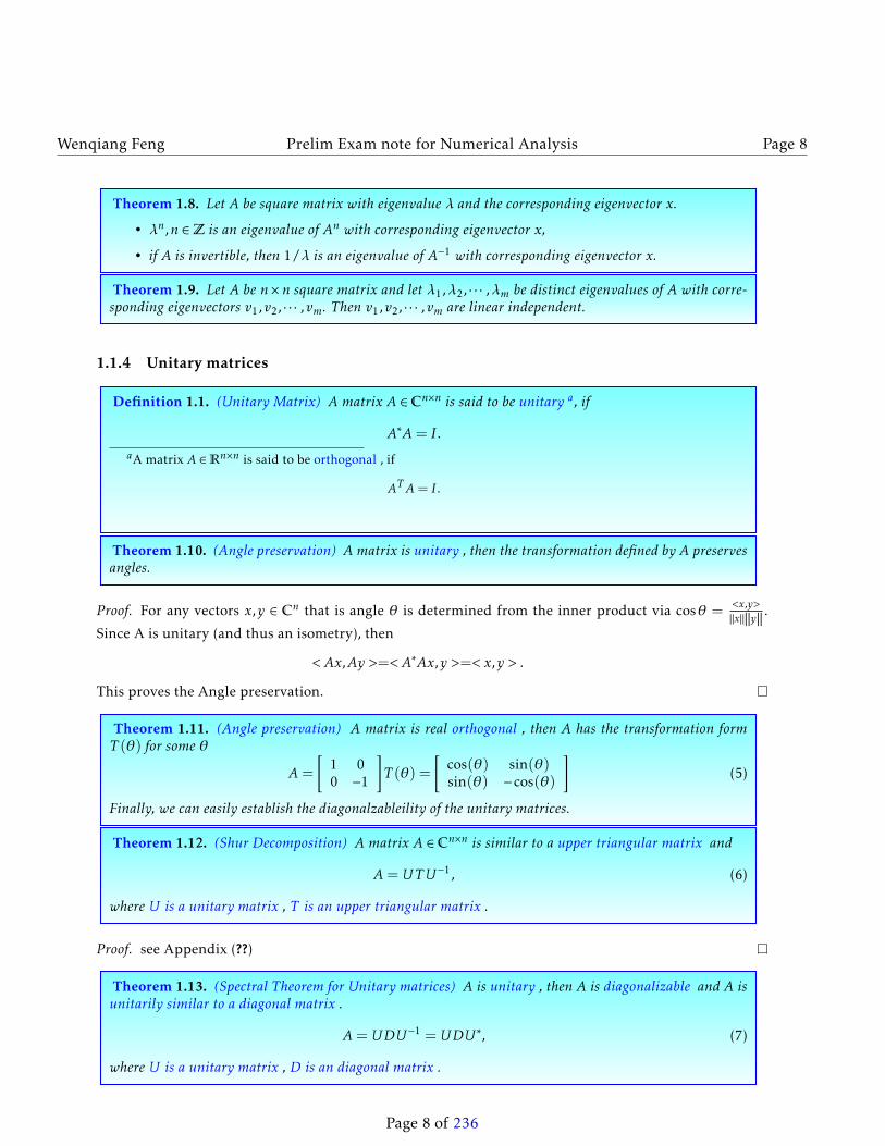
Theorem 1.8. Let A be square matrix with eigenvalue λ and the corresponding eigenvector x.

• λn,n ∈Z is an eigenvalue of An with corresponding eigenvector x,

• if A is invertible, then 1/λ is an eigenvalue of A−1 with corresponding eigenvector x.

Theorem 1.9. Let A be n×n square matrix and let λ1,λ2, · · · ,λm be distinct eigenvalues of A with corre-sponding eigenvectors v1,v2, · · · ,vm. Then v1,v2, · · · ,vm are linear independent.

1.1.4 Unitary matrices

Definition 1.1. (Unitary Matrix) A matrix A ∈ Cn×n is said to be unitary a, if

A∗A= I .aA matrix A ∈Rn×n is said to be orthogonal , if

ATA= I .

Theorem 1.10. (Angle preservation) A matrix is unitary , then the transformation defined by A preservesangles.

Proof. For any vectors x,y ∈ Cn that is angle θ is determined from the inner product via cosθ =<x,y>‖x‖‖y‖ .

Since A is unitary (and thus an isometry), then

< Ax,Ay >=< A∗Ax,y >=< x,y > .

This proves the Angle preservation.

Theorem 1.11. (Angle preservation) A matrix is real orthogonal , then A has the transformation formT (θ) for some θ

A=

[1 00 −1

]T (θ) =

[cos(θ) sin(θ)sin(θ) −cos(θ)

](5)

Finally, we can easily establish the diagonalzableility of the unitary matrices.

Theorem 1.12. (Shur Decomposition) A matrix A ∈ Cn×n is similar to a upper triangular matrix and

A= UTU−1, (6)

where U is a unitary matrix , T is an upper triangular matrix .

Proof. see Appendix (??)

Theorem 1.13. (Spectral Theorem for Unitary matrices) A is unitary , then A is diagonalizable and A isunitarily similar to a diagonal matrix .

A= UDU−1 = UDU ∗, (7)

where U is a unitary matrix , D is an diagonal matrix .

Page 8 of 236


Proof. Result follows from 1.12.

Theorem 1.14. (Spectral representiation) A is unitary , then

1. A has a set of n orthogonal eigenvectors,

2. let v1,v2, · · · ,vn be the eigenvalues w.r.t the corresponding orthogonal eigenvectors λ1,λ2, · · · ,λn.The A has the representation as the sum of rank one matrices given by

A=n∑i=1

λivivTi . (8)

Note: this representation is often called the Spectral Representation or Spectral Decomposition of A.

Proof. see Appendix (??)

1.1.5 Hermitian matrices

Definition 1.2. (Hermitian Matrix) A matrix is Hermitian , if

A∗ = A.

Definition 1.3. Let A be Hermitian , then the spectral of A, σ (A), is real.

Proof. Let λ ∈ σ (A) with corresponding eigenvector v. Then

< Av,v > = < λv,v >= λ < v,v > (9)

< Av,v > = < v,A∗v >=< v, λv >= λ < v,v > . (10)

Since < v,v >, 0,therefore λ= λ. Hence λ is real.

Definition 1.4. Let A be Hermitian , then the different eigenvector are orthogonal i.e.

< vi ,vj >= 0, i , j. (11)

Proof. Let λ1,λ2 be the arbitrary two different eigenvalues with corresponding eigenvector v1,v2. Then

< Av1,v2 > = < λ1v1,v2 >= λ1 < v1,v2 > (12)

< Av1,v2 > = < v1,A∗v2 >=< v1,Av2 >=< v,λ2v2 >= λ2 < v1,v2 > . (13)

Since λ1 , λ2,therefore < v1,v2 >= 0.

Theorem 1.15. (Spectral Theorem for Hermitian matrices) A is Hermitian , then A is unitary diagonal-izable .

A= UDU−1 = UDU ∗, (14)

where U is a unitary matrix , D is an diagonal matrix .

Theorem 1.16. If A,B are unitarily similar , then A is Hermitian if and only if B is Hermitian .

Page 9 of 236


Proof. Since A,B are unitarily similar , then A= UBU−1, where U is a unitary matrix . And

A∗ = U−1∗B∗U ∗ = U ∗−1B∗U ∗ = UB∗U−1,

since U is a unitary matrix. Therefore

UBU−1 = A= A∗ = UB∗U−1.

Hence, B= B∗.

Theorem 1.17. If A= A∗, then ρ(A) = ‖A‖2.

Proof. Since A is self-adjoint, there an orthonormal basis of eigenvector x ∈ Cn, s.t.

x = α1e1 +α2e2 + · · ·+αnen.

Moreover, Aei = λiei , ‖ei‖= 1 and (ei ,ej) = 0 when i . j,(ej ,ej) = 1. So,

‖x‖2`2 =n∑i=1

|αi |2,

since,

(x,x) = (n∑i=1

αiei ,n∑j=1

αjej)

=n∑i=1

n∑j=1

αi αjeiej

=n∑i=1

|αi |2.

Since, Ax = A(α1e1 +α2e2 + · · ·+αnen) = α1λ1e1 +α2λ2e2 + · · ·+αnλnen, then

‖Ax‖2`2 =n∑i=1

|λiαi |2 =n∑i=1

|λi |2|αi |2 ≤max|λi |2n∑i=1

|αi |2.

Therefore,

‖Ax‖`2 ≤ ρ(A)‖x‖`2 ,

i.e.

‖A‖2 = supx∈Cn

‖Ax‖`2

‖x‖`2≤ ρ(A).

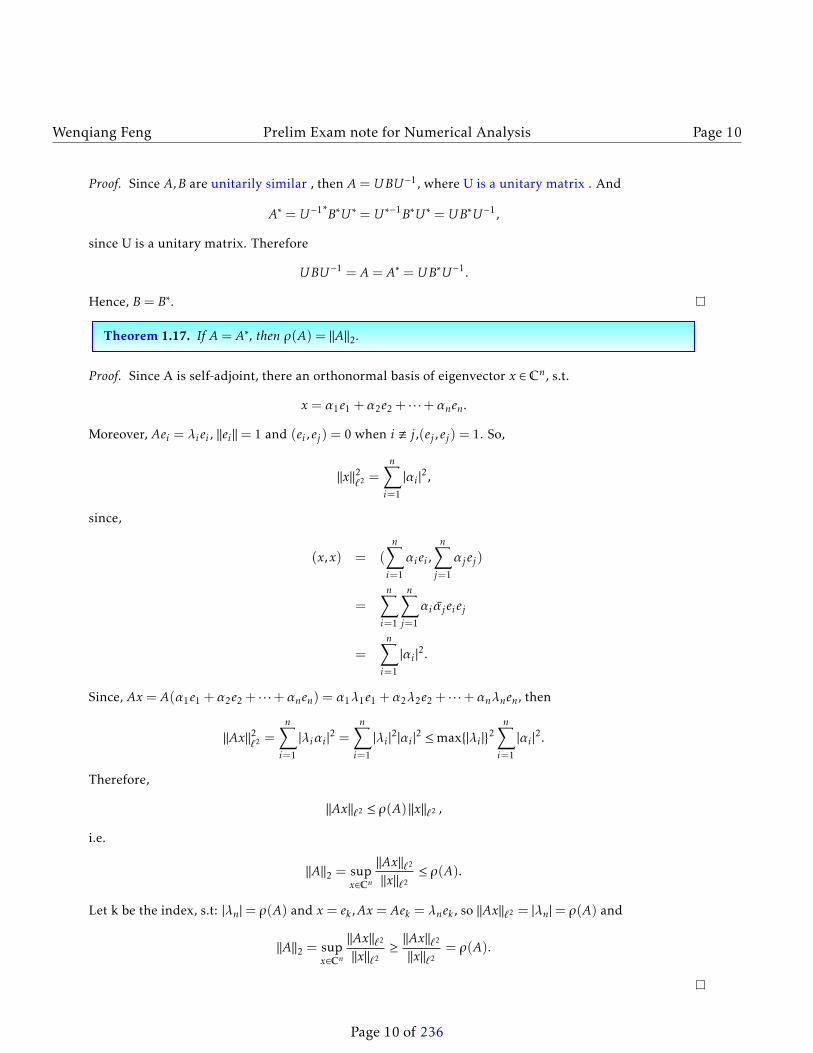
Let k be the index, s.t: |λn|= ρ(A) and x = ek ,Ax = Aek = λnek , so ‖Ax‖`2 = |λn|= ρ(A) and

‖A‖2 = supx∈Cn

‖Ax‖`2

‖x‖`2≥ ‖

Ax‖`2

‖x‖`2= ρ(A).

Page 10 of 236


1.1.6 Positive definite matrices

Definition 1.5. (Positive Definite Matrix)

1. A symmetric real matrix A ∈Rn×n is said to be Positive Definite , if

xTAx > 0, ∀x , 0.

2. A Hermitian matrix A ∈ Cn×n is said to be Positive Definite , if

x∗Ax > 0, ∀x , 0.

Theorem 1.18. Let A,B ∈ Cn×n. Then

1. if A is positive definite, then σA ⊂ (0,∞),

2. if A is positive definite, then A is invertible,

3. B∗B is positive semidefinite,

4. if B is invertible, then B∗B is positive definite.

5. if B is positive definite, then diag(B) is nonnegative,

6. if diag(B) strictly positive, thenif B is positive definite.

Problem 1.1. (Sample question #1, summer, 2013 ) Suppose A ∈ Cn×n is hermitian and σ (A) ⊂ (0,∞).Prove A is Hermitian Positive Defined (HPD).

Proof. Since, A is Hermitian, then is Unitary diagonalizable. i.e. A= UDU−1 = UDU ∗, then

x∗Ax = x∗UDU−1x = x∗UDU ∗x = (U ∗x)∗D(U ∗x). (15)

Moreover, since σ (A) ⊂ (0,∞) then x∗Dx > 0 for any nonzero x. Hence

x∗Ax = (U ∗x)∗D(U ∗x) = x∗Dx > 0, for any nonzero x. (16)

1.1.7 Normal matrices

Definition 1.6. (Normal Matrix) A matrix is called normal , if

A∗A= AA∗.

Corollary 1.2. Unitary matrix and Hermitian matrix are normal matrices.

Theorem 1.19. A ∈ Cn×n is normal if and only if every matrix unitarily equivalent to A is normal.

Theorem 1.20. A ∈ Cn×n is normal if and only if every matrix unitarily equivalent to A is normal.

Proof. Suppose A is normal and B = U ∗AU , where U is unitary. Then B∗B = U ∗A∗UU ∗AU = U ∗A∗AU =U ∗AA∗U = U ∗AUU ∗A∗U = BB∗, so B is normal. Conversely, If B is normal, it is easy to get that U ∗A∗AU =U ∗AA∗U , then A∗A= AA∗

Page 11 of 236


Theorem 1.21. (Spectral theorem for normal matrices) If A ∈ Cn×n has eigenvalues λ1, · · · ,λn, countedaccording to multiplicity, the following statements are equivalent.

1. A is normal,

2. A is unitarily diagonalizable,

3.∑ni=1

∑nj=1 |aij |2 =

∑ni=1 |λi |2,

4. There is an orthonormal set of n eigenvectors of A.

1.1.8 Common Theorems

Definition 1.7. (Orthogonal Complement) Suppose S ⊂Rn is a subspace. The (Orthogonal Complement)of S is defined as

S⊥ =y ∈Rn | yT x = 0,∀x ∈ S

Theorem 1.22. Suppose A ∈Rn×n. Then

1. R(A)⊥=N (AT ),

2. R(AT )⊥=N (A).

Proof. 1. For any y ∈ R(A)⊥, then yT y = 0,∀y ∈ R(A). And ∀y ∈ R(A), there exists x, such that Ax = y.Then

yTAx = (AT y)T x = 0.

Since, x is arbitrary, so it must be AT y = 0. Hence

R(A)⊥ ⊂N (AT )

Conversely, suppose y ∈ N (AT ), then AT y = 0 and hence (AT y)T x = yTAx = 0 for any x ∈ Rn. So,y ∈ R(AT )⊥. Therefore

N (AT ) ⊂R(A)⊥

R(A)⊥=N (AT ),

2. Similarly, we can prove R(AT )⊥=N (A),

1.2 Calculus Preliminaries

Definition 1.8. (Taylor formula for one variable) Let f (x) to be n-th differentiable at x0, then there existsa neighborhood B(x0,ε), ∀x ∈ B(x0,ε), s.t.

f (x) = f (x0) + f′(x0)(x − x0) +

f ′′(x0)

2!(x − x0)

2 + · · ·+f (n)(x0)

n!(x − x0)

n+O((x − x0)n+1)

= f (x0) + f′(x0)∆x+

f ′′(x0)

2!∆x2 + · · ·+

f (n)(x0)

n!∆xn+O(∆xn+1). (17)

Page 12 of 236


Definition 1.9. (Taylor formula for two variables) Let f (x,y) ∈ Ck+1(B((x0,y0),ε)), then ∀(x0 +∆x,y0 +∆y) ∈ B((x0,y0),ε)),

f (x0 +∆x,y0 +∆y) = f (x0,y0) +

(∆x

∂∂x

+∆y∂∂y

)f (x0,y0)

+12!

(∆x

∂∂x

+∆y∂∂y

)2

f (x0,y0) + · · · (18)

+1k!

(∆x

∂∂x

+∆y∂∂y

)kf (x0,y0) +Rk

where

Rk =1

(k+ 1)!

(∆x

∂∂x

+∆y∂∂y

)k+1

f (x0 +θ∆x,y0 +θ∆y), θ ∈ (0,1).

Definition 1.10. (Commonly used taylor series)

11− x

=∞∑n=0

xn = 1+ x+ x2 + x3 + x4 + · · · , x ∈ (−1,1), (19)

ex =∞∑n=0

xn

n!= 1+ x+

x2

2!+x3

3!+x4

4!+ · · · , x ∈R, (20)

sin(x) =∞∑n=0

(−1)nx2n+1

(2n+ 1)!= x − x

3

3!+x5

5!− x

7

7!+x9

9!− · · · , x ∈R, (21)

cos(x) =∞∑n=0

(−1)nx2n

(2n)!= 1− x

2

2!+x4

4!− x

6

6!+x8

8!− · · · , x ∈R, (22)

ln(1+ x) =∞∑n=0

(−1)nxn+1

n+ 1= x − x

2

2+x3

3− x

4

4+ · · · , x ∈ (−1,1). (23)

1.3 Preliminary Inequalities

Definition 1.11. (Cauchy’s Inequality)

ab ≤ a2

2+b2

2, for all a,b ∈R. (24)

Proof. Since (a− b)2 = a2 − 2ab+ b2 ≥ 0, therefore ab ≤ a2

2 + b2

2 , for all a,b ∈R.

Definition 1.12. (Cauchy’s Inequality with ε)

ab ≤ εa2 +b2

4ε, for all a,b > 0 , ε > 0. (25)

Proof. Using Cauchy’s Inequality with√

2εa, 1√2εb in place of a,b, we can get the result.

Page 13 of 236


Definition 1.13. (Young’s Inequality) Let 1 < p,q <∞, 1p +

1q = 1. Then

ab ≤ ap

p+bq

qfor all a,b > 0 . (26)

Proof. Firstly, we introduce an auxiliary function

f (t) =tp

p+

1q− t.

We know that the minimum value is at t = 1, since f ′(t) = tp−1 = 0 at t = 1. Now, we setting t = ab−q/p,we get

0 ≤ f (ab−q/p) =(ab−q/p)p

p+

1q− ab−q/p

=apb−q

p+

1q− ab−q/p.

So,

ab−q/p ≤ apb−q

p+

1q

.

Multiplying bq on both side of the above equation yields

abq−q/p ≤ ap

p+bq

q.

Since, 1p +

1q = 1, so pq = p+ q and q − q/p = 1. Hence

ab ≤ ap

p+bq

qfor all a,b > 0 .

Definition 1.14. (Young’s Inequality with ε)

ab ≤ εap +C(ε)bq, for all a,b > 0 , ε > 0, (27)

Where, C(ε) = (εp)−p/qq−1.

Proof. Using Young’s Inequality with (εp)1/pa,(

1εp

)1/pb in place of a,b, we can get the result.

Definition 1.15. (Hölder’s Inequality) Let 1 < p,q < ∞, 1p +

1q = 1. If u ∈ Lp(U ),v ∈ Lq(U ), then we

have uv ∈ L1(U ) and∫U|uv|dx ≤

(∫U|u|pdx

)1/p (∫U|v|qdx

)1/q

= ‖u‖Lp(U ) ‖v‖Lq(U ) . (28)

Page 14 of 236


Proof. Suppose∫U|u|pdx , 0 and

∫U|v|qdx , 0. Otherwise, if

∫U|u|pdx = 0, then u ≡ 0 a.e. and the Hölder’s

Inequality is trivial. We can use the same argument for v. Now, we define f ,g as following

f =|u|‖u‖Lp

,g =|v|‖v‖Lq

. (29)

Now applying Young’s inequality for f g, we have

f g =|u|‖u‖Lp

|v|‖v‖Lq

≤ 1p|u|p

‖u‖pLp+

1q|u|q

‖u‖qLq. (30)

Integrating it on U with respect to x, we obtain∫U

|u|‖u‖Lp

|v|‖v‖Lq

dx ≤∫U

1p|u|p

‖u‖pLp+

1q|u|q

‖u‖qLq

dx=

1p

∫U|u|pdx

‖u‖pLp+

1q

∫U|v|pdx

‖v‖qLq(31)

=1p+

1q= 1.

(31) implies that ∫U|u||v|dx ≤ ‖u‖Lp ‖v‖Lq . (32)

Hence ∫U|uv|dx ≤

∫U|u||v|dx ≤ ‖u‖Lp ‖v‖Lq . (33)

Corollary 1.3. (Hölder’s Inequality) Suppose that u ∈ L1(U ),v ∈ L∞(U ), then we have uv ∈ L1(U ) and∫U|uv|dx ≤ ‖u‖L1(U ) ‖v‖L∞(U ) . (34)

Proof. Since u ∈ L1(U ),v ∈ L∞(U ), so |uv| <∞ and∫U|uv|dx <∞. (35)

So uv ∈ L1(U ). ∫U|uv|dx ≤

∫U|u||v|dx ≤ ‖v‖L∞(U )

∫U|u|dx = ‖u‖L1(U ) ‖v‖L∞(U ) . (36)

Definition 1.16. (General Hölder’s Inequality) Let 1 < p1, · · · ,pn <∞, 1p1

+ · · ·+ 1pn

= 1r . If uk ∈ Lpk (U ),

then we have Πnk=1ui ∈ L

r(U ) and∫U|u1 · · ·un|rdx ≤Πn

k=1 ‖ui‖rLpk (U ). (37)

Page 15 of 236


Proof. We will use induction to prove General Hölder’s Inequality.

1. For k = 2, we have

1r=

1p1

+1p2

,

so r <min(p1,p2), Lp1 ⊂ Lr and Lp2 ⊂ Lr . Since u1 ∈ Lp1 and u2 ∈ Lp2 , so |u1u2| <∞ and∫U|u1u2|rdx <

∞. Therefore, u1u2 ∈ Lr(U ).

1 =1

p1/r+

1p2/r

.

Then applying Hölder’s inequality for |u1u2|r , we have∫U|u1u2|rdx

≤(∫

U(|u1|r)

p1r dx

) rp1

(∫U(|u2|r)

p2r dx

) rp2

=

(∫U|u1|p1dx

) rp1

(∫U|u2|p2dx

) rp2

≤ ‖u1‖rLp1 (U ) ‖u2‖rLp2 (U ) .

2. Induction assumption: Assume the inequality holds for k = n− 1, i.e. Πnk=1ui ∈ L

r(U ) and∫U|u1 · · ·un−1|rdx ≤Πn−1

k=1 ‖ui‖rLpk (U ).

3. Induction result: for k = n, we have

1p1

+ · · ·+ 1pn

=1r

.

so r < min(p1,p2, · · · ,pn) and Lpk ⊂ Lr . Since uk ∈ Lpk , so Πnk=1|ui | ∈ L

r(U ) <∞ and∫U|u1 · · ·un|rdx <

∞. Therefore, Πnk=1ui ∈ L

r(U ). let

1p1

+ · · ·+ 1pn−1

=1p

.

so

1p+

1pn

=1r

.

From the Hölder’s inequality for n= 2 and the induction assumption, we have∫U|u1 · · ·un|rdx ≤

(∫U|u1 · · ·un−1|pdx

) rp(∫

U|un|pndx

) rpn

≤ ‖u1‖rLp(U ) ‖u2‖rLpn (U ) =Πnk=1 ‖ui‖

rLpk (U ).

Page 16 of 236


Corollary 1.4. (General Hölder’s Inequality) Let 1 < p1, · · · ,pn <∞, 1p1

+ · · ·+ 1pn

= 1. If uk ∈ Lpk (U ),

then we have Πnk=1ui ∈ L

1(U ) and∫U|u1 · · ·un|dx ≤Πn

k=1 ‖ui‖Lpk (U ). (38)

for k = 1,2, · · · ,n− 1.

Proof. Take r = 1 in last General Hölder’s Inequality.

Definition 1.17. (Discrete Hölder’s Inequality) Let 1 < p,q <∞, 1p +

1q = 1. Then for all ak ,bk ∈Rn,∣∣∣∣∣∣∣

n∑k=1

akbk

∣∣∣∣∣∣∣ ≤ n∑k=1

|ak |p1/p n∑

k=1

|bk |q1/q

. (39)

Proof. The idea of proof is same to the integral version. Suppose∑|ak |p , 0 and

∑|bk |q , 0. Otherwise, if∑

|ak |p = 0, then ak ≡ 0 and the Hölder’s Inequality is trivial. We can use the same argument for bk . Now,we define f ,g as following

fk =ak‖a‖`p

,gk =bk‖b‖`q

. (40)

Now applying Young’s inequality for f g, we have

fkgk =ak‖a‖`p

bk‖b‖`q

≤ 1p

apk

‖a‖p`p+

1q

bqk

‖b‖q`q. (41)

Taking summation yields∞∑k=1

fkgk =∞∑k=1

ak‖a‖`p

bk‖b‖`q

≤∞∑k=1

1p

apk

‖a‖p`p+

1q

bqk

‖b‖q`q

(42)

=1p

∑∞k=1 a

pk

‖a‖p`p+

1q

∑∞k=1 b

qk

‖b‖q`q

=1p+

1q= 1.

Therefore∞∑k=1

akbk ≤ ‖a‖`p ‖b‖`q . (43)

Corollary 1.5. (Discrete Hölder’s Inequality) Let ak ∈ `1 and bk ∈ `∞. Then akbk ∈ `1 and∣∣∣∣∣∣∣n∑k=1

akbk

∣∣∣∣∣∣∣ ≤ n∑k=1

|ak |

(supk∈N|bk |

). (44)

Page 17 of 236


Proof. ∣∣∣∣∣∣∣n∑k=1

akbk

∣∣∣∣∣∣∣ ≤n∑k=1

|akbk | ≤n∑k=1

|ak ||bk | ≤

n∑k=1

supk∈N

(|bk |)|ak |

≤ n∑k=1

|ak |

(supk∈N|bk |

). (45)

Definition 1.18. (Cauchy-Schwarz’s Inequality) Let u,v ∈ L2(U ). Then

|uv|2 ≤ ‖u‖L2(U ) ‖v‖L2(U ) . (46)

Proof. Take p = q = 2 in Hölder’s inequality.

Definition 1.19. (Discrete Cauchy-Schwarz’s Inequality)∣∣∣∣∣∣∣n∑i=1

xiyi

∣∣∣∣∣∣∣2

≤n∑i=1

|xi |2n∑i=1

∣∣∣yi ∣∣∣2 . (47)

Proof. Take p = q = 2 in Discrete Hölder’s inequality.

Definition 1.20. (Minkowski’s Inequality) Let 1 ≤ p <∞ and u,v ∈ Lp(U ). Then

‖u+ v‖Lp(U ) ≤ ‖u‖Lp(U ) + ‖v‖Lp(U ) . (48)

Proof. Suppose∫U|u|pdx , 0 and

∫U|v|qdx , 0. Otherwise, if

∫U|u|pdx = 0, then u ≡ 0 a.e.. We can use the

same argument for v. Then the Minkowski’s Inequality is trivial. First, We have the following fact

|u+ v|p ≤ (|u|+ |v|)p ≤ 2pmax(|u|p, |v|p) ≤ 2p(|u|p + |v|p) <∞. (49)

Hence u+ v ∈ Lp(U ) if u,v ∈ Lp(U ). Let

1p+

1q= 1 or q =

p

p − 1. (50)

Then, we have the fact that if u+ v ∈ Lp then |u+ v|p−1 ∈ Lq, since |u+ v|p−1 <∞ and

∥∥∥|u+ v|p−1∥∥∥Lq

=

(∫U

(|u+ v|p−1

)qdx

) 1q

=

(∫U|u+ v|pdx

) 1p ·(p−1)

= ‖u+ v‖p−1Lp <∞. (51)

Now, we can use Hölder’s inequality for |u+ v| · |u+ v|p−1, i.e.

‖u+ v‖pLp =∫U|u+ v|pdx =

∫U|u+ v||u+ v|p−1dx

≤∫U|u||u+ v|p−1 + |v||u+ v|p−1dx

≤∫U|u||u+ v|p−1dx+

∫U|v||u+ v|p−1dx (52)

≤ ‖u‖Lp∥∥∥|u+ v|p−1

∥∥∥Lq+ ‖v‖Lp

∥∥∥|u+ v|p−1∥∥∥Lq

= (‖u‖Lp + ‖v‖Lp )∥∥∥|u+ v|p−1

∥∥∥Lq

= (‖u‖Lp + ‖v‖Lp )‖u+ v‖p−1Lp .

Page 18 of 236


Since ‖u+ v‖Lp , 0, dividing ‖u+ v‖p−1Lp on both side of (52) yields

‖u+ v‖Lp ≤ ‖u‖Lp + ‖v‖Lp . (53)

Definition 1.21. (Discrete Minkowski’s Inequality) Let 1 ≤ p < ∞ and ak ,bk ∈ Lp(U ). Then u + v ∈Lp(U ) and n∑

k=1

|ak + bk |p1/p

≤

n∑k=1

|ak |p1/p

+

n∑k=1

|bk |p1/p

. (54)

Proof. The idea is similar to the continuous case.

n∑k=1

|ak + bk |p =n∑k=1

|ak + bk | |ak + bk |p−1

≤n∑k=1

|ak | |ak + bk |p−1 + |bk | |ak + bk |p−1

≤

n∑k=1

|ak |p1/p n∑

k=1

[|ak + bk |p−1

]q1/q

+

n∑k=1

|bk |p1/p n∑

k=1

[|ak + bk |p−1

]q1/q (1p+

1q= 1

)

=

n∑k=1

|ak |p1/p n∑

k=1

|ak + bk |p1/q

+

n∑k=1

|bk |p1/p n∑

k=1

|ak + bk |p1/q

=

n∑k=1

|ak |p1/p n∑

k=1

|ak + bk |pp−1p

+

n∑k=1

|bk |p1/p n∑

k=1

|ak + bk |pp−1p

=

n∑k=1

|ak |p1/p

+

n∑k=1

|bk |p1/p

n∑k=1

|ak + bk |pp−1p

.

Diving(∑n

k=1 |ak + bk |p)1− 1

p on both sides of the above equation, we get n∑k=1

|ak + bk |p1/p

≤

n∑k=1

|ak |p1/p

+

n∑k=1

|bk |p1/p

.

Page 19 of 236


Definition 1.22. (Integral Minkowski’s Inequality) Let 1 ≤ p <∞ and u(x,y) ∈ Lp(U ). Then(∫ ∣∣∣∣∣∫ u(x,y)dx∣∣∣∣∣p dy) 1

p

≤∫ (∫

|u(x,y)|pdy) 1p

dx. (55)

Proof. 1. When p = 1, then∫ ∣∣∣∣∣∫ u(x,y)dx∣∣∣∣∣dy ≤ ∫ ∫ ∣∣∣u(x,y)

∣∣∣dxdy = ∫ ∫ ∣∣∣u(x,y)∣∣∣dydx. (56)

Where, the last step follows by Fubini’s theorem for nonnegative measurable functions.2. When 1 < p <∞,

∫ ∣∣∣∣∣∫ u(x,y)dx∣∣∣∣∣p dy

≤∫ (∫ ∣∣∣u(x,y)

∣∣∣dx)p dy=

∫ (∫ ∣∣∣u(x,y)∣∣∣dx)p−1

︸︷︷︸independent on x

(∫ ∣∣∣u(x,y)∣∣∣dx)dy

=

∫ ∫ (∫ ∣∣∣u(x,y)∣∣∣dx)p−1 ∣∣∣u(x,y)

∣∣∣dxdy=

∫ ∫ (∫ ∣∣∣u(x,y)∣∣∣dx)p−1 ∣∣∣u(x,y)

∣∣∣dydx (Fubini)

=

∫ ∫ (∫ ∣∣∣u(x,y)∣∣∣dx)p−1 ∣∣∣u(x,y)

∣∣∣dydx≤

∫ ∫ (∫ ∣∣∣u(x,y)∣∣∣dx)(p−1)q

dy

1/q (∫ ∣∣∣u(x,y)

∣∣∣p dy)1/p

dx (Hölder’s)

=

∫ ∫ (∫ ∣∣∣u(x,y)

∣∣∣dx)p dy︸︷︷︸constant

1/q (∫ ∣∣∣u(x,y)

∣∣∣p dy)1/p

dx (1p+

1q= 1)

=

(∫ (∫ ∣∣∣u(x,y)∣∣∣dx)p dy)1/q∫ (∫ ∣∣∣u(x,y)

∣∣∣p dy)1/p

dx

So, we get∫ (∫ ∣∣∣u(x,y)∣∣∣dx)p dy ≤ (∫ (∫ ∣∣∣u(x,y)

∣∣∣dx)p dy)1−1/p∫ (∫ ∣∣∣u(x,y)∣∣∣p dy)1/p

dx.

dividing(∫ (∫ ∣∣∣u(x,y)

∣∣∣dx)p dy)1−1/pon both sides of the above equation yields(∫ (∫ ∣∣∣u(x,y)

∣∣∣dx)p dy)1/p

≤∫ (∫ ∣∣∣u(x,y)

∣∣∣p dy)1/p

dx.

Page 20 of 236


Hence, we proved the result by the following fact(∫ ∣∣∣∣∣∫ u(x,y)dx∣∣∣∣∣p dy)1/p

≤(∫ (∫ ∣∣∣u(x,y)

∣∣∣dx)p dy)1/p

.

Definition 1.23. (Differential Version of Gronwall’s Inequality ) Let η(·) be a nonnegative, absolutelycontinuous function on [0, T], which satisfies for a.e t the differential inequality

η′(t) ≤ φ(t)η(t) +ψ(t), (57)

where φ(t) and ψ(t) are nonnegative, summable functions on [0, T]. Then

η(t) ≤ e∫ t0 φ(s)ds

[η(0) +

∫ t

0ψ(s)ds

],∀0 ≤ t ≤ T . (58)

In particular, if

η′ ≤ φη, on[0,T ] and η(0) = 0, (59)

η(t) = 0,∀0 ≤ t ≤ T . (60)

Proof. Since

η′(t) ≤ φ(t)η(t) +ψ(t),a.e.0 ≤ t ≤ T . (61)

then

η′(s)−φ(s)η(s) ≤ ψ(s),a.e.0 ≤ s ≤ T . (62)

Let

f (s) = η(s)e−∫ s0 φ(ξ)dξ . (63)

By product rule and chain rule, we have

df

ds= η′(s)e−

∫ s0 φ(ξ)dξ − η(s)e−

∫ s0 φ(ξ)dξφ(s), (64)

= (η′(s)− η(s)φ(s))e−∫ s0 φ(ξ)dξ (65)

≤ ψ(s)e−∫ s0 φ(ξ)dξ ,a.e.0 ≤ t ≤ T . (66)

Integral the above equation from 0 to t, then we get∫ t

0η(s)e−

∫ s0 φ(ξ)dξds = η(t)e−

∫ t0 φ(ξ)dξ − η(0) ≤

∫ t

0ψ(s)e−

∫ s0 φ(ξ)dξds,

i.e.

η(t)e−∫ t0 φ(ξ)dξ ≤ η(0) +

∫ t

0ψ(s)e−

∫ s0 φ(ξ)dξds.

Therefore

η(t) ≤ e∫ t0 φ(ξ)dξ

[η(0) +

∫ t

0ψ(s)e−

∫ s0 φ(ξ)dξds

].

Page 21 of 236


Definition 1.24. (Integral Version of Gronwall’s Inequality) Let ξ(·) be a nonnegative, summable func-tion on [0, T], which satisfies for a.e t the integral inequality

ξ(t) ≤ C1

∫ t

0ξ(s)ds+C2, (67)

where C1,C2 ≥ 0. Then

ξ(t) ≤ C2

(1+C1te

C1t), ∀a.e. 0 ≤ t ≤ T . (68)

In particular, if

ξ(t) ≤ C1

∫ t

0ξ(s)ds, ∀a.e. 0 ≤ t ≤ T , (69)

ξ(t) = 0,a.e. (70)

Proof. Let

η(t) :=∫ t

0ξ(s)ds, (71)

then

η′(t) = ξ(t). (72)

Since

ξ(t) ≤ C1

∫ t

0ξ(s)ds+C2, (73)

so

η′(t) ≤ C1η(t) +C2. (74)

By Differential Version of Gronwall’s Inequality, we get

η(t) ≤ e∫ t0 C1ds[η(0) +

∫ t

0C2ds], (75)

i.e.

η(t) ≤ C2teC1t . (76)

Therefore ∫ t

0ξ(s)ds ≤ C2te

C1t . (77)

Taking derivative w.r.t t on both side of the above, we get

ξ(t) ≤ C2eC1t +C2te

C1tC1 = C2(1+C1teC1t). (78)

Page 22 of 236


Definition 1.25. (Discrete Version of Gronwall’s Inequality) If

(1+ γ)an+1 ≤ an+ βfn, β,γ ∈R,γ , −1,n= 0, · · · , (79)

then,

an+1 ≤a0

(1+ γ)n+1 + βn∑k=0

fk(1+ γ)n−k+1

. (80)

Proof. We will use induction to prove this discrete Gronwall’s inequality.

1. For n= 0, then

(1+ γ)a1 ≤ a0 + βf0, (81)

so

a1 ≤a0

(1+ γ)+ β

f0(1+ γ)n−k

. (82)

2. Induction Assumption: Assume the discrete Gronwall’s inequality is valid for k = n− 1, i.e.

an ≤a0

(1+ γ)n+ β

n−1∑k=0

fk(1+ γ)n−k

. (83)

3. Induction Result: For k = n, we have

(1+ γ)an+1 ≤ an+ βfn

≤ a0

(1+ γ)n+ β

n−1∑k=0

fk(1+ γ)n−k

+ βfn

≤ a0

(1+ γ)n+ β

n−1∑k=0

fk(1+ γ)n−k

+ βfn

(1+ γ)n−n(84)

=a0

(1+ γ)n+ β

n∑k=0

fk(1+ γ)n−k

.

Dividing 1+ γ on both sides of the above equation gives

an+1 ≤a0

(1+ γ)n+1 + βn∑k=0

fk(1+ γ)n−k+1

. (85)

Definition 1.26. (Interpolation Inequality for Lp-norm) Assume 1 ≤ p ≤ r ≤ q ≤∞ and

1r=θp+

1−θq

. (86)

Suppose also u ∈ Lp(U )∩Lq(U ). Then u ∈ Lr(U ), and

‖u‖Lr (U ) ≤ ‖u‖θLp(U ) ‖u‖1−θLq(U ) . (87)

Page 23 of 236


Proof. If 1 ≤ p < r < q then 1q <

1r <

1p , hence there exists θ ∈ [0,1] s.t. 1

r = θ 1p + (1−θ) 1

q , therefore:

1 =rθp

+r(1−θ)

q=

1prθ

+1q

r(1−θ). (88)

And |u|rθ ∈ Lprθ , |u|r(1−θ) ∈ L

qr(1−θ) , since(∫

U

(|u|rθ

) prθ dx

) rθp

=

(∫U|u|pdx

) rθp

= ‖u‖rθLp(U ) <∞, (89)

(∫U

(|u|r(1−θ)

) qr(1−θ) dx

) r(1−θ)q

=

(∫U|u|qdx

) r(1−θ)q

= ‖u‖r(1−θ)Lq(U )<∞. (90)

Now, we can use Hölder’s inequality for |u|r = |u|rθ |u|r(1−θ), i.e.∫U|u|rdx =

∫U|u|rθ |u|r(1−θ)dx

≤(∫

U

(|u|rθ

) prθ dx

) rθp(∫

U

(|u|r(1−θ)

) qr(1−θ) dx

) r(1−θ)q

. (91)

= ‖u‖rθLp(U ) ‖u‖r(1−θ)Lq(U )

. (92)

Therefore

‖u‖Lr (U ) ≤ ‖u‖θLp(U ) ‖u‖1−θLq(U ) . (93)

Definition 1.27. (Interpolation Inequality for Lp-norm) Assume 1 ≤ p ≤ r ≤ q ≤∞ and f ∈ Lq. Supposealso u ∈ Lp(U )∩Lq(U ). Then u ∈ Lr(U ),

‖u‖Lr (U ) ≤ ‖u‖1/p−1/r1/p−1/q

Lp(U ) ‖u‖1/r−1/q1/p−1/q

Lq(U ). (94)

Proof. If 1 ≤ p < r < q then 1q <

1r <

1p , hence there exists θ ∈ [0,1] s.t. 1

r = θ 1p + (1−θ) 1

q , therefore:

1 =rθp

+r(1−θ)

q=

1prθ

+1q

r(1−θ). (95)

And |u|rθ ∈ Lprθ , |u|r(1−θ) ∈ L

qr(1−θ) , since(∫

U

(|u|rθ

) prθ dx

) rθp

=

(∫U|u|pdx

) rθp

= ‖u‖rθLp(U ) <∞, (96)

(∫U

(|u|r(1−θ)

) qr(1−θ) dx

) r(1−θ)q

=

(∫U|u|qdx

) r(1−θ)q

= ‖u‖r(1−θ)Lq(U )<∞. (97)

Page 24 of 236


Now, we can use Hölder’s inequality for |u|r = |u|rθ |u|r(1−θ), i.e.∫U|u|rdx =

∫U|u|rθ |u|r(1−θ)dx

≤(∫

U

(|u|rθ

) prθ dx

) rθp(∫

U

(|u|r(1−θ)

) qr(1−θ) dx

) r(1−θ)q

. (98)

= ‖u‖rθLp(U ) ‖u‖r(1−θ)Lq(U )

. (99)

Therefore

‖u‖Lr (U ) ≤ ‖u‖θLp(U ) ‖u‖1−θLq(U ) . (100)

Let θ =1/p−1/r1/p−1/q , then we get

‖u‖Lr (U ) ≤ ‖u‖1/p−1/r1/p−1/q

Lp(U ) ‖u‖1/r−1/q1/p−1/q

Lq(U ). (101)

Theorem 1.23. (1D Dirichlet-Poincaré inequality) Let a > 0, u ∈ C1([−a,a]) and u(−a) = 0, then the1D Dirichlet-Poincaré inequality is defined as follows∫ a

−a

∣∣∣u(x)∣∣∣2 dx ≤ 4a2∫ a

−a

∣∣∣u′(x)∣∣∣2 dx.

Proof. Since u(−a) = 0, then by calculus fact, we have

u(x) = u(x)−u(−a) =∫ x

−au′(ξ)dξ.

Therefore ∣∣∣u(x)∣∣∣ ≤ ∣∣∣∣∣∫ x

−au′(ξ)dξ

∣∣∣∣∣≤

∫ x

−a

∣∣∣u′(ξ)∣∣∣dξ≤

∫ a

−a

∣∣∣u′(ξ)∣∣∣dξ (x ≤ a)

≤(∫ a

−a12dξ

)1/2 (∫ a

−a

∣∣∣u′(ξ)∣∣∣2 dξ)1/2

(Cauchy-Schwarz inequality)

= (2a)1/2(∫ a

−a

∣∣∣u′(ξ)∣∣∣2 dξ)1/2

.

Therefore ∣∣∣u(x)∣∣∣2 ≤ 2a∫ a

−a

∣∣∣u′(ξ)∣∣∣2 dξ.

Page 25 of 236


Integration on both sides of the above equation from −a to a w.r.t. x yields∫ a

−a

∣∣∣u(x)∣∣∣2 dx ≤∫ a

−a2a

∫ a

−a

∣∣∣u′(ξ)∣∣∣2 dξdx=

∫ a

−a

∣∣∣u′(ξ)∣∣∣2 dξ∫ a

−a2adx

= 4a2∫ a

−a

∣∣∣u′(ξ)∣∣∣2 dξ= 4a2

∫ a

−a

∣∣∣u′(x)∣∣∣2 dx.

Theorem 1.24. (1D Neumann-Poincaré inequality) Let a > 0, u ∈ C1([−a,a]) and u => a−au(x)dx, then

the 1D Neumann-Poincaré inequality is defined as follows∫ a

−a

∣∣∣u(x)− u(x)∣∣∣2 dx ≤ 2a(a− c)∫ a

−a

∣∣∣u′(x)∣∣∣2 dx.

Proof. Since, u => a−au(x)dx, then by intermediate value theorem, there exists a c ∈ [−a,a], s.t.

u(c) = u(x).

then by calculus fact, we have

u(x)− u(x) = u(x)−u(c) =∫ x

cu′(ξ)dξ.

Therefore ∣∣∣u(x)− u(x)∣∣∣ ≤ ∣∣∣∣∣∫ x

cu′(ξ)dξ

∣∣∣∣∣≤

∫ x

c

∣∣∣u′(ξ)∣∣∣dξ≤

∫ a

c

∣∣∣u′(ξ)∣∣∣dξ (x ≤ a)

≤(∫ a

c12dξ

)1/2 (∫ a

c

∣∣∣u′(ξ)∣∣∣2 dξ)1/2


= (a− c)1/2(∫ a

−a

∣∣∣u′(ξ)∣∣∣2 dξ)1/2

.

Therefore ∣∣∣u(x)− u(x)∣∣∣2 ≤ (a− c)∫ a

−a

∣∣∣u′(ξ)∣∣∣2 dξ.

Page 26 of 236



−a

∣∣∣u(x)− u(x)∣∣∣2 dx ≤∫ a

−a(a− c)

∫ a

−a

∣∣∣u′(ξ)∣∣∣2 dξdx=

∫ a

−a

∣∣∣u′(ξ)∣∣∣2 dξ∫ a

−a(a− c)dx

= 2a(a− c)∫ a

−a

∣∣∣u′(ξ)∣∣∣2 dξ= 2a(a− c)

∫ a

−a

∣∣∣u′(x)∣∣∣2 dx.

1.4 Norms’ Preliminaries

1.4.1 Vector Norms

Definition 1.28. (Vector Norms) A vector norm is a function ‖·‖ : Rn 7−R satisfying the following condi-tions for all x,y ∈Rn and α ∈R

1. nonnegative : ‖x‖ ≥ 0, (‖x‖= 0⇔ x = 0),

2. homegenity : ‖αx‖= |α| ‖x‖,

3. triangle inequality :∥∥∥x+ y∥∥∥ ≤ ‖x‖+ ∥∥∥y∥∥∥ , ∀x,y ∈Rn,

Definition 1.29. For x ∈Rn, some of the most frequently used vector norms are

1. 1-norm :‖x‖1 =n∑i=1

|xi |,

2. 2-norm : ‖x‖2 =

√√n∑i=1

|xi |2,

3. ∞-norm : ‖x‖∞ = max1≤i≤n

|xi |,

4. p-norm : ‖x‖p =

n∑i=1

|xi |p1/p

.

Corollary 1.6. For all x ∈Rn,

‖x‖2 ≤ ‖x‖1 ≤√n‖x‖2 , (102)

‖x‖∞ ≤ ‖x‖2 ≤√n‖x‖∞ , (103)

1√n‖x‖1 ≤ ‖x‖2 ≤

√n‖x‖1 , (104)

‖x‖∞ ≤ ‖x‖1 ≤√n‖x‖∞ . (105)

Theorem 1.25. (vector 2-norm invariance) Vector 2-norm is invariant under the orthogonal transforma-tion, i.e., if Q is an n×n orthogonal matrix, then

‖Qx‖2 = ‖x‖2 , ∀x ∈Rn (106)

Proof.

‖Qx‖22 = (Qx)T (Qx) = xTQTQx = xT x = ‖x‖22 .

Page 27 of 236


1.4.2 Matrix Norms

Definition 1.30. (Matrix Norms) A matrix norm is a function ‖·‖ : Rm×n 7−R satisfying the followingconditions for all A,B ∈Rm×n and α ∈R

1. nonnegative : ‖x‖ ≥ 0, (‖x‖= 0⇔ x = 0),

2. homegenity : ‖αx‖= |α| ‖x‖,

3. triangle inequality :∥∥∥x+ y∥∥∥ ≤ ‖x‖+ ∥∥∥y∥∥∥ , ∀x,y ∈Rn,

Definition 1.31. For A ∈Rm×n, some of the most frequently matrix vector norms are

1. F-norm :‖A‖F =

√√m∑i=1

n∑i=1

|aij |2,

2. 1-norm : ‖A‖1 = max1≤j≤n

m∑i=1

|aij |,

3. ∞-norm : ‖A‖∞ = max1≤i≤m

n∑j=1

|aij |,

4. induced-norm : ‖A‖p = supx∈Rn,x,0

‖Ax‖p‖x‖p

.

Corollary 1.7. For all A ∈ Cn×n,

‖A‖2 ≤ ‖A‖F ≤√n‖A‖2 , (107)

1√n‖A‖2 ≤ ‖A‖∞ ≤

√n‖A‖2 , (108)

1√n‖A‖∞ ≤ ‖A‖2 ≤

√n‖A‖∞ , (109)

1√n‖A‖1 ≤ ‖A‖2 ≤

√n‖A‖1 . (110)

Corollary 1.8. For all A ∈ Cn×n, then ‖A‖2 ≤√‖A‖1 ‖A‖∞.

Proof.

‖A‖22 = ρ(A)2 = λ ≤ ‖A‖1 ‖A∗‖1 = ‖A‖1 ‖A‖∞ .

where λ is the eigenvalue of A∗A.

Theorem 1.26. (Matrix 2-norm and Frobenius invariance) (Matrix 2-norm and Frobenius are invariantunder the orthogonal transformation, i.e., if Q is an n×n orthogonal matrix, then

‖QA‖2 = ‖A‖2 , ∀A ∈Rn×n, (111)

‖QA‖F = ‖A‖F , ∀A ∈Rn×n (112)

Page 28 of 236


Theorem 1.27. (Neumann Series) Suppose that A ∈Rn×n. If ‖A‖ < 1, then (I −A) is nonsingular and

(I −A)−1 =∞∑k=0

Ak (113)

with

11+ ‖A‖

≤∥∥∥(I −A)−1

∥∥∥ ≤ 11− ‖A‖

. (114)

Moreover, if A is nonnegative, then (I −A)−1 =∑∞k=0A

k is also nonnegative.

Proof. 1. (I-A) is nonsingular, i.e. (I −A)−1 exits.∥∥∥(I −A)x∥∥∥ ≥ ‖Ix‖ − ‖Ax‖≥ ‖x‖ − ‖A‖‖x‖= (1− ‖A‖)‖x‖= C ‖x‖ .

So, we get if (I −A)x = 0, then x = 0. Therefore, ker(I −A) = 0, then (I −A)−1 exists.

2. Let SN =∑Nk=0A

k , we want to show (I −A)SN → I , as N →∞. First, we would like to show∥∥∥Ak∥∥∥ ≤

‖A‖k .

∥∥∥Ak∥∥∥= sup0,x∈Cn

∥∥∥Akx∥∥∥‖x‖

≤ sup0,x∈Cn

‖A‖∥∥∥Ak−1x

∥∥∥‖x‖

≤ · · · ≤ ‖A‖k .

(I −A)SN = SN −ASN =N∑k=0

Ak −N+1∑k=1

Ak = A0 −AN+1 = I −AN+1.

So ∥∥∥(I −A)SN − I∥∥∥= ∥∥∥−AN+1∥∥∥ ≤ ‖A‖N+1 .

Since ‖A‖ < 1, then ‖A‖N+1→ 0. Therefore,

(I −A)∞∑k=0

Ak = I .

and

(I −A)−1 =∞∑k=0

Ak

3. bounded normSince

1 = ‖I‖=∥∥∥(I −A) ∗ (I −A)−1

∥∥∥ .

So,

(1− ‖A‖)∥∥∥(I −A)−1

∥∥∥ ≤ 1 ≤ (1+ ‖A‖)∥∥∥(I −A)−1

∥∥∥ .

Page 29 of 236


Therefore,

11+ ‖A‖

≤∥∥∥(I −A)−1

∥∥∥ ≤ 11− ‖A‖

.

Lemma 1.1. Suppose that A ∈Rn×n. If (I −A) is singular, then ‖A‖ ≥ 1.

Proof. Converse-negative proposition of If ‖A‖ < 1, then (I −A) is nonsingular.

Theorem 1.28. Let A be a nonnegative matrix. then ρ(A) < 1 if only if I −A is nonsingular and (I −A)−1

is nonnegative.

Proof. 1. By theorem (1.27).

2. ⇐ since I −A is nonsingular and (I −A)−1 is nonnegative, by the Perron- Frobenius theorem, there isa nonnegative eigenvector u associated with ρ(A), which is an eigenvalue, i.e.

Au = ρ(A)u

or

(I −A)−1u =1

1− ρ(A)u.

since I −A is nonsingular and (I −A)−1 is nonnegative, this show that 1− ρ(A) > 0, which implies

ρ(A) < 1.

1.5 Problems

Problem 1.2. (Prelim Jan. 2011#2) Let A ∈ Cm×n and b ∈ Cm. Prove that the vector x ∈ Cn is a leastsquares solution of Ax = b if and only if r⊥range(A), where r = b −Ax.

Solution. We already know, x ∈ Cn is a least squares solution of Ax = b if and only if

A∗Ax = A∗b.

and

(r,Ax) = (Ax) ∗ r = x∗A∗(b −Ax)= x∗(A∗b −A∗Ax))= 0.

Therefore, r⊥range(A). The above way is invertible, hence we prove the result. J

Page 30 of 236


Problem 1.3. (Prelim Jan. 2011#3) Suppose A,B ∈ Rn×n and A is non-singular and B is singular. Provethat

1κ(A)

≤ ‖A−B‖‖A‖

,

where κ(A) = ‖A‖ ·∥∥∥A−1

∥∥∥, and ‖·‖ is an reduced matrix norm.

Solution. Since B is singular, then there exists a vector x , 0, s.t. Bx = 0. Since A is non-singular, thenA−1 is also non-singular. Moreover, A−1Bx = 0. Then, we have

x = x −A−1Bx = (I −A−1B)x.

So

‖x‖=∥∥∥(I −A−1B)x

∥∥∥ ≤ ∥∥∥A−1A−A−1B∥∥∥‖x‖ ≤ ∥∥∥A−1

∥∥∥‖A−B‖‖x‖ .Since x , 0, so

1 ≤∥∥∥A−1

∥∥∥‖A−B‖ .1∥∥∥A−1∥∥∥‖A‖ ≤ ‖A−B‖‖A‖

,

i.e.

1κ(A)

≤ ‖A−B‖‖A‖

.

J

Problem 1.4. (Prelim Aug. 2010#2) Suppose that A ∈Rn×n is SPD.

1. Show that ‖x‖A =√xTAx defines a vector norm.

2. Let the eigenvalues of A be ordered so that 0 < λ1 ≤ λ2 ≤ · · · ≤ λn. Show that√λ1 ‖x‖2 ≤ ‖x‖A ≤

√λn ‖x‖2 .

for any x ∈Rn.

3. Let b ∈ Rn be given. Prove that x∗ ∈ Rn solves Ax = b if and only if x∗ minimizes the quadraticfunction f : Rn→R defined by

f (x) =12xTAx − xT b.

Solution. 1. (a) Obviously, ‖x‖A =√xTAx ≥ 0. When x = 0, then ‖x‖A =

√xTAx = 0; when ‖x‖A =√

xTAx = 0, then we have (Ax,x) = 0, since A is SPD, therefore, x ≡ 0.

(b) ‖λx‖A =√λxTAλx =

√λ2xTAx = |λ|

√xTAx = |λ| ‖x‖A.

(c) Next we will show∥∥∥x+ y∥∥∥

A≤ ‖x‖A+

∥∥∥y∥∥∥A

. First, we would like to show∣∣∣yTAx∣∣∣ ≤ ‖x‖A ∥∥∥y∥∥∥A

.

Page 31 of 236


Since A is SPD, therefore A= RTR, moreover

‖Rx‖2 = (Rx,Rx)1/2 =√(Rx)TRx =

√xTRTRx =

√xTAx = ‖x‖A .

Then ∣∣∣yTAx∣∣∣= ∣∣∣yTRTRx∣∣∣= ∣∣∣(Ry)TRx∣∣∣= ∣∣∣(Rx,Ry)∣∣∣ c.s.≤ ‖Rx‖2 ∥∥∥Ry∥∥∥2

= ‖x‖A∥∥∥y∥∥∥

A.

And ∥∥∥x+ y∥∥∥2A

= (x+ y,x+ y)A = (x,x)A+ 2(x,y)A+ (y,y)A

≤ ‖x‖A+ 2∣∣∣yTAx∣∣∣+ ∥∥∥y∥∥∥

A

≤ ‖x‖A+ 2‖x‖A∥∥∥y∥∥∥

A+

∥∥∥y∥∥∥A

=(‖x‖A+

∥∥∥y∥∥∥A

)2.

therefore ∥∥∥x+ y∥∥∥A≤ ‖x‖A+

∥∥∥y∥∥∥A

.

2. Since A is SPD, therefore A= RTR, moreover

‖Rx‖2 = (Rx,Rx)1/2 =√(Rx)TRx =

√xTRTRx =


Let 0 < λ1 ≤ λ2 ≤ · · · ≤ λn be the eigenvalue of R, then λi =√λi . so∣∣∣λ1

∣∣∣‖x‖2 ≤ ‖Rx‖2 = ‖x‖A ≤ ∣∣∣λn∣∣∣‖x‖2 .

i.e. √λ1 ‖x‖2 ≤ ‖Rx‖2 = ‖x‖A ≤

√λn ‖x‖2 .

3. Since∂∂xi

(xTAx

)=

∂∂xi

(xT

)Ax+ xT

∂∂xi

(Ax)

= [0, · · · ,0,1i,0, · · · ,0]Ax+ xTA

0...010...0

i

= (Ax)i +(AT x

)i= 2 (Ax)i .

and∂∂xi

(xT b

)=

∂∂xi

(xT

)b = [0, · · · ,0,1

i,0, · · · ,0]b = bi .

Therefore,

∇f (x) = 12

2Ax − b = Ax − b.

If Ax∗ = b, then ∇f (x∗) = Ax∗ − b = 0, therefore x∗ minimizes the quadratic function f. Conversely,when x∗ minimizes the quadratic function f, then ∇f (x∗) = Ax∗ − b = 0, therefore Ax∗ = b.

J

Page 32 of 236


2 Direct Method

2.1 For squared or rectangular matrices A ∈ Cm,n,m ≥ n

2.1.1 Singular Value Decomposition

Theorem 2.1. (Reduced SVD) Suppose that A ∈Rm×n.

A= Um×n

Σ

n×nV ∗

n×n.

This is called a Reduced SVD of A. where

• σi– Singular values and Σ= diag(σ1,σ2, · · · ,σn) ∈Rn×n.

• vi– right singular vectors and U = [u1,u2, · · · ,un].

• ui– left singular vectors and V = [v1,v2, · · · ,vn].

Theorem 2.2. (SVD) Suppose that A ∈Rm×n.

A= Um×m

Σ

m×nV ∗

n×n.

This is called a SVD of A. where

• σi– Singular values and Σ= diag(σ1,σ2, · · · ,σn) ∈Rn×n.

• vi– right singular vectors, U = [u1,u2, · · · ,um] and U is unitary.

• ui– left singular vectors, V = [v1,v2, · · · ,vn] and V is unitary.

Remark 2.1. 1. SVD works for any matrices, spectral decomposition only works for squared matrices.

2. The spectral decomposition A= XΛX−1 works only if A is non-defective matrices.For a symmetric matrix the following decompositions are equivalent to SVD.

1. Eigen-value decomposition: i.e. A= XΣX−1. When A is symmetric, the eigenvalues are real and theeigenvectors can be chosen to be orthonormal and hence XTX = XXT = I i.e.X−1 = XT . The onlydifference is that the singular values are the magnitudes of the eigenvalues and hence the column of Xneeds to be multiplied by a negative sign if the eigenvalue turns out to be negative to get the singularvalue decomposition. Hence, U=X and σi = |λi |.

2. Orthogonal decomposition: i.e. A= PDP T , where P is a unitary matrix and D is a diagonal matrix.This exists only when matrix A is symmetric and is the same as eigenvalue decomposition.

3. Schur decomposition i.e. A = QSQT , where Q is a unitary matrix and S is an upper triangularmatrix. This can be done for any matrix. When A is symmetric, then S is a diagonal matrix andagain is the same as the eigenvalue decomposition and orthogonal decomposition.

Page 33 of 236


2.1.2 Gram-Schmidt orthogonalization

Definition 2.1. (projection operator) We define the projection operator as

proju(v) =(u,v)(u,u)

u,

where (u,v) is the inner product of the vector u and v. If u = 0, we define

proj0(v) = 0.

Remark 2.2. 1. This operator projects the vector v orthogonally onto the line spanned by vector u.

2. the projection map proj0 is the zero map, sending every vector to the zero vector.

Definition 2.2. (Gram-Schmidt orthogonalization) The Gram-Schmidt process then works as follows:

u1 = v1, q1 =u1

‖u1‖

u2 = v2 −proju1(v2), q2 =

u2

‖u2‖

u3 = v3 −proju1(v3)−proju2

(v3), q3 =u3

‖u3‖

u4 = v4 −proju1(v4)−proju2

(v4)−proju3(v4), q4 =

u4

‖u4‖...

...

uk = vk −k−1∑j=1

projuj (vk), qk =uk‖uk‖

.

A= [a1,a2, · · · ,an] = [q1,q2, · · · ,qn]

r11 · · · r1n

r22...rnn

.

Definition 2.3. (projector) A projector is a square matrix P that satisfies

P 2 = P .

Definition 2.4. (complementary projector) If P is a projector, then

I − P

is also a projector and is called complementary projector.

Definition 2.5. (orthogonal projector) If P is a orthogonal projector if only if

P = P ∗.

The complement of an orthogonal projector is also orthogonal projector.

Page 34 of 236


Definition 2.6. (projection with orthonormal basis) If P is a orthogonal projector, then P = P ∗ and Phas SVD, i.e. P = QΣQ∗. Since an orthogonal projector has some singular values equal to zero (except theidentity map P=I), it is natural to drop the silent columns of Q and use the reduced rather than full SVD,i.e.

P = QQ∗.

The complement projects onto the space orthogonal to range(Q).

Definition 2.7. (Gram- Schmidt projections)

P = I − QQ∗.

The complement projects onto the space orthogonal to range(Q).

Definition 2.8. (Householder reflectors) The householder reflector F is a particular matrix which satisfies

F = I − 2vv∗

‖v‖.

Comparsion 2.1. (Gram- Schmidt and Householder)

Gram− Schmidt AR1R2 · · ·Rn︸︷︷︸R−1

= Q triangular orthogonalization

Householder Qn · · ·Q2Q1︸︷︷︸Q∗

A= R orthogonal triangularization

2.1.3 QR Decomposition

Theorem 2.3. (Reduced QR Decomposition) Suppose that A ∈ Cm×n.

A= Qm×n

Rn×n

.

This is called a Reduced QR Decomposition of A. where

• Q ∈ Cm×n– with orthonormal columns.

• R ∈ Cn×n– upper triangular matrix.

Theorem 2.4. (QR Decomposition) Suppose that A ∈ Cm×n.

A= Qm×m

Rm×n

.

This is called a QR Decomposition of A. where

• Q ∈ Cm×m– is unitary.

• R ∈ Cm×n– upper triangular matrix.

Theorem 2.5. (Existence of QR Decomposition) Every A ∈ Cm×n has full and reduced QR decomposition.

Page 35 of 236


Theorem 2.6. (Uniqueness of QR Decomposition) Each A ∈ Cm×n of full rank has a unique reduced QRdecomposition A= QR with rjj > 0.

2.2 For squared matrices A ∈ Cn,n

A problem can be read as

f : D → S

Data → Solution

2.2.1 Condition number

Definition 2.9. (Well posedness ) We say that a problem is well- posed if the solution depends continuouslyon the data, otherwise we say it is ill-posed.

Definition 2.10. (absolute condition number) The absolute condition number κ = κ(x) of the problem fat x is defined as

κ = limδ→0

sup‖δx‖≤δ

∥∥∥f (x+ δx)− f (x)∥∥∥‖δx‖

.

If f is (Freechet) differentiable

κ =∥∥∥Df (x)∥∥∥ .

Example 2.1. f: R2→ R and f (x1,x2) = x1 − x2, then

Df (x) = [∂f

∂x1,∂f

∂x2] = [1,−1].

and

κ =∥∥∥Df (x)∥∥∥∞ = 1.

Definition 2.11. (relative condition number) The absolute condition number κ = κ(x) of the problem fat x is defined as

κ = limδ→0

sup‖δx‖≤δ

‖f (x+δx)−f (x)‖‖δx‖‖f (x)‖‖x‖

=‖x‖∥∥∥f (x)∥∥∥ κ.

Page 36 of 236


Definition 2.12. (condition number of Matrix- Vector Multiplication) The absolute condition of f (x) =Ax

κ = limδ→0

sup‖δx‖≤δ

‖A(x+δx)−A(x)‖‖δx‖‖A(x)‖‖x‖

= ‖A‖ ‖x‖∥∥∥A(x)∥∥∥ .

Theorem 2.7. (condition of Matrix- Vector Multiplication) Since, ‖x‖ =∥∥∥A−1Ax

∥∥∥ ≤ ∥∥∥A−1∥∥∥‖Ax‖, then

‖x‖‖A(x)‖ ≤

∥∥∥A−1∥∥∥. So

κ ≤ ‖A‖∥∥∥A−1

∥∥∥ .

Particularly,

κ = ‖A‖2∥∥∥A−1

∥∥∥2

.

Definition 2.13. (condition number of Matrix) Let A ∈ Cn×n, invertible, the condition number of A is

κ(A)‖·‖ = ‖A‖∥∥∥A−1

∥∥∥ .

particularly,

κ2(A) = ‖A‖2∥∥∥A−1

∥∥∥2=σ1

σn.

where σ1 · · ·σn are singular value of A. So, ‖A‖2 = σ1.

2.2.2 LU Decomposition

Definition 2.14. (LU Decomposition without pivoting) Let A ∈ Cn×n. An LU factorization refers to thefactorization of A, with proper row and/or column orderings or permutations, into two factors, a lowertriangular matrix L and an upper triangular matrix U ,

A= LU .

In the lower triangular matrix all elements above the diagonal are zero, in the upper triangular matrix,all the elements below the diagonal are zero. For example, for a 3-by-3 matrix A, its LU decompositionlooks like this: a11 a12 a13

a21 a22 a23a31 a32 a33

=l11 0 0l21 l22 0l31 l32 l33

u11 u12 u13

0 u22 u230 0 u33

.

Page 37 of 236


Definition 2.15. (LU Decomposition with partial pivoting) The LU factorization with Partial Pivotingrefers often to the LU factorization with row permutations only,

PA= LU ,

where L and U are again lower and upper triangular matrices, and P is a permutation matrix which, whenleft-multiplied to A, reorders the rows of A.

Definition 2.16. (LU Decomposition with full pivoting) An LU factorization with full pivoting involvesboth row and column permutations,

PAQ = LU ,

where L, U and P are defined as before, and Q is a permutation matrix that reorders the columns of A

Definition 2.17. (LDU Decomposition) An LDU decomposition is a decomposition of the form

A= LDU ,

where D is a diagonal matrix and L and U are unit triangular matrices , meaning that all the entries onthe diagonals of L and U are one.

Forexample, for a 3-by-3 matrix A, its LDU decomposition looks like this:a11 a12 a13

a21 a22 a23a31 a32 a33

= 1 0 0l21 1 0l31 l32 1

1 u12 u130 1 u230 0 1

.

Theorem 2.8. (existence of Decomposition) Any square matrix A admits an LUP factorization. If A isinvertible, then it admits an LU (or LDU) factorization if and only if all its leading principal minors arenonsingular. If A is a singular matrix of rank k , then it admits an LU factorization if the first k leadingprincipal minors are nonsingular, although the converse is not true.

2.2.3 Cholesky Decomposition

Definition 2.18. (Cholesky Decomposition) In linear algebra, the Cholesky decomposition or Choleskyfactorization is a decomposition of a Hermitian, positive-definite matrix into the product of a lower trian-gular matrix and its conjugate transpose,

A= LL∗.

Definition 2.19. (LDM Decomposition) Let A ∈ Rn×n and all the leading principal minors det(A(1 :k;1 : k)) , 0;k = 1, · · · ,n−1. Then there exist unique unit lower triangular matrices L and M and a uniquediagonal matrix D = diag(d1, · · · ,dn), such that

A= LDMT .

Page 38 of 236


Definition 2.20. (LDL Decomposition) A closely related variant of the classical Cholesky decompositionis the LDL decomposition,

A= LDL∗,

where L is a lower unit triangular (unitriangular) matrix and D is a diagonal matrix.

Remark 2.3. This decomposition is related to the classical Cholesky decomposition, of the form LL∗, as follows:

A= LDL∗= LD

12D

12 ∗L∗ = LD

12 (LD

12 )∗.

The LDL variant, if efficiently implemented, requires the same space and computational complexity to constructand use but avoids extracting square roots. Some indefinite matrices for which no Cholesky decomposition existshave an LDL decomposition with negative entries in D. For these reasons, the LDL decomposition may be pre-ferred. For real matrices, the factorization has the formA= LDLT and is often referred to as LDLT decomposition(or LDLT decomposition). It is closely related to the eigendecomposition of real symmetric matrices, A=QΛQT .

2.2.4 The Relationship of the Existing Decomposition

From last subsection, If A= A∗, then

1. diagonal elements of A are real and positive .

2. principal sub matrices of A are HPD .

Comparsion 2.2. (Gram- Schmidt and Householder)

A= LDM∗

A= LDM∗ = LDL∗ L=M

A= LDL∗ A= LDL∗ = LD12D

12 ∗L∗ L= LD

12

A= LU A= LU = LL∗ U = L∗

2.2.5 Regular Splittings[3]

Definition 2.21. (Regular Splittings) Let A,M,N be three given matrices satisfying

A=M −N .

The pair of matrices M,N is a regular splitting of A, if M is nonsingular and M−1 and N are nonnegative .

Theorem 2.9. (The eigenvalue radius estimation of Regular Splittings[3]) LetM,N be a regular splittingof A. Then

ρ(M−1N ) < 1

if only if A is nonsingular and A−1 is nonnegative.

Proof. 1. Define G =M−1N , since ρ(G) < 1, then I −G is nonsingular. And then A =M(I −G), so A isnonsingular. So, by Theorem.1.28 satisfied, since G = M−1N is nonsingular and ρ(G) < 1, then wehave (I −G)−1 is nonnegative as is A−1 = (I −G)−1M−1.

Page 39 of 236


2. ⇐: since A,M are nonsingular and A−1 is nonnegative, then A=M(I −G) is nonsingular. Moreover

A−1N =(M(I −M−1N )

)−1N

= (I −M−1N )−1M−1N

= (I −G)−1G.

Clearly, G =M−1N is nonnegative by the assumptions, and as a result of the Perron-Frobenius theo-rem, there is a nonnegative eigenvector x associated with ρ(G) which is an eigenvalue, such that

Gx = ρ(G)x.

Therefore

A−1Nx =ρ(G)

1− ρ(G)x.

Since x and A−1N are nonnegative, this shows that

ρ(G)

1− ρ(G)≥ 0.

and this can be true only when 0 ≤ ρ(G) ≤ 1. Since I −G is nonsingular, then ρ(G) , 1, which impliesthat ρ(G) < 1.

2.3 Problems

Problem 2.1. (Prelim Aug. 2010#1) Prove that A ∈ Cm×n(m > n) and let A = QR be a reduced QRfactorization.

1. Prove that A has rank n if and only if all the diagonal entries of R are non-zero.

2. Suppose rank(A) = n, and define P = QQ∗. Prove that range(P ) = range(A).

3. What type of matrix is P?

Solution. 1. From the properties of reduced QR factorization, we know that Q has orthonormal columns,therefore det(Q) = 1 and R is upper triangular matrix, so det(R) =

∏ni=1 rii . Then

det(A) = det(QR) = det(Q)det(R) =n∏i=1

rii .

Therefore, A has rank n if and only if all the diagonal entries of R are non-zero.

2. (a) range(A) ⊆ range(P ): Let y ∈ range(A), that is to say there exists a x ∈ Cn s.t. Ax = y. Then byreduced QR factorization we have y = QRx. then

P y = P QRx = QQ∗QRx = QRx = Ax = y.

therefore y ∈ range(P ).(b) range(P ) ⊆ range(A): Let v ∈ range(P ), that is to say there exists a v ∈ Cn, s.t. v = P v = QQ∗v.

Claim 2.1.

QQ∗ = A (A∗A)−1A∗.

Page 40 of 236


Proof.

A (A∗A)−1A∗ = QR(R∗Q∗QR

)−1R∗Q∗

= QR(R∗R

)−1R∗Q∗

= QRR−1(R∗

)−1R∗Q∗

= QQ∗.

J

Therefore by the claim, we have

v = P v = QQ∗v = A (A∗A)−1A∗v = A((A∗A)−1A∗v

)= Ax.

where x = (A∗A)−1A∗v. Hence v ∈ range(A).

3. P is an orthogonal projector.J

Problem 2.2. (Prelim Aug. 2010#4) Prove that A ∈ Rn×n is SPD if and only if it has a Cholesky factor-ization.

Solution. 1. Since A is SPD, so it has LU factorization, and L= U , i.e.

A= LU = UTU .

Therefore, it has a Cholesky factorization.

2. if A has Cholesky factorization, i.e A= UTU , then

xTAx = xTUTUx = (Ux)TUx.

Let y = Ux, then we have

xTAx = (Ux)TUx = yT y = y21 + y2

2 + · · ·+ y2n ≥ 0,

with equality only when y = 0, i.e. x=0 (since U is non-singular). Hence A is SPD.J

Problem 2.3. (Prelim Aug. 2009#2) Prove that for any matrix A ∈ Cn×n, singular or nonsingular, thereexists a permutation matrix P ∈Rn×n such that PA has an LU factorization, i.e. PA=LU.

Solution. J

Problem 2.4. (Prelim Aug. 2009#4) Let A ∈ Cn×n and σ1 ≥ σ2 ≥ · · ·σn ≥ 0 be its singular values.

1. Let λ be an eigenvalue of A. Show that |λ| ≤ σ1.

2. Show that∣∣∣det(A)

∣∣∣=∏nj=1σj .

Solution. 1. Since σ1 = ‖A‖2(proof follows by induction), so we need to show |λ| ≤ ‖A‖2.

|λ| ‖x‖2 = ‖λx‖2 = ‖Ax‖ ≤ ‖A‖2 ‖x‖2 .

Therefore,

|λ| ≤ σ1.

Page 41 of 236


2. ∣∣∣det(A)∣∣∣= ∣∣∣det(UΣV ∗)

∣∣∣ ∣∣∣det(U )∣∣∣ ∣∣∣det(Σ)

∣∣∣ ∣∣∣det(V ∗)∣∣∣= ∣∣∣det(Σ)

∣∣∣= n∏j=1

σj .

J

Problem 2.5. (Prelim Aug. 2009#4) Let

Solution. J

Page 42 of 236


3 Iterative Method

3.1 Diagonal dominant

Definition 3.1. (Diagonal dominant of size δ) A ∈ Cn×n has diagonal dominant of size δ > 0 if

|aii | ≥∑j,i

|aij |+ δ.

Properties 3.1. If A ∈ Cn×n is diagonal dominant of size δ > 0 then

1. A−1 exists.

2.∥∥∥A−1

∥∥∥∞ ≤ 1δ .

Proof. 1. Let b = Ax and chose k ∈ (1,2,3, · · · ,n) s.t ‖x‖∞ = |xk |. Moreover, let bk =∑nj=1 akjxj . Since

|aii | ≥∑j,i

|aij |+ δ,

and ∑j,i

|aijxj | ≤∑j,i

|aij ||xj | ≤ ‖x‖∞∑j,i

|aij |.

Then

|bk | =

∣∣∣∣∣∣∣∣n∑j=1

akjxj

∣∣∣∣∣∣∣∣=

∣∣∣∣∣∣∣∣akkxk +n∑j,k

akjxj

∣∣∣∣∣∣∣∣≥ |akkxk | −

∣∣∣∣∣∣∣∣n∑j,k

akjxj

∣∣∣∣∣∣∣∣≥ |akkxk | − ‖x‖∞

∑j,i

|aij |

≥ |akk | ‖x‖∞ − ‖x‖∞∑j,i

|aij |

= δ ‖x‖∞ .

So, ‖Ax‖∞ = ‖b‖∞ ≥ ‖bk‖∞ ≥ δ ‖x‖∞. If Ax = 0, then x = 0. So, ker(A) = 0, and then, A−1 exists.

2. Since ‖Ax‖∞ = ‖b‖∞ ≥ ‖bk‖∞ ≥ δ ‖x‖∞, so ‖Ax‖ ≥ δ ‖x‖∞ and∥∥∥A−1

∥∥∥∞ ≤ 1δ .

3.2 General Iterative Scheme

An iterative scheme for the solution

Ax = b, (115)

Page 43 of 236


is a sequence given by

xk+1 = φ(A,b,xk , · · · ,xk−r).

1. r = 0- two layer scheme.

2. r ≥ 1multi-layer scheme.

3. φ - is a linear function of its arguments then the scheme is linear, otherwise it is nonlinear.

4. convergent if xkk→∞→ x.

Definition 3.2. (General Iterative Scheme) A general linear two layer iterative scheme reads

Bk

(xk+1 − xk

αk

)+Axk = b.

1. αk ∈ R,Bk ∈ Cn×n–iterative parameters

2. If αk = α,Bk = B, then the method is stationary.

3. If Bk = I , then the method is explicit.

If xk → x0, then x0 solves Ax = b. So

Bk

(x0 − x0

αk

)+Ax0 = b,

i.e.

Ax0 = b.

Now, consider the stationary scheme, i.e

B

(xk+1 − xk

α

)+Axk = b.

Then we get

xk+1 = xk +αB−1(b −Axk).

Definition 3.3. (Error Transfer Operator) Let ek = x−xk , where x is exact solution and xk is the approx-imate solution at k step. Then

x = x+αB−1(b −Ax)xk+1 = xk +αB−1(b −Axk).

So, we get

ek+1 = ek +αB−1Aek = (I −αB−1A)ek := T ek .

T = I −αB−1A is the error transfer operator.

After we defined the error transfer operator , the iterative can be written as

xk+1 = T xk +αB−1b.

Page 44 of 236


Theorem 3.1. (sufficient condition for converges) The sufficient condition for converges is

‖T ‖ < 1. (116)

Theorem 3.2. (sufficient & necessary condition for converges) The sufficient & necessary condition forconverges is

ρ(T ) < 1, (117)

where ρ(T ) is the spectral radius of T.

3.3 Stationary cases iterative method

3.3.1 Jacobi Method

Definition 3.4. (Jacobi Method) Let

A= L+D +U .

A Jacobi Method scheme reads

D(xk+1 − xk

)+Axk = b.

i.e. αk = 1,B= D in the general iterative scheme.

Definition 3.5. (Error Transfer Operator for Jacobi Method ) the error transfer operator for Jacobi Methodis as follows

T = I −D−1A.

Remark 3.1. Since

A= L+D +U .

and

D(xk+1 − xk

)+Axk = b.

Then we have

D(xk+1 − xk

)+ (L+D +U )xk = Lxk +Dxk+1 +Uxk = b.

So, the Jacobi iterative method can be written as∑ji

aijxkj = bi ,

or

xk+1i =

1aii

bi −∑j,i

aijxkj

.

Page 45 of 236


Theorem 3.3. (convergence of the Jacobi Method) If A is diagonal dominant , then the Jacobi Methodconvergences.

Proof. We want to show If A is diagonal dominant , then∥∥∥TJ∥∥∥ < 1, then Jacobi Method convergences. From

the definition of T, we know that T for Jacobi Method is as follows

TJ = I −D−1A.

In the matrix form is

T =

1 0

. . .0 1

−

1a11

0. . .

0 1ann

a11 · · · a1n

.... . .

...an1 · · · ann

= [tij

]=

tij = 0, i = j,tij = −

aijaii

, i , j..

So,

‖T ‖∞ = maxi

∑j

|tij |= maxi

∑i,j

|aijaii|.

Since A is diagonal dominant, so

|aii | ≥∑j,i

|aij |+ δ.

Therefore,

1 ≥∑j,i

|aij ||aii |

+δ|aii |

.

Hence, ‖T ‖∞ < 1

3.3.2 Gauss-Seidel Method

Definition 3.6. (Gauss-Seidel Method) Let

A= L+D +U .

A Gauss-Seidel Method scheme reads

(L+D)(xk+1 − xk

)+Axk = b.

i.e. αk = 1,B= L+D in the general iterative scheme.

Definition 3.7. (Error Transfer Operator for Gauss-Seidel Method ) The error transfer operator for Gauss-Seidel Method is as follows

T = I − (L+D)−1A

= I − (L+D)−1(L+D +U )

= −(L+D)−1U .

Page 46 of 236


Remark 3.2. The Gauss-Seidel method is an iterative technique for solving a square system of n linear equationswith unknown x:

Ax = b.

It is defined by the iteration

L∗x(k+1) = b−Ux(k),

where the matrix A is decomposed into alower triangular component L∗, and a strictly upper triangularcomponent U: A= L∗+U .

In more detail, write out A, x and b in their components:

A=

a11 a12 · · · a1na21 a22 · · · a2n

......

. . ....

an1 an2 · · · ann

, x =

x1x2...xn

, b =

b1b2...bn

.

Then the decomposition of A into its lower triangular component and its strictly upper triangular component isgiven by:

A= L∗+U where L∗ =

a11 0 · · · 0a21 a22 · · · 0

......

. . ....

an1 an2 · · · ann

, U =

0 a12 · · · a1n0 0 · · · a2n...

.... . .

...0 0 · · · 0

.

The system of linear equations may be rewritten as:

L∗x = b−Ux

The Gauss-Seidel method now solves the left hand side of this expression for x, using previous value for x on theright hand side. Analytically, this may be written as:

x(k+1) = L−1∗ (b−Ux(k)).

However, by taking advantage of the triangular form of L∗, the elements of x(k+1) can be computed sequentiallyusing forward substitution:

x(k+1)i =

1aii

bi −∑ji

aijx(k)j

, i, j = 1,2, . . . ,n.

The procedure is generally continued until the changes made by an iteration are below some tolerance, such as asufficiently small residual.

Theorem 3.4. (convergence of the Gauss-Seidel Method) If A is diagonal dominant , then the Gauss-SeidelMethod convergences.

Proof. We want to show If A is diagonal dominant , then ‖TGS‖ < 1, then Gauss-Seidel Method conver-gences. From the definition of T, we know that T for Gauss-Seidel Method is as follows

TGS = −(L+D)−1U .

Page 47 of 236


Next, we will show ‖TGS‖ < 1. Since A is diagonal dominant, so

|aii | ≥∑j,i

|aij |+ δ =∑j>i

|aij |+∑ji

|aij |+ δ,

which implies

γ =maxi

∑j>i |aij |

|aii | −∑ji0

ai0jxj | ≤∑j>i0

|ai0j ||xj | ≤∑j>i0

|ai0j | ‖x‖∞ .

Moreover

|((L+D)y)i0 |= |∑j<i0

ai0jyj + ai0i0yj | ≥ |ai0i0yj | − |∑j<i0

ai0jyj |= |ai0i0 |∥∥∥y∥∥∥∞ − |∑

j<i0

ai0jyj | ≥ |ai0i0 |∥∥∥y∥∥∥∞ −∑

j<i0

|ai0j |∥∥∥y∥∥∥∞ .

Therefore, we have

|ai0i0 |∥∥∥y∥∥∥∞ −∑

j<i0

|ai0j |∥∥∥y∥∥∥∞ ≤∑

j>i0

|ai0j | ‖x‖∞ ,

which implies ∥∥∥y∥∥∥∞ ≤∑j>i0|ai0j |

|ai0i0 | −∑j<i0|ai0j |

‖x‖∞ .

So,

‖TGSx‖∞ ≤ γ ‖x‖∞ ,

which implies

‖TGS‖∞ ≤ γ < 1.

3.3.3 Richardson Method

Definition 3.8. (Richardson Method) Let

A= L+D +U .

A Richardson Method scheme reads

I

(xk+1 − xk

ω

)+Axk = b.

i.e. αk = ω , 1,B= I in the general iterative scheme.

Page 48 of 236


Definition 3.9. (Error Transfer Operator for Gauss-Seidel Method ) The error transfer operator for Gauss-Seidel Method is as follows

TRC = I −ω(B)−1A= I −ωA.

Remark 3.3. Richardson iteration is an iterative method for solving a system of linear equations. Richardsoniteration was proposed by Lewis Richardson in his work dated 1910. It is similar to the Jacobi and Gauss-Seidelmethod. We seek the solution to a set of linear equations, expressed in matrix terms as

Ax = b.

The Richardson iteration is

x(k+1) = (I −ωA)x(k) +ωb.

where α is a scalar parameter that has to be chosen such that the sequence x(k) converges.It is easy to see that the method has the correct fixed points, because if it converges, then x(k+1) ≈ x(k)andx(k)

has to approximate a solution of Ax = b.

Theorem 3.5. (convergence of the Richardson Method) Let A = A∗ > 0 (SPD). If 0 < ω < 2λmax

, then theRichardson Method convergences. Moreover, the best acceleration parameter is given by

ωopt =2

λmin +λmax,

in which, similarly, λmin is the smallest eigenvalue of ATA.

Proof. 1. From the above lemma, we know that the error transform operator is as follows

TRC = I −ω(B)−1A= I −ωA.

Let λ ∈ σ (A), then ν := 1−ωλ ∈ σ (T ). From the sufficient and & necessary condition for convergence,we know if σ (T ) < 1, then Richardson Method convergences, i.e.

|1−ωλ| < 1,

which implies

−1 < 1−ωλmax ≤ 1−ωλmin < 1.

So, we get −1 < 1−ωλmax, i.e.

ω <2

λmax.

2. The minimum is attachment at |1−ωλmax|= |1−ωλmin|(Figure.1), i.e.

ωλmax − 1 = 1−ωλmin.

Therefore, we get

ωopt =2

λmin +λmax.

Page 49 of 236


ωoptω

1

1λmin

|1−λmin|

1λmax

|1−λmax|

Figure 1: The curve of ρ(TRC) as a function of ω

3.3.4 Successive Over Relaxation (SOR) Method

Definition 3.10. (SOR Method) Let

A= L+D +U .

A SOR Method scheme reads

(ωL+D)

(xk+1 − xk

ω

)+Axk = b.

i.e. αk = ω , 1,B= ωL+D in the general iterative scheme.

Remark 3.4. For Gauss-seidel method, we have

Lxk+1 +Dxk+1 +Uxk = b.

If we relax the contribution of the diagonal part, i.e. let ω > 0,

D = ω−1D + (1−ω−1)D,

and

Lxk+1 +ω−1Dxk+1 + (1−ω−1)Dxk +Uxk = b.

Then, we obtain

(L+ω−1D)xk+1 + ((1−ω−1)D +U )xk = b.

• ω = 1-Gauss-Seidel method,• ω < 1-Under relaxation method,• ω > 1-Over relaxation method.

We can rewire the above formula to get the general form:

(L+ω−1D)xk+1 + ((1−ω−1)D +U )xk = b.

(L+ω−1D)xk+1 + (D −ω−1D +U + L−L)xk = b

(L+ω−1D)xk+1 + (A− (L+ω−1D))xk = b

(L+ω−1D)(xk+1 − xk) +Axk = b

(ωL+D)xk+1 − xk

ω+Axk = b

Page 50 of 236


Definition 3.11. (Error Transfer Operator for Gauss-Seidel Method ) The error transfer operator for SORMethod is as follows

TSOR = I −α(B)−1A= I −ω(ωL+D)−1A= −(L+ω−1D)−1((1−ω−1)D +U ).

Theorem 3.6. (Necessary condition for convergence of the SOR Method) If SOR method convergences,then 0 < ω < 2.

Proof. If SOR method convergences, then ρ(T ) < 1, i.e |λ| < 1. Let λi are the roots of characteristic polyno-mial XT (λ) = det(λI − T ) = (−1)nΠn

i=1(λ−λi). Then,

XT (0) =Πni=1λi = det(TSOR).

Since λi < 1, so |det(TSOR)| < 1. Since TSOR = −(ωL+D)−1((1−ω−1)D +U ), then

det(TSOR) = det((L+ω−1D)−1)det((1−ω−1)D +U )

=det((1−ω−1)D +U )

det(L+ω−1D)=det((1−ω−1)D)

det(ω−1D)=

Πni=1(1−ω

−1)aiiΠni=1ω

−1aii

=(1−ω−1)n

ω−n= |ω − 1|n < 1

Therefore, |ω − 1| < 1, so 0 < ω < 2.

Theorem 3.7. (convergence of the SOR Method for SPD) If A= A∗, and 0 < ω < 2, then SOR converges.

Proof. Since

TSOR = −(L+ω−1D)−1((1−ω−1)D +U ) = (L+ω−1D)−1((ω−1 − 1)D −U ).

Let Q = L+ω−1D, then

I − TSOR =Q−1A.

Let (λ,x) be the eigenpair of T, i.e. T x = λx and y = (I − TSOR)x = (1−λ)x. So, we have

y =Q−1Ax, or Qy = Ax.

Moreover,

(Q −A)y =Qy −Ay = Ax −Ay = A(x − y) = A(x − (I − T )x) = AT x = λAx.

So, we have

(Qy,y) = (Ax,y) = (Ax, (1−λ)x) = (1− λ)(Ax,x).

(y, (Q −A)y) = (y,λAx) = λ(y,Ax) = λ((1−λ)x,Ax) = λ(1− λ)(x,Ax) = λ(1− λ)(Ax,x).

Plus the above equation together, then

(Qy,y) + (y, (Q −A)y) = (1− λ)(Ax,x) + λ(1− λ)(Ax,x) = (1− |λ|2)(Ax,x).

while

(Qy,y) + (y, (Q −A)y) = ((L+ω−1D)y,y) + (y, (L+ω−1D −A)y)= (Ly,y) + (ω−1Dy,y) + (y,ω−1Dy)− (y,Dy)− (y,Uy)

= (2ω−1 − 1)(Dy,y).(sinceA= A∗, so,L= U )

Page 51 of 236


So, we get

(2ω−1 − 1)(Dy,y) = (1− |λ|2)(Ax,x).

Since 0 < ω < 2, (Dy,y) > 0 and (Ax,x) > 0, so we have

(1− |λ|2) > 0.

Then, we have |λ| < 1.

3.4 Convergence in energy norm for steady cases

From now on, A= A∗ > 0.

Definition 3.12. (Energy norm w.r.t A) The Energy norm associated with A is

‖x‖A = (Ax,x);

Now, we will consider the convergence in energy norm of stationary scheme,

B

(xk+1 − xk

α

)+Axk = b.

Theorem 3.8. (convergence in energy norm) If Q = B− α2A > 0, then∥∥∥ek∥∥∥

A→ 0.

Proof. Let ek = xk − x. Since

B

(xk+1 − xk

α

)+Axk = b = Ax.

so, we get

B

(ek+1 − ek

α

)+Aek = 0.

Let vk+1 = ek+1 − ek , then

1αBvk+1 +Aek = 0.

Then take the inner product of both sides with vk+1,

1α(Bvk+1,vk+1) + (Aek ,vk+1) = 0.

Since

ek =12(ek+1 + ek)− 1

2(ek+1 − ek) = 1

2(ek+1 + ek)− 1

2vk+1.

Therefore,

0 =1α(Bvk+1,vk+1) + (Aek ,vk+1)

=1α(Bvk+1,vk+1) +

12(A(ek+1 + ek),vk+1)− 1

2(Avk+1,vk+1)

=1α((B− α

2A)vk+1,vk+1) +

12(A(ek+1 + ek),vk+1)

=1α((B− α

2A)vk+1,vk+1) +

12(∥∥∥ek+1

∥∥∥2

A−∥∥∥ek∥∥∥2

A)

Page 52 of 236


By assumption, Q = B− α2A > 0, i.e. there exists m > 0, s.t.

(Qy,y) ≥m∥∥∥y∥∥∥2

2.

Therefore,

mα

∥∥∥vk+1∥∥∥2

2+

12(∥∥∥ek+1

∥∥∥2

A−∥∥∥ek∥∥∥2

A) ≤ 0.

i.e.

2mα

∥∥∥vk+1∥∥∥2

2+

∥∥∥ek+1∥∥∥2

A≤

∥∥∥ek∥∥∥2

A.

Hence ∥∥∥ek+1∥∥∥2

A≤

∥∥∥ek∥∥∥2

A.

and ∥∥∥ek+1∥∥∥2

A→ 0.

3.5 Dynamic cases iterative method

In this subsection, we will consider the following dynamic iterative method

Bk

(xk+1 − xk

αk

)+Axk = b.

where Bk and αk are dependent on the k.

3.5.1 Chebyshev iterative Method

Definition 3.13. (Chebyshev iterative Method) Chebyshev iterative Method is going to chooseα1,α2, · · · ,αk , s.t.

∥∥∥ek∥∥∥2

is minimal for(xk+1 − xk

αk+1

)+Axk = b.

Theorem 3.9. (convergence of Chebyshev iterative Method) If A = A∗ > 0, then for a given n,∥∥∥ek∥∥∥ is

minimized by choosing

αk =α0

1+ ρ0tk, t = 1, · · · ,n.

Where

α0 =2

λmin +λmax, ρ0 =

κ2(A)− 1κ2(A) + 1

, tk = cos((2k+ 1) ∗ 2π

2n).

Moreover, we have

∥∥∥ek∥∥∥2≤ 2

ρk11+ ρ2k

1

∥∥∥e0∥∥∥

2, where ρ1 =

√κ2(A)− 1√κ2(A) + 1

.

Page 53 of 236


3.5.2 Minimal residuals Method

Definition 3.14. (Minimal residuals Method) Minimal residuals iterative Method is going to chooseα1,α2, · · · ,αk , s.t. the residuals rk = b −Axk is minimal for(

xk+1 − xk

αk+1

)+Axk = b.

Theorem 3.10. (optimal αk+1 of minimal residuals iterative Method) The optimal αk+1 of minimalresiduals iterative Method is as follows

αk+1 =(rk ,Ark)∥∥∥Ark∥∥∥2

2

.

Proof. From the iterative scheme (xk+1 − xk

αk+1

)+Axk = b,

we get

xk+1 = xk +αk+1rk .

By multiplying −A and add b to both side of the above equation, we have

rk+1 = rk −αk+1Ark .

Therefore, ∥∥∥rk+1∥∥∥2

2= (rk −αk+1Ar

k ,rk −αk+1Ark)

=∥∥∥rk∥∥∥2

2− 2αk+1(r

k ,Ark) +α2k+1

∥∥∥Ark∥∥∥2

2.

When αk+1 minimize the residuals, the

(∥∥∥rk+1

∥∥∥2

2)′ = −2(rk ,Ark) + 2αk+1

∥∥∥Ark∥∥∥2

2= 0, i.e.


2

.

Corollary 3.1. The residual rk+1 of minimal residuals iterative Method is orthogonal to residual rk inA-norm.

Proof.

(Ark+1,rk) = (rk+1,Ark) = (rk −αk+1Ark ,Ark) = (rk ,Ark)−αk+1(Ar

k ,Ark) = 0.

Page 54 of 236


Algorithm 3.1. (Minimal residuals method algorithm)

• x0

• compute rk = b −Axk

• compute αk+1 =(rk ,Ark)

‖Ark‖22• compute xk+1 = xk +αk+1r

k

Theorem 3.11. (convergence of minimal residuals iterative Method) The minimal residuals iterativeMethod converges for any x0 and∥∥∥Aek∥∥∥

2≤ ρn0

∥∥∥Ae0∥∥∥

2, with ρ0 =

κ2(A)− 1κ2(A) + 1

.

Proof. Since the choice


2

.

minimizes the∥∥∥rk+1

∥∥∥. Consequently, choosing

αk+1 = α0 =1

λmax +λmin,

we get

ρ0 =λmax −λmin

λmax +λmin=

λmaxλmin− 1

λmaxλmin

+ 1=‖A‖2

∥∥∥A−1∥∥∥

2− 1

‖A‖2∥∥∥A−1

∥∥∥2+ 1

=κ2(A)− 1κ2(A) + 1

.

Moreover, since

rk+1 = rk −αk+1Ark = (I −αk+1A)r

k ,

then ∥∥∥rk+1∥∥∥

2≤

∥∥∥I −αk+1A∥∥∥

2

∥∥∥rk∥∥∥2= ρ(T ) ≤ ρ0

∥∥∥rk∥∥∥2

.

Since

Aek = A(x − xk) = Ax −Axk = b −Axk = rk ,

so, ∥∥∥Aek+1∥∥∥

2=

∥∥∥rk+1∥∥∥

2≤

∥∥∥I −αk+1A∥∥∥

2

∥∥∥rk∥∥∥2= ρ(T ) ≤ ρ0

∥∥∥rk∥∥∥2≤ ρn0

∥∥∥Ae0∥∥∥

2.

3.5.3 Minimal correction iterative method

Definition 3.15. (Minimal correction Method) Minimal correction iterative Method is going to chooseα1,α2, · · · ,αk , s.t. the correction

∥∥∥wk+1∥∥∥B

(wk = B−1(b−Axk) = B−1rk ,A= A∗ > 0,B= B∗ > 0) is minimalfor

B

(xk+1 − xk

αk+1

)+Axk = b.

Page 55 of 236


Theorem 3.12. (optimal αk+1 of minimal correction iterative Method) The optimal αk+1 of minimalcorrection iterative Method is as follows

αk+1 =(wk ,Awk)

(B−1Awk ,Awk)=

∥∥∥wk∥∥∥A∥∥∥Awk∥∥∥B−1

.

Proof. From the iterative scheme

B

(xk+1 − xk

αk+1

)+Axk = b,

we get

xk+1 = xk +αk+1B−1rk .

By multiplying −A and add b to both side of the above equation, we have

rk+1 = rk −αk+1AB−1rk .

Since, wk = B−1(b −Axk) = B−1rk , A= A∗ > 0,B= B∗ > 0 Therefore,∥∥∥wk+1∥∥∥2

B= (Bwk+1,wk+1) = (BB−1rk+1,B−1rk+1) = (rk+1,B−1rk+1)

= (rk −αk+1AB−1rk ,B−1rk −αk+1B

−1AB−1rk)

= (rk ,B−1rk)−αk+1(rk ,B−1AB−1rk)−αk+1(AB

−1rk ,B−1rk)−α2k+1(AB

−1rk ,B−1AB−1rk)

= (rk ,B−1rk)− 2αk+1(B−1rk ,AB−1rk) +α2

k+1(B−1AB−1rk ,AB−1rk)

= (rk ,wk)− 2αk+1(wk ,Awk) +α2

k+1(B−1Awk ,Awk)


(∥∥∥wk+1

∥∥∥2

B)′ = −2(wk ,Awk) + 2αk+1(B

−1Awk ,Awk) = 0, i.e.

αk+1 =(wk ,Awk)

(B−1Awk ,Awk).

Remark 3.5. Most of time, it’s not easy to compute ‖·‖A ,‖·‖B−1 . We will use the following alternative way toimplement the algorithm. let vk = B

12wk , then from the iterative scheme

B

(xk+1 − xk

αk+1

)+Axk = b,

Multiplying by B−1 on both side of the above equation yields(xk+1 − xk

αk+1

)+B−1Axk = B−1b.

Then, Multiplying by −A on both side of the above equation yields(−Axk+1 +Axk

αk+1

)−AB−1Axk = −AB−1b.

Page 56 of 236


therefore (b −Axk+1 − (b −Axk)

αk+1

)+AB−1(b −Axk) = 0,

i.e. (rk+1 − rk

αk+1

)+AB−1rk = 0.

By using the identity B−1rk = wk , we get

B

(wk+1 −wk

αk+1

)+Awk = 0.

Then, we have

B12B

12

(wk+1 −wk

αk+1

)+AB−

12B

12wk = b.

Multiplying by B−12 on both side of the above equation yields

B12

(wk+1 −wk

αk+1

)+B−

12AB−

12B

12wk = B−

12 b,

i.e.

B

(vk+1 − vk

αk+1

)+B−

12AB−

12 vk = 0.

Since B−12AB−

12 > 0, then we minimize

∥∥∥vk+1∥∥∥

2instead of

∥∥∥wk+1∥∥∥B

. But∥∥∥wk+1∥∥∥2

B= (Bwk+1,wk+1) = (B

12B

12wk+1,wk+1) = (B

12wk+1,B

12wk+1) =

∥∥∥vk+1∥∥∥2

2.

Theorem 3.13. (convergence of minimal correction iterative Method) The minimal correction iterativeMethod converges for any x0 and

∥∥∥Aek∥∥∥B−1 ≤ ρn0

∥∥∥Ae0∥∥∥B−1 , with ρ0 =

κ2(B−1A)− 1

κ2(B−1A) + 1.

Proof. Same as convergence of minimal residuals iterative Method.

Algorithm 3.2. (Minimal correction method algorithm)

• x0

• compute wk = B−1(b −Axk)

• compute αk+1 =(wk ,Awk)

(B−1Awk ,Awk)

• compute xk+1 = xk +αk+1wk

Page 57 of 236


3.5.4 Steepest Descent Method

Definition 3.16. (Steepest Descent Method) Steepest Descent iterative Method is going to chooseα1,α2, · · · ,αk , s.t. the error

∥∥∥ek+1∥∥∥A

is minimal for(xk+1 − xk

αk+1

)+Axk = b.

Theorem 3.14. (optimal αk+1 of Steepest Descent iterative Method) The optimal αk+1 of Steepest Descentiterative Method is as follows

αk+1 =

∥∥∥Aek∥∥∥22∥∥∥Aek∥∥∥2A

=

∥∥∥rk∥∥∥22∥∥∥rk∥∥∥2A

.

Proof. From the iterative scheme (xk+1 − xk

αk+1

)+Axk = b = Ax,

we get

ek+1 = ek +αk+1Aek .

Therefore ∥∥∥ek+1∥∥∥2

A= (Aek+1,ek+1)

= (Aek +αk+1A2ek ,ek +αk+1Ae

k)

=∥∥∥ek∥∥∥2

A− 2αk+1

∥∥∥Aek∥∥∥2

2+α2

k+1

∥∥∥Aek∥∥∥2

A


(∥∥∥ek+1

∥∥∥2

2)′ = −2

∥∥∥Aek∥∥∥2

2+ 2αk+1

∥∥∥Aek∥∥∥2

A= 0, i.e.

αk+1 =

∥∥∥Aek∥∥∥22∥∥∥Aek∥∥∥2A

=

∥∥∥rk∥∥∥22∥∥∥rk∥∥∥2A

.

The last step, we use the fact Aek = rk .

Theorem 3.15. (convergence of Steepest Descent iterative Method) The Steepest Descent iterative Methodconverges for any x0 (A= A∗ > 0,B= B∗ > 0) and∥∥∥ek∥∥∥

A≤ ρn0

∥∥∥e0∥∥∥A

, with ρ0 =κ2(A)− 1κ2(A) + 1

.

Proof. Same as convergence of minimal residuals iterative Method.

Page 58 of 236


3.5.5 Conjugate Gradients Method

Definition 3.17. (Conjugate Gradients Method) Conjugate Gradients Method iterative Method is a three-layer iterative method which is going to choose α1,α2, · · · ,αk and τ1,τ2, · · · ,τk , s.t. the error

∥∥∥ek+1∥∥∥A

isminimal for

B(xk+1 − xk) + (1−αk+1)(x

k − xk−1)

αk+1τk+1+Axk = b.

3.5.6 Another look at Conjugate Gradients Method

If A is SPD, we know that solving Ax = b is equivalent to minimize the following quadratic functional

Φ(x) =12(Ax,x)− (f ,x).

In fact, the minimum value of Φ is −12 (A

−1f ,f ) at x = A−1f and the residual rk is the negative gradient ofΦ at xk , i.e.

rk = −∇Φ(xk).

• Richardson method is always using the increment along the negative gradient of Φ to correct theresult, i.e.

xk+1 = xk +αkrk .

• Conjugate Gradients Method is using the increment along the direction pk which is not parallel tothe gradient of Φ to correct the result.

Definition 3.18. (A-Conjugate) The direction pk is call A-Conjugate, if (pj ,Apk) = 0 when j , k. Inparticular,

(pk+1,Apk) = 0, ∀k ∈N.

Let p0,p1, · · · ,pm be the linearly independent series and x0 be the initial guess, then we can constructthe following series

xk+1 = xk +αkpk , 0 ≤ k ≤m.

where αk is nonnegative. And then the minimum functional Φ(x) of xk+1 on k+ 1 dimension hyperplaneis

x = x0 +k∑j=0

γjpj , γj ∈R

if and only if pj is A-Conjugate and

αk =(rk ,pk)

(pk+1,Apk).

Page 59 of 236


Algorithm 3.3. (Conjugate Gradients method algorithm)

• x0

• compute r0 = f −Ax0 and p0 = r0

• compute αk =(rk ,pk)(pk ,Apk)

=

∥∥∥rk∥∥∥22

(pk ,Apk)

• compute xk+1 = xk +αkpk

• compute rk+1 = rk −αkApk

• compute βk+1 = −(rk+1,Apk)(pk ,Apk)

= −∥∥∥rk+1

∥∥∥22

(pk ,Apk)

• compute xk+1 = xk + βk+1pk

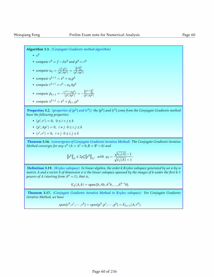
Properties 3.2. (properties of pk and rk) the pk and rk come from the Conjugate Gradients methodhave the following properties:

• (pj ,rj) = 0, 0 ≤ i < j ≤ k

• (pi ,Apj) = 0, i , j 0 ≤ i, j ≤ k

• (r i ,rj) = 0, i , j 0 ≤ i, j ≤ k

Theorem 3.16. (convergence of Conjugate Gradients iterative Method) The Conjugate Gradients iterativeMethod converges for any x0 (A= A∗ > 0,B= B∗ > 0) and

∥∥∥ek∥∥∥A≤ 2ρn0

∥∥∥e0∥∥∥A

, with ρ0 =

√κ2(A)− 1√κ2(A) + 1

.

Definition 3.19. (Krylov subspace) In linear algebra, the order-k Krylov subspace generated by an n-by-nmatrix A and a vector b of dimension n is the linear subspace spanned by the images of b under the first k-1powers of A (starting from A0 = I), that is,

Kk(A,b) = span b,Ab,A2b, . . . ,Ak−1b.

Theorem 3.17. (Conjugate Gradients iterative Method in Krylov subspace) For Conjugate Gradientsiterative Method, we have

spanr0,r1, · · · ,rk= spanp0,p1, · · · ,pk= Kk+1(A,r0).

Page 60 of 236


3.6 Problems

Problem 3.1. (Prelim Jan. 2011#1) Consider a linear system Ax = b with A ∈Rn×n. Richardson’s methodis an iterative method

Mxk+1 = Nxk + b

withM = 1w ,N =M−A= 1

w I−A, where w is a damping factor chosen to make M approximate A as well aspossible. Suppose A is positive definite and w > 0. Let λ1 and λn denote the smallest and largest eigenvalueof A.

1. Prove that Richardson’s method converges if and only if w < 2λn

.

2. Prove that the optimal value of w is w0 =2

λ1+λn.

Solution. 1. Since M = 1w ,N =M −A= 1

w I −A, then we have

xk+1 = (I −wA)xk + bw.

So TR = I − wA, From the sufficient and & necessary condition for convergence, we should haveρ(TR) < 1. Since λi are the eigenvalue of A, then we have 1 − λiw are the eigenvalues of TR. HenceRichardson’s method converges if and only if |1−λiw| < 1, i.e

−1 < 1−λnw < · · · < 1−λ1w < 1,

i.e. w < 2λn

.

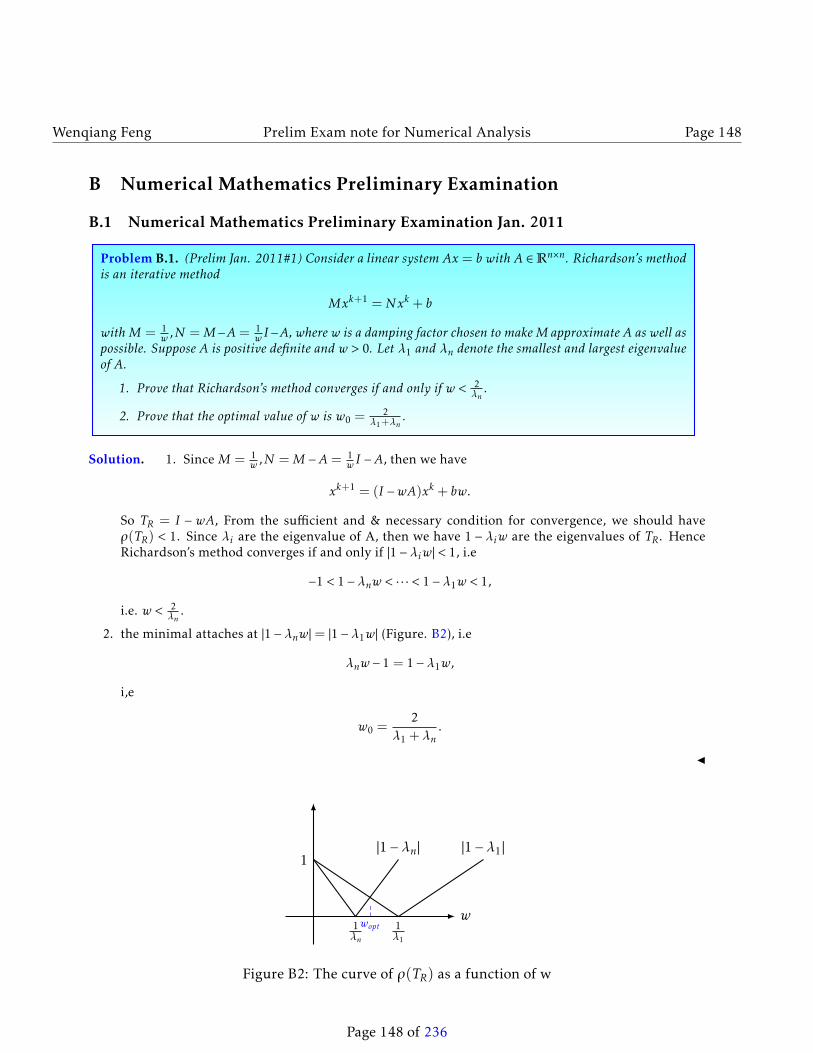
2. the minimal attaches at |1−λnw|= |1−λ1w| (Figure. B2), i.e

λnw − 1 = 1−λ1w,

i,e

w0 =2

λ1 +λn.

J

woptw

1

1λ1

|1−λ1|

1λn

|1−λn|

Figure 2: The curve of ρ(TR) as a function of w

Page 61 of 236


Problem 3.2. (Prelim Aug. 2010#3) Suppose that A ∈Rn×n is SPD and b ∈Rn is given. Then nth Krylovsubspace us defined as

Kn :=⟨b,Ab,A2b, · · · ,Ak−1b

⟩.

Letxj

n−1

j=0,x0 = 0, denote the sequence of vectors generated by the conjugate gradient algorithm. Prove

that if the method has not already converged after n − 1 iterations, i.e. rn−1 = b −Axn−1 , 0, then the nth

iterate xn us the unique vector in Kn that minimizes

φ(y) =∥∥∥x∗ − y∥∥∥2

A,

where x∗ = A−1b.

Solution. J

Problem 3.3. (Prelim Jan. 2011#1)

Solution. J

Page 62 of 236


4 Eigenvalue Problems

Definition 4.1. (Gerschgorin disks) Let A ∈ Cn×n, the Gerschgorin disks of A are

Di = ξ ∈ C : |ξ − aii | <Ri where Ri =∑i,j

|aij |.

Theorem 4.1. Every eigenvalue of A lies within at least one of the Gerschgorin discs Di

Proof. Let λ be an eigenvalue of A and let x = (xj) be a corresponding eigenvector. Let i ∈ 1, · · · ,n bechosen so that |xi | = maxj |xj |. (That is to say, choose i so that xi is the largest (in absolute value) numberin the vector x) Then |xi | > 0, otherwise x = 0. Since x is an eigenvector, Ax = λx, and thus:∑

j

aijxj = λxi ∀i ∈ 1, . . . ,n.

So, splitting the sum, we get ∑j,i

aijxj = λxi − aiixi .

We may then divide both sides by xi (choosing i as we explained, we can be sure that xi , 0) and take theabsolute value to obtain

|λ− aii |=∣∣∣∣∣∣∑j,i aijxjxi

∣∣∣∣∣∣ ≤∑j,i

∣∣∣∣∣aijxjxi

∣∣∣∣∣ ≤∑j,i

|aij |= Ri

where the last inequality is valid because ∣∣∣∣∣xjxi∣∣∣∣∣ ≤ 1 for j , i.

Corollary 4.1. The eigenvalues of A must also lie within the Gerschgorin discs Di corresponding to thecolumns of A.

Proof. Apply the Theorem to AT .

Definition 4.2. (Reyleigh Quotient) Let A ∈Rn×n, x ∈Rn. The Reyleigh Quotient is

R(x) =(Ax,x)(x,x)

.

Remark 4.1. If x is an eigenvector of A, then Ax = λx and

R(x) =(Ax,x)(x,x)

= λ.

Page 63 of 236


Properties 4.1. (properties of Reyleigh Quotient) Reyleigh Quotient has the following properties:

1.

∇R(x) = 2(x,x)

[Ax −R(x)x]

2. R(x) minimizes

f (α) = ‖Ax −αx‖2 .

Proof. 1. From the definition of the gradient, we have

∇R(x) =[∂r(x)

∂x1,∂r(x)

∂x2, · · · ,

∂r(x)

∂xn

].

By using the quotient rule, we have

∂r(x)

∂xi=

∂∂xi

((Ax,x)(x,x)

)=

∂∂xi

(xTAx

xT x

)=

∂∂xi

(xTAx

)xT x − xTAx ∂

∂xi

(xT x

)(xT x)2 ,

where∂∂xi

(xTAx

)=

∂∂xi

(xT

)Ax+ xT

∂∂xi

(Ax)

= [0, · · · ,0,1i,0, · · · ,0]Ax+ xTA

0...010...0

i

= (Ax)i + (Ax)i = 2 (Ax)i .

Similarly,

∂∂xi

(xT x

)=

∂∂xi

(xT

)x+ xT

∂∂xi

(x)

= [0, · · · ,0,1i,0, · · · ,0]x+ xT

0...010...0

i

= 2xi .

Therefore, we have

∂r(x)

∂xi=

2 (Ax)ixT x

− xTAx2xi(xT x)2

=2xT x

((Ax)i −R(x)xi) .

Page 64 of 236


Hence

∇R(x) = 2xT x

(Ax −R(x)x) =2

(x,x)(Ax −R(x)x) .

2. let

g(α) = ‖Ax −αx‖22 .

Then,

g(α) = (Ax −αx,Ax −αx) = (Ax,Ax)− 2α(Ax,x) +α2(x,x),

and

g ′(α) = −2(Ax,x) + 2α(x,x),

when R(x) minimizes

f (α) = ‖Ax −αx‖2

, then g ′(α) = 0, i.e.

α =(Ax,x)(x,x)

=R(x).

4.1 Schur algorithm

Algorithm 4.1. (Schur algorithm)

• A0 = A=Q ∗UQ

• compute Ak =Q−1k Ak−1Qk

4.2 QR algorithm

Algorithm 4.2. (QR algorithm)

• A0 = A

• compute QkRk = Ak−1

• compute Ak = RkQk

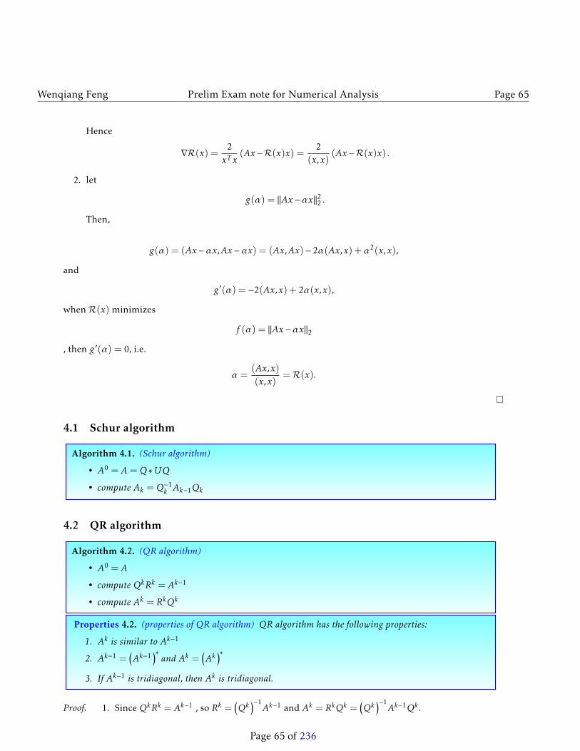
Properties 4.2. (properties of QR algorithm) QR algorithm has the following properties:

1. Ak is similar to Ak−1

2. Ak−1 =(Ak−1

)∗and Ak =

(Ak

)∗3. If Ak−1 is tridiagonal, then Ak is tridiagonal.

Proof. 1. Since QkRk = Ak−1 , so Rk =(Qk

)−1Ak−1 and Ak = RkQk =

(Qk

)−1Ak−1Qk .

Page 65 of 236


2. Since Q is unitary, so Q∗ =Q−1 and A= A∗, so(Ak

)∗=

((Qk

)−1Ak−1Qk

)∗=

(Qk

)∗ (Ak−1

)∗ ((Qk

)−1)∗=

(Qk

)−1 (Ak−1

)∗ (Qk

)=

(Qk

)−1Ak−1

(Qk

)= Ak .

Similarly, (Ak−1

)∗=

(QkAk

(Qk

)−1)∗=QkAk

(Qk

)−1= Ak−1.

3. since Ak is similar to Ak−1.

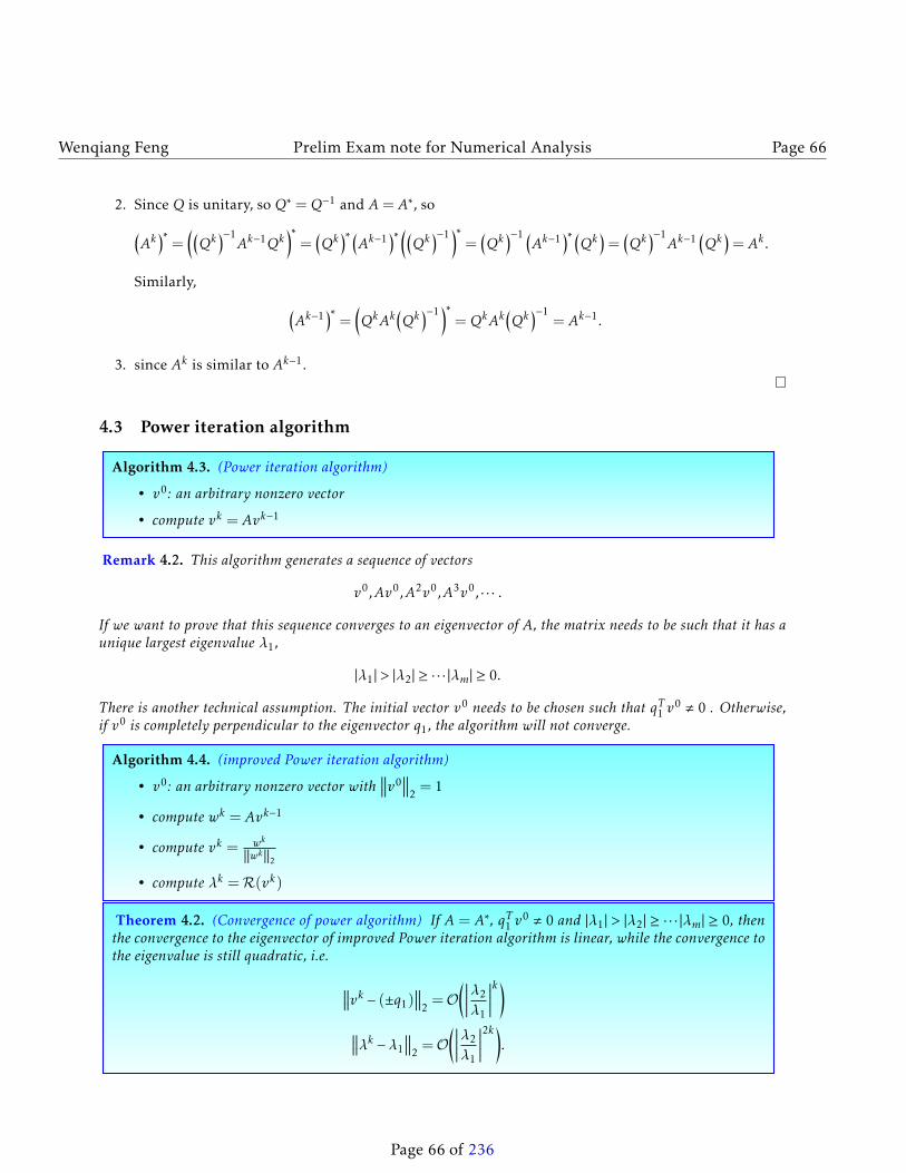
4.3 Power iteration algorithm

Algorithm 4.3. (Power iteration algorithm)

• v0: an arbitrary nonzero vector

• compute vk = Avk−1

Remark 4.2. This algorithm generates a sequence of vectors

v0,Av0,A2v0,A3v0, · · · .

If we want to prove that this sequence converges to an eigenvector of A, the matrix needs to be such that it has aunique largest eigenvalue λ1,

|λ1| > |λ2| ≥ · · · |λm| ≥ 0.

There is another technical assumption. The initial vector v0 needs to be chosen such that qT1 v0 , 0 . Otherwise,

if v0 is completely perpendicular to the eigenvector q1, the algorithm will not converge.

Algorithm 4.4. (improved Power iteration algorithm)

• v0: an arbitrary nonzero vector with∥∥∥v0

∥∥∥2= 1

• compute wk = Avk−1

• compute vk = wk

‖wk‖2• compute λk =R(vk)

Theorem 4.2. (Convergence of power algorithm) If A = A∗, qT1 v0 , 0 and |λ1| > |λ2| ≥ · · · |λm| ≥ 0, then

the convergence to the eigenvector of improved Power iteration algorithm is linear, while the convergence tothe eigenvalue is still quadratic, i.e.

∥∥∥vk − (±q1)∥∥∥

2= O

(∣∣∣∣∣λ2

λ1

∣∣∣∣∣k)∥∥∥λk −λ1

∥∥∥2= O

(∣∣∣∣∣λ2

λ1

∣∣∣∣∣2k).

Page 66 of 236


Proof. let q1,q2, · · · ,qn be the orthogonal basis of R. Then v0 can be rewritten as

v0 =∑

αjqj .

Moreover, following the power algorithm, we have

w1 = Av0 =∑

αjAqj =∑

αjλjqj .(Aqj = λjqj)

v1 =

∑αjλjqj√∑α2j λ

2j

w2 = Av1 =

∑αjλjAqj√∑α2j λ

2j

=

∑αjλ

2j qj√∑

α2j λ

2j

v2 =

∑αjλ

2j qj√∑

α2j λ

2·2j

· · ·

wk =

∑αjλ

kj qj√∑

α2j λ

2·(k−1)j

vk =

∑αjλ

kj qj√∑

α2j λ

2·kj

.

vk can be rewritten as

vk =

∑αjλ

kj qj√∑

α2j λ

2·kj

=α1λ

k1q1 +

∑j>1αjλ

kj qj√

α21λ

2k1 +

∑j>1α

2j λ

2kj

=α1λ

k1

|α1λk1|·q1 +

∑j>1

αjα1

(λjλ1

)kqj√

1+∑j>1

( αjα1

)2(λjλ1

)2k

= ±1q1 +

∑j>1

αjα1

(λjλ1

)kqj√

1+∑j>1

( αjα1

)2(λjλ1

)2k.

Therefore, ∥∥∥vk − (±q1)∥∥∥

2≤

∣∣∣∣∣∣∣∣∑j>1

αjα1

(λjλ1

)kqj

∣∣∣∣∣∣∣∣ ≤ C(∣∣∣∣∣λ2

λ1

∣∣∣∣∣)k = O(∣∣∣∣∣λ2

λ1

∣∣∣∣∣k).From Taylor formula ∥∥∥λk −λ1

∥∥∥2= |R(vk)−R(q1)|= O

∥∥∥vk − q1

∥∥∥2

2= O

(∣∣∣∣∣λ2

λ1

∣∣∣∣∣2k).Remark 4.3. This shows that the speed of convergence depends on the gap between the two largest eigenvalues

of A. In particular, if the largest eigenvalue of A were complex (which it can’t be for the real symmetric matriceswe are considering), then λ2 = λ1 and the algorithm would not converge at all.

Page 67 of 236


4.4 Inverse Power iteration algorithm

Algorithm 4.5. (inverse Power iteration algorithm)


∥∥∥2= 1

• compute wk = A−1vk−1

• compute vk = wk


Algorithm 4.6. (Improved inverse Power iteration algorithm)


∥∥∥2= 1

• compute wk = (A−µI)−1vk−1

• compute vk = wk


Remark 4.4. Improved inverse Power iteration algorithm is a shift µ.

Algorithm 4.7. (Rayleigh Quotient Iteration iteration algorithm)


∥∥∥2= 1

• compute λ0 =R(v0)

• compute wk = (A−λk−1I)−1vk−1

• compute vk = wk


Theorem 4.3. (Convergence of power algorithm) If A = A∗, qT1 v0 , 0 and |λ1| > |λ2| ≥ · · · |λm| ≥ 0, If we

update the estimate µ for the eigenvalue with the Rayleigh quotient at each iteration we can get a cubicallyconvergent algorithm, i.e. ∥∥∥vk+1 − (±qJ )

∥∥∥2= O

(∥∥∥vk − (±qJ )∥∥∥3

2

)∥∥∥λk −λJ∥∥∥2

= O(|λk −λJ |3

).

4.5 Problems

Problem 4.1. (Prelim Aug. 2013#1)

Solution. J

Page 68 of 236


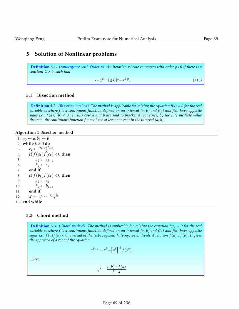
5 Solution of Nonlinear problems

Definition 5.1. (convergence with Order p) An iterative scheme converges with order p>0 if there is aconstant C > 0, such that

|x − xk+1| ≤ C|x − xk |p. (118)

5.1 Bisection method

Definition 5.2. (Bisection method) The method is applicable for solving the equation f(x) = 0 for the realvariable x, where f is a continuous function defined on an interval [a, b] and f(a) and f(b) have oppositesigns i.e. f (a)f (b) < 0. In this case a and b are said to bracket a root since, by the intermediate valuetheorem, the continuous function f must have at least one root in the interval (a, b).

Algorithm 1 Bisection method1: a0← a,b0← b2: while k > 0 do3: ck←

ak−1+bk−12

4: if f (ak)f (ck) < 0 then5: ak← ak−16: bk← ck7: end if8: if f (bk)f (ck) < 0 then9: ak← ck

10: bk← bk−111: end if12: xk← ck← ak+bk

213: end while

5.2 Chord method

Definition 5.3. (Chord method) The method is applicable for solving the equation f(x) = 0 for the realvariable x, where f is a continuous function defined on an interval [a, b] and f(a) and f(b) have oppositesigns i.e. f (a)f (b) < 0. Instead of the [a,b] segment halving, we?ll divide it relation f (a) : f (b), It givesthe approach of a root of the equation

xk+1 = xk −[ηk

]−1f (xk).

where

ηk =f (b)− f (a)

b − a

Page 69 of 236


Algorithm 2 Chord method

1: x1 = a− f (a)f (b)−f (a) (b − a), x0 = 0

2: ηk = f (b)−f (a)b−a

3: while |xk+1 − xk | < ε do4: xk+1← xk −

[ηk

]−1f (xk)

5: end while

5.3 Secant method

Definition 5.4. (Secant method) The method is applicable for solving the equation f(x) = 0 for the realvariable x, where f is a continuous function defined on an interval [a, b] and f(a) and f(b) have oppositesigns i.e. f (a)f (b) < 0. Instead of the [a,b] segment halving, we?ll divide it relation f (xk) : f (xk−1), Itgives the approach of a root of the equation

xk+1 = xk −[ηk

]−1f (xk).

where

ηk =f (xk)− f (xk−1)

xk − xk−1

Algorithm 3 Secant method

1: x1 = a− f (a)f (b)−f (a) (b − a)

2: ηk = f (xk)−f (xk−1)xk−xk−1 ,x0 = 0

3: while |xk+1 − xk | < ε do4: xk+1← xk −

[ηk

]−1f (xk)

5: end while

5.4 Newton’s method

Definition 5.5. (Newton’s method) The method is applicable for solving the equation f(x) = 0 for the realvariable x, where f is a continuous function defined on an interval [a, b] and f(a) and f(b) have oppositesigns i.e. f (a)f (b) < 0. Instead of the [a,b] segment halving, we?ll divide it relation f ′(xk), It gives theapproach of a root of the equation

xk+1 = xk −[ηk

]−1f (xk).

where

ηk = f ′(xk)

Remark 5.1. This scheme needs f ′(xk) , 0.

Page 70 of 236


Algorithm 4 Newton’s method

1: x1 = a− f (a)f (b)−f (a) (b − a)

2: ηk = f ′(xk),x0 = 03: while |xk+1 − xk | < ε do4: xk+1← xk −

[ηk

]−1f (xk)

5: end while

Theorem 5.1. (convergence of Newton’s method) Let f ∈ C2,f (x∗) = 0,f ′(x) , 0 and f ′′(x∗) is boundedin a neighborhood of x∗. Provide x0 is sufficient close to x∗, then newton’s method converges quadratically,i.e. ∣∣∣xk+1 − x∗

∣∣∣ ≤ C ∣∣∣xk − x∗∣∣∣2 .

Proof. Let x∗ be the root of f (x). From the Taylor expansion, we know

0 = f (x∗) = f (xk) + f ′(xk)(x∗ − xk) + 12f ′′(θ)(x∗ − xk)2,

where θ is between x∗ and xk . Define ek = x∗ − xk , then

0 = f (x∗) = f (xk) + f ′(xk)(ek) +12f ′′(θ)(ek)2.

so [f ′(xk)

]−1f (xk) = −(ek)− 1

2

[f ′(xk)

]−1f ′′(θ)(ek)2.

From the Newton’s scheme, we havexk+1 = xk −[f ′(xk)

]−1f (xk)

x∗ = x∗

So,

ek+1 = ek +[f ′(xk)

]−1f (xk) = −1

2

[f ′(xk)

]−1f ′′(θ)(ek)2,

i.e.

ek+1 = −f ′′(θ)

2[f ′(xk)

] (ek)2,

By assumption, there is a neighborhood of x, such that∣∣∣f (z)∣∣∣ ≤ C1,∣∣∣f ′(z)∣∣∣ ≤ C2,

Therefore, ∣∣∣ek+1∣∣∣ ≤ ∣∣∣f ′′(θ)∣∣∣∣∣∣∣2 [

f ′(xk)]∣∣∣∣ (ek)2 ≤ C1

2C2

∣∣∣ek ∣∣∣2 .

This implies ∣∣∣xk+1 − x∗∣∣∣ ≤ C ∣∣∣xk − x∗∣∣∣2 .

Page 71 of 236


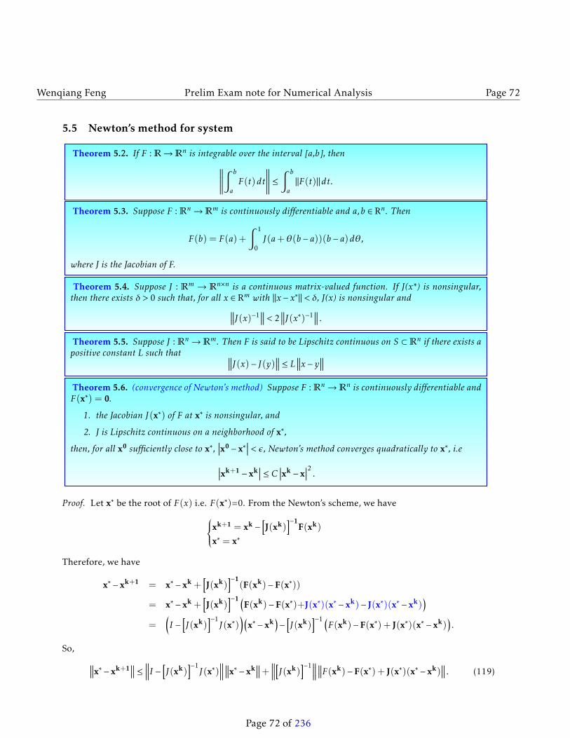
5.5 Newton’s method for system

Theorem 5.2. If F : R→Rn is integrable over the interval [a,b], then∥∥∥∥∥∥∫ b

aF(t)dt

∥∥∥∥∥∥ ≤∫ b

a‖F(t)‖dt.

Theorem 5.3. Suppose F : Rn→Rm is continuously differentiable and a,b ∈ Rn. Then

F(b) = F(a) +

∫ 1

0J(a+θ(b − a))(b − a)dθ,

where J is the Jacobian of F.

Theorem 5.4. Suppose J : Rm → Rn×n is a continuous matrix-valued function. If J(x*) is nonsingular,then there exists δ > 0 such that, for all x ∈ Rm with ‖x − x∗‖ < δ, J(x) is nonsingular and∥∥∥J(x)−1

∥∥∥ < 2∥∥∥J(x∗)−1

∥∥∥ .

Theorem 5.5. Suppose J : Rn→Rm. Then F is said to be Lipschitz continuous on S ⊂Rn if there exists apositive constant L such that ∥∥∥J(x)− J(y)∥∥∥ ≤ L∥∥∥x − y∥∥∥Theorem 5.6. (convergence of Newton’s method) Suppose F : Rn→Rn is continuously differentiable andF(x∗) = 0.

1. the Jacobian J(x∗) of F at x∗ is nonsingular, and

2. J is Lipschitz continuous on a neighborhood of x∗,

then, for all x0 sufficiently close to x∗,∣∣∣x0 − x∗

∣∣∣ < ε, Newton’s method converges quadratically to x∗, i.e∣∣∣xk+1 − xk∣∣∣ ≤ C ∣∣∣xk − x

∣∣∣2 .

Proof. Let x∗ be the root of F(x) i.e. F(x∗)=0. From the Newton’s scheme, we havexk+1 = xk −[J(xk)

]−1F(xk)

x∗ = x∗

Therefore, we have

x∗ − xk+1 = x∗ − xk +[J(xk)

]−1(F(xk)−F(x∗))

= x∗ − xk +[J(xk)

]−1 (F(xk)−F(x∗)+J(x∗)(x∗ − xk)− J(x∗)(x∗ − xk)

)=

(I −

[J(xk)

]−1J(x∗)

)(x∗ − xk

)−[J(xk)

]−1 (F(xk)−F(x∗) + J(x∗)(x∗ − xk)

).

So, ∥∥∥x∗ − xk+1∥∥∥ ≤ ∥∥∥∥I − [J(xk)

]−1J(x∗)

∥∥∥∥∥∥∥x∗ − xk∥∥∥+ ∥∥∥∥[J(xk)

]−1∥∥∥∥∥∥∥F(xk)−F(x∗) + J(x∗)(x∗ − xk)∥∥∥ . (119)

Page 72 of 236


Now, we will estimate∥∥∥∥I − [J(xk)

]−1J(x∗)

∥∥∥∥ and∥∥∥F(xk)−F(x∗) + J(x∗)(x∗ − xk)

∥∥∥.∥∥∥∥I − [J(xk)]−1J(x∗)

∥∥∥∥ =∥∥∥∥[J(xk)

]−1[J(xk)

]−[J(xk)

]−1J(x∗)

∥∥∥∥=

∥∥∥∥[J(xk)]−1 (

J(xk)− J(x∗))∥∥∥∥ (120)

≤∥∥∥∥[J(xk)

]−1∥∥∥∥∥∥∥J(xk)− J(x∗)∥∥∥

≤ L∥∥∥∥[J(xk)

]−1∥∥∥∥∥∥∥x∗ − xk∥∥∥ .

In the last step of the above equation, we use the J is Lipschitz continuous(If J is not Lipschitz contin-uous, we can only get the Newton method converges linearly to x∗). Since F : Rn → Rn is continuouslydifferentiable, therefore

F(b) = F(a) +

∫ 1

0J(a+θ(b − a))(b − a)dθ.

So

F(xk) = F(x∗) +∫ 1

0J(x∗+θ(xk − x∗))(xk − x∗)dθ

= F(x∗) +∫ 1

0J(x∗+θ(xk − x∗))(xk − x∗) + J(x∗)(x∗ − xk)− J(x∗)(x∗ − xk)dθ

= F(x∗)− J(x∗)(x∗ − xk) +

∫ 1

0J(x∗+θ(xk − x∗))(xk − x∗) + J(x∗)(x∗ − xk)dθ

Hence

F(xk)−F(x∗) + J(x∗)(x∗ − xk) =

∫ 1

0J(x∗+θ(xk − x∗))(xk − x∗) + J(x∗)(x∗ − xk)dθ.

So, ∥∥∥F(xk)−F(x∗) + J(x∗)(x∗ − xk)∥∥∥ =

∥∥∥∥∥∥∫ 1

0J(x∗+θ(xk − x∗))(xk − x∗) + J(x∗)(x∗ − xk)dθ

∥∥∥∥∥∥≤

∫ 1

0

∥∥∥J(x∗+θ(xk − x∗))(xk − x∗) + J(x∗)(x∗ − xk)∥∥∥dθ

≤∫ 1

0

∥∥∥J(x∗+θ(xk − x∗))− J(x∗)∥∥∥∥∥∥(x∗ − xk)

∥∥∥dθ (121)

≤∫ 1

0Lθ

∥∥∥(x∗ − xk)∥∥∥2dθ

≤ 12L∥∥∥(x∗ − xk)

∥∥∥2.

From (119), (120) and (121), we have∥∥∥x∗ − xk+1∥∥∥ ≤ 3

2L∥∥∥∥[J(xk)

]−1∥∥∥∥∥∥∥x∗ − xk∥∥∥2 ≤ 3L

∥∥∥[J(x∗)]−1∥∥∥∥∥∥x∗ − xk

∥∥∥2. (122)

Page 73 of 236


Remark 5.2. From the last step of the above proof process, we can get the condition of ε. such as, If∥∥∥x∗ − xk∥∥∥ ≤ 1

L∥∥∥[J(x∗)]−1

∥∥∥ ,

then ∥∥∥x∗ − xk+1∥∥∥ ≤ 1

2

∥∥∥x∗ − xk∥∥∥ . (123)

5.6 Fixed point method

In fact, Chord, scant and Newton’s method can be consider as fixed point iterative, since

xk+1 = xk −[ηk

]−1f (xk) = φ(xk).

Theorem 5.7. x is a fixed point of φ and Uδ = z : |x − z| ≤ δ. If φ is differentiable on Uδ and q < 1 such∣∣∣φ′(z)∣∣∣ ≤ q < 1 for all z ∈Uδ, then

1. φ(Uδ) ⊂Uδ2. φ is contraction.

5.7 Problems

Problem 5.1. (Prelim Jan. 2011#4) Let f : Ω ⊂ Rn → Rn be twice continuously differentiable. Supposex∗ ∈Ω is a solution of f (x) = 0, and the Jacobian matrix of f, denoted Jf , is invertible at x∗.

1. Prove that if x0 ∈Ω is sufficiently close to x∗, then the following iteration converges to x∗:

xk+1 = xk − Jf (x0)−1f (xk).

2. Prove that the convergence is typically only linear.

Solution. Let x∗ be the root of f(x) i.e. f(x∗)=0. From the Newton’s scheme, we havexk+1 = xk −[J(x0)

]−1f(xk)

x∗ = x∗

Therefore, we have

x∗ − xk+1 = x∗ − xk +[J(x0)

]−1(f(xk)− f(x∗))

= x∗ − xk −[J(x0)

]−1J(ξ)(x∗ − xk).

therefore ∣∣∣x∗ − xk+1∣∣∣ ≤ ∣∣∣∣∣1− J(ξ)

J(x0)

∣∣∣∣∣ ∣∣∣x∗ − xk∣∣∣

From theorem

Page 74 of 236


Theorem 5.8. Suppose J : Rm → Rn×n is a continuous matrix-valued function. If J(x*) is nonsingular, thenthere exists δ > 0 such that, for all x ∈ Rm with ‖x − x∗‖ < δ, J(x) is nonsingular and∥∥∥J(x)−1

∥∥∥ < 2∥∥∥J(x∗)−1

∥∥∥ .

we get ∣∣∣x∗ − xk+1∣∣∣ ≤ 1

2

∣∣∣x∗ − xk∣∣∣ .

Which also shows the convergence is typically only linear.J

Problem 5.2. (Prelim Aug. 2010#5) Assume that f : R → R,f ∈ C2(R),f ′(x) > 0 for all x ∈ R, andf ′′(x) > 0, for all x ∈R.

1. Suppose that a root ξ ∈ R exists. Prove that it is unique. Exhibit a function satisfying the assump-tions above that has no root.

2. Prove that for any starting guess x0 ∈ R, Newton’s method converges, and the convergence rate isquadratic.

Solution. 1. Let x1 and x2 are the two different roots. So, f (x1) = f (x2) = 0, then by Mean valuetheorem, we have that there exists η ∈ [x1,x2], such f ′(η) = 0 which contradicts f ′(x) > 0.

2. example f (x) = ex.

3. Let x∗ be the root of f (x). From the Taylor expansion, we know



0 = f (x∗) = f (xk) + f ′(xk)(ek) +12f ′′(θ)(ek)2.

so [f ′(xk)

]−1f (xk) = −(ek)− 1

2

[f ′(xk)

]−1f ′′(θ)(ek)2.


]−1f (xk)

x∗ = x∗

So,

ek+1 = ek +[f ′(xk)

]−1f (xk) = −1

2

[f ′(xk)

]−1f ′′(θ)(ek)2,

i.e.

ek+1 = −f ′′(θ)

2[f ′(xk)

] (ek)2,

By assumption, there is a neighborhood of x, such that∣∣∣f (z)∣∣∣ ≤ C1,∣∣∣f ′(z)∣∣∣ ≤ C2,

Page 75 of 236


Therefore,

∣∣∣ek+1∣∣∣ ≤ ∣∣∣f ′′(θ)∣∣∣∣∣∣∣2 [

f ′(xk)]∣∣∣∣ (ek)2 ≤ C1

2C2

∣∣∣ek ∣∣∣2 .


J

Problem 5.3. (Prelim Aug. 2010#4) Let f : Rn → R be twice continuously differentiable. Suppose x∗ isa isolated root of f and the Jacobian of f at x∗(J(x∗)) is non-singular. Determine conditions on ε so that if‖x0 − x∗‖2 < ε then the following iteration converges to x∗:

xk+1 = xk − Jf (x0)−1f (xk), k = 0,1,2, · · · .

Solution. J

Problem 5.4. (Prelim Aug. 2009#5) Consider the two-step Newton method

yk = xk −f (xk)

f ′(xk),xk+1 = yk −

f (yk)

f ′(xk)

for the solution of the equation f (x) = 0. Prove

1. If the method converges, then

limk→∞

xk+1 − x∗

(yk − x∗)(xk − x∗)=f ′′(xk)

f ′(xk),

where x∗ is the solution.

2. Prove the convergence is cubic, that is

limk→∞

xk+1 − x∗

(xk − x∗)3 =12

(f ′′(xk)

f ′(xk)

).

3. Would you say that this method is faster than Newton’s method given that its convergence is cubic?

Solution. 1. First, we will show that if xk ∈ [x − h,x+ h], then yk ∈ [x − h,x+ h]. By Taylor expansionformula, we have

0 = f (x∗) = f (xk) + f′(xk)(x

∗ − xk) +12!f ′′(ξk)(x

∗ − xk)2,

where ξ is between x and xk . Therefore, we have

f (xk) = −f ′(xk)(x∗ − xk)−12!f ′′(ξk)(x

∗ − xk)2.

Plugging the above equation to the first step of the Newton’s method, we have

yk = xk + (x∗ − xk) +12!f ′′(ξk)

f ′(xk)(x∗ − xk)2.

Page 76 of 236


then

yk − x∗ =12!f ′′(ξk)

f ′(xk)(x∗ − xk)2. (124)

Therefore, ∣∣∣yk − x∗∣∣∣= ∣∣∣∣∣ 12!f ′′(ξk)

f ′(xk)(x∗ − xk)2

∣∣∣∣∣ ≤ 12

∣∣∣∣∣ f ′′(ξk)f ′(xk)

∣∣∣∣∣ ∣∣∣(x∗ − xk)∣∣∣ ∣∣∣(x∗ − xk)∣∣∣ .Since we can choose the initial value very close to x∗, shah that∣∣∣∣∣ f ′′(ξ)f ′(xk)

∣∣∣∣∣ ∣∣∣(x∗ − xk)∣∣∣ ≤ 1

Then, we have that ∣∣∣yk − x∗∣∣∣ ≤ 12

∣∣∣(x∗ − xk)∣∣∣ .Hence, we proved the result, that is to say, if xk → x∗, then yk ,ξk → x∗.

2. Next, we will show if xk ∈ [x−h,x+h], then xk+1 ∈ [x−h,x+h]. From the second step of the Newton’sMethod, we have that

xk+1 − x∗ = yk − x∗ −f (yk)

f ′(xk)

=1

f ′(xk)((yk − x∗)f ′(xk)− f (yk))

=1

f ′(xk)[(yk − x∗)(f ′(xk)− f ′(x∗))− f (yk) + (yk − x∗)f ′(x∗)]

By mean value theorem, we have there exists ηk between x∗ and xk , such that

f ′(xk)− f ′(x∗) = f ′′ηk(xk − x∗),

and by Taylor expansion formula, we have

f (yk) = f (x∗) + f ′(x∗)(yk − x∗) +(yk − x∗)2

2f ′′(γk)

= f ′(x∗)(yk − x∗) +(yk − x∗)2

2f ′′(γk),

where γ is between yk and x∗. Plugging the above two equations to the second step of the Newton’smethod, we get

xk+1 − x∗ =1

f ′(xk)

[f ′′ηk(xk − x∗)(yk − x∗)− f ′(x∗)(yk − x∗)−

(yk − x∗)2

2f ′′(γk) + (yk − x∗)f ′(x∗)

]=

1f ′(xk)

[f ′′ηk(xk − x∗)(yk − x∗)−

(yk − x∗)2

2f ′′(γk)

]. (125)

Taking absolute values of the above equation, then we have∣∣∣xk+1 − x∗∣∣∣ =

∣∣∣∣∣∣ 1f ′(xk)

[f ′′ηk(xk − x∗)(yk − x∗)−

(yk − x∗)2

2f ′′(γk)

]∣∣∣∣∣∣≤ A |xk − x∗|

∣∣∣yk − x∗∣∣∣+ A2

∣∣∣yk − x∗∣∣∣ ∣∣∣yk − x∗∣∣∣≤ 1

2|xk − x∗|+

18|xk − x∗|=

58|xk − x∗| .

Hence, we proved the result, that is to say, if yk → x∗, then xk+1,ηk ,γk → x∗.

Page 77 of 236


3. Finally, we will prove the convergence order is cubic. From (215), we can get that

xk+1 − x∗

(xk − x∗)(yk − x∗)=

f ′′ηkf ′(xk)

−(yk − x∗)f ′′(γk)2(xk − x∗)f ′(xk)

.

By using (214), we have

xk+1 − x∗

(xk − x∗)(yk − x∗)=


− 14f ′′(ξk)

f ′(xk)(x∗ − xk)

f ′′(γk)

f ′(xk).

Taking limits gives

limk→∞

xk+1 − x∗

(xk − x∗)(yk − x∗)=f ′′(x∗)

f ′(x∗).

By using (214) again, we have

1yk − x∗

=2

(x∗ − xk)2f ′(xk)

f ′′(ξk).

Hence

limk→∞

xk+1 − x∗

(xk − x∗)3 =12

(f ′′(x∗)

f ′(x∗)

)2

.

J

Page 78 of 236


6 Euler Method

In this section, we focus on y′ = f (t,y),y(t0) = y0.

Where f is Lipschitz continuous w.r.t. the second variable, i.e

|f (t,x)− f (t,y)| ≤ λ|x − y|, λ > 0. (126)

In the following, We will let y(tn) to be the numerical approximation of yn and en = yn − y(tn) to be theerror.

Definition 6.1. (Order of the Method) A time stepping scheme

yn+1 = Φ(h,y0,y1, · · · ,yn) (127)

is of order of p ≥ 1 , if

yn+1 −Φ(h,y0,y1, · · · ,yn) = O(hp+1). (128)

Definition 6.2. (Convergence of the Method) A time stepping scheme

yn+1 = Φ(h,y0,y1, · · · ,yn) (129)

is convergent , if

limh→0

maxn

∥∥∥y(tn)− yn∥∥∥= 0. (130)

6.1 Euler’s method

Definition 6.3. (Forward Euler Methoda)

yn+1 = yn+ hf (tn,yn), n= 0,1,2, · · · . (131)

aForward Euler Method is explicit.

Theorem 6.1. (Forward Euler Method is of order 1 a) Forward Euler Method

y(tn+1) = y(tn) + hf (tn,y(tn)), (132)

is of order 1 .

aYou can also use multi-step theorem to derive it.

Proof. By the Taylor expansion,

y(tn+1) = y(tn) + hy′(tn) +O(h2). (133)

So,

y(tn+1)− y(tn)− hf (tn,y(tn)) = y(tn) + hy′(tn) +O(h2)− y(tn)− hf (tn,y(tn))

= y(tn) + hy′(tn) +O(h2)− y(tn)− hy′(tn) (134)

= O(h2).

Page 79 of 236


Therefore, Forward Euler Method (6.3) is order of 1 .

Theorem 6.2. (The convergence of Forward Euler Method) Forward Euler Method

y(tn+1) = y(tn) + hf (tn,y(tn)), (135)

is convergent.

Proof. From (134), we get

y(tn+1) = y(tn) + hf (tn,y(tn)) +O(h2), (136)

Subtracting (136) from (131), we get

en+1 = en+ h[f (tn,yn)− f (tn,y(tn))] + ch2. (137)

Since f is lipschitz continuous w.r.t. the second variable, then

|f (tn,yn)− f (tn,y(tn))| ≤ λ|yn − y(tn)|, λ > 0. (138)

Therefore, ∥∥∥en+1

∥∥∥ ≤ ‖en‖+ hλ‖en‖+ ch2

= (1+ hλ)‖en‖+ ch2. (139)

Claim:[2]

‖en‖ ≤cλh[(1+ hλ)n − 1],n= 0,1, · · · (140)

Proof for Claim (221): The proof is by induction on n.

1. when n= 0, en = 0, hence ‖en‖ ≤ cλh[(1+ hλ)n − 1],

2. Induction assumption:

‖en‖ ≤cλh[(1+ hλ)n − 1]

3. Induction steps: ∥∥∥en+1

∥∥∥ ≤ (1+ hλ)‖en‖+ ch2 (141)

≤ (1+ hλ)cλh[(1+ hλ)n − 1] + ch2 (142)

=cλh[(1+ hλ)n+1 − 1]. (143)

So, from the claim (221), we get ‖en‖ → 0, when h→ 0. Therefore Forward Euler Method is convergent.

Definition 6.4. (tableaux) The tableaux of Forward Euler method

0 01.

Page 80 of 236


Solution. Since, the Forward Euler method is as follows

yn+1 = yn+ hf (tn,yn),

then it can be rewritten as RK format, i.e.

ξ1 = ynyn+1 = yn+ hf (tn+ 0h,ξ1).

J

Definition 6.5. (Backward Euler Methodsa)

yn+1 = yn+ hf (tn+1,yn+1), n= 0,1,2, · · · . (144)

aBackward Euler Method is implicit.

Theorem 6.3. (backward Euler Method is of order 1 a) Backward Euler Method

y(tn+1) = y(tn) + hf (tn+1,y(tn+1)), (145)

is of order 1 .



y(tn+1) = y(tn) + hy′(tn) +O(h2) (146)

y′(tn+1) = y′(tn) +O(h). (147)

So,

y(tn+1)− y(tn)− hf (tn+1,y(tn+1))

= y(tn+1)− y(tn) + hy′(tn+1)

= y(tn) + hy′(tn) +O(h2)− y(tn)− h[y′(tn) +O(h)] (148)

= O(h2).

Therefore, Backward Euler Method (6.5) is order of 1 .

Theorem 6.4. (The convergence of Backward Euler Method) Backward Euler Method

y(tn+1) = y(tn) + hf (tn+1,y(tn+1)), (149)

is convergent.


y(tn+1) = y(tn) + hf (tn+1,y(tn+1)) +O(h2), (150)


en+1 = en+ h[f (tn+1,yn+1)− f (tn+1,y(tn+1))] + ch2. (151)

Page 81 of 236



|f (tn+1,yn+1)− f (tn+1,y(tn+1))| ≤ λ|yn+1 − y(tn+1)|, λ > 0. (152)


∥∥∥ ≤ ‖en‖+ hλ∥∥∥en+1

∥∥∥+ ch2. (153)

So,

(1− hλ)∥∥∥en+1

∥∥∥ ≤ ‖en‖+ ch2. (154)

So, by the Discrete Gronwall’s Inequality , we have

∥∥∥en+1

∥∥∥ ≤ ‖e0‖(1− hλ)n+1 + c

n∑k=0

h2

(1− hλ)n+k−1

= cn∑k=0

h2

(1− hλ)n+k−1(155)

≤ ch2(1+ hλ)(nh)/hλ(1− hλ→ 1+ hλ)

≤ cheT T .

So, from the claim (155), we get ‖en‖ → 0, when h→ 0. Therefore Backward Euler Method is convergent.

Definition 6.6. (tableaux) The tableaux of Backward Euler method

0 0 01 0 1

0 1.

Solution. Since, the Backward Euler method is as follows

yn+1 = yn+ hf (tn+1,yn+1),

then it can be rewritten as RK format, i.e.

ξ1 = ynξ2 = yn+ h [0f (tn+ 0h,ξ1) + 1f (tn+ 1h,ξ2)]

yn+1 = yn+ hf (tn+ h,ξ2).

J

6.2 Trapezoidal Method

Definition 6.7. (Trapezoidal Methoda)

yn+1 = yn+12h[f (tn,yn) + f (tn+1,yn+1)], n= 0,1,2, · · · . (156)

aTrapezoidal Method Method is a combination of Forward Euler Method and Backward Euler Method.

Page 82 of 236


Theorem 6.5. (Trapezoidal Method is of order 2 a) Trapezoidal Method

y(tn+1) = y(tn) +12h[f (tn,y(tn)) + f (tn+1,y(tn+1))], (157)

is of order 2 .



y(tn+1) = y(tn) + hy′(tn) +

12!h2y′′(tn) +O(h3) (158)

y′(tn+1) = y′(tn) + hy′′(tn) +O(h2). (159)

So,

y(tn+1)− y(tn) +12h[f (tn,y(tn)) + f (tn+1,y(tn+1))]

= y(tn+1)− y(tn) +12h[y′(tn) + y

′(tn+1)]

= y(tn) + hy′(tn) +

12!h2y′′(tn) +O(h3)− y(tn) +

12h[y′(tn) + y

′(tn) + hy′′(tn) +O(h2)] (160)

= O(h3).

Therefore, Trapezoidal Method (6.7) is order of 2 .

Theorem 6.6. (The convergence of Trapezoidal Method) Trapezoidal Method

y(tn+1) = y(tn) +12h[f (tn,y(tn)) + f (tn+1,y(tn+1))], (161)

is convergent.


y(tn+1) = y(tn) +12h[f (tn,y(tn)) + f (tn+1,y(tn+1))] +O(h3), (162)


en+1 = en+12h[f (tn,yn)− f (tn,y(tn)) + f (tn+1,yn+1)− f (tn+1,y(tn+1))] + ch

3. (163)


|f (tn,yn)− f (tn,y(tn))| ≤ λ|yn − y(tn)|, λ > 0, (164)

|f (tn+1,yn+1)− f (tn+1,y(tn+1))| ≤ λ|yn+1 − y(tn+1)|, λ > 0. (165)


∥∥∥ ≤ ‖en‖+12hλ(‖en‖+

∥∥∥en+1

∥∥∥) + ch3. (166)

Page 83 of 236


So,

(1− 12hλ)

∥∥∥en+1

∥∥∥ ≤ (1+12hλ)‖en‖+ ch3. (167)

Claim:[2]

‖en‖ ≤cλh2

1+ 12hλ

1− 12hλ

n − 1

,n= 0,1, · · · (168)


Then, we can make h small enough to such that 0 < hλ < 2, then

1+ 12hλ

1− 12hλ

= 1+1

1− 12hλ

≤∞∑`=0

1`!

hλ

1− 12hλ

` = exp

hλ

1− 12hλ

.

Therefore,

‖en‖ ≤cλh2

1+ 12hλ

1− 12hλ

n − 1

≤ cλh2

1+ 12hλ

1− 12hλ

n ≤ cλh2exp

nhλ

1− 12hλ

. (169)

This bound of true for every negative integer n such that nh < T . Therefore,

‖en‖ ≤cλh2exp

nhλ

1− 12hλ

≤ cλh2exp

T λ

1− 12hλ

. (170)

So, from the claim (170), we get ‖en‖ → 0, when h→ 0. Therefore Trapezoidal Method is convergent .

Definition 6.8. (tableaux) The tableaux of Trapezoidal method

0 0 01 1

212

12

12 .

6.3 Theta Method

Definition 6.9. (Theta Methoda)

yn+1 = yn+ h[θf (tn,yn) + (1−θ)f (tn+1,yn+1)], n= 0,1,2, · · · . (171)

aTheta Method is a general form of Forward Euler Method (θ = 1), Backward Euler Method (θ = 0) andTrapezoidal Method (θ = 1

2 ).

Definition 6.10. (tableaux) The tableaux of θ-method

0 0 01 θ 1-θ

θ 1-θ.

Page 84 of 236


Solution. Since, the θ-Method’s scheme is as follows,

yn+1 = yn+ h[θf (tn,yn) + (1−θ)f (tn+1,yn+1)], n= 0,1,2, · · · .

. Then, this scheme can be rewritten as RK-scheme, i.e.

ξ1 = ynξ2 = yn+ h [θf (tn+ 0h,ξ1) + (1−θ)(tn+ 1h,ξ2)]

yn+1 = yn+ h[θf (tn+ 0h,ξ1) + (1−θ)f (tn+ h,ξ2)]

So, the tableaux of θ-method is

0 0 01 θ 1-θ

θ 1-θ.

J

6.4 Midpoint Rule Method

Definition 6.11. (Midpoint Rule Method)

yn+1 = yn+ hf(tn+

12h,

12(yn+ yn+1)

). (172)

Theorem 6.7. (Midpoint Rule Method is of order 2) Midpoint Rule Method

y(tn+1) = y(tn) + hf(tn+

12h,

12(y(tn) + y(tn+1))

). (173)

is of order 2 .


y(tn+1) = y(tn) + hy′(tn) +

12!h2y′′(tn) +O(h3) (174)

f (x0 +∆x,y0 +∆y) = f (x0,y0) +

(∆x

∂∂x

+∆y∂∂y

)f (x0,y0) +O(h2). (175)

And chain rule

y′′ = f ′(t,y) =∂f (t,y)∂t

+∂f (t,y)∂y

f (t,y). (176)

So,

y(tn+1)− y(tn) + hf(tn+

12h,

12(y(tn) + y(tn+1))

)= y(tn) + hy

′(tn) +12!h2y′′(tn) +O(h3)− y(tn)

− h

(f (tn,yn) + (tn+

12h− tn)

∂f (tn,yn)∂t

+ (12(y(tn) + y(tn+1))− yn)

∂f (tn,yn)∂y

+O(h2)

)

Page 85 of 236


= hy′(tn) +12!h2y′′(tn) +O(h3)

−(hf (tn,yn) +

12h2∂f (tn,yn)

∂t+

12h2∂f (tn,yn)

∂y+O(h3)

)= hy′(tn) +

12!h2

(∂f (tn,yn)

∂t+∂f (tn,yn)

∂yy′(tn)

)−

(hy′(tn) +

12h2∂f (tn,yn)

∂t+

12h2∂f (tn,yn)

∂y+O(h3)

)= O(h3).

Therefore, Midpoint Rule Method (6.7) is order of 2 .

Theorem 6.8. (The convergence of Midpoint Rule Method) Midpoint Rule Method


12h,

12(y(tn) + y(tn+1))

), (177)

is convergent.



12h,

12(y(tn) + y(tn+1))

)+O(h3), (178)


en+1 = en+ h[f(tn+

12h,

12(y(tn) + y(tn+1))

)− f

(tn+

12h,

12(y(tn) + y(tn+1))

)]+ ch3. (179)

Since f is lipschitz continuous w.r.t. the second variable, then∣∣∣∣∣f (tn+

12h,

12(y(tn) + y(tn+1))

)− f

(tn+

12h,

12(y(tn) + y(tn+1))

)∣∣∣∣∣≤ 1

2λ|yn − y(tn) + yn+1 − y(tn+1)|, λ > 0. (180)


∥∥∥ ≤ ‖en‖+12hλ(‖en‖+

∥∥∥en+1

∥∥∥) + ch3. (181)

So,

(1− 12hλ)

∥∥∥en+1

∥∥∥ ≤ (1+12hλ)‖en‖+ ch3. (182)

Claim:[2]

‖en‖ ≤cλh2

1+ 12hλ

1− 12hλ

n − 1

,n= 0,1, · · · (183)


Page 86 of 236


Then, we can make h small enough to such that 0 < hλ < 2, then

1+ 12hλ

1− 12hλ

= 1+1

1− 12hλ

≤∞∑`=0

1`!

hλ

1− 12hλ

` = exp

hλ

1− 12hλ

.

Therefore,

‖en‖ ≤cλh2

1+ 12hλ

1− 12hλ

n − 1

≤ cλh2

1+ 12hλ

1− 12hλ

n ≤ cλh2exp

nhλ

1− 12hλ

. (184)

This bound of true for every negative integer n such that nh < T . Therefore,

‖en‖ ≤cλh2exp

nhλ

1− 12hλ

≤ cλh2exp

T λ

1− 12hλ

. (185)

So, from the claim (185), we get ‖en‖ → 0, when h→ 0. Therefore Midpoint Rule Method is convergent.

6.5 Problems


Solution. J

Page 87 of 236


7 Multistep Methond

7.1 The Adams Method

Definition 7.1. (s-step Adams-bashforth)

yn+s = yn+s−1 + hs−1∑m=0

bmf (tn+m,yn+m), (186)

where

bm = h−1∫ tn+s

tn+s−1

pm(τ)dτ = h−1∫ h

0pm(tn+s−1 + τ)dτ n= 0,1,2, · · · .

pm(t) = Πs−1l=0,l,m

t − tn+ltn+m − tn+l

, Lagrange interpolation polynomials .

(1-step Adams-bashforth)

yn+1 = yn+ hf (tn,yn),


yn+2 = yn+1 + h[3

2f (tn+1,yn+1)−

12f (tn,yn)

],


yn+3 = yn+2 + h[23

12f (tn+2,yn+2)−

43f (tn+1,yn+1) +

512f (tn,yn)

].

7.2 The Order and Convergence of Multistep Methods

Definition 7.2. (General s-step Method) The general s-step Method a can be written as

s∑m=0

amyn+m = hs∑

m=0

bmf(tn+m,yn+m). (187)

Where am,bm,m= 0, · · · ,s, are given constants, independent of h,n and original equation.

aif bs = 0 the method is explicit; otherwise it is implicit.

Page 88 of 236


Theorem 7.1. (s-step method convergent order) The multistep method (187) is of order p ≥ 1 if and onlyif there exists c , 0 s.t.

ρ(w)− σ (w) lnwa = c(w − 1)p+1 +O(|w − 1|p+2), w→ 1. (188)

Where,

ρ(w) :=s∑

m=0

amwm and σ (w) :=

s∑m=0

bmwm. (189)

aLet w = ξ + 1, then ln(1+ ξ) =∑∞n=0(−1)n ξ

n+1

n+1 = ξ − ξ2

2 + ξ3

3 −ξ4

4 + · · ·+ (−1)n ξn+1

n+1 + · · · ,ξ ∈ (−1,1).

Theorem 7.2. (s-step method convergent order) The multistep method (187) is of order p ≥ 1 if and onlyif

1.∑sm=0 am = 0, (i.e.ρ(1) = 0),

2.∑sm=0m

kam = k∑sm=0m

k−1bm,k = 1,2, · · · ,p,

3.∑sm=0m

p+1am , (p+ 1)∑sm=0m

pbm.

Where,

ρ(w) :=s∑

m=0

amwm and σ (w) :=

s∑m=0

bmwm. (190)

Lemma 7.1. (Root Condition) If the roots |λi | ≤ 1 for each i = 1, · · · ,m and all roots with value 1 aresimple root then the difference method is said to satisfy the root condition.

Theorem 7.3. (The Dahlquist equivalence theorem) The multistep method (187) is convergent if and onlyif

1. consistency: multistep method (187)is order of p ≥ 1 ,

2. stability: the polynomial ρ(w) satisfies the root condition .

7.3 Method of A-stable verification for Multistep Methods

Theorem 7.4. Explicit Multistep Methods can not be A-stable.

Theorem 7.5. (Dahlquist second barrier) The highest oder of an A-stable multistep method is 2 .

7.4 Problems

Problem 7.1. Find the order of the following quadrature formula.∫ 1

0f (τ)dτ =

16f (0) +

23f (

12) +

16f (1), Simpson Rule.

Solution. Since the quadrature formula (209) is order of p if it is exact for every f ∈ Pp−1. we can chose

Page 89 of 236


the simplest basis (1,τ ,τ2,τ3, · · · ,τp−1), and the order conditions read that

p∑j=1

bjcmj =

∫ b

aτmw(τ)dτ , m= 0,1, · · · ,p − 1. (191)

Checking the order condition by the following procedure,

1 =

∫ 1

01dτ =

16

1+23

1+16

1 = 1.

12=

∫ 1

0τdτ =

16

0+23

(12

)+

16

1 =12

.

13=

∫ 1

0τ2dτ =

16

02 +23

(12

)2+

16

12 =13

.

14=

∫ 1

0τ3dτ =

16

03 +23

(12

)3+

16

13 =14

.

15=

∫ 1

0τ4dτ ,

16

04 +23

(12

)4+

16

14 =5

24.

we can get the order of the Simpson rule quadrature formula is 4. J

Problem 7.2. Recall Simpson’s quadrature rule:∫ b

af (τ)dτ =

b − a6

[f (a) + 4f (

a+ b2

) + f (b)

]+O(|b − a|4), Simpson Rule.

Starting from the identity

y(tn+1)− y(tn−1) =

∫ tn+1

tn−1

f (s;y(s))ds. (192)

use Simpson’s rule to derive a 3-step method. Determine its order and whether it is convergent.

Solution. 1. The derivation of the a 3-step methodsince,

y(tn+1)− y(tn−1) =

∫ tn+1

tn−1

f (s;y(s))ds. (193)

Then,by Simpson’s quadrature rule, we have

y(tn+1)− y(tn−1) (194)

=

∫ tn+1

tn−1

f (s;y(s))ds. (195)

=tn+1 − tn−1

6

[f (tn−1;y(tn−1)) + 4f

( tn−1 + tn+1

2;y

( tn−1 + tn+1

2

))+ f (tn+1;y(tn+1))

](196)

=h3[f (tn−1;y(tn−1)) + 4f (tn;y (tn)) + f (tn+1;y(tn+1))] . (197)

Page 90 of 236


Therefore, the 3-step method deriving from Simpson’s rule is

y(tn+1) = y(tn−1) +h3[f (tn−1;y(tn−1)) + 4f (tn;y (tn)) + f (tn+1;y(tn+1))] . (198)

Or

y(tn+2)− y(tn) =h3[f (tn;y(tn)) + 4f (tn+1;y (tn+1)) + f (tn+2;y(tn+2))] . (199)

2. The order For our this problem

ρ(w) :=s∑

m=0

amwm = −1+w2 and σ (w) :=

s∑m=0

bmwm =

13+

43w+

13w2. (200)

By making the substitution with ξ = w − 1 i.e. w = ξ + 1, then

ρ(w) :=s∑

m=0

amwm = ξ2 + 2ξ and σ (w) :=

s∑m=0

bmwm =

13ξ2 + 2ξ + 2. (201)

So,

ρ(w)− σ (w)ln(w) = ξ2 + 2ξ − (2+ 2ξ +13ξ2)(ξ − ξ

2

2+ξ3

3· · · )

=

+2ξ +ξ2

−2ξ +ξ2 −23ξ

3

−2ξ2 +ξ3 −23ξ

4

−13ξ

3 + 16ξ

4 −19ξ

5

= −12ξ4 +O(ξ5).

Therefore, by the theorem

ρ(w)− σ (w)ln(w) = −12ξ4 +O(ξ5).

Hence, this scheme is order of 3.

3. The stability Since,

ρ(w) :=s∑

m=0

amwm = −1+w2 = (w − 1)(w+ 1). (202)

And w = ±1 are simple root which satisfy the root condition. Therefore, this scheme is stable.Hence, it is of order 3 and convergent. convergent J

Problem 7.3. Restricting your attention to scalar autonomous y′ = f (y), prove that the ERK method withtableau

012

12

12 0 1

21 0 0 1

16

13

13

16

is of order 4.

Page 91 of 236


Solution. J

Problem 7.4. (Prelim Jan. 2011#5) Consider

y′(t) = f (t,y(t)), t ≥ t0,y(t0) = y0,

where f : [t0, t∗]×R→R is continuous in its first variable and Lipschitz continuous in its second variable.Prove that Euler’s method converges.

Solution. The Euler’s scheme is as follows:

yn+1 = yn+ hf (tn,yn), n= 0,1,2, · · · . (203)

By the Taylor expansion,

y(tn+1) = y(tn) + hy′(tn) +O(h2).

So,



= O(h2).

Therefore, Forward Euler Method is order of 1 .From (219), we get



en+1 = en+ h[f (tn,yn)− f (tn,y(tn))] + ch2.


|f (tn,yn)− f (tn,y(tn))| ≤ λ|yn − y(tn)|, λ > 0.


∥∥∥ ≤ ‖en‖+ hλ‖en‖+ ch2

= (1+ hλ)‖en‖+ ch2.

Claim:[2]

‖en‖ ≤cλh[(1+ hλ)n − 1],n= 0,1, · · ·




‖en‖ ≤cλh[(1+ hλ)n − 1]

Page 92 of 236



∥∥∥ ≤ (1+ hλ)‖en‖+ ch2

≤ (1+ hλ)cλh[(1+ hλ)n − 1] + ch2

=cλh[(1+ hλ)n+1 − 1].

So, from the claim (221), we get ‖en‖ → 0, when h→ 0. Therefore Forward Euler Method is convergent .J

Problem 7.5. (Prelim Jan. 2011#6) Consider the scheme

yn+2 + yn+1 − 2yn = h (f (tn+2,yn+2) + f (tn+1,yn+1) + f (tn,yn))

for approximating the solution to

y′(t) = f (t,y(t)), t ≥ t0,y(t0) = y0,

what’s the order of the scheme? Is it a convergent scheme? Is it A-stable? Justify your answers.

Solution. For our this problem

ρ(w) :=s∑

m=0

amwm = −2+w+w2 and σ (w) :=

s∑m=0

bmwm = 1+w+w2. (206)


ρ(w) :=s∑

m=0


s∑m=0

bmwm = ξ2 + 3ξ + 3. (207)

So,

ρ(w)− σ (w)ln(w) = ξ2 + 3ξ − (3+ 3ξ + ξ2)(ξ − ξ2

2+ξ3

3· · · )

=

+3ξ +ξ2

−3ξ −3ξ2 −ξ3

+ 32ξ

2 + 32ξ

3 + 12ξ

4

−ξ3 −ξ4 −13ξ

5

= −12ξ2 +O(ξ3).


ρ(w)− σ (w)ln(w) = −12ξ2 +O(ξ3).

Hence, this scheme is order of 1. The stability Since,

ρ(w) :=s∑

m=0

amwm = −2+w+w2 = (w+ 2)(w − 1). (208)

And w = −1 or w = −2 which does not satisfy the root condition. Therefore, this scheme is not stable.Hence, it is also not A-stable.

J

Page 93 of 236


Problem 7.6. (Prelim Jan. 2011#4)

Solution. J

Page 94 of 236


8 Runge-Kutta Methods

8.1 Quadrature Formulas

Definition 8.1. (The Quadrature) The Quadrature is the procedure of replacing an integral with a finitesum.

Definition 8.2. (The Quadrature Formula) Let w be a nonnegative function in (a,b) s.t.

0 <∫ b

aw(τ)dτ <∞,

∣∣∣∣∣∣∫ b

aτ jw(τ)dτ

∣∣∣∣∣∣ <∞, j = 1,2, · · · .

Then, the quadrature formula is as following∫ b

af (τ)w(τ)dτ ≈

n∑j

bjf (cj). (209)

Remark 8.1. The quadrature formula (209) is order of p if it is exact for every f ∈Pp−1.

8.2 Explicit Runge-Kutta Formulas

Definition 8.3. (Explicit Runge-Kutta Formulas) Explicit Runge-Kutta is to integral from tn to tn+1 asfollows

y(tn+1) = y(tn) +

∫ tn+1

tn

f (τ ,y(τ))dτ

= y(tn) + h

∫ 1

0f (tn+ hτ ,y(tn+ hτ))dτ

and to replace the second integral by a quadrature, i.e.

yn+1 = yn+ hν∑j=1

bjf (tn+ cjh,y(tn+ cjh))

Specifically, we have

ξ1 = yn,

ξ2 = yn+ ha21f (tn,ξ1)

ξ3 = yn+ ha31f (tn+ c1h,ξ1) + ha32f (tn+ c2h,ξ2)

...

ξν = yn+ hν−1∑i=1

aνif (tn+ cih,ξi))


bjf (tn+ cjh,ξj)).

Page 95 of 236


Definition 8.4. (tableaux) The tableaux of REK

c AbT

where A is low triangular matrix.

Remark 8.2. by observing that the condition

j−1∑i=1

aj,i = cj , j = 2,3, · · · ,ν,

is necessary for order 1.

8.3 Implicit Runge-Kutta Formulas

Definition 8.5. (Implicit Runge-Kutta Formulas) Implicit Runge-Kutta use the following scheme

ξj = yn+ hν∑i=1

aj,if (tn+ cih,ξi), j = 1,2, · · · ,ν


bjf (tn+ cjh,ξj).

8.4 Method of A-stable verification for Runge-Kutta Method

Theorem 8.1. Explicit Runge-Kutta Methods can not be A-stable.

Theorem 8.2. necessary & sufficient A necessary & sufficient condition for A-stable Runge-Kutta methodis ∣∣∣r(z)∣∣∣ < 1, z ∈ C−,

where

r(z) = 1+ zbT (I − zA)−11.

8.5 Problems

Page 96 of 236


9 Finite Difference Method

Definition 9.1. (Discrete 2-norm) The discrete 2-norm is defined as follows

‖u‖22,h = hdN∑i=1

|ui |2,

where d is dimension.

Theorem 9.1. (Discrete maximum principle) Let A = tridiagai ,bi ,cini=1 ∈ Rn×n be a tridiagionalmatrix with the properties that

bi > 0, ai ,ci ≤ 0, ai + bi + ci = 0.

Prove the following maximum principle: If u ∈Rn is such that (Au)i=2,··· ,n−1 ≤ 0, then ui ≤maxu1,un.

Proof. Without loss generality, we assume uk ,k = 2, · · · ,n− 1 is the maximum value.

1. For (Au)i=2,··· ,n−1 < 0:I will use the method of contradiction to prove this case. Since (Au)i=2,··· ,n−1 < 0, so

akuk−1 + bkuk + ckuk+1 < 0.

Since ak + ck = −bk and ak < 0,ck < 0, so

akuk−1 − (ak + ck)uk + ckuk+1 = ak(uk−1 −uk) + ck(uk+1 −uk) ≥ 0.

This is contradiction to (Au)i=2,··· ,n−1 < 0. Therefore, If u ∈ Rn is such that (Au)i=2,··· ,n−1 < 0, thenui <maxu1,un.

2. For (Au)i=2,··· ,n−1 = 0:Since (Au)i=2,··· ,n−1 = 0, so

akuk−1 + bkuk + ckuk+1 = 0.

Since ak + ck = −bk , so

akuk−1 − (ak + ck)uk + ckuk+1 = ak(uk−1 −uk) + ck(uk+1 −uk) = 0.

And ak < 0,ck < 0,uk−1 −uk ≤ 0,uk+1 −uk ≤ 0, so uk−1 = uk = uk+1, that is to say, uk−1 and uk+1 is alsothe maximum points. Bu using the same argument again, we get uk−2 = uk−1 = uk = uk+1 = uk+2.Repeating the process, we get

u1 = u2 = · · ·= un−1 = un.

Therefore, If u ∈Rn is such that (Au)i=2,··· ,n−1 = 0, then ui ≤maxu1,un

Theorem 9.2. (Discrete Poincaré inequality) Let Ω= (0,1) and Ωh be a uniform grid of size h. If Y ∈ Uhis a mesh function on Ωh such that Y (0) = 0, then there is a constant C, independent of Y and h, for which

‖Y ‖2,h ≤ C∥∥∥δY ∥∥∥

2,h.

Page 97 of 236


Proof. I consider the following uniform partition (Figure. A1) of the interval (0,1) with N points.

x1 = 0 x2 xN−1 xN = 1

Figure 3: One dimension’s uniform partition

Since the discrete 2-norm is defined as follows

‖v‖22,h = hdN∑i=1

|vi |2,

where d is dimension. So, we have

‖v‖22,h = hN∑i=1

|vi |2,∥∥∥δv∥∥∥2

2,h= h

N∑i=2

∣∣∣∣vi−1 − vih

∣∣∣∣2 .

Since Y (0) = 0, i.e. Y1 = 0,

N∑i=2

(Yi−1 −Yi) = Y1 −YN = −YN .

Then, ∣∣∣∣∣∣∣N∑i=2

(Yi−1 −Yi)

∣∣∣∣∣∣∣= |YN |.and

|YN | ≤N∑i=2

|Yi−1 −Yi |=N∑i=2

h

∣∣∣∣∣Yi−1 −Yih

∣∣∣∣∣ ≤ N∑i=2

h2

1/2 N∑

i=2

∣∣∣∣∣Yi−1 −Yih

∣∣∣∣∣2

1/2

.

Therefore

|YK |2 ≤

K∑i=2

h2

K∑i=2

∣∣∣∣∣Yi−1 −Yih

∣∣∣∣∣2

= h2(K − 1)K∑i=2

∣∣∣∣∣Yi−1 −Yih

∣∣∣∣∣2.

1. When K = 2,

|Y2|2 ≤ h2∣∣∣∣∣Y1 −Y2

h

∣∣∣∣∣2 .

2. When K = 3,

|Y3|2 ≤ 2h2(∣∣∣∣∣Y1 −Y2

h

∣∣∣∣∣2 + ∣∣∣∣∣Y2 −Y3

h

∣∣∣∣∣2) .

Page 98 of 236


3. When K = N ,

|YN |2 ≤ (N − 1)h2(∣∣∣∣∣Y1 −Y2

h

∣∣∣∣∣2 + ∣∣∣∣∣Y2 −Y3

h

∣∣∣∣∣2 + · · ·+ ∣∣∣∣∣YN−1 −YNh

∣∣∣∣∣2) .

Sum over |Yi |2 from 2 to N, we get

N∑i=2

|Yi |2 ≤N (N − 1)

2h2

N∑i=2

∣∣∣∣∣Yi−1 −Yih

∣∣∣∣∣2.

Since Y1 = 0, so

N∑i=1

|Yi |2 ≤N (N − 1)

2h2

N∑i=2

∣∣∣∣∣Yi−1 −Yih

∣∣∣∣∣2.

And then

1(N − 1)2

N∑i=1

|Yi |2 ≤N

2(N − 1)h2

N∑i=2

∣∣∣∣∣Yi−1 −Yih

∣∣∣∣∣2 = (12+

12(N − 1)

)h2

N∑i=2

∣∣∣∣∣Yi−1 −Yih

∣∣∣∣∣2.

Since h= 1N−1 , so

h2N∑i=1

|Yi |2 ≤(

12+

12(N − 1)

)h2

N∑i=2

∣∣∣∣∣Yi−1 −Yih

∣∣∣∣∣2.

then

hN∑i=1

|Yi |2 ≤(

12+

12(N − 1)

)hN∑i=2

∣∣∣∣∣Yi−1 −Yih

∣∣∣∣∣2.

i.e,

‖Y ‖22,h ≤(

12+

12(N − 1)

)∥∥∥δY ∥∥∥22,h

.

since N ≥ 2, so

‖Y ‖22,h ≤∥∥∥δY ∥∥∥2

2,h.

Hence,

‖Y ‖2,h ≤ C∥∥∥δY ∥∥∥

2,h.

Theorem 9.3. (Von Neumann stability analysis method) For the difference scheme

Un+1j =

∑p∈N

αpUnj−p,

we have the corresponding Fourier transform is as follows

Un+1(ξ) =∑p∈N

αpe−ipξUn(ξ) := G(λ,ξ)Un(ξ).

Where λ = τh2 is CFL number and G(λ,ξ) is called Growth factor . If

∣∣∣G(λ,ξ)∣∣∣ ≤ 1, then the difference

scheme is stable.

Page 99 of 236


9.1 Problems

Problem 9.1. (Prelim Jan. 2011#7) Consider the Crank-Nicholson scheme applied to the diffusion equation

∂u∂t

=∂2u

∂x2

where t > 0,−∞ < x <∞.

1. Show that the amplification factor in the Von Neumann analysis of the scheme us

g(ξ) =1+ 1

2z

1− 12z

,z = 2∆t

∆x2 (cos(∆xξ)− 1).

2. Use the results of part 1 to show that the scheme is stable.

Solution. 1. The Crank-Nicholson scheme for the diffusion equation is

un+1j −unj∆t

=12

un+1j−1 − 2un+1

j + un+1j+1

∆x2 +unj−1 − 2unj + u

nj+1

∆x2

Let µ= ∆t

∆x2 , then the scheme can be rewrote as

un+1j = unj +

µ

2

(un+1j−1 − 2un+1

j + un+1j+1 + unj−1 − 2unj + u

nj+1

),

i.e.

−µ

2un+1j−1 + (1+ µ)un+1

j −µ

2un+1j+1 =

µ

2unj−1 + (1−µ)unj +

µ

2unj+1.

By using the Fourier transform, i.e.

un+1j = g(ξ)unj , unj = eij∆xξ ,

then we have

−µ

2g(ξ)unj−1 + (1+ µ)g(ξ)unj −

µ

2g(ξ)unj+1 =

µ

2unj−1 + (1−µ)unj +

µ

2unj+1.

And then

−µ

2g(ξ)ei(j−1)∆xξ + (1+ µ)g(ξ)eij∆xξ −

µ

2g(ξ)ei(j+1)∆xξ =

µ

2ei(j−1)∆xξ + (1−µ)eij∆xξ +

µ

2ei(j+1)∆xξ ,

i.e.

g(ξ)(−µ

2e−i∆xξ + (1+ µ)−

µ

2ei∆xξ

)ej∆xξ =

(µ2e−i∆xξ + (1−µ) +

µ

2ei∆xξ

)ej∆xξ ,

i.e.

g(ξ) (1+ µ−µcos(∆xξ)) = 1−µ+ µcos(∆xξ).

therefore,

g(ξ) =1−µ+ µcos(∆xξ)1+ µ−µcos(∆xξ)

.

hence

g(ξ) =1+ 1

2z

1− 12z

,z = 2∆t

∆x2 (cos(∆xξ)− 1).

Page 100 of 236


2. since z = 2 ∆t∆x2 (cos(∆xξ)− 1), then z < 0, then we have

1+12z < 1− 1

2z,

therefore g(ξ) < 1. Since −1 < 1, then

12z − 1 <

12z+ 1.

Therefore,

g(ξ) =1+ 1

2z

1− 12z

> −1.

hence∣∣∣g(ξ)∣∣∣ < 1. So, the scheme is stable.

J

Problem 9.2. (Prelim Jan. 2011#8) Consider the explicit scheme

un+1j = unj + µ

(unj−1 − 2unj + u

nj+1

)−bµ∆x

2

(unj+1 −u

nj−1

),0 ≤ n ≤N ,1 ≤ j ≤ L.

for the convention-diffusion problem∂u∂t =

∂2u∂x2 − b ∂u∂x for 0 ≤ x ≤ 1, 0 ≤ t ≤ t∗

u(0, t) = u(1, t) = 0 for 0 ≤ t ≤ t∗

u(x,0) = g(x) for 0 ≤ x ≤ 1,

where b > 0, µ = ∆t(∆x)2 ,∆x = 1

L+1 , and ∆t = t∗N . Prove that, under suitable restrictions on µ and ∆x, the

error grid function en satisfy the estimate

‖en‖∞ ≤ t∗C(∆t+∆x2

),

for all n such that n∆t ≤ t∗, where C > 0 is a constant.

Solution. Let u be the exact solution and unj = u(n∆t, j∆x). Then from Taylor Expansion, we have

un+1j = unj +∆t

∂∂tunj +

12(∆t)2 ∂

2

∂t2u(ξ1, j∆x), tn ≤ ξ1 ≤ tn+1,

unj−1 = unj −∆x∂∂xunj −

16(∆x)3 ∂

3

∂x3 unj +

124

(∆x)4 ∂4

∂x4 u(n∆t,ξ2), xj−1 ≤ ξ2 ≤ xj ,

unj+1 = unj +∆x∂∂xunj +

16(∆x)3 ∂

3

∂x3 unj +

124

(∆x)4 ∂4

∂x4 u(n∆t,ξ3), xj ≤ ξ3 ≤ xj+1.

Then the truncation error T of this scheme is

T =un+1j − unj∆t

−unj−1 − 2unj + u

nj+1

∆x2 + bunj+1 − u

nj−1

∆x= O(∆t+ (∆x)2).

Therefore

en+1j = enj + µ

(enj−1 − 2enj + e

nj+1

)−bµ∆x

2

(enj+1 − e

nj−1

)+ c∆t(∆t+ (∆x)2),

Page 101 of 236


i.e.

en+1j =

(µ+

bµ∆x

2

)enj−1 + (1− 2µ)enj +

(µ−

bµ∆x

2

)enj+1 + c∆t(∆t+ (∆x)2).

Then ∣∣∣∣en+1j

∣∣∣∣ ≤ ∣∣∣∣∣µ+ bµ∆x

2

∣∣∣∣∣ ∣∣∣∣enj−1

∣∣∣∣+ ∣∣∣(1− 2µ)∣∣∣ ∣∣∣∣enj ∣∣∣∣+ ∣∣∣∣∣µ− bµ∆x2

∣∣∣∣∣ ∣∣∣∣enj+1

∣∣∣∣+ c∆t(∆t+ (∆x)2).

Therefore∥∥∥∥en+1j

∥∥∥∥∞ ≤∣∣∣∣∣µ+ bµ∆x

2

∣∣∣∣∣∥∥∥∥enj−1

∥∥∥∥∞+∣∣∣(1− 2µ)

∣∣∣∥∥∥∥enj ∥∥∥∥∞+

∣∣∣∣∣µ− bµ∆x2

∣∣∣∣∣∥∥∥∥enj+1

∥∥∥∥∞+ c∆t(∆t+ (∆x)2).

∥∥∥en+1∥∥∥∞ ≤ ∣∣∣∣∣µ+ bµ∆x

2

∣∣∣∣∣‖en‖∞+∣∣∣(1− 2µ)

∣∣∣‖en‖∞+

∣∣∣∣∣µ− bµ∆x2

∣∣∣∣∣‖en‖∞+ c∆t(∆t+ (∆x)2).

If 1− 2µ ≥ 0 and µ− bµ∆x2 ≥ 0, i.e. µ ≤ 12 and 1− 1

2b∆x > 0, then∥∥∥en+1∥∥∥∞ ≤

(µ+

bµ∆x

2

)‖en‖∞+ ((1− 2µ))‖en‖∞+

(µ−

bµ∆x

2

)‖en‖∞+ c∆t(∆t+ (∆x)2)

= ‖en‖∞+ c∆t(∆t+ (∆x)2).

Then

‖en‖∞ ≤∥∥∥en−1

∥∥∥∞+ c∆t(∆t+ (∆x)2)

≤∥∥∥en−2

∥∥∥∞+ c2∆t(∆t+ (∆x)2)

≤...

≤∥∥∥e0

∥∥∥∞+ cn∆t(∆t+ (∆x)2)

= ct∗(∆t+ (∆x)2).

J

Problem 9.3. (Prelim Aug. 2010#8) Consider the Crank-Nicolson scheme

un+1j = unj +

µ

2

(un+1j−1 − 2un+1

j + un+1j+1 + unj−1 − 2unj + u

nj+1

)for approximating the solution to the heat equation ∂u

∂t =∂2u∂x2 on the intervals 0 ≤ x ≤ 1 and 0 ≤ t ≤ t∗ with

the boundary conditions u(0, t) = u(1, t) = 0.

1. Show that the scheme may be written in the form un+1 = Aun, where A ∈Rm×msym (the space of m×m

symmetric matrices) and

‖Ax‖2 ≤ ‖x‖2 ,

for any x ∈Rm, regardless of the value of µ.

2. Show that

‖Ax‖∞ ≤ ‖x‖∞ ,

for any x ∈ Rm, provided µ ≤ 1.(In other words, the scheme may only be conditionally stable in themax norm.)

Page 102 of 236


Solution. 1. the scheme

un+1j = unj +

µ

2

(un+1j−1 − 2un+1

j + un+1j+1 + unj−1 − 2unj + u

nj+1

)can be rewritten as

−µ

2un+1j−1 + (1+ µ)un+1

j −µ

2un+1j+1 =

µ

2unj−1 + (1−µ)unj +

µ

2unj+1.

By using the boundary, we have

Cun+1 = Bun

where

C =

1+ µ −µ2−µ2 1+ µ −µ2

. . .. . .

. . .−µ2 1+ µ −µ2

−µ2 1+ µ

,B=

1−µ µ2µ

2 1−µ µ2

. . .. . .

. . .µ2 1−µ µ

2µ2 1−µ

,

un+1 =

un+1

1un+1

2...

un+1m

and un =

un1un2...unm

.

So, the scheme may be written in the form un+1 = Aun, where A = C−1B. By using the Fouriertransform, i.e.


then we have

−µ

2g(ξ)unj−1 + (1+ µ)g(ξ)unj −

µ

2g(ξ)unj+1 =

µ

2unj−1 + (1−µ)unj +

µ

2unj+1.

And then

−µ


µ


µ


µ

2ei(j+1)∆xξ ,

i.e.

g(ξ)(−µ

2e−i∆xξ + (1+ µ)−

µ

2ei∆xξ

)ej∆xξ =

(µ2e−i∆xξ + (1−µ) +

µ

2ei∆xξ

)ej∆xξ ,

i.e.


therefore,


.

hence

g(ξ) =1+ 1

2z

1− 12z

,z = 2∆t

∆x2 (cos(∆xξ)− 1).

Moreover,∣∣∣g(ξ)∣∣∣ < 1, therefore, ρ(A) < 1.

‖Ax‖2 ≤ ‖A‖2 ‖x‖2 = ρ(A)‖x‖2 ≤ ‖x‖2 .

Page 103 of 236


2. the scheme

un+1j = unj +

µ

2

(un+1j−1 − 2un+1

j + un+1j+1 + unj−1 − 2unj + u

nj+1


(1+ µ)un+1j =

µ

2un+1j−1 +

µ

2un+1j+1 +

µ

2unj−1 + (1−µ)unj +

µ

2unj+1.

then ∣∣∣1+ µ∣∣∣ ∣∣∣∣un+1

j

∣∣∣∣ ≤ ∣∣∣∣µ2 ∣∣∣∣ ∣∣∣∣un+1j−1

∣∣∣∣+ ∣∣∣∣µ2 ∣∣∣∣ ∣∣∣∣un+1j+1

∣∣∣∣+ ∣∣∣∣µ2 ∣∣∣∣ ∣∣∣∣unj−1

∣∣∣∣+ ∣∣∣(1−µ)∣∣∣ ∣∣∣∣unj ∣∣∣∣+ ∣∣∣∣µ2 ∣∣∣∣ ∣∣∣∣unj+1

∣∣∣∣ .Therefore

(1+ µ)∥∥∥∥un+1

j

∥∥∥∥∞ ≤ µ2 ∥∥∥∥un+1j−1

∥∥∥∥∞+µ

2

∥∥∥∥un+1j+1

∥∥∥∥∞+µ

2

∥∥∥∥unj−1

∥∥∥∥∞+∣∣∣(1−µ)∣∣∣∥∥∥∥unj ∥∥∥∥∞+

µ

2

∥∥∥∥unj+1

∥∥∥∥∞ .

i.e.

(1+ µ)∥∥∥un+1

∥∥∥∞ ≤ µ2 ∥∥∥un+1∥∥∥∞+

µ

2

∥∥∥un+1∥∥∥∞+

µ

2‖un‖∞+

∣∣∣(1−µ)∣∣∣‖un‖∞+µ

2‖un‖∞ .

if µ ≤ 1, then ∥∥∥un+1∥∥∥∞ ≤ ‖un‖∞ ,

i.e.

‖Aun‖∞ ≤ ‖un‖∞ .

J

Problem 9.4. (Prelim Aug. 2010#9) Consider the Lax-Wendroff scheme

un+1j = unj +

a2(∆t)2

2(∆x)2


nj+1

)− a∆t

2∆x

(unj+1 −u

nj−1

),

for the approximating the solution of the Cauchy problem for the advection equation

∂u∂t

+ a∂u∂x

= 0,a > 0.

Use Von Neumann’s Method to show that the Lax-Wendroff scheme is stable provided the CFL condition

a∆t∆x≤ 1.

is enforced.

Solution. By using the Fourier transform, i.e.


then we have

g(ξ)unj = unj +a2(∆t)2

2(∆x)2


nj+1

)− a∆t

2∆x

(unj+1 −u

nj−1

).

Page 104 of 236


And then

g(ξ)eij∆xξ = eij∆xξ +a2(∆t)2

2(∆x)2

(ei(j−1)∆xξ − 2eij∆xξ + ei(j+1)∆xξ

)− a∆t

2∆x

(ei(j+1)∆xξ − ei(j−1)∆xξ

).

Therefore

g(ξ) = 1+a2(∆t)2

2(∆x)2

(e−i∆xξ − 2+ ei∆xξ

)− a∆t

2∆x

(ei∆xξ − e−i∆xξ

)= 1+

a2(∆t)2

2(∆x)2 (2cos(∆xξ)− 2)−a∆t2∆x

(2i sin(∆xξ))

= 1+a2(∆t)2

(∆x)2 (cos(∆xξ)− 1)−a∆t∆x

(i sin(∆xξ)) .

Let µ= a∆t∆x , then

g(ξ) = 1+ µ2 (cos(∆xξ)− 1)−µ (i sin(∆xξ)) .

If∣∣∣g(ξ)∣∣∣ < 1, then the scheme is stable, i,e(

1+ µ2 (cos(∆xξ)− 1))2+ (µsin(∆xξ))2 < 1.

i.e.

1+ 2µ2 (cos(∆xξ)− 1) + µ4 (cos(∆xξ)− 1)2 + µ2 sin(∆xξ)2 < 1.

i.e.

µ2(sin(∆xξ)2 + 2cos(∆xξ)− 2

)+ µ4 (cos(∆xξ)− 1)2 < 0.

i.e.

µ2(1− cos(∆xξ)2 + 2cos(∆xξ)− 2

)+ µ4 (cos(∆xξ)− 1)2 < 0.

i.e

µ2(cos(∆xξ)− 1)2 − (cos(∆xξ)− 1)2 < 0,

(µ2 − 1)(cos(∆xξ)− 1)2 < 0,

then we get µ < 1. The above process is invertible, therefore, we prove the result. J


Solution. J

Page 105 of 236


10 Finite Element Method

Theorem 10.1. (1D Dirichlet-Poincaré inequality) Let a > 0, u ∈ C1([−a,a]) and u(−a) = 0, then the1D Dirichlet-Poincaré inequality is defined as follows∫ a

−a

∣∣∣u(x)∣∣∣2 dx ≤ 4a2∫ a

−a

∣∣∣u′(x)∣∣∣2 dx.

Proof. Since u(−a) = 0, then by calculus fact, we have

u(x) = u(x)−u(−a) =∫ x

−au′(ξ)dξ.

Therefore ∣∣∣u(x)∣∣∣ ≤ ∣∣∣∣∣∫ x

−au′(ξ)dξ

∣∣∣∣∣≤

∫ x

−a

∣∣∣u′(ξ)∣∣∣dξ≤

∫ a

−a

∣∣∣u′(ξ)∣∣∣dξ (x ≤ a)

≤(∫ a

−a12dξ

)1/2 (∫ a

−a

∣∣∣u′(ξ)∣∣∣2 dξ)1/2


= (2a)1/2(∫ a

−a

∣∣∣u′(ξ)∣∣∣2 dξ)1/2

.

Therefore ∣∣∣u(x)∣∣∣2 ≤ 2a∫ a

−a

∣∣∣u′(ξ)∣∣∣2 dξ.


−a

∣∣∣u(x)∣∣∣2 dx ≤∫ a

−a2a

∫ a

−a

∣∣∣u′(ξ)∣∣∣2 dξdx=

∫ a

−a

∣∣∣u′(ξ)∣∣∣2 dξ∫ a

−a2adx

= 4a2∫ a

−a

∣∣∣u′(ξ)∣∣∣2 dξ= 4a2

∫ a

−a

∣∣∣u′(x)∣∣∣2 dx.

Theorem 10.2. (1D Neumann-Poincaré inequality) Let a > 0, u ∈ C1([−a,a]) and u => a−au(x)dx, then

the 1D Neumann-Poincaré inequality is defined as follows∫ a

−a

∣∣∣u(x)− u(x)∣∣∣2 dx ≤ 2a(a− c)∫ a

−a

∣∣∣u′(x)∣∣∣2 dx.

Page 106 of 236


Proof. Since, u => a−au(x)dx, then by intermediate value theorem, there exists a c ∈ [−a,a], s.t.

u(c) = u(x).

then by calculus fact, we have

u(x)− u(x) = u(x)−u(c) =∫ x

cu′(ξ)dξ.

Therefore ∣∣∣u(x)− u(x)∣∣∣ ≤ ∣∣∣∣∣∫ x

cu′(ξ)dξ

∣∣∣∣∣≤

∫ x

c

∣∣∣u′(ξ)∣∣∣dξ≤

∫ a

c

∣∣∣u′(ξ)∣∣∣dξ (x ≤ a)

≤(∫ a

c12dξ

)1/2 (∫ a

c

∣∣∣u′(ξ)∣∣∣2 dξ)1/2


= (a− c)1/2(∫ a

−a

∣∣∣u′(ξ)∣∣∣2 dξ)1/2

.

Therefore ∣∣∣u(x)− u(x)∣∣∣2 ≤ (a− c)∫ a

−a

∣∣∣u′(ξ)∣∣∣2 dξ.


−a

∣∣∣u(x)− u(x)∣∣∣2 dx ≤∫ a

−a(a− c)

∫ a

−a

∣∣∣u′(ξ)∣∣∣2 dξdx=

∫ a

−a

∣∣∣u′(ξ)∣∣∣2 dξ∫ a

−a(a− c)dx

= 2a(a− c)∫ a

−a

∣∣∣u′(ξ)∣∣∣2 dξ= 2a(a− c)

∫ a

−a

∣∣∣u′(x)∣∣∣2 dx.

Definition 10.1. (symmetric, continuous and coercive) We consider the bilinear form a : H ×H →R ona normed space H.

1. a(·, ·) is said to be symmetric provided that

a(u,v) = a(v,u), ∀u,v ∈H .

2. a(·, ·) is said to continuous or bounded , if there exists a constant C s.t.∣∣∣a(u,v)∣∣∣= C ‖u‖‖v‖ , ∀u,v ∈H .

3. a(·, ·) is said to be coercive provided there exists a constant α s.t.∣∣∣a(u,u)∣∣∣ ≥ α ‖u‖2 , ∀u ∈H .

Page 107 of 236


Proof.

Theorem 10.3. (Lax-Milgram Theorem[1]) Given a Hilbert spaceH , a continuous, coercive bilinear forma(·, ·) and a continuous functional F ∈H ′ , there exists a unique u ∈H s.t.

a(u,v) = F(v), ∀v ∈H .

Theorem 10.4. (Céa Lemma[1]) Suppose V is subspace of H. a(·, ·) is continuous and coercive bilinearform on V. Given F ∈ V ′ , u ∈ V , s.t.

a(u,v) = F(v), ∀v ∈ V .

For the finite element variational problem

a(uh,v) = F(v), ∀v ∈ Vh,

we have

‖u −uh‖V ≤Cα

minv∈Vh‖u − v‖V ,

where C is the continuity constant and α is the coercivity constant of a(·, ·) on V.

Proof.

10.1 Finite element methods for 1D elliptic problems

Theorem 10.5. (Convergence of 1d FEM) The linear basis FEM solution uh for−u′′(x) = f (x), x ∈ I =x ∈ [a,b]

,

u(a) = u(b) = 0.

has the following properties

‖u −uh‖L2(I) ≤ Ch2∥∥∥u′′∥∥∥

L2(I),∥∥∥u′ −u′h∥∥∥L2(I)

≤ Ch∥∥∥u′′∥∥∥

L2(I).

Proof. 1. Define the first degree Taylor polynomial on Ii = [xi ,xi+1] as

Q1u(x) = u(xi) + u′(x)(x − xi).

Then we have ∣∣∣u(x)−Q1u(x)∣∣∣= ∫

I

∣∣∣x − y∣∣∣u′′(y)dy.

Page 108 of 236


This implies ∥∥∥u(x)−Q1u(x)∥∥∥C(Ii )

= maxx∈Ii

∫Ii

∣∣∣x − y∣∣∣ ∣∣∣u′′(y)∣∣∣dy≤ h

∫Ii

∣∣∣u′′(y)∣∣∣dy≤ h

(∫Ii

12dy

)1/2 (∫Ii

∣∣∣u′′(y)∣∣∣2 dy)1/2

≤ h3/2(∫

Ii

∣∣∣u′′(y)∣∣∣2 dy)1/2

= h3/2∥∥∥u′′(x)∥∥∥

L2(Ii ).

And

‖u −uh‖2L2(Ii )=

∫Ii

(u −uh)2dx

≤ ‖u −uh‖2C(Ii )

∫Ii

dx

≤ h‖u −uh‖2C(Ii ) .

Therefore,

‖u −uh‖L2(Ii ) ≤ h1/2 ‖u −uh‖C(Ii ) .

and

‖u −uh‖C(Ii ) ≤ ‖u −Q1u‖C(Ii ) + ‖Q1u −uh‖C(Ii )= ‖u −Q1u‖C(Ii ) +

∥∥∥Ih(Q1u −u)∥∥∥C(Ii )

≤ 2‖u −Q1u‖C(Ii )= 2h3/2

∥∥∥u′′(x)∥∥∥L2(Ii )

Therefore

‖u −uh‖L2(Ii ) ≤ 2h2∥∥∥u′′(x)∥∥∥

L2(Ii ).

Hence

‖u −uh‖L2(I) ≤ 2h2∥∥∥u′′(x)∥∥∥

L2(I).

2. For the linear basis we have the Element solution uh(xi) = u(xi) and uh(xi+1) = u(xi+1) on elementIi = [xi ,xi+1]. and

u′h(x) =uh(xi+1)−uh(xi)

h=u(xi+1)−u(xi)

h=

1h

∫ xi+1

xi

u′(y)dy =1h

∫Ii

u′(y)dy,

u′(x) = u′(x)hh=

1h

∫ xi+1

xi

u′(x)dy =1h

∫Ii

u′(x)dy.

Page 109 of 236


Therefore

u′h(x)−u′(x) =

1h

∫Ii

u′(y)−u′(x)dy

=1h

∫Ii

∫ y

xu′′(ξ)dξdy.

so ∥∥∥u′ −u′h∥∥∥2L2(Ii )

=

∫Ii

(u′h(x)−u

′(x))2dx

=1h2

∫Ii

(∫Ii

∫ y

xu′′(ξ)dξdy

)2

dx

≤ 1h2

∫Ii

(∫Ii

∫Ii

u′′(ξ)dξdy

)2

dx

=1h2

(∫Ii

∫Ii

u′′(ξ)dξdy

)2 ∫Ii

dx

=1h

(∫Ii

dy

∫Ii

u′′(ξ)dξ

)2

=1h

(h

∫Ii

u′′(ξ)dξ

)2

= h

(∫Ii

u′′(ξ)dξ

)2

≤ h

(∫Ii

12dξ

)1/2 (∫Ii

∣∣∣u′′(ξ)∣∣∣2 dξ)1/22

≤ h2(∫

Ii

∣∣∣u′′(ξ)∣∣∣2 dξ)

hence ∥∥∥u′ −u′h∥∥∥L2(Ii )≤ Ch

∥∥∥u′′∥∥∥L2(Ii )

.

Therefore, ∥∥∥u′ −u′h∥∥∥L2(I)≤ Ch

∥∥∥u′′∥∥∥L2(I)

.

Page 110 of 236


10.2 Problems

Problem 10.1. (Prelim Jan. 2008#8) Let Ω ⊂R2 be a bounded domain with a smooth boundary. Considera 2-D poisson-like equation −∆u+ 3u = x2y2, in Ω,

u = 0, on ∂Ω.

1. Write the corresponding Ritz and Galerkin variational problems.

2. Prove that the Galerkin method has a unique solution uh and the following estimate is valid

‖u −uh‖H1 ≤ C infvh∈Vh

‖u − vh‖H1 ,

with C independent of h, where Vh denotes a finite element subspace of H1(Ω) consisting of contin-uous piecewise polynomials of degree k ≥ 1.

Solution. 1. For this pure Dirichlet Problem, the test functional space v ∈ H10 . Multiple the test func-

tion on the both sides of the original function and integral on Ω, we get

−∫Ω

∆uvdx+

∫Ω

uvdx =

∫Ω

xyvdx.

Integration by part yields ∫Ω

∇u∇vdx+∫Ω

uvdx =

∫Ω

xyvdx.

Let

a(u,v) =∫Ω

∇u∇vdx+∫Ω

uvdx, f (v) =∫Ω

xyvdx.

Then, the

(a) Ritz variational problem is: find uh ∈H10 , such that

J(uh) = min12a(uh,uh)− f (uh).

(b) Galerkin variational problem is: find uh ∈H10 , such that

a(uh,uh) = f (uh).

2. Next, we will use Lax-Milgram to prove the uniqueness.

(a) ∣∣∣a(u,v)∣∣∣ ≤ ∫

Ω

|∇u∇v|dx+∫Ω

|uv|dx

≤ ‖∇u‖L2(Ω) ‖∇v‖L2(Ω) + ‖u‖L2(Ω) ‖v‖L2(Ω)

≤ ‖∇u‖L2(Ω) ‖∇v‖L2(Ω) +C ‖∇u‖L2(Ω) ‖∇v‖L2(Ω)

≤ C ‖∇u‖L2(Ω) ‖∇v‖L2(Ω)

≤ C ‖u‖H1(Ω) ‖v‖H1(Ω)

Page 111 of 236


(b)

a(u,u) =

∫Ω

(∇u)2dx+

∫Ω

u2dx

So, ∣∣∣a(u,u)∣∣∣ =

∫Ω

|∇u|2 dx+∫Ω

|u|2 dx

= ‖∇u‖2L2(Ω)+ ‖u‖2L2(Ω)

= ‖u‖2H1(Ω).

(c) ∣∣∣f (v)∣∣∣ ≤ ∫Ω

∣∣∣xyv∣∣∣dx≤ max |xy|

∫Ω

|v|dx

≤ C

(∫Ω

12dx

)1/2 (∫Ω

|v|2 dx)1/2

≤ C ‖v‖L2(Ω) ≤ C ‖v‖H1(Ω) .

by Lax-Milgram theorem, we get that e Galerkin method has a unique solution uh. Moreover,

a(vh,vh) = f (vh).

And from the weak formula, we have

a(u,vh) = f (vh).

then we get the Galerkin Orthogonal (GO)

a(u −uh,vh) = 0.

Then by coercivity

‖u −uh‖2H1(Ω)≤

∣∣∣a(u −uh,u −uh)∣∣∣

=∣∣∣a(u −uh,u − vh) + a(u −uh,vh −uh)

∣∣∣=

∣∣∣a(u −uh,u − vh)∣∣∣

≤ ‖u −uh‖H1(Ω) ‖u − vh‖H1(Ω) .

Therefore,


‖u − vh‖H1 ,

J

Page 112 of 236


Problem 10.2. (Prelim Aug. 2006#9) Let Ω :=(x,y) : x2 + y2 < 1

, consider the poisson problem−∆u+ 2u = xy, in Ω,

u = 0, on ∂Ω.

1. Define the corresponding Ritz and Galerkin variational formulations.

2. Suppose that the Galerkin variational problem has solution, prove that the Ritz variation problemmust also have a solution. Is the converse statement true?

3. Let VN be an N-dimension subspace of W 1,2(Ω). Define the Galerkin method for approximating thesolution of the poisson equation problem, and prove that the Galerkin method has a unique solution.

4. Let uN denote the Galerkin solution, prove that

‖u −uN ‖E ≤ C infvN∈VN

‖u − vN ‖E ,

where

‖v‖E :=∫Ω

(|∇v|2 + 2v2

)dxdy.

Solution. J

References

[1] S. C. Brenner and R. Scott, The mathematical theory of finite element methods, vol. 15, Springer, 2008.108

[2] A. Iserles, A First Course in the Numerical Analysis of Differential Equations (Cambridge Texts in AppliedMathematics), Cambridge University Press, 2008. 80, 84, 86, 92, 151

[3] Y. Saad, Iterative methods for sparse linear systems, Siam, 2003. 2, 39

[4] A. J. Salgado, Numerical math lecture notes: 571-572. UTK, 2013-14. 1

[5] S. M. Wise, Numerical math lecture notes: 571-572. UTK, 2012-13. 1

Page 113 of 236


Appendices

A Numerical Mathematics Preliminary Examination Sample Question,Summer, 2013

A.1 Numerical Linear Algebra

Problem A.1. (Sample#1) Suppose A ∈ Cn×nher , and ρ(A) ⊂ (0,∞). Prove that A is Hermitian Positive

Definite.

Solution. Since A ∈ Cn×nher , then the eigenvalue of A are real. Let λ be arbitrary eigenvalue of A, then

(Ax,x) = (λx,x) = λ(x,x),

(Ax,x) = (x,A∗x) = (x,Ax)(x,λx) = λ(x,x),

and then λ= λ, so λ is real. Moreover, since ρ(A) ⊂ (0,∞), then we have λ is positive.

x∗Ax = x∗λx = λx∗x = λ(x21 + x

22 + · · ·+ x

2n) > 0.

for all x , 0. Hence, A is Hermitian Positive Definite. J

Problem A.2. (Sample#2) Suppose dim(A) = n. If A has n distinct eigenvalues , then A is diagonalizable.

Solution. (Sketch) Suppose n = 2, and let λ1,λ2 be distinct eigenvalues of A with corresponding eigen-vectors v1,v2. Now, we will use contradiction to show v1,v2 are lineally independent. Suppose v1,v2 arelineally dependent, then

c1v1 + c2v2 = 0, (210)

with c1,c2 are not both 0. Multiplying A on both sides of (210), then

c1Av1 + c2Av2 = c1λ1v1 + c2λ2v2 = 0. (211)

Multiplying λ1 on both sides of (210), then

c1λ1v1 + c2λ1v2 = 0. (212)

Subtracting (212) form (211), then

c2(λ2 −λ1)v2 = 0. (213)

Since λ1 , λ2 and v2 , 0, then c2 = 0. Similarly, we can get c1 = 0. Hence, we get the contradiction.A similar argument gives the result for n. Then we get A has n linearly independent eigenvectors . J

Problem A.3. (Sample#5) Let u,v ∈ Cn and set A := In+ uv∗ ∈ Cn×n.

1. Suppose A is invertible. Prove that A−1 = In+αuv∗, for some α ∈ C. Give the expression for α.

2. For what u and v is A singular ?

3. Suppose A is singular. What is the null space of A, N(A), in this case?

Page 114 of 236


Solution. 1. If uv∗ = 0, then the proof is trivial. Assume uv∗ , 0, then

A−1A = (In+αuv∗) (In+ uv

∗)

= In+ uv∗+α(uv∗+ u(v∗u)v∗)

= In+ (1+α+αv∗u)uv∗

= In.

i.e.

1+α+αv∗u = 0,

i.e.

α = − 11+ v∗u

,1 , −v∗u.

2. For 1 = −v∗u, the A is singular.

3. If A is singular, then v∗u = −1.

Claim A.1. N(A)=span(u).

Proof. (a) ⊆ let w ∈N (A), then we have

Aw = (In+ uv∗)w = w+ uv∗w = 0

Then we have w = −v∗wu, hence w ∈ span(u).(b) ⊇ Let w ∈ span(u), then we have w = βu, then

Aw = (In+ uv∗)βu = β(u+ uv∗u) = β(u+ (v∗u)u) = 0.

hence span(u) ∈ w.J

J

Problem A.4. (Sample #6) Suppose that A ∈Rn×n is SPD.

1. Show that ‖x‖A =√xTAx defines a vector norm.

2. Let the eigenvalues of A be ordered so that 0 < λ1 ≤ λ2 ≤ · · · ≤ λn. Show that√λ1 ‖x‖2 ≤ ‖x‖A ≤

√λn ‖x‖2 .

for any x ∈Rn.

3. Let b ∈ Rn be given. Prove that x∗ ∈ Rn solves Ax = b if and only if x∗ minimizes the quadraticfunction f : Rn→R defined by

f (x) =12xTAx − xT b.

Solution. 1. (a) Obviously, ‖x‖A =√xTAx ≥ 0. When x = 0, then ‖x‖A =

√xTAx = 0; when ‖x‖A =√

xTAx = 0, then we have (Ax,x) = 0, since A is SPD, therefore, x ≡ 0.

(b) ‖λx‖A =√λxTAλx =

√λ2xTAx = |λ|

√xTAx = |λ| ‖x‖A.

Page 115 of 236


(c) Next we will show∥∥∥x+ y∥∥∥

A= ‖x‖A+

∥∥∥y∥∥∥A

. First, we would like to show∣∣∣yTAx∣∣∣ ≤ ‖x‖A ∥∥∥y∥∥∥A

.

Since A is SPD, therefore A= RTR, moreover

‖Rx‖2 = (Rx,Rx)1/2 =√(Rx)TRx =

√xTRTRx =


Then ∣∣∣yTAx∣∣∣= ∣∣∣yTRTRx∣∣∣= ∣∣∣(Ry)TRx∣∣∣= ∣∣∣(Rx,Ry)∣∣∣ c.s.≤ ‖Rx‖2 ∥∥∥Ry∥∥∥2

= ‖x‖A∥∥∥y∥∥∥

A.

And ∥∥∥x+ y∥∥∥2A

= (x+ y,x+ y)A = (x,x)A+ 2(x,y)A+ (y,y)A

≤ ‖x‖A+ 2∣∣∣yTAx∣∣∣+ ∥∥∥y∥∥∥

A

≤ ‖x‖A+ 2‖x‖A∥∥∥y∥∥∥

A+

∥∥∥y∥∥∥A

=(‖x‖A+

∥∥∥y∥∥∥A

)2.

therefore ∥∥∥x+ y∥∥∥A= ‖x‖A+

∥∥∥y∥∥∥A

.

2. Since A is SPD, therefore A= RTR, moreover

‖Rx‖2 = (Rx,Rx)1/2 =√(Rx)TRx =

√xTRTRx =


Let 0 < λ1 ≤ λ2 ≤ · · · ≤ λn be the eigenvalue of R, then λi =√λi . so∣∣∣λ1

∣∣∣‖x‖2 ≤ ‖Rx‖2 = ‖x‖A ≤ ∣∣∣λn∣∣∣‖x‖2 .

i.e. √λ1 ‖x‖2 ≤ ‖Rx‖2 = ‖x‖A ≤

√λn ‖x‖2 .

3. Since

∂∂xi

(xTAx

)=

∂∂xi

(xT

)Ax+ xT

∂∂xi

(Ax)

= [0, · · · ,0,1i,0, · · · ,0]Ax+ xTA

0...010...0

i

= (Ax)i +(AT x

)i= 2 (Ax)i .

and

∂∂xi

(xT b

)=

∂∂xi

(xT

)b = [0, · · · ,0,1

i,0, · · · ,0]b = bi .

Page 116 of 236


Therefore,

∇f (x) = 12

2Ax − b = Ax − b.

If Ax∗ = b, then ∇f (x∗) = Ax∗ − b = 0, therefore x∗ minimizes the quadratic function f. Conversely,when x∗ minimizes the quadratic function f, then ∇f (x∗) = Ax∗ − b = 0, therefore Ax∗ = b.

J

Problem A.5. (Sample#9) Suppose that the spectrum of A ∈Rn×nsym is denoted ρ(A) = λ1,λ2, · · · ,λn ⊂R.

Let S = x1, · · · ,xn be the orthonormal basis of eigenvectors of A, with Axk = λkxk , for k = 1, · · · ,n. TheRayleigh quotient of x ∈Rn

∗ is defined as

R(x) :=xTAxxT x

.

Prove the following facts:

1.

R(x) :=

∑nj=1λjα

2j∑n

j=1α2j

where αj = xT xj .

2.

minλ∈ρ(A)

λ ≤ R(x) ≤ maxλ∈ρ(A)

λ.

Solution. 1. First, we need to show that x =∑nj=1αjxj is the unique representation of x w.r.t. the or-

thonormal basis S. Since S = x1, · · · ,xn is the orthonormal basis of eigenvectors of A, then∑nj=1 xT xjxj

is the representation of x. Assume∑nj=1βjxj is another representation of x. Then we have

∑nj=1(βj −

αj)xj = 0, since xj . 0, so α = β. Now , we have

xTAx = xTAn∑j=1

αjxj

= xTn∑j=1

αjAxj

= xTn∑j=1

αjλjxj

=n∑j=1

αjλjxT xj

=n∑j=1

λjα2j .

Similarly, we have xT x =∑nj=1α

2j . Hence,

R(x) :=xTAxxT x

=

∑nj=1λjα

2j∑n

j=1α2j

.

Page 117 of 236


2. Since,

R(x) :=xTAxxT x

=

∑nj=1λjα

2j∑n

j=1α2j

.

, then

minjλj

∑nj=1α

2j∑n

j=1α2j

≤ R(x) ≤maxjλj

∑nj=1α

2j∑n

j=1α2j

,

i.e.

minjλj ≤ R(x) ≤max

jλj .

Hence

minλ∈ρ(A)

λ ≤ R(x) ≤ maxλ∈ρ(A)

λ.

J

Problem A.6. (Sample #31) Let A ∈ Rn×n be symmetric positive define (SPD). Let b ∈ Rn. Considersolving Ax = b using the iterative method

Mxn+1 = Nxn+ b, n= 0,1,2, · · ·

where A=M −N , M is invertible, and x0 ∈Rn us arbitrary.

1. If M +MT −A is SPD, prove that the method is convergent.

2. Prove that the Gauss-Seidel Method converges.

Solution. 1. From the problem, we get

xn+1 =M−1Nxn+M−1b.

LetG =M−1N =M−1(M−A) = I−M−1A, If we can prove that ρ(G) < 1, then this method converges.Let λ be any eigenvalue of G and x be the corresponding eigenvector, i.e.

Gx = λx.

then

(I −M−1A)x = λx,

i.e.

(M −A)x = λMx,

i.e.

(1−λ)Mx = Ax.

(a) λ , 1. If λ= 1, then Ax = 0, for any x, so A= 0 which contradicts to A is SPD.

Page 118 of 236


(b) λ ≤ 1. Since, (1−λ)Mx = Ax. then

(1−λ)x∗Mx = x∗Ax.

So we have

x∗Mx =1

1−λx∗Ax.

taking conjugate transpose of which yields

x∗M∗x =1

1−λx∗A∗x =

1

1−λx∗Ax.

Then, we have

x∗(M +M∗ −A)x =

(1

1−λ+

1

1−λ− 1

)x∗Ax

=

(λ

1−λ+

1

1−λ

)x∗Ax

=1−λ2

|1−λ|2x∗Ax.

Since M +M∗ −A and A are SPD, then x∗(M +M∗ −A)x > 0, x∗Ax > 0. Therefore,

1−λ2 > 0.

i.e.

|λ| < 1.

2.

Jacobi Method: MJ = D,NJ = −(L+U )

Gauss-Seidel Method: MGS = D + L,NGS = −U .

where A = L+D +U . Since A is SPD, then MGS +MTGS −A = D + L+DT + LT −A = D + LT −U is

SPD. Therefore, From the part 1, we get that the Gauss-Seidel Method converges.J

Problem A.7. (Sample #32) Let A ∈ Rn×n be symmetric positive define (SPD). Let b ∈ Rn. Considersolving Ax = b using the iterative method

Mxn+1 = Nxn+ b, n= 0,1,2, · · ·

where A=M −N , M is invertible, and x0 ∈Rn us arbitrary. Suppose that M+MT −A is SPD. Show thateach step of this method reduces the A-norm of en = x−xn, whenever en , 0. Recall that, the A-norm of anyy ∈Rn is defined via ∥∥∥y∥∥∥

A=

√yTAy.

Page 119 of 236


Solution. Let ek = xk − x. And rewrite the scheme to the canonical form B=M,α = 1, then

B

(xk+1 − xk

α

)+Axk = b = Ax.

so, we get

B

(ek+1 − ek

α

)+Aek = 0.

Let vk+1 = ek+1 − ek , then

1αBvk+1 +Aek = 0.

Taking the conjugate transport of the above equation, then we get

1αB∗vk+1 +A ∗ ek = 1

αB∗vk+1 +Aek = 0.

therefore

1α(B+B∗

2)vk+1 +Aek = 0.

Let Bs =B+B∗

2 . Then take the inner product of both sides with vk+1,

1α(Bsv

k+1,vk+1) + (Aek ,vk+1) = 0.

Since

ek =12(ek+1 + ek)− 1

2(ek+1 − ek) = 1

2(ek+1 + ek)− 1

2vk+1.

Therefore,

0 =1α(Bsv

k+1,vk+1) + (Aek ,vk+1)

=1α(Bsv

k+1,vk+1) +12(A(ek+1 + ek),vk+1)− 1

2(Avk+1,vk+1)

=1α((Bs −

α2A)vk+1,vk+1) +

12(A(ek+1 + ek),vk+1)

=1α((Bs −

α2A)vk+1,vk+1) +

12(∥∥∥ek+1

∥∥∥2

A−∥∥∥ek∥∥∥2

A)

By assumption, Q = Bs − α2A= M+MT −A2 > 0, i.e. there exists m > 0, s.t.

(Qy,y) ≥m∥∥∥y∥∥∥2

2.

Therefore,

mα

∥∥∥vk+1∥∥∥2

2+

12(∥∥∥ek+1

∥∥∥2

A−∥∥∥ek∥∥∥2

A) ≤ 0.

i.e.

2mα

∥∥∥vk+1∥∥∥2

2+

∥∥∥ek+1∥∥∥2

A≤

∥∥∥ek∥∥∥2

A.

Page 120 of 236


Hence ∥∥∥ek+1∥∥∥2

A≤

∥∥∥ek∥∥∥2

A.

and ∥∥∥ek+1∥∥∥2

A→ 0.

J

Problem A.8. (Sample #33) Consider a linear system Ax = b with A ∈ Rn×n. Richardson’s method is aniteration method

Mxk+1 = Nxk + b

with M = 1w I ,N = M −A = 1

w I −A, where w is a damping factor chosen to make M approximate A aswell as possible. Suppose A is positive definite and w > 0. Let λ1 and λn denote the smallest and largesteigenvalues of A.

1. Prove that Richardson’s method converges if only if w < 2λn

.

2. Prove that the optimal value value of w is w0 =2

λ1+λn.

Solution. 1. From the scheme of the Richardson’s method, we know that

xk+1 = (I −wA)xk +wb.

So the error transfer operator is T = I −wA. Then if λi is the eigenvalue of A, then 1−wλi should bethe eigenvalue of T . The sufficient and necessary condition of convergence is ρ(T ) < 1, i.e.

|1−wλi | < 1

for all i. Therefore, we have

w <2λi

.

Since λn denote the largest eigenvalues of A, then 2λn≤ 2λi

. Hence, we need

w <2λn

.

conversely, if w < 2λn

, then ρ(T ) < 1, then the scheme converges.

2. The minimum is attachment at |1−ωλn|= |1−ωλ1|(Figure.1), i.e.

ωλn − 1 = 1−ωλ1.

Therefore, we get

ωopt =2

λ1 +λn.

J

Page 121 of 236


Problem A.9. (Sample #34) Let A ∈ Cn×n. Define

Sn := I +A+A2 + · · ·+An.

1. Prove that the sequence Sn∞n=0 converges if only if A is convergent.

2. Prove that if A is convergent, then I −A is non-singular and

limn→∞

Sn = (I −A)−1.

Solution. 1. From the problem, we know that

Sn := I +A+A2 + · · ·+An = A0 +A+A2 + · · ·+An =n∑k=0

Ak .

Moreover, ∥∥∥Ak∥∥∥= sup0,x∈Cn

∥∥∥Akx∥∥∥‖x‖

≤ sup0,x∈Cn

‖A‖∥∥∥Ak−1x

∥∥∥‖x‖

≤ · · · ≤ ‖A‖k .

From the properties of geometric series, Sn converges if only if |A| < 1. Therefore, we get if |A| < 1then A is convergent. Conversely, if A is convergent, then |A| < 1. Hence Sn converges.

2. ∥∥∥(I −A)x∥∥∥= ‖x −Ax‖ ≥ ‖x‖ − ‖Ax‖ ≥ ‖x‖ − ‖A‖‖x‖= (1− ‖A‖)‖x‖ .

If A is convergent, then ‖A‖ , 0. Therefore, if∥∥∥(I −A)x∥∥∥= 0, then ‖x‖= 0, i.e. ker(I −A) = 0. Hence,

I −A is non-singular. From the definition of Sn, we get

(I −A)Sn =n∑k=0

Ak −n+1∑k=1

Ak = A0 −An+1 = I −An+1.

Taking limit on both sides of the above equation with the fact |A| < 1, then we get

(I −A) limn→∞

Sn = I .

Since I −A is non-singular, then we have

limn→∞

Sn = (I −A)−1.

J

Problem A.10. (Sample #40) Show that if λ is an eigenvalue of A∗A, where A ∈ Cn×n, then

0 ≤ λ ≤ ‖A‖‖A∗‖

Solution. Since x∗A∗Ax = (Ax)∗(Ax) = λx∗x ≥ 0, therefore λ ≥ 0, and λ is real. Since

A∗Ax = λx.

so

0 ≤ λ‖x‖= ‖λx‖= ‖A∗Ax‖ ≤ ‖A∗‖‖A‖‖x‖ .

J

Page 122 of 236


Problem A.11. (Sample #41) Suppose A ∈ Cn×n and A is invertible. Prove that

κ2 ≤√λnλ1

.

where λn is the largest eigenvalue of B := A∗A, and λ1 is the smallest eigenvalue of B.

Solution. Since κ2 = ‖A‖2∥∥∥A−1

∥∥∥2

and ‖A‖2 = maxρ(A) =√λn. therefore

κ2 = ‖A‖2∥∥∥A−1

∥∥∥2=

√λn√λ1

.

J

Problem A.12. (Sample #34) Let A= [ai,j ] ∈ Cn×n be invertible and b ∈ Cn. Prove that the classical Jacobiiteration method for approximating the solution to Ax = b is convergent, for any starting value x0, if A isstrictly diagonally dominant, i.e. ∣∣∣ai,i ∣∣∣ <∑

k,i

∣∣∣ai,k ∣∣∣ , ∀ i = 1, · · · ,n.

Solution. The Jacobi iteration scheme is as follows

D(xk+1 − xk) +Axk = b.

This scheme can be rewritten as

xk+1 = (I −D−1A)xk +D−1b.

We want to show If A is diagonal dominant , then∥∥∥TJ∥∥∥ < 1, then Jacobi Method convergences. From the

definition of T, we know that T for Jacobi Method is as follows

TJ = I −D−1A.

In the matrix form is

T =

1 0

. . .0 1

−

1a11

0. . .

0 1ann

a11 · · · a1n

.... . .

...an1 · · · ann

= [tij

]=

tij = 0, i = j,tij = −

aijaii

, i , j..

So,

‖T ‖∞ = maxi

∑j

|tij |= maxi

∑i,j

|aijaii|.

Since A is diagonal dominant, so

|aii | ≥∑j,i

|aij |.

Therefore,

1 ≥∑j,i

|aij ||aii |

.

Hence, ‖T ‖∞ < 1 J

Page 123 of 236


Problem A.13. (Sample #35) Let A = [ai,j ] ∈ Cn×n be invertible and b ∈ Cn. Prove that the classicalGauss-Seidel iteration method for approximating the solution to Ax = b is convergent, for any startingvalue x0, if A is strictly diagonally dominant, i.e.∣∣∣ai,i ∣∣∣ <∑

k,i

∣∣∣ai,k ∣∣∣ , ∀ i = 1, · · · ,n.

Solution. The Jacobi iteration scheme is as follows

(D + L)(xk+1 − xk) +Axk = b.

This scheme can be rewritten as

xk+1 = −(L+D)−1Uxk + (L+D)−1b := TGSxk + (L+D)−1b.

We want to show If A is diagonal dominant , then ‖TGS‖ < 1, then Jacobi Method convergences. From thedefinition of T, we know that T for Gauss-Seidel iteration Method is as follows

TGS = −(L+D)−1U .

Since A is diagonal dominant, so So,

|aii | −∑ji

|aij |,

which implies

γ =maxi

∑j>i |aij |

|aii | −∑ji0

ai0jxj | ≤∑j>i0

|ai0j ||xj | ≤∑j>i0

|ai0j | ‖x‖∞ .

Moreover

|((L+D)y)i0 |= |∑j<i0

ai0jyj + ai0i0yj | ≥ |ai0i0yj | − |∑j<i0

ai0jyj |= |ai0i0 |∥∥∥y∥∥∥∞ − |∑

j<i0

ai0jyj | ≥ |ai0i0 |∥∥∥y∥∥∥∞ −∑

j<i0

|ai0j |∥∥∥y∥∥∥∞ .

Therefore, from the above two equations, we have

|ai0i0 |∥∥∥y∥∥∥∞ −∑

j<i0

|ai0j |∥∥∥y∥∥∥∞ ≤∑

j>i0

|ai0j | ‖x‖∞ ,

which implies

∥∥∥y∥∥∥∞ ≤∑j>i0|ai0j |

|ai0i0 | −∑j<i0|ai0j |

‖x‖∞ .

Page 124 of 236


So,

‖TGSx‖∞ ≤ γ ‖x‖∞ ,

which implies

‖TGS‖∞ ≤ γ < 1.

J

Problem A.14. (Sample #38) Let A ∈ Cn×n be invertible and suppose b ∈ Cn∗ satisfies Ax = b. let the

perturbations δx,δb ∈ Cn satisfy Aδx = δb, so that A(x+ δx) = b+ δb.

1. Prove the error (or perturbation) estimate

1κ(A)

‖δb‖‖b‖≤ ‖δx‖‖x‖≤ κ(A) ‖δb‖

‖b‖.

2. Show that for any invertible matrix A, the upper bound for ‖δb‖‖b‖ above can be attained for suitablechoice of b and δb. (In other words, the upper bound is sharp.)

Solution. 1. Since Ax = b and Aδx = δb, then x = A−1b and

‖δb‖= ‖Aδx‖ ≤ ‖A‖‖δx‖ ,‖x‖=∥∥∥A−1b

∥∥∥ ≤ ∥∥∥A−1∥∥∥‖b‖ .

Therefore

‖δb‖‖A‖

≤ ‖δx‖ ,1∥∥∥A−1∥∥∥‖b‖ ≤ 1

‖x‖.

Hence

1κ(A)

‖δb‖‖b‖≤ ‖δx‖‖x‖

.

Similarly, since Ax = b and Aδx = δb, then δx = A−1δb and

‖b‖= ‖Ax‖ ≤ ‖A‖‖x‖ ,‖δx‖=∥∥∥A−1δb

∥∥∥ ≤ ∥∥∥A−1∥∥∥‖δb‖ .

Therefore

1‖x‖≤ ‖A‖‖b‖

.

Hence,

‖δx‖‖x‖≤ κ(A) ‖δb‖

‖b‖.

So,

1κ(A)

‖δb‖‖b‖≤ ‖δx‖‖x‖≤ κ(A) ‖δb‖

‖b‖.

Page 125 of 236


2. Since Ax = b and Aδx = δb, then x = A−1b and

1‖b‖≤

∥∥∥A−1∥∥∥

‖x‖,‖δb‖= ‖Aδx‖ ≤ ‖A‖‖δx‖ .

Hence,

‖δb‖‖b‖≤ κ(A) ‖δx‖

‖x‖

So the upper bound for ‖δb‖‖b‖ above can be attained for suitable choice of b and δb, since x and δx aredependent on b and δb, respectively.

J

Problem A.15. (Sample #39) Let A ∈ Rn×n,b ∈ Rn. Suppose x and x solove Ax = b and (A+ δA)x =b+ δb, respectively. Assuming that

∥∥∥A−1∥∥∥‖δA‖ < 1, show that

‖δx‖‖x‖≤

κ(A)

1−κ2(A)‖δA‖2‖A‖2

(‖δA‖‖A‖

+‖δb‖‖b‖

)

where δx = x − x.

Solution. Since∥∥∥A−1

∥∥∥‖δA‖ < 1, then we have∥∥∥A−1δA∥∥∥ ≤ ∥∥∥A−1

∥∥∥‖δA‖ < 1.

Therefore, ∥∥∥∥(I −A−1δA)−1

∥∥∥∥ ≤ 1

1−∥∥∥A−1δA

∥∥∥ .∥∥∥∥(I +A−1δA)−1

∥∥∥∥ ≤ 1

1−∥∥∥A−1δA

∥∥∥ .

δx = x+ δx − x= (A+ δA)−1(b+ δb)−A−1b

= (A+ δA)−1AA−1(b+ δb)−A−1b

= (A+ δA)−1(A−1

)−1A−1(b+ δb)−A−1b

= (A−1A+A−1δA)−1A−1(b+ δb)−A−1b

= (I +A−1δA)−1A−1(b+ δb)−A−1b

= (I +A−1δA)−1 (

A−1(b+ δb)− (I +A−1δA)A−1b)

= (I +A−1δA)−1 (

A−1δb −A−1δAA−1b)

Page 126 of 236


Therefore,

‖δx‖ ≤1

1−∥∥∥A−1δA

∥∥∥ (∥∥∥A−1δb∥∥∥+ ∥∥∥A−1δAA−1b

∥∥∥)≤ 1

1−∥∥∥A−1δA

∥∥∥ (∥∥∥A−1∥∥∥‖δb‖+ ∥∥∥A−1

∥∥∥‖δA‖∥∥∥A−1b∥∥∥)

=1

1−∥∥∥A−1δA

∥∥∥ (∥∥∥A−1∥∥∥‖δb‖+ ∥∥∥A−1

∥∥∥‖δA‖‖x‖)=

κ(A)

1−∥∥∥A−1δA

∥∥∥(‖δb‖‖A‖

+‖δA‖‖x‖‖A‖

)

Dividing ‖x‖ on both sides of the above equation yields

‖δx‖‖x‖

≤κ(A)

1−∥∥∥A−1δA

∥∥∥(‖δb‖‖A‖‖x‖

+‖δA‖‖A‖

)

Since ‖b‖= ‖Ax‖ ≤ ‖A‖‖x‖, then we have

‖δx‖‖x‖

≤κ(A)

1−∥∥∥A−1δA

∥∥∥(‖δb‖‖b‖

+‖δA‖‖A‖

)≤

κ(A)

1−∥∥∥A−1

∥∥∥2 ‖δA‖2

(‖δb‖‖b‖

+‖δA‖‖A‖

)≤

κ(A)

1− ‖A−1‖2‖A‖2‖δA‖2‖A‖2

(‖δb‖‖b‖

+‖δA‖‖A‖

)

=κ(A)

1−κ2(A)‖δA‖2‖A‖2

(‖δb‖‖b‖

+‖δA‖‖A‖

).

J

Problem A.16. (Sample #39) Let A ∈ Rn×n,b ∈ Rn. Suppose x and x solove Ax = b and (A+ δA)x = b,respectively. Assuming that

∥∥∥A−1∥∥∥‖δA‖ < 1, show that

‖δx‖‖x‖≤

κ(A)

1−κ2(A)‖δA‖2‖A‖2

‖δA‖‖A‖

.

where δx = x − x.

Solution. Since∥∥∥A−1

∥∥∥‖δA‖ < 1, then we have∥∥∥A−1δA∥∥∥ ≤ ∥∥∥A−1

∥∥∥‖δA‖ < 1.

Therefore, ∥∥∥∥(I −A−1δA)−1

∥∥∥∥ ≤ 1

1−∥∥∥A−1δA

∥∥∥ .∥∥∥∥(I +A−1δA)−1

∥∥∥∥ ≤ 1

1−∥∥∥A−1δA

∥∥∥ .

Page 127 of 236


δx = x+ δx − x= (A+ δA)−1b −A−1b

= (A+ δA)−1AA−1b −A−1b

= (A+ δA)−1(A−1

)−1A−1b −A−1b

= (A−1A+A−1δA)−1A−1b −A−1b

= (I +A−1δA)−1A−1b −A−1b

= (I +A−1δA)−1 (

A−1b − (I +A−1δA)A−1b)

= (I +A−1δA)−1 (−A−1δAA−1b

)Therefore,

‖δx‖ ≤1

1−∥∥∥A−1δA

∥∥∥ (∥∥∥A−1δAA−1b∥∥∥)

≤ 1

1−∥∥∥A−1δA

∥∥∥ (∥∥∥A−1∥∥∥‖δA‖∥∥∥A−1b

∥∥∥)=

1

1−∥∥∥A−1δA

∥∥∥ (∥∥∥A−1∥∥∥‖δA‖‖x‖)

=κ(A)

1−∥∥∥A−1δA

∥∥∥(‖δA‖‖x‖‖A‖

)

Dividing ‖x‖ on both sides of the above equation yields

‖δx‖‖x‖

≤κ(A)

1−∥∥∥A−1δA

∥∥∥(‖δA‖‖A‖

)

Since ‖b‖= ‖Ax‖ ≤ ‖A‖‖x‖, then we have

‖δx‖‖x‖

≤κ(A)

1−∥∥∥A−1δA

∥∥∥(‖δA‖‖A‖

)≤

κ(A)

1−∥∥∥A−1

∥∥∥2 ‖δA‖2

(‖δA‖‖A‖

)≤

κ(A)

1− ‖A−1‖2‖A‖2‖δA‖2‖A‖2

(‖δA‖‖A‖

)

=κ(A)

1−κ2(A)‖δA‖2‖A‖2

‖δA‖‖A‖

.

J

Problem A.17. (Sample #40) Show that if λ is an eigenvalue of A∗A, where A ∈ Cn×n, then

0 ≤ λ ≤ ‖A∗‖‖A‖ .

Page 128 of 236


Problem A.18. (Sample #41) Suppose A ∈ Cn×n is invertible. Show that

κ2(A) =

√λnλ1

,

where λn is the largest eigenvalue of B := A∗A, and λ1 is the smallest eigenvalue of B.

Problem A.19. (Sample #42) Suppose A ∈ Cn×n and A is invertible. Prove that

κ2 ≤√κ1(A)κ∞(A).

Solution.

Claim A.2.

‖A‖22 ≤ ‖A‖1 ‖A‖∞ .

Proof.

‖A‖22 = ρ(A)2 = λ ≤ ‖A‖1 ‖A∗‖1 = ‖A‖1 ‖A‖∞ .

where λ is the eigenvalue of A∗A. J

Since κ2 = ‖A‖2∥∥∥A−1

∥∥∥2, κ1 = ‖A‖1

∥∥∥A−1∥∥∥

1and κ∞ = ‖A‖∞

∥∥∥A−1∥∥∥∞.

‖A‖2∥∥∥A−1

∥∥∥2≤

√‖A‖1 ‖A‖∞

√∥∥∥A−1∥∥∥

1

∥∥∥A−1∥∥∥∞ ≤√

‖A‖1∥∥∥A−1

∥∥∥1 ‖A‖∞

∥∥∥A−1∥∥∥∞ =

√κ1(A)κ∞(A).

J

Problem A.20. (Sample #44) Suppose A,B ∈Rn×n and A is non-singular and B is singular. Prove that

1κ(A)

≤ ‖A−B‖‖A‖

,

where κ(A) = ‖A‖ ·∥∥∥A−1



x = x −A−1Bx = (I −A−1B)x.

So

‖x‖=∥∥∥(I −A−1B)x

∥∥∥ ≤ ∥∥∥A−1A−A−1B∥∥∥‖x‖ ≤ ∥∥∥A−1

∥∥∥‖A−B‖‖x‖ .Since x , 0, so

1 ≤∥∥∥A−1

∥∥∥‖A−B‖ .1∥∥∥A−1∥∥∥‖A‖ ≤ ‖A−B‖‖A‖

,

i.e.1

κ(A)≤ ‖A−B‖‖A‖

.

J

Page 129 of 236


A.2 Numerical Solutions of Nonlinear Equations

Problem A.21. (Sample #1) Let xn be a sequence generated by Newton’s method. Suppose that the initialguess x0 is well chosen so that this sequence converges to the exact solution x∗. Prove that if f (x∗) =f ′(x∗) = · · ·= f m−1(x∗) = 0,f m(x∗) , 0, xn converges linearly to x∗ with

limk→∞

ek+1

ek=m− 1m

.

Solution. Newton’s method scheme is read as follows

xk+1 = xk −f (xk)

f ′(xk).

Let ek = xk − x∗, then

ek+1 = xk+1 − x∗

= xk −f (xk)

f ′(xk)− x∗

= ek −f (xk)

f ′(xk).

Therefore,

ek+1

ek= 1−

f (xk)

ekf ′(xk).

Since x0 is well chosen so that this sequence converges to the exact solution x∗, therefore we have the Taylorexpansion for f (xk),f ′(xk) at x∗, i.e.

f (xk) = f (x∗) + f′(x∗)e

k + · · ·+f (m−1)(x∗)

(m− 1)!

(ek

)m−1+f (m)(ξk)

m!

(ek

)m=

f (m)(ξk)

m!

(ek

)m, ξk ∈ [x∗,xk ].

f ′(xk) = f ′(x∗) + f′′(x∗)e

k + · · ·+f (m−1)(x∗)

(m− 2)!

(ek

)m−2+f (m)(ηk)

(m− 1)!

(ek

)m−1

=f (m)(ηk)

(m− 1)!

(ek

)m−1, ηk ∈ [x∗,xk ].

Hence,

limk→∞

ek+1

ek= 1−

f (xk)

ekf ′(xk)= 1−

f (m)(ξk)m!

(ek

)mf (m)(ηk)(m−1)!

(ek

)m−1ek

=m− 1m

= 1− 1m

f (m)(ξk)

f (m)(ηk)= 1− 1

m=m− 1m

,

since when k→∞ then ξk ,ηk → x∗. J

Page 130 of 236


Problem A.22. (Sample #2) Let f : Ω ⊂Rn→Rn be twice continuously differentiable. Suppose x∗ ∈Ω isa solution of f(x) = 0, and the Jacobian matrix of f, denoted Jf, is invertible at x∗.


xk+1 = xk −(Jf(x

0))−1

f(xk).

2. Prove that the convergence is typically linear.

Solution. J

Problem A.23. (Sample #3) Let a ∈ Rn and R > 0 be given. Suppose that f : B(a,R) → Rn, fi ∈C2(B(a,R)), for each i = 1, · · · ,n. Suppose that there is a point ξ ∈ B(a,R), such that f(ξ) = 0, andthat the Jacobian matrix Jf(x) is invertible, with estimate

∥∥∥[Jf(x)]−1∥∥∥

2≤ β, for any x ∈ B(a,R). Prove that

the sequence xk defined by Newton’s method,

Jf(xk) (xk+1 − xk) = −f(xk),

converges (at least) Linear to the root ξ as k→∞, provided x0 is sufficiently close to ξ.

Solution. J

Problem A.24. (Sample #6) Assume that f : R→ R,f ∈ C2(R),f ′(x) > 0 for all x ∈ R, and f ′′(x) > 0,for all x ∈R.

1. Suppose that a root ξ ∈ R exists. Prove that it is unique. Exhibit a function satisfying the assump-tions above that has no root.

2. Prove that for any starting guess x0 ∈ R, Newton’s method converges, and the convergence rate isquadratic.

Solution. 1. Let x1 and x2 are the two different roots. So, f (x1) = f (x2) = 0, then by Mean valuetheorem, we have that there exists η ∈ [x1,x2], such f (η) = 0 which contradicts f ′(x) > 0.

2. example f (x) = ex.

3. Let x∗ be the root of f (x). From the Taylor expansion, we know



0 = f (x∗) = f (xk) + f ′(xk)(ek) +12f ′′(θ)(ek)2.

so [f ′(xk)

]−1f (xk) = −(ek)− 1

2

[f ′(xk)

]−1f ′′(θ)(ek)2.


]−1f (xk)

x∗ = x∗

Page 131 of 236


So,

ek+1 = ek +[f ′(xk)

]−1f (xk) = −1

2

[f ′(xk)

]−1f ′′(θ)(ek)2,

i.e.

ek+1 = −f ′′(θ)

2[f ′(xk)

] (ek)2,

By assumption, there is a neighborhood of x, such that∣∣∣f ′′(z)∣∣∣ ≤ C1,∣∣∣f ′(z)∣∣∣ ≤ C2,

Therefore,

∣∣∣ek+1∣∣∣ ≤ ∣∣∣f ′′(θ)∣∣∣∣∣∣∣2 [

f ′(xk)]∣∣∣∣ (ek)2 ≤ C1

2C2

∣∣∣ek ∣∣∣2 .


J

Problem A.25. (Sample #8) Consider the two-step Newton method

yk = xk −f (xk)

f ′(xk),xk+1 = yk −

f (yk)

f ′(xk)

for the solution of the equation f (x) = 0. Prove

1. If the method converges, then

limk→∞

xk+1 − x∗

(yk − x∗)(xk − x∗)=f ′′(xk)

f ′(xk),

where x∗ is the solution.

2. Prove the convergence is cubic, that is

limk→∞

xk+1 − x∗

(xk − x∗)3 =12

(f ′′(xk)

f ′(xk)

).

3. Would you say that this method is faster than Newton’s method given that its convergence is cubic?

Solution. 1. First, we will show that if xk ∈ [x − h,x+ h], then yk ∈ [x − h,x+ h]. By Taylor expansionformula, we have

0 = f (x∗) = f (xk) + f′(xk)(x

∗ − xk) +12!f ′′(ξk)(x

∗ − xk)2,

where ξ is between x and xk . Therefore, we have

f (xk) = −f ′(xk)(x∗ − xk)−12!f ′′(ξk)(x

∗ − xk)2.

Page 132 of 236


Plugging the above equation to the first step of the Newton’s method, we have

yk = xk + (x∗ − xk) +12!f ′′(ξk)

f ′(xk)(x∗ − xk)2.

then

yk − x∗ =12!f ′′(ξk)

f ′(xk)(x∗ − xk)2. (214)

Therefore, ∣∣∣yk − x∗∣∣∣= ∣∣∣∣∣ 12!f ′′(ξk)

f ′(xk)(x∗ − xk)2

∣∣∣∣∣ ≤ 12

∣∣∣∣∣ f ′′(ξk)f ′(xk)

∣∣∣∣∣ ∣∣∣(x∗ − xk)∣∣∣ ∣∣∣(x∗ − xk)∣∣∣ .Since we can choose the initial value very close to x∗, shah that∣∣∣∣∣ f ′′(ξ)f ′(xk)

∣∣∣∣∣ ∣∣∣(x∗ − xk)∣∣∣ ≤ 1

Then, we have that ∣∣∣yk − x∗∣∣∣ ≤ 12

∣∣∣(x∗ − xk)∣∣∣ .Hence, we proved the result, that is to say, if xk → x∗, then yk ,ξk → x∗.

2. Next, we will show if xk ∈ [x−h,x+h], then xk+1 ∈ [x−h,x+h]. From the second step of the Newton’sMethod, we have that

xk+1 − x∗ = yk − x∗ −f (yk)

f ′(xk)

=1

f ′(xk)((yk − x∗)f ′(xk)− f (yk))

=1

f ′(xk)[(yk − x∗)(f ′(xk)− f ′(x∗))− f (yk) + (yk − x∗)f ′(x∗)]

By mean value theorem, we have there exists ηk between x∗ and xk , such that

f ′(xk)− f ′(x∗) = f ′′ηk(xk − x∗),

and by Taylor expansion formula, we have

f (yk) = f (x∗) + f ′(x∗)(yk − x∗) +(yk − x∗)2

2f ′′(γk)

= f ′(x∗)(yk − x∗) +(yk − x∗)2

2f ′′(γk),

where γ is between yk and x∗. Plugging the above two equations to the second step of the Newton’smethod, we get

xk+1 − x∗ =1

f ′(xk)

[f ′′ηk(xk − x∗)(yk − x∗)− f ′(x∗)(yk − x∗)−

(yk − x∗)2

2f ′′(γk) + (yk − x∗)f ′(x∗)

]=

1f ′(xk)

[f ′′ηk(xk − x∗)(yk − x∗)−

(yk − x∗)2

2f ′′(γk)

]. (215)

Page 133 of 236


Taking absolute values of the above equation, then we have

∣∣∣xk+1 − x∗∣∣∣ =

∣∣∣∣∣∣ 1f ′(xk)

[f ′′ηk(xk − x∗)(yk − x∗)−

(yk − x∗)2

2f ′′(γk)

]∣∣∣∣∣∣≤ A |xk − x∗|

∣∣∣yk − x∗∣∣∣+ A2

∣∣∣yk − x∗∣∣∣ ∣∣∣yk − x∗∣∣∣≤ 1

2|xk − x∗|+

18|xk − x∗|=

58|xk − x∗| .

Hence, we proved the result, that is to say, if yk → x∗, then xk+1,ηk ,γk → x∗.

3. Finally, we will prove the convergence order is cubic. From (215), we can get that

xk+1 − x∗

(xk − x∗)(yk − x∗)=


−(yk − x∗)f ′′(γk)2(xk − x∗)f ′(xk)

.

By using (214), we have

xk+1 − x∗

(xk − x∗)(yk − x∗)=


− 14f ′′(ξk)

f ′(xk)(x∗ − xk)

f ′′(γk)

f ′(xk).

Taking limits gives

limk→∞

xk+1 − x∗

(xk − x∗)(yk − x∗)=f ′′(x∗)

f ′(x∗).

By using (214) again, we have

1yk − x∗

=2

(x∗ − xk)2f ′(xk)

f ′′(ξk).

Hence

limk→∞

xk+1 − x∗

(xk − x∗)3 =12

(f ′′(x∗)

f ′(x∗)

)2

.

J

A.3 Numerical Solutions of ODEs

Problem A.26. (Sample #1) Show that, if z is a non-zero complex number that iix on the boundary of thelinear stability domain of the two-step BDF method

yn+2 −43yn+1 +

13yn =

23hf (xn+2,yn+2),

then the real part of z must be positive. Thus deduce that this method is A-stable.


ρ(w) :=s∑

m=0


s∑m=0

bmwm = 1+w+w2. (216)

Page 134 of 236



ρ(w) :=s∑

m=0


s∑m=0

bmwm = ξ2 + 3ξ + 3. (217)

So,

ρ(w)− σ (w)ln(w) = ξ2 + 3ξ − (3+ 3ξ + ξ2)(ξ − ξ2

2+ξ3

3· · · )

=

+3ξ +ξ2

−3ξ −3ξ2 −ξ3

+ 32ξ

2 + 32ξ

3 + 12ξ

4

−ξ3 −ξ4 −13ξ

5

= −12ξ2 +O(ξ3).


ρ(w)− σ (w)ln(w) = −12ξ2 +O(ξ3).

J

A.4 Numerical Solutions of PDEs

Problem A.27. (Sample #1) Let V be a Hilbert space with inner product (·, ·)V and norm ‖v‖V =√(v,v)V ,

∀v ∈ V . Suppose a : V ×V →R is a symmetric bilinear form that is

• continuous: ∣∣∣a(u,v)∣∣∣ ≤ γ ‖u‖V ‖v‖V ,∃γ > 0,∀u,v ∈ V ,

• coercive:

α ‖u‖2V ≤∣∣∣a(u,v)

∣∣∣ ,∃α > 0,∀u ∈ V ,

Suppose L : V →R is linear and bound, i.e.∣∣∣L(u)∣∣∣ ≤ λ‖u‖V ,

for some λ > 0,∀u ∈ V . Let u satisfiesa(u,v) = L(v)

, for all v ∈ V .

1. Galerkin approximation: Suppose that Sh ⊂ V is finite dimensional. Prove that there exists a uniqueuh ∈ V that satisfies

a(u,v) = L(v)

, for all v ∈ Sh.

2. Prove that the Galerkin approximation is stable ‖uh‖ ≤ λα .

3. Prove Ceá’s lemma:

‖u −uh‖V ≤γ

αinfw∈Sh‖u −w‖V .

Page 135 of 236


Solution. 1. Lax-Milgram theorem.

2. let uh ∈ Sh be the Galerkin approximation, then we have

α ‖uh‖2V ≤∣∣∣a(uh,uh)

∣∣∣= ∣∣∣L(uh)∣∣∣ ≤ λ‖uh‖V .

So, we have

‖uh‖V ≤λα

.

3. let uh,w ∈ Sh be the Galerkin approximation, then we have

a(u,v) = L(v)

a(uh,v) = L(v)

then we have the so called Galerkin Orthogonal a(u −uh,v) = 0 for all v ∈ V . Then by coercivity

α ‖u −uh‖2V ≤∣∣∣a(u −uh,u −uh)

∣∣∣=

∣∣∣a(u −uh,u −w) + a(u −uh,w −uh)∣∣∣

=∣∣∣a(u −uh,u −w)

∣∣∣≤ γ ‖u −uh‖V ‖u −w‖V .

therefore


α‖u −w‖V .

Hence


αinfw∈Sh‖u −w‖V .

J

Problem A.28. (Sample #3) Consider the Lax-Friedrichs scheme,

un+1j =

12

(unj−1 + u

nj+1

)−µ

2

(unj+1 −u

nj−1

), µ=

ash

,

for approximating solutions to the Cauchy problem for the advection equation

∂u∂t

+∂u∂x

= 0

where a > 0. Here h > 0 is the space step size, and s > 0 us the time step size.

1. Prove that, if s = C1h, where C1 is fixed positive constant, then the local truncation error satisfiesthe estimate ∣∣∣T nl ∣∣∣ ≤ C0(s+ h)

, where C0 > 0 us a constant independent of s and h.

2. Use the von Neumann analysis to show that the Lax-Friedrichs scheme is stable provided the CFLcondition 0 < µ = as

h ≤ 1 holds. In other words, compute the amplification factor, g(ξ), and showthat

∣∣∣g(ξ)∣∣∣ ≤ 1, for all values of ξ, provided µ ≤ 1.

Page 136 of 236


Solution. 1. Then the Lax-Friedrichs method for solving the above partial differential equation is givenby:

un+1j − 1

2 (unj+1 + u

nj−1)

∆t+ a

unj+1 −unj−1

2∆x= 0

Or, rewriting this to solve for the unknown un+1j ,

un+1j =

12(unj+1 + u

nj−1)− a

∆t2∆x

(unj+1 −unj−1)

i.e.

un+1j =

12

(unj−1 + u

nj+1

)−µ

2

(unj+1 −u

nj−1

), µ=

ash

.

Let u be the exact solution and unj = u(n∆t, j∆x). Then from Taylor Expansion, we have

un+1j = unj +∆t

∂∂tunj +

12(∆t)2 ∂

2

∂t2u(ξ1, j∆x), tn ≤ ξ1 ≤ tn+1,

unj−1 = unj −∆x∂∂xunj +

12(∆x)2 ∂

2

∂x2 u(n∆t,ξ2), xj−1 ≤ ξ2 ≤ xj ,


12(∆x)2 ∂

2

∂x2 u(n∆t,ξ3), xj ≤ ξ3 ≤ xj+1.

Then the truncation error T n+1 of this scheme is

∣∣∣T n+1∣∣∣ =

∣∣∣∣∣∣∣un+1i − 1

2 (uni+1 + u

ni−1)

∆t+ a

uni+1 −uni−1

2∆x

∣∣∣∣∣∣∣= C

O(s)2 +O(h)2

s

If s = C1h, where C1 is fixed positive constant, then the local truncation error

T n+1 = C0(s+ h).

2. By using the Fourier transform, i.e.


then we have

g(ξ)unj =12

(unj−1 + u

nj+1

)−µ

2

(unj+1 −u

nj−1

),

and

g(ξ)eij∆xξ =12

(ei(j−1)∆xξ + ei(j+1)∆xξ

)−µ

2


).

Then we have

g(ξ) =12

(e−i∆xξ + ei∆xξ

)−µ

2


)= cos(∆xξ) + iµsin(∆xξ).

Page 137 of 236


From von Neumann analysis, we know that the Lax-Friedrichs scheme is stable if∣∣∣g(ξ)∣∣∣ ≤ 1, i.e.

(cos(∆xξ))2 + (µsin(∆xξ))2 ≤ 1,

i.e.

µ ≤ 1.

J

Problem A.29. (Sample #4) Consider the linear reaction-diffusion problem∂u∂t =

∂2u∂x2 −u for 0 ≤ x ≤ 1, 0 ≤ t ≤ T

u(0, t) = u(1, t) = 0 for 0 ≤ t ≤ Tu(x,0) = g(x) for 0 ≤ x ≤ 1,

The Crank-Nicolson scheme for this problem is written as

un+1j = unj +

µ

2

(un+1j−1 − 2un+1

j + un+1j+1 + unj−1 − 2unj + u

nj+1

)− s

2

(un+1j + unj

)where µ= s

h2 . Prove that the method is stable in the sense that∥∥∥un+1∥∥∥∞ ≤ ‖un‖∞ ,

for all n ≥ 0, if 0 < µ+ s2 ≤ 1.

Solution. This problem is similar to Sample #14. The scheme can be rewritten as

(1+ µ)un+1j =

µ

2un+1j−1 −

s2un+1j +

µ

2un+1j+1 +

µ

2unj−1 + (1−µ− s

2)unj +

µ

2unj+1.

Then we have∣∣∣1+ µ∣∣∣ ∣∣∣∣un+1

j

∣∣∣∣ ≤ ∣∣∣∣µ2 ∣∣∣∣ ∣∣∣∣un+1j−1

∣∣∣∣+ ∣∣∣∣ s2 ∣∣∣∣ ∣∣∣∣un+1j

∣∣∣∣+ ∣∣∣∣µ2 ∣∣∣∣ ∣∣∣∣un+1j+1

∣∣∣∣+ ∣∣∣∣µ2 ∣∣∣∣ ∣∣∣∣unj−1

∣∣∣∣+ ∣∣∣∣(1−µ− s2 )∣∣∣∣ ∣∣∣∣unj ∣∣∣∣+ ∣∣∣∣µ2 ∣∣∣∣ ∣∣∣∣unj+1


(1+ µ)∥∥∥un+1

∥∥∥∞ ≤ µ2 ∥∥∥un+1∥∥∥∞+

s2

∥∥∥un+1∥∥∥∞+

µ

2

∥∥∥un+1∥∥∥∞+

µ

2‖un‖∞+

∣∣∣∣(1−µ− s2 )∣∣∣∣‖un‖∞+µ

2‖un‖∞ .

if 0 < µ+ s2 ≤ 1, then

(1+ µ)∥∥∥un+1

∥∥∥∞ ≤ µ2 ∥∥∥un+1∥∥∥∞+

s2

∥∥∥un+1∥∥∥∞+

µ

2

∥∥∥un+1∥∥∥∞+

µ

2‖un‖∞+ (1−µ− s

2)‖un‖∞+

µ

2‖un‖∞ .

i.e.

(1− s2)∥∥∥un+1

∥∥∥∞ ≤ (1− s2 )‖un‖∞Hence ∥∥∥un+1

∥∥∥∞ ≤ ‖un‖∞ .

J

Page 138 of 236


Problem A.30. (Sample #8) 1D Discrete Poincaré inequality: Let Ω= (0,1) and Ωh be a uniform grid ofsize h. If Y ∈ Uh is a mesh function on Ωh such that Y (0) = 0, then there is a constant C, independent of Yand h, for which

‖Y ‖2,h ≤ C∥∥∥δY ∥∥∥

2,h.

Solution. I consider the following uniform partition (Figure. A1) of the interval (0,1) with N points.

x1 = 0 x2 xN−1 xN = 1

Figure A1: One dimension’s uniform partition


‖v‖22,h = hdN∑i=1

|vi |2,


‖v‖22,h = hN∑i=1

|vi |2,∥∥∥δv∥∥∥2

2,h= h

N∑i=2

∣∣∣∣vi−1 − vih

∣∣∣∣2 .

Since Y (0) = 0, i.e. Y1 = 0,

N∑i=2

(Yi−1 −Yi) = Y1 −YN = −YN .

Then, ∣∣∣∣∣∣∣N∑i=2

Yi−1 −Yi

∣∣∣∣∣∣∣= |YN |.and

|YN | ≤N∑i=2

|Yi−1 −Yi |=N∑i=2

h

∣∣∣∣∣Yi−1 −Yih

∣∣∣∣∣ ≤ N∑i=2

h2

1/2 N∑

i=2

∣∣∣∣∣Yi−1 −Yih

∣∣∣∣∣2

1/2

.

Therefore

|YK |2 ≤

K∑i=2

h2

K∑i=2

∣∣∣∣∣Yi−1 −Yih

∣∣∣∣∣2

= h2(K − 1)K∑i=2

∣∣∣∣∣Yi−1 −Yih

∣∣∣∣∣2.

1. When K = 2,

|Y2|2 ≤ h2∣∣∣∣∣Y1 −Y2

h

∣∣∣∣∣2 .

Page 139 of 236


2. When K = 3,

|Y3|2 ≤ 2h2(∣∣∣∣∣Y1 −Y2

h

∣∣∣∣∣2 + ∣∣∣∣∣Y2 −Y3

h

∣∣∣∣∣2) .

3. When K = N ,

|YN |2 ≤ (N − 1)h2(∣∣∣∣∣Y1 −Y2

h

∣∣∣∣∣2 + ∣∣∣∣∣Y2 −Y3

h

∣∣∣∣∣2 + · · ·+ ∣∣∣∣∣YN−1 −YNh

∣∣∣∣∣2) .

Sum over |Yi |2 from 2 to N, we get

N∑i=2

|Yi |2 ≤N (N − 1)

2h2

N∑i=2

∣∣∣∣∣Yi−1 −Yih

∣∣∣∣∣2.

Since Y1 = 0, so

N∑i=1

|Yi |2 ≤N (N − 1)

2h2

N∑i=2

∣∣∣∣∣Yi−1 −Yih

∣∣∣∣∣2.

And then

1(N − 1)2

N∑i=1

|Yi |2 ≤N

2(N − 1)h2

N∑i=2

∣∣∣∣∣Yi−1 −Yih

∣∣∣∣∣2 = (12+

12(N − 1)

)h2

N∑i=2

∣∣∣∣∣Yi−1 −Yih

∣∣∣∣∣2.

Since h= 1N−1 , so

h2N∑i=1

|Yi |2 ≤(

12+

12(N − 1)

)h2

N∑i=2

∣∣∣∣∣Yi−1 −Yih

∣∣∣∣∣2.

then

hN∑i=1

|Yi |2 ≤(

12+

12(N − 1)

)hN∑i=2

∣∣∣∣∣Yi−1 −Yih

∣∣∣∣∣2.

i.e,

‖Y ‖22,h ≤(

12+

12(N − 1)

)∥∥∥δY ∥∥∥22,h

.

since N ≥ 2, so

‖Y ‖22,h ≤∥∥∥δY ∥∥∥2

2,h.

Hence,

‖Y ‖2,h ≤ C∥∥∥δY ∥∥∥

2,h.

J

Problem A.31. (Sample #12) Discrete maximum principle: Let A = tridiagai ,bi ,cini=1 ∈ Rn×n be atridiagional matrix with the properties that

bi > 0, ai ,ci ≤ 0, ai + bi + ci = 0.

Prove the following maximum principle: If u ∈Rn is such that (Au)i=2,··· ,n−1 ≤ 0, then ui ≤maxu1,un.

Page 140 of 236


Solution. Without loss generality, we assume uk ,k = 2, · · · ,n− 1 is the maximum value.

1. For (Au)i=2,··· ,n−1 < 0:I will use the method of contradiction to prove this case. Since (Au)i=2,··· ,n−1 < 0, so


Since ak + ck = −bk and ak < 0,ck < 0, so

akuk−1 − (ak + ck)uk + ckuk+1 = ak(uk−1 −uk) + ck(uk+1 −uk) ≥ 0.

This is contradiction to (Au)i=2,··· ,n−1 < 0. Therefore, If u ∈ Rn is such that (Au)i=2,··· ,n−1 < 0, thenui ≤maxu1,un.

2. For (Au)i=2,··· ,n−1 = 0:Since (Au)i=2,··· ,n−1 = 0, so



akuk−1 − (ak + ck)uk + ckuk+1 = ak(uk−1 −uk) + ck(uk+1 −uk) = 0.

And ak < 0,ck < 0,uk−1 −uk ≤ 0,uk+1 −uk ≤ 0, so uk−1 = uk = uk+1, that is to say, uk−1 and uk+1 is alsothe maximum points. Bu using the same argument again, we get uk−2 = uk−1 = uk = uk+1 = uk+2.Repeating the process, we get

u1 = u2 = · · ·= un−1 = un.

Therefore, If u ∈Rn is such that (Au)i=2,··· ,n−1 = 0, then ui ≤maxu1,unJ

Problem A.32. (Sample #14) Consider the Crank-Nicolson scheme

un+1j = unj +

µ

2

(un+1j−1 − 2un+1

j + un+1j+1 + unj−1 − 2unj + u

nj+1






‖Ax‖2 ≤ ‖x‖2 ,


2. Show that

‖Ax‖∞ ≤ ‖x‖∞ ,


Page 141 of 236



un+1j = unj +

µ

2

(un+1j−1 − 2un+1

j + un+1j+1 + unj−1 − 2unj + u

nj+1


−µ

2un+1j−1 + (1+ µ)un+1

j −µ

2un+1j+1 =

µ

2unj−1 + (1−µ)unj +

µ

2unj+1.


Cun+1 = Bun

where

C =

1+ µ −µ2−µ2 1+ µ −µ2

. . .. . .

. . .−µ2 1+ µ −µ2

−µ2 1+ µ

,B=

1−µ µ2µ

2 1−µ µ2

. . .. . .

. . .µ2 1−µ µ

2µ2 1−µ

,

un+1 =

un+1

1un+1

2...

un+1m

and un =

un1un2...unm

.



then we have

−µ

2g(ξ)unj−1 + (1+ µ)g(ξ)unj −

µ

2g(ξ)unj+1 =

µ

2unj−1 + (1−µ)unj +

µ

2unj+1.

And then

−µ


µ


µ


µ

2ei(j+1)∆xξ ,

i.e.

g(ξ)(−µ

2e−i∆xξ + (1+ µ)−

µ

2ei∆xξ

)ej∆xξ =

(µ2e−i∆xξ + (1−µ) +

µ

2ei∆xξ

)ej∆xξ ,

i.e.


therefore,


.

hence

g(ξ) =1+ 1

2z

1− 12z

,z = 2∆t

∆x2 (cos(∆xξ)− 1).


‖Ax‖2 ≤ ‖A‖2 ‖x‖2 = ρ(A)‖x‖2 ≤ ‖x‖2 .

Page 142 of 236


2. the scheme

un+1j = unj +

µ

2

(un+1j−1 − 2un+1

j + un+1j+1 + unj−1 − 2unj + u

nj+1


(1+ µ)un+1j =

µ

2un+1j−1 +

µ

2un+1j+1 +

µ

2unj−1 + (1−µ)unj +

µ

2unj+1.

then ∣∣∣1+ µ∣∣∣ ∣∣∣∣un+1

j

∣∣∣∣ ≤ ∣∣∣∣µ2 ∣∣∣∣ ∣∣∣∣un+1j−1

∣∣∣∣+ ∣∣∣∣µ2 ∣∣∣∣ ∣∣∣∣un+1j+1

∣∣∣∣+ ∣∣∣∣µ2 ∣∣∣∣ ∣∣∣∣unj−1

∣∣∣∣+ ∣∣∣(1−µ)∣∣∣ ∣∣∣∣unj ∣∣∣∣+ ∣∣∣∣µ2 ∣∣∣∣ ∣∣∣∣unj+1


(1+ µ)∥∥∥∥un+1

j

∥∥∥∥∞ ≤ µ2 ∥∥∥∥un+1j−1

∥∥∥∥∞+µ

2

∥∥∥∥un+1j+1

∥∥∥∥∞+µ

2

∥∥∥∥unj−1

∥∥∥∥∞+∣∣∣(1−µ)∣∣∣∥∥∥∥unj ∥∥∥∥∞+

µ

2

∥∥∥∥unj+1

∥∥∥∥∞ .

i.e.

(1+ µ)∥∥∥un+1

∥∥∥∞ ≤ µ2 ∥∥∥un+1∥∥∥∞+

µ

2

∥∥∥un+1∥∥∥∞+

µ

2‖un‖∞+

∣∣∣(1−µ)∣∣∣‖un‖∞+µ

2‖un‖∞ .

if µ ≤ 1, then ∥∥∥un+1∥∥∥∞ ≤ ‖un‖∞ ,

i.e.

‖Aun‖∞ ≤ ‖un‖∞ .

J

Problem A.33. (Sample #15) Consider the Lax-Wendroff scheme

un+1j = unj +

a2(∆t)2

2(∆x)2


nj+1

)− a∆t

2∆x

(unj+1 −u

nj−1

),


∂u∂t

+ a∂u∂x

= 0,a > 0.


a∆t∆x≤ 1.

is enforced.



then we have


2(∆x)2


nj+1

)− a∆t

2∆x

(unj+1 −u

nj−1

).

Page 143 of 236


And then


2(∆x)2


)− a∆t

2∆x


).

Therefore

g(ξ) = 1+a2(∆t)2

2(∆x)2


)− a∆t

2∆x


)= 1+

a2(∆t)2

2(∆x)2 (2cos(∆xξ)− 2)−a∆t2∆x

(2i sin(∆xξ))

= 1+a2(∆t)2

(∆x)2 (cos(∆xξ)− 1)−a∆t∆x

(i sin(∆xξ)) .




1+ µ2 (cos(∆xξ)− 1))2+ (µsin(∆xξ))2 < 1.

i.e.


i.e.


)+ µ4 (cos(∆xξ)− 1)2 < 0.

i.e.

µ2(1− cos(∆xξ)2 + 2cos(∆xξ)− 2

)+ µ4 (cos(∆xξ)− 1)2 < 0.

i.e

µ2(cos(∆xξ)− 1)2 − (cos(∆xξ)− 1)2 < 0,

(µ2 − 1)(cos(∆xξ)− 1)2 < 0,


Problem A.34. (Sample #16) Consider the Crank-Nicholson scheme applied to the diffusion equation

∂u∂t

=∂2u

∂x2

where t > 0,−∞ < x <∞.


g(ξ) =1+ 1

2z

1− 12z

,z = 2∆t

∆x2 (cos(∆xξ)− 1).


Page 144 of 236



un+1j −unj∆t

=12

un+1j−1 − 2un+1

j + un+1j+1

∆x2 +unj−1 − 2unj + u

nj+1

∆x2

Let µ= ∆t


un+1j = unj +

µ

2

(un+1j−1 − 2un+1

j + un+1j+1 + unj−1 − 2unj + u

nj+1

),

i.e.

−µ

2un+1j−1 + (1+ µ)un+1

j −µ

2un+1j+1 =

µ

2unj−1 + (1−µ)unj +

µ

2unj+1.



then we have

−µ

2g(ξ)unj−1 + (1+ µ)g(ξ)unj −

µ

2g(ξ)unj+1 =

µ

2unj−1 + (1−µ)unj +

µ

2unj+1.

And then

−µ


µ


µ


µ

2ei(j+1)∆xξ ,

i.e.

g(ξ)(−µ

2e−i∆xξ + (1+ µ)−

µ

2ei∆xξ

)ej∆xξ =

(µ2e−i∆xξ + (1−µ) +

µ

2ei∆xξ

)ej∆xξ ,

i.e.


therefore,


.

hence

g(ξ) =1+ 1

2z

1− 12z

,z = 2∆t

∆x2 (cos(∆xξ)− 1).


1+12z < 1− 1

2z,


12z − 1 <

12z+ 1.

Therefore,

g(ξ) =1+ 1

2z

1− 12z

> −1.


J

Page 145 of 236


Problem A.35. (Sample #17) Consider the explicit scheme

un+1j = unj + µ


nj+1

)−bµ∆x

2

(unj+1 −u

nj−1

),0 ≤ n ≤N ,1 ≤ j ≤ L.


∂2u∂x2 − b ∂u∂x for 0 ≤ x ≤ 1, 0 ≤ t ≤ t∗

u(0, t) = u(1, t) = 0 for 0 ≤ t ≤ t∗

u(x,0) = g(x) for 0 ≤ x ≤ 1,

where b > 0, µ = ∆t(∆x)2 ,∆x = 1



‖en‖∞ ≤ t∗C(∆t+∆x2

),



un+1j = unj +∆t

∂∂tunj +

12(∆t)2 ∂

2

∂t2u(ξ1, j∆x), tn ≤ ξ1 ≤ tn+1,

unj−1 = unj −∆x∂∂xunj −

16(∆x)3 ∂

3

∂x3 unj +

124

(∆x)4 ∂4

∂x4 u(n∆t,ξ2), xj−1 ≤ ξ2 ≤ xj ,


16(∆x)3 ∂

3

∂x3 unj +

124

(∆x)4 ∂4

∂x4 u(n∆t,ξ3), xj ≤ ξ3 ≤ xj+1.




nj+1

∆x2 + bunj+1 − u

nj−1

∆x= O(∆t+ (∆x)2).

Therefore

en+1j = enj + µ


nj+1

)−bµ∆x

2

(enj+1 − e

nj−1

)+ c∆t(∆t+ (∆x)2),

i.e.

en+1j =

(µ+

bµ∆x

2

)enj−1 + (1− 2µ)enj +

(µ−

bµ∆x

2

)enj+1 + c∆t(∆t+ (∆x)2).


∣∣∣∣ ≤ ∣∣∣∣∣µ+ bµ∆x

2

∣∣∣∣∣ ∣∣∣∣enj−1

∣∣∣∣+ ∣∣∣(1− 2µ)∣∣∣ ∣∣∣∣enj ∣∣∣∣+ ∣∣∣∣∣µ− bµ∆x2

∣∣∣∣∣ ∣∣∣∣enj+1

∣∣∣∣+ c∆t(∆t+ (∆x)2).


∥∥∥∥∞ ≤∣∣∣∣∣µ+ bµ∆x

2

∣∣∣∣∣∥∥∥∥enj−1

∥∥∥∥∞+∣∣∣(1− 2µ)

∣∣∣∥∥∥∥enj ∥∥∥∥∞+

∣∣∣∣∣µ− bµ∆x2

∣∣∣∣∣∥∥∥∥enj+1

∥∥∥∥∞+ c∆t(∆t+ (∆x)2).

∥∥∥en+1∥∥∥∞ ≤ ∣∣∣∣∣µ+ bµ∆x

2

∣∣∣∣∣‖en‖∞+∣∣∣(1− 2µ)

∣∣∣‖en‖∞+

∣∣∣∣∣µ− bµ∆x2

∣∣∣∣∣‖en‖∞+ c∆t(∆t+ (∆x)2).

Page 146 of 236



2b∆x > 0, then

∥∥∥en+1∥∥∥∞ ≤

(µ+

bµ∆x

2

)‖en‖∞+ ((1− 2µ))‖en‖∞+

(µ−

bµ∆x

2

)‖en‖∞+ c∆t(∆t+ (∆x)2)

= ‖en‖∞+ c∆t(∆t+ (∆x)2).

Then

‖en‖∞ ≤∥∥∥en−1

∥∥∥∞+ c∆t(∆t+ (∆x)2)

≤∥∥∥en−2

∥∥∥∞+ c2∆t(∆t+ (∆x)2)

≤...

≤∥∥∥e0

∥∥∥∞+ cn∆t(∆t+ (∆x)2)

= ct∗(∆t+ (∆x)2).

J

A.5 Supplemental Problems

Page 147 of 236


B Numerical Mathematics Preliminary Examination

B.1 Numerical Mathematics Preliminary Examination Jan. 2011

Problem B.1. (Prelim Jan. 2011#1) Consider a linear system Ax = b with A ∈Rn×n. Richardson’s methodis an iterative method

Mxk+1 = Nxk + b

withM = 1w ,N =M−A= 1

w I−A, where w is a damping factor chosen to make M approximate A as well aspossible. Suppose A is positive definite and w > 0. Let λ1 and λn denote the smallest and largest eigenvalueof A.

1. Prove that Richardson’s method converges if and only if w < 2λn

.

2. Prove that the optimal value of w is w0 =2

λ1+λn.

Solution. 1. Since M = 1w ,N =M −A= 1

w I −A, then we have

xk+1 = (I −wA)xk + bw.

So TR = I − wA, From the sufficient and & necessary condition for convergence, we should haveρ(TR) < 1. Since λi are the eigenvalue of A, then we have 1 − λiw are the eigenvalues of TR. HenceRichardson’s method converges if and only if |1−λiw| < 1, i.e

−1 < 1−λnw < · · · < 1−λ1w < 1,

i.e. w < 2λn

.

2. the minimal attaches at |1−λnw|= |1−λ1w| (Figure. B2), i.e

λnw − 1 = 1−λ1w,

i,e

w0 =2

λ1 +λn.

J

woptw

1

1λ1

|1−λ1|

1λn

|1−λn|

Figure B2: The curve of ρ(TR) as a function of w

Page 148 of 236


Problem B.2. (Prelim Jan. 2011#2) Let A ∈ Cm×n and b ∈ Cm. Prove that the vector x ∈ Cn is a leastsquares solution of Ax = b if and only if r⊥range(A), where r = b −Ax.

Solution. We already know, x ∈ Cn is a least squares solution of Ax = b if and only if

A∗Ax = A∗b.

and

(r,Ax) = (Ax) ∗ r = x∗A∗(b −Ax)= x∗(A∗b −A∗Ax))= 0.

Therefore, r⊥range(A). The above way is invertible, hence we prove the result. J

Problem B.3. (Prelim Jan. 2011#3) Suppose A,B ∈ Rn×n and A is non-singular and B is singular. Provethat

1κ(A)

≤ ‖A−B‖‖A‖

,

where κ(A) = ‖A‖ ·∥∥∥A−1



x = x −A−1Bx = (I −A−1B)x.

So

‖x‖=∥∥∥(I −A−1B)x

∥∥∥ ≤ ∥∥∥A−1A−A−1B∥∥∥‖x‖ ≤ ∥∥∥A−1

∥∥∥‖A−B‖‖x‖ .Since x , 0, so

1 ≤∥∥∥A−1

∥∥∥‖A−B‖ .1∥∥∥A−1∥∥∥‖A‖ ≤ ‖A−B‖‖A‖

,

i.e.

1κ(A)

≤ ‖A−B‖‖A‖

.

J

Problem B.4. (Prelim Jan. 2011#4) Let f : Ω ⊂ Rn → Rn be twice continuously differentiable. Supposex∗ ∈Ω is a solution of f (x) = 0, and the Jacobian matrix of f, denoted Jf , is invertible at x∗.


xk+1 = xk − Jf (x0)−1f (xk).

2. Prove that the convergence is typically only linear.

Page 149 of 236


Solution. Let x∗ be the root of f(x) i.e. f(x∗)=0. From the Newton’s scheme, we havexk+1 = xk −[J(x0)

]−1f(xk)

x∗ = x∗

Therefore, we have

x∗ − xk+1 = x∗ − xk +[J(x0)

]−1(f(xk)− f(x∗))

= x∗ − xk −[J(x0)

]−1J(ξ)(x∗ − xk).

therefore ∣∣∣x∗ − xk+1∣∣∣ ≤ ∣∣∣∣∣1− J(ξ)

J(x0)

∣∣∣∣∣ ∣∣∣x∗ − xk∣∣∣

From theorem

Theorem B.1. Suppose J : Rm → Rn×n is a continuous matrix-valued function. If J(x*) is nonsingular, thenthere exists δ > 0 such that, for all x ∈ Rm with ‖x − x∗‖ < δ, J(x) is nonsingular and∥∥∥J(x)−1

∥∥∥ < 2∥∥∥J(x∗)−1

∥∥∥ .

we get ∣∣∣x∗ − xk+1∣∣∣ ≤ 1

2

∣∣∣x∗ − xk∣∣∣ .

Which also shows the convergence is typically only linear.J

Problem B.5. (Prelim Jan. 2011#5) Consider

y′(t) = f (t,y(t)), t ≥ t0,y(t0) = y0,

where f : [t0, t∗]×R→R is continuous in its first variable and Lipschitz continuous in its second variable.Prove that Euler’s method converges.

Solution. The Euler’s scheme is as follows:

yn+1 = yn+ hf (tn,yn), n= 0,1,2, · · · . (218)

By the Taylor expansion,

y(tn+1) = y(tn) + hy′(tn) +O(h2).

So,



= O(h2).

Therefore, Forward Euler Method is order of 1 .From (219), we get


Page 150 of 236



en+1 = en+ h[f (tn,yn)− f (tn,y(tn))] + ch2.


|f (tn,yn)− f (tn,y(tn))| ≤ λ|yn − y(tn)|, λ > 0.


∥∥∥ ≤ ‖en‖+ hλ‖en‖+ ch2

= (1+ hλ)‖en‖+ ch2.

Claim:[2]

‖en‖ ≤cλh[(1+ hλ)n − 1],n= 0,1, · · ·




‖en‖ ≤cλh[(1+ hλ)n − 1]


∥∥∥ ≤ (1+ hλ)‖en‖+ ch2

≤ (1+ hλ)cλh[(1+ hλ)n − 1] + ch2

=cλh[(1+ hλ)n+1 − 1].

So, from the claim (221), we get ‖en‖ → 0, when h→ 0. Therefore Forward Euler Method is convergent. J

Problem B.6. (Prelim Jan. 2011#6) Consider the scheme

yn+2 + yn+1 − 2yn = h (f (tn+2,yn+2) + f (tn+1,yn+1) + f (tn,yn))

for approximating the solution to

y′(t) = f (t,y(t)), t ≥ t0,y(t0) = y0,

what’s the order of the scheme? Is it a convergent scheme? Is it A-stable? Justify your answers.


ρ(w) :=s∑

m=0


s∑m=0

bmwm = 1+w+w2. (221)


ρ(w) :=s∑

m=0


s∑m=0

bmwm = ξ2 + 3ξ + 3. (222)

Page 151 of 236


So,

ρ(w)− σ (w)ln(w) = ξ2 + 3ξ − (3+ 3ξ + ξ2)(ξ − ξ2

2+ξ3

3· · · )

=

+3ξ +ξ2

−3ξ −3ξ2 −ξ3

+ 32ξ

2 + 32ξ

3 + 12ξ

4

−ξ3 −ξ4 −13ξ

5

= −12ξ2 +O(ξ3).


ρ(w)− σ (w)ln(w) = −12ξ2 +O(ξ3).

Hence, this scheme is order of 1. Since,

ρ(w) :=s∑

m=0

amwm = −2+w+w2 = (w+ 2)(w − 1). (223)

And w = −1 or w = −2 which does not satisfy the root condition. Therefore, this scheme is not stable.Hence, it is also not A-stable. J

Problem B.7. (Prelim Jan. 2011#7) Consider the Crank-Nicholson scheme applied to the diffusion equa-tion

∂u∂t

=∂2u

∂x2

where t > 0,−∞ < x <∞.


g(ξ) =1+ 1

2z

1− 12z

,z = 2∆t

∆x2 (cos(∆xξ)− 1).



un+1j −unj∆t

=12

un+1j−1 − 2un+1

j + un+1j+1

∆x2 +unj−1 − 2unj + u

nj+1

∆x2

Let µ= ∆t


un+1j = unj +

µ

2

(un+1j−1 − 2un+1

j + un+1j+1 + unj−1 − 2unj + u

nj+1

),

i.e.

−µ

2un+1j−1 + (1+ µ)un+1

j −µ

2un+1j+1 =

µ

2unj−1 + (1−µ)unj +

µ

2unj+1.



Page 152 of 236


then we have

−µ

2g(ξ)unj−1 + (1+ µ)g(ξ)unj −

µ

2g(ξ)unj+1 =

µ

2unj−1 + (1−µ)unj +

µ

2unj+1.

And then

−µ


µ


µ


µ

2ei(j+1)∆xξ ,

i.e.

g(ξ)(−µ

2e−i∆xξ + (1+ µ)−

µ

2ei∆xξ

)ej∆xξ =

(µ2e−i∆xξ + (1−µ) +

µ

2ei∆xξ

)ej∆xξ ,

i.e.


therefore,


.

hence

g(ξ) =1+ 1

2z

1− 12z

,z = 2∆t

∆x2 (cos(∆xξ)− 1).


1+12z < 1− 1

2z,


12z − 1 <

12z+ 1.

Therefore,

g(ξ) =1+ 1

2z

1− 12z

> −1.


J

Page 153 of 236


Problem B.8. (Prelim Jan. 2011#8) Consider the explicit scheme

un+1j = unj + µ


nj+1

)−bµ∆x

2

(unj+1 −u

nj−1

),0 ≤ n ≤N ,1 ≤ j ≤ L.


∂2u∂x2 − b ∂u∂x for 0 ≤ x ≤ 1, 0 ≤ t ≤ t∗

u(0, t) = u(1, t) = 0 for 0 ≤ t ≤ t∗

u(x,0) = g(x) for 0 ≤ x ≤ 1,

where b > 0, µ = ∆t(∆x)2 ,∆x = 1



‖en‖∞ ≤ t∗C(∆t+∆x2

),



un+1j = unj +∆t

∂∂tunj +

12(∆t)2 ∂

2

∂t2u(ξ1, j∆x), tn ≤ ξ1 ≤ tn+1,

unj−1 = unj −∆x∂∂xunj +

12(∆x)2 ∂

2

∂x2 unj −

16(∆x)3 ∂

3

∂x3 unj +

124

(∆x)4 ∂4

∂x4 u(n∆t,ξ2), xj−1 ≤ ξ2 ≤ xj ,


12(∆x)2 ∂

2

∂x2 unj +

16(∆x)3 ∂

3

∂x3 unj +

124

(∆x)4 ∂4

∂x4 u(n∆t,ξ3), xj ≤ ξ3 ≤ xj+1.




nj+1

∆x2 + bunj+1 − u

nj−1

∆x= O(∆t+ (∆x)2).

Therefore

en+1j = enj + µ


nj+1

)−bµ∆x

2

(enj+1 − e

nj−1

)+ c∆t(∆t+ (∆x)2),

i.e.

en+1j =

(µ+

bµ∆x

2

)enj−1 + (1− 2µ)enj +

(µ−

bµ∆x

2

)enj+1 + c∆t(∆t+ (∆x)2).


∣∣∣∣ ≤ ∣∣∣∣∣µ+ bµ∆x

2

∣∣∣∣∣ ∣∣∣∣enj−1

∣∣∣∣+ ∣∣∣(1− 2µ)∣∣∣ ∣∣∣∣enj ∣∣∣∣+ ∣∣∣∣∣µ− bµ∆x2

∣∣∣∣∣ ∣∣∣∣enj+1

∣∣∣∣+ c∆t(∆t+ (∆x)2).


∥∥∥∥∞ ≤∣∣∣∣∣µ+ bµ∆x

2

∣∣∣∣∣∥∥∥∥enj−1

∥∥∥∥∞+∣∣∣(1− 2µ)

∣∣∣∥∥∥∥enj ∥∥∥∥∞+

∣∣∣∣∣µ− bµ∆x2

∣∣∣∣∣∥∥∥∥enj+1

∥∥∥∥∞+ c∆t(∆t+ (∆x)2).

∥∥∥en+1∥∥∥∞ ≤ ∣∣∣∣∣µ+ bµ∆x

2

∣∣∣∣∣‖en‖∞+∣∣∣(1− 2µ)

∣∣∣‖en‖∞+

∣∣∣∣∣µ− bµ∆x2

∣∣∣∣∣‖en‖∞+ c∆t(∆t+ (∆x)2).

Page 154 of 236



2b∆x > 0, then∥∥∥en+1∥∥∥∞ ≤

(µ+

bµ∆x

2

)‖en‖∞+ ((1− 2µ))‖en‖∞+

(µ−

bµ∆x

2

)‖en‖∞+ c∆t(∆t+ (∆x)2)

= ‖en‖∞+ c∆t(∆t+ (∆x)2).

Then

‖en‖∞ ≤∥∥∥en−1

∥∥∥∞+ c∆t(∆t+ (∆x)2)

≤∥∥∥en−2

∥∥∥∞+ c2∆t(∆t+ (∆x)2)

≤...

≤∥∥∥e0

∥∥∥∞+ cn∆t(∆t+ (∆x)2)

= ct∗(∆t+ (∆x)2).

J

B.2 Numerical Mathematics Preliminary Examination Aug. 2010

Problem B.9. (Prelim Aug. 2010#1) Prove that A ∈ Cm×n(m > n) and let A = QR be a reduced QRfactorization.

1. Prove that A has rank n if and only if all the diagonal entries of R are non-zero.

2. Suppose rank(A) = n, and define P = QQ∗. Prove that range(P ) = range(A).

3. What type of matrix is P?

Solution. 1. From the properties of reduced QR factorization, we know that Q has orthonormal columns,therefore det(Q) = 1 and R is upper triangular matrix, so det(R) =

∏ni=1 rii . Then

det(A) = det(QR) = det(Q)det(R) =n∏i=1

rii .

Therefore, A has rank n if and only if all the diagonal entries of R are non-zero.2. (a) range(A) ⊆ range(P ): Let y ∈ range(A), that is to say there exists a x ∈ Cn s.t. Ax = y. Then by

reduced QR factorization we have y = QRx. then

P y = P QRx = QQ∗QRx = QRx = Ax = y.

therefore y ∈ range(P ).(b) range(P ) ⊆ range(A): Let v ∈ range(P ), that is to say there exists a v ∈ Cn, s.t. v = P v = QQ∗v.

Claim B.1.

QQ∗ = A (A∗A)−1A∗.

Proof.

A (A∗A)−1A∗ = QR(R∗Q∗QR

)−1R∗Q∗

= QR(R∗R

)−1R∗Q∗

= QRR−1(R∗

)−1R∗Q∗

= QQ∗.

Page 155 of 236


J

Therefore by the claim, we have

v = P v = QQ∗v = A (A∗A)−1A∗v = A((A∗A)−1A∗v

)= Ax.

where x = (A∗A)−1A∗v. Hence v ∈ range(A).

3. P is an orthogonal projector.J

Problem B.10. (Prelim Aug. 2010#4) Prove that A ∈Rn×n is SPD if and only if it has a Cholesky factor-ization.

Solution. 1. Since A is SPD, so it has LU factorization, and L= U , i.e.

A= LU = UTU .

Therefore, it has a Cholesky factorization.

2. if A has Cholesky factorization, i.e A= UTU , then

xTAx = xTUTUx = (Ux)TUx.

Let y = Ux, then we have

xTAx = (Ux)TUx = yT y = y21 + y2

2 + · · ·+ y2n ≥ 0,

with equality only when y = 0, i.e. x=0 (since U is non-singular). Hence A is SPD.J

Problem B.11. (Prelim Aug. 2010#8) Consider the Crank-Nicolson scheme

un+1j = unj +

µ

2

(un+1j−1 − 2un+1

j + un+1j+1 + unj−1 − 2unj + u

nj+1






‖Ax‖2 ≤ ‖x‖2 ,


2. Show that

‖Ax‖∞ ≤ ‖x‖∞ ,


Page 156 of 236



un+1j = unj +

µ

2

(un+1j−1 − 2un+1

j + un+1j+1 + unj−1 − 2unj + u

nj+1


−µ

2un+1j−1 + (1+ µ)un+1

j −µ

2un+1j+1 =

µ

2unj−1 + (1−µ)unj +

µ

2unj+1.


Cun+1 = Bun

where

C =

1+ µ −µ2−µ2 1+ µ −µ2

. . .. . .

. . .−µ2 1+ µ −µ2

−µ2 1+ µ

,B=

1−µ µ2µ

2 1−µ µ2

. . .. . .

. . .µ2 1−µ µ

2µ2 1−µ

,

un+1 =

un+1

1un+1

2...

un+1m

and un =

un1un2...unm

.



then we have

−µ

2g(ξ)unj−1 + (1+ µ)g(ξ)unj −

µ

2g(ξ)unj+1 =

µ

2unj−1 + (1−µ)unj +

µ

2unj+1.

And then

−µ


µ


µ


µ

2ei(j+1)∆xξ ,

i.e.

g(ξ)(−µ

2e−i∆xξ + (1+ µ)−

µ

2ei∆xξ

)ej∆xξ =

(µ2e−i∆xξ + (1−µ) +

µ

2ei∆xξ

)ej∆xξ ,

i.e.


therefore,


.

hence

g(ξ) =1+ 1

2z

1− 12z

,z = 2∆t

∆x2 (cos(∆xξ)− 1).


‖Ax‖2 ≤ ‖A‖2 ‖x‖2 = ρ(A)‖x‖2 ≤ ‖x‖2 .

Page 157 of 236


2. the scheme

un+1j = unj +

µ

2

(un+1j−1 − 2un+1

j + un+1j+1 + unj−1 − 2unj + u

nj+1


(1+ µ)un+1j =

µ

2un+1j−1 +

µ

2un+1j+1 +

µ

2unj−1 + (1−µ)unj +

µ

2unj+1.

then ∣∣∣1+ µ∣∣∣ ∣∣∣∣un+1

j

∣∣∣∣ ≤ ∣∣∣∣µ2 ∣∣∣∣ ∣∣∣∣un+1j−1

∣∣∣∣+ ∣∣∣∣µ2 ∣∣∣∣ ∣∣∣∣un+1j+1

∣∣∣∣+ ∣∣∣∣µ2 ∣∣∣∣ ∣∣∣∣unj−1

∣∣∣∣+ ∣∣∣(1−µ)∣∣∣ ∣∣∣∣unj ∣∣∣∣+ ∣∣∣∣µ2 ∣∣∣∣ ∣∣∣∣unj+1


(1+ µ)∥∥∥∥un+1

j

∥∥∥∥∞ ≤ µ2 ∥∥∥∥un+1j−1

∥∥∥∥∞+µ

2

∥∥∥∥un+1j+1

∥∥∥∥∞+µ

2

∥∥∥∥unj−1

∥∥∥∥∞+∣∣∣(1−µ)∣∣∣∥∥∥∥unj ∥∥∥∥∞+

µ

2

∥∥∥∥unj+1

∥∥∥∥∞ .

i.e.

(1+ µ)∥∥∥un+1

∥∥∥∞ ≤ µ2 ∥∥∥un+1∥∥∥∞+

µ

2

∥∥∥un+1∥∥∥∞+

µ

2‖un‖∞+

∣∣∣(1−µ)∣∣∣‖un‖∞+µ

2‖un‖∞ .

if µ ≤ 1, then ∥∥∥un+1∥∥∥∞ ≤ ‖un‖∞ ,

i.e.

‖Aun‖∞ ≤ ‖un‖∞ .

J

Problem B.12. (Prelim Aug. 2010#9) Consider the Lax-Wendroff scheme

un+1j = unj +

a2(∆t)2

2(∆x)2


nj+1

)− a∆t

2∆x

(unj+1 −u

nj−1

),


∂u∂t

+ a∂u∂x

= 0,a > 0.


a∆t∆x≤ 1.

is enforced.



then we have


2(∆x)2


nj+1

)− a∆t

2∆x

(unj+1 −u

nj−1

).

Page 158 of 236


And then


2(∆x)2


)− a∆t

2∆x


).

Therefore

g(ξ) = 1+a2(∆t)2

2(∆x)2


)− a∆t

2∆x


)= 1+

a2(∆t)2

2(∆x)2 (2cos(∆xξ)− 2)−a∆t2∆x

(2i sin(∆xξ))

= 1+a2(∆t)2

(∆x)2 (cos(∆xξ)− 1)−a∆t∆x

(i sin(∆xξ)) .




1+ µ2 (cos(∆xξ)− 1))2+ (µsin(∆xξ))2 < 1.

i.e.


i.e.


)+ µ4 (cos(∆xξ)− 1)2 < 0.

i.e.

µ2(1− cos(∆xξ)2 + 2cos(∆xξ)− 2

)+ µ4 (cos(∆xξ)− 1)2 < 0.

i.e

µ2(cos(∆xξ)− 1)2 − (cos(∆xξ)− 1)2 < 0,

(µ2 − 1)(cos(∆xξ)− 1)2 < 0,


Page 159 of 236




Problem B.13. (Prelim Jan. 2008#8) Let Ω ⊂R2 be a bounded domain with a smooth boundary. Considera 2-D poisson-like equation −∆u+ 3u = x2y2, in Ω,

u = 0, on ∂Ω.

1. Write the corresponding Ritz and Galerkin variational problems.

2. Prove that the Galerkin method has a unique solution uh and the following estimate is valid


‖u − vh‖H1 ,

with C independent of h, where Vh denotes a finite element subspace of H1(Ω) consisting of contin-uous piecewise polynomials of degree k ≥ 1.

Solution. 1. For this pure Dirichlet Problem, the test functional space v ∈ H10 . Multiple the test func-

tion on the both sides of the original function and integral on Ω, we get

−∫Ω

∆uvdx+

∫Ω

uvdx =

∫Ω

xyvdx.

Integration by part yields ∫Ω

∇u∇vdx+∫Ω

uvdx =

∫Ω

xyvdx.

Let

a(u,v) =∫Ω

∇u∇vdx+∫Ω

uvdx, f (v) =∫Ω

xyvdx.

Then, the(a) Ritz variational problem is: find uh ∈H1

0 , such that

J(uh) = min12a(uh,uh)− f (uh).

(b) Galerkin variational problem is: find uh ∈H10 , such that

a(uh,uh) = f (uh).

2. Next, we will use Lax-Milgram to prove the uniqueness.(a) ∣∣∣a(u,v)

∣∣∣ ≤ ∫Ω

|∇u∇v|dx+∫Ω

|uv|dx

≤ ‖∇u‖L2(Ω) ‖∇v‖L2(Ω) + ‖u‖L2(Ω) ‖v‖L2(Ω)

≤ ‖∇u‖L2(Ω) ‖∇v‖L2(Ω) +C ‖∇u‖L2(Ω) ‖∇v‖L2(Ω)

≤ C ‖∇u‖L2(Ω) ‖∇v‖L2(Ω)

≤ C ‖u‖H1(Ω) ‖v‖H1(Ω)

Page 160 of 236


(b)

a(u,u) =

∫Ω

(∇u)2dx+

∫Ω

u2dx

So, ∣∣∣a(u,u)∣∣∣ =

∫Ω

|∇u|2 dx+∫Ω

|u|2 dx

= ‖∇u‖2L2(Ω)+ ‖u‖2L2(Ω)

= ‖u‖2H1(Ω).

(c) ∣∣∣f (v)∣∣∣ ≤ ∫Ω

∣∣∣xyv∣∣∣dx≤ max |xy|

∫Ω

|v|dx

≤ C

(∫Ω

12dx

)1/2 (∫Ω

|v|2 dx)1/2

≤ C ‖v‖L2(Ω) ≤ C ‖v‖H1(Ω) .

by Lax-Milgram theorem, we get that e Galerkin method has a unique solution uh. Moreover,

a(vh,vh) = f (vh).

And from the weak formula, we have

a(u,vh) = f (vh).

then we get the Galerkin Orthogonal (GO)

a(u −uh,vh) = 0.

Then by coercivity

‖u −uh‖2H1(Ω)≤

∣∣∣a(u −uh,u −uh)∣∣∣

=∣∣∣a(u −uh,u − vh) + a(u −uh,vh −uh)

∣∣∣=

∣∣∣a(u −uh,u − vh)∣∣∣

≤ ‖u −uh‖H1(Ω) ‖u − vh‖H1(Ω) .

Therefore,


‖u − vh‖H1 ,

J

C Project 1 MATH571

Page 161 of 236

COMPUTATIONAL ASSIGNMENT # 1

MATH 571

1. Instability of Gram–Schmidt

The purpose of the first part of your assignment is to investigate the instability of theclassical Gram–Schmidt orthogonalization process. Lecture 9 in BT is somewhat related tothis and could be a good source of inspiration.

1.– Write a piece of code that implements the classical Gram–Schmidt process, see Algo-rithm 7.1 in BT. Ideally, this should be implemented in the form of a QR factorization,that is, given a matrix A ∈ Rm×n your method should return two matrices Q ∈ Rm×n

and R ∈ Rn×n, where the matrix Q has (or at least should have) orthonormal columnsand A = QR.

2.– With the help of the developed piece of code, test the algorithm on a matrix A = R20×10

with:• entries uniformly distributed over the interval [0, 1].• entries given by

ai,j =

(2i− 21

19

)j−1

.

• entries given by

ai,j =1

i + j − 1,

this is the so-called Hilbert matrix.3.– For each one of these cases compute Q?Q. Since Q, in theory, has orthonormal columns

what should you get? What do you actually get?4.– Implement the modified Gram-Schmidt process (Algorithm 8.1 in BT) and repeat steps

1.—3. What do you observe?

2. Linear Least Squares

The purpose of the second part of your assignment is to observe the so-called Runge’sphenomenon and try to mitigate it using least squares. Lecture 11 on BT might give somehints on how to proceed. Consider the function

f(x) =1

1 + 25x2,

on the interval [−1, 1]. Do the following:

1.– Choose N ∈ N (not too large ≈ 10 should suffice) and on an equally spaced grid of pointsconstruct a polynomial that interpolates f . In other words, given the grid of points

xi = −1 +2i

N, i = 0, N,

Date: Due October 16, 2013.


Page 162 of 236

you must find a polynomial pN of degree N such that

pN(xi) = f(xi), i = 0, N.

2.– Even though f and pN coincide at the nodes, how do they compare on the whole interval?You can, for instance plot them or look at their values on a grid that consists of 2Npoints.

3.– We are going to, instead of interpolating, construct a least squares fit for f . In otherwords, we choose n ∈ N, n < N , and construct a polynomial qn of degree n such that

N∑

i=0

|qn(xi)− f(xi)|2

is minimal.4.– If our least squares polynomial is defined as qn(x) =

∑nj=0 Qjx

j, then the minimalityconditions lead to the overdetermined system

(1) Aq = y, Ai,j = xj−1i , Qj = Qj, yi = f(xi),

which, since all the points xi are different has full rank (Can you prove this? ). Thismeans that the least squares solution can be found, for instance, using the QR algorithmwhich you developed on the first part of the assignment. This gives you the coefficientsof the polynomial.

5.– How does qn and f compare? Keeping N fixed, vary n and try to find an empiricalrelation for the n (in terms of N) which optimizes the least squares fit.

Remark. Equation (1) is also the system of equations you obtain when trying to computethe interpolating polynomial of point 1.–. In this case, however, the system will be square.You can still use the QR algorithm to solve this system.


Page 163 of 236

MATH 571: Coding Assignment #1Due on Wednesday, October 16, 2013

TTH 12:40pm

Wenqiang Feng

1


Page 164 of 236

Wenqiang Feng MATH 571 ( TTH 12:40pm): Coding Assignment #1

Contents

Problem 1 3

Problem 2 5

Page 2 of 13


Page 165 of 236

Wenqiang Feng MATH 571 ( TTH 12:40pm): Coding Assignment #1

Problem 1

1. See Listing 3.

2. See Listing 2.

3. We should get the Identity square matrices. But we did not get the actual Identity square matrices

through the Gram-Schmidt Algorithm. For case 1-2, we only get the matrices which diag(Q∗Q) =

n︷︸︸︷

1, · · · , 1 and the other elements approximate to 0 in the sense of C × 10−16 ∼ 10−17. For case 3,

Classical Gram-Schmidt Algorithm is not stable for case 3, since some elements of matrix Q∗Q do not

approximate to 0, then the matrix Q∗Q is not diagonal any more.

4. For case 1-2, we also did not get the actual Identity square matrices by using the Modified Gram-

Schmidt Algorithm. We only get the matrices which diag(Q∗Q) = n︷︸︸︷

1, · · · , 1 and the other elements

approximate to 0 in the sense of C × 10−17 ∼ 10−18. For case 3, the Modified Gram-Schmidt Algo-

rithm works well for case 3, we get the matrix which diag(Q∗Q) = n︷︸︸︷

1, · · · , 1 and the other elements

approximate to 0 in the sense of C × 10−8 ∼ 10−13. So, Modified Gram-Schmidt Algorithm is more

stable than the Classical one.

Listing 1 shows the main function for problem1.

Listing 1: Main Function of Problem1

%Main function

clc

clear all

m=20;n=10;

5 fun1=@(i,j) ((2*i-21)/19)ˆ(j-1);

fun2=@(i,j) 1/(i+j);

A1=rand(m,n);

A2=matrix_gen(m,n,fun1);

A3=matrix_gen(m,n,fun2);

10 % Test for the random case 1

[CQ1,CR1]=gschmidt(A1)

[MQ1,MR1]=mgschmidt(A1)

q11=CQ1’*CQ1

q12=MQ1’*MQ1

15 % Test for case 2



q21=CQ2’*CQ2

q22=MQ2’*MQ2

20 % Test for case 3



q31=CQ3’*CQ3

q32=MQ3’*MQ3

Listing 2 shows the matrices generating function.

Problem 1 continued on next page. . . Page 3 of 13


Page 166 of 236

Wenqiang Feng MATH 571 ( TTH 12:40pm): Coding Assignment #1 Problem 1 (continued)

Listing 2: Matrices Generating Function

function A=matrix_gen(m,n,fun)

A=zeros(m,n);

for i=1:m

for j=1:n

5 A(i,j)=fun(i,j);

end

end

Listing 3 shows Classical Gram-Schmidt Algorithm.

Listing 3: Classical Gram-Schmidt Algorithm

function [Q,R]=gschmidt(V)

% gschmidt: classical Gram-Schmidt algorithm

%

% USAGE

5 % gschmidt(V)

%

% INPUT

% V: V is an m by n matrix of full rank m<=n

%

10 % OUTPUT

% Q: an m-by-n matrix with orthonormal columns

% R: an n-by-n upper triangular matrix

%

% AUTHOR

15 % Wenqiang Feng

% Department of Mathematics

% University of Tennessee at Knoxville

% E-mail: [email protected]

% Date: 9/14/2013

20

[m,n]=size(V);

Q=zeros(m,n);

R=zeros(n);

R(1,1)=norm(V(:,1));

25 Q(:,1)=V(:,1)/R(1,1);

for k=2:n

R(1:k-1,k)=Q(:,1:k-1)’*V(:,k);

Q(:,k)=V(:,k)-Q(:,1:k-1)*R(1:k-1,k);

R(k,k)=norm(Q(:,k));

30 if R(k,k) == 0

break;

end

Q(:,k)=Q(:,k)/R(k,k);

end

Listing 4 shows Modified Gram-Schmidt Algorithm.

Listing 4: Modified Gram-Schmidt Algorithm

function [Q,R]=mgschmidt(V)



Page 167 of 236


% mgschmidt: Modified Gram-Schmidt algorithm

%

% USAGE

5 % mgschmidt(V)

%

% INPUT

% V: V is an m by n matrix of full rank m<=n

%

10 % OUTPUT

% Q: an m-by-n matrix with orthonormal columns

% R: an n-by-n upper triangular matrix

%

% AUTHOR

15 % Wenqiang Feng




% Date: 9/14/2013

20

[m,n]=size(V);

Q=zeros(m,n);

R=zeros(n);

25 for k=1:n

R(k,k)=norm(V(:,k));

i f R(k,k) == 0

break;

end

30 Q(:,k)=V(:,k)/R(k,k);

for j=k+1:n

R(k,j)=Q(:, k)’* V(:,j);

V(:, j) = V(:, j)-R(k, j) * Q(:,k);

end

35 end

Problem 2

1. I Chose N = 10 and I got the polynomial p10 is as follow:

P10 = −220.941742081448x10 + 7.38961566181029e−13x9 + 494.909502262444x8

−1.27934383856085e−12x7 − 381.433823529411x6 + 5.56308212237901e−13x5

+123.359728506787x4 − 1.16016030941682e−14x3 − 16.8552036199095x2

−5.86232968237562e−15x + 1.00000000000000

2. See Figure 1.

3. See Listing 6.

4. Since A is Vandermonde Matrix and all the points xi are different, then det(A) 6= 0. Therefore A has

full rank.



Page 168 of 236


5. I varied N from 3 to 15. For every fixed N , I varied n form 1 to N . Then I got the following table

(Table.1). From table (Table.1), we can get that n ≈ 2√N + 1, where the N is the number of the

partition.

N \ h 1 2 3 4 5 6 7 8 · · · 1

3 0.23 3.96 · 10−17 5.55 · 10−17

4 0.82 0.56 0.56 5.10 · 10−17

5 0.50 0.28 0.28 9.04 · 10−16 9.32 · 10−16

6 0.84 0.62 0.62 0.43 0.43 8.02 · 10−15

7 0.71 0.46 0.46 0.25 0.25 3.32 · 10−15 3.96 · 10−15

8 0.89 0.64 0.64 0.45 0.45 0.30 0.30 1.39 · 10−14

...

Table 1: The L2 norm of the Least squares polynomial fit

Fix N = 10, vary n( Figure 2-Figure 11).

Listing 5 shows main function of problem2.1.

Listing 5: Main Function of Problem2.1

% Main function of A2

clc

clear all

N=10;

5 n=N;

fun= @(x) 1./(1+25*x.ˆ2);

x=-1:2/N:1;

y=fun(x);

10 x1=-1:2/(2*N):1;

a = polyfit(x,y,n);

p = polyval(a,x1)

plot(x,y,’o’,x1,p,’-’)

15 for m=1:10

least_squares(x, y, m)

end

Listing 6 shows Polynomial Least Squares Fitting Algorithm.

Listing 6: Polynomial Least Squares Fitting Algorithm

%Main function for pro#2.5

clc

clear all

for N=3:15

5 j=1;

for n=1:N%3:N;

fun= @(x) 1./(1+25*x.ˆ2);



Page 169 of 236


x=-1:2/N:1;

b=fun(x);

10

A=MatrixGen(x,n);

cof=GSsolver(A,b);

q=0;

for i=1:n+1

15 q=q+cof(i)*(x.ˆ(i-1));

end

error(j)=norm(q-b);

j=j+1;

error

20 end

end

function A=MatrixGen(x,n)

25 m=size(x,2);

A=zeros(m,n+1);

for i=1:m

for j=1:n+1

A(i,j)=x(i).ˆ(j-1);

30 end

end

function x=GSsolver(A,b)

35 [Q,R]=mgschmidt(A);

x= R\(Q’*b’);

Page 7 of 13


Page 170 of 236

Wenqiang Feng MATH 571 ( TTH 12:40pm): Coding Assignment #1 Problem 2

Figure 1: Runge’s phenomenon of Polynomial interpolation with 2N points.

Figure 2: Least Square polynomial of degree=1, N=10.

Page 8 of 13


Page 171 of 236




Page 9 of 13


Page 172 of 236




Page 10 of 13


Page 173 of 236




Page 11 of 13


Page 174 of 236




Page 12 of 13


Page 175 of 236



Page 13 of 13


Page 176 of 236


D Project 2 MATH571

Page 177 of 236


MATH 571

1. Convergence of Classical Schemes

The purpose of this part of your assignment is to investigate the convergence properties of classical iterativeschemes. To do so, develop:

1. A piece of code [x,K] = Jacobi(M,f, ε) that implements the Jacobi method.2. A piece of code [x,K] = SOR(M,f, ω, ε) that implements the SOR method. Notice that the number ω

should be an input parameter1.

Your implementations should take as input a square matrix M ∈ RN×N , a right hand side vector f ∈ RN

and a tolerance ε > 0. The output should be a vector x ∈ RN — an approximate solution to Mx = f andan integer K — the number of iterations.2

For n ∈ N set N = 2n− 1 and consider the following matrices:

• The nonsymmetric matrix A ∈ RN×N :

Ai,i = 3, i = 1, N, Ai,i+1 = −1, i = 1, N − 1, Ai,i−n = −1, i = n+ 1, N.

• The tridiagonal matrix J ∈ RN×N :

J1,1 = 1 = −J1,2, Ji,i = 2 +1

N2, Ji,i+1 = Ji,i−1 = −1, i = 2, N − 1, JN,N = 1 = −JN,N−1.

• The tridiagonal matrix S ∈ RN×N :

Si,i = 3, i = 1, N, Si,i+1 = −1, i = 1, N − 1, Si,i−1 = −1, i = 2, N.

For different values of n ∈ 2, . . . , 50 and for each M ∈ A, J, S, choose a vector x ∈ RN and definefM = Mx.

i) Run Jacobi(M,fM , ε) and record the number of iterations. How does the number of iterations dependon N?

ii) Run SOR(M,fM , 1, ε). How does the number of iterations depend on N?iii) Try to find the optimal value of ω, that is the one for which the number of iterations is minimal.iv) How does the number of iterations between Jacobi(M,fM , ε), SOR(M,fM , 1, ε) and SOR(M,fM , ω) with

an optimal ω compare? What can you conclude?

2. The Method of Alternating Directions

In this section we will study the Alternating Directions Implicit (ADI) method. Given A ∈ RN×N ,A = A? > 0 and f ∈ RN we wish to solve Ax = f . Assume that we have the following splitting of the matrixA:

A = A1 +A2, Ai = A?i > 0, i = 1, 2, A1A2 = A2A1.

Date: Due November 26, 2013.1Recall that for ω = 1 we obtain the Gauß–Seidel method so you obtain two methods for one here ;-)2As stopping criterion you can use either

‖xk+1 − xk‖ < ε,

or, since we are just trying to learn,

‖xk+1 − x‖ < ε,

where x is the exact solution.


Page 178 of 236

Then, we propose the following scheme

(I + τA1)xk+1/2 − xk

τ+Axk = f,(1)

(I + τA2)xk+1 − xk+1/2

τ+Axk+1/2 = f.(2)

1. Write a piece of code [x,K] = ADI(A, f, ε, A1, A2, τ) that implements the ADI scheme described above.As before, the input should be a matrix A ∈ RN , a right hand side f ∈ RN and a tolerance ε > 0. Inaddition, the scheme should take parameters A1, A2 ∈ RN and τ > 0.

Notice that, in general, we need to invert (I+ τAi). In practice these matrices are chosen so that theseinversions are easy.

2. Let n ∈ 4, . . . , 50 and set N = n2. Define the matrices Λ,Σ ∈ RN×N as follows:

for i = 1, nfor j = 1, nI = i+ n(j − 1);Λ[I, I] = Σ[I, I] = 3;if i < n

Λ[I, I + 1] = −1;endif

if i > 1Λ[I, I − 1] = −1;

endif

if j < nΣ[I, I + n] = −1;

endif

if j > 1Σ[I, I − n] = −1;

endif

endfor

endfor

3. Set A = Λ + Σ.4. Are the matrices Λ and Σ SPD? Do they commute?5. Choose x ∈ RN and set f = Ax. Run ADI(A, f, ε,Λ,Σ, τ) for different values of τ . Which one seems to

be the optimal one?The following are not obligatory but can be used as extra credit:

6. Write an expression for xk+1 in terms of xk only. Hint: Try adding and subtracting (1) and (2). Whatdo you get?

7. From this expression find the equation that controls the error ek = x− xk.8. Assume that (A1A2x, x) ≥ 0, show that in this case [x, y] = (A1A2x, y) is an inner product. If that is the

case we will denote ‖x‖B = [x, x]1/2.9. Under this assumption we will show convergence of the ADI scheme. To do so:

• Take the inner product of the equation that controls the error with ek+1 + ek.• Add over k = 1,K. We should obtain

‖eK+1‖22 + τ

K∑

k=1

‖ek+1 + ek‖2A + 2τ2‖eK+1‖2B = ‖e0‖22 + 2τ2‖e0‖2B .

• From this it follows that, for every τ > 0, 12 (xk+1 + xk)→ x. How?


Page 179 of 236

MATH 571: Computational Assignment #2Due on Tuesday, November 26, 2013

TTH 12:40pm

Wenqiang Feng

1


Page 180 of 236

Wenqiang Feng MATH 571 ( TTH 12:40pm): Computational Assignment #2

Contents

Problem 1 3

Problem 2 8

Page 2 of 9


Page 181 of 236


Let Ndim to be the Dimension of the matrix and Niter to be the iterative numbers. In the whole report, b

was generated by Ax, where x is a corresponding vector and x’s entries are random numbers between 0 and

10. The initial iterative values of x are given by ~0.

Problem 1

1. Listing 1 shows the implement of Jacobi Method.

2. Listing 2 shows the implement of SOR Method.

3. The numerical results:

(a) From the records of the iterative number, I got the following results:

For case (2), the Jacobi Method is not convergence, because it has a big Condition Number. For

case (1) and case (3), if Ndim is small, roughly speaking, Ndim ≤ 10− 20, then the Ndim and

Niter have the roughly relationship Niter = log(Ndim + C), when Ndim is large, the Niter is

not depent on the Ndim (see Figure (1)).

(b) When ω = 1, the SOR Method degenerates to the Gauss-seidel Method. For Gauss-seidel Method,

I get the similar results as Jacobi Method (see Figure (2)). But, the Gauss-Seidel Method is more

stable than Jacobi Method and case (3) is more stable than case (1) (see Figure (1) and Figure

(2)).

10 20 30 40 50 60 70 80 90

25

30

35

40

45

The value of N

The ite

rative s

teps

Jacobi iteration

GS iteration with

Figure 1: The relationship between Ndim and Niter for case(1)

(c) The optimal w

i. For case (1), the optimal w is around 1, but this optimal w is not optimal for all (see Figure

(3) and Figure (4));



Page 182 of 236

Wenqiang Feng MATH 571 ( TTH 12:40pm): Computational Assignment #2 Problem 1 (continued)

10 20 30 40 50 60 70 80 90

30

40

50

60

70

80

90

100

The value of N

The ite

rative s

teps

Jacobi iteration

GS iteration with

Figure 2: The relationship between Ndim and Niter for case (3)

10 20 30 40 50 60 70 80 90

25

30

35

40

45

The value of N

The ite

rative s

teps

Jacobi iteration

GS iteration with

SOR iteration with w=0.999


ii. For case (2), In general, the SOR Method is not convergence, but SOR is convergence for

some small Ndim ;



Page 183 of 236


10 20 30 40 50 60 70 80 9025

30

35

40

45

50

The value of N

The ite

rative s

teps

Jacobi iteration

GS iteration with



iii. For case(3), the optimal w is around 1.14; This numerical result is same as the theoretical

result. Let D = diag(diag(A)); E = A−D; T = D\E,

wopt =2√

1− ρ(T )2≈ 1.14.

Where, the ρ(T ) is the spectral radius of T (see Figure (5)).

(d) In general, for the convergence case, NiterJacobi > NiterGauss−Sediel > NiterSORopt. I conclude

that SORopt is more efficient than Gauss − Sediel and Gauss − Sediel is more efficient than

Jacobi for convergence case (see Figure (5)).

Listing 1: Jacobi Method

function [x iter]=jacobi(A,b,x,tol,max_iter)

% jacobi: Solve the linear system with Jacobi iterative algorithm

%

% USAGE

5 % jacobi(A,b,x0,tol)

%

% INPUT

% A: N by N LHS coefficients matrix

% b: N by 1 RHS vector

10 % x: Initial guess

% tol: The stop tolerance

% max_iter: maxmum iterative steps

%

% OUTPUT

15 % x: The solutions



Page 184 of 236


10 20 30 40 50 60 70 80 90

30

40

50

60

70

80

90

100

The value of N

The ite

rative s

teps

Jacobi iteration

GS iteration with



% iter: iterative steps

%

% AUTHOR

% Wenqiang Feng

20 % Department of Mathematics



% Date: 11/13/2013

n=size(A,1);

25

% Set default parameters

i f (nargin<3), x=zeros(n,1);tol=1e-16;max_iter=500;end;

%Initial some parameters

error=norm(b - A*x);

30 iter=0 ;

%spl it the matrix for Jacobi interative method

D = diag(diag(A));

E=D-A;

35 while (error>tol&&iter<max_iter)

x1=x;

x= D\(E*x+b);

error=norm(x-x1);

iter=iter+1;

40 end

Listing 2: SOR Method



Page 185 of 236


function [x iter]=sor(A,b,w,x,tol,max_iter)

% jacobi: Solve the linear system with SOR iterative algorithm

%

% USAGE

5 % jacobi(A,b,epsilon,x0,tol,max_iter)

%

% INPUT



10 % w: Relaxation parameter

% x: Initial guess



%

15 % OUTPUT

% x: The solutions


%

% AUTHOR

20 % Wenqiang Feng




% Date: 11/13/2013

25

n=size(A,1);




30 error=norm(b - A*x)/norm( b );

iter=0 ;

%spl it the matrix for Jacobi interative method

D=diag(diag( A ));

b = w * b;

35 M = w * tril( A, -1 ) + D;

N = -w * triu( A, 1 ) + ( 1.0 - w ) * D;

while (error>tol&&iter<max_iter)

x1=x;

40 x= M\(N*x+b);

error=norm(x-x1)/norm( x );

iter=iter+1;

end

Page 7 of 9


Page 186 of 236

Wenqiang Feng MATH 571 ( TTH 12:40pm): Computational Assignment #2 Problem 1

Problem 2

1. Listing 3 shows the implement of ADI Method.

2. Yes, The Σ and Λ are the SPD matrices. Moreover, they are commute, since ΣΛ = ΛΣ.

3. The optimal τ for the ADI method:

The optimal τ for the ADI method is same as the SSOR and SOR method. Let D = diag(diag(A));

E = A−D; T = D\E,

τopt =2√

1− ρ(T )2.

Where, the ρ(T ) is the spectral radius of T .

4. The expression of xk+1:

By adding and subtracting scheme (1) and scheme (2), we get that

(I + τA1)(I + τA2)xk+1 − (I − τA1)(I − τA2)xk = 2τf. (1)

5. The expression of the error’s control:

(I + τA1)(I + τA2)ek+1 = (I − τA1)(I − τA2)ek. (2)

6. Now, I will show [x, y] = (A1A2x, y) is an inner product, i.e, I will show the ||x||2B = [x, x] satisfies

parallelogram law:

It’s easy to show that the B-norm ||x||2B = [x, x] satisfies the parallelogram law,

||x+ y||2B + ||x− y||2B = (A1A2(x+ y), x+ y) + (A1A2(x− y), x− y)

= (A1A2x, x) + (A1A2x, y) + (A1A2y, x) + (A1A2y, y)

+(A1A2x, x)− (A1A2x, y)− (A1A2y, x) + (A1A2y, y)

= 2(||x||2B + ||y||2B).

So, The norm space can induce a inner product, so [x, y] = (A1A2x, y) is a inner product.

7. Take inner product (2) with ek+1 + ek, we get,

((I + τA1)(I + τA2)ek+1, ek+1 + ek

)=((I − τA1)(I − τA2)ek, ek+1 + ek

). (3)

By using the distribution law, we get

(ek+1, ek+1

)+ τ

(Aek+1, ek+1

)+ τ2

(A1A2e

k+1, ek+1)

(4)

+(ek+1, ek

)+ τ

(Aek+1, ek

)+ τ2

(A1A2e

k+1, ek)

(5)

=(ek, ek+1

)− τ

(Aek, ek+1

)+ τ2

(A1A2e

k, ek+1)

(6)

+(ek, ek

)− τ

(Aek, ek

)+ τ2

(A1A2e

k, ek). (7)

Since, A1A2 = A2A1, so(A1A2e

k+1, ek)

=(A1A2e

k, ek+1). Therefore, (4) reduces to

(ek+1, ek+1

)+ τ

(A(ek+1 + ek), ek+1 + ek

)+ τ2

(A1A2e

k+1, ek+1)

(8)

=(ek, ek

)+ τ2

(A1A2e

k, ek). (9)

Therefore,

||ek+1||22 + τ ||ek+1 + ek||2A + τ2||ek+1||2B = ||ek||22 + τ2||ek||2B . (10)



Page 187 of 236


Summing over k from 0 to K, we get

||eK+1||22 + τK∑

k=0

||ek+1 + ek||2A + τ2||eK+1||2B = ||e0||22 + τ2||e0||2B . (11)

Therefore, from (11), we get ||ek+1 + ek||2A → 0 ∀τ > 0. So 12 (xk+1 + xk)→ x with respect to || · ||A.

Listing 3: ADI Method

function [x iter]=adi(A,b,A1,A2,tau,x,tol,max_iter)

% jacobi: Solve the linear system with ADI algorithm

%

% USAGE

5 % adi(A,b,A1,A2,tau,x,tol,max_iter)

%

% INPUT



10 % A1: The decomposition of A: A=A1+A2 and A1*A2=A2*A1

% A2: The decomposition of A: A=A1+A2 and A1*A2=A2*A1

% x: Initial guess



15 %

% OUTPUT

% x: The solutions


%

20 % AUTHOR

% Wenqiang Feng




25 % Date: 11/13/2013

n=size(A,1);



30


error=norm(b - A*x);

iter=0 ;

I=eye(n);

35

while (error>tol&&iter<max_iter)

x1=x;

x=(tau*I+A1)\((tau*I-A2)*x+b); % the first half step

x=(tau*I+A2)\((tau*I-A1)*x+b); % the second half step

40 error=norm(x-x1);

iter=iter+1;

end

Page 9 of 9


Page 188 of 236


E Midterm examination 572

Page 189 of 236

MATH 572: Exam problem 4-5Due on July 15, 2014

TTH 12:40pm

Wenqiang Feng

1


Page 190 of 236

Wenqiang Feng MATH 572 ( TTH 12:40pm): Exam problem 4-5

Contents

Problem 1 3

Problem 2 4

Problem 3 4

Page 2 of 6


Page 191 of 236

Wenqiang Feng MATH 572 ( TTH 12:40pm): Exam problem 4-5

Problem 1

Given the equation−u′′ + u = f, in Ω

−u′(0) = u′(1) = 0, on ∂Ω(1)

devise a finite difference scheme for this problem that results in a tridiagonal matrix. The scheme must be

consistent of order O(2) in the C(Ωh) norm and you should prove this.

Proof: I consider the following uniform partition (Figure. 1) of the interval (0, 1) with N + 1 points. For the

Neumann Boundary, we introduce two ghost point x−1 and xN+1.

x−1 x0 = 0 x1 xN−1 xN = 1 xN+1

Figure 1: One dimension’s partition

The second order scheme of (1) is as following

−Ui+1−2Ui+Ui−1

h2 + Ui = Fi, ∀i = 0, · · · , N,−U1−U−1

2h = 0,UN+1−UN−1

2h = 0.

(2)

From the homogeneous Neumann boundary condition, we know that U1 = U−1 and UN+1 = UN−1. Therefore

1. for i = 0, from the scheme,

− 1

h2U−1 +

2

h2U0 −

1

h2U1 + U0 = (1 +

2

h2)U0 −

2

h2U1 = F0

2. for i = 1, · · · , N − 1, we get

− 1

h2Ui−1 +

2

h2Ui −

1

h2Ui+1 + Ui = − 1

h2Ui−1 + (1 +

2

h2)Ui −

1

h2Ui+1 = Fi.

3. for i = N

− 1

h2UN−1 +

2

h2UN −

1

h2UN+1 + UN = (1 +

2

h2)UN −

2

h2UN−1 = FN .

So the algebraic system is

AU = F,

where

A =

1 + 2h2 − 2

h2

− 1h2 1 + 2

h2 − 1h2

. . .. . .

. . .

− 1h2 1 + 2

h2 − 1h2

− 2h2 1 + 2

h2

, U =

U0

U1

...

UN−1UN

F =

F0

F1

...

FN−1FN

.

Next, I will show this scheme is of order O(2). From the Taylor expansion, we know

Ui+1 = u(xi+1) = u(xi) + hu′(xi) +h2

2u′′(xi) +

h3

2u(3)(xi) +O(h4)

Ui−1 = u(xi−1) = u(xi)− hu′(xi) +h2

2u′′(xi)−

h3

2u(3)(xi) +O(h4).

Page 3 of 6


Page 192 of 236

Wenqiang Feng MATH 572 ( TTH 12:40pm): Exam problem 4-5 Problem 1

Therefore,

−Ui+1 − 2Ui + Ui−1h2

= −u(xi+1)− 2u(xi) + u(xi−1)

h2= −u′′(xi) +O(h2).

Therefore, the scheme (2) is of order O(h2).

Problem 2

Let A = tridiagai, bi, cini=1 ∈ Rn×n be a tridiagional matrix with the properties that

bi > 0, ai, ci ≤ 0, ai + bi + ci = 0.

Prove the following maximum principle: If u ∈ Rn is such that (Au)i=2,··· ,n−1 ≤ 0, then ui ≤ maxu1, un.

Proof: Without loss generality, we assume uk, k = 2, · · · , n− 1 is the maximum value.

1. For (Au)i=2,··· ,n−1 < 0:

I will use the method of contradiction to prove this case. Since (Au)i=2,··· ,n−1 < 0, so


Since ak + ck = −bk and ak < 0, ck < 0, so

akuk−1 − (ak + ck)uk + ckuk+1 = ak(uk−1 − uk) + ck(uk+1 − uk) ≥ 0.

This is contradiction to (Au)i=2,··· ,n−1 < 0. Therefore, If u ∈ Rn is such that (Au)i=2,··· ,n−1 < 0, then

ui ≤ maxu1, un.

2. For (Au)i=2,··· ,n−1 = 0:

Since (Au)i=2,··· ,n−1 = 0, so



akuk−1 − (ak + ck)uk + ckuk+1 = ak(uk−1 − uk) + ck(uk+1 − uk) = 0.

And ak < 0, ck < 0, uk−1 − uk ≤ 0, uk+1 − uk ≤ 0, so uk−1 = uk = uk+1, that is to say, uk−1 and uk+1

is also the maximum points. Bu using the same argument again, we get uk−2 = uk−1 = uk = uk+1 =

uk+2. Repeating the process, we get

u1 = u2 = · · · = un−1 = un.

Therefore, If u ∈ Rn is such that (Au)i=2,··· ,n−1 = 0, then ui ≤ maxu1, un

Problem 3

Prove the following discrete Poincare inequality: Let Ω = (0, 1) and Ωh be a uniform grid of size h. If Y ∈ Uhis a mesh function on Ωh such that Y (0) = 0, then there is a constant C, independent of Y and h, for which

‖Y ‖2,h ≤ C∥∥δY

∥∥2,h

.

Proof: I consider the following uniform partition (Figure. 2) of the interval (0, 1) with N points.

Page 4 of 6


Page 193 of 236


x1 = 0 x2 xN−1 xN = 1

Figure 2: One dimension’s uniform partition


‖v‖22,h = hdN∑

i=1

|vi|2,


‖v‖22,h = h

N∑

i=1

|vi|2,∥∥δv∥∥22,h

= h

N∑

i=2

∣∣∣∣vi−1 − vi

h

∣∣∣∣2

.

Since Y (0) = 0, i.e. Y1 = 0,

N∑

i=2

Yi−1 − Yi = Y1 − YN = −YN .

Then,

∣∣∣∣∣N∑

i=2

Yi−1 − Yi∣∣∣∣∣ = |YN |.

and

|YN | ≤N∑

i=2

|Yi−1 − Yi| =N∑

i=2

h

∣∣∣∣Yi−1 − Yi

h

∣∣∣∣ ≤(

N∑

i=2

h2

)1/2( N∑

i=2

∣∣∣∣Yi−1 − Yi

h

∣∣∣∣2)1/2

.

Therefore

|YK |2 ≤(

K∑

i=2

h2

)(K∑

i=2

∣∣∣∣Yi−1 − Yi

h

∣∣∣∣2)

= h2(K − 1)K∑

i=2

∣∣∣∣Yi−1 − Yi

h

∣∣∣∣2

.

1. When K = 2,

|Y2|2 ≤ h2∣∣∣∣Y1 − Y2

h

∣∣∣∣2

.

2. When K = 3,

|Y3|2 ≤ 2h2

(∣∣∣∣Y1 − Y2

h

∣∣∣∣2

+

∣∣∣∣Y2 − Y3

h

∣∣∣∣2).

3. When K = N ,

|YN |2 ≤ (N − 1)h2

(∣∣∣∣Y1 − Y2

h

∣∣∣∣2

+

∣∣∣∣Y2 − Y3

h

∣∣∣∣2

+ · · ·+∣∣∣∣YN−1 − YN

h

∣∣∣∣2).

Page 5 of 6


Page 194 of 236


Sum over |Yi|2 from 2 to N, we get

N∑

i=2

|Yi|2 ≤N(N − 1)

2h2

N∑

i=2

∣∣∣∣Yi−1 − Yi

h

∣∣∣∣2

.

Since Y1 = 0, so

N∑

i=1

|Yi|2 ≤N(N − 1)

2h2

N∑

i=2

∣∣∣∣Yi−1 − Yi

h

∣∣∣∣2

.

And then

1

(N − 1)2

N∑

i=1

|Yi|2 ≤N

2(N − 1)h2

N∑

i=2

∣∣∣∣Yi−1 − Yi

h

∣∣∣∣2

=

(1

2+

1

2(N − 1)

)h2

N∑

i=2

∣∣∣∣Yi−1 − Yi

h

∣∣∣∣2

.

Since h = 1N−1 , so

h2N∑

i=1

|Yi|2 ≤(

1

2+

1

2(N − 1)

)h2

N∑

i=2

∣∣∣∣Yi−1 − Yi

h

∣∣∣∣2

.

then

hN∑

i=1

|Yi|2 ≤(

1

2+

1

2(N − 1)

)h

N∑

i=2

∣∣∣∣Yi−1 − Yi

h

∣∣∣∣2

.

i.e,

‖Y ‖22,h ≤(

1

2+

1

2(N − 1)

)∥∥δY∥∥22,h

.

since N ≥ 2, so

‖Y ‖22,h ≤∥∥δY

∥∥22,h

.

Hence,

‖Y ‖2,h ≤ C∥∥δY

∥∥2,h

.

Page 6 of 6


Page 195 of 236


F Project 1 MATH572

Page 196 of 236


MATH 572

Adaptive Solution of Ordinary Differential Equations

All the theorems about convergence that we have had in class state that, under certain conditions,

limh→0+

maxn‖y(tn)− yn‖ = 0.

While this is good and we should not use methods that do not satisfy this condition, this type of result isof little help in practice. In other words, we usually compute with a fixed h and, even if we know y(tn), wedo not know the exact solution at the next time step and, thus, cannot assess how small the local error

en+1 = y(tn+1)− yn+1

is. Here we will study two strategies to estimate this quantity. Your assignment will consist in implementingthese two strategies and use them for the solution of a Cauchy problem

y′ = f(t, y) t ∈ (t0, T ), y(t0) = y0,

where

1. f = y − t, (t0, T ) = (0, 10), y0 = 1 + δ, with δ ∈ 0, 10−3.2. f = λy + sin t− λ cos t, (t0, T ) = (0, 5), y0 = 0, λ ∈ 0,±5,±10.3. f = 1− y

t , (t0, T ) = (2, 20), y0 = 2.4. The Fresnel integral is given by

φ(t) =

∫ t

0

sin(s2)ds.

Set it as a Cauchy problem and generate a table of values on [0, 10]. If possible obtain a plot of thefunction.

5. The dilogarithm function

f(x) = −∫ x

0

ln(1− t)t

dt

on the interval [−2, 0].

Step Bisection. The local error analysis that is usually carried out with the help of Taylor expansionsyields, for a method of order s, that

‖en+1‖ ≤ Chs+1.

The constant C here is independent of h but it might depend on the exact solution y and the current steptn. To control the local error we will assume that C does not change as n changes. Let v denote the value ofthe approximate solution at tn+1 obtained by doing one step of length h from tn. Let u be the approximatesolution at tn+1 obtained by taking two steps of size h/2 from tn. The important thing here is that both uand v are computable. By the assumption on C we have

y(tn+1) = v + Chs+1,

y(tn+1) = u+ 2C(h/2)s+1,

which implies

‖en+1‖ ≤ Chs+1 =‖u− v‖1− 2−s

.

Notice that the quantity on the right of this expression is completely computable. In a practical realizationone can then monitor ‖u− v‖ to make sure that it is below a prescribed tolerance. If it is not, the time step

Date: Due March 13, 2014.


Page 197 of 236

can be reduced (halved) to improve the local truncation error. On the other hand, if this quantity is wellbelow the prescribed tolerance, the time step can be doubled.

Implement this strategy for the fourth order ERK scheme

012

12

12 0 1

21 0 0 1

16

13

13

16

Adaptive Runge-Kutta-Fehlberg Method. The Runge-Kutta-Fehlberg method is an attempt at devis-ing a procedure to automatically choose the step size. It consists of a fourth order and a fifth order methodwith cleverly chosen parameters so that they use the same nodes and, thus, the function evaluations are atthe same points. The result is a fifth order method that has an estimate for the local error. The methodcomputes two sequences yn and yn of fifth and fourth order, respectively, by

c Abᵀ

bᵀ=

014

14

38

332

932

1213

19322197 − 7200

219772962197

1 439216 −8 3680

513 − 8454104

12 − 8

27 2 − 35442565

18594104 − 11

4016135 0 6656

128252856156430 − 9

50255

25216 0 1408

256521974104 − 1

5 0

The quantity

en+1 = yn+1 − yn+1 = h6∑

i=1

(bi − bi)f(tn + cih, ξi)

can be used as an estimate of the local error. An algorithm to control the step size is based on the size of‖yn+1 − yn+1‖ which, in principle, is controlled by Ch5.

Implement this scheme.


Page 198 of 236

MATH 572: Computational Assignment #2Due on Thurday, March 13, 2014

TTH 12:40pm

Wenqiang Feng

1


Page 199 of 236


Contents

Adaptive Runge-Kutta Methods Formulas 3

Problem 1 3

Problem 2 4

Problem 3 7

Problem 4 8

Problem 5 8

Adaptive Runge-Kutta Methods MATLAB Code 10

Page 2 of 15


Page 200 of 236


Adaptive Runge-Kutta Methods Formulas

In this project, we consider two adaptive Runge-Kutta Methods for the following initial-value ODE problem

y′(t) = f(t, y)

y(t0) = y0,(1)

The formula for the fourth order Runge-Kutta (4th RK) method can be read as following

y(t0) = y0,

K1 = hf(ti, yi)

K2 = hf(ti + h2 , yi + K1

2 )

K3 = hf(ti + h2 , yi + K2

2 )

K4 = hf(ti + h, yi +K3)

yi+1 = yi + 16 (K1 +K2 +K3 +K4)

(2)

And the Adaptive Runge-Kutta-Fehlberg (RKF) Method can be wrote as

y(t0) = y0,

K1 = hf(ti, yi)

K2 = hf(ti + h4 , yi + K1

4 )

K3 = hf(ti + 3h8 , yi + 3

32K1 + 932K2)

K4 = hf(ti + 12h13 , yi + 1932

2197K1 − 72002197K2 + 7296

2197K3)

K5 = hf(ti + h, yi + 439216K1 − 8K2 + 3680

513 K3 − 8454104K4)

K6 = hf(ti + h2 , yi − 8

27K1 + 2K2 − 35442565K3 + 1859

4104K4 − 1140 )

yi+1 = yi + 16135K1 + 6656

12825K3 + 2856156430K4 − 9

50K5 + 255K6

yi+1 = yi + 25216K1 + 1408

2656K3 + 21974104K4 − 1

5K5.

(3)

The error

E =1

h|yi+1 − yi+1| (4)

will be used as an estimator. If E ≤ Tol, y will be kept as the current step solution and then move to the

next step with time step size δh. If E > Tol, recalculate the current step with time step size δh, where

δ = 0.84

(Tol

E

)1/4

.

Problem 1

1. The 4th RK method and RKF method for Problem 1.1

(a) Results for Problem 1.1. From the figure (Fig.1) we can see that the 4th RK method and

RKF method are both convergent for Problem 1.1. The 4th RK method is convergent with 4

steps and RKF method with 2 steps and reached error 4.26× 10−14.



Page 201 of 236


(b) Figures (Fig.1)

0 1 2 3 4 5 6 7 8 9 101

2

3

4

5

6

7

8

9

10

11

x

y

Problem.1.1,With steps =4,error=0.000000e+00

Runge−Kutta−4th

0 1 2 3 4 5 6 7 8 9 100

2

4

6

8

10

12

x

y

Problem.1.1,with step=2,error=4.263256e−14

Runge−Kutta−Fehlberg

Figure 1: The 4th RK method and RKF method for Problem 1.1




steps and reached error 9.9× 10−6. RKF method with 29 steps and reached error 2.3× 10−9.

(b) Figures (Fig.2)

0 1 2 3 4 5 6 7 8 9 100

5

10

15

20

25

30

35

x

y

Problem.1.2,With steps =404,error=9.904222e−06

Runge−Kutta−4th

0 1 2 3 4 5 6 7 8 9 100

5

10

15

20

25

30

35

x

y




Problem 2




Page 202 of 236





(b) Figures (Fig.3)

0 0.5 1 1.5 2 2.5 3 3.5 4 4.5 50

0.2

0.4

0.6

0.8

1

1.2

1.4

1.6

1.8

2

x

y


Runge−Kutta−4th

0 0.5 1 1.5 2 2.5 3 3.5 4 4.5 50

0.2

0.4

0.6

0.8

1

1.2

1.4

1.6

1.8

2

x

y






RKF method are both divergent for Problem 2.2.

(b) Figures (Fig.4)

0 0.5 1 1.5 2 2.5 3 3.5 4 4.5 5−7

−6

−5

−4

−3

−2

−1

0x 10

10

x

y


Runge−Kutta−4th

0 0.5 1 1.5 2 2.5 3 3.5−3.5

−3

−2.5

−2

−1.5

−1

−0.5

0x 10

6

x

y







Page 203 of 236





(b) Figures (Fig.5)

0 0.5 1 1.5 2 2.5 3 3.5 4 4.5 5−1

−0.8

−0.6

−0.4

−0.2

0

0.2

0.4

0.6

0.8

1

x

y


Runge−Kutta−4th

0 0.5 1 1.5 2 2.5 3 3.5 4 4.5 5−1

−0.8

−0.6

−0.4

−0.2

0

0.2

0.4

0.6

0.8

1

x

y




(c) The 4th RK method and RKF method for Problem 2.4

i. Results for Problem 2.4. From the figure (Fig.6) we can see that the 4th RK method and

RKF method are both divergent for Problem 2.4.

ii. Figures (Fig.6)

0 0.5 1 1.5 2 2.5 3 3.5 4 4.5 5−6

−5

−4

−3

−2

−1

0x 10

21

x

y


Runge−Kutta−4th

0 0.5 1 1.5−18

−16

−14

−12

−10

−8

−6

−4

−2

0x 10

5

x

y




(d) The 4th RK method and RKF method for Problem 2.5

i. Results for Problem 2.5. From the figure (Fig.7) we can see that the 4th RK method

and RKF method are both convergent for Problem 2.5. The 4th RK method is convergent



Page 204 of 236


with 88 steps and reached error 8.77× 10−6. RKF method with 114 steps and reached error

2.57× 10−10.

ii. Figures (Fig.7)

0 0.5 1 1.5 2 2.5 3 3.5 4 4.5 5−1

−0.8

−0.6

−0.4

−0.2

0

0.2

0.4

0.6

0.8

1

x

y


Runge−Kutta−4th

0 0.5 1 1.5 2 2.5 3 3.5 4 4.5 5−1

−0.8

−0.6

−0.4

−0.2

0

0.2

0.4

0.6

0.8

1

x

y




Problem 3

1. The 4th RK method and RKF method for Problem 3

(a) Results for Problem 3. From the figure (Fig.8) we can see that the 4th RK method and RKF

method are both convergent for Problem 3. The 4th RK method is convergent with 4 steps and

reached error 1.77× 10−15. RKF method with 2 steps and reached error 2× 10−15.

(b) Figures (Fig.8)

2 4 6 8 10 12 14 16 18 202

3

4

5

6

7

8

9

10

11

x

y


Runge−Kutta−4th

2 4 6 8 10 12 14 16 18 202

3

4

5

6

7

8

9

10

11

x

y



Figure 8: The 4th RK method and RKF method for Problem 3



Page 205 of 236


Problem 4


(a) Results for Problem 4. From the figure (Fig.9) we can see that the 4th RK method and RKF

method are both convergent for Problem 4. The 4th RK method is convergent with 438 steps and

reached error 9.9× 10−6. RKF method with 134 steps and reached error 3.68× 10−14.

(b) Figures (Fig.9)

0 1 2 3 4 5 6 7 8 9 100

0.1

0.2

0.3

0.4

0.5

0.6

0.7

0.8

0.9

x

y


Runge−Kutta−4th

0 1 2 3 4 5 6 7 8 9 100

0.1

0.2

0.3

0.4

0.5

0.6

0.7

0.8

0.9

x

y




Problem 5


(a) Results for Problem 5. Since, x = 0 is the singular point for the problems and y0 = limx→0− =

1. So, the schemes do not work for the interval [−2, 0]. But schemes works for the interval [−2, 0−δ]and δ > 1× 1016. I changed the problem to the following

f ′(x) = ln(1+x)x , x ∈ [δ, 2]

f(δ) = 0.

The (Fig.8) gives the result for the interval [δ, 2] and δ = 1× 1010.

(b) Figures (Fig.10)



Page 206 of 236


−2 −1.8 −1.6 −1.4 −1.2 −1 −0.8 −0.6 −0.4 −0.2 00.5

1

1.5

2

x

y


Runge−Kutta−4th

−2 −1.8 −1.6 −1.4 −1.2 −1 −0.8 −0.6 −0.4 −0.2 00.5

1

1.5

2

xy

Problem.5.0,with step=5,error=0.000000e+00



Page 9 of 15


Page 207 of 236


Adaptive Runge-Kutta Methods MATLAB Code

1. 4-th oder Runge-Kutta Method MATLAB code

Listing 1: 4-th oder Runge-Kutta Method

function [x,y,h]=Runge_Kutta_4(f,xinit,yinit,xfinal,n)

% Euler approximation for ODE initial value problem

% Runge-Kutta 4th order method

% author:Wenqiang Feng

5 % Email: [email protected]

% date:January 22, 2012

% Calculation of h from xinit, xfinal, and n

h=(xfinal-xinit)/n;

x=[xinit zeros(1,n)]; y=[yinit zeros(1,n)];

10

for i=1:n %calculation loop

x(i+1)=x(i)+h;

k_1 = f(x(i),y(i));

k_2 = f(x(i)+0.5*h,y(i)+0.5*h*k_1);

15 k_3 = f((x(i)+0.5*h),(y(i)+0.5*h*k_2));

k_4 = f((x(i)+h),(y(i)+k_3*h));

y(i+1) = y(i) + (1/6)*(k_1+2*k_2+2*k_3+k_4)*h; %main equation

end

2. Main function for problems

Listing 2: Main function for problem1-5 with 4-th oder Runge-Kutta Method

% Script file: main1.m

% The RHS of the differential equation is defined as

% a handle function


5 % Email: [email protected]

% date: Mar 8, 2014

%%%%%%%%%%%%%%%%%%%%%%%%%%%%%%%%%%%%%%%%%%%%%%%%%%%%%%%%%%%%%%%%%%%%%%

%% common parameters

clc

10 clear all

n=1;

tol=1e-5;

choice=5; % The choice of the problem number

%%%%%%%%%%%%%%%%%%%%%%%%%%%%%%%%%%%%%%%%%%%%%%%%%%%%%%%%%%%%%%%%%%%%%%

15 %% the parameters for each problems

switch choice

case 1.1

% problem 11

f=@(x,y) y-x; %The right hand term

20 xinit=0;

xfinal=10;

yinit=1;%+1e-3; %The initial condition

case 1.2

% problem 12

Page 10 of 15


Page 208 of 236


25 f=@(x,y) y-x; %The right hand term

xinit=0;

xfinal=10;

yinit=1+1e-3; %The initial condition

case 2.1

30 % problem 21

lambda=0;

f=@(x,y) lambda*y+sin(x)-lambda*cos(x); %The right hand term

xinit=0;

xfinal=5;

35 yinit=0; %The initial condition

case 2.2

% problem 22

lambda=5;


40 xinit=0;

xfinal=5;

yinit=0; %The initial condition

case 2.3

% problem 23

45 lambda=-5;


xinit=0;

xfinal=5;


50 case 2.4

% problem 24

lambda=10;


xinit=0;

55 xfinal=5;


case 2.5

% problem 25

lambda=-10;

60 f=@(x,y) lambda*y+sin(x)-lambda*cos(x); %The right hand term

xinit=0;

xfinal=5;


case 3

65 % problem 3

f=@(x,y) 1-y/x; %The right hand term

xinit=2;

xfinal=20;


70 case 4

% problem 4

f=@(x,y) sin(xˆ2); %The right hand term

xinit=0;

xfinal=10;


case 5

Page 11 of 15


Page 209 of 236


% problem 5

f=@(x,y) log(1+x)/x; %The right hand term

80 xinit=1e-10;

xfinal=2;


end

85

%%%%%%%%%%%%%%%%%%%%%%%%%%%%%%%%%%%%%%%%%%%%%%%%%%%%%%%%%%%%%%%%%%%%%%

%% computing the numberical solutions

y0=100*ones(1,n+1);

90 [x1,y1]=Runge_Kutta_4(f,xinit,yinit,xfinal,n);

% computing the initial error

%en=max(abs(y1-y0));

en=max(abs(y1(end)-y0(end)));

95 while (en>tol)

n=n+1;

[x1,y1]=Runge_Kutta_4(f,xinit,yinit,xfinal,n);

[x2,y2,h]=Runge_Kutta_4(f,xinit,yinit,xfinal,2*n);

% two method to computing the error

100 % temp=interp1(x1,y1,x2);

% en=max(abs(temp-y2));

en=max(abs(y1(end)-y2(end)));

i f (n>5000)

disp(’the partitions excess 1000’)

105 break;

end

end

%%%%%%%%%%%%%%%%%%%%%%%%%%%%%%%%%%%%%%%%%%%%%%%%%%%%%%%%%%%%%%%%%%%%%%

%% Plot

110 figure

plot(x2,y2,’-.’)

xlabel(’x’)

ylabel(’y’)

legend(’Runge-Kutta-4th’)

115 title(sprintf(’Problem.%1.1f,With steps =%d,error=%1e’,choice,2*n,en),...

’FontSize’, 14)

3. Adaptive Runge-Kutta-Fehlberg Method MATLAB code

Listing 3: 4-th oder Runge-Kutta Method

function [time,u,i,E]=Runge_Kutta_Fehlberg(t,T,h,y,f,tol)


% Email: [email protected]

% date: Mar 8, 2014

5 u0=y; % initial value

t0=t; % initial time

i=0; % initial counter

while t<T

h = min(h, T-t);

10 k1 = h*f(t,y);

Page 12 of 15


Page 210 of 236


k2 = h*f(t+h/4, y+k1/4);

k3 = h*f(t+3*h/8, y+3*k1/32+9*k2/32);

k4 = h*f(t+12*h/13, y+1932*k1/2197-7200*k2/2197+7296*k3/2197);

k5 = h*f(t+h, y+439*k1/216-8*k2+3680*k3/513-845*k4/4104);

15 k6 = h*f(t+h/2, y-8*k1/27+2*k2-3544*k3/2565+1859*k4/4104-11*k5/40);

y1 = y + 16*k1/135+6656*k3/12825+28561*k4/56430-9*k5/50+2*k6/55;

y2 = y + 25*k1/216+1408*k3/2565+2197*k4/4104-k5/5;

E=abs(y1-y2);

R = E/h;

20 delta = 0.84*(tol/R)ˆ(1/4);

i f E<=tol

t = t+h;

y = y1;

i = i+1;

25 fprintf(’Step %d: t = %6.4f, y = %18.15f\n’, i, t, y);

u(i)=y;

time(i)=t;

h = delta*h;

else

30 h = delta*h;

end

i f (i>1000)

disp(’the partitions excess 1000’)

break;

35 end

end

time=[t0,time];

u=[u0,u];

4. Main function for problems

Listing 4: Main function for problem1-5 with Adaptive Runge-Kutta-Fehlberg Method

%% main2

clc

clear all

%% common parameters

5 tol=1e-5;

h = 0.2;

choice=5; % The choice of the problem number

%% the parameters for each problems

switch choice

10 case 1.1

% problem 11


xinit=0;

xfinal=10;

15 yinit=1;%+1e-3; %The initial condition

case 1.2

% problem 12


xinit=0;

20 xfinal=10;

yinit=1+1e-3; %The initial condition

Page 13 of 15


Page 211 of 236


case 2.1

% problem 21

lambda=0;

25 f=@(x,y) lambda*y+sin(x)-lambda*cos(x); %The right hand term

xinit=0;

xfinal=5;


case 2.2

30 % problem 22

lambda=5;


xinit=0;

xfinal=5;


case 2.3

% problem 23

lambda=-5;


40 xinit=0;

xfinal=5;


case 2.4

% problem 24

45 lambda=10;


xinit=0;

xfinal=5;


50 case 2.5

% problem 25

lambda=-10;


xinit=0;

55 xfinal=5;


case 3

% problem 3

f=@(x,y) 1-y/x; %The right hand term

60 xinit=2;

xfinal=20;


case 4

% problem 4

65 f=@(x,y) sin(xˆ2); %The right hand term

xinit=0;

xfinal=10;


70 case 5

% problem 5

f=@(x,y) log(1+x)/x; %The right hand term

xinit=1e-10;

xfinal=2;

Page 14 of 15


Page 212 of 236



end

% xinit = 0;

% xfinal=2;

% yinit = 0.5;

80 % f=@(t,y) y-tˆ2+1; %The right hand term

fprintf(’Step %d: t = %6.4f, w = %18.15f\n’, 0, xinit, yinit);

%%%%%%%%%%%%%%%%%%%%%%%%%%%%%%%%%%%%%%%%%%%%%%%%%%%%%%%%%%%%%%%%%%%%%%

%% computing the numberical solutions

85 [time,u,step,error]=Runge_Kutta_Fehlberg(xinit,xfinal,h,yinit,f,tol);

%%%%%%%%%%%%%%%%%%%%%%%%%%%%%%%%%%%%%%%%%%%%%%%%%%%%%%%%%%%%%%%%%%%%%%

%% Plot

figure

90 plot(time,u,’-.’)

xlabel(’x’)

ylabel(’y’)

legend(’Runge-Kutta-Fehlberg’)

title(sprintf(’Problem.%1.1f,with step=%d,error=%1e’,choice,step,error),...

95 ’FontSize’, 14)

Page 15 of 15


Page 213 of 236


G Project 2 MATH572

Page 214 of 236

COMPUTATIONAL ASSIGNMENT #2

MATH 572

The purpose of this assignment is to explore techniques for the numerical solution of boundary value andinitial boundary value problems and to introduce some ideas that we did not discuss in class but, nevertheless,are quite important. You should submit the solution of at least two (2) of the following problems. Submittingthe solution to the third can be used for extra credit.

The Convection diffusion equation. Upwinding.

Let Ω = (0, 1) and consider the following two point boundary value problem:

−εu′′ + u′ = 0, u(0) = 1, u(1) = 0.

Here ε > 0 is a constant. We are interested in what happens when ε 1.

• Find the exact solution to this problem. Is it monotone?• Compute a finite difference approximation of this problem on a uniform grid of size h = 1/N using centered

differences: That is, set U0 = 1, UN = 0 and

(1) βiUi−1 + αiUi + γiUi+1 = 0, 0 ε? For h ≈ ε? For h < ε?

• Show that

Ui = 1, Ui =

( 2εh + 12εh − 1

)i, i = 0, N

are two linearly independent solutions of the difference equation. Find the dicrete solution U of theproblem in terms of U and U . Using this representation, determine the relation between ε and h thatensures that there are no oscillations in U . Does this coincide with your observations of the previous item?

Hint: Consider the sign of2εh +1

2εh −1

.

• Replace the centered difference approximation of the first derivative u′ by the up-wind difference u′(xi) ≈h−1(u(xi)− u(xi−1)). Repeat the previous two items and draw conclusions.

• Show that, using an up-wind approximation the arising matrix satisfies a discrete maximum principle.

Date: Due April 24, 2014.


Page 215 of 236

A posteriori error estimation

For this problem consider

(2) −(a(x)u′)′ = f, in (0, 1), u(0) = 0, u(1) = 1.

Write a piece of code that, for a given a and f computes the finite element solution to this problem over amesh Th = IjNj=1, Ij = [xj−1, xj ] with hj = xj − xj−1 not necessarily uniform.

• Set a = 1 and choose f so that u = x3. Compute the finite element solution on a sequence of uniformmeshes of size h = 1/N and verify the estimate

(3) ‖u− U‖H1(0,1) ≤ Ch = CN−1.

• Set a = 1 and f = − 34√x

and notice that f /∈ L2(0, 1). This problem, however, is still well posed. Show

this. For this case repeat the previous item. What do you observe?• Set a(x) = 1 if 0 ≤ x < 1/π and a(x) = 2 otherwise. Choose f ≡ 1 and compute the exact solution.

Repeat the first item. What do you observe? Recall that to compute the exact solution we must includethe interface conditions: u and au′ are continuous.

The last two items show that in the case when either the right hand side or the coefficient in the equationare not smooth, the solution does not satisfy u′′ ∈ L2(0, 1) and so the error estimate (3) cannot be obtainedwith uniform meshes. Notice, also, that in both cases the solution is smooth except perhaps at very fewpoints, so that if we were able to handle these, problematic, points we should be able to recover (3). Thepurpose of a posteriori error estimates is exactly this.

Let us recall the weak formulation of (2). Define:

A(v, w) =

∫ 1

0

av′w′, L(v) =

∫ 1

0

fv,

then we need to find u such that u− 1 ∈ H10 (0, 1) and

A(u, v) = L(v) ∀v ∈ H10 (0, 1).

If U is the finite element solution to (2) and v ∈ H10 (0, 1), we have

A(u− U, v) = A(u, v)−A(U, v) = L(v)−A(U, v) =

∫ 1

0

fv −∫ 1

0

aU ′v′ =

N∑

j=1

∫

Ij

fv − aU ′v′.

Let us now consider each integral separately. Integrating by parts we obtain

∫

Ij

fv − aU ′v′ =

∫

Ij

fv +

∫

Ij

(aU ′)′v − aU ′v∣∣xj

xj−1

so that adding up we get

A(u− U, v) =

N∑

j=1

∫

Ij

(f + (aU ′)′) v +

N−1∑

j=1

v(xj)j(a(xj)U′(xj)),

where

j(w(x)) = w(x+ 0)− w(x− 0)

is the so-called jump. Let us now set v = w − Ihw, where Ih is the Lagrange interpolation operator. In thiscase then v(xj) = 0 (why?) and

‖v‖L2(Ij) = ‖w − Ihw‖L2(Ij) ≤ chj‖w′‖L2(Ij).


Page 216 of 236

Consequently,

A(u− U,w − Ihw) ≤ C∑

Ij∈Thhj‖f + (aU ′)′‖L2(Ij)‖w′‖L2(Ij)

≤ C

∑

Ij∈Thh2j‖f + (aU ′)′‖2L2(Ij)

1/2 ∑

Ij∈Th‖w′‖L2(Ij)

1/2

= C

∑

Ij∈Thh2j‖f + (aU ′)′‖2L2(Ij)

1/2

‖w′‖L2(0,1)

What is the use of all this? Define rj = hj‖f + (aU ′)′‖L2(Ij) then, using Galerkin orthogonality we obtain

‖u− U‖2H1(0,1) ≤1

c1A(u− U, u− U) =

1

c1A(u− U, u− U − Ih(u− U)) ≤ C

N∑

j=1

r2j

1/2

‖u− U‖H1(0,1).

In other words, we bounded the error in terms of computable and local quantities rj . This allows us todevise an adaptive method:

• (Solve) Given Th find U .• (Estimate) Compute the rj ’s.• (Mark) Choose ` for which r` is maximal.• (Refine) Construct a new mesh by bisecting I` and leaving all the other elements unchanged.

Implement this method and show that (3) is recovered.

You might also want to try choosing a set of minimal cardinality M so that∑j∈M r2j ≥ 1

2

∑Nj=1 r

2j and

bisecting the cells Ij with j ∈M.

Numerical methods for the heat equation

Let Ω = (0, 1) and T = 1. Consider the heat equation

ut − u′′ = f in Ω, u|∂Ω = 0, u|t=0 = u0.

Choose f and u0 so that the exact solution reads:

u(x, t) = sin(3πx)e−2t,

Implement a finite difference discretization of this problem in sapce and, in time, the θ-method:

Uk+1i − Uki

τ− θ∆hU

ki − (1− θ)∆hU

k+1i = fk+1

i .

In doing so you obtained:

• The explicit Euler method, θ = 1.• The implicit Euler method, θ = 0.• The Crank-Nicolson method, θ = 1

2 .

For each one of them compute the discrete solution U at T = 1 and measure the L2, H1 and L∞ norms ofthe error. You should do this on a series of meshes and verify the theoretical error estimates. The time stepmust be chosen as:

• τ =√h.

• τ = h.• τ = h2.

What can you conclude?


Page 217 of 236

MATH 572: Computational Assignment #2Due on Thurday, April 24, 2014

TTH 12:40pm

Wenqiang Feng

1


Page 218 of 236


Contents

The Convection Diffusion Equation 3

Problem 1 3

A Posterior Error Estimation 8

Problem 2 8

Heat Equation 13

Problem 3 13

Page 2 of 19


Page 219 of 236


The Convection Diffusion Equation

Problem 1

1. The exact solution

From the problem, we know that the characteristic function is

−ελ2 + λ = 0.

So, λ = 0, 1ε . Therefore, the general solution is

u = c1e0x + c2e

1ε x = c1 + c2e

1ε x.

By using the boundary conditions, we get the solution is

u(x) = 1− 1

1− e 1ε

+1

1− e 1ε

e1ε x.

And u(x) is monotone.

2. Central Finite difference scheme

I consider the following partition for finite difference method:

x0

0

x1 xN−1 xN

1

Figure 1: One dimension’s uniform partition for finite difference method

Then, the central difference scheme is as following:

−εUi−1 − 2Ui + Ui+1

h2+Ui+1 − Ui−1

2h= 0, i = 1, 2, · · · , N − 1. (1)

U0 = 1, UN = 0. (2)

So

(a) when i = 1, we get

−εU0 − 2U1 + U2

h2+U2 − U0

2h= 0,

i.e.

−(ε

h2+

1

2h

)U0 +

2ε

h2U1 +

(1

2h− ε

h2

)U2 = 0.

Since, U0 = 1, so we get

2ε

h2U1 +

(1

2h− ε

h2

)U2 =

(ε

h2+

1

2h

). (3)

(b) when i = 2, · · · , N − 2, we get

−εUi−1 − 2Ui + Ui+1

h2+Ui+1 − Ui−1

2h= 0.

i.e.

−(ε

h2+

1

2h

)Ui−1 +

2ε

h2Ui +

(1

2h− ε

h2

)Ui+1 = 0. (4)



Page 220 of 236


3. when i = N − 1

−εUN−2 − 2UN−1 + UNh2

+UN − UN−2

2h= 0,

i.e.

−(ε

h2+

1

2h

)UN−2 +

2ε

h2UN−1 +

(1

2h− ε

h2

)UN = 0.

Since UN = 0, then,

−(ε

h2+

1

2h

)UN−2 +

2ε

h2UN−1 = 0. (5)

From (3)-(5), we get the algebraic system is

AU = F,

where

A =

2εh2

12h − ε

h2

−(εh2 + 1

2h

)2εh2

12h − ε

h2

. . .. . .

. . .

−(εh2 + 1

2h

)2εh2

12h − ε

h2

−(εh2 + 1

2h

)2εh2

,

U =

U1

U2

...

UN−2UN−1

, F =

εh2 + 1

2h...

0...

.

4. Numerical Results of Central Difference Method

h Nnodes ‖u− uh‖l∞,ε=1 ‖u− uh‖l∞,ε=10−1 ‖u− uh‖l∞,ε=10−3 ‖u− uh‖l∞,ε=10−6

0.5 3 2.540669× 10−3 7.566929× 10−1 1.245000× 102 ∞0.25 5 6.175919× 10−4 1.933238× 10−1 3.050403× 101 ∞0.125 9 1.563835× 10−4 5.570936× 10−2 7.449173× 100 ∞0.0625 17 3.928711× 10−5 1.211929× 10−2 1.692902× 100 ∞0.03125 33 9.827515× 10−6 3.018484× 10−3 2.653958× 10−1 ∞0.015625 65 2.457936× 10−6 7.484336× 10−4 7.515267× 10−3 ∞0.007812 129 6.144675× 10−7 1.870750× 10−4 2.281210× 10−9 ∞0.003906 257 1.536257× 10−7 4.674564× 10−5 6.661338× 10−16 ∞

Table 1: l∞ norms for the Central Difference Method with ε = 1, 10−1, 10−3, 10−6

From Table.1, we get that

(a) when h < ε the scheme is convergent with optimal convergence order (Figure.2), i.e.

‖u− uh‖l∞ ≈ 0.01h1.9992,



Page 221 of 236


(b) when h ≈ ε the scheme is convergent with optimal convergence order (Figure.2), i.e.

‖u− uh‖l∞ ≈ 3.201h2.0072,

(c) when h > ε the scheme is not stable and the solution has oscillation.

log(h)

log(e

rror)

l in e ar re gre ssion f or ǫ = 1l in e ar re gre ssion f or ǫ = 0 .1

Figure 2: linear regression for l∞ norm with ε = 1 and ε = 0.1

5. Linearly Independent Solutions Ui Ui

(a) Linearity

It is easy to check that

C1Ui + C2Ui = 0,

only when C1 = C2 = 0.

(b) Solutions to (4)

Checking for Ui = 1

−ε1− 2 ∗ 1 + 1

h2+

1− 1

2h= 0

Checking for Ui =(

2εh +12εh −1

)i

− ε

(2εh +12εh −1

)i−1− 2

(2εh +12εh −1

)i+(

2εh +12εh −1

)i+1

h2+

(2εh +12εh −1

)i+1

−(

2εh +12εh −1

)i−1

2h

= −(ε

h2+

1

2h

)( 2εh + 12εh − 1

)i−1+

2ε

h2

( 2εh + 12εh − 1

)i+

(1

2h− ε

h2

)( 2εh + 12εh − 1

)i+1

= −2ε+ h

2h2

(2ε+ h

2ε− h

)i−1+

2ε

h2

(2ε+ h

2ε− h

)i+h− 2ε

2h2

(2ε+ h

2ε− h

)i+1

= −2ε− h2h2

(2ε+ h

2ε− h

)i+

2ε

h2

(2ε+ h

2ε− h

)i− 2ε+ h

2h2

(2ε+ h

2ε− h

)i

= − 2ε

h2

(2ε+ h

2ε− h

)i+

2ε

h2

(2ε+ h

2ε− h

)i= 0.



Page 222 of 236


(c) The representation of U and U

Since U and U are the solution of 1, so the linear combination is also solution to 1, i.e.

u = c1U + c2U

is also solution to 1. We also need this solution to satisfy the boundary conditions, so

u = c1 + c2

(2εh +12εh −1

)= 1

u = c1 + c2

(2εh +12εh −1

)N= 0.

so

c1 = − (2ε+ h)N

(2ε+ h)(2ε− h)N−1 − (2ε+ h)N, c2 =

(2ε− h)N

(2ε+ h)(2ε− h)N−1 − (2ε+ h)N.

6. Up-wind Finite difference scheme

By using the same partition as central difference, then the up-wind difference scheme is as following:

−εUi−1 − 2Ui + Ui+1

h2+Ui − Ui−1

h= 0, i = 1, 2, · · · , N − 1.

U0 = 1, UN = 0.

So

(a) when i = 1, we get

−εU0 − 2U1 + U2

h2+U1 − U0

h= 0,

i.e.

−(ε

h2+

1

h

)U0 +

(2ε

h2+

1

h

)U1 −

ε

h2U2 = 0.

Since, U0 = 1, so we get

(2ε

h2+

1

h

)U1 −

ε

h2U2 =

(ε

h2+

1

h

). (6)

(b) when i = 2, · · · , N − 2, we get

−εUi−1 − 2Ui + Ui+1

h2+Ui − Ui−1

h= 0.

i.e.

−(ε

h2+

1

h

)Ui−1 +

(2ε

h2+

1

h

)Ui −

ε

h2Ui+1 = 0. (7)

(c) when i = N − 1

−εUN−2 − 2UN−1 + UNh2

+UN−1 − UN−2

h= 0,

i.e.

−(ε

h2+

1

h

)UN−2 +

(2ε

h2+

1

h

)UN−1 −

ε

h2UN = 0.



Page 223 of 236


Since UN = 0, then,

−(ε

h2+

1

h

)UN−2 +

(2ε

h2+

1

h

)UN−1 = 0. (8)

From (6)-(8), we get the algebraic system is

AU = F,

where

A =

(2εh2 + 1

h

)− εh2

−(εh2 + 1

h

) (2εh2 + 1

h

)− εh2

. . .. . .

. . .

−(εh2 + 1

h

) (2εh2 + 1

h

)− εh2

−(εh2 + 1

h

) (2εh2 + 1

h

)

,

U =

U1

U2

...

UN−2UN−1

, F =

εh2 + 1

h...

0...

.

7. Numerical Results of Up-wind Difference Scheme

h Nnodes ‖u− uh‖l∞,ε=1 ‖u− uh‖l∞,ε=10−1 ‖u− uh‖l∞,ε=10−3 ‖u− uh‖l∞,ε=10−6

0.5 3 2.245933× 10−2 1.361643× 10−1 1.992032× 10−3 ∞0.25 5 1.270323× 10−2 1.988791× 10−1 1.587251× 10−5 ∞0.125 9 6.925118× 10−3 1.571250× 10−1 4.999060× 10−7 ∞0.0625 17 3.623644× 10−3 9.196290× 10−2 9.685710× 10−10 ∞0.03125 33 1.849028× 10−3 5.061410× 10−2 1.110223× 10−15 ∞0.015625 65 9.343457× 10−4 2.695432× 10−2 2.220446× 10−16 ∞0.007812 129 4.695265× 10−4 1.391029× 10−2 1.554312× 10−15 ∞0.003906 257 2.353710× 10−4 7.064951× 10−3 8.881784× 10−16 ∞

Table 2: l∞ norms for the Up-wind Difference Method with ε = 1, 10−1, 10−3, 10−6

From the Table.2 we get that

(a) when h < ε the scheme is convergent with optimal convergence order (Figure.2), i.e.

‖u− uh‖l∞ ≈ 0.0471h0.946,

(b) when h ≈ ε the scheme is convergent, but the convergence order is not optimal (Figure.2), i.e.

‖u− uh‖l∞ ≈ 0.4398h0.6852,

(c) when h > ε the scheme is convergent, and the solution has no oscillation.



Page 224 of 236


log(h)

log

(err

or)

l in e ar re gre ssion f or ǫ = 1l in e ar re gre ssion f or ǫ = 0 .1

Figure 3: linear regression for l∞ norm with ε = 1 and ε = 0.1

8. Maximum Principle of Up-wind Difference Scheme

Lemma 0.1 Let A = tridiagai, bi, cini=1 ∈ Rn×n be a tridiagional matrix with the properties that

bi > 0, ai, ci ≤ 0, ai + bi + ci = 0.

Then the following maximum principle holds: If u ∈ Rn is such that (Au)i=2,··· ,n−1 ≤ 0, then ui ≤maxu1, un.

From the Up-wind Difference scheme, we get that a1 = 0, ai = −(εh2 + 1

h

), i = 2, · · · , n, bi =(

2εh2 + 1

h

), i = 1, · · · , n and ci = − ε

h2 , i = 1, · · · , n− 1, moreover (Au)i=2,··· ,n−1 = 0. Therefore,

bi > 0, ai, ci ≤ 0, ai + bi + ci = 0.

Since (Au)i=2,··· ,n−1 = 0, so the corresponding matrix arising from the up-wind scheme satisfies the

discrete maximum principle(Lemma 0.1).

A Posterior Error Estimation

Problem 2

1. Partition

I consider the following partition for finite element method:

x1

0

x2 xN−1 xN

1

Figure 4: One dimension’s uniform partition for finite element method

2. Basis Function



Page 225 of 236


I will use the linear basis function, i.e. for each element I = [xi, xi+1]

φI(x) =

φ1(x) = xi+1−x

xi+1−xiφ2(x) = x−xi

xi+1−xi .

3. Weak Formula

Multiplying the testing function v ∈ H10 to both side of the problem, then integrating by part we get

the following weak formula

∫ 1

0

a(x)u′v′dx =

∫ 1

0

fvdx.

4. Approximate Problem

The approximate problem is to find uh ∈ H1, s.t

a(uh, vh) = f(vh)∀v ∈ H10 ,

where

a(uh, vh) =

∫ 1

0

a(x)u′hv′hdx and f(vh) =

∫ 1

0

fvhdx.

5. Numerical Results of Finite Element Method for Poisson Equation

(a) Problem: a(x)=1, ue = x3 and f = −6x.

h Nnodes ‖u− uh‖L2 |u− uh|H1

1/4 5 1.791646× 10−2 2.480392× 10−1

1/8 9 4.502711× 10−3 1.247556× 10−1

1/16 17 1.127148× 10−3 6.246947× 10−2

1/32 33 2.818787× 10−4 3.124619× 10−2

1/64 65 7.047542× 10−5 1.562452× 10−2

1/128 128 1.761921× 10−5 7.812440× 10−3

1/256 257 4.404826× 10−6 3.906243× 10−3

Table 3: L2 and H1 Errors of Finite Element Method for Poisson Equation .

Using linear regression (Figure.5), we can also see that the errors in Table.4 obey

‖u− uh‖L2 ≈ 0.2870h1.9987,

‖u− uh‖H1 ≈ 0.9935h0.9986.

These linear regressions indicate that the finite element method for this problem can converge in

the optimal rates, which are second order in L2 norm and first order in H1 norm.



Page 226 of 236


log(h)

log(e

rror)

l in e ar re gre ssion f or L

2 norm e rrorl in e ar re gre ssion f or H

1 norm e rror

L2 norm e rror

H1 norm e rror

Figure 5: linear regression for L2 and H1 norm errors

(b) Problem: a(x)=1, ue = x32 and f = − 3

4√x

.

h Nnodes ‖u− uh‖L2 |u− uh|H1

1/4 5 7.625472× 10−3 1.022294× 10−1

1/8 9 2.029299× 10−3 5.585353× 10−2

1/16 17 5.324774× 10−4 3.011300× 10−2

1/32 33 1.378846× 10−4 1.607571× 10−2

1/64 65 3.523180× 10−5 8.517032× 10−3

1/128 128 8.876332× 10−6 4.485323× 10−3

1/256 257 2.203920× 10−6 2.350599× 10−3


Using linear regression (Figure.6), we can also see that the errors in Table.4 obey

‖u− uh‖L2 ≈ 0.1193h1.9593,

‖u− uh‖H1 ≈ 0.3682h0.9081.

These linear regressions indicate that the finite element method for this problem can converge,

but not in the optimal rates.



Page 227 of 236


log(h)

log(e

rror)



1 norm e rror

L2 norm e rror

H1 norm e rror

Figure 6: linear regression for L2 and H1 norm errors

(c) Problem: f=1,

a(x) =

1, 0 ≤ x < 1

π

2, 1π ≤ x ≤ 1.

So, the exact solution should be

ue =

− 1

2x2 + 5π2+1

2π(π+1)x, 0 ≤ x < 1π

− 14x

2 + 5π2+14π(π+1)x+ 5π−1

4π(π+1) ,1π ≤ x ≤ 1.

We can not use the uniform mesh to compute this problem. Since if we can use the uniform mesh,

then 1π should be the node point, that is to say

nh = n1

Nelem=

1

π,

i.e.

nπ = Nelem, n,Nelem ∈ Z.

This is not possible, so we can not generate such mesh.

6. Adaptive Finite Element Method for Possion Equation

I will follow the standard local mesh refinement loops :

SOLVE→ ESTIMATE→ MARK→ REFINE.

(a) Problem: a(x)=1, ue = x32 and f = − 3

4√x

.



Page 228 of 236


Iter Nelem ‖u− uh‖L∞ ‖u− uh‖L2 |u− uh|H1

1 32 2.797720× 10−5 1.378846× 10−4 1.607571× 10−2

2 47 1.022508× 10−5 6.093669× 10−5 9.927148× 10−3

3 75 3.674022× 10−6 2.038303× 10−5 5.935496× 10−3

4 102 1.313414× 10−6 1.400631× 10−5 4.239849× 10−3

5 145 4.663453× 10−7 6.119733× 10−6 2.933869× 10−3

6 171 1.654010× 10−7 4.589394× 10−6 2.432512× 10−3

7 192 5.970786× 10−8 4.010660× 10−6 2.185324× 10−3

8 208 5.956431× 10−8 3.587483× 10−6 2.034418× 10−3

9 219 5.957050× 10−8 3.297922× 10−6 1.942123× 10−3

10 229 5.976916× 10−8 3.076573× 10−6 1.864147× 10−3


Using linear regression, we can also see that the errors (Figure.7) in Table.5 obey

‖u− uh‖H1 ≈ 0.6454N−1.0798elem .

These linear regressions indicate that the adaptive finite element method for this problem can

converge in the optimal rates, which is first order in H1 norm.

1 2 3 4 5 6 7 8 9 100

0.002

0.004

0.006

0.008

0.01

0.012

0.014

0.016

0.018

L2norm e rror

H1norm e rror

Figure 7: L2 and H1 norm errors for each iteration

(b) Problem: f=1,

a(x) =

1, 0 ≤ x < 1

π

2, 1π ≤ x ≤ 1.

So, the exact solution should be

ue =

− 1

2x2 + 5π2+1

2π(π+1)x, 0 ≤ x < 1π

− 14x

2 + 5π2+14π(π+1)x+ 5π−1

4π(π+1) ,1π ≤ x ≤ 1.



Page 229 of 236


Iter Nelem ‖u− uh‖L∞ ‖u− uh‖L2 |u− uh|H1

1 2 5.652041× 10−1 4.506966× 10−1 9.637043× 10−2

2 4 5.652041× 10−1 4.626630× 10−1 4.818522× 10−2

3 8 5.652041× 10−1 4.656590× 10−1 2.409261× 10−2

4 16 5.652041× 10−1 4.664083× 10−1 1.204630× 10−2

5 32 5.652041× 10−1 4.665956× 10−1 6.023152× 10−3

6 48 5.652041× 10−1 4.666425× 10−1 4.116248× 10−3

7 96 5.652041× 10−1 4.666542× 10−1 2.058124× 10−3

8 160 5.652041× 10−1 4.666571× 10−1 1.739956× 10−3

9 192 5.652041× 10−1 4.666571× 10−1 1.029062× 10−3

10 192 5.652041× 10−1 4.666571× 10−1 1.029062× 10−3

Table 6: L2 and H1 Errors of Finite Element Method for Interface Problems .

Using linear regression, we can also see that the errors (Figure.8) in Table.6 obey

‖u− uh‖H1 ≈ 0.1825N−0.9706elem .

These linear regressions indicate that the adaptive finite element method for this problem can

converge in the optimal rates, which is first order in H1 norm.

1 2 3 4 5 6 7 8 9 100

0.01

0.02

0.03

0.04

0.05

0.06

0.07

0.08

0.09

0.1

H1norm e rror

Figure 8: L2 and H1 norm errors for each iteration

Heat Equation

Problem 3

1. Partition

I consider the following partition for finite element method:



Page 230 of 236


x0

0

x1 xN−1 xN

1

Figure 9: One dimension’s uniform partition for finite element method

2. The corresponding value of f and u0

I choose the following corresponding value of f and u0:

u0 = sin(3πx), f(t, x) = −2 sin(3πx)e−2t + 9π2 sin(3πx)e−2t.

3. θ Method Scheme The θ Method Discretization Scheme of this problem is as following

Uk+1i − Uki

τ− θU

ki−1 − 2Uki + Uki+1

h2− (1− θ)U

k+1i−1 − 2Uk+1

i + Uk+1i+1

h2= θfki + (1− θ)fk+1

i . (9)

Let µ = τh2 , then the scheme (9) can be rewritten as

Uk+1i − Uki − θµ(Uki−1 − 2Uki + Uki+1)− (1− θ)µ(Uk+1

i−1 − 2Uk+1i + Uk+1

i+1 ) = θτfki + (1− θ)τfk+1i .

Combining of similar terms, we get

−(1− θ)µUk+1i−1 + (2(1− θ)µ+ 1)Uk+1

i − (1− θ)µUk+1i+1

= θµUki−1 − (2θµ− 1)Uki + θµUki+1 + θτfki + (1− θ)τfk+1i .

Since U(0) = U(1) = 0So, the θ-scheme can be written as the following matrix form

AUk+1 = BUk + F,

where

A =

2(1− θ)µ+ 1 −(1− θ)µ−(1− θ)µ 2(1− θ)µ+ 1 −(1− θ)µ

. . .. . .

. . .

−(1− θ)µ 2(1− θ)µ+ 1 −(1− θ)µ−(1− θ)µ 2(1− θ)µ+ 1

,

B =

−(2θµ− 1) θµ

θµ −(2θµ− 1) θµ. . .

. . .. . .

θµ −(2θµ− 1) θµ

θµ −(2θµ− 1)

,

Uk+1 =

Uk+1(x1)

Uk+1(x2)...

Uk+1(xN−2)

Uk+1(xN−1)

, Uk =

Uk(x1)

Uk(x2)...

Uk(xN−2)

Uk(xN−1)

,



Page 231 of 236


F = θτ

fk(x1)...

fk(xi)...

fk(xN−1)

+ (1− θ)τ

fk+1(x1)...

fk+1(xi)...

fk+1(xN−1)

.

4. Numerical Results of Finite difference Method (θ Method) for Heat Equation

(a) Numerical results for θ-Method for fixed τ = 1× 10−5

h Nnodes µ ‖u− uh‖L∞,θ=0 ‖u− uh‖L∞,θ=1 ‖u− uh‖L∞,θ= 12

1/4 5 0.00016 8.794539× 10−2 8.794522× 10−2 8.794531× 10−2

1/8 9 0.00064 1.723827× 10−2 1.723819× 10−2 1.723823× 10−2

1/16 17 0.00256 4.076556× 10−3 4.076490× 10−3 4.076523× 10−3

1/32 33 0.01024 1.005390× 10−3 1.005327× 10−3 1.005359× 10−3

1/64 65 0.04096 2.505219× 10−4 2.504594× 10−4 2.532024× 10−4

1/128 129 0.16384 6.260098× 10−5 6.253858× 10−5 6.256978× 10−5

Table 7: L∞ norms for the θ-Method for fixed τ = 1× 10−5

h Nnodes µ ‖u− uh‖L2,θ=0 ‖u− uh‖L2,θ=1 ‖u− uh‖L2,θ= 12

1/4 5 0.00016 6.218678× 10−2 6.218666× 10−2 6.218672× 10−2

1/8 9 0.00064 1.218929× 10−2 1.218924× 10−2 1.218927× 10−2

1/16 17 0.00256 2.882561× 10−3 2.882514× 10−3 2.882537× 10−3

1/32 33 0.01024 7.109183× 10−4 7.108736× 10−4 7.108959× 10−4

1/64 65 0.04096 1.771458× 10−4 1.771015× 10−4 1.771236× 10−4

1/128 129 0.16384 4.426558× 10−5 4.422145× 10−5 4.424352× 10−5

Table 8: L2 norms for the θ-Method for fixed τ = 1× 10−5

h Nnodes µ ‖u− uh‖H1,θ=0 ‖u− uh‖H1,θ=1 ‖u− uh‖H1,θ= 12

1/4 5 0.00016 1.838499× 10−0 1.838496× 10−0 1.838497× 10−0

1/8 9 0.00064 8.668172× 10−1 8.668132× 10−1 8.668152× 10−1

1/16 17 0.00256 4.284228× 10−1 4.284158× 10−1 4.284193× 10−1

1/32 33 0.01024 2.136338× 10−1 2.136204× 10−1 2.136271× 10−1

1/64 65 0.04096 1.067553× 10−1 1.067286× 10−1 1.067419× 10−1

1/128 129 0.16384 5.338867× 10−2 5.333545× 10−2 5.336206× 10−2

Table 9: H1 norms for the θ-Method for fixed τ = 1× 10−5

From the Table(7)-(9), we can conclude that when µ < 0.5, Implicit Euler method, Explicit

Euler method and Crank-Nicolson method are convergent with optimal order in spacial, which

are second order in L∞, L2 norm and first order in H1 norm.

(b) Numerical results for θ-Method for τ =√h



Page 232 of 236


h Nnodes µ ‖u− uh‖L∞ ‖u− uh‖L2 ‖u− uh‖H1

1/4 5 8.00 9.334285× 10−2 6.600336× 10−2 1.951333× 100

1/8 9 22.63 1.418498× 10−1 1.003029× 10−1 7.132843× 100

1/16 17 64.00 5.067314× 10−3 3.583132× 10−3 5.325457× 10−1

1/32 33 181.02 3.744691× 10−2 2.647897× 10−2 7.957035× 100

1/64 65 512 6.776843× 10−4 4.791952× 10−4 2.887826× 10−1

1/128 129 1228.15 8.093502× 10−3 5.722970× 10−3 6.902469× 100

1/256 257 4096 2.192061× 10−4 1.550021× 10−4 3.739592× 10−2

Table 10: Error norms for the Implicit Euler method with τ =√h


1/4 5 8.00 4.341161× 102 3.069664× 102 9.075199× 103

1/8 9 22.63 8.631363× 101 6.103296× 101 4.340236× 103

1/16 17 64.00 4.466761× 103 3.158477× 103 4.694310× 105

1/32 33 181.02 2.482730× 103 1.755559× 103 5.275526× 105

1/64 65 512 5.556307× 1010 2.439517× 1010 1.962496× 1014

1/128 129 1228.15 4.383362× 1025 1.193837× 1025 3.823127× 1029

1/256 257 4096 3.530479× 1051 1.095038× 1051 1.420743× 1056

Table 11: Error norms for the Explicit Euler method with τ =√h


1/4 5 8.00 3.937504× 10−1 2.784236× 10−1 8.231355× 100

1/8 9 22.63 4.372744× 10−2 3.091997× 10−2 2.198812× 100

1/16 17 64.00 1.007102× 10−2 7.121285× 10−3 1.058406× 100

1/32 33 181.02 3.858423× 10−2 2.728317× 10−2 8.198702× 100

1/64 65 512 1.408511× 10−4 9.959676× 10−5 6.002108× 10−2

1/128 129 1228.15 7.776086× 10−3 5.498523× 10−3 6.631764× 100

1/256 257 4096 1.158509× 10−5 8.191894× 10−6 1.976382× 10−2

Table 12: Error norms for the Crank-Nicolson method with τ =√h

From the Table(10)-(12), we can conclude that Implicit Euler method and Crank-Nicolson method

are unconditional stable, while when µ > 12 Explicit Euler method is not stable.

(c) Numerical results for θ-Method for τ = h


1/4 5 4 9.048357× 10−2 6.398155× 10−2 1.891560× 100

1/8 9 8 1.777939× 10−2 1.257192× 10−2 8.940271× 10−1

1/16 17 16 4.292498× 10−3 3.035255× 10−3 4.511170× 10−1

1/32 33 32 1.106397× 10−3 7.823405× 10−4 2.350965× 10−1

1/64 65 64 2.999114× 10−4 2.120694× 10−4 1.278017× 10−1

1/128 129 128 8.707869× 10−5 6.157393× 10−5 7.426427× 10−2

1/256 257 256 2.785209× 10−5 1.969440× 10−5 4.751484× 10−2

Table 13: Error norms for the Implicit Euler method with τ = h



Page 233 of 236



1/4 5 4 1.633634× 104 1.155154× 104 3.415113× 105

1/8 9 8 4.782087× 106 3.381446× 106 2.404647× 108

1/16 17 16 3.367080× 1012 2.023268× 1012 1.028718× 1015

1/32 33 32 1.762004× 1051 8.628878× 1050 1.756719× 1054

1/64 65 64 5.115840× 10137 2.577582× 10137 2.101478× 10141

1/128 129 128 4.972138× 10−17 ∞ ∞1/256 257 256 4.972138× 10−17 ∞ ∞

Table 14: Error norms for the Explicit Euler method with τ = h


1/4 5 4 1.115040× 10−1 7.884526× 10−2 2.330993× 100

1/8 9 8 1.245553× 10−2 8.807388× 10−3 6.263197× 10−1

1/16 17 16 4.072106× 10−3 2.879414× 10−3 4.279551× 10−1

1/32 33 32 1.004329× 10−3 7.101680× 10−4 2.134083× 10−1

1/64 65 64 2.502360× 10−4 1.769436× 10−4 1.066335× 10−1

1/128 129 128 6.250630× 10−5 4.419863× 10−5 5.330792× 10−2

1/256 257 256 1.562328× 10−5 1.104733× 10−5 2.665286× 10−2

Table 15: Error norms for the Crank-Nicolson method with τ = h


are unconditional stable, while when µ > 12 Explicit Euler method is not stable.

(d) Numerical results for θ-Method for τ = h2


1/4 5 1 8.849982× 10−2 6.257882× 10−2 1.850089× 100

1/8 9 1 1.730081× 10−2 1.223352× 10−2 8.699621× 10−1

1/16 17 1 4.089480× 10−3 2.891699× 10−3 4.297810× 10−1

1/32 33 1 1.008450× 10−3 7.130822× 10−4 2.142840× 10−1

1/64 65 1 2.512547× 10−4 1.776639× 10−4 1.070675× 10−1

1/128 129 1 6.276023× 10−5 4.437819× 10−5 5.352449× 10−2

1/256 257 1 1.568672× 10−5 1.109219× 10−5 2.676109× 10−2

Table 16: Error norms for the Implicit Euler method with τ = h2


1/4 5 1 8.603950× 105 6.083912× 105 1.798656× 107

1/8 9 1 8.967110× 1012 6.340704× 1012 7.960153× 1014

1/16 17 1 3.903063× 10104 2.759883× 10104 1.406256× 10107

1/32 33 1 4.972138× 10−17 ∞ ∞1/64 65 1 4.972138× 10−17 ∞ ∞1/128 129 1 4.972138× 10−17 ∞ ∞1/256 257 1 4.972138× 10−17 ∞ ∞

Table 17: Error norms for the Explicit Euler method with τ = h2



Page 234 of 236



1/4 5 1 8.793428× 10−2 6.217892× 10−2 1.838267× 100

1/8 9 1 1.723790× 10−2 1.218904× 10−2 8.667990× 10−1

1/16 17 1 4.076506× 10−3 2.882525× 10−3 4.284175× 10−1

1/32 33 1 1.005358× 10−3 7.108952× 10−4 2.136269× 10−1

1/64 65 1 2.504906× 10−4 1.771236× 10−4 1.067419× 10−1

1/128 129 1 6.256978× 10−5 4.424351× 10−5 5.336206× 10−2

1/256 257 1 1.563914× 10−5 1.105854× 10−5 2.667992× 10−2

Table 18: Error norms for the Crank-Nicolson method with τ = h2


are unconditional stable, while when µ > 12 Explicit Euler method is not stable. Moreover, by

using linear regression (Figure.10) for Implicit Euler method errors, we can see that the errors in

Table.16 obey

‖u− uh‖L2 ≈ 0.9435h2.0580,

‖u− uh‖H1 ≈ 7.2858h1.0137.



log(h)

log(e

rror)



1 norm e rror

L2 norm e rror

H1 norm e rror

Figure 10: linear regression for L2 and H1 norm errors of Implicit Euler method with τ = h2

Similarly, by using linear regression (Figure.11) for Crank-Nicolson Method, we can also see that

the errors in Table.18 obey

‖u− uh‖L2 ≈ 0.9382h2.0574,

‖u− uh‖H1 ≈ 7.2445h1.0131.





Page 235 of 236


log(h)

log(e

rror)



1 norm e rror

L2 norm e rror

H1 norm e rror

Figure 11: linear regression for L2 and H1 norm errors of Crank-Nicolson method with τ = h2

Page 19 of 19


Page 236 of 236

Date post:	19-Mar-2020
Category:	Documents
Upload:	others
View:	18 times
Download:	0 times

Prelim Notes for Numerical Analysisweb.utk.edu/~wfeng1/doc/PrelimNum.pdf · Wenqiang Feng Prelim...

Documents