SCRS/2011/048 Collect. Vol. Sci. Pap. ICCAT, 68(4): 1510-1523 (2012) 1510 PRELIMINARY ANALYSES OF SIMULATED LONGLINE ATLANTIC BLUE MARLIN CPUE WITH HBS AND GENERALIZED LINEAR MODELS 1 C. Phillip Goodyear 2 and Keith A. Bigelow 3 SUMMARY The ICCAT (International Commission for the Conservation of Atlantic Tunas) Working Group on Assessment Methods recommended that CPUE standardization methods for the Japanese longline time series be evaluated against simulated data where the true abundance trend is known from the simulation. The resulting model (LLSIM) integrates species distributions with longline-hook distributions of time at depth to predict catch per set. The species’ habitat is stratified by month, latitude, longitude and depth. Externally-derived relative abundances by latitude and longitude are input and distributed by depth according to the ambient temperature or decay in temperature with depth relative to the temperature of the surface mixed layer. The temperature profiles were input by year, month, longitude and latitude. The spatial distributions of longline sets by gear configuration were input by year (1956-1995), month, latitude and longitude based on the observed effort by the Japanese longline fleet in the Atlantic, or alternatively the same number of sets was randomly assigned to the central tropical Atlantic for the same months and years. The stocks were assumed to be either stable or declined with time. The spatial distribution was proportional to the long-term average (unstandardized) CPUE in longline sets in the ICCAT data time series. The resulting simulated time series were standardized using GLM (Generalized Linear Model) and HBS (deterministically derived standardized abundance incorporating external environmental information) methods. The results were contrasted with the known “true” distributions. Neither the GLM nor HBS consistently accurately recovered the “true” trend in stock abundance when the longline sets mirrored the historical distributions of the Japanese longline sets, presumably because of spatial or other shifts in fishing effort with time. Neither method appeared superior. RÉSUMÉ Le Groupe de travail sur les méthodes d’évaluation des stocks de l’ICCAT (Commission internationale pour la conservation des thonidés de l’Atlantique) a recommandé que les méthodes de standardisation de la CPUE s’appliquant à la série temporelle des palangriers japonais soient évaluées en les comparant aux données simulées pour lesquelles la tendance réelle de l’abondance est connue sur la base de la simulation. Le modèle de simulation (LLSIM) intègre les distributions des espèces avec des distributions de la durée d'immersion en profondeur des palangres/hameçons afin de prédire les captures par opération. L'habitat de l'espèce est stratifié par mois, latitude, longitude et profondeur. Les valeurs relatives externes de l’abondance par latitude et longitude constituent les intrants du modèle et sont distribuées par profondeur en fonction de la température ambiante ou diminution de la température avec une profondeur proportionnelle à la température de la thermocline. Les profils de températures constituaient d’autres intrants par année, mois, latitude et longitude. Les distributions spatiales des opérations à la palangre par configuration des engins constituaient d’autres intrants du modèle par année (1956-1995), mois, latitude et longitude sur la base de l'effort observé de la flottille de palangriers japonais opérant dans l'Atlantique, ou, le même nombre d’opérations a été attribué de façon aléatoire à l'Atlantique central tropical pour les mêmes mois et années. Il a été postulé que les stocks étaient stables ou diminuaient au fil du temps. La distribution spatiale était proportionnelle à la CPUE moyenne à long terme (non standardisée) pour les opérations à la palangre dans les séries temporelles de données de l’ICCAT. Les séries temporelles simulées obtenues ont été standardisées en utilisant le modèle linéaire généralisé et le modèle de standardisation basé sur l'habitat HBS (abondance standardisée dérivée de façon déterministe intégrant les informations externes environnementales. Les résultats ont été comparés avec les « authentiques » distributions connues. Ni le modèle GLM ni le modèle HBS 1 PIFSC Working Paper WP-11-008. Issued 19 April 2011. 2 1214 North Lakeshore Drive, Niceville, FL 32578 USA; Email: [email protected]3 K.A. Bigelow. Pacific Islands Fisheries Science Center. 2570 Dole St. Honolulu, HI 96822. USA.
PRELIMINARY ANALYSES OF SIMULATED LONGLINE ATLANTIC BLUE
MARLIN CPUE WITH HBS AND GENERALIZED LINEAR MODELS1
C. Phillip Goodyear2 and Keith A. Bigelow3
SUMMARY
The ICCAT (International Commission for the Conservation of Atlantic Tunas) Working Group on Assessment Methods recommended that CPUE standardization methods for the Japanese longline time series be evaluated against simulated data where the true abundance trend is known from the simulation. The resulting model (LLSIM) integrates species distributions with longline-hook distributions of time at depth to predict catch per set. The species’ habitat is stratified by month, latitude, longitude and depth. Externally-derived relative abundances by latitude and longitude are input and distributed by depth according to the ambient temperature or decay in temperature with depth relative to the temperature of the surface mixed layer. The temperature profiles were input by year, month, longitude and latitude. The spatial distributions of longline sets by gear configuration were input by year (1956-1995), month, latitude and longitude based on the observed effort by the Japanese longline fleet in the Atlantic, or alternatively the same number of sets was randomly assigned to the central tropical Atlantic for the same months and years. The stocks were assumed to be either stable or declined with time. The spatial distribution was proportional to the long-term average (unstandardized) CPUE in longline sets in the ICCAT data time series. The resulting simulated time series were standardized using GLM (Generalized Linear Model) and HBS (deterministically derived standardized abundance incorporating external environmental information) methods. The results were contrasted with the known “true” distributions. Neither the GLM nor HBS consistently accurately recovered the “true” trend in stock abundance when the longline sets mirrored the historical distributions of the Japanese longline sets, presumably because of spatial or other shifts in fishing effort with time. Neither method appeared superior.
RÉSUMÉ
Le Groupe de travail sur les méthodes d’évaluation des stocks de l’ICCAT (Commission internationale pour la conservation des thonidés de l’Atlantique) a recommandé que les méthodes de standardisation de la CPUE s’appliquant à la série temporelle des palangriers japonais soient évaluées en les comparant aux données simulées pour lesquelles la tendance réelle de l’abondance est connue sur la base de la simulation. Le modèle de simulation (LLSIM) intègre les distributions des espèces avec des distributions de la durée d'immersion en profondeur des palangres/hameçons afin de prédire les captures par opération. L'habitat de l'espèce est stratifié par mois, latitude, longitude et profondeur. Les valeurs relatives externes de l’abondance par latitude et longitude constituent les intrants du modèle et sont distribuées par profondeur en fonction de la température ambiante ou diminution de la température avec une profondeur proportionnelle à la température de la thermocline. Les profils de températures constituaient d’autres intrants par année, mois, latitude et longitude. Les distributions spatiales des opérations à la palangre par configuration des engins constituaient d’autres intrants du modèle par année (1956-1995), mois, latitude et longitude sur la base de l'effort observé de la flottille de palangriers japonais opérant dans l'Atlantique, ou, le même nombre d’opérations a été attribué de façon aléatoire à l'Atlantique central tropical pour les mêmes mois et années. Il a été postulé que les stocks étaient stables ou diminuaient au fil du temps. La distribution spatiale était proportionnelle à la CPUE moyenne à long terme (non standardisée) pour les opérations à la palangre dans les séries temporelles de données de l’ICCAT. Les séries temporelles simulées obtenues ont été standardisées en utilisant le modèle linéaire généralisé et le modèle de standardisation basé sur l'habitat HBS (abondance standardisée dérivée de façon déterministe intégrant les informations externes environnementales. Les résultats ont été comparés avec les « authentiques » distributions connues. Ni le modèle GLM ni le modèle HBS
1 PIFSC Working Paper WP-11-008. Issued 19 April 2011. 2 1214 North Lakeshore Drive, Niceville, FL 32578 USA; Email: [email protected] 3 K.A. Bigelow. Pacific Islands Fisheries Science Center. 2570 Dole St. Honolulu, HI 96822. USA.
1511
n’ont systématiquement récupéré avec précision l’« authentique » tendance de l'abondance des stocks lorsque les opérations à la palangre reflétaient les distributions historiques des opérations à la palangre du Japon, probablement en raison de décalages spatiaux ou autres dans l'effort de pêche au fil du temps. Aucune de ces méthodes n’a semblé meilleure qu’une autre.
RESUMEN
El Grupo de trabajo sobre métodos de evaluación de stock de ICCAT (Comisión Internacional para la Conservación del Atún Atlántico) recomendó que los métodos de estandarización de la CPUE para la serie temporal de palangre japonés fueran evaluados comparándolos con datos simulados en los que se conoce la verdadera tendencia de la abundancia a partir de la simulación. El modelo resultante (LLSIM) integra distribuciones de especies con distribuciones del tiempo en profundidad de los anzuelos del palangre para predecir la captura por lance. El hábitat de las especies está estratificado por mes, latitud, longitud y profundidad. Las abundancias derivadas externamente por latitud y longitud son datos de entrada y se distribuyen por profundidad de acuerdo con la temperatura ambiente o con el descenso en la temperatura con la profundidad en relación con la temperatura de la superficie de la capa de mezcla. Los perfiles de la temperatura se introdujeron por año, mes, longitud y latitud. Las distribuciones espaciales de los lances de palangre por configuración del arte se introdujeron por año (1956-1995), mes, latitud y longitud basándose en el esfuerzo observado de la flota de palangre japonesa en el Atlántico o, como alternativa, el mismo número de lances se asignó aleatoriamente al Atlántico tropical central para los mismos meses y años. Se asumió que los stocks eran o bien estables o descendían con el tiempo. La distribución espacial era proporcional a la CPUE media a largo plazo (sin estandarizar) en los lances de palangre de la serie temporal de datos de ICCAT. La serie temporal simulada resultante fue estandarizada utilizando métodos de GLM (modelo lineal generalizado) y de HBS (abundancia estandarizada derivada determinísticamente incorporando información medioambiental externa). Los resultados se compararon con las distribuciones “verdaderas” conocidas. Ni el GLM ni el HBS recuperaron de forma precisa y coherente la “verdadera” tendencia en la abundancia del stock cuando los lances de palangre reflejaron las distribuciones históricas de los lances de palangre japonés, posiblemente a causa de cambios espaciales o de otro tipo en el esfuerzo pesquero en el tiempo. Ninguno de los dos métodos parecía superior.
KEYWORDS
CPUE, habitat standardization, blue marlin, stock assessment,
simulation model, longline
1. Introduction
The estimation of relative abundance based on commercial longline CPUE data is an integral part of stock assessments for blue marlin, but alternative standardization methods using the same basic data have yielded wildly divergent results (Anon 2001). These issues were the reviewed by the ICCAT Methods Working Group (Anon. 2004) which noted that simulated data sets with known values of underlying population trends are one way to test the robustness of CPUE standardization methods. The Group’s highest priority was to develop simulated data sets that are based on the same assumptions used in the habitat model for the Japanese longline data standardization (e.g., Yokawa et al. 2001, Yokawa and Takeuchi 2003). The Group agreed upon the specifications for a more comprehensive set of simulated data to compare the GLM, to HBS (Habitat Based Standardizations), and other possible approaches to CPUE standardization. The simulations are intended both to test particular hypotheses and to provide a fairly comprehensive model that reflects the actual distribution of longline effort. Simulated data sets were to be developed for a billfish-like surface oriented species. We here report on initial results for Atlantic blue marlin.
The robustness of HBS has been previously investigated using simulated data generated by SEEPA (Goodyear 2003, 2004a), but without annual spatial trends in effort. Results were somewhat informative on some issues but left many important questions unaddressed. The first simulations in response to the Methods Working Group
1512
recommendations were based on revisions of SEEPA that matched the distribution of the Japanese longline effort and the species distribution assumptions used in HBS for blue marlin (Goodyear 2004b). The Working Group requested more flexible and realistic data simulations. Consequently, SEEPA (Visual Basic code) was abandoned and a new simulator code (LLSIM) was developed in FORTRAN to better reflect the major variables in the analyses. This shift made the main simulator code simpler, and easier to modify as new features are added. However, it also required all of the input data to be created and edited with external programs. However, as work on LLSIM advanced, the models implementing the HBS concept (statHBS) were also improved (Maunder et al. 2006). The current paper describes analyses of the first sets of LLSIM blue marlin simulations using HBS. 2. Methods The data simulator (LLSIM) is described in Goodyear (2006). The X-Y spatial structure of the simulator is from 45ºS to 55ºN latitude and 95ºW to 20ºE longitude, exclusive of major land masses (Figure 1). This area is broken down into 6302 cells; each cell is 1 degree of latitude by 1 degree of longitude. The longitude, latitude, and relative volumes of each cell are defined in an input file. All spatial distributions of input and output variables reference these cell identities. Each longitude-latitude cell is also divided into an arbitrary number of depth strata whose depths are specified in an input file. The current simulations are stratified into 10 m depths. The maximum number of depth strata in these simulations is 35, thus incorporating the upper water column from the surface to 350 m. The actual number of cells in the grid used in a simulation may be less than or equal to the 6302 cell maximum dimension of the simulator depending upon the scope of the species distribution being investigated. Results of analyses of initial simulations suggested results were compromised by spatial variations in the annual distributions of the Japanese longline sets in the Atlantic which were used to specify set locations by month and year in the simulations (e.g. Figure 2). We investigated this effect by restricting simulated sets to the Central Tropical Atlantic (CTA; 20ºS to 25ºN latitude, and 65ºW to 15ºE longitude: Figure 3). Sets with zero marlin catches were excluded from the analyses. All current simulations were restricted to two hook depth distributions identified by the number of hooks between floats (HBF, 5 or 15). The proportion of time each hook spent in each depth bin for each configuration is given in Tables 1 and 2. More details on the development of these proportions can be found in Goodyear (2006). These distributions are somewhat arbitrary as they were derived from ICCAT CPUE Data files which obviously contain measurement error and were averaged over years. Also, sources for environmental data are similarly afflicted. However, for the simulated data and analyses presented here, all variables were known (to the analytical methods) without stochastic error. The vertical distribution in each 10 m depth bin was associated with the ambient oceanography obtained from Ishii and Kimoto (2009). Blue marlin habitat envelopes from Goodyear et al. (2008) were used for the vertical distribution. Habitat envelopes were available for day, night and a combined day/night and only the day time distribution was used for the vertical distribution. The LLSIM can produce the vertical distribution by considering habitat envelopes based on ambient or the difference in temperature from the surface mixed layer, hereafter referred to a Delta T. The LLSIM used the ambient temperature distributions and the HBS was configured for ambient temperatures. Four simulations were conducted: BUM_A_2_S, BUM_A_2_D, BUM_CA_2_S and BUM_CA_2_D; where BUM=blue marlin, CA=central tropical Atlantic, A=tropical and temperate Atlantic, 2=number of gear configurations (5 and 15 HBF), D=declining population abundance and S=stable population abundance. Simulations were conducted from 1956 to 1995 and produced catch (number of BUM), longline effort (hooks) by month and 1º latitude and longitude cells. In this paper we did not evaluate Delta T or other environmental associations. 3. Analyses Generalized Linear Models (GLMs) and deterministic HBS were applied to the simulated data. The dependent variable in the GLMs was the natural logarithm of blue marlin catch with a constant (1.0) added. Four predictors were considered: year, month, an interaction between latitude and latitude and HBF. The natural logarithm of longline effort (hooks) was considered as an offset. Inclusion of the predicator variables was considered in a forward stepwise manner and model selection was based on the Bayesian Information Criteria (BIC). An estimate of effective longline effort was obtained from applying the deterministic HBS with known vertical distribution in gear (Tables 1–2) and habitat. An estimate of effective longline effort (hooks) was obtained from the gear and habitat. Simulated sets without catches were eliminated from the analyses. A year coefficient was estimated by summing the simulated catch and dividing by the sum of the effective longline effort. Both the year coefficient from the GLM and HBS were compared to the ground truth.
1513
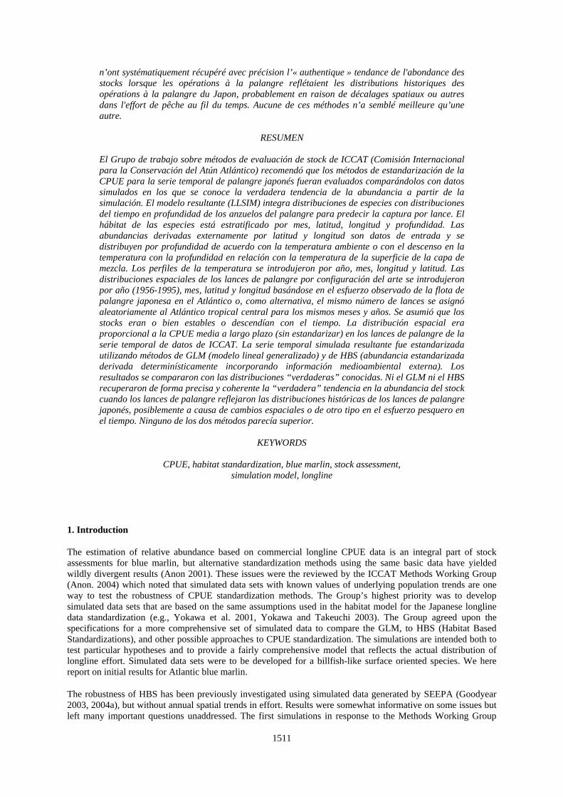
4. Results Relative population trends for the entire Atlantic are illustrated in Figures 4–5 for the true, sampled and resulting CPUE trajectories. The central Atlantic simulation had a larger number of simulated sets (n=559,053) compared to the entire Atlantic (n=242,368) because the sampling rate was increased for the central Atlantic. The entire Atlantic simulation had a higher percentage of zeros (61.2–63.6%) compared to the tropical Atlantic (45.4–47.6%). Model results of the step-wise GLM analysis are provided in Tables 3–4 for the tropical Atlantic and Tables 5–6 for the entire Atlantic. The step-wise inclusion of predictors was the same for the four GLMs. The year effect was initially included due to the necessity of comparing with the groundtruth. The latitude and longitude interaction was included after the year effect and had the largest explanatory ability. The gear effect (HBF) was the 3rd entry in the GLM and the month effect was always the 4th. The percentage of deviance explained ranged from 44.2 to 55.7. Year effects from the GLM and HBS are compared with the groundtruth for the entire Atlantic assuming a stable (Figure 6) and declining population (Figure 7) and the central tropical Atlantic assuming a stable (Figure 8) and declining population (Figure 9). In general, neither the GLM and HBS could reproduce the groundtruth for the entire Atlantic. Both standardization methods did better for the central tropical Atlantic. 5. Discussion The use of a core area in the standardization of BUM CPUE provided better coherence with the groundtruth in the central tropical Atlantic compared to the entire Atlantic. Previous simulations to the entire Atlantic have also demonstrated incoherence between the groundtruth and standardized CPUE series (Takeuchi 2001). The poor results to simulated data were hypothesized to result from a historical shift to higher latitude fishing grounds with a coincident change in the distribution of hooks per basket. While additional simulations are required to rigorously test the inability to reproduce the groundtruth, for stock assessment indices, ICAAT may want to consider BUM standardization of CPUE based on a continuously-fished core area rather than the entire geographical area of fishing when there are substantial annual variations in areas fished among years. The downside of this approach is that it may substantially affect the numbers of samples and areas included in the analyses. The selection of oceanographic variables (e.g. Delta T, ambient temperature, or dissolved oxygen) used in GLMs or habitat-based standardization is a judgment based on knowledge of the species. None of the oceanographic parameters are perfect to vertically distribute a pelagic species, except by chance when a species has relatively little diel variability in habitat. This means that correlations of species affinities to individual environmental variables to be included in the analyses will often be contaminated by diel variations of preferred habitat, e.g., day and nighttime preferred temperatures may be quite different (Goodyear et al. 2008, Hoolihan et al. 2011). On the other hand, temperature and/or dissolved oxygen extremes outside of the tolerance ranges of the species can certainly be used to eliminate unproductive habitat to be excluded from the standardizations and therefore improve the overall robustness of results. It is likely that any one of these variables could be used in the simulations and analyses presented here so long as the simulated environmental affinities or the same for both, but the results might vary. There are additional standardization complications such that a typical tuna longline samples during the entire daytime and a portion of the night and pelagic species have differing diel catchabilities. Habitat based standardizations estimate a composite habitat preference by integrating over the period of longline deployment. An additional complication is if BUM CPUE is high when the longline is deployed or retrieved which cannot be resolved in a GLM framework; however, there is potential to incorporate aspects of longline retrieval in a statHBS approach (Maunder et al. 2006). Additional research could consider:
1) Fit the GLMs to simulated datasets with alternative error distributions, such as Poisson and negative binomial and compare to the lognormal approach with model diagnostics and selection.
2) Conduct an analysis of residuals in a spatial context for the entire Atlantic given the poor performance of both the GLM and HBS.
3) Conduct sensitivity analyses by using alternative gear distributions in a HBS context to evaluate effects on relative abundance estimates.
1514
4) Conduct sensitivity analyses by applying a statHBS (statistical habitat based standardization) with different habitat information as starting parameters to ascertain if the assumed real habitat envelope is reproduced.
Acknowledgements CPG’s contribution to this research was supported by The Billfish Foundation, and KAB’s contribution was supported by the US Department of Commerce, National Marine Fisheries Service. References Anon. 2001, Report of the Fourth ICCAT Billfish Workshop. Collect. Vol. Sci. Pap. ICCAT, 53: 1-130. Anon. 2004, Report of the 2003 meeting of the ICCAT Working Group on Assessment Methods. Collect. Vol.
Sci. Pap. ICCAT, 56(1): 75-105. Goodyear, C. P. 2003, Tests of the robustness of habitat-standardized abundance indices using simulated blue
marlin catch-effort data. Marine and Freshwater Research 2003(54):369-381. Goodyear, C. P. 2004a, SEEPA – a data simulator for testing alternative longline cpue standardization methods.
Collect. Vol. Sci. Pap. ICCAT, 56(1):132-146. Goodyear, C. P. 2004b, Preliminary modifications of SEEPA to conduct simulation studies recommended by the
2003 Meeting of the ICCAT Working Group on Assessment Methods. Collect. Vol. Sci. Pap. ICCAT, 56(1):146-159.
Goodyear, C. P. 2006, Simulated Japanese Longline CPUE for Blue and White Marlin. Collect. Vol. Sci. Pap.
ICCAT, 59(1): 211-223. Goodyear, C. P., Luo, J., Prince, E.D., Hoolihan, J.P., Snodgrass, D., Orbesen, E.S. and Serafy, J.E. 2008,
Vertical habitat use of Atlantic blue marlin Makaira nigricans: interaction with pelagic longline gear. Mar. Eco.l Prog. Ser. 365: 233-245.
Hoolihan, J.P., Luo, J., Goodyear, C.P., Orbesen, E.S. and Prince, E.D. 2011, Vertical habitat use of sailfish
(Istiophorus platypterus) in the Atlantic and eastern Pacific, derived from pop-up satellite archival tag data. Fish. Oceanogr. 20:3, 192-205.
Maunder, M.N., Hinton, M.G., Bigelow, K.A. and Langley, A.D. 2006, Developing indices of abundance using
habitat data in a statistical framework. Bull. Mar. Sci. 79:545-559. Ishii, M. and Kimoto, M. 2009, Reevaluation of historical ocean heat content variations with time-varying xbt
and mbt depth bias corrections. Journal of Oceanography: 65: 287-299. Takeuchi, Y. 2001, Is historically available hooks-per-basket information enough to standardize actual hooks-
Table 3. Selected statistics for the analysis of simulated blue marlin population trends that assumed a tropical Atlantic distribution of the population and fishery and a stable blue marlin population using the GLM as implemented by HBS.
Spatial area: Tropical
Atlantic (CA) Population: Stable
Gear: 5 and 15 hooks between
floats
Sets: 559,053
Null deviance: 496908
Percentage zero catch: 45.4%
Predictor variable
Residual deviance Total d.f. Percent deviance
explained BIC
Year 456266 40 8.2 1473107
Year lat5*lon5 368633 148 25.8 1354311
Year lat5*lon5 HBF
283992 149 42.8 1208482
Year lat5*lon5 HBF Month
277150 160 44.2 1194893
Table 4. Selected statistics for the analysis of simulated blue marlin population trends that assumed a tropical Atlantic distribution of the population and fishery and a stable blue marlin population using the GLM as implemented by HBS.
Spatial area: Tropical
Atlantic (CA)
Population: Decline
Gear: 5 and 15 hooks between
floats
Sets: 559,053
Null deviance: 496550
Percentage zero catch: 47.6%
Predictor variable
Residual deviance Total d.f. Percent deviance
explained BIC
Year 427714 40 13.9 1436981
Year lat5*lon5 347412 148 30.0 1321164
Year lat5*lon5 HBF
277839 149 44.0 1196237
Year lat5*lon5 HBF Month
271513 160 45.3 1183405
1518
Table 5. Selected statistics for the analysis of simulated blue marlin population trends that assumed total Atlantic distribution of the population and fishery and a stable blue marlin population using the GLM as implemented by HBS.
Spatial area: Atlantic (A)
Population: Stable Gear: 5 and 15 hooks between
floats
Sets: 242368
Null deviance: 242368
Percentage zero catch: 63.6%
Predictor variable
Residual deviance Total d.f. Percent deviance
explained BIC
Year 210573 40 24.3 653892
Year lat5*lon5 165251 305 40.6 596218
Year lat5*lon5 HBF
149984 306 47.1 567831
Year lat5*lon5 HBF Month
146242 317 47.4 566648
Table 6. Selected statistics for the analysis of simulated blue marlin population trends that assumed total Atlantic distribution of the population and fishery based on the observed distribution of the Japanese longline effort, ICCAT distributions of CPUE and a declining blue marlin population using the GLM as implemented by HBS.
Spatial area: Atlantic (A)
Population:
Decline
Gear: 5 and 15 hooks between
floats
Sets: 242368 Null deviance:
242368
Percentage zero catch: 61.2%
Predictor variable
Residual deviance Total d.f. Percent deviance
explained BIC
Year 224131 40 34 669016
Year lat5*lon5 117192 305 49.7 604778
Year lat5*lon5 HBF
151067 306 55.5 574471
Year lat5*lon5 HBF Month
150183 317 55.7 573092
1519
Figure 1. Left panel is the Simulator Grid. Right panel is the spatial grid of longline sets when the simulated fishery was constrained to the central Atlantic zone.
Figure 2. Spatial distribution of simulated longline sets for selected years based on the actual distribution of sets by the Japanese longline fishery. Warmer colors indicate larger numbers of sets.
1520
Figure 3. Simulated distribution of longline sets when all sets were constrained to be within the Central Tropical Atlantic zone for all months and years.
Figure 4. True and estimated relative population sizes for a constant population where longline sets matched the spatial distribution of the Japanese fleet in the Atlantic 1956-1995. The simulated fishery started with 5 hooks per basket but shifted to include a large portion of 15 hooks per basket sets after the late 1970s.
1521
Figure 5. True and estimated relative population sizes for a declining population where longline sets matched the spatial distribution of the Japanese fleet in the Atlantic 1956-1995. The simulated fishery started with 5 hooks per basket but shifted to include a large portion of 15 hooks per basket sets after the late 1970s Figure 6. Results of analyses of a simulation assuming constant population (True), using detHBS, and GLM methods. The spatial distribution of the population and fishery covered the entire Atlantic where blue marlin appear in the ICCAT CPUE database (Figures 1 and 2).
Figure 7. Results of analyses of a simulation assuming a declining population (True), using detHBS, and GLM methods. The spatial distribution of the population and fishery covered the entire Atlantic where blue marlin appear in the ICCAT CPUE database (Figures 1 and 2). Figure 8. Results of analyses of a simulation assuming a constant population (True), using detHBS, and GLM methods. The spatial distribution of the population and fishery covered the Central Tropical Atlantic
1523
Figure 9. Results of analyses of a simulation assuming a declining population (True), using detHBS, and GLM methods. The spatial distribution of the population and fishery covered the central tropical Atlantic (Figures 1 and 3).