Page 1
Authors
Christy Ushanth Navaratnam Alf Tørum Øivind A. Arntsen
NT
NU
Norw
eg
ian
Un
ivers
ity o
f Scie
nce
an
d T
echn
olo
gy
Dep
artm
en
t of C
ivil a
nd
Tra
nspo
rt En
gin
ee
ring
R
ep
ort N
o.: IB
AT
/MB
R1
-20
13
PRELIMINARY ANALYSIS OF WAVE SLAMMING FORCE RESPONSE DATA FROM TESTS ON A TRUSS STRUCTURE IN LARGE WAVE FLUME, HANNOVER, GERMANY
29th August 2013, Trondheim, Norway
Page 3
Mail address Ph. +47 73 59 46 40 Location Høgskoleringen 7A Fax +47 73 59 70 21 Høgskoleringen 7A NO-7491 Trondheim Org. no. NO 974 767 880 NORWAY
Norwegian University of
Science and Technology
NTNU Department of Civil and Transport Engineering
REPORT
Title
PRELIMINARY ANALYSIS OF WAVE SLAMMING FORCE
RESPONSE DATA FROM TESTS ON A TRUSS STRUCTURE
IN LARGE WAVE FLUME, HANNOVER, GERMANY
Report no.
BAT/MB-R1/2013.
Date
2013 Authors
Christy Ushanth Navaratnam
Alf Tørum
Øivind A. Arntsen
Sign.
Knut V. Høyland
Head of division ISBN No.
ISBN 978-82-8289-000-7 (Paper Version)
ISBN 978-82-8289-001-4 (Electronic Version)
Number of pages
59
Client
Division of Marine Civil Engineering Availability
Open
Abstract
The foundation of offshore wind turbines are sometimes steel truss structures. In shallow water these
structures may be subjected to wave slamming forces due to plunging breakers. Previous researches show
that the impulsive forces from the plunging wave may be the governing factors in the design response of the
truss structure and the foundations.
Large scale (1:8) tests were carried out at the Large Wave Flume in Hannover Germany in order to
investigate the wave slamming forces on the truss structures and to improve the method to calculate forces
from the plunging breakers. This report presents some of the analysis of the data obtained from the test.
The obtained data were analysed based on total force response as well as the local force response. Total
force data have been analysed using Frequency Response Function (FRF) method whereas the local force
measurements have been analysed using Duhamel integral method as well as the Frequency Response
Function method.
The results showed that the measured slamming forces on the truss is very much less compared to the
calculated slamming forces based on Wienke & Oumeraci (2005). This could be due to the size effects and
wave form when the wave hits the structure. The slamming factor Cs was found to be smaller compared to
the value that was suggested by Wienke & Oumeraci (2005). The pattern of the slamming force distribution
was found to be triangular as found by Sawaragi and Nochino (1984) and Ros (2011). It was found that both
FRF and Duhamel integral methods give almost similar results.
It was found that there is a time phase shift in between the wave profile and the local force measurement
which needs to be investigated and further detailed analyse is recommended in order to come up with better
results.
Stikkord (Norwegian) Keywords (English)
Wave slamming
Response force
Breaking waves
Page 5
i
PREFACE
This report presents some analyses of the data that have been obtained from the experiments on
a truss structure, which was carried out at the Large Wave Channel, Hannover, Germany in May
and June, 2013. The objective of this study to investigate and improve the method to calculate the
wave slamming forces from plunging breaking waves on truss structures through model on a large
scale.
The work described in this publication was supported by the European Community's 7th
Framework Programme through the grant to the budget of the Integrating Activity HYDRALAB
IV, Contract no. 261520.
This document reflects only the authors’ views and not those of the European Community. This
work may rely on data from sources external to the HYDRALAB IV project Consortium.
Members of the Consortium do not accept liability for loss or damage suffered by any third party
as a result of errors or inaccuracies in such data. The information in this document is provided "as
is" and no guarantee or warranty is given that the information is fit for any particular purpose. The
user thereof uses the information at its sole risk and neither the European Community nor any
member of the HYDRALAB IV Consortium is liable for any use that may be made of the
information.
Christy Ushanth Navaratnam
Alf Tørum
Øivind A. Arntsen
NTNU, August 2013
Page 7
ii
TABLE OF CONTENTS
1 INTRODUCTION ........................................................................................................................... 1
2 LITERARURE REVIEW ................................................................................................................ 1
2.1 Morison’s Equation .................................................................................................................... 1
2.2 Wave Slamming Force ............................................................................................................... 2
2.3 Slamming Coefficients ............................................................................................................... 4
2.4 Curling Factor ............................................................................................................................. 5
2.5 Breaking Waves .......................................................................................................................... 6
3 METHODOLGY ............................................................................................................................. 7
3.1 Experimental set-up ................................................................................................................... 7
3.2 Data Analysing Methods ......................................................................................................... 10
3.2.1 Frequency Response Function (FRF) ........................................................................... 11
3.2.2 Duhamel Integral Method .............................................................................................. 12
4 ANALYSIS OF DATA .................................................................................................................. 14
4.1 Total Force Analysis ................................................................................................................ 14
4.1.1 Wave Test ‘2013061424’ with hammer test ‘2406201319’ and ‘Large-hammer-test-
2013_06_24_18_42_58’. ................................................................................................................. 14
4.2 Local Force Transducers ......................................................................................................... 24
4.2.1 Duhamel integral approach: ........................................................................................... 27
4.2.2 FRF Approach .................................................................................................................. 30
5 CONCLUSION AND RECOMMENDATIONS .................................................................... 46
6 REFERENCES ............................................................................................................................... 47
APPENDICES ......................................................................................................................................... 49
Page 8
iii
LIST OF FIGURES
Figure 2.1: Definition sketch of von Karman’s model (Ros Collados, 2011) .................................... 2
Figure 2.2: Definition sketch of impact force on vertical cylinder (Wienke & Oumeraci, 2005) ... 3
Figure 2.3: Definition sketch of 2D impact distribution (Wienke & Oumeraci, 2005) .................... 3
Figure 2.4: Instrumented cylinder [cm]. (Tørum, 2013) ........................................................................ 4
Figure 2.5: Time histories of line forces according to different theories (Wienke & Oumeraci, 2005)
....................................................................................................................................................................... 5
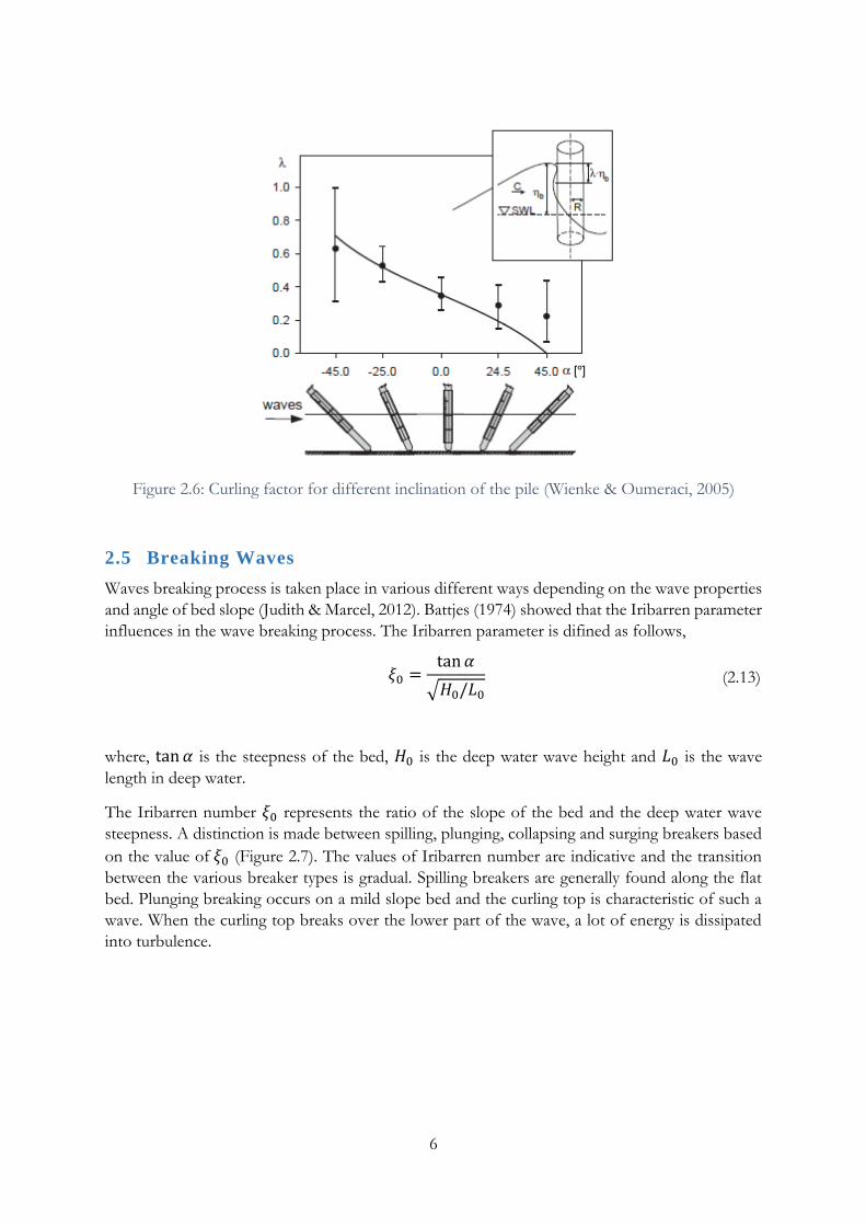
Figure 2.6: Curling factor for different inclination of the pile (Wienke & Oumeraci, 2005) ........... 6
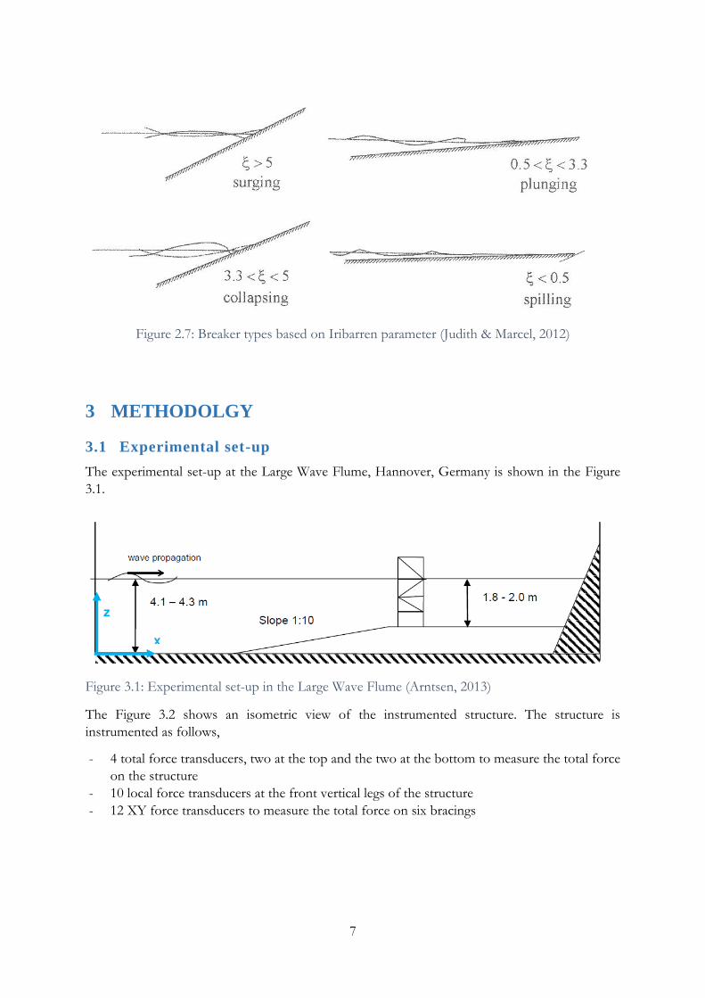
Figure 2.7: Breaker types based on Iribarren parameter (Judith & Marcel, 2012)............................. 7
Figure 3.1: Experimental set-up in the Large Wave Flume (Arntsen, 2013) ...................................... 7
Figure 3.2: Instrumented Structure .......................................................................................................... 8
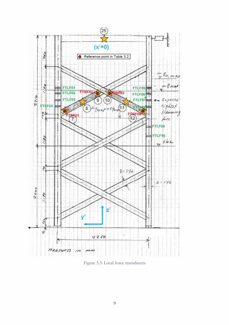
Figure 3.3: Local force transducers .......................................................................................................... 9
Figure 3.4: West side (front). Approximate location of points, marked with big yellow stars, for
application of the 1.5 kg impulse hammer for the whole structure. Approximate location of points,
marked with small yellow stars for application of the 0.1 kg impulse hammer on the local force
cells. (Arntsen, 2013) ................................................................................................................................ 10
Figure 3.5: The derivation of the Duhamel integral (Ros Collados, 2011) ....................................... 12
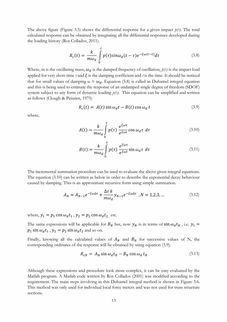
Figure 3.6: Main steps involving in the Duhamel integral approach (Ros Collados, 2011) ........... 14
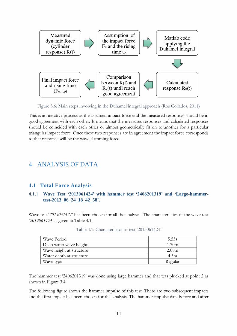
Figure 4.1: Hammer Impulse .................................................................................................................. 15
Figure 4.2: The total response of hammer impulse ............................................................................. 15
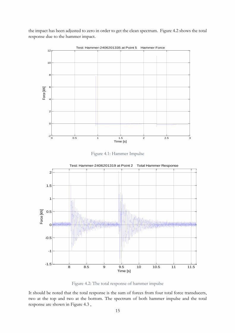
Figure 4.3: Spectrum of hammer and response forces ........................................................................ 16
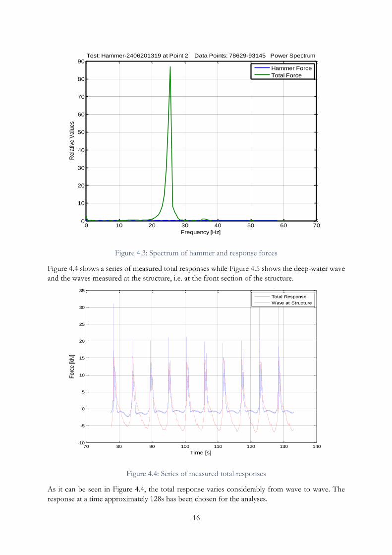
Figure 4.4: Series of measured total responses ..................................................................................... 16
Figure 4.5: Deep water wave and wave at structure [wave period – 5.55s] ...................................... 17
Figure 4.6: Decomposition of total response ....................................................................................... 17
Figure 4.7: Dynamic Response ............................................................................................................... 18
Figure 4.8: Spectrum of dynamic response ........................................................................................... 18
Figure 4.9: Low-pass filtered slamming force variation (with the cut-off frequency of 200Hz) .. 19
Figure 4.10: Hammer impact at point 5. ............................................................................................... 19
Figure 4.11: Total hammer response ...................................................................................................... 20
Figure 4.12: Chosen hammer impulse ................................................................................................... 20
Figure 4.13: Spectrum of the hammer force ......................................................................................... 21
Figure 4.14: Spectrum of both hammer force and total force ........................................................... 21
Figure 4.15: Un-filtered slamming force ................................................................................................ 22
Figure 4.16: Low-pass filtered slamming force (with the cut-off frequency of 200Hz) ................. 22
Figure 4.17: Low-pass filtered slamming force (with the cut-off frequency of 40Hz) ................... 23
Figure 4.18: Hammer impulse and Response on FTLF02 ................................................................. 24
Figure 4.19: Time expanded view of above figure ............................................................................... 25
Figure 4.20: Spectrum of both hammer impulse and the response ................................................... 25
Figure 4.21: Spectrum of the response forces ...................................................................................... 26
Figure 4.22: The maximum response to a suddenly applied triangular force time history (Naess,
..................................................................................................................................................................... 27
Figure 4.23: Duhamel integral approach with impact duration 0.01s and rising time 0.00008s ... 28
Figure 4.24: Duhamel integral approach with impact duration 0.005s and rising time 0.00008s . 28
Figure 4.25: Duhamel integral approach with impact duration 0.005s and rising time 0.0001s ... 29
Figure 4.26: Duhamel integral approach with impact duration 0.005s and rising time 0.0005s ... 29
Figure 4.27: Duhamel integral approach with impact duration 0.005s and rising time 0.0008s ... 30
Figure 4.28: Un-filtered force variation on FTLF02 ........................................................................... 31
Page 9
iv
Figure 4.29: Filtered force variation on FTLF02 [Cut-off frequency- 200Hz] ................................ 31
Figure 4.30: Filtered force variation on FTLF02 [Cut-off frequency- 400Hz] ................................ 32
Figure 4.31: Filtered force variation on FTLF02 [Cut-off frequency- 600Hz] ................................ 32
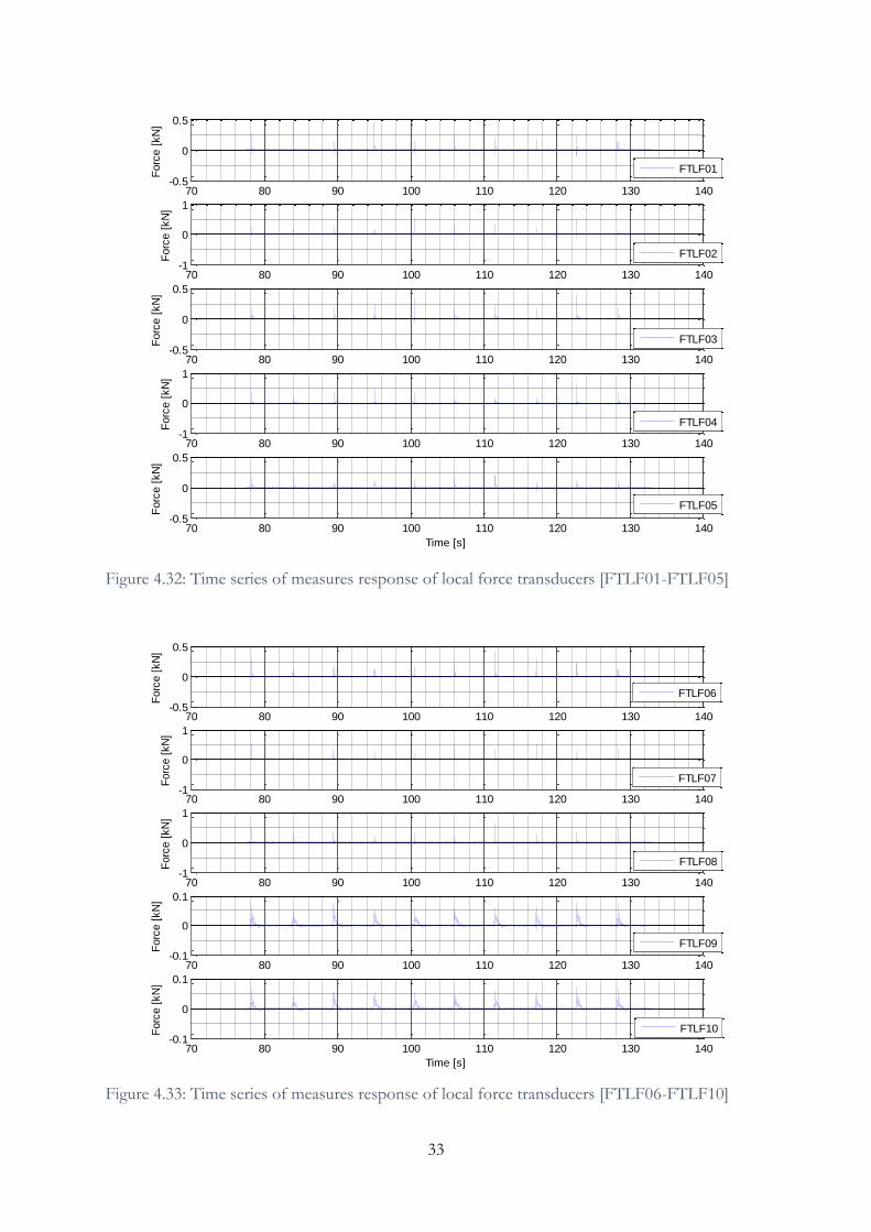
Figure 4.32: Time series of measures response of local force transducers [FTLF01-FTLF05] .... 33
Figure 4.33: Time series of measures response of local force transducers [FTLF06-FTLF10] .... 33
Figure 4.34: Time expanded view of local force transducer responses ............................................ 34
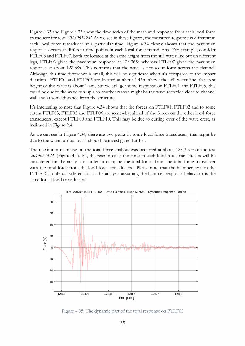
Figure 4.35: The dynamic part of the total response on FTLF02 ..................................................... 35
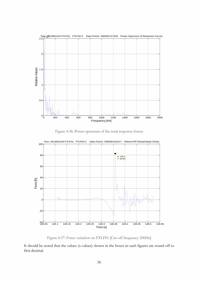
Figure 4.36: Power spectrum of the total response forces ................................................................. 36
Figure 4.37: Force variation on FTLF01 [Cut-off frequency 200Hz] ............................................... 36
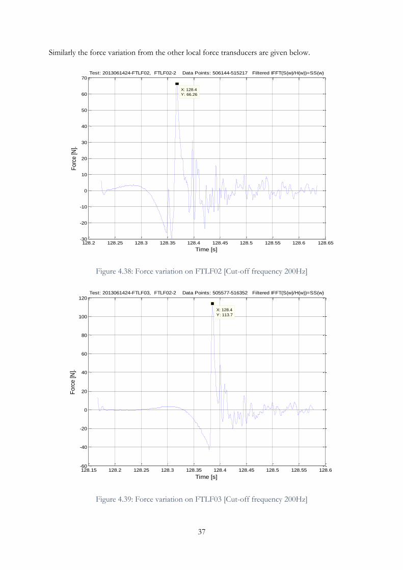
Figure 4.38: Force variation on FTLF02 [Cut-off frequency 200Hz] ............................................... 37
Figure 4.39: Force variation on FTLF03 [Cut-off frequency 200Hz] ............................................... 37
Figure 4.40: Force variation on FTLF04 [Cut-off frequency 200Hz] ............................................... 38
Figure 4.41: Force variation on FTLF05 [Cut-off frequency 200Hz] ............................................... 38
Figure 4.42: Force variation on FTLF06 [Cut-off frequency 200Hz] ............................................... 39
Figure 4.43: Force variation on FTLF07 [Cut-off frequency 200Hz] ............................................... 39
Figure 4.44: Force variation on FTLF08 [Cut-off frequency 200Hz] ............................................... 40
Figure 4.45: Force variation on FTLF09 [Cut-off frequency 200Hz] ............................................... 40
Figure 4.46: Force variation on FTLF10 [Cut-off frequency 200Hz] ............................................... 41
Figure 4.47: The variation of the force intensity with the depth [based on FRF method] at the time
of maximum total response, t=128.3s ................................................................................................... 42
Figure 4.48: Duhamel integral approach for FTLF03 (response at about 128.3s) .......................... 42
Figure 4.49: Duhamel integral approach for FTLF04 (response at about 128.3s) ......................... 43
Figure 4.50: Duhamel integral approach for FTLF07 (response at about 128.3s) .......................... 43
Figure 4.51: Duhamel integral approach for FTLF08 (response at about 128.3s) .......................... 44
Figure 4.52: The variation of the force intensity with the depth [based on Duhamel integral
approach] at the time of maximum total response, t=128.3s ............................................................. 45
Figure 4.53: The response of FTLF02 (blue) and the wave at the structure (red) .......................... 45
Page 10
v
LIST OF TABLES
Table 4.1: Characteristics of test ‘2013061424’ .................................................................................... 14
Table 4.2: Measured forces on each local force transducers [based on FRF method] ................... 41
Table 4.3: Measured forces on each local force transducers [based on Duhamel integral approach]
..................................................................................................................................................................... 44
Page 11
1
1 INTRODUCTION
The foundation of offshore wind turbines are sometimes steel truss structures. In shallow water
these structures may be subjected to wave slamming forces due to plunging breakers. Previous
researches show that the impulsive forces from the plunging wave may be the governing factors
in the design response of the truss structure and the foundations.
Large scale (1:8) tests were carried out at the Large Wave Flume in Hannover Germany in order
to investigate the wave slamming forces on the truss structures and to improve the method to
calculate forces from the plunging breakers. This report presents some of the analysis of the data
obtained from the test.
2 LITERARURE REVIEW
[The following literature review has been directly extracted from the master’s thesis; Navaratnam
(2013)]
Many researches about wave slamming forces or breaking wave forces have been carried out and
still being carried out all over the world. In this chapter, findings from previous researches have
been described.
2.1 Morison’s Equation
The non-breaking wave forces acting on a vertical pile can be calculated using Morison’s equation
(Morison, et al., 1950) which is the summation of the quasi static inertia and drag forces.
𝑑𝐹 = 𝑑𝐹𝐷 + 𝑑𝐹𝑀 =
1
2 𝜌𝑤𝐶𝐷𝐷|𝑢|𝑢 𝑑𝑧 + 𝜌𝑤
𝜋𝐷2
4 𝐶𝑀
𝑑𝑢
𝑑𝑡 𝑑𝑧 (2.1)
Where ρw is the water density, CD is the drag coefficient, CM is the inertia coefficient, D is the
diameter of the pile, u is the water particle velocity, z is the water depth and t is the time. The
values of the drag and coefficients are depending on the Reynolds number, Keulagen Carpenter
number, roughness parameters and interaction parameters (Morison, et al., 1950). The total force
can be obtained by integrating the equation (2.1) along the height of the pile.
𝐹 = 𝐹𝐷 + 𝐹𝑀 = ∫1
2 𝜌𝑤𝐶𝐷𝐷|𝑢|𝑢 𝑑𝑧
𝜂
−𝑑
+ ∫ 𝜌𝑤
𝜋𝐷2
4 𝐶𝑀
𝑑𝑢
𝑑𝑡 𝑑𝑧
𝜂
−𝑑
(2.2)
Where, 𝜂 is the water surface elevation and the d is the total water depth.
The force coefficients CD and CM have been obtained with laboratory experiments. Different range
of values were found for a non-breaking wave for various flow conditions. Generally the Morison
equation is valid for small diameter members that don’t significantly modify the incident waves,
and it depends on the ratio of the wavelength to the member diameter. If this ratio is more than
5, the Morison equation is applicable (Chella, et. al., 2012).
When it comes to breaking wave attack, an additional force of short duration because of the impact
of the vertical breaker front and the breaker tongue has to be considered (Irschik, et. al., 2002).
So, an additional force term which is called ‘slamming force’ (FS) has to be added to the Morison
equation as given in the equation (2.3).
Page 12
2
𝐹 = 𝐹𝐷 + 𝐹𝑀 + 𝐹𝑆 (2.3)
2.2 Wave Slamming Force
The first wave impact model and theoretical formulation of water impact force on rigid body was
derived by von Karman (von Karman, 1929). In his research, he considered a horizontal cylindrical
body with a wedged-shaped under surface as it strikes the horizontal surface of water and
calculated the force acting between the cylindrical body and the water. As it’s shown in the Figure
2.1, a cylinder is approximated by a flat plate of width c(t) which is equal to the immersed portion
of the cylinder at each instant of the impact. The force on this plate could be calculated by
considering the potential flow under the plate and integrating the pressures which can be found
by the Bernoulli’s equation and for this, the time history of the width of the plate should be known
as well.
Figure 2.1: Definition sketch of von Karman’s model (Ros Collados, 2011)
According to von Karman theory, the line force f(t) is given by the following equation,
𝑓(𝑡) = 0.5 𝐶𝑠 𝜌𝑤𝐷 𝐶𝑏2 (2.4)
𝐶𝑠 = 𝜋 (1 −
𝐶𝑏
𝑅𝑡) (2.5)
Where, Cs is the slamming factor, Cb is the wave celerity and D is the diameter of the cylinder and
R is the radius of the cylinder. The maximum line force occurs when the time t is zero (t=0, i.e.
beginning of the impact), and the slamming factor becomes 𝜋.
As this line force is two dimensional and was derived for an infinite length of cylinder based on
von Karman’s model, it should be integrated over the length of the impact area (Figure 2.2) of
cylinder assuming the same line force acting everywhere in the cylinder.
Page 13
3
Figure 2.2: Definition sketch of impact force on vertical cylinder (Wienke & Oumeraci, 2005)
As Figure 2.2 shows, the height of the impact area was found to be the multiplication of the curling
factor λ and the maximum breaking wave crest height ηb (Goda, et. al.,1966). So, the slamming
force Fs on the cylinder,
𝐹𝑠(𝑡) = 0.5 𝜌𝑤𝐷 𝐶𝑏
2 𝜋 (1 −𝐶𝑏
𝑅𝑡) λ 𝜂
𝑏 (2.6)
𝐹𝑠(𝑡) = 𝜋 𝜌𝑤𝑅 𝐶𝑏
2 (1 −𝐶𝑏
𝑅𝑡) λ 𝜂
𝑏 (2.7)
At the beginning of the impact with t=0 the equation (2.7) follows,
𝐹𝑠 = 𝜋 𝜌𝑤𝑅 λ 𝜂𝑏
𝐶𝑏2 (2.8)
From equation (2.4), the line force based on von Karman (1929),
𝑓(𝑡) = 𝜋 𝜌𝑤𝑅 𝐶𝑏2 (2.9)
Figure 2.3: Definition sketch of 2D impact distribution (Wienke & Oumeraci, 2005)
Page 14
4
The line force given in equation (2.9) was obtained by considering the momentum conservation
during the impact. By taking into consideration not only the momentum conservation, but also
the flow beside the flat plate would result in the so-called ‘pile-up effect’, that is the deformation
of the water free surface (Figure 2.3). Because of this pile-up effect, the ‘immersion’ of the cylinder
occurs earlier. As a result, the duration of impact decreases and the maximum line force increases
(Wienke & Oumeraci, 2005).
According to Wagner (1932), the maximum line force is given as follows,
𝑓(𝑡) = 2𝜋 𝜌𝑤𝑅 𝐶𝑏2 (2.10)
The maximum line force calculated by Wagner’s theory is twice the maximum line force calculated
by von Karman’s theory. Generally this maximum line force is described as a function ‘Slamming
Coefficient’ Cs.
𝑓(𝑡) = 𝐶𝑆 𝜌𝑤𝑅 𝐶𝑏2 (2.11)
2.3 Slamming Coefficients
So, the general form of wave slamming force is given in the following equation.
𝐹𝑠 = 𝐶𝑆𝜌𝑤𝑅 λ 𝜂𝑏
𝐶𝑏2 (2.12)
According to von Karman (1929) and Goda et. al. (1966), Cs is π and Wagner’s theory suggests a
Cs value of 2π. Wienke & Oumeraci (2005) suggest a Cs value of 2π as they show that the
formulation of Wagner’s theory is more accurate even though Goda et. al (1966)’s description of
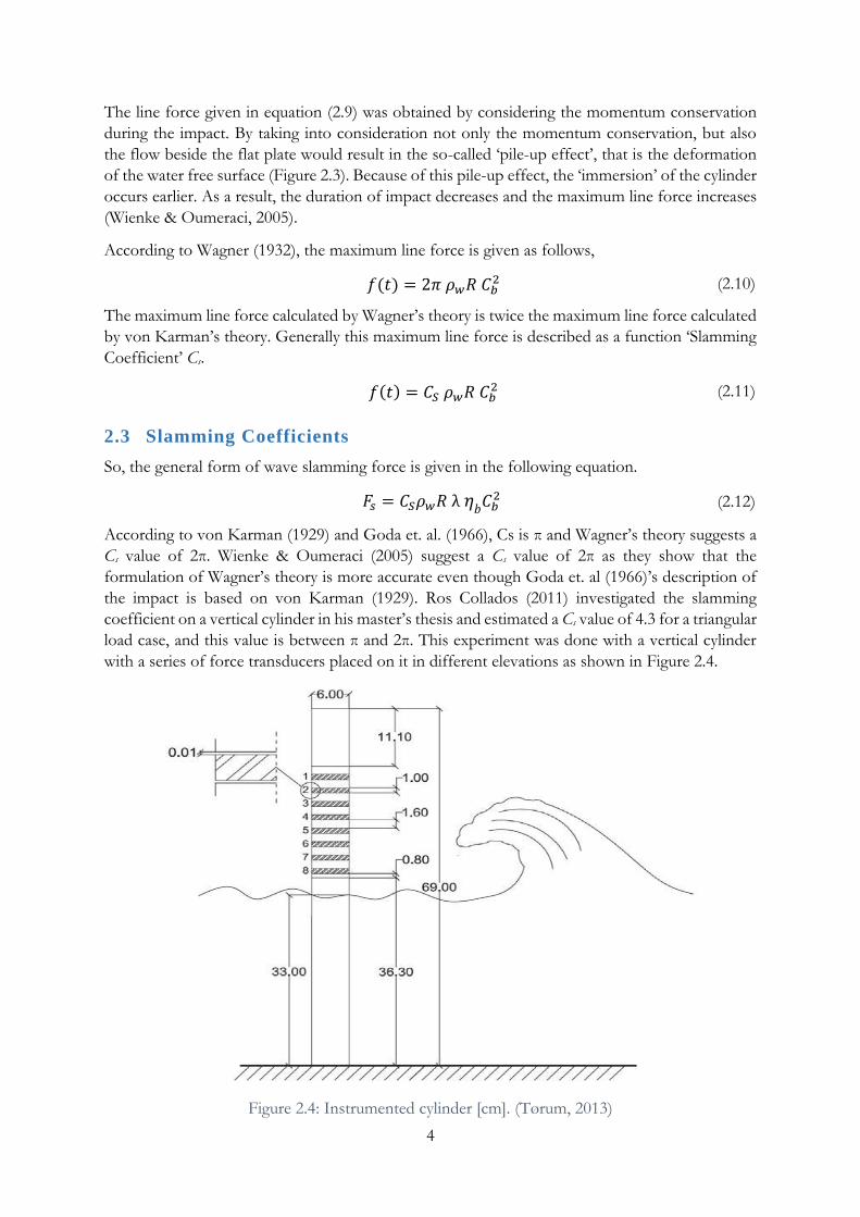
the impact is based on von Karman (1929). Ros Collados (2011) investigated the slamming
coefficient on a vertical cylinder in his master’s thesis and estimated a Cs value of 4.3 for a triangular
load case, and this value is between π and 2π. This experiment was done with a vertical cylinder
with a series of force transducers placed on it in different elevations as shown in Figure 2.4.
Figure 2.4: Instrumented cylinder [cm]. (Tørum, 2013)
Page 15
5
The Cs values were found by considering the maximum impact force at the third transducer. It
should be noted that the impact duration time was set as 0.008s for all the cases, which was defined
at the same time as the triangular load.
Another experiment was carried out by Aune (2011) as part of his master’s thesis and he calculated
a Cs value of 4.77. But, this experiment was performed on a truss structure.
Wienke and Oumeraci (2005) obtained a time history of the impact line force. This is shown in
Figure 2.5. This shows that the value of the line force at the beginning of the impact (t=0), i.e. the
maximum line force that is calculated by their proposed model is equal to the value obtained from
the Wagner’s model.
2.4 Curling Factor
Wienke and Oumeraci (2005) investigated about the curling factor for the vertical and inclined
cylinders. The ratio of the impact force Fs to the line force f(t) provides the height area of the
impact ηb, where ηb is the maximum surface elevation of the breaking wave and the λ is the curling
factor. Figure 2.6 shows the variation of the cylinder factor with the different inclination of the
cylinder, i.e. yaw angle α.
For a vertical cylinder, the maximum curling factor is λ=0.46 and this is in agreement with the
values of curling factors cited in literature, for example, Goda, et. al. (1966) proposed a range of
curling factors λ=0.4-0.5 for plunging wave breakers.
Figure 2.5: Time histories of line forces according to different theories (Wienke & Oumeraci, 2005)
Page 16
6
Figure 2.6: Curling factor for different inclination of the pile (Wienke & Oumeraci, 2005)
2.5 Breaking Waves
Waves breaking process is taken place in various different ways depending on the wave properties
and angle of bed slope (Judith & Marcel, 2012). Battjes (1974) showed that the Iribarren parameter
influences in the wave breaking process. The Iribarren parameter is difined as follows,
𝜉0 =
tan 𝛼
√𝐻0/𝐿0
(2.13)
where, tan 𝛼 is the steepness of the bed, 𝐻0 is the deep water wave height and 𝐿0 is the wave
length in deep water.
The Iribarren number 𝜉0 represents the ratio of the slope of the bed and the deep water wave
steepness. A distinction is made between spilling, plunging, collapsing and surging breakers based
on the value of 𝜉0 (Figure 2.7). The values of Iribarren number are indicative and the transition
between the various breaker types is gradual. Spilling breakers are generally found along the flat
bed. Plunging breaking occurs on a mild slope bed and the curling top is characteristic of such a
wave. When the curling top breaks over the lower part of the wave, a lot of energy is dissipated
into turbulence.
Page 17
7
Figure 2.7: Breaker types based on Iribarren parameter (Judith & Marcel, 2012)
3 METHODOLGY
3.1 Experimental set-up
The experimental set-up at the Large Wave Flume, Hannover, Germany is shown in the Figure
3.1.
Figure 3.1: Experimental set-up in the Large Wave Flume (Arntsen, 2013)
The Figure 3.2 shows an isometric view of the instrumented structure. The structure is
instrumented as follows,
- 4 total force transducers, two at the top and the two at the bottom to measure the total force
on the structure
- 10 local force transducers at the front vertical legs of the structure
- 12 XY force transducers to measure the total force on six bracings
Page 18
8
Figure 3.2: Instrumented Structure
Since there were only forces from total force transducers and the local force transducers were
analysed, the hammer points are shown only for these cases.
Page 19
9
Figure 3.3: Local force transducers
Page 20
10
Figure 3.4: West side (front). Approximate location of points, marked with big yellow stars, for application of the 1.5 kg impulse hammer for the whole structure. Approximate location of points, marked with small yellow stars for application of the 0.1 kg impulse hammer on the local force cells. (Arntsen, 2013)
3.2 Data Analysing Methods
[This section is directly extracted from the master’s thesis; Navaratnam (2013)]
A procedure used by Määtänen (1979) to resolve ice forces from measured response forces on
structures subjected to moving ice is applicable for wave slamming loads as well (Tørum, 2013).
The analysis method that Wienke and Oumeraci (2005) used was deconvolution method which is
similar to Duhamel integral method that was used by Ros Collados (2011). These deconvolution
Page 21
11
and Duhamel integral approaches are more complex for truss structures and have not been used
so far for truss structure. So, the method used by Määtänen (1979), Frequency Response Function
method was used for both individual cylinders and truss structures. But, Duhamel integral method
also used for only individual cylinders in order to compare and check the influence of the analysis
methods.
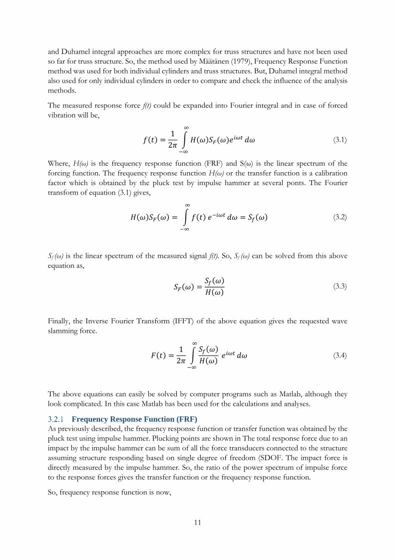
The measured response force f(t) could be expanded into Fourier integral and in case of forced
vibration will be,
𝑓(𝑡) =1
2𝜋∫ 𝐻(𝜔)𝑆𝐹(𝜔)𝑒𝑖𝜔𝑡
∞
−∞
𝑑𝜔 (3.1)
Where, H(ω) is the frequency response function (FRF) and S(ω) is the linear spectrum of the
forcing function. The frequency response function H(ω) or the transfer function is a calibration
factor which is obtained by the pluck test by impulse hammer at several ponts. The Fourier
transform of equation (3.1) gives,
𝐻(𝜔)𝑆𝐹(𝜔) = ∫ 𝑓(𝑡) 𝑒−𝑖𝜔𝑡
∞
−∞
𝑑𝜔 = 𝑆𝑓(𝜔) (3.2)
Sf (ω) is the linear spectrum of the measured signal f(t). So, Sf (ω) can be solved from this above
equation as,
𝑆𝐹(𝜔) =
𝑆𝑓(𝜔)
𝐻(𝜔) (3.3)
Finally, the Inverse Fourier Transform (IFFT) of the above equation gives the requested wave
slamming force.
𝐹(𝑡) =1
2𝜋∫
𝑆𝑓(𝜔)
𝐻(𝜔) 𝑒𝑖𝜔𝑡
∞
−∞
𝑑𝜔 (3.4)
The above equations can easily be solved by computer programs such as Matlab, although they
look complicated. In this case Matlab has been used for the calculations and analyses.
Frequency Response Function (FRF)
As previously described, the frequency response function or transfer function was obtained by the
pluck test using impulse hammer. Plucking points are shown in The total response force due to an
impact by the impulse hammer can be sum of all the force transducers connected to the structure
assuming structure responding based on single degree of freedom (SDOF. The impact force is
directly measured by the impulse hammer. So, the ratio of the power spectrum of impulse force
to the response forces gives the transfer function or the frequency response function.
So, frequency response function is now,
Page 22
12
𝐻(𝜔) =
𝑆𝑇𝑜𝑡𝑎𝑙,ℎ𝑎𝑚𝑚𝑒𝑟(𝜔)
𝑆𝐻𝑎𝑚𝑚𝑒𝑟(𝜔) (3.5)
Where, 𝑆𝑇𝑜𝑡𝑎𝑙,ℎ𝑎𝑚𝑚𝑒𝑟(𝜔) is the fast Fourier transform of the total response forces (power
spectrum) obtained by summing up all the transducer forces due to the impact by the hammer and
𝑆𝐻𝑎𝑚𝑚𝑒𝑟(𝜔) is the fast Fourier transform of the impact measurement obtained directly from
hammer.
𝑆𝑇𝑜𝑡𝑎𝑙,ℎ𝑎𝑚𝑚𝑒𝑟(𝜔) = ∫ 𝑓𝑇𝑜𝑡𝑎𝑙,ℎ𝑎𝑚𝑚𝑒𝑟(𝑡) 𝑒−𝑖𝜔𝑡
∞
−∞
𝑑𝑡 (3.6)
And,
𝑆𝐻𝑎𝑚𝑚𝑒𝑟(𝜔) = ∫ 𝑓𝐻𝑎𝑚𝑚𝑒𝑟(𝑡) 𝑒−𝑖𝜔𝑡
∞
−∞
𝑑𝑡 (3.7)
The frequency response function 𝐻(𝜔) is counter checked by multiplying it by𝑆𝐻𝑎𝑚𝑚𝑒𝑟(𝜔), this
should be equal to𝑆𝑇𝑜𝑡𝑎𝑙,ℎ𝑎𝑚𝑚𝑒𝑟(𝜔). So both the spectrum were checked in order to make sure
it has been done correctly.
Duhamel Integral Method
Duhamel integral approach has been used only for cylinder structures to compare with the results
with the FRF method. The theoretical description of the Duhamel integral method is briefly
described in this chapter. This method was used by Ros Collados (2011) in his master’s thesis.
Figure 3.5: The derivation of the Duhamel integral (Ros Collados, 2011)
Page 23
13
The above figure (Figure 3.5) shows the differential response for a given impact p(τ). The total
calculated response can be obtained by integrating all the differential responses developed during
the loading history (Ros Collados, 2011).
𝑅𝑐(𝑡) = 𝑘
𝑚𝜔𝑑 ∫ 𝑝(𝜏)𝑠𝑖𝑛𝜔𝑑(𝑡 − 𝜏)𝑒−𝜉𝜔(𝑡−𝜏)𝑑𝜏
𝑡
0
(3.8)
Where, m is the oscillating mass, 𝜔𝑑 is the damped frequency of oscillation, p(τ) is the impact load
applied for very short time τ and 𝜉 is the damping coefficient and t is the time. It should be noticed
that for small values of damping ω ≈ 𝜔𝑑. Equation (3.8) is called as Duhamel integral equation
and this is being used to estimate the response of an undamped single degree of freedom (SDOF)
system subject to any form of dynamic loading p(τ). This equation can be simplified and written
as follows (Clough & Penzien, 1975)
𝑅𝑐(𝑡) = 𝐴(𝑡) sin 𝜔𝑑𝑡 − 𝐵(𝑡) cos 𝜔𝑑 𝑡 (3.9)
where,
𝐴(𝑡) =𝑘
𝑚𝜔𝑑∫ 𝑝(𝜏)
𝑒𝜉𝜔𝜏
𝑒𝜉𝜔𝑡cos 𝜔𝑑𝜏 𝑑𝜏
𝑡
0
(3.10)
𝐵(𝑡) =𝑘
𝑚𝜔𝑑∫ 𝑝(𝜏)
𝑒𝜉𝜔𝜏
𝑒𝜉𝜔𝑡sin 𝜔𝑑𝜏 𝑑𝜏
𝑡
0
(3.11)
The incremental summation procedure can be used to evaluate the above given integral equations.
The equation (3.10) can be written as below in order to describe the exponential decay behaviour
caused by damping. This is an approximate recursive form using simple summation.
𝐴𝑁 ≈ 𝐴𝑁−1𝑒−𝜉𝜔∆𝜏 +
∆𝜏 𝑘
𝑚𝜔𝑑𝑦𝑁−1𝑒−𝜉𝜔∆𝜏 , 𝑁 = 1,2,3, … (3.12)
where, 𝑦1 = 𝑝1 cos 𝜔𝑑𝑡1 , 𝑦2 = 𝑝2 cos 𝜔𝑑𝑡2, etc.
The same expressions will be applicable for 𝐵𝑁 but, now 𝑦𝑁 is in terms of sin 𝜔𝑑𝑡𝑁 , i.e. 𝑦1 =
𝑝1 sin 𝜔𝑑𝑡1 , 𝑦2 = 𝑝2 sin 𝜔𝑑𝑡2 and so on.
Finally, knowing all the calculated values of 𝐴𝑁 and 𝐵𝑁 for successive values of N, the
corresponding ordinates of the response will be obtained by using equation (3.9).
𝑅𝑐𝑁 = 𝐴𝑁 sin 𝜔𝑑𝑡𝑁 − 𝐵𝑁 cos 𝜔𝑑 𝑡𝑁 (3.13)
Although these expressions and procedure look more complex, it can be easy evaluated by the
Matlab program. A Matlab code written by Ros Collados (2001) was modified according to the
requirement. The main steps involving in this Duhamel integral method is shown in Figure 3.6.
This method was only used for individual local force meters and was not used for truss structure
sections.
Page 24
14
Figure 3.6: Main steps involving in the Duhamel integral approach (Ros Collados, 2011)
This is an iterative process as the assumed impact force and the measured responses should be in
good agreement with each other. It means that the measures responses and calculated responses
should be coincided with each other or almost geometrically fit on to another for a particular
triangular impact force. Once these two responses are in agreement the impact force corresponds
to that response will be the wave slamming force.
4 ANALYSIS OF DATA
4.1 Total Force Analysis
Wave Test ‘2013061424’ with hammer test ‘2406201319’ and ‘Large-hammer-
test-2013_06_24_18_42_58’.
Wave test ‘2013061424’ has been chosen for all the analyses. The characteristics of the wave test
‘2013061424’ is given in Table 4.1.
Table 4.1: Characteristics of test ‘2013061424’
Wave Period 5.55s
Deep water wave height 1.70m
Wave height at structure 2.08m
Water depth at structure 4.3m
Wave type Regular
The hammer test ‘2406201319’ was done using large hammer and that was plucked at point 2 as
shown in Figure 3.4.
The following figure shows the hammer impulse of this test. There are two subsequent impacts
and the first impact has been chosen for this analysis. The hammer impulse data before and after
Page 25
15
the impact has been adjusted to zero in order to get the clean spectrum. Figure 4.2 shows the total
response due to the hammer impact.
Figure 4.1: Hammer Impulse
Figure 4.2: The total response of hammer impulse
It should be noted that the total response is the sum of forces from four total force transducers,
two at the top and two at the bottom. The spectrum of both hammer impulse and the total
response are shown in Figure 4.3 ,
0 0.5 1 1.5 2 2.5 3-2
0
2
4
6
8
10
12
Time [s]
For
ce [k
N]
Test: Hammer-2406201335 at Point 5 Hammer Force
8 8.5 9 9.5 10 10.5 11 11.5-1.5
-1
-0.5
0
0.5
1
1.5
2
Time [s]
Fo
rce
[kN
]
Test: Hammer-2406201319 at Point 2 Total Hammer Response
Page 26
16
Figure 4.3: Spectrum of hammer and response forces
Figure 4.4 shows a series of measured total responses while Figure 4.5 shows the deep-water wave
and the waves measured at the structure, i.e. at the front section of the structure.
Figure 4.4: Series of measured total responses
As it can be seen in Figure 4.4, the total response varies considerably from wave to wave. The
response at a time approximately 128s has been chosen for the analyses.
0 10 20 30 40 50 60 700
10
20
30
40
50
60
70
80
90
Frequency [Hz]
Re
lativ
e V
alu
es
Test: Hammer-2406201319 at Point 2 Data Points: 78629-93145 Power Spectrum
Hammer Force
Total Force
70 80 90 100 110 120 130 140-10
-5
0
5
10
15
20
25
30
35
Time [s]
Fo
rce
[kN
]
Test: Hammer-2406201335 at Point 5 Total Measured Response
Total Response
Wave at Structure
Page 27
17
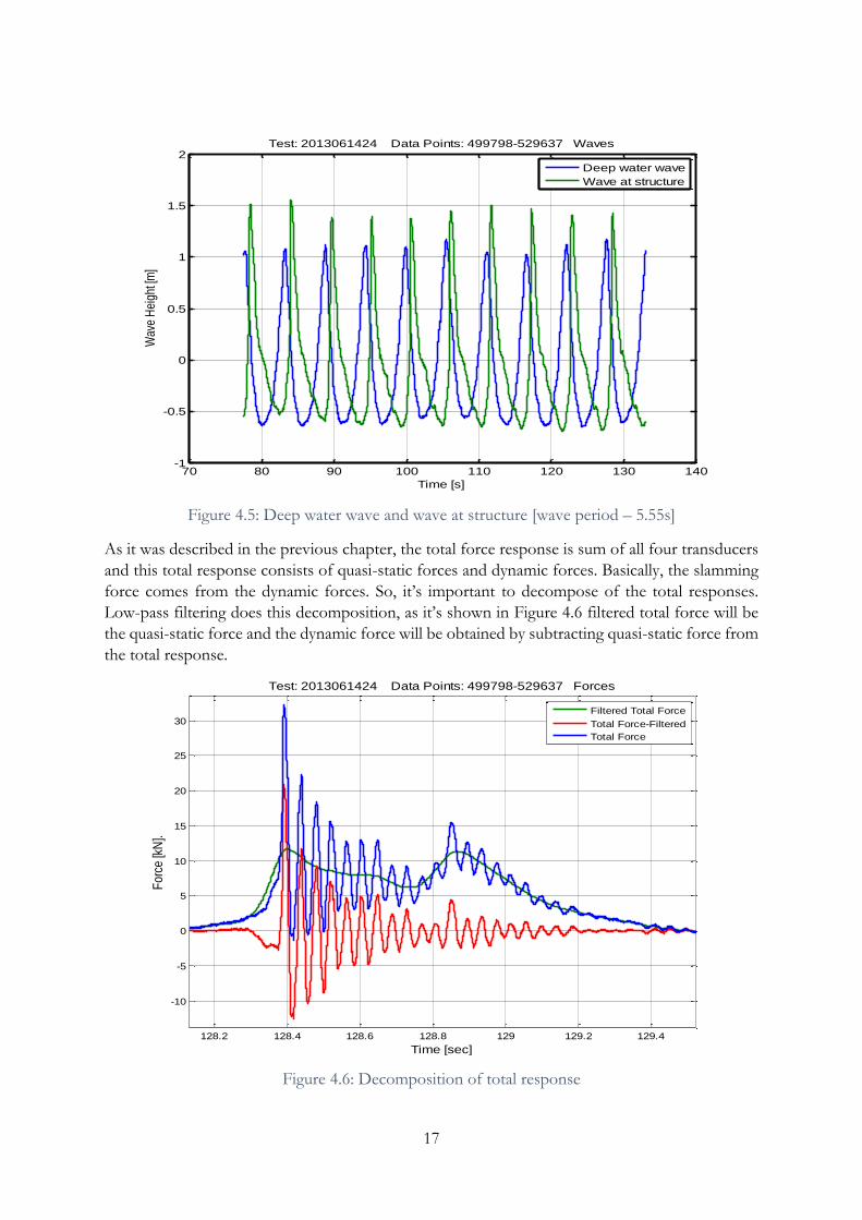
Figure 4.5: Deep water wave and wave at structure [wave period – 5.55s]
As it was described in the previous chapter, the total force response is sum of all four transducers
and this total response consists of quasi-static forces and dynamic forces. Basically, the slamming
force comes from the dynamic forces. So, it’s important to decompose of the total responses.
Low-pass filtering does this decomposition, as it’s shown in Figure 4.6 filtered total force will be
the quasi-static force and the dynamic force will be obtained by subtracting quasi-static force from
the total response.
Figure 4.6: Decomposition of total response
70 80 90 100 110 120 130 140-1
-0.5
0
0.5
1
1.5
2
Time [s]
Wav
e H
eigh
t [m
]Test: 2013061424 Data Points: 499798-529637 Waves
Deep water wave
Wave at structure
128.2 128.4 128.6 128.8 129 129.2 129.4
-10
-5
0
5
10
15
20
25
30
Time [sec]
For
ce [k
N].
Test: 2013061424 Data Points: 499798-529637 Forces
Filtered Total Force
Total Force-Filtered
Total Force
Page 28
18
Figure 4.7: Dynamic Response
Figure 4.8: Spectrum of dynamic response
128.3 128.4 128.5 128.6 128.7 128.8 128.9 129 129.1 129.2 129.3
-10
-5
0
5
10
15
20
25
Time [sec]
Fo
rce
[kN
].
Test: 2013061424 Data Points: 499798-529637 Forces
0 10 20 30 40 50 60 70 0
2000
4000
6000
8000
10000
12000
14000
Frequency [Hz]
Rela
tive V
alu
es
Test: 2013061424, Hammer-2406201319 at Point 2 Data Points: 499798-529637 Power Spectrum of Response Forces
Page 29
19
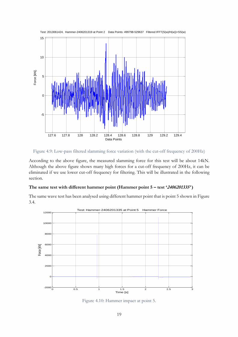
Figure 4.9: Low-pass filtered slamming force variation (with the cut-off frequency of 200Hz)
According to the above figure, the measured slamming force for this test will be about 14kN.
Although the above figure shows many high forces for a cut-off frequency of 200Hz, it can be
eliminated if we use lower cut-off frequency for filtering. This will be illustrated in the following
section.
The same test with different hammer point (Hammer point 5 – test ‘2406201335’ )
The same wave test has been analysed using different hammer point that is point 5 shown in Figure
3.4.
Figure 4.10: Hammer impact at point 5.
0 0.5 1 1.5 2 2.5 3-2000
0
2000
4000
6000
8000
10000
12000
Time [s]
Forc
e [k
N]
Test: Hammer-2406201335 at Point 5 Hammer Force
127.6 127.8 128 128.2 128.4 128.6 128.8 129 129.2 129.4
-5
0
5
10
15
Data Points
Forc
e [kN
].
Test: 2013061424, Hammer-2406201319 at Point 2 Data Points: 499798-529637 Filtered IFFT(S(w)/H(w))=SS(w)
Page 30
20
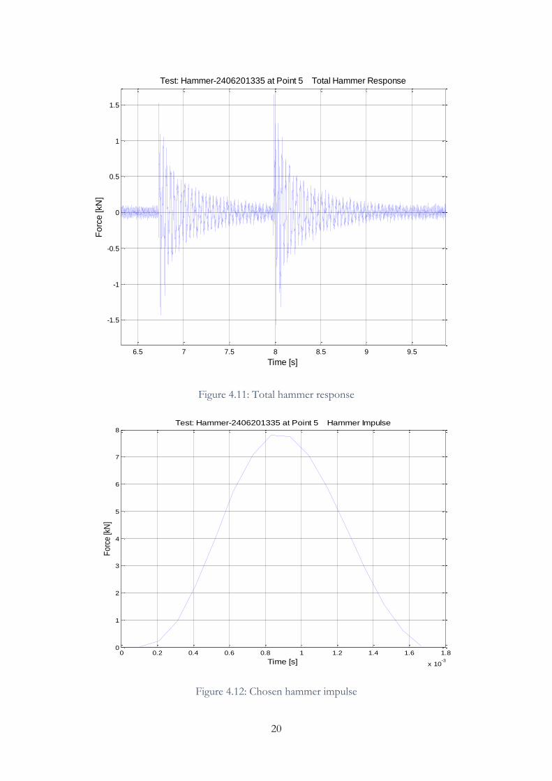
Figure 4.11: Total hammer response
Figure 4.12: Chosen hammer impulse
6.5 7 7.5 8 8.5 9 9.5
-1.5
-1
-0.5
0
0.5
1
1.5
Time [s]
Fo
rce
[kN
]
Test: Hammer-2406201335 at Point 5 Total Hammer Response
0 0.2 0.4 0.6 0.8 1 1.2 1.4 1.6 1.8
x 10-3
0
1
2
3
4
5
6
7
8
Time [s]
Fo
rce
[kN
]
Test: Hammer-2406201335 at Point 5 Hammer Impulse
Page 31
21
Figure 4.13: Spectrum of the hammer force
Figure 4.14: Spectrum of both hammer force and total force
0 10 20 30 40 50 600.205
0.2055
0.206
0.2065
0.207
0.2075
0.208
Frequency [Hz]
Re
lativ
e V
alu
es
Test: Hammer-2406201335 at Point 5 Data Points: 66290-79194 Power Spectrum-Hammer Forces
0 10 20 30 40 50 60 700
20
40
60
80
100
120
Frequency [Hz]
Rel
ativ
e V
alue
s
Test: Hammer-2406201335 at Point 5 Data Points: 66290-79194 Power Spectrum
Hammer Force
Total Force
Page 32
22
Figure 4.15: Un-filtered slamming force
Figure 4.16: Low-pass filtered slamming force (with the cut-off frequency of 200Hz)
127.4 127.6 127.8 128 128.2 128.4 128.6 128.8 129 129.2 129.4 -10
-5
0
5
10
15
Time [s]
Forc
e [kN
].
Test: 2013061424, Hammer-2406201335 at Point 5 Data Points: 499395-536089 IFFT(S(w)/H(w))=SS(w)
127.4 127.6 127.8 128 128.2 128.4 128.6 128.8 129 129.2 129.4 -10
-5
0
5
10
15
Time [s]
Fo
rce [
kN
].
Test: 2013061424, Hammer-2406201335 at Point 5 Data Points: 499395-536089 Filtered IFFT(S(w)/H(w))=SS(w)
Page 33
23
Figure 4.17: Low-pass filtered slamming force (with the cut-off frequency of 40Hz)
According to Figure 4.16 & Figure 4.17, the measured slamming force is approximately 8-13 kN.
Calculated Slamming Force based on Wienke & Oumeraci (2005),
Slamming forces on two front vertical legs = 2 [0.5 ∗ 2𝜋 𝜌𝑤𝐷 λ 𝜂𝑏
𝐶𝑏2]
Wave celerity can be calculated by using the formula, 𝐶𝑏 = √𝑔(ℎ + 𝜂) = √9.81(2 + 1.4)
= 5.77 m/s
So, the slamming forces on two front vertical legs = 2 [0.5*2π*1000*0.14*0.5*1.4*5.772 ]
= 19.99 kN
Length of bracing within the wave impact area = 2 [λ 𝜂𝑏/𝑆𝑖𝑛𝜃]
where, 𝜃 is the inclination of the bracing.
= 2*[0.5*1.4/Sin27.8]
= 3m
Slamming forces on front bracing = 0.5*2π*1000*0.14*3*5.772
= 43.91 kN
So, total slamming force = 63.90 kN
127.4 127.6 127.8 128 128.2 128.4 128.6 128.8 129 129.2 129.4 -4
-2
0
2
4
6
8
10
Time [s]
Fo
rce
[kN
].
Test: 2013061424, Hammer-2406201335 at Point 5 Data Points: 499395-536089 Filtered IFFT(S(w)/H(w))=SS(w)
Page 34
24
As we see from the above calculation, the calculated slamming force based on Wienke & Oumeraci
(2005) is about 64 kN. It should be noted that the calculated slamming force on the bracing is
much more larger than that on two front legs as the length of the bracing that exposed to the
breaking wave is larger.
So, according to the above calculations, the measured slamming force is very less than that we
obtained based on Wienke & Oumeraci (2005).
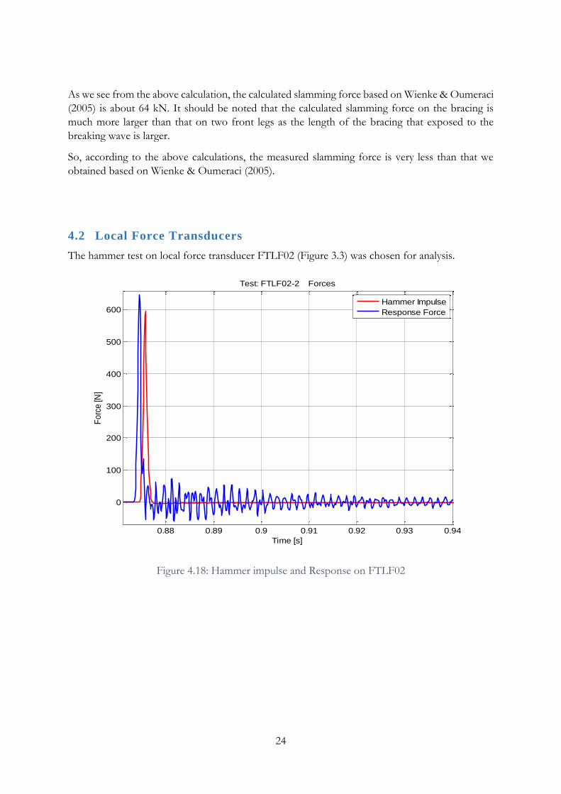
4.2 Local Force Transducers
The hammer test on local force transducer FTLF02 (Figure 3.3) was chosen for analysis.
Figure 4.18: Hammer impulse and Response on FTLF02
0.88 0.89 0.9 0.91 0.92 0.93 0.94
0
100
200
300
400
500
600
Time [s]
Fo
rce
[N]
Test: FTLF02-2 Forces
Hammer Impulse
Response Force
Page 35
25
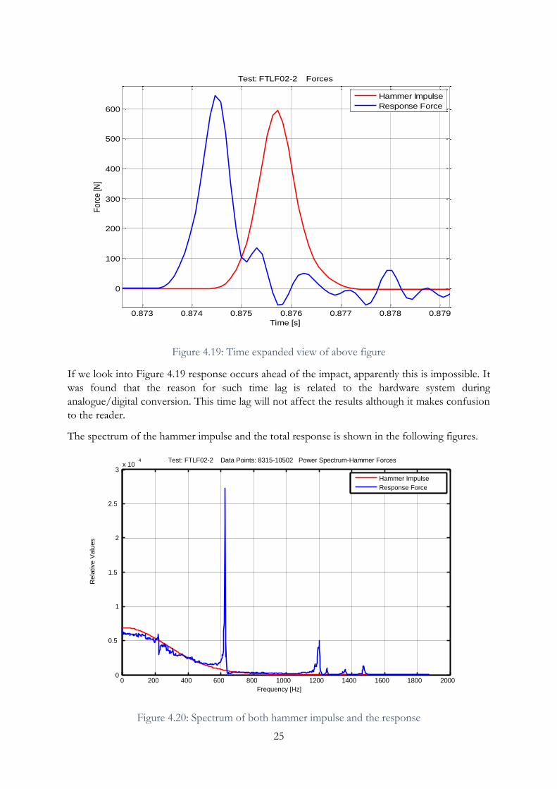
Figure 4.19: Time expanded view of above figure
If we look into Figure 4.19 response occurs ahead of the impact, apparently this is impossible. It
was found that the reason for such time lag is related to the hardware system during
analogue/digital conversion. This time lag will not affect the results although it makes confusion
to the reader.
The spectrum of the hammer impulse and the total response is shown in the following figures.
Figure 4.20: Spectrum of both hammer impulse and the response
0.873 0.874 0.875 0.876 0.877 0.878 0.879
0
100
200
300
400
500
600
Time [s]
Fo
rce
[N]
Test: FTLF02-2 Forces
Hammer Impulse
Response Force
0 200 400 600 800 1000 1200 1400 1600 1800 2000 0
0.5
1
1.5
2
2.5
3 x 10 4
Frequency [Hz]
Re
lative
Va
lue
s
Test: FTLF02-2 Data Points: 8315-10502 Power Spectrum-Hammer Forces
Hammer Impulse Response Force
Page 36
26
Figure 4.21: Spectrum of the response forces
Comments on the spectrum shown in Figure 4.21,
- Decreasing high force until 600Hz due to the clean response signal (similar to the spectrum for
the hammer impulse signal)
- As we see on Figure 4.21, there are two clean peaks at 628 Hz and 1202Hz, this could be due to
the small oscillation in between two peaks in Figure 4.18.
According to Figure 4.19,
The impact duration (td) = 0.0029 s
The natural period of oscillation (tn) = 0.0016s (based on 628Hz)
Ratio td/tn = 1.8125
0 200 400 600 800 1000 1200 1400 1600 1800 2000 0
0.5
1
1.5
2
2.5
3 x 10
4
Frequency [Hz]
Rela
tive V
alu
es
Test: FTLF02-2 Data Points: 8315-10432 Power Spectrum-Response Forces
Page 37
27
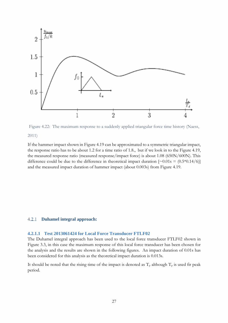
Figure 4.22: The maximum response to a suddenly applied triangular force time history (Naess,
2011)
If the hammer impact shown in Figure 4.19 can be approximated to a symmetric triangular impact,
the response ratio has to be about 1.2 for a time ratio of 1.8., but if we look in to the Figure 4.19,
the measured response ratio (measured response/impact force) is about 1.08 (650N/600N). This
difference could be due to the difference in theoretical impact duration [~0.01s = (0.5*0.14/6)]
and the measured impact duration of hammer impact (about 0.003s) from Figure 4.19.
Duhamel integral approach:
4.2.1.1 Test 2013061424 for Local Force Transducer FTLF02
The Duhamel integral approach has been used to the local force transducer FTLF02 shown in
Figure 3.3, in this case the maximum response of this local force transducer has been chosen for
the analysis and the results are shown in the following figures. An impact duration of 0.01s has
been considered for this analysis as the theoretical impact duration is 0.013s.
It should be noted that the rising time of the impact is denoted as Tp although Tp is used fir peak
period.
Page 38
28
Figure 4.23: Duhamel integral approach with impact duration 0.01s and rising time 0.00008s
When impact duration is 0.005s, the following figure shows the result,
Figure 4.24: Duhamel integral approach with impact duration 0.005s and rising time 0.00008s
0 0.002 0.004 0.006 0.008 0.01 0.012 0.014-100
0
100
200
300
400
500
600
Time [s]
Re
lative
re
sp
on
se
[N
]
Triangular Impulse
Calculated Response
Measured ResponseF0= 303 N
Tp= 0.00008s
0 0.002 0.004 0.006 0.008 0.01 0.012 0.014-100
0
100
200
300
400
500
600
Time [s]
Re
lativ
e r
esp
on
se [N
]
Triangular Impulse
Calculated Response
Measured ResponseF0=315 N
Tp=0.00008s
Page 39
29
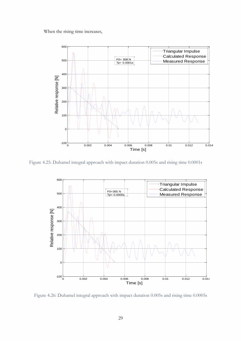
When the rising time increases,
Figure 4.25: Duhamel integral approach with impact duration 0.005s and rising time 0.0001s
Figure 4.26: Duhamel integral approach with impact duration 0.005s and rising time 0.0005s
0 0.002 0.004 0.006 0.008 0.01 0.012 0.014-100
0
100
200
300
400
500
600
Time [s]
Re
lativ
e r
esp
on
se [N
]
Triangular Impulse
Calculated Response
Measured ResponseF0= 308 N
Tp= 0.0001s
0 0.002 0.004 0.006 0.008 0.01 0.012 0.014-100
0
100
200
300
400
500
600
Time [s]
Re
lativ
e r
esp
on
se [N
]
Triangular Impulse
Calculated Response
Measured ResponseF0=365 N
Tp= 0.0005s
Page 40
30
Figure 4.27: Duhamel integral approach with impact duration 0.005s and rising time 0.0008s
4.2.1.2 Measured Slamming Factor
As we see in the above figures, when the rising time increases, the impact force also increases and
finally it becomes very hard to fit the measured response curve as it lags behind it.
According to Figure 4.23, the measured Cs value will be,
Measured slamming factor [Cs] = Fs/[0.5 𝜌𝑤𝐷 ℎ 𝐶𝑏2]
= 303/ [0.5*1000*0.14*0.04*5.772]
= 3.33
As we see from the above calculation, the slamming factor is very small compared to the slamming
factor 2π that Wienke & Oumeraci (2005) used.
Since the maximum total response occurred at the FTLF02 and the measured slamming force also
found to be highest compared to the slamming force that has been obtained from the other local
force transducers (Figure 4.32 & Figure 4.33 ), the above slamming factor will be larger than the
slamming factor that can be obtained from other local forces
FRF Approach
Now we consider the Frequency Response Function method for the same local force transducer
FTLF02. Hammer tests that were done on FTLF02 has been used in all the analysis in order to
compare the results of both the analysing methods, Duhamel integral approach and frequency
response function method.
0 0.002 0.004 0.006 0.008 0.01 0.012 0.0140
100
200
300
400
500
600
Time [s]
Re
lative
re
sp
on
se
[N
]
Triangular Impulse
Calculated Response
Measured ResponseTp=0.0008s
Page 41
31
Figure 4.28: Un-filtered force variation on FTLF02
Figure 4.29: Filtered force variation on FTLF02 [Cut-off frequency- 200Hz]
100.35 100.4 100.45 100.5 100.55 100.6 100.65 100.7 100.75 100.8 100.85-600
-400
-200
0
200
400
600
800
Time [s]
Fo
rce
[N].
Test: 2013061424-FTLF02, FTLF02-2 Data Points: 227694-237335 IFFT(S(w)/H(w))=SS(w)
100.35 100.4 100.45 100.5 100.55 100.6 100.65 100.7 100.75 100.8 100.85-50
0
50
100
150
200
Time [s]
Fo
rce
[N
].
Test: 2013061424-FTLF02, FTLF02-2 Data Points: 227694-237335 Filtered IFFT(S(w)/H(w))=SS(w)
Page 42
32
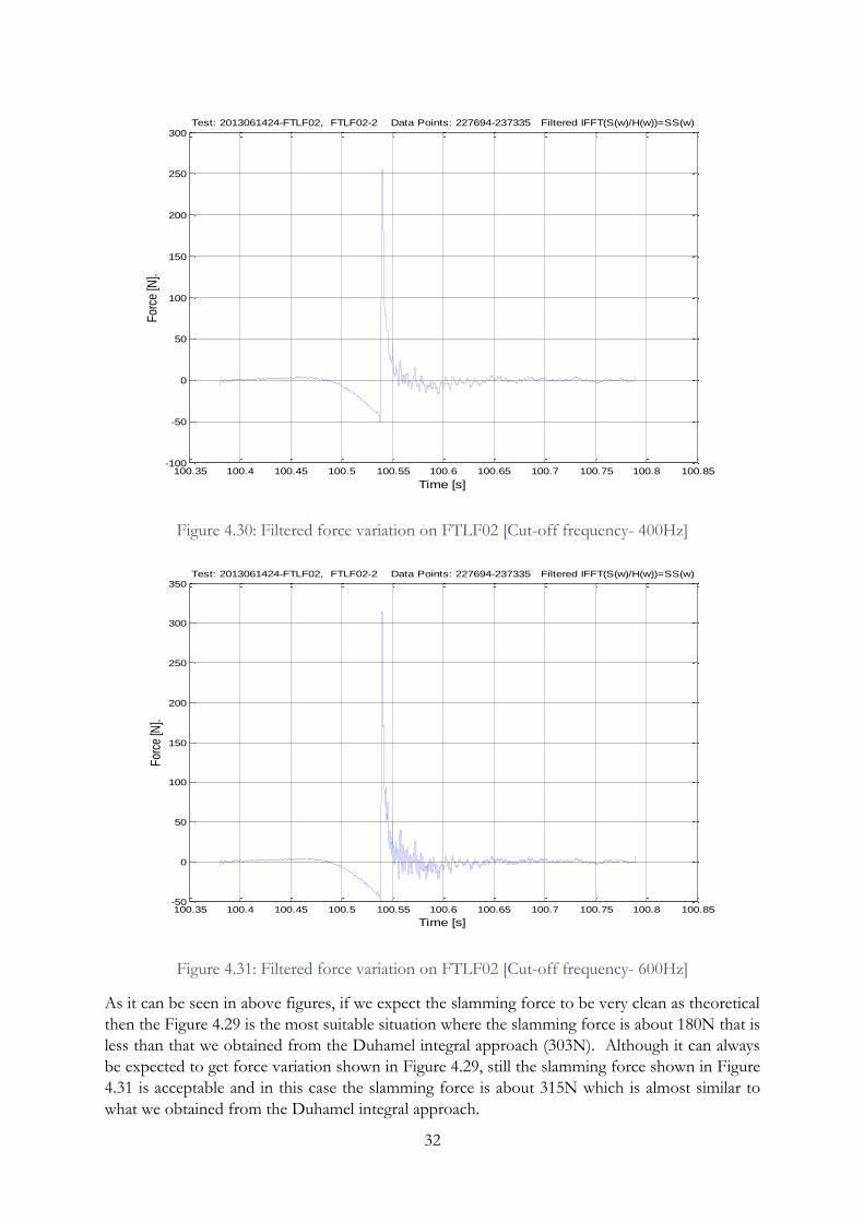
Figure 4.30: Filtered force variation on FTLF02 [Cut-off frequency- 400Hz]
Figure 4.31: Filtered force variation on FTLF02 [Cut-off frequency- 600Hz]
As it can be seen in above figures, if we expect the slamming force to be very clean as theoretical
then the Figure 4.29 is the most suitable situation where the slamming force is about 180N that is
less than that we obtained from the Duhamel integral approach (303N). Although it can always
be expected to get force variation shown in Figure 4.29, still the slamming force shown in Figure
4.31 is acceptable and in this case the slamming force is about 315N which is almost similar to
what we obtained from the Duhamel integral approach.
100.35 100.4 100.45 100.5 100.55 100.6 100.65 100.7 100.75 100.8 100.85-100
-50
0
50
100
150
200
250
300
Time [s]
For
ce [N
].
Test: 2013061424-FTLF02, FTLF02-2 Data Points: 227694-237335 Filtered IFFT(S(w)/H(w))=SS(w)
100.35 100.4 100.45 100.5 100.55 100.6 100.65 100.7 100.75 100.8 100.85-50
0
50
100
150
200
250
300
350
Time [s]
For
ce [N
].
Test: 2013061424-FTLF02, FTLF02-2 Data Points: 227694-237335 Filtered IFFT(S(w)/H(w))=SS(w)
Page 43
33
Figure 4.32: Time series of measures response of local force transducers [FTLF01-FTLF05]
Figure 4.33: Time series of measures response of local force transducers [FTLF06-FTLF10]
70 80 90 100 110 120 130 140-0.5
0
0.5
Forc
e [
kN
]
FTLF01
70 80 90 100 110 120 130 140-1
0
1
Forc
e [
kN
]
FTLF02
70 80 90 100 110 120 130 140-0.5
0
0.5
Forc
e [
kN
]
FTLF03
70 80 90 100 110 120 130 140-1
0
1
Forc
e [
kN
]
FTLF04
70 80 90 100 110 120 130 140-0.5
0
0.5
Time [s]
Forc
e [
kN
]
FTLF05
70 80 90 100 110 120 130 140-0.5
0
0.5
Forc
e [
kN
]
FTLF06
70 80 90 100 110 120 130 140-1
0
1
Forc
e [
kN
]
FTLF07
70 80 90 100 110 120 130 140-1
0
1
Forc
e [
kN
]
FTLF08
70 80 90 100 110 120 130 140-0.1
0
0.1
Forc
e [
kN
]
FTLF09
70 80 90 100 110 120 130 140-0.1
0
0.1
Time [s]
Forc
e [
kN
]
FTLF10
Page 44
34
Figure 4.34: Time expanded view of local force transducer responses
128.1 128.2 128.3 128.4 128.5 128.6 128.7-0.2
0
0.2
Time [s]
Forc
e [
kN
]
FTLF01
128.1 128.2 128.3 128.4 128.5 128.6 128.7-0.2
0
0.2
Time [s]
Forc
e [
kN
]
FTLF02
128.1 128.2 128.3 128.4 128.5 128.6 128.7-0.2
0
0.2
Time [s]
Forc
e [
kN
]
FTLF03
128.1 128.2 128.3 128.4 128.5 128.6 128.7-0.5
0
0.5
Time [s]
Forc
e [
kN
]
FTLF04
128.1 128.2 128.3 128.4 128.5 128.6 128.7-0.2
0
0.2
Time [s]
Forc
e [
kN
]
FTLF05
128.1 128.2 128.3 128.4 128.5 128.6 128.7-0.2
0
0.2
Time [s]
Forc
e [
kN
]
FTLF06
128.1 128.2 128.3 128.4 128.5 128.6 128.7-0.5
0
0.5
Time [s]
Forc
e [
kN
]
FTLF07
128.1 128.2 128.3 128.4 128.5 128.6 128.7-0.5
0
0.5
Time [s]
Forc
e [
kN
]
FTLF08
128.1 128.2 128.3 128.4 128.5 128.6 128.7-0.1
0
0.1
Time [s]
Forc
e [
kN
]
FTLF09
128.1 128.2 128.3 128.4 128.5 128.6 128.7-0.1
0
0.1
Time [s]
Forc
e [
kN
]
FTLF10
Page 45
35
Figure 4.32 and Figure 4.33 show the time series of the measured response from each local force
transducer for test ‘2013061424’. As we see in these figures, the measured response is different in
each local force transducer at a particular time. Figure 4.34 clearly shows that the maximum
response occurs at different time points in each local force transducers. For example, consider
FTLF03 and FTLF07, both are located at the same height from the still water line but on different
legs, FTLF03 gives the maximum response at 128.365s whereas FTLF07 gives the maximum
response at about 128.38s. This confirms that the wave is not so uniform across the channel.
Although this time difference is small, this will be significant when it’s compared to the impact
duration. FTLF01 and FTLF05 are located at about 1.45m above the still water line, the crest
height of this wave is about 1.4m, but we still get some response on FTLF01 and FTLF05, this
could be due to the wave run-up also another reason might be the wave recorded close to channel
wall and at some distance from the structure.
It’s interesting to note that Figure 4.34 shows that the forces on FTLF01, FTLF02 and to some
extent FTLF03, FTLF05 and FTLF06 are somewhat ahead of the forces on the other local force
transducers, except FTLF09 and FTLF10. This may be due to curling over of the wave crest, as
indicated in Figure 2.4.
As we can see in Figure 4.34, there are two peaks in some local force transducers, this might be
due to the wave run-up, but it should be investigated further.
The maximum response on the total force analysis was occurred at about 128.3 sec of the test
‘2013061424’ (Figure 4.4). So, the responses at this time in each local force transducers will be
considered for the analysis in order to compare the total forces from the total force transducer
with the total force from the local force transducers. Please note that the hammer test on the
FTLF02 is only considered for all the analysis assuming the hammer response behaviour is the
same for all local transducers.
Figure 4.35: The dynamic part of the total response on FTLF02
128.3 128.4 128.5 128.6 128.7 128.8
-60
-40
-20
0
20
40
60
80
Time [sec]
Fo
rce
[N].
Test: 2013061424-FTLF02 Data Points: 505847-517540 Dynamic Response Forces
Page 46
36
Figure 4.36: Power spectrum of the total response forces
Figure 4.37: Force variation on FTLF01 [Cut-off frequency 200Hz]
It should be noted that the values (x-values) shown in the boxes in each figures are round off to
first decimal.
0 200 400 600 800 1000 1200 1400 1600 1800 20000
0.5
1
1.5
2
2.5x 10
4
Frequency [Hz]
Re
lativ
e V
alu
es
Test: 2013061424-FTLF01, FTLF02-2 Data Points: 506250-517944 Power Spectrum of Response Forces
128.05 128.1 128.15 128.2 128.25 128.3 128.35 128.4 128.45 128.5 128.55-40
-20
0
20
40
60
80
100
X: 128.4
Y: 82.89
Time [s]
Fo
rce
[N].
Test: 2013061424-FTLF01, FTLF02-2 Data Points: 505009-515217 Filtered IFFT(S(w)/H(w))=SS(w)
Page 47
37
Similarly the force variation from the other local force transducers are given below.
Figure 4.38: Force variation on FTLF02 [Cut-off frequency 200Hz]
Figure 4.39: Force variation on FTLF03 [Cut-off frequency 200Hz]
128.2 128.25 128.3 128.35 128.4 128.45 128.5 128.55 128.6 128.65-30
-20
-10
0
10
20
30
40
50
60
70
X: 128.4
Y: 66.26
Time [s]
Fo
rce
[N].
Test: 2013061424-FTLF02, FTLF02-2 Data Points: 506144-515217 Filtered IFFT(S(w)/H(w))=SS(w)
128.15 128.2 128.25 128.3 128.35 128.4 128.45 128.5 128.55 128.6-60
-40
-20
0
20
40
60
80
100
120
X: 128.4
Y: 113.7
Time [s]
Fo
rce
[N].
Test: 2013061424-FTLF03, FTLF02-2 Data Points: 505577-516352 Filtered IFFT(S(w)/H(w))=SS(w)
Page 48
38
Figure 4.40: Force variation on FTLF04 [Cut-off frequency 200Hz]
Figure 4.41: Force variation on FTLF05 [Cut-off frequency 200Hz]
128.15 128.2 128.25 128.3 128.35 128.4 128.45 128.5 128.55 128.6-50
0
50
100
150
X: 128.4
Y: 144.4
Time [s]
Fo
rce
[N].
Test: 2013061424-FTLF04, FTLF02-2 Data Points: 505577-519187 Filtered IFFT(S(w)/H(w))=SS(w)
128.2 128.25 128.3 128.35 128.4 128.45 128.5 128.55 128.6 128.65-30
-20
-10
0
10
20
30
40
50
60
X: 128.4
Y: 50.03
Time [s]
Fo
rce
[N].
Test: 2013061424-FTLF05, FTLF02-2 Data Points: 506144-514650 Filtered IFFT(S(w)/H(w))=SS(w)
Page 49
39
Figure 4.42: Force variation on FTLF06 [Cut-off frequency 200Hz]
Figure 4.43: Force variation on FTLF07 [Cut-off frequency 200Hz]
128.15 128.2 128.25 128.3 128.35 128.4 128.45 128.5 128.55 128.6-30
-20
-10
0
10
20
30
40
50X: 128.4
Y: 42.78
Time [s]
For
ce [N
].
Test: 2013061424-FTLF06, FTLF02-2 Data Points: 505577-514083 Filtered IFFT(S(w)/H(w))=SS(w)
X: 128.4
Y: 37.96
128.2 128.25 128.3 128.35 128.4 128.45 128.5 128.55 128.6 128.65-50
0
50
100
150
200
X: 128.4
Y: 164.9
Time [s]
Fo
rce
[N].
Test: 2013061424-FTLF07, FTLF02-2 Data Points: 506144-517486 Filtered IFFT(S(w)/H(w))=SS(w)
Page 50
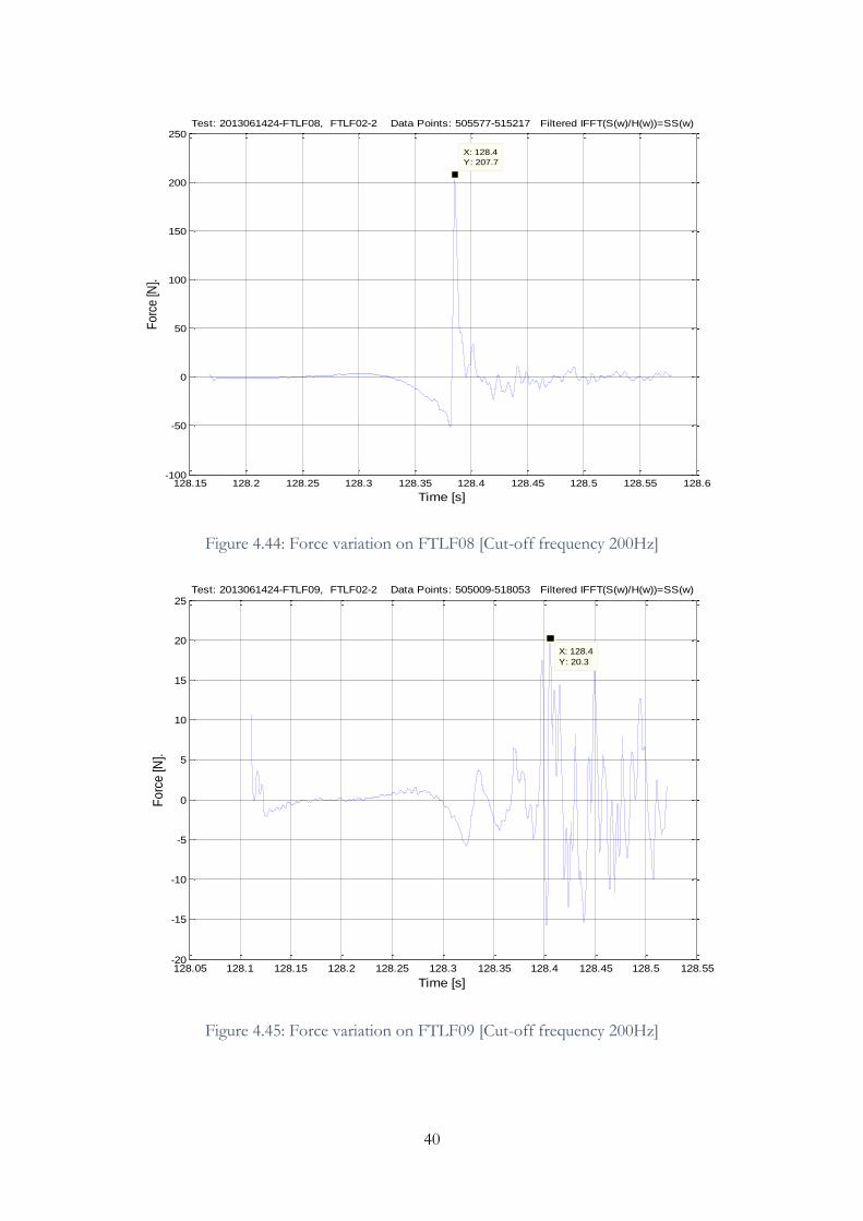
40
Figure 4.44: Force variation on FTLF08 [Cut-off frequency 200Hz]
Figure 4.45: Force variation on FTLF09 [Cut-off frequency 200Hz]
128.15 128.2 128.25 128.3 128.35 128.4 128.45 128.5 128.55 128.6-100
-50
0
50
100
150
200
250
X: 128.4
Y: 207.7
Time [s]
Fo
rce
[N].
Test: 2013061424-FTLF08, FTLF02-2 Data Points: 505577-515217 Filtered IFFT(S(w)/H(w))=SS(w)
128.05 128.1 128.15 128.2 128.25 128.3 128.35 128.4 128.45 128.5 128.55-20
-15
-10
-5
0
5
10
15
20
25
X: 128.4
Y: 20.3
Time [s]
Fo
rce
[N].
Test: 2013061424-FTLF09, FTLF02-2 Data Points: 505009-518053 Filtered IFFT(S(w)/H(w))=SS(w)
Page 51
41
Figure 4.46: Force variation on FTLF10 [Cut-off frequency 200Hz]
As it can be seen in all the above figures, the maximum force occurred at around 128.355s and the
local force transducers FTLF09 and FTLF10 give very less or almost no force at this time as its
located away from the slamming point. The following table shows the summary of the forces of
each transducers. Please note that the z is the height above the still water line, which means that z
is zero at the still water line.
Table 4.2: Measured forces on each local force transducers [based on FRF method]
FTLF Z (mm) Meas. Force
(N)
Front Leg 1 1 1450 82.89
2 1300 66.26
3 1150 113.7
4 1063 144.4 407.25
Front Leg 2 5 1450 50.03
6 1300 37.96
7 1150 164.9
8 1063 207.7
9 377 20.3
10 250 20.3 501.19
908.44
128.05 128.1 128.15 128.2 128.25 128.3 128.35 128.4 128.45 128.5 128.55-20
-15
-10
-5
0
5
10
15
20
25
X: 128.4
Y: 20.33
Time [s]
Fo
rce
[N].
Test: 2013061424-FTLF10, FTLF02-2 Data Points: 505009-519187 Filtered IFFT(S(w)/H(w))=SS(w)
Page 52
42
Based on the above table, the force intensity has been plotted against the location each transducers
which is shown in the following figure.
Figure 4.47: The variation of the force intensity with the depth [based on FRF method] at the time of maximum total response, t=128.3s
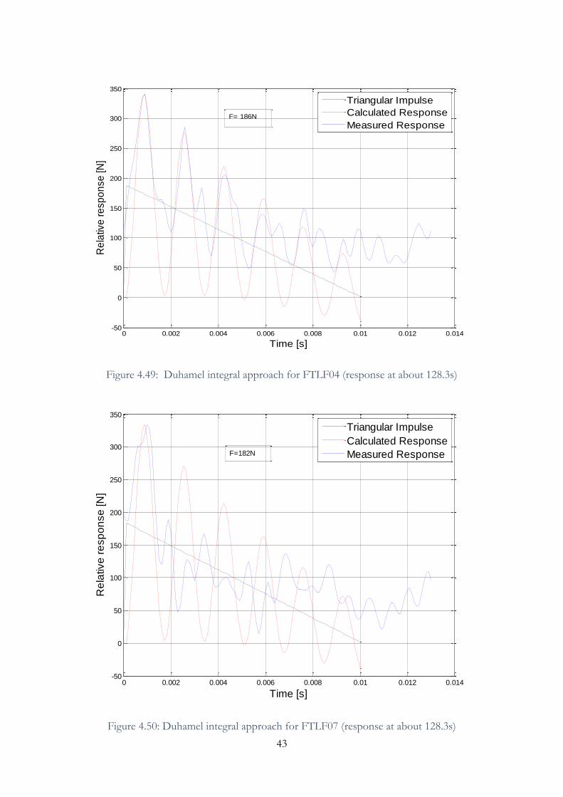
The response from all individual local force transducers at 128.3s has been analysed using Duhamel
integral approach. Few of them (those give maximum forces) shown in the following figures.
Figure 4.48: Duhamel integral approach for FTLF03 (response at about 128.3s)
0
200
400
600
800
1000
1200
1400
1600
0 1 2 3 4 5 6
Z [m
m]
fs [N/mm]
Front Leg 1
Front Leg 2
0 0.002 0.004 0.006 0.008 0.01 0.012 0.014-50
0
50
100
150
200
Time [s]
Re
lativ
e r
esp
on
se [N
]
Triangular Impulse
Calculated Response
Measured ResponseF=99 N
Page 53
43
Figure 4.49: Duhamel integral approach for FTLF04 (response at about 128.3s)
Figure 4.50: Duhamel integral approach for FTLF07 (response at about 128.3s)
0 0.002 0.004 0.006 0.008 0.01 0.012 0.014-50
0
50
100
150
200
250
300
350
Time [s]
Re
lativ
e r
esp
on
se
[N
]
Triangular Impulse
Calculated Response
Measured ResponseF= 186N
0 0.002 0.004 0.006 0.008 0.01 0.012 0.014-50
0
50
100
150
200
250
300
350
Time [s]
Re
lative
re
sp
on
se
[N
]
Triangular Impulse
Calculated Response
Measured ResponseF=182N
Page 54
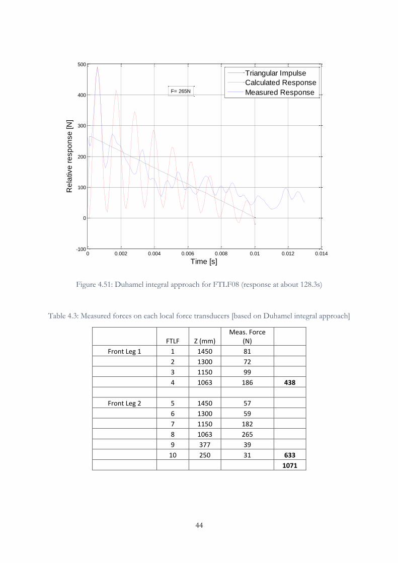
44
Figure 4.51: Duhamel integral approach for FTLF08 (response at about 128.3s)
Table 4.3: Measured forces on each local force transducers [based on Duhamel integral approach]
FTLF Z (mm) Meas. Force
(N)
Front Leg 1 1 1450 81
2 1300 72
3 1150 99
4 1063 186 438
Front Leg 2 5 1450 57
6 1300 59
7 1150 182
8 1063 265
9 377 39
10 250 31 633
1071
0 0.002 0.004 0.006 0.008 0.01 0.012 0.014-100
0
100
200
300
400
500
Time [s]
Re
lative
re
sp
on
se
[N
]
Triangular Impulse
Calculated Response
Measured ResponseF= 265N
Page 55
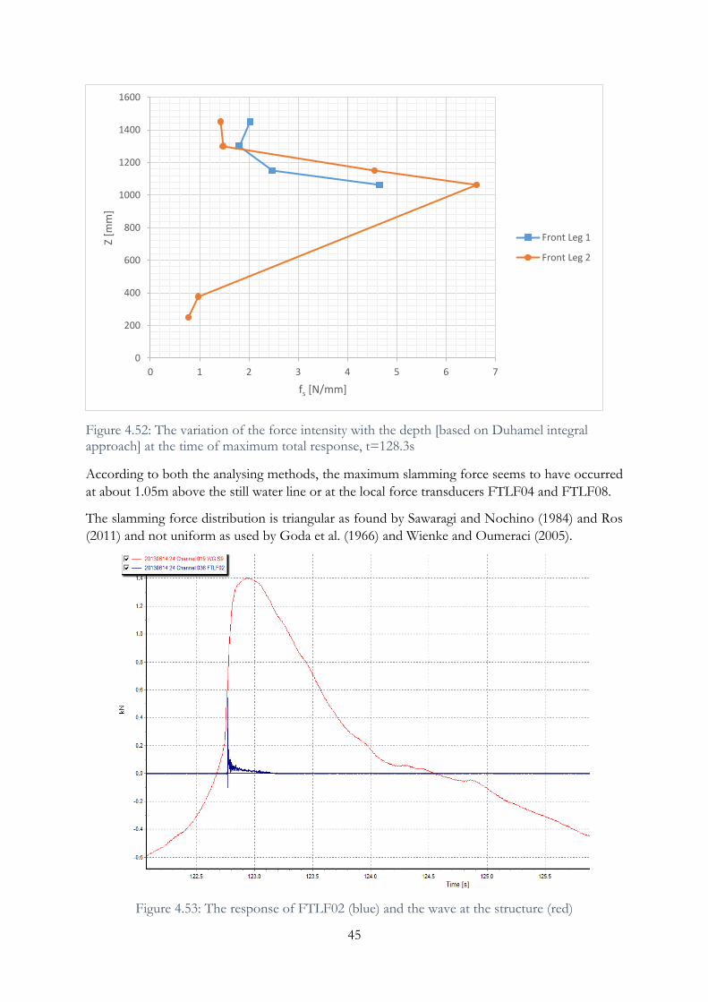
45
Figure 4.52: The variation of the force intensity with the depth [based on Duhamel integral approach] at the time of maximum total response, t=128.3s
According to both the analysing methods, the maximum slamming force seems to have occurred
at about 1.05m above the still water line or at the local force transducers FTLF04 and FTLF08.
The slamming force distribution is triangular as found by Sawaragi and Nochino (1984) and Ros
(2011) and not uniform as used by Goda et al. (1966) and Wienke and Oumeraci (2005).
Figure 4.53: The response of FTLF02 (blue) and the wave at the structure (red)
0
200
400
600
800
1000
1200
1400
1600
0 1 2 3 4 5 6 7
Z [m
m]
fs [N/mm]
Front Leg 1
Front Leg 2
Page 56
46
As we see in Figure 4.53, the maximum wave crest occurs at about 122.9s and the maximum
response occurs at 122.75s, this indicates that there is a time phase shift which is still unclear and
needs to be investigated further.
5 CONCLUSION AND RECOMMENDATIONS
There were few data analysed and presented in this report. Initially the total force on the structure
was analysed using Frequency Response Function (FRF) method. The wave test ‘2013061424’ was
chosen for all the analysis. In the total force analysis it was observed that the measured slamming
force is very less compared to the calculated slamming force based on Wienke & Oumeraci (2005).
In the analysis of the local force measurement, there were two methods used such as Duhamel
integral approach and the frequency response function method. Both of the analysing methods
seem to be promising as they both give almost similar result for a particular test. The slamming
factor, Cs is small (3.3) according to the measured slamming force whereas the slamming factor
used in the Wienke & Oumeraci (2005) method was 2π, which is much larger than the obtained
slamming factor. The forces acting on different level of each front vertical legs have been found
and plotted against the depth. This shows almost the similar pattern that Ross (2011) obtained in
his tests. It was also observed from the local forces that the same wave hits the structure at different
times but the time difference is very small.
Apelt and Piorewicz (1987) who point out that there is a size effect (varying D/H). Their results
indicate that we should have smaller forces than obtained by Wienke and Oumeraci (2005). Wienke
and Oumeraci (2005) had a diameter of 0.70 m, while we had diameters D = 0.14 m. According
to Apelt and Piorewicz (1987), we should have relatively smaller forces than Wienke and Oumeraci
(2005).
There was a time lag observed between wave recording and the response data, still it’s unclear and
has to be investigated. Also, there were two peak points observed on the local force transducer
recording, this could be due to the wave run-up on the structure, but still it needs to be further
investigated.
Further detailed analysis with different analysis methods would be recommended to overcome
such problems and to come up with better conclusions.
Page 57
47
6 REFERENCES
Aashamar, M. (2012). Wave slamming forces on truss support structures for wind turbines.
NTNU, Department of Civil and Transport Engineering. Trondheim: Norwegian
University of Science and Technology.
Apelt, C., & Piorewicz, J. (1987). Laboratory Studies of Breaking Wave Forces Acting on
Vertical Cylinders in Shallow Water. Coastal Engineering, 11, 263-282.
Arntsen, Ø. (2013). WAVE SLAMMING FORCES ON TRUSS STRUCTURES IN SHALLOW
WATER. Trondheim.
Aune, L. (2011). Bølgjeslag mot jacket på grunt vatn (Wave slamming forces on jacket in
shallow water). Trondheim: Department of Structural Engineering.
Battjes, J. (1974). Surf similarity. Proceedings of 14th International Conference on Coastal
Engineering, 1, pp. 467-479. Copenhagen.
Chella, M., Tørum, A., & Myrhaug, D. (2012). An Overview of Wave Impact Forces on
Offshore Wind. Energy Procedia, 20, 217 – 226.
Clough, R., & Penzien, J. (1975). Dyanamics of structure (2nd ed.). International Editions.
Retrieved 1993
Endresen, H., & Tørum, A. (1992). Wave forces on a pipeline through the surf zone. Coastal
Engineering, 18, 267-281.
Goda, Y., Haranka, S., & Kitahata, M. (1966). Study of impulsive breaking wave forces on
piles. Port and Harbour Research Institute, 5(6), 1-30.
Irschik, K., Sparboom, U., & Oumeraci, H. (2002). Breaking wave characteristics for the
loading of a slender pile. Cardiff: ASCE.
Judith, B., & Marcel, S. J. (2012). Coastal Dynamics I. Delft: VSSD, Delft University of
Technology.
Morison, J., O'brien , M., Johnson, J., & Schaaf, S. (1950). The forces exerted by surface waves
on piles. Jounal of Petroleum Technology, Petroleum transactions, AMIE, 189, 149-
154.
Naess, A. (2011). An introduction to random vibrations. Trondheim: Centre for Ships and
Ocean Structures, NTNU.
Navaratnam, C. (2013). Wave slamming forces on truss structure for wind turbine structures.
Trondheim: Norwegian University of Science and Technology.
Ros Collados, X. (2011). Impact forces on a vertical pile from plunging breaking waves.
Trondheim: Norwegian University of Science and Technology.
Page 58
48
Sawaragi, T., & Nochino, M. (1984). Impact forces of nearly breaking waves on a vertical
circular cylinder. Coastal Engineering, 27, 249 – 263.
Tanimoto, K., Takahashi, S., Kaneko, T., & Shiota, K. (1986). Impulsive breaking wave forces
on an inclined pile exerted by random waves. Proceedings of 20th International
Conference on Coastal Engineering, (pp. 2288-2302).
Tørum, A. (2013). Analysis of force response data from tests on a model of a truss structure
subjected to plunging breaking waves. Department of Civil and Transport Engineering.
Trondheim, Norway: Norwegian University of Science and Technology.
von Karman, T. (1929). The impact on seaplane floats during landing. Washington: National
Advisory Committee for Aeronautics.
Wagner, H. (1932). Über stoss-und gleitvorgänge an der oberfläche von flüssigkeiten.
Zeitshrift für Angewandte Mathmatik und Mechanik, 12(4), 193-215.
Wienke, J., & Oumeraci, H. (2005). Breaking wave impact force on a vertical and inclined
slender pile—theoretical and large-scale model investigations. Coastal Engineering ,
52, 435 – 462.
Page 60
- 14 -
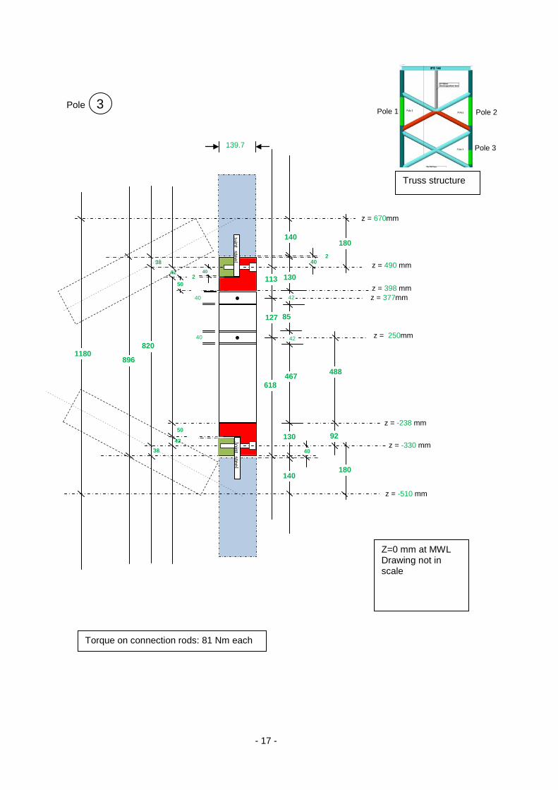
Attachment I - Dimensions of the local force transducer sections (Pole 1,2,3)
Page 61
- 15 -
Pole
320
150
42
42
42
42
150
87
151
40
1
40
40
40
139.7
820
896
38
38 42 50
42 337
130
108
45
108
140
z = 770 mm
z = 1063mm
z = 1150mm
z = 1300mm
z = 1450mm
Z=0 mm at MWL Drawing not in scale
180
180
z = 950mm
113
1180
z = 1770mm
z = 1950mm
140
40
40
Joint steel
2
2 40
Joint steel
50
Truss structure
Pole 1 Pole 2
Pole 3
Torque on connection rods: 81 Nm each
Page 62
- 16 -
Pole
320
150
42
42
42
42
150
87
151
40
2
40
40
40
139.7
820
896
38
38 42 50
42 337
130
108
45
108
140
z = 770 mm
z = 1063mm
z = 1150mm
z = 1300mm
z = 1450mm
Z=0 mm at MWL Drawing not in scale
180
180
z = 950mm
113
1180
z = 1770mm
z = 1950mm
140
40
40
Joint steel
Joint steel
2
2 40
50 207
Truss structure
Pole 1 Pole 2
Pole 3
Torque on connection rods: 81 Nm each
Page 63
- 17 -
Pole
113
127
618
3
40
139.7
820
896
38
38 42 50
42 130
130
85
467
140
z = -510 mm
z = 250mm
z = 377mm
Z=0 mm at MWL Drawing not in scale
180
180
92
1180
z = 490 mm
z = 670mm
140
40
40
Joint steel
Joint steel
2
2 40
50 z = 398 mm 40
42
42
z = -330 mm
z = -238 mm
488
Torque on connection rods: 81 Nm each
Truss structure
Pole 1 Pole 2
Pole 3