Preliminary Design of a Demonstration Heat Pump/AC Unit

Galway – Mayo Institute of Technology GMIT

2010/2011

Preliminary Design of

a Demonstration Heat

Pump/AC Unit MECHANICAL ENGINEERING: MAJOR PROJECT

FINAL REPORT

Author: Santiago Miguel de Ena Wolf (G00280356)

GMIT Supervisor: Oliver Mulryan

EUITIZ Supervisor: Francisco Javier Martínez

MAJOR PROJECT: Preliminary Design Of A Demonstration Heat Pump/AC Unit

FINAL TERM REPORT

2

INDEX

1. INTRODUCTION Page 5

2. BACKGROUND Page 7

2.1 Basic Theory of Heat Pumps Page 7

2.2 The Carnot Heat Pump (Reversible Heat Pump) Page 8

2.3 The Idealized Vapour Compression Cycle Page 10

2.4 The Actual Vapour Compression Cycle Page 11

2.5 Cooling and Heating with Heat Pump Systems Page 12

2.6 Heat Pump Components Page 13

2.7 Refrigerants Page 16

3. PROCEDURE Page 17

3.1 Observation and Elements in AC/Heat Pump System Page 17

3.2 Acquiring of the Compressor and Low & High Pressures Page 19

3.3 Calculation of Ideal-Vapour Compression Cycle Page 20

3.4 Calculation of Carnot COP and Actual COPs Page 22

3.5 Defining the Motor to drive the Compressor Page 23

3.6 Refrigerant Mass Flow Page 25

3.7 Isentropic Efficiency of the Compressor Page 25

3.8 Final Point of the diagram (Point 2) and Compression Ratio Page 26

3.9 Condenser and Evaporator Air Mass Flow Rate Page 28

3.10 Condenser and Evaporator Heat Transfer Calculations Page 29

3.11 Tubing Calculations Page 35

3.12 Heat Transfer coefficients for air in Condenser and Evaporator Page 36

4. CONCLUSION Page 40

5. BIBLIOGRAPHY Page 41

6. APPENDIX Page 42


FINAL TERM REPORT

3

TABLE OF FIGURES

2. BACKGROUND

2.1 Energy Fluxes in a Heat Pump Page 7

2.2 Thermodynamic Carnot Refrigeration Cycle Page 8

2.3 Processes in the Idealized Vapour Compression Cycle Page 10

2.4 Ideal vs Actual Vapour Compression Cycle (P-h and T-s) Page 11

2.5 Heat Pump mode – AC mode Page 12

2.6 Heat Pump Components (Schematic) Page 13

2.7 Piston Compressor Positions Page 13

2.8 Scroll Compressor Positions Page 14

2.9 Reversing Valve Positions and Operating Method Page 14

2.10 Sight Glass/Moisture Indicator Page 15

2.11 Bi-Flow Filter/Dryer flows Schema Page 15

2.12 Accumulator/Receiver Schema and Views Page 15

2.13 High and Low Real Pressostat Page 16

3. PROCEDURE

3.1 AC Unit Front View Page 17

3.2 AC Unit Side View with elements tagged Page 18

3.3 AC Unit Opposite Side View with elements tagged Page 18

3.4 Heat Pump/AC System with extra elements tagged Page 19

3.5 Pressure-Enthalpy Actual Refrigeration Diagram for R-134a Page 20

3.6 Compressor DELPHI 5106 SD7H15 Performance Page 23

3.7 P-v Compressor Diagram Page 25

3.8 Cross-Flow Heat Exchanger (Refrigerant Fluid and Gas Flows) Page 29

3.9 Correction Factor (F) Plots for single pass counter-flow heat exchanger,

both fluids unmixed Page 30

3.10 Condenser Inlet and Outlet Temperatures Sketch Page 31

3.11 Evaporator Inlet and Outlet Temperatures Sketch Page 33

3.12 Copper Tubing Cross-Section Page 36

3.13 Condenser Modelled as Air Flow over Staggered Pipes Page 37

3.14 Evaporator Modelled as Air Flow over Staggered Pipes Page 38


FINAL TERM REPORT

4

TABLE OF APPENDIXES

6. APPENDIX

6.1 Refrigerant R134a Saturated Properties (liquid-vapour): Temperature chart Page 42

6.2 Refrigerant R134a Saturated Properties (liquid-vapour): Temperature chart Page 43

6.3 Refrigerant R134a Superheated Vapour Properties Page 44


FINAL TERM REPORT

5

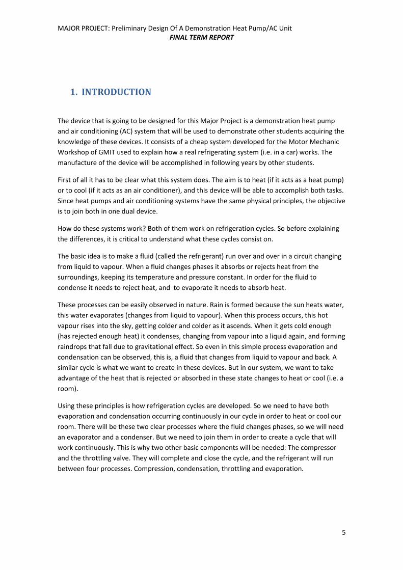
1. INTRODUCTION

The device that is going to be designed for this Major Project is a demonstration heat pump

and air conditioning (AC) system that will be used to demonstrate other students acquiring the

knowledge of these devices. It consists of a cheap system developed for the Motor Mechanic

Workshop of GMIT used to explain how a real refrigerating system (i.e. in a car) works. The

manufacture of the device will be accomplished in following years by other students.

First of all it has to be clear what this system does. The aim is to heat (if it acts as a heat pump)

or to cool (if it acts as an air conditioner), and this device will be able to accomplish both tasks.

Since heat pumps and air conditioning systems have the same physical principles, the objective

is to join both in one dual device.

How do these systems work? Both of them work on refrigeration cycles. So before explaining

the differences, it is critical to understand what these cycles consist on.

The basic idea is to make a fluid (called the refrigerant) run over and over in a circuit changing

from liquid to vapour. When a fluid changes phases it absorbs or rejects heat from the

surroundings, keeping its temperature and pressure constant. In order for the fluid to

condense it needs to reject heat, and to evaporate it needs to absorb heat.

These processes can be easily observed in nature. Rain is formed because the sun heats water,

this water evaporates (changes from liquid to vapour). When this process occurs, this hot

vapour rises into the sky, getting colder and colder as it ascends. When it gets cold enough

(has rejected enough heat) it condenses, changing from vapour into a liquid again, and forming

raindrops that fall due to gravitational effect. So even in this simple process evaporation and

condensation can be observed, this is, a fluid that changes from liquid to vapour and back. A

similar cycle is what we want to create in these devices. But in our system, we want to take

advantage of the heat that is rejected or absorbed in these state changes to heat or cool (i.e. a

room).

Using these principles is how refrigeration cycles are developed. So we need to have both

evaporation and condensation occurring continuously in our cycle in order to heat or cool our

room. There will be these two clear processes where the fluid changes phases, so we will need

an evaporator and a condenser. But we need to join them in order to create a cycle that will

work continuously. This is why two other basic components will be needed: The compressor

and the throttling valve. They will complete and close the cycle, and the refrigerant will run

between four processes. Compression, condensation, throttling and evaporation.


FINAL TERM REPORT

6

These four processes will be explained briefly, and afterwards will be looked at more deeply.

1.) The refrigerant will be compressed, to rise its temperature and pressure

2.) Next it condensates, so it rejects heat to the surroundings without changing its high

pressure and temperature. This rejected heat by the refrigerant will be the one that

we will use to heat the room (it’s the heat we need to work as a HEAT PUMP)

3.) A throttling process is then established, where the refrigerant lowers its pressure

without losing any internal energy. This will join condensation and evaporation.

4.) And finally the fluid will evaporate, so it absorbs heat from the surroundings

without changing its new low pressure and temperature. This absorbed heat by the

refrigerant will be the one that we will use to cool the room (it’s the heat we need to

work as an AIR CONDITIONER). After this process, the refrigerant goes again into the

compressor to continue with the cycle once again.

Even though our objective is to take advantage from the heat in condenser and evaporator,

the compressor is the main element of the cycle, the “heart”. It imposes high and low

pressures, which are the most important parameters to define these cycles. The aim of this

element is to elevate the pressure of the refrigerant, which is in gas state. Here is where the

energy is added in form of mechanical work for this cycle to run, following Thermodynamics

Laws.

Other auxiliary elements will be used, such as filters and dryers, and there will be a more

extended explanation of the theory and elements used in the Theory Part in the report.

In conclusion, an air conditioner’s aim is to extract heat from the surroundings (cooling them),

and heat pump’s is to reject heat to these surroundings (heating them). Having both heat

pump and AC in only one device will make understanding easier and this project was needed

for the Lecturers area.

This project will also analyze the heat transfer area of the device. It’s easy to recognize where

heat is exchanged, this is, what components actuate in this way: evaporator and condenser. So

in these components it’s important to know how efficiently this heat is exchanged, what are

the heat transfer coefficients that drive this heat exchange, how big should evaporator and

condenser be, etc.


FINAL TERM REPORT

7

2. BACKGROUND

2.1 Basic Theory of Heat Pumps

The relevant Theory applied in this project will be mainly based on Thermodynamics. As briefly

explained in the Introduction, a heat pump is a device that works acquiring heat from a source

and releasing heat in a different place, using an external for this process. Basically, pumping

heat from a cold source to a hot one is what heat pumps do. This work input is absolutely

necessary because as we can experiment, heat naturally flows from a hot object to a cold one.

But to make heat go the other way around (“counter nature”) an external work source is

needed. This is because heat pumps work according to a refrigeration cycle, as explained in the

Introduction, and every cycle has to be in accordance with Modernised Clausius Statement on

the Second Law of Thermodynamics:

“It is impossible to construct a Heat Pump/Refrigerator which operates on a cycle,

which requires no work input from the surroundings to transfer heat from a low

temperature reservoir to the high temperature reservoir”.

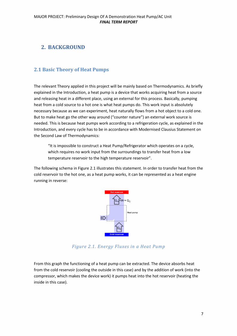
The following schema in Figure 2.1 illustrates this statement. In order to transfer heat from the

cold reservoir to the hot one, as a heat pump works, it can be represented as a heat engine

running in reverse:

Figure 2.1. Energy Fluxes in a Heat Pump

From this graph the functioning of a heat pump can be extracted. The device absorbs heat

from the cold reservoir (cooling the outside in this case) and by the addition of work (into the

compressor, which makes the device work) it pumps heat into the hot reservoir (heating the

inside in this case).


FINAL TERM REPORT

8

2.2 The Carnot Heat Pump (Reversible Heat Pump)

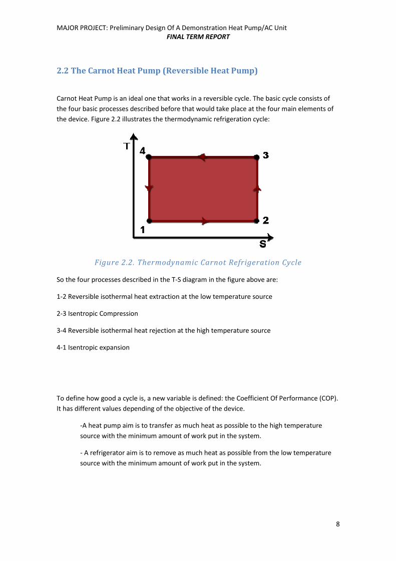
Carnot Heat Pump is an ideal one that works in a reversible cycle. The basic cycle consists of

the four basic processes described before that would take place at the four main elements of

the device. Figure 2.2 illustrates the thermodynamic refrigeration cycle:

Figure 2.2. Thermodynamic Carnot Refrigeration Cycle

So the four processes described in the T-S diagram in the figure above are:

1-2 Reversible isothermal heat extraction at the low temperature source

2-3 Isentropic Compression

3-4 Reversible isothermal heat rejection at the high temperature source

4-1 Isentropic expansion

To define how good a cycle is, a new variable is defined: the Coefficient Of Performance (COP).

It has different values depending of the objective of the device.

-A heat pump aim is to transfer as much heat as possible to the high temperature

source with the minimum amount of work put in the system.

- A refrigerator aim is to remove as much heat as possible from the low temperature

source with the minimum amount of work put in the system.


FINAL TERM REPORT

9

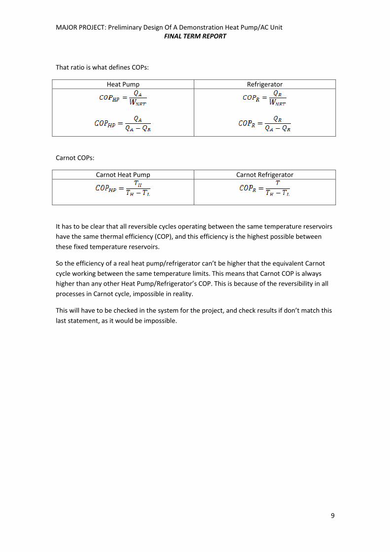
That ratio is what defines COPs:

Heat Pump Refrigerator

Carnot COPs:

Carnot Heat Pump Carnot Refrigerator

It has to be clear that all reversible cycles operating between the same temperature reservoirs

have the same thermal efficiency (COP), and this efficiency is the highest possible between

these fixed temperature reservoirs.

So the efficiency of a real heat pump/refrigerator can’t be higher that the equivalent Carnot

cycle working between the same temperature limits. This means that Carnot COP is always

higher than any other Heat Pump/Refrigerator’s COP. This is because of the reversibility in all

processes in Carnot cycle, impossible in reality.

This will have to be checked in the system for the project, and check results if don’t match this

last statement, as it would be impossible.


FINAL TERM REPORT

10

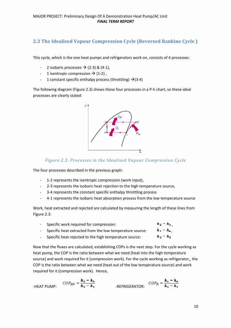
2.3 The Idealised Vapour Compression Cycle (Reversed Rankine Cycle )

This cycle, which is the one heat pumps and refrigerators work on, consists of 4 processes:

- 2 isobaric processes � (2-3) & (4-1),

- 1 isentropic compression � (1-2) ,

- 1 constant specific enthalpy process (throttling) �(3-4)

The following diagram (Figure 2.3) shows these four processes in a P-h chart, so these ideal

processes are clearly stated:

Figure 2.3. Processes in the Idealised Vapour Compression Cycle

The four processes described in the previous graph:

- 1-2 represents the isentropic compression (work input),

- 2-3 represents the isobaric heat rejection to the high temperature source,

- 3-4 represents the constant specific enthalpy throttling process

- 4-1 represents the isobaric heat absorption process from the low temperature source

Work, heat extracted and rejected are calculated by measuring the length of these lines from

Figure 2.3:

- Specific work required for compression: ,

- Specific heat extracted from the low temperature source: ,

- Specific heat rejected to the high temperature source:

Now that the fluxes are calculated, establishing COPs is the next step. For the cycle working as

heat pump, the COP is the ratio between what we need (heat into the high temperature

source) and work required for it (compression work). For the cycle working as refrigerator,, the

COP is the ratio between what we need (heat out of the low temperature source) and work

required for it (compression work). Hence,

-HEAT PUMP: -REFRIGERATOR:


FINAL TERM REPORT

11

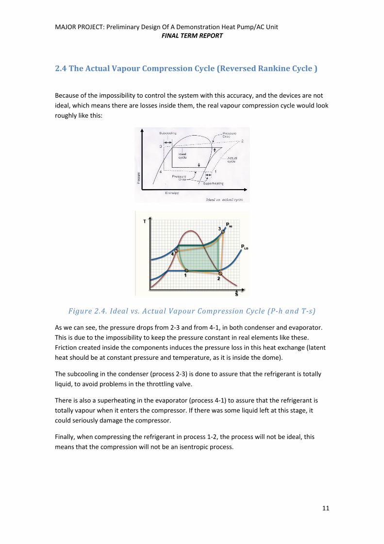
2.4 The Actual Vapour Compression Cycle (Reversed Rankine Cycle )

Because of the impossibility to control the system with this accuracy, and the devices are not

ideal, which means there are losses inside them, the real vapour compression cycle would look

roughly like this:

Figure 2.4. Ideal vs. Actual Vapour Compression Cycle (P-h and T-s)

As we can see, the pressure drops from 2-3 and from 4-1, in both condenser and evaporator.

This is due to the impossibility to keep the pressure constant in real elements like these.

Friction created inside the components induces the pressure loss in this heat exchange (latent

heat should be at constant pressure and temperature, as it is inside the dome).

The subcooling in the condenser (process 2-3) is done to assure that the refrigerant is totally

liquid, to avoid problems in the throttling valve.

There is also a superheating in the evaporator (process 4-1) to assure that the refrigerant is

totally vapour when it enters the compressor. If there was some liquid left at this stage, it

could seriously damage the compressor.

Finally, when compressing the refrigerant in process 1-2, the process will not be ideal, this

means that the compression will not be an isentropic process.


FINAL TERM REPORT

12

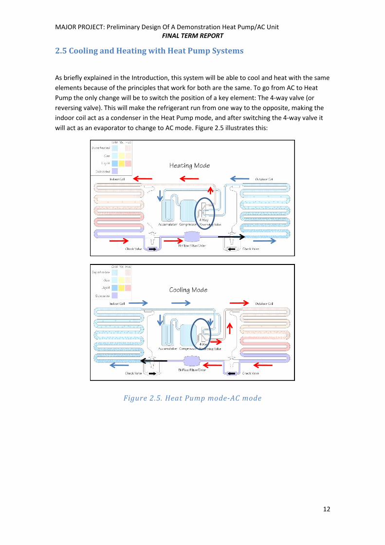
2.5 Cooling and Heating with Heat Pump Systems

As briefly explained in the Introduction, this system will be able to cool and heat with the same

elements because of the principles that work for both are the same. To go from AC to Heat

Pump the only change will be to switch the position of a key element: The 4-way valve (or

reversing valve). This will make the refrigerant run from one way to the opposite, making the

indoor coil act as a condenser in the Heat Pump mode, and after switching the 4-way valve it

will act as an evaporator to change to AC mode. Figure 2.5 illustrates this:

Figure 2.5. Heat Pump mode-AC mode


FINAL TERM REPORT

13

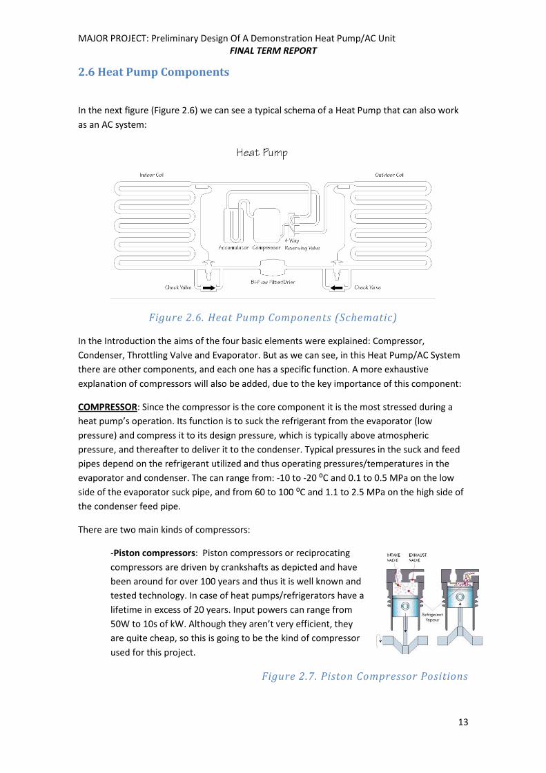
2.6 Heat Pump Components

In the next figure (Figure 2.6) we can see a typical schema of a Heat Pump that can also work

as an AC system:

Figure 2.6. Heat Pump Components (Schematic)

In the Introduction the aims of the four basic elements were explained: Compressor,

Condenser, Throttling Valve and Evaporator. But as we can see, in this Heat Pump/AC System

there are other components, and each one has a specific function. A more exhaustive

explanation of compressors will also be added, due to the key importance of this component:

COMPRESSOR: Since the compressor is the core component it is the most stressed during a

heat pump’s operation. Its function is to suck the refrigerant from the evaporator (low

pressure) and compress it to its design pressure, which is typically above atmospheric

pressure, and thereafter to deliver it to the condenser. Typical pressures in the suck and feed

pipes depend on the refrigerant utilized and thus operating pressures/temperatures in the

evaporator and condenser. The can range from: -10 to -20 ⁰C and 0.1 to 0.5 MPa on the low

side of the evaporator suck pipe, and from 60 to 100 ⁰C and 1.1 to 2.5 MPa on the high side of

the condenser feed pipe.

There are two main kinds of compressors:

-Piston compressors: Piston compressors or reciprocating

compressors are driven by crankshafts as depicted and have

been around for over 100 years and thus it is well known and

tested technology. In case of heat pumps/refrigerators have a

lifetime in excess of 20 years. Input powers can range from

50W to 10s of kW. Although they aren’t very efficient, they

are quite cheap, so this is going to be the kind of compressor

used for this project.

Figure 2.7. Piston Compressor Positions


FINAL TERM REPORT

14

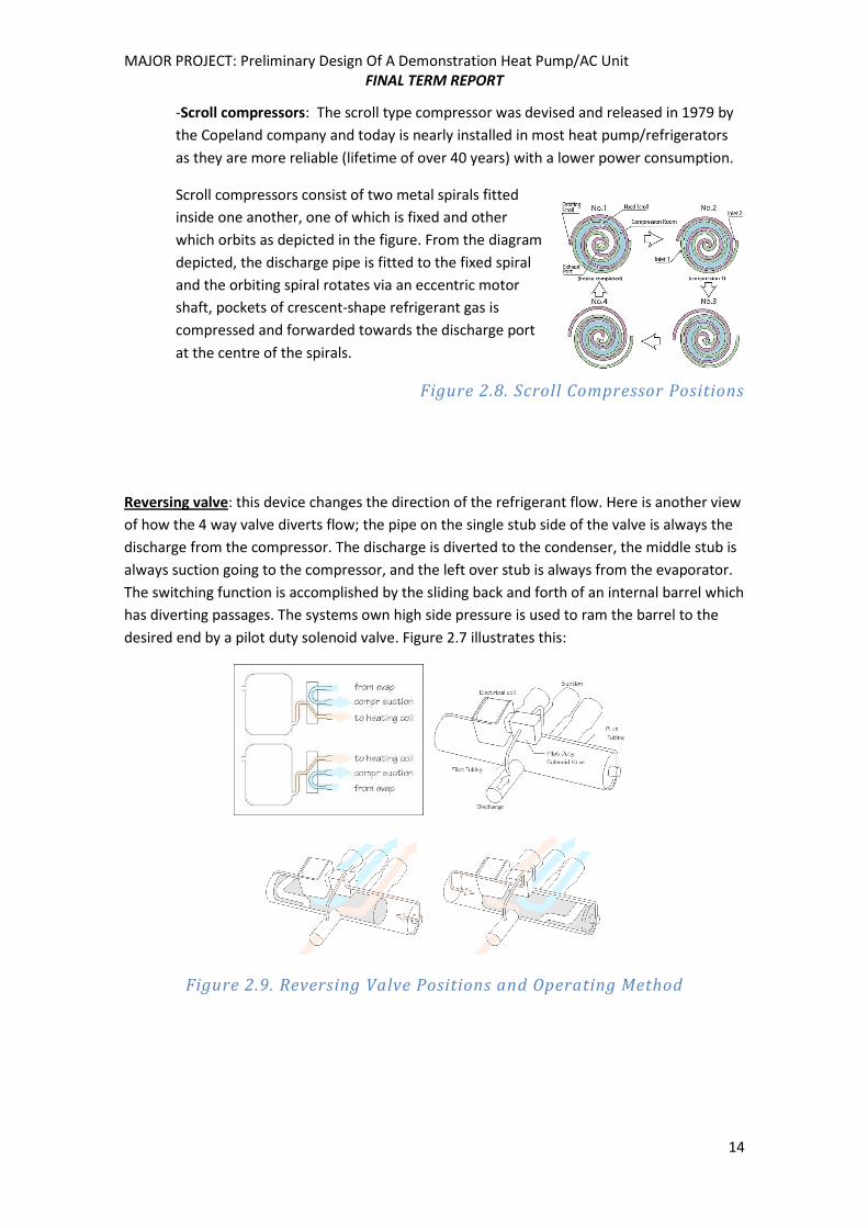
-Scroll compressors: The scroll type compressor was devised and released in 1979 by

the Copeland company and today is nearly installed in most heat pump/refrigerators

as they are more reliable (lifetime of over 40 years) with a lower power consumption.

Scroll compressors consist of two metal spirals fitted

inside one another, one of which is fixed and other

which orbits as depicted in the figure. From the diagram

depicted, the discharge pipe is fitted to the fixed spiral

and the orbiting spiral rotates via an eccentric motor

shaft, pockets of crescent-shape refrigerant gas is

compressed and forwarded towards the discharge port

at the centre of the spirals.

Figure 2.8. Scroll Compressor Positions

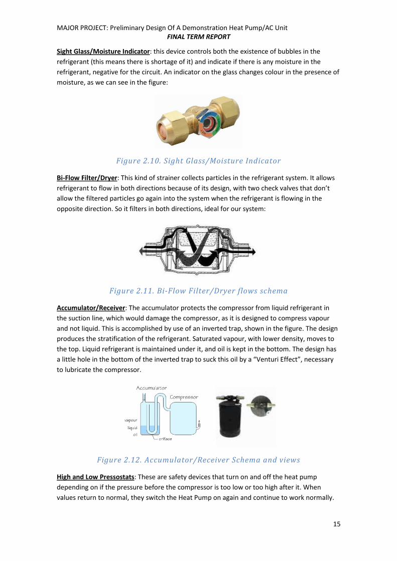
Reversing valve: this device changes the direction of the refrigerant flow. Here is another view

of how the 4 way valve diverts flow; the pipe on the single stub side of the valve is always the

discharge from the compressor. The discharge is diverted to the condenser, the middle stub is

always suction going to the compressor, and the left over stub is always from the evaporator.

The switching function is accomplished by the sliding back and forth of an internal barrel which

has diverting passages. The systems own high side pressure is used to ram the barrel to the

desired end by a pilot duty solenoid valve. Figure 2.7 illustrates this:

Figure 2.9. Reversing Valve Positions and Operating Method


FINAL TERM REPORT

15

Sight Glass/Moisture Indicator: this device controls both the existence of bubbles in the

refrigerant (this means there is shortage of it) and indicate if there is any moisture in the

refrigerant, negative for the circuit. An indicator on the glass changes colour in the presence of

moisture, as we can see in the figure:

Figure 2.10. Sight Glass/Moisture Indicator

Bi-Flow Filter/Dryer: This kind of strainer collects particles in the refrigerant system. It allows

refrigerant to flow in both directions because of its design, with two check valves that don’t

allow the filtered particles go again into the system when the refrigerant is flowing in the

opposite direction. So it filters in both directions, ideal for our system:

Figure 2.11. Bi-Flow Filter/Dryer flows schema

Accumulator/Receiver: The accumulator protects the compressor from liquid refrigerant in

the suction line, which would damage the compressor, as it is designed to compress vapour

and not liquid. This is accomplished by use of an inverted trap, shown in the figure. The design

produces the stratification of the refrigerant. Saturated vapour, with lower density, moves to

the top. Liquid refrigerant is maintained under it, and oil is kept in the bottom. The design has

a little hole in the bottom of the inverted trap to suck this oil by a “Venturi Effect”, necessary

to lubricate the compressor.

Figure 2.12. Accumulator/Receiver Schema and views

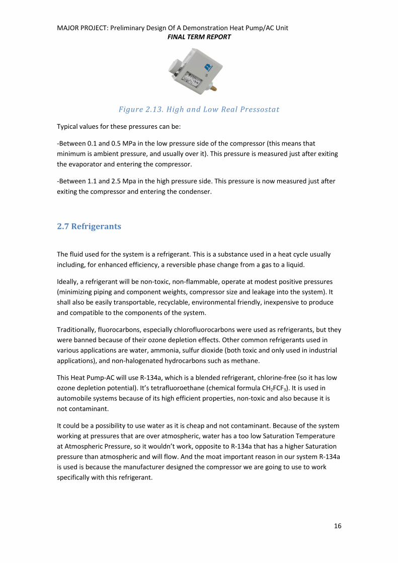
High and Low Pressostats: These are safety devices that turn on and off the heat pump

depending on if the pressure before the compressor is too low or too high after it. When

values return to normal, they switch the Heat Pump on again and continue to work normally.


FINAL TERM REPORT

16

Figure 2.13. High and Low Real Pressostat

Typical values for these pressures can be:

-Between 0.1 and 0.5 MPa in the low pressure side of the compressor (this means that

minimum is ambient pressure, and usually over it). This pressure is measured just after exiting

the evaporator and entering the compressor.

-Between 1.1 and 2.5 Mpa in the high pressure side. This pressure is now measured just after

exiting the compressor and entering the condenser.

2.7 Refrigerants

The fluid used for the system is a refrigerant. This is a substance used in a heat cycle usually

including, for enhanced efficiency, a reversible phase change from a gas to a liquid.

Ideally, a refrigerant will be non-toxic, non-flammable, operate at modest positive pressures

(minimizing piping and component weights, compressor size and leakage into the system). It

shall also be easily transportable, recyclable, environmental friendly, inexpensive to produce

and compatible to the components of the system.

Traditionally, fluorocarbons, especially chlorofluorocarbons were used as refrigerants, but they

were banned because of their ozone depletion effects. Other common refrigerants used in

various applications are water, ammonia, sulfur dioxide (both toxic and only used in industrial

applications), and non-halogenated hydrocarbons such as methane.

This Heat Pump-AC will use R-134a, which is a blended refrigerant, chlorine-free (so it has low

ozone depletion potential). It’s tetrafluoroethane (chemical formula CH2FCF3). It is used in

automobile systems because of its high efficient properties, non-toxic and also because it is

not contaminant.

It could be a possibility to use water as it is cheap and not contaminant. Because of the system

working at pressures that are over atmospheric, water has a too low Saturation Temperature

at Atmospheric Pressure, so it wouldn’t work, opposite to R-134a that has a higher Saturation

pressure than atmospheric and will flow. And the moat important reason in our system R-134a

is used is because the manufacturer designed the compressor we are going to use to work

specifically with this refrigerant.


FINAL TERM REPORT

17

3. PROCEDURE

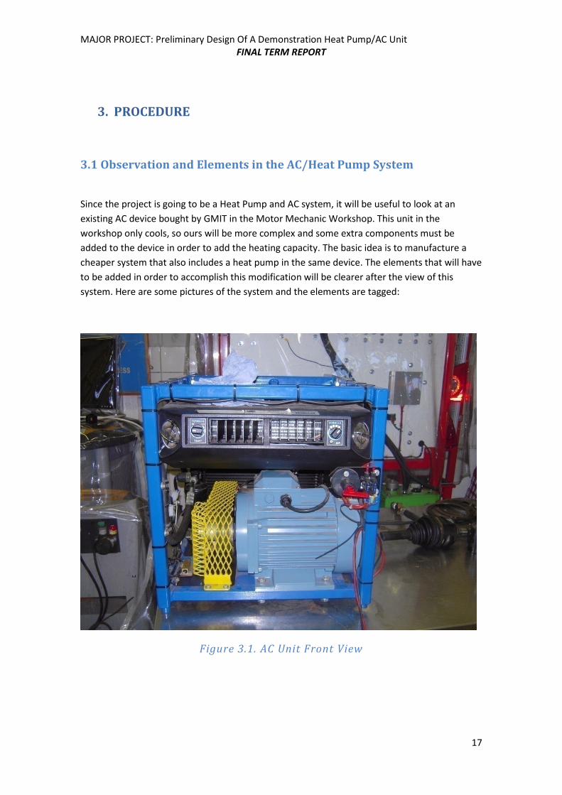
3.1 Observation and Elements in the AC/Heat Pump System

Since the project is going to be a Heat Pump and AC system, it will be useful to look at an

existing AC device bought by GMIT in the Motor Mechanic Workshop. This unit in the

workshop only cools, so ours will be more complex and some extra components must be

added to the device in order to add the heating capacity. The basic idea is to manufacture a

cheaper system that also includes a heat pump in the same device. The elements that will have

to be added in order to accomplish this modification will be clearer after the view of this

system. Here are some pictures of the system and the elements are tagged:

Figure 3.1. AC Unit Front View


FINAL TERM REPORT

18

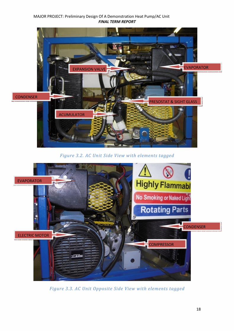
Figure 3.2. AC Unit Side View with elements tagged

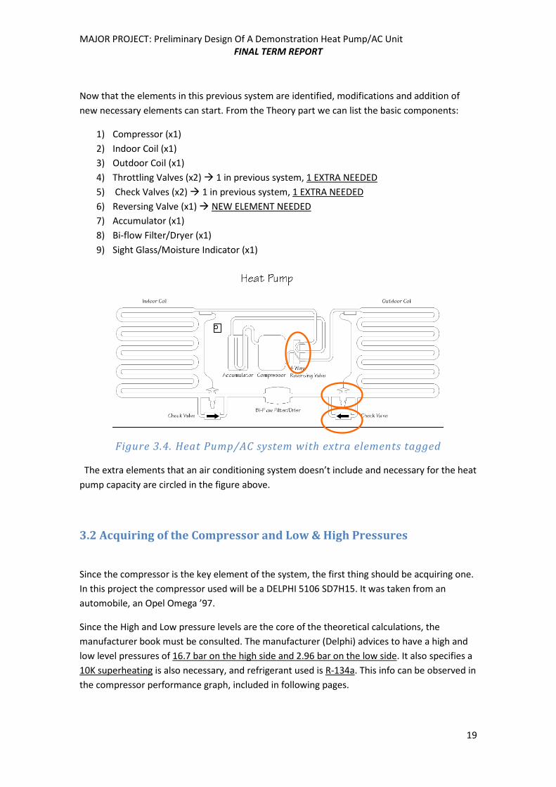
Figure 3.3. AC Unit Opposite Side View with elements tagged

CONDENSER

ACUMULATOR

EVAPORATOR

PRESOSTAT & SIGHT GLASS

EXPANSION VALVE

EVAPORATOR

ELECTRIC MOTOR

CONDENSER

COMPRESSOR


FINAL TERM REPORT

19

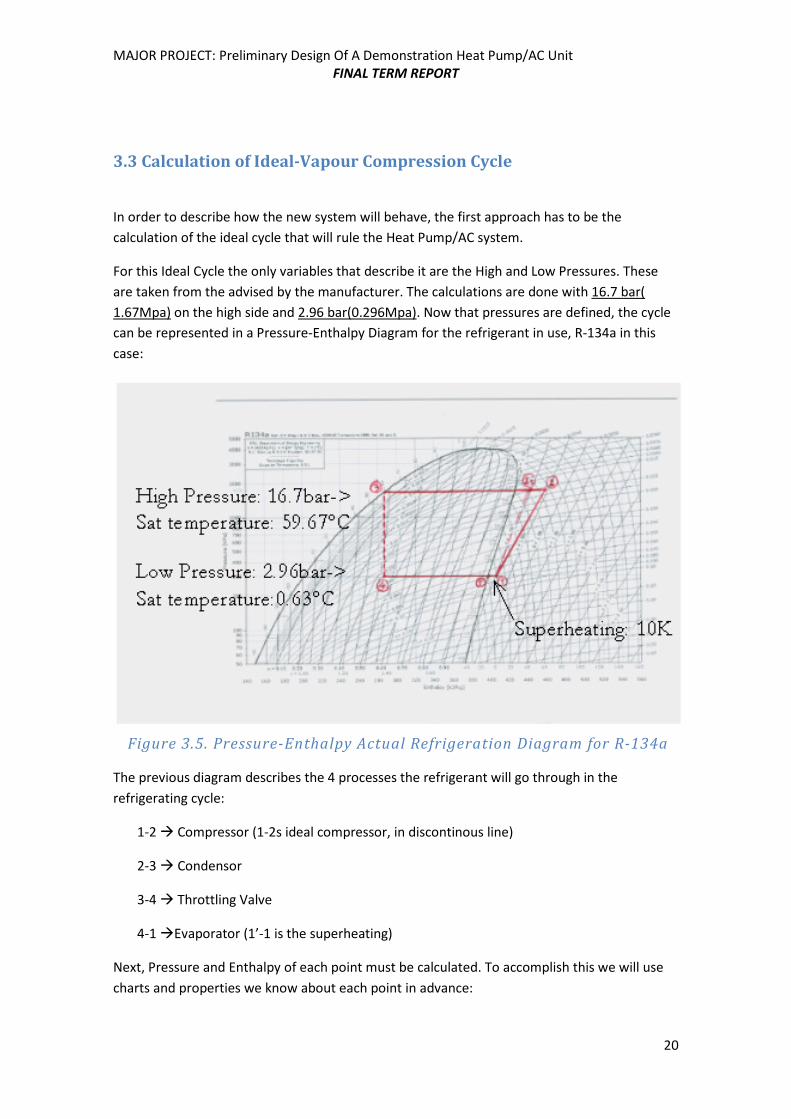
Now that the elements in this previous system are identified, modifications and addition of

new necessary elements can start. From the Theory part we can list the basic components:

1) Compressor (x1)

2) Indoor Coil (x1)

3) Outdoor Coil (x1)

4) Throttling Valves (x2) � 1 in previous system, 1 EXTRA NEEDED

5) Check Valves (x2) � 1 in previous system, 1 EXTRA NEEDED

6) Reversing Valve (x1) � NEW ELEMENT NEEDED

7) Accumulator (x1)

8) Bi-flow Filter/Dryer (x1)

9) Sight Glass/Moisture Indicator (x1)

Figure 3.4. Heat Pump/AC system with extra elements tagged

The extra elements that an air conditioning system doesn’t include and necessary for the heat

pump capacity are circled in the figure above.

3.2 Acquiring of the Compressor and Low & High Pressures

Since the compressor is the key element of the system, the first thing should be acquiring one.

In this project the compressor used will be a DELPHI 5106 SD7H15. It was taken from an

automobile, an Opel Omega ’97.

Since the High and Low pressure levels are the core of the theoretical calculations, the

manufacturer book must be consulted. The manufacturer (Delphi) advices to have a high and

low level pressures of 16.7 bar on the high side and 2.96 bar on the low side. It also specifies a

10K superheating is also necessary, and refrigerant used is R-134a. This info can be observed in

the compressor performance graph, included in following pages.


FINAL TERM REPORT

20

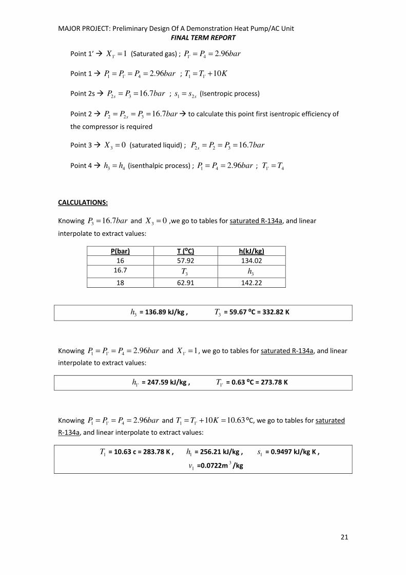
3.3 Calculation of Ideal-Vapour Compression Cycle

In order to describe how the new system will behave, the first approach has to be the

calculation of the ideal cycle that will rule the Heat Pump/AC system.

For this Ideal Cycle the only variables that describe it are the High and Low Pressures. These

are taken from the advised by the manufacturer. The calculations are done with 16.7 bar(

1.67Mpa) on the high side and 2.96 bar(0.296Mpa). Now that pressures are defined, the cycle

can be represented in a Pressure-Enthalpy Diagram for the refrigerant in use, R-134a in this

case:

Figure 3.5. Pressure-Enthalpy Actual Refrigeration Diagram for R-134a

The previous diagram describes the 4 processes the refrigerant will go through in the

refrigerating cycle:

1-2 � Compressor (1-2s ideal compressor, in discontinous line)

2-3 � Condensor

3-4 � Throttling Valve

4-1 �Evaporator (1’-1 is the superheating)

Next, Pressure and Enthalpy of each point must be calculated. To accomplish this we will use

charts and properties we know about each point in advance:


FINAL TERM REPORT

21

Point 1’ � 1'1 =X (Saturated gas) ; barPP 96.24'1 ==

Point 1 � barPPP 96.24'11 === ; KTT 10'11 +=

Point 2s � barPP s 7.1632 == ; sss 21 = (Isentropic process)

Point 2 � barPPP s 7.16322 === � to calculate this point first isentropic efficiency of

the compressor is required

Point 3 � 03 =X (saturated liquid) ; barPPP s 7.16322 ===

Point 4 � 43 hh = (isenthalpic process) ; barPP 96.241 == ; 4'1 TT =

CALCULATIONS:

Knowing barP 7.163 = and 03 =X ,we go to tables for saturated R-134a, and linear

interpolate to extract values:

P(bar) T (⁰C) h(kJ/kg)

16 57.92 134.02

16.7 3T 3h

18 62.91 142.22

3h = 136.89 kJ/kg , 3T = 59.67 ⁰C = 332.82 K

Knowing barPPP 96.24'11 === and 1'1 =X , we go to tables for saturated R-134a, and linear

interpolate to extract values:

'1h = 247.59 kJ/kg , '1T = 0.63 ⁰C = 273.78 K

Knowing barPPP 96.24'11 === and 63.1010'11 =+= KTT ⁰C, we go to tables for saturated

R-134a, and linear interpolate to extract values:

1T = 10.63 c = 283.78 K , 1h = 256.21 kJ/kg , 1s = 0.9497 kJ/kg K ,

1v =0.0722m3

/kg


FINAL TERM REPORT

22

Knowing kgKkJss s /9497.021 == and barPPP s 7.16322 === , we go to tables for

saturated R-134a, and linear interpolate to extract values:

sh2 = 292.33 kJ/kg

Knowing barPP 96.24'1 == , 4'1 TT = and 43 hh = ,we calculate Point 4:

4h = 136.89 kJ/kg , 4T = 0.63 ⁰C = 273.78 K

Now all 5 points are defined, the Diagram can be completed and COPs can now be calculated

(expected efficiencies).

3.4 Calculation of Carnot COP and Actual COPs

Now all 4 points are defined, COPs will be calculated. COPs indicate the efficiency of

refrigeration devices, by indicating what factor multiplies the work put into the system to

obtain a certain quantity of heat (extracted or rejected, depending on if the device works as a

Heat Pump or a refrigerator).

For example, if and , for every 10kW inverted in the system as Work

in the compressor, the device will reject 3x10 = 30kW in Heat Pump Mode and 2x10 = 20kW in

Refrigerator Mode.

Moreover, as explained in the Theory, Actual COPs can never be greater than Carnot’s COPs, as

this last values are the highest possible between two fixed pressure values.

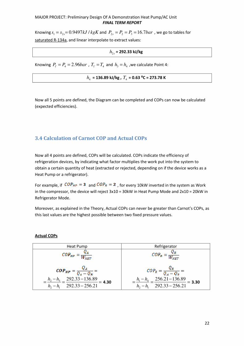
Actual COPs

Heat Pump Refrigerator

=−

−=

−

−=

21.25633.292

89.13633.292

12

32

hh

hh4.30

=−

−=

−

−=

21.25633.292

89.13621.256

12

41

hh

hh3.30


FINAL TERM REPORT

23

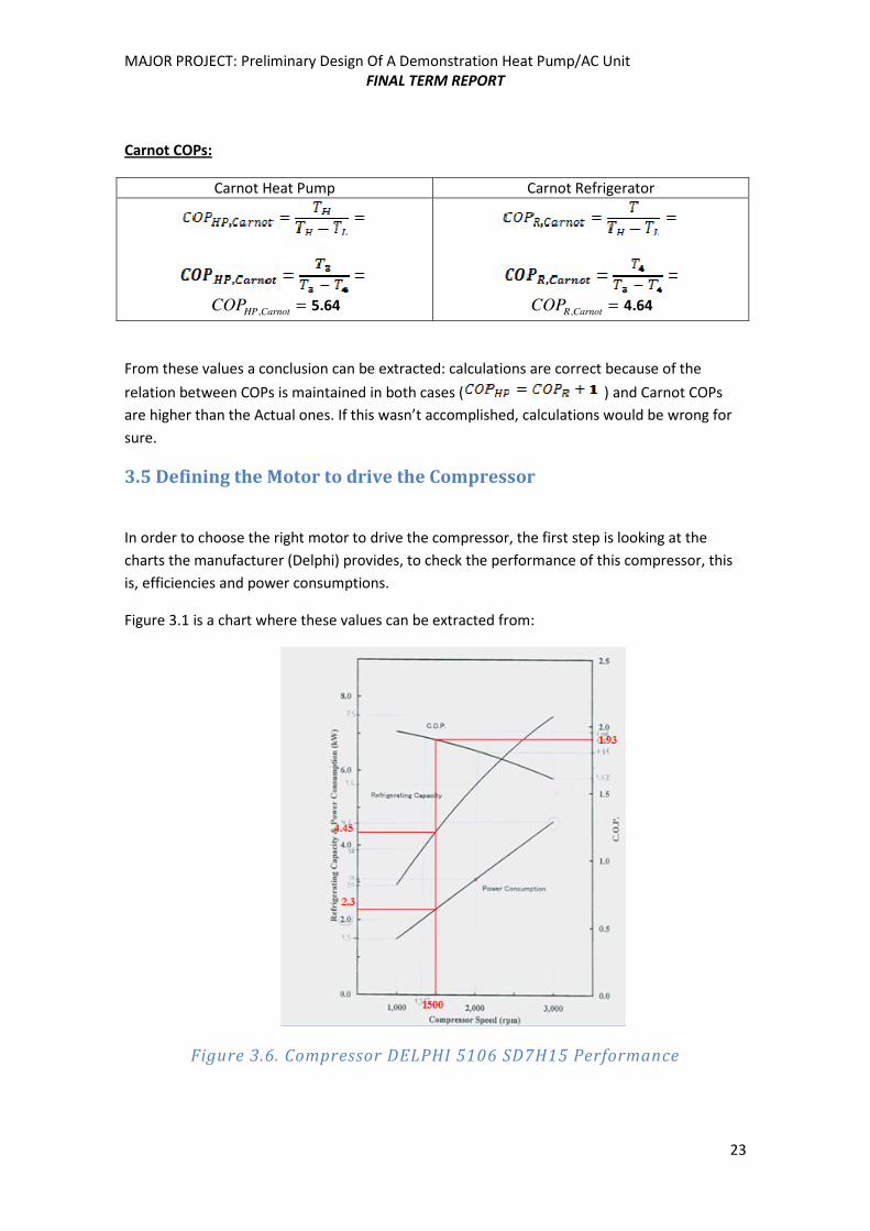
Carnot COPs:

Carnot Heat Pump Carnot Refrigerator

=CarnotHPCOP , 5.64

=CarnotRCOP , 4.64

From these values a conclusion can be extracted: calculations are correct because of the

relation between COPs is maintained in both cases ( ) and Carnot COPs

are higher than the Actual ones. If this wasn’t accomplished, calculations would be wrong for

sure.

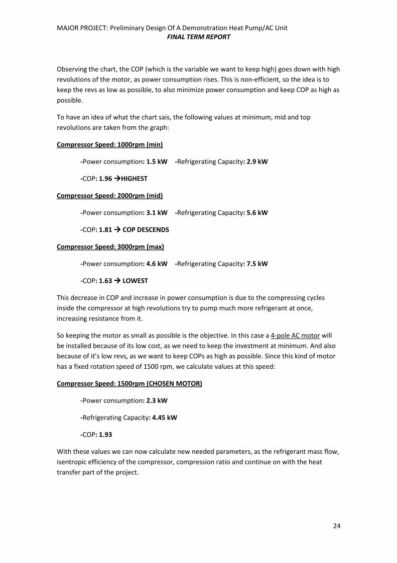
3.5 Defining the Motor to drive the Compressor

In order to choose the right motor to drive the compressor, the first step is looking at the

charts the manufacturer (Delphi) provides, to check the performance of this compressor, this

is, efficiencies and power consumptions.

Figure 3.1 is a chart where these values can be extracted from:

Figure 3.6. Compressor DELPHI 5106 SD7H15 Performance


FINAL TERM REPORT

24

Observing the chart, the COP (which is the variable we want to keep high) goes down with high

revolutions of the motor, as power consumption rises. This is non-efficient, so the idea is to

keep the revs as low as possible, to also minimize power consumption and keep COP as high as

possible.

To have an idea of what the chart sais, the following values at minimum, mid and top

revolutions are taken from the graph:

Compressor Speed: 1000rpm (min)

-Power consumption: 1.5 kW -Refrigerating Capacity: 2.9 kW

-COP: 1.96 ��HIGHEST

Compressor Speed: 2000rpm (mid)


-COP: 1.81 �� COP DESCENDS

Compressor Speed: 3000rpm (max)


-COP: 1.63 �� LOWEST

This decrease in COP and increase in power consumption is due to the compressing cycles

inside the compressor at high revolutions try to pump much more refrigerant at once,

increasing resistance from it.

So keeping the motor as small as possible is the objective. In this case a 4-pole AC motor will

be installed because of its low cost, as we need to keep the investment at minimum. And also

because of it’s low revs, as we want to keep COPs as high as possible. Since this kind of motor

has a fixed rotation speed of 1500 rpm, we calculate values at this speed:

Compressor Speed: 1500rpm (CHOSEN MOTOR)

-Power consumption: 2.3 kW

-Refrigerating Capacity: 4.45 kW

-COP: 1.93

With these values we can now calculate new needed parameters, as the refrigerant mass flow,

isentropic efficiency of the compressor, compression ratio and continue on with the heat

transfer part of the project.


FINAL TERM REPORT

25

3.6 Refrigerant Mass Flow

One very important parameter needed is the refrigerant mass flow. This is how much R134-a is

circulating through the device per unit time. This parameter is needed in order to calculate

powers, as all the energy units from the cycle previously calculated are per unit mass (kJ/kg).

Mass flow is expressed in kg/s , so it expresses how much mass is circulating per second. To

obtain this value, we are going to focus in the manufacturer data and our calculations.

Since we know how much heat is extracted from the cold reservoir in the evaporator from the

compressor performance (this is the Refrigeration Capacity of 4.45kW) and we also know the

enthalpies at the entrance and exit of the evaporator:

)( 14 hhmQevap −= &&

kgkJ

kW

hh

Qm

evap

/89.13621.256

45.4

14 −=

−=

&

&

m& = 0.0373 kg/s = 37.3 g/s

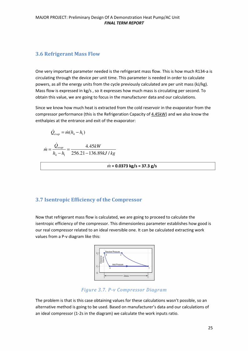
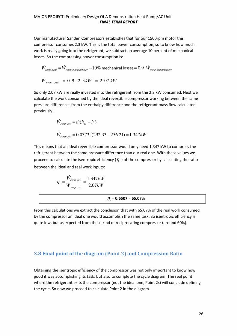
3.7 Isentropic Efficiency of the Compressor

Now that refrigerant mass flow is calculated, we are going to proceed to calculate the

isentropic efficiency of the compressor. This dimensionless parameter establishes how good is

our real compressor related to an ideal reversible one. It can be calculated extracting work

values from a P-v diagram like this:

Figure 3.7. P-v Compressor Diagram

The problem is that is this case obtaining values for these calculations wasn’t possible, so an

alternative method is going to be used. Based on manufacturer’s data and our calculations of

an ideal compressor (1-2s in the diagram) we calculate the work inputs ratio.


FINAL TERM REPORT

26

Our manufacturer Sanden Compressors establishes that for our 1500rpm motor the

compressor consumes 2.3 kW. This is the total power consumption, so to know how much

work is really going into the refrigerant, we subtract an average 10 percent of mechanical

losses. So the compressing power consumption is:

%10,, −= ermanufacturcomprealcomp WW && mechanical losses ermanufacturcompW ,9.0 &⋅=

kWkWW realcomp 07.23.29.0, =⋅=&

So only 2.07 kW are really invested into the refrigerant from the 2.3 kW consumed. Next we

calculate the work consumed by the ideal reversible compressor working between the same

pressure differences from the enthalpy difference and the refrigerant mass flow calculated

previously:

)( 12, hhmW srevcomp −= &&

kWW revcomp 347.1)21.25633.292(0373.0, =−⋅=&

This means that an ideal reversible compressor would only need 1.347 kW to compress the

refrigerant between the same pressure difference than our real one. With these values we

proceed to calculate the isentropic efficiency ( sη ) of the compressor by calculating the ratio

between the ideal and real work inputs:

kW

kW

W

W

realcomp

revcomp

s07.2

347.1

,

,==

&

&

η

sη = 0.6507 = 65.07%

From this calculations we extract the conclusion that with 65.07% of the real work consumed

by the compressor an ideal one would accomplish the same task. So isentropic efficiency is

quite low, but as expected from these kind of reciprocating compressor (around 60%).

3.8 Final point of the diagram (Point 2) and Compression Ratio

Obtaining the isentropic efficiency of the compressor was not only important to know how

good it was accomplishing its task, but also to complete the cycle diagram. The real point

where the refrigerant exits the compressor (not the ideal one, Point 2s) will conclude defining

the cycle. So now we proceed to calculate Point 2 in the diagram.


FINAL TERM REPORT

27

From the definition of isentropic efficiency, we can write:

realcomp

revcomp

sW

W

,

,=η

If we now substitute work inputs by enthalpy differences:

12

12

hh

hh ss

−

−=η

And extract 2h from this formula:

s

s hhhh

η12

12

−+=

6507.0

21.25633.29221.2562

−+=h = 311.72 kJ/kg

Now that we know enthalpy in Point 2( 2h = 311.72 kJ/kg) and pressure

( barPPP s 7.16322 === ), we go to tables for saturated R-134a, and linear interpolate to

extract values:

2T = 86.7⁰C , 2v = 0.0141 m3

/kg

With these last calculations, the whole cycle is defined, and Points 1, 1’, 2s, 2, 3 and 4 are

completely defined, so the diagram is complete.

Next step will be calculate the compression ratio, this is, how many times smaller is the same

mass of the high pressure compressed refrigerant exiting the compressor in comparison to the

low pressure refrigerant entering it. These compressors have a maximum compression ratio of

6. This means that for security reasons a constant value mass of refrigerant exiting the

compressor must be 6 times smaller that the one entering, as maximum. So now we proceed

to calculate this ratio (specific volume entering compressor over specific volume exiting):

Compression Ratio kgm

kgm

v

v

/0141.0

/0722.03

3

2

1 ==

2v = Compression Ratio = 5.12

Analyzing this result, we can conclude that our compressor is operating securely, as it doesn’t

exceed the compression ratio established.


FINAL TERM REPORT

28

3.9 Condenser and Evaporator Air Mass Flow Rate

Now that the thermodynamic diagram is completely defined, next step is to calculate how

much air do condenser and evaporator need in order to exchange the calculated heat. To

achieve this, an Energy Balance from 1st Law of Thermodynamics will be done on both

condenser and evaporator.

sistOUTOUT

ININ

UgzV

hmgzV

hmWQ ∆=++Σ−++Σ=− )2

()2

(22

&&&&

And from here we can assume:

-No kinetic energy variations (2

2V

= 0)

-No potential energy variations (gz = 0)

-Stationary system, there is no work/energy accumulated in the system ( sistU∆ = 0)

After using the assumptions, the balance is:

OUTOUT

ININ

hmhm && Σ=Σ

And substituting from what we know:

airairairaRaR Tcmhm ∆⋅⋅=∆ && )( 134134

With this last equation we calculate Air Mass Flow Rates ( airm& ) for both condenser and

evaporator

airair

aRaRair

Tc

hmm

∆⋅

∆=

)( 134134&

&

-specific heat of air ( airc )= 1.006 kJ/kgK

CONDENSER: The air temperatures entering and exiting the condenser are now needed. This

component is the one that rejects heat, heating the space required. We take the worst case

scenario of winter, where Met Eireann says that average temperature in Ireland’s winter is

about 8 ⁰C, and we take an even lower temperature to ensure or calculations. This ambient air

temperature is going to be taken as 5 ⁰C. The exiting temperature we want will be of 45 ⁰C to

heat the space fast. So with all data we substitute in the equation:

=−

−=

∆⋅

−=

)545(006.1

)89.13672.311(0373.0)( 32134,

airair

aRcondair

Tc

hhmm

&&


FINAL TERM REPORT

29

condairm ,& = 0.162 kg/s

EVAPORATOR: The air temperatures entering and exiting the evaporator are also needed. This

component is the one that absorbs heat, cooling the space desired. We take the worst case

scenario of summer, where Met Eireann says that average temperature in Ireland’s summer is

about 18-20 ⁰C, and we take an even higher temperature to ensure or calculations. This

ambient air temperature is going to be taken as 25 ⁰C. The exiting temperature we want will

be of 15 ⁰C to cool the space fast. So with all data we substitute in the equation:

=−

−=

∆⋅

−=

)1525(006.1

)89.13621.256(0373.0)( 41134,

airair

aRevapair

Tc

hhmm

&&

evapairm ,& = 0.442 kg/s

3.10 Condenser and Evaporator Heat Transfer Calculations

In this part of the project we are going to focus in both heat exchangers: evaporator and

condenser. The aim is to find how good are they in developing their task of absorb/reject heat

respectively, what rates of heat transfer will they have and how big are they going to be.

To describe how good are they, we will calculate the effectiveness of the exchangers. This is

defined as the ratio between the maximum temperature change possible in this exchanger and

the real one. Rates of heat transfer will be described with U-vales, which describe how well is

the heat transferred. And to see how big are we going to design the exchangers we will look at

commercial catalogs, in order to pick one directly from the shelf.

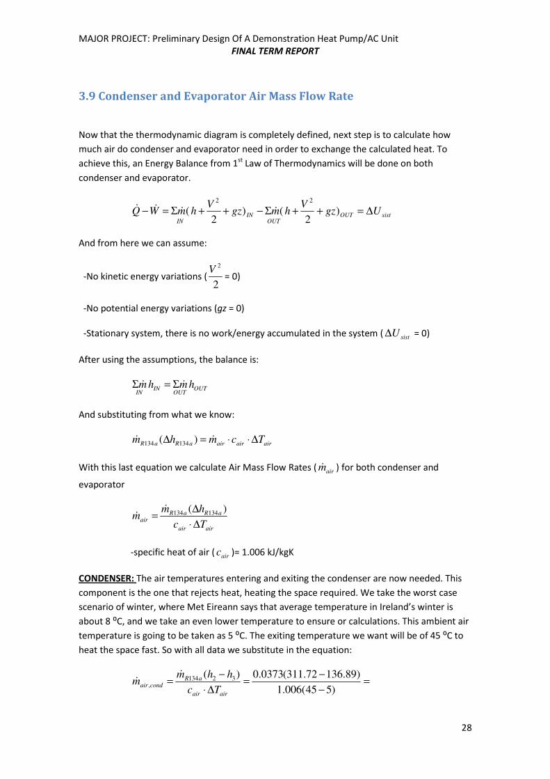
Both condenser and evaporator are going to be designed as cross-flow unmixed fluids heat

exchangers, where one fluid is R134-a refrigerant and the other one is air. Next figure is a

schematic explanation of both fluids movement. In the condenser refrigerant comes in hot and

cools down, affecting the air around it, that comes in cold and heats up. In the evaporator the

opposite process happens, where refrigerant comes in cold and heats up, affecting the air

around it, that comes in hot and cools down.

Figure 3.8. Cross-Flow heat exchanger (Refrigerant Fluid and Gas Flows)


FINAL TERM REPORT

30

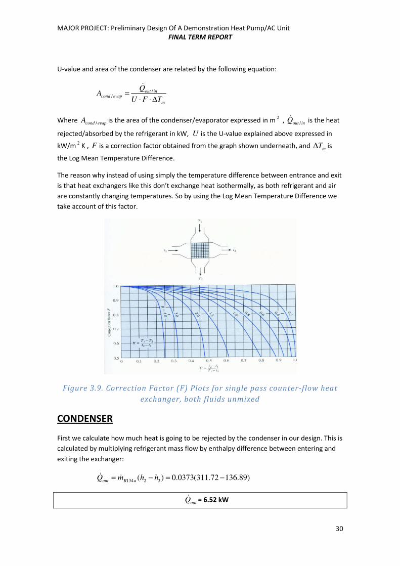
U-value and area of the condenser are related by the following equation:

m

inoutevapcond

TFU

QA

∆⋅⋅= /

/

&

Where evapcondA / is the area of the condenser/evaporator expressed in m2

, inoutQ /& is the heat

rejected/absorbed by the refrigerant in kW, U is the U-value explained above expressed in

kW/m2

K , F is a correction factor obtained from the graph shown underneath, and mT∆ is

the Log Mean Temperature Difference.

The reason why instead of using simply the temperature difference between entrance and exit

is that heat exchangers like this don’t exchange heat isothermally, as both refrigerant and air

are constantly changing temperatures. So by using the Log Mean Temperature Difference we

take account of this factor.

Figure 3.9. Correction Factor (F) Plots for single pass counter-flow heat

exchanger, both fluids unmixed

CONDENSER

First we calculate how much heat is going to be rejected by the condenser in our design. This is

calculated by multiplying refrigerant mass flow by enthalpy difference between entering and

exiting the exchanger:

)89.13672.311(0373.0)( 32134 −=−= hhmQ aRout&&

outQ& = 6.52 kW


FINAL TERM REPORT

31

This means that refrigerant rejects 6.52 kW of heating power in our system in order to heat

the intended space.

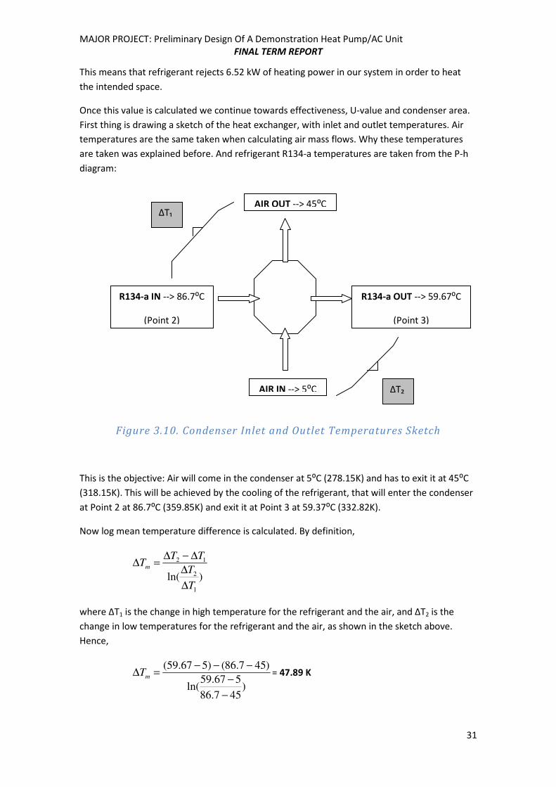
Once this value is calculated we continue towards effectiveness, U-value and condenser area.

First thing is drawing a sketch of the heat exchanger, with inlet and outlet temperatures. Air

temperatures are the same taken when calculating air mass flows. Why these temperatures

are taken was explained before. And refrigerant R134-a temperatures are taken from the P-h

diagram:

Figure 3.10. Condenser Inlet and Outlet Temperatures Sketch

This is the objective: Air will come in the condenser at 5⁰C (278.15K) and has to exit it at 45⁰C

(318.15K). This will be achieved by the cooling of the refrigerant, that will enter the condenser

at Point 2 at 86.7⁰C (359.85K) and exit it at Point 3 at 59.37⁰C (332.82K).

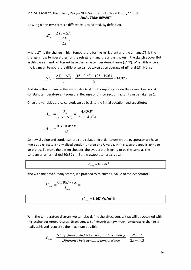
Now log mean temperature difference is calculated. By definition,

)ln(1

2

12

T

T

TTTm

∆

∆

∆−∆=∆

where ΔT1 is the change in high temperature for the refrigerant and the air, and ΔT2 is the

change in low temperatures for the refrigerant and the air, as shown in the sketch above.

Hence,

)457.86

567.59ln(

)457.86()567.59(

−

−

−−−=∆ mT = 47.89 K

R134-a IN --> 86.7⁰C

(Point 2)

AIR IN --> 5⁰C

AIR OUT --> 45⁰C

R134-a OUT --> 59.67⁰C

(Point 3)

ΔT₂

ΔT₁


FINAL TERM REPORT

32

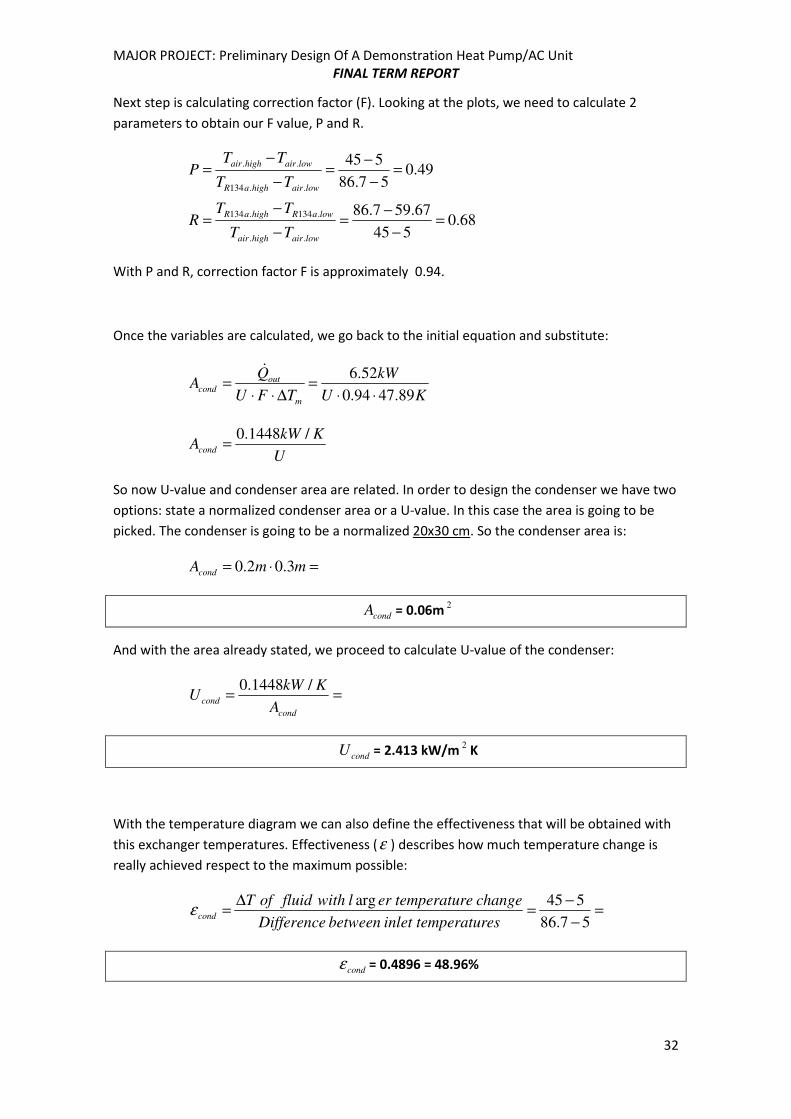
Next step is calculating correction factor (F). Looking at the plots, we need to calculate 2

parameters to obtain our F value, P and R.

68.0545

67.597.86

49.057.86

545

..

.134.134

..134

..

=−

−=

−

−=

=−

−=

−

−=

lowairhighair

lowaRhighaR

lowairhighaR

lowairhighair

TT

TTR

TT

TTP

With P and R, correction factor F is approximately 0.94.

Once the variables are calculated, we go back to the initial equation and substitute:

KU

kW

TFU

QA

m

outcond

89.4794.0

52.6

⋅⋅=

∆⋅⋅=

&

U

KkWAcond

/1448.0=

So now U-value and condenser area are related. In order to design the condenser we have two

options: state a normalized condenser area or a U-value. In this case the area is going to be

picked. The condenser is going to be a normalized 20x30 cm. So the condenser area is:

=⋅= mmAcond 3.02.0

condA = 0.06m2

And with the area already stated, we proceed to calculate U-value of the condenser:

==cond

condA

KkWU

/1448.0

condU = 2.413 kW/m2

K

With the temperature diagram we can also define the effectiveness that will be obtained with

this exchanger temperatures. Effectiveness (ε ) describes how much temperature change is

really achieved respect to the maximum possible:

=−

−=

∆=

57.86

545arg

estemperaturinletbetweenDifference

changeetemperaturerlwithfluidofTcondε

condε = 0.4896 = 48.96%


FINAL TERM REPORT

33

EVAPORATOR

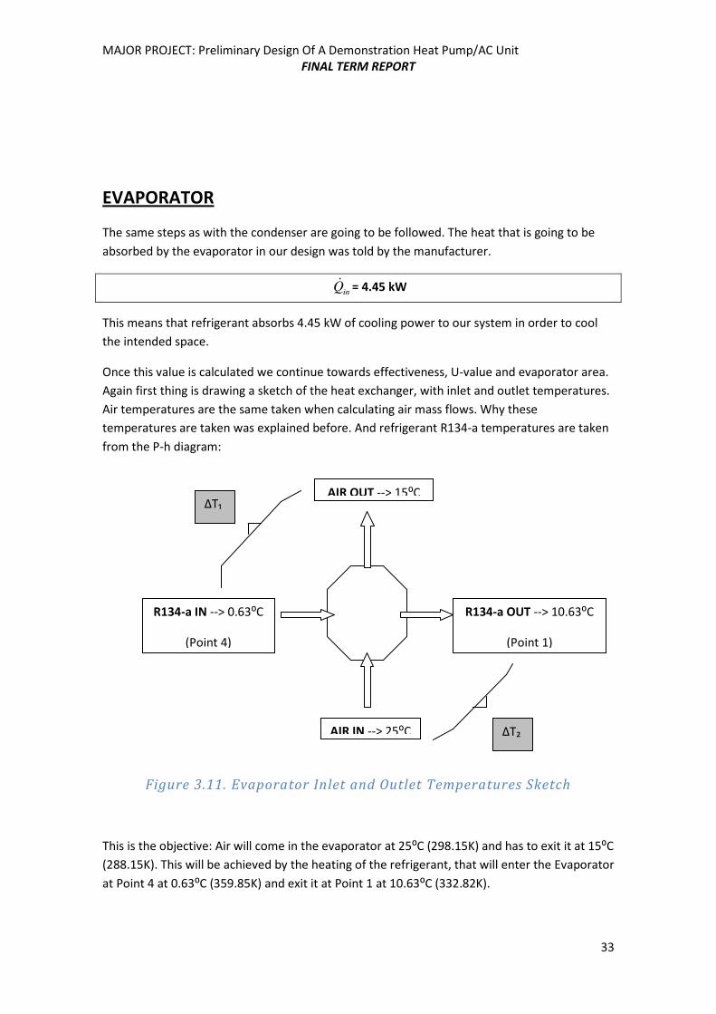
The same steps as with the condenser are going to be followed. The heat that is going to be

absorbed by the evaporator in our design was told by the manufacturer.

inQ& = 4.45 kW

This means that refrigerant absorbs 4.45 kW of cooling power to our system in order to cool

the intended space.

Once this value is calculated we continue towards effectiveness, U-value and evaporator area.

Again first thing is drawing a sketch of the heat exchanger, with inlet and outlet temperatures.

Air temperatures are the same taken when calculating air mass flows. Why these

temperatures are taken was explained before. And refrigerant R134-a temperatures are taken

from the P-h diagram:

Figure 3.11. Evaporator Inlet and Outlet Temperatures Sketch

This is the objective: Air will come in the evaporator at 25⁰C (298.15K) and has to exit it at 15⁰C

(288.15K). This will be achieved by the heating of the refrigerant, that will enter the Evaporator

at Point 4 at 0.63⁰C (359.85K) and exit it at Point 1 at 10.63⁰C (332.82K).

R134-a IN --> 0.63⁰C

(Point 4)

AIR IN --> 25⁰C

AIR OUT --> 15⁰C

R134-a OUT --> 10.63⁰C

(Point 1)

ΔT₂

ΔT₁


FINAL TERM REPORT

34

Now log mean temperature difference is calculated. By definition,

)ln(1

2

12

T

T

TTTm

∆

∆

∆−∆=∆

where ΔT1 is the change in high temperature for the refrigerant and the air, and ΔT2 is the

change in low temperatures for the refrigerant and the air, as shown in the sketch above. But

in this case air and refrigerant have the same temperature change (10⁰C). When this occurs,

the log mean temperature difference can be taken as an average of ΔT1 and ΔT2 .Hence,

2

)63.1025()63.015(

2

12 −+−=

∆+∆=∆

TTTm = 14.37 K

And since the process in the evaporator is almost completely inside the dome, it occurs at

constant temperature and pressure. Because of this correction factor F can be taken as 1.

Once the variables are calculated, we go back to the initial equation and substitute:

KU

kW

TFU

QA

m

inevap

37.141

45.4

⋅⋅=

∆⋅⋅=

&

U

KkWAcond

/310.0=

So now U-value and condenser area are related. In order to design the evaporator we have

two options: state a normalized condenser area or a U-value. In this case the area is going to

be picked. To make the design cheaper, the evaporator is going to be the same as the

condenser, a normalized 20x30 cm. So the evaporator area is again:

evapA = 0.06m2

And with the area already stated, we proceed to calculate U-value of the evaporator:

==evap

evapA

KkWU

/310.0

evapU = 5.167 kW/m2

K

With the temperature diagram we can also define the effectiveness that will be obtained with

this exchanger temperatures. Effectiveness (ε ) describes how much temperature change is

really achieved respect to the maximum possible:

=−

−=

∆=

63.025

1525arg

estemperaturinletbetweenDifference

changeetemperaturerlwithfluidofTevapε


FINAL TERM REPORT

35

evapε = 0.4103 = 41.03%

The following table resumes results obtained in this part:

CONDENSER EVAPORATOR

Dimensions Exchanger 20x30 cm 20x30 cm

U-value 2.413 kW/m2

K 5.167 kW/m2

K

Effectiveness 48.96% 41.03%

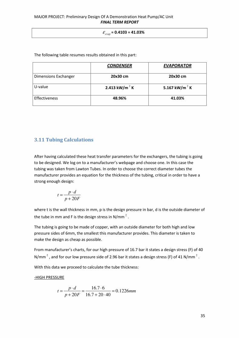
3.11 Tubing Calculations

After having calculated these heat transfer parameters for the exchangers, the tubing is going

to be designed. We log on to a manufacturer’s webpage and choose one. In this case the

tubing was taken from Lawton Tubes. In order to choose the correct diameter tubes the

manufacturer provides an equation for the thickness of the tubing, critical in order to have a

strong enough design:

Fp

dpt

20+

⋅=

where t is the wall thickness in mm, p is the design pressure in bar, d is the outside diameter of

the tube in mm and F is the design stress in N/mm2

.

The tubing is going to be made of copper, with an outside diameter for both high and low

pressure sides of 6mm, the smallest this manufacturer provides. This diameter is taken to

make the design as cheap as possible.

From manufacturer’s charts, for our high pressure of 16.7 bar it states a design stress (F) of 40

N/mm2

, and for our low pressure side of 2.96 bar it states a design stress (F) of 41 N/mm2

.

With this data we proceed to calculate the tube thickness:

-HIGH PRESSURE

mmFp

dpt 1226.0

40207.16

67.16

20=

⋅+

⋅=

+

⋅=


FINAL TERM REPORT

36

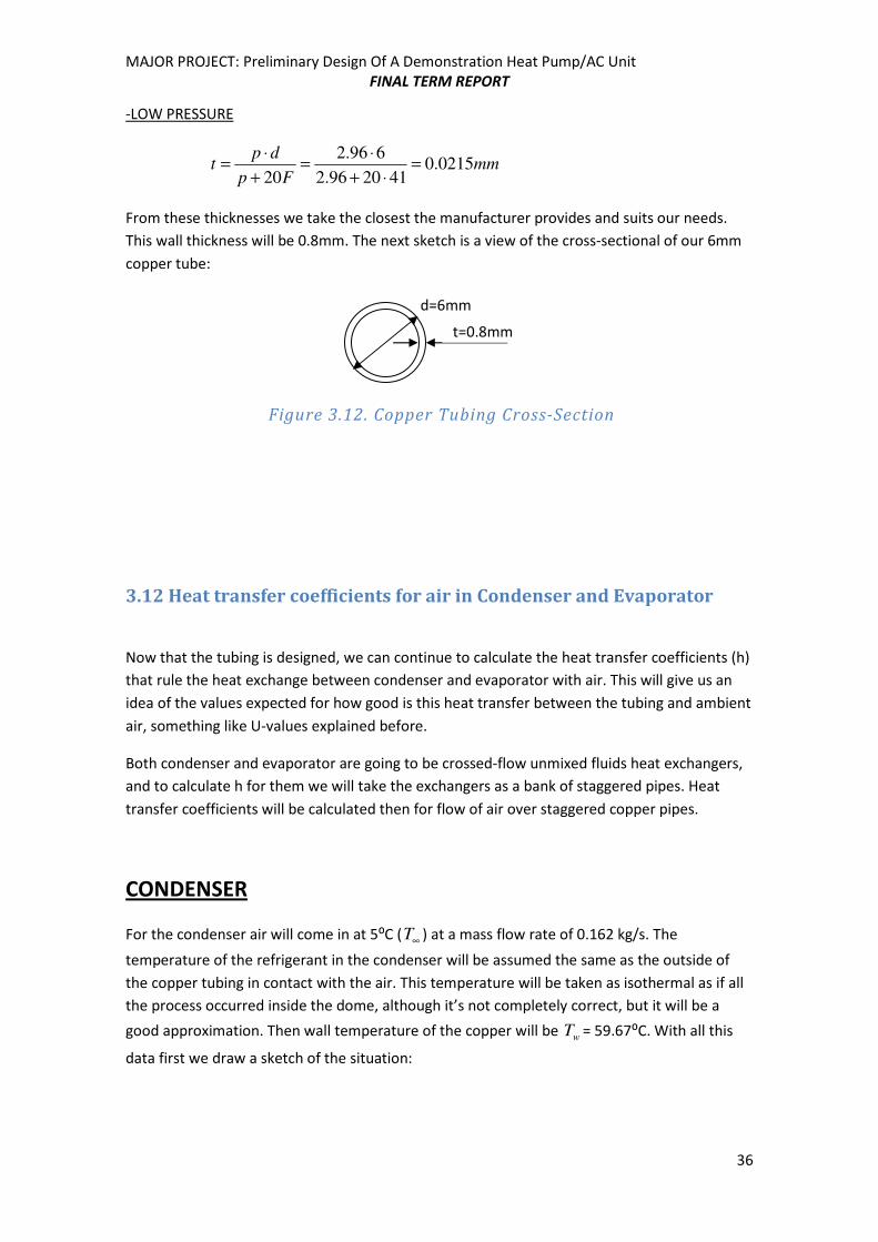
-LOW PRESSURE

mmFp

dpt 0215.0

412096.2

696.2

20=

⋅+

⋅=

+

⋅=

From these thicknesses we take the closest the manufacturer provides and suits our needs.

This wall thickness will be 0.8mm. The next sketch is a view of the cross-sectional of our 6mm

copper tube:

Figure 3.12. Copper Tubing Cross-Section

3.12 Heat transfer coefficients for air in Condenser and Evaporator

Now that the tubing is designed, we can continue to calculate the heat transfer coefficients (h)

that rule the heat exchange between condenser and evaporator with air. This will give us an

idea of the values expected for how good is this heat transfer between the tubing and ambient

air, something like U-values explained before.

Both condenser and evaporator are going to be crossed-flow unmixed fluids heat exchangers,

and to calculate h for them we will take the exchangers as a bank of staggered pipes. Heat

transfer coefficients will be calculated then for flow of air over staggered copper pipes.

CONDENSER

For the condenser air will come in at 5⁰C ( ∞T ) at a mass flow rate of 0.162 kg/s. The

temperature of the refrigerant in the condenser will be assumed the same as the outside of

the copper tubing in contact with the air. This temperature will be taken as isothermal as if all

the process occurred inside the dome, although it’s not completely correct, but it will be a

good approximation. Then wall temperature of the copper will be wT = 59.67⁰C. With all this

data first we draw a sketch of the situation:

d=6mm

t=0.8mm


FINAL TERM REPORT

37

condairm ,& =0.162 kg/s

∞T = 5⁰C

Figure 3.13. Condenser Modelled as Air Flow over Staggered Pipes

With this clear, calculations can be done. From empirical correlations it can be estimated that

for air flow over staggered banks of pipes:

6.0Re33.0 ⋅⋅= hCNu

where Nu is Nusselt Number, a non-dimensional number proportional to h, hC is a correction

factor equal to 1.1 for staggered pipes, and Re is Reynolds Number, another non-dimensional

number that takes account of the kinetic factor affecting the fluid.

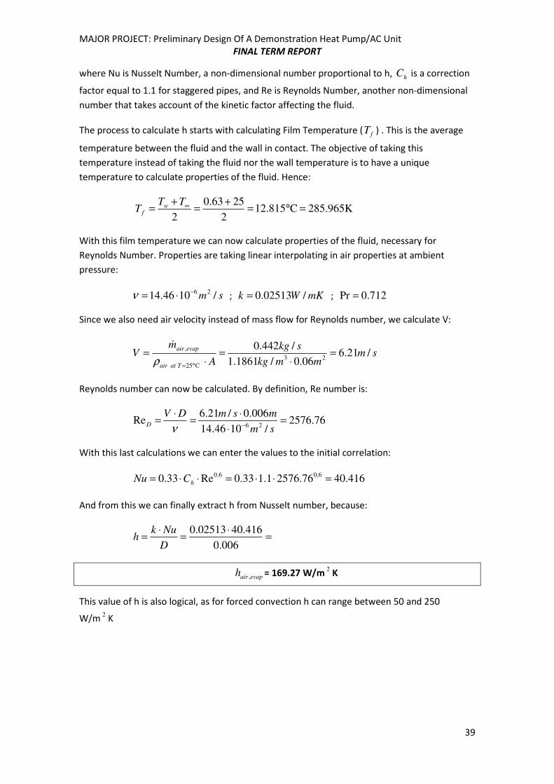
The process to calculate h starts with calculating Film Temperature ( fT ) . This is the average

temperature between the fluid and the wall in contact. The objective of taking this

temperature instead of taking the fluid nor the wall temperature is to have a unique

temperature to calculate properties of the fluid. Hence:

305.485K C335.322

567.59

2=°=

+=

+= ∞TT

T wf

With this film temperature we can now calculate properties of the fluid, necessary for

Reynolds Number. Properties are taking linear interpolating in air properties at ambient

pressure:

sm /1025.16 26−⋅=ν ; mKWk /02666.0= ; 707.0Pr =

Since we also need air velocity instead of mass flow for Reynolds number, we calculate V:

smmmkg

skg

A

mV

Tatair

condair/11.2

06.0/2803.1

/162.023

C5

,=

⋅=

⋅=

°=ρ

&

Reynolds number can now be calculated. By definition, Re number is:

08.779/1025.16

006.0/11.2Re

26=

⋅

⋅=

⋅=

− sm

msmDVD

ν

R134-a

wT = 59.67⁰C


FINAL TERM REPORT

38

With these last calculations we can enter the values to the initial correlation:

718.1908.7791.133.0Re33.0 6.06.0 =⋅⋅=⋅⋅= hCNu

And from this we can finally extract h from Nusselt number, because:

=⋅

=⋅

=006.0

718.1902666.0

D

Nukh

condairh , = 86.61 W/m2

K

This value of h is logical, as for forced convection h can range between 50 and 250 W/m2

K

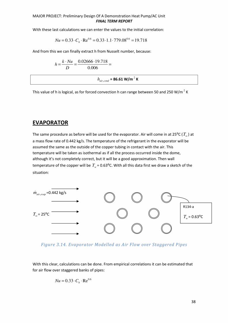
EVAPORATOR

The same procedure as before will be used for the evaporator. Air will come in at 25⁰C ( ∞T ) at

a mass flow rate of 0.442 kg/s. The temperature of the refrigerant in the evaporator will be

assumed the same as the outside of the copper tubing in contact with the air. This

temperature will be taken as isothermal as if all the process occurred inside the dome,

although it’s not completely correct, but it will be a good approximation. Then wall

temperature of the copper will be wT = 0.63⁰C. With all this data first we draw a sketch of the

situation:

evapairm ,& =0.442 kg/s

∞T = 25⁰C

Figure 3.14. Evaporator Modelled as Air Flow over Staggered Pipes

With this clear, calculations can be done. From empirical correlations it can be estimated that

for air flow over staggered banks of pipes:

6.0Re33.0 ⋅⋅= hCNu

R134-a

wT = 0.63⁰C


FINAL TERM REPORT

39

where Nu is Nusselt Number, a non-dimensional number proportional to h, hC is a correction

factor equal to 1.1 for staggered pipes, and Re is Reynolds Number, another non-dimensional

number that takes account of the kinetic factor affecting the fluid.

The process to calculate h starts with calculating Film Temperature ( fT ) . This is the average

temperature between the fluid and the wall in contact. The objective of taking this

temperature instead of taking the fluid nor the wall temperature is to have a unique

temperature to calculate properties of the fluid. Hence:

285.965K C815.122

2563.0

2=°=

+=

+= ∞TT

T wf

With this film temperature we can now calculate properties of the fluid, necessary for

Reynolds Number. Properties are taking linear interpolating in air properties at ambient

pressure:

sm /1046.14 26−⋅=ν ; mKWk /02513.0= ; 712.0Pr =

Since we also need air velocity instead of mass flow for Reynolds number, we calculate V:

smmmkg

skg

A

mV

Tatair

evapair/21.6

06.0/1861.1

/442.023

C25

,=

⋅=

⋅=

°=ρ

&

Reynolds number can now be calculated. By definition, Re number is:

76.2576/1046.14

006.0/21.6Re

26=

⋅

⋅=

⋅=

− sm

msmDVD

ν

With this last calculations we can enter the values to the initial correlation:

416.4076.25761.133.0Re33.0 6.06.0 =⋅⋅=⋅⋅= hCNu

And from this we can finally extract h from Nusselt number, because:

=⋅

=⋅

=006.0

416.4002513.0

D

Nukh

evapairh , = 169.27 W/m2

K

This value of h is also logical, as for forced convection h can range between 50 and 250

W/m2

K


FINAL TERM REPORT

40

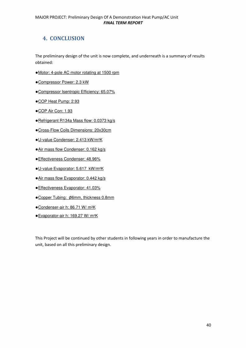
4. CONCLUSION

The preliminary design of the unit is now complete, and underneath is a summary of results

obtained:

�Motor: 4-pole AC motor rotating at 1500 rpm �Compressor Power: 2.3 kW

�Compressor Isentropic Efficiency: 65.07%

�COP Heat Pump: 2.93

�COP Air Con: 1.93

�Refrigerant R134a Mass flow: 0.0373 kg/s

�Cross-Flow Coils Dimensions: 20x30cm

�U-value Condenser: 2.413 kW/m2K

�Air mass flow Condenser: 0.162 kg/s

�Effectiveness Condenser: 48.96%

�U-value Evaporator: 5.617 kW/m2K

�Air mass flow Evaporator: 0.442 kg/s

�Effectiveness Evaporator: 41.03%

�Copper Tubing: Ø6mm, thickness 0.8mm

�Condenser-air h: 86.71 W/ m2K

�Evaporator-air h: 169.27 W/ m2K

This Project will be continued by other students in following years in order to manufacture the

unit, based on all this preliminary design.


FINAL TERM REPORT

41

5. BIBLIOGRAPHY

Professor Oliver Mulryan (GMIT, Galway, Ireland): “Notes for Thermodynamics”

Moran& Shapiro: “Fundamentals of Engineering Thermodynamics”, 5th Edition

http://www.learnthermo.com

http://www.wikipedia.org

http://www.autodata.com

http://china-heatpipe.net/heatpipe04/08/2008-4-24/The_Vapor-

Compression_Refrigeration_Cycle.htm

http://www.refrigerationbasics.com

http://www.met.ie/

http://www.lawtontubes.co.uk/refrigeration.htm

Date post:	05-Apr-2022
Category:	Documents
Upload:	others
View:	3 times
Download:	0 times

Preliminary Design of a Demonstration Heat Pump/AC Unit

Documents