Preliminary results of the Fp7 project CoBiOS Coastal...

Liege colloquium 9-5-2012

Harmonization of Ocean Colour products

GMES downstream services Project number: 263295 Duration: 1-1-2011 - 31-12-2013 [email protected] +31 20 598 9547

Preliminary results of the

Fp7 project CoBiOS

Coastal Biomass Observatory

Services

www.cobios.eu

Steef Peters (VU-IVM + Water Insight)

With contributions from

Marieke Eleveld (VU-IVM)

Carole Lebreton (Brockmann Consult)

Kerstin Stelzer (Brockmann Consult)

Stefan Simis (Syke)

Jenni Attilla (Syke)

Seppo Kaitala (Syke)

Hanna Alasalmi (Syke)

Mikko Kervinen (Syke)

Lars Boye Hansen (GRAS)

Kees van Ruiten (Deltares)

Kathrin Poser (Water Insight)

mailto:[email protected]

http://www.cobios.eu/


What is the CoBiOS project?

CoBiOS aims to integrate satellite products and ecological models into a really operational

and user-relevant information service on high biomass blooms in Europe’s coastal

waters.

3 Key elements:

1) EO-products (operational algorithms)

(based on MERIS satellite images:

Chl-a and transparency)

2) Ecological models and

3) The service portal

EO-products

(outputs)

Model

Inputs & outputs

Services

Portal

The idea is:

1) To improve eco-hydrological models by driving them with satellite-derived Kd

2) To locate high biomass events using satellite data

3) To predict the fate of high biomass events using the improved models

4) To derive meaningfull statistics from ensembles of model runs and EO-results


Why ensemble EO-products?

An example from operational water level prediction models

K. Van Ruiten Deltares

Figure 1. NOOS Near Real Time Forecast product: Water Level, based on the ensemble of results from

several models together with the observed value (black line)


Why ensemble EO-products?

Reducing prediction uncertainty will lead to better event probability estimation

K. Van Ruiten, Deltares

Causality chain from prediction (forecast) to management action / procedure

EO-data

+

Models

Is there a high

biomass bloom?

will it move towards

a mushel farm?

If more algorithms

predict a high biomass bloom

then the probability is higher

that it is really there

If the prediction is

better, a better choice

can be made

between measures


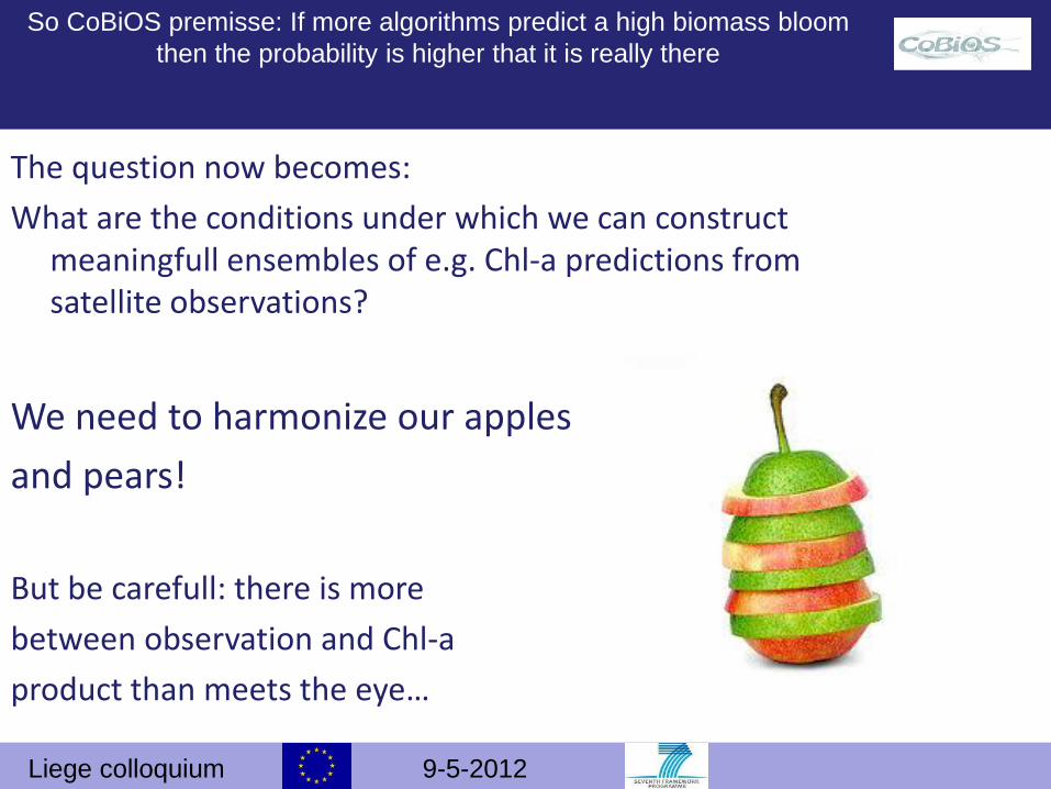
The question now becomes:

What are the conditions under which we can construct meaningfull ensembles of e.g. Chl-a predictions from satellite observations?

We need to harmonize our apples

and pears!

But be carefull: there is more

between observation and Chl-a

product than meets the eye…

So CoBiOS premisse: If more algorithms predict a high biomass bloom

then the probability is higher that it is really there


L1 input data

L1 to L2 processsing

L2 reflectance data + ancillary data

L2 to Water quality products processing

Water Quality products per image

L3 selection and aggregation

Aggregated information products

Wa

ter

Insi

gh

t P

roce

ssin

g c

ha

in f

or

Me

dite

rra

ne

an

ME

RIS

im

ag

es

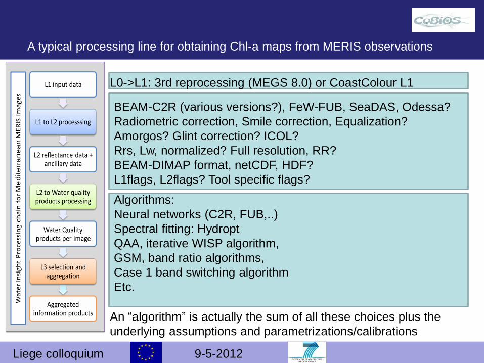
A typical processing line for obtaining Chl-a maps from MERIS observations

L0->L1: 3rd reprocessing (MEGS 8.0) or CoastColour L1

BEAM-C2R (various versions?), FeW-FUB, SeaDAS, Odessa?

Radiometric correction, Smile correction, Equalization?

Amorgos? Glint correction? ICOL?

Rrs, Lw, normalized? Full resolution, RR?

BEAM-DIMAP format, netCDF, HDF?

L1flags, L2flags? Tool specific flags?

Algorithms:

Neural networks (C2R, FUB,..)

Spectral fitting: Hydropt

QAA, iterative WISP algorithm,

GSM, band ratio algorithms,

Case 1 band switching algorithm

Etc.

An “algorithm” is actually the sum of all these choices plus the

underlying assumptions and parametrizations/calibrations


-Harmonization of formats and tools where possible

-Use a single L1 starting point (3rd reprocessing);

-Apply radiometric correction, smile correction & Equalization

-Not glint correction; Not ICOL adjacency correction

-Use the best atmospheric correction for a certain area (C2R

or FuB)

-Use as much as possible the same flags for pixel selection

-Use well documented and understood operational algorithms

-Document the calibration/validation of algorithms if possible

-Pay close attention to the local validity of algorithms ->

Change the parameterization for other areas if possible

CoBiOS choices on the road to harmonization of EO-products


Operational algorithms used in the project so far:

IVM HYDROPT Hydrolight lookup table Calibrated for North Sea

can be adapted to other SIOPs

WI predictor-corrector algorithm Calibrated on Nomad and Hydrolight simulations

Can be adapted to other SIOPs

GRAS C2R_DK adapted neural network Calibrated using field observations

Can be adapted to different Chl-a regimes

BC C2R standard neural network Calibrated on North Sea data?

Can be adapted by retraining or

by changing coeffients

BC FUB standard other neural network Calibrated on Baltic Sea data

BC QAA (CC processor) quasi analytical band ratio Calibrated on NOMAD data

IPF L2 standard 3rd slightly different neural network Calibration?

MyOcean Empirical algorithm Calibrated on global data

A closer look at the algorithms (to derive Chl-a from MERIS Rrs)


Accuracy of std MERIS & HYDROPT products.

A

In Situ Chla (mgm-3)

0.1 1 10 100

ME

RIS

AP

2 (

mg m

-3)

0.1

1

10

100MERIS AP2 Chlalog(Y) = log(x)0.69 + 0.078; r2 = 0.51; N = 61.

B

In Situ Chla (mgm-3)

0.1 1 10 100H

YD

RO

PT

Chla

(m

g m

-3)

0.1

1

10

100HYDROPT sIOP Chla

log(Y) = log(x)0.84 + 0.02; r2 = 0.88; N = 61.

C

In Situ TSM (g m-3)

0.1 1 10 100

ME

RIS

TS

M (

g m

-3)

0.1

1

10

100

D

In Situ TSM (g m-3)

0.1 1 10 100

HY

DR

OP

T T

SM

(g m

-3)

0.1

1

10

100 HYDROPT sIOP TSM

log(Y) = log(x)0.94 - 0.10; r2 = 0.67; N = 52.

MERIS TSM log(Y) = log(x)0.87 - 0.11; r2 = 0.74; N = 52.

HYDROPT sIOP aCDOM

log(Y) = log(x)0.90 - 0.09; r2 = 0.70; N = 15.

In Situ aCDOM

(442) (m-1)

0.001 0.01 0.1 1 10

HY

DR

OP

T a

CD

OM

(442)

(m-1

)

0.001

0.01

0.1

1

10MERIS adg

log(Y) = log(x)0.87 - 0.32; r2 = 0.43; N = 15.

In Situ adg

(442) (m-1)

0.001 0.01 0.1 1 10

ME

RIS

ad

g (

442)

(m-1

)

0.001

0.01

0.1

1

10

E F Tilstone et al. Remote Sensing of Environment

118

1. MERIS standard Case 2 product (AP2):a neural network (NN) that derives a and b and through empirical

relationships, it converts IOP to Chla and TSM concentrations.

2. HYDROPT parameterised with sIOP (HYD):Semi-analytical algorithm that combines the approach of Garver

and Siegel [1997] with the radiative transfer code HYDROLIGHT

[Mobley, 1994] to partition the reflectance spectra into its

respective IOP. It predicts remote sensing reflectance spectrum

from knowledge of the sIOP of a particular region and retrieves the

concentrations by minimizing the difference between observed and

modeled reflectance spectra.

M S Log-RMS Rel %

AP2 Chla -0.06 0.25 0.26 40

HYDChla -0.08 0.15 0.17 9

AP2 TSM -0.22 0.24 0.33 33

HYDTSM -0.14 0.31 0.34 50

AP2adg -0.24 0.51 0.58 19

HYDcdom 0.11 0.28 0.31 13


Assumptions of the WI algorithm

Remote sensing reflectance

Model according to Park&Ruddick

(2005)

The WI algorithm solves the 4th degree Park&Ruddick polynomial

equation using a predictor-corrector iterative approach


The WI algorithm: some validation results: NOMAD

10-1

100

101

10-1

100

101

Comparison NOMAD - WISP Algorithm

Chl-a NOMAD HPLC

Chl-a r

esults W

ISP

Alg

orith

m

Chl-a

Suspect

r2 = 0.74141

slope = 0.87642

intercept = 0.15956

rmse = 0.32337

n = 176

10-2

10-1

10-2

10-1

Comparison NOMAD - WISP Algorithm

CDOM NOMAD

CD

OM

results W

ISP

Alg

orith

m

CDOM

Suspect

r2 = 0.74141

slope = 0.87642

intercept = 0.15956

rmse = 0.32337

n = 176

r2 = 0.72909

slope = 0.97011

intercept = -0.13693

rmse = 0.25868

n = 151


The CoBiOS experiment


North Sea & WEC: Chla, TSM and CDOM.

A

Chla (mg m-3

)0 5 10 15 20 25

E

TSM (g m-3

)0 5 10 15 20

Skagerrak

NW North Sea

East Anglia

NE North Sea

German Bight

Dutch Coast

West Jutland

Belgium Coast

WEC

Celtic Sea

D

aCDOM

(m-1

)

0.0 0.2 0.4 0.6 0.8 1.0 1.2

Skagerrak

NW North Sea

East Anglia

NE North Sea

German Bight

Dutch Coast

West Jutland

Belgium Coast

WEC

Celtic Sea

Tilstone et al.

Remote sensing of

environment 118

Chla varied from 0.23 to 35 mg m-3 was significantly

higher along the Dutch Coast lowest in WEC and NW

North Sea.

TSM varied from 0.2 to 75.5 g m-3 higher along the

German Bight, Belgium and Dutch coasts and lowest

in the WEC and Celtic Sea.

aCDOM(442) varied from 0.02 to 2.16 m-1, was highest

in the Skagerrak, German Bight and lowest in the

Celtic sea.


Many challenges:

•Shallow

•Eutrophic

•Salinity gradient

•Limited exchange

•Permanent halocline

•Seasonal thermocline

•Big rivers

•Shipping

Mainly absoption by

Phytoplankton and CDOM

Very little TSM

The CoBiOS experiment: The Baltic Sea

Origin: S. Simis; SYKE


North Sea Collocated `Chl-a: results Origin: C. Lebreton + K. Stelzer (BC)


North Sea Collocated

`Chl-a: results Origin: C.

Lebreton + K. Stelzer

(BC)


Origin: C. Lebreton + K. Stelzer (BC)





Preliminary conclusions

•The ensemble approach seems promising

•It provides insight in the relative spatial distributions of various algorithms

•The ensemble mean is approaching the in-situ data and following the variability in

the in-situ data

•We can clearly identify which algorithms are out of range and should have local

tuning

•Some algorithms have different spatial patterns from Chl-a to CDOM

•The ensemble may be biased by too many versions of the same neural network

•A probability of bloom occurence based on these operational algorithms seems

feasible

Next steps:

Implement various Kd algorithms (PAR)

Implement further ensemble statistics

Do final tests and go the operational phase

BUT: MERIS? MODIS?.....Sentinel 3

Acknowledgements

The research leading to these results has received funding from the

European Community's Seventh Framework Programme ([FP7/2007-

2013]) under grant agreement n° 263295

Especially the CoBiOS teams at Brockmann Consult, IVM, SYKE, WI

and GRAS are gratefully acknowledged

THANK YOU!

Date post:	17-Mar-2018
Category:	Documents
Upload:	lethuan
View:	214 times
Download:	1 times

Preliminary results of the Fp7 project CoBiOS Coastal...

Documents