188
premio tesi di dottorato – 25 –

premio tesi di dottorato
– 25 –

Premio Tesi di doTToraTo Panel of Judges, year 2011
Luigi Lotti, Faculty of Political Sciences (Panel Chairman)
Tito arecchi, Faculty of Mathematical, Physical and Natural SciencesPaolo Felli, Faculty of Architecturemichele arcangelo Feo, Faculty of Arts and Philosophyroberto Genesio, Faculty of Engineeringmario Pio marzocchi, Faculty of Pharmacysalvo mastellone, Faculty of Education and Training SciencesLuciano mecacci, Faculty of Psychologyadolfo Pazzagli, Faculty of Medicine and Surgerymario Giuseppe rossi, Faculty of Arts and Philosophysalvatore ruggieri, Faculty of Medicine and SurgeryPiero Tani, Faculty of EconomicsFranco scaramuzzi, Faculty of AgricultureFiorenzo Cesare Ugolini, Faculty of AgricultureVincenzo Varano, Faculty of Law

Nicole Fabbri
Bragg spectroscopy of quantum gases
exploring physics in one dimension
Firenze University Press2012

Bragg spectroscopy of quantum gases: exploring physics in one dimension / Nicole Fabbri. – Firenze : Firenze University Press, 2012.(Premio FUP. Tesi di dottorato ; 25)
http://digital.casalini.it/9788866552215
isBN 978-88-6655-220-8 (print)isBN 978-88-6655-221-5 (online)
Peer Review Processall publications are submitted to an external refereeing process under the responsibility of the FUP editorial Board and the scientific Committees of the individual series. The works published in the FUP catalogue are evaluated and approved by the editorial Board of the publishing house. For a more detailed description of the refereeing process we refer to the official documents published on the website and in the online catalogue of the FUP (http://www.fupress.com).Firenze University Press Editorial BoardG. Nigro (Co-ordinator), m.T. Bartoli, m. Boddi, F. Cambi, r. Casalbuoni, C. Ciappei, r. del Punta, a. dolfi, V. Fargion, s. Ferrone, m. Garzaniti, P. Guarnieri, G. mari, m. marini, m. Verga, a. Zorzi.
© 2012 Firenze University PressUniversità degli studi di FirenzeFirenze University PressBorgo albizi, 28, 50122 Firenze, italyhttp://www.fupress.com/Printed in Italy
Graphic design alberto Pizarro Fernández, Pagina maestra snc
Contents
Introduction 1 Chapter 1 One dimensional systems: Luttinger liquids and Mott transition 7 1.1 One-dimensional systems 8 1.2 Luttinger liquids 9 1.2.1 The Hamiltonian 10 1.2.2 Regimes of interaction 11 1.3 One-dimensional Bose gases 13 1.3.1 Lieb-Liniger model 14 1.3.2 Regimes of degeneracy in a trapped 1D gas 16 1.4 Interacting bosons in a lattice 19 1.4.1 The microscopic model: Bose-Hubbard 20 1.4.2 Superfluid and Mott insulator states 22 Chapter 2 Experimental realization 27 2.1 Driving atoms to quantum degeneracy 28 2.1.1 Observing atoms after a TOF 32 2.2 Optical lattices: Manipulating atoms with light 36 2.2.1 Light as an optical potential for atoms 36 2.2.2 Optical lattices: A periodic potential 40 2.2.2.1 Experimental realization 43 2.2.3 Adiabatically loading atoms into a lattice potential 46 2.3 Realizing an array of 1D gases 48 2.3.1 Atom distribution in the array 48 2.3.2 Some numbers for our 1D gases 54 2.4 Realizing the superfluid-to-insulator transition 57 2.4.1 Momentum distribution across the transition 58 2.5 Conclusions 60
Nicole Fabbri, Bragg spectroscopy of quantum gases: Exploring physics in one dimension isBN 978-88-6655-220-8 (print) isBN 978-88-6655-221-5 (online) © 2012 Firenze University Press
Nicole Fabbri
VI
Chapter 3 Spectroscopy via inelastic light scattering 61 3.1 Generalities about Bragg scattering 61 3.1.1 Diffracting atoms at rest off a moving lattice 63 3.1.2 Two-photon Bragg transition 64 3.2 Information on low-energy excitations 66 3.2.1 Measure polarizability 66 3.2.2 Low-energy excitations 68 3.2.3 Low-energy excitations in a lattice-gas 69 3.3 Bragg setup 72 3.3.1 Calibration of the momentum transfer 74 3.3.2 Experimental procedure 76 3.4 Probe the excitations of the system 78 3.4.1 How to relate the experimental observable to energy absorption 78 3.4.2 Amount of excitations 80 3.4.3 Linear response 82 3.5 Conclusions 83 Chapter 4 Thermal phase-fluctuations in one dimension 85 4.1 Introduction 85 4.1.1 The experiment 87 4.2 Investigate coherence via Bragg scattering 89 4.2.1 Momentum distribution dominated by phase-fluctuations 93 4.2.2 Effective coherence length 94 4.3 Direct imaging of momentum distribution 96 4.4 Simulating the response of the array 100 4.5 Measure Temperature 104 4.6 Conclusions 105 Chapter 5 Exploring the superfluid-to-insulator transition in a lattice 107 5.1 Does Bragg scattering tell something more on Mott insulators? 108 5.1.1 The experiment 109 5.2 Characterizing the Superfluid-to-Insulator transition 112 5.3 Correlated superfluid in the lowest band 116 5.4 Response of an inhomogeneous Mott insulator 121 5.4.1 Gapped excitations of Mott islands 122 5.4.2 Lower-frequency response 127
Nicole FabbriVi
Contents
VII
5.5 Conclusions 130 Chapter 6 Inter-band spectroscopy in a lattice 133 6.1 A 3D BEC in a periodic potential 134 6.1.1 Comparison with Bogoliubov bands 137 6.1.2 Band mapping of a 3D BEC in a lattice 140 6.2 Inter-band spectroscopy of Mott states 141 6.2.1 Multi-band spectrum of a Mott insulating state 144 6.2.2 Band population of the Mott insulating states 145 6.2.3 Towards novel information about the Mott state 147 6.3 Conclusions 152 Outlook and prospects 153 Appendixes Rubidium atom and lasers for producing Bose-Einstein condensates 159 A.1 87-Rubidium 159 A.2 Laser light for producing BEC 157 Acknowledgements 163 Bibliography 165 Publications 177
ViiContents


Introduction
One-dimensional systems are a fertile ground for studying the physics of quantum many-body systems with strong correlations and fluctuations. They are among the most intriguing physical problems, since no simple picture captures their behaviour. In a three-dimensional world, one dimension is not a bare abstraction, but finds many realizations: A large amount of research work in the last twenty years has been devoted to implementing and studying them, within different fields of physics. From the 90's, progress in material science allowed for finding bulk materials exhibiting very anisotropic magnetic and electronic properties which reveal a one-dimensional structure inside. Remarkable examples of that are organic conductors [1, 2, 3, 4, 5], as well as spin [6, 7] and ladder compounds [8, 9]. In the same years, an impressive boost in chemical synthesis and nanotechnologies brought to the realization of iso-lated one-dimensional systems, where electrons are confined to move along one or a few conduction channels. Examples of this class are quantum wires [10, 11], Joseph-son junction arrays [12], edge states in quantum Hall systems [13], and nanotubes [14, 15]. Their physics drastically differs from the usual physics of interacting parti-cles, that is, the one known in higher dimensions. A plethora of quantum effects arises, such as field-induced spin density waves, ordered states like the spin-Peierls, and, last but not least, superconducting states. Yet, although many realizations have been implemented and a great amount of work has been already done, a complete de-scription of the phenomena occurring in these systems is hardly attainable, due to their complexity, and many questions still have to be addressed.
On this prospect, new possibilities have been opened by the realization of ultra-cold gases in degenerate quantum states and by the development of techniques to manipulate them in light-induced periodic potential, the so-called optical lattices. As a matter of fact, quite surprisingly, gases can realize interactions-induced strongly-correlated systems in an unprecedented way. This is in contrast to the common ex-perience whereby strong correlations only concerns solids or liquids, whereas gases are presumed to be weakly interacting by definition. Ultracold gases even present some important advantages compared to the alternative realizations of condensed-matter physics. For example, it is possible to apply forces much stronger than electric forces usually imposed on electrons in crystalline solids. It is possible to switch the
Nicole Fabbri, Bragg spectroscopy of quantum gases: Exploring physics in one dimension isBN 978-88-6655-220-8 (print) isBN 978-88-6655-221-5 (online) © 2012 Firenze University Press

Nicole Fabbri
2
potential on and off abruptly, as well as to modulate it. Besides, optical lattices pro-vide an effective tool for tuning the atom-atom interactions, since the depth of the periodic potential can be easily modified by changing frequency and intensity of the laser light producing the lattice. This is a fundamental point, especially concerning the realization of one-dimensional systems, because it makes possible to strictly com-pare experiment and theory, which is more difficult for the other realizations.
The starting point of this adventure was the achievement of Bose-Einstein con-densation in ultracold dilute gases, in 1995 [16, 17]. This accomplishment has opened a new Chapter in atomic and molecular physics, the core of which is given by particle statistics and interactions, rather than single-atom behaviour. The Bose-Einstein condensate (BEC) is described by a coherent, macroscopic matter-wave in an inter-acting many-body system, similar to what occurs in superconductivity and sperfluid-ity. Therefore, the many-body aspect of a BEC is reduced to an effective single-particle description. Actually, optical lattices were introduced slightly before the achievement of Bose-Einstein condensation. For a few years, they became a prime tool for exploring a wide range of phenomena associated with the existence of coher-ent matter-waves, such as Bloch oscillations [18] and atom diffraction [19, 20, 21, 22, 23]. Spatial ordering of the atoms in the lattices was demonstrated [24]. Optical lat-tices were also used to improve atom laser-cooling through resolved-sideband Raman laser cooling [25, 26]. Nevertheless, at this stage many-body physics was still unfeasi-ble due to the too high temperatures and the too low densities of the atomic samples. The true turning point for the study of many-body problems came from the combi-nation of optical lattices and Bose-Einstein condensates.
First experiments demonstrated the superfluid behaviour of BECs in optical lat-tices [27, 28, 29], e.g., emulating the physics of arrays of Josephson junctions [30]. At the same time, experiments started to realize complex many-body states, relevant for simulating condensed-matter systems, first with BECs [31, 32, 33, 34, 35], and later with ultracold Fermi gases [36, 37]. Strongly-confining optical lattices have been used to create microtraps for the atoms, the geometry of which can be appositely chosen to produce one-dimensional bosonic systems [32, 33, 34]. Thus, we can say that optical lattices have provided the equivalent of the lithography processes for trapping fer-mions in quantum wires or the chemical mechanisms bringing the formation of nanotubes in one-dimensional organic materials. This has allowed exploring new re-gimes. Whereas in a three-dimensional gas interactions can be neglected or effec-tively described in terms of noninteracting quasi-particles, e.g., in the framework of the Bogoliubov-De Gennes perturbation theory [38], in one-dimension interactions can become so strong that the Bogoliubov-like theories fail [39]. This occurs espe-cially at very low densities. Besides, as mentioned before, optical lattices allow for tuning the strength of the interatomic interactions compared to the kinetic energy of the gas [40], in an alternative manner to Feshbach resonances [41, 42]: In this way,
Nicole Fabbri2

Introduction
3
the interaction-induced transition from a superfluid state to a Mott insulator state has been observed [31, 32].
Thus, ultracold gases in optical lattices can be a favourable test-ground for realiz-ing and manipulating strongly correlated quantum phases and approaching many physical problems [43]. In addition, they constitute a promising candidate for im-plementing quantum information processing and quantum simulation schemes [44]. To achieve these goals, a corner stone consists in a precise characterization of the cor-related gaseous phases.
As in solid-state physics, experimental tools are necessary to characterize these quantum many-body ultracold gases. A natural candidate is the study of the response to scattering processes, in a similar manner to what is done in condensed-matter physics. Along those lines several techniques have been proposed in the latest years, consisting in scattering photons from the correlated atomic state, and some of them have been implemented recently. They include radio-frequency spectroscopy [45, 46], Raman spectroscopy [47] and Bragg spectroscopy [48, 49, 50, 52, 51].
This thesis
The PhD thesis presented here is part of the context described above. It was carried out at the European Laboratory for Non-linear Spectroscopy (LENS) in Florence, with the partnership of Universidad Complutense de Madrid, and consisted of three years of work performed in the group of Quantum Degenerate Gases directed by Prof. Massimo Inguscio. The experiments I will describe were realized on the appara-tus of the laboratory ‘BEC1’, under the supervision of Dr. Chiara Fort. The core ap-paratus, implemented for producing quantum degenerate Bose-Einstein condensates of Rubidium-87, has been working since 1998.
In order to explore the physics of one-dimensional systems, the Bose-Einstein condensate has been trapped in an array of one-dimensional gases in different quan-tum regimes by exploiting strongly-confining optical lattices. For characterizing these quantum phases, we mainly exploited inelastic light scattering (referred to as Bragg spectroscopy). This technique provides a tool which weakly perturbs the system, and creates excitations with independently tuneable momentum and energy. Thus, via Bragg spectroscopy, it is possible to investigate the elementary excitations of the sys-tem, which are useful for describing the strongly-correlated dynamics (e.g., using Green functions), common in condensed matter physics [53]. The setup for spectros-copy has been implemented for this purpose, and tested on a three-dimensional sam-ple in the presence of a one-dimensional optical lattice.
In a first experiment, we have employed Bragg spectroscopy to probe the coher-ence properties of an array of one-dimensional (1D) gases. In our range of parame-
3Introduction

Nicole Fabbri
4
ters, each gas of the array is a ‘quasicondensate’ [54], i.e., density fluctuations are suppressed as in a BEC but the phase still fluctuates over a distance much smaller than the size of the cloud. The decay of the correlations is dominated by these phase fluctuations, and that reflects on the dynamical structure factor S(q,). Measuring the latter, we have extracted the coherence length of the system, that is, the range of these fluctuations. Apart from Bragg spectroscopy, we have also proposed and used time-of-light absorption imaging to directly give a quantitative estimate of the coher-ence length of the 1D gases in the regime where phase fluctuations are strong. Ex-ploiting the simple relation between coherence length and temperature for a single 1D gas, we have in principle a thermometer for the system. The presence of an array of gases with different densities, as in our case, introduces a complication into the de-scription of the problem. For this reason, we have developed a theoretical model based on the treatment of M. Krämer et al. [55], which has allowed us to simulate the response of a large ensemble of one-dimensional gases with a mean-field interaction at finite temperature.
Further experiments have been devoted to study the transition from an interact-ing superfluid to a Mott insulating phase. This has been realized by adding an optical lattice along the axial direction of the micro-tubes, and thus modifying the effective atom-atom interactions. The presence of this lattice potential enriches the scenario of the possible excitations of the system: As is well known in condensed matter physics, due to the presence of a periodic potential the energy of the system shows a band structure, and excitations can be populated in different bands. From the low-energy excitation spectrum (in the lowest band) we extract information on S(q,). The measurement of S(q,) has been used for characterizing the regime of superfluid and Mott insulator, as well as for identifying the critical point of the quantum transition. In addition, inducing excitations to higher-energy bands has allowed for extracting information on the one-particle spectral function. The latter work has been con-ducted in collaboration with the theoretical group of Condensed-Matter-Physics of the Weizmann Institute of Science (Rehovot, Israel), directed by Prof. Ehud Altman, in the framework of the LENS-Weizmann Joint Laboratory Initiative. This collabora-tion has yielded the proposal of a new spectroscopic scheme, based on Bragg spec-troscopy combined with a band-mapping technique, to obtain novel information about one-particle coherence of many-body states in the presence of a lattice poten-tial.
Outline of the thesis
The presentation of the work is organized according to the following scheme. Chap-ter 1 offers a review of some fundamental theoretical ideas concerning one-
Nicole Fabbri4

Introduction
5
dimensional systems, introducing the universality class of the Luttinger liquid and the transition from superfluid to a Mott insulator. Chapter 2 presents the experimen-tal setup used for realizing the 1D physics by means of an array of gaseous micro-tubes of atoms confined in optical lattices. In a second part, we describe the theoreti-cal model we developed by drawing inspiration from [55] to describe the feature of the array of one-dimensional gases. Chapter 3 describes the spectroscopic method and the setup built to implement it, and establishes the relation between the quantity measured in the experiments and the correlation functions of the systems. Chapter 4 presents the measurement of the dynamical structure factor of the array of one-dimensional gases in the regime of a quasicondensate. Chapter 5 and Chapter 6 in-vestigate the properties of the system when a lattice is superimposed along the axis of the one-dimensional gases. Chapter 5 is devoted to the intra-band spectroscopy, used to determine the properties of the system through the transition from a superfluid to a Mott insulating state. In the last Chapter, we explore the excitation in high-energy bands of the lattice. First, we present the results of a preparatory experiment per-formed on a three-dimensional gas in the presence of a one-dimensional lattice, used as a test for inter-band spectroscopy. Then, we describe the analogous inter-band Bragg experiment performed on one-dimensional Mott insulating gases.
5Introduction

Chapter 1 One dimensional systems: Luttinger liquids and Mott transition
In one-dimension, particles act in a completely different manner from their three-dimensional counterpart. Unlike in three-dimensions, the more dilute the system, the stronger are interactions compared to kinetic energy. As a consequence of this coun-terintuitive fact, at very low densities interactions dominate the physics of the system. This brings very special features. In ensembles of bosonic particles with collisional interactions, when repulsion between the particles becomes very strong, the bosons are prevented from occupying the same position in space; thereby interactions mimic the Pauli Exclusion Principle, causing the bosons to exhibit fermionic properties. Apart from interactions, also quantum fluctuations are enhanced by low dimension-ality. This usually prevents from describing the system with a mean-field theory. The combined effect of interactions and quantum fluctuations leads to the peculiar uni-versality class of the interacting quantum fluids, the so-called Tomonaga-Luttinger liquid. This kind of systems is extremely fragile to external perturbations, and this can lead to peculiar quantum phase-transitions such as the sine-Gordon transition from a superfluid Luttinger liquid to a Mott insulator, that occurs when superimpos-ing an arbitrary weak periodic potential.
In this Chapter, we will briefly review some basic ideas about one-dimensional systems, in order to provide the theoretical framework for the experiments developed in this thesis.1 We will get a definition for one-dimensional systems, useful in ex-perimental practice. Then, we will briefly present a general treatment of one-dimensional systems, which exploits the ‘bosonization’ technique, working both for fermions and bosons. Finally, the discussion will be specialized to the case of one-dimensional Bose gases. In section 1.3, we will discuss the regimes of degeneracy of
1 For a more detailed and extensive presentation of the physics of one-dimensional systems, we refer the reader to the T. Giamarchi's book Quantum Physics in One Dimension [56], whereas for a more specific look at one-dimensional Bose gases we refer to [54, 57].
Nicole Fabbri, Bragg spectroscopy of quantum gases: Exploring physics in one dimension isBN 978-88-6655-220-8 (print) isBN 978-88-6655-221-5 (online) © 2012 Firenze University Press
Nicole Fabbri
8
trapped one-dimensional gases, pointing out the role of trapping potential and of temperature. In section 1.4 a periodic lattice along the axial direction of the system will be introduced, which will allow for exploring the physics of the Mott insulating state.
1.1 One-dimensional systems
One dimensional (1D) systems in the real three-dimensional world occur because of potential forcing particles to stay in a localized state in two directions. In this case, the wavefunction assumes the form: ���� �� � �������� (1.1)
where we chose the coordinates so that the system is tightly confined in the � and � directions, and we defined �� � ��� � ��. The function ���� depends on the pre-cise form of the potential. For an infinite well it is given by ���� � ������ ���� ��2�� � ��������, �� being the distance between the potential walls. Instead, for a harmonic trap with frequency ω, ���� is a Gaussian function multiplied by a Hermite polynomial �������:
���� � ������ � � ����� 2�� ��! �
��� ��� ������� (1.2)
where � � �� ^�� , � being the particle mass and � � ���2�� the reduced Planck constant, and the ground-state corresponds to ������ � �. This second case is especially relevant for us, since the transverse potential realized in the present ex-periment is well described by a harmonic approximation (see Sec. 2.2.2). The energy of the system, which we can write as the sum of its axial and radial parts, is thus quantized
� � �� � �� � �� ��2� � �^ ��� � �� (1.3)
where nr = nx + nz, �� and �� being integer numbers. Therefore the fundamental state is degenerate with multiplicity equal to 2. This situation leads to the formation of transverse energy-minibands. If the distance in energy between these minibands, i.e., � is larger than temperature and interaction energy, only one of them is popu-lated into a good approximation. The transverse degree of freedom is frozen and the dynamics of the system develops only along the axial direction.
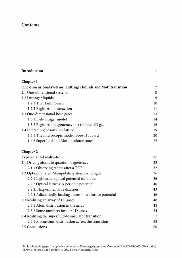
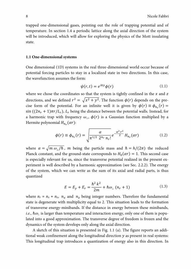
A sketch of this situation is presented in Fig. 1.1 (a). The figure reports an addi-tional weak confinement along the longitudinal direction � as present in real systems: This longitudinal trap introduces a quantization of energy also in this direction. In
Nicole Fabbri8
One-dimensional systems: Luttinger liquids and Mott transition
9
our experiment this longitudinal confinement is indeed well approximated by a har-monic well, so that the term Ey in Eq. (1.3) can be rewritten as Ey � �y (ny + 1/2).
Figure 1.1: (a) Schematics of a system confined to one dimension. Due to the transverse confin-ing potential the transverse degrees of freedom are strongly quantized and only one transverse level is occupied, in contrast to what happens in the axial direction denoted by y: Occupied levels are represented in red; empty levels in gray. (b) Excitation propagating along the 1D system, cor-responding to a density wave with length-scale larger than the interparticle spacing.
If the system is sufficiently anisotropic, i.e., y ≪ , this longitudinal confine-ment does not invalidate the simple picture we have traced up till now, even if it in-troduces some important modification on the system physics, as will be discussed in Sec. 1.3.2. To be precise, if the temperature � and the interaction energy Eint fulfill the condition �y ≤ Eint, T ≪ �, the system still occupies the transverse ground-state, which is degenerate since it includes several longitudinal modes. Commonly in ex-periments atoms do not form a simple chain with thickness of a single atom, but the fulfilling of this condition ensures that the system is one-dimensional.
1.2 Luttinger liquids
Interacting one-dimensional fluids, no matter if the particles are fermions or bosons, belong to a universality class of systems that Haldane [58] termed ‘Luttinger liquids’. The name derives from the analogy with higher dimensional fermionic systems, where the equivalent role is played by the universality class of Fermi liquids. How-ever, unlike the Fermi liquids, the class of Luttinger liquids also includes one-dimensional interacting boson systems. This derives from the absence of a well-defined concept of statistics in 1D. As a consequence, the low-energy degrees of free-dom of the fermions can be described in terms of a bosonic field, and boson systems can display fermion-like properties under certain conditions.
As a general property, because of inter-particle interactions, if any atom tries to move, it inevitably pushes its neighbours along the 1D axis, and the latter their own
9One dimensional systems: Luttinger liquids and Mott transition

Nicole Fabbri
10
neighbours and so on, namely, a density wave propagates along the system. Thus, no individual motion is possible and any individual excitation becomes a collective one. This feature is illustrated in Fig. 1.1 (b). This character also suggests to re-express the excitations in a basis of collective excitations, which is the idea behind the most suc-cessful theory describing 1D systems, the so-called bosonization technique (or har-monic fluid approach), that we will briefly trace in the next section.
1.2.1 The Hamiltonian
In the framework of this theory, the behaviour of interacting particles in 1D is de-scribed by a low-energy effective Hamiltonian which has the form of a harmonic os-cillator [56]
� � ��� ��� �� � �“������ � �
� �“������. (1.4)
Here, “��� and ���� are respectively modulus and phase of the single-particle creation operator � � �“���������; u and K are the so-called Luttinger parame-ter, defined as
� � � ���� , (1.5)
�� � �
��. (1.6)
where � is the mean 1D-density, � the mass of the particles and � the interparticle interaction energy.
These parameters u and K totally characterize any one-dimensional system. For the appropriate K and u, the Hamiltonian in Eq. (1.4) efficiently describes the low-energy properties of the system, no matter what is the microscopic structure of the specific realization. Note that including higher-order terms would not change the form of the Hamiltonian but can be absorbed by renormalizing the parameter K and u, so that H does not depend on the perturbative derivation that makes it a real low-energy effective Hamiltonian.
From Eq. (1.4), one can extract that the excitations are sound-like density waves, with linear dispersion relation ∼ uk where u is the sound velocity. As a conse-quence of the linear spectrum, such a system is a true superfluid [58]. Concerning the dimensionless parameter K, it tends to � � � for noninteracting bosons, and de-creases when repulsive interactions increase. From Eq. (1.5) and (1.6) one can also notice that the ratio between interaction and kinetic energy scales as ��� ∼ ����������. This indicates a fundamental difference of 1D systems with
Nicole Fabbri10
One-dimensional systems: Luttinger liquids and Mott transition
11
respect to their 3D counterpart, i.e., the lower the density the stronger are interac-tions compared to kinetic energy.
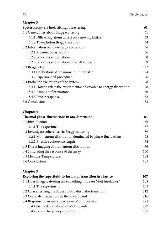
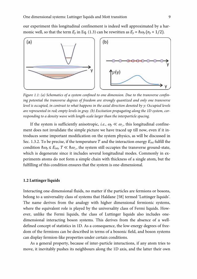
Figure 1.2: Schematic phase diagram for bosononic particles in a 1D system, as a function of the parameter K which describes the strength of interparticle interactions. For K = 0, interactions are so strong to prevent particles to superimpose each others; interactions increase as K decreases, until reaching the limit of no interaction in the limit K .
1.2.2 Regimes of interaction
Interactions imply the presence of spatial correlations between the particles. Thus, key physical properties of interacting 1D systems are defined by means of their corre-lation functions – that are just what we measure in our experiments (see Chapter 3). Remarkably, correlation function in 1D systems show a power-law decay [56] that is universal and only depend on the parameter K. In particular, one can identify the fol-lowing different regimes, reported in the schematic phase-diagram shown in Fig. 1.2.
K = : Non-interacting bosons. As we already noticed from Eq. (1.4) this case corresponds to non-interacting bosons. This is consistent with a superfluid system, where density fluctuations are extinguished. Besides, the single-particle correlation function does not decay with distance, which indicates the system to possess off-diagonal long-range order. In practice, the system is condensed in the zero-momentum state.
1 < K < : Interacting bosons. For finite values of K the one-particle correla tion function has a power-law decay as (2K)‐1. The smaller K, the faster is its decay, and the system manifests weaker tendency to superfluidity.
K = 1: Tonks-Girardeau gas. For point-like interactions, infinite repulsion pre-cisely corresponds to � � 1 [56]. In that case, the density of the system becomes equivalent to that of spinless fermions since the wavefunctions of the particles cannot overlap, but apart from this constrains they are totally free. The density correlation function is that of fermions � � 1����, and 2� is equivalent to 2kF, kF being the Fermi wavevector. This realizes the so-called Tonks-Girardeau gas. Note that the sin-gle-particle correlations do not become equal to that of spinless fermions since statis-
11One dimensional systems: Luttinger liquids and Mott transition
Nicole Fabbri
12
tics are still reflected in it. For pure δ-like interactions, K = 1 is the minimum achiev-able value. Long-range repulsion can induce the system to explore smaller value of K.
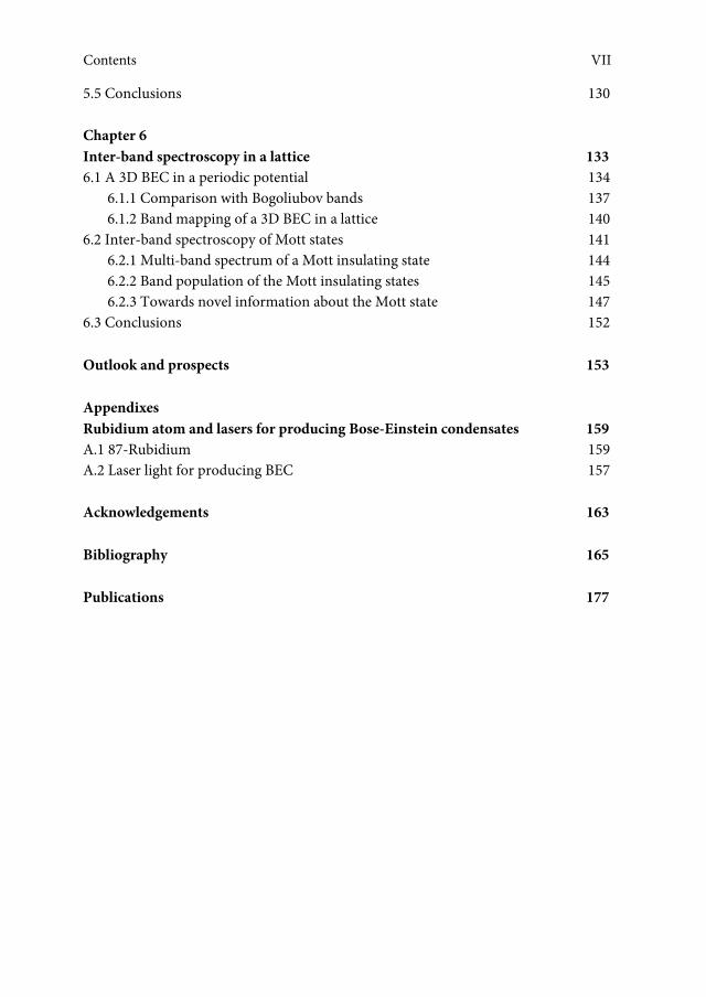
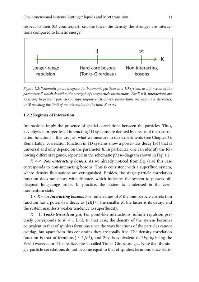
Figure 1.3: The particle-hole excitation spectrum for (a) two- and three-dimensional fermionic system and (b) one-dimensional (bosonic and fermionic) system: The energy of the excitations is reported as a function of its momentum. Below, the schematics of the corresponding excitations are represented.
Now, we present some simple physical arguments that show the peculiar shape of the excitation spectrum of a 1D system, compared to their high-dimensional coun-terpart. A major component of the excitations of strongly interacting bosons or free fermions in one dimension consists in the so-called particle-hole excitations, where a particle is extracted from below the Fermi level (where a hole is created) and pro-moted above it. Since the removed particle has momentum � and the excited one has momentum k’, the momentum of the excitation is well defined, and equal to � � � � ��. Comparing 1D systems of boson or fermion particles with high-dimensional fermionic systems can be insightful. In 2D or 3D for � � �� one can create particle-hole pairs with fixed energy but different momentum. As represented in Fig. 1.3 (a), excitations of arbitrarily low energy can be induced by destroying a particle just below the Fermi energy and creating one just above the Fermi energy, changing the imparted momentum q without moving away from the Fermi surface: This leads to a continuum of energies which starts from zero, for q < kF. In 1D, the Fermi surface is reduced to two points, and since the only way to get a low-energy ex-citation is to destroy and create particles near the Fermi level, the points where the particle-hole excitation energy can reach zero are only � � � and � � ��� .
Nicole Fabbri12

One-dimensional systems: Luttinger liquids and Mott transition
13
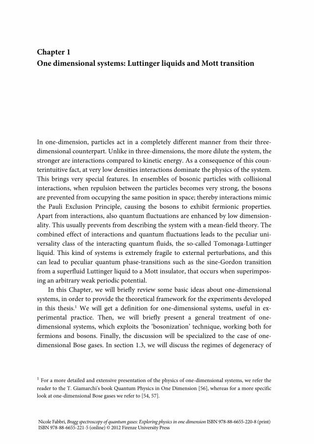
Figure 1.4: Identification of the different branches of the particle-hole excitation spectrum of a one-dimensional system: A particle can be removed from the Fermi surface and promoted to higher-energy, with momentum transfer near to zero or 2�� (blue and purple arrows, respec-tively), otherwise a particle can be extracted well below the Fermi surface, an intermediate value of momentum 0 < q < 2 kF being imparted (red arrow).
The possible excitations in a 1D bosonic gas and the corresponding branches of the excitation spectrum are summarized in Fig. 1.4. As we said before, gapless excita-tions can be induced creating a hole just below the Fermi level and a particle in an energy state above the Fermi level, with momentum � � 0 or � � 2�� as the energy vanishes (blue and purple branches of the spectrum, corresponding to excitations denoted by arrows of the same colour). Besides, for momentum 0 � � � 2�� , the system has gapped excitations (red branch of the spectrum, and corresponding exci-tation, in the figure). The latter consist in creating a hole, well-below the Fermi ‘sur-face’: The removed particle can only jump above the Fermi energy, since all the states below this threshold are already populated and cannot be further occupied because of the Pauli principle for fermions or strong repulsions for bosons; thus a finite jump in energy is necessary.
1.3 One-dimensional Bose gases
In the previous section, we presented a general theory for 1D systems that is valid in-dependently from the microscopic properties of the specific realization. This model provides a general low-energy Hamiltonian, fully determined by two interaction-dependent parameters: the velocity of excitations u and the dimensionless exponent K. The model predicts the elementary excitations of the system and its spatial first-
13One dimensional systems: Luttinger liquids and Mott transition

Nicole Fabbri
14
and second-order correlations functions, the decay of which is universal for all the 1D systems, only depending on the parameter K. Now, we restrict the description to the case of one-dimensional Bose gases, implemented in our experiments.
For describing the properties of a specific realization, it is necessary for connect-ing the Luttinger parameters with known properties of the system considered. Never-theless, for most of the condensed-matter realizations, this is in general a non-straightforward job. Since the details of the interaction are rarely known, only a theo-retical estimate of the power-law exponents is possible, whereas a precise quantitative comparison between theoretical predictions and experiment is usually prevented. The only exception, as far as we know, is recent work on weakly coupled spin-1/2 Heisenberg antiferromagnetic ladders realized by a crystal of CuBr4(C5H12N)2 [60]. Such spin-1/2 ladders in the presence of an external magnetic field map essentially onto a 1D system of interacting spinless fermions. However, suitable spin-ladder sys-tems are rare, either because of unattainable critical fields or because of the presence of anisotropic interactions.
On this prospect, dilute ultracold gases can be a prime candidate to extensively study the Luttinger-liquid physics: They present a major advantage with respect to other realizations of 1D systems, since it is possible to directly connect the micro-scopic properties, such as the particle mass and the density, with the universal Lut-tinger parameters. This allows one to directly compare theory and experiment.
In particular, we will consider bosonic particles that, from the theoretical point of view, show quite interesting peculiarities and are in fact a priori much more difficult to treat than their fermionic counterpart. As a matter of fact, for fermionic systems, the free-fermion model is a good starting point, from which one can gain valuable physical intuition on several problems before adding interactions. On the contrary, for bosons interactions must be taken into account from the beginning, since there are radical differences between a non-interacting boson gas and an interacting one. For instance, superfluidity occurs only in interacting systems: In fact, free bosons at zero temperature have a quadratic dispersion relation, whereas interactions deter-mine a linear dispersion relation at small momenta. The effect of interactions be-comes much more dramatic in one-dimension.
In the following, we will present a model of particles with point-like collisional interactions, suitable for cold bosonic gases as we realize in the experiment.
1.3.1 Lieb-Liniger model
Let us consider an ultracold bosonic gas strongly confined in two directions. Since only very low energies are present, only binary collisions at low energy are relevant: Atoms mainly interact through s-wave scattering, described by the three-dimensional scattering length as. Thus, the details of the molecular potential can be neglected and
Nicole Fabbri14
One-dimensional systems: Luttinger liquids and Mott transition
15
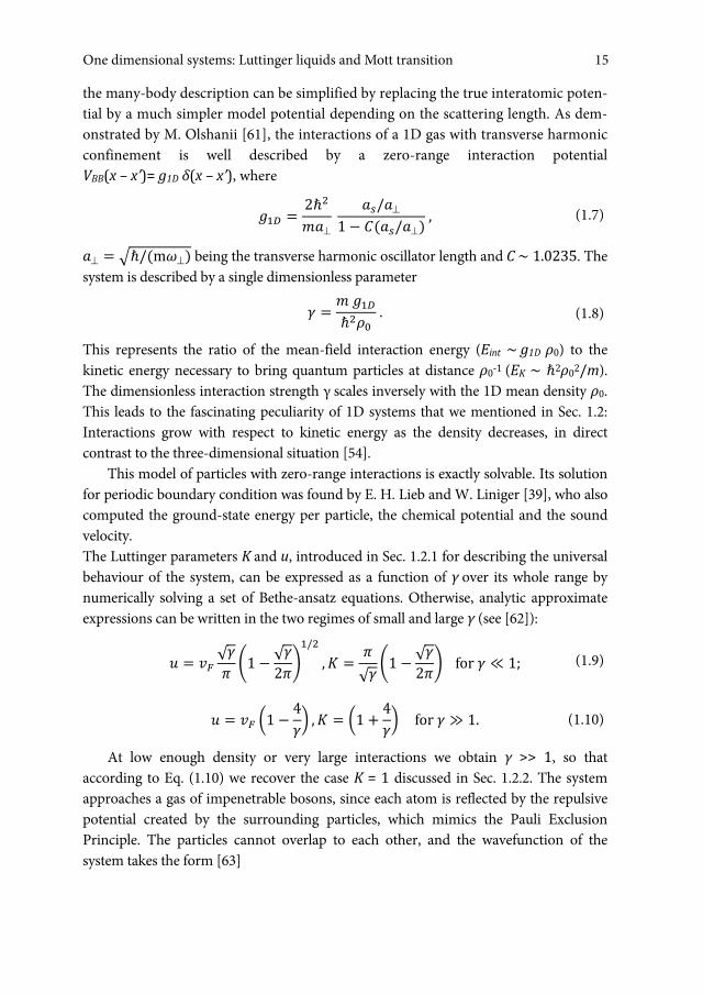
the many-body description can be simplified by replacing the true interatomic poten-tial by a much simpler model potential depending on the scattering length. As dem-onstrated by M. Olshanii [61], the interactions of a 1D gas with transverse harmonic confinement is well described by a zero-range interaction potential VBB(x – x’)= g1D δ(x – x’), where
��� � 2����
��/�1 � ����/�� , (1.7)
� � ��/���� being the transverse harmonic oscillator length and C ∼ 1.0235. The system is described by a single dimensionless parameter
� � � ������� . (1.8)
This represents the ratio of the mean-field interaction energy (Eint ∼ g1D ρ0) to the kinetic energy necessary to bring quantum particles at distance ρ0‐1 (EK ∼ �2ρ02/m). The dimensionless interaction strength γ scales inversely with the 1D mean density ρ0. This leads to the fascinating peculiarity of 1D systems that we mentioned in Sec. 1.2: Interactions grow with respect to kinetic energy as the density decreases, in direct contrast to the three-dimensional situation [54].
This model of particles with zero-range interactions is exactly solvable. Its solution for periodic boundary condition was found by E. H. Lieb and W. Liniger [39], who also computed the ground-state energy per particle, the chemical potential and the sound velocity. The Luttinger parameters K and u, introduced in Sec. 1.2.1 for describing the universal behaviour of the system, can be expressed as a function of γ over its whole range by numerically solving a set of Bethe-ansatz equations. Otherwise, analytic approximate expressions can be written in the two regimes of small and large γ (see [62]):
� � �� √�� �1 � √�2��
�/�, � � �
√� �1 �√�2�� ��� � � 1� (1.9)
� � �� �1 � 4�� , � � �1 � 4
�� ��� � � 1. (1.10)
At low enough density or very large interactions we obtain γ >> 1, so that according to Eq. (1.10) we recover the case K = 1 discussed in Sec. 1.2.2. The system approaches a gas of impenetrable bosons, since each atom is reflected by the repulsive potential created by the surrounding particles, which mimics the Pauli Exclusion Principle. The particles cannot overlap to each other, and the wavefunction of the system takes the form [63]
15One dimensional systems: Luttinger liquids and Mott transition

Nicole Fabbri
16
���, � , �������� ����� � ���� ��
��� (1.11)
which coincides with the absolute value of the wavefunction of a noninteracting gas of spinless fermions.
1.3.2 Regimes of degeneracy in a trapped 1D gas
In cold-atoms experiments realizing 1D systems, an additional trapping potential is always present along the gaseous tubes. The problem of a 1D gas trapped has been treated by D. S. Petrov, G. V. Shlyapnikov and J. T. M. Walraven [54], who identified the different regimes of degeneracy occurring at low temperature. In the following, we will summarize these results and we will define some important quantities that will be useful in the next Chapters.
Our realization, as in other experiments, implies particles to be in a cylindrical trap, tightly confining the gas in the radial direction, with frequency ω greatly exceeding the mean-field interaction (see Sec. 2.3). Then, at sufficiently low temperature the radial motion of particles is essentially frozen as described in Sec. 1.1 and is governed by the ground-state wavefunction of the radial harmonic oscillator. If the radial extension of the wavefunction largely exceeds the characteristic radius of the interatomic potential, the interparticle interaction acquires a 3D character and will be characterized by the 3D scattering length as. In this case, assuming a >> as, Eq. (1.7) simplifies to [61]
��� � 2����. (1.12)
In the presence of a harmonic trapping potential along the axial direction V(y) = mωy2 y2/2, following [54] it is convenient to introduce another quantity to describe the system, in addition to the parameter γ:
� � �������� , (1.13)
which is dimensionless as γ and provides the relation between the interaction strength g1D and the frequency of the axial trap ωy, �� � ��/����� being the amplitude of axial zero-point oscillations. In our experiments, where an array of 1D gases is produced by loading a BEC of 87Rb in a 2D periodic potential, typical numbers are a ∼ 55 nm and ay ∼ 2 μm for the transverse and axial harmonic oscillator lengths, so that α ≈ 6.
Trapped one-dimensional gas can experience three different regimes of degeneracy, provided that T << Td, where Td = N�ωy is the degeneracy temperature [54]. For sufficiently large interparticle interactions and for a number of particles much smaller than a characteristic value N*, at any T << Td a trapped Tonks gas occurs, with a
Nicole Fabbri16
One-dimensional systems: Luttinger liquids and Mott transition
17
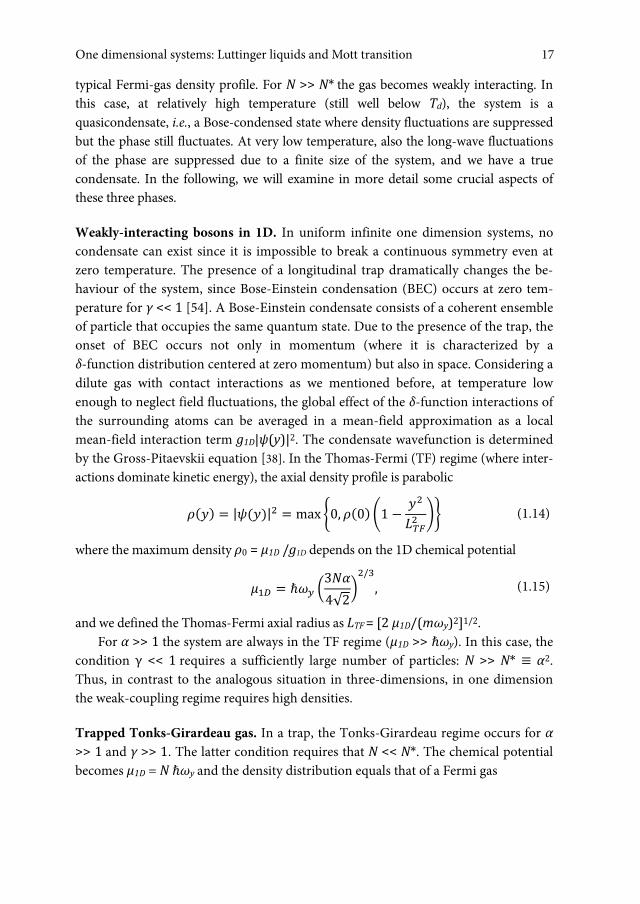
typical Fermi-gas density profile. For N >> N* the gas becomes weakly interacting. In this case, at relatively high temperature (still well below Td), the system is a quasicondensate, i.e., a Bose-condensed state where density fluctuations are suppressed but the phase still fluctuates. At very low temperature, also the long-wave fluctuations of the phase are suppressed due to a finite size of the system, and we have a true condensate. In the following, we will examine in more detail some crucial aspects of these three phases.
Weakly-interacting bosons in 1D. In uniform infinite one dimension systems, no condensate can exist since it is impossible to break a continuous symmetry even at zero temperature. The presence of a longitudinal trap dramatically changes the be-haviour of the system, since Bose-Einstein condensation (BEC) occurs at zero tem-perature for γ << 1 [54]. A Bose-Einstein condensate consists of a coherent ensemble of particle that occupies the same quantum state. Due to the presence of the trap, the onset of BEC occurs not only in momentum (where it is characterized by a δ-function distribution centered at zero momentum) but also in space. Considering a dilute gas with contact interactions as we mentioned before, at temperature low enough to neglect field fluctuations, the global effect of the δ-function interactions of the surrounding atoms can be averaged in a mean-field approximation as a local mean-field interaction term g1D|ψ(y)|2. The condensate wavefunction is determined by the Gross-Pitaevskii equation [38]. In the Thomas-Fermi (TF) regime (where inter-actions dominate kinetic energy), the axial density profile is parabolic
���� � |����|� � ��� �0, ��0� �1 � ������ �� (1.14)
where the maximum density ρ0 = μ1D /g1D depends on the 1D chemical potential
��� � ��� ����4√2��/�, (1.15)
and we defined the Thomas-Fermi axial radius as LTF = [2 μ1D/(mωy)2]1/2. For α >> 1 the system are always in the TF regime (μ1D >> �ωy). In this case, the
condition γ << 1 requires a sufficiently large number of particles: N >> N* ≡ α2. Thus, in contrast to the analogous situation in three-dimensions, in one dimension the weak-coupling regime requires high densities.
Trapped Tonks-Girardeau gas. In a trap, the Tonks-Girardeau regime occurs for α >> 1 and γ >> 1. The latter condition requires that N << N*. The chemical potential becomes μ1D = N �ωy and the density distribution equals that of a Fermi gas
17One dimensional systems: Luttinger liquids and Mott transition

Nicole Fabbri
18
���� � √2���� �1 � ���� (1.16)
where L = (2Nay)1/2 is the axial size of the cloud. As evident from Eq. (1.16), the Tonks-Girardeau profile differs both from the zero-temperature density distribution of a weakly interacting Bose-Einstein condensate and from the spatial distribution of a classical gas.
Finite Temperature: The quasicondensate. Now, let us consider the effect of a finite (even if low) temperature. At finite temperature, longitudinal fluctuations of the den-sity and phase of the condensate are related to elementary excitations of the cloud. The density fluctuations are dominated by excitations with energy of the order of the chemical potential μ1D. Their wavelength is much smaller than the radial size of the condensate. Hence, these fluctuations have the ordinary three-dimensional character, and in one dimension are small. The phase excitations can be divided in two classes: (i) high-energy excitations, with wavelength smaller then the radial size R, having a 3D character; (ii) low-energy axial excitations, with wavelengths larger than R, exhib-iting a pronounced 1D behavior and giving the most important contribution to the long-wave axial fluctuations of the phase. Let us focus on this second kind of phase fluctuations. For a 1D gas trapped along the axial direction, D. S. Petrov, G. V. Shlyapnikov and J. T. M. Walraven [64] also calculated how the mean squared value of phase fluctuations depends on temperature, near the center of the longitudinal trap. Besides, by means of a local density approximation, F. Gerbier et al. [65] have found an approximate analytic expression of the correlation function valid across the whole sample:
⟨����, ����⟩ � |� � ��|������1 � ��/����� . (1.17)
Here L is the total size of the gas, T is the temperature, and we have introduced the coherence length Lϕ (T) = �2ρ/(mkBT), i.e., the mean distance along which the phase of the system varies by 2π, according to [64]. Lϕ essentially depends on temperature and 1D-density n1D. At the center of the trap, �����, ��� varies linearly with the distance, whereas it has some deviation far away from the center. This can be included by redefining the space-dependent coherence �ϕ (y,T) = Lϕ (T)(1 – (y/L)2)2.
In addition to the coherence length, it is also possible to define a characteristic temperature T ϕ [54], related to the former by the relation Tϕ = LϕT/L. At temperatures lower than Tϕ, Lϕ overcomes the total axial size of the atomic cloud and the longitudinal phase fluctuations are negligible. This uniform phase profile, along with the absence of density fluctuations, defines the true condensate. With increasing temperature, phase fluctuations become relevant. However, density fluctuations are still
Nicole Fabbri18

One-dimensional systems: Luttinger liquids and Mott transition
19
negligible up to the degeneracy temperature Td. Thus, in the range Tϕ < T < Td the density profile is still that of a BEC, but phase coherence is lost. The system can be also depicted as a collection of independently fluctuating local condensates and is called a quasicondensate. At temperatures higher than Td, the gas eventually evolves into the classical regime of a Boltzmann gas. Diminishing the number of atoms, Tϕ also decreases: That makes the condition to have a quasicondensate more and more stringent with regard to temperature. Assuming that the condensed fraction largely exceeds the thermal part, which ensures small density fluctuations, the correlation function of the system only depends on the mean square fluctuations of the phase:
⟨����� ����⟩ � ���������� ��⟨���������⟩��. (1.18)
Therefore, the linear dependence of ������ ��� on the axial coordinates (having redefined the space-dependent coherence length in Eq. (1.17) leads to an exponential decay of the first-order coherence function.
1.4 Interacting bosons in a lattice
So far we considered the 1D gases as a continuum of particles. Now we will tackle the problem of an underlying lattice in which the particles move. This is a fundamental problem, since it also describes the situation of electrons in crystalline lattices. One of the most important consequence of the lattice is the possibility for particles (both atoms in an optical lattice or electrons in a crystal) to produce an insulator driven by interactions, known as the Mott insulator.
For describing a one-dimensional system immersed in a periodic potential, two approaches are possible. The first is an extension of the bosonization theory presented in Sec. 1.2.1, and it is especially suitable for systems with large interactions (γ > 1), corresponding to small values of the Luttinger parameter K. For less interacting systems, with γ < 1 (namely, K ≥ 3), a microscopic approach is more often used, such as that provided by the so-called Bose-Hubbard model. In an intermediate regime, the two approaches give the same results.
In the following section we will present the Bose-Hubbard model, which is more suitable for the system we realize in our experiments (0.2 < γ < 0.8). Now instead let us spend some words about the first approach. In the framework of the bosonization theory, a 1D lattice gas is described by the si-ne-Gordon Hamiltonian, given by the sum of the Hamiltonian in Eq. (1.4) and an addi-tional term which describes the periodic potential. The latter term reads:
�� � ��� ��� ����2������ . (1.19)
19One dimensional systems: Luttinger liquids and Mott transition

Nicole Fabbri
20
where VL is the lattice strength and p an integer number. This periodicity leads to a Mott transition for K = 2 [56]. As a matter of fact, the term in Eq. (1.19) becomes relevant for K < 2 and leads to phase ordering in ϕ(y), where density fluctuations are frozen. This realizes a Mott-insulating phase with an integer number of bosons per site. A remarkable fact is that this phase occurs for any amplitude of the periodic potential, even if small.
1.4.1 The microscopic model: Bose-Hubbard
In the cold atoms context, the system is usually described by means of a model which accounts for the microscopic properties of the system. In the regime of deep lattice potential, the atomic wavefunctions in the lattice are strongly localized, and the dy-namics is restricted to a tunnel process between neighbouring lattice sites. Since the typical energy scales involved in the system dynamics are much lower then the energy spacing from the first to the second lattice band, we can consider only the lowest vi-brational state of the system. The system is described in terms of local properties, such as on-site interactions and nearest neighbor tunneling. This is the approach of the Hubbard model [66], introduced to describe electrons in a crystal lattice and valid for any fermionic particles in a strong periodic potential. This model has been ex-tended to bosonic particles, giving the Bose-Hubbard model [67, 68], which employs bosonic operators instead of fermionic It can be obtained starting from a general Hamiltonian of a 3D system in the presence of a periodic potential, expressed in terms of the bosonic field operator ψ(y)
� � ��� ����� �� ��2� �� � ����� � ������������
� �2 ��� ������������������ (1.20)
where g = 4πas�2/m is the 3D interatomic coupling constant. VL is the depth of the lat-tice potential, which we assume to be very strong in the x-z plane in order to create the 1D gases, and weaker along the y (axial) direction. Finally, Vext is an additional slow-varying external potential, always present in cold-atom experiments. The contact interaction between the atoms is expressed by means of a short-range pseudopotential, aS being the s -wave scattering length we already introduced. For a single atom, the eigenstates of such a Hamiltonian are Bloch waves. For a many-body system the wavefunction is described by the sum of an orthogonal and normalized set of wave functions maximally localized on individual lattice sites (Wannier functions):
Nicole Fabbri20
One-dimensional systems: Luttinger liquids and Mott transition
21
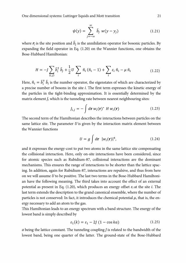
���� � � ����
������� � ��� (1.21)
where rj is the site position and ��� is the annihilation operator for bosonic particles. By expanding the field operator in Eq. (1.20) on the Wannier functions, one obtains the Bose-Hubbard Hamiltonian:
� � ������� ���⟨�,�⟩
� 12� � ���
����� � 1� ���� ���
�� � ��� (1.22)
Here, ��� � ���� ��� is the number operator, the eigenstates of which are characterized by a precise number of bosons in the site i. The first term expresses the kinetic energy of the particles in the tight-binding approximation. It is essentially determined by the matrix element J, which is the tunneling rate between nearest neighbouring sites:
��,� � ���� �����∗ � ����� (1.23)
The second term of the Hamiltonian describes the interactions between particles on the same lattice site. The parameter U is given by the interaction matrix element between the Wannier functions
� � ���� |�����|�, (1.24)
and it expresses the energy-cost to put two atoms in the same lattice site compensating the collisional interaction. Here, only on-site interactions have been considered, since for atomic species such as Rubidium-87, collisional interactions are the dominant mechanisms. This ensures the range of interactions to be shorter than the lattice spac-ing. In addition, again for Rubidium-87, interactions are repulsive, and thus from here on we will assume U to be positive. The last two terms in the Bose-Hubbard Hamiltoni-an have the following meaning. The third takes into account the effect of an external potential as present in Eq. (1.20), which produces an energy offset εi at the site i. The last term extends the description to the grand canonical ensemble, where the number of particles is not conserved: In fact, it introduces the chemical potential μ, that is, the en-ergy necessary to add an atom to the gas. This Hamiltonian leads to an energy spectrum with a band structure. The energy of the lowest band is simply described by
����� � �� � 2� �1 � ��� ��� (1.25)
a being the lattice constant. The tunneling coupling J is related to the bandwidth of the lowest band, being one quarter of the latter. The ground-state of the Bose-Hubbard
21One dimensional systems: Luttinger liquids and Mott transition

Nicole Fabbri
22
Hamiltonian depends on the ratio between the energy scales U and J. First of all, we will consider the two limiting case for a homogeneous system (εi = 0), then we will introduce the effect of an external trapping potential.
1.4.2 Superfluid and Mott insulator states
In the weak interacting case U / J << 1, the tunneling term dominates, and the system is a Bose-Einstein condensate, namely a superfluid state in which the gas can move without friction and particles are delocalized over the whole lattice. The ground-state of the many-body system is given by the superposition of the Wannier wavefunctions with the same phase. For N particles on M lattice sites, this can be written as
|Ψ��⟩���� ∝1√�������
�
�����|0⟩ (1.26)
Since the many-body state is the product of identical single-particle states, it can be described by a single macroscopic wavefunction |ϕi, which is equivalent to a coherent state. Thus, the expectation value of the field operator ϕi|��� |ϕi is nonzero. The number of atoms on each lattice site is affected by the maximum uncertainty. In the limit of a large system size M, N with constant average occupation n = N/M; this state becomes separable into a product of single-site states, which are the superposition of Fock states |�� � ������|0⟩ for all possible n. The number of atoms on each site follows a Poissonian statistics, the variance of which is given by the average occupation. Increasing the interaction strength U, the properties of the system change drastically. Let us consider now the limiting case U/J >> 1, where the system experiences an inter-action-induced insulating phase, the so-called Mott insulator. The atom number fluc-tuations due to the delocalization of the wavefunction are unfavourable, as configura-tions with more than one atom per site have an energy cost. The many-body ground state consists of localized wavefunctions, which minimize the repulsive interaction. The global wavefunction can be expressed as a product of local Fock states, which are the eigenstates of the number operator on each lattice site. Supposing we have a configura-tion with one atom per site (which is reasonable in the homogeneous case), we obtain
|Ψ��⟩��� ∝��������
�
���|0⟩ (1.27)
The number of atoms per site is defined, and the mean value of the field operator vanishes. Thus, the conjugate variable of the atom number, that is the phase, has the maximum uncertainty. This is in strong contrast to the superfluid case, where the phase is well-defined throughout the whole ensemble.
Nicole Fabbri22

One-dimensional systems: Luttinger liquids and Mott transition
23
Quantum phase transition. When the strength of the interaction term relative to the tunneling term is changed, the system reaches a quantum critical point in the ratio of U/J, where it undergoes a quantum phase transition from the superfluid to the Mott insulator ground-state. This transition is induced by quantum fluctuations, whereby it occurs also at zero temperature, where thermal fluctuations are suppressed [69]. In the context of cold atoms, the parameters U and J can be arbitrarily tuned by varying the experimental parameters, as will be illustrated in the next Chapter. This offers the un-precedented possibility to monitor such a transition. For three-dimensional systems, the quantum critical point (U/J)c can be calculated using the mean-field approach [67, 70, 71, 72], giving an accurate estimate of it, in agreement with more sophisticated cal-culations [73]: (U/J)c ≃ 5.8 × z (z being the number of nearest neighbours) for n ≤ 1 and (U/J)c ≃ 4 × z n for n >> 1. In one dimension, relevant deviations are observed from the mean-field prediction. In this case, the transition takes place at (U/J)c = 3.84 for unity occupation and (U/J)c = 2.2 n for n >> 1 [74, 75].
Phase diagram of a trapped gas. In cold-atom experiments, an external trapping po-tential is always present. It can be produced by an inhomogeneous magnetic field or by the spatial profile of red-detuned gaussian beams which create the optical lattice potentials (see Sec. 2.2.2). Now, we consider only its contribution along the axial di-rection, assuming it to be negligible in the transverse plane with respect to the trap-ping frequencies in the lattice sites.
In the Bose-Hubbard Hamiltonian, this is taken into account by the term ��� ��� that we mentioned before. Typically, the energy offset εi varies slowly compared to the typical size of the atomic cloud, and the external potential experienced by the at-oms is well approximated by a harmonic term εi = (m ωy2y2)/2.
In the superfluid regime, the trap effect can be introduced in the mean-field picture by means of a local density approximation (LDA). Namely, we assume that the system behaves as in the homogeneous case, with a spatially-varying chemical potential μ(y) = μ(0) – ε(y), where ε(0) = 0 at the center of the trap.
This produces a slow modulation of the density, which is maximum at the trap center and decays to zero at the edge. The average occupation number in the site i can be determined by minimizing the local potential energy, given the chemical po-tential of the system:
�� � ��� �0, � � ��� � (1.28)
which yields the Thomas-Fermi distribution described in Eq. (1.14), where the Thomas-Fermi radius is determined by imposing the potential energy to be equal to the global chemical potential. This overall density modulation constitutes the envelope of the single-site Wannier functions.
23One dimensional systems: Luttinger liquids and Mott transition

Nicole Fabbri
24
Figure 1.5: (a) State diagram of a homogeneous one-dimensional Bose gas in the presence of a lattice potential. The presence of an additional slow-varying trap can be described in terms of a spatially-dependent chemical potential (green dashed line). The figure is adapted from [71]. (b) State diagram for a one-dimensional Bose gas in a lattice with a harmonic confining potential. The state diagram was built using a trap with mωy2/J = 0.008 in which the gas has total size L = 100 sites. On the vertical axis, the characteristic density ρc of the gas is reported (see text). The figure is adapted from [76].
The LDA gives a useful, even if approximate, insight of the effect of the confinement. According to the LDA, a single experimental realization is not represented by an isolated point in the phase-space J/U – μ/U, but rather by a line which extends over several values of μ, as represented in Fig. 1.5 (a). This line intersects both the superfluid region and different Mott-insulating lobes, corresponding to different average occupation of the lattice sites.
The state diagram of a one-dimensional Bose gas in a trap has been recently computed by M. Rigol et al. in [76] via Monte-Carlo calculations. The state digram is defined in terms of a scaled dimensionless variable, the characteristic density
�� � ������� (1.29)
where a is the lattice spacing and N the number of atoms in the gas. ρc is a dimensionless quantity, being (mωy2/J)‐1/2 a length. Essentially, for trapped systems ρc is the analog of the filling per site n = Na/L in the homogeneous case (L being the total length of the tube). Introducing this scaled density has an advantage: It allows the building of a state-diagram in the plane ρc – U/J that is insensitive to the number of atoms and the trap curvature mωy (see Fig. 1.5 (b)). Region (I) represents a pure superfluid phase, (II) a Mott insulating phase at the center of the trap surrounded by a superfluid phase with
Nicole Fabbri24

One-dimensional systems: Luttinger liquids and Mott transition
25
n < 1 , (III) a superfluid phase with n > 1 at the center of the trap surrounded by a Mott insulating phase with n = 1, and an outermost superfluid phase with n = 1.
Figure 1.6: Density profile in one-dimensional trapped systems for different values of the ratio U/J. Different colours represent different temperatures, as labeled in (a). The black straight line describes the profile of the homogeneous system with average occupation n = 1 [76].
Thus, the Mott insulating regions exist above a threshold value of the interaction strength, even without the commensurate filling required in the non-confined case, and they coexist with superfluid domains. This is a practical advantage for experimentalists, since in inhomogeneous systems Mott insulating domains appear for a broad range of fillings, compared to the few commensurate fillings required for the translationally invariant system. This is a unique feature which distinguishes the behavior of a confined system. Figure 1.6 shows the expected density profile of an inhomogeneous Mott insulating state calculated in [76], for different ratios of interaction strength to the tunneling energy (U/J = 10, 14, 16): For U/J = 10 and U/J = 14 the smooth profile of a superfluid can be recognized on top of the Mott insulator plateau.
25One dimensional systems: Luttinger liquids and Mott transition


Chapter 2 Experimental realization
For the projects presented in this thesis, atomic vapours of Rubidium-87 driven to the quantum degenerate phase of a Bose-Einstein condensate are used as a source of ultracold atoms. This three-dimensional gas is confined in an array of one-dimensional microtubes, which constitute our test-ground to investigate the Luttinger physics, covering also the Bose-Hubbard model when the one-dimensional systems are immersed in a periodic lattice along their axis. Typically, the experiments consist of several steps, globally lasting approximately two minutes, to prepare the quantum gas, load it into an optical potential, conduct the actual experiment and then measure the result. These stages are performed in cycles, since the measurements include the observation of the atomic cloud by absorption imaging, which is a destructive technique, since it induces a major heating of the sample and destroys the condensate. This Chapter is intended, on the one hand, to describe how in practice, starting from atomic vapours, ultra-cold one-dimensional gases are prepared in a superfluid or insulator state, illustrating the experimental apparatus and procedure. On the other hand, we will trace a model for inferring the specific features of these gases that determine their physical behavior.1F1F1F
2 How the investigation of these systems has been managed, including the new setup planned and built for spectroscopic measurements, will be instead the object of the next Chapter.
Let us mention that the setup aimed at producing a Bose-Einstein condensate of Rubidium-87 (87Rb) was originally developed at LENS, where it has been working since 1999. Its basic parts have been already described in several publications and theses [77, 78, 79, 80, 81, 82, 83, and 84]. Therefore, in the following only a brief introduction of the operating principle and of the key properties of this experimental setup will be given. The description will be detailed only in those aspects with special relevance for the experiments discussed in the later Chapters, such as the imaging procedure of the atomic cloud.
2 For instance, density influences strongly the ratio of interactions to kinetic energy of the particles.
Nicole Fabbri, Bragg spectroscopy of quantum gases: Exploring physics in one dimension isBN 978-88-6655-220-8 (print) isBN 978-88-6655-221-5 (online) © 2012 Firenze University Press
Nicole Fabbri
28
Most of the attention will be payed to the realization of periodic optical potentials by means of coherent-light standing-waves, based on atom-light dipole interaction. These potentials have played a major role in this thesis, having been exploited to arbitrarily change the geometry of the system, namely to trap the atoms in an array of one-dimensional micro-tubes. The modeling of the global system is complicated by the non-uniform density distribution over the array. In order to describe such a complex situation, we develop a model which extends the calculations presented in the theoretical work in Ref. [55] and allows us to entirely characterize each tube of the array. An optical lattice added along the axis of the tubes has also been used to directly tune the ratio between the atom-atom interactions and the tunneling along the periodic potential, in order to realize an atomic Mott insulator.
2.1 Driving atoms to quantum degeneracy
In the following, we will explain the experimental procedure used to obtain a 87Rb Bose-Einstein condensate in the low-field-seeking state |F = 1, mF = – 1 that can be trapped in a magnetic field minimum. For the scheme of the energy-level structure of 87Rb, see Appendix A.1.
As a first step, a double-stage magneto-optical trap (MOT) is used to collect atoms from a room temperature gas within ∼ 90 s. This trap also cools the atoms, especially in the last phase which employs optical molasses. In a second step, the atoms are transferred in a pure magnetic quadrupole trap. Finally, the latter is modified into a quadrupole-Ioffe configuration (QUIC), and the cloud is cooled further for up to 60 s via forced evaporation until a BEC is formed.
Double-stage Magnetic Optical Trap (MOT). The basic idea of a MOT is to exploit dissipative light forces which introduce an effective friction force to slow down and cool an atomic gas [85]. At the same time, an inhomogeneous magnetic field with a minimum at the center of the trap is applied: It introduces a spatial dependence of the light-force in the form of a linear-elastic force pushing atoms toward the center, leading to a confinement of the atom cloud [86]. The schem-atic setup for a MOT is shown in Fig. 2.1 (a).
In our experiment, two consecutive MOTs have been implemented. They exploit the D2 transition connecting the fine-structure states 52S1/2 and 52P3/2 at a wavelength λ = 780.246 nm. The cooling laser beams are resonant with the hyperfine transition |F = 2 |F’ = 3, which is the strongest closed one of the hyperfine structure. A strong loss channel is constituted by atoms which populate the state |F’ = 2 – a process made possible by the fact that the hyperfine splitting of the two excited state is quite narrow (∼ 266.6 MHz) – and may decay from this state into the uncoupled |F = 1 state (the
Nicole Fabbri28
Exploring the superfluid-to-insulator transition in a lattice
29
hyperfine ground-state splitting is 6.8 GHz, so that the cooling light is completely off-resonance with respect to it). For this reason, we apply a repumper laser on the |F = 1 |F’ = 2 transition to return the atoms that have fallen into the |F = 1 ground-state back to the cooling transition.
The first MOT is produced in a first stainless steel chamber, connected to a cell which hosts a rubidium sample: The flux of vapour to the main chamber is regulated through a valve. A moderate ultra-high-vacuum environment is kept, with measured pressure of the order of 10‐9 mbar, for guaranteeing thermal isolation of the sample from the environment. The laser beams we use are red-detuned with respect to the frequency of the cooling transition by 12 MHz ≃ 2 ΓD2, where ΓD2 is the line-width of the D2 transition. The beams have a large diameter (30 mm) to capture a large number of atoms from the background gas. A magnetic field gradient of 7 Gauss/cm is produced by two coils in anti-Helmoltz configuration with a current of 4 A. Typically, ∼1010 atoms are caught at a temperature of ∼ 100 μK, with a loading time of ∼ 5 s. Then, the atoms are transferred to a second vacuum cell, where a second MOT stage is implemented, followed by the other steps leading to condensation. The transfer to the second chamber is carried out by a pulsed push beam with σ+ circular polarization and red-detuned by 3 MHz relative to the cooling transition, through a thin steel pipe2F2F2F
3 which maintains a differential vacuum between the two MOT cells. The pressure of the second cell is of the order of 10‐11 mbar, required for the good operation of the magnetostatic trap which is created in the same cell. Therefore, the second MOT does not capture atoms from background gas, but only those precooled by the first MOT and transferred to the second one. The cooling light for the second MOT is red-detuned again by 2 ΓD2 from the resonance and the beams have a diameter of 20 mm. The quadrupole field is generated again by a pair of anti-Helmoltz coils, producing a magnetic field gradient of 10 Gauss/cm. Three pairs of Helmoltz coils are used to cancel spurious magnetic fields. About 1010 atoms are captured and brought to a temperature3F3F3Fof ∼ 100 μK. 4
Compressed-MOT and Molasses. Before transferring the atoms in the magnetic trap, the atomic density must be increased. To this purpose, at the end of the MOT
3 The transfer is optimized thanks to a series of permanent magnets surrounding the tube, which create an hexapolar magnetic field with a local minimum at the center of the tube and thus focus the beam of atoms optically pumped into the Zeeman state |F = 2, mF = 2. 4 Note that laser cooling suffers from an intrinsic limitation: The lowest achievable temperature is the recoil temperature Tr = �2k2/(mkB), where k = 2 π/λ is the wave-number of the cooling radiation and m is the mass of 87Rb. This corresponds to the kinetic energy acquired in a photon-absorption process. For Rubidium, it is ∼360 nK.
29Experimental realization

Nicole Fabbri
30
phase, a compression of the atomic cloud is performed for 20 ms by modifying the magnetic-field gradient from 10 G/cm to 6 G/cm and increasing the detuning of the cooling beam from 12 MHz to 24 MHz [87, 88]. This allows the density to grow by one order of magnitude, but the temperature is still too high for an effective transfer to the magnetic trap. Then, we further cool the atoms in a 5 ms-long optical molasses [89]. In the molasses phase, the magnetic field is turned off and the detuning of the cooling beams is increased to 48 MHz, whereas their power is reduced by a factor 2. In conclusion, after the com-pressed-MOT and molasses phases, the gas has tem-perature of ∼ 50 μK and density n ∼ 1010 cm-3, driving the sample to a phase-space density of 10‐7. In Appendix A.2, a scheme summarizes the laser frequencies used for our experiment.
Figure 2.1: Key-mechanisms for driving atoms to quantum degeneracy. (a) Schematic of a mag-neto-optical trap: Atoms are trapped in the intersection region of three pairs of counterpropagating red-detuned lasers beams with opposite circular polarization (orange ar-rows), thanks to the combined effect of friction and elastic forces exerted in the presence of a quadrupole magnetic field, the flux lines of which are represented by gray arrows). (b) Principle of radiofrequency-forced evaporative cooling. A radiofrequency field is used to induce ener-gy-selective transitions to an untrapped Zeeman sublevel. Most energetic atoms are removed from the trap, whereby the system can thermalize at a lower temperature.
Optical pumping. At this point, atoms are transferred to the low-field-seeking state |F = 1, mF = – 1 by means of a two-step optically-pumping process. By turning off the cooling light ∼ 200 μs before the repumping light used for the molasses, atoms are forced to decay to the hyperfine sublevel |F = 2 of the ground-state. Then, we ap-ply a weak magnetic field which defines a quantization axis for the atoms and, simul-
Nicole Fabbri30

Exploring the superfluid-to-insulator transition in a lattice
31
taneously, a light-pulse resonant with the transition |F = 2 |F’ = 2 traveling in the same direction as the field and circularly polarized: In this way, the |F = 2 state is completely emptied and atoms end up to decaying to |F = 1, with a bias towards the Zeeman state |mF = –1.
Magnetic trapping. The atoms in |F = 1, mF = – 1 are then loaded in a conservative potential, constituted by a pure magnetic trap, where further cooling can be imple-mented. As a first stage, we turn on a pure quadrupole field with a gradient higher than the one used for the MOT, appropriately chosen to recapture as many atoms as possible in the trap (70 G/cm along the vertical direction and 35 G/cm in the radial plane, produced by a current of 70 A). Then, we further enhance the gradient, by in-creasing the current in the quadrupole coil up to 235 A, in order to improve the phase-space density of the atomic cloud in the trap [78]. Nevertheless, the quadrupole field is unsuitable to obtain Bose-Einstein condensation, since it vanishes at the center of the trap, and its direction changes rapidly around this point. For at-oms passing at a close distance from the trap center, the Larmor precession frequency is low enough that their spin cannot adiabatically follow the rapidly changing field direction. Thus, atoms may undergo spin-flips to untrapped states [90], leading to atom losses, which become significant as the temperature drops when approaching quantum degeneracy [91, 17]. The solution adopted in our experiment is a static field which varies harmonically around a nonzero local minimum, as in the Ioffe-Pritchard configuration [92, 93]. This is obtained by using an additional coil oriented perpendicularly to the quadrupole pair, which produces a field-curvature. In this configuration, the atoms in the hyperfine state |F = 1, mF = – 1 experience a trap with cylindric symmetry with measured frequencies ωy = 2 π × 8.8 Hz and ω = 2 π × 87 Hz, and an offset field B0 ≃ 2.5 G. Evaporative cooling. In the magnetic trap, the temperature of the cloud is further reduced by energy-selective radiofrequency (RF) evaporation (see e.g. [94, 95]) In the presence of the inhomogeneous magnetic field the atomic Zeeman-shift is posi-tion-dependent. Therefore an RF-field with narrow linewidth can excite the transi-tion from the initial trapped state |F = 1, mF = – 1 to the untrapped state |F = 1, mF = 1 only in a given region of the trap, where the energy of the RF photon matches the Zeeman shift between the levels. The transition-frequency at the poten-tial minimum is typically 2 MHz for the trap described above. Using higher frequen-cy, atoms at certain distances from the trap center are in resonance with the radiation and thus fall into the untrapped state. After selectively removing the outermost atoms of the cloud, which have the highest energy, the average energy of the sample reduces and the cloud equilibrates at a lower temperature via elastic collisions. An RF-sweep of about 60 s, with shrinking frequency, allows for the covering of several orders of
31Experimental realization
Nicole Fabbri
32
magnitude in temperature until quantum degeneracy is reached at a critical tempera-ture of approximately 125 nK and a Bose-Einstein condensate is formed with about 4 × 10⁵ atoms.
2.1.1 Observing atoms after a TOF
Resonant light absorption can be employed to image the atomic cloud. Essentially, a beam of resonant light is directed onto the atoms and then is detected by a CCD camera, which records the shadow cast by the atoms on the spatial beam profile. In cold atom experiments, this is the most common way to extract some basic data about the system. In the work of this thesis, we widely exploit resonant absorption imaging to get complementary information to that obtained from Bragg spectroscopy, such as to measure the momentum distribution of the atoms.
For our experiments, a precise knowledge of the global number of atoms of the atomic cloud is a fundamental requirement to characterize the array of 1D gases we produce. In particular, it is necessary to evaluate the 1D density of each gas, according to the theoretical model we will develop in Sec. 2.3, which is a critical parameter on which the physical behaviour of the system depends. For this reason, we decided to perform a new calibration of the imaging technique following the procedure proposed in [96].
Absorption imaging method. For the imaging conducted in this experiment, we use a 150 μs-long light pulse resonant with the closed hyperfine transition |F = 2 |F’ = 3. Since the Bose-Einstein condensate is produced in the state |F = 1, mF = – 1, a pumping pre-stage into the hyperfine sublevel |F = 2 of the ground-state is performed, inducing atoms to perform a transition |F = 1 |F’ = 2 from which they may decay through the two relaxation channels |F’ = 2 |F = 1 and |F’ = 2 |F = 3. After a few pumping optical cycles, it emp-ties the sublevel |F = 1. The pumping light pulse is ∼ 100 μs-long, chosen to maxi-mize the number of atoms later revealed by the probe light. The probe beam is colli-mated with a diameter much larger than the atomic cloud size, and travels along the direction x of our coordinate system.5 While passing through the cloud, the beam is attenuated due to the absorption by the atoms,6 which at a given position is propor-tional to the 3D density of the atoms.
5 We anticipate here that it is transverse to the direction of the 1D gaseous microtubes we produce. 6 Concerning the internal state of the atoms, after a short transient, the atomic population starts to cycle between the levels |F = 2 and |F = 3.
Nicole Fabbri32

Exploring the superfluid-to-insulator transition in a lattice
33
The light absorption is described by the Beer-Lambert law. Considering possible saturation effects of the resonant incident light, we can write
���� � �� �� ����
1 � ����/����� (2.1)
where dI is the attenuation of the intensity I in a distance dx, n is the numerical 3D den-sity and σ0 = 3 λ2/2π is the resonant absorption cross-section for a two-level atom, λ being the wavelength of the incident light. I0sat = �ω3 ΓD2/(12 πc2) is the saturation intensity for the corresponding two-level transition, c being the speed of light and ω = 2 πc/λ. In the specific case of 87Rb, we have I0sat ∼1.67 mW/cm2 [97]. Note that here we considered the simple case of an atomic ensemble of 87Rb uniformly populating the sublevels of the five-fold |F = 2 ground-state, which is excited by circularly polar-ized light propagating along the quantization axis of the atoms at the D2 line.
In a more general case, the response of the atoms, i.e., the population driven into the excited state by the imaging laser beam is affected by a non-perfectly circular polar-ization of the imaging beam, the manifold structure of the excited state, and the differ-ent Zeeman sublevel populations of the degenerate ground state of the optical transi-tion. This can be taken into account by defining an effective saturation intensity Ieffsat = α* I0sat, where the dimensionless parameter α* accounts for the mentioned cor-rections. With the appropriate substitutions, the Beer-Lambert law can be written in the same form as before [96]:
���� � �������
����1 � ����/������� (2.2)
����� � ��/α∗ is the effective cross section including saturation correction. Integrating over the optical path, one can obtain the optical depth
�����, �� � ��� ���, �, � � ���, �; �∗� (2.3)
where f(y,z;α*) is defined by
���, �; �∗� � ��∗ �� �����, ������, ��� �����, �� � ����, ��
����� (2.4)
In practice, to extract Ii(y,z) and If(y,z), we acquire four images which capture re-spectively the probe beam profile with and without the atoms (Iw and Iwo), and the background light in the absence of the probe beam (Idark, 1, Idark, 2 ). These images are processed in order to obtain the intensity before and after the cell, removing the background
����, �� � �����, �� � �����,���, �� (2.5)
33Experimental realization
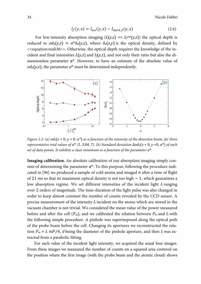
Nicole Fabbri
34
����, �� � �����, �� � �����,���, �� (2.6)
For low-intensity absorption imaging (Ii(y,z) << I0sat(y,z)) the optical depth is reduced to od0(y,z) ≃ α*δ0(y,z), where δ0(x,y) is the optical density, defined by <<equation:reali36>>. Otherwise, the optical depth requires the knowledge of the in-cident and final intensities Ii(y,z) and If(y,z), and not only their ratio but also the di-mensionless parameter α*. However, to have an estimate of the absolute value of od0(y,z), the parameter α* must be determined independently.
Figure 2.2: (a) od0(x = 0, y = 0, α*) as a function of the intensity of the detection beam, for three representative trial values of α* (1, 3.84, 7). (b) Standard deviation Δod0(x = 0, y =0, α*) of each set of data points. It exhibits a clear minimum as a function of the parameter α*.
Imaging calibration. An absolute calibration of our absorption imaging simply con-sists of determining the parameter α*. To this purpose, following the procedure indi-cated in [96] we produced a sample of cold atoms and imaged it after a time of flight of 21 ms so that its maximum optical density is not too high ∼ 1, which guarantees a low absorption regime. We set different intensities of the incident light Ii ranging over 2 orders of magnitude. The time-duration of the light pulse was also changed in order to keep almost constant the number of counts revealed by the CCD sensor. A precise measurement of the intensity Ii incident on the atoms which are stored in the vacuum chamber is not trivial. We considered the mean value of the power measured before and after the cell (Pm), and we calibrated the relation between Pm and Ii with the following simple procedure. A pinhole was superimposed along the optical path of the probe beam before the cell. Changing its apertures we reconstructed the rela-tion Pm = Ii πd2/4, d being the diameter of the pinhole aperture, and then Ii was ex-tracted from a parabolic fitting.
For each value of the incident light intensity, we acquired the usual four images. From these images we measured the number of counts on a squared area centered on the position where the first image (with the probe beam and the atomic cloud) shows
Nicole Fabbri34
Exploring the superfluid-to-insulator transition in a lattice
35
the peak density, and with extended over few pixels (the side being ∼ 0.1 of the half width at half maximum of the peak profile). This defines in practice Iw, Iwo, Idark,1, Idark,2 from which we extract the optical depth od0(0, 0) using Eq. (2.3) for different trial values of α*. Figure 2.2 (a) reports the results of such measurements of od0(y,z) for α* = 1, 3.8, 7.
Since the optical depth must depend only on the cloud properties, the appropriate value of α* is the one that has a minimum dependence on the incoming intensity. In practice, we infer by a least-squares method our best estimate of α* for which od0(α*) has a minimum standard deviation over the whole range of incident intensities used to image the cloud, as shown in Fig. 2.2 (b). We find α* = (3.84 ± 0.04). Scaling laws. The optical resolution of our imaging apparatus is comparable with the global size of the atomic cloud along its more confined direction.7 Thus, the observa-tion of the atomic cloud is performed after turning off the trapping potential and let-ting atoms to ballistically fall for a certain time-of-flight.
In our experiment, the atomic cloud is confined in a highly elongated trap. This is already true for the 3D BEC in the magnetic trap, and becomes much more pronounced for the 1D gases we produce in the optical lattices we will present in the next Section. As a consequence of the Heisenberg uncertainty principle (ΔpΔx � �) which the system follows due to its quantum nature, the atomic ensemble undergo as a strongly anisotropic expansion, which is faster in the direction where the confinement was stronger. The temporal evolution of a BEC in the Thomas-Fermi regime in the presence of an external time-dependent potential is well-known. This is described in the theoretical works by Y. Kagan, E.L. Surkov and G.V. Shlyapnikov [98] and Y. Castin and R. Dum [99]. The evolution of the spatial density is essentially a dilatation, which does not mod-ify the form of its spatial dependence but implies a rescaling characterized by three scal-ing factors which allow a classical interpretation of the dynamics. This analytic treat-ment can be easily adapted to the evolution of a BEC released from a cigar-shaped trap (see [100]). For a cigar-shape condensate, as we produce, the half-lengths of the con-densate evolve during expansion according to the following equations
���� � ��0��1 � �� (2.7)
���� � ��� ��0� �1 � �� �� ������ � �1 � ���� (2.8)
7 The limiting factors of our imaging system are the finite numerical aperture of the optics along the probe beam path and the optical quality of the cell windows, which sets a resolution limit to ∼ 8 μm.
35Experimental realization
Nicole Fabbri
36
where τ = ωt and ϵ is the aspect ratio of the trap (ϵ = ωy/ω). Time-of-flight absorption imaging will be retrieved later on, particularly in Sec.
2.4.1 where we will discuss the feature of an atomic cloud released from an optical lattice potential. Besides, in Chapter 4 we will present an experiment demonstrating that time-of-flight measurement can be used to probe the coherence length of an array of one-dimensional gases.
2.2 Optical lattices: Manipulating atoms with light
Laser light can be exploited to trap neutral atoms in attractive or repulsive conservative potentials, the shape and depth of which can be easily engineered and dynamically controlled. Attainable trap depths in a tightly focused beam are typically in the millikelvin range, orders of magnitude smaller than the thermal energy of atoms at room temperature. Once a gas has been driven to the ultralow temperatures necessary to reach Bose-Einstein condensation at moderate density, it can be easily trapped in these weak potentials.
This section will present some general aspects of the optical potentials, particularly focusing on their periodic version (optical lattices) where atoms are axially confined in the nodes or antinodes of a standing wave. We will introduce some useful notations and we will describe the experimental setup.
2.2.1 Light as an optical potential for atoms
Now, we would like to recall the key principles which allow us to exploit laser light to realize an optical potential for atoms.
The electromagnetic interaction of atoms with laser light consists in a coupling between the electric dipole of the atoms and the electric field of the light. As is well-known, an atom undergoes two different forces, respectively associated with the dissipative and the dispersive properties of the interaction.
The dissipative force, also called the radiation pressure force, is proportional to the gradient of the field phase, and is responsible for the momentum-transfer from light to atoms in a resonant scattering process. As such, it is at the origin of the development of laser cooling of atoms, which has been described in Sec. 2.1. Here instead we will deal with the dispersive part of the atom-light interaction, which determines the dipole force. This force is proportional to the intensity gradient of the field. Because of its conservative character, it can be derived from a potential, the minima of which can be used for atom trapping in different geometries. For a complete theoretical analysis of these effects, we refer to [85]. The results presented in the following can be simply obtained using a textbook semiclassical approach [101], by considering the atom as a
Nicole Fabbri36

Exploring the superfluid-to-insulator transition in a lattice
37
two-level quantum system interacting with a classical radiation field. This will enable us to draw out some useful expression for the reactive and dissipative component of the radiation force, in a simple way.
When an atom is illuminated by laser light, the electric field E(r,t) induces an atomic dipole moment d(r,t) that oscillates at the driving frequency of the field ωL/(2π). In the complex notation E(r,t) = ê E(r)exp(–iωLt) + h.c. and d(r,t) = ê |d(r)| exp(–iωLt) + h.c., where ê is the unit polarization vector. We define the atom polarizability αP describing the relation between the amplitude d of the dipole moment and the field amplitude E as
|�| � ��|�| (2.9)
where αP strongly depends on ωL. This relation holds only in the linear regime, when saturation effects can be neglected and the atomic population is almost entirely in the ground state. While the imaginary part, describing the out-of-phase component of d, is connected with the absorptive properties, the real part of αP describes the component of d oscillating in phase with E and is responsible for the dispersive properties of the interaction, in which we are mainly interested now.
Dipole potential. The interaction potential of the induced dipole moment d in the driving field E is given by
������� � �12 ⟨� � �⟩ � � 12��� Re������������. (2.10)
I(r) = 2ϵ0c|E|2 is the field intensity, ϵ0 being the vacuum dielectric constant. The factor 1/2 takes into account that the dipole moment is an induced, not a permanent one. Note that Udip(r) is a time-independent quantity. As a matter of fact, the motion of the center of mass occurs in a time-scale t much bigger than the inverse of ωL: t � �/ER where ER is the recoil energy acquired by an atom having absorbed a photon, given by ER = �2 kL2/(2m). Thus, we consider the average over the rapidly-oscillating field terms, indicated by the angle brackets . The physical origin of such an optical potential which atoms experience is the so-called dipole force [101] obtained by differentiating Eq. (2.10):
������� � � �������� � 12��� Re�������� �����. (2.11)
This force is proportional to the intensity gradient LI(r), so it vanishes when the field intensity is uniform, as in a plane wave. Vice versa, an inhomogeneous intensity field can be exploited for producing potential wells whose features can be changed by tuning the laser parameters.
37Experimental realization

Nicole Fabbri
38
A semiclassical approach [101] is suitable to derive an analytic expression for the atomic polarizability αP and Udip(r), by assuming that the laser light is far-detuned compared to the atomi transition frequency, with very low saturation effects and very low scattering rates, as in common cold atoms experiments. Thus,
������� � 3���
2�� �Γ
�� � ��� �� � ��
� ����
� 3���2�� �Γ∆� ����.
(2.12)
On the right hand side of this expression, we have employed the rotating wave approximation (RWA), which can be used as long as the laser is tuned relatively close to the resonance at ω0 such that the detuning Δ = ω0–ωL fulfills |Δ|<< ω0. This simple approximate expression is generally used to describe common experimental situations. However, let us note that for the wavelength of the traps we realize in the experiment (λL = 830 nm), corresponding to a detuning of 16 THz with respect to the D1 line, the RWA would yield an error of ∼ 20% in estimating the strength of the dipole potential.
The optical dipole potential in Eq. (2.12) is proportional to the light intensity and its sign depends on the sign of the laser detuning Δ. For blue-detuned light (Δ > 0) the potential has a positive sign, namely it is repulsive, whereby atoms feel minima of potential in the intensity minima, and there they tend to localize. On the contrary, red-detuned light (Δ < 0), such as that used in our experiment, creates an attractive potential with a negative sign; hence atoms tend to localize in high field-intensity regions.
Heating by dissipative forces. Even in the presence of far-detuning light, a dissipa-tive component of the force is always present, which leads to residual photon scatter-ing transferring energy to the atoms and then acting as an undesired heating source. This sets limits to the performance of dipole traps. For a two-level atom, the energy associated with the radiation pressure force can be written, as [101]:
������ � 3���
2�� �������� �� � ��
� �� � ��
������
� 3���2�� �Γ∆�
�����,
(2.13)
where on the right hand side we have made again use of the RWA and set ωL/ω0 ≈ 1. A simple relation exists between the scattering rate and the dipole potential
�Γ����� � �Γ∆�����. (2.14)
Nicole Fabbri38

Exploring the superfluid-to-insulator transition in a lattice
39
Note that the ratio between the two energies is proportional to the inverse of the de-tuning Δ. Thus, using a large detuning one gets rid of the term of radiation pressure. In this situation, the drawback is that a high power of the laser source is required, to keep the amplitude of the dipole potential significant. In all the experiments accom-plished in the context of this thesis work, the conditions we have supposed in devel-oping this treatment are fulfilled; namely, the radiation pressure of the laser field is negligible within the time-scales of our experiment. Therefore, the optical potentials we realize can be considered as conservative potentials.
Corrections for multi-level atoms. Rubidium-87 used in the present experiment is characterized by a fine structure splitting (see Appendix A.1) due to spin-orbit coupling in the excited state, which leads to the D -line doublet 5S1/2 5P1/2 and 5S1/2 5P3/2 with transition wavelengths at 795 nm and 780 nm, respectively. These transi-tion frequencies are quite close to each other, compared to the typical detuning we use (tens of THz). In this case we must consider the laser detuning with respect to both the atomic transitions Δ2 and Δ1. The dipole potential can be derived as in [101]
������� � ���Γ2�� �
2 � �����∆� � 2 � �����
∆� � ���� (2.15)
Here, gF is the Landé factor and � characterizes the laser polarization (� � 0��1 for linearly and circularly σ* polarized light). The detunings Δ2 and Δ1 refer to the energy splitting between the central frequency of the ground-state hyperfine-structure and the central frequencies of the hyperfine-structures of the two excited-states 5P3/2 and 5P1/2. Since this result completely neglects the hyperfine splitting of the en-ergy-levels, it is valid as long as the laser detuning largely overcomes them. In our case this condition is fulfilled, being Δ >> ΔHF >> Δ’HF, where ΔHF and Δ’HF are respec-tively the hyperfine splitting of the ground and the excited state.
Focused-beam traps. Since the dipole potential depends on the light intensity, one can engeneer different potential landscapes, by producing different light intensity patterns. The plane wave we considered until now is indeed a schematic representation, unfeasible in practice. In current experiments on cold atoms, such as that developed in the context of this thesis, Gaussian beams are exploited to engineer optical traps. The intensity profile of the lowest energy mode TEM00 of a Gaussian laser beam propagating along the z direction varies in space as
���� �� � 2������� �
�� ������� (2.16)
where r denotes the radial coordinate, P is the total power of the laser light, and w(z)=w0(1+(z/zR)2)1/2 is the 1/e2 radius which depends on the axial coordinate z, zR
39Experimental realization
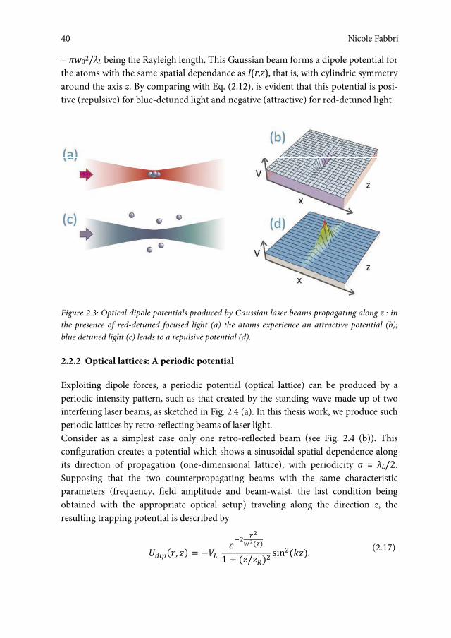
Nicole Fabbri
40
= πw02/λL being the Rayleigh length. This Gaussian beam forms a dipole potential for the atoms with the same spatial dependance as I(r,z), that is, with cylindric symmetry around the axis z. By comparing with Eq. (2.12), is evident that this potential is posi-tive (repulsive) for blue-detuned light and negative (attractive) for red-detuned light.
Figure 2.3: Optical dipole potentials produced by Gaussian laser beams propagating along z : in the presence of red-detuned focused light (a) the atoms experience an attractive potential (b); blue detuned light (c) leads to a repulsive potential (d).
2.2.2 Optical lattices: A periodic potential
Exploiting dipole forces, a periodic potential (optical lattice) can be produced by a periodic intensity pattern, such as that created by the standing-wave made up of two interfering laser beams, as sketched in Fig. 2.4 (a). In this thesis work, we produce such periodic lattices by retro-reflecting beams of laser light. Consider as a simplest case only one retro-reflected beam (see Fig. 2.4 (b)). This configuration creates a potential which shows a sinusoidal spatial dependence along its direction of propagation (one-dimensional lattice), with periodicity a = λL/2. Supposing that the two counterpropagating beams with the same characteristic parameters (frequency, field amplitude and beam-waist, the last condition being obtained with the appropriate optical setup) traveling along the direction z, the resulting trapping potential is described by
������, �� � ��� �����
������ � ��/���� sin
������ (2.17)
Nicole Fabbri40
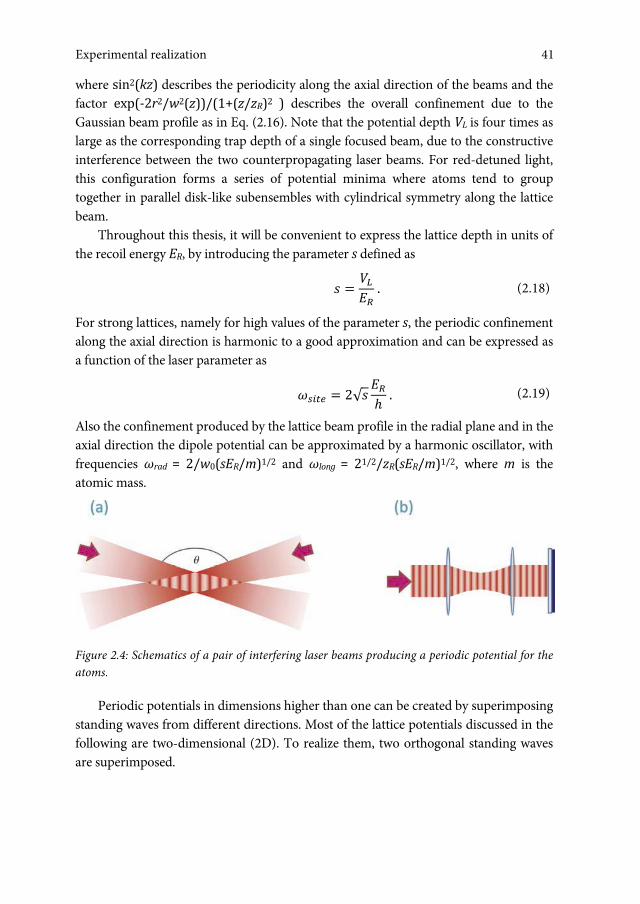
Exploring the superfluid-to-insulator transition in a lattice
41
where sin2(kz) describes the periodicity along the axial direction of the beams and the factor exp(‐2r2/w2(z))/(1+(z/zR)2 ) describes the overall confinement due to the Gaussian beam profile as in Eq. (2.16). Note that the potential depth VL is four times as large as the corresponding trap depth of a single focused beam, due to the constructive interference between the two counterpropagating laser beams. For red-detuned light, this configuration forms a series of potential minima where atoms tend to group together in parallel disk-like subensembles with cylindrical symmetry along the lattice beam.
Throughout this thesis, it will be convenient to express the lattice depth in units of the recoil energy ER, by introducing the parameter s defined as
� � ���� . (2.18)
For strong lattices, namely for high values of the parameter s, the periodic confinement along the axial direction is harmonic to a good approximation and can be expressed as a function of the laser parameter as
����� � 2√� ��� . (2.19)
Also the confinement produced by the lattice beam profile in the radial plane and in the axial direction the dipole potential can be approximated by a harmonic oscillator, with frequencies ωrad = 2/w0(sER/m)1/2 and ωlong = 21/2/zR(sER/m)1/2, where m is the atomic mass.
Figure 2.4: Schematics of a pair of interfering laser beams producing a periodic potential for the atoms.
Periodic potentials in dimensions higher than one can be created by superimposing standing waves from different directions. Most of the lattice potentials discussed in the following are two-dimensional (2D). To realize them, two orthogonal standing waves are superimposed.
41Experimental realization
Nicole Fabbri
42
In principle, the beams cross-interfere between the two different standing waves, owing to a not-perfect linear and mutually orthogonal polarization.8 Undesired cross-interference is typical by prevented by using two different laser frequencies to produce the two standing waves (typically detuned each other by 10 MHz). In that case, the cross-interference term carries a fast-rotating time-phase which does not contribute to the time-averaged effective potential V2D, and the latter is simply given by the sum of those generated by the single stationary waves
�����, �, �� � ����, �, �� � ����, �, �� ≃
��,� sin����� ���,� sin����� � �2 ���
��� � ������������ (2.20)
where x and z denote the directions of propagation of the two stationary waves, and VL,1 = sxER, VL,2 = szER are the corresponding potential depths.
In the presence of such a 2D lattice, atoms are trapped in a 2D array of micro-tubes. For strong enough lattices, i.e., for high values of the two potential depths sx and sz, the transverse dynamics are completely frozen, and atoms can move only along the tube axis. Such a system constitutes our major test-ground to investigate the physics introduced in the first Chapter. More detailed comments on its features will be offered in Sec. 2.3.
Each tube is confined transversally with a trapping frequency given by Eq. (2.19). Moreover, the whole array feels an overall axial and radial confinement with effective trapping frequencies ωx, ωy, and ωz:
��� � �����,�� � ����,�� � � 2��,�� � ����� � � 2
��,��� ����� , (2.21)
��� � ����,�� � �����,�� � � 4��,��
� ����� � � 4
��,��� ����� . (2.22)
where w0,x and w0,z are the minimum waists and zR,x and zR,z are the Rayleigh length of the beams producing the two standing-waves. ωz2 is written in an analogous manner to Eq. (2.20) by inverting x and z. Actually, in the experiment, an additional harmonic confinement is present, due to the magnetic trap where the Bose-Einstein condensate has been produced. The resulting frequency is simply given by the root mean square of the sum of the optical and magnetic squared-frequencies.
8 Moreover, possible time-phase fluctuations induced by the finite coherence-length of the laser source may affect the stability of the periodic potential, since a frequency jitter can induce fluctuations of the node and antinodes positions. This can eventually give rise to decoherence and heating effects of cold atomic samples trapped in the optical potential.
Nicole Fabbri42

Exploring the superfluid-to-insulator transition in a lattice
43
As an extension, a three-dimensional lattice can be formed by overlapping three mutually orthogonal standing-waves. In analogy with the two-dimensional case, near the center of the trap the potential has the form V3D(x,y,z) = VL,x sin2(kx) + VL,y sin2(ky) + VL,z sin2(kz) + m/2(ωx2x2 + ωy2y2 + ωz2z2). If the depth of the potential along each of these axes is the same, atoms arrange themselves in a simple cubic struc-ture. In our experiment instead, the lattice depth is the same along two directions, whereas along the third axis it is set to a variable value, as will be discussed in Sec. 2.4.
2.2.2.1 Experimental realization
Figure 2.5: Scheme of the laser source and the optical system for the control of the frequency and the intensity of the beams used to produce the optical lattices in the experiment.
The laser source. The light source of our optical lattice is a commercial titani-um-sapphire ring laser (Coherent 899-21) pumped by a high-power solid-state fre-quency-doubled laser (Nd-YVO4, Coherent Verdi V18). The pump laser emits about 18 W in single-mode at 532 nm. The gain curve of the active medium of the Ti:Sa laser ranges from 600 nm to 1.10 μm, but the frequency emission is limited to the interval from 760 nm to 850 nm due to the reflectivity of the optical components in
43Experimental realization

Nicole Fabbri
44
the cavity, with a maximum power of 3 W at the center of the gain curve. Sin-gle-mode emission is obtained by means of two etalons with different thickness. A birefringent filter enables us to tune the mode in steps of 0.5 nm. A typical spectral width is less than 1 MHz. The emitted beam has linear polarization with a divergence of 2 mrad. For the experiments performed in the context of this project, the wave-length selected to realize the optical lattices is 830.3 nm, corresponding to a red-detuning of ∼ 20 THz with respect to the D1 and D2 lines of 87Rb.
Figure 2.6: Schematic drawing of the configuration of beams creating the optical lattices with respect to the chamber containing the ultracold sample of 87Rb.
The optical scheme. The laser light originating from the Ti:Sa source is separated in-to three beams by means of λ/2 waveplates and polarization beam splitter cubes, as shown in Fig. 2.5. These beams have linear and mutually orthogonal polarization and are shifted in frequency by 10 MHz relative to each other, in order to avoid cross-interference effects discussed in the previous paragraph. The relative frequency shift is provided by acoustic-optic modulators (AOMs), which also control the laser intensity guaranteeing a fast commutation time in switching on and off (∼ 0.2 μs). A mechanical shutter upstream in the beam line before the separation ensures complete extinction even if has a relatively long light-extinction time (∼ 1 ms). The beam spa-tial mode is filtered by passing through single-mode polarization-maintaining optical fibers. The light intensity of each beam is stabilized by means of a feedback circuit acting on the corresponding AOM driver. The reference signal is provided by inde-pendent generators of arbitrary waveform, which allow us to dynamically change the
Nicole Fabbri44

Exploring the superfluid-to-insulator transition in a lattice
45
potential depths. The feedback signal is obtained by fast photodiodes placed at the output of the fibers, which continuously collect the light from reflections. This system has a short response time (∼ 1 μs), limited by the photodiode bandwidth, and guar-antees a perfect reproducibility of the light intensity used in the experiments, getting rid of fluctuations of the laser source intensity or of the fiber transmittance. Quasi-collimated Gaussian beams come out of the fibers, and are sent to the second vacuum cell (see Sec. 2.1), where the experiments will be conducted, being focused on a degenerate atomic sample. After passing the cell, the beams are again collimated and retroreflected by adjustable mirrors. 8F8F
9 Thus, they follow the inverse paths and produce standing waves (see Fig. 2.6). The measured waists of the lattice beams are wx = (210 ± 3) μm, wx = (160 ± 3) μm, and wx = (190 ± 3) μm, respectively.
Lattice characteristics. The optical lattices we produce have periodicity d = λL/2 = 415 nm; then the atomic cloud occupies roughly 200 lattice sites in the direction along which it is elongated. Actually, the presence of the lattice modifies the size of the cloud. A detailed discussion of how the atoms rearrange in the lattice will be given in Sec. 2.3. For 87Rb, the recoil energy is ER ≃ h × 3.33 kHz and the Bragg velocity, i.e., the velocity acquired by an atom absorbing a photon from the lattice, amounts to ∼ 0.35 mm/s.
The quite large red-detuning of the laser light used for the lattices ensures the light absorption rate to be small, whereby we can consider the optical lattice as a con-servative trapping potential. The heating rate can be estimated as
���� ∼
�����2�
����. (2.23)
Combining Eq. (2.14), (2.17), and (2.18) one can calculate Γsc for a given lattice depth s. In our experiment, for large lattice amplitude, e.g., s = 35, we obtain a heating rate of ∼ 7 nK/s.
Another heating mechanism originates from the time-phase fluctuations. This can be given either by a frequency jitter of the laser source or mechanical noise on the mirror mountings position. Concerning the first contribution, the line-width of the Ti:Sa laser light producing the lattice is about 1 MHz, corresponding to a relative er-ror on the laser wavelength ΔλL/λL ≃ 3 × 10‐9. Since the retro-reflecting mirror is at a distance l ∼ 150 mm ∼ 1.8 × 10⁵ λL from the atomic cloud, after a double passage 2l a phase slip of 2πlΔλL/λL2 ∼ 2 π × 6 × 10‐4 accumulates. This corresponds to a
9 Since the lattice beams are roughly superimposed on the optical path of the second-MOT beams, we use dichroic mirrors which reflect radiation at a wavelength > 800 nm and transmit at 780 nm.
45Experimental realization

Nicole Fabbri
46
very small fluctuation of the nodes and antinodes position, of the order of a half a nanometer, that is 1×10‐3 of the lattice constant. We expect that the most relevant contribution to the heating of the atoms in the optical lattices comes from the me-chanical noise, which is partially healed by using retroreflecting beams to produce the lattice. However, it still constitutes the limiting factor to the lattice stability [82].
2.2.3 Adiabatically loading atoms into a lattice potential
Now we will spend some words on how to put the atoms into the lattice. Once the ensemble of bosons has been driven to the degenerate quantum state of BEC, the laser light is turned on to create the periodic lattice potential, and the atoms spatially reorder to adapt to their new environment. Similarly, the lattice can be removed from the atoms simply by turning off the lasers, thus liberating the atoms into free space once more.
Since we want atoms to change their space-distribution from the harmonic trap into the new periodic trap minimizing the undesired population of excited states, the modification of the external potential must be slow with respect to the typical timescales of the system. In this way, the wave-function of the initial BEC is connected to the many-body ground-state of the gas in the lattice via an adiabatic transformation, to a good approximation. To ensure adiabaticity of the process, three timescales are relevant: One is associated with the energy-gap between different bands, another with the width of the energy bands, and the last with the variation of the chemical potential.
Adiabaticity with respect to vibrational frequencies in the lattice. Fast changes of the lattice amplitude can results in excitations of higher vibrational states of the sys-tem, i.e., higher energy bands of the periodic potential. Considering for simplicity a BEC in a 1D lattice, abruptly switching on the lattice, the momentum state |q will be projected onto a superposition of Bloch quasi-momentum states |n,q belonging to different bands [102] (see Fig. 2.7). To populate a single Bloch state in the lowest band, the transformation must happen on a timescale longer than the inverse of the energy-level spacing. For a non-interacting gas, this condition can be written as [18]
���, �� ���� �0, ��� ������� � ������
� . (2.24)
This time depends on the lattice amplitude. For a non-interacting gas in a weak poten-tial, e.g., s = 1, this time is of the order of 1 ms. As the lattice amplitude increases, the energy gap between different bands grows; thus this adiabaticity condition becomes less stringent.
Nicole Fabbri46

Exploring the superfluid-to-insulator transition in a lattice
47
Figure 2.7: Projection of the momentum state of a non-interacting gas (gray dot on the purple curve) into the quasi-momentum states of a lattice potential. If the loading in the lattice is adia-batic with respect to the vibrational frequencies of the lattice, only the lowest energy band is populated (blue dot), otherwise also higher bands get populated (yellow dots).
Adiabaticity with respect to the quasi-momentum population in the lowest band. In order to allow atoms to redistribute in the ground-state of the lattice, adjusting their momentum distribution, the timescale of the transformation must be longer than the time associated with the bandwidth of the lowest-energy band. Unlike the previous discussion, this condition becomes more stringent as the lattice amplitude grows, since the energy bands flatten. For s = 1, the typical timescale is of the order of 1 ms; for a quite strong lattice, such as s = 5, the typical timescale falls to 4 ms.
Adiabaticity with respect to the modification of the chemical potential. When loading the atoms in a 2D lattice to produce an array of 1D gases, the chemical poten-tial of the cloud changes as we will describe in Sec. 2.3. Now, let us anticipate that for a BEC of 1.2 × 10⁵ atoms and the typical potential we use, μ3D/h ranges from ∼ 0.66 kHz to ∼ 3.2 kHz. The characteristic time for this transformation is again of the order of 1 ms.
In the experiment, in order to fulfil the conditions above, the laser light intensity – which the lattice amplitude is proportional to – is progressively increased up to its final amplitude. The shape and the timing of the intensity sweep have been optimized as follows. We load a pure 3D BEC in the lattices with a trial ramp, then perform the reverse process ramping-down the lattices, wait half a second for letting the gas to
47Experimental realization

Nicole Fabbri
48
rethermalize and finally measure the condensed fraction of the atomic cloud. The re-duction of the condensed fraction gives an estimate of the amount of undesired exci-tations produced in the many-body state realized in the lattices. As a result of this op-timization, we adopt a 140 ms-long exponential ramp with time constant τ = 30 ms.
2.3 Realizing an array of 1D gases
In our experiments, we realize a two-dimensional array of about 2 × 10³ one-dimensional atomic micro-tubes. To arrange atoms in this configuration, we start from a three-dimensional degenerate gas of ∼ 1.2 × 10⁵ atoms of 87Rb in the magnetic trap. Then, we confine it in a pair of strongly-confining and orthogonal optical lattices aligned along the axes x and z, having the same amplitude sx = sz ≡ s.
Unlike alternative realization of the 1D physics, such as in chip experiments (e.g., in [103]), where transverse trapping frequencies hardly exceed a few kHz and are typically of the order of the chemical potential and the temperature, optical lattices provide a much stronger transverse confinement [104, 33]. The drawback of the latter system is that one obtains a large number of different 1D tubes, and this makes the description of the system more complicated.
For this purpose, we developed a model at zero temperature that allows us to calculate how atoms rearrange in the array of tubes created by the two orthogonal optical lattices. This is based on the theoretical work by Krämer et al. [55] on a system in a 1D lattice, and extends it to a 2D lattice. From our model, we extract the crucial quantities which describe our system, such as the density and the chemical potential. The key concepts and the results of our calculation are presented in the next Section.
2.3.1 Atom distribution in the array
Let us start by considering a three-dimensional Bose-Einstein condensate of N = 1.2 × 10⁵ atoms, as we typically realize in the experiments. It corresponds to a chemical potential μ3D/h ≃ 0.66 kHz, and a total size of ≃ 9.6 μm × 96 μm, the aspect ratio being determined by the trap. When ramping up the 2D optical lattices, the potential felt by the atoms is given by the sum of the 3D harmonic trap and the optical confinement. The optical lattices introduce two important effects. (i) The kinetic energy term in the transverse plane has no longer the classical quadratic form as in the radial direction, but exhibits a periodic dependence on the gradient of the phase. (ii) The interaction coupling constant is renormalized due to the presence of the optical lattice. This results from the local compression of the gas produced by the tight optical confinement which enhances the repulsive effect of the interactions. As a result of these effects, the radial density profile is modulated with the periodicity of the lattice constant
Nicole Fabbri48
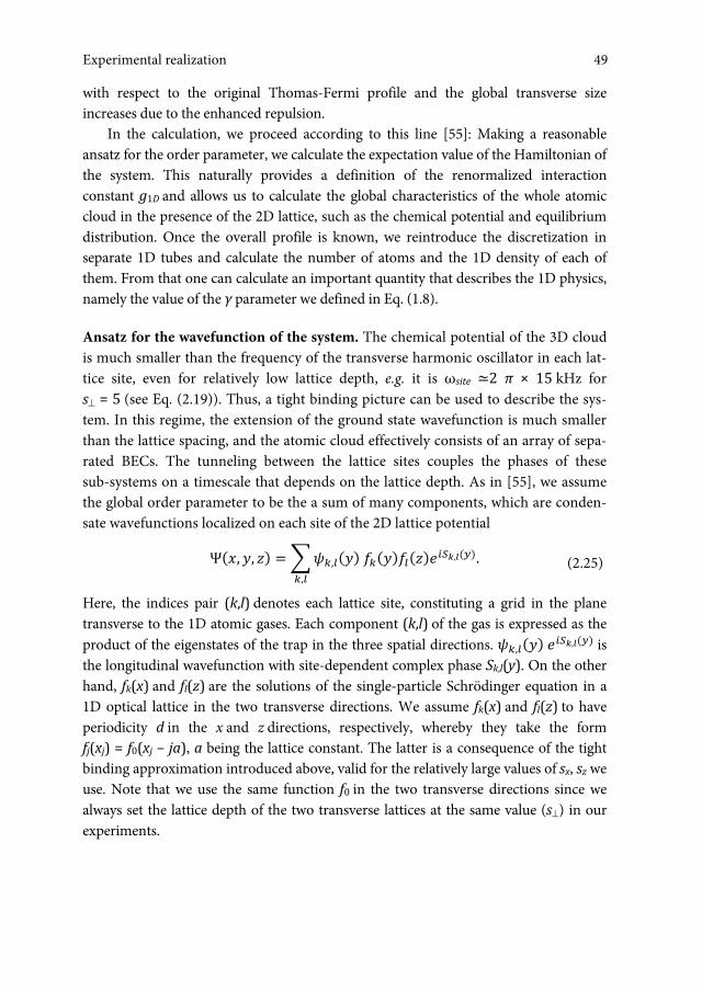
Exploring the superfluid-to-insulator transition in a lattice
49
with respect to the original Thomas-Fermi profile and the global transverse size increases due to the enhanced repulsion.
In the calculation, we proceed according to this line [55]: Making a reasonable ansatz for the order parameter, we calculate the expectation value of the Hamiltonian of the system. This naturally provides a definition of the renormalized interaction constant g1D and allows us to calculate the global characteristics of the whole atomic cloud in the presence of the 2D lattice, such as the chemical potential and equilibrium distribution. Once the overall profile is known, we reintroduce the discretization in separate 1D tubes and calculate the number of atoms and the 1D density of each of them. From that one can calculate an important quantity that describes the 1D physics, namely the value of the γ parameter we defined in Eq. (1.8).
Ansatz for the wavefunction of the system. The chemical potential of the 3D cloud is much smaller than the frequency of the transverse harmonic oscillator in each lat-tice site, even for relatively low lattice depth, e.g. it is ωsite ≃2 π × 15 kHz for s = 5 (see Eq. (2.19)). Thus, a tight binding picture can be used to describe the sys-tem. In this regime, the extension of the ground state wavefunction is much smaller than the lattice spacing, and the atomic cloud effectively consists of an array of sepa-rated BECs. The tunneling between the lattice sites couples the phases of these sub-systems on a timescale that depends on the lattice depth. As in [55], we assume the global order parameter to be the a sum of many components, which are conden-sate wavefunctions localized on each site of the 2D lattice potential
��, �, �� ����,���� ��������������,�����,�
. (2.25)
Here, the indices pair (k,l) denotes each lattice site, constituting a grid in the plane transverse to the 1D atomic gases. Each component (k,l) of the gas is expressed as the product of the eigenstates of the trap in the three spatial directions. ��,���� ����,���� is the longitudinal wavefunction with site-dependent complex phase Sk,l(y). On the other hand, fk(x) and fl(z) are the solutions of the single-particle Schrödinger equation in a 1D optical lattice in the two transverse directions. We assume fk(x) and fl(z) to have periodicity d in the x and z directions, respectively, whereby they take the form fj(xj) = f0(xj – ja), a being the lattice constant. The latter is a consequence of the tight binding approximation introduced above, valid for the relatively large values of sx, sz we use. Note that we use the same function f0 in the two transverse directions since we always set the lattice depth of the two transverse lattices at the same value (s) in our experiments.
49Experimental realization

Nicole Fabbri
50
Mean-field expectation value of the Hamiltonian. Using the ansatz in Eq. (2.25) for the order parameter, we calculate the mean field expectation value of the effective Hamiltonian
� ������
2� � ����������
� ������ � ����
. (2.26)
Here, g = 4π �2/as is the coupling constant of the 3D gas, and Vext is the sum of the magnetic and optical external potential, and can be conveniently separated into a slow-varying harmonic trapping due to the magnetic trap and the gaussian profile of the lattice beams, plus the axial periodic confinement in the lattice sites.
After some manipulation of the terms composing the Hamiltonian,10 we trans-form the discrete formalism used in Eq. (2.26) into continuum variables, as in Ref. [55]. This will allow us to discuss the macroscopic properties of the system. This pro-cedure naturally introduces a smoothed macroscopic density defined by
��� � ��� �� � � ��� � ����� ���� . (2.27)
The expectation value of the Hamiltonian gives
� � ��� �� �� �� ����� ��2 � ��� � �� � �������2� � ���������
2� �
− ∫ �� �� �� �0[�1 cos(����) � �2 cos(����)] (2.28)
Here, we have introduced the renormalization cupling constant
���� � � �� ��� ��� � �� ��� . (2.29)
To express ���� as a function of the lattice parameter, we calculate f0 as the ground-state solution of the stationary Schroedinger equation for the transverse motion in one dimension, i.e., single-site Wannier function. In addition, we approximate the single-site potential by a series of harmonic wells, thus the single-site Wannier func-tion is reduced to the lowest-energy eigenstate of the harmonic oscillator.
10 We calculate separately the expectation value of the kinetic energy, the external trapping potential and the atom-atom interaction energy. For the kinetic energy, we take into account the contribution of a sin-gle lattice site to the transverse kinetic energy, and the on-site axial kinetic energy. We consider separately the contributions of the wavefunction overlap of two consecutive wells (namely, two contigouos gases) to the lattice trap potential and to the radial kinetic energy. Instead, as in [55] we neglect the contribution of neighbours sites on the axial kinetic energy and on the potential energy associated with the harmonic trap, as well as the wavefunction overlap between lattice sites more distant than the nearest neighbours. Finally, we neglected a quantum pressure term originating from the radial term in the kinetic energy.
Nicole Fabbri50
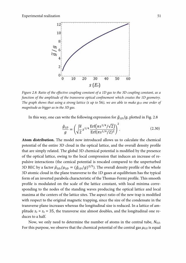
Exploring the superfluid-to-insulator transition in a lattice
51
Figure 2.8: Ratio of the effective coupling constant of a 1D gas to the 3D coupling constant, as a function of the amplitude of the transverse optical confinement which creates the 1D geometry. The graph shows that using a strong lattice (s up to 56), we are able to make g1D one order of magnitude as bigger as in the 3D gas.
In this way, one can write the following expression for ����/g, plotted in Fig. 2.8
����� � ���2 �
�/� Erf����/�/√2�Erf����/�/2�� �
�. (2.30)
Atom distribution. The model now introduced allows us to calculate the chemical potential of the entire 3D cloud in the optical lattice, and the overall density profile that are simply related. The global 3D chemical potential is modified by the presence of the optical lattice, owing to the local compression that induces an increase of re-pulsive interactions (the cemical potential is rescaled compared to the unperturbed 3D BEC by a factor ����/��� � �����/���/�). The overall density profile of the whole 3D atomic cloud in the plane transverse to the 1D gases at equilibrium has the typical form of an inverted parabola characteristic of the Thomas-Fermi profile. This smooth profile is modulated on the scale of the lattice constant, with local minima corre-sponding to the nodes of the standing waves producing the optical lattice and local maxima at the centers of the lattice sites. The aspect ratio of the new trap is modified with respect to the original magnetic trapping, since the size of the condensate in the transverse plane increases whereas the longitudinal size is reduced. In a lattice of am-plitude sx = sz = 35, the transverse size almost doubles, and the longitudinal one re-duces to a half.
Now, we only need to determine the number of atoms in the central tube, N0,0. For this purpose, we observe that the chemical potential of the central gas μ0,0 is equal
51Experimental realization

Nicole Fabbri
52
to the chemical potential of the whole gas. From Eq. (1.15), the number of atoms of the central gas is
��,� � 2���3
��,�������������
. (2.31)
The number of atoms in each tube labeled (k,l) is distributed according to
��,� � ��,� �1 � �� � ������� �
�. (2.32)
where kmax is the Thomas-Fermi transverse radius of the overall distribution, in units of the lattice constant a, whichcan be simply derived from the modified chemical po-tential ����. These relations completely determine how the atoms distribute in the ar-ray, given the total number of atoms of the 3D gas and the trapping frequencies of the magnetic and optical confinement. From that, several important quantities, such as the chemical potential and density of each 1D gas can be calculated. For example, the ratio between interaction and kinetic energy can be easily calculated according to � � ����������,��� � 0��, where ��,��� � 0� is the density of the tube labeled (k,l) in its center.
Finally, the inhomogeneity of the 1D gases along their axial direction must be considered. The numerical solution of the Non-Polynomial Schroedinger equation (NPSE) performed with our experimental parameters [105] has demonstrated that the longitudinal density-profile of the 1D gases is very close to a 1D Thomas-Fermi profile (no difference is observed within the numerical errors). In the following, we will assume that this is indeed the case, and accordingly we define the axial Thomas-Fermi radius
�����,� � � ���,�����. (2.33)
Typically, one can evaluate the atom distribution in the 2D lattice for given am-plitude of the 2D optical lattice, assuming the distribution to be frozen due to a small tunneling rate from one site to the other. With this prospect, we calculate the main parameters which define the array of 1D tubes using the previous procedure, for a fixed total number of atoms N = 1.2 × 10⁵ for different lattice depth s. Table 2.1 re-ports the number of atoms in the 1D gas which occupies the central site N0,0, its 1D chemical potential �� in units of h and its Thomas-Fermi radius along its axial direc-tion, as well as the value of the parameter γ averaged over the ensemble and the inter-atomic coupling constant ���� of the whole gas.
Nicole Fabbri52
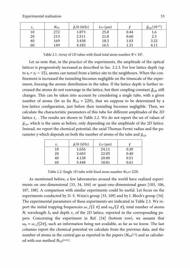
Exploring the superfluid-to-insulator transition in a lattice
53
s N0,0 ��/� (kHz) LTF (μm) �̅ ����(10‐37) 10 20 40 60
272 213 169 149
1.8732.511 3.438 4.183
25.821.8 18.3 16.5
0.440.68 1.03 1.31
1.6 2.3 3.32 4.11
Table 2.1: Array of 1D tubes with fixed total atom number N = 105.
Let us note that, in the practice of the experiments, the amplitude of the optical lattices is progressively increased as described in Sec. 2.2.3. For low lattice depth (up to sx = sz ∼ 15), atoms can tunnel from a lattice site to the neighbours. When the con-finement is increased the tunneling becomes negligible on the timescale of the exper-iment, freezing the atomic distribution in the tubes. If the lattice depth is further in-creased the atoms do not rearrange in the lattice, but their coupling constant ���� still changes. This can be taken into account by considering a single tube, with a given number of atoms (let us fix N0,0 = 220), that we suppose to be determined by a low-lattice configuration, just before then tunneling becomes negligible. Then, we calculate the characteristic parameters of this tube for different amplitudes of the 2D lattice s . The results are shown in Table 2.2. We do not report the set of values of ����, which is the same as before, only depending on the amplitude of the 2D lattice. Instead, we report the chemical potential, the axial Thomas-Fermi radius and the pa-rameter γ which depends on both the number of atoms of the tube and ����.
s ��/� (kHz) LTF (μm) �̅1020 40 60
1.6562.603 4.138 5.448
24.1122.05 20.00 18.81
0.300.40 0.51 0.61
Table 2.2: Single 1D tube with fixed atom number N0,0= 220.
As mentioned before, a few laboratories around the world have realized experi-ments on one-dimensional [33, 34, 104] or quasi-one-dimensional gases [103, 106, 107, 108]. A comparison with similar experiments could be useful. Let focus on the experiments conducted by D. S. Weiss's group [33, 109] and by I. Bloch's group [34]. The experimental parameters of these experiments are indicated in Table 2.3. We re-port the initial trapping frequencies ω/(2 π) and ωy/(2 π), total number of atoms N, wavelength λL and depth s of the 2D lattice, reported in the corresponding pa-pers. Concerning the experiment in Ref. [34] (bottom row), we assume that ωy = ω/(2π), such an information being not available, as far as we know. The last columns report the chemical potential we calculate from the previous data, and the number of atoms in the central gas as reported in the papers (N0,0(r.)) and as calculat-ed with our method N0,0(o.m.).
53Experimental realization
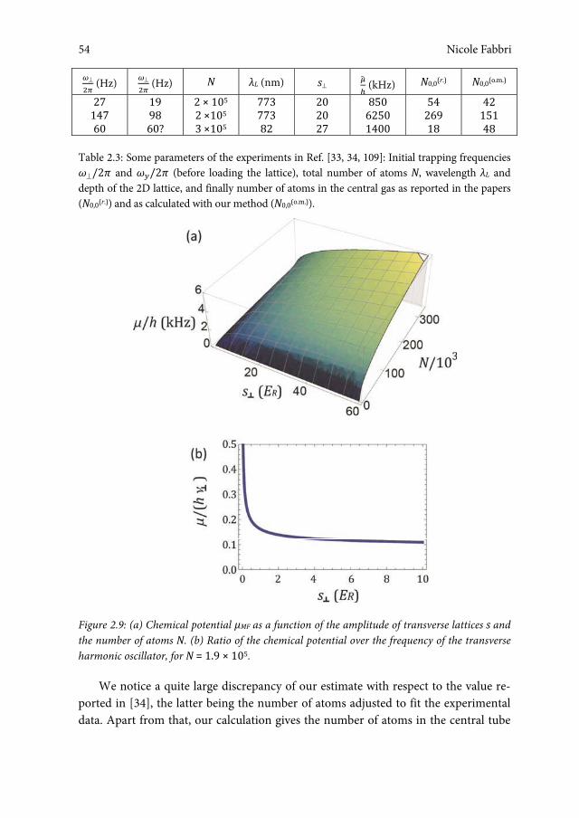
Nicole Fabbri
54
�
�� (Hz) �
�� (Hz) N λL (nm) s ��� (kHz) N0,0(r.) N0,0(o.m.)
27 147 60
19 98 60?
2 × 10⁵ 2 ×10⁵ 3 ×10⁵
773773 82
2020 27
8506250 1400
54 269 18
42151 48
Table 2.3: Some parameters of the experiments in Ref. [33, 34, 109]: Initial trapping frequencies ��2� and ���2� (before loading the lattice), total number of atoms N, wavelength λL and depth of the 2D lattice, and finally number of atoms in the central gas as reported in the papers (N0,0(r.)) and as calculated with our method (N0,0(o.m.)).
Figure 2.9: (a) Chemical potential μMF as a function of the amplitude of transverse lattices s and the number of atoms N. (b) Ratio of the chemical potential over the frequency of the transverse harmonic oscillator, for N = 1.9 × 10⁵.
We notice a quite large discrepancy of our estimate with respect to the value re-ported in [34], the latter being the number of atoms adjusted to fit the experimental data. Apart from that, our calculation gives the number of atoms in the central tube
Nicole Fabbri54

Exploring the superfluid-to-insulator transition in a lattice
55
close to the value reported in these papers, which makes us confident of the validity of our estimate.
2.3.2 Some numbers for our 1D gases
Now, we will summarize the main characteristics of our ensemble of 1D gases, extracted from the model we developed in the previous section. For all amplitudes of the transverse lattice we explore in the experiment (s ≥ 5) the system has a 1D character, i.e., all energy scales are much smaller than the single-particle level spacing in the potential wells; more particularly, the relevant energy scales are thermal energy kBT and chemical potential μ. In the case of large potential barriers the transverse confinement is well approximated by a harmonic oscillator and the level spacing is given by �.
Concerning the chemical potential, for the employed parameters (atomic mass and trapping frequencies) the 3D gas has typically μ/h less than 1 kHz, with a weak dependence on the total number of atoms (μ ∝ N2/5). In the presence of a lattice, the chemical potential depends on the amplitude of the lattices which confines the gas in a 1D geometry as well. Its behaviour is represented in Fig. 2.9 (a). For s ≥ 1, the chemical potential is about one order of magnitude less than � (the latter increasing as s1/2), as shown in Fig. 2.9 (b)).
Concerning temperature, we expect it does not exceed ∼ 100 – 200 nK, corre-sponding to a few kHz. In fact, as a general point, we verified the 1D gases to be su-perfluid, by measuring the ratio between the frequency of the breathing mode ωB/(2π) to the dipole mode ωD/(2π) [110, 111]. Indeed the ratio of these frequen-cies is ωB/ ωD = 31/2 for a Bose condensed gas, whereas ωB/ωD = 2 for a thermal cloud. We have measured this ratio as a function of the time spent by the gas in the 2D optical lattice, with the results shown in Fig. 2.10.
For holding times in the 2D lattice up to 50 ms (at s = 35), this ratio is close to the value 31/2 corresponding to the expected value for 1D Bose-condensed gases close to the mean-field regime [110, 111]. For longer holding times, the ratio increases up to the value 2 expected for a thermal 1D Bose gas.
All the experiments we will discuss are performed with a typical holding time of 10 ms at the amplitude s = 35 ensuring the 1D gases are Bose-condensed. This ensures the temperature is lower than the critical value (∼ 125 nK). Considering a trial temperature of 150 nK, for s > 10 the population of the first-excited state of the transverse harmonic oscillator is about 0.002 of the ground-state population. For s = 20 it falls to 3 × 10‐6. The calculation has been performed using the Bose-Einstein distribution (cfr. Fig. 2.11).
55Experimental realization
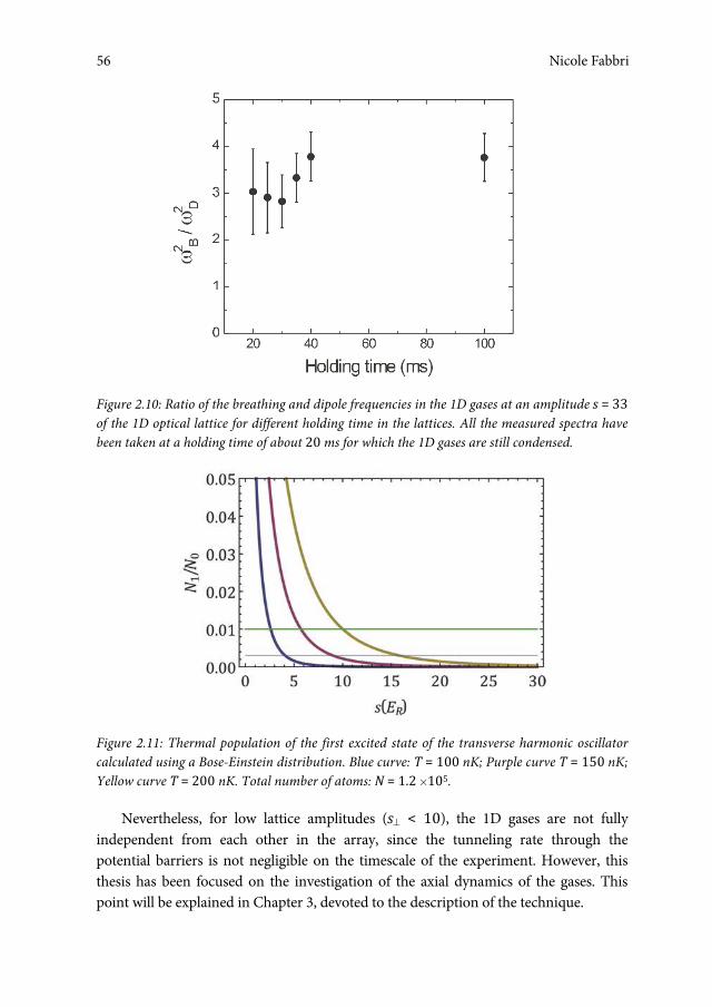
Nicole Fabbri
56
Figure 2.10: Ratio of the breathing and dipole frequencies in the 1D gases at an amplitude s = 33 of the 1D optical lattice for different holding time in the lattices. All the measured spectra have been taken at a holding time of about 20 ms for which the 1D gases are still condensed.
Figure 2.11: Thermal population of the first excited state of the transverse harmonic oscillator calculated using a Bose-Einstein distribution. Blue curve: T = 100 nK; Purple curve T = 150 nK; Yellow curve T = 200 nK. Total number of atoms: N = 1.2 H105.
Nevertheless, for low lattice amplitudes (s < 10), the 1D gases are not fully independent from each other in the array, since the tunneling rate through the potential barriers is not negligible on the timescale of the experiment. However, this thesis has been focused on the investigation of the axial dynamics of the gases. This point will be explained in Chapter 3, devoted to the description of the technique.
Nicole Fabbri56

Exploring the superfluid-to-insulator transition in a lattice
57
Figure 2.12: (a) On-site interaction energy U, (b) tunneling energy J and (c) ratio U/J. These quantities are reported as functions of the longitudinal lattice amplitude sy.
2.4 Realizing the superfluid-to-insulator transition
A substantial part of the work of this thesis has been devoted to the investigation of the physics of 1D gases in the presence of a periodic potential along their axis (see Chapters 5 and 6). This kind of system is a realization of the Bose-Hubbard model we presented in Sec. 1.4. In the following, we would like to give some details about our realization of such systems and illustrate how the experimental parameters are related to the key physical quantities.
In practice, we start from an array of 1D gases produced by tightly confining a 3D gas in a strong 2D lattice with amplitude s = 35 and wavelength λL = 830 nm, as illustrated in the previous Section. To this system we add another 1D optical lattice along the axial direction of the micro-tubes, with the same wavelength as the transverse lattices but with variable amplitude.
The relative strength of the on-site interaction energy U with respect the tunneling J along the axes of the tubes is controlled by the depth V0 of the periodic potential superimposed along the axial direction. In Ref. [112] these quantities are evaluated by
57Experimental realization

Nicole Fabbri
58
approximating the single-site wavefunction with a Gaussian profile. A more accurate estimate can be obtained by numerically evaluating the Wannier wavefunctions – which are the correct eigenstates of the Bose-Hubbard Hamiltonian – and performing a fit to the calculated curves, as in Ref. [40]. From the definition given in Eq. (1.24) and (1.23), respectively, one gathers simple equations which express the dependence of U and J on the lattice amplitude:
��� � ���� ���� ���
� ��� �����
(2.34)
���� � 1�4���������������� (2.35)
Equations (1.28) and (1.29) clearly indicate that the parameters U and J can be varied continuously by tuning the lattice amplitude, as illustrated in Fig. 2.12 (a) and 2.12 (b). Fig. 2.12 (c) reports the ratio U/J, which governs the behaviour of the sys-tem, driving the transition from superfluid to Mott insulator.
2.4.1 Measuring the momentum distribution across the transition
The momentum distribution of a lattice gas can be simply measured by imaging the density distribution after time-of-flight. Figure 2.13 describes the procedure used in the experiment. The light intensity of the lattice is slowly increased with a ramp of 140 ms, then after a holding time in the lattice of 7 ms the optical and magnetic potentials are suddenly switched off simultaneously. The atomic cloud is allowed to fall under gravity, during a typical time-of-flight of 21 ms. Then the cloud is observed via absorption imaging in the plane y–z as described in Sec. 2.1.1. Two representative images are reported in Fig. 2.14(a) and (b) for sy = 0 and sy = 14, respectively.
Figure 2.13: Experimental protocol used to measure the momentum distribution of a lattice gas.
Let us focus for the moment on image 2.14 (a), which shows the BEC emitted from an array of trapped 1D gas as without any periodic potential. The density profile
Nicole Fabbri58
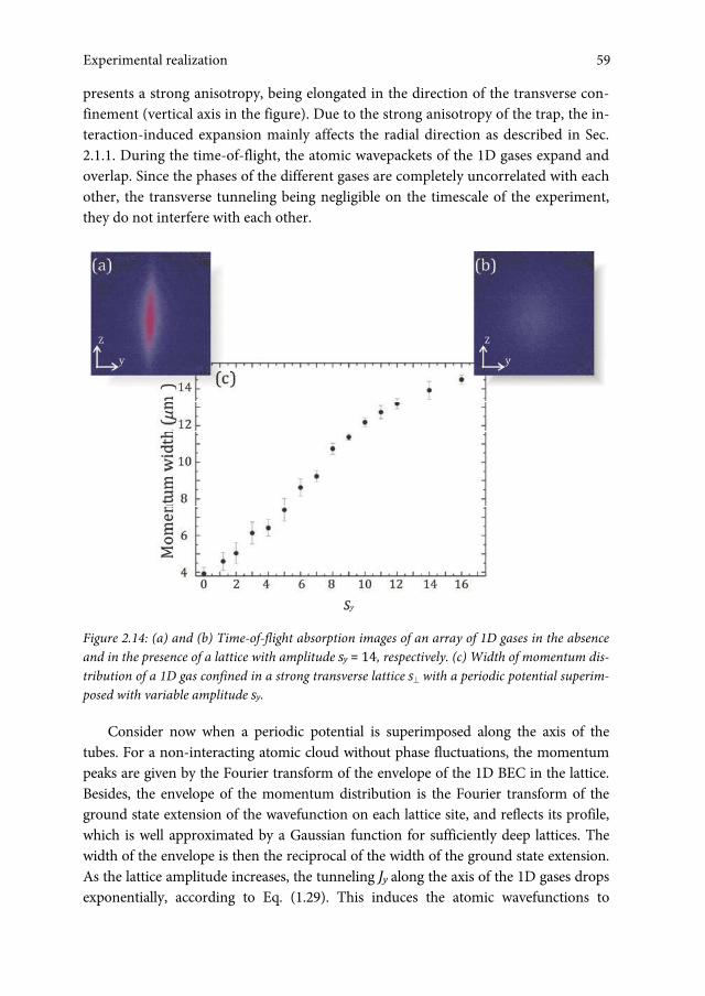
Exploring the superfluid-to-insulator transition in a lattice
59
presents a strong anisotropy, being elongated in the direction of the transverse con-finement (vertical axis in the figure). Due to the strong anisotropy of the trap, the in-teraction-induced expansion mainly affects the radial direction as described in Sec. 2.1.1. During the time-of-flight, the atomic wavepackets of the 1D gases expand and overlap. Since the phases of the different gases are completely uncorrelated with each other, the transverse tunneling being negligible on the timescale of the experiment, they do not interfere with each other.
Figure 2.14: (a) and (b) Time-of-flight absorption images of an array of 1D gases in the absence and in the presence of a lattice with amplitude sy = 14, respectively. (c) Width of momentum dis-tribution of a 1D gas confined in a strong transverse lattice s with a periodic potential superim-posed with variable amplitude sy.
Consider now when a periodic potential is superimposed along the axis of the tubes. For a non-interacting atomic cloud without phase fluctuations, the momentum peaks are given by the Fourier transform of the envelope of the 1D BEC in the lattice. Besides, the envelope of the momentum distribution is the Fourier transform of the ground state extension of the wavefunction on each lattice site, and reflects its profile, which is well approximated by a Gaussian function for sufficiently deep lattices. The width of the envelope is then the reciprocal of the width of the ground state extension. As the lattice amplitude increases, the tunneling Jy along the axis of the 1D gases drops exponentially, according to Eq. (1.29). This induces the atomic wavefunctions to
59Experimental realization

Nicole Fabbri
60
localize more tightly in the single lattice sites. Thus, the phase-coherence between different lattice sites of the same 1D gas is reduced, and a larger momentum distribution after time-of-flight gets populated. As a matter of fact, the image in Fig. 2.14(b) shows that the momentum distribution of the system immersed in a strong lattice is remarkably larger than in the absence of the lattice. We also performed a systematic analysis of the momentum distribution of the array of 1D gases in the presence of a lattice potential along their axial direction. We started from a superfluid and progressively increased the raising the lattice depth, up to enter a Mott insulating state. From the images of the density profile of the atomic cloud, we extracted the width of the momentum distribution, which monotonically increases as displayed in Fig. 2.14(c), according to the arguments presented above.
2.5 Conclusions
In this Chapter we have presented the main ingredients used in the project developed for this thesis: The Bose-Einstein condensate and the optical lattices. These tools enable us to realize a formidable test ground to investigate the physics of 1D systems, both in a continuum space and in a discrete lattice. In Sec. 2.3, we discussed the main characteristics of the array of 1D gases we realized, obtained by developing a theoretical model which extends the work in [55], as well as the features of these gases in the presence of a periodic lattice along their axis.
Nicole Fabbri60

Chapter 3 Spectroscopy via inelastic light scattering
From the experimental point of view, a crucial step in characterizing complex quantum phases consists in finding ways to measure the low-energy excitations of many-body systems, the knowledge of which is fundamental, since they account for the response of the system to a weak perturbation. In the context of condensed-matter physics, the development of angle-resolved photoemission spectroscopy has played a major role in the study of high-Tc superconductors giving information about the one-particle spectral function [113]. More generally, scattering light or particles off solids provided some of the most fundamental insights into the structure of matter [114, 115]. It allowed the measurement of the low-energy excitation spectrum, giving access to the dispersion relations of phonons and the electronic band structure, which can tell in most cases if the material is a metal or an insulator. Now, inelastic light scattering is a natural candidate also to investigate the correlated quantum phases we realized with ultracold atomic gases, where solid-state physics problems are addressed from a different perspective [43]. This Chapter is intended to show how inelastic-light scattering (also known as Bragg scattering) provides a measurement of the correlation functions of the system, describing low-energy excitations. General aspects of Bragg scattering are introduced, both in terms of diffraction from a periodic structure and in terms of two-photon transition, indicating its suitability as an effective spectroscopic technique. The basics concepts of linear-response theory are approached, and discussed how the dynamical structure function and one-particle spectral function are accessible via Bragg scattering in different ranges of parameters. Finally, the experimental setup built for this purpose and the measurement procedure are presented in detail. The quantity accessible in practice is related to the energy absorbed by the gas, and the conditions necessary to guarantee the linearity of the response are examined.
3.1 Generalities about Bragg scattering
In 1912 W. H. Bragg demonstrated backward-scattering of X-rays from a crystal planes, so-called Bragg scattering. In the context of cold atoms, the complementary process is
Nicole Fabbri, Bragg spectroscopy of quantum gases: Exploring physics in one dimension isBN 978-88-6655-220-8 (print) isBN 978-88-6655-221-5 (online) © 2012 Firenze University Press

Nicole Fabbri
62
realized: Rather than diffracting light on a grating of atoms, atoms are diffracted on a grating of coherent light.
In the 1980s, the first experiments were performed letting an atomic beam cross a light grating made up of a static optical lattice [116, 117, 118]. In perfect analogy with the solid-state counterpart, the process is efficient if the incident beam satisfies the Bragg condition on the angle of incidence. Later on, a more convenient experimental configuration has ended up prevailing: Atoms at rest are diffracted by a moving optical lattice created by two intersecting laser pulses with different frequencies. Bragg scattering was used for the first time in 1994 to impart momentum to different velocity classes of a thermal cloud of laser-cooled atoms [119] and in 1999 by the group of Phillips at NIST to impart momentum to a Bose-condensed cloud of atoms [120], and to coherently split the cloud in momentum space. In contrast to the diffraction of an atomic beam, the interaction time is no long determined by the passage of the atoms through a standing wave, but by the duration of the laser pulse. In addition, the condition on the angle of incidence becomes a condition on the frequency difference between the two beams comprising the standing wave, or equivalently, the velocity of the moving standing wave. More precisely, this process occurs as long as the energy and momentum transferred to the condensate match the energy and momentum of the moving optical lattice. Such anenergy is determined by the frequency difference between the beams, and the lattice momentum qB is determined by the beams angle of intersection, as we will see in detail in Sec. 3.1.2.
Since Bragg diffraction provides efficient, selectable momentum and energy transfer, it can be used as an effective tool for spectroscopy, referred to as Bragg spectroscopy. This technique has been applied in pioneering experiments to measure the dynamic structure factor of gaseous Bose-Einstein condensates [121, 122]. The response of the condensate to Bragg transitions of different frequencies provided a spectroscopic measurement of the Bogoliubov excitation energy. The dispersion relation of interacting BECs in the mean-field regime [123, 124, 125], the presence of phase fluctuations in elongated BECs [107] as well as signatures of vortices [126] have been investigated using this technique. Bragg spectroscopy has been also used as a tool to coherently manipulate atomic clouds for interferometric schemes [127] or for thermodynamics studies [128]. More recently it has succeeded in providing novel information about strongly interacting 3D Bose [48] and Fermi [49] gases close to Feshbach resonances.
As soon as experiments on ultracold quantum gases in optical lattices started to simulate many-body systems, theoretical papers appeared proposing to measure their dynamical structure factor through inelastic light scattering [129, 130, 131]. This has been realized in this thesis work to characterize weakly interacting BECs in periodic potentials [132], as well as in the works of Du et al. [51] and Ernst et al. [52] using different configurations of the optical lattices. Moreover, we have exploited Bragg
Nicole Fabbri62
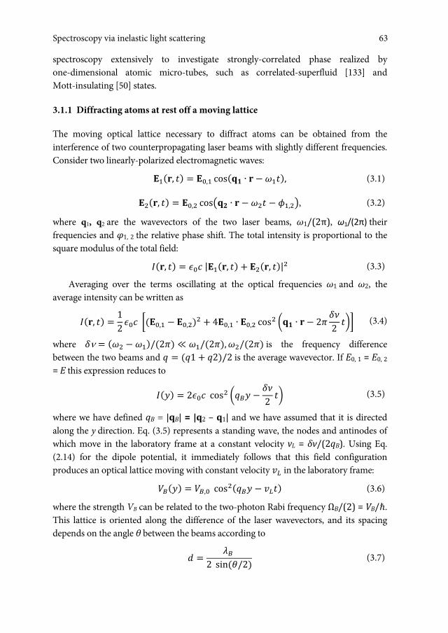
Exploring the superfluid-to-insulator transition in a lattice
63
spectroscopy extensively to investigate strongly-correlated phase realized by one-dimensional atomic micro-tubes, such as correlated-superfluid [133] and Mott-insulating [50] states.
3.1.1 Diffracting atoms at rest off a moving lattice
The moving optical lattice necessary to diffract atoms can be obtained from the interference of two counterpropagating laser beams with slightly different frequencies. Consider two linearly-polarized electromagnetic waves: ����, �� � ��,� cos��� � � � ����, (3.1)
����, �� � ��,� cos��� � � � ��� � ��,��, (3.2)
where q1, q2 are the wavevectors of the two laser beams, ω1/(2π), ω1/(2π) their frequencies and φ1, 2 the relative phase shift. The total intensity is proportional to the square modulus of the total field:
���, �� � ��� |����, �� � ����, ��|� (3.3)
Averaging over the terms oscillating at the optical frequencies ω1 and ω2, the average intensity can be written as
���, �� � 12 ��� ����,� � ��,��� � ���,� � ��,� cos� ��� � � � 2� ��2 ��� (3.4)
where � � ��� � ���/�2�� � ��/�2��,��/�2�� is the frequency difference between the two beams and � � ��1 � �2�/2 is the average wavevector. If E0, 1 = E0, 2 = E this expression reduces to
���� � 2��� cos� ���� � ��
2 �� (3.5)
where we have defined qB = |qB| = |q2 – q1| and we have assumed that it is directed along the y direction. Eq. (3.5) represents a standing wave, the nodes and antinodes of which move in the laboratory frame at a constant velocity vL = δν/(2qB). Using Eq. (2.14) for the dipole potential, it immediately follows that this field configuration produces an optical lattice moving with constant velocity �� in the laboratory frame: ����� � ��,� cos����� � ���� (3.6)
where the strength VB can be related to the two-photon Rabi frequency ΩB/(2) = VB/�. This lattice is oriented along the difference of the laser wavevectors, and its spacing depends on the angle θ between the beams according to
� � ��2 s����/2� (3.7)
63Spectroscopy via inelastic light scattering

Nicole Fabbri
64
λB being the wavelength of the two Bragg beams creating the lattice.
3.1.2 Two-photon Bragg transition Scattering of light by atoms in the Bragg regime can be viewed also as a two-photon transition between two different momentum states of the same internal ground-state [120]: The gas is shone with two simultaneous off-resonant light pulses (Bragg beams) for a finite time tB, with a relative angle θ and detuned from each other by the tunable frequency-difference δv above defined. During the Bragg pulse, atoms absorb photons from one beam and are stimulated to emit photons in the second beam, crossing a virtual state (see gray arrows in Fig. 3.1 (a)). The initial and final momentum states (denoted by open circles in Figure) form an effective two-level system coupled by a two-photon Raman process (red arrow in Figure). As anticipated above, the transition is resonant provided that energy and momentum are conserved. Atoms with initial momentum pi end up in the same internal state with a final momentum pf = pi + �qB, where �qB is the momentum transfer given by the two-photon process. The energy difference between the initial and final atomic states is given by the frequency-difference between the two Bragg beams (�ω = h δv).
In contrast to angle-resolved photoemission spectroscopy, the momentum �qB is directly imprinted on the sample; it is set by the wavelength λB of the Bragg beams and is freely variable by changing the angle θ between them. Namely it is defined as
��� � �� ��� ��� ��2� �
e�� � e���e�� � e��� (3.8)
where eq1, eq2 are the unit vectors of the two beams. Note that the direction of qB is perpendicular to the bisector between the two beams. The detuning δv between the two Bragg beams controls not only the energy �ω transferred to the atoms but also the sign of the momentum transfer. For a two-photon transition towards an excited state with higher kinetic energy, atoms absorb a photon from the beam with the higher-energy photons and are stimulated to emit a photon in the beam with the lower-energy photons. Therefore, with our convention, when the detuning δv is positive atoms absorb photons from beam (1), emit into beam (2) and the momentum transfer is ��qB (dark-gray dashed line in Fig. 3.1 (a)). When δv is negative atoms absorb from beam (2), emit into beam (1) and the momentum transfer is opposite, i.e., ��qB (light-gray dashed line in Fig. 3.1 (a)).
By scanning the relative detuning of the two Bragg beams (and thus the energy of the excitation created in the system) at fixed momentum transfer qB, as sketched by the vertical dotted line in Fig. 3.1 (a), one can monitor the energy absorbed by the system (the method is described in detail in Sec. 3.3.2). When the energy of the excita-tion matches the resonance energy of the system, the absorption is efficient.
Nicole Fabbri64

Exploring the superfluid-to-insulator transition in a lattice
65
Figure 3.1: (a) Schematics of Bragg transitions for a free particle. The atom, considered initially at rest for simplicity, is illuminated by two counterpropagating off-resonant laser beams with different frequency δν = (ω1 ‐ ω2) / (2π). A two-photon transition to a different momentum state is possible by absorption of one photon from one beam and stimulated emission into the other. Depending on the sign of the relative detuning between the Bragg beams, atom photons are absorbed from beam (1) and emitted in beam (2) (for (ω1 ‐ ω2) > 0, dark-grey dashed lines) or absorbed from beam (2) and emitted in beam (1) (for (ω1 ‐ ω2) < 0, light-grey dashed lines), changing the direction of the momentum transfer �qB. (b) Excitation spectrum of a three-dimensional BEC.
Using the approach of condensed matter physics, this corresponds to the condition for which the atomic wave-function is efficiently diffracted on the moving optical lattice. As an example, the excitation spectrum of a three-dimensional weakly-interacting Bose-Einstein condensate is reported in Fig. 3.1 (b).
In the presence of an optical lattice, momentum is defined modulus the momentum �kL associated with the standing wave producing the optical lattice. Thus, the two-photon Bragg transition imparting momentum along the direction of the optical lattice can couple atomic states which belong to different energy bands of the optical lattice (see Fig. 3.2).
3.2 Information on low-energy excitations: The two-body and one-body correla-tion function
From measuring the energy absorbed by the system via Bragg spectroscopy, we extract information on the low-energy excitations, the knowledge of which is crucial to characterize strongly correlated systems.
65Spectroscopy via inelastic light scattering
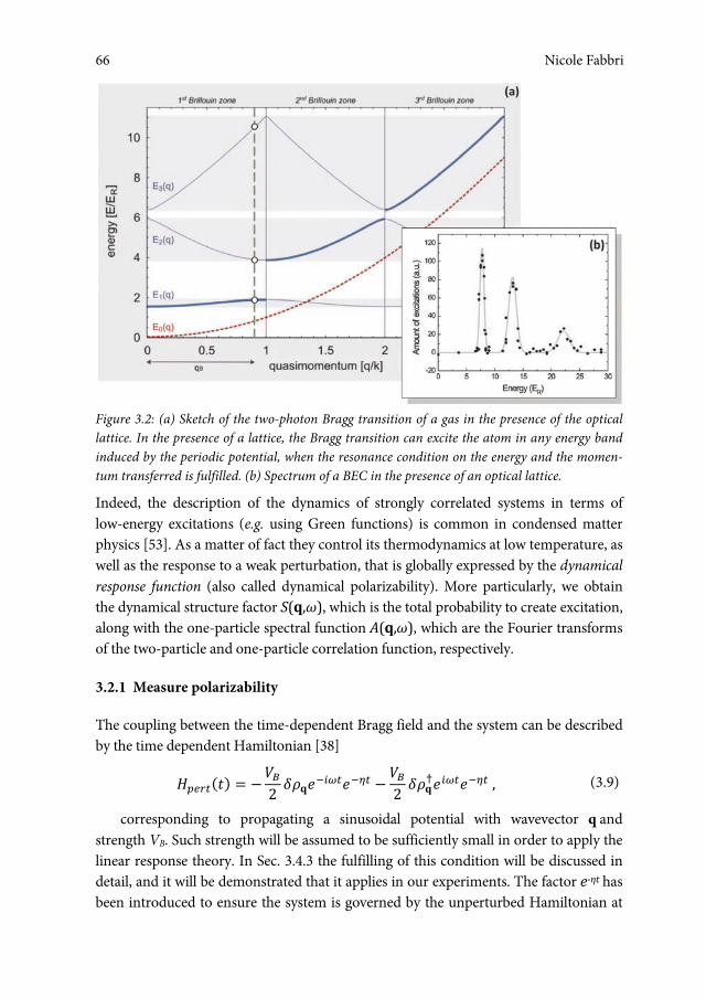
Nicole Fabbri
66
Figure 3.2: (a) Sketch of the two-photon Bragg transition of a gas in the presence of the optical lattice. In the presence of a lattice, the Bragg transition can excite the atom in any energy band induced by the periodic potential, when the resonance condition on the energy and the momen-tum transferred is fulfilled. (b) Spectrum of a BEC in the presence of an optical lattice.
Indeed, the description of the dynamics of strongly correlated systems in terms of low-energy excitations (e.g. using Green functions) is common in condensed matter physics [53]. As a matter of fact they control its thermodynamics at low temperature, as well as the response to a weak perturbation, that is globally expressed by the dynamical response function (also called dynamical polarizability). More particularly, we obtain the dynamical structure factor S(q,ω), which is the total probability to create excitation, along with the one-particle spectral function A(q,ω), which are the Fourier transforms of the two-particle and one-particle correlation function, respectively.
3.2.1 Measure polarizability
The coupling between the time-dependent Bragg field and the system can be described by the time dependent Hamiltonian [38]
�������� � ���2 ������������ � ��2 ������������ , (3.9)
corresponding to propagating a sinusoidal potential with wavevector q and strength VB. Such strength will be assumed to be sufficiently small in order to apply the linear response theory. In Sec. 3.4.3 the fulfilling of this condition will be discussed in detail, and it will be demonstrated that it applies in our experiments. The factor e‐ηt has been introduced to ensure the system is governed by the unperturbed Hamiltonian at
Nicole Fabbri66

Exploring the superfluid-to-insulator transition in a lattice
67
t = –. ��� � �� � ⟨��⟩ is the fluctuation of the q-component of the Fourier trans-form of the density operator ρ(x) = ψ†(x) ψ(x). The perturbation induces fluctuations of a certain physical observable ρq, which oscillates at the same frequency ω/(2π) as the external field. Precisely, polarizability provides the relationship of such fluctuations to the field, being defined as ⟨����⟩ � ����������� ���,ω� � ���������� ����,�ω�. (3.10)
Note that χ(q,ω) depends only on the properties of the system in the absence of any external perturbation.
Supposing that the system is in thermal equilibrium at temperature T at time t = –; it turns out [134]
���, �� � � 1����������
�,�� ⟨������⟩� � ��� � �� �
⟨�������⟩� � ��� � ��� (3.11)
where |n and |m are the eigenstates of the unperturbed Hamiltonian and ωn,m = (En ‐ Em)/� the transition frequencies between them. � � ∑ ������ is the partition function, with β = 1/(kBT). The Boltzmann factor ����� accounts for the thermal equilibrium of the initial configuration.
Polarizability is a complex function; thus it can be naturally separated into its real and imaginary parts ���,�� � ����,�� � � �����,�� (3.12)
where the real part χ’(q,ω) accounts for dispersion, whereas the imaginary part χ’’(q,ω) describes absorption properties (therefore, in the following it will be also referred to as the ‘dissipative component’ of the polarizability). Usually, experiments give access either to dispersive or dissipative components of the response function. For example in our case we measure the energy absorbed by the system, which is definitely easier to access than dispersion properties.10F10F10F
11 In the linear response theory, the energy absorbed by the system linearly depends
on the dissipative component of its dynamical polarizability χ’’(q,ω), as well as on the characteristics of the perturbing potential (amplitude VB and time duration ΔtB) [137], through the relation ��
�� �2�� ���2 �
�� �’’��, �� (3.13)
11 The whole response function can be reconstructed by exploiting the Kramers-Kronig relations [135, 136] that connect real and imaginary part of polarizability.
67Spectroscopy via inelastic light scattering

Nicole Fabbri
68
3.2.2 Low-energy excitations
The dynamical polarizability can be expressed in terms of the dynamical structure factor S(q,ω) [38], which is the Fourier transform of the two-particles correlation function.
S(q,ω) essentially describes the total probability to populate any excited state by transferring a momentum �q and energy �ω, provided that momentum and energy conservation can be met. Considering the zero-temperature case, initially the system can occupy only the ground-state |0 of the system with energy E0, and the dynamical structure factor reads
���, �� � 1�������
��⟨�� ����� � �������0⟩�� �
���� ���� � �� � ������(3.14)
where | ϕf and are possible final states of the system, with corresponding energies Ef. The operator ψ(q) creates a particle with momentum q. When Ef > E0 the system absorbs energy; in the opposite condition it releases energy. Since the initial state is the ground-state, only processes transferring energy to the system are allowed, since (Ef ‐ E0) is always positive.
Moreover, the dynamical structure factor obeys the relation ���,�� � �������,��� (3.15)
which expresses the detailed balancing which states that the probabilities to absorb or to release energy are related to each other by the Boltzmann factor ���. From Eq. (3.11) and (3.14) and the detailed balance relation (3.15), one can demonstrate that the dissipative component of polarizability is expressed in terms of S(q,ω) as �����,�� � � ����,��� � ���,���
� � �1 � �������, ��. (3.16)
Once the connection between the dissipative component of the response function and the dynamical structure factor has been ascertained, it is straightforward that the energy absorbed (the quantity measured in our experiments) is related to the dynamical structure factor. In fact, using the relation in Eq. (3.13), for a finite-time perturbation results in:
�� � 2�� ���2 �
�� ����,��� � ���,��� ���
� 2�� ���2 �
�� �1 � ���� ���, �����.
(3.17)
Nicole Fabbri68

Exploring the superfluid-to-insulator transition in a lattice
69
Figure 3.3: Dynamical structure factor S(q,ω) (green curve) and polarizability χ’’(q,ω) ∼ ωS(q,ω) (blue curve) of an array of 1D gases, both resulting from simulations at T = 100 nK (see Chapter 4 for a detailed explanation): The difference between the two functions is within the typical uncertainty in the experimental signal (vertical bar).
Thus, the energy absorption is sensitive to the difference [S(q,–ω) – S(q,ω)] rather than to the dynamic structure factor itself. This would be a difference between Bragg experiments and other scattering experiments, like neutron scattering from helium, where, by detecting the scattered probe, one instead measures directly the dynamic structure factor. Equation (3.17) says that the coupling with an external perturbation induces the system both to transfer and to release energy. Nevertheless, in general the dynamic structure factor exhibits a stronger dependence on temperature than χ’’(q,ω). For typical temperature of the system we investigate (T ∼ 100 ‐ 200 nK), the factor �1 � ���� which appears in Eq. (3.13) is negligible, so that it does not affect the response-signal significantly. Figure 1.3 compares χ(q,ω) and S(q,ω) simulated for an array of one-dimensional gases at temperature T = 100 nK (see Chapter 4): The difference is not significant compared to the typical uncertainty in the experimental signal, represented by a vertical bar.
3.2.3 Low-energy excitations in a lattice-gas
Up to now we have introduced general arguments to relate the energy absorbed by the system with the dynamical structure factor. This perfectly applies to the case of superfluid 1D gases. The situation is notably enriched when the 1D gas is immersed in a potential which varies periodically along the axis of the tube (longitudinal optical lattice): This has been the subject of the study that will be presented in Chapter 5 and 6.
69Spectroscopy via inelastic light scattering

Nicole Fabbri
70
Figure 3.4: (a) Excitation within the lowest-energy band (blue curve) of the system in a periodic potential, i.e., a particle-hole couple living in the ground state. (b) If the energy of the perturba-tion exceeds the band gap of the system, a particle is removed from the many-body ground-state, populating a single-particle state in a high-energy band and leaving a hole in the lowest band.
The simplest kinds of low-energy excited states involve either one or two qua-si-particles in the many-body ground-state and they are respectively connected to the one-particle spectral function A(q,ω) and the dynamical structure factor S(q,ω). As we will show later the inelastic scattering process we implement allows us to obtain information about these two quantities. Let us recall their meaning. S(q,ω) describes the probability of creating a particle-hole excitation with momentum �q and energy � within the many-body system. Its definition has been already introduced in Eq. (3.14). A(q,ω) essentially describes the probability of creating a hole in the ground-state by removing a particle with momentum �q and energy � and is de-fined as
���,�� � 1�������
��⟨�� |����|��⟩�� �
���� ���� � �� � ���� � ������(3.18)
where the same notation has been used as in Eq. (3.14). The operator ψ(q) creates a particle with momentum q. The energy ϵ(q) is that of the final excited state out of the many-body wave-function. Due to the presence of the periodic potential, the energy spectrum shows a band structure. In the following, the different bands will be labeled by the integer numbers n = 1, 2, …, ∞.
Since we realize 1D gases at ultra-low temperature, the atomic many-body state with N particles lies initially in the lowest-energy band (n = 1). As described in Sec. 3.1.2, in the presence of an optical lattice the two-photon Bragg transition can couple
Nicole Fabbri70
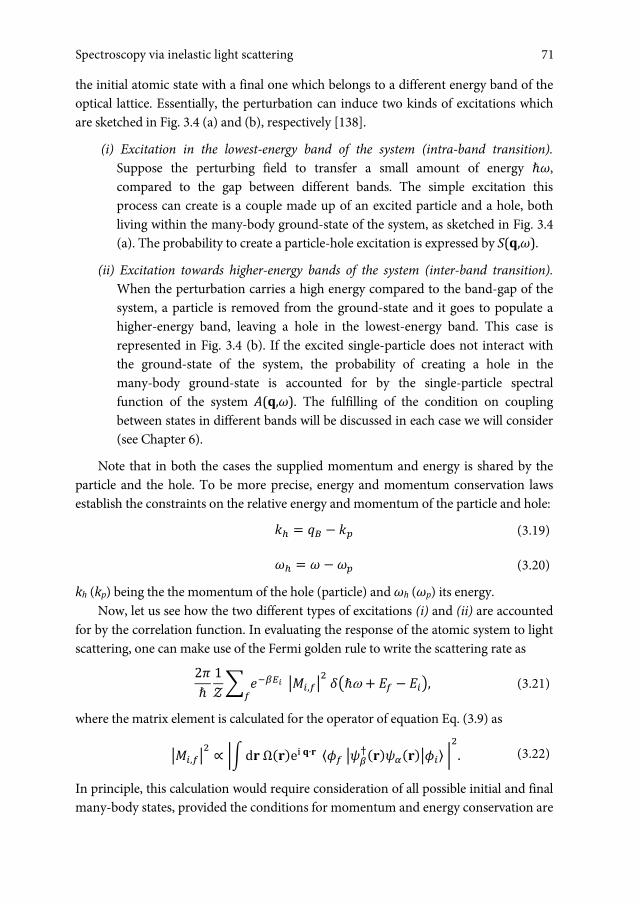
Exploring the superfluid-to-insulator transition in a lattice
71
the initial atomic state with a final one which belongs to a different energy band of the optical lattice. Essentially, the perturbation can induce two kinds of excitations which are sketched in Fig. 3.4 (a) and (b), respectively [138].
(i) Excitation in the lowest-energy band of the system (intra-band transition). Suppose the perturbing field to transfer a small amount of energy �ω, compared to the gap between different bands. The simple excitation this process can create is a couple made up of an excited particle and a hole, both living within the many-body ground-state of the system, as sketched in Fig. 3.4 (a). The probability to create a particle-hole excitation is expressed by S(q,ω).
(ii) Excitation towards higher-energy bands of the system (inter-band transition). When the perturbation carries a high energy compared to the band-gap of the system, a particle is removed from the ground-state and it goes to populate a higher-energy band, leaving a hole in the lowest-energy band. This case is represented in Fig. 3.4 (b). If the excited single-particle does not interact with the ground-state of the system, the probability of creating a hole in the many-body ground-state is accounted for by the single-particle spectral function of the system A(q,ω). The fulfilling of the condition on coupling between states in different bands will be discussed in each case we will consider (see Chapter 6).
Note that in both the cases the supplied momentum and energy is shared by the particle and the hole. To be more precise, energy and momentum conservation laws establish the constraints on the relative energy and momentum of the particle and hole:
�� � �� � �� (3.19)
�� � � � �� (3.20)
kh (kp) being the the momentum of the hole (particle) and ωh (ωp) its energy. Now, let us see how the two different types of excitations (i) and (ii) are accounted
for by the correlation function. In evaluating the response of the atomic system to light scattering, one can make use of the Fermi golden rule to write the scattering rate as ��
�1�� �����
����,��� ��� � �� � ���, (3.21)
where the matrix element is calculated for the operator of equation Eq. (3.9) as
���,��� � ���� ����e� ��� ⟨�� ���������������⟩ ��. (3.22)
In principle, this calculation would require consideration of all possible initial and final many-body states, provided the conditions for momentum and energy conservation are
71Spectroscopy via inelastic light scattering
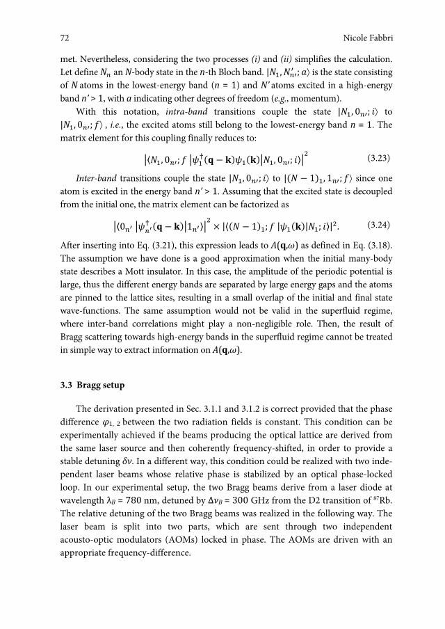
Nicole Fabbri
72
met. Nevertheless, considering the two processes (i) and (ii) simplifies the calculation. Let define �� an N-body state in the n-th Bloch band. |��, ���� � � is the state consisting of N atoms in the lowest-energy band (n = 1) and N’ atoms excited in a high-energy band n’ > 1, with a indicating other degrees of freedom (e.g., momentum).
With this notation, intra-band transitions couple the state |��, 0��� � to |��, 0��� � , i.e., the excited atoms still belong to the lowest-energy band n = 1. The matrix element for this coupling finally reduces to: �⟨��, 0��� � ������ � ����������, 0��� �⟩�� (3.23)
Inter-band transitions couple the state |��, 0��� � to |�� � 1��, 1��� � since one atom is excited in the energy band n’ > 1. Assuming that the excited state is decoupled from the initial one, the matrix element can be factorized as �⟨0�� ����� �� � ���1��⟩�� � |⟨�� � 1��� � |�����|��� �⟩|�. (3.24)
After inserting into Eq. (3.21), this expression leads to A(q,ω) as defined in Eq. (3.18). The assumption we have done is a good approximation when the initial many-body state describes a Mott insulator. In this case, the amplitude of the periodic potential is large, thus the different energy bands are separated by large energy gaps and the atoms are pinned to the lattice sites, resulting in a small overlap of the initial and final state wave-functions. The same assumption would not be valid in the superfluid regime, where inter-band correlations might play a non-negligible role. Then, the result of Bragg scattering towards high-energy bands in the superfluid regime cannot be treated in simple way to extract information on A(q,ω).
3.3 Bragg setup
The derivation presented in Sec. 3.1.1 and 3.1.2 is correct provided that the phase difference φ1, 2 between the two radiation fields is constant. This condition can be experimentally achieved if the beams producing the optical lattice are derived from the same laser source and then coherently frequency-shifted, in order to provide a stable detuning δν. In a different way, this condition could be realized with two inde-pendent laser beams whose relative phase is stabilized by an optical phase-locked loop. In our experimental setup, the two Bragg beams derive from a laser diode at wavelength λB = 780 nm, detuned by ΔνB = 300 GHz from the D2 transition of 87Rb. The relative detuning of the two Bragg beams was realized in the following way. The laser beam is split into two parts, which are sent through two independent acousto-optic modulators (AOMs) locked in phase. The AOMs are driven with an appropriate frequency-difference.
Nicole Fabbri72
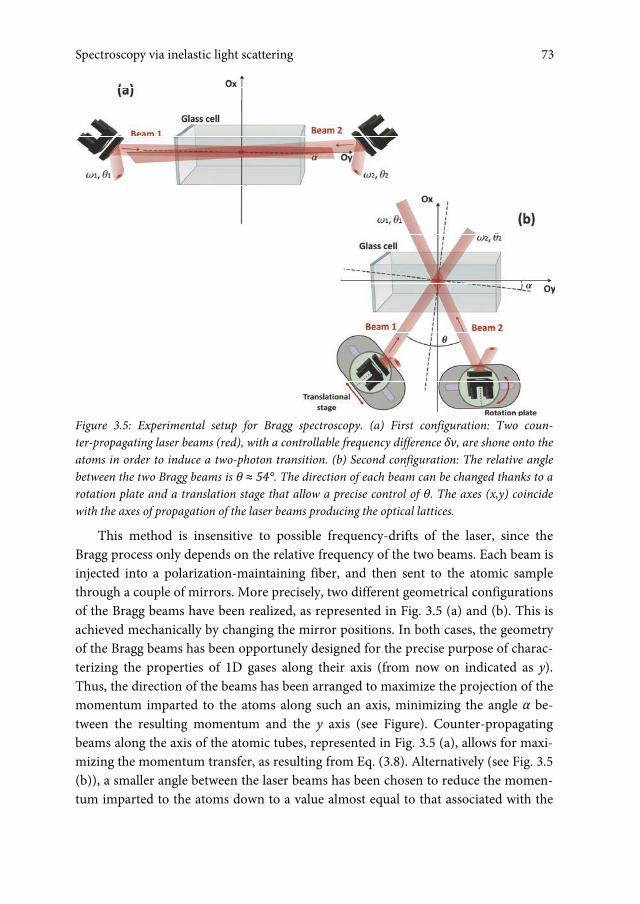
Exploring the superfluid-to-insulator transition in a lattice
73
Figure 3.5: Experimental setup for Bragg spectroscopy. (a) First configuration: Two coun-ter-propagating laser beams (red), with a controllable frequency difference δν, are shone onto the atoms in order to induce a two-photon transition. (b) Second configuration: The relative angle between the two Bragg beams is θ ≈ 54°. The direction of each beam can be changed thanks to a rotation plate and a translation stage that allow a precise control of θ. The axes (x,y) coincide with the axes of propagation of the laser beams producing the optical lattices.
This method is insensitive to possible frequency-drifts of the laser, since the Bragg process only depends on the relative frequency of the two beams. Each beam is injected into a polarization-maintaining fiber, and then sent to the atomic sample through a couple of mirrors. More precisely, two different geometrical configurations of the Bragg beams have been realized, as represented in Fig. 3.5 (a) and (b). This is achieved mechanically by changing the mirror positions. In both cases, the geometry of the Bragg beams has been opportunely designed for the precise purpose of charac-terizing the properties of 1D gases along their axis (from now on indicated as y). Thus, the direction of the beams has been arranged to maximize the projection of the momentum imparted to the atoms along such an axis, minimizing the angle α be-tween the resulting momentum and the y axis (see Figure). Counter-propagating beams along the axis of the atomic tubes, represented in Fig. 3.5 (a), allows for maxi-mizing the momentum transfer, as resulting from Eq. (3.8). Alternatively (see Fig. 3.5 (b)), a smaller angle between the laser beams has been chosen to reduce the momen-tum imparted to the atoms down to a value almost equal to that associated with the
73Spectroscopy via inelastic light scattering

Nicole Fabbri
74
lattice we use to realize and to drive atoms from a superfluid to a Mott-insulating state11F11F11F
12. While λB is precisely known in the experiment, the angle θ cannot be measured
geometrically with high precision. We use the atoms themselves as a sensor to precisely calibrate qB. For this purpose we measure the momentum transferred to a 3D BEC (in the absence of any optical lattice) in two different ways.
3.3.1 Calibration of the momentum transfer
Comparing spectra obtained by transferring two opposite momenta. In the first calibration measurement, we measure the resonant frequency of the Bragg spectrum for the 3D BEC. The resonance frequency depends on the momentum transfer hqB, on the strength of atom-atom interactions through the dispersion relation and on the initial velocity of the BEC center-of-mass. The dispersion relation E(q) of a trapped 3D BEC in the mean-field regime can be written as
���� � ���������� � ���2���, (3.25)
where cLDA(q) corresponds to an effective sound velocity within a local density approx-imation and is related to the mean-field interaction term [139]. The two-photon transi-tion induced by the Bragg pulse couples the initial state of the 3D BEC with momen-tum pi = �qi to an excited state with momentum pf = �(qi + qB). Thus the resonance energy of this process is E(qi + qB) – E(qi). In the absence of interactions, this energy reduces to the usual quadratic dependence of a single-particle spectrum
��.�.��� � ����� � ����2� � �����
2� . (3.26)
In order to reduce the effect on evaluating qB coming from interactions, we perform Bragg spectroscopy on dilute 3D BECs after a time-of-flight. When the magnetic trap is switched off, the BEC acquires a spurious nonzero momentum hqi. Thus, two unknown parameters have to be determined, qB and qi. We measure the spectra at positive (�qB) and negative (–�qB) momentum transfer.
The two resonance frequencies (E(qi + qB) – E(qi)) and qB allow us to precisely determine qB in the experiment. In the small-angle configuration, qB,y = 7.3(2) μm-1.
12 The response of a Mott insulator state has been predicted to be the strongest at the edge of the first Brillouin zone defined by the lattice which induces the transition [130].
Nicole Fabbri74

Exploring the superfluid-to-insulator transition in a lattice
75
In the experiment, the bisector of the two Bragg beams is not exactly perpendicular to the y-axis, and the momentum transferred along the y-axis is the projection
���,� � �� ��� ��� ��� ��2�
�� � ��|�� � ��| � ��, (3.27)
α being the small angle between the direction orthogonal to the beams bisector and the y-axis. To get an estimate of α, we diffract the atoms in the Raman-Nath regime [140] with very short light pulses (of typical duration 3 μs). In this regime, several orders of diffracted atoms are observed. This allows a good estimate of the axis along which the momentum is imparted by the light pulses to the atoms. Such a procedure has been used for both the lattice beams and the Bragg beams separately: The images of the atomic clouds diffracted by them are reported Fig. 3.6 (a), (b) and (c), respectively. From that, a relative angle between qB and the lattice has been measured, (see Fig. 3.6 (c)) obtaining α = 9.5(1)B. In conclusion, the projection of the momentum transfer along the y-axis indicates hqB,y= 0.96(3)hkL, where kL = 2/λL is the wavevector of the lattice beams at the wavelength λ = 830 nm. For the wavevector we obtain qB,y = 7.3(2) μm-1, which is indistinguishable from the modulus itself within the experimental uncertainty.
Figure 3.6: (a), (b), (c) Diffraction of a BEC by the lattice beams x and y and Bragg beams in Raman-Nath regime. The images in (a) and (b) depict the atoms in the plane (x-y), whereas (c) represents the plane (y-z). (d) Momentum imparted by Bragg beams qB (green arrow) compared to the direction of the wavevectors of the two lattices beam, indicated as x and y.
75Spectroscopy via inelastic light scattering

Nicole Fabbri
76
Bragg diffraction of a release BEC for different times-of-flight. In a second set of calibration measurements, we use the diffracted atoms of the 3D BEC by the moving lattice created with the Bragg beams. By letting the atoms fall under gravity after the Bragg pulse for a long enough time of flight (tTOF = 10 ‐ 30 ms), the diffracted atoms separate from the atoms which have not undergone the two-photon transition. The dis-tance between the two clouds is hqB,y tTOF/m in the (y-z) plane where absorption images are taken, m being the atomic mass. By fitting the distance between the diffracted and non-diffracted atomic clouds as a function of tTOF, we measure qB,y = 0.97(4) kL in good agreement with the previous measurement. In the configuration with coun-ter-propagating beams, an analogous estimate of the momentum imparted to the atoms gives qB = (16.04 " 0.15) μm-1.
3.3.2 Experimental procedure
The spectroscopic scheme described above has been used to probe the response of a correlated superfluid or insulating 1D Bose gases in the linear response regime, using the procedure depicted in Fig. 3.7 (a).
Figure 3.7: (a) Experimental protocol used to measure Δσ2, i.e., the increase of the squared-width of the central peak of the interference pattern after a Bragg pulse. Pictures (b) and (c) correspond to absorption images taken after an off-resonance and on-resonance Bragg pulse, respectively.
Nicole Fabbri76

Exploring the superfluid-to-insulator transition in a lattice
77
The atomic cloud is trapped in the lattice potential with amplitude s, sy by means of the exponential ramp described in Sec. 2.2.3. After a holding time of typically 20 ms in the lattices, it is excited by shining the two Bragg beams for a time ΔtB = 3 ms. In order to detect the amount of excitation induced by the Bragg beams in the correlated gaseous systems we follow a procedure similar to that used in [32] consisting in measuring a quantity related to the increase of energy in the gas, as we describe below.
Measuring the energy absorbed by the atoms. After the excitation, all the lattice amplitudes are linearly ramped down in 15ms to a low value (sy = s = 5), where the system is in a superfluid phase and the different tubes are no more independent, al-lowing the system to re-thermalize via atom-atom collisions. After 5 ms both optical and magnetic traps are simultaneously switched off abruptly and the system is ob-served via absorption imaging of the atomic distribution in the (y-z) plane after a time of flight (TOF) tTOF= 21 ms. Expanding from a phase coherent state in a 3D op-tical lattice (sy = s = 5), the atomic distribution exhibits an interference pattern which is the analogue of the diffraction pattern of light from a grating (see Fig. 3.8 (b) and [141, 142]).
Figure 3.8: (a) Experimental sequence used to measure the increase of temperature ΔT after a Bragg pulse and a thermalization time of 1 s in a 3D harmonic trap. Pictures (b) and (c) depict absorption images taken after an off-resonance and on-resonance Bragg pulse, respectively.
77Spectroscopy via inelastic light scattering

Nicole Fabbri
78
From this interference pattern we extract the root-mean-squared value of the widths σy and σz of the central peak. The increases of the quantity σ2 = σy2 + σz2 (from now on, it will be defined as Δσ2) is related to that of the energy of the system. Let us notice that we found σy and σz to have the same dependence on the detuning Δ between the Bragg beams as expected from an efficient rethermalization process in each spatial direction when the lattices are ramped down. The relation between Δσ2 and the energy growth is easy to demonstrate for a thermal gas with classical Maxwell-Boltzmann ve-locity distribution, where the squared size of the gas after time-of-flight is directly pro-portional to the temperature. In our case, we have verified this relation in practice, as we will describe in the next section.
3.4 Probe the excitations of the system
3.4.1 How to relate the experimental observable to the energy absorption
Now, we want to verify the quantitative relation between the quantity measured in the experiment, denoted Δσ2, and the energy absorbed by the gas. For this aim, we directly compare Δσ2 after a resonant Bragg excitation with the temperature increase ΔT induced under the same conditions (for identical Bragg excitation).
This comparison has been carried out for an array of 1D gases in a Mott insulating state, realized using a transverse optical lattice with amplitude s = 35 and a longitudinal lattice at sy = 13 (see Chapter 6); excitation in the second band of the lattice has been considered in this test, by selecting the appropriate relative detuning between the Bragg beams. The temperature of the system after Bragg excitation is measured by ramping down adiabatically the optical lattices with an exponential ramp after the Bragg pulse, letting the system thermalize in the harmonic magnetic trap for 1 s and then measuring the condensate fraction of the 3D atomic cloud. The experimental protocol is illustrated in Figure 3.8 (a). Figure 3.8 (b) and (c) report two absorption images taken after off-resonance and on-resonance Bragg excitation. In the first case the profile of the gas is well described by an inverted parabola, the signature of an almost-pure condensate in the Thomas-Fermi regime. After on-resonance excitation, a bimodal density profile is visible, where a gaussian pedestal can be recognized below the inverted parabola, revealing that the condensed fraction is sensibly decreased. By changing the power in the Bragg beams, Δσ2 is tuned over the whole range typically used in experiments. The results are presented in Figure 3.9 where ΔT has been extracted from the decrease of the condensate fraction. This measurement confirms that Δσ2 is proportional to the energy absorbed by the atomic system, i.e., to the number of excitations created.
Nicole Fabbri78

Exploring the superfluid-to-insulator transition in a lattice
79
Figure 3.9: Linear behaviour of Δσ2 as a function of the increase of temperature ΔT of an array of 1D gases in the Mott insulator regime (sy = 13, s = 35) perturbed via Bragg scattering. Data points correspond to different power of the Bragg beams with a fixed pulse length of 3 ms.
In addition to what we demonstrated above, it is possible to verify that the amount of excitation we measure by means of Δσ2 is ωS(q,ω), definitely distinguishing it from S(q,ω). As a testing ground, we use an array of gases in deep 1D conditions (s = 45). To achieve our purpose, we check the relation between Δσ2 and ΔT for two different values of relative detuning δν1 and δν2 between the Bragg beams, namely for two dif-ferent frequencies of the excitation created in the gas. These values have been oppor-tunely chosen so that one is twice the other (δν1 = 3.2 kHz and δν2 = 6.4 kHz) and so that we observe the same amount of excitation for each, as shown in Fig. 3.10 (a). As observed above for a Mott insulating state, we find again a linear dependence of Δσ2 on ΔT for both values of detuning (Fig. 3.10 (b)). Moreover, from comparison of the two slopes, we extract additional information. If the amount of excitations were a meas-urement of S(q,ω), the ratio of the two slopes (i.e., the ratio of the amount of excitation to the temperature) would be the inverse of the ratio of the two frequencies, being S(q,ωi)/Ti – 1/ωi. On the contrary, the observed slope is independent of the excitation frequency: This demonstrates that we measure a quantity proportional to ωS(q,ω).
We conclude this Section with a final remark about the measurement technique here illustrated. One may wonder whether the spectra could be obtained by measuring the condensate fraction instead of Δσ2. This could be the case when the amplitude of the response of the 1D gases is large as in the superfluid regime or in a Mott regime for high-energy bands. In contrast, the amplitude of the response of the Mott insulating state within the lowest energy band is low as the system exhibits its insulating behavior.
79Spectroscopy via inelastic light scattering

Nicole Fabbri
80
Figure 3.10: (a) Bragg spectrum of an array of 1D gases (s = 45). (b) Amount of excitation as a function of increase of temperature induced by the Bragg excitation at two different frequencies ν1 (red squares) and ν2 (blue dots), indicated by markers in the spectrum (a).
In this case, the measurement of σ2 is definitely more sensitive than that of the condensate fraction, allowing the detection of even small excitations.
3.4.2 Amount of excitations �
In the last Section, it was demonstrated that the quantity defined as Δσ2 is directly proportional to the energy absorbed by the gas because of the Bragg excitation. Thus it is a relevant quantity, giving access either to the dynamical structure factor or to the one-particle spectral function, as described in Sec. 3.2.2.
Nicole Fabbri80
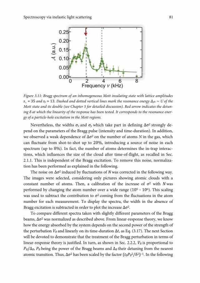
Exploring the superfluid-to-insulator transition in a lattice
81
Figure 3.11: Bragg spectrum of an inhomogeneous Mott insulating state with lattice amplitudes s = 35 and sy = 13. Dashed and dotted vertical lines mark the resonance energy Δph ∼ U of the Mott state and its double (see Chapter 5 for detailed discussion). Red arrow indicates the detun-ing δ at which the linearity of the response has been tested. It corresponds to the resonance ener-gy of a particle-hole excitation in the Mott regions.
Nevertheless, the widths σx and σy which take part in defining Δσ2 strongly de-pend on the parameters of the Bragg pulse (intensity and time-duration). In addition, we observed a weak dependence of Δσ2 on the number of atoms N in the gas, which can fluctuate from shot-to-shot up to 20%, introducing a source of noise in each spectrum (up to 8%). In fact, the number of atoms determines the in-trap interac-tions, which influences the size of the cloud after time-of-flight, as recalled in Sec. 2.1.1. This is independent of the Bragg excitation. To remove this noise, normaliza-tion has been performed as explained in the following.
The noise on Δσ2 induced by fluctuations of N was corrected in the following way. The images were selected, considering only pictures showing atomic clouds with a constant number of atoms. Then, a calibration of the increase of σ2 with N was performed by changing the atom number over a wide range (105 ‐ 106). This scaling was used to subtract the contribution to σ2 coming from the fluctuations in the atom number for each measurement. To display the spectra, the width in the absence of Bragg excitation is subtracted in order to plot the increase Δσ2.
To compare different spectra taken with slightly different parameters of the Bragg beams, Δσ2 was normalized as described above. From linear-response theory, we know how the energy absorbed by the system depends on the second power of the strength of the perturbation VB and linearly on its time-duration Δt, as Eq. (3.17). The next Section will be devoted to demonstrate that the treatment of the Bragg perturbation in terms of linear-response theory is justified. In turn, as shown in Sec. 2.2.2, VB is proportional to PB/ΔB, PB being the power of the Bragg beams and ΔB their detuning from the nearest atomic transition. Thus, Δσ2 has been scaled by the factor (tBPB2/δ2)–1. In the following
81Spectroscopy via inelastic light scattering

Nicole Fabbri
82
we will refer to the re-normalized Δσ2, called �, as the amount of excitation transferred to the system. The plot of � as a function of the detuning δ between the two Bragg beams gives the excitation spectrum. In Fig. 3.11 we show an example of a spectrum of the inhomogeneous Mott insulating state (see Chapter 5 and [50]).
3.4.3 Linear response
The linearity of the response of the system to the Bragg excitation has been studied by monitoring how Δσ2 varies with the parameters of the Bragg excitation on reso-nance. The frequency of the Bragg excitation was fixed at ω = 2πΔph/h (red arrow on Fig. 3.11), i.e., on the main resonant peak of the Mott insulating state, which we identify as the frequency of the particle-hole excitation in the lowest band Δph [50](see Chapter 5). Δσ2 was measured as a function of the amplitude VB of the Bragg lattice and the du-ration ΔtB of the pulse, with the results plotted on Fig. 3.12. In the range of parameters used to monitor the spectra12F12F12F
13, Δσ2 shows a quadratic dependence on VB and a linear dependence on ΔtB, according to that predicted by linear-response theory. The inset of Fig. 3.12 (b) compares the variation of Δσ2 as a function of the pulse duration ΔtB for two amplitudes VB, namely VB = 0.5ER (dots) and VB = 2.0ER (circles) at ω = 2πΔph/h for sy = 13. For the larger amplitude VB = 2.0 ER the response to the Bragg excitation exhibits a saturation and the time scale of the linear regime is short-er. We note that we did not observe Rabi oscillations as in the case of excitation from the ground-state of a 3D BEC in a harmonic trap and a Bogoliubov mode [122]. In the latter case the excited state is decoupled from the ground-state, a situation which might not be true anymore in the Mott state where strong correlations are present.
In addition, the amplitude VB of the moving lattice created by the Bragg beams for such parameters is much smaller than the amplitude of the longitudinal lattice sy used to realize the Mott insulating phase. All the experiments are performed in a regime where VB < 0.05 Vy. This regime is different from the one where the Bragg spectrum of a Mott insulator has been obtained in previous experiments [32, 35] using the lattice modulation technique. In the latter case, the amplitude of the lattice has been typically modulated by ∼ 30%, because the measurements are performed at zero momentum transfer, where the response of the Mott insulator is predicted to be weak [130]. In con-trast, in the present work the parameters U and Jy describing the system in the Bose-Hubbard model (see Sec. 1.4.1) are almost unaltered by the additional light poten-tial created by the Bragg beams.
13 For instance, the spectrum at sy =13 in Fig. 3.11 has been obtained with VB = 0.5 ER and ΔtB = 6 ms.
Nicole Fabbri82

Exploring the superfluid-to-insulator transition in a lattice
83
Figure 3.12: (a) Δσ2 as a function of the amplitude VB of the lattice induced by the Bragg beams, which is proportional to the power PB. The measurement is performed at a fixed energy transfer ω = 2πΔph/h corresponding to the resonance of the particle-hole excitation and for a duration of the Bragg pulse ΔtB = 3 ms. Inset: The same measurement on a larger scale of the amplitude VB showing saturation for VB > ER. (b) Δσ2 as a function of the duration of the Bragg pulse at a given amplitude VB = 0.5 ER. As in (a), the measurement is performed at the energy ν = Δph/h of the particle-hole excitation. Inset: Comparison of the response for two amplitudes VB, namely VB = 0.5 ER (dots) and VB = 2.0 ER (circles).
Δσ2 also saturates for large amplitudes VB as depicted in the inset of Fig. 3.12(a). In addition, the amplitude VB of the moving lattice created by the Bragg beams for
such parameters is much smaller than the amplitude of the longitudinal lattice sy used to realize the Mott insulating phase. All the experiments are performed in a regime where VB < 0.05 Vy. This regime is different from the one where the Bragg spectrum of a Mott insulator has been obtained in previous experiments [32, 35] using the lattice modulation technique. In the latter case, the amplitude of the lattice has been typically modulated by ∼ 30%, because the measurements are performed at zero momentum transfer, where the response of the Mott insulator is predicted to be weak [130]. In con-trast, in the present work the parameters U and Jy describing the system in the Bose-Hubbard model (see Sec. 1.4.1) are almost unaltered by the additional light poten-tial created by the Bragg beams.
3.4 Conclusions
The discussion presented in this Chapter has shown that the probe technique used in the work of this thesis, namely Bragg scattering, can be used as a powerful and versa-tile spectroscopic method; it allows the characterization of condensed-matter physics systems as well as strongly-correlated phases realized with ultracold gases. Not only
83Spectroscopy via inelastic light scattering

Nicole Fabbri
84
does it allow independent tuning of the energy and momentum of the excitation in-duced in the system, offering the possibility of completely scanning the whole excita-tion spectrum of the system, but also it weakly perturbs the state of the system under investigation. With appropriate choice of parameters, the amount of excitation in-duced in the system varies linearly with the parameters of the probe: This has been proven to apply in our experiment. This is a crucial point, since for this condition the process is well described by linear-response theory. Thus, the Bragg spectra we meas-ure are directly related to the correlation functions of the system, the knowledge of which highlights the physics governing the system. In particular, we demonstrated that the spectra measured for a correlated superfluid and a Mott insulator in the low-est energy band are proportional to the dynamical structure factor S(q,ω) [143], whereas the excitation-spectra of a Mott insulator state in the high-energy bands give information on the one-particle spectral function A(q,ω).
In the next Chapters (4, 5 and 6) we will pursue our aim to characterize such strongly-correlated quantum phases realized by one-dimensional atomic micro-gases, exploiting Bragg spectroscopy.
Nicole Fabbri84

Chapter 4 Thermal phase-fluctuations in one dimension
The knowledge of quantum and thermal fluctuations, strongly enhanced by reduced dimensionality, gives access to key quantities characterizing the system [56]. In one dimension, their presence can drastically alter the properties of the systems. Remark-able examples of that are superconducting disordered nanowires, where quantum and thermal fluctuations can lead to the formation of phase-slip centers [144, 145], which strongly affect the resistivity of such materials.
In this Chapter, we report on the investigation of the coherence properties of an array of one-dimensional Bose gases with short-scale phase fluctuations. The momentum distribution is measured using Bragg spectroscopy and an effective coherence-length of the whole ensemble is defined. In addition, we propose and demonstrate that time-of-flight absorption imaging can be used as a simple probe to directly measure the coherence-length of 1D gases in the regime where phase-fluctuations are strong. This method is suitable for future studies such as for investigating the effect of disorder on the phase coherence. We also develop a simulation of the response of our inhomogeneous array, as a sum of the contributions of all the 1D gases, due to interactions and fluctuations. Finally, we extract an estimate of the temperature of the system.
4.1 Introduction
In the context of cold atoms, both phase and density fluctuations of 1D systems have been studied during the last few years [103, 106, 108, 107]. In particular, phase coher-ence has been investigated in elongated 3D quasicondensates with different tech-niques [103, 106, 107]. In the experiment of S. Hofferberth et al. [103] phase dynam-ics has been followed by monitoring interference between two different 1D gases. S. Dettmer et al. [106] observed density-modulations of the atomic cloud released from the trap, which results from phase-modulation of the trapped sample. Such work points out the statistical character of phase-fluctuations. In the experiment by S. Richard et al. [107], phase coherence was also investigated by means of the response
Nicole Fabbri, Bragg spectroscopy of quantum gases: Exploring physics in one dimension isBN 978-88-6655-220-8 (print) isBN 978-88-6655-221-5 (online) © 2012 Firenze University Press

Nicole Fabbri
86
to light scattering, by measuring coherence lengths of the order of 10 μm. Neverthe-less, in all of these realizations the transverse trapping frequencies hardly exceed a few kHz and are typically of the order of the chemical potential. This situation is re-ferred to as the quasi-1D regime.
Reaching the regime of strongly interacting 1D systems would further amplify the presence of quantum and thermal fluctuations. This is achieved when atoms are loaded in a 2D optical lattice allowing much stronger transverse confinements [33, 34, 104]. Following this approach, we realize an array of strongly phase-fluctuating 1D Bose gases, represented in Fig. 4.1 (a). Each 1D gas in the array is a quasicondensate, where density fluctuations are suppressed (Fig. 4.1 (b)), whereas longitudinal phase fluctuations are present and enhanced due to the anisotropy of our system (Fig. 4.1 (c)). Yet, making use of optical lattices one obtains a large number of 1D tubes. In this case, interferometry-based techniques like in [103, 106] cannot be implemented to study the phase coherence properties since the average over different gases washes out the response signal and it is particularly important to find alternative methods to analyze the axial coherence properties.
Figure 4.1 (a) Schematic view of the two-dimensional array of one-dimensional gases. (b) Densi-ty profile along the axial direction. (c) Example of phase profile along the same axial direction showing fluctuations on a length scale much smaller than the axial size.
Nicole Fabbri86

Exploring the superfluid-to-insulator transition in a lattice
87
Our study exploits first Bragg spectroscopy with large momentum-transfer to measure the momentum distribution and directly evaluate the ‘radius’ of the phase fluctuations Lϕ, that is, the mean distance along which the phase of the system varies by 2π [107]. In our case, thermal-induced phase-fluctuations dominate and drastically reduce the coherence length (2Lϕ) of the system compared to a 3D Bose-Einstein condensate [62, 54]. In addition, we verify that direct mapping of the momentum distribution onto coordinate space via absorption imaging after TOF is an effective probe of the phase fluctuations. We demonstrate that in our regime of parameters these two techniques give the same results.
4.1.1 The experiment
The system under study consists of an array of 1D gases of 87Rb. The gases are trapped in a slow-varying magnetic trap and forced in the 1D geometry by a pair of orthogonal red-detuned optical lattices aligned along the x and z directions. We study different configurations starting from a 3D gas and dividing it into 1D micro-tubes that are more and more squeezed. This is obtained by tuning the amplitude s of the 2D optical lattice.
Increasing the amplitude of the 2D lattice from s = 5 to s = 56, the frequency of on-site transverse confinement of each 1D gas changes from ∼ 2π × 15 kHz to ∼ 2π × 50 kHz. Also, the axial confinement given by the Gaussian profile of the beams producing the lattices becomes stronger as s grows, being ωy ∼ 2π × 19 Hz for s = 5 and ωy ∼ 2π × 57 Hz for for s = 56. Globally, the stronger the optical confinement, the more anisotropic is the trap experienced by each 1D gas: The aspect ratio λ = /ωy ranges from 790 to 880 for 5 < s < 56. As discussed in Sec. 2.3, for all the amplitudes of the transverse lattice we have explored (s ≥ 5) each gas has a fully 1D character, i.e. both the chemical potential and the thermal energy are about one order of magnitude smaller than the frequency of the transverse harmonic oscillator (typically, in the most unfavorable case of s = 5 the thermal population of the first transverse excited-state amounts to about 0.1% of the ground-state).
Exploiting the model we developed in Sec. 2.3, it is possible to calculate the main features of the array, which change as the transverse confinement is modified. For s = 5 the array consists of ∼ 800 micro-tubes, with typical total size 0.08 μm × 50 μm and density 6 μm-1. For the most confining lattice that we realize, s = 56, we produce ∼ 1.8 × 10³ 1D gases, with total size ∼ 0.05 μm × 30 μm and density ∼ 5 μm-1. For the transverse size of each gas, we have to consider the amplitude of the transverse zero point oscillations in the lattice sites, whereas along the axial direction we have taken the Thomas-Fermi radius, having demonstrated in Sec. 2.3.1 the longitudinal profile to be parabolic. Besides, due to the inhomogeneity of the array, we have considered an average value of the 1D density of the gases (weighted with the number of atoms of
87Thermal phase-fluctuations in one dimension

Nicole Fabbri
88
each tube). We note that the modification of the transverse confinement hardly affects such a 1D density.
As mentioned in Sec. 1.3.1, a crucial quantity to describe the regime of a 1D gas is the parameter γ = mg1D��2 ρ0. In the system we realize, γ ∼ 0.2 – 0.8, i.e., the universal parameter K is larger than 3, according to Eq. (1.9). Therefore interparticle correlations are stronger than in the mean-field regime (as in other experiments probing a similar range of parameters, see for example [104]).
Figure 4.2: Schematic phase diagram for a 1D gas trapped with α ≃ 6.6, represented in the plane of temperature (rescaled with the longitudinal trapping frequency) and number of atoms (which is simply related to the density for a system with finite size). The figure is adapted from [54], by rescaling the vertical axis. A dilute gas at high temperature is a classical gas (right-hand side of the diagram, on the bottom). On the other hand, a cool and dense sample experience the regime of Bose-Eintein condensate, where all the particles behave as a unique object, with spatial long-range coherence overall the system (without density fluctuations in space) and described by a global wavefunction with a defined phase. For intermediate values of temperature and density, the system enters a regime where density fluctuations are suppressed whereas the phase of the wavefuntion still suffers fluctuations, so-called quasi-condensate regime. Finally, at sufficiently low temperature, diminishing density induces interation energy to dominate over kinetic energy, up to reach the fermionized Tonks-Girardeau regime. The red vertical strip represents our sys-tem, for typical temperatures achieved in the experiment.
Another relevant quantity for describing the system is the parameter α = mg1Day��2 introduced in Sec. 1.3.2. Through the dependence on the axial harmonic-oscillator length ay and on the 1D coupling constant g1D (see Eq. (2.30)), α only depends on the axial trapping frequency and on the lattice depth, apart from the characteristics of the atomic species itself (mass and 3D scattering length), whereas it is
Nicole Fabbri88

Exploring the superfluid-to-insulator transition in a lattice
89
independent from the 1D density. Thus, α assumes the same value over the entire array, no matter if inhomogeneous. In this experiment, α = 3.6 – 7.6 for s = 5 – 56.
For a fixed lattice depth, a knowledge of α allows us to locate the state of the system in a phase diagram in the N–T plane [54], N being the number of atoms in the single 1D gas and T its temperature. In Fig. 4.2 we report such a phase diagram for s = 35, corre-sponding to α = 6.6: It has been adapted from [54], simply by rescaling the number of atoms of the 1D gas by a factor 0.66. For such a value of the lattice depth, we expect the temperature to be ∼ 100 nK (see Sec. 4.5) and the axial frequency ωy ∼ 45 Hz, which results in kBT���ωy) ∼ 40. Because of the inhomogeneity of the array, an extended range of N is realized, represented by a red band in the diagram13F,13F13F
14 the upper border of which represents the 1D gas in the central lattice-site, having the largest number of at-oms. As depicted in the figure, the inner gases are in a quasicondensate phase. Moving from the center of the trap, the atom number decreases: Below the critical value N* ≡ α2 ∼ 40, realized at a sufficiently large distance from the center of the trap, the gases should enter the Tonks-Girardeau regime (light-blue region below the dashed line in the figure). In the outermost region of the lattice we expect the 1D-density to be so low that the gas lies in the classical regime, where no phase coherence exists. These low-density gases are numerous, as the number of tubes scales with the squared dis-tance from the center of the trap. Yet, the response of each gas contributes to the global signal proportionally to its atom number, as we will show in Sec. 4.4. Therefore, we ex-pect the response of the inner gases to dominate, even though they are less numerous: This is indicated by colour saturation of the red rectangle in the figure.
4.2 Investigate coherence properties via Bragg scattering The effect of the phase-fluctuations is first investigated via Bragg spectroscopy. In this experiment, two series of measurements have been performed, using the two different geometrical configurations of the Bragg beams we described in Sec. 3.3, imparting a momentum �qB, 1= ��16.0�2) μm-1 and �qB, 2= ��7.3�2) μm-1 respectively. In both cases, the geometry of the Bragg beams is chosen so that �qB is aligned along the axis of the 1D tubes). For both the Bragg configurations that we use, we assume to be in the large momentum-transfer regime (Doppler regime) [139], where the reference momentum is qξ = ξ ‐1, � � ���� �������� being the healing length of the system. The typical chemical potential ������ of the system ranges from 1 kHz to 3 kHz, so that for
14 The width of this band describes the uncertainty of the estimated temperature (∼ 90 nK) at s = 35. For a discussion about temperature, see Sec. 4.5.
89Thermal phase-fluctuations in one dimension

Nicole Fabbri
90
the case of counter-propagating beams qB/qξ ranges from 3.2 to 5.5, whereas for the small-angle configuration from 1.4 to 2.5.
Figure 4.3: Excitation spectra of arrays of strongly correlated 1D gases trapped in optical lattices with different amplitudes s. The spectra are obtained with momentum transfer �qB,2 = �×���(2) μm-1. Blue curves are the results of a fitting procedure of the function ν × f(ν), where f(ν) is a Lorentzian function.
Nicole Fabbri90

Exploring the superfluid-to-insulator transition in a lattice
91
The procedure described in Sec. 3.3.2 allows us to measure the energy transferred to the system, which is related to the dynamical structure factor of the system through χF”(ω) = π S(q, ω) (1 – e –�ω/(kBT)) as discussed in Sec. 3.2. In the Doppler regime, S(q, ω) reduces directly to the momentum distribution ����� [121, 107], which can be written as the Fourier transform of the first-order correlation function �������:
����� � 12�� ��� ������������ (4.1)
The spectra resulting from these measurements for a transferred momentum �qB, 2 are reported in Fig. 4.3.
Central frequency of the resonances. In the Doppler regime, assuming a mean-field picture to treat the interactions14F14F14F
15, the spectrum assumes a single-particle-like form with an additional mean-field shift
���� � ����2� � ���� (4.2)
���� being the chemical potential of a 1D gas. Thus, energy and momentum conserva-tion for the two-photon Bragg transition implies that the energy hv transferred to the system to be
�� � ��� � ���� � ������� (4.3)
where �qi is the momentum of the initial state and �ωB the energy of the Bragg excita-tion. Starting from a gas at rest (qi = 0), the central frequency νc of the energy spectrum is expected to be given simply by �� � ��/�2�� � ����/� . Actually, the inhomogene-ous density of each trapped 1D quasicondensate along its axial direction modifies this mean-field shift to �����/� [121]. As discussed in Sec. 2.3.2, the chemical potential monotonically increases as a function of the amplitude of the transverse confinement s, and thus we expect the mean-field shift to grow consequently.
Fig. 4.4 reports the central frequency of the observed resonances as a function of the amplitude s of the lattices, at fixed wavevector of the excitation qB,2. The gray dashed line represents the single-particle energy �ωB, whose uncertainty covers the entire region between the gray solid lines. As expected, the resonance centers drift toward higher frequencies as the lattice amplitude increases, due to the enhanced interactions, qualitatively confirming the picture we described above.
15 For the values of γ we realize in the experiment, the resonant frequencies of the Lieb-Liniger modes are expected to be indistinguishable from the mean-field solution within our experimental resolution [146].
91Thermal phase-fluctuations in one dimension
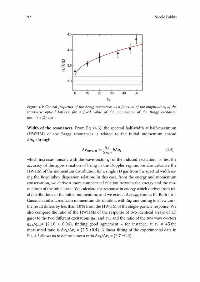
Nicole Fabbri
92
Figure 4.4: Central frequency of the Bragg resonances as a function of the amplitude s of the transverse optical lattices, for a fixed value of the momentum of the Bragg excitation qB,2 = 7.3(2) μm-1.
Width of the resonances. From Eq. (4.3), the spectral half-width at half-maximum (HWHM) of the Bragg resonances is related to the initial momentum spread �Δqi through Δ����� � ��
2����� (4.4)
which increases linearly with the wave-vector qB of the induced excitation. To test the accuracy of the approximation of being in the Doppler regime, we also calculate the HWHM of the momentum distribution for a single 1D gas from the spectral width us-ing the Bogoliubov dispersion relation. In this case, from the energy and momentum conservation, we derive a more complicated relation between the energy and the mo-mentum of the initial state. We calculate the response in energy which derives from tri-al distributions of the initial momentum, and we extract ΔνHWHM from a fit. Both for a Gaussian and a Lorentzian momentum distribution, with Δqi amounting to a few μm-1, the result differs by less than 10% from the HWHM of the single-particle response. We also compare the ratio of the HWHMs of the response of two identical arrays of 1D gases to the two different excitations qB,1 and qB,2 and the ratio of the two wave-vectors qB,1/qB,2= (2.16 ± 0.06), finding good agreement – for instance, at s = 45 the meausured ratio is Δν1/Δν2 = (2.5 ±0.4). A linear fitting of the experimental data in Fig. 4.5 allows us to define a mean ratio Δν1/Δν2 = (2.7 ±0.8).
Nicole Fabbri92
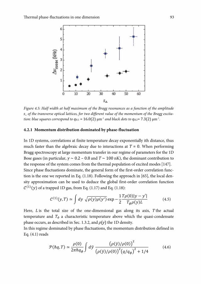
Exploring the superfluid-to-insulator transition in a lattice
93
Figure 4.5: Half width at half maximum of the Bragg resonances as a function of the amplitude s of the transverse optical lattices, for two different value of the momentum of the Bragg excita-tion: blue squares correspond to qB,1 = 16.0(2) μm-1 and black dots to qB,2= 7.3(2) μm-1.
4.2.1 Momentum distribution dominated by phase-fluctuation
In 1D systems, correlations at finite temperature decay exponentially ith distance, thus much faster than the algebraic decay due to interactions at T = 0. When performing Bragg spectroscopy at large momentum transfer in our regime of parameters for the 1D Bose gases (in particular, γ ∼ 0.2 – 0.8 and T ∼ 100 nK), the dominant contribution to the response of the system comes from the thermal population of excited modes [147]. Since phase fluctuations dominate, the general form of the first-order correlation func-tion is the one we reported in Eq. (1.18). Following the approach in [65], the local den-sity approximation can be used to deduce the global first-order correlation function ������� of a trapped 1D gas, from Eq. (1.17) and Eq. (1.18):
������, �� ≃ ��� ���������� ����12���0�|� � ��|������� (4.5)
Here, L is the total size of the one-dimensional gas along its axis, T the actual temperature and Tϕ a characteristic temperature above which the quasi-condensate phase occurs, as described in Sec. 1.3.2, and ρ(y) the 1D density. In this regime dominated by phase fluctuations, the momentum distribution defined in Eq. (4.1) reads
����, �� ≃ ��0�2���� ���� ���������0���
���������0���������� � 1�� (4.6)
93Thermal phase-fluctuations in one dimension

Nicole Fabbri
94
where �� � �� � ���/�, and we approximated ���������� � �����. The momentum distribution is self-similar in qy/qϕ, and is well approximated by a normalized Lorentzian. Its half width at half maximum ��qy depends only on the coherence length of the gas, being [148]
�� � 0.635�� (4.7)
where Lϕ is the half coherence length, i.e., the radius of phase fluctuations:
�� � ������� (4.8)
Thus, for an axially trapped 1D gas dominated by phase fluctuations, one finds again the Lorentzian momentum distribution of a uniform 1D gas [62, 54], with only a correction to the factor 0.635 in the HWHM, which takes into account the parabolic profile of the system along the axial direction as well as the 1D character (for a 3D Thomas-Fermi profile one obtains a factor 0.67 [65]). Therefore, in the following, we will focus on the width of the energy spectra observed in the experiment, which carry information on the coherence of the system.
4.2.1 Effective coherence length
In our case the description of the problem is complicated by the presence of an in-homogeneous array made up of gases with different densities (thus, different charac-teristic Lϕ). In principle, one should take into account the sum of the response of each micro-tube, which is affected by interactions and phase fluctuations. Both the mean-field shift of the central frequency and the thermal broadening of the width depend on the 1D density, which is not uniform over the array.
Nevertheless, we observe that the global response of the system to the Bragg excitations consists of a single broad resonance, as shown by the spectra in Fig. 4.3. In the range of parameters we realize, the shape of the resonance is well described by ν × f(ν) ≃ ωS(q,ω) where f(ν) is a Lorentzian function. This means that, in our case, the thermal broadening of the response of each gas masks the relative shifts of the resonant frequencies of the tubes. This has been also verified a posteriori by means of numerical simulations we will present in Sec. 4.4. On the basis of these arguments, we analyze the Bragg spectra as being the response of a single 1D gas and we define accordingly an effective coherence-length Lϕ of the whole system, using the previous relations valid in the Doppler regime. This would be the coherence length of an array of identical 1D gases with the same effective density, whose response would reproduce that of the inhomogeneous array.
Nicole Fabbri94

Exploring the superfluid-to-insulator transition in a lattice
95
From the fittings of the Bragg spectra, we extract the HWHM Δν. This quantity is reported in Fig. 4.5 as a function of the amplitude s of the optical lattices and for two different wave-vectors of the excitation qB,1, qB,2 (blue squares and black dots). The total number of atoms is kept almost constant in both series of data. From the spectral half-width of the Bragg spectra, we extract the half-length Lϕ. As shown in Fig. 4.6, Lϕ drops off by a factor 5 as s increases from 5 to 56. We note that for higher s values the coherence length becomes comparable to the inter-particle distance. In addition, the analysis of the Bragg spectra for the two momentum transfer qB,1 and qB,2 gives identical Lϕ as expected in the Doppler regime. From Eq. (4.8), Lϕ depends both on the 1D density ρ and on the temperature T. The optical confinement makes the aspect ratio of the 1D gases grow and their density decrease. However, as mentioned before, on the basis of our theoretical model, we estimate that the relative variation of the 1D-density over the whole range of s is about 10% and does not account for the rapid reduction of the coherence length. This suggests that a major role in determining Lϕ is played by finite temperature, which should increase almost five times.
Figure 4.6: Lϕ of an array of 1D gases, reported as a function of the transverse confinement which squeezes the gas in 1D micro-tubes. Blue squared and black dots denote the data corre-sponding to two different values of the momentum of the excitation (qB,1 = 16.0(2) μm-1 and qB,2 = 7.3(2) μm-1, respectively).
Let us try to gain a qualitative insight into the possible contribution of temperature to the reduction of coherence length. A fundamental point is that the temperature is expected to be proportional to the spacing of the energy levels of the longitudinal trap
95Thermal phase-fluctuations in one dimension

Nicole Fabbri
96
[64]. As a matter of fact, in our experiment kBT �� �ωy, ωy being a few tens of Hz. Therefore, one can write � ∼���
��� (4.9)
where nj is the equilibrium occupation number for the longitudinal excitation with the integer index j, and ϵj its energy, which can be expressed as a solution of the Bogoliubov-de Gennes equations for the low-energy axial modes [64]:
�� � ������� � 3�4 (4.10)
Since the loading in the transverse lattices is performed by passing through intermediate amplitudes via an adiabatic transformation, we can compare the different lattice configurations. For instance, from s = 20 to s = 56 the axial energy-spacing, and thus the temperature, increases by a factor ∼ 1.7. The observed reduction of the coherence length, in this range of s, is compatible with that, being ∼ 2.5.
However, extracting an absolute estimate of temperature from the measurement of Lϕ is not straightforward as it requires taking into account the inhomogeneity of ρ over all the array. This issue will be discussed in Sec. 4.5. Before tackling this topic, we would like to propose and discuss an alternative way to measure the coherence length of an array of 1D gases, which works very well for systems with short-scale fluctuations.
4.3 Direct imaging of momentum distribution
To obtain further insight on the coherence properties of the system, information has also been extracted by directly mapping the momentum distribution into a space dis-tribution, the latter being currently measured via absorption imaging of the gas after releasing from the trap (below referred to as TOF measurements).
In practice, we use the procedure described in Sec. 2.4.1 for measuring the momentum distribution. We start from a pure 3D condensate in a weak magnetic trap. First, atoms are loaded into the 2D lattice, as described above, for the Bragg experiment, by increasing the light intensity with an exponential ramp (duration 140 ms, time constant 30 ms) in order to produce the 1D gases in their ground-state. Atoms are left in such a combined trap for a given holding-time (Δt = 7 ms), after which the optical and magnetic traps are turned off simultaneously, so that atoms fall under the effect of gravity. After a time-of-flight of about 20 ms, an absorption image is taken. The density distribution of the cloud is shown in Fig. 4.7 for four different amplitudes of the 2D transverse lattice (s = 10, 20, 30, 45).
Nicole Fabbri96
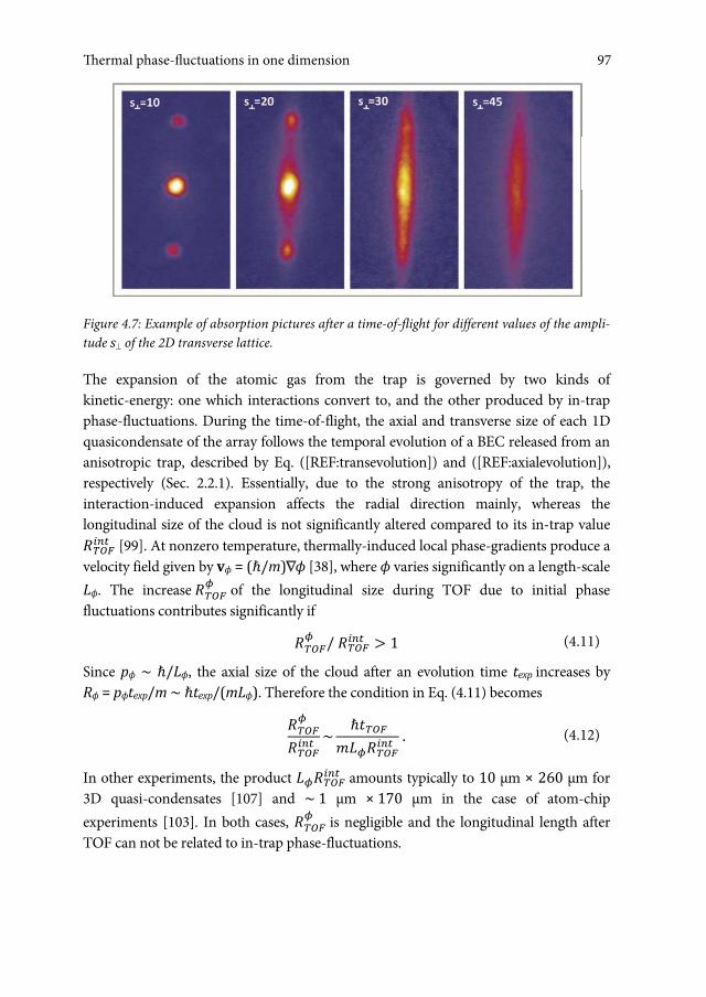
Exploring the superfluid-to-insulator transition in a lattice
97
Figure 4.7: Example of absorption pictures after a time-of-flight for different values of the ampli-tude s of the 2D transverse lattice.
The expansion of the atomic gas from the trap is governed by two kinds of kinetic-energy: one which interactions convert to, and the other produced by in-trap phase-fluctuations. During the time-of-flight, the axial and transverse size of each 1D quasicondensate of the array follows the temporal evolution of a BEC released from an anisotropic trap, described by Eq. ([REF:transevolution]) and ([REF:axialevolution]), respectively (Sec. 2.2.1). Essentially, due to the strong anisotropy of the trap, the interaction-induced expansion affects the radial direction mainly, whereas the longitudinal size of the cloud is not significantly altered compared to its in-trap value ������� [99]. At nonzero temperature, thermally-induced local phase-gradients produce a velocity field given by vϕ = (�/m)Lϕ [38], where ϕ varies significantly on a length-scale Lϕ. The increase ����� of the longitudinal size during TOF due to initial phase fluctuations contributes significantly if ����� / ������� � 1 (4.11)
Since pϕ ∼ �/Lϕ, the axial size of the cloud after an evolution time texp increases by Rϕ = pϕtexp/m ∼ �texp/(mLϕ). Therefore the condition in Eq. (4.11) becomes �����
������� ~�����
���������� . (4.12)
In other experiments, the product ��������� amounts typically to 10 μm × 260 μm for 3D quasi-condensates [107] and ∼ 1 μm × 170 μm in the case of atom-chip experiments [103]. In both cases, ����� is negligible and the longitudinal length after TOF can not be related to in-trap phase-fluctuations.
97Thermal phase-fluctuations in one dimension

Nicole Fabbri
98
Figure 4.8: (a) and (b): Profiles of the atomic cloud (red dots) at s = 5 and s = 45 compared with a fitted Gaussian and Lorentzian function, respectively (blue curves). Such profiles are ob-tained from the images in (c) and (d), by integrating the density along the vertical axis of the ab-sorption pictures, in the square defined by the green dashed line.
For our 1D lattice gases, this quantity is typically reduced to ∼ 1 μm × 27 μm for s = 5 and it decreases as the amplitude of the optical confinement increases (∼ 0.2 μm × 22 μm for s = 56). This estimate refers to a representative tube with a number of atoms equal to the average value over the entire array. Thus, one expects that for low values of s the in-trap size still dominates and the density profile has a parabolic shape as expected in the Thomas-Fermi regime, whereas for high values of s phase-fluctuations enlarge the distribution and the profile assumes a Lorentzian shape. Let us also notice that, over the whole range of s explored in the experiment, we can completely neglect the momentum-spread associated with the finite-size in this direction. 15F
16
16 The axial in-trap size of the atomic cloud is ∼ 30 μm. Thus, the associated momentum spread is Δp ∼ �H 0.03 μm-1, which corresponds to Δx ∼ 0.5 μm after time-of-flight, well below our imaging resolution.
Nicole Fabbri98
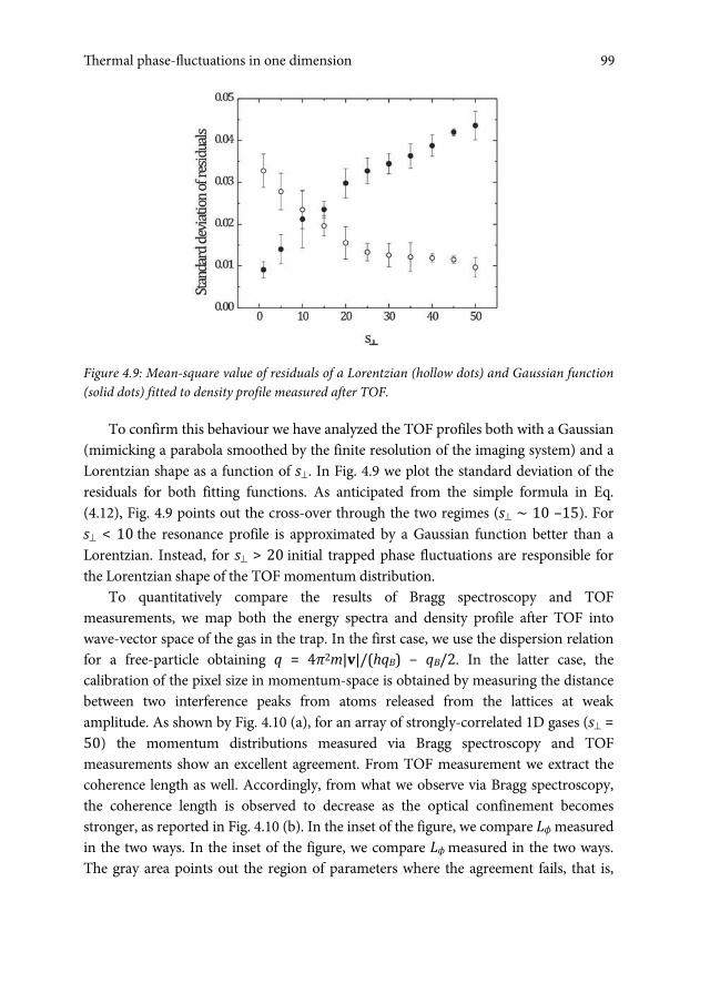
Exploring the superfluid-to-insulator transition in a lattice
99
Figure 4.9: Mean-square value of residuals of a Lorentzian (hollow dots) and Gaussian function (solid dots) fitted to density profile measured after TOF.
To confirm this behaviour we have analyzed the TOF profiles both with a Gaussian (mimicking a parabola smoothed by the finite resolution of the imaging system) and a Lorentzian shape as a function of s. In Fig. 4.9 we plot the standard deviation of the residuals for both fitting functions. As anticipated from the simple formula in Eq. (4.12), Fig. 4.9 points out the cross-over through the two regimes (s ∼ 10 –15). For s < 10 the resonance profile is approximated by a Gaussian function better than a Lorentzian. Instead, for s > 20 initial trapped phase fluctuations are responsible for the Lorentzian shape of the TOF momentum distribution.
To quantitatively compare the results of Bragg spectroscopy and TOF measurements, we map both the energy spectra and density profile after TOF into wave-vector space of the gas in the trap. In the first case, we use the dispersion relation for a free-particle obtaining q = 4π2m|v|/(hqB) – qB/2. In the latter case, the calibration of the pixel size in momentum-space is obtained by measuring the distance between two interference peaks from atoms released from the lattices at weak amplitude. As shown by Fig. 4.10 (a), for an array of strongly-correlated 1D gases (s = 50) the momentum distributions measured via Bragg spectroscopy and TOF measurements show an excellent agreement. From TOF measurement we extract the coherence length as well. Accordingly, from what we observe via Bragg spectroscopy, the coherence length is observed to decrease as the optical confinement becomes stronger, as reported in Fig. 4.10 (b). In the inset of the figure, we compare Lϕ measured in the two ways. In the inset of the figure, we compare Lϕ measured in the two ways. The gray area points out the region of parameters where the agreement fails, that is,
99Thermal phase-fluctuations in one dimension

Nicole Fabbri
100
where the TOF profiles are not dominated by the velocity field of phase-fluctuations (see Eq. (4.12)).
Figure 4.10: (a) Momentum distribution of an array of 1D gases in a strongly confining optical lattice (s = 50) measured through Bragg spectroscopy (black dots) and direct mapping in the TOF density profile (red curve). (b) Half coherence length Lϕ extracted from the TOF measure-ments is shown as a function of s on a linear scale. The gray area points out the region of pa-rameters where TOF measurements can not be used to extract Lϕ. Inset: Comparison between Lϕ from Bragg measurements (black dots) and direct mapping (red dots).
4.4 Simulating the response of the array
We now want to simulate the response of the array of 1D tubes to the Bragg excita-tion. This will allow us to verify a posteriori the assumptions we made throughout the discussion of the Bragg measurements.
Single-tube response. First, I discuss how to simulate the contribution of a single tube. From the considerations presented in Sec. 4.1.1 and 4.2, we simulate the
Nicole Fabbri100
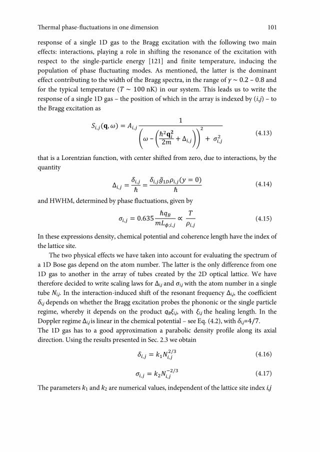
Exploring the superfluid-to-insulator transition in a lattice
101
response of a single 1D gas to the Bragg excitation with the following two main effects: interactions, playing a role in shifting the resonance of the excitation with respect to the single-particle energy [121] and finite temperature, inducing the population of phase fluctuating modes. As mentioned, the latter is the dominant effect contributing to the width of the Bragg spectra, in the range of γ ∼ 0.2 – 0.8 and for the typical temperature (T ∼ 100 nK) in our system. This leads us to write the response of a single 1D gas – the position of which in the array is indexed by (i,j) – to the Bragg excitation as
��,���, �� � ��,� 1
�� � ������
2� � �,����� ��,��
(4.13)
that is a Lorentzian function, with center shifted from zero, due to interactions, by the quantity
�,� � ��,�� � ��,�������,��� � 0�
� (4.14)
and HWHM, determined by phase fluctuations, given by
��,� � 0.��� ��������,� ∝
���,� (4.15)
In these expressions density, chemical potential and coherence length have the index of the lattice site.
The two physical effects we have taken into account for evaluating the spectrum of a 1D Bose gas depend on the atom number. The latter is the only difference from one 1D gas to another in the array of tubes created by the 2D optical lattice. We have therefore decided to write scaling laws for Δi,j and σi,j with the atom number in a single tube Ni,j. In the interaction-induced shift of the resonant frequency Δi,j, the coefficient δi,j depends on whether the Bragg excitation probes the phononic or the single particle regime, whereby it depends on the product qBξi,j, with ξi,j the healing length. In the Doppler regime Δi,j is linear in the chemical potential – see Eq. (4.2), with δi,j=4/7. The 1D gas has to a good approximation a parabolic density profile along its axial direction. Using the results presented in Sec. 2.3 we obtain ��,� � ����,��/� (4.16)
��,� � ����,���/� (4.17)
The parameters k1 and k2 are numerical values, independent of the lattice site index i,j6F16.
101Thermal phase-fluctuations in one dimension
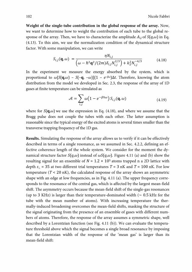
Nicole Fabbri
102
Weight of the single-tube contribution in the global response of the array. Now, we want to determine how to weight the contribution of each tube to the global re-sponse of the array. Then, we have to characterize the amplitude Ai,j of S(q,ω) in Eq. (4.13). To this aim, we use the normalization condition of the dynamical structure factor. With some manipulation, we can write
��,���, �� � ���,��� � ������2����,���,����� � �����,�����
(4.18)
In the experiment we measure the energy absorbed by the system, which is proportional to ω[S(q,ω) – S(–q, –ω)](1 – e–βω)Δt. Therefore, knowing the atom distribution from the model we developed in Sec. 2.3, the response of the array of 1D gases at finite temperature can be simulated as � ����1 � ������
�,���,���, �� (4.19)
where for S(q,ω) we use the expression in Eq. (4.18), and where we assume that the Bragg pulse does not couple the tubes with each other. The latter assumption is reasonable since the typical energy of the excited atoms is several times smaller than the transverse trapping frequency of the 1D gas.
Results. Simulating the response of the array allows us to verify if it can be effectively described in terms of a single resonance, as we assumed in Sec. 4.2.2, defining an ef-fective coherence length of the whole system. We consider for the moment the dy-namical structure factor S(q,ω) instead of ωS(q,ω). Figure 4.11 (a) and (b) show the resulting signal for an ensemble of N = 1.2 × 10⁵ atoms trapped n a 2D lattice with depth s = 35 at two different trial temperatures T = 3 nK and T = 100 nK. For low temperature (T < 20 nK), the calculated response of the array shows an asymmetric shape with an edge at low frequencies, as in Fig. 4.11 (a). The upper frequency corre-sponds to the resonance of the central gas, which is affected by the largest mean-field shift. The asymmetry occurs because the mean-field shift of the single-gas resonances (up to 3 KHz) is larger than their temperature-dominated width (∼ 0.5 kHz for the tube with the mean number of atoms). With increasing temperature the ther-mally-induced broadening overcomes the mean-field shifts, masking the structure of the signal originating from the presence of an ensemble of gases with different num-bers of atoms. Therefore, the response of the array assumes a symmetric shape, well described by a Lorentzian function (see Fig. 4.11 (b)). We can evaluate the tempera-ture threshold above which the signal becomes a single broad resonance by imposing that the Lorentzian width of the response of the ‘mean gas’ is larger than its mean-field shift:
Nicole Fabbri102
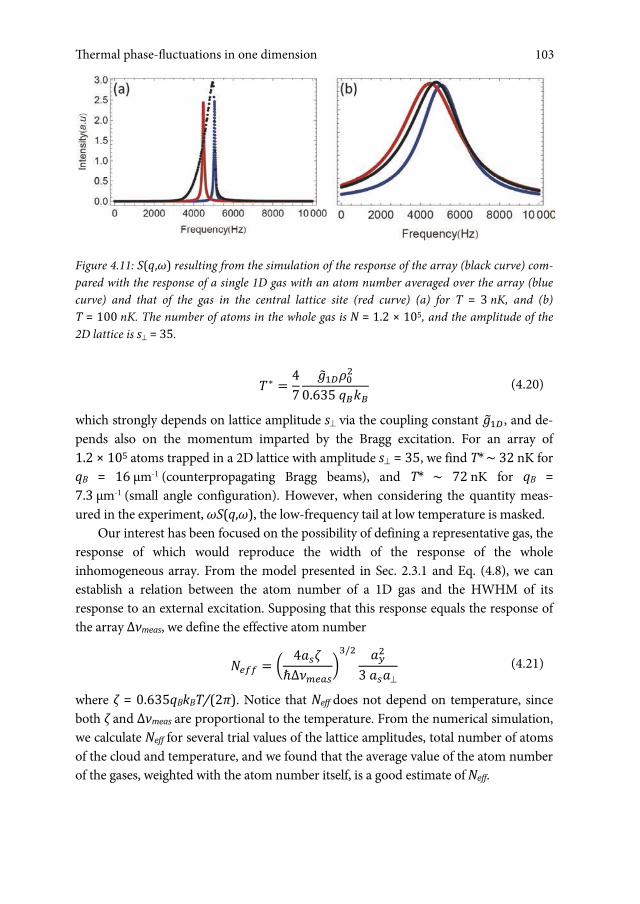
Exploring the superfluid-to-insulator transition in a lattice
103
Figure 4.11: S(q,ω) resulting from the simulation of the response of the array (black curve) com-pared with the response of a single 1D gas with an atom number averaged over the array (blue curve) and that of the gas in the central lattice site (red curve) (a) for T = 3 nK, and (b) T = 100 nK. The number of atoms in the whole gas is N = 1.2 × 10⁵, and the amplitude of the 2D lattice is s = 35.
�∗ � 4
7�������
0.635 ���� (4.20)
which strongly depends on lattice amplitude s via the coupling constant ����, and de-pends also on the momentum imparted by the Bragg excitation. For an array of 1.2 × 10⁵ atoms trapped in a 2D lattice with amplitude s = 35, we find T* ∼ 32 nK for qB = 16 μm-1 (counterpropagating Bragg beams), and T* ∼ 72 nK for qB = 7.3 μm-1 (small angle configuration). However, when considering the quantity meas-ured in the experiment, ωS(q,ω), the low-frequency tail at low temperature is masked.
Our interest has been focused on the possibility of defining a representative gas, the response of which would reproduce the width of the response of the whole inhomogeneous array. From the model presented in Sec. 2.3.1 and Eq. (4.8), we can establish a relation between the atom number of a 1D gas and the HWHM of its response to an external excitation. Supposing that this response equals the response of the array Δνmeas, we define the effective atom number
���� � � 4���������
���� ���
3 ��� (4.21)
where ζ = 0.635qBkBT/(2π). Notice that Neff does not depend on temperature, since both ζ and Δνmeas are proportional to the temperature. From the numerical simulation, we calculate Neff for several trial values of the lattice amplitudes, total number of atoms of the cloud and temperature, and we found that the average value of the atom number of the gases, weighted with the atom number itself, is a good estimate of Neff.
103Thermal phase-fluctuations in one dimension

Nicole Fabbri
104
4.5 Measure Temperature
Since Lϕ depends both on temperature and density, if one could find a good estimate of the density, one could have access to the temperature of the system. This would become a primary thermometer, i.e., a method connecting the measured quantity to temperature from first principles. For weakly-interacting ultracold gases, TOF meas-urements are an example of a primary thermometer [149], but this method does not normally give information on temperature for a lattice gas.
With this prospect, an important issue consists in establishing if the system is at thermal equilibrium, especially for s ranging from 20 to 56, where transverse tunneling is completely suppressed on the timescale of the experiment and thermalization can occur only through the dynamics in the axial direction. As a general point, trapped 1D gases with collisional point-like interactions are almost-integrable systems. In uniform 1D systems, integrability is predicted to prevent thermalization [150]. Since the number of integrals of motion equals exactly the number of degrees of freedom, the state of the system always depends on its initial state, in the course of its dynamical evolution. Actually, thermalization is forbidden in any closed system, but for non integrable systems the eigenstate thermalization hypothesis enables dephasing to mimic relaxation to the thermal equilibrium [151, 152]. Let us mention that experiments conducted in D. S. Weiss's group [109] have indicated the absence of thermalization in a trapped Tonks-Girardeau gas (γ ∼ 4), whereas for a less interacting 1D gas, as probed in our experiment (γ ∼ 0.6), re-equilibration effects have been observed on a timescale of a few tens of ms [109], comparable with the timing used in our experiment. This suggests that thermalization is prevented only for high values of γ. In addition, let us notice that the coherence length measured in our experiment is perfectly compatible with a description in terms of thermal equilibrium, according to the discussion in Sec. 4.2.2. For these reasons, we assume thermal equilibrium and thermal population of 1D modes in the 1D gases.
In the light of that, the measurement of Lϕ performed via Bragg spectroscopy allows us to evaluate the temperature of the system, according to Eq. (4.8), using the mean density. Figure 4.12 shows the estimated temperature of the array of 1D gases, obtained by the Bragg measurements at qB = 7.3 μm-1. The stronger the transverse confinement, the higher is the temperature. This increase cannot be explained as an effect of the radiation pressure of the laser light producing the optical lattice (∼ 7 nK/s for s = 35, corresponding to a few hundreds of pK on the timescale of the experiment), and it is consistent with the increase of axial confinement according to arguments presented in Sec. 4.2.2.
Nicole Fabbri104

Exploring the superfluid-to-insulator transition in a lattice
105
Figure 4.12: Measurement of the temperature of an array of 1D gases as a function of the trans-verse lattice amplitude.
4.6 Conclusions
In conclusion, we investigated the coherence properties of an array of 1D gases by measuring their momentum distribution. Since the latter shows a Lorentzian shape as predicted for a single uniform 1D gas, it was possible to define consequently an effec-tive coherence length of the whole ensemble. Its measurement showed an evident re-duction as the optical confinement was increased. We also performed a strict com-parison between Bragg spectroscopy and direct mapping of momentum distribution into density distribution after TOF. This demonstrated that TOF images give access to coherence properties in the regime of strong phase-fluctuations for s > 15. We developed a simulation of the response of the array, which allows us to verify the as-sumptions made in the analysis of the Bragg spectra. Besides, the measurement of the coherence length allowed us to give an estimate of the temperature of the array, based on the identification of an “effective” 1D gas. This measurement can represent a first step in the direction of creating multiple primary thermometers based on different theoretical approximations, and then check for their consistency at low temperatures. Our study of phase fluctuations paves the way for future studies of the coherence properties in 1D geometries with short coherence lengths. Of particular interest in our view are strongly interacting disordered systems where the role of thermal phase fluctuations in the nature of the superconductor-insulator transition is still debated [153, 154]. So far, only disordered gaseous quasi-condensates have been investigated, where was shown that the contribution of phase fluctuations is small [155, 156].
105Thermal phase-fluctuations in one dimension

Chapter 5 Exploring the superfluid-to-insulator transition in a lattice
The realization of the Bose-Hubbard model [68] with cold gases in optical lattices has been one of the corner stones in carrying out quantum simulations of solid-state physics problems using ultracold atomic samples, also with a view to implementing quantum information processes. The most remarkable fact that this model accounts for is the occurrence of an interaction-induced quantum phase-transition from a su-perfluid to a Mott insulating state. One-dimensional gases are a favourable test-ground, since the role of interactions is strongly enhanced by the one-dimensional geometry. A fundamental requirement for using such strongly-correlated gaseous systems as quantum simulators is their precise experi-mental characterization. As in the analogy of condensed-matter physics, the presence of strong correlations makes it hard to draw a complete picture, both from the ex-perimental and theoretical point of view. Various techniques have been already used to obtain information on these systems like, for instance, the presence of a gap in the spectrum of a Mott insulator [32, 31] or its shell structure [45, 157]. An important information for characterizing the system concerns elementary excitations on which the dynamical properties of the many-body system depend. In this Chapter, we re-port on the first measurement of the linear response of interacting one-dimensional Bose gases across the transition from a superfluid to a Mott-insulator [50]. Elemen-tary excitations are induced at nonzero momentum, exploiting two-photon Bragg scattering as a probe. Now the discussion will be specialized to the excitations in-duced within the lowest energy-band determined by the presence of the periodic po-tential; the excitations in higher energy-bands will be the subject of the next Chapter. From the continuous modification of the excitation-spectra, we obtain quantitative information on the critical lattice-amplitude for entering the Mott-insulting phase. The complexity of these strongly-correlated quantum-phases is directly displayed in the spectra which exhibit novel features. On the superfluid side of the transition, the presence of an extra mode in addition to the phonon mode is suggested. In the in-homogeneous Mott-insulating state, multiple resonances are observed. They give in-formation about the particle-hole gap, the inhomogeneity of the trapped system, and exhibit novel features at low energies that could be related to the temperature of the
Nicole Fabbri, Bragg spectroscopy of quantum gases: Exploring physics in one dimension isBN 978-88-6655-220-8 (print) isBN 978-88-6655-221-5 (online) © 2012 Firenze University Press

Nicole Fabbri
108
atomic sample. The value of the particle-hole gap is a particularly interesting quantity in the study of quantum critical phenomena. In addition, this gap is also very impor-tant for the practical application of these systems to quantum information process-ing, since it determines the fidelity of the Mott state [129].
5.1 Does Bragg scattering tell something more on Mott insulators?
In the last few years, different atomic insulating phases have been realized demon-strating the versatility of gaseous systems. These include bosonic Mott insulators in one-dimensional [32], two-dimensional [158] and three-dimensional [31] systems, disordered bosonic insulating phases [35] as well as fermionic Mott insulators [36, 37]. The characterization of these insulating quantum phases has revealed many of their properties. One key piece of evidence for the quantum phase transition is the loss of global phase coherence of the matter wavefunction when the lattice depth in-creases beyond a critical value. However, the loss of coherence could arise from many sources, such as quantum or thermal depletion of the condensate during the loading process. Therefore, complementary evidence for the Mott-insulator transition was provided showing the presence of a gap in the excitation spectrum by applying a po-tential gradient to the lattice [31] or by modulating the lattice which drives the system in the Mott phase [32]. Further experiments have demonstrated this gap to vanish in a disordered insulating phase [35]. A noise correlation analysis of time-of-flight pic-tures has shown the spatial order of the atomic distribution [159] and its controlled alteration when modifying the lattice potential [160]. Studies on the suppression of compressibility have been performed in fermionic [36, 37] and bosonic [161] Mott insulators. In addition to these properties expected in homogeneous insulating phases, the presence of a trap enriches the experimental situation while creating al-ternate regions of Mott insulator with different filling factors and superfluid states [68, 162]. This shell structure has been identified in experiments as clearly related to the trapping potential [45, 157]. Recently, single-site addressing has allowed one to directly measure compressibility [163] and temperature [164] of a two-dimensional Mott insulator.
In this context, Bragg spectroscopy offers the possibility of deepening our insight on correlated phases of gases in optical lattices, better characterizing the quantum phase-transition from superfluid to Mott insulator, as well as highlighting the properties of strongly-correlated superfluids. In contrast to applying a potential gradient as mentioned above, Bragg spectroscopy is not susceptible to effects like Bloch oscillations and Landau-Zener tunneling. Moreover, Bragg spectroscopy allows a tunable nonzero momentum transfer and in principle can reveal the full structure of the excitations, information unavailable using other techniques. Due to the lattice
Nicole Fabbri108

Exploring the superfluid-to-insulator transition in a lattice
109
periodicity, the amplitude of the system response is modulated by the momentum of the excitation modulus �kL [129, 130]. For a homogeneous system, an analytical expression of dynamical structure factor has been found in the framework of perturbation theory [130]:
����, �� � 32 � ������� � 1� ��� ��� �2 ������ ��� �2 �
��
���� �� � �
�� (5.1)
Here, g = N/Ns is the filling factor, i.e., the ratio of the number of particles N to the number of occupied lattice sites Ns, r = 1 ... Ns is the site index and a the lattice constant. This equation indicates that the response of the system is modulated as a function of the momentum qB of the external perturbation, and its maximum is expected at qB = π/d = kL.
Since insulating states are hard to be excited, due to the presence of the gap, the lattice-amplitude modulation experiments [32, 35], which are conducted at zero momentum-transfer, require a large modulation (typically, the 25% of the lattice amplitude). In that case, the response signal cannot be treated in the linear-response framework [165]. In contrast, by setting a favorable nonzero value of momentum, one can reduce the strength of the external perturbation exploited as a probe, keeping a reasonable signal-to-noise ratio. In Ref. [130] the validity condition for the Bragg strength is calculated for a homogeneous Mott insulator
�� � �������
��� ��� �2 �. (5.2)
No quantitative prediction is available for inhomogeneous systems, as far as we know. In the present Bragg experiment, we verify the linear response conditions to hold in practice, as illustrated in Chapter 3.
In the Mott regime the condition of linear response is fulfilled only using small amplitudes VB of the Bragg moving lattice, whereas in the superfluid phase the linear-response regime still holds for higher values of VB, due to the uncorrelated nature of the system: It is only required that the number of excited atoms be small compared to the condensate population. The spectroscopic measurement performed in the linear response regime gives direct access to the dynamical structure factor S(q,ω) of those complex phases [129, 130, 165, 166, 131, 167, 168] as described in Chapter 3.
5.1.1 The experiment
We start with an array of independent 1D gases, produced by confining a three-dimensional Bose-Einstein condensate of 87Rb atoms (N ≃ 1.5 × 10⁵ with chemical potential μ3D/h ≃ 740 Hz) in two orthogonal optical lattices with wave-
109Exploring the superfluid-to-insulator transition in a lattice
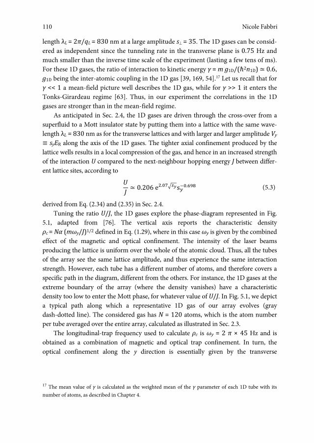
Nicole Fabbri
110
length λL = 2π/qL = 830 nm at a large amplitude s = 35. The 1D gases can be consid-ered as independent since the tunneling rate in the transverse plane is 0.75 Hz and much smaller than the inverse time scale of the experiment (lasting a few tens of ms). For these 1D gases, the ratio of interaction to kinetic energy γ = m g1D/(�2n1D) ≃ 0.6, g1D being the inter-atomic coupling in the 1D gas [39, 169, 54].17 Let us recall that for γ << 1 a mean-field picture well describes the 1D gas, while for γ >> 1 it enters the Tonks-Girardeau regime [63]. Thus, in our experiment the correlations in the 1D gases are stronger than in the mean-field regime.
As anticipated in Sec. 2.4, the 1D gases are driven through the cross-over from a superfluid to a Mott insulator state by putting them into a lattice with the same wave-length λL = 830 nm as for the transverse lattices and with larger and larger amplitude Vy ≡ syER along the axis of the 1D gases. The tighter axial confinement produced by the lattice wells results in a local compression of the gas, and hence in an increased strength of the interaction U compared to the next-neighbour hopping energy J between differ-ent lattice sites, according to
�� ≃ 0.206 e�.�����s���.��� (5.3)
derived from Eq. (2.34) and (2.35) in Sec. 2.4. Tuning the ratio U/J, the 1D gases explore the phase-diagram represented in Fig.
5.1, adapted from [76]. The vertical axis reports the characteristic density ρc = Nα (mωy/J)1/2 defined in Eq. (1.29), where in this case ωy is given by the combined effect of the magnetic and optical confinement. The intensity of the laser beams producing the lattice is uniform over the whole of the atomic cloud. Thus, all the tubes of the array see the same lattice amplitude, and thus experience the same interaction strength. However, each tube has a different number of atoms, and therefore covers a specific path in the diagram, different from the others. For instance, the 1D gases at the extreme boundary of the array (where the density vanishes) have a characteristic density too low to enter the Mott phase, for whatever value of U/J. In Fig. 5.1, we depict a typical path along which a representative 1D gas of our array evolves (gray dash-dotted line). The considered gas has N = 120 atoms, which is the atom number per tube averaged over the entire array, calculated as illustrated in Sec. 2.3.
The longitudinal-trap frequency used to calculate ρc is ωy = 2 π × 45 Hz and is obtained as a combination of magnetic and optical trap confinement. In turn, the optical confinement along the y direction is essentially given by the transverse
17 The mean value of γ is calculated as the weighted mean of the γ parameter of each 1D tube with its number of atoms, as described in Chapter 4.
Nicole Fabbri110

Exploring the superfluid-to-insulator transition in a lattice
111
confinement of the Gaussian laser beams along x and z with amplitude s = 35 which are employed to produce the 1D tubes.
Figure 5.1: Phase diagram for bosons in a one-dimensional gas with a harmonic confining po-tential along the axis of the gases. The trap has ωy /J = 0.008, length L = 100. The area marked by (I) indicates a pure superfluid phase; (II) and (III) denote inhomogeneous Mott-insulating phases: (II) is a Mott insulating phase at the center of the trap surrounded by a superfluid phase with n < 1, (III) a superfluid phase with n > 1 at the center of the trap surrounded by a Mott in-sulating phase with n = 1 and an outermost superfluid phase with n < 1. The vertical dashed green line signals the critical value of U/J for the formation of a Mott insulator with n = 1 in the homogeneous case. Gray dash-dotted curve indicates the line along which a typical micro-tube evolves with increasing amplitude of the longitudinal lattice sy (number of atoms N = 120, fre-quency of the longitudinal trap ωy = 2 π × 45 Hz). Figure is adapted from [76].
The effect of the non-uniform profile of the Gaussian laser beams creating the lattice Vy along their propagation direction (0.01 Hz) is negligible. Note that this representative gas enters the Mott region for values of U/J higher than for a homogeneous 1D gas with filling factor n = 1 (vertical dashed line). As a matter of fact, in one dimension the trapping potential has a strong effect on displacing the critical value for the formation of the Mott insulator toward larger values of U/J, much more pronounced than in higher dimensions [76].
Bragg scattering has been used to induce excitations of the system at fixed momen-tum. For this purpose, we set out an appropriate Bragg scheme as described in Sec. 3.3 to transfer a momentum �q0 close to the edge of the Brillouin zone defined by the
111Exploring the superfluid-to-insulator transition in a lattice
Nicole Fabbri
112
wave-vector kL = 2π/λL of the optical lattice where the response in the Mott state is predicted to be the largest: q0 = 0.96(3) × qL .18 Slightly different parameters (ΩB, ΔtB) have been used to obtain a good signal-to-noise ratio, keeping VB at about a one percent level of the amplitude Vy of the longitudinal lattice (for all sy values, VB < 0.15 ER).
Due to the presence of the longitudinal lattice, the excitation spectrum of the sys-tem displays a band structure. Therefore, excitation at a given quasi-momentum is as-sociated with multiple resonances corresponding to the different energy bands, as al-ready described in Sec. 3.1.2. In the experiment described here, we scan an ener-gy-range (0 – 4 kHz) corresponding to the lowest energy band n = 1. Thus, we measure ωS(q,ω), as discussed in Sec 3.2.3. In fact, when restricted to transitions within the lowest energy band, the response of the 1D gases to the scattering of light is related to terms of the type |ψ1† ψ1|2, i.e., to density-density correlation functions of the many-body state.
5.2 Characterizing the Superfluid-to-Insulator transition
In this Section, we present the results of the measurement of the dynamical structure factor across the quantum phase-transition from a superfluid to a Mott insulator state in the lowest excitation band. Let us recall that the presence of the external trapping potential crucially affects the properties of the system. As a matter of fact, when re-pulsive interaction energy overcomes the tunneling energy the Mott insulator exists even without the commensurate filling required in the non-confined case, but it does not develop uniformly along the whole of the gas. As predicted in Ref. [162], above a threshold value of U/J a first domain of insulator arises, surrounded by two tails of superfluid or normal gas on both of its sides (depending on the system entropy). Thus, rigourously speaking the gas does not experience a sharp transition but a cross-over due to coexistence of the different phases. The spectroscopic measurement we perform allows us to precisely mark the appearance of the first Mott insulating lobe. This is assumed as a boundary between the superfluid state and an inhomoge-neous Mott insulating state.
In the absence of the longitudinal lattice (sy = 0), we already demonstrated the 1D gases to be superfluids, by measuring the frequency ratio of the breathing mode to the dipole mode as in [111] (see Sec. 2.3.2). For large sy (sy > 10), the 1D gases are expected to be deeply in the inhomogeneous Mott insulating state [32].
18 The momentum imparted to the system has been calibrated as reported in Chapter 3.
Nicole Fabbri112

Exploring the superfluid-to-insulator transition in a lattice
113
Figure 5.2: Spectra in the lowest energy band measured across the transition from superfluid to Mott insulator. Solid lines are guides to the eye. The vertical dashed line in (e) marks the parti-cle-hole excitation energy Δph(qB) (see text). Note the reduction in the amplitude of the response (vertical scale).
This phase transition is reflected in a dramatic change of the dynamical structure factor of the system. This point is revealed in Fig. 5.2, which displays the excitation spectra of the system for six different amplitudes sy of the longitudinal lattice, corresponding to increasing values of the ratio U/(2J) : U/(2J) = 2.4 (sy = 4), U/(2J) = 6.3 (sy = 7), U/(2J) = 14.4 (sy = 10), U/(2J) = 30 (sy = 13), U/(2J) = 47 (sy = 15). For low sy the response exhibits a single broad resonance (see Fig. 5.2 (a-c)), whereas for large sy the spectrum shows a complex structure with multiple narrow resonances (see Fig. 5.2 (d-f)). A detailed discussion of such different resonances will be presented in Sec. 5.4. Now we are interested in highlighting the evolution of the spectra.
113Exploring the superfluid-to-insulator transition in a lattice

Nicole Fabbri
114
Figure5.3: First energy-band (blue curves) and second energy-band (green curves) of a single 1D gas for sy = 0, 2, 4, 5 (lighter colour gradations indicate increasing values of sy). The bands have been calculated in the mean-field Bogoliubov approximation for the experimental trapping fre-quencies and atom number Natom = 250. Considering a system with initial momentum distribu-tion centered on k/kL = 0 and inducing excitations with finite momentum transfer, the energy of the resonances decreases as sy increases. (b) Resonant frequency in the lowest energy band. Solid line is the frequency extracted from mean-field calculations shown in (a).
For this purpose, a Gaussian function is fitted to the whole signal-envelope corre-sponding to excitations within the energy-range corresponding to the lowest-band (δν = 0 – 4 kHz). Concerning the central frequency of the resonance at low values of sy, a shift towards lower frequencies is observed as sy increases. This can be explained tak-ing into account the Bloch-bands structure of the energy distribution of the states in the presence of a periodic potential. Figure 5.3 (a) shows a Bogoliubov mean-field calcula-tion of the energy-bands for some of the values of sy: As the amplitude of the periodic potential increases the energy bands flatten. For a momentum transfer close to the edge of the first Brillouin zone kL, this flattening implies that the resonant frequency of the transition within the lowest energy band decreases as sy increases. The frequency-shift observed in the experiment is consistent with this description (see Fig. 5.3 (b)).
A more peculiar feature of the spectra concerns their width, which exhibits non-monotonic behaviour as a function of the lattice amplitude (Fig. 5.4 (a)). For low lattice amplitudes (sy << 10), the width of the observed resonance diminishes as sy increases (see Fig. 5.2). This can again be accounted for by the same band picture mentioned above. Due to thermal effects and correlations a large distribution of quasi-momenta is populated, also at low values of sy. Therefore, the external perturbation will induce a response whose width in energy is equal to the energy bandwidth. However, the band flattens with increasing sy, and this can explain the reduction of the response width.
Nicole Fabbri114
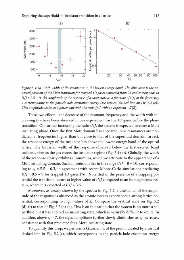
Exploring the superfluid-to-insulator transition in a lattice
115
Figure 5.4: (a) RMS width of the resonance in the lowest energy band. The blue area is the ex-pected position of the Mott transition for trapped 1D gases extracted from 76 and corresponds to U/J = 8.5 – 9. (b) Amplitude of the response of a Mott state as a function of U/J at the frequency v corresponding to the particle-hole excitation energy (see vertical dashed line on Fig. 5.2 (e)). This amplitude scales as a power-law with the ratio J/U with an exponent 1.7(3).
These two effects – the decrease of the resonant frequency and the width with in-creasing sy – have been observed in our experiment for the 1D gases before the phase transition. On further increasing the ratio U/J, the system is expected to enter a Mott insulating phase. Once the first Mott domain has appeared, new resonances are pre-dicted, at frequencies higher than but close to that of the superfluid domain: In fact, the resonant energy of the insulator lies above the lowest-energy band of the optical lattice. The Gaussian width of the response observed below the first-excited band suddenly rises as the gas enters the insulator regime (Fig. 5.4 (a)). Globally, the width of the response clearly exhibits a minimum, which we attribute to the appearance of a Mott insulating domain. Such a minimum lies in the range U/J = 8 – 10, correspond-ing to sy = 5.5 – 6.3, in agreement with recent Monte-Carlo simulations predicting U/J = 8.5 – 9 for trapped 1D gases [76]. Note that in the presence of a trapping po-tential the transition occurs at higher value of U/J compared to an homogeneous sys-tem, where it is expected at U/J = 3.61.
Moreover, as clearly shown by the spectra in Fig. 5.2, a drastic fall of the ampli-tude of the response is observed as the atomic system experiences a strong lattice po-tential, corresponding to high values of sy: Compare the vertical scale on Fig. 5.2 (d)-(f) to that of Fig. 5.2 (a)-(c). This is an indication that the system is no more a su-perfluid but it has entered an insulating state, which is naturally difficult to excite. In addition, above sy = 7, the signal amplitude further slowly diminishes as sy increases, consistent with that predicted for a Mott insulating state.
To quantify this drop, we perform a Gaussian fit of the peak indicated by a vertical dashed line in Fig. 5.2 (e), which corresponds to the particle-hole excitation energy
115Exploring the superfluid-to-insulator transition in a lattice

Nicole Fabbri
116
Δph(q0) in the Mott state (see Sec. 5.4). Instead of considering its integral, we chose to take into account its amplitude. In fact, the root-mean-squared width we observe is constant (300 Hz);19 therefore the amplitude is proportional to the integral of the signal to a good approximation. In Fig. 5.4 (b) the amplitude is plotted as a function of the ratio U/J: Fitting the experimental data with a power-law (J/U)p we find an exponent p = 1.7(3) in good agreement with the theoretical value ptheo = 2 extracted from Eq. 5.1.
5.3 Correlated superfluid in the lowest band
Even within the superfluid phase, interactions may greatly impact on the basic prop-erties, which can be revealed in the excitations of the system. In condensed-matter physics, the roton minimum in the spectrum of helium provides a well-known exam-ple of that. In this section, we would like to precisely investigate the features of corre-lated superfluid gases, i.e., by exploring the superfluid side of the transition. Again, the discussion will be specialized to excitations within the first band, using the second band only as a reference, as shown in Fig. 5.5.
In the absence of the lattice (sy = 0) and for the regime of interactions experienced by our array of 1D gases (γ = 0.6), the resonant frequency of the Lieb-Liniger model is indistinguishable from the mean-field solution within our experimental resolution. This has been demonstrated by comparison with the mean-field calculation presented in Fig. 5.2 (b) and confirmed by the calculation of the Lieb-Liniger solution kindly performed by the the group of Thierry Giamarchi [146].
Instead, the peculiar effect of the correlations in the 1D gases compared to the mean-field regime mainly consists in a modification of its shape. The case of sy = 0 –see Fig. 5.2 (a) – has been already discussed in Chapter 4. As a matter of fact, the width of the spectrum (2.5 kHz, see Fig. 5.2 (a)) is much larger than the spectrum width of the 3D BEC, which is 0.75(9) kHz for the same parameters of the Bragg excitation. This observation can be attributed to the presence of correlations and thermal effects peculiar to the beyond mean-field 1D gases. For sy > 0, a novel feature of the spectra is observed (see for instance Fig. 5.5 referring to sy = 4).
The first resonance has an asymmetric shape with a tail toward high frequencies, but the most important feature in the form of the high frequency tail is that a response signal is detected within the energy-gap between the first and the second band of the optical lattice, where in principle excitations should be forbidden, according to the
19 This width corresponds to the resolution limit of our spectroscopic tool, which is set by the time-duration of the Bragg pulse (3 ms).
Nicole Fabbri116

Exploring the superfluid-to-insulator transition in a lattice
117
conventional Bloch-band picture. For comparison, we have performed the spectroscopy on a 3D BEC loaded in an optical lattice at sy = 6 measuring a sharp resonance, falling within the bandwidth.
Figure 5.5: Spectrum of 1D gases in the SF regime (sy = 4). Solid line is a guide to the eye. Shaded areas correspond to the width of the first (blue) and second (green) lowest bands as shown in the inset.
To explain this special behaviour of the 1D lattice-gas, we consider different possible explanations.
First, the excitation spectrum is expected to differ from a mean-field description due to strong correlation [171, 172, 170, 169]. In contrast to what we discussed above, this feature is not related to the presence of the longitudinal lattice responsible for the transition from superfluid to the Mott-insulating state. As discussed in Chapter 4, the effect of interactions is enhanced in 1D gases compared to 3D even in the absence of an optical lattice.
For γ << 1, only the well-known phonon-mode responsible for superfluidity [173, 174] can be excited, according to the Bogoliubov-De Gennes mean-field approximation. For high values of γ, the Lieb-Liniger model [169] predicts umklapp excitations at finite momentum 2kF = 2πρ0, related to translations of the center of mass, with energies that tend to zero in a large system. In Fig. 5.6 (a), (b) and (c), the evolution of the dynamical structure factor S(q,ω) is reported as the parameter γ increases, namely the gas becomes more and more interacting. The horizontal axis is the wavenumber of the excitation expressed in units of the Fermi wavenumber kF = πρ0, where ρ0 is the 1D-density of the gas. The vertical axis represents energy
117Exploring the superfluid-to-insulator transition in a lattice

Nicole Fabbri
118
transfer. These density plots have been calculated in [170] with an analytic approach based on a Bethe-ansatz, and refer to systems with length L = 100 and number of atoms N = 100. Note that the 1D gas we realize corresponds to an intermediate situation between those represented in Fig. 5.6 (a) and (b) (γ = 0.6 – 0.9), where the system cannot be described anymore by a mean-field Bogoliubov-like theory. In principle, a modification of the excitation spectrum could start to become visible, expressed as an algebraic low-energy tail, in contrast to the high-energy tail observed in the experiment.
Figure 5.6: (a), (b), (c) Density plots of the dynamical structure factor computed in 170, and re-ported here for three different values of γ, i.e., the ratio of interaction energy to kinetic energy (γ = 0.25, 1, 5). The horizontal axis is momentum running up to 4 kF (kF = πρ0) and the vertical axis represents energy transfer. The data refer to systems with parameter similar to that realized in the present experiment (length L = 100, number of atoms N = 100). Momentum of excita-tions induced with our Bragg setup is indicated by red dashed lines (qB = 0.3 kF), whereas green dashed lines correspond to momentum qB = kF. (d) Profiles of the dynamical-structure factor at fixed momentum qB = kF (which correspond to cutting the previous graphs along the dashed green line) for some representative values of the interaction parameter (respectively, γ = 1, 5, 10, 20, 100). Finite experimental resolution is taken into account by using a Gaussian profile as en-ergy function, instead of δ-function. These figures are published here with the kind permission of J.-S. Caux [170].
Nicole Fabbri118
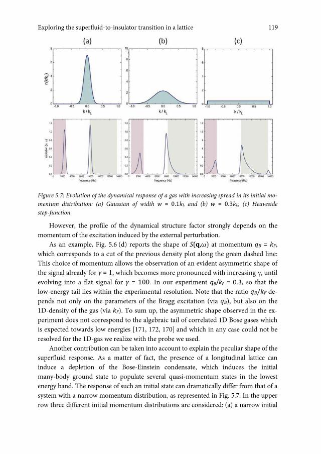
Exploring the superfluid-to-insulator transition in a lattice
119
Figure 5.7: Evolution of the dynamical response of a gas with increasing spread in its initial mo-mentum distribution: (a) Gaussian of width w = 0.1kL and (b) w = 0.3kL; (c) Heaveside step-function.
However, the profile of the dynamical structure factor strongly depends on the momentum of the excitation induced by the external perturbation.
As an example, Fig. 5.6 (d) reports the shape of S(q,ω) at momentum qB = kF, which corresponds to a cut of the previous density plot along the green dashed line: This choice of momentum allows the observation of an evident asymmetric shape of the signal already for γ = 1, which becomes more pronounced with increasing γ, until evolving into a flat signal for γ = 100. In our experiment qB/kF = 0.3, so that the low-energy tail lies within the experimental resolution. Note that the ratio qB/kF de-pends not only on the parameters of the Bragg excitation (via qB), but also on the 1D-density of the gas (via kF). To sum up, the asymmetric shape observed in the ex-periment does not correspond to the algebraic tail of correlated 1D Bose gases which is expected towards low energies [171, 172, 170] and which in any case could not be resolved for the 1D-gas we realize with the probe we used.
Another contribution can be taken into account to explain the peculiar shape of the superfluid response. As a matter of fact, the presence of a longitudinal lattice can induce a depletion of the Bose-Einstein condensate, which induces the initial many-body ground state to populate several quasi-momentum states in the lowest energy band. The response of such an initial state can dramatically differ from that of a system with a narrow momentum distribution, as represented in Fig. 5.7. In the upper row three different initial momentum distributions are considered: (a) a narrow initial
119Exploring the superfluid-to-insulator transition in a lattice
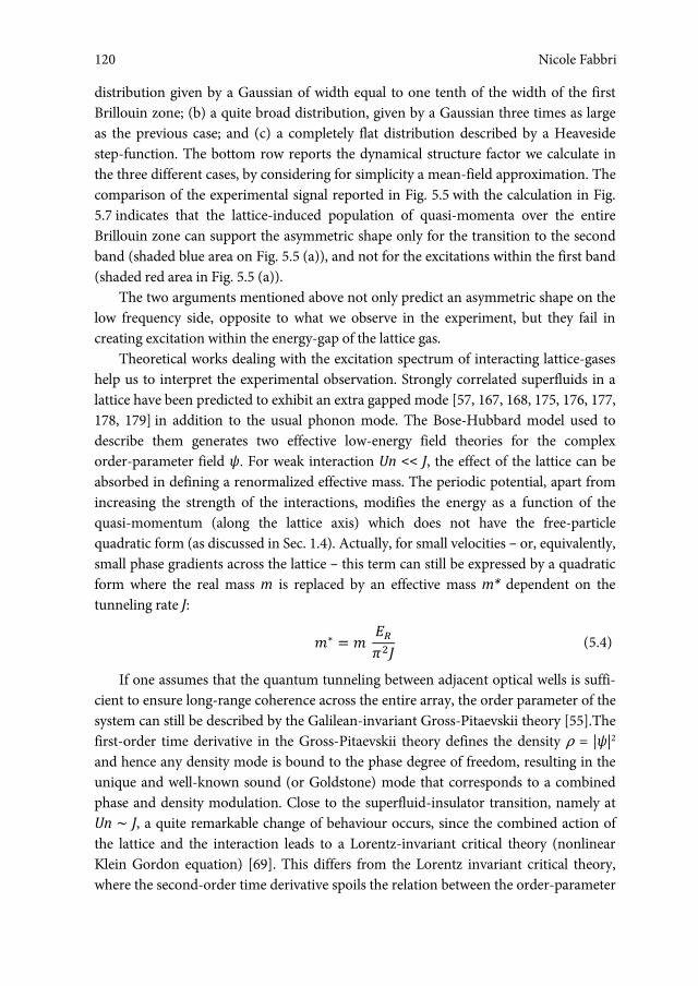
Nicole Fabbri
120
distribution given by a Gaussian of width equal to one tenth of the width of the first Brillouin zone; (b) a quite broad distribution, given by a Gaussian three times as large as the previous case; and (c) a completely flat distribution described by a Heaveside step-function. The bottom row reports the dynamical structure factor we calculate in the three different cases, by considering for simplicity a mean-field approximation. The comparison of the experimental signal reported in Fig. 5.5 with the calculation in Fig. 5.7 indicates that the lattice-induced population of quasi-momenta over the entire Brillouin zone can support the asymmetric shape only for the transition to the second band (shaded blue area on Fig. 5.5 (a)), and not for the excitations within the first band (shaded red area in Fig. 5.5 (a)).
The two arguments mentioned above not only predict an asymmetric shape on the low frequency side, opposite to what we observe in the experiment, but they fail in creating excitation within the energy-gap of the lattice gas.
Theoretical works dealing with the excitation spectrum of interacting lattice-gases help us to interpret the experimental observation. Strongly correlated superfluids in a lattice have been predicted to exhibit an extra gapped mode [57, 167, 168, 175, 176, 177, 178, 179] in addition to the usual phonon mode. The Bose-Hubbard model used to describe them generates two effective low-energy field theories for the complex order-parameter field ψ. For weak interaction Un << J, the effect of the lattice can be absorbed in defining a renormalized effective mass. The periodic potential, apart from increasing the strength of the interactions, modifies the energy as a function of the quasi-momentum (along the lattice axis) which does not have the free-particle quadratic form (as discussed in Sec. 1.4). Actually, for small velocities – or, equivalently, small phase gradients across the lattice – this term can still be expressed by a quadratic form where the real mass m is replaced by an effective mass m* dependent on the tunneling rate J:
�∗ � � ����� (5.4)
If one assumes that the quantum tunneling between adjacent optical wells is suffi-cient to ensure long-range coherence across the entire array, the order parameter of the system can still be described by the Galilean-invariant Gross-Pitaevskii theory [55].The first-order time derivative in the Gross-Pitaevskii theory defines the density ρ = |ψ|2 and hence any density mode is bound to the phase degree of freedom, resulting in the unique and well-known sound (or Goldstone) mode that corresponds to a combined phase and density modulation. Close to the superfluid-insulator transition, namely at Un ∼ J, a quite remarkable change of behaviour occurs, since the combined action of the lattice and the interaction leads to a Lorentz-invariant critical theory (nonlinear Klein Gordon equation) [69]. This differs from the Lorentz invariant critical theory, where the second-order time derivative spoils the relation between the order-parameter
Nicole Fabbri120

Exploring the superfluid-to-insulator transition in a lattice
121
modulus and the density. As a consequence, this theory allows the possibility of two in-dependent modes, which correspond to phase (Goldstone) and amplitude (Higgs) exci-tations. The latter is generated by a physically similar mechanism as the Higgs boson in high energy physics [179] and describes an exchange between condensate and non-condensate at fixed overall density. The dispersion relation of the two modes is il-lustrated in Fig. 5.8 (a): Whereas the Goldstone mode is the gapless sound (phonon) mode, the amplitude mode is gapped. As the ratio U/J increases, the strength of the correlation grows, and the amplitude of this mode increases. Finally, at the transition, the gapped amplitude-mode evolves in the Mott branch. Such two excitation modes which would not be resolved could support the asymmetry of the spectrum toward high frequencies, and especially accounting for the presence of excitation within the energy gap.
The relative strength of the two modes is predicted to be modulated by the wave-vector of the induced excitation [179, 168]. We can define a spectral weight Si of each component of the spectrum according to [179]: ���� �� � ∑ ��� ��� � ���. (5.5)
Fig. 5.8 (b) reports these weights calculated in [179] with a variational mean-field method: The sound mode dominates the response at low momenta, with the massive mode acquiring weight only for higher momenta, where the sound mode saturates.Since the probability to excite the amplitude mode is maximum at the edge of the Brillouin zone, the momentum transfer q0 = 0.96 qL chosen in the present experiment appears to be appropriate for this observation. Moreover, let us cite the calculations recently performed in Hamburg 180 describing how Goldstone and Higgs modes are modified by the presence of spatial inhomogeneity induced by the harmonic trapping potential, always present in current experiments. In particular, the breaking of the translational symmetry leads to a broadening in k-space that enlarges the signal. Reasonably, such a mechanism intervenes in our case, influencing the width of the two modes. This can be seen as a positive argument in support of the interpretation of our experimental observation in terms of the existence of two modes.
5.4 Response of an inhomogeneous Mott insulator
The response of the inhomogeneous Mott insulating phase exhibits a structure with multiple resonances (see Fig. 5.9 (c)) much more complex than that of a homogene-ous Mott insulator at zero temperature, where a single resonance corresponding to a particle-hole excitation is expected.
121Exploring the superfluid-to-insulator transition in a lattice
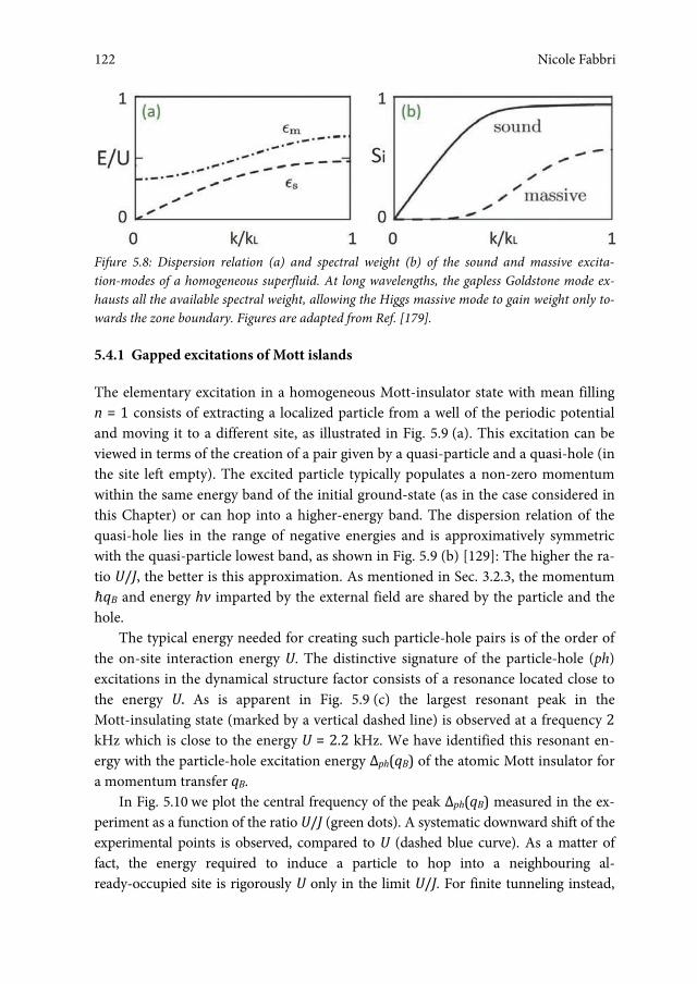
Nicole Fabbri
122
Fifure 5.8: Dispersion relation (a) and spectral weight (b) of the sound and massive excita-tion-modes of a homogeneous superfluid. At long wavelengths, the gapless Goldstone mode ex-hausts all the available spectral weight, allowing the Higgs massive mode to gain weight only to-wards the zone boundary. Figures are adapted from Ref. [179].
5.4.1 Gapped excitations of Mott islands
The elementary excitation in a homogeneous Mott-insulator state with mean filling n = 1 consists of extracting a localized particle from a well of the periodic potential and moving it to a different site, as illustrated in Fig. 5.9 (a). This excitation can be viewed in terms of the creation of a pair given by a quasi-particle and a quasi-hole (in the site left empty). The excited particle typically populates a non-zero momentum within the same energy band of the initial ground-state (as in the case considered in this Chapter) or can hop into a higher-energy band. The dispersion relation of the quasi-hole lies in the range of negative energies and is approximatively symmetric with the quasi-particle lowest band, as shown in Fig. 5.9 (b) [129]: The higher the ra-tio U/J, the better is this approximation. As mentioned in Sec. 3.2.3, the momentum �qB and energy hν imparted by the external field are shared by the particle and the hole.
The typical energy needed for creating such particle-hole pairs is of the order of the on-site interaction energy U. The distinctive signature of the particle-hole (ph) excitations in the dynamical structure factor consists of a resonance located close to the energy U. As is apparent in Fig. 5.9 (c) the largest resonant peak in the Mott-insulating state (marked by a vertical dashed line) is observed at a frequency 2 kHz which is close to the energy U = 2.2 kHz. We have identified this resonant en-ergy with the particle-hole excitation energy Δph(qB) of the atomic Mott insulator for a momentum transfer qB.
In Fig. 5.10 we plot the central frequency of the peak Δph(qB) measured in the ex-periment as a function of the ratio U/J (green dots). A systematic downward shift of the experimental points is observed, compared to U (dashed blue curve). As a matter of fact, the energy required to induce a particle to hop into a neighbouring al-ready-occupied site is rigorously U only in the limit U/J. For finite tunneling instead,
Nicole Fabbri122

Exploring the superfluid-to-insulator transition in a lattice
123
the particle-hole excitation has a minimum energy cost at zero momentum transfer Δ���� � 0� ≡ Δ��� given by [167]:
��� � ��1 � � ��� � 1� �� � �� ����. (5.6)
At the center of our 1D gases the filling factor is n = 3. Δ��� , the so-called gap of the insulating state, is smaller than U and asymptotically reaches U for large ratio U/J in the case of a homogeneous Mott insulator at zero-temperature. Actually, the gap is also modulated as a function of the momentum of the particle-hole excitation, with a minimum at qB = 0 as it is possible to infer from Fig. 5.9 (b). We compare the parti-cle-hole excitation Δph(qB) measured in the experiment to the theoretical prediction by Huber et al. [167] based on the Schwinger-boson mean-field approach (green sol-id line in Fig. 5.10). However, this calculation refers to a homogeneous Mott insulator at temperature T = 0. Our measurements of Δph(qB) are well below the prediction for the homogeneous case. This deviation can be related both to the inhomogeneity and the finite temperature affecting the particle-hole excitation energy for which no com-plete theoretical predictions exist so far.
Figure 5.9: (a) Schematics of the activation mechanism of an elementary excitation in a homo-geneous Mott insulator with filling n = 1. The required energy is of the order of U, that is, the energy-cost paid to put two atoms in the same lattice site. (b) Particle and hole dispersions in units of the tunneling parameter in a one-dimensional lattice, for U/(zJ) = 6. The horizontal arrow indicates absorption of momentum, the vertical arrow absorption of energy [129]. (c) Low energy part of the spectrum measured at sy = 13. The green solid line is a guide to the eye. The vertical dashed line indicates the particle-hole excitation frequency Δph(qB).
123Exploring the superfluid-to-insulator transition in a lattice
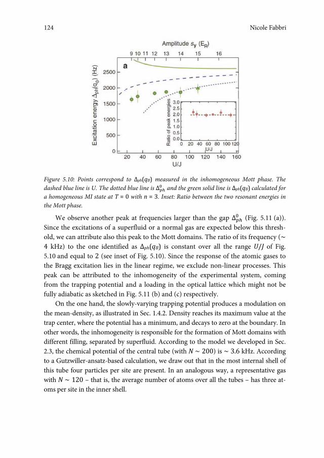
Nicole Fabbri
124
Figure 5.10: Points correspond to Δph(qB) measured in the inhomogeneous Mott phase. The dashed blue line is U. The dotted blue line is Δ��� and the green solid line is Δph(qB) calculated for a homogeneous MI state at T = 0 with n = 3. Inset: Ratio between the two resonant energies in the Mott phase.
We observe another peak at frequencies larger than the gap Δ��� (Fig. 5.11 (a)). Since the excitations of a superfluid or a normal gas are expected below this thresh-old, we can attribute also this peak to the Mott domains. The ratio of its frequency (∼ 4 kHz) to the one identified as Δph(qB) is constant over all the range U/J of Fig. 5.10 and equal to 2 (see inset of Fig. 5.10). Since the response of the atomic gases to the Bragg excitation lies in the linear regime, we exclude non-linear processes. This peak can be attributed to the inhomogeneity of the experimental system, coming from the trapping potential and a loading in the optical lattice which might not be fully adiabatic as sketched in Fig. 5.11 (b) and (c) respectively.
On the one hand, the slowly-varying trapping potential produces a modulation on the mean-density, as illustrated in Sec. 1.4.2. Density reaches its maximum value at the trap center, where the potential has a minimum, and decays to zero at the boundary. In other words, the inhomogeneity is responsible for the formation of Mott domains with different filling, separated by superfluid. According to the model we developed in Sec. 2.3, the chemical potential of the central tube (with N ∼ 200) is ∼ 3.6 kHz. According to a Gutzwiller-ansatz-based calculation, we draw out that in the most internal shell of this tube four particles per site are present. In an analogous way, a representative gas with N ∼ 120 – that is, the average number of atoms over all the tubes – has three at-oms per site in the inner shell.
Nicole Fabbri124
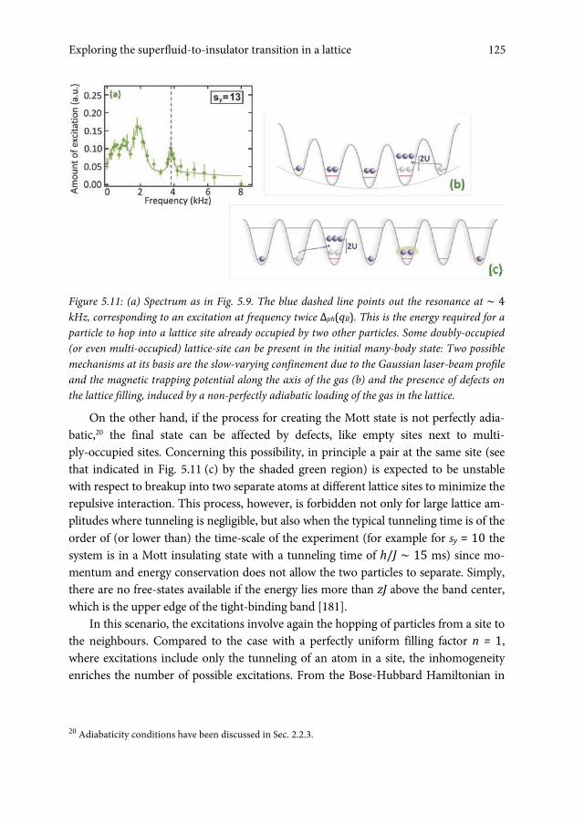
Exploring the superfluid-to-insulator transition in a lattice
125
Figure 5.11: (a) Spectrum as in Fig. 5.9. The blue dashed line points out the resonance at ∼ 4 kHz, corresponding to an excitation at frequency twice Δph(qB). This is the energy required for a particle to hop into a lattice site already occupied by two other particles. Some doubly-occupied (or even multi-occupied) lattice-site can be present in the initial many-body state: Two possible mechanisms at its basis are the slow-varying confinement due to the Gaussian laser-beam profile and the magnetic trapping potential along the axis of the gas (b) and the presence of defects on the lattice filling, induced by a non-perfectly adiabatic loading of the gas in the lattice.
On the other hand, if the process for creating the Mott state is not perfectly adia-batic,20 the final state can be affected by defects, like empty sites next to multi-ply-occupied sites. Concerning this possibility, in principle a pair at the same site (see that indicated in Fig. 5.11 (c) by the shaded green region) is expected to be unstable with respect to breakup into two separate atoms at different lattice sites to minimize the repulsive interaction. This process, however, is forbidden not only for large lattice am-plitudes where tunneling is negligible, but also when the typical tunneling time is of the order of (or lower than) the time-scale of the experiment (for example for sy = 10 the system is in a Mott insulating state with a tunneling time of h/J ∼ 15 ms) since mo-mentum and energy conservation does not allow the two particles to separate. Simply, there are no free-states available if the energy lies more than zJ above the band center, which is the upper edge of the tight-binding band [181].
In this scenario, the excitations involve again the hopping of particles from a site to the neighbours. Compared to the case with a perfectly uniform filling factor n = 1, where excitations include only the tunneling of an atom in a site, the inhomogeneity enriches the number of possible excitations. From the Bose-Hubbard Hamiltonian in
20 Adiabaticity conditions have been discussed in Sec. 2.2.3.
125Exploring the superfluid-to-insulator transition in a lattice
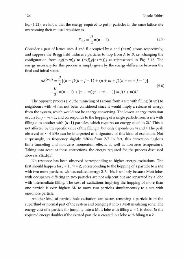
Nicole Fabbri
126
Eq. (1.22), we know that the energy required to put n particles in the same lattice site overcoming their mutual repulsion is
���� � �2 ��� � 1�. (5.7)
Consider a pair of lattice sites A and B occupied by n and (n+m) atoms respectively, and suppose the Bragg field induces j particles to hop from A to B, i.e., changing the configuration from nA;(n+m)B to (n+j)A;(n+m‐j)B as represented in Fig. 5.12. The energy necessary for this process is simply given by the energy-difference between the final and initial states:
������ � �2 ��� � ���� � � � 1� � �� � � � ���� �� � � � 1��
��2 ���� � 1� � �� � ���� � � � 1�� � ��� � ���. (5.8)
The opposite process (i.e., the tunneling of j atoms from a site with filling (n+m) to neighbours with n) has not been considered since it would imply a release of energy from the system, which would not be energy-conserving. The lowest-energy excitation occurs for j = m = 1, and corresponds to the hopping of a single particle from a site with filling n to another with (n+1) particles, which requires an energy equal to 2U. This is not affected by the specific value of the filling n, but only depends on m and j. The peak observed at ∼ 4 kHz can be interpreted as a signature of this kind of excitation. Not surprisingly, its frequency slightly differs from 2U. In fact, this derivation neglects finite-tunneling and non-zero momentum effects, as well as non-zero temperature. Taking into account these corrections, the energy required for the process discussed above is 2Δph(qB).
No response has been observed corresponding to higher-energy excitations. The first should happen for j = 1, m = 2, corresponding to the hopping of a particle to a site with two more particles, with associated energy 3U. This is unlikely because Mott lobes with occupancy differing in two particles are not adjacent but are separated by a lobe with intermediate filling. The cost of excitations implying the hopping of more than one particle is even higher: 6U to move two particles simultaneously to a site with one-more particle.
Another kind of particle-hole excitation can occur, removing a particle from the superfluid or normal part of the system and bringing it into a Mott insulating zone. The energy cost of a particle for jumping into a Mott lobe with filling n = 1 is about U; the required energy doubles if the excited particle is created in a lobe with filling n = 2.
Nicole Fabbri126
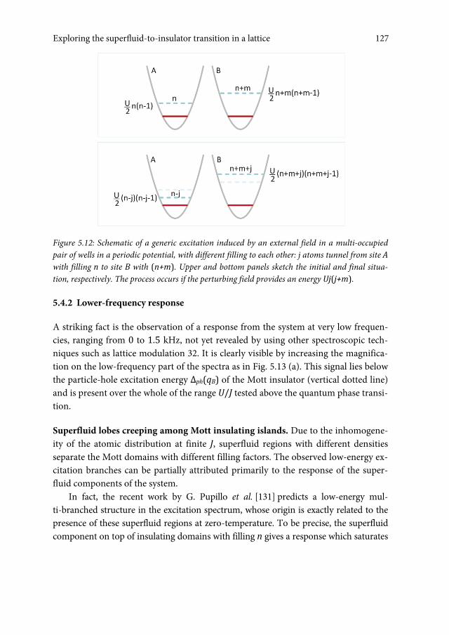
Exploring the superfluid-to-insulator transition in a lattice
127
Figure 5.12: Schematic of a generic excitation induced by an external field in a multi-occupied pair of wells in a periodic potential, with different filling to each other: j atoms tunnel from site A with filling n to site B with (n+m). Upper and bottom panels sketch the initial and final situa-tion, respectively. The process occurs if the perturbing field provides an energy Uj(j+m).
5.4.2 Lower-frequency response
A striking fact is the observation of a response from the system at very low frequen-cies, ranging from 0 to 1.5 kHz, not yet revealed by using other spectroscopic tech-niques such as lattice modulation 32. It is clearly visible by increasing the magnifica-tion on the low-frequency part of the spectra as in Fig. 5.13 (a). This signal lies below the particle-hole excitation energy Δph(qB) of the Mott insulator (vertical dotted line) and is present over the whole of the range U/J tested above the quantum phase transi-tion.
Superfluid lobes creeping among Mott insulating islands. Due to the inhomogene-ity of the atomic distribution at finite J, superfluid regions with different densities separate the Mott domains with different filling factors. The observed low-energy ex-citation branches can be partially attributed primarily to the response of the super-fluid components of the system.
In fact, the recent work by G. Pupillo et al. [131] predicts a low-energy mul-ti-branched structure in the excitation spectrum, whose origin is exactly related to the presence of these superfluid regions at zero-temperature. To be precise, the superfluid component on top of insulating domains with filling n gives a response which saturates
127Exploring the superfluid-to-insulator transition in a lattice

Nicole Fabbri
128
at energy 4nJ. This structure emerges both in quantum Monte-Carlo simulations and in analytic calculations based on an extended-fermionization model.21 The density pro-file can be visualized as being composed of stacked horizontal layers. Since atoms are no longer frozen, the layers are not independent. However, if number-fluctuations in adjacent layers do not overlap in space, all of them can be treated independently and standard fermionization techniques can be applied to each layer separately, as in the homogeneous system. In this situation single-particle solutions provide expressions for all many-body observable quantities. In the low density limit n = 1, the extend-ed-fermionization method reduces to standard fermionization, as depicted in Fig. 5.13 (b) drawn from [131]. The Figure reports the dynamical structure factor of a one-dimensional gas at fixed momentum transfer 0��� �kL. It refers specifically to a low-filling factor case n = 2. The feature of the spectrum is strongly affected by the wave-vector of the induced excitation: As a comparison the inset shows S(qB,ω) at low-er transferred momentum, increasing from the top to the bottom (0�2 �kL, 0�4�kL, 0���kL). For low momentum, a response at �ω/J < 4 is expected. It is solely due to the small number of atoms in the sites which are in the superfluid phase, thus correspond-ing to excitations of the borders of the atomic gas. If the Bragg field imparts a momen-tum at the boundary of the first Brillouin zone of the longitudinal lattice as in Fig. 5.13 (b) – that is the scheme implemented in our experiment – excitations are predicted up to 8J. The value 4J corresponds to the single particle band width of a hole, that is, of an empty site tunneling in the lattice. These excitations are thus due to the coupling be-tween the ground state and eigenstates with at most one atom per site. The peak at �ω/J = 8 corresponds to excitations in the superfluid with more than two atoms per site.
This treatment can be simply extended to fit the situation we realize in the experiment. As already mentioned in the last section, we calculated to have up to four particles per site, in the central tube of the array. In this tube, the inner shell is in an insulating state. Thus, the highest-density superfluid component is seated on a Mott pedestal with mean filling equal to 3. Its response is expected at 12J. Globally, the superfluid part of the whole gas contributes to the system response with a complex structure of multiple peaks, stretched out in the energy-range 4 J – 12 J. The observed spectrum clearly exhibits a response in the frequency range matching those excitations – see shaded pink area in Fig. 5.13 (a). However, in the experiment, it is not possible to resolve separately each peak, since they are separated from each other by 130 Hz, less than an half the experimental resolution (300 Hz). Thus, the superfluid response should be given by the convolution of the multi-branched structure with a Gaussian
21 This is a generalization of the Fermi-Bose mapping, in the presence of a multi-component gas [131].
Nicole Fabbri128

Exploring the superfluid-to-insulator transition in a lattice
129
function whose width should be determined by the resolution, but this profile is altered by the presence of a signal at slightly higher frequency, which we will discuss in the next paragraph.
Figure 5.13: (a) Magnification of the low-frequency part of the spectrum in Fig. 5.9 (c) and 5.11 (a). The shaded area indicates the range where a response from the superfluid lobes is ex-pected 166, 131, corresponding to the energy interval 4 J – 12 J. For reference, also Δph(q = 0) has been indicated (vertical dotted line). (b) Dynamical structure factor of a one-dimensional gas is reported as a function of the frequency ω in units of J/�, for a fixed value of momentum 0.9 �kL 131. The gas considered consists of 64 atoms and has U/J = 8, realized in the experiment when sy = 5.5. The solid (red) and dashed (black) lines are the quantum-Monte Carlo and ex-tended-fermionization results, respectively. Inset: Dynamical structure factor of the same system at different momenta (0.2, 0.4, 0.7 �kL – top to bottom).
Additional signal. In the Mott insulator regime, a signal has been revealed also in the energy range of 0.5 – 1.5 kHz (gray area in Fig. 5.13 (a)). Even if these resonances are below the energy particle-hole gap Δph(qB) of the Mott insulator, they can not be at-tributed to the superfluid domains since their energy is too high [50].
In a uniform Mott insulator, whereas the particle-hole energy gap (i.e., the difference in energy between the ground-state and the particle-hole excitations) is of the order of U, the energy splitting between different excitations must be a fraction of the bandwidth, namely it is of the order of the tunneling energy J. Several of these modes can be simply activated by the effect of finite temperature. In particular, we can assume that in our system thermal energy overcomes J, since the characteristic temperature associated with tunneling is of the order of nanoKelvin, in a Mott insulating state.22 At thermal equilibrium, the occupation number of modes can be
22 For a lattice gas with sy = 13, whose spectrum is shown in Fig. 5.13 (a), from Eq. (2.35) we obtain J/kB = 1.6 nK.
129Exploring the superfluid-to-insulator transition in a lattice
Nicole Fabbri
130
estimated as Nj = kBT/εj,23 where εj is the energy of an excitation and kB the Boltzmann constant. Thus we expect excitations to be populated up to an energy kBT. That mechanism can explain the system response at energies larger than 12 J. Yet, how to extract a quantitative temperature from the position and/or width of these low-energy excitations is not clear. We hope that these measurements will trigger a new interest in working out such a possible relation. However, as an upper limit, the temperature corresponding to the gap is about 102 nK (marked by vertical dashed line in Fig. 5.13 (a)).24
5.5 Conclusions
In conclusion, this Chapter has presented the first measurement of the linear re-sponse of one-dimensional gases across the quantum phase cross-over from the su-perfluid state to an inhomogeneous Mott insulator state. The latter has been realized by transferring atoms in a strong optical lattice along the axial direction of the mi-cro-tubes in order to increase atom-atom interactions compared to the kinetic energy associated with tunneling between adjacent sites. Inducing excitations within the lowest energy band of the lattice, we have measured the dynamical structure factor of the system.
The dynamical structure factor has revealed a composite structure reflecting the complexity of such correlated quantum phases. Its evolution has allowed us to identify the threshold value of interactions at which the system enters an insulator state. Due to the external trapping potential, this state is made up of an insulating region alternated by superfluid lobes.
Below the transition, in addition to the sound-mode the presence of a gapped mode not completely resolved has been suggested. This is expected for strongly correlated superfluids in proximity to the transition, having been indicated as a precursor of the Mott insulating phase.
Above the transition, in Sec. 5.4 we have demonstrated that information about a non-uniform filling of the Mott state is directly accessible using Bragg spectroscopy. The trapping potential is in fact responsible for the existence of several Mott and superfluid regions in each gas. This scenario allows a variety of possible excitations in the insulating islands, since a particle can hop to a site already multiply occupied. Thus, the presence of a multiply peaked structure we have observed in the excitation
23 Note that this picture completely neglects the existence of quantum fluctuations. 24 Considering again a lattice-gas with sy = 13, from Eq. (2.34) we obtain U/kB = 97 nK.
Nicole Fabbri130

Exploring the superfluid-to-insulator transition in a lattice
131
spectrum of the system is clear evidence of the existence of a shell-like atomic density distribution. The inhomogeneity is also the origin of a response at extremely low frequencies because of the sensitivity to the presence of superfluid. Even if Bragg scattering has provided a probe of global properties of the system, since it cannot distinguish spatially different lattice sites, the measurement performed in the experiment has suggested that it can also give information about the atomic density shell-structure in a quadratic potential. Moreover, extra-signal exhibited by the spectra can be interpreted as a signature of thermally-activated particle-hole excitations. In the future, a systematic investigation of the observed novel features combined with new theoretical input should allow the addressing of open questions regarding those strongly correlated gaseous phases. Of course this calculation should also include temperature, which, as highlighted by the measurements reported in this Chapter, is expected to be very important in determining the response of an inhomogeneous Mott insulating state.
131Exploring the superfluid-to-insulator transition in a lattice

Chapter 6 Interband spectroscopy in a lattice
The presence of a periodic lattice potential remarkably enriches the scenario of possi-ble excitations that may be activated in a system. Indeed, in any periodic system, it is possible to populate several states corresponding to different bands by imparting a given momentum to the system. In Chapter 5 we investigated the excitations of one dimensional gases in the lowest energy band of the lattice potential present along its axis, characterizing the transition from a superfluid to a Mott insulator state. In this Chapter, we present two experiments which exploit high band Bragg spectroscopy.
A first preparatory experiment [132] investigates a relatively simple system, such as a three dimensional weakly interacting Bose Einstein condensate immersed in a one dimensional optical lattice. The response of the BEC in the superfluid phase is drastically modified by the presence of the lattice [182, 183, 184, 185, 186], both by the opening of energy gaps in the energy spectrum and by the change of the linear dispersion relation (and thus sound velocity) of the superfluid. In the mean field re-gime of interactions these peculiar features of the excitations of a superfluid BEC in the presence of an optical lattice are captured by the Bogoliubov theory [38]. The ex-periment demonstrates in practice the possibility to excite different bands of the lat-tice, analogously to the Bloch bands for single particles that have also been investigat-ed using cold atomic gases [102]. Moreover, we compare the inter band spectroscopy with the band calculation in the Bogoliubov De Gennes approximation.
In a second experiment [187, 188], high-band Bragg spectroscopy has been used to investigate short range phase coherence in a one dimensional gaseous Mott insula-tor. Examples of correlation induced loss of coherence can be recognized in low di-mensional systems (e.g., 1D Bose gases in the Tonks Girardeau regime [33, 34]) or in the presence of optical lattices (e.g., Mott insulator). In this framework, our interest has been focused on the regime where the phase coherence is not completely de-stroyed. A ‘perfect’ Mott state (obtained when the ratio of the Bose Hubbard parame-ters U/J is infinite) exhibits no phase coherence and is well understood. More chal-lenging is the case of Mott insulator states at finite U/J where short range coherence between a few lattice sites exists. The situation results from the coherent admixture of particles and holes on top of the Mott ground state. In this work, we propose and re-
Nicole Fabbri, Bragg spectroscopy of quantum gases: Exploring physics in one dimension isBN 978-88-6655-220-8 (print) isBN 978-88-6655-221-5 (online) © 2012 Firenze University Press
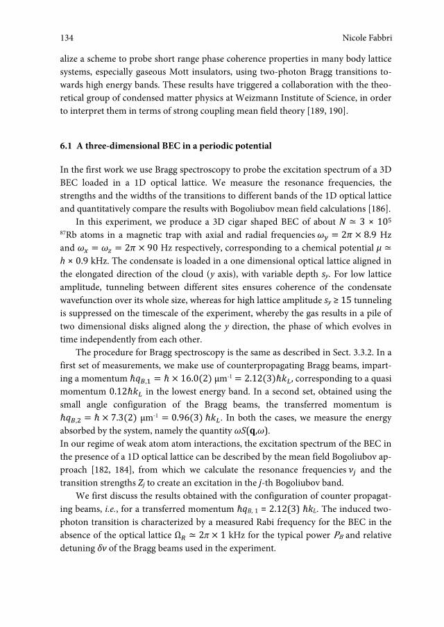
Nicole Fabbri
134
alize a scheme to probe short range phase coherence properties in many body lattice systems, especially gaseous Mott insulators, using two-photon Bragg transitions to-wards high energy bands. These results have triggered a collaboration with the theo-retical group of condensed matter physics at Weizmann Institute of Science, in order to interpret them in terms of strong coupling mean field theory [189, 190].
6.1 A three-dimensional BEC in a periodic potential
In the first work we use Bragg spectroscopy to probe the excitation spectrum of a 3D BEC loaded in a 1D optical lattice. We measure the resonance frequencies, the strengths and the widths of the transitions to different bands of the 1D optical lattice and quantitatively compare the results with Bogoliubov mean field calculations [186].
In this experiment, we produce a 3D cigar shaped BEC of about N ≃ 3 × 10⁵ 87Rb atoms in a magnetic trap with axial and radial frequencies �� � 2� � �.9 Hz and �� � �� � 2� � 90 Hz respectively, corresponding to a chemical potential μ ≃ h × 0.9 kHz. The condensate is loaded in a one dimensional optical lattice aligned in the elongated direction of the cloud (y axis), with variable depth sy. For low lattice amplitude, tunneling between different sites ensures coherence of the condensate wavefunction over its whole size, whereas for high lattice amplitude sy ≥ 15 tunneling is suppressed on the timescale of the experiment, whereby the gas results in a pile of two dimensional disks aligned along the y direction, the phase of which evolves in time independently from each other.
The procedure for Bragg spectroscopy is the same as described in Sect. 3.3.2. In a first set of measurements, we make use of counterpropagating Bragg beams, impart-ing a momentum ���,� � � � 1�.0�2� μm-1 � 2.12�3����, corresponding to a quasi momentum 0.12��� in the lowest energy band. In a second set, obtained using the small angle configuration of the Bragg beams, the transferred momentum is ���,� � � � �.3�2� μm-1 � 0.9��3� ���. In both the cases, we measure the energy absorbed by the system, namely the quantity ωS(q,ω). In our regime of weak atom atom interactions, the excitation spectrum of the BEC in the presence of a 1D optical lattice can be described by the mean field Bogoliubov ap-proach [182, 184], from which we calculate the resonance frequencies �� and the transition strengths Zj to create an excitation in the j-th Bogoliubov band.
We first discuss the results obtained with the configuration of counter propagat-ing beams, i.e., for a transferred momentum �qB, 1 � 2.12(3) �kL. The induced two-photon transition is characterized by a measured Rabi frequency for the BEC in the absence of the optical lattice Ω� ≃ 2p � 1 kHz for the typical power PB and relative detuning δν of the Bragg beams used in the experiment.
Nicole Fabbri134

Interband spectroscopy in a lattice
135
A typical Bragg spectrum is presented in Fig. 6.1 (a) corresponding to a lattice height sy = (22 ± 2). The spectrum exhibits multiple resonances corresponding to the creation of excitations in the different Bogoliubov bands as shown in Fig. 6.1 (b). These bands have been identified by comparing them with Bogoliubov calculations, as explained below, but also via a band mapping technique which we will describe in Sec. 6.1.2.
Figure 6.1: (a) Measured BEC excitation spectrum in the presence of a lattice with height sy = (22 ± 2). The increase Δσ of the width of the atomic density distribution after time-of-flight is monitored as a function of the relative detuning δν between the two counterpropagating Bragg beams. The data are fitted with Gaussian functions (gray line). The arrows below the resonances indicate the corresponding bands, represented in (b) with the same colors (numbers). (b) Band structure of the excitation spectrum of a BEC in a 1D optical lattice with sy = 22: First, second, third and fourth bands are represented (black (I), blue (II), red (III) and green (IV) lines, respec-tively). The arrows indicate processes that start from a BEC at k = 0 and induce the creation of excitations with a quasi momentum 0.12 �kL in the different bands.
135Inter-band spectroscopy in a lattice

Nicole Fabbri
136
Figure 6.2: (a) Band spectroscopy of a BEC in the presence of a 1D optical lattice: The energy of the resonances is reported as a function of the height sy of the lattice. The experimental points (blue squares, red circles and green diamonds) are compared with the numerical calculation of the Bogoliubov spectrum in the presence of a 1D lattice (solid lines) and the single particle Bloch spectrum (dashed lines). The lines correspond to the energy of an excitation in the second (blue (II) line), third (red (III) line) and fourth (green (IV) line) Bogoliubov bands. Inset of (a): Zoom of the graph (a) for low values of sy. (b) Relative strength of the excitations in the j = 2, j = 3 and j = 4 bands. Symbols and colors are the same as in (a).
Since the central frequencies of the observed resonances largely overcome their width (e.g., for sy = 22, the central frequency of the first resonance is ν1 ∼ 23 kHz, and its half width at half maximum is ∼ 1.1 kHz), ωS(q,ω) is indistinguishable from S(q,ω) within the experimental resolution, the latter being expected to have a Gauss-ian profile [121]. From a Gaussian fit of the observed resonances we extract the cen-tral frequency, the width and the relative strength of the transition towards the corre-
Nicole Fabbri136

Interband spectroscopy in a lattice
137
sponding band. In Fig. 6.2 (a), we plot the energy values corresponding to the meas-ured central frequencies as a function of sy. The vertical error bars come from the re-sult of the fitting procedure while the horizontal error bars correspond to possible systematic errors in the lattice calibration (estimated ≤ 10%). For large enough am-plitude sy of the periodic potential we observe up to three different resonances.
6.1.1 Comparison with Bogoliubov bands
The experimental data has been compared with the numerical results of a Bogoliubov calculation (solid lines in Fig. 6.2 (a)). In particular, for low amplitudes of the 1D lat-tice (sy < 6) the agreement of the resonance energies with the Bogoliubov bands (full lines) is better than with the single particle (dashed lines) Bloch bands (see inset in Fig. 6.2 (a)). For larger amplitude of the 1D lattice, we can not explicitly distinguish between the Bogoliubov and Bloch results. This comes from the experimental uncer-tainty on the calibration of the lattice amplitude.
Over the entire range of sy values used in this work, we observe a resonance cor-responding to an excitation created in the third band j = 3 (red circles in Fig. 6.2). For larger lattice amplitudes two other resonances appear, respectively for sy > 4 and sy > 20, corresponding to an excitation in the j = 2 band (blue squares in Fig. 6.2 (a)) and in the j = 4 band (green diamonds in Fig. 6.2 (a)). This demonstrates the possibility to excite, in a periodic system, several states for a given momentum transfer [102]. For weak optical lattices, the most efficient process consists of creating an excitation in the j = 3 band since the excitation energy of this band is continuously connected as sy = 0 to that of the BEC in the absence of the 1D optical lattice at the transferred momentum �qB,1 =2�12 �kL. On the contrary, the possibility to excite states in the second and fourth bands of the optical lattice requires a large enough amplitude sy. These observations can be quantified in terms of the strength Zj of the different exci-tations, which can be extracted from the energy spectrum. The strengths Zj are pro-portional to the integral ��� ����, �� with Sj(q,ω) being the structure factor corre-sponding to the creation of an excitation in the Bogoliubov band j [184]. From Eq. ([REF:deltaE3]) and assuming that ωj is much larger than the width of the resonances of Sj(q,ω), we obtain
����� � ��� ����, �� � 1�� ��� ����, �� � �� (6.1)
In the experiment, we extract the quantity fj from a Gaussian fit of the different resonances. Normalizing the sum of these quantities to one for the first three ob-served resonances (f2 + f3 + f4 = 1) allows direct comparison with the relative strengths Zj/(Z2 + Z3 + Z4) for j = 2, 3, 4. Comparison between the experimental data and the calculation reveals a reasonable agreement (see Fig. 6.2 (b)).
137Inter-band spectroscopy in a lattice

Nicole Fabbri
138
Figure 6.3: Rms width of the resonances j = 2 (blue squares) and j = 3 (red circles) as a function of sy. The gray region corresponds to the experimental rms width (with its uncertainty) for the BEC in the absence of the lattice (sy = 0). The blue (II) and red (III) lines are, respectively, the bandwidth of the second and the third band, calculated in the mean field Bogoliubov approach.
Figure 6.4: (a) Excitation spectrum of a BEC in the presence of a 1D lattice with height sy = 11 at a transferred momentum 0.96 �kL along the y direction. The arrows indicate the corresponding bands, represented in (b) with the same colors. (b) Resonance energy in the band j = 1 (black cir-cle), j = 2 (blue squares) and j � 3 (red circles) as a function of the transferred quasi momentum for a fixed value of the lattice height sy = (11 ± 1). The experimental points are compared with the Bogoliubov bands for sy = 11 (black (I), blue (II) and red (III) dashed lines); the solid lines correspond to the bands for sy = 10 and sy = 12 to take into account the 10% uncertainty of sy.
Nicole Fabbri138

Interband spectroscopy in a lattice
139
From the Gaussian fit of the experimental spectra (see Fig. 6.1 (a)), we also ex-tract the rms width of the resonances j = 2 and j = 3 with the results plotted in Fig. 6.3. Different sources can contribute to enlarge the observed resonances. In the ab-sence of an optical lattice (sy = 0), finite size Doppler broadening and mean field broadening [121] give a width of (0.36 ± 0.11) kHz, in agreement with the expected value ≃ 0.26 kHz. However, the largest contribution is introduced by the Bragg spec-troscopic scheme, essentially due to power broadening (ΔνP ≃ 1 kHz).25 The total resonance width can be obtained by quadratically adding up all these rms contribu-tions. In the presence of the optical lattice we observe that the widths of the reso-nances corresponding to the excitations in the bands j = 2 and j = 3 lie within the ex-perimental range of the resolution as expected for a coherent system, except in the case of j = 3 for large amplitudes of the lattice (sy > 20) where the width is much larg-er. We attribute these larger widths at high amplitude of the 1D lattice to the long tunneling times (∼ 0.11 s for sy = 20) implying that the system is not fully coherent along the y direction on the time scale of the experiment. The loss of coherence spreads the population of quasi momenta across a larger fraction of the Brillouin zone and, for large amplitude sy, one expects the width of the resonances to approach the bandwidths. In Fig. 6.3 we have plotted the bandwidths of the j = 2 and j = 3 bands (blue (II) and red (III) straight lines). At sy = 27 the width of the resonance j = 3 equals the bandwidth confirming this interpretation.
We also perform the experiment with a different configuration of the Bragg beams corresponding to imparting a momentum �qB,2 = 0.�6 �kL along the y axis. In Fig. 6.4 (a) an excitation spectrum in the presence of an optical lattice of height sy = 11 is depicted. Note that a first resonance at low frequency is visible correspond-ing to an excitation with non zero momentum within the lowest energy band (j = 1). Such a resonance is not observed using counter propagating Bragg beams because the strength of this transition is negligible for �qB, 1 = 2.12 �kL. Since the momentum of the excitation has been changed from the previous measurements, the resonance fre-quencies are shifted according to the dispersion relation of the different energy bands of the system. In Fig. 6.4 (b) we report the frequency of the resonances j = 1, j = 2 and j = 3 for the two values of quasi momentum used in the experiment (0.12 �kL and 0.�6 �kL). The region included between the straight lines indicates the experimental uncertainty, related to the lattice calibration. The experimental points are in good agreement with the numerical calculation of the Bogoliubov bands for sy = 11 (dashed lines in the Figure) within the error bars.
25 The broadening resulting from the atom-light interaction time (Δνt ≃ 167 Hz) is negligible.
139Inter-band spectroscopy in a lattice
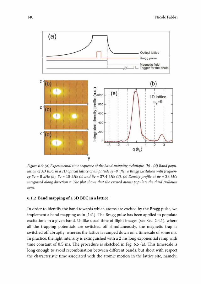
Nicole Fabbri
140
Figure 6.5: (a) Experimental time sequence of the band-mapping technique. (b) - (d) Band popu-lation of 3D BEC in a 1D optical lattice of amplitude sy=9 after a Bragg excitation with frequen-cy δv = 8 kHz (b), δv = 15 kHz (c) and δv = 37.4 kHz (d). (e) Density profile at δv = 38 kHz integrated along direction z: The plot shows that the excited atoms populate the third Brillouin zone.
6.1.2 Band mapping of a 3D BEC in a lattice
In order to identify the band towards which atoms are excited by the Bragg pulse, we implement a band mapping as in [141]. The Bragg pulse has been applied to populate excitations in a given band. Unlike usual time of flight images (see Sec. 2.4.1), where all the trapping potentials are switched off simultaneously, the magnetic trap is switched off abruptly, whereas the lattice is ramped down on a timescale of some ms. In practice, the light intensity is extinguished with a 2 ms long exponential ramp with time constant of 0.5 ms. The procedure is sketched in Fig. 6.5 (a). This timescale is long enough to avoid recombination between different bands, but short with respect the characteristic time associated with the atomic motion in the lattice site, namely,
Nicole Fabbri140

Interband spectroscopy in a lattice
141
the inverse of the bandwidth of the lowest energy band (see Sec. 2.2.3). Therefore, the band population is preserved and the quasi momentum states of the lattice gas are projected onto momentum states of the free particles released from the trap. After a time of flight of the atomic cloud (typically, 21ms), the atomic density distribution reflects the band population in the momentum space.
Figure 6.5 (b) – (d) shows the band mapping images of a 3D BEC loaded in a 1D optical lattice with amplitude sy = 9 probed by creating a Bragg excitation with mo-mentum 0�9��kL. When the Bragg pulse is set out of resonance, TOF images show a single peak which covers a fraction of the first Brillouin zone 2kL, and no population is detectable in higher order Brillouin zones, as shown in Fig. 6.5 (b). This demon-strates that only the lowest energy band is populated, whereas the higher bands are empty. On resonance, a small lateral peak appears corresponding to excited atoms, as displayed in Fig. 6.5 (c).26 The density profile along the y axis, integrated over direc-tion z, is shown in Fig. 6.5 (d) when a resonant Bragg pulse creates excitations in the third energy band (δv = 38 kHz). The central peak around q = 0 corresponds to the non excited cloud. The momentum of the excited atoms lies between 2�kL and 3�kL, proving that these atoms are excited to the third band of the optical lattice. Fitting the position of the diffracted cloud with respect to the non diffracted one with a Gaussian function we have measured momenta of 1�1�1��kL and 2�8�1��kL for a Bragg pulse corresponding, respectively, to the transition towards the second and third energy band of the lattice. These results are in good agreement with the expected values 1�0��3� �kL and 2�9��3� �kL corresponding to a momentum transfer �qB,2 = 0�9��3� �kL given by the Bragg beams in our configuration.27
6.2 Inter band spectroscopy of inhomogeneous Mott states
In a second work, we use inter band Bragg scattering to investigate the dynamical re-sponse due to quasiparticle excitations of an array of one dimensional Mott insulat-ing gases.
Spatial first-order coherence of lattice bosons has been investigated in cold atom experiments through the measurement of interferences after a time of flight [40]. Co-
26 The parameters of the Bragg excitation have been optimized in order to produce an observable number of excited atoms out of the non-diffracted cloud. On this purpose, we shorten the time duration and in-crease the intensity of the Bragg pulse, compared to the values used to reconstruct the Bragg spectra. 27 Note that this technique is not suitable for measuring the momentum transfer for transitions within the lowest energy band, since the finite width of the non-diffracted atoms covers a relevant fraction of the first Brillouin zone.
141Inter-band spectroscopy in a lattice

Nicole Fabbri
142
herence properties can also be inferred from the momentum distribution as the latter is the Fourier transform of the first order spatial correlation function [139]. In this respect, light scattering experiments allowing energy resolved and momentum re-solved spectroscopy constitute an outstanding technique as demonstrated in [107] to measure coherence length in quasi condensates. Yet, obtaining information about first order correlations from light scattering requires the experiment to be performed in specific regimes that depend on the type of scattering processes. In [107] Bragg spectroscopy has been used with a large momentum transfer. Under this condition the response to the light scattering is dominated by single particle effects, therefore implying that Bragg spectroscopy, sensitive to density density correlations, actually reduces to probing the momentum distribution. In the opposite regime of small momentum transfer, Bragg spectroscopy probes collective modes of Bose Einstein condensates [121].
For a Mott insulator, we used Bragg spectroscopy to investigate the response of inhomogeneous Mott insulating states within the lowest energy band and to study their properties on an energy scale of the order of the Mott gap Δph as described in Chapter 5. In this case, the external perturbation is coupled to density fluctuations and in the linear response regime the absorption spectrum is directly related to the dynam-ical structure factor S(q,ω) of collective excitations, or particle-hole spectra. Excitations to higher energy bands have been recently reported in [191] where the authors fo-cused on the lifetime and the coherence of the excitations.
Here, we study the response of inhomogeneous Mott insulating states on a large energy scale, focusing on the spectra corresponding to excitation to high energy bands of the optical lattice, for a momentum transferred by the Bragg beams �qB � ����(�) �kL. This response to the high energy Bragg scattering involves the ex-citation of a continuum of particle hole pairs, where the hole lives in the many body ground state of the Mott insulator, whereas the excited particle populates a high en-ergy band. The supplied momentum qB and energy �� is shared by the particle and the hole. Compared to the intra band spectroscopy presented in Chapter 5, these in-ter band measurements offer an important advantage. The created particle and hole have very little spatial overlap. As a matter of fact, the typical energy transferred for excitations in high energy bands is at least one order of magnitude larger than the Mott gap (see details later), whereby the excited atoms can be considered as not cor-related with the non excited atoms lying in the lowest energy band, to a first approx-imation. Besides, the Bragg excitation being weak, only a small fraction of the atomic cloud is excited. Therefore, the small number of atoms excited in the high energy bands can be considered as non interacting particles. This point makes the study of the high energy excitation spectrum of a Mott insulating state much different from that restricted to the lowest energy band where atom atom correlations play a crucial role. Indeed, the response of the Mott state to the Bragg excitation in high energy
Nicole Fabbri142

Interband spectroscopy in a lattice
143
bands involves the first order correlation properties of the hole in the initial many body state. The response signal corresponding to initial quasi momenta close to zero gives information about the coherence of the hole as we will show below. In addition, the spectral properties of the lowest band are mapped onto a relatively large energy range, thereby improving the spectral resolution.
Figure 6.6: (a) Bragg spectrum of a 3D BEC loaded in a 1D optical lattice at the amplitude sy=9 (blue dots) and for a momentum transfer ��9��3� �kL. The solid blue line is a fit with three Gaussian functions. (b) Bragg spectrum of an array of 1D BECs (s= 35) loaded in a 1D optical lattice of amplitude sy = 9 (red dots), i.e., the 1D gases being in the Mott insulating state, and for a momentum transfer ��9��3� �kL The red solid line is a guide to the eye. (c) Energy bands of single particles in a periodic potential of amplitude sy = 9. The gray areas cover the entire energy distribution of each band and are reported in Fig. 6.6 (a) – (b).
143Inter-band spectroscopy in a lattice

Nicole Fabbri
144
Figure 6.7: (a) Band population of an array of 1D atomic chains in the Mott insulating state (produced by loading a Bose-Einstein condensate in an optical lattice of amplitudes sy = 9, s= 35) after a Bragg excitation with frequency δv = 34 kHz. Image in false colours. (b) Qua-si-momentum distribution profile derived from the previous image by integrating along the z direction. The horizontal scale is normalized to the momentum �kL of the longitudinal optical lattice.
6.2.1 Multi band spectrum of a Mott insulating state
To investigate the peculiar feature of the response of the 1D Mott insulator, let us compare the spectrum of an array of 1D gases loaded in a lattice with amplitude sy = 9 with that of a 3D BEC in the same optical lattice, as discussed in Sec. 6.1. This comparison is illustrated in Fig. 6.6 for sy = 9, the typical tunneling time of atoms in a lattice being ��J ∼ 12 ms. As for the 3D BEC, since the tunneling time is comparable with the time scale of the experiment, long range phase coherence is not completely lost. The quasi momentum distribution in the presence of the optical lattice has a small extension around the center of the first Brillouin zone k = 0. Therefore the resonance in the excitation spectrum is narrow since the resonant condition for a two photon transition between momentum states �k = 0 and �k’ = �qB is well defined in energy. Our experimental resolution is good enough to observe that this spread in energy is a small fraction of the energy bandwidth. As shown in Fig. 6.6 (a), the ex-perimental spectrum of this phase coherent system (sy = 9, s= 0) exhibits several well defined resonances corresponding to excitations created in the different lattice bands.
The case of the array of 1D gases loaded in a 1D optical lattice is different, in particular when the amplitude of the longitudinal lattice is large enough for the 1D gases to be in the Mott insulating regime. On the one hand, strong atom atom correlations are present and are responsible for peculiar features of the Mott state such as the existence of an energy gap Δph in the excitation spectrum. On the other
Nicole Fabbri144

Interband spectroscopy in a lattice
145
hand, the quasi-momentum distribution of a Mott insulator is spread over the whole first Brillouin zone (–kL < qi,y < kL) as a consequence of the spatial localization of atoms [43]. Deep enough in the Mott regime, this quasi momentum distribution is expected to be almost homogeneous over the interval [–kL; kL]. Therefore two-photon transitions towards the excited bands can occur from any initial quasi-momentum, and Bragg spectroscopy can induce excitations on a large energy interval, of the order of the energy bandwidth of a single-particle. In this picture, fixing the frequency between the Bragg beams allows one to selectively excite only a fraction of the atomic cloud determined by the resonance condition: For a given energy transfer lying in the energy interval of an excited band, one can always find a populated quasi-momentum state matching the resonance condition for being excited.
Figure 6.6 (b) depicts a spectrum of 1D gases in the Mott insulating state (sy = 9, s= 35).The energy scale is identical to that of the 3D BEC loaded in a 1D optical lattice along the y axis with the same amplitude sy = 9. On this energy scale, the spectra of 1D Mott insulating states exhibit several large resonances that can be identified with transitions towards different energy bands of the optical lattice. The experimental measurements are reported with single particle energy bands as gray areas. The lowest energy signal (ν < 10 kHz) extends over a range of frequencies larger than the bandwidth of the single particle lowest energy band. This is related to the presence of atom atom correlations. The energy transfer corresponding to transitions towards high energy bands is tens of kHz, much larger than the Mott gap Δph ≃ h � 2 kHz. Identifying the final momentum state of atoms making a contribution to the different parts of the excitation spectrum of Fig. 6.6 (b) should allow us to determine which band the excitations belong to. For this purpose we have used the same band mapping technique that we described in Sec. 6.1.2.
6.2.2 Band population of the Mott insulating states
Figure 6.7 (a) is an experimental measurement of the band population of an array of dephased 1D Mott insulators realized in a lattice with amplitude sy = 9, s= 35, once excited via resonant Bragg scattering at a frequency ν = 34 kHz.
The square density peak on the left is made up of the unscattered atoms, whereas the small cloud on the right consists of excited atoms which have been ejected from the cloud. Unlike a 3D BEC in the same lattice along the y direction (sy = 9) discussed in Sec. 6.1.2, the distribution of the population of quasi momenta in the first Brillouin zone is flat. This proves that in a Mott insulating phase atoms cover homogeneously all the states in the lowest energy band. In other words, the system shows no phase coherence between different lattice sites. The profile integrated along the z direction is shown in Fig. 6.7 (b). As in Fig. 6.5, the diffracted atoms are clearly visible and be-long to the third band of the optical lattice (2kL < q < 3kL).
145Inter-band spectroscopy in a lattice

Nicole Fabbri
146
Figure 6.8: (a) Images of band mapping for a Mott insulator in a lattice with amplitude sy=10, excited at increasing frequencies v (top to bottom). (b) Energy dispersion as a function of the quasi-momentum derived from band mapping of a Mott state after a Bragg pulse: Experimental measurements (dots) and single-particle band dispersion relation (straight lines) at sy = 10 with 10% of uncertainty (shaded area) due to the lattice calibration; the red and blue colors are asso-ciated respectively with excitations into the third and fourth band of the lattice. (c) Third-band dispersion relation for sy = 8, 9, 10 (red dots, purple dots and orange triangles, respectively): Ex-perimental points from band mapping and free-particle band calculation. The vertical error bars are given by the experimental resolution in frequency, set by the Bragg pulse duration. Horizon-tal error bars are the standard deviations, typically calculated from 5 images.
By applying the same fitting procedure as in the case of Fig. 6.5 (b), we extract the momentum �q of the diffracted atoms. We repeat this procedure over the entire fre-quency range corresponding to the transition towards the third and fourth bands, i.e., varying the relative detuning δν of the Bragg beams from 27 to 45 kHz. Some images
Nicole Fabbri146

Interband spectroscopy in a lattice
147
at sy = 10 and for different frequencies are reported in Fig. 6.8 (a). The results are summarized in Fig. 6.8 (b), where we plot the energy transfer hν given by the Bragg beams as a function of the momentum of the excited atoms measured using the band-mapping technique. Figure 6.8 (c) shows the same results compared with the data for sy = 8, 9. These results are shown together with the corresponding dispersion relation of single particles in the presence of a periodic potential.28 This demonstrates that: (i) the excitations observed over a large energy scale between 27 and 36 kHz correspond to transitions towards the third energy band of the optical lattice, whereas the excitations in the range 37 – 45 kHz belong to the fourth band; (ii) the qua-si-momentum distribution of the inhomogeneous MI state extends over the entire lowest lattice band since the entire energy band can be mapped using a Bragg excita-tion with a fixed momentum transfer.
6.2.3 High-energy bands: Towards novel information about the Mott state
In the previous section, we used a band-mapping technique to demonstrate that the different parts of the spectrum measured in a Mott insulating state (see Fig. 6.6 (c)) can be attributed to the different energy bands induced by the presence of the longi-tudinal optical lattice along the axis of the atomic chains. For excitations into high-energy Bloch bands, the frequency range of the Mott excitations matches the band-width of the single-particle spectrum. Below, we discuss how the peculiar lineshape of the response within a high-energy band can be related to the properties of the many-body state which is probed. In particular, we focus on the second and third band. For both of them, we observe an asymmetric lineshape; for the third band, we also observe an increased response at both edges of the band. Now we schematically discuss a way to interpret these features, which we are working on in collaboration with E. Altman and S. Huber [188].
To a first approximation, we can consider the atoms excited by the Bragg beams in high-energy bands not to interact with the non-excited atoms since their typical energy (corresponding to a frequency of several tens of kHz) is much larger than the particle-hole excitation energy Δph/h ≃ 2 kHz. To obtain a more quantitative esti-mate of the interaction between the particles residing in the third band and the many-body ground state, one can solve the two-particle problem assuming a Gaussi-an wavefunction, which is the eigenstate of the harmonic approximation of the cosine
28 The dispersion relation in the lowest energy band can be considered as flat on the energy scale of Fig. 6.8. In the figure, we have subtracted this constant energy offset to the bare calculation of the sin-gle-particle dispersion relation since it does not enter the two-photon transition process.
147Inter-band spectroscopy in a lattice
Nicole Fabbri
148
potential [192]: In this approximation, the inter-band interaction amounts to a few percents of the bandwidth of the third band (the latter being an estimate of the kinet-ic energy of the excited particle).
As mentioned, only a minor fraction of the atoms is excited, in this regime of parameters. Therefore the transition induced by the Bragg beams in high-energy bands can be considered to happen between an initially strongly correlated state (Mott state) and single-particle states: The two-photon transition creates a hole in the Mott state and populates highly energetic single-particle states. In other words, the response of the gas to the Bragg pulse gives access to the one-particle spectral function of the Mott state and involves both the dispersion relation of the hole in the Mott phase and the density of states to populate the excited band from the initial correlated phase. Information about the one-particle spectral function of solid-state systems has proved to be crucial to understand properties of correlated states such as high-Tc superconductors [113] and recent proposals have demonstrated the interest of measuring the one-particle spectral function for ultracold fermions [47]. Information about the one-particle spectral function obtained from the high-energy band spectra might shed new light on the bosonic Mott state, in particular close to the superfluid-to-insulator transition.
We compare the experimental data with a theoretical model based on a strong-coupling mean-field analysis [189, 190] generalized here to the inter-band setup. In the present case, the use of mean-field results in one spatial dimension is justified thanks to two reasons. (i) It is the abundance of low-energy excitation that gives rise to power-law correlations and demands for theories beyond mean-field; in the gapped Mott phase this is not the case and a mean-field approximation is a good starting point. (ii) Bragg spectroscopy at large momentum (qB = kL) probes correlations on a small length scale, which are well captured by the mean-field analysis. In this framework, the unperturbed Mott ground-state is defined as the vacuum state |0 of the Bogoliubov quasiparticle and quasihole excitations. In practice, creating a quasi-particle corresponds to adding (or removing) exactly one physical particle. These quasi-particles can be written in terms of the natural fluctuations away from the mean-field Mott state, which are holes (empty sites) or doublons, created from the Mott background by operators defined as h†|0 and d†|0 respectively. A Bogoliubov quasiparticle is thus described by a† = uk pk † + vk hk, that is, a combination of an added doublon and a removed hole.
Focusing on transitions from the lowest to the nth band, the dynamical structure factor S(q,ω) can be written as [188] ���, �� � �̅����,������� � ������������ � ������ � �� (6.2)
where ��,� is the matrix element between Wannier states of different lattice sites in the first and the nth Bloch band and �̅ is the mean filling of the lattice sites.
Nicole Fabbri148

Interband spectroscopy in a lattice
149
Remarkably, S(q,ω) is determined by two important factors: (i) the density of final states (DOS) in the nth band ρn(ω) and (ii) the momentium distribution f(k)of the quasi-hole excitations created on top of the Mott ground-state.
The two-particle density of states ρn(ω) [190] shows two symmetric divergences, both at the lower and at upper edge of the band, the so-called Van Hove singularities [143], corresponding to creating a hole at k = 0 and k = kL, respectively, where the derivative of the energy with respect to the momentum vanishes. In finite systems strong divergencies are suppressed by the uncertainty in k and we use a cut-off in the calculation of the dynamic structure factor.
On the other hand, the momentum distribution f(k) stems from quasi-particle co-herence factors, and within the Bogoliubov theory, it is
���� � 1�1 � ���� ��� �
(6.3)
Here, J1 is the tunneling amplitude between Wannier states of the lowest Bloch band in each 1D Mott insulating chain and Jc is the critical hopping strength at the transition from Mott to superfluid ibtained when decreasing sy.
Figure 6.9 shows the spectra measured for lattice of amplitude sy = 8, 9, 10 at frequencies resonant with transitions to the second and third Bloch bands. The amount of excitations measured in the experiment is rescaled with the parameters of the Bragg beams to allow a relative comparison of the different spectra, as described in Sec. 3.4.2. As a matter of fact, to measure the spectra in the experiment for different lattice depths sy, we have made use of slightly different parameters for the Bragg excitation, e.g., slightly different intensity and pulse duration, as the amount of excitation drastically decreases when going deeper into the Mott regime (see Fig. 6.10). Since this re-normalization procedure takes into account the scaling of the amount of excitation with the parameters of the Bragg excitation so that the relative amplitudes of the experimental spectra can directly be compared with one another [187]. In addition, for comparing the experimental data with the theoretical results, the experimental signal is further rescaled by a factor C, fixed by matching the integrated spectral weight of excitations to the third band W for a single value of the lattice strength (sy = 10). We use the same constant to compute the spectra for all other lattice amplitudes and for all the bands. The black lines in Fig. 6.9 are the theoretical predicitions obtained by using Eq. (6.2) and adding a broadening of the delta-function on the order of the chemical potential (∼ 800 Hz) to effectively account for the trap confining potential, because the Bragg beams have non-vanishing matrix elements between states in different locations of the trap.
149Inter-band spectroscopy in a lattice

Nicole Fabbri
150
Figure 6.9: (a) Amount of excitations induced in the atomic chain, measured over the energy range of the second and third Bloch band for a Bragg momentum transfer qB = 0.96π/a. The dif-ferent spectra refer to lattice depths of sy = 8, 9, 10. The (blue and green) dots are the experi-mental data with error bars indicating statistical uncertainties after averaging over 4 to 5 exper-imental acquisitions, the black lines are the theoretical predictions.
The total spectral weight � � ��� ���� /� of transitions to the third band as a function of sy is shown in Fig. 6.10. The spectral weight undergoes suppression, due to reduction of the matrix element, or Frank-Condon overlap, between wave-functions of the two bands with increasing lattice strength. The amplitude of the response in the third band shows a good quantitative agreement between the experimental spectra and the calculated spectra over the whole range of sy tested. Note that when entering deeper in the Mott regime (e.g., sy = 14, corresponding to U/J1= 83.4), the decrease in the experimental signal-to-noise ratio prevents us from measuring the response of the system to the Bragg excitation.
Nicole Fabbri150
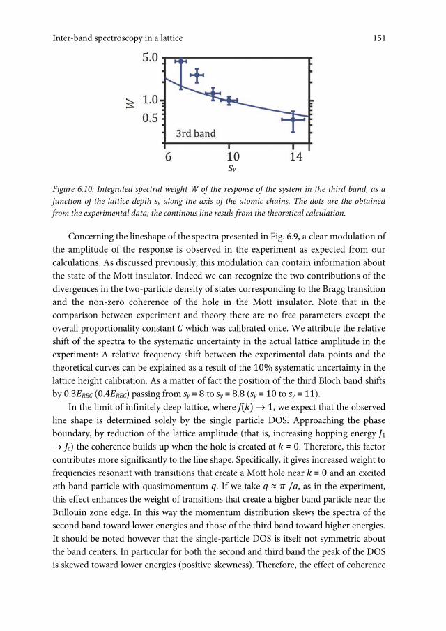
Interband spectroscopy in a lattice
151
Figure 6.10: Integrated spectral weight W of the response of the system in the third band, as a function of the lattice depth sy along the axis of the atomic chains. The dots are the obtained from the experimental data; the continous line resuls from the theoretical calculation.
Concerning the lineshape of the spectra presented in Fig. 6.9, a clear modulation of the amplitude of the response is observed in the experiment as expected from our calculations. As discussed previously, this modulation can contain information about the state of the Mott insulator. Indeed we can recognize the two contributions of the divergences in the two-particle density of states corresponding to the Bragg transition and the non-zero coherence of the hole in the Mott insulator. Note that in the comparison between experiment and theory there are no free parameters except the overall proportionality constant C which was calibrated once. We attribute the relative shift of the spectra to the systematic uncertainty in the actual lattice amplitude in the experiment: A relative frequency shift between the experimental data points and the theoretical curves can be explained as a result of the 10% systematic uncertainty in the lattice height calibration. As a matter of fact the position of the third Bloch band shifts by 0.3EREC (0.4EREC) passing from sy = 8 to sy = 8.8 (sy = 10 to sy = 11).
In the limit of infinitely deep lattice, where f(k) 1, we expect that the observed line shape is determined solely by the single particle DOS. Approaching the phase boundary, by reduction of the lattice amplitude (that is, increasing hopping energy J1 Jc) the coherence builds up when the hole is created at k = 0. Therefore, this factor contributes more significantly to the line shape. Specifically, it gives increased weight to frequencies resonant with transitions that create a Mott hole near k = 0 and an excited nth band particle with quasimomentum q. If we take q ≈ π /a, as in the experiment, this effect enhances the weight of transitions that create a higher band particle near the Brillouin zone edge. In this way the momentum distribution skews the spectra of the second band toward lower energies and those of the third band toward higher energies. It should be noted however that the single-particle DOS is itself not symmetric about the band centers. In particular for both the second and third band the peak of the DOS is skewed toward lower energies (positive skewness). Therefore, the effect of coherence
151Inter-band spectroscopy in a lattice

Nicole Fabbri
152
in the Mott insulator is to increase the skewness of the second band and decrease it in the third band spectra.
6.2 Conclusions
In conclusion, we have measured the response of two different periodic systems probing the inter-band excitations induced by inelastic light scattering. In the first experiment, we explore the response of a weakly-interacting three-dimensional condensate loaded in a 1D optical lattice. Changing the relative angle of the Bragg beams, we investigate excitations created both at the center and at the edge of the Brillouin zone. The results are in good agreement with mean-field Bogoliubov calculations. These inter-band measurements have been used as a reference to reveal the properties of a strongly correlated system, such as one-dimensional Mott insulating gases, that we investigated in a second experiment. In contrast to the case of a 3D BEC loaded in a 1D optical lattice, the spectra of these Mott states exhibit broad resonances in energy. The use of a band-mapping technique after applying the Bragg pulse allows us to identify these resonances with transitions towards the different energy bands induced by the optical lattice. We also give direct experimental evidence that the momentum distribution of Mott states spreads over the entire first Brillouin zone. This property enables us to reconstruct the dispersion relation of the high energy bands using a Bragg excitation at a fixed momentum transfer. Finally, the amplitude of the response of the inhomogeneous Mott insulating state in high-energy bands exhibits peculiar structures within a single excited band. The comparison with a model based on strong-coupling mean-field analysis has revealed the role of the Van Hove singularities in light scattering experiment with cold atoms. In addition, the asymmetry of the spectra has shown the effect of the quasi-hole excitation produced in the many-body ground-state of Mott insulator.
Nicole Fabbri152
Outlook and prospects
This thesis has been aimed at characterizing strongly correlated quantum systems in one dimension. We have approached this problem by realizing one dimensional ultracold gases trapped in optical lattices, and investigating them via inelastic light scattering.
The great interest that one dimensional systems have attracted in the last decades is related to the special role played by interactions in reduced dimensionality, that produces features drastically different from `normal' physics of three dimensional interacting systems. This has driven an enormous amount of experimental research in different fields, from material science to chemistry, which has resulted in the reali-zation of a large variety of 1D systems. However, most of the 1D compounds that have been studied or synthesized are in some sense complicated materials, where many different phenomena occur at once. Some agreement between the theoretical studies and the experimental observations can be reached but many open questions still remain. In particular, for most of these realizations, it is not straightforward how to quantitatively relate the specific microscopic properties with the general descrip-tion in terms of the Luttinger liquid universality class, which would predict the re-sponse of the system to weak perturbations and its correlation functions.
To overcome these complications, it would be a great opportunity to have other reference systems in which some degree of simplification occurs. Ultracold atoms in optical lattices can play this role. They offer almost total control over the lattice char-acteristics and over the fundamental physical parameters that govern the systems, such as the interaction strength. Thus, a strict relation between experiment and theo-retical description is possible. As a major advantage, the microscopic properties of the lattice gas (e.g., particle mass, density, scattering length) can be directly related to the Luttinger parameter which describes the universal collective behaviour of all the 1D systems. In addition, it is a virtually perfect rendering of the Hubbard type models. Then, one can add the other ingredients which make the picture more com-plicated (e.g., disorder) in a controlled way. This is in line with the original idea pro-posed by R. 193 [193] and later demonstrated by S. Lloyd [194] to realize a quantum simulator of models describing many particle quantum systems that are beyond the reach of any classical computer. Despite some experiments [195, 196] demonstrating
Nicole Fabbri, Bragg spectroscopy of quantum gases: Exploring physics in one dimension isBN 978-88-6655-220-8 (print) isBN 978-88-6655-221-5 (online) © 2012 Firenze University Press

Nicole Fabbri
154
few qubit quantum computers as a proof of principle, large scale quantum computers look not to be getting close, due to scalability hardly attainable. Instead, lattice gases provide full scale quantum simulators, which are already a specialized type of quan-tum computer, precisely aimed at simulating condensed matter models [149, 197].
In this context, it is crucial to better characterize the strongly correlated quantum phases that Bose gases realize in one dimension. This thesis has been intended to add new elements for the comprehension of it. As a probe technique, we used mainly ine-lastic light scattering (Bragg spectroscopy). As is commonly performed in solid state physics, the use of such a probe allowed us to gain important information about the atomic many body state, by investigating its response in the linear regime to an exci-tation at nonzero momentum. In this regime, Bragg spectroscopy gave us access to the dynamical structure factor �������and the one particle spectral func-tion����� ���of the system.
In a first experiment, we studied the coherence properties of an array of 1D Bose gases. We defined and measured via Bragg spectroscopy an effective coherence length as a mean property of the whole array. In defining it, we were supported by the re-sults of our simulations reproducing the response of the array, which showed the sys-tem to exhibit a single broad resonance dominated by thermal effects. In addition, we proposed and demonstrated time of flight absorption imaging to be a simple but powerful method to study the coherence properties in 1D systems with short coher-ence length. In this experiment, the measurement of the coherence length of the sys-tem also allowed an estimate of temperature, which is in general difficult to measure in a lattice gas. Only very recently, single site resolved detection has given access to the temperature of strongly correlated systems such as a Mott insulator, by measur-ing the variance on the lattice site occupation, which is related to temperature through the fluctuation dissipation theorem [164]. However, all the primary ther-mometers, i.e., the ones which employ intrinsic properties of the system for measur-ing temperature are affected by the approximations of the theory on which they are based. In exploring regimes for which no complete theory is at our disposal, one must have multiple primary thermometers based on different theoretical approximations, and then check for their consistency at low temperatures [149]. This can be the case, e.g., for 1D systems where both thermal effects and interactions play a relevant role and none of them can be neglected. On this prospect, our measurement provides one of these primary thermometers.
Then, a second experiment was dedicated to the study of 1D Bose gases im-mersed in a periodic lattice potential along their axis. For the values of the parameter γ, i.e., the ratio of interaction to kinetic energy experienced by 1D gases (� � 0.� �0.8), the system was well described by a Bose Hubbard Hamiltonian. By progressively increasing the lattice depth, the interaction induced transition from a superfluid state to an inhomogeneous Mott insulator state was investigated. The complexity of such
Nicole Fabbri154

Outlook and prospects
155
correlated quantum phases appears in the dynamical structure factor we measured via Bragg spectroscopy. From that, we identified the threshold value of the interac-tion strength above which the first Mott insulating lobe appears, surrounded by a su-perfluid. In addition, we characterized both the phases below and above this quan-tum critical point. This allowed the identification of the experimental signatures of strong atomic correlations and their link to the dynamical properties of the many body states. This point underlined the interest of using Bragg spectroscopy as a tool to probe low energy excitations in correlated quantum atomic phases.
Finally, the study was extended to inter band spectroscopy in a periodic lattice. This consisted of removing a particle from the many body ground state of the system and promoting it to a high energy band, where it is almost free since its energy is much larger than the typical ground state energy. A preparatory experiment was conducted on a Bose Einstein condensate in the presence of a 1D optical lattice, well captured by a mean field Bogoliubov picture. The measurements demonstrated the possibility to populate excitations in the higher energy bands of a periodic system, identified thanks to comparison with the Bogoliubov bands, which showed a good agreement. A band mapping measurement confirmed this identification, allowing the measurement of the momentum of the excited particles at different energy. This sys-tem was also used as a reference for more correlated situations. Indeed, in the last ex-periment, we performed inter band spectroscopy of a one dimensional Mott insula-tor. The band mapping of this system allowed us to reconstruct the dispersion rela-tion of the high energy bands of the system. In addition, the detailed analysis of the response of the system to excitation in the third band gave us information on the co-herence of the hole created in the many body ground state of the Mott insulator (thus, its one particle correlations).
At the end of this work, we can identify three main lines of research which would continue and extend it.
The current focus is in developing the study of more and more strongly interact-ing 1D Bose gases, to finally venture into the Tonks Girardeau regime, characterized by an interaction strength γ ∼ 1, corresponding to a Luttinger parameter � ∼ 1. In this regime, interparticle repulsive interactions become so strong to mimic the Pauli Exclusion Principle applicable to fermions. In this context, Bragg spectroscopy could be an excellent method for measuring the dynamical structure factor of this system. Several theoretical works have calculated the dynamical structure factor of 1D Bose gases both at zero temperature [171, 172, 170] and at finite temperature [198], as well as its one particle spectral function [199], but an experimental measurement is still missing. In order to realize this system, three possible strategies for increasing inter-actions are feasible. One can raise the scattering length by exploiting Feshbach reso-nances [41, 42]. However, the main problem of this approach is that the life time of the condensate strongly decreases due to three body losses, which rapidly grows
155Outlook and prospects
Nicole Fabbri
156
when the scattering length becomes large [200]. Another possibility is increasing the effective mass of the particles putting the 1D gas in a 1D optical lattice along its axis as in [34], though, in this case the filling factor � should be smaller than unity. Oth-erwise if doubly occupied sites would be present, as in our case, the direct corre-spondence to the Tonks Girardeau gas would be lost and the system would rather en-ter a Mott insulating phase (see [32]). As a third possibility, interactions can be en-hanced, compared to kinetic energy, by reducing the density �� as in [33]. In practice, this can be achieved, for example, by superimposing a blue detuned beam on the magnetic and lattice confinement to reduce the trapping frequencies. With an oppor-tune beam configuration, one can increase either the radial size of the whole cloud, in order to produce a larger number of 1D gases, or the axial size, in order to obtain more uniform 1D gases. This third realization of strongly interacting 1D gases im-plies a great advantage when investigating via Bragg spectroscopy. As a matter of fact, the lower the density, the lower is the Fermi wavevector �� � 2��� and the Fermi energy �� � �������2��. Thus, fixing the momentum imparted via Bragg scattering and decreasing the density, one can explore regions of the spectrum closer and closer to 2kF, where the peculiarity of the 1D systems is revealed. Indeed, gapped particle hole excitations are created for � � � � �� , corresponding to removal of a particle well below the Fermi surface and promoting it above this threshold, whereas at � � 2�� , i.e., at the border of the Fermi surface umklapp particle-hole excitations with vanishing energy can be created.
In the case that the 1D gases are immersed in a periodic potential along their axis, sufficiently strong interactions (γ ∼ 1) would open the way to additional fascinating prospects, allowing one to explore with ultracold gases beyond Hubbard type physics. In the current work we explored the effect of a periodic potential on 1D gases with relatively strong interaction, but still characterized by values of the dimensionless in-teraction strength γ ∼ 1, and the physics of the system was well captured by the Bose Hubbard model, predicting a quantum phase transition from superfluid to Mott in-sulator for deep enough lattices. Increasing the interactions would allows us to ap-proach the sine Gordon transition which brings a superfluid Luttinger liquid to a Mott insulator for arbitrarily weak amplitudes of the periodic potential [56]. This transition has been observed very recently via amplitude modulation spectroscopy [201], which implies a strong perturbation (of the order of 25% – 45% of the lattice amplitude). However, the linear response of the system, addressable with a weakly perturbing probe such as Bragg scattering, still needs to be investigated.
Another interesting line of research is the study of the interplay of disorder and interactions. The time of flight method we have proposed for studying phase fluctuat-ing 1D Bose gases could have an interesting application in measuring the coherence properties of strongly interacting disordered systems. This could help to reveal the role of thermal phase fluctuations in the nature of the superconductor insulator tran-
Nicole Fabbri156
Outlook and prospects
157
sition, which is an intriguing and still unclear theme [153, 154]. In this case, the re-markable control offered by ultracold atoms in an optical lattice would be a major advantage, allowing one to tackle the problem by realizing the 1D gases first, and then adding disorder in a controlled way. This really would be an example of a quan-tum simulator as Feynman first envisaged.
157Outlook and prospects

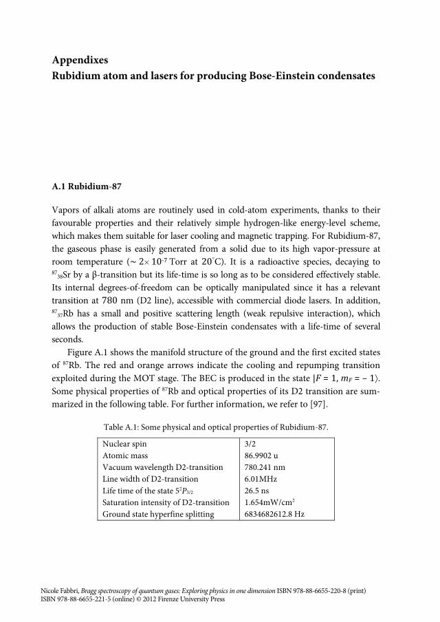
Appendixes Rubidium atom and lasers for producing Bose-Einstein condensates
A.1 Rubidium-87
Vapors of alkali atoms are routinely used in cold-atom experiments, thanks to their favourable properties and their relatively simple hydrogen-like energy-level scheme, which makes them suitable for laser cooling and magnetic trapping. For Rubidium-87, the gaseous phase is easily generated from a solid due to its high vapor-pressure at room temperature (∼ 2H 10‐7 Torr at 20BC). It is a radioactive species, decaying to 87
38Sr by a β-transition but its life-time is so long as to be considered effectively stable. Its internal degrees-of-freedom can be optically manipulated since it has a relevant transition at 780 nm (D2 line), accessible with commercial diode lasers. In addition, 87
37Rb has a small and positive scattering length (weak repulsive interaction), which allows the production of stable Bose-Einstein condensates with a life-time of several seconds.
Figure A.1 shows the manifold structure of the ground and the first excited states of 87Rb. The red and orange arrows indicate the cooling and repumping transition exploited during the MOT stage. The BEC is produced in the state |F = 1, mF = – 1. Some physical properties of 87Rb and optical properties of its D2 transition are sum-marized in the following table. For further information, we refer to [97].
Table A.1: Some physical and optical properties of Rubidium-87.
Nuclear spin Atomic mass Vacuum wavelength D2-transition Line width of D2-transition Life time of the state 52P3/2 Saturation intensity of D2-transition Ground state hyperfine splitting
3/286.9902 u 780.241 nm 6.01MHz 26.5 ns 1.654mW/cm2 6834682612.8 Hz
Nicole Fabbri, Bragg spectroscopy of quantum gases: Exploring physics in one dimension isBN 978-88-6655-220-8 (print) isBN 978-88-6655-221-5 (online) © 2012 Firenze University Press
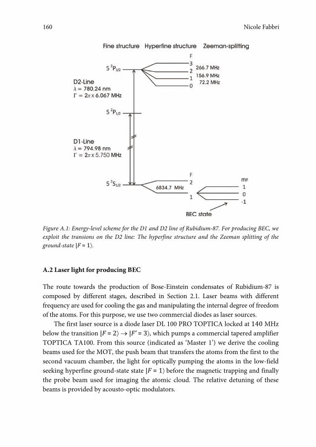
Nicole Fabbri
160
Figure A.1: Energy-level scheme for the D1 and D2 line of Rubidium-87. For producing BEC, we exploit the transions on the D2 line: The hyperfine structure and the Zeeman splitting of the ground-state |F = 1.
A.2 Laser light for producing BEC
The route towards the production of Bose-Einstein condensates of Rubidium-87 is composed by different stages, described in Section 2.1. Laser beams with different frequency are used for cooling the gas and manipulating the internal degree of freedom of the atoms. For this purpose, we use two commercial diodes as laser sources.
The first laser source is a diode laser DL 100 PRO TOPTICA locked at 140 MHz below the transition |F = 2 |F’ = 3, which pumps a commercial tapered amplifier TOPTICA TA100. From this source (indicated as ‘Master 1’) we derive the cooling beams used for the MOT, the push beam that transfers the atoms from the first to the second vacuum chamber, the light for optically pumping the atoms in the low-field seeking hyperfine ground-state state |F = 1 before the magnetic trapping and finally the probe beam used for imaging the atomic cloud. The relative detuning of these beams is provided by acousto-optic modulators.
Nicole Fabbri160

Outlook and prospects
161
Figure A.2: Laser light used in the experiment. All the necessary laser beams originate from two laser sources (“Master 1” and “Master Repumper”) by adding small detunings. The beams de-rived from Master 1 are represented in red; those derived from Master Repumper are in orange. “MOT cooling” and “MOT repumping” denote the transitions used together for laser cooling the atomic gas during both the two magneto-optical trapping stages. “Push” beam drives the atoms from the first vacuum chamber, where the first MOT stage occurs, to the second one, where we perform all the other stages for producing BEC and manipulating it in the experiments. “Optical Pumping” is used to transfer the atoms to the hyperfine sublevel |F = 1, mF = –1 that is mag-netically trappable. Absorption imaging of the atom is preceded by a “Pre-pumping” pulse that induce the atoms to decay into the |F = 2, mF = –2 hyperfine state; the images are recorded on the “Probe” transition.
The second master laser is a commercial diode laser DFB TOPTICA (called ‘Mas-ter Repumper’) and it is used as a repumping light for the MOT and pre-pumping before the imaging procedure. Figure A.2 summarizes the different laser-light frequen-cies used in the experiment and their detuning to the transitions between the hyperfine levels of Rubidium-87.
161Appendixes

Acknowledgements
My first thanks are to Chiara Fort, my PhD advisor. During these years, she has been always available sharing her wide and precious experience. Her dedication to re-search has been a true model for me. I am also indebted to Prof. Massimo Inguscio, who offered me the opportunity of joining his research group and undertaking this stimulating project, and supported and motivated us with his guidance.
This work was accomplished thanks the fundamental contributions of Leonardo Fallani, who always projected optimism in the group and gave suggestions that were true time-savers in the lab; David Clément, who was a reference-point for me for his ability in understanding both the fine details and the simple interpretation of physics problems; Michele Modugno, who provided us valuable theoretical input.
I would like to thank also the whole staff of LENS – the European Laboratory for Non-linear Spectroscopy, who created dynamical and supportive environment.
I also thank K. M. Richard van der Stam, Ehud Altman and Sebastian Huber for collaboration. I am indebted to Nir Davidson and co-workers for hospitality at the Weizmann Institute, where I found a very stimulating atmosphere; to Thierry Gia-marchi, Anna Minguzzi, Vitaly Golovach and Jean Sébastian Caux for fruitful discus-sions; to Peter Hannaford for having accurately read and referred this thesis.
Finally, I am deeply grateful to my parents Anna Rita and Roberto, to my sister Floriana, and to Carmine, who have always encouraged and helped me, along the whole way that brought me here.
Nicole Fabbri, Bragg spectroscopy of quantum gases: Exploring physics in one dimension isBN 978-88-6655-220-8 (print) isBN 978-88-6655-221-5 (online) © 2012 Firenze University Press


Bibliography
[1] A. Schwartz, M. Dressel, G. Grüner, V. Vescoli, L. Degiorgi, and T. Giamarchi, “On chain electrodynamics of metallic (TMTSF)2X salts: Observation of Tomonaga Luttinger liquid response”, Phys. Rev. B 58:1261 (1998).
[2] J. Hager, R. Matzdorf, J. He, R. Jin, D. Mandrus, M. A. Cazalilla, and E. W. Plummert, “Non Fermi liquid behavior in quasi one dimensional Li0.9Mo6O17”, Phys. Rev. Lett. 95:186402 (2005).
[3] F. Wang, J. V. Alvarez, J. W. Allen, S. K. Mo, J. He, R. Jin, D. Mandrus, and H. Höchst, “Quantum Critical Scaling in the Single Particle Spectrum of a Novel Anisotropic Metal”, Phys. Rev. Lett. 103:136401 (2009).
[4] T. Giamarchi, “Theoretical Framework for Quasi One Dimensional Systems”, Chem. Rev. 104 (11): 5037 (2004).
[5] A. G. Lebed (Editor), “The physics of organic superconductors and conductors”, Springer Series in Material Science, vol. 110 (Springer, 2008).
[6] D. A. Tennant and R. A. Cowley, “Measurement of the spin excitation continuum in one dimensional KCuF3 using neutron scattering”, Phys. Rev. B 52:13368 (1995).
[7] E. Dagotto, “Correlated electrons in high temperature superconductors”, Rev. Mod. Phys. 66:763 (1994).
[8] E. Dagotto and T. M. Rice, “Surprises on the way from one to two dimensional quantum magnets: The ladder materials” Science 271:5249 (1996).
[9] E. Dagotto, “Experiments on ladders reveal a complex interplay between a spin gapped normal state and superconductivity “, Rep. Prog. Phys. 62:1525 (1999).
[10] M. P. A. Fisher and L. I. Glazman, “Transport in a one dimensional Luttinger liquid”, in Proceeding of the NATO Advanced Study Institute on “Mesoscopic electron transport” ed. by L. L. Sohn, L. Kowenhoven, G. Schön (Kluwer Academic Publishers, Dordrecht, 1997).
[11] O. M. Auslaender, A. Yacoby, R. de Picciotto, K. W. Baldwin, L. N. Pfeiffer, and K. W. West, “Tunneling spectroscopy of the elementary excitations in a one dimensional wire”, Science 295: 825-828 (2002).
[12] R. Fazio and H. van der Zant, “Quantum phase transitions and vortex dynamics in superconducting networks”, Phys. Rep. 355:235 (2001).
[13] X. G. Wen, “Topological orders and edge excitations in fractional quantum Hall states”, Adv. Phys. 44:405 (1995).
[14] M. S. Dresselhaus, G. Dresselhaus, and P. C. Eklund, “Science of fullerenes and carbon nanotubes” (Academic Press, San Diego, 1995).
Nicole Fabbri, Bragg spectroscopy of quantum gases: Exploring physics in one dimension isBN 978-88-6655-220-8 (print) isBN 978-88-6655-221-5 (online) © 2012 Firenze University Press

Nicole Fabbri
166
[15] H. Ishii, H. Kataura, H. Shiozawa, H. Yoshioka, H. Otsubo, Y. Takayama, T. Miyahara, S. Suzuki, Y. Achiba, M. Nakatake, T. Narimura, M. Higashiguchi, K. Shimada, H. Namatame, M. Taniguchi, “Direct observation of Tomonaga Luttinger liquid state in car-bon nanotubes at low temperatures”, Nature (London) 426:540 (2003).
[16] M. H. Anderson, J. R. Ensher, M. R. Matthews, C. E. Wieman, and E. A. Cornell, “Obser-vation of Bose Einstein condensation in a dilute atomic vapor”, Science 269(0):198 (1995).
[17] K. B. Davis, M. O. Mewes, M. A. Joffe, M. R. Andrews, and W. Ketterle, “Evaporative cooling of sodium atoms”, Phys. Rev. Lett. 74:5202 (1995).
[18] M. B. Dahan, E. Peik, J. Reichel, Y. Castin, and C. Salomon, “Bloch oscillations of atoms in an optical potential”, Phys. Rev. Lett. 76:4508 (1996).
[19] P. J. Martin, B. G. Oldaker, A. H. Miklich, and D. E. Pritchard, “Bragg scattering of atoms from a standing light wave”, Phys. Rev. Lett. 60:515 (1988).
[20] D. M. Giltner, R. W. McGowan, and S. A. Lee, “Theoretical and experimental study of the Bragg scattering of atoms from a standing light wave”, Phys. Rev. A. 52:3966 (1995).
[21] D. M. Giltner, R. W. McGowan, and S. A. Lee, “Atom interferometer based on Bragg scat-tering from standing light waves”, Phys. Rev. Lett. 75:2638 (1995).
[22] E. M. Rasel, M. K. Oberthaler, H. Batelaan, J. Schmiedmayer, and A. Zeilinger, “Atom wave interferometry with diffraction gratings of light”, Phys. Rev. Lett. 75:2633 (1995).
[23] M. K. Oberthaler, R. Abfalterer, S. Bernet, J. Schmiedmayer, and A. Zeilinger, “Atom waves in crystals of light”, Phys. Rev. Lett. 77:4980 (1996).
[24] M. G. Prentiss, “Bound by light”, Science 260:1078 (1993). [25] M. Kasevich and S. Chu, “Laser cooling below a photon recoil with three level atoms”,
Phys. Rev. Lett. 69:1741 (1992). [26] J. Reichel, F. Bardou, M. Ben Dahan, E. Peik, S. Rand, C. Salomon, and C. Cohen
Tannoudji, “Raman cooling of Cesium below 3 nK: New approach inspired by Lévy flight statistics”, Phys. Rev. Lett. 75:4575 (1995).
[27] B. P. Anderson and M. A. Kasevich, “Macroscopic Quantum Interference from Atomic Tunnel Arrays”, Science 282:1686 (1998).
[28] S. Burger, F. S. Cataliotti, C. Fort, F. Minardi, M. Inguscio, M. L. Chiofalo, and M. P. Tosi, “Superfluid and dissipative dynamics of a Bose Einstein condensate in a periodic optical potential”, Phys. Rev. Lett. 86:4447 (2001).
[29] L. De Sarlo, L. Fallani, J. E. Lye, M. Modugno, R. Saers, C. Fort, and M. Inguscio, “Unsta-ble regimes for a Bose Einstein condensate in an optical lattice”, Phys. Rev. A 72:013603 (2005).
[30] F. S. Cataliotti, S. Burger, C. Fort, P. Maddaloni, F. Minardi, A. Trombettoni, A. Smerzi, and M. Inguscio, “Josephson Junction Arrays with Bose Einstein Condensates”, Science 293:293 (2001).
[31] M. Greiner, O. Mandel, T. Esslinger, T. W. Hänsch, and I. Bloch, “Quantum phase transi-tion from a superfluid to a Mott insulator in a gas of ultracold atoms”, Nature 415:39 (2002).
[32] T. Stöferle, H. Moritz, C. Schori, M. Köhl, and T. Esslinger, “Transition from a strongly interacting 1D superfluid to a Mott insulator”, Phys. Rev. Lett. 92:130403 (2004).
[33] T. Kinoshita, T. Wenger and D. Weiss, “Observation of a one dimensional Tonks Girardeau gas”, Science 305:1125 (2004).
Nicole Fabbri166
Bibliography
167
[34] B. Paredes, A. Widera, V. Murg, O. Mandel, S. Fölling, J. I. Cirac, G. V. Shlyapnikov, T. W. Haensch, and I. Bloch, “Tonks Girardeau gas of ultracold atoms in an optical lattice”, Nature 429:277 (2004).
[35] L. Fallani, J. E. Lye, V. Guarrera, C. Fort, and M. Inguscio, “Ultracold atoms in a disor-dered crystal of light: Towards a Bose glass”, Phys. Rev. Lett. 98:130404 (2007).
[36] R. Jördens, N. Strohmaier, K. Günter, H. Moritz, and T. Esslinger, “A Mott insulator of fermionic atoms in an optical lattice”, Nature (London) 455:204 (2008).
[37] U. Schneider, L. Hackermüller, S. Will, T. Best, I. Bloch, T. A. Costi, R. W. Helmes, W. Rasch, and A. Rosch, “Metallic and Insulating Phases of Repulsively Interacting Fermions in a 3D Optical Lattice”, Science 322:1520 (2008).
[38] L. Pitaevskii and S. Stringari, “Bose Einstein condensation” (Clarendon Press, Oxford, 2003).
[39] E. H. Lieb and W. Liniger, “Exact analysis of an interacting Bose gas. I. The general solution and the ground state”, Phys. Rev. 130:1605 (1963).
[40] F. Gerbier, A. Widera, S. Flling, O. Mandel, T. Gericke, and I. Bloch, “Interference pattern and visibility of a Mott insulator”, Phys. Rev. A 72:053606 (2005).
[41] P. Courteille, R. Freeland, D. Heinzen, F. van Abeelen, and B. Verhaar, “Observation of a Feshbach resonance in cold atom scattering “, Phys. Rev. Lett. 81:69 (1998).
[42] S. Inouye, M. Andrews, J. Stenger, H. J. Miesner, S. Stamper Kurn, and W. Ketterle, “Observation of Feshbach resonances in a Bose Einstein condensate”, Nature 392:151 (1998)
[43] I. Bloch, J. Dalibard and W. Zwerger, “Many body physics with ultracold gases”, Rev. Mod. Phys. 80:885 (2008).
[44] D. Jaksch and P. Zoller, “The cold atom Hubbard toolbox”, Ann. Phys. (N.Y.) 315:52 (2005).
[45] G. K. Campbell, J. Mun, M. Boyd, P. Medley, A. E. Leanhardt, L. G. Marcassa, D. E. Pritchard, and W. Ketterle, “Imaging the Mott insulator shells by using atomic clock shifts”, Science 313:649-652 (2006).
[46] J. T. Stewart, J. P. Gaebler and D. S. Jin, “Using photoemission spectroscopy to probe a strongly interacting Fermi gas”, Nature 454:744 (2008).
[47] T.-L. Dao, A. Georges, J. Dalibard, C. Salomon, and I. Carusotto, “Measuring the one particle excitations of ultracold fermionic atoms by stimulated Raman spectroscopy”, Phys. Rev. Lett. 98:240402 (2007).
[48] S. B. Papp, J. M. Pino, R. J. Wild, S. Ronen, C. E. Wieman, D. S. Jin, and E. A. Cornell, “Bragg spectroscopy of a strongly interacting 85Rb Bose Einstein condensate”, Phys. Rev. Lett. 101:135301 (2008).
[49] G. Veeravalli, E. Kuhnle, P. Dyke, and C. J. Vale, “Bragg spectroscopy of a strongly interacting Fermi gas”, Phys. Rev. Lett. 101:250403 (2008).
[50] D. Clément, N. Fabbri, L. Fallani, C. Fort, and M. Inguscio, “Exploring correlated 1D Bose gases from the superfluid to the Mott insulator state by inelastic light scattering”, Phys. Rev. Lett. 102:155301 (2009).
[51] X. Du, S. Wan, E. Yesilada, C. Ryu, D. J. Heinzen, Z. Liang, and B. Wu, “Bragg spectros-copy of a superfluid Bose Hubbard gas”, New J. Phys. 12:083025 (2010).
167Bibliography
Nicole Fabbri
168
[52] P. T. Ernst, S. Götze, J. S. Krauser, K. Pyka, D. S. Lühmann, D. Pfannkuche, and K. Sengstock, “Probing superfluids in optical lattices by momentum resolved Bragg spectros-copy”, Nat. Phys. 5:1 (2009).
[53] G. D. Mahan, “Many body Physics” (Plenum, New York, 1981). [54] D. S. Petrov, G. V. Shlyapnikov and J. T. M. Walraven, “Regimes of quantum degeneracy
in trapped 1D gases”, Phys. Rev. Lett. 84:3745 (2000). [55] M. Krämer, L. Pitaevskii and S. Stringari, “Macroscopic dynamics of a trapped Bose Ein-
stein condensate in the presence of 1D and 2D optical lattices”, Phys. Rev. Lett. 88:180404 (2002).
[56] T. Giamarchi, “Quantum Physics in One Dimension” Oxford Science Publications (Ox-ford, 2004).
[57] M. A. Cazalilla, A. F. Ho, and T. Giamarchi, “Interacting Bose gases in quasi one dimen-sional optical lattices”, New J. Phys. 8:158 (2006).
[58] F. D. M. Haldane,”Effective harmonic fluid approach to low energy properties of one di-mensional quantum fluids”, Phys. Rev. Lett. 47:1840 (1981).
[59] H. J. Mikeska and H. Schmidt, “Phase transition without long range order in two dimen-sions”, J. Low Temp. Phys. 2:371 (1970).
[60] M. Klanjsek, H. Mayaffre, C. Berthier, M. Horvatić, B. Chiari, O. Piovesana, P. Bouillot, C. Kollath, E. Orignac, R. Citro, T. Giamarchi, “Controlling Luttinger liquid physics in spin ladders under a magnetic field”, Phys. Rev. Lett. 101:137207 (2008).
[61] M. Olshanii, “Atomic scattering in the presence of an external confinement and a gas of impenetrable bosons”, Phys. Rev. Lett. 81:938 (1998).
[62] M. A. Cazalilla, “Bosonizing one dimensional cold atomic gases” J. Phys. B: At. Mol. Opt. Phys. 37, S1 (2004).
[63] M. D. Girardeau, “Relationship between systems of impenetrable bosons and fermions in one dimesion”, J. Math. Phys. 1:516 (1960).
[64] D. S. Petrov, G. V. Shlyapnikov and J. T. M. Walraven, “Phase fluctuating 3D Bose Ein-stein condensates in elongated traps”, Phys. Rev. Lett. 87:050404 (2001).
[65] F. Gerbier, J. H. Thywissen, S. Richard, M. Hugbart, P. Bouyer, and A. Aspect, “Momen-tum distribution and correlation function of quasicondensates in elongated traps”, Phys. Rev. A 67:051602(R) (2003).
[66] J. Hubbard, “Electron correlation in narrow energy bands”, Proc. Roy. Soc. A276:238 (1963).
[67] M. P. A. Fisher, P. B.Weichman, G. Grinstein, and D. S. Fisher, “Boson localization and the superfluid insulator transition”, Phys. Rev. B 40:546 (1989).
[68] D. Jaksch, C. Bruder, J. I. Cirac, C. W. Gardiner, and P. Zoller, “Cold Bosonic Atoms in Optical Lattices”, Phys. Rev. Lett. 81:3108 (1998).
[69] S. Sachdev, “Quantum Phase Transitions” (Cambridge University Press, Cambridge, Eng-land, 1999).
[70] K. Sheshadri, H.R. Krishnamurthy, R. Pandit, and T. V. Ramakrishnan, “Superfluid and insulating phases in an interacting boson model: Mean field theory and the rpa”, Europhys. Lett. 22:257 (1993).
[71] J. K. Freericks and H. Monien, “Phase diagram of the Bose Hubbard model”, Europhys. Lett. 26:545 (1995).
Nicole Fabbri168

Bibliography
169
[72] D. van Oosten, P. van der Straten, and H. T. C. Stoof, “Quantum phases in an optical lattice”, Phys. Rev. A 63:053601 (2001).
[73] N. Elstner and H. Monien, “Dynamics and thermodynamics of the Bose Hubbard model”, Phys. Rev. B 59:12184 (1999).
[74] T. D. Kühner and H. Monien, “Phases of the one dimensional Bose Hubbard model”, Phys. Rev. B 58:R14741 (1998).
[75] S. Rapsch, U. Schollwöck and W. Zwerger, “Density matrix renormalization group for disordered bosons in one dimension”, Europhys. Lett. 46:559 (1999).
[76] M. Rigol, G. Batrouni, V. Rousseau, and R. Scalettar, “State diagrams for harmonically trapped bosons in optical lattices”, Phys. Rev. A 79:053605 (2009).
[77] C. Fort, M. Prevedelli, F. Minardi, F. S. Cataliotti, L. Ricci, G. M. Tino, and M. Inguscio, “Collective excitations of a 87Rb Bose condensate in the Thomas Fermi regime”, Europhys. Lett. 49:8 (2000).
[78] M. Fattori, “Esperimenti di interferometria spaziale e temporale con condensati atomici di Bose Einstein”, Diploma thesis, Università degli Studi di Firenze (2001).
[79] P. Maddaloni, “Experiments on macroscopic quantum coherence in Bose Einstein condensates”, PhD thesis, University of Padova (2003).
[80] J. Catani, “Interazione tra un'onda di materia coerente e un reticolo ottico”, Diploma thesis, Università degli Studi di Firenze (2003).
[81] L. De Sarlo, “Instabilità di un condensato di Bose Einstein in un reticolo ottico”, Diploma thesis, Università degli Studi di Firenze (2004).
[82] L. Fallani, “Bose Einstein Condensates in Optical Lattices”, PhD thesis, Università degli Studi di Firenze (2004).
[83] N. Fabbri, “Diagnostica Hanbury Brown e Twiss per bosoni ultrafreddi in reticoli ottici”, Diploma thesis, Università degli Studi di Firenze (2007).
[84] V. Guarrera, “Bose Einstein Condensates in Disordered Optical Potentials”, PhD thesis, Università degli Studi di Firenze (2007).
[85] C. Cohen Tannoudji, “Atomic motion in laser light”, in “Fundamental Systems in Quan-tum Optics” edited by J. Dalibard, J. M. Raimond, J. Zinn Justin (Les Houches, 1990) Les Houches, Session LIII, July 1990, ed. by Dalibard J. and Raimond J.M., (Elsevier, 1992).
[86] D. E. Pritchard, E. L. Raab, V. Bagnato, C. E. Wieman, and R. N. Watts,”Light traps using spontaneous forces”, Phys. Rev. Lett. 57:310 (1986).
[87] C. Monroe, E. Cornell, and C. Wieman, “Laser Manipulation of Atoms and Ions” in “Proceedings of the International School of Physics Enrico Fermi”, Course CXVIII, edited by E. Arimondo, W. D. Phillips, and F. Strumia (North Holland, Amsterdam, 1992), pp. 361:377.
[88] J. R. Ensher, “The first experiments with Bose Einstein condensation of 87Rb”, PhD Thesis, University of Colorado (1998).
[89] J. Dalibard and C. Cohen Tannoudji, “Laser cooling below the Doppler limit by polariza-tion gradients: simple theoretical models”, J. Opt. Soc. Am. B 6(11):2023 (1989).
[90] E. Majorana, “Atomi orientati in campo magnetico variabile”, Il Nuovo Cimento 9:43 (1932).
[91] W. Petrich, M. H. Anderson, J. R. Ensher, and E. A. Cornell, “Stable, tightly confining magnetic trap for evaporative cooling of neutral atoms”, Phys. Rev. Lett., 74:3352 (1995).
169Bibliography

Nicole Fabbri
170
[92] D. E. Pritchard, “Cooling neutral atoms in a magnetic trap for precision spectroscopy”, Phys. Rev. Lett. 51:1336 (1983).
[93] T. Bergeman, G. Erez, and H. Metcalf, “Magnetostatic trapping fields for neutral atoms”, Phys. Rev. A 35:1535 (1987).
[94] H. Metcalf and P. van der Straten, “Laser Cooling and Trapping”, Springer (New York, 1999).
[95] W. Ketterle and N. J. van Druten, “Evaporative cooling of atoms”, in “Advanced in atom-ic, molecular and optical physics” edited by B. Bederson and H. Walther, 37:181-236 (1996).
[96] G. Reinaudi, T. Lahaye, Z. Wang, and D. Gury Odelin, “Strong saturation absorption im-aging of dense clouds of ultracold atoms”, Opt. Lett. 32:3143 (2007).
[97] D. A. 97, “Rubidium-87 D Line Data”, available at “http://george.ph.utexas.edu/ d97/alkalidata” (2001).
[98] Yu. Kagan, E. L. Surkov, and G. V. Shlyapnikov, “Evolution of a Bose condensed gas un-der variations of the confining potential”, Phys. Rev. A 54:R1753 (1996).
[99] Y. Castin and R. Dum, “Bose Einstein condensates in time dependent trap”, Phys. Rev. Lett. 77:5315 (1996).
[100] W. Ketterle, S. Durfee, and D. M. Stamper Kurn, “Making, probing and understanding Bose Einstein condensates”, in “Bose Einstein condensation in atomic gases”, Proc. of the International School of Physics Enrico Fermi, edited by M. Inguscio, S. Stringari and C.E. Wieman (IOS Press, Amsterdam, 1999).
[101] R. Grimm, M. Weidemüller, and Y. Ovchinnikov, “Optical dipole traps for neutral at-oms”, Adv. At. Mol. Opt. Phys. 42:95 (2000).
[102] J. H. Denschlag, J. E. Simsarian, H. Häffner, C. McKenzie, A. Browaeys, D. Cho, K. Helmerson, S. L. Rolston, and W. D. Phillips, “A Bose Einstein condensate in an optical lattice”, J. Phys. B: At. Mol. Opt. Phys. 35:3095 (2002).
[103] S. Hofferberth, I. Lesanovsky, B. Fischer, T. Schumm, and J. Schmiedmayer, “Non equi-librium coherence dynamics in one dimensional Bose gases”, Nature 449:324 (2007).
[104] B. Laburthe Tolra, K. M. O'Hara, J. H. Huckans, W. D. Phillips, S. L. Rolston, and J. V. Porto, “Observation of reduced three body recombination in a correlated 1D degenerate Bose gas”, Phys. Rev. Lett. 92:190401 (2004).
[105] M. Modugno, private communication. [106] S. Dettmer, D. Hellweg, P. Ryytty, J. Arlt, W. Ertmer, K. Sengstock, D. Petrov, G.
Shlyapnikov, H. Kreutzmann, L. Santos, and M. Lewenstein, “Observation of phase fluctu-ations in elongated Bose Einstein condensates”, Phys. Rev. Lett. 87:160406 (2001).
[107] S. Richard, F. Gerbier, J. H. Thywissen, M. Hugbart, P. Bouyer, and A. Aspect, “Momen-tum Spectroscopy of 1D Phase Fluctuations in Bose Einstein Condensates”, Phys. Rev. Lett. 91:010405 (2003).
[108] J. Estève, J. B. Trebbia, T. Schumm, A. Aspect, C. I. Westbrook, and I. Bouchoule, “Ob-servations of density fluctuations in an elongated Bose gas: ideal gas and quasicondensate regimes” Phys. Rev. Lett. 96:130403 (2006).
[109] T. Kinoshita, T. Wenger, and D. S. Weiss, “A quantum Newton's cradle”, Nature 440:900 (2006).
Nicole Fabbri170
Bibliography
171
[110] C. Menotti and S. Stringari, “Collective oscillations of a one dimensional trapped Bose Einstein gas”, Phys. Rev. A 66:043610 (2002).
[111] H. Moritz, T. Stöferle, M. Köhl, and T. Esslinger, “Exciting collective oscillations in a trapped 1D gas”, Phys. Rev. Lett. 91:250402 (2003).
[112] W. Zwerger, “Mott Hubbard transition of cold atoms in optical lattices”, J. Opt. B: Quantum and Semiclassical Optics 5:S9 (2003).
[113] A. Damascelli, Z. Hussain, and Z. Shen, “Angle resolved photoemission studies of the cuprate superconductors”, Rev. Mod. Phys. 75:473 (2003).
[114] N. W. Ashcroft and N. D. Mermin, “Solid State Physics” (Saunders, 1976). [115] P. Nozieres and D. Pines, “The Theory of Quantum Liquids” (Addison Wesley, Reading,
1994). [116] E. Arimondo, H. Lew, and T. Oka, “Deflection of a Na Beam by Resonant Standing
Wave Radiation”, Phys. Rev. Lett. 43:753 (1979). [117] V. A. Grinchuk, E. F. Kuzin, M. L. Nagaeva, G. A. Ryabenko, A. P. Kazantsev, G. I.
Surdutovich, and V. P. Yakovlev, Phys. Lett. (Elsevier) 86A 136 (1981). [118] P. L. Gould, G. A. Rou, and D. E. Pritchard, “Diffraction of atoms by light: the near
resonant Kapitza Dirac effect”, Phys. Rev. Lett. 56:827 (1986). [119] J. Y. Courtois, G. Grynberg, B. Lounis, and P. Verkerk, “Recoil induced resonances in
Cesium: an atomic analog to the free electron laser”, Phys. Rev. Lett. 72:3017 (1994). [120] M. Kozuma, L. Deng, E. W. Hagley, J. Wen, R. Lutwak, K. Helmerson, S. L. Rolston, and
W. D. Phillips, “Coherent splitting of Bose Einstein condensed atoms with optically in-duced Bragg diffraction”, Phys. Rev. Lett. 82:871 (1999).
[121] J. Stenger, S. Inouye, A. P. Chikkatur, D. M. Stamper Kurn, D. E. Pritchard, and W. Ketterle, “Bragg spectroscopy of a Bose Einstein condensate”, Phys. Rev. Lett. 82:4569 (1999).
[122] R. Ozeri, N. Katz, J. Steinhauer, and N. Davidson, “Colloquium: Bulk Bogoliubov excitations in a Bose Einstein condensate”, Rev. Mod. Phys. 77:187 (2005).
[123] D. M. Stamper Kurn, A. P. Chikkatur, A. Görlitz, S. Inouye, S. Gupta, D. E. Pritchard, and W. Ketterle, “Excitation of Phonons in a Bose Einstein Condensate by Light Scatter-ing”, Phys. Rev. Lett. 83:2876 (1999).
[124] J. Steinhauer, R. Ozeri, N. Katz, and N. Davidson, “Excitation Spectrum of a Bose Einstein Condensate”, Phys. Rev. Lett. 88:120407 (2002).
[125] J. Steinhauer, N. Katz, R. Ozeri, N. Davidson, C. Tozzo, and F. Dalfovo, “Bragg Spectros-copy of the Multibranch Bogoliubov Spectrum of Elongated Bose Einstein Condensates”, Phys. Rev. Lett. 90:060404 (2003).
[126] S. R. Muniz, D. S. Naik, and C. Raman, “Bragg spectroscopy of vortex lattices in Bose Einstein condensates”, Phys. Rev. A 73:041605(R) (2006).
[127] See, for example, H. Müller, S. Chiow, Q. Long, S. Herrmann, and S. Chu, “Atom interferometry with up to 24 photon momentum transfer beam splitters”, Phys. Rev. Lett. 100:180405 (2008), and references therein.
[128] Y. Inada, M. Horikoshi, S. Nakajima, M. Kuwata Gonokami, M. Ueda, and T. Mukaiyama, “Critical temperature and condensate fraction of a fermion pair condensate”, Phys. Rev. Lett. 101:180406 (2008).
171Bibliography
Nicole Fabbri
172
[129] D. van Oosten, D. B. M. Dickerscheid, B. Farid, P. van der Straten, and H. T. C. Stoof, “Inelastic light scattering from a Mott insulator”, Phys. Rev. A 71:021601 (2005).
[130] A. M. Rey, P. B. Blakie, G. Pupillo, C. J. Williams, and C. W. Clark, “Bragg spectroscopy of ultracold atoms loaded in an optical lattice”, Phys. Rev. A 72:023407 (2005).
[131] G. Pupillo, A. M. Rey, and G. G. Batrouni, “Bragg spectroscopy of trapped one dimen-sional strongly interacting bosons in optical lattices: Probing the cake structure”, Phys. Rev. A 74:013601 (2006).
[132] N. Fabbri, D. Clément, L. Fallani, C. Fort, M. Modugno, K. M. R. van der Stam, and M. Inguscio, “Excitations of Bose Einstein condensates in a one dimensional periodic poten-tial”, Phys. Rev. A 79:043623 (2009).
[133] N. Fabbri, D. Clément, L. Fallani, C. Fort, and M. Inguscio, “Momentum resolved study of an array of 1D strongly phase fluctuating Bose gases”, Phys. Rev. A 83:031604(R) (2011).
[134] R. Kubo, Can. J. Phys. 34:1274 (1956); R. Kubo, J. Phys. Soc. Japan 12:570 (1957). [135] H. A. Kramers, Atti del Congr. Intern. Fisica, Como 2:545 (1927). See Collected Scien-
tific Papers, North Holland, Amsterdam. [136] R. Kronig, J. Opt. Soc. Am. 12:547 (1926). [137] A. Brunello, F. Dalfovo, L. Pitaevskii, S. Stringari, and F. Zambelli, “Momentum trans-
ferred to a trapped Bose Einstein condensate by stimulated light scattering”, Phys. Rev. A 64:063614 (2001).
[138] D. Clément, N. Fabbri, L. Fallani, C. Fort, and M. Inguscio, “Bragg spectroscopy of strongly correlated bosons in optical lattices”, J. Low Temp. Phys. 158:5-15 (2010).
[139] F. Zambelli, L. Pitaevskii, D. M. Stamper Kurn, and S. Stringari, “Dynamic structure fac-tor and momentum distribution of a trapped Bose gas” Phys. Rev. A 61:063608 (2000).
[140] Yu. B. Ovchinnikov, J. H. Müller, M. R. Doery, E. J. D. Vredenbregt, K. Helmerson, S. L. Rolston, and W. D. Phillips, “Diffraction of a released Bose Einstein condensate by a pulsed standing light wave”, Phys. Rev. Lett. 83:284 (1999).
[141] M. Greiner, I. Bloch, O. Mandel, T. W. Hänsch, and T. Esslinger, “Exploring phase co-herence in a 2D lattice of Bose Einstein condensates”, Phys. Rev. Lett. 87:160405 (2001).
[142] P. Pedri, L. Pitaevskii, S. Stringari, C. Fort, S. Burger, F. S. Cataliotti, P. Maddaloni, F. Minardi, and M. Inguscio, “Expansion of a coherent array of Bose Einstein condensates, Phys. Rev. Lett. 87:220401 (2001).
[143] L. Van Hove, “Correlations in space and time and Born approximation scattering in sys-tems of interacting particles”, Phys. Rev. 95:249-262 (1954).
[144] S. Michotte, L. Piraux, S. Dubois, F. Pailloux, G. Stenuit and J. Govaerts “Superconduct-ing properties of lead nanowires arrays”, PhysicA 377C, 267 (2002).
[145] D. Y. Vodolazov, F. M. Peeters, L. Piraux, S. Mátéfi Tempfli, and S. Michotte “Current Voltage characteristics of quasi one dimensional superconductors: An S shaped curve in the constant voltage regime”, Phys. Rev. Lett. 91:157001 (2003).
[146] A. Iucci, M. Zvonarev, and T. Giamarchi, private communication. [147] V. N. Golovach, A. Minguzzi, L. I. Glazman, “Dynamic response of one dimensional
bosons in a trap”, Phys. Rev. A 80:043611 (2009). [148] F. Gerbier, “Condensats de Bose Einstein dans un piège anisotrope”, Ann. Phys. Fr. 29:1
(2004).
Nicole Fabbri172

Bibliography
173
[149] D. C. McKay and B. DeMarco, “Cooling in strongly correlated optical lattices: prospects and challenges”, e print arXiv:1010.0198.
[150] H. B. Thacker, “Exact integrability in quantum field theory and statistical systems”, Rev. Mod. Phys. 53:253 (1981).
[151] M. Srednicki, “Chaos and quantum thermalization”, Phys. Rev. E 50:888 (1994). [152] M. Rigol, V. Dunjko, and M. Olshanii, “Thermalization and its mechanism for generic
isolated quantum systems “, Nature 452:854 (2008). [153] P. Phillips and D. Dalidovich, “The elusive Bose metal”, Science 302:243 (2003). [154] Y. Dubi, Y. Meir, and Y. Avishai, “Nature of the superconductor insulator transition in
disordered superconductors”, Nature 449:876 (2007). [155] D. Clément, P. Bouyer, A. Aspect, and L. Sanchez Palencia, “Density modulations in an
elongated Bose Einstein condensate released from a disordered potential”, Phys. Rev. A, 77:033631 (2008).
[156] Y. Chen, J. Hitchcock, D. Dries, M. Junker, C. Welford, and R. G. Hulet, “Phase coher-ence and superfluid insulator transition in a disordered Bose Einstein condensate”, Phys. Rev. A, 77:033632 (2008).
[157] S. Fölling, A. Widera, T. Müller, F. Gerbier, and I. Bloch, “Formation of spatial shell structure in the superfluid to Mott insulator transition”, Phys. Rev. Lett. 97:060403 (2006).
[158] I. B. Spielman, W. D. Phillips, and J. V. Porto, “Mott insulator transition in a two dimensional atomic Bose gas”, Phys. Rev. Lett. 98:080404 (2007).
[159] S. Fölling, F. Gerbier, A. Widera, O. Mandel, T. Gericke, and I. Bloch, “Spatial quantum noise interferometry in expanding ultracold atom clouds”, Nature 434:481 (2005).
[160] V. Guarrera, N. Fabbri, L. Fallani, C. Fort, K. M. R. van der Stam, and M. Inguscio, “Noise correlation spectroscopy of the broken order of a Mott insulating phase”, Phys. Rev. Lett. 100:250403 (2008).
[161] H. Lignier, A. Zenesini, D. Ciampini, O. Morsch, E. Arimondo, S. Montangero, G. Pupillo, and R. Fazio, “Trap modulation spectroscopy of the Mott insulator transition in optical lattices”, Phys. Rev. A 79:041601(R) (2009).
[162] G. G. Batrouni, V. Rousseau, R. Scalettar, M. Rigol, A. Muramatsu, P. Denteneer, and M. Troyer, “Mott domains of bosons confined on optical lattices”, Phys. Rev. Lett. 89:117203 (2002).
[163] N. Gemelke, X. Zhang, C. L. Hung, C. Chin, “In situ observation of incompressible Mott insulating domains in ultracold atomic gases”, Nature 460:995 (2009).
[164] J. F. Sherson, C. Weitenberg, M. Endres, M. Cheneau, I. Bloch, and S. Kuhr, “Single atom resolved fluorescence imaging of an atomic Mott insulator”, Nature 467:68 (2010).
[165] C. Kollath, A. Iucci, T. Giamarchi, W. Hofstetter, and U. Schollwöck, “Spectroscopy of ultracold atoms by periodic lattice modulations”, Phys. Rev. Lett. 97:050402 (2006).
[166] G. G. Batrouni, F. F. Assaad, R. T. Scalettar, and P. J. H. Denteneer, “Dynamic response of trapped ultracold bosons on optical lattices”, Phys. Rev. A 72:0216901(R) (2005).
[167] S. D. Huber, E. Altman, H. Büchler, and G. Blatter, “Dynamical properties of ultracold bosons in an optical lattice”, Phys. Rev. B 75:085106 (2007).
[168] C. Menotti and N. Trivedi, “Spectral weight redistribution in strongly correlated bosons in optical lattices”, Phys. Rev. B 77:235120 (2008).
173Bibliography

Nicole Fabbri
174
[169] E. H. Lieb and W. Liniger, “Exact analysis of an interacting Bose gas. II. The excitation spectrum”, Phys. Rev. 130:1616 (1963).
[170] J. S. Caux and P. Calabrese, “Dynamical density density correlations in the one dimen-sional Bose gas”, Phys. Rev. A 74:031605(R) (2006).
[171] J. Brand and A. Yu. Cherny, “Dynamic structure factor of the one dimensional Bose gas near the Tonks Girardeau limit”, Phys. Rev. A 72:033619 (2005).
[172] A. Yu. Cherny and J. Brand, “Polarizability and dynamic structure factor of the one di-mensional Bose gas near the Tonks Girardeau limit at finite temperatures”, Phys. Rev. A 73:023612 (2006).
[173] Y. Kagan, N. V. Prokof'ev, and B. V. Svistunov, “Quasicondensation in a two dimen-sional interacting Bose gas”, Phys. Rev. A 61:045601 (2000).
[174] H. P. Büchler, V. B. Geshkenbein, and G. Blatter, “Superfluidity versus Bloch oscillations in confined atomic gases”, Phys. Rev. Lett. 87:100403 (2001).
[175] A. F. Ho, M. A. Cazalilla, and T. Giamarchi, “Deconfinement in a 2D optical lattice of coupled 1D boson systems”, Phys. Rev. Lett. 92:130405 (2004).
[176] K. Sengupta and N. Dupuis, “Mott insulator to superfluid transition in the Bose Hub-bard model: A strong coupling approach”, Phys. Rev. A 71:033629 (2005).
[177] S. Konabe, T. Nikuni, and M. Nakamura, “Laser probing of the single particle energy gap of a Bose gas in an optical lattice in the Mott insulator phase”, Phys. Rev. A 73:033621 (2006).
[178] Y. Ohashi, M. Kitaura, and H. Matsumoto, “Itinerant localized dual character of a strongly correlated superfluid Bose gas in an optical lattice”, Phys. Rev. A 73:033617 (2006).
[179] S. D. Huber, B. Theiler, E. Altman, and G. Blatter, “Amplitude Mode in the Quantum Phase Model”, Phys. Rev. Lett. 100:050404 (2008).
[180] U. Bissbort, Y. Li, S. Götze, J. Heinze, J. S. Krauser, M. Weinberg, C. Becker, K. Sengstock, and W. Hofstetter, “Detecting the Amplitude Mode of Strongly Interacting Lat-tice Bosons by Bragg Scattering', arXiv:1010.2205v1 (2010).
[181] K. Winkler, G. Thalhammer, F. Lang, R. Grimm, J. H. Denschlag, A. J. Daley, A. Kanti-an, H. P. Bchler, and P. Zoller, “Repulsively bound atom pairs in an optical lattice”, Nature 441:853 (2006).
[182] K. Berg Sörensen and K. Mölmer, “Bose Einstein condensates in spatially periodic po-tentials”, Phys. Rev. A 58:1480 (1998).
[183] B. Wu and Q. Niu, “Dynamical or Landau instability?”, Phys. Rev. Lett. 89:088901 (2002).
[184] C. Menotti, M. Krämer, L. Pitaevskii, and S. Stringari, “Dynamic structure factor of a Bose Einstein condensate in one dimensional optical lattice”, Phys. Rev. A 67:053609 (2003).
[185] M. Krämer, C. Menotti, L. Pitaevskii, S. Stringari, “Bose Einstein condensates in 1D op-tical lattices. Compressibility, Bloch bands and elementary excitations”, Eur. Phys. J. D 27:247 (2003).
[186] M. Modugno, C. Tozzo and F. Dalfovo, “Role of transverse excitations in the instability of Bose Einstein condensates moving in optical lattices”, Phys. Rev. A 70:043625 (2004).
Nicole Fabbri174
Bibliography
175
[187] D. Clément, N. Fabbri, L. Fallani, C. Fort, and M. Inguscio, “Multi band spectoscopy of inhomogeneous Mott insulator states of ultracold bosons”, New J. Phys. 11:1 (2009).
[188] N. Fabbri, S. D. Huber, D. Clément, L. Fallani, C. Fort, M. Inguscio, and E. Altman, “Quasiparticle dynamics in a Bose insulator probed by inter-band Bragg spectroscopy”, Phys. Rev. Lett. 109:055301 (2012).
[189] E. Altman, and A. Auerbach, “Oscillating superfluidity of bosons in optical lattices”, Phys. Rev. Lett. 89:250404 (2002).
[190] S. D. Huber, E. Altman, H. P. Büchler, and G. Blatter, “Dynamical properties of ultracold bosons in an optical lattice”, Phys. Rev. B 75:085106 (2007).
[191] T. Müller, Simon Fölling, A. Widera, and I. Bloch, “State preparation and dynamics of ultracold atoms in higher lattice orbitals”, Phys. Rev. Lett. 99:200405 (2007).
[192] S. Huber, private communication. [193] R. P. 193, “Simulating Physics with Computers”, Int. J. Theor. Phys. 21:467 (1982). [194] S. Lloyd, “Universal Quantum Simulators”, Science 273:1073 (1996). [195] S. Somaroo, C. H. Tseng, T. F. Havel, R. Laflamme, and D. G. Cory, “Quantum simula-
tions on a quantum computer”, Phys. Rev. Lett. 82:5381 (1999). [196] D. Leibfried, B. DeMarco, V. Meyer, M. Rowe, A. Ben Kish, J. Britton, W. M. Itano, B.
Jelenkovič, C. Langer, T. Rosenband, and D. J. Wineland, “Trapped ion quantum simula-tor: Experimental application to nonlinear interferometers”, Phys. Rev. Lett. 89:247901 (2002).
[197] M. Greiner and S. Fölling,”Optical lattices”, Nature 453:736 (2008). [198] A. Yu. Cherny and J. Brand, “Dynamic and static density density correlations in the one
dimensional Bose gas: Exact results and approximations”, Phys. Rev. A 79:043607 (2009). [199] J. S. Caux, P. Calabrese, and N. A. Slavnov, “One particle dynamical correlations in the
one dimensional Bose gas”, J. Stat. Mech. P01008 (2007). [200] P. O. Fedichev, M. W. Reynolds, and G. V. Shlyapnikov, “Three body recombination of
ultracold atoms to a weakly bounds level”, Phys. Rev. Lett. 77(14):2921 (1996). [201] E. Haller, R. Hart, M. J. Mark, J. G. Danzl, L. Reichsöllner, M. Gustavsson, M. Dalmonte,
G. Pupillo, and H. C. Nägerl, “Pinning quantum phase transition for a Luttinger liquid of strongly interacting bosons”, Nature 466:597 (2010).
175Bibliography

List of publications
Quasiparticle dynamics in a Bose insulator probed by inter-band Bragg spectroscopy N. Fabbri, S. D. Huber, D. Clément, L. Fallani, C. Fort, M. Inguscio, and E. Altman Physical Review Letters 109:055301 (2012) Momentum resolved study of an array of 1D strongly phase fluctuating Bose gases N. Fabbri, D. Clément, L. Fallani, C. Fort, and M. Inguscio Physical Review A 83:031604(R) (2011). Bragg spectroscopy of strongly correlated bosons in optical lattices D. Clément, N. Fabbri, L. Fallani, C. Fort, and M. Inguscio Journal of Low Temperature Physics 158:5 (2010).
Multi band spectroscopy of inhomogeneous gaseous Mott insulator states of ultra-cold bosons D. Clément, N. Fabbri, L. Fallani, C. Fort, and M. Inguscio New Journal of Physics 11:103030 (2009).
Excitations of Bose Einstein condensates in a one dimensional optical lattice N. Fabbri, D. Clément, L. Fallani, C. Fort, M. Modugno, K. M. R. van der Stam, and M. Inguscio, Physical Review A 79:043623 (2009).
Exploring correlated 1D Bose gases from the superfluid to the Mott insulator state by inelastic light scattering D. Clément, N. Fabbri, L. Fallani, C. Fort, and M. Inguscio, Physical Review Letters 102:155301 (2009).
Noise correlation spectroscopy of the broken order of a Mott Insulating phase V. Guarrera, N. Fabbri, L. Fallani, C. Fort, K. M. R. van der Stam, and M. Inguscio Physical Review Letters 100:250403 (2008).
Nicole Fabbri, Bragg spectroscopy of quantum gases: Exploring physics in one dimension isBN 978-88-6655-220-8 (print) isBN 978-88-6655-221-5 (online) © 2012 Firenze University Press
Nicole Fabbri
178
Bose Einstein condensation N. Fabbri and M. Fattori Quaderni di Storia della Fisica 16:221-254 (2010).
Probing correlations of gaseous microwires in optical lattices via inelastic light scat-tering N. Fabbri Nuovo Cimento C 34:75 (2010).
Inelastic light scattering to probe strongly correlated bosons in optical lattices C. Fort, L. Fallani, D. Clément, N. Fabbri, and M. Inguscio Journal of Physics: Conference Series, Proc. of the XXII International Conference on Atomic Physics – ICAP 2010, 264:012018 (2011).
Bragg spectroscopy of correlated gases L. Fallani, D. Clément, N. Fabbri, C. Fort, and M. Inguscio Laser Spectroscopy, Proc. of the XIX International Conference on Laser Spectroscopy – ICOLS 2009, p. 202-211, edited by H. Katori, H. Yoneda, K. Nakagawa, and F. Shi-mizu (World Scientific, 2010).
Analysis of the dynamical response of an array of one dimensional gases D. Clément, N. Fabbri, L. Fallani, C. Fort, and M. Inguscio in preparation.
Nicole Fabbri178

premio tesi di dottorato
year 2007Bracardi m., La Materia e lo Spirito. Mario Ridolfi nel paesaggio umbro Coppi e., Purines as Transmitter Molecules. Electrophysiological Studies on Purinergic Signalling in Different
Cell Systems mannini m., Molecular Magnetic Materials on Solid Surfaces Natali i., The Ur-Portrait. stephen Hero ed il processo di creazione artistica in a Portrait of the artist as a
Young man Petretto L., Imprenditore ed Università nello start-up di impresa. Ruoli e relazioni critiche
year 2008Bemporad F., Folding and Aggregation Studies in the Acylphosphatase-Like Family Buono a., Esercito, istituzioni, territorio. Alloggiamenti militari e «case Herme» nello Stato di Milano (secoli
XVI e XVII) Castenasi s., La finanza di progetto tra interesse pubblico e interessi privati Colica G., Use of Microorganisms in the Removal of Pollutants from the Wastewater Gabbiani C., Proteins as Possible Targets for Antitumor Metal Complexes: Biophysical Studies of their
Interactions
year 2009decorosi F., Studio di ceppi batterici per il biorisanamento di suoli contaminati da Cr(VI) di Carlo P., I Kalasha del Hindu Kush: ricerche linguistiche e antropologiche di Patti F., Finite-Size Effects in Stochastic Models of Population Dynamics: Applications to Biomedicine and
Biologyinzitari m., Determinants of Mobility Disability in Older Adults: Evidence from Population-Based
Epidemiologic Studies macrì F., Verso un nuovo diritto penale sessuale. Diritto vivente, diritto comparato e prospettive di riforma
della disciplina dei reati sessuali in Italia Pace r., Identità e diritti delle donne. Per una cittadinanza di genere nella formazione Vignolini s., Sub-Wavelength Probing and Modification of Complex Photonic Structures
year 2010Fedi m., «Tuo lumine». L’accademia dei Risvegliati e lo spettacolo a Pistoia tra Sei e Settecento Fondi m., Bioinformatics of genome evolution: from ancestral to modern metabolism. Phylogenomics and
comparative genomics to understand microbial evolution marino e., An Integrated Nonlinear Wind-Waves Model for Offshore Wind Turbines orsi V., Crisi e Rigenerazione nella valle dell’Alto Khabur (Siria). La produzione ceramica nel passaggio dal
Bronzo Antico al Bronzo Medio Polito C., Molecular imaging in Parkinson’s disease romano r., Smart Skin Envelope. Integrazione architettonica di tecnologie dinamiche e innovative per il
risparmio energetico
year 2011acciaioli s., Il trompe-l’œil letterario, ovvero il sorriso ironico nell’opera di Wilhelm HauffBernacchioni C., Sfingolipidi bioattivi e loro ruolo nell’azione biologica di fattori di crescita e citochineFabbri N., Bragg spectroscopy of quantum gases: Exploring physics in one dimensionGordillo Hervás r., La construcción religiosa de la Hélade imperial: El Panhelenionmugelli C., Indipendenza e professionalità del giudice in CinaPollastri s., Il ruolo di TAF12B e UVR3 nel ciclo circadiano dei vegetalisalizzoni e., Paesaggi Protetti. Laboratori di sperimentazione per il paesaggio costiero euro-mediterraneo


