Preoperative Planning Software for Corrective Osteotomy in Cubitus Varus and Cubitus Valgus João Tiago Pião Martins Thesis to obtain the Master of Science Degree in Biomedical Engineering Supervisor: M.D. Manuel de Azevedo Gomes Cassiano Neves Co-supervisor: Professor Joaquim Armando Pires Jorge Examination Committee Chairperson: Professor João Miguel Raposo Sanches Supervisor: M.D. Manuel de Azevedo Gomes Cassiano Neves Members of the Committee: Professor João Orlando Marques Gameiro Folgado November 2016
Transcript
Preoperative Planning Software for Corrective Osteotomy
in Cubitus Varus and Cubitus Valgus
João Tiago Pião Martins
Thesis to obtain the Master of Science Degree in
Biomedical Engineering
Supervisor: M.D. Manuel de Azevedo Gomes Cassiano Neves
Co-supervisor: Professor Joaquim Armando Pires Jorge
Examination Committee
Chairperson: Professor João Miguel Raposo Sanches
Supervisor: M.D. Manuel de Azevedo Gomes Cassiano Neves
Members of the Committee: Professor João Orlando Marques Gameiro Folgado
November 2016
i
RESUMO
A fratura supracondilar do úmero é a lesão do cotovelo mais comum em crianças e corresponde à
principal causa de cubitus varus e valgus. Embora estas deformações sejam vistas maioritariamente
como um problema estético, alguns estudos demonstraram que a progressão das mesmas pode
desencadear problemas mais graves. Por essa razão, um eficiente método corretivo para este tipo de
deformações é bastante importante, sendo que o método mais comum é a osteotomia de cunha
fechada realizada ao nível da porção distal do úmero.
Usualmente o planeamento pré-operatório é feito através de duas radiografias obtidas a partir de
uma visão ântero-posterior e de uma visão lateral. O maior problema associado a este método 2D
passa pelo facto de este tipo de deformações serem, na verdade, tridimensionais, tornando assim
bastante difícil planear a correção total desta malformação a partir de apenas dois ângulos de visão.
Nesta tese foi desenvolvido um software de apoio ao planeamento pré-operatório de uma
osteotomia de cunha fechada com deslocamento medial para casos de cubitus varus e cubitus valgus.
A principal inovação deste trabalho passa pela metodologia utilizada para o planeamento desta cirurgia,
uma vez que recorre a uma combinação das radiografias usuais com um modelo 3D da porção distal
do úmero. Desta forma, para além de ser possível determinar os ângulos de correção necessários para
o planeamento da osteotomia, este software também consegue simular esta técnica cirúrgica e criar
desta forma o modelo 3D do úmero pós-operatório.
As avaliações e comentários feitos pelos ortopedistas durante os testes realizados foram bastante
positivos, demonstrando assim que o software apresentado constitui uma solução viável para o
planeamento da cirurgia corretiva para este tipo de deformações.
The past few months were a very enriching experience for me and definitely different from the rest of
my academic journey. During this period, I was able to fully embrace a project of my own, facing
problems and difficulties that I have never before encountered. It was an experience that had its good
and its bad moments, but without a doubt it changed me and let me grow as a human being. However,
none of this work would be possible if it was not the people that, in a way or another, helped me during
all the project, and are to those that I want to express my gratitude.
To begin with, I would like to thanks to my supervisor M.D. Manuel de Azevedo Gomes Cassiano
Neves for the guidance provided during this project, for all the patience and time dispended with me,
and also for the data that he provided, which was essential for the growth and development of this work.
I also want to thanks to my co-supervisor Professor Joaquim Armando Pires Jorge for the feedback
given during this project, which was definitely helpful for the improvement of the work being done.
I want to give a special thanks to Doctor Daniel Simões Lopes, who, even not official, was a true
supervisor to me, and who was very supportive and guided me throughout all the project. Without him,
this project would not have gone through.
An important aspect of this project, besides of the work that was done, was the bounds and new
friendships that were created during these months. For that reason, I want to thanks to all my colleagues
that share the same room with me during this period, André Duarte, Nuno Matias and Sara Pires, who
not only helped me when I needed but also made this journey a lot funnier. Thanks guys!
I would also like to thanks to all my family, who were all so supportive and who gave me so much
strength when I needed during all my academic journey. A special thanks to my mom and dad, who
always took care of me and were always there when I needed: thanks for all the love!
Throughout all the challenges that I have faced during this last years, there was a special person
who have always been by my side, someone who helped and supported me during the toughest times:
to my girlfriend Catarina, the biggest thanks of all, for never letting me give up and for never stop
believing in me.
Finally, is necessary to recognize that none of this work could have gone through without financial
support. Therefore, I would like to acknowledge that this project was financially supported by national
funds through the Portuguese Foundation for Science and Technology with references IT-MEDEX
PTDC/EEISII/6038/2014 and UID/CEC/50021/2013.
vi
vii
TABLE OF CONTENTS
RESUMO ................................................................................................................................................... i
PALAVRAS-CHAVE ..................................................................................................................................... i
ABSTRACT ................................................................................................................................................ iii
KEYWORDS .............................................................................................................................................. iii
ACKNOWLEDGMENTS .............................................................................................................................. v
TABLE OF CONTENTS .............................................................................................................................. vii
LIST OF FIGURES ....................................................................................................................................... x
LIST OF ABBREVIATIONS ....................................................................................................................... xvii
Figure 17 - Osteology of the arm and the scapula (image from (Netter 2006)) .................................... 19
Figure 18 - Structure of a long bone (image from (Blaus 2014))........................................................... 20
Figure 19 - Muscle attachements on the arm and scapula, both at an anterior and posterior view (image
from (Netter 2006) ................................................................................................................................. 21
Figure 20 -Geometric modelling pipeline used on this work for the creation of the surface mesh of the
Figure 32 - Representation of a CSG tree algorithm, where the nodes represent the Boolean operations
between different objects: the – represents difference, the ∩ intersection and the ∪ union (image from
(Wikipedia, the free encyclopedia: Constructive Solid Geometry 2016)) .............................................. 40
Figure 33 - Construction of a BSP tree for 3D space, without (A) and with (B) the intersection of planes
(image adapted from (Segura, Stine e Yang 2013)) ............................................................................. 41
Figure 34 - Representation of the splitting of a triangle when intercepted by a plane (image adapted from
(Segura, Stine e Yang 2013)) ................................................................................................................ 42
Figure 35 - Introduction panel of the application. .................................................................................. 45
Figure 36 - The general appearance of the 2D Panel. It is possible to divide the panel into three sections:
the AP View (A), the Lateral View (B) and the Rotation Commands (C). ............................................. 46
Figure 37 - Example of a line segment created on the anteroposterior radiograph: the user only marked
points A and B, which correspond to the beginning and the end of the line segment. ......................... 47
Figure 38 - Example of the calculation of the angle made between the line segments 𝐵𝐴 and 𝐶𝐷. .... 47
Figure 39 - Contrast stretching function used for changing the gray intensity values of the image. The
movement of the slider will lead to the movement of both a and b points. ........................................... 48
Figure 40 - Example of contrast enhancement using the function describe on both radiographs. ....... 49
Figure 41 - Settings menu of the 2D panel, where is possible to change the reference values for both
Baumman's and Humeortrochlear angle, and is possible to access the help menu. ............................ 49
Figure 42 - Help window that explains all the commands and buttons of the 2D Panel. ...................... 50
Figure 43 – Demonstration of the features of the 2D Panel: the expansion of the radiograph with the
double-left click command (A), the zoom in into the radiograph with the mouse scroll wheel (B), and the
translation of the radiograph using the right click of the mouse (C). ..................................................... 51
Figure 44 – Calculation of the Baumann’s angle from the anteroposterior radiograph: the line segments
𝐵𝐴 and 𝐶𝐷 correspond to the humeral shaft axis and the lateral condyle axis drawn by the user, while
xiii
the segment 𝐵𝐸 represents the line perpendicular to 𝐵𝐴; this way, the Baumann’s angle will correspond
to the angle made between the vectors 𝐵𝐸 and 𝐶𝐷. ............................................................................. 52
Figure 45 - Calculation of the corrective angle necessary to be applied on the sagittal plane by
comparison of the Bauman's angle determined from the radiographs of the deformed arm with the value
used as a reference to the normal Baumann's angle value. ................................................................. 53
Figure 46 - Description of the method used for calculate the corrective angle based on the example
presented: first, the humerotrochlear angle of the deformed arm is determined using the vector of the
humeral shaft axis (𝐵𝐴) and the condyle axis (𝐶𝐷); then, this corrective angle is determined by
comparing the angle calculated to the reference value set at the application. ..................................... 54
Figure 47 - Window used to calculate the internal rotation of the deformity. ........................................ 55
Figure 48 - Determination of the corrective rotation angle from the lines that were drawn: the surface
line and the forearm line. The referential on the left represents when the angle measured will represent
an internal rotation or an external rotation correction: the blue and orange vectors represent the forearm
line, while the 𝑥 axis represent the surface line. ................................................................................... 56
Figure 49 - General appearance of the 3D Panel. All the commands on this panel are initially disabled
until the three points that are asked to the user mark are created. ....................................................... 57
Figure 50 – Positioning of the distal cutting plane according with the 3D model of the humerus. ........ 58
Figure 51 - Example of the marking of the three points that are asked on the 3D model: the first point to
be marked is the medial epicondyle (A), then the trochlea (B), and finally the lateral epicondyle (C). . 58
Figure 52 - Functioning of the widget: the spheres ill translate the object along the correspondent axis,
while the axes will rotate the object around the axis itself. .................................................................... 59
Figure 53 - Instantiating the PC plane and final positioning of the osteotomy site: since this plane is
anchored to the DC plane, the translation will affect both planes and only the rotation around the z-axis
is allowed. .............................................................................................................................................. 60
Figure 54 -Window with the anteroposterior radiograph that opens by clicking on the butto "AP View". It
is asked to the user mark three points on the radiograph: the medial epicondyle, the trochlea and the
Figure 67 - Steps performed using the simulation of the osteotomy until the final postoperative look is
achieved: (A) correspond the bone after performing the intersect Boolean operation, (B) is the bone after
applying the lateral cut angle, (C) is after applying the cutting angle, (D) corresponds to the bone after
rotating it according with the internal rotation of the deformity, (E) corresponds to the bone after the
translation is applied, and finally (F) is the final appearance of the bone, with both distal and proximal
parts joined together. ............................................................................................................................. 70
xv
Figure 68 – Representation on the 3D scene of both distal screw (DS) and proximal screw (PS), as well
as the guide. .......................................................................................................................................... 71
Figure 69 - Help window of the 3D Panel. ............................................................................................. 72
Figure 70 - Photos of the subjects testing the 2D Panel to determine the values of the corrective angles.
Figure 71 - Photos of the subjects testing the 3D panel of the application. .......................................... 75
xvi
xvii
LIST OF ABBREVIATIONS
3D – Three Dimensional
2D – Two Dimensional
CAOS – Computer-Aided Orthopaedic Surgery
CT – Computed Tomography
PDE – Partial Differential Equation
CAD – Computer-Aided Design
CSG – Constructive Solid Geometry
BSP – Binary Space Partitioning
CORA – Centre of Rotation of Angulation
AP – Anteroposterior
DC – Distal Cutting
PC – Proximal Cutting
DS – Distal Screw
PS – Proximal Screw
xviii
1
1. INTRODUCTION
1.1. Problem Statement
In orthopaedics, a good preoperative planning can be the difference between a successful
correction of a deformation and consequent recover of the normal function of the bone, or a not so
successful surgery that will not re-establish the functionality and the mobility of that anatomical structure.
For that reason, in last years many new approaches and techniques have emerged in this area, and
one topic that is becoming with the time more relevant is the use of computational techniques to perform
the planning of these surgeries, which is referred as the Computer Aided Orthopaedic Surgery (CAOS)
(Joskowicz and Hazan 2016).
The CAOS technologies are not exactly new in the orthopaedics world, since they have been
around for more than 25 years; however, these continue to improve every year. One of the simplest
application for this type of technologies, but very important, is the preoperative planning using 3D bone
surface modelling. This type of approaches can translate into much more accurate and less invasive
surgical interventions, and also a more accurate and better planning of the surgery, which can lead to a
lesser radiation exposure to the patient (Schep, Broeders and Werken 2003); the surgeons can even
simulate the plan that was defined to understand if it needs to be adjusted or not. Therefore, the use of
technologies as the ones referred above can be a game changing factor to determine the success of a
surgery, especially when talking about orthopaedic corrective approaches, where there is a strong visual
component associated to the preoperative planning. Finally, the CAOS systems can also give the doctor
a previous knowledge of the anatomy of the bone and of the site where the surgery is being performed:
with this knowledge, some complications and some unexpected surprises that could occur during the
surgery can be prevented.
The application developed in this work can be inserted, in fact, into the universe of the CAOS
technologies. What is presented here is an application developed to support the preoperative planning
of the corrective osteotomy for cubitus varus and valgus deformations, in which the user has access to
a three dimensional model of the bone that can be used to simulate the surgery that was planned.
1.1.1. Cubitus Valgus and Cubitus Varus
One of the most important and most valued aspects in everyone’s life is their mobility, which gives
them the freedom to go wherever they want and to accomplish most of the tasks by themselves. In order
to achieve this freedom, the correct positioning of the superior and inferior members is very important,
since this will lead to a correct movement and function of these members.
Unfortunately, not everyone has healthy bones, and some suffer from deformities that affect both
the aspect and the function of these bones. In this work, we will focus our attention to the cubitus varus
and valgus deformations, which corresponds to angular deformities of the distal part of the humerus
(Babhulkar 2015).
2
Both varus and valgus deformities are characterized by an abnormal angle between two bones
(according to the coronal plane) thanks to a wrong positioning of the distal portion of the bone in relation
with the proximal portion of the other bone that the first is in touch with. The difference between these
two is the value of the angulation that exists between the distal and the proximal parts, which will lead
to the opposite anatomical look: in the case of the varus deformity, the angle variation will lead to an
approximation of distal bone to the middle line of the body, in the coronal plane; on the other hand, the
valgus deformity will cause the opposite effect, with an increase of the distance to the middle line
(Oestreich 1990).
In the case of both cubitus varus and valgus, the most affected angle corresponds to the carrying
angle of the elbow, which is the angle made, along the anteroposterior plane, between the humeral shaft
and the forearm when the arm is fully extended and supinated (Figure 1) (Benson, et al. 2010). This
angle values oscillate between 11.6±3.2 degrees in the case of the men and 16.7±2.6 for the women
(Van Roy, et al. 2005). There are many factors that can lead to the formation of these deformities, such
as trauma, disease or congenital anomalies that affect the distal part of the humerus (Joseph, et al.
2016). Among those, for the cubitus varus, the most common is the supracondylar fracture of the
humerus, thanks to an incorrect reduction of the bone or even from the loss of the one made (Morrissy
and Weinstein 2006) (reduction corresponds to the procedure to restore the fracture or alignment of the
bone). In the case of the cubitus varus, most of the cases result from a lateral condylar fracture of the
humerus (Joseph, et al. 2016). Some reports have also related these deformities with sex chromosomal
anomalies that affect the carrying angle, such as the Tuner’s Syndrome and the Klinefelter’s Syndrome,
where taller individuals are associated to a lower carrying angle (valgus) while the smaller individuals
show a higher carrying angle value (varus) (Benson, et al. 2010, Joseph, et al. 2016).
In most cases, both cubitus varus and valgus do not affect the normal function of the elbow and
the motion of the person, being mostly a cosmetic problem (Joseph, et al. 2016); and in some cases the
deformity is only noticeable after several months, since it only becomes visible after the full extension
Figure 1 – Normal (left), valgus (middle) and varus (right) carrying angle variations (image from (Neumann 2015))
3
of the elbow joint being restored (Morrissy and Weinstein 2006). However, both these deformities can
lead to more severe problems. In the case of the cubitus valgus, the continues progression of the lesion
can lead to the stretch of the ulnar nerve thus causing ulnar nerve palsy, which corresponds to the
compression and consequent injury of the ulnar nerve that causes the paralysis of the muscle that are
affected by this nerve and therefore, the loss of sensation and muscle strength of the hand (Guardia
2016). For the cubitus varus cases, the ulnar nerve palsy can also occur due to the continuous
compression and subluxation of the nerve (Joseph, et al. 2016), which results from a dislocation of the
olecranon fossa to the ulnar side of the distal humerus, as well as a movement of the triceps ulnarwards;
besides that, some studies have been associating an increase of the risk of fracture of the lateral
condyle, thanks to abnormal stresses resented at it, and in some cases difficulty at throwing due to the
varus angle variation of the carrying angle (Babhulkar 2015). Other reports showed a relation between
cubitus varus situation to posterolateral rotation instability, an internal rotation malalignment, pain and
dislocation of the radial head (Joseph, et al. 2016, Srivastava, et al. 2016).
Since the supracondylar fracture of the humerus, the main cause of these deformities, is a common
lesion in the children (nearly 3% of all the fractures), it makes sense that this age group is the one with
a higher prevalence of both cubitus varus and valgus. In fact, these type of fractures are very rare in
adults, which make these deformities rarer as well (Piggot, Graham and McCoy 1986, Bonczar, Rikli
and Ring n.d.).
Therefore, a correct treatment of both deformities can be very important to these children: not only
for improving their cosmetic aspect, but also to prevent any type of nerve damage and any kind of joint
instability, which are both caused by the long progression of these angular variations (Joseph, et al.
2016). However, not always the treatment is effective, and in some cases the patient is not happy with
the final result of the cosmetic appearance due to the prominence of the lateral condyle (Morrissy and
Weinstein 2006).
4
1.1.2. Current Surgical Techniques
The only way to treat both cubitus varus and valgus is through an osteotomy applied at the distal
portion of the humerus, and depending if the deformity is progressive or non-progressive, it may be
necessary more than one surgical intervention to solve it (Srivastava, et al. 2016). However, there are
many variations of this surgical approach that can be used to fixe these deformations, and all of them
have different configurations for the osteotomy, different fixation methods and different approaches to
the deformity (medial, anteromedial, lateral, posterior and posterolateral) (Tanwar, et al. 2014).
Choosing the type of osteotomy that is more suitable for each case is done according to several
indications that are well defined in the literature (Joseph, et al. 2016). Nowadays the three more common
types of osteotomies that are used for these cases are the Medial Opening Wedge Osteotomy with Bone
Graft, the Oblique Osteotomy and the Lateral Closing Wedge Osteotomy (Babhulkar 2015). However
many different approaches that result from these three have been emerging in order to minimize the
secondary effects and the negative aspects of theirs.
The most common, simple and safer technique among these is the Lateral Closing Wedge
Osteotomy with K-wire fixation (Figure 2), in which the osteotomy site is set above the olecranon fossa
and a wedge is cut from the distal portion of the humerus. The biggest problem associated to this
method, when not followed by a dislocation of the distal part of the bone, is the increase of the
prominence of the lateral condyle (in the case of cubitus varus) and of the prominence of the medial
epicondyle (for the cubitus valgus), as well as the creation of a secondary deformity. Another problem
associated to this type of osteotomy is the creation of a scar on the outer part of the elbow, which results
from the fact that is performed a lateral approach instead of a medial one. This approach also does not
seems to fix the hyperextension problem, which causes the ulnar nerve palsy, and also the internal
rotation of the deformity, that may lead to an increase of the instability of the elbow joint (Joseph, et al.
Figure 2 –Lateral Closing Wedge technique for both cubitus varus and valgus without (middle) and with (right) medial displacement of the distal part (image from (Joseph, et al. 2016))
5
2016). Since the place where the osteotomy is performed is more proximal than the malunited
metaphysis itself, this will make the fixation of the pins harder, and therefore will be harder to achieve a
solid fixation of the bones as well. Finally, the last issue associated with this approach is related with the
tightness of the medial soft tissue that is achieved postoperative, which creates a high varus moment
that may be the cause of recurrent deformation when the bone is not correctly fixed (El-Adl 2007).
In order to deal with the problems associated with this kind of osteotomy, many other approaches
and techniques have been emerging and been developed, and some of them will be described in the
following section.
The most similar approach to the previous one described and whose main goal is to minimize the
prominence of the lateral condyle and the medial epicondyle for cubitus varus and valgus, respectively,
is to perform a Lateral Closing Wedge Osteotomy with a medial displacement of the distal portion
resulting from the osteotomy (Figure 2) (Joseph, et al. 2016).
One way to deal with the prominence of the lateral condyle in the varus cases is to perform Lateral
Closing Wedge Osteotomy but with equal limbs (El-Adl 2007), a method that, besides being able to
resolve this issue, is not that harder to reproduce. As described at El-Adl (2007), the main idea of this
method is to draw the corrective angle into a triangle card with the same limbs length, which will be used
afterwards for marking the supracondylar area at the osteotomy site. After this, the osteotomy is
performed so that the medial cortex remains intact, and is closed very carefully in order to avoid its
fracture. Finally, the bones are fixated with two crossing Kirschner wires (or K-wires, correspond to a
pointed stainless steel wires used in orthopaedic surgery (Knipe and Morgan 2016)). The results
obtained at this study using this technique were pretty satisfactory, where the children presented similar
post operatory radiographies for both arms, as well as a similar cosmetic appearance, with almost none
prominence of the lateral condyle.
Another technique that has emerged as a response to resolve the complications that were
associated to the Lateral Closing Wedge Osteotomy was the Dome Osteotomy (Hahn, Choi and Kang
2009). In this approach, the osteotomy is made along a semicircle, with an approximately 3cm radius,
Figure 3 – The steps of the Lateral Closing Wedge Osteotomy with equal limbs, using as fixation method two crossing Kirschner wires (figure from (El-Adl 2007))
6
that is centred at a point situated 1cm distal from the olecranon. After the cut is made, the distal part
resulting from the osteotomy is rotated along the coronal plane until the corrective angle that was
previously determined is achieved, and then the bones are fixated using a combination between plates
and Kirshner wires. As described at Hahn, Choi and Kang (2009), this technique has demonstrated to
be a possible alternative to the one described previously, especially on adults, since it has demonstrated
to be an easier approach when comparing with others that are also alternatives to the simple lateral
closing wedge osteotomy, and does not seems to have any problems related with the creation of the an
ugly scar or the prominence of either the medial condyle and the medial epicondyle (Kumar, et al. 2014).
Although this technique seems to become much harder when is necessary to perform a correction of
the internal rotation of the deformity, it has been reported better results fixing the internal rotation issue
using the Dome Osteotomy than with other techniques (Kumar, et al. 2000). However, there have been
studies that showed a higher prevalence of postoperative problems using a dome osteotomy than with
a lateral closing wedge osteotomy, problems such infections, ulnar nerve palsy, loss of motion,
circulatory issues, among others.
Another approach that has been developed to overcome the disadvantages associated to the
lateral wedge osteotomy is the step cut osteotomy (Figure 5). As described at Bali, et al. (2011), the first
step is to mark the osteotomy site by drawing a line perpendicular to the lateral supracondylar ridge
within 1.5cm to 2cm proximal to the olecranon fossa. After that, another line is marked according to the
corrective angle that was previously determined, which will have the same length as the line that was
firstly draw. From those lines it is possible to determine the section of the bone that is necessary to cut
with the osteotomy, as well as any necessary portions of the bone that are necessary to be removed in
order to maintain the alignment of both distal and proximal portions and to avoid any lateral prominence.
Therefore, the main advantages of this method when comparing to the lateral cutting wedge is the ability
Figure 4 – Dome Ostetotomy technique: the semicircle of the osteotomy is marked on the humerus (A), and then the correction is made by rotating the distal part until the corrective angle value is achieved (B) (figure from (Kumar, et al. 2000))
7
to avoid any type of lateral prominence on the postoperative scenario and a lesser visible scar, and also
has lesser postoperative problems when comparing with the dome osteotomy described previously.
The Oblique Closing Wedge Osteotomy corresponds to a good alternative to the approaches that
were previously talked when dealing with adults. The main difference between performing a corrective
osteotomy on an adult or on a children is the fracture healing time and the tendency for stiffness for
each of them (Gong, et al. 2008). In the case of the children, they have high healing capacities, which
allow them to almost fully recover from the surgery and to union completely the distal and proximal
portion of the humerus really fast (within 3-6 weeks). On the other hand, in the case of the adults this
Figure 5 - Step Cut Osteotomy: first, the varus/valgus and the corrective angles angle are determined (a) and the corrective osteotomy site is determined (b); then, the step cut osteotomy is performed, with the remotion of any additional parts at the proximal portion to avoid any prominence (c); finally, the alignement is made after the osteotomy (figure from (Bali, et al. 2011))
Figure 6 - Oblique Closing Wedge Osteotomy: first the deformity angle is determined (A) and the osteotomy site is marked obliquely (B); then the osteotomy is performed and the distal portion is positioned in a way that the lateral aspect ends up with a continuous aspect (C); finally, the proximal portion is cutted in order to avoid any additional prominences (D) (figure from (Bali, et al. 2011))
8
recuperation period can be much longer, and in some cases it can even last 3 months before the bone
is fully united. One big advantage of the oblique osteotomy is the increase of the contact area between
the distal and proximal parts after the osteotomy, which will help with healing process of the bone. In
addition, this osteotomy also allows the fixation of the bones with lag screws, which are bigger and have
a greater holding capacity, leading thus to a much stable fixation, which also helps with the healing
process of the bone. In this Oblique approach, as expected, in the case of the cubitus varus deformity
the wedge is set in an oblique position with an angle that is equal to the correction angle that was
determined during the planning and with the vertex pointing to the proximal portion of the humerus. After
the cut, the distal part is repositioned so that there the lateral condyle as a continuous aspect, avoiding
thus any unwanted prominence. The proximal part of the osteotomy face is also cut in order to correct
any deformity that may result from the osteotomy. If necessary, any internal rotation of the deformity
can also be corrected by rotating the distal portion using the lateral cortex as a hinge (Gong, et al. 2008).
The described technique can be seen in Figure 6.
The last approach that is going to be discussed in this section is the Medial Opening Wedge
Osteotomy with Bone Graft. In this method, the correction of the deformity is based on the Illizarov
technique (Figure 7). The positioning of the hinge and of the osteotomy site will be determined from the
joint line and the centre of rotation of angulation (CORA). This way, the hinge for the mechanism will be
placed at the apex of the osteotomy line that was previously determined and whose pass thought the
CORA, and from which is possible the correction of the deformity. In order to fixate this mechanism, a
set of wires, rods and three rings (one distal and two proximal) are used: for the fixation of the distal
ring, a first wire is inserted from posterolateral face of the lateral condyle to the anterior cortex of the
medial condyle, at an inclination of around 6% to the joint line, and will be fixed at the distal ring; the
second wire will pass from the medial epicondyle to the anterior cortex of the lateral condyle, and will
be fixed as well at the distal ring; for the proximal rings, a wire is fixed anterolaterally. These three rings
are also connected to each other by three equidistant rods. Not only the insertion of these wires is made
using an image intensifier guidance, but also the osteotomy is made under this imaging method. The
osteotomy in this case is performed from the medial side (MM, et al. 2015, Piskin, et al. 2007). The main
Figure 7 – Correction of a cubitus varus deformity using the Illizarov method (figure from (Piskin, et al. 2007))
9
disadvantages associated to this method are the risk of causing any damage to the ulnar nerve due to
the lengthening and stretching that is made to it, as well as the instability that is associated to this
method (Babhulkar 2015).
In all the methods that were previously described, the preoperative planning of the surgery is made
based on radiographs acquired at an anteroposterior view and at a lateral view. The anteroposterior
view radiograph is obtained with the elbow fully extended and the forearm supinated, while the lateral
view one is obtained with a 90º elbow flexion and the palm and the forearm rested at a table (Park and
Kim 2009, Shetty n.d.). There are many ways to determine the corrective osteotomy angles that are
necessary to correct the deformity: in the case of the anteroposterior view, some reports use the carrying
angle of the elbow as a measurement of the deformity, while others seem to use the Baumann’s angle;
for the lateral view, the humerotrochlear angle is a good indicator if is necessary or not a correction of
the deformity along the sagittal plane.
The carrying angle of the elbow corresponds to the angle formed between the intersection of the
long axis of the humeral shaft (or simply the long axis of the arm) and the long axis of the forearm on
the anteroposterior view. The corrective angle may be determined by comparison of the carrying angle
of the arm with the deformity to the carrying angle of the opposite arm (when the radiographs of that
arm are also available) or to the standard values that are described at the literature for this angle, which
for the children is about 5º to cubitus valgus (Oestreich 1990). However, the mean values for the carrying
angle can range between a large set of values, and not only between different genders, as reported at
Park and Kim (2009).The value for this angle from which the corrective osteotomy becomes necessary
is not consensual to every orthopaedics, although these values are all within a certain range. For
Figure 8 - Preoperative planning using an anteroposterior view radiograph in order to determine the deformity angle.
10
example, at Tanwar, et al. (2014) any varus angle value above 10º was an indicative for the need of
perform a corrective osteotomy, while at Bali, et al. (2011) it was necessary at least a 20º deformation
to the surgery be considered as an option.
The Baumman’s angle, which is also determined within the anteroposterior view, is obtained by the
intersection of line that is perpendicular to the long axis of the humeral shaft with the line that is parallel
to the lateral condyle. The normal value for this angle is around 15º. Just like in the case of the carrying
angle, the correction angle can be determined by comparison of the Baumman’s angle of the arm without
deformity to the one deformed, when available the radiographs, or by comparison with the literature
value for this angle.
In the case of the humerotrochlear angle, this one is measured with the lateral view radiography
and is given by the intersection of the longitudinal line of the humeral shaft with the axis of the condyles.
Like the other angles, the correction angle can be given by comparison with the healthy arm of the
person or with the value for this angle that is described at the literature, which is around 40º.
Finally, the internal rotation of the deformity is also measured during the preoperative planning, but
it is not measured using the radiographs like the previous angles. In fact, there is not any simple or well
Figure 9 - Methods for calculating the Baumman's angle (left) and the Humerotrochlear angle (right), as well as the literature values for both of them (figure from (Medscape n.d.))
Figure 10 – Using Yamamoto method for determining the internal rotation of the deformity (figure from (Kim, Lee and Yoo 2005))
11
documented clinical method for the measure of this rotation angle. However, most of the studies seems
to follow the Yamamoto method (Yamamoto, et al. 1985) to determine the internal rotation deformity
(Figure 10). In this method, the patient is positioned slightly bend with the shoulder at maximum
extension and the elbow at a 90º flexion. While in this position, in normal subjects the angle made
between the horizontal line of the back and the axis of the forearm is approximately 0º. However, in
subjects with a cubitus varus/valgus deformation the same does not happens, where it is possible to
see an increase of the angle made between these two lines (Yamamoto, et al. 1985). Another simple
method to determine the rotation of the deformity is to have the patient laid down with the arm abducted,
the forearm flexed at 90º and the shoulder fully externally rotated: in normal subjects, the angle made
between the forearm and the table is 0º; on the other hand, for patients with either cubitus varus or
valgus the same does not occur, and the angle that is measured will correspond to the rotation that is
necessary to be applied.
12
1.2. Literature Review
One of the biggest flaws of the current corrective approaches for both cubitus varus and valgus is
related with the preoperative planning. Nowadays, this planning is made by using radiographs that are
acquired at an anteroposterior and lateral view. However, in the case of cubitus varus and valgus the
deformities are in fact three dimensional, which makes for any planning based on a 2D approach very
hard to fully correct the bone malformations based on only two different angles. As described at Omori,
et al. (2014), some previous studies revealed that the corrective osteotomy based on the 2D
preoperative planning would lead to a mean value of residual deformity on the distal humerus of around
5-8%.
For that reason, some research work is being done around this theme in order improve both the
preoperative planning and the corrective osteotomy surgery, achieving thus better postoperative results.
An area that seems to be in a great expansion around this subject is the planning of the corrective
osteotomy using 3D imaging techniques that use sets of Computed Tomography (CT) images from both
arms of the subjects in order to plan the corrective surgery and simulate the aspect of the arm on the
postoperative scene (S. Omori, T. Murase, et al. 2014, Oka, Murase, et al. 2011, Zhang, et al. 2011,
Bryunooghe 2015, Takeyasu, et al. 2011, Oka, Murase, et al. 2012, S. Omori, T. Murase, et al. 2015,
Tricot, Duy and Docquier 2012, Tricot, Duy and Docquier 2012).
A major advantage of an approach that uses a set of CT images of the distal humerus is the
possibility to create a specific osteotomy guide and plate for each patient, which can improve greatly the
Figure 11 –Steps of a preoperative planning using the 3D simulation software described: it is possible to see the surgical guide designed and the simulation of the final aspect of the bone on a postoperative scenario after the osteotomy (figure from (Oka, Murase, et al. 2011))
13
final results and appearance of the arm, and overall the accuracy of the corrective surgery. Many studies
have been done in the last years comparing the postoperative results obtained using a normal
preoperative planning from two 2D radiographs (anteroposterior and lateral view) and a planning that is
based on 3D imaging techniques.
A research group in Japan (Oka, Murase, et al. 2011) developed a 3D simulation software, using
C++, whose main purpose was to be used for the planning of corrective osteotomies for deformities like
cubitus varus and valgus. The idea of this simulation software was to perform, from the CT images, the
segmentation of the bones, creating thus the representative mesh models of the bone surface, and
plane the osteotomy from those. In the case of this report, the evaluation of the deformity was made by
comparison of both the healthy arm and the one with the deformity. This way, the two meshes obtained
from the segmentation process were superimposed, and the deformity was then determined and
described in terms of a rotation and a translation in relation to a certain axis. After the simulation was
done, custom guides and custom bone plates specific for each patient were made using this software
as well, which would be used during the surgery in order to replicate the results obtained during the 3D
simulation (Figure 11). Although in this study the methodology was only tested in cadaver bones, the
results were pretty satisfactory, where in all the cases the guide fitted really well at the bone, with no
visible gaps between the two, and the corrective osteotomy went as it was planned in the software.
The same group, describes at Takeyasu, et al. (2011) a comparative study between the
conventional planning approach that uses radiographs to this 3D preoperative planning for cases of
cubitus varus deformities resulting from supracondylar fracture of the humerus. In this study, the
measure of the angles necessary to fully plan the corrective osteotomy were determined by
superimposing the deformed arm with a mirror of the healthy one. This way, the lesion was quantified
Figure 12 - Evaluation of the deformity by sumperimposing the healthy and deformed arms. The deformity is avaliated in terms of the varus angulation (A), extension (B) and internal rotation (C) (figure from (S. Omori, T. Murase, et al. 2015))
14
in terms of the varus angulation, internal rotation and extension. With the results obtained they
concluded that the 3D evaluation was more accurate, especially in terms of the extension and internal
rotation of the deformation (Figure 12). Even more recently (2015), they reported another study whose
purpose was to test once again the accuracy of this three dimensional simulation software for correction
of cubitus varus deformations (Figure 13) (S. Omori, T. Murase, et al. 2015). The assessment of the
lesion was also made my superimposing the healthy and the deformed arms. In this case, in order to
evaluate the accuracy of this 3D approach, a postoperative CT scan was performed in order to obtain a
3D model of the bone after the osteotomy being performed, and then this model was superimposed to
the preoperative model that was obtained during the simulation. The results obtained were pretty good,
with a postoperative carrying angle of the arm with the lesion with a mean difference to the normal arm
of only 0.6%-0.7%.
At S. Omori, T. Murase, et al. (2014), another research group used the same software to perform
corrective osteotomies on cadavers at the distal humerus and radius. In this report, the results are also
Figure 13 - Preoperative simulation for correction of a cubitus varus deformity: the deformity is defined by superimposing the two arms and the cutting planes are placed on the model (A); then, the model is cut simulating the osteotomy (B), the distal portion is rotated so it gets in contact with the proximal part (C) and finally the distal part is moved in order to correct align both parts (D) (image from (S. Omori, T. Murase, et al. 2015))
Figure 14 - Simulation of the surgery using the patient specific guide designed: from A-D at an anteroposterior view, and from E-H the same procedure but viewed from a lateral view (image from (S. Omori, T. Murase, et al. 2015))
15
very promising, since both the guide and fixation plate fitted correctly on the bone, and the osteotomy
went according to the preoperative planning simulation.
Some research groups have been testing the performance of others 3D methodologies like the one
described previously in real cases of cubitus varus and valgus deformations. Pierre-Louis Docquier and
his team (Tricot, Duy and Docquier 2012)describe a new technique for the correction of distal humerus
malformations. Using a set of CT images, with the Mimics software it was made the 3D reconstruction
of the bone and the preoperative planning of the osteotomy. The patient-specific guide was made using
a printed 3D model of the distal humerus that was previously marked, and the fixation plate was also
premoulded using a printed model of the corrected bone (Figure 15). The results obtained were also
satisfactory, with a low error rate (1%-9%) between the correction obtained and the one planned.
A Chinese group (Zhang, et al. 2011) tested the accuracy of a different 3D approach for treatment
of cubitus varus deformation on teenagers (Figure 16). In this study, the three dimensional
reconstruction of the bone was made using the Mimics software, like it was made by Docquier, and then
the model was imported to the Imageware software, where all the preoperative planning was made. The
corrective osteotomy was planned by measuring both the carrying angle and the tilting angle from the
3D model, and the guide was printed using as material an acrylate resin after making the simulation.
For all the 18 patients, the corrective osteotomy was successful, with the radiographs showing little
anatomical difference between both arms.
These three dimension approaches besides providing a more accurate assessment of the cubitus
varus and valgus deformities, when comparing to the traditional radiographs planning, are also able to
decrease the duration of the corrective procedure and the complexity of the equipment needed thanks
to the patient-specific guides and plates that result from this novel planning. However, this three
dimensional methodology also has some disadvantages. One that is common to all the studies referred
Figure 15 – A simple patient-specific guide for corrective surgery on cubitus varus deformity. Here it is showed the guide being used on a 3D printed model of the humerus to simulate the use of the guide during a real surgery (image from (Tricot, Duy and Docquier 2012))
16
is the increase of radiation exposure to the patient, due to the CT-scanning that is necessary to perform,
in the majority of the cases, to both arms. This type of methodologies also have an increased cost
associated, which can be a problem for the patients. Most of the techniques described previously have
room for improvement: as an example, the one described at Tricot, Duy and Docquier (2012), where it
was only performed a simple closing wedged osteotomy with no distal movement correction due to the
limitations of the method that didn’t allow to measure the translation necessary to be applied.
Some attempts have been made in order to overcome these problems. As an example, the Osaka
University in Japan (Oka, Murase, et al. 2009) conducted a study to evaluate the accuracy of the
reconstructed three dimensional models obtained from multidetector computed tomography data. The
main purpose was to find the appropriate parameters of the CT scan that allowed a reduction of the
radiation exposure to the patient while maintaining the accuracy of the 3D models. In fact, with a lower
radiation dose CT (around one-thirtieth of the normal dose) they were able to achieve a model with the
same accuracy as the one reconstructed from a normal dose CT data. Although this study is an
important step in the right direction, and can be one key aspect to make these three dimensional
methodologies more viable, it only solves one problem of the ones referred previously, meaning that are
still many more that need to be assessed.
Figure 16 - Preoperative planning to create the custom made guide (image from (Zhang, et al. 2011))
17
1.3. Contribution of the Thesis
As described in the previous section, the current three dimensional softwares still have some
problems that need to be overcome.
In this work it was developed a software for preoperative planning of cubitus varus and valgus that
is based on a novel technique that can be described as a mixture between the conventional planning
that uses two radiographs (one at an anteroposterior view and another at a lateral view) and a three
dimensional planning methodology that uses a reconstruction of the bone with the deformity from a CT
data set. The planning of the corrective osteotomy is made by measuring both the Baumman’s angle
and the tilting (or humerotrochlear) angle on the two radiographs, like it is made when using the
conventional planning. However, the value of these angles will be extrapolated to the 3D model, where
it is possible to simulate the corrective osteotomy and see the final aspect of the bone. In addition, in
this software it is also possible to estimate the necessary translation that is necessary to be applied to
the distal portion in order to fully correct the deformity and maintain the CORA.
That being said, the main advantage of this approach when compared with the previous ones is the
reduction of radiation exposure to the patient, since it is not necessary a second CT scan to the healthy
arm, unlike the previous cases, because the planning of the corrective osteotomy is not made by
superimposing the 3D models of both arms. Another advantage of this software is the ability to fully plan
a closing wedge osteotomy with medial displacement of the distal portion of the osteotomy, since it is
possible to determine the translation that is necessary to apply, something that is not achievable by all
the three dimensional methodologies that were referred in the previous section.
18
19
2. OSTEOLOGY OF THE ARM
The skeleton of the arm corresponds to the humerus, which is a long bone that articulates
proximately with the scapula and distally with the ulna and the radius. This bone is constituted by the
diaphysis (or shaft), that corresponds to the midsection of the bone, and two extremities, which are
formed by the metaphysis and the epiphysis (Pina 1999, Netter 2006).
The shaft has a form similar to a triangular prism, with the proximal portion showing a more
cylindrical aspect, while the distal part is equilaterally triangular in its cross-section, and also has a
double isosceles triangles right above the elbow joint. The shaft has three faces (posterior, anterolateral
and anteromedial) and three borders (anterior, lateral and medial).
The anterolateral surface, situated between the anterior and lateral borders, has the deltoid tubercle
right above the middle of its surface, which is where the deltoid and brachialis muscles attaches too,
Figure 17 - Osteology of the arm and the scapula (image from (Netter 2006))
20
and it is very smooth in its upper portion, whose is covered by the deltoid muscle. At a more distal part
of this surface, below the deltoid tubercle, it is where the lateral fibres of brachialis are positioned.
The anteromedial surface, on the other hand, is situated between the anterior and medial borders.
The upper half of this surface that is right below the intertubercular sulcus is very smooth and does not
have any muscle attached to it, while the lower half is where the medial part of the brachialis muscle fits
in. This surface has a rough area, at the middle third of it, where the coracobrachialis is attached too,
and right above is where the nutrient foramen can be found. At the lowest portion of this surface it can
be found the medial supracondylar ridge, which is where the humeral head of pronator teres and the
medial intermuscular septum of the arm are attached to.
Finally, the posterior surface situates between the medial and lateral borders. Along this surface it
is possible to see the radial groove, which is a shallow groove where the radial nerve, its branches and
the profunda brachii vessels are inserted in, and which extends from the medial portion of the posterior
surface downwards and laterally to the lateral border. Below medial portion of the bone, there is a
triangular area that almost occupy the lower end of the bone and which is where the medial head of the
triceps is attached to. In the case of the lateral head of triceps, this muscle is attached to a rough ridge
that extends above the medial head attachment site.
The anterior border extends from the greater tubercle to the lower extremity of the bone. Its proximal
third is much roughed, since it is where the muscle are attached, and it forms the lateral lip of the
intertubecular sulcus. The area below this area is as well roughed and it delimits anteriorly the deltoid
tubercle. Lastly, the rest of the border is smooth and rounded.
In the case of the lateral border, at the lower end of the bone it becomes thicker and forms the lateral
supracondylar ridge. At its medial portion, this border has the deltoid tubercle and is also where the
Figure 18 - Structure of a long bone (image from (Blaus 2014))
21
radial groove passes through. Besides, it is to the lateral border that the lateral intermuscular septum is
attached to, which is more visible at the lower three-fifths of the arm.
At last, the medial border at the lower half of the shaft gives origin to the medial supracondylar ridge.
At the proximal third of this border there is a triangular area, whose lateral border will form the medial
lip of the intertubercular sulcus, and the medial border will extends to the anatomical neck, where it gets
roughed and with vascular apertures, creating thus an area for the attachment of the shoulders capsule.
At its middle third, this border is run by the radial groove, which passes obliquely from the posterior
surface towards the anterior surface.
Like it was mentioned previously, the humerus has two extremities: the proximal and the distal end.
The proximal end has four evident structures, which are the head, the anatomical neck and both the
greater and lesser tubercles, and it is connected to the shaft by the surgical neck.
The head has a spheroid form with a smooth articular surface, it is covered by hyaline cartilage, and
it articulates with the glenoid cavity of the scapula, although only with a certain portion since the size of
the head is bigger than the cavity itself. In the case of the anatomical neck, it is at the margins of the
head, and creates in fact a slightly constriction to it. The anatomical neck delimits the place of attachment
of the shoulder joint, with the exception at the intertubercular sulcus, since it is where the long tendon
of biceps passes through. For the lesser tubercle, it is situated anterior and beyond to the anatomical
neck, and its lateral edge will give origin to the medial border of the intertubercular sulcus (that situates
in fact between the lesser and the greater tubercle). Both the subscapularis muscle and the transverse
ligament of the shoulder joint are attached to the lesser tubercle. Finally, the greater tubercle, which
corresponds to the lateral part of the proximal end, is the larger area of this extremity. At its
Figure 19 - Muscle attachements on the arm and scapula, both at an anterior and posterior view (image from (Netter 2006)
22
posterosuperior surface is possible to distinguish three different impressions: the uppermost, which is
where the supraspinatus is attached too, the middle one, for the infraspinatus, and the lowest, in the
case of the teres minor. The lateral surface of the greater tubercle has many vascular foramina
(openings for the vascular vessels), and it is covered by the deltoid.
As mentioned previously, the intertubercular sulcus is situated between the two tubercles, and it is
where the long tendon of biceps, the synovial sheath and an ascending branch of the anterior circumflex
humeral artery are lodged on. In its lateral lip it is where the tendon of the pectoralis major situated, on
the medial lip the tendon of the teres major, and, finally, on the floor lip the tendon of the latissimus
dorsi. The muscles itself are also present at the lips for the respective tendons.
The last part of the humerus that remains to be described is the distal end. The distal end is a
condyle with a wide and flat aspect, and it is constituted by both articular and non-articular portions. The
articular portions correspond to the capitulum and the trochlea. The capitulum is a half sphere projection
that articulates with the head of the radius, and it is in contact with the inferior face of the radius when
the elbow is fully extended and with the anterior surface when the elbow is flexed. In the case of the
trochlea, it is separated on its lateral side from the capitulum by a groove and its medial side extends to
the rest of the bone. The trochlea articulates with the trochlear notch of the ulna: when the elbow is
extended it is in contact with the ulna the inferior and posterior surfaces; otherwise, when it is flexed,
the posterior surface of the trochlea gets exposed.
In terms of the non-articular portions, they are the medial and lateral epicondyles, the olecranon,
the coronoid and radial fossae. The medial epicondyle corresponds to a medial projection at the condyle,
which is easily visible during the flexion of the elbow. On its posterior surface there is a shallow groove
from where the ulnar nerve runs by; on the other hand, at its posterior surface it is where the forearm
flexors are attached. The lateral epicondyle is situated at the lateral border of the condyle, and its end
part gives origin to the lateral supracondylar ridge. Its anterior and lateral surfaces correspond to an
area where the flexors of the forearm are attached too.
About the three fossae that were referred previously, the olecranon fossa is situated above the
trochlea, on the posterior surface of the condyle, and it is where the olecranon of the ulna fits when the
elbow is fully extended. The coronoid fossa it is situated at the anterior surface of the condyle, also
above the trochlea, and it lodge the anterior margin of the coronoid process of the ulna when the elbow
is flexed. Finally, the radial fossa stays above the capitulum, on the lateral side of the condyle, and it is
where the margin of the head of the radius fits in during the full flexion of the elbow.
23
3. GEOMETRIC MODELING
One of the most important feature of the software that was developed in the current work is the
ability to simulate the corrective osteotomy performed at the distal portion of the humerus, giving the
user an idea of the postoperative appearance of the bone. For that reason, the creation of a three
dimensional model that provides a very good approximation of the real bone is an essential step to
achieve a reliable simulation of the osteotomy.
In this work, the creation of a 3D model from the CT data was done by using a well described
geometric modelling pipeline, as described in Figure 20 (Lopes 2006, Lopes 2013, Ribeiro, et al. 2009).
The first step is to perform the image segmentation of the CT images in order to identify and extract the
desired tissues. From the segmentation information, a surface mesh of the model is created using the
marching cubes algorithm, and then the obtained mesh is smoothed to improve its geometry. Finally, a
decimation operation will also be applied to the mesh to remove the redundant nodes and surfaces that
do not affect the overall geometry of the mesh.
Each of these steps were achieved by using different software: in the case of the image
segmentation and mesh generation, this was done by using the ITK-SNAP (version 3.4)(ITK-SNAP
2016), while both smoothing and decimation were achieved with the Paraview (version 4.3.1) (ParaView
2016). Finally, it was necessary a third software, the Blender (version 2.75) (Blender 2016), to convert
the final mesh into a format that could be used on the application developed.
CT Data • Medical Images (*.DCM)
ImageSegmentation
• ITK-SNAP (*.MHA)
MeshAdjustments
• Paraview (*.PLY - ASCII)
File Convertion
• Blender(*.OBJ)
Figure 20 -Geometric modelling pipeline used on this work for the creation of the surface mesh of the distal humerus
24
3.1. Image Segmentation
Creating a three dimensional representation of bone from a set of two dimensional images is not
an easy task. To do so, it is necessary to extract meaningful information and to identify different regions
from these images. Image segmentation can be defined as the clustering of the pixels of an image
according to some criteria, like colour, intensity or texture, in order to partitioning the image into well-
defined, homogeneous and with simple boundaries regions. Therefore, the image segmentation is an
essential aspect of any three dimensional reconstruction pipeline, since this process of regions
separation is necessary to be possible to reconstruct only the desired objects of an image (Dass,
Priyanka and Devi 2012).
Although it seems to be a pretty simple process, the image segmentation is not in fact trivial at all.
Each image has different characteristics that need to be taken in consideration, making it difficult to find
a single approach that can be applied to all the different types of images. For that reason, there are in
fact many different image segmentation techniques that can be used according with the image that
needs to be segmented: none of these techniques are good for every different type of images and not
all of them are equally good for a certain type of image (Pal and Pal 1993). Even the choice of the right
approach for each image is a difficult task.
It is possible to split the segmentation methods into two categories: the ones that detect
discontinuities, which are the methods that perform the partition of the image based on abrupt changes
in intensity, and the ones that detect similarities, which correspond to the algorithms that split the image
into different regions according with the similarity of the pixels around a certain criteria. All of these
algorithms are based on three segmentation approaches, which are the thresholding, the edge-based
methods and the region-based methods (Biomathematics & Statistics Scotland n.d.).
The methods based on thresholding are the simplest and the most common ones, and they are
very effective when dealing with images with dark backgrounds and light objects. In these thresholding
approaches a multilevel image is converted into a binary image according to a certain threshold, which
is very useful for separating a region, like the background of an image, from the rest of the objects. To
do so, a pixel is classified as belonging within a region according with equation 1: if the intensity 𝑓(𝑖, 𝑗)
Figure 21 - Example of a segmentation of a CT image, where there are two different regions: the red area correspond to one region, while the rest of the image will correspond to the other region, the background.
25
of the pixel at the coordinates (i,j) is higher than the threshold previously set (T), then it will be classified
as part of the region; otherwise, the pixel will be classified as belonging to the other region.
𝑓(𝑖, 𝑗) ≥ 𝑇 (1)
In the majority of the cases, this threshold is selected manually, although there are methods that
can determine the threshold necessary to apply in order to perform a correct segmentation of the image.
Depending on the type of thresholding value that is applied, it is possible to distinguish two methods of
thresholding: a Global and a Local thresholding (Dass, Priyanka and Devi 2012, Zhang, Qu and Wang
2006). In the case of the Global thresholding, the same threshold is applied to all pixels of the image. In
the case of the Local thresholding, there are multiple threshold values that are applied to different
regions of the image, depending on the illumination distribution.
Depending on the number of different regions that are achieved, these thresholding segmentation
methods can be classified into bi-level or multilevel thresholding. In the first case, the image is
segmented into two different regions; on the multilevel thresholding, the image is partition into many
sub-regions, which is useful when there are many different objects in the same image (Pal and Pal
1993). The biggest disadvantage of the thresholding segmentation methods is the fact that these
methods do not take in consideration any spatial characteristics of the image (Dass, Priyanka and Devi
2012).
The edge-based methods perform the partition of the image by finding the edges or boundaries of
the objects. To do so, these methods detect the regions where there are high discrepancy of intensity
values between adjacent pixels, ending up with a binary image in which the edges of the objects are
evident and are classified as a different region than the rest of the image (in the most cases, the
background). These edge-based methods can be divided into two types: the sequential and the parallel
methods (Pal and Pal 1993). The sequential methods are the ones in which the decision of a pixel
belonging or not to an edge is made by taking in consideration the previous pixels from which the
detector has passed through; in the case of the parallel ones, in these techniques the decision of a pixel
belonging or not to an edge is made only by taking in consideration the pixel itself and its neighbours.
There are two main edge-based segmentation methods that are used: the gray histogram and the
gradient based method (Dass, Priyanka and Devi 2012). In the gray histogram technique, the greatest
challenge is to find the appropriate value of the threshold to correctly separate the background from the
objects and identify their boundaries, since it is not simple to find the true minimum and maximum gray
level from the histogram due to the noise in the image. In order to surpass this issue, the curves on the
histogram that correspond to the objects and to the background can be approximated to two Gaussian
curves, whose intersection point corresponds to the valley of the histogram and therefore to the value
that should be used for the threshold. In the case of the gradient based method, the detection of an
edge point is done by determining the gradient magnitude for each pixel. The gradient corresponds to
the first derivative of an image f(x,y) (equation 2), and the gradient magnitude is the Euclidean norm of
the gradient (equation 3); this way, a pixel with a high gradient magnitude will correspond to a region
26
with a high intensity discrepancy between the surrounding pixels, and therefore to a possible edge point.
The simplest way to determine the gradient of an image is by passing a mask through the image, i.e.
convolving a certain gradient operator with the image (Pal and Pal 1993).
∇𝑓 = [𝑔𝑥
𝑔𝑦] =
[ 𝜕𝑓
𝜕𝑥𝜕𝑓
𝜕𝑦]
(2)
‖∇𝑓‖ = √𝑔𝑥2 + 𝑔𝑦
2 (3)
The most common gradient operators that are used on gradient based methods are the Sobel
operator, the Laplace operator and the Laplacian Gaussian (LOG) operator. The Sobel operator will
determine the first derivative of the image and it is a very solid operator, even when the image as some
noise, since it gives a very high weight to the neighbour pixels around a certain point f(x,y). The Sobel
operators that are used to determine the gradient in x direction and in y direction are disclaimed at
equations 4 and 5, respectively.
𝐺𝑥 = [−1 0 1−2 0 2−1 0 1
] (4)
𝐺𝑦 = [−1 −2 −10 0 01 2 1
] (5)
The Laplacian operator is a second difference operator (equation 6), and it actually determines the
second derivative of the image, which makes it ideal to identify corners, lines and isolated points;
however, these same characteristics makes this operator more sensitive to noise and immune to linear
ramps. Another operator that is as effective as the previous described and that can be refined in order
to be used and reliable for every image scale is the Laplacian Gaussian operator (LOG) (equation 7).
∇2=𝜕2𝑓
𝜕𝑥2+
𝜕2𝑓
𝜕𝑦2 (6)
LOG = ∇2𝐺, 𝐺 = 𝑒(𝑥2+𝑦2) (2𝜋𝜎2)⁄ (7)
Finally, in the region-based segmentation methods the partition of the image into different regions
is made by grouping pixels according some criteria that was previously defined (Kang, Yang e Liang
2009). The criteria applied for the clustering of the pixels is usually the value similarity, i.e. the intensity
or gray values difference between the pixels, and the spatial proximity, which include the Euclidean
distance between the pixels and the compactness of the region determined (Kaganami and Beiji 2009).
The main techniques used in this area are the region growing and the region splitting and merging
27
methods, and both of them correspond to iterative methods and their main purpose is to find certain
regions directly, instead of partition the whole image at once.
In the region growing methods, the grouping of the pixels is made by the expansion of a region
according to some criteria: first some pixels, or seeds points, are selected in the image, and then there
will be a region expansion to the neighbouring pixels that share the same proprieties of these seed
points and whose fulfil the criteria established; the algorithm ends when there are no more pixels that
meet the necessary criteria to be inserted into the region. On the other hand, in the region splitting and
merging methods, instead of selecting some seed points, the user may set an arbitrary number of
unconnected regions, and then, through a series of merging/splitting processes of these regions, try to
achieve a reasonable segmentation of the image. Most of these methods are implemented based on
quad tree data, and the process usually goes like this: first, the image is split into four quadrant and
each of these quadrant will be compared to its four neighbours using a comparison operator; if in this
process two regions are classified as similar, then those two will be merged; otherwise, each regions
will be split into another four quadrants and the same comparison process with the neighbours is made
for each new region; this process will last until there are no more regions to be merged or if the regions
achieve the minimum size (Márquez, Escalante and Sucar 2011).
Besides the methods described previously, there are also algorithms that are based on another
fields of knowledge besides image processing and computer vision, such as wavelet transformation,
fuzzy mathematics, artificial intelligence, among others. These algorithms are inserted in another
category of segmentation, the special-theory based segmentation, and although they are outside of the
scope of this work and are not going to be described, some are worth mention, such as the Fuzzy
clustering segmentation and the neural network-based segmentation (Kang, Yang e Liang 2009).
Another type of methods that haven’t yet been described are the segmentation methods based on Partial
Differential Equations (PDEs). In the most of these methods, the image segmentation is made by using
an active contour model, or snakes; although this model will be discussed more deeply in the next
subchapter, just to give a general idea of how this method works, it can be said that the image
segmentation is done by describing the evolution of the surfaces and curves by PDEs and by solving
those PDEs (Dass, Priyanka and Devi 2012).
From the methods that were described previously, it is easy to notice that not all of them have the
same degree of automation: some of them are automatic, others are semi-automatic; besides those two,
is even possible to perform manual segmentation, where the user manually select the desired region.
In the case of the CT images, there is not still a fully automated method that can perform these images
segmentation correctly, and it still remains a problem to be solved (Sharma e Aggarwal 2010). This
happens due to the nature of the CT images, where sometimes different tissues have similar intensity
values, and due to the partial volume effect and the artifacts and noise that is present in this type of
images, which will affect the segmentation process. Thanks to that, in order to achieve a correct partition
of the CT images into the desired regions, sometimes is necessary to use more than one segmentation
method.
28
In the present work, the segmentation of the CT images was achieved by applying three different
segmentation methods: global thresholding, active contour method and manual segmentation. These
three will be described more deeply in the next subchapters.
29
3.1.1. Global Thresholding
Like it was said previously, the global thresholding method performs the partition of the image
based purely on the intensity values of each pixel. In this segmentation method, the user must choose
the thresholds, minimum and maximum, for the intensity values, according with the histogram of the
image: any pixel whose intensity lies between these two values will be consider as part of the region;
otherwise, the pixel will be classified as background. Therefore, the global thresholding segment the
image into a binary one, where the pixels are classified either as background or as the region created.
This type of segmentation is particularly sensitive to noisy images with artifacts whose histogram
can be affected, since it does not take in consideration any spatial information of the image, making thus
the decision of the thresholds a much harder process (Dass, Priyanka and Devi 2012). In fact, when
using only this segmentation method, the results are in most cases a bit underwhelming, since the final
three dimensional models obtained will end up with a very noisy look, due to the numerous outsider
points that are classified as part of the segmented region.
Another negative aspect of the global thresholding segmentation, that happens due to the spatial
limitation once again, is the inability to extract only certain objects of the image. For example, in the
current work it is only necessary to create a three dimensional model of the humerus, with no need to
create models for both radius and ulna, However, using only this method is impossible to perform a
Figure 22 - Application of the global thresholding method to a set of CT images using the ITK-SNAP software. In the image it is possible to see the histogram of the image and both the minimum and maximum thresholds selected; besides, it is possible to see at white in all the views (sagittal, coronal and frontal) the region of pixels that are within the range of intensity that was set.
30
segmentation so that it is only obtained the humerus. For that reason, this segmentation method was
complemented with another one, the active contour method.
3.1.2. Active Contour Model
Like mentioned previously, the active contour model (or Snakes) corresponds to a segmentation
method based on Partial Differential Equations (PDEs). In this method, the segmentation problem is
converted into a PDE framework: the evolution of a certain curve, surface or image is translated into a
PDE, and by solving that equations it will be possible to obtain the wanted solution for the problem
(Dass, Priyanka and Devi 2012, Jiang, Zhang and Nie 2009).
When using the active contour model, the segmentation of the image is obtained by defining snakes
on the image. These snakes, which are deformable objects, correspond to curves that are defined within
the image, inside the region that needs to be segmented, and whose movement is determined by both
internal forces, that are related to the curve itself, and to external forces, that are obtained from the
image (Jiang, Zhang and Nie 2009); along their movements, these snakes are attracted by pixels with
important gradient values, such as points that belong to lines and edges.
The ITK-SNAP software uses two different methods to perform the three dimensional active contour
segmentation, the Geodesic Active Contours and Region Competition, and in both of these methods,
the segmented region is defined by contours (or snakes) (Yushkevich, et al. 2006). Each contour
corresponds to a closed surface 𝐶(𝑢, 𝑣, 𝑡), which is parameterized by the variables 𝑢, 𝑣 and by the time
𝑡, and the movement of the curve is defined by the PDE shown at equation 8.
𝜕
𝜕𝑡𝐶(𝑢, 𝑣, 𝑡) = 𝐹�⃗⃗� (8)
In this equation, the �⃗⃗� corresponds to the normal vector of the contour and 𝐹 defines all the forces
that act upon the contour, which, as mention previously, can either be internal or external forces: the
internal forces are related with the geometry of the contour itself, and these are mainly used to impose
restrictions in terms of the shape of the curve; on the other hand, the external forces are associated with
the characteristics of the image that is being segmented. For both geodesic active contours method and
the region competition, the internal force that is taken in consideration is the mean curvature of the
snake. However, these two methods use different parameters to define the external forces: in the case
of the geodesic active contours method, it is taken in consideration the gradient magnitude of the
intensity of the image (Caselles, Kimmel and Sapiro 1997); for the region competition method, these
external forces are based on voxel probability maps, and are therefore calculated by estimating, for each
voxel of the image, the probability of a voxel belonging to the structure of interest that is being segmented
and the probability of the same voxel belonging to the background (Lopes 2006); these probabilities are
determined using fuzzy thresholds.
Due to these differences, the equations that describe the forces variable 𝐹 will logically also be
distinct. In the case of the geodesic active method, the forces that will affect the snake evolution are
defined by equation 9.
31
𝐹 = 𝛼𝑔𝐼 + 𝛽𝑘𝑔𝐼+ 𝛾(∇𝑔𝑟 �⃗⃗� ) (9)
In the present equation, the term 𝑔𝐼 corresponds to a speed function that is obtained from the
gradient magnitude of the intensity of the image 𝐼, which acts on the outward direction and causes the
expansion of the contour; the 𝑘 is the mean curvature of the contour and the last term ∇𝑔𝑟 �⃗⃗� corresponds
to the advection force, whose purpose is to act on the opposite direction of the speed function 𝑔𝐼 when
the contour is approaching an edge of intensity to which is parallel; finally, the remaining terms 𝛼, 𝛽 and
𝛾 are simply variables used to weighting the three terms of the 𝐹 expression.
For the region competition method, the forces variable 𝐹 is described by the equation 10, where
the terms 𝑃𝑜𝑏𝑗 and 𝑃𝑏𝑔 correspond to the probability of belonging to the object or to the background,
respectively, and the 𝑘 to the mean curvature of the contour; once again, the variables 𝛼 and 𝛽 are
simply weights for the contribution of the internal and external forces. In this case, is easily perceptible
that the external forces are determined by the difference of the probabilities 𝑃𝑜𝑏𝑗 and 𝑃𝑏𝑔.
𝐹 = 𝛼(𝑃𝑜𝑏𝑗 − 𝑃𝑏𝑔) + 𝛽𝑘 (10)
These active contour methods usually use the level set method to solve the PDEs that define the
contours. The main idea of this method is to consider curves or surfaces the level zero of a higher
dimensional surface: therefore, the snakes defined in the two dimensional surface are treated as a
continuous surface on a three-dimensional space (Jiang, Zhang and Nie 2009). The biggest advantages
of the level set method are the numerical stability that it offers and the ability to change the topology of
the snake (Yushkevich, et al. 2006).
These active contour methods stop the segmentation when the snakes cannot evolve any further,
due to the inexistence of more voxels to where they can expand, or when the user decide that the
segmentation has already the desired aspect. In the Figure 23 is possible to see the expansion of the
snake using this iterative method as an example of the segmentation of the humerus using the active
contour model.
Figure 23 - Evolution of the snakes during the active contour method at different iteration levels (A-29 iterations; B-111 iterations; C-320 iterations; D-870 iterations)
32
3.1.3. Manual Segmentation
Using the two semi-automatic methods that were discussed in the previous subsections it was
possible to perform the majority of the segmentation process. However, after applying these methods
there were still some regions that have not been correctly segmented and where it was possible to find
some voxels that haven’t been inserted within the segmented region and should have, like shown in
Figure 24.
In the ITK-SNAP software, the manual segmentation can be achieved by either drawing the desired
area that the user wants segmented or by selecting individually the desired pixels.
The complementation of the semi-automatic methods with the manual segmentation is a powerful
combination that can lead to very accurate results. When segmenting medical images, a previous
knowledge of the anatomical structure that is being segmented can highly improve the final results and
accuracy of the segmentation. However, the manual segmentation is a very high time consuming task
that requires a lot of effort and training in order to achieve precise segmentations, which makes it
unreliable when is necessary to segment a large number of objects.
In this particular work, the combination of the global thresholding and active contour modelling with
the manual segmentation was the right approach to follow, since it was only necessary to segment one
bone in total, and which allowed to perform a very accurate segmentation in the end.
Figure 24 - Example of an image where the segmentation was incomplete. The corrections of the segmentation have be to done manually.
33
3.2. Mesh Generation
After performing the segmentation of the images, it is now possible to create a three dimensional
model of the segmented region. In computer graphics, the representation of this model is achieved
through the generation of a 3D Mesh.
It is possible to define a 3D mesh as a polyhedral volume formed by a set of nodes, edges and
faces that usually correspond to simple polygons, such as triangles, quadrangles, tetrahedrons, among
others. The mesh generation process corresponds to a bottom-up procedure: the nodes give origin to
lines that form the surfaces, which will finally give origin to the mesh of the volume (Lopes 2006). The
3D mesh can be classified as regular (structured) or irregular (unstructured), depending on the type of
organization of the surfaces that the mesh has.
In the case of the structured meshes, there is a regular connectivity pattern between neighbour
vertices. This not only allows to achieve a higher space efficiency, but minimizes as well the memory
usage (since the mesh can be represented by a fewer number of surfaces) and the computational time
necessary to browse through all the nodes of the mesh, because in an structured mesh the position of
the neighbour vertices is implicitly known; besides, the nodes are always attached to the same number
of vertices. In these type of meshes, the 2D surfaces are represented by quadrilaterals and the 3D by
hexahedra. On the other hand, the unstructured meshes have an irregular connectivity pattern between
the nodes. In this type of mesh organization, there is a very inefficient space occupation, which will lead
to a much higher memory usage. Usually, the 2D surfaces are represented by triangles and the 3D by
Figure 25 - Two distinct meshes for the human femur: the first one (a) has a structure mesh, while the second (b) has an unstructured mesh (image adapted from (Viceconti, et al. 1998))
34
tetrahedral, and in these meshes the nodes are connected to an arbitrary number of nodes. However,
the unstructured meshes are generated automatically much faster (Chawner 2013). In the Figure 25 is
possible to observe a comparison between these types of meshes. In the present work, the 3D meshes
obtained were unstructured meshes, with triangular surfaces and tetrahedral volume.
When using the ITK-SNAP software, from the three dimensional image segmentation results a
volume formed by binary voxels, in which each of those voxels will be a 0 or an 1, depending if they
belong to the structure or not. From this voxelized volume, the software is able to generate a 3D mesh
using the marching cubes algorithm (Ribeiro, et al. 2009), which creates a triangular mesh surface from
a volume scalar field, like the one obtained from the previous segmentation. In this algorithm, each voxel
that forms the volume will be treated as a three dimensional pixel with an intensity value associated too,
and the location of the wanted surface will be achieved through a divide-and-conquer approach: a logical
cube with eight pixels is created from two adjacent slices (four pixels from each), as can be seen in
Figure 26, and then the intensity value of each of those pixels will be compared to an user-specified
value, designed as isovalue; if in this cube some voxels have intensity values higher than the isovalue
and others lower, then these voxels will contribute to the construction of the isosurface.
In order to obtain the desired isosurface, the algorithm will run through all the cubes that can be
defined between adjacent slices. For each of these cubes, if the voxels respect the conditions described
previously, then a surface, composed by triangular elements, will be created in order to separate the
voxels that are outside of the surface from the ones that are inside. Since each cube has eight vertices
and each vertex can either be inside or outside of the surface, there are 28 = 256 possible ways that
the surface can intersect the cube to separate those. However, taking into consideration the symmetries
Figure 26 - Defining a cube between two adjacent slices: in this cube the vertices will correspond to voxels from the slices, four from each of them (image from (Lorensen and Cline 1987))
35
and the rotations of the cube, it is possible to reduce these 256 cases into only 15 possible patterns,
which are shown in Figure 27.
After passing through each parallelepiped and defining these surfaces, the final isosurface can be
obtained by connecting all the triangular surfaces that were created. However, this final mesh is far from
being perfect: this mesh is not smooth at all, as it shows a classic stair-step shape surface, not reflecting
thus the real look of the bone; it also has a large number of unnecessary nodes and surfaces that will
only decrease the computational efficiency of future simulations. For that reason, the mesh obtained will
still have to pass through some adjustment processes, such as smoothing and decimation, and which
will be described in the next section.
Figure 27 - Possible patterns that can intersect the cube in order to separate the insiders and the outsides vertices (image from (Lorensen and Cline 1987))
36
3.3. Adjustments to the mesh
3.3.1. Smoothing
Since the mesh obtained through the marching cubes algorithm has a pretty rough aspect, in order
to achieve a more natural aspect is necessary to perform its smoothing. The smoothing of the surface
is achieved through the application of a Low-Pass Filter, where the filtering is performed in terms of the
nodes positions in relation to their neighbour’s position. Therefore, the nodes position are going to be
changed, and consequently the shape of the triangle elements and of the overall surface is going to be
modified as well, while maintaining the number of nodes and faces.
In the present work, the method chosen was the Laplacian smoothing, which has showed to be
very efficient on rectifying the stair-step shape of the mesh (Ribeiro, et al. 2009). In this method, the
coordinates of each node are adjusted according to the surrounding nodes: for that reason it can be
said that the Laplacian smoothing corresponds to a neighbourhood processing method. This allocation
of the nodes is performed according to the equation 11, which describes the movement of a node 𝑝𝑖 at
a certain position 𝑥𝑖⃗⃗⃗ to a new position 𝑥 𝑖+1.
𝑥 𝑖+1 = 𝑥 𝑖 + 𝜆∑(𝑥 𝑗 − 𝑥 𝑖)
𝑛
𝑗=1
(11)
In this equation, the variable 𝑥𝑗⃗⃗⃗ represents the position of the 𝑛 neighbour nodes 𝑝𝑗 that are
connected to the 𝑝𝑖, and the variable 𝜆 corresponds to parameter whose purpose is to weighting the
smoothing process.
As an example, in the Figure 28 is possible to see the differences between the surface mesh before
and after the application of the Laplacian smoothing process.
Figure 28 - Differences between the mesh of the distal humerus obtained from the marching cube algorithm (A) and after the application of the Laplacian Smoothing (B)
37
3.3.2. Decimation
Like it was said previously, the surface mesh that was generated from the marching cube algorithm
was an unstructured mesh, and, for that reason, it is formed by a large number of nodes and surfaces,
which many of them do not bring any meaningful information to the geometry and topology of the mesh.
In addition, this large number of points is an issue for the future computational methodology that is going
to be done with this mesh. For that reason, the decrease of the number of the nodes and surfaces,
without affecting the general aspect of the surface, is very important when working with surface meshes
that are going to be used on computational applications.
One way to reduce the number of the triangles of a mesh is through the Decimation Operation,
where the amount of reduction of the nodes that is performed is specified by the user and is defined in
terms of a percentage: usually, a decimation process is set to reduce around 50-90% of the total nodes
number (Ribeiro, et al. 2009). Although this process does not keep the topology of the mesh, it provides
a very good approximation of the original geometry.
The Decimation algorithm corresponds to an iterative method that will pass through all the nodes of
the mesh multiple times. Each time that it passes through a node, this node will be treated as a possible
candidate for removal: if it meets the decimation criteria that was established, then both the node and
the triangular surfaces that were using that node are destroyed. This process leads to the creation of
some holes in the mesh that are assessed though a local triangulation. At each iteration, this algorithm
will continually delete nodes and triangular surfaces, adjusting at each pass the decimation criteria, until
the percentage of decimation that was previously set by the user is achieved (Schroeder, Zarge and
Lorensen 1992).
This way, it is possible to describe the Decimation algorithm as a three step process that is applied
to every node at every iteration: first, the local geometry and topology of the node is determined, then
the node is subjected to the evaluation criteria, and finally the triangular hole that is created if the criteria
is fulfilled is patched.
In the first step, each node can be classified into five distinct possibilities: simple, complex,
boundary, interior edge or corner vertex. As can be seen in the Figure 30, the different types of nodes
are easily distinguished between each other. In the case of the simple, it corresponds to the vertex that
is at the centre of a complete circle of triangles, in which each edge is part of two triangles. For the
complex one, it corresponds to a vertex that is also at the centre of a circle, but this time this vertex is
used to define at least one triangle that does not make part of the circle, or at least one triangle is defined
by more than two edges. The boundary vertex is self-explanatory, and is a vertex that is situated at the
centre of a semi-circle of triangles. Finally, both interior edge and corner vertices are two special cases
of a simple vertex, and their differences are based on the local geometry of the mesh: in the first case,
the vertex is used by two featured edges, while in the second case the vertex is used by three or more
of these edges. Just to be clear, a feature edge arises when the dihedral angle between two triangles is
in fact higher than a certain feature angle. From all these possible vertex classifications, only the
complex vertex are immediately discarded from being deleted: the remaining vertices will still be possible
38
candidates for being removed from the mesh, although the counter vertices are not usually deleted as
well (Schroeder, Zarge and Lorensen 1992).
The next step corresponds to the evaluation of the decimation criteria for each of the nodes that
were previously classified. As expected, these criteria change according with the type of the node. In
the case of the simple vertex, the criterion that is used is the distance of the vertex to the average plane:
if this distance is smaller than a specified distance value, then the vertex can be delete. For the
remaining types, the used criterion corresponds to the distance of the vertex to the line created by two
vertices that are within a boundary edge (in the case of the boundary vertices) or the distance of the
vertex to the feature edge (for indoor vertices); in these cases, if the distance to the line is lesser than a
previous set value, then the vertex will be deleted. Both these criteria are shown in Figure 29.
Sometimes there are certain feature edges that should be deleted but are not, such as in cases
where there are really small triangles with big feature angles that do not contribute to the general
geometry of the mesh. In these cases, the removal of corner vertices become a possibility, and for both
the corner and interior edge vertices the decimation criterion becomes the distance of the vertex to the
average plane, the same criterion that is used for the simple vertices.
As expected, when deleting these nodes the triangle surfaces that use them will also be deleted.
For that reason, the second step of the decimation algorithm will create holes in the surface mesh. This
holes will be patched on the third and final step of the algorithm. In this step, the recoat of these holes
must be done so that the new triangles created are non-intersecting and non-degenerative, and their
appearance should be the closest as possible to the original one (Lorensen and Cline 1987, Schroeder,
Zarge and Lorensen 1992). To note that if the deletion of a certain node creates a hole that cannot be
filled by triangulation, then the node will not be removed. The type of the node that is removed will
influence the number of triangles that will be deleted from the mesh: in the case of the simple, corner
and interior edge vertices, their deletion lead to a reduction of two triangles
Figure 30 - Possible classifications for the nodes in the first step of the decimation process (image from (Schroeder, Zarge and Lorensen 1992))
Figure 29 - Decimation criteria used: distance to the average plane (A) and the distance to both boundary line and feature edge (B) (image adapted from (Schroeder, Zarge and Lorensen 1992))
39
Decimation
Percentage Bone Surface Surface Mesh
Ori
gin
al
50%
De
cim
ati
on
75%
De
cim
ati
on
90%
De
cim
ati
on
Figure 31- Syde-by-syde comparison between the bone surface and the surface mesh for different decimation percentages.
40
on the mesh; on the other hand, in the case of the boundary vertex, for each node deleted there will be
a reduction of one triangle.
In Figure 31 is possible to see a side-by-side comparison between the same mesh before and after
the application of the decimation operation, for different percentages of decimation. Note that the original
mesh used for this comparison was already smoothed by using the Laplacian method described in the
previous subsection.
3.4. Constructive Solid Geometry (CSG)
Besides creating a 3D mesh to represent the distal portion of the humerus, there was another area
that was necessary to focus on for the development of the application, which was the Constructive Solid
Geometry (CSG). The CSG corresponds to a modelling technique that allows the creation of a complex
surface using Boolean operations (Segura, Stine e Yang 2013); for that reason, this method becomes
very useful when is necessary to combine meshes or objects, which is exactly what was done on this
work during the osteotomy simulation.
One of the biggest advantages of the CSG packages over other geometric methods relies on the
fact that it allows the creation of very complex geometries from simple ones by performing such basic
operations as the Booleans are. In most CSG algorithms, the basic Boolean operations used are the
union, intersection and difference, as shown in Figure 32.
In the present work, the CSG implementation used was based on binary space partitioning trees
(BSP trees), just like the implementation described at (Segura, Stine e Yang 2013). The BSP trees
correspond to a very efficient spatial data structure that allows the application of Boolean operations
into complex geometries in a fast way, due to the way the tree is structured. The binary space partition
Figure 32 - Representation of a CSG tree algorithm, where the nodes represent the Boolean operations between different objects: the – represents difference, the ∩ intersection and the ∪ union (image from (Wikipedia, the free encyclopedia: Constructive Solid Geometry 2016))
41
can be defined as a recursive operation that keeps continuously dividing a scene into two until a certain
criterion is fulfilled; both the type of partitioning that is performed on the plane and the criterion for
termination that is used on these BSP trees varies according with their application.
In this particular case, the BSP tree was used to partition the scene according to the two sides of
a plane, and where each node of the tree correspond to a plane (or polygon). The idea behind the
construction of these trees is not hard to follow: these will be created from the recursive separation of a
certain set of polygons according to their relative position to each other’s, i.e. if the polygons are in the
front or at the back. Simply put, the algorithm used for the construction of a certain BSP tree from a set
of lines (in the case of a 2D scene) or polygons (for a 3D scene) can be divided into the following steps:
first, a polygon from the list is chosen to be the root node of the tree; then, the rest of the polygons of
the list will be divided among the two nodes that arise from this root node, where these will represent
the group of polygons that are in front and the ones that are at the back of the root node; then, the same
procedure is applied to the lists at the new formed nodes, and it is repeated until there are no more list
that can be split. On the following paragraphs it will be given a more detailed explanation of these steps
(Funchs, Zvi and Bruce 1980, Segura, Stine e Yang 2013).
As mentioned, after the selection of certain polygon 𝑃 from the total list of the polygons of the model
to be the root node of the tree, this algorithm will separate the remaining polygons in this list according
to their position relative to plane that contains 𝑃: the polygons that are in front of this plane will be put
into a certain child node, while the ones that are at the back will be put at the remain child node (since
the BSP trees are binary, each node only have two child nodes); sometimes, some polygons lie on the
same plane as the polygon 𝑃, and when this happens the polygon is inserted on the same node as the
parent and these are treated as just one polygon; there are also some cases where these polygon are
intersected by the plane that contains 𝑃, and it is necessary to split them and evaluate each of these
new formed polygons separately. For that reason, when representing a model by using BSP trees, the
final mesh will end up with a larger number of nodes and surfaces. After splitting all the initial polygons
in the initial list, the algorithm will do the exact same thing to the new formed lists, and so on, and will
continue until at the bottom of the tree there is at the leaf node only one polygon left. In Figure 33 is
possible to see an example of the construction of a BSP tree, which illustrates what has just been
described.
Figure 33 - Construction of a BSP tree for 3D space, without (A) and with (B) the intersection of planes (image adapted from (Segura, Stine e Yang 2013))
42
To finish, is still necessary to described how is performed the splitting of the polygons when they
are intercepted by the plane. In this work, the surface mesh of the bone that was obtained was defined
by triangular polygons. When the triangle is intercepted by the plane i.e. have some vertices on the front
of the plane and others at the back, then this triangle has to be split into three new triangles, as shown
in Figure 34.
Due to their nature, which allows the separation of the polygons of a 3D model according to a
certain plane, structuring a model into a BSP tree is very helpful when working with Boolean operations
like the ones in CSG. This way, in order to apply these operations with two or more geometries, is
necessary to create a BSP tree for each of them and merge those trees (Segura, Stine e Yang 2013).
The first step of this merging process is the creation of a BSP tree for each of the models. For the sake
of the explanation, it will be consider that are only being used two different models. For the construction
of the BSP trees, instead of using an arbitrary initial plane, the planes that contain the polygons at the
boundaries of the geometries are used; therefore, the trees created will be organize in an ideal way for
finding the polygons that represent the boundaries of each model, which his exactly the next step of this
process.
After creating a BSP tree for each model, it is necessary to create a list, for one of the two models
involved, which has the polygons that represent the boundaries of that model. To do so, it is necessary
to perform the traversal of the correspondent BSP tree; due to the organization of this, the transversal
operation will be very fast and efficient. After obtaining the list of these polygons is possible to see how
these polygons that represent the model A will be classified on the BSP tree of the model B, which will
be done by traversing the tree. By applying this operation it is obtained the list of polygons of the model
B that are inside and outside of the model A. By repeating this process for the model B, i.e. determine
the boundary polygons of this model and traversing the BSP tree of the model A, it is possible to obtain
now the same list, but this time with the polygons of the model A that are inside and outside of the model
B.
It is from the combination of these two newly formed lists of polygons that becomes easy the
application of Boolean operations between the two models. The main advantage of using this
implementation based on BSP trees to perform Boolean Operations when comparing to a brute force
Figure 34 - Representation of the splitting of a triangle when intercepted by a plane (image adapted from (Segura, Stine e Yang 2013))
43
approach relies on the computational efficiency: in the case of the BSP trees, in the worst possible case,
the efficiency of the algorithm for the construction of the tree can reach a 𝑂(𝑛 log 𝑛) complexity and the
one for the merging of the trees 𝑂(𝑛2); in the case of a brute force approach for performing the Boolean
operations with the models, i.e. by comparing all the planes between each other, the complexity of the
algorithm is 𝑂(𝑛3), which makes this method much less efficient than the one described in the current
section.
44
45
4. DESCRIPTION OF THE APPLICATION
Like already mentioned in the previous sections, in this work it was developed an application for the
preoperative planning of both cubitus varus and valgus deformations, specially developed and adapted
to be use on children. This application was developed using the Unity platform (version 5.3.5f1) (Unity
n.d.), which is a cross-platform game engine, making it ideal for the development of interactive visual
applications like this one. In this chapter all the functionalities of this application will be covered, as well
as the methods used for the implementation of these.
This application is designed for the preoperative planning of a closing wedge osteotomy with medial
displacement of the distal portion of the humerus. This way, not only the corrective angles for the
osteotomy are determined, but also the value of the translation necessary to maintain the CORA of the
elbow joint after the osteotomy being performed. In addition, this application is also oriented for children,
since those are the most affected for this type of deformities; therefore the angles that were determined
for the corrective osteotomy were the Baumann’s angle and the Humerotrochlear Angle.
The novelty in this application when comparing with similar ones described at literature relies on the
fact that the planning of the corrective osteotomy is done by using both radiographs and a 3D model of
the bone. Therefore, the application is formed by two distinct panels: a 2D panel, where all the planning
related with the radiographs is done, and a 3D panel, where the 3D model of the distal portion of the
humerus that was obtained from the CT data is presented and where the simulation of the osteotomy is
performed. The following subsections will describe more deeply each of these two panels.
Figure 35 - Introduction panel of the application.
46
4.1. 2D Panel
The 2D Panel is the first panel that the user has contact with after clicking on the “Start” button that
is present at the introductory panel, as shown in Figure 35. In this panel the user has access to both the
radiographs of the arm of the patient with the deformation: one at an anteroposterior view, and another
at a lateral view; these two visualization angles parallel to the coronal and sagittal planes respectively.
Similar to what is done on the conventional methods for the preoperative planning of these type of
deformations, from the two radiographs the user will be able to determine both Baumann’s angle and
Humerotrochlear angle, and from these new angles the corrective angles necessary to be applied will
be determined as well. Besides the determination of the corrections angle that are necessary to be
applied on both coronal and sagittal planes, in the 2D panel the user is also able to determine the internal
rotation of the deformation. The general look of the 2D panel can be seen in Figure 36.
As seen in the figure above, this panel can be divided into three different sections: one that has all
the functionalities and commands that are necessary to be used on the anteroposterior view radiograph,
other for the lateral view, and finally a section to determine the internal rotation of the deformation.
Before explaining each of these sections separately, there are some commands and functionalities that
are general for all the three sections.
The first topic that will be discussed is the creation of lines for the calculation of the desired angles,
something that is common to all the three sections. For the creation of these lines it was implemented a
simple method where the user simply has to mark two points of that line, i.e. the beginning and the end
Figure 36 - The general appearance of the 2D Panel. It is possible to divide the panel into three sections: the AP View (A), the Lateral View (B) and the Rotation Commands (C).
A
B
C
47
of the line; therefore, by marking these two points the user will instantiate a line segment. In the Figure
37 is possible to see an example of the aspect of the line segment on the radiographies.
For the determination of the corrective angles on this panel is necessary to mark, logically, two
lines, and determine an angle made by a combination of the two segments created. Although the
Figure 37 - Example of a line segment created on the anteroposterior radiograph: the user only marked points A and B, which correspond to the beginning and the end of the line segment.
Figure 38 - Example of the calculation of the angle made between the line segments 𝐵𝐴 and 𝐶𝐷 .
48
methodology for determine each of the angles (Baumman’s, Humerotrochlear and Internal rotation) is
different, the way that was implemented for the calculation of these angles was the same. The idea is
to determine the vectors that define both the line segments and then determine the angle made between
those two vectors. Taking as an example the Figure 38 is easy to understand how the process works:
the first step is to determine both vectors 𝐵𝐴⃗⃗⃗⃗ ⃗ and 𝐶𝐷⃗⃗⃗⃗ ⃗, which are obtained simply by subtracting 𝐴 with 𝐵
and 𝐷 with 𝐶, respectively; after obtaining these two vectors, the smallest angle between those is easily
determined.
Another feature of the 2D Panel is the ability to manipulate both the radiographs that are presented,
i.e. move them, zoom in and out and expand both of them into a larger window. All of these operations
can be performed by the user using fairly common commands, such as the mouse scroll wheel, double
left click and right click of the mouse. All of these features can be seen in the Figure 43, which is located
at the end of this subsection.
In the 2D Panel it was also implemented an option to enhance the contrast of the radiographs,
which can be applied by using the slider present at both AP and Lateral sections, which will affect the
respective radiograph. Enhancing the contrast of an image can be very helpful for the differentiation of
different anatomical tissues, especially when working with grayscale images where the objective is to
evidentiate the bone from the other structures. This contrast enhancement process is achieved by
manipulating the histogram of the image; the histrogram corresponds to a one dimensional function that
represents the intensity information of an image, i.e. represents the distribution of intensity among the
pixels of the image. Therefore, the change of contrast of an image can be achieved by manipulating the
intensity gray values using a contrast stretching function. The function that was implemented in this work
was similar to the one presented in the figure below, where the movement of the slider simply adjusts
the position of the interval [𝑎, 𝑏]: this way, the structures that are enhanced in the image will change as
well.
Figure 39 - Contrast stretching function used for changing the gray intensity values of the image. The movement of the slider will lead to the movement of both a and b points.
49
In Figure 40 can be seen an example of the aspect of both radiographs after the application of this
contrast stretching function, with different values for both 𝑎 and 𝑏 points.
As already mentioned, in this application all the corrective angles are determined on the 2D Panel,
from both anteroposterior and lateral view radiographs. These angles are determined by comparison of
the Baumman’s and Humerotrochlear angles to the correct values: when there is also these two
radiographs for the healthy arm, then the corrective angles can be determined by comparison of the
Figure 40 - Example of contrast enhancement using the function describe on both radiographs.
Figure 41 - Settings menu of the 2D panel, where is possible to change the reference values for both Baumman's and Humeortrochlear angle, and is possible to access the help menu.
50
angles values for both arms; however, when those radiographs do not exist, then the corrective angle
is obtained by comparing the values determined on the radiographs of the deformed arm with the
reference values described at the literature. In this application, the reference values used are 15º and
40º for the Baumman’s angle and for the Humerotrochlear angle, respectively; however, these values
can be changed by more suitable values, if the user wishes too, on the settings menu, like shown in the
Figure 41. Still on the settings menu, the user has access to the help window as well, where all the
commands and functionalities of the 2D Panel are described.
Figure 42 - Help window that explains all the commands and buttons of the 2D Panel.
51
Figure 43 – Demonstration of the features of the 2D Panel: the expansion of the radiograph with the double-left click command (A), the zoom in into the radiograph with the mouse scroll wheel (B), and the translation of the radiograph using the right click of the mouse (C).
52
4.1.1. AP View Section
It is on the AP View Section that all the buttons and functionalities that are related with the
anteroposterior radiograph are defined. As can be seen in Figure 36, the buttons that are defined in this
section are all related with the creation of the necessary lines for the measure of the corrective
angulation in the coronal plane.
As already mentioned, the angle that the application determines on the anteroposterior radiograph
to determine this corrective angulation is the Baumann’s angle. This way, the lines that have to be set
to be possible to determine this angle are the axis of the humeral shaft and the line parallel to the lateral
condyle. Although this method is more suitable for children, since in their case the lateral condyle is not
yet fully formed, which makes it easier to find the line parallel do this condyle, and even though that on
the case used for testing it is easily noticeable that the lateral condyle is already totally formed, it was
still decided to implement the calculation of the corrective angle based on the Baumann’s one. That
decision was made taking in consideration that the majority of the patients that suffer from cubitus varus
and valgus are in fact children, and also because since the beginning this application was developed
and designed mainly for them.
All the buttons on the AP View Section are self-explanatory: the “Hum. Shaft” button can be used to
draw the humeral shaft axis on the AP radiograph, the “Lat. Cond” to create a line parallel to the lateral
condyle, and finally the “Reset” button to delete all previous marks that were made at this radiograph.
𝐵𝐸
𝐶𝐷
𝜃 ≡ Baumann’s Angle
A
B
C
D
E
𝑥
𝑦
Figure 44 – Calculation of the Baumann’s angle from the anteroposterior radiograph: the line segments 𝐵𝐴 and 𝐶𝐷
correspond to the humeral shaft axis and the lateral condyle axis drawn by the user, while the segment 𝐵𝐸 represents
the line perpendicular to 𝐵𝐴 ; this way, the Baumann’s angle will correspond to the angle made between the vectors
𝐵𝐸⃗⃗⃗⃗ ⃗ and 𝐶𝐷⃗⃗⃗⃗ ⃗.
53
However, it is still necessary to explain how the measure of both Baumann’s and the corrective angle is
performed and how it was implemented in this application.
Like it was already described at section 1.1.2 of this thesis, the Baumann’s angle corresponds to
the angle made between the lateral condyle line and the line that is perpendicular to the humeral shaft
axis. Therefore, after drawing the lines that are asked in the AP radiograph, the application will determine
the perpendicular line to the line segment that was drawn to represent the humeral shaft axis, and then
it will determine the lowest angle possible between this new line and the lateral condyle segment that
was also drawn; this angle will be determined using the same method as the one previously described,
and by determining this angle it will be obtained the Baumann’s angle of the deformed arm. The method
described can be seen in Figure 44.
Finally, after determining the value of the Baumann’s angle, the corrective angle will be determined
by comparison of this Baumann’s with the reference value that are defined on the application at that
point, i.e. by finding the value difference between these two. In the figure below it is easy to comprehend
how this step was performed.
𝜃 ≡ reference Baumann’s Angle
𝛼 ≡ deformed Baumann’s Angle
𝐶 𝑒 𝑡𝑖𝑣𝑒 𝐴𝑛𝑔 𝑒 = 𝛼 − 𝜃
𝑥
𝑦
Figure 45 - Calculation of the corrective angle necessary to be applied on the sagittal plane by comparison of the Bauman's angle determined from the radiographs of the deformed arm with the value used as a reference to the normal Baumann's angle value.
54
4.1.2. Lateral View Section
The Lateral View section in terms of functionalities and commands is pretty similar (if not equal) to
the AP view described previously, where the only difference is that on this section all these functionalities
are used for the lateral view radiograph. As shown in Figure 36, in this section there are three different
buttons that the user has access to: the “Hum. Shaft” button, which is used to mark the humeral shaft
axis on the lateral radiograph, the “Cond. Axis” button that is used to mark the axis of the condyles, and
finally the reset button that erases all the lines marked at the lateral view radiograph.
This application was designed so that the corrective angle necessary to be applied along the sagittal
plane is obtained by measuring the humerotrochlear angle on the lateral radiograph and compare that
value with the reference value that is defined for the humerotrochlear angle, i.e. the corrective angle will
correspond to the difference between those two. As already described at the section 1.1.1 of the thesis,
the humerotrochlear angle corresponds to the angulation made between the humeral shaft axis and the
condyle axis at the lateral view radiograph.
In Figure 46 it is possible to see an explanation, based on an example, of how is performed the
determination of the humerotrochlear angle from the lines marked at the radiograph, as well as the
method used for the calculation of the corrective angle from the angle that was determined.
𝐶𝐷
𝛼≡ Humerotrochlear Angle (deformed)
𝐵𝐴
A
B
D
C
𝛼𝜃≡ Humerotrochlear
Angle (reference)
𝐶 𝑒 𝑡𝑖𝑣𝑒 𝐴𝑛𝑔 𝑒 = 𝜃 − 𝛼
𝑥
𝑦
𝑥
𝑦
Figure 46 - Description of the method used for calculate the corrective angle based on the example presented: first,
the humerotrochlear angle of the deformed arm is determined using the vector of the humeral shaft axis (𝐵𝐴⃗⃗⃗⃗ ⃗) and
the condyle axis (𝐶𝐷⃗⃗⃗⃗ ⃗); then, this corrective angle is determined by comparing the angle calculated to the reference value set at the application.
55
4.1.3. Rotation Section
It is in this section that the user can determine the rotation value of the deformity. Usually, this value
can be easily determined by the doctor on the patient using a goniometer, and for that reason it was
implemented an option to manually insert this rotation value. However, it was also implemented another
method to determine this rotation value from a photo of the patient: this photo was taken at a lateral
position, with the patient laid down with the arm abducted, the forearm flexed at 90º, and with the
shoulder fully externally rotated. On this position, in normal subjects, the angle made between the
forearm and the table where the subject is laid down is 0º; however, the same does not occur in subjects
that have cubitus varus or cubitus valgus deformities. If this angle is superior to 0º, then it is necessary
to apply an internal rotation of the distal part of the humerus; otherwise, if the angle made between the
forearm and the table is negative, the correction that is necessary to be applied is an external rotation.
In the figure below it is shown how the method described previously was implemented and how the
user can measure the rotation angle of the deformity. In order to open this window, the user have to
click on the “Help” button that can be found at the Rotation section as shown in Figure 36.
In this new window there are three new buttons that are necessary to perform the measurement of
the rotation angle and, as usual, the function of all of them is pretty self-explanatory: the “Surface Line”
button is used to draw the line of the surface, the “Forearm Line” button to draw the line that correspond
to the axis of the forearm, and finally the “Reset” button to delete all the existing lines drawn on the
image. The internal correction angle will correspond to the angle made between the surface line and the
forearm line that were created, as shown in Figure 48.
Figure 47 - Window used to calculate the internal rotation of the deformity.
56
After determining the corrective angles on both anteroposterior and lateral radiographs, as well as
the internal correction of the deformity, the user can advance to the 3D Panel of the application where
the remaining steps of the planning of the osteotomy will be done.
Internal Rotation
External Rotation𝑥
𝑦Corrective
rotation angle
Figure 48 - Determination of the corrective rotation angle from the lines that were drawn: the surface line and the forearm line. The referential on the left represents when the angle measured will represent an internal rotation or an external rotation correction: the blue and orange vectors represent the forearm line, while the 𝑥 axis represent the surface line.
57
4.2. 3D Panel
The second and last panel of the application is the 3D Panel. It is in this panel that the corrective
osteotomy site is planned and the osteotomy is simulated to see the postoperative appearance of the
bone, and it is also where the translation that is necessary to be applied to the distal portion of the
humerus in order to maintain the CORA of the elbow is calculated.
In order to fully plan the corrective osteotomy in the 3D Panel, the main steps that are necessary
to be done are the creation of both cutting planes (distal and proximal), setting thus the osteotomy site,
and determine the translation value for the medial displacement of the distal part of the humerus with
the methodology implemented.
One important aspect of this application, and more specifically of the 3D Panel, is the ability to
manipulate the 3D model, by either rotating or translating it, and to zoom in and out in the direction of
the cursor, allowing the visualization of the model from all possible angles and positions. These tools
are very helpful for both the marking of the points in this model and for the positioning of the cutting
planes.
The first step that has to be done in the 3D Panel is to mark the three points that are asked on the
3D model: a point at the medial epicondyle, another at the trochlea, and finally one at the lateral
epicondyle. An accurate marking of these points, by using reference points on the correspond structures
of the bone, is very important in order to obtain a precise calculation of the translation value. The
methodology implemented for this calculus will be methodically described further in this section.
Figure 49 - General appearance of the 3D Panel. All the commands on this panel are initially disabled until the three points that are asked to the user mark are created.
58
After all the points being marked, the button “DC” becomes enabled. This button can be used to
instantiate the distal cutting plane on the scene. After initiating this plane, the user can translate and
rotate it in order to place it on the correct position. In the lateral closed-wedge osteotomy the distal cut
should be performed above the olecranon fossa (at the upper margin) and parallel to the joint line with
a valgus angulation of around 6º-8º degrees. In the figure below it is possible to see the positioning of
the distal cutting (DC) plane.
A B
C
Figure 51 - Example of the marking of the three points that are asked on the 3D model: the first point to be marked is the medial epicondyle (A), then the trochlea (B), and finally the lateral epicondyle (C).
Figure 50 – Positioning of the distal cutting plane according with the 3D model of the humerus.
59
Besides instantiating the DC plane, the “DC Plane Movement” window will also pop-up, as shown
in the figure above. This way, the positioning of the CD plane can be achieved either by using the
widgets of the plane or by using this window: here the values for the translation and rotation along all
axis can be inserted manually, or can be changed by clicking on the correspondent input field and
dragging the mouse from the left to the right and vice-versa.
The translation and rotation of the plane using the correspondent widget is also very simple. By
pressing one of the coloured spheres and dragging the mouse cursor to the direction that the user
pretends to move the plane, this will translate the plane along the axis of the correspondent sphere; on
the other hand, by pressing the axes of the widget it will rotate the plane around the correspondent axis.
In the Figure 52 is represented the movements associated to each axis and sphere of the widget.
After instantiating the DC plane, the button “PC” becomes enabled. With this button, the user can
instantiate the proximal cutting (PC) plane on the scene, which will be anchored to the medial side of
the DC plane already created. However, when the PC plane is created it will be already rotated according
with the corrective angles that were previously determined from the radiographs on the 2D Panel.
Therefore, to this new PC plane will be applied a rotation around the z-axis equal to the value of the
“cutting angle”, which corresponds to the angle determined on the anteroposterior radiograph, and it will
also be applied a rotation around the x-axis that, in this case, will correspond to the value of the lateral
cutting angle that was measured on the lateral view radiograph. This way, the PC plane is the one that
will be responsible for the application of the corrective angles during the osteotomy in order to fully
correct the deformation.
Like in the case of the “DC” button, when clicking on the “PC” button besides instantiating the plane
it will also open a window where it is possible to translate and rotate the plane, like shown in Figure 53.
However, in this case the translation will not be applied to the PC plane alone, but instead it will affect
the DC plane as well: this happens because, like mentioned, the plane PC is anchored to the DC one.
In terms of rotation, this plane also have lesser degrees of freedom: in fact, only the rotation around the
z-axis, that will change the cutting angle, is allowed. This happens because the desired is not change
Figure 52 - Functioning of the widget: the spheres ill translate the object along the correspondent axis, while the axes will rotate the object around the axis itself.
60
these angles manually, since this plane is already rotated according the corrective angles measured.
Both the DC and PC planes are all that is necessary to stablish the osteotomy site and therefore simulate
this surgical procedure. However, before proceeding to the simulation of the osteotomy is still necessary
to determine the translation value that is necessary to be applied to the distal part.
After creating both the cutting planes, the “AP View” button under the translation section becomes
enabled. By clicking on this button, a window with the anteroposterior radiograph will be opened, as can
be seen in Figure 54.
Figure 53 - Instantiating the PC plane and final positioning of the osteotomy site: since this plane is anchored to the DC plane, the translation will affect both planes and only the rotation around the z-axis is allowed.
Figure 54 -Window with the anteroposterior radiograph that opens by clicking on the butto "AP View". It is asked to the user mark three points on the radiograph: the medial epicondyle, the trochlea and the lateral epicondyle.
61
The first thing that is asked to the user when this window pop-up is to mark on the radiograph the
same points that were marked on the 3D model: the medial epicondyle, the trochlea and the lateral
epicondyle. As already mentioned, these markings should be done the more precise as possible, in
order to avoid higher approximation errors. Similarly to what happens in the 2D Panel, it is possible to
zoom in and out into the radiograph and to move it to a more suitable viewing position, which can be
helpful for the marking of the points.
As shown in the figure above, when the last of the three points is marked in the radiograph it will
be immediately instantiated both the humeral shaft axis and the lateral epicondyle line that were created
on the 2D Panel, as well as the new line that corresponds to the two dimensional representation of the
DC plane that was instantiated at the 3D model. The methodology that was implemented for establish
this relation between the 2D radiograph and the 3D model will be explained in the following paragraphs.
The method that was found to establish a spatial relation between the distal cutting plane
instantiated in the 3D model to the correspondent vector on the radiograph was by selecting a set of the
same three points, correspondent to certain anatomical structures of the distal portion of the humerus,
on both 3D model and radiograph: and that is why it was asked the user to mark those points.
The first step corresponds to set the points that were initially marked on the 3D model to a new
referential, more specifically, to the referential of the model. The idea with this transformation is to have
these points always defined according to the same observation point, which corresponds to the
anteroposterior view of the model: therefore, the points on the 3D model and on the 2D radiograph are
always defined in terms of the same observation point, independently of the current position and rotation
of the model. The axes of this new referential are defined in terms of the global referential of the scene:
this way the determination of the new coordinates of the points defined in the global referential are
simply obtained through the inner product between these points and the correspondent axis of the new
referential. Assuming that the new referential axes correspond to the vectors 𝑣1⃗⃗⃗⃗ , 𝑣2⃗⃗⃗⃗ and 𝑣3⃗⃗⃗⃗ , the new
coordinates 𝑃′(𝑥′, 𝑦′, 𝑧′) of the point 𝑃(𝑥, 𝑦, 𝑧) are given by the following equations:
𝑥′ = 𝑥. 𝑣1⃗⃗⃗⃗ (12)
A B C
Figure 55 - Marking the same set of points in the AP radiograph: the medial epicondyle (A), the trochlea (B) and the lateral epicondyle (C).
62
𝑦′ = 𝑦. 𝑣2⃗⃗⃗⃗ (13)
𝑧′ = 𝑥. 𝑣3⃗⃗⃗⃗ (14)
The referential that was used for this transformation corresponds to the referential that is presented
in the 3D Panel, at the right side of the model, which changes according with the orientation of the bone.
In the figure below is possible to observe how this change of referential is performed.
In order to relate the 3D model with the 2D radiograph and to represent the DC plane through a 2D
vector, the main parameters that have to be found are the position and rotation of this plane relative to
the bone. In order to find those parameters, the DC plane was treated as just a vector and it was
represented by its middle line segment: therefore it becomes easier to find a relation between the plane
position and the points that were set on this 3D model.
𝑥
𝑦
𝑧
𝑣3
𝑣1
𝑣2
𝑃1 = (𝑥1, 𝑦1, 𝑧1)
𝑃1′ = (𝑥1. 𝑣1, 𝑦1. 𝑣2, 𝑧1. 𝑣3)
Figure 56 - Example of determining the coordinates of one point in a new referential: the black referential
corresponds to the global one, while the yellow referential is the new, defined by the axes 𝑣1⃗⃗⃗⃗ , 𝑣2⃗⃗⃗⃗ and 𝑣3⃗⃗⃗⃗ .
A
B
Figure 57 - The DC plane can be represented by its middle line segment as showed: the point A corresponds to the medial point of the line, while the B to the lateral point.
63
The position of this line relative to the bone was defined in terms of the distance along the 𝑥-axis
between both the medial epicondyle and lateral epicondyle, and of the distance along the y-axis between
the trochlear and medial epicondyle points. Thus, by determining the values for both these distances in
the 3D model and in the 2D radiograph it is possible to establish a conversion ratio between these two
for both the 𝑥 and 𝑦 coordinates, such as shown in the figure below and according with equations 15
and 16.
𝑅𝑎𝑡𝑖 𝑥 =𝑋 𝑑𝑖𝑠𝑡𝑎𝑛 𝑒 2𝐷
𝑋 𝑑𝑖𝑠𝑡𝑎𝑛 𝑒 3𝐷 (15)
𝑅𝑎𝑡𝑖 𝑦 =𝑌 𝑑𝑖𝑠𝑡𝑎𝑛 𝑒 2𝐷
𝑌 𝑑𝑖𝑠𝑡𝑎𝑛 𝑒 3𝐷 (16)
From the ratios that were determined it is easy to find the point on the radiograph that corresponds
to the medial point of the middle line of the DC plane (that corresponds to the point 𝐴 in Figure 57): if
the point 𝐴 is defined as 𝐴(𝑋, 𝑌, 𝑍), then the correspondent point 𝑎(𝑥, 𝑦) on the AP radiograph will be
given by:
𝑎(𝑥, 𝑦) = (𝑋 × 𝑅𝑎𝑡𝑖 𝑥 , 𝑌 × 𝑅𝑎𝑡𝑖 𝑦) (17)
Once established the position of the medial point of the DC plane on the AP radiograph it is still
necessary to discover the correspondent vector of this plane on the latter. Therefore, the method
implemented for this purpose was to find a relation between the middle line of DC plane and the line
segment that is defined by both medial and lateral epicondyle, i.e. find the angle that is made between
the vector of the plane and the vector of the epicondyles line, on the 3D model. Finding the
correspondent vectors for these lines is a trivial process, since the coordinates of both medial and lateral
X distance 3D
X distance 2D
Y d
ista
nce
3D
Y d
ista
nce
2D
A B
Figure 58 - Determination of the distance along 𝑥 between the medial and lateral epicondyles and the distance
along 𝑦 between the medial epicondyle and the trochlea, in both 3D model (A) and 2D radiograph (B).
64
points of the middle line of DC are known, as well as the coordinates of the epicondyles points. The
determination of this angle is also a simple process and it corresponds to the same approach described
for the 2D Panel (section 4.1 of the thesis). To note that since all these points are defined according to
the referential that corresponds to an anteroposterior observation point, and taking also in consideration
that the depth information can be discarded for this analysis, the vectors were only defined according to
both x and y coordinates, as shown in the figure below.
With the angle made between these two lines determined, it is easy to determine the vector
correspondent to the DC plane on the radiograph: it is only necessary to find the vector that defines the
line segment between the epicondyles in the AP view, and then rotate this vector by θ degrees around
the 𝑧-axis. Since all the rotations in the Unity platform are handled and defined by Quaternions, in order
to avoid more errors in this approximation process, the rotation of the vector was also defined through
a Quaternion.
After determining this rotated vector on the radiograph, the creation of the desired line is simply
obtained by applying this vector to the point that was obtained earlier. As can be seen in figure 58, this
line created will be a very good representation of the DC plane on the AP view radiograph. Right after
creating the line, the application will determine the translation value, in millimetres, that is necessary to
be applied. However, by using the arrows that are defined within the AP View window, the user should
adjust the beginning of the line to the contour of the humerus, in order to have a more accurate
calculation of this translation value, since the osteotomy site should be set so that the end of the cutting
wedge fits perfectly with the contour of the humerus.
A
B
C D
𝑥
𝑦
𝐴𝐵
𝐶𝐷 θ
Figure 59 - Calculating the angle 𝜃 made between the line that connects both the epicondyles (𝐶𝐷 ) and the line that
corresponds to the middle line of the plane DC (𝐴𝐵 ). For this calculus both vectors 𝐴𝐵⃗⃗⃗⃗ ⃗ and 𝐶𝐷⃗⃗⃗⃗ ⃗ are only defined in terms of x and y.
65
Although that it was already explained how the 3D and 2D scenes can be related to each other, it
was not yet explained how the translation value is calculated from the line that was created on the
radiograph: and the best way to do it is by showing a figure that describe that process.
As already mentioned, the main goal of applying the translation to the distal portion of the humerus
is to maintain the CORA of the elbow joint. This way, the translation value that is determined corresponds
to the distance between the new CORA point, that is set if only the osteotomy is performed, to the
original CORA along the same direction of the vector that defines the DC line on the radiograph.
As described in the figure above, the first step (𝐴) corresponds to determine the position and
orientation of the humeral shaft line after performing the osteotomy. The red line corresponds to the
corrective angle necessary to be applied in this view: therefore, the humeral shaft line, represented as
yellow, as to be rotated an amount of degrees equal to the corrective angle; it will then be positioned on
the DC line at the same distance from medial point than the intersection point between the red line and
the humeral shaft line is. Therefore, it is obtained the yellow dashed line that can be seen in figure 60-
1, which represents the humeral shaft line after the osteotomy. After creating this new line, it is possible
to determine the new CORA of the elbow joint, by finding the intersection point between the lateral
condyle line (the other yellow line) with this new yellow dashed line, obtaining thus point 𝐴 (figure 60-2).
Now that is already known the original CORA and the new CORA (point 𝐴), it is possible to determine
from these points the translation value necessary to be applied so that the new humeral shaft line
intercepts the original CORA. To do so, it was created a new line parallel to the dashed humeral shaft
line that intercepts this CORA; then, it was created a line parallel to the DC line that passes through
point 𝐴, by simply applying the vector of this line to 𝐴, and it is determined the intersection point between
this new line (the red line in figure 60-3) and the yellow dashed line created at the previous step: this
CORAA
(1)
CORAA
(2)
CORAA
(3)
BCORAA
(4)
B
Figure 60 - Description of method used to determine the corrective translation value: first it is determined the new CORA after applying the osteotomy (A); then, a parallel line to the yellow dashed line and that passes through the CORA is instantiated; after, it is found the intersection point between the new dashed line and the line created by
applying the vector of the DC line on point A; finally, the vector 𝐴𝐵⃗⃗⃗⃗ ⃗ is defined, and the norm of that vector will correspond to the translation value.
66
point will correspond to point 𝐵 in figure 60-3. Finally, the vector 𝐴𝐵⃗⃗⃗⃗ ⃗ is determined, like demonstrated in
figure 60-4, and the translation value necessary to be applied will correspond to the norm of that vector.
After determining the corrective translation value, it is finally possible to simulate the osteotomy
procedure and view the postoperative appearance of the bone. This simulation can be performed by
clicking on the button “Simulate” present at the 3D Panel (Figure 49). The first step of this simulation
corresponds to the cutting of the bone according with the planes that were defined. To do so, it was
necessary to create a three dimensional wedge mesh from these planes, which will be the topic of the
following paragraphs.
In Unity a mesh is mainly defined by an array of vertices, an array of triangles that are defined by
those vertices, i.e. a triangle is defined by three vertices from that array, and an array of the normal
vectors of each vertex (Unity: Documentation Mesh n.d.). Besides those parameters, a vertex of a mesh
can also be defined by texture coordinates, by a colour and by a tangent; however, for the sake of this
work and for the creation of the wedge mesh those parameters are not important to define. Depending
on the value that was determined for the lateral cutting angle, the wedge model will have different
appearances, as described in Figure 61.
The method developed for the creation of this wedge model was pretty simple: each surface of the
model was created individually, and then the full mesh was created by aggregating all of the surfaces
that were defined. Each surface can be defined by either one polygon or by the combination of two, and
A B C
Figure 61 - Demonstration of the different wedge meshes that are generated according to the value of the lateral cutting angle: the wedge created when the angle is 0 (A), when the angle is positive (B) and when this angle is negative (C).
(0,0)
(𝑛, 𝑛)
(0,1)
(0, 𝑛)
(0, 𝑛 − 1)
(1,0) (𝑛, 0)(𝑛 − 1,0)
(𝑛, 1)
(𝑛, 𝑛 − 1)
(1, 𝑛) (𝑛 − 1, 𝑛)
Figure 62 - Example of a rectangular polygon that was generate with the methodology implemented.
67
those polygons can be triangular or quadrangular. The methodology implemented for the creation of
each of these two types of polygons was distinct, and both of these methods will be described.
In the case of the rectangular surface (Figure 62), the method implemented for the automatic
creation of the mesh was trivial: the only parameters that were necessary to be set were the coordinates
of the corners of the surface, from which both the width and height were determined, the desired number
of vertices for the boundaries and the orientation of the normal vector of the vertices for the mesh, setting
thus the viewing point of the surface. With these inputs, the generation of this surface becomes an
iterative process, which happens from a row to another and so on. For each row, starting from the left
corner vertex, new vertices along the 𝑥-axis are created and added to the mesh vertices array; the
coordinates of these vertices are obtained by summing to the 𝑥 coordinate of this previous vertex created
the value 𝑤𝑖𝑑𝑡ℎ 𝑛𝑊𝑖𝑑𝑡ℎ⁄ , where the 𝑛𝑊𝑖𝑑𝑡ℎ parameter describes the number of vertices that form the
mesh along its width. After creating 𝑛𝑊𝑖𝑑𝑡ℎ vertices along this row, it is time to begin creating new
vertices on the row above: therefore, by using the corner vertex coordinates of this row, a new vertex is
created, by summing to the 𝑦 coordinate the ℎ𝑒𝑖𝑔ℎ𝑡 𝑛𝐻𝑒𝑖𝑔ℎ𝑡⁄ value, where 𝑛𝐻𝑒𝑖𝑔ℎ𝑡 describes the
number of vertices along the height; then, the same process that was done for the initial row is repeated,
and so on. The process of creating vertices when the 𝑛𝐻𝑒𝑖𝑔ℎ𝑡’ith row is fully filled with vertices, i.e.
when the vertex with coordinates (𝑤𝑖𝑑𝑡ℎ, ℎ𝑒𝑖𝑔ℎ𝑡) is created.
After creating the array with vertices, it was necessary to set the array of the triangles that define
the mesh. As already mentioned, each triangle that form the mesh is defined as a set of three vertices.
𝐴 𝐶𝐵(𝑥, 𝑦)
𝑛𝑊𝑖𝑑𝑡ℎ
𝑛 g
(1) 𝐴 = (𝑥 + 𝑛𝑊𝑖𝑑𝑡ℎ, 𝑦)
𝐵 = (𝑥 + 2 × 𝑛𝑊𝑖𝑑𝑡ℎ, 𝑦)
𝐶 = (𝑥 + 3 × 𝑛𝑊𝑖𝑑𝑡ℎ, 𝑦)
(𝑥, 𝑦)
𝑛𝑊𝑖𝑑𝑡ℎ
𝑛 g
(2)
𝐴′𝐴′ = (𝑥, 𝑦 + 𝑛𝐻𝑒𝑖𝑔ℎ𝑡)
𝐵′ 𝐶′
𝐵′ = (𝑥 + 𝑛𝑊𝑖𝑑𝑡ℎ, 𝑦 + 𝑛𝐻𝑒𝑖𝑔ℎ𝑡)
𝐶′ = (𝑥 + 2 × 𝑛𝑊𝑖𝑑𝑡ℎ, 𝑦 + 𝑛𝐻𝑒𝑖𝑔ℎ𝑡)
(𝑥, 𝑦)
𝑛𝑊𝑖𝑑𝑡ℎ
𝑛 g
(3)
𝐴𝐵
Figure 63 -Description of the steps of the methodology used for the creating of rectangular mesh polygons: the first step (1) is to define the vertices that form the first row, by simply summing a certain amount along x-axis; after completing the first row, the same process will be applied to the row above (2) and will continue until all the vertices of the mesh are defined; finally, after creating this array of vertices, it is possible to create the triangles of the mesh, which are described by a set of 3 vertices, just like the triangles A and B on the step (3).
68
This way, these triangles were created from the array of the vertices already defined, as shown in the
figure below.
The methodology implemented for the creation of the triangular polygons (Figure 64) is very similar
to the one described above, where the main difference relies on the variation of the number of vertices
that define each row of the polygon, since on the case of the rectangles this number is constant.
In this case, the only parameters that are necessary to be set in order to generate the triangle mesh
are the number of pixels that will form the boundaries, which in this case will be the same along the
width and height, the coordinates of the corners of this surface and finally its normal vector, setting thus
(0,0) (1,0) (𝑛, 0)(𝑛 − 1,0)
(1,1)
(𝑛 − 1, 𝑛 − 1)
(𝑛, 1)
(𝑛, 𝑛 − 1)
(𝑛, 𝑛)
Figure 64 - Example of a triangular polygon generated with the methodology implemented.
(𝑥, 𝑦)
𝑛𝐻𝑒𝑖𝑔ℎ𝑡
𝑛𝑊𝑖𝑑𝑡ℎ
𝐴 𝐶𝐵
𝐴 = (𝑥 + 𝑛𝑊𝑖𝑑𝑡ℎ, 𝑦)
𝐵 = (𝑥 + 2 × 𝑛𝑊𝑖𝑑𝑡ℎ, 𝑦)
𝐶 = (𝑥 + 3 × 𝑛𝑊𝑖𝑑𝑡ℎ, 𝑦)
(1)
(𝑥, 𝑦)
𝑛𝐻𝑒𝑖𝑔ℎ𝑡
𝑛𝑊𝑖𝑑𝑡ℎ
𝐴′
(2)
𝐵′ 𝐶′ 𝐴′ = (𝑥 + 𝑛𝑊𝑖𝑑𝑡ℎ, 𝑦 + 𝑛𝐻𝑒𝑖𝑔ℎ𝑡)
𝐵′ = (𝑥 + 2 × 𝑛𝑊𝑖𝑑𝑡ℎ, 𝑦 + 𝑛𝐻𝑒𝑖𝑔ℎ𝑡)
𝐶′ = (𝑥 + 3 × 𝑛𝑊𝑖𝑑𝑡ℎ, 𝑦 + 𝑛𝐻𝑒𝑖𝑔ℎ𝑡)
(𝑥, 𝑦)
𝑛𝐻𝑒𝑖𝑔ℎ𝑡
𝑛𝑊𝑖𝑑𝑡ℎ
(3)
𝐴 𝐵𝐶
Figure 65 - Steps of the generation of a triangle mesh: first the vertices are defined along the row (1); then, when the row is fully filled, the same process is applied to the row above (2), and this process continues until all vertices are defined; finally, the triangles are created by defining sets of vertices (3), like the triangles A, B and C.
69
the visible angles of the mesh. The first step of the methodology implemented is, once again, the creation
of the vertices that define this mesh. This iterative process is also applied row by row, with the exception
that in this case the initial vertex of each row will be obtained by changing both 𝑥 and 𝑦 coordinates of
the initial vertex of the previous row. The remaining steps of this process are very similar to the ones
of the methodology described above, and can be seen in Figure 65.
Finally, the wedge used for simulating the osteotomy on the 3D model of the bone is created by
combining the different surfaces created from the methods described previously, where the points that
are used to generate those surfaces will correspond to the corner vertices of both DC and PC planes
that were already defined and positioned according to the bone.
As already mentioned, the process of cutting the 3D bone model with the wedge model that was
created was achieved by using CSG Boolean Operations with those models; in this case, the operator
that was applied was the difference between the bone and the wedge model. In this work, the
implementation of these Boolean operations was achieved through an adaption of the library developed
by Evan Wallace (Wallace 2012), under MIT license, for CSG operations using BSP trees. From the
application of the difference operator, the bone will be split into two parts: a proximal part and a distal
part, as can be observed in the figure below.
Therefore, when the user click on the “Simulate” button it will pop-up a new window where the bone
like the one above is presented. However, the cutting of the bone is just the first step of the simulation
of the osteotomy, since clearly this model does not have the final look and positioning of both parts;
hence, it is still necessary to apply the rotations according to the cutting angles that were applied and
Figure 66 - The bone is split in two parts after the intersection between the two models is performed.
70
the internal rotation of the deformity measured, as well as applying the translation and joining both distal
and proximal parts. The model which represents the bone on a postoperative scenario is obtained only
after applying all these steps: each of these steps are applied individually and can be seen by the user
on the simulation window that is opened, as described in Figure 67.
The remaining features of the 3D Panel are the possibility to create and position the screws that
have to be inserted on the bone during the osteotomy for fixation purposes, as well as create the guide
that would be used during the surgery and which should be set near the bone in a way that it is
intersected by both cutting planes and by both screws. The buttons that are used for instantiate the
distal and proximal screws and the guide are the “DS”, the “PS” and the “Instantiate” buttons,
respectively, and all of these objects that are created can me moved by using the correspondent widget.
In the case of the proximal and distal screw, those and instantiated parallel to the correspondent PC
and DC planes.
In the case of the proximal screw (PS), when instantiated it will be rotated by the same amount
than the internal rotation that needs to be applied to the bone: therefore, when the corrective rotation is
A B C
D E F
Figure 67 - Steps performed using the simulation of the osteotomy until the final postoperative look is achieved: (A) correspond the bone after performing the intersect Boolean operation, (B) is the bone after applying the lateral cut angle, (C) is after applying the cutting angle, (D) corresponds to the bone after rotating it according with the internal rotation of the deformity, (E) corresponds to the bone after the translation is applied, and finally (F) is the final appearance of the bone, with both distal and proximal parts joined together.
71
applied both the distal and proximal screws should be aligned, creating therefore a method with the
screws to assure that the final rotation applied is the correct.
Finally, and although that in this application was not possible to implement a method to create a
correct guide that would adjust to the bone with the holes for the insertion of the screws and the saws
Figure 68 – Representation on the 3D scene of both distal screw (DS) and proximal screw (PS), as well as the guide.
72
to be used during the osteotomy, the user can still create this guide and move it to a more suitable
position for its purpose. In the figure below is possible to observe both the screws that are created, as
well as the guide.
The last feature of the 3D Panel that remains to be described is the help window that can be
accessed by clicking on the “Help” button (Figure 69). Similarly to what was done on the 2D Panel, this
window will also describe the functions of each button presented in the panel and the commands that
the user can use, like the translation of the model, the zoom in and out, among others. In addition, in
this window it will also be given a brief description of what the user should do in the 3D Panel and what
he should try to accomplish: this way, the main goal of this window is to guide the user through the 3D
Panel.
Figure 69 - Help window of the 3D Panel.
73
5. RESULTS AND DISCUSSION
In order to evaluate the utility and viability of the application that was developed in this work, it was
necessary to perform some user-based tests. Due to the nature and objective of the application, the
participants that tested the application were orthopaedists, as expected, since it was for them that the
application was designed for.
On total, one intern and two doctors specialized in orthopaedic tested the application, with the range
of years of specialty varying from 8 to 36 years, and whose ages ranged between 25 and 65 years old.
From these participants, all of them use regularly radiographs, and two thirds use these radiographs for
the preoperative planning of corrective osteotomies. When questioned if they usually used three
dimensional applications for the planning of this type of surgeries, most of them replied that they never
use any software of this kind, with exception of one of the participants that replied that occasionally
uses. All the tests took place on the same day (19/10/2016), at Hospital CUF Descobertas, and all the
participants used the same version of the application and the same computer (Toshiba Sattelite L755),
and each test took approximately 30 minutes.
The main goal of the tests was to test the applicability of this application for the preoperative
planning in cases of cubitus varus and cubitus valgus deformities, and also test how easy to use and
how useful it was to the user. The tests performed were done according with the following methodology:
1) A small introduction was done to the participant, where the objectives of the test and of the
application were explained, and where it was asked for the authorization to record and take
pictures during the test session.
2) The application was introduced, where the main functionalities and commands of each panel
were explained. After the small introduction, the participant tried the application by himself while
performing the preoperative planning for the case presented to him. This step ended when the
participant was satisfied with the look of the humerus on the postoperative scenario, or if the
partivipant had been using the application for more than 15 minutes.
3) After trying the application, the participant filled a small questionnaire in which were asked
questions related with the tasks that he had to perform during the test period of the application,
and which can be found at the Appendix section of the thesis.
4) Finally, a small interview was done to the participant, some previously prepared questions were
made to him.
The main tool used to evaluate the application was the Likert scale 6 questionnaire that the
participants filled, while the final interview that was made gave a deeper insight of the way that the
participants felt about the application and how good they thought it was when comparing to the
conventional methods that are used for the planning of the osteotomy. A big advantage of using a
questionnaire as method for the evaluation of the application is the ability to evaluate individually each
functionality of both panels, 2D and 3D, providing thus a more personalized evaluation and helping to
74
identify the weak and the strong points of the application, being this an important tool for the
improvement of the work.
To begin with, by analysing the responses given on the questionnaire that were related with the
general feedback of the application, the results were very satisfactory: all of the participants found the
application easy to use and useful for the planning of corrective osteotomies, with the answers for either
of those questions averaging a score of 5 out of 6. When asked if they believed that with this application
it was possible to perform a more accurate preoperative planning for these surgeries than with the
conventional methods, the responses were also very positive, with the all of them agreeing that the
methodology presented can be more precise (average answer was a 5 out of 6).
On the questions related with the 2D Panel, all the participants found very useful the functionality
presented for determining the corrective angles on both anteroposterior and lateral radiograph, with
average answer being a 6 out of 6. They also thought that the methodologies used for determining these
angles were appropriate, as well as the method implemented for drawing the lines, and all the
participants were able to perform these tasks easily. On this panel, the only functionally that was not
well received by all the participants was the method used to determine the internal rotation of the
deformity. Although everyone thought that the functionality implemented was very useful, with the
answers varying between 5 and 6, some participants felt that the method used was not the most
adequate and not the easiest as well to use, with the answers for these questions averaging a score of
4.
For the section of the questionnaire about the 3D panel, the first questions were related with the
manipulation of the 3D model of the bone, i.e. moving it around the scene. All the participants seemed
to be comfortable with the commands used for the rotation and translation of the 3D model, since all the
responses to the questions related with this topic were positive. When asked about the process of
marking the three points on the model of the bone, all participants were able to complete this task with
no problems and they were satisfied with the method used. For the creation and positioning of the cutting
planes, the participants found easy to perform both the rotation and translation of these planes, and had
no problem positioning it to where they pretended too. They also though that the methods used to
perform these tasks were very adequate. When asked about what they thought about the operation of
determining the translation value for maintain the CORA, all the participants found this functionality very
useful, and most seemed to have no problems using it, with the answer averaging a 5 out of 6. However,
when asked about what they thought of the methodology used for determining this translation value, not
Figure 70 - Photos of the subjects testing the 2D Panel to determine the values of the corrective angles.
75
everyone seemed to think it was the most appropriate one, with the answer ranging between 3 and 6
for this question. Finally all the participants that participated in these tests seemed to like the simulation
of the osteotomy and to have access to the visualization of the postoperative appearance of the
humerus, with the answer averaging a score of 5 out of 6.
As mentioned previously, besides filling up the questionnaire, all the participants were submitted to
a brief interview at the end of the tests. It was made to each of them the exact same questions at the
same order. The questions were the following:
1) “Can you describe how you usually perform the preoperative planning for corrective surgery in
cases of both cubitus varus and valgus?”
2) “Do you think that is possible to perform an accurate planning of these surgeries using the
conventional methods?”
3) “What did you think about the application? Were you able to use it without any issue or was it
hard to use?”
4) “In terms of facility of the process and time spent, between the application presented and the
conventional methods that usually use, which of the two do you believe is more efficient and
faster?”
5) “Do you believe that the application presented is a viable alternative for the planning of the
corrective surgeries in cases of cubitus varus and valgus? If yes, do you think that the same
concept can be applied to other types of deformations?”
From the answers that were given, it was easily perceptible that the participants always perform
the preoperative planning only based on the two radiographs, and that all the calculations of the
corrective angles are done with these radiographs by manually marking the necessary lines on them. A
participant mentioned that in some cases these two radiographies are combined with a TAC when is
necessary more information relative to the internal rotation of the deformation. When asked about the
accuracy of the conventional methods for this planning, the majority of the participants believed that it
was not the most accurate or precise method, but it was possible to achieve good results when the
orthopaedist is already very experienced on this type of surgical approaches. Similarly to what was seen
from the answers given to do questionnaire, all the participants thought that the application was easy to
use and that it could be more advantageous for the planning of the corrective osteotomy when
comparing to the conventional methods, especially for doctors that are less experienced. They also said
that it can be faster than the conventional methods used, and that the three dimensional visualization of
Figure 71 - Photos of the subjects testing the 3D panel of the application.
76
the bone is interesting and can be very useful. Finally, all the participants thought that the presented
solution was a viable option not only for the planning of the corrective osteotomy in cases of cubitus
varus and valgus deformations, but also to other type of deformations, as is the case of the knee.
After analysing the answers given to both the questionnaires and in the interviews by the
participants, the main thing that can be taken from those is that the majority of the feedback given about
the application was very positive, with all the participants considering it a viable alternative, if not better
than the conventional methods, for the planning of the corrective osteotomy in cases of cubitus
varus/valgus. In terms of the 2D Panel, the methodologies used to determine the corrective angles were
considered adequate and easy to perform. For the 3D Panel, even though that all the participants never
or almost never use three dimensional simulation softwares for the planning of corrective surgeries, they
all found the manipulation of the bone model and the positioning of the cutting planes easy to be done.
In addition, most of the participants agreed that the methodology used for the determination of the
translation value was adequate; the simulation of the osteotomy and consequent representation of the
3D model of the bone in a postoperative scenario was another feature of the software that was found to
be very useful.
Although the majority of the opinions were positives, there were still some commentaries and
suggestions that were made by the participants during the tests relative to some of the features of the
application, indicating that those still need to be changed and improved in order to become fully
functional and accurate. One of these features was the method implemented for the determination of
the rotation of the deformity: not all the participants felt that it was the most accurate method, and though
that the method used was very susceptible to error and not very reliable due to be very dependent of
the angle that the photo was taken and of the positioning of the patient, in order to works correctly.
Another suggestion that was made during the tests was the implementation of another method for the
drawing of the humeral shaft lines, where the user could select points at the contour of the humerus in
the radiographs, and then the axis would be drawn automatically by finding and connecting the middle
points between the ones defined. Another feature of the application that seemed to have room for
improvement was the method used for the determination of the translation value necessary to be
applied, where some participants felt that the method used to mark the points was not very adequate.
Besides the suggestion made, during the tests there were some bugs and some limitations of the
application that were found that still need to be fixed and overcome. For example, sometimes the
simulation fails when the lateral cutting angle is above 20º, or even the impossibility to delete each line
individually on the 2D Panel. Another feature that still needs to be perfected and fully implemented on
this application is the possibility to generate the patient-specific guide to be printed and used during the
surgery, which would be essential to ensure that all the planning performed in terms of the osteotomy
site and the positioning of the fixation screws is correctly made.
Besides pointing out the limitations of the application developed in this work, it is also important to
refer the fact that the results presented may not truly reflect the real and correct evaluation of this
application due to the sample size being too small. Even though, the responses and the feedback
obtained during the tests were very motivating and satisfactory, demonstrating that the application
77
presented in this work is a viable solution for the planning of the corrective osteotomy in cases of cubitus
varus and valgus deformations, and can even be more accurate, easier and faster than the conventional
methods that are being used nowadays, fulfilling perfectly its purpose.
78
6. CONCLUSIONS AND FUTURE WORK
The main goal of this work was to develop an application for the preoperative planning of corrective
surgery in cases of cubitus varus and valgus deformations that would be based on a three dimensional
model of the bone with the deformity, and through this model simulate the osteotomy, which would
provide an approximation model of the postoperative look of the distal portion of the humerus. The
novelty of the present work when comparing with similar ones in this area relies on the method used to
determine the corrective angles for the osteotomy: the majority of the other works propose solutions in
which the values of these angles were obtained by superimposing the 3D model of the deformed arm
with the mirror model of the healthy arm of the same patient; however, this type of approaches require
a second CT scan of the healthy arm, increasing drastically the amount of radiation that the patient is
exposed to (S. Omori, T. Murase, et al. 2014, Oka, Murase, et al. 2011, Zhang, et al. 2011, Bryunooghe
2015, Takeyasu, et al. 2011, Oka, Murase, et al. 2012, S. Omori, T. Murase, et al. 2015, Tricot, Duy and
Docquier 2012). The methodology proposed in this work for the preoperative planning combines the two
radiographs that are acquired for the conventional methods with the 3D model of the deformed armed.
With the final version of the application that was developed it was possible to fully plan the
corrective osteotomy for a given case of cubitus varus: from the two radiographs presented at the 2D
Panel, both cutting angles were determined with accuracy, and also the methodology used to determine
the internal rotation of the deformity was adequate and functional; on the 3D Panel, the 3D model of the
bone allowed to set the osteotomy site more easily and to perform a simulation of the corrective
osteotomy, in order to obtain the model of the distal humerus on a postoperative scenario; in addition,
this application also allowed to determine the translation value that is necessary to be applied during
the surgery to the distal portion of the humerus in order to maintain the CORA of the elbow joint, a
feature that was not implemented or described in some similar works in this area (Tricot, Duy and
Docquier 2012).
From the tests performed, although the number of participants that integrated the study was low, it
was easily perceptible that the majority believed that this application corresponded to a viable option for
the planning of the corrective osteotomy: not only for cubitus varus and vagus deformations, but also
thought that the same idea could be extrapolated for other types of deformities. Most of the participants
even referred that this application could lead to a more accurate, a faster and an easier planning of the
surgery when comparing with the conventional methods that are used nowadays, especially for less
experienced orthopaedics.
The majority of the participants also found most of the methodologies used on this application
adequate or very adequate, with the only exceptions being the method implemented for the
determination of the internal rotation of the deformity, and the method used to mark the points for the
determination of the translation value. Another aspect that should be mentioned is the fact that none of
the participants seemed to have felt any difficulty when using the application, which is a very important
aspect and a very good indicator when evaluating an user-oriented application like the one that was
developed, and even more when one of the goals is to improve and decrease the time spent on the
79
planning. It is also worth mentioning that after performing the planning most of the participants were
satisfied with the postoperative appearance of the humerus that was obtained after the simulation of the
osteotomy, which is another good indicator of the accuracy of the application developed.
Besides all the positive feedback that was received, the application still had its flaws, since it was
possible to find some bugs and functionalities that were not working as intended. One example of these
flaws was a bug that occurred during the tests that would lead to an incorrect positioning of the DC line
that is created on the 2D radiograph; another problem was the simulation that sometimes failed when
the lateral cutting angle was too big (usually above 20º), leading to an incorrect generation of the
postoperative humerus model.
Therefore, in order to continue improving the application presented in this work, fixing these flaws
should be the number one priority on the future work list. In addition, the sample size used for the testing
of the application should be increased, in order to fully validate the methodology used for this planning
and also to receive more and different feedbacks and suggestion from specialists in this area. Another
feature that should be added to the application in the future is the creation of the customized guide, i.e.
a guide that wold be specifically made for the patient and which would have the holes for the insertion
of the fixation screws and the spaces for the saws used to perform the cuts on the humerus, essential
to ensure that the surgery was performed exactly as planned on the application. Finally, after validated
this application, something that definitely should also be taken in consideration for future work is the
development of similar applications and methodologies for other types of deformities on other bones of
the body.
80
7. REFERENCES
B
Babhulkar, Sudhir. Elbow Injuries. New Delhi: Jaypee Brothers Medical Publishers, 2015.
Bali, K., P. Sudesh, A. Sharma, S.R.R. Manoharan, and A.K. Mootha. “Modified step-cut osteotomy for
post-traumatic cubitus varus: Our experience with 14 children.” Elsevier Masson, May 2011.
Benson, Michael, John Fixsen, Malcom Macnicol, and Klaus Parsch. Children's Orthopaedics and


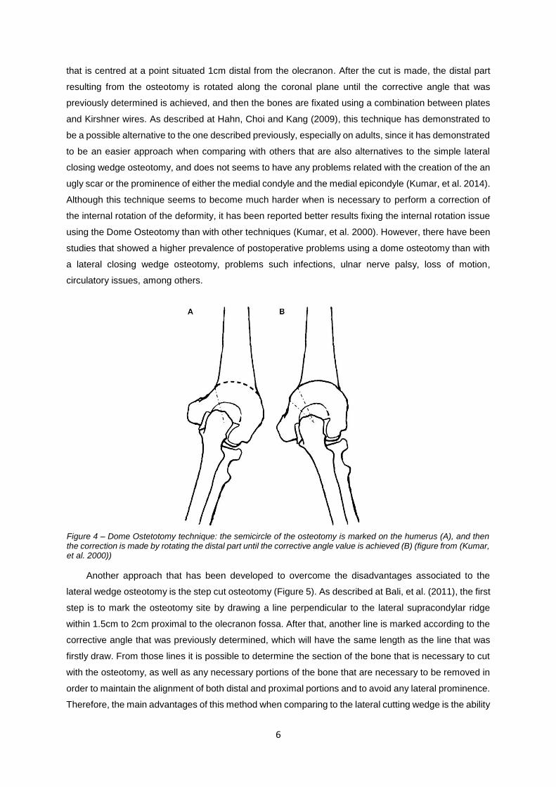


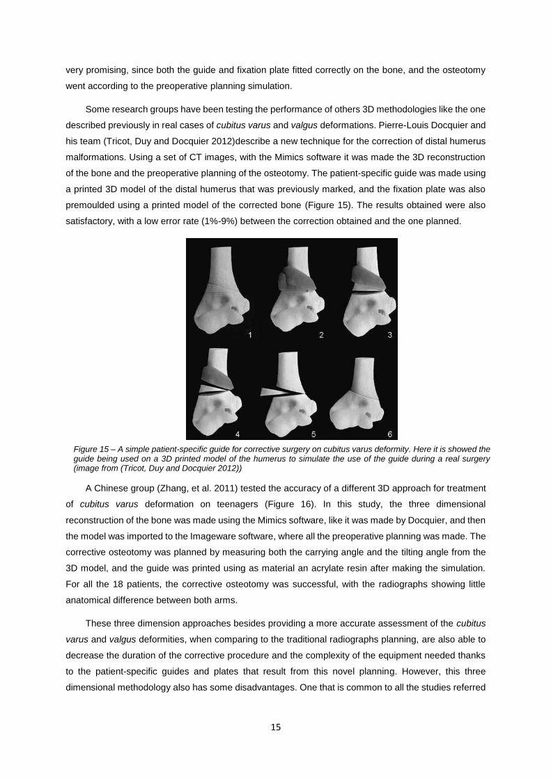


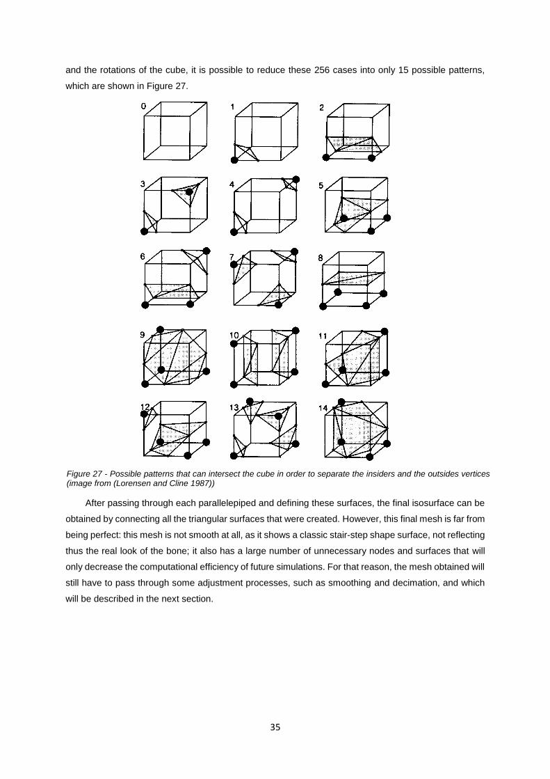


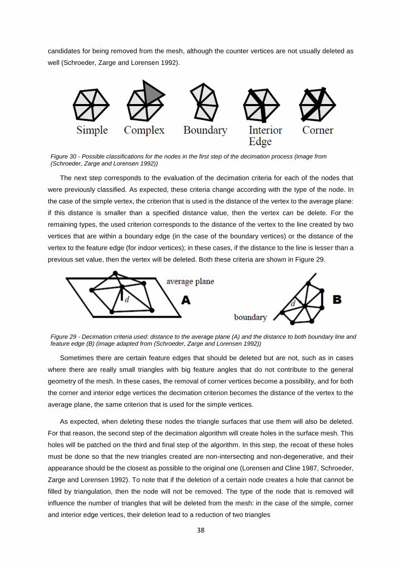

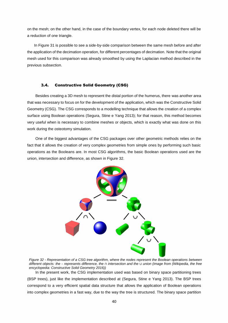


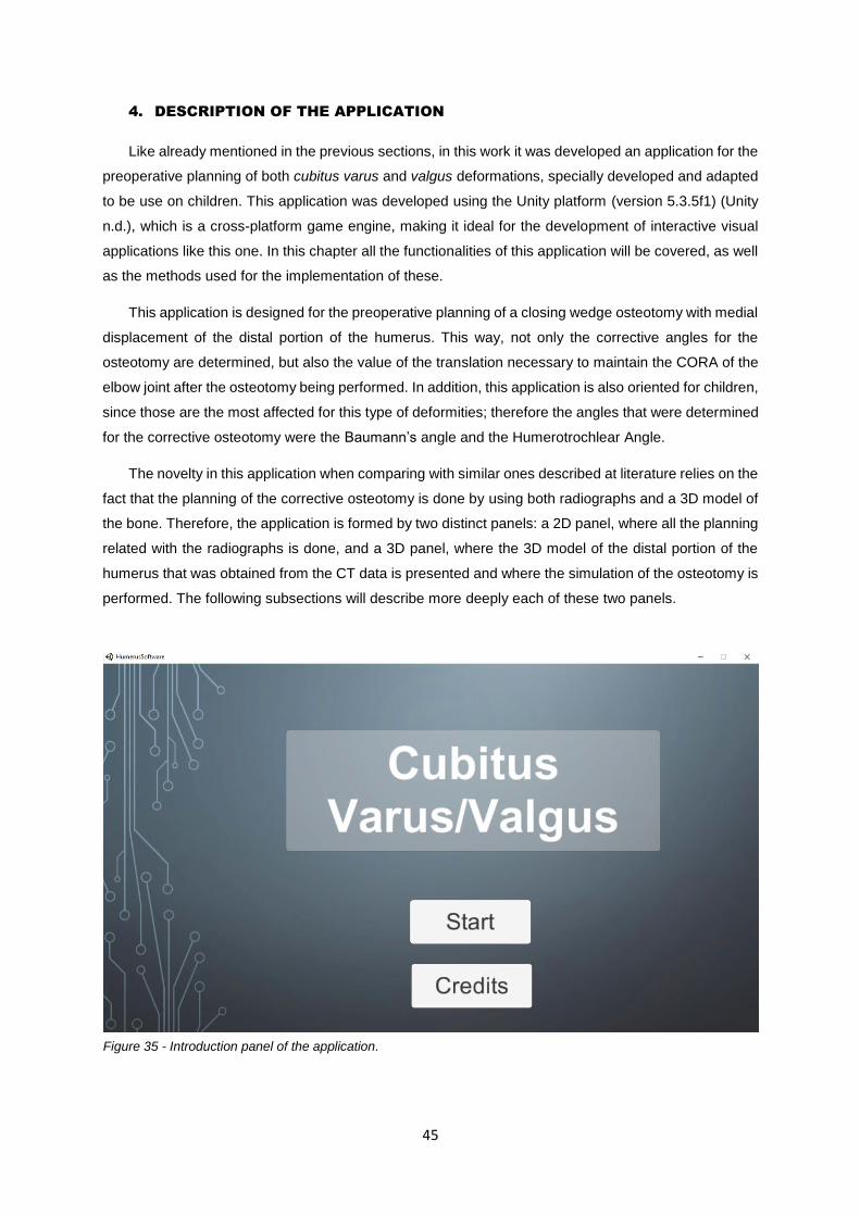

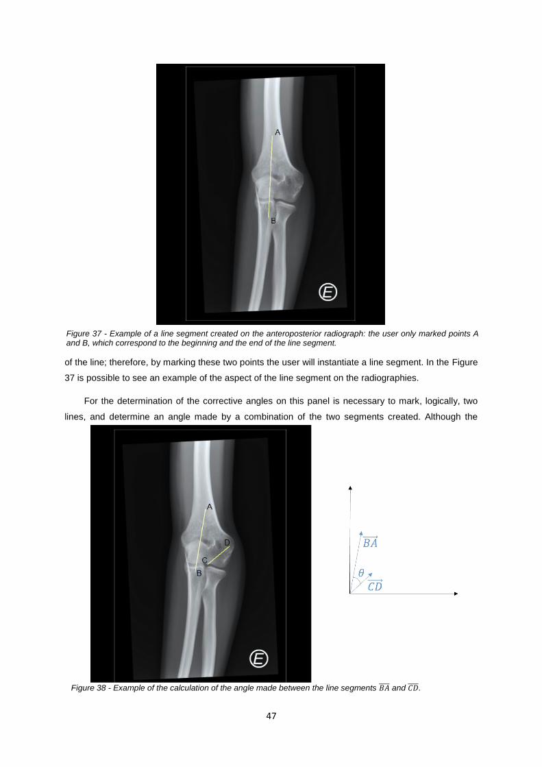


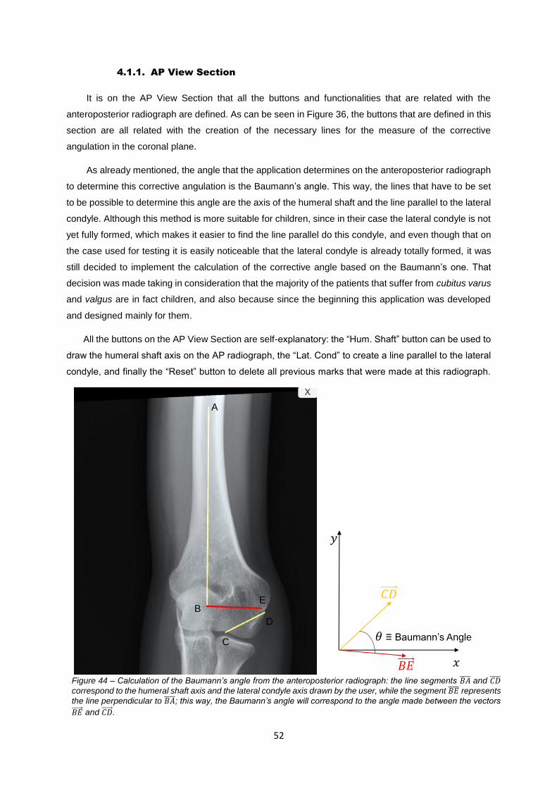

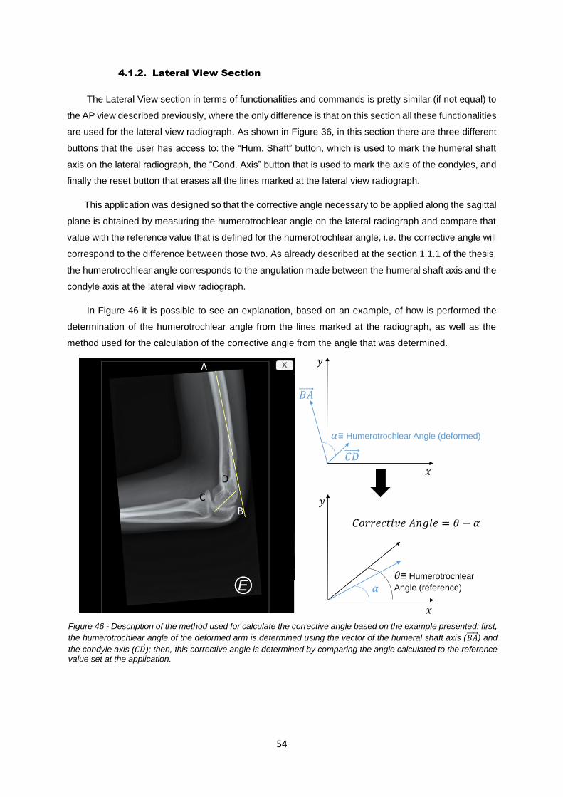
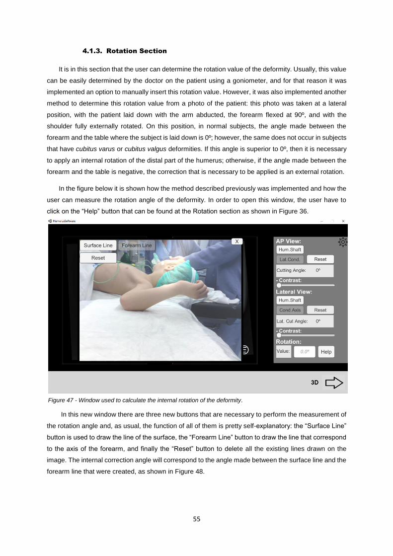


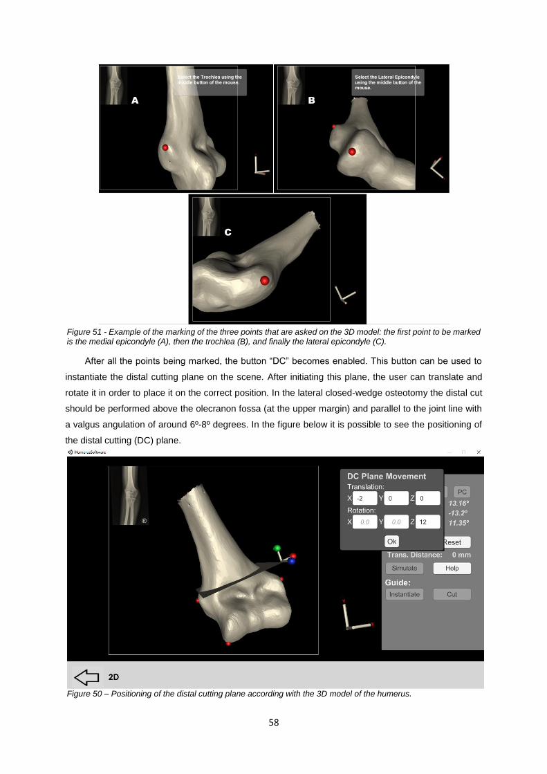

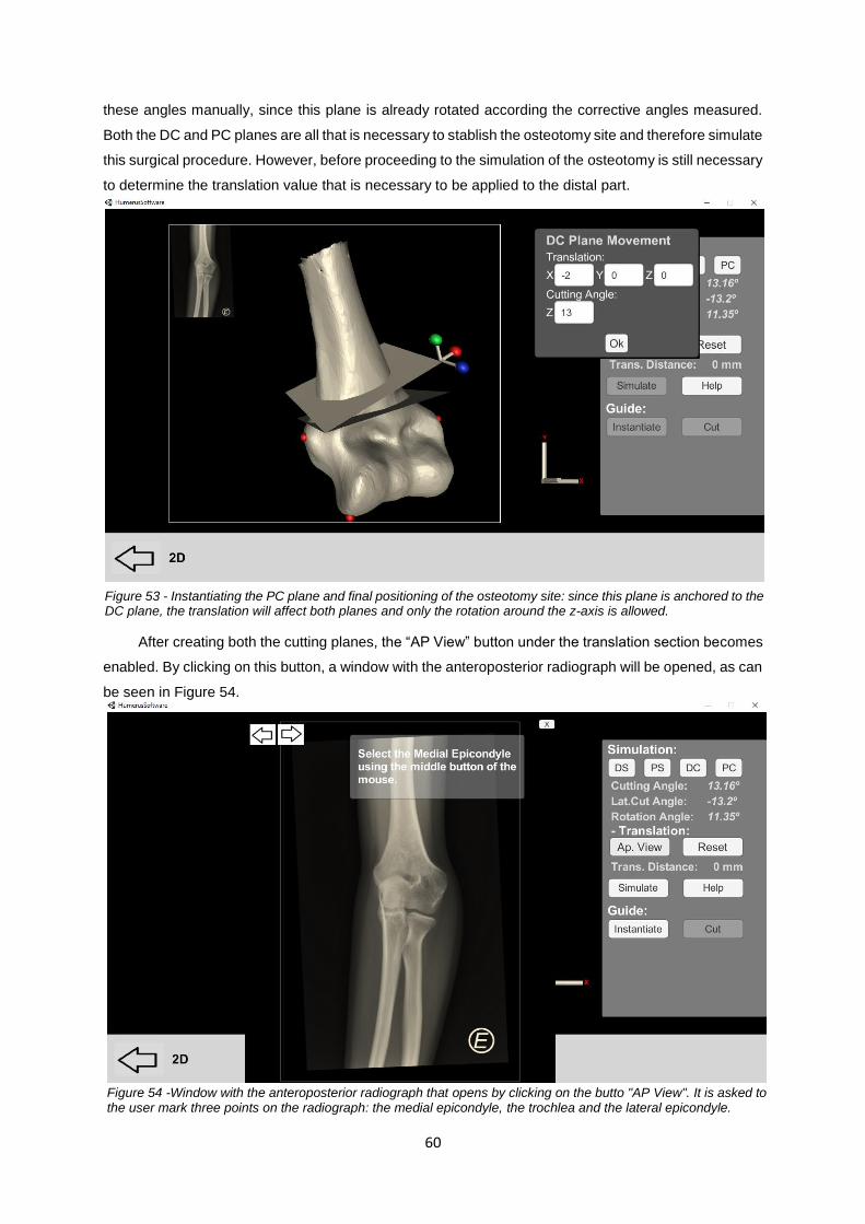
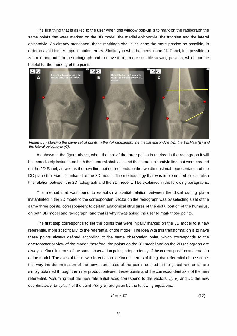


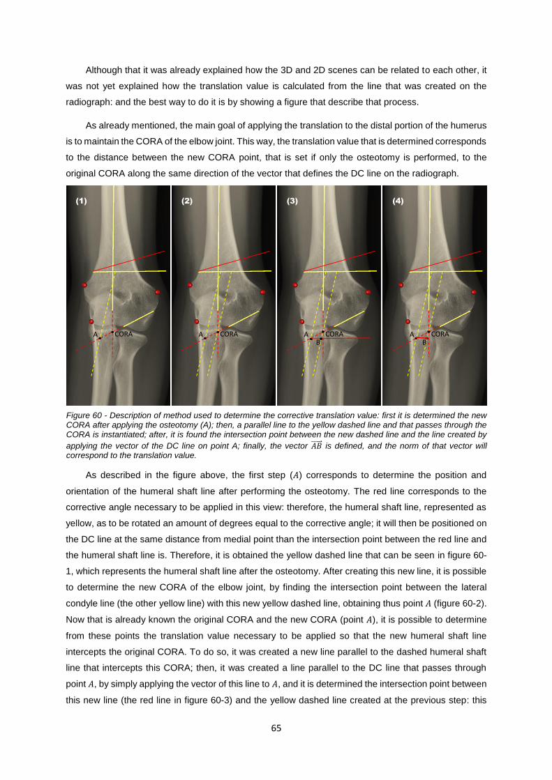
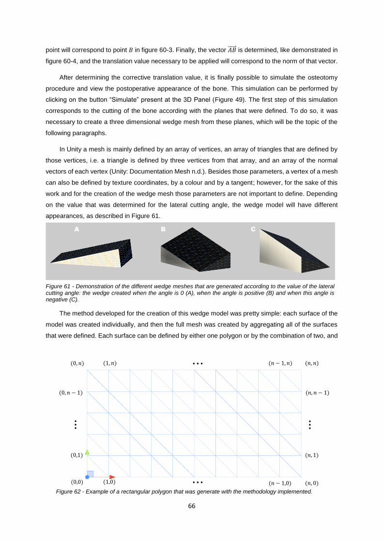


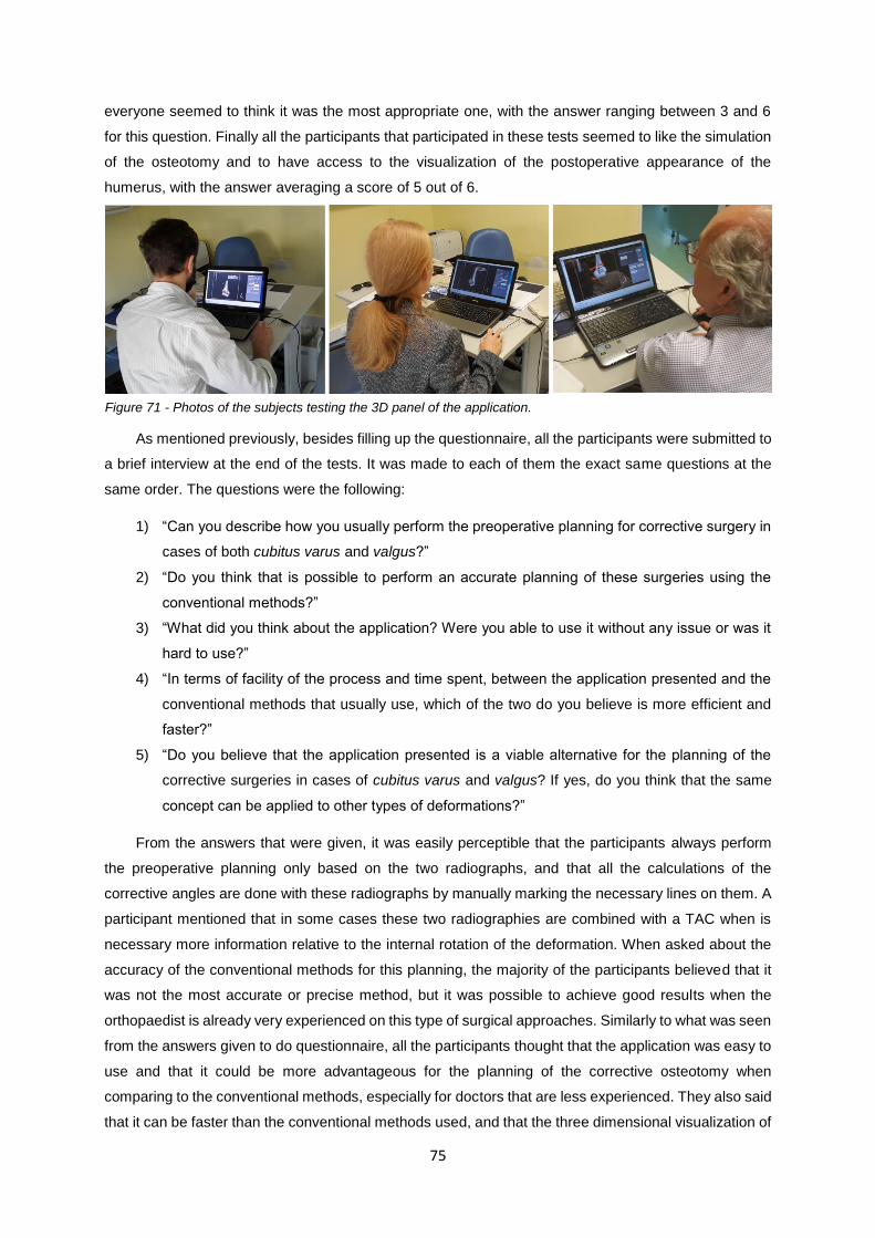


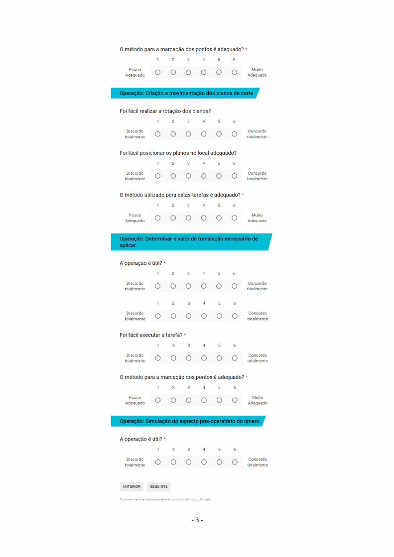


![Pediatric Supracondylar Fractures: Are Medial Pins Indicated?are the supracondylar fractures of the humerus that can be managed by both operative and non-operative modalities [1].](https://static.documents.pub/doc/80x56/6087220d2ec1ae7c713805b2/pediatric-supracondylar-fractures-are-medial-pins-indicated-are-the-supracondylar.jpg)


