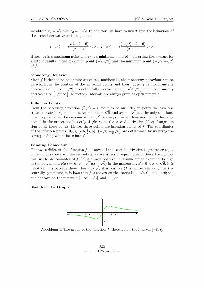
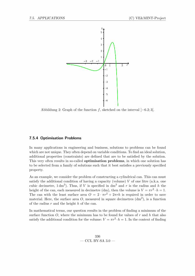
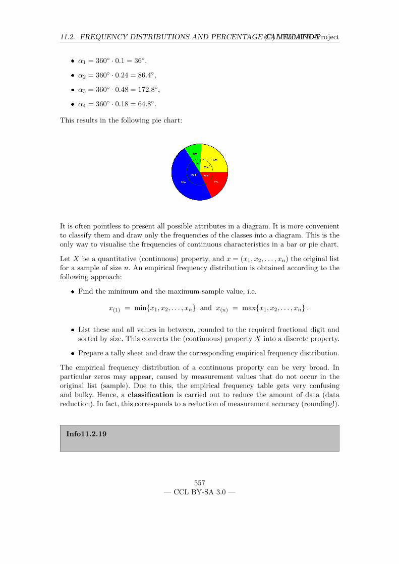
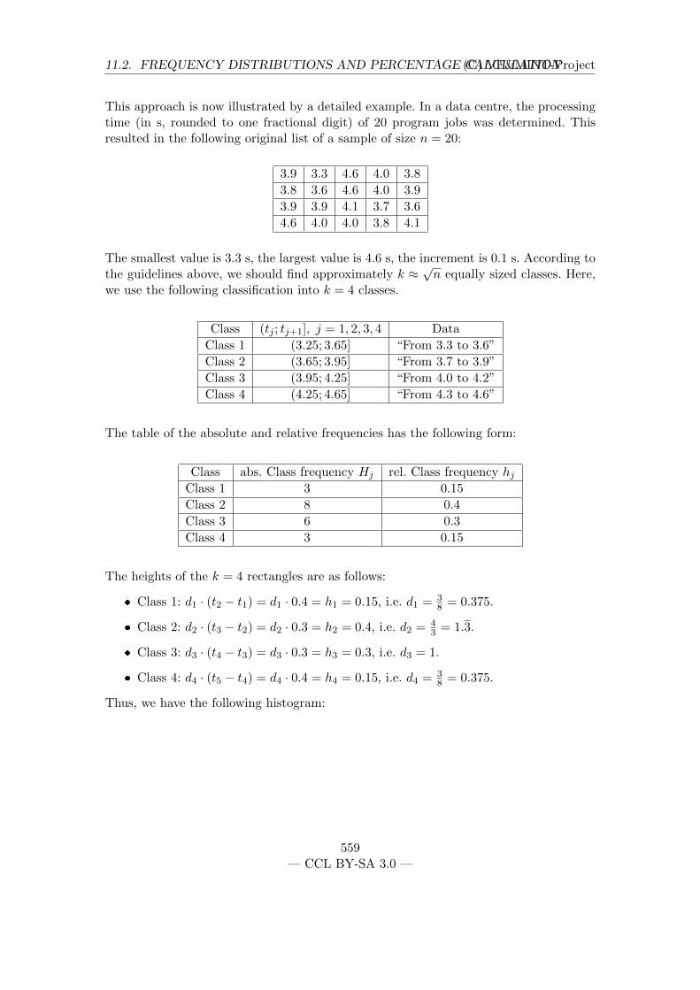
Preparatory Online Course in Mathematics Course version: MFR-TUB(10000) Course date: 09/2016 Local version: DE-MINT Course variant: std [email protected]The courses contents are provided under Creative Commons License CC BY-SA 3.0 and can be copied or used in modified form so long as the origin (the present course) is cited. The course was developed within the scope of the VE&MINT project. VE&MINT is a project cooperation of MINT-Kolleg Baden-W¨ urttemberg with VEMINT- Konsortium, Leibniz Universit¨ at Hannover and Technische Universit¨ at Berlin which seeks to offer a preparatory mathematical online course that is freely accessible nation- wide based on a free licence, and more generally to promote exchange of instructional material as well as software between its sites. For further information on the online course and the project, see www.ve-und-mint.de. The English language/bilingual version of the course was developed at the TU Berlin with the specific goal to create a course accessible and useful for refugees. 1
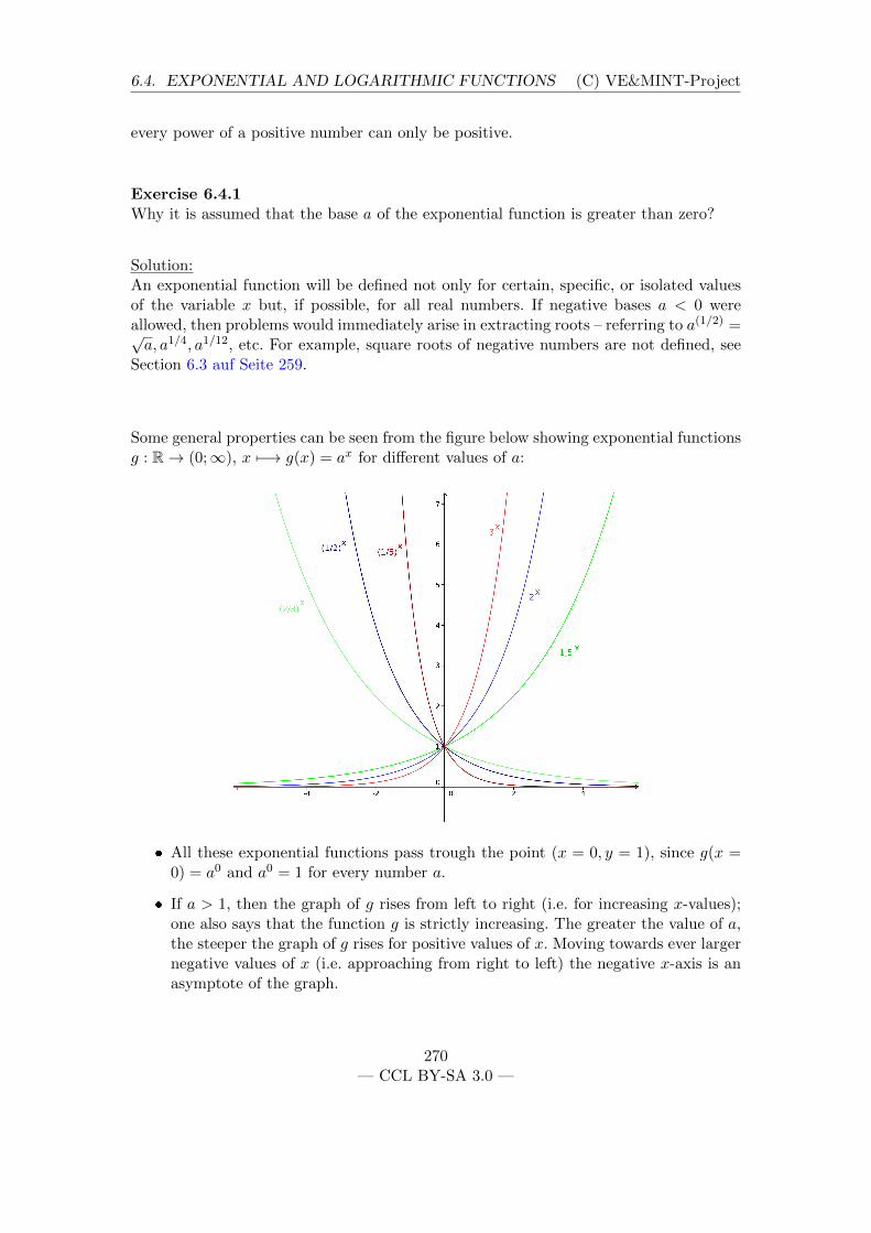
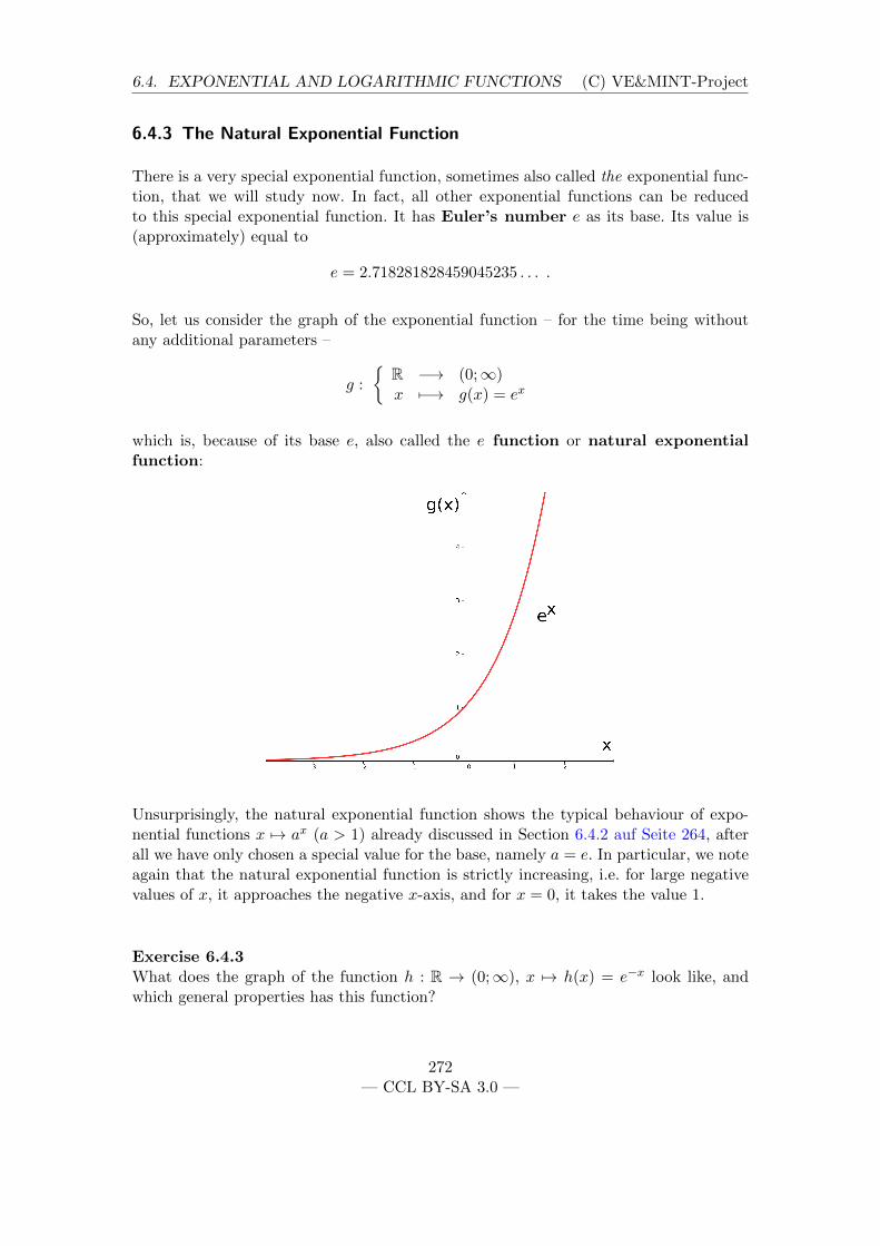
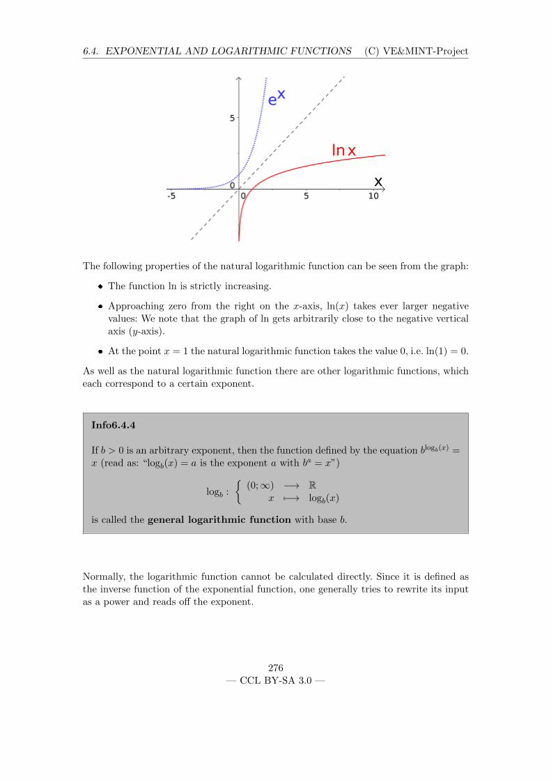
The courses contents are provided under Creative Commons License CC BY-SA 3.0 andcan be copied or used in modified form so long as the origin (the present course) is cited.
The course was developed within the scope of the VE&MINT project.
VE&MINT is a project cooperation of MINT-Kolleg Baden-Wurttemberg with VEMINT-Konsortium, Leibniz Universitat Hannover and Technische Universitat Berlin whichseeks to offer a preparatory mathematical online course that is freely accessible nation-wide based on a free licence, and more generally to promote exchange of instructionalmaterial as well as software between its sites.
For further information on the online course and the project, see www.ve-und-mint.de.
The English language/bilingual version of the course was developed at the TU Berlinwith the specific goal to create a course accessible and useful for refugees.
12.2.1 Graded Test for the Online Course . . . . . . . . . . . . . . . . . . 574
7
1 Elementary Arithmetic
Module Overview
This module covers the mathematical basics of elementary arithmetic and introducesand explains the notation used throughout this online course.
8
1 Elementary Arithmetic (C) VE&MINT-Project
1.1 Numbers, Variables, Terms
1.1.1 Introduction
Mathematics is a science in which abstract structures and the logical relations betweenthem are investigated. Before we examine the actual subjects of this section in moredetail, we shall refer briefly to the fundamental notion of a set.
Info1.1.1
We will often be making statements about a number of structurally similar objects.To do so in a compact manner, we can gather such objects into sets that serve ascontainers for the objects. Let the objects be denoted by a, b, c, . . .. Then the symbolM = a; b; c; . . . denotes the set M which has the previously listed objects as itselements. The latter statement is written in short as a ∈ M , b ∈ M , c ∈ M etc;thus the symbol “∈” reads “is an element of”. (Sometimes it is more convenient toreverse the order of element and set. To do so, we can reverse the symbol ∈, as inM 3 a, M 3 b, M 3 c. The meaning is the same as before, and the reversed symbol“3” reads “contains as an element” or just “contains”.)
Apart from the list notation for sets, other notations exist. If, for example, theelements have to satisfy a condition B, then this is written in the form T = x :x satisfies B. If x is taken (explicitly) from a more comprehensive set U , thenthis is also written in the form T = x : x ∈ U and x satisfies B or, in short,T = x ∈ U : x satisfies B.
Statements like “x ∈ U” or “x satisfies B” are statements in a mathematical sense,i.e. we can assign them a unique truth value “true” or “false”. Let A1 and A2 be twosuch statements. In case both A1 and A2 hold, we write A1 ∧ A2. In case only oneof the two statements needs to hold, i.e. A1 or A2 or both, we write A1 ∨A2.
For two sets M and N we write:
M ⊆ N , i.e. M is a (possibly improper) subset of N , if every element of M isalso an element of N . If at least one element of N exists that is not in M , wesay that M is a proper subset of N . In this case we can also write M ⊂ N .
M ∪N for the union of the two sets. The union denotes the set containing allelements that are contained in at least one of the two sets.
M ∩N for the intersection of the two sets. The intersection denotes the setcontaining all elements that are contained in both of the two sets.
9— CCL BY-SA 3.0 —
1 Elementary Arithmetic (C) VE&MINT-Project
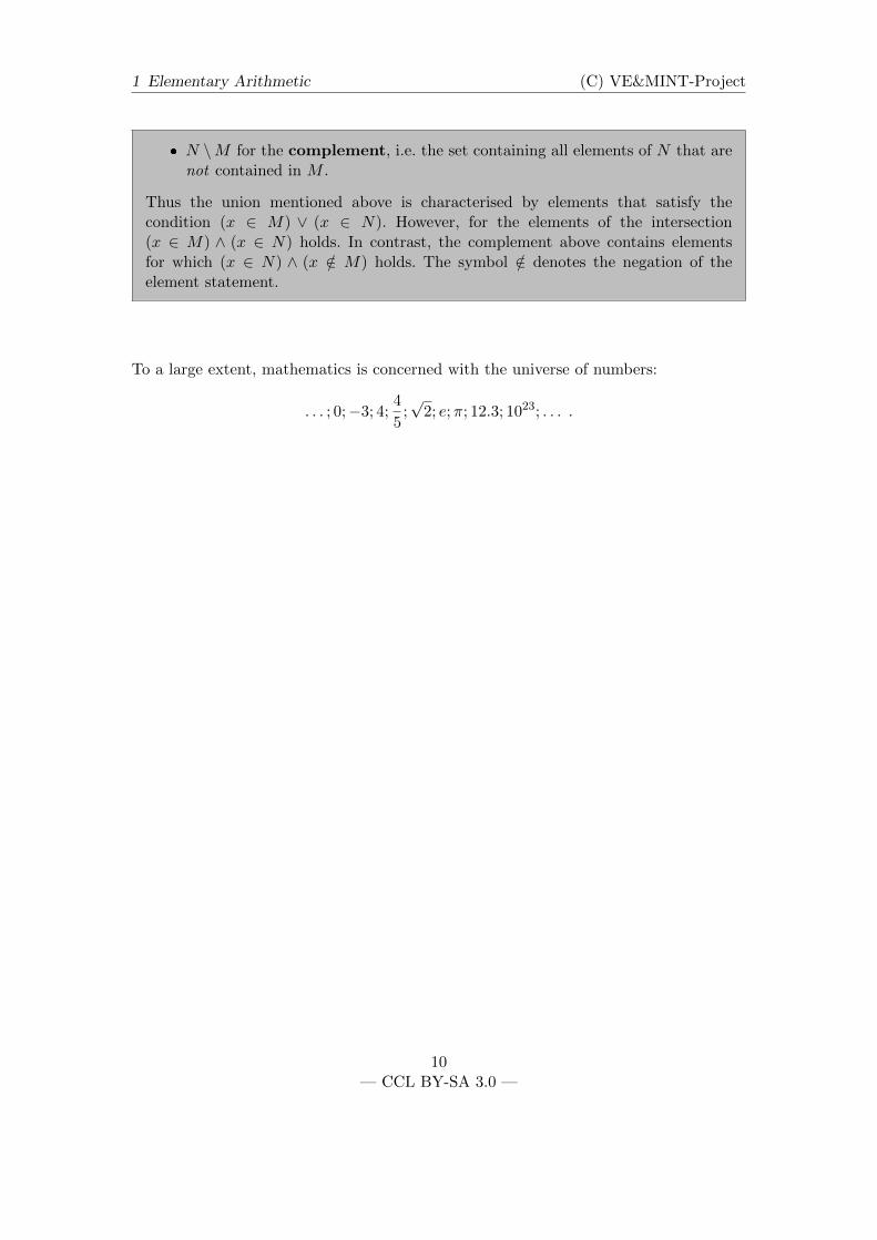
N \M for the complement, i.e. the set containing all elements of N that arenot contained in M .
Thus the union mentioned above is characterised by elements that satisfy thecondition (x ∈ M) ∨ (x ∈ N). However, for the elements of the intersection(x ∈ M) ∧ (x ∈ N) holds. In contrast, the complement above contains elementsfor which (x ∈ N) ∧ (x /∈ M) holds. The symbol /∈ denotes the negation of theelement statement.
To a large extent, mathematics is concerned with the universe of numbers:
. . . ; 0;−3; 4;4
5;√
2; e;π; 12.3; 1023; . . . .
10— CCL BY-SA 3.0 —
1 Elementary Arithmetic (C) VE&MINT-Project
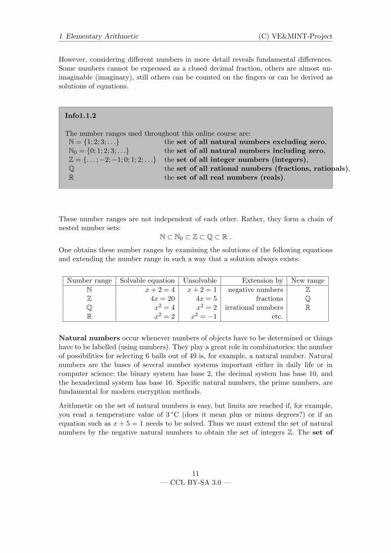
However, considering different numbers in more detail reveals fundamental differences.Some numbers cannot be expressed as a closed decimal fraction, others are almost un-imaginable (imaginary), still others can be counted on the fingers or can be derived assolutions of equations.
Info1.1.2
The number ranges used throughout this online course are:N = 1; 2; 3; . . . the set of all natural numbers excluding zero,N0 = 0; 1; 2; 3; . . . the set of all natural numbers including zero,Z = . . . ;−2;−1; 0; 1; 2; . . . the set of all integer numbers (integers),Q the set of all rational numbers (fractions, rationals),R the set of all real numbers (reals).
These number ranges are not independent of each other. Rather, they form a chain ofnested number sets:
N ⊂ N0 ⊂ Z ⊂ Q ⊂ R .
One obtains these number ranges by examining the solutions of the following equationsand extending the number range in such a way that a solution always exists:
Number range Solvable equation Unsolvable Extension by New range
Natural numbers occur whenever numbers of objects have to be determined or thingshave to be labelled (using numbers). They play a great role in combinatorics: the numberof possibilities for selecting 6 balls out of 49 is, for example, a natural number. Naturalnumbers are the bases of several number systems important either in daily life or incomputer science: the binary system has base 2, the decimal system has base 10, andthe hexadecimal system has base 16. Specific natural numbers, the prime numbers, arefundamental for modern encryption methods.
Arithmetic on the set of natural numbers is easy, but limits are reached if, for example,you read a temperature value of 3 C (does it mean plus or minus degrees?) or if anequation such as x+ 5 = 1 needs to be solved. Thus we must extend the set of naturalnumbers by the negative natural numbers to obtain the set of integers Z. The set of
11— CCL BY-SA 3.0 —
1 Elementary Arithmetic (C) VE&MINT-Project
integers is denoted by
Z := . . . ;−4;−3;−2;−1; 0; 1; 2; 3; 4; . . . .
Integers are required whenever the sign (plus or minus) of a natural number matters. InZ, numbers can be subtracted from each other without any restriction, i.e. systems ofequations of the form a+ x = b are always solvable in Z (x = b+ (−a)).
−5 −4 −3 −2 −1 0 1 2 3 4 5 6
On the set of integers a comparator < can be uniquely defined, so that the integers canbe ordered into a chain:
· · · < −3 < −2 < −1 < 0 < 1 < 2 < 3 < . . . .
12— CCL BY-SA 3.0 —
1 Elementary Arithmetic (C) VE&MINT-Project
A rational number (rational) is the ratio of two integers:
Info1.1.3
The set of rational numbers is denoted by
Q :=
p
q: p, q ∈ Z, q 6= 0
.
The elements pq of the set Q are called fractions, where p is the numerator of the
fraction and q is the non-zero denominator of the fraction.
The rationals play a role whenever the numbers have to be “more precise”, e.g. if tem-peratures have to be given in fractional amounts of C, parts of surfaces have to becoloured, or medications have to be mixed from specific ingredients.
Note that the representation as a fraction is not unique: one number can be representedby several fractions. For example,
2 =4
2=
1024
512
all represent the same rational number.
Also, not every number on the number line can be represented as a fraction. Considering,for example, a square with sides of length 1, the length of the diagonal d can be calculatedby means of the Pythagoras’ theorem:
d
1 cm
d2 = 12 + 12 = 2, or formally, d =√
2.
Another number that cannot be represented as a fraction is obtained by unrolling awheel of diameter 1 on the number line. The result is the number π. It can be proventhat these two numbers (
√2 and π) cannot be represented as fractions. (In the case
13— CCL BY-SA 3.0 —
1 Elementary Arithmetic (C) VE&MINT-Project
of√
2 this proof is relatively simple.) These numbers are two examples of the so-calledirrational numbers.
x0 Pi
A number is irrational if it is not rational, i.e. if it cannot be represented as a fraction.The irrational numbers close the remaining gaps on the number line, where every pointnow corresponds to exactly one real number.
Info1.1.4
The set of real numbers is denoted by R and includes the set of rational numbersand the set of irrational numbers. It contains all numbers that can be representedon the number line.
Real numbers serve as measures for lengths, areas, temperatures, masses, etc. Throug-hout this course the mathematical problems are typically solved using real numbers.
A basic property of the real numbers is that they are ordered, i.e. for two reals a, bexactly one of the three relations a < b, a = b, or a > b holds. Another defining propertyis completeness, which – roughly speaking – describes the “gaplessness” of the numberline.
Info1.1.5
For two different real numbers, one sometimes considers all reals lying between thesetwo numbers on the number line. Such a set of reals is called an interval. An intervalis described by assigning a left interval boundary (a) and a right interval boundary(b) with a < b. Depending on whether each interval boundary is included, we mustdistinguish the following cases:
x ∈ R : x ≥ a and x ≤ b = [a; b] denotes the closed interval between a and
14— CCL BY-SA 3.0 —
1 Elementary Arithmetic (C) VE&MINT-Project
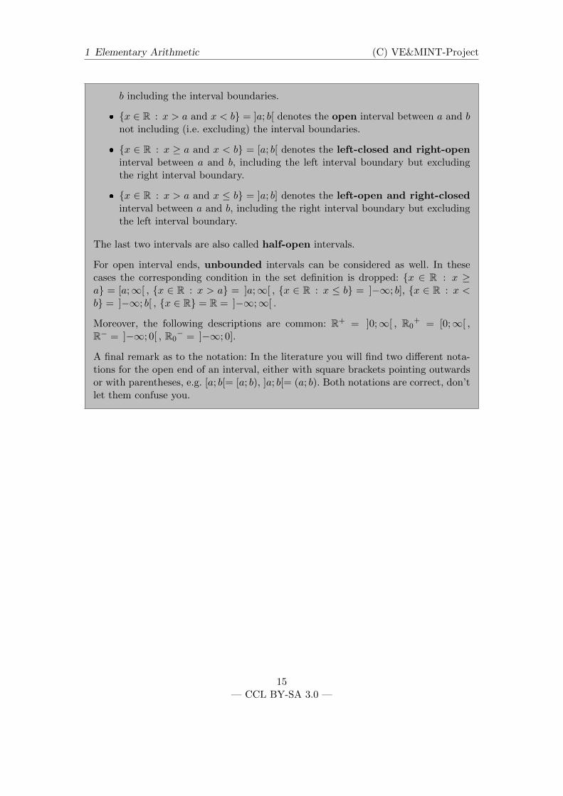
b including the interval boundaries.
x ∈ R : x > a and x < b = ]a; b[ denotes the open interval between a and bnot including (i.e. excluding) the interval boundaries.
x ∈ R : x ≥ a and x < b = [a; b[ denotes the left-closed and right-openinterval between a and b, including the left interval boundary but excludingthe right interval boundary.
x ∈ R : x > a and x ≤ b = ]a; b] denotes the left-open and right-closedinterval between a and b, including the right interval boundary but excludingthe left interval boundary.
The last two intervals are also called half-open intervals.
For open interval ends, unbounded intervals can be considered as well. In thesecases the corresponding condition in the set definition is dropped: x ∈ R : x ≥a = [a;∞[ , x ∈ R : x > a = ]a;∞[ , x ∈ R : x ≤ b = ]−∞; b], x ∈ R : x <b = ]−∞; b[ , x ∈ R = R = ]−∞;∞[ .
Moreover, the following descriptions are common: R+ = ]0;∞[ , R0+ = [0;∞[ ,
R− = ]−∞; 0[ , R0− = ]−∞; 0].
A final remark as to the notation: In the literature you will find two different nota-tions for the open end of an interval, either with square brackets pointing outwardsor with parentheses, e.g. [a; b[= [a; b), ]a; b[= (a; b). Both notations are correct, don’tlet them confuse you.
15— CCL BY-SA 3.0 —
1 Elementary Arithmetic (C) VE&MINT-Project
1.1.2 Variables and Terms
The use of variables, terms and equations is required to formalise expressions whosevalues have not been fixed.
Info1.1.6
A variable is a symbol (typically a letter) used as a placeholder for an indeterminatevalue. A term is a mathematical expression that can contain variables, arithmeticoperations and further symbols and, after substituting variables with numbers, canbe evaluated to a specific value. Terms can be combined into equations and inequa-lities, respectively, or they can be inserted into function descriptions, as we shall seelater.
Example 1.1.7
The word problem
In a school class there are four more girls than boys and in total there are 20 children.How many girls and boys are in the class, respectively?
can be formalised, for example, by introducing the variable a for the number ofgirls and the variable b for the number of boys in the class and setting up the twoequations a = b+ 4 and a+ b = 20. These equations can be solved by inserting thefirst equation into the second which gives a = 12 and b = 8. Out of this, the fullwritten answer
In the school class there are 12 girls and 8 boys
can be constructed. Here, for example, b + 4 is a term, b itself is a variable, anda+ b = 20 is an equation with a term on the left and a number on the right.
Variables (and sometimes also terms) are generally denoted by Latin lowercase lettersx, y, z, etc. Often Greek letters are used as well, for example, to distinguish variablesthat represent angles from those that represent numbers.
16— CCL BY-SA 3.0 —
1 Elementary Arithmetic (C) VE&MINT-Project
Info1.1.8
This overview shows the (lowercase and uppercase) letters of the Greek alphabet inGreek alphabetical order:
α, A “alpha” β, B “beta” γ, Γ “gamma” δ, ∆ “delta” ε, E “epsilon”ζ, Z “zeta” η, H “eta” ϑ, Θ “theta” ι, I “iota” κ, K “kappa”λ, Λ “lambda” µ, M “mu” ν, N “nu” ξ, Ξ “xi” o, O “omicron”π, Π “pi” %, P “rho” σ, Σ “sigma” τ , T “tau” υ, Υ “upsilon”ϕ, Φ “phi” χ, X “chi” ψ, Ψ “psi” ω, Ω “omega”
It is important that a term can be evaluated to a specific value if the variables occurringin the term are substituted with numbers:
17— CCL BY-SA 3.0 —
1 Elementary Arithmetic (C) VE&MINT-Project
Example 1.1.9
The following expressions are terms:
x · (y + z)− 1: for x = 1, y = 2, and z = 0 one obtains, for example, the value1.
sin(α) + cos(α): for α = 0 and β = 0 one obtains, for example, the value 1(for the calculation of sine and cosine refer to 5).
1 + 2 + 3 + 4: no variables occur, however this is a term (which always givesthe value 10).
α+β1+γ : for example, α = 1, β = 2, and γ = 3 give the value 3
4 . But γ = −1 isnot allowed.
sin(π(x+ 1)): this term, for example, always gives the value zero if x is substi-tuted with an integer.
z: a single variable is also a term.
1 + 2 + 3 + · · · + (n − 1) + n is a term, in which the variable n occurs in theterm itself and defines its length as well.
Example 1.1.10
These expressions are not terms in a mathematical sense:
a + b = 20 is an equation (inserting values for a and b gives no number, butthe equation is simply true or false).
a · (b+ c is not correctly bracketed,
“The ratio of girls in the school class” is not a term, but can be formalised bythe term a
a+b ,
sin is not a term but a function name, in contrast sin(α) is a term (which canbe evaluated by inserting an angle for α).
Exercise 1.1.1In each question, given a term and number values for the variables that occur in it, whatis the evaluation of the term?
18— CCL BY-SA 3.0 —
1 Elementary Arithmetic (C) VE&MINT-Project
a. α+βα−β takes the value for α = 6 and β = 4.
b. y2 + x2 takes the value for y = 2x+ 1 and x = −1.
c. 1 + 2 + 3 + · · ·+ (n− 1) + n takes the value for n = 6.
Solution:After inserting the given values for the variables, the term evaluates to a) α+β
α−β = 6+46−4 =
102 = 5, b) y2 + x2 = (−1)2 + (−1)2 = 2, and c) 1 + 2 + 3 + 4 + 5 + 6 = 21.
Exercise 1.1.2Formalise, using the variables given, the proportion of girls and the proportion of boys,the number of girls being denoted by the variable a and the number of boys by thevariable b:
The proportion of girls is and the proportion of boys is.
Solution:The total number of children is a + b, hence the proportion of girls is a
a+b and the
proportion of boys is ba+b .
Terms can be inserted into other terms as well:
Info1.1.11
When inserting terms, a term is substituted for a symbol in another term. If theterm to be inserted contains several expressions, the replaced symbol has to bebracketed in advance.
Example 1.1.12
Substituting, for example, the right-hand side of x = 1 + 2 + 3 into the term x2 + y2
results in the new term x2 + y2 = (1 + 2 + 3)2 + y2 = 36 + y2 and certainly not1 + 2 + 32 + y2 = 12 + y2.
19— CCL BY-SA 3.0 —
1 Elementary Arithmetic (C) VE&MINT-Project
Exercise 1.1.3Which term is formed if the following object is inserted into the term x2 + y2?
a. The angle α both for x and y: Then x2 + y2 = .
b. The number 2 for y and the term t+ 1 for x: Then x2 + y2 = .
c. The term z + 1 for x and the term z− 1 for y: Then x2 + y2 = .
Solution:It is safest to bracket the variables before inserting, if the new term contains severalsymbols:
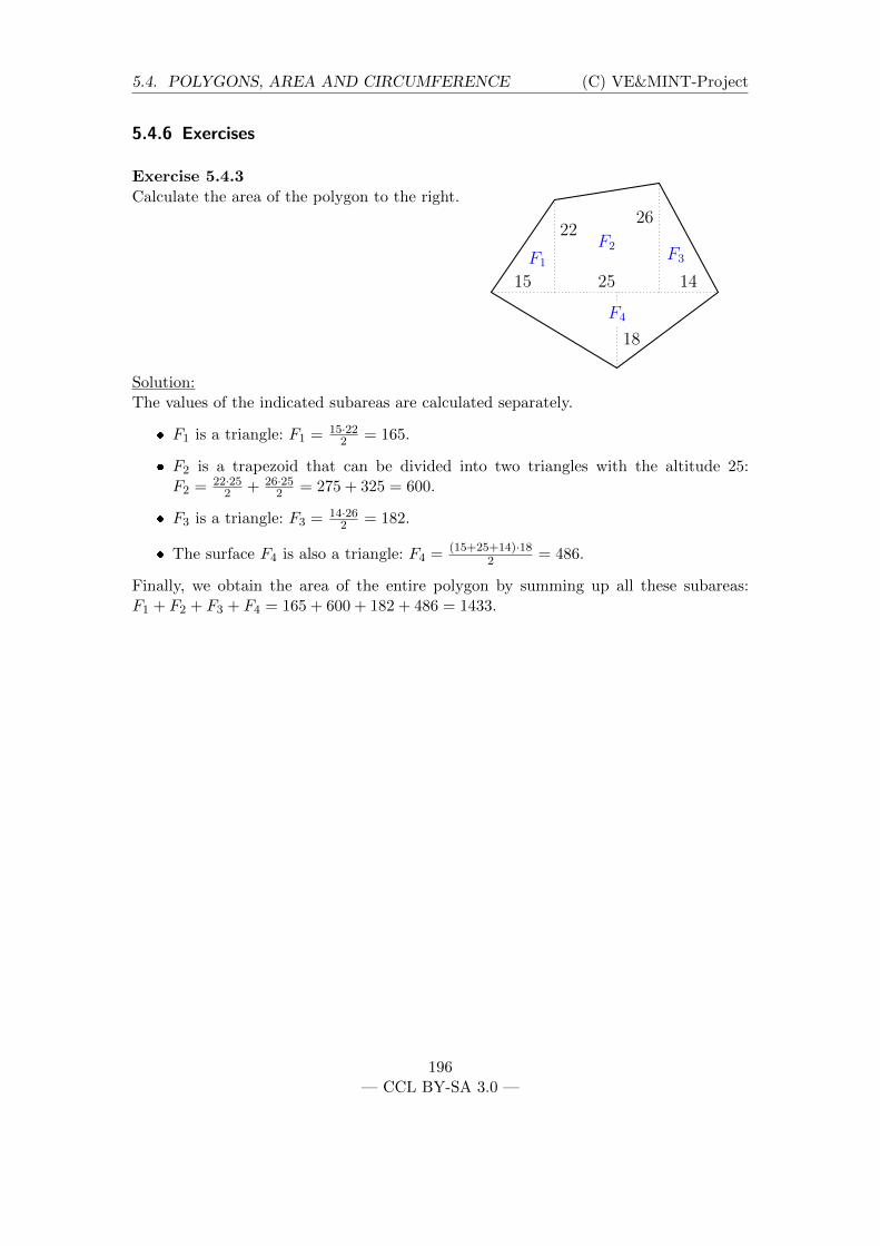
Exercise 1.1.4In the following figure, a square on the paper has side length x. What is the area of thisfigure (as a term in the variable x)?
(A single square has side length x)
A figure on squared paper.
Answer:
The large circle has a total area of ,
each smaller circle has an area of ,
20— CCL BY-SA 3.0 —
1 Elementary Arithmetic (C) VE&MINT-Project
the total area of the figure is .
Hint for calculating the area:The calculation of areas is presented in later chapters. To solve this exercise, you onlyneed to know that a rectangle of side lengths a and b has the area a · b (entered as a*b)and a circle of radius r has the area πr2 (entered as pi*r2).
Solution:The large circle has in total the area 25
4 πx2 (entered as 25/4*pi*x*x). Each smaller
circle has the area 14πx
2, and the whole figure has the area (254 π −
12π − 3) · x2.
1.1.3 Transformation of terms
There is always more than one way to write the same term, although some are morenatural than others. For example, x+ x is a different arrangement of symbols than 2x,but describes the same term, i.e. if x is substituted with a specific number, then x + xand 2x provide the same value.
Info1.1.13
Terms are related by an equals sign if they are always evaluated to the same value.
In general, new terms are created by transformation of existing terms:
Info1.1.14
A transformation of a term is created by applying one or more calculation rulesto the term:
Collecting: a+ a+ · · ·+ a = n · a (n is the number of summands).
Distributive property (“expansion”): (a+b) ·c = ac+bc and c ·(a+b) = ca+cb.
Commutative property: a+ b = b+ a.
Associative property (“group numbers differently in operations of the same
21— CCL BY-SA 3.0 —
1 Elementary Arithmetic (C) VE&MINT-Project
kind”):a+ (b+ c) = (a+ b) + c = a+ b+ c, also possible in multiplications.
Calculation rules for powers and special functions.
Calculation rules for specific types of terms (e.g. the binomial formulas).
Calculation rules for fractions: 1ab
= ba .
The rules will be presented in detail in the following sections. Often, the aim of thistransformation is to simplify the term, to isolate individual variables, or to transform aterm into a certain form:
Example 1.1.15
Examples of transformations and their uses:
a(a + a + a) + a2 + a2 + a2 = 6a2: the term on the right is simpler, since itrequires fewer symbols.
(x+3)2−9 = x2 +6x (first binomial formula): both terms describe a parabola.On the left, the vertex (−3,−9) of the parabola can be seen easily, on the right,the two roots (x1 = 0 and x2 = −6) can be seen easily.
1 + 3x + 3x2 + x3 = (1 + x)3: on the right, it can be seen, for example, thatthe function described by the term has only the root x1 = −1.
a+1a = 1 + 1
a : on the left, it can be seen that the term has the root a1 = −1, onthe right it can be seen that, for very large a, the term converges to 1 (since 1
ais very small in this case).
Exercise 1.1.5Transform into a sum: a · (b+ c) + c · (a+ b) = .Solution:
a · (b+ c) + c · (a+ b) = ab+ ac+ ca+ cb = ab+ 2ac+ bc
22— CCL BY-SA 3.0 —
1 Elementary Arithmetic (C) VE&MINT-Project
Exercise 1.1.6Transform into a sum: (x− y)(z − x) + (x− z)(y − z) = .Solution:
A fraction is a rational number written in the form numeratordenominator
, where numerator anddenominator are integers, and the denominator is 6= 0. Examples are:
1
2,
5
−10,−17
12,
1
23,
4
6,−2
3, . . . .
It can be seen very quickly that a single number can have an arbitrary number ofequivalent representations. For example:
12
36=
1
3=
24
72=−12
−36=
3
9=
2
6=
120
360= . . . .
The different representations transform into each other by reducing and expanding,respectively.
Info1.2.1
Fractions are reduced by dividing numerator and denominator by the same non-zerointeger.
Fractions are expanded by multiplying numerator and denominator by the samenon-zero integer.
Example 1.2.2
Three friends like to share a pizza. Tom eats 14 of the pizza, Tim eats 1
3 of the pizza.How much of the pizza is left for their friend Sven, who always has the biggestappetite?The solution is found by means of fractional arithmetic: First, we have to add twofractions, to decide how much of the pizza Tim and Tom already ate:
1
4+
1
3=
1 · 34 · 3
+1 · 43 · 4
=3
12+
4
12=
7
12.
Here, we can already identify the two most important steps: First we have to expandthe two fractions to the so-called least common denominator, or, as one also says,we have to create like fractions. Then, if the fractions have the same denominator,we can add them by adding their numerators and maintaining the same denominator.
24— CCL BY-SA 3.0 —
1.2. FRACTIONAL ARITHMETIC (C) VE&MINT-Project
From the result that Tim and Tom ate 712 of the pizza, we can calculate how much
of the pizza is left for Sven by subtracting 712 from 1:
1− 7
12=
12
12− 7
12=
5
12.
Again, we must expand the fractions to the least common denominator. Then wehave to subtract the two numerators. Indeed, the two friends have left much of thepizza for the always hungry Sven.soweit
The reducing of fractions can be practised in the training exercises below.
In the online version, exercises from an exercise list will be shown here
25— CCL BY-SA 3.0 —
1.2. FRACTIONAL ARITHMETIC (C) VE&MINT-Project
It becomes more difficult if indeterminate expressions (e.g. variables) occur in numeratorand denominator. These can be reduced or cancelled just like numbers (but not withnumbers), for example, we get
4x2y3 + 3y2
10y2=
4x2y + 3
10
by cancelling the term y2 from numerator and denominator. The following trainingexercise has been extended to fractions including indeterminate expressions.
In the online version, exercises from an exercise list will be shown here
Info1.2.3
The least common denominator of two fractions is the least common multiple(lcm) of the two denominators.
The least common multiple (lcm) of two numbers is the smallest number that isdivisible by both numbers.
The greatest common divisor (gcd) of two numbers is the largest number thatdivides both numbers without remainder.
If the determination of the lcm is too complicated, the simple product of the denomina-tors can be used instead of the lcm in the following calculation rule:
Info1.2.4
Fractions are added/subtracted by finding a common denominator and thenadding/substracting the numerators, i.e.
a
b± c
d=ad± bcbd
, bd 6= 0 .
Usually fractions are expanded to the least common denominator.
For example, the least common multiple of 6 = 2 · 3 and 15 = 3 · 5 is the number2 · 3 · 5 = 30. However, the product is 6 · 15 = 90. Thus, you can calculate
1
6+
1
15=
5
30+
2
30=
7
30
26— CCL BY-SA 3.0 —
1.2. FRACTIONAL ARITHMETIC (C) VE&MINT-Project
but also1
6+
1
15=
15
90+
6
90=
21
90
and finally reduce the last fraction to 730 .
Example 1.2.5
The least common multiple for the least common denominator is the smallest num-ber that can be divided by all denominators involved. If these denominators have nofactors in common, the least common multiple is simply the product of all denomi-nators:
1
6+
1
10=
5
30+
3
30=
8
30=
4
15,
1
6+
1
10=
10
60+
6
60=
16
60=
4
15(also correct),
4
15− 1
2=
8
30− 15
30=
8− 15
30= − 7
30,
1
3+
1
9=
3
9+
1
9=
4
9,
1
22+
1
24=
22
24+
1
24=
5
16,
1
2+
1
3+
1
7=
21
42+
14
42+
6
42=
41
42.
The least common denominator can also be found if the denominators include variables.Since the transformations of the fractions have to be correct for all possible values ofthese variables, they have to be considered as numbers without any common factors:
Example 1.2.6
Let x and y be variables, then
1
3+
1
x=
x
3 · x+
3
3 · x=
3 + x
3 · x,
1
x+
1
y=
y
x · y+
x
x · y=
x+ y
x · y,
1
(x+ 1)2+
1
x+ 1=
1
(x+ 1)2+
x+ 1
(x+ 1)2=
x+ 2
(x+ 1)2.
27— CCL BY-SA 3.0 —
1.2. FRACTIONAL ARITHMETIC (C) VE&MINT-Project
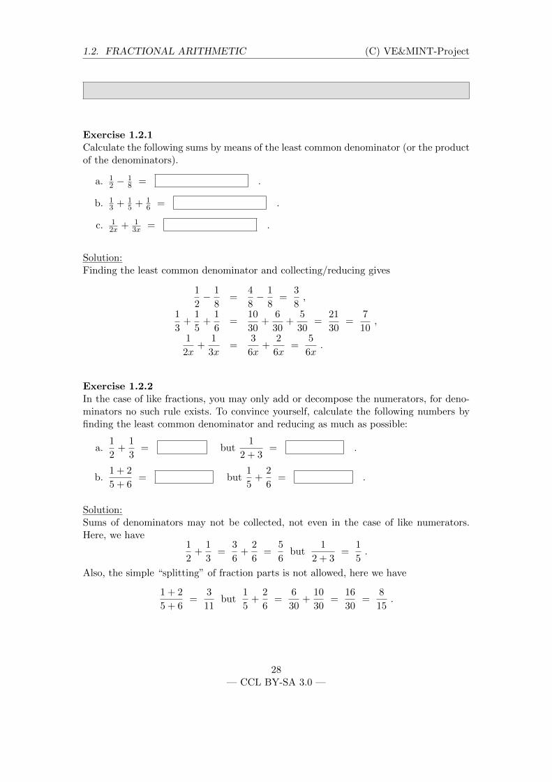
Exercise 1.2.1Calculate the following sums by means of the least common denominator (or the productof the denominators).
a. 12 −
18 = .
b. 13 + 1
5 + 16 = .
c. 12x + 1
3x = .
Solution:Finding the least common denominator and collecting/reducing gives
1
2− 1
8=
4
8− 1
8=
3
8,
1
3+
1
5+
1
6=
10
30+
6
30+
5
30=
21
30=
7
10,
1
2x+
1
3x=
3
6x+
2
6x=
5
6x.
Exercise 1.2.2In the case of like fractions, you may only add or decompose the numerators, for deno-minators no such rule exists. To convince yourself, calculate the following numbers byfinding the least common denominator and reducing as much as possible:
a.1
2+
1
3= but
1
2 + 3= .
b.1 + 2
5 + 6= but
1
5+
2
6= .
Solution:Sums of denominators may not be collected, not even in the case of like numerators.Here, we have
1
2+
1
3=
3
6+
2
6=
5
6but
1
2 + 3=
1
5.
Also, the simple “splitting” of fraction parts is not allowed, here we have
1 + 2
5 + 6=
3
11but
1
5+
2
6=
6
30+
10
30=
16
30=
8
15.
28— CCL BY-SA 3.0 —
1.2. FRACTIONAL ARITHMETIC (C) VE&MINT-Project
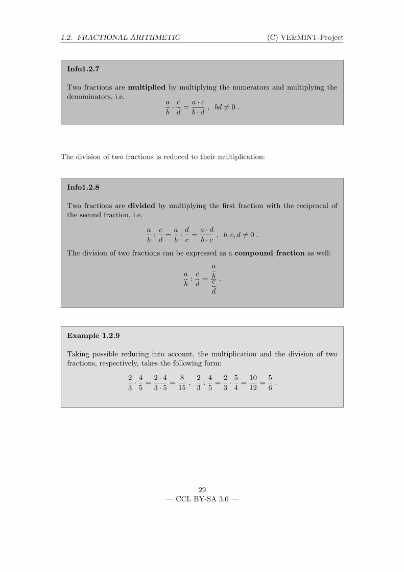
Info1.2.7
Two fractions are multiplied by multiplying the numerators and multiplying thedenominators, i.e.
a
b· cd
=a · cb · d
, bd 6= 0 .
The division of two fractions is reduced to their multiplication:
Info1.2.8
Two fractions are divided by multiplying the first fraction with the reciprocal ofthe second fraction, i.e.
a
b:c
d=a
b· dc
=a · db · c
, b, c, d 6= 0 .
The division of two fractions can be expressed as a compound fraction as well:
a
b:c
d=
a
bc
d
.
Example 1.2.9
Taking possible reducing into account, the multiplication and the division of twofractions, respectively, takes the following form:
2
3· 4
5=
2 · 43 · 5
=8
15,
2
3:
4
5=
2
3· 5
4=
10
12=
5
6.
29— CCL BY-SA 3.0 —
1.2. FRACTIONAL ARITHMETIC (C) VE&MINT-Project
1.2.2 Converting Fractions
Dividing the denominator into the numerator gives a decimal fraction or a decimalnumber, respectively, for example,
1
2= 0.5 ,
1
3= 0.33333 . . . = 0.3 ,
1
7= 0.142857 ,
1
8= 0.125 .
By means of these examples, it can already be seen that the division is either finite,leading to a proper decimal fraction, or the digits of the decimal number repeat in acertain way, leading to an infinite repeating decimal fraction.
Converting decimal numbers to fractions is done using the base-10 positional notation.Each decimal number has the form
. . .1 2 3 4 5 . 6 7 8 9
TTH TH H T O . t h th tth. . .
with the abbreviations TTH . . . ten thousands, TH . . . thousands, H . . . hundreds, T. . . tens, O . . . ones, t . . . tenths, h . . . hundredths, th . . . thousandths, tth . . . tenthousandths etc.Then, the conversion is done as follows:
4.375 = 4 +3
10+
7
100+
5
1000
= 4 +300 + 70 + 5
1000
= 4 +375
1000
= 4 +75
200
= 4 +15
40=
35
8.
But what about converting an infinite repeating decimal number? It seems that we wouldhave to add an infinite number of fractions, which is in practise of less use, of course.Therefore, in converting infinite repeating decimal numbers to fractions we usea trick:
Info1.2.10
Converting infinite repeating decimal numbers to fractions is done by multiplyingthe decimal number with a power of ten such that the repeating digits are shifted to
30— CCL BY-SA 3.0 —
1.2. FRACTIONAL ARITHMETIC (C) VE&MINT-Project
the left of the decimal point. This leads to an equation of the form 10k · x = x + n
for the decimal number x, that can be solved for x: x =n
10k − 1(which is a simple
fraction).
Example 1.2.11
The number 0.6 is to be converted to a fraction. For this, you multiply the number by10 and subtract from the result the initial number to eliminate the infinite repeatingdecimal:
10 · 0.6 = 6.6− 1 · 0.6 = 0.6
⇒ 9 · 0.6 = 6.0
From the last relation, it immediately follows after division by 9: 0.6 = 69 = 2
3 .
This method also works if not all digits after the decimal point repeat periodically:
Example 1.2.12
The decimal number 0.83 = 0.83333 . . . is to be converted to a fraction:
100 · 0.83 = 83.3− 10 · 0.83 = 8.3
⇒ 90 · 0.83 = 75.0
Division by 90 gives the result: 0.83 = 7590 = 5
6 .
Thus, the method is always the same: by multiplying by powers of ten and subsequentsubtraction, the infinite repeating decimal is removed.
31— CCL BY-SA 3.0 —
1.2. FRACTIONAL ARITHMETIC (C) VE&MINT-Project
Exercise 1.2.3Using the above method, find a simple and fully reduced fraction that represents thevalue 0.45555 . . ..
Answer: 0.45 = .
Solution:Multiplying x = 0.45 by an appropriate power of ten gives
10x− x = 4.1 ⇒ 9x =41
10⇒ x =
41
90.
this fraction is already fully reduced as well.
However, in back-of-the-envelope calculations (i.e. if you only want to roughly esti-mate a magnitude or the ratio of one number to the other without knowing the correctvalues of the decimal fractions) it is useful to multiply the numbers by the least commondenominator instead of converting them to decimals:
Example 1.2.13
The fractions 23 , 32
12 , and 1215 are to be arranged in order of size. For this, the fractions
are multiplied by the least common denominator (60, in this case). The denominatorsare cancelled and the fractions are converted to the integers
2
3· 60 = 2 · 20 = 40 ,
32
12· 60 = 32 · 5 = 160 ,
12
15· 60 = 12 · 4 = 48 .
Arrangement in order of size gives 40 < 48 < 160. With this, we have 23 <
1215 <
3212 ,
since the multiplication of the fractions by the same integer 60 does not change thearrangement of the fractions (see section 3.1, which deals with inequalities and theirtransformation).
Exercise 1.2.4Arrange the fractions 16
15 , 12 , 2
3 , 2−3 , 60
90 , and 43 in order of size:
< < = < < .
Solution:Multiplying by the common denominator 180 gives the numbers 192, 90, 120, −120, 120
32— CCL BY-SA 3.0 —
1.2. FRACTIONAL ARITHMETIC (C) VE&MINT-Project
and 240, which leads to the arrangement
−120 < 90 < 120 = 120 < 192 < 240
and thus finally to2
−3<
1
2<
60
90=
2
3<
16
15<
4
3.
33— CCL BY-SA 3.0 —
1.2. FRACTIONAL ARITHMETIC (C) VE&MINT-Project
1.2.3 Exercises
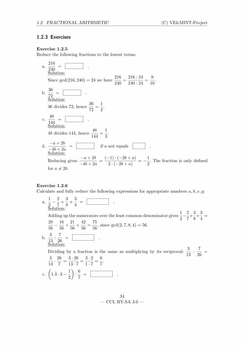
Exercise 1.2.5Reduce the following fractions to the lowest terms:
a.216
240= .
Solution:
Since gcd(216, 240) = 24 we have216
240=
216 : 24
240 : 24=
9
10.
b.36
72= .
Solution:
36 divides 72, hence36
72=
1
2.
c.48
144= .
Solution:
48 divides 144, hence48
144=
1
3.
d.−a+ 2b
−4b+ 2a= if a not equals .
Solution:
Reducing gives−a+ 2b
−4b+ 2a=
(−1) · (−2b+ a)
2 · (−2b+ a)= −1
2. The fraction is only defined
for a 6= 2b.
Exercise 1.2.6Calculate and fully reduce the following expressions for appropriate numbers a, b, x, y:
a.1
2− 2
7+
3
8+
3
4= .
Solution:
Adding up the numerators over the least common denominator gives1
2−2
7+
3
8+
3
4=
28
56− 16
56+
21
56+
42
56=
75
56, since gcd(2, 7, 8, 4) = 56.
b.3
13:
7
26= .
Solution:
Dividing by a fraction is the same as multiplying by its reciprocal:3
13:
7
26=
3
13· 26
7=
3 · 26
13 · 7=
3 · 21 · 7
=6
7.
c.
(1.4 · 3− 1
2
)· 6
7= .
34— CCL BY-SA 3.0 —
1.2. FRACTIONAL ARITHMETIC (C) VE&MINT-Project
Solution:
Converting the decimal expression to a fraction gives
(1.4 · 3− 1
2
)·67
= (1.4 · 18− 3)·1
7= (26− 3) · 1
7=
23
7.
Exercise 1.2.7Convert the following infinite repeating decimal fractions to fractions and fully reducethem:
a. 0.4 = .
b. 0.23 = .
c. 0.1234 = .
d. 0.9 = .
Solution:Using the trick for converting infinite repeating decimal numbers one gets the followingsolutions:
x = 0.4, hence 10x− x = 4 ⇒ 9x = 4 ⇒ x = 49 ,
x = 0.23, hence 100x− x = 23 ⇒ 99x = 23 ⇒ x = 2399 ,
x = 0.1234, hence 100x− x = 12.22 ⇒ 99x = 1222100 ⇒ x = 1222
9900 = 6114950 ,
x = 0.9, hence 10x− x = 9 ⇒ 9x = 9 ⇒ x = 1.
Note for the last part of this exercise, that 1 = 1.000 . . . and 1 = 0.999 . . . = 0.9 are twodecimal representations of the same number.
35— CCL BY-SA 3.0 —
1.3. TRANSFORMATION OF TERMS (C) VE&MINT-Project
1.3 Transformation of terms
1.3.1 Introduction
What exactly are terms?
Info1.3.1
Terms are arithmetic expressions that are combinations of numbers, variables,brackets, and appropriate arithmetic operations.
Terms can be interpreted in two ways:
As functional expressions: If each variable contained in the term is substitutedwith a specific number, the term can be evaluated to a certain value. For example,x+x−1 is a term; once x = 2 is inserted one gets the value 3. The expression 2x−1is a term as well, this term can be transformed into x+x−1, and hence it evaluatesto the same value if x = 2 is inserted. As a symbolic expression, x+x−1 is differentfrom 2x − 1, but as functional expressions they are both the same (equivalent):No matter which value is inserted for x, both terms are always evaluated to thesame value. A term can also be a value on its own, if no variables occur in it. Forexample, 3 · (2 + 4) is a term with the value 18.
As evaluation rules: A term can be interpreted as a type of instruction how tocalculate a new value from given values (inserted into the variables). For example,the term x2 − 1 can be read as “square the value of x and subtract one from theresult”. This is different from the term (x + 1)(x − 1), even if both terms havethe same value. The second term describes the evaluation as “add one to x andmultiply the result with the value, resulting if x is subtracted by one”. The twoterms are mathematically equal. One writes x2 − 1 = (x − 1)(x + 1), but theyrepresent two different ways for calculating the value. Depending on the problemsetting, one of the two terms may be more convenient for solving the problem.
1.3.2 Transformation of Terms
Dealing with terms gets interesting when we investigate the equality of two terms orsimplify complicated terms.
36— CCL BY-SA 3.0 —
1.3. TRANSFORMATION OF TERMS (C) VE&MINT-Project
Info1.3.2
Two terms are equal if they can be transformed into each other by allowed transfor-mations. Complicated terms can be simplified using calculation rules. Note in doingso:
2. If brackets are involved, the distributive property applies:
a · (b± c) = a · b± a · c , (a± b) · c = a · c± b · c .
3. With d 6= 0 we have: (a± b) : d = ad ±
bd .
4. For expressions with nested brackets, first evaluate what’s inside the innermostset of brackets with respect to the calculation rules and then work your waytowards the outermost brackets.
Exercise 1.3.1Remove the brackets from each of the following terms and simplify as far as possible:
Here, for a and b both numbers and whole terms can be inserted.
37— CCL BY-SA 3.0 —
1.3. TRANSFORMATION OF TERMS (C) VE&MINT-Project
Example 1.3.4
A few typical applications of the binomial formulas are:
(1 + 2x)2 = 12 + 2 · 1 · 2x+ (2x)2 = 1 + 4x+ 4x2.
(1 + 2x)(1− 2x) = 12 − (2x)2 = 1− 4x2.
x4 − 1 = (x2 + 1)(x2 − 1) = (x2 + 1)(x + 1)(x − 1), in this transformation itcan be seen, that in the set of real numbers x4 − 1 has only the roots x = 1and x = −1.
Exercise 1.3.2Simplify the following term using the second binomial formula:
(−3x+ 4)(4− 3x) = .
Solution:
(−3x+ 4)(4− 3x) = (4− 3x)(4− 3x) = 16− 24x+ 9x2 .
Example 1.3.5
The binomial formulas can be used to transform quadratic expressions cleverly. Thisis very useful if we want to calculate squares without any aid. For this, the number tobe squared is split into a simple number (usually a power of ten) and the remainder:
Mathematical expressions can be written in different ways that all have their own prosand cons. We distinguish them based on which mathematical operation is to be performedlast. The most common types are the representation as a sum and the representation asa product.
Info1.3.6
For a representation as a product, it is the multiplication that is performed last.Because of the order of operation rule, if any of the factors involves an addition orsubtraction, then having the multiplication be last can only be achieved by enclosingthe factors in brackets. Product is particularly useful for determining cases in whicha term takes the value zero. This happens if and only if one of the factors takes thevalue zero.
For example, the term (x− 1) · (x− 2) is zero if x = 1 or x = 2. For all other values ofx the term takes a non-zero value.
Info1.3.7
For a representation as a sum it is the addition or the subtraction that is perfor-med last. Because of the order of operation rule, terms without brackets are auto-matically in this representation, provided they contain any addition or subtractionat all. From the representation as a sum the asymptotic behaviour of an expressioncan often be deduced. The asymptotic behaviour of a function describes how thefunction behaves if the variable x takes arbitrarily large values. For polynomials,for example, the asymptotic behaviour is determined by the term with the largestexponent.
To change from one representation to another, several methods exist.
Info1.3.8
43— CCL BY-SA 3.0 —
1.3. TRANSFORMATION OF TERMS (C) VE&MINT-Project
Expanding means multiplying each summand of one factor by each summand ofthe other factor and adding up the results. In case of more than two factors, theyshould be multiplied out step by step (only two at a time).
Example 1.3.9
The function f(x) = (x+ 3)(x− 2)(x+ 1) is multiplied out as follows:
f(x) = (x+ 3) · (x− 2) · (x+ 1)
= (x2 + 3x− 2x− 6) · (x+ 1)
= (x2 + x− 6) · (x+ 1)
= x3 + x2 − 6x + x2 + x− 6
= x3 + 2x2 − 5x− 6 .
Exercise 1.3.9Expand the following terms completely and collect like terms. Describe the asymptoticbehaviour of the final expression:
a. f(x) = (3− x)(x+ 1) = .Solution:
(3− x)(x+ 1) = 3x+ 3− x2 − x = 3 + 2x− x2
Description of the asymptotic behaviour:As x approaches ∞ the function f(x) approaches .Solution:If the asymptotic behaviour arises uniquely it can be described for short using thesymbol “lim”:
Solution:Expanding gives f(x) = (3− x)(x+ 1) = −x2 + 2x+ 3. The leading term is −x2. Thusthe graph of the function is a parabola opening downwards with the two asymptotes−∞ for x approaching ±∞:
limx→∞
f(x) = −∞ , limx→−∞
f(x) = −∞ .
In the other parts of this exercise we get by expanding
t · (t+ 1) · (t2 + t+ 1) = t · (t3 + 2t2 + 2t+ 1) = t4 + 2t3 + 2t2 + t .
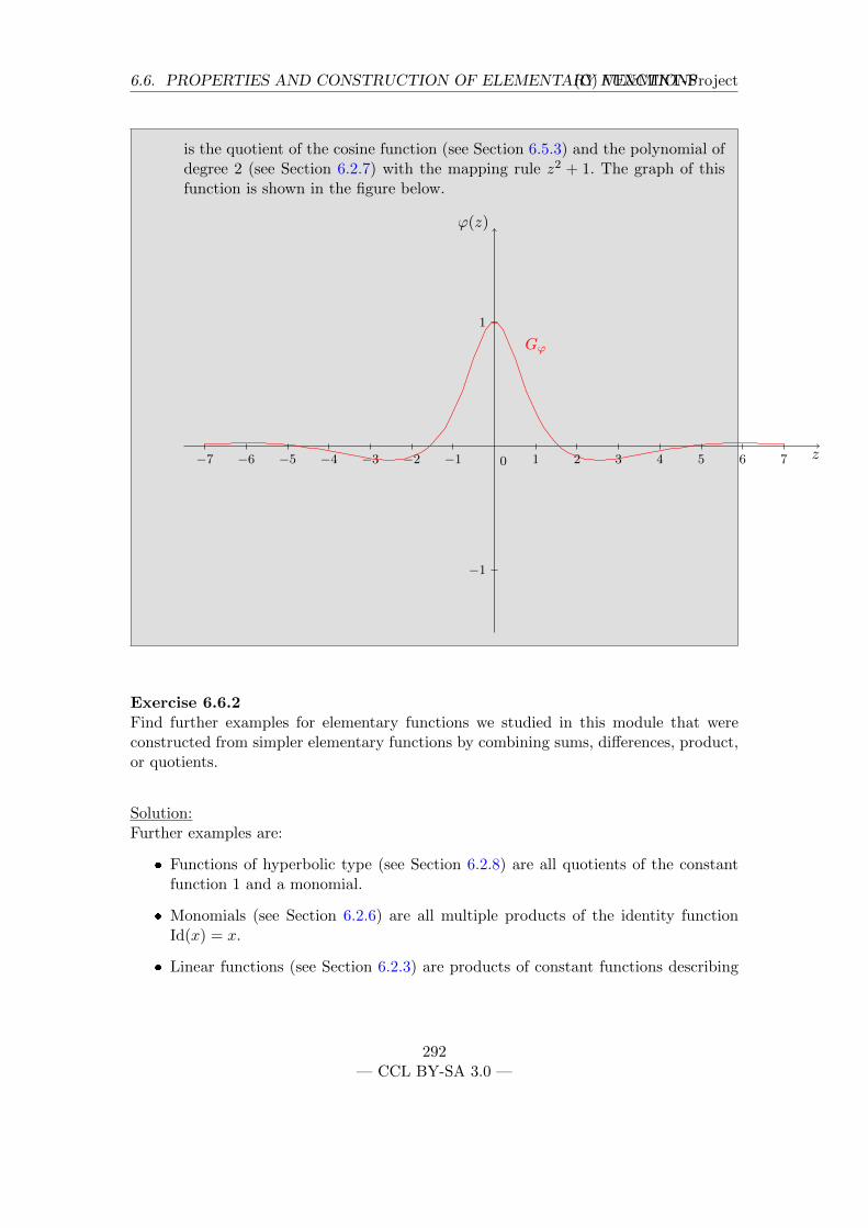
Exercise 1.3.10The following graph corresponds to a polynomial g(x) of degree two:
45— CCL BY-SA 3.0 —
1.3. TRANSFORMATION OF TERMS (C) VE&MINT-Project
−4 −3 −2 −1 1 2 3 4
−20
−10
10
0
Graph of the function g(x).
From the graph, derive the representation of g(x) as a product.
a. The graph has two zeros x1 and x2. Multiplied out the two factors resulting fromthis fact, we get the polynomial f(x) = (x−x1)(x−x2) =.
b. The polynomial f(x) does not correspond to the graph since at x = 0 it takes the
value whereas the graph shows that the function g(x) at x = 0 takes
the value . This difference can be corrected by setting g(x) = c · f(x),
where c = .
c. This finally gives the representation of g(x) as a product: g(x) =.
Solution:The graph shows the zeros x1 = −2 and x2 = 3. Multiplying out the two factors resultingfrom this fact, we get the polynomial f(x) = (x+ 2)(x− 3) = x2 − x− 6. At x = 0, wehave f(0) = −6, but the graph shows g(0) = 12. This difference can be corrected by anadditional factor of −2. In total, we have g(x) = −2x2 + 2x+ 12.
Exercise 1.3.11Fully expand the expression: (a+2b+3c)2 =.
Solution:
46— CCL BY-SA 3.0 —
1.3. TRANSFORMATION OF TERMS (C) VE&MINT-Project
It is simplest to multiply each summand in the first pair of brackets by each summandin the second, finally collecting like terms:
(a+ 2b+ 3c)2 = (a+ 2b+ 3c) · (a+ 2b+ 3c)
= a2 + 2ab+ 3ac+ 2ab+ 4b2 + 6bc+ 3ac+ 6bc+ 9c2
= a2 + 4ab+ 6ac+ 4b2 + 12bc+ 9c2 .
47— CCL BY-SA 3.0 —
1.4. POWERS AND ROOTS (C) VE&MINT-Project
1.4 Powers and Roots
1.4.1 Exponentiation and Roots
The following section deals with expressions of the form as, where a ∈ R. But thequestion is: For which numbers s can this power be reasonably defined?
Powers with positive integer exponents are defined as follows:
Info1.4.1
Let n ∈ N. The n-th power of a number a ∈ R is the n-fold product of the numbera by itself:
an = a · a · a · · · · · a︸ ︷︷ ︸n factors
.
a is called the base and n is called the exponent.
Here, some special cases exist that you should ideally know by heart:
Info1.4.2
For a zero exponent, the value of the power is one, i.e. for example, 40 = 1, also00 = 1. But for a zero base, for n > 0, we have 0n = 0. For base −1, we have
(−1)n = −1 if the exponent is odd , (−1)n = 1 if the exponent is even .
Many powers can be calculated using the calculation rule presented above — but whatabout 2−2?
Info1.4.4
Powers with negative integer exponents are defined by the formula a−n = 1an , n ∈
N, a 6= 0.
Hence 2−2 = 122
= 14 . By analogy, we have (−2)−2 = 1
(−2)2= 1
4 .
Exercise 1.4.1Calculate the values of the following powers.
a. 53 = .
Solution:
53 = 5 · 5 · 5 = 25 · 5 = 125 .
b. (−1)1001 = .
Solution:
(−1)1001 = −1 since the exponent is odd .
c.
(−1
2
)−3
= .
Solution:
(−1
2)−3 =
1
(−12)3
=1
−18
= −8 .
d.((−3)2
)3= .
Solution: ((−3)2
)3= 93 = 729 .
49— CCL BY-SA 3.0 —
1.4. POWERS AND ROOTS (C) VE&MINT-Project
However, even for a rational exponent of the form 1n , n ∈ N, we need to extend this
definition again so that we can calculate 412 , for example. This power can be expressed
as a root as well, namely 412 =√
4 = 2. Generally, we have:
Info1.4.5
Let n ∈ N and a ∈ R with a ≥ 0. The n-th root has the power representationn√a = a
1n .
This leads to one inverse operation of the exponentiation: extracting a root.
Info1.4.6
The n-th root of a number a ∈ R, a ≥ 0, is the number whose n-th power is a:
a1n = n
√a = b =⇒ bn = a .
a is called the base of the root or radicand, and n is called the exponent of theroot or order of the root. We have 1
√a = a, and 2
√a =√a is called the square
root and 3√a is called the cube root of a.
Example 1.4.7
1612 =
2√
16 =√
16 = 4 , 2713 =
3√
27 = 3 .
Info1.4.8
For n ∈ N, a, b ∈ R with a, b ≥ 0 we have the following calculation rules:
1. Two roots with the same exponent are multiplied by multiplying the radi-
50— CCL BY-SA 3.0 —
1.4. POWERS AND ROOTS (C) VE&MINT-Project
cands and extracting the root of the product, leaving the exponent of the rootunchanged:
n√a · n√b =
n√a · b .
2. Two roots with the same exponent are divided by dividing the radicands andextracting the root of the quotient, leaving the exponent of the root unchanged:
n√a
n√b
= n
√a
b, b 6= 0 .
But how can we calculate the number(
10√
4)5
?
Info1.4.9
Let m,n ∈ N and a ∈ R, a ≥ 0.
1. The m-th power of a root is calculated by raising the radicand to the power ofm, leaving the exponent of the root unchanged:(
n√a)m
= n√am = a
mn .
2. The m-th root of a root is calculated by multiplying the exponents of theroots, leaving the radicand unchanged (root of a root).
m
√n√a = m·n√a .
Hence10√
45 = (45)110 = 4
510 = 4
12 =
2√
4 = 2 .
51— CCL BY-SA 3.0 —
1.4. POWERS AND ROOTS (C) VE&MINT-Project
Example 1.4.10
A general power with rational exponent is then calculated as follows:
(1
4
)−23
=3
√(1
4
)−2
=3
√√√√√ 1(1
4
)2 = 3
√√√√ 11
16
=3√
16 =3√
23 · 2 = 23√
2 .
The calculation rules for powers with real base and rational exponent are known asexponent rules. The rules vary depending on whether powers of the same base or thesame exponent are considered.
Exercise 1.4.2Calculate the following roots (here, the result is ):
a.(
5√
3)5
= .
Solution:
(5√
3)5
= (35)15 = 3
5·1
5 = 3 .
b.4√
256 = .
Solution:
4√
256 =(28)1
4 = 22 = 4 .
1.4.2 Calculating using Powers
The following calculation rules allow one to transform and simplify expressions contai-ning powers or roots:
52— CCL BY-SA 3.0 —
1.4. POWERS AND ROOTS (C) VE&MINT-Project
Info1.4.11
For a, b ∈ R, a, b > 0, p, q ∈ Q, the following exponent rules hold:
ap · bp = (a · b)p , ap
bp=(ab
)p, ap · aq = ap+q ,
ap
aq= ap−q , (ap)q = ap·q .
Note that, generally, (ap)q 6= apq, i.e. multiple powers should be bracketed. For example,(
Alternatively, we could have used the exponent rules to calculate (23)4 = 2(3·4) =212 = 4096.
Exercise 1.4.3The following expressions can be simplified using the exponent rules:
a. 33 · 35 · 3−1 = .
Solution:
33 · 35 · 3−1 = 33+5−1 = 37 .
b. 42 · 32 = .
Solution:
42 · 32 = (4 · 3)2 = 122 .
53— CCL BY-SA 3.0 —
1.4. POWERS AND ROOTS (C) VE&MINT-Project
However, when comparing powers and roots, one should take care: not only the values,but also the signs of exponent and base control whether the value of the power is largeor small:
Example 1.4.13
For a positive base and a negative exponent, the value of the power decreases whenincreasing the base:
2−1 =1
2= 0.5
3−1 =1
3= 0.3
4−1 =1
4= 0.25 etc.
For a negative base the sign of the power alternates when increasing the exponent:
(−2)1 = −2
(−2)2 = 4
(−2)3 = −8
(−2)4 = 16 etc.
Extracting the root (or exponentiation with a positive number smaller than one)decreases a base > 1, but increases a base < 1:
Exercise 1.4.4Arrange the following powers in order of size considering the signs of bases and ex-ponents: 23, 2−3, 32, (−3)2, (−3)−2, 3
12 , 2
13 :
< < < < <
= .
Solution:Here, several ways to the correct solution exist. For example, we can raise all terms to the
54— CCL BY-SA 3.0 —
1.4. POWERS AND ROOTS (C) VE&MINT-Project
power of 3 (analogous to the calculation in Example 1.2.13 auf Seite 27). Exponentiationto the power of 3 is allowed since it is an odd number that does not cancel the sign ofthe exponent. In contrast, exponentiation to the power of 2 would cancel all signs suchthat the resulting arrangement would be invalid. We have
(23)3 = 23·3 = 29 = 512
(2−3)3 = 2(−3)·3 = 2−9 =1
512since the exponent is negative
(32)3 = 93 = 81 · 9 = 729
((−3)2)3 = 93 = 729 since the exponent is even
((−3)−2)3 =1
((−3)2)3=
1
729
(312 )3 = 3
32 > 3 (since the exponent is larger than one)
(213 )3 = 2 .
Comparing these values leads to the following arrangement:
(−3)−2 < 2−3 < 213 < 3
12 < 23 < 32 = (−3)2 .
55— CCL BY-SA 3.0 —
1.4. POWERS AND ROOTS (C) VE&MINT-Project
1.4.3 Exercises
Exercise 1.4.5Calculate the following powers:
a.
(−3
5
)4
= .
Solution: (−3
5
)4
=34
54=
81
625.
b.(2−2)−3
= .
Solution: (2−2)−3
= 2(−2)·(−3) = 26 = 64 .
c.
(−1
2
)0
= .
Solution: (−1
2
)0
= 1 .
Exercise 1.4.6Simplify the following expressions using the exponent rules and by reducing the results.You don’t need to evaluate the powers:
a.(−2)7
(−2)5= .
Solution:
(−2)7
(−2)5= (−2)7−5 = (−2)2 .
b. 62 · 3−2 = .
Solution:
62 · 3−2 = 62 ·(
1
3
)2
=
(6 · 1
3
)2
= 22 .
56— CCL BY-SA 3.0 —
1.4. POWERS AND ROOTS (C) VE&MINT-Project
c.643
83= .
Solution:
643
83=
(64
8
)3
= 83 .
d.
(3
4
)13·(
3
4
)23
= .
Solution:
(3
4
)13·(
3
4
)23
=
(3
4
)13 +
23
=3
4.
Exercise 1.4.7Calculate the following roots (here, the result is always an integer):
a.3√
3 · 3√
9 = .
Solution:
3√
3 · 3√
9 =3√
3 · 3 · 3 = 3 .
b.3√
343 = .
Solution:
3√
343 =3√
73 = 7 .
Exercise 1.4.8Simplify the following expressions and write each as a reduced fraction containing nopowers:
a.33 · 63
9 · 23 · 43= .
Solution:
33 · 63
9 · 23 · 43=
34 · 23
23 · 43=
34
43=
81
64.
57— CCL BY-SA 3.0 —
1.4. POWERS AND ROOTS (C) VE&MINT-Project
b. 32 · 9−3 · 276 · 27−2 = .
Solution:
32 · 9−3 · 27−2 · 276 = 32+2·(−3)+3·6−6 = 38 .
58— CCL BY-SA 3.0 —
1.5. FINAL TEST (C) VE&MINT-Project
1.5 Final Test
59— CCL BY-SA 3.0 —
1.5. FINAL TEST (C) VE&MINT-Project
1.5.1 Final Test Module 1
Exercise 1.5.1Check the box in each case to indicate whether the mathematical expressions are equa-tions, inequalities, terms, or numbers (multiple checks are possible):
Mathematical expression Equation Inequality Term Number
1 +1
2− 3(3− 1
2)
5x − x5
x2 <√x
xyz − 1
b2 = 4ac
Exercise 1.5.2
Simplify the compound fraction3 + 3
2112 + 1
4
to a reduced simple fraction:
Exercise 1.5.3Expand the following term completely and collect like terms:
(x− 1) · (x+ 1) · (x− 2) = .
Exercise 1.5.4Apply one of the binomial formulas to transform the term:
a. (x− 3)(x+ 3) = .
b. (x− 1)2 = .
c. (2x+ 4)2 = .
Exercise 1.5.5Rewrite the following expression containing powers and roots as a simple power with arational exponent:
x3
(√x)
3 = .
60— CCL BY-SA 3.0 —
1.5. FINAL TEST (C) VE&MINT-Project
61— CCL BY-SA 3.0 —
2 Equations in one Variable
Module Overview
Equations arise when we require the values of two terms to be equal. If variables occurin at least one of them, an equation can be understood as the task to find out for whichvalues of the variables the left-hand side term and the right-hand side term have thesame value. Simple equations can be solved by applying transformations and solutionformulas from a formulary. For a more sophisticated equation, a case analysis may berequired.
62
2.1. SIMPLE EQUATIONS (C) VE&MINT-Project
2.1 Simple Equations
2.1.1 Introduction
Info2.1.1
An equation is an expression of the form
left-hand side = right-hand side
with mathematical expressions on both sides of the equation. These expressionsgenerally contain variables or unknowns (e.q. x). Depending on the variable valuesan equation is satisfied if both sides of the equation evaluate to the same value. Anequation is not satisfied if the sides of the equation evaluate to different values.
Equations describe relations between expressions or model a problem to be solved. Ingeneral, an equation itself is not true or false. Instead, some variables satisfy the equationand others do not. To test whether the equation is true or false for a single variablevalue this value has to be inserted into the equation. Then, both sides of the equationare evaluated to certain values. The equation is satisfied by an inserted variable value ifthe evaluated values coincide:
Example 2.1.2
The equation 2x− 1 = x2 has the right-hand side x2 and the left-hand side 2x− 1.Inserting x = 1 results in the value 1 on both sides of the equals sign, hence x = 1is a solution of this equation. However, x = 2 is no solution since the left-hand sideof the equation is evaluated to the value 4 while the right-hand side is evaluated tothe value 3.
Info2.1.3
The solution set L of an equation is the set of all numbers satisfying the relation
left-hand side = right-hand side
if inserted into the the equation instead of the variable (e.q. x).
63— CCL BY-SA 3.0 —
2.1. SIMPLE EQUATIONS (C) VE&MINT-Project
Typical problems concerning equations are:
specify the solution set of an equation, i.e. find all variable values satisfying theequation,
transform the equation, in particular, solve an equation for the variables, and
find an equation modelling a problem described textually.
Example 2.1.4
We want to design a savings deposit in such a way that there is a fixed annual return.The bank wants to make sure that when investing over a five-year period, a saverreceives exactly 600 Euros more than when investing over a two-year period.
First, the word problem is translated into an equation with the variable r denotingthe annual return. The resulting equation is 5·r = 2·r+600. It says that five payments(left-hand side of the equation) equal two payments plus 600. (For simplicity, we omitthe unit Euro during calculation.)
We can easily solve this equation can be solved for r by subtracting the term 2r fromboth sides of the equation. The resulting equation reads 3r = 600, and dividing by3 results in the solution r = 200.
Thus, the bank has to offer a return of 200 Euros per year to reach the requiredsavings target.
Info2.1.5
Two equations are said to be equivalent if they have the same solution set.
An equivalent transformation is a special transformation that changes the equa-tion but not its solution set. Important equivalent transformations are
adding/subtracting terms to both sides of the equation,
exchanging both sides of the equation,
transformation of terms on one side of the equation, and
substituting a term for another that is known to always have the same value.
The following transformations are equivalent transformations only if the used termis known to be non-zero (which may depend on the possible values of the variables):
64— CCL BY-SA 3.0 —
2.1. SIMPLE EQUATIONS (C) VE&MINT-Project
multiplying/dividing by a term (this term has to be non-zero),
taking the reciprocal on both sides of the equation (both sides have to benon-zero).
Here, the following notation is used:
equivalent equations are indicated by the symbol ⇔ (which reads: if and only if,i.e. one equation is satisfied if and only if the other equation is satisfied).
under this symbol we put a short description of the transforming operation (or,for solutions with more than one line, the transforming operation is written nextto the transformation).
What matters is that the reader should be able to understand which transformation wascarried out.
Example 2.1.6
This example illustrates two simple equivalent transformations written in a singleline. Even though the symbol ⇔ is two-sided the notation is interpreted in such away that the transformation is applied from left to right:
3x− x2 = 2x− x2 + 1 ⇔+x2
3x = 2x+ 1 ⇔−2x
x = 1 .
The leftmost equation and the rightmost equation are equivalent. On the left wehave the initial equation (corresponding to a certain word problem) and on the rightwe have an equivalent equation showing the solution immediately.
Example 2.1.7
For several complicated transformations, the transformation steps should be writ-ten one under another. In this case we use vertical bars to separate the respectivetransformations from the equations.
65— CCL BY-SA 3.0 —
2.1. SIMPLE EQUATIONS (C) VE&MINT-Project
Start: 12 + t =2t
2t2+ t
∥∥∥∥ − t
⇔ 12 =2t
2t2
∥∥∥∥ sides exchanged
⇔ 2t
2t2= 12
∥∥∥∥ left-hand side transformed
⇔ 1
t= 12
∥∥∥∥ reciprocals taken
⇔ t =1
12.
Here, after the vertical bar both short symbols as, e.g. −t, and textual descriptionsare allowed. Again, what matters is that the reader can understand which transfor-mations were carried out and so can check that everything was done correctly.
2.1.2 Conditions in Transformations
Multiplication, division, and taking reciprocals are equivalent transformations only if thefactors or terms are non-zero. In the last step of example 2.1.7 auf der vorherigen Seite,the reader can see that both sides of the equation are always non-zero. Therefore thetransformation is allowed. If the variables themselves are used in the transformation, weneed to make a note somewhere to remind us that the respective term must be non-zero.The solution at the end of the transformations is then only valid for variable valuessatisfying the transformation conditions. All other values have to be checked separately,typically by inserting the value into the equation:
Example 2.1.8
66— CCL BY-SA 3.0 —
2.1. SIMPLE EQUATIONS (C) VE&MINT-Project
In this example, the necessary transformation conditions are not problematic:
Start: 9x = 81x2
∥∥∥∥ : x, transformation allowed if x 6= 0
⇔ 9 = 81x
∥∥∥∥ : 81 and exchange sides
⇔ x =1
9and this value satisfies the condition x 6= 0 .
The value x = 0, initially rejected by the transformation condition, has to be checkedseparately. The equation 9x = 81x2 is also satisfied for x = 0, hence x = 0 is also asolution of the equation. In set notation, the solution set is L = 0; 1
9.
In any case, values violating a condition have to be checked separately. It may or maynot turn out that they are part of the solution.
Example 2.1.9
Start: x2 − 2x = 2x− 4
∥∥∥∥ factor out on both sides
⇔ x · (x− 2) = 2 · (x− 2) | : (x− 2), transformation only allowed if x 6= 2
⇔ x = 2 .
This value of x violates the condition x 6= 2. Hence, this is possibly no solution.Inserting x = 2 into the initial equation gives 22 − 2 · 2 = 0 on the left-hand sideand also 2 · 2− 4 = 0 on the right-hand side. Hence, x = 2 is indeed a solution, eventhough it violated the transformation condition.
Exercise 2.1.1Find the solution of the equation (x− 2)(x− 3) = x2− 9 by transforming the right-handside using the third binomial formula and then dividing by a common factor.
The solution is x = .
67— CCL BY-SA 3.0 —
2.1. SIMPLE EQUATIONS (C) VE&MINT-Project
Solution:The correct transformation steps including conditions are
Start: (x− 2)(x− 3) = x2 − 9
∥∥∥∥ transformation of the right-hand side
⇔ (x− 2)(x− 3) = (x+ 3)(x− 3)
∥∥∥∥ : (x− 3), transformation allowed if x 6= 3
⇔ x− 2 = x+ 3
∥∥∥∥ − x
⇔ −2 = 3 is a wrong equation.
Importantly, this equation is only wrong for x 6= 3. We have to check x = 3 separately,and indeed x = 3 satisfies the initial equation.
2.1.3 Proportionality and Rule of Three
A relation between two varying quantities that frequently occurs in practice is the pro-portionality. Examples include mass and volume, time and travelled distance or weight(quantity) of a product and its price. Often we are given two example values that standin relation and need to complete another example for which only one value is given. Wewill illustrate this procedure with an example.
Example 2.1.10
5 kg of apples cost 3 Euro. How much do 11 kg of apples cost?
In a first step, we convert the information we have about the price of apples in thefollowing traditional notation, which in this example we could read as “costs”:
5 kg∧= 3 Euro .
In this example, the symbol in the middle can be read as “costs”, but in otherexamples other readings will be required. The key point is that as the value on oneside of the symbol varies, the value on the other will have to vary proportionally.In the second step, we want to scale this proportional relation so as to express itin terms of a unit amount of the quantity for which another value (here: 11 kg) isgiven. So we multiply both sides by 1/5 and get:
1 kg∧=
1
5· 3 Euro = 0.6 Euro .
68— CCL BY-SA 3.0 —
2.1. SIMPLE EQUATIONS (C) VE&MINT-Project
In the third and final step, we multiply both sides by the number of units specifiedin the problem, which in our example is 11:
11 kg∧= 11 · 0.6 Euro = 6.6 Euro .
The required price for 11 kg of apples is therefore 6.60 Euro.
We have derived the required relation by deriving a relation for one unit of a quantityfrom the initial relation. The procedure demonstrated here is called the rule of threeand is taught in great detail in the schools of some countries such as Germany andFrance.
The same problem can also be solved by introducing a proportionality factor. Again, weconsider the example above.
Example 2.1.11
The price P is proportional to the mass m. Hence, there exists a constant k with
P = km .
Since this relation also holds for the given values m0 = 5 kg and P0 = 3 Euro itfollows
P0 = km0
∥∥∥ multiplying by1
m0
⇐⇒ P0
m0= k ;
hence in this case
k =3
5= 0.6 ,
taken in the unit of Euro per kg. (As a scientist you would correctly write k =0.6 Euro/kg, since proportionality factors generally carry a dimensional unit.) Usingm1 = 11 kg, one obtains finally
P1 = km1 = 0.6 · 11 = 6.6 (Euro)
which is the same result as for using the rule of three (see previous example).
69— CCL BY-SA 3.0 —
2.1. SIMPLE EQUATIONS (C) VE&MINT-Project
Exercise 2.1.2A car takes 9 minutes to travel a distance of 6 km.
a. Which distance s the car travels within 15 minutes?
The solution is s15 = km.
b. The proportionality factor between travelled distance s and travelling time t is thevelocity v of the car.
The velocity is v = km/ h.
Solution:¿From the given values we know that the car travels 6
9 km = 23 km within one minute
and therefore 15 · 23 km = 10 km within 15 minutes.
So, the velocity is
v =10 km
15 min=
10 km
(1/4) h= 40
km
h.
2.1.4 Solving linear Equations
Info2.1.12
A linear equation is an equation in which only multiples of variables and constantsoccur.
For a linear equation in one variable (here the variable x) one of the following threestatements holds:
The equation has no solution.
The equation has a single solution.
Every value of x is a solution of the equation.
These three cases are distinguished by means of the transformation steps:
If the transformation ends up in a statement that is wrong for all x (e.g. 1 = 0)then the equation is unsolvable.
70— CCL BY-SA 3.0 —
2.1. SIMPLE EQUATIONS (C) VE&MINT-Project
If the transformation ends up in a statement that is true for all x (e.g. 1 = 1) thenthe equation is solvable for all values of x.
Otherwise, the equation can be solved, i.e. it can be transformed into the equationx = value which is the solution.
Set notation2.1.13
Using set notation (with L as the conventional symbol for the solution set) thesecases can be expressed as follows:
L = or L = ∅ if there is no solution,
L = value if there is a single solution,
L = R if all real numbers x are a solution.
Example 2.1.14
The linear equation 3x + 2 = 2x − 1 has one solution. This solution is obtained byequivalent transformations:
3x+ 2 = 2x− 1 ⇔−2x
x+ 2 = −1 ⇔−2
x = −3 .
Hence, x = −3 is the only solution.
Example 2.1.15
The linear equation 3x+ 3 = 9x+ 9 has the solution:
3x+ 3 = 9x+ 9 ⇔:(x+1)
3 = 9 .
This statement is wrong. Hence, for all x 6= −1 (transformation condition) theequation is wrong. Inserting x = −1 satisfies the equation, and so the only solutionis x = −1.
Alternatively, the equation could have been transformed as follows:
3x+ 3 = 9x+ 9 ⇔−3x−9
−6 = 6x ⇔ x = −1 .
71— CCL BY-SA 3.0 —
2.1. SIMPLE EQUATIONS (C) VE&MINT-Project
Exercise 2.1.3Transform the following linear equations and specify their solution sets:
a. The equation x− 1 = 1− x has the solution set L = ,
b. The equation 4x− 2 = 2x+ 2 has the solution set L = ,
c. The equation 2x− 6 = 2x− 10 has the solution set L = .
Solution:The first equation can be transformed into 2x = 2 or x = 1, respectively, so the solutionset is L = 1. The second equation can be transformed into 2x = 4 and the solutionset is L = 2. The third equation can be transformed into −6 = −10 which is a falsestatement, hence L = .
Exercise 2.1.4Find the solution of the general linear equation ax = b with a and b being real numbers.Specify the values of a and b for which the following three cases occur:
Every value of x is a solution (L = R) if a = and b = 0.
There is no solution (L = ∅) if a = and b 6= .
Otherwise, there is a single solution, namely x = .
Solution:Every value of x is a solution (L = R) if a = 0 and b = 0. There is no solution (L = ∅)if a = 0 and b 6= 0. Otherwise, there is only one solution, namely x = b
a .
2.1.5 Solving quadratic Equations
Info2.1.16
A quadratic equation is an equation of the form ax2 + bx+ c = 0 with a 6= 0, or,in reduced form, x2 + px+ q = 0. This form is obtained by dividing the equation bya.
For a quadratic equation in one variable (here the variable x) one of the followingthree statements holds:
72— CCL BY-SA 3.0 —
2.1. SIMPLE EQUATIONS (C) VE&MINT-Project
The quadratic equation has no solution: L = .
The quadratic equation has a single solution L = x1.
The quadratic equation has two different solutions L = x1;x2.
The solutions are obtained by applying quadratic solution formulas.
Info2.1.17
The pq formula for solving the equation x2 + px+ q = 0 reads
x1,2 = −p2±√
1
4p2 − q .
Here, the equation has
no (real) solution if 14p
2 − q < 0 (taking the square root is not allowed),
a single solution x1 = −p2 if 1
4p2 = q and the square root is zero,
two different solutions if the square root is a positive number.
The expression D := 14p
2 − q underneath the square root considered above is calledthe discriminant.
The solution of a quadratic equation is often described by an alternative formula:
Info2.1.18
For the equation ax2 + bx+ c = 0 with a 6= 0 the abc formula reads
x1,2 =−b±
√b2 − 4ac
2a.
Here, the equation has
no (real) solution if b2 − 4ac < 0 (the square root of a negative number isundefined within the range of real numbers),
73— CCL BY-SA 3.0 —
2.1. SIMPLE EQUATIONS (C) VE&MINT-Project
a single solution x1 = − b2a if b2 = 4ac and the square root is zero,
two different solutions if the square root is a positive number.
Again, the expression D := b2− 4ac underneath the square root considered above iscalled the discriminant.
Both formulas result in the same solutions. The pq formula is easier to learn, but is onlyapplicable if a, the coefficient of the quadratic term, is 1. Otherwise we must divide bothsides of the equation by a.
In terms of the pq formula, the three different cases correspond to three possibiliesfor the number of intersection points that the graph of a shifted standard parabolaf(x) = x2 + px+ q may have with the x axis.
−3 −2 −1 1 2 3
−3
−2
−1
1
2
3
0 −3 −2 −1 1 2 3
−3
−2
−1
1
2
3
0 −3 −2 −1 1 2 3
−3
−2
−1
1
2
3
0
Three cases: no intersection point, one intersection point, two intersection points withthe x axis.
Example 2.1.19
The quadratic equation x2−x+1 = 0 has no solution since the discriminant 14p
2−q =−3
4 within the pq formula is negative. In contrast, the equation x2 − x − 1 = 0 hastwo solutions
x1 =1
2+
√1
4+ 1 =
1
2(1 +
√5) ,
x2 =1
2−√
1
4+ 1 =
1
2(1−
√5) .
74— CCL BY-SA 3.0 —
2.1. SIMPLE EQUATIONS (C) VE&MINT-Project
Info2.1.20
The function expression of a parabola has vertex form if the function has the formf(x) = a · (x− s)2−d with a 6= 0. In this case, (s;−d) is the vertex of the parabola.The corresponding quadratic equation for f(x) = 0 then reads a · (x− s)2 = d.
Dividing this equation by a one obtains the equivalent quadratic equation (x−s)2 =da . Since the left-hand side is a square of a real number, only solutions exist if and
only if the right-hand side is non-negative as well, i.e. da ≥ 0. By taking the square
root, taking the two possible signs into account, one obtains x− s = ±√
da .
So, for da > 0 two solutions of the equation exist:
x1 = s−√d
a, x2 = s+
√d
a;
they are symmetric to the x coordinate s of the vertex. For d = 0, only one solutionexists.
The sign of a determines whether the function expression describes a parabola ope-ning upwards or downwards.
The quadratic equation has only one single solution s if it can be transformed into theform (x− s)2 = 0.
Info2.1.21
Any quadratic equation can be transformed (after collecting terms on the left-handside and normalisation, if necessary) to vertex form by completing the square.For this, a constant is added to both sides of the equation such that on the left-handside we have a term of the form x2 ± 2sx+ s2 to which the first or second binomialformula can be applied.
Example 2.1.22
75— CCL BY-SA 3.0 —
2.1. SIMPLE EQUATIONS (C) VE&MINT-Project
Adding the constant 2 transforms the equation x2 − 4x + 2 = 0 into the formx2−4x+4 = 2 or into the form (x−2)2 = 2, respectively. From this, the two solutionsx1 = 2−
√2 and 2+
√2 can be seen immediately. In contrast, the quadratic equation
x2 + x = −2 has no solution since completing the square results in x2 + x+ 14 = −7
4or (x+ 1
2)2 = −74 , respectively, where the right-hand side is negative for a = 1.
Exercise 2.1.5Find the solutions of the following quadratic equations by completing the square aftercollecting terms on the left-hand side and normalisation (i.e. selecting a = 1):
a. x2 = 8x− 1 has the vertex form = .
The solution set is L = .
b. x2 = 2x+ 2 + 2x2 has the vertex form = .
The solution set is L = .
c. x2 − 6x+ 18 = −x2 + 6x has the vertex form =.The solution set is L = .
Solution:The transformations are for the first equation
x2 = 8x− 1
⇔ x2 − 8x+ 1 = 0
⇔ x2 − 8x+ 16 = 15
⇔ (x− 4)2 = 15
L = 4−√
15; 4 +√
15
and for the second equation
x2 = 2x+ 2 + 2x2
⇔ x2 + 2x+ 2 = 0
⇔ x2 + 2x+ 1 = −1
⇔ (x+ 1)2 = −1
L =
76— CCL BY-SA 3.0 —
2.1. SIMPLE EQUATIONS (C) VE&MINT-Project
and for the third equation
x2 − 6x+ 18 = −x2 + 6x
⇔ 2x2 − 12x+ 18 = 0
⇔ x2 − 6x+ 9 = 0
⇔ (x− 3)2 = 0
L = 3 .
77— CCL BY-SA 3.0 —
2.2. ABSOLUTE VALUE EQUATIONS (C) VE&MINT-Project
2.2 Absolute Value Equations
2.2.1 Introduction
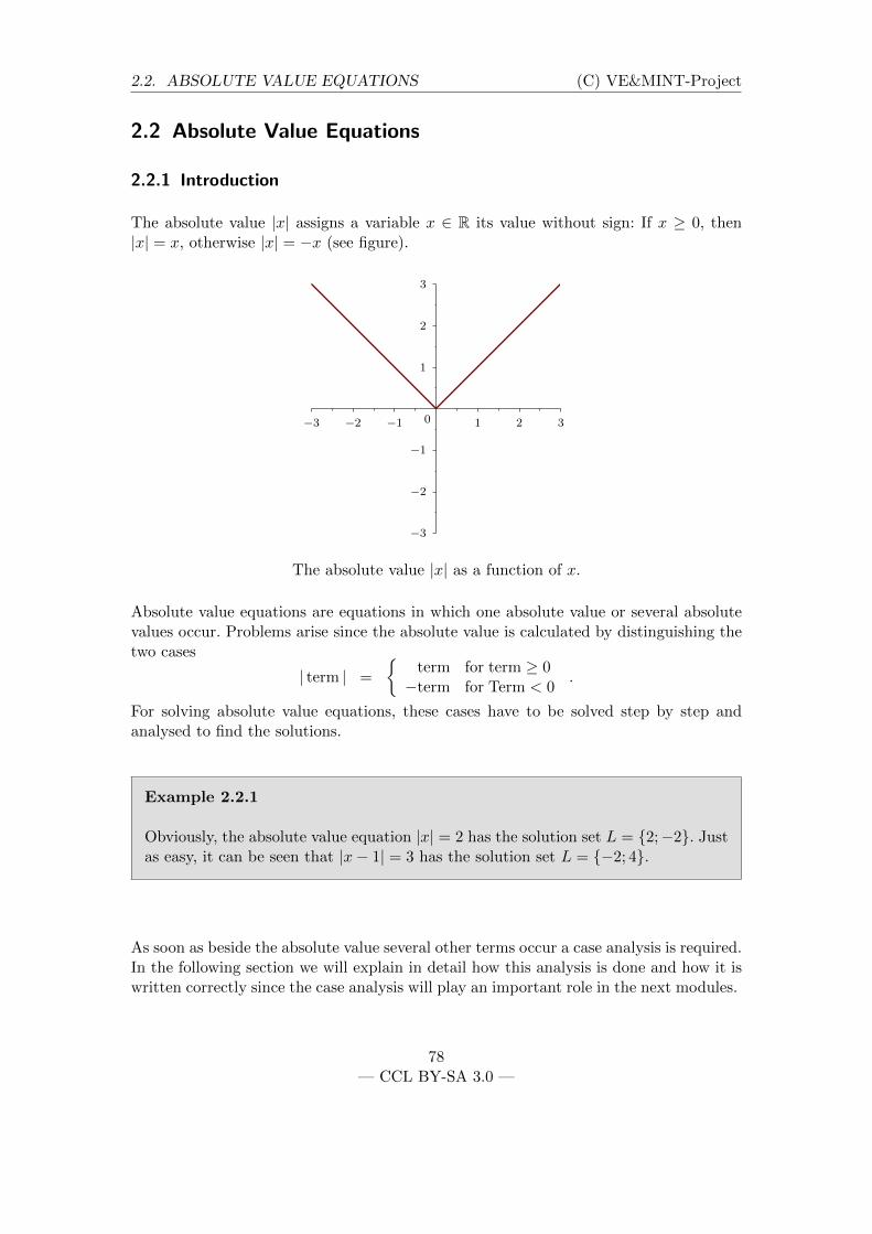
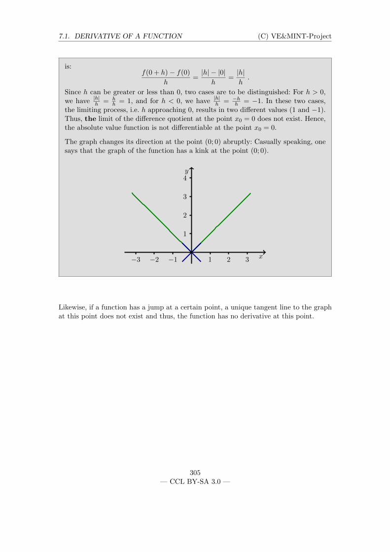
The absolute value |x| assigns a variable x ∈ R its value without sign: If x ≥ 0, then|x| = x, otherwise |x| = −x (see figure).
−3 −2 −1 1 2 3
−3
−2
−1
1
2
3
0
The absolute value |x| as a function of x.
Absolute value equations are equations in which one absolute value or several absolutevalues occur. Problems arise since the absolute value is calculated by distinguishing thetwo cases
| term | =
term for term ≥ 0−term for Term < 0
.
For solving absolute value equations, these cases have to be solved step by step andanalysed to find the solutions.
Example 2.2.1
Obviously, the absolute value equation |x| = 2 has the solution set L = 2;−2. Justas easy, it can be seen that |x− 1| = 3 has the solution set L = −2; 4.
As soon as beside the absolute value several other terms occur a case analysis is required.In the following section we will explain in detail how this analysis is done and how it iswritten correctly since the case analysis will play an important role in the next modules.
78— CCL BY-SA 3.0 —
2.2. ABSOLUTE VALUE EQUATIONS (C) VE&MINT-Project
2.2.2 Carry out a Case Analysis
Info2.2.2
To solve an absolute value equation two cases are distinguished:
For all values of x for which the absolute value term is non-negative the absolutevalue can be omitted or replaced by simple brackets, respectively.
For all values of x for which the absolute value term is negative the term isbracketed and negated.
Then, the solution sets from the case analyses will be restricted to satisfy the caseconditions. Only if this procedure is finished for all cases, the solution subsets willbe merged to the solution set of the initial equation.
For solving absolute value equations it is important to write down the solution stepscorrectly and to distinguish the cases clearly.
The following video demonstrates a detailed written solution of the absolute value equa-tion |2x− 4| = 6 by case analysis.
(Video cannot be played)
Video 1: Carry out a case analysis.
The case analysis presented in the video can be written briefly as follows:
|2x− 4| =
2x− 4 for x ≥ 2−2x+ 4 for x < 2
=
2x− 4 for x ≥ 2−2x+ 4 otherwise
.
Exercise 2.2.1Describe the values of the expression 2 · |x− 4| by a case analysis:
2 · |x− 4| = .
Solution:
79— CCL BY-SA 3.0 —
2.2. ABSOLUTE VALUE EQUATIONS (C) VE&MINT-Project
2 · |x− 4| =
2x− 8 for x ≥ 4−2x+ 8 for x < 4
Exercise 2.2.2Reproduce the steps shown in the video 2.2.2 auf der vorherigen Seite to solve theabsolute value equation |6 + 3x| = 12.
The case analysis reads shortly |6 + 3x| = .Solution:
|6 + 3x| =
6 + 3x for x ≥ −2−6− 3x for x < −2
Finding the solution for each case and checking the case conditions leads to the solutionset L = for the equation |6 + 3x| = 12.
Solution:
L = −6; 2
You can practise the stepwise solution of absolute value equations within the followingexercise.
In the online version, exercises from an exercise list will be shown here
2.2.3 Mixed Equations
Info2.2.3
If an equation contains both absolute values and other expressions, the case analysishas to be done according to the absolute value terms and applied only to these.
80— CCL BY-SA 3.0 —
2.2. ABSOLUTE VALUE EQUATIONS (C) VE&MINT-Project
Finally, keep in mind to cross-check the solution sets you found with the case conditions.
Example 2.2.4
Solve the equation |x− 1|+ x2 = 1. Here, the case analysis is as follows:
For x ≥ 1, the absolute value bars can be replaced by normal brackets whichresults in the quadratic equation (x− 1) + x2 = 1 that is transformed into theequation x2 + x− 2 = 0. Using the pq formula we get the two solutions
x1 = −1
2−√
9
4= −2 ,
x2 = −1
2+
√9
4= 1
of which only x2 satisfies the case condition.
For x < 1, one obtains the quadratic equation −(x − 1) + x2 = 1 that istransformed into the equation x2 − x = 0 or x · (x− 1) = 0, respectively. Theproduct representation indicates the two solutions x3 = 0 and x4 = 1. Becauseof the case condition only x3 = 0 is a solution of the initial equation.
So, altogether L = 0; 1 is the solution set of the initial equation.
Exercise 2.2.3Find the solution set of the mixed equation |x− 3| · x = 9.
a. If x is in the interval the absolute value term is non-negative.
One obtains the quadratic equation = 0.
The solution set is .
Only the solution satisfies the case condition.
b. If x is in the interval the absolute value term is negative.
One obtains the normalised quadratic equation = 0.
The solution set is .
So, altogether the solution set is L = .
Solution:If x is in the interval [3;∞[ the absolute value term is non-negative and one obtains the
quadratic equation x2− 3x− 9 = 0 with the solution set L = 32 −
√454 ; 3
2 +√
454 . Only
81— CCL BY-SA 3.0 —
2.2. ABSOLUTE VALUE EQUATIONS (C) VE&MINT-Project
the larger solution 32 +
√454 satisfies the condition x ≥ 3. This can also be seen without
any calculator by estimating√
454 ≥
√364 = 3. In contrast, if x is in the interval ]−∞; 3[
the absolute value term is negative. One obtains the normalised quadratic equationx2 − 3x + 9 = 0. Because of 1
4p2 − q < 0 in the pq formula this equation is unsolvable.
Hence, the initial equation has only one solution 32 +
√454 .
Exercise 2.2.4Find the solutions of the mixed absolute value equation 3|2x+1| = |x−5| by visualisingthe different cases on the number line and finally solving the equation by case analysis.First, visualise the case analysis for each absolute value.
The solution set is .
Solution:Visualising the different cases for the expressions |2x + 1| and |x − 5| above each otherindicates all cases to be distinguished:
−4 0 4 8 12
Case (1) Case (2) Case (3)
−12
5
x− 5 < 0 x− 5 > 0
5
2x+ 1 < 0 2x+ 1 > 0
−12
−4 0 4 8 12
Case (1) Case (2) Case (3)
−12
5
x− 5 < 0 x− 5 > 0
5
2x+ 1 < 0 2x+ 1 > 0
−12
−4 0 4 8 12
Case (1) Case (2) Case (3)
−12
5
x− 5 < 0 x− 5 > 0
5
2x+ 1 < 0 2x+ 1 > 0
−12
Illustration of the three cases
According to the figure above the following three cases have to be distinguished:
Case (1): For x < −12 both terms in the absolute value terms are negative.
Case (2): For −12 ≤ x < 5 the term in the second absolute value term is negative
but the term in the first one is not.
82— CCL BY-SA 3.0 —
2.2. ABSOLUTE VALUE EQUATIONS (C) VE&MINT-Project
Case (3): For 5 ≤ x both terms in the absolute value terms are non-negative.
Obviously, there is no x for which the first term is negative and the second termis non-negative.
So, the solutions can be summarised:
In case (1), both absolute values reverse the sign of the terms:3|2x+ 1| = |x− 5| ⇔ 3(−(2x+ 1)) = −(x− 5).This equation has the solution x = −8
5 satisfying the case condition.
In case (2), only the second absolute value reverses the sign of the term:3|2x+ 1| = |x− 5| ⇔ 3(2x+ 1) = −(x− 5).This equation has the solution x = 2
7 satisfying the case condition.
In case (3), the absolute value bars in both terms can be omitted (replaced bynormal brackets):3|2x+ 1| = |x− 5| ⇔ 3(2x+ 1) = (x− 5).This equation has the solution x = −8
5 , but this solution does not satisfy the casecondition. Thus, it will be discarded within its case analysis.
Therefore, the solution set is −85 ; 2
7.
83— CCL BY-SA 3.0 —
2.3. FINAL TEST (C) VE&MINT-Project
2.3 Final Test
84— CCL BY-SA 3.0 —
2.3. FINAL TEST (C) VE&MINT-Project
2.3.1 Final Test Module 2
Exercise 2.3.1Find an absolute value term describing the following graph of a function as simply aspossible:
−4 −2 2 4
−4
−2
2
4
Graph of the function f(x).
Answer: f(x) = .
Exercise 2.3.2Solve the following equations:
a. |2x− 3| = 8 has the solution set .
b. |x− 2| · x = 0 has the solution set .
85— CCL BY-SA 3.0 —
2.3. FINAL TEST (C) VE&MINT-Project
Exercise 2.3.3A camera has a resolution of 6 megapixels, i.e. – for convenience – 6 million pixels andproduces images in format 2 : 3. Which size has a quadratic pixel on a print-out offormat (60 cm)× (40 cm)? Specify the side length of a pixel in millimetre.
Answer: (without the unit mm).
Exercise 2.3.4Find the solution set of the mixed equation |x− 1| · (x+ 1) = 3.
Answer: L = .
86— CCL BY-SA 3.0 —
3 Inequalities in one Variable
Module Overview
An inequality arises when we relate two terms using one of the comparators≤,<,≥, or>.Simple inequalities usually have intervals as their solution sets. But solving inequalitiesis often more difficult than solving equations. Hence, specific types of inequalities willbe explained in more detail.
87
3.1. INEQUALITIES AND THEIR SOLUTION SETS (C) VE&MINT-Project
3.1 Inequalities and their Solution Sets
3.1.1 Introduction
Info3.1.1
If two numbers are related by one of the comparators ≤, <, ≥, or >, a statementis generated that can be true or false depending on the numbers:
a < b (reads: “a is strictly less than b” or simply “a is less than b”) is true ifthe number a is less than and not equal to b.
a ≤ b (reads: “a is less than b”) is true if a is less than or equal to b.
a > b (reads: “a is strictly greater than b” or simply “a is greater than b”) istrue if the number a is greater and not equal to b.
a ≥ b (reads: “a is greater than b”) is true if the number a is greater than orequal to b.
The comparators describe how the given values are related to each other on the numberline: a < b means that a is to the left of b on the number line.
Example 3.1.2
The statements 2 < 4, −12 ≤ 2, 4 > 1, and 3 ≥ 3 are true, but the statements2 <√
2 and 3 > 3 are false.
−1 0 1 2 3 4 R
On the number line, the number 2 is to the left of the number 4, thus 2 < 4.
Here, a < b means the same as b > a, likewise a ≤ b means the same as b ≥ a. But itshould be noted that the opposite of the statement a < b is the statement a ≥ b and nota > b. If terms with a variable occur in an inequality, the problem is to find the numberrange of the variable such that the inequality is true.
88— CCL BY-SA 3.0 —
3.1. INEQUALITIES AND THEIR SOLUTION SETS (C) VE&MINT-Project
3.1.2 Solving simple Inequalities
If the variable occurs isolated in the inequality, the solution set is an interval, see alsoinfo box 1.1.5 auf Seite 9:
Info3.1.3
The solved inequalities have the following intervals as their solution sets:
x < a has the solution set ]−∞; a[ , i.e. all x less than a.
x ≤ a has the solution set ]−∞; a], i.e. all x less than or equal to a.
x > a has the solution set ]a;∞[ , i.e. all x greater than a.
x ≥ a has the solution set [a;∞[ , i.e. all x greater than or equal to a.
Here, x is the variable and a is a specific value. If the variable does not occur inthe inequality anymore, the solution set is either R = ]−∞;∞[ if the inequality issatisfied, or the empty set if the inequality is not satisfied.
The symbol ∞ means infinity. A finite interval has the form ]a; b[ which reads “allnumbers between a and b”. If the interval is bounded only on one side, we can write thesymbol ∞ (right-hand side) or −∞ (left-hand side) as the other bound.
As in the case of equations, one tries to find a solved inequality by applying transfor-mations that do not change the solution set. The solution set can be read off from thesolved inequality.
Info3.1.4
To obtain a solved inequality from an unsolved inequality the following equivalenttransformations are allowed:
adding a constant to both sides of the inequality: a < b is equivalent to a+ c <b+ c.
multiplying both sides of the inequality by a positive constant: a < b is equi-valent to a · c < b · c if c > 0.
multiplying both sides of the inequality by a negative constant and inverting
89— CCL BY-SA 3.0 —
3.1. INEQUALITIES AND THEIR SOLUTION SETS (C) VE&MINT-Project
the comparator: a < b is equivalent to a · c > b · c if c < 0.
Example 3.1.5
The inequality −34x−
12 < 2 is solved stepwise by the above transformations:
−3
4x− 1
2< 2
∥∥∥∥ +1
2
⇔ −3
4x < 2 +
1
2
∥∥∥∥ ·(−4
3
)⇔ x > −4
3
(2 +
1
2
) ∥∥∥∥ simplifying
⇔ x > −20
6= −10
3.
So, the initial inequality has the solution set]−10
3 ;∞[
. Importantly, multiplyingthe inequality by the negative number −4
3 inverts the comparator.
Exercise 3.1.1Are the following inequalities true or false?
12 > 1− 1
3
a2 ≥ 2ab− b2 (where a and b are unknown numbers)12 <
23 <
34
Let a < b, then also a2 < b2.
Solution:The first inequality can be simplified to 1
2 >23 , which, after multiplying by 6, is equivalent
to 3 > 4. This statement is false. The second inequality can be simplified by collectingall numbers on the left-hand side: a2 − 2ab+ b2 ≥ 0. Since a2 − 2ab+ b2 = (a− b)2, thisstatement is true for all a and b. Multiplying the third chain of inequalities by the leastcommon denominator 12 results in the chain of inequalities 6 < 8 < 9. This statementis true. In contrast, the last statement is false, since for example, for a = −1 and b = 1,the term a2 = 1 is not less than b2 = 1. Taking the square of terms is not an equivalenttransformation.
Exercise 3.1.2
90— CCL BY-SA 3.0 —
3.1. INEQUALITIES AND THEIR SOLUTION SETS (C) VE&MINT-Project
Find the solution sets of the following inequalities.
a. 2x+ 1 > 3x− 1 has the solution interval L = .
b. −3x− 12 ≤ x+ 1
2 has the solution interval L = .
c. x− 12 ≤ x+ 1
2 has the solution interval L = .
Solution:Transformation of the first inequality results in
2x+ 1 > 3x− 1
∥∥∥∥ + 1
⇔ 2x+ 2 > 3x
∥∥∥∥ − 2x
⇔ 2 > x
and hence the solution interval is L = ]−∞; 2[ . Transformation of the second inequalityresults in
−3x− 1
2≤ x+
1
2
∥∥∥∥ + 3x− 1
2
⇔ −1 ≤ 4x
∥∥∥∥ · 1
4
⇔ −1
4≤ x
and hence L =[−1
4 ;∞[
. Transformation of the third inequality results in
x− 1
2≤ x+
1
2
∥∥∥∥ − x
⇔ −1
2≤ 1
2.
This statement does not depend on x ∈ R and is always true, thus the solution set isL = R = ]−∞;∞[ .
Info3.1.6
An inequality in one variable x is linear if on both sides of the inequality onlymultiples of x and constants occur. Each linear inequality can be transformed intoa solved inequality by one of the equivalent transformations described in the infobox 3.1.3 auf Seite 84.
91— CCL BY-SA 3.0 —
3.1. INEQUALITIES AND THEIR SOLUTION SETS (C) VE&MINT-Project
3.1.3 Specific Transformations
The following equivalent transformations are useful if the variable occurs in the denomi-nator of an expression. But they can only be applied under certain restrictions:
Info3.1.7
Under the restriction that none of the occurring denominators is zero (the correspon-ding variable values are never solutions) and the fractions on both sides have thesame sign, the reciprocal can be taken on both sides of the inequality while invertingthe comparator.
Example 3.1.8
For example, the inequality 12x ≤
13x is equivalent to 2x ≥ 3x (comparator inverted)
as long as x 6= 0. The new inequality has the solution set ]−∞; 0]. However, sincethe value x = 0 was excluded (and does not belong to the domain of the initialinequality either) the solution set of 1
2x ≤1
3x is L = ]−∞; 0[ .
Exercise 3.1.3Find the solution sets of the following inequalities.
a. 1x ≥
13 has the solution set L = .
b. 1x <
1√x
has the solution set L = .
Solution:For the first inequality, the value x = 0 is not in the domain, hence this value is excluded.For x > 0, taking the reciprocal while inverting the comparator is allowed and results inx ≤ 3. Together with the condition above the solution interval is L = ]0; 3]. For x < 0the reciprocal rule cannot be applied. However, it can be seen, even without any rule,that none of the values x < 0 can be a solution, since then 1
x is negative as well and notgreater than or equal to 1
3 .
The domain of the second inequality is ]0;∞[, since only for these values of x taking thesquare root is defined and only for x 6= 0 the denominators are non-zero. On the domain,taking the reciprocal while inverting the comparator is allowed and results in x >
√x.
Since√x > 0, the inequality can be divided by
√x resulting in
√x > 1. This inequality
92— CCL BY-SA 3.0 —
3.1. INEQUALITIES AND THEIR SOLUTION SETS (C) VE&MINT-Project
has the solution set L = ]1;∞[ which occurs also in the domain.
Please note for the last part of the exercise:
Info3.1.9
Taking the square on both sides of an inequality is not an equivalent transformationand possibly does change the solution set.
For example, x = −2 is no solution of x >√x, but indeed a solution of x2 > x. However,
this transformation can be applied if the case analysis for the transformation is carriedout correctly and the domain of the initial inequality is taken into account. This methodis described in more detail in the next section.
93— CCL BY-SA 3.0 —
3.2. TRANSFORMATION OF INEQUALITIES (C) VE&MINT-Project
3.2 Transformation of Inequalities
3.2.1 Transformation with Case Analysis
The simple linear transformations described in the previous section are equivalent trans-formations. They do not change the solution set of the corresponding inequality. Fornonlinear inequalities, advanced solution methods are required. Usually, these methodsneed a case analysis depending on the sign. This is because, in contrast to the situationfor equations described in Module 2, now also the comparator can be inverted whenperforming transformations.
Info3.2.1
If an inequality is multiplied by a term in which the variable x occurs, a case analysisis required and for each case the transformation has to be considered separately:
For those values of x, for which the multiplied term is positive, the comparatorof the inequality is unchanged.
For those values of x, for which the multiplied term is negative, the comparatorof the inequality is inverted.
The case that the multiplied term is zero has to be excluded during the trans-formation and has to be considered separately, if necessary.
The solution sets found in the individual cases have to be checked with re-spect to the case conditions as described for the solution of absolute valueequations.
In contrast, adding terms in which the variable occurs, does not require a case analysis.Usually, transformations involving case analyses are mandatory if the variable occurs inthe denominator or in a composite term.
Example 3.2.2
The inequality 12x ≤ 1 can be simplified by multiplying both sides of the inequality
94— CCL BY-SA 3.0 —
3.2. TRANSFORMATION OF INEQUALITIES (C) VE&MINT-Project
by the term 2x:
Under the condition x > 0 this results in the new inequality 1 ≤ 2x. It has thesolution set L1 =
[12 ;∞
[. The condition x > 0 is satisfied by all elements of
the solution set.
Under the condition x < 0 this results in the new inequality 1 ≥ 2x. It hasthe solution set
]−∞; 1
2
]. Because of the additional condition x < 0 only the
elements of the set L2 = ]−∞; 0[ are solutions.
The single case x = 0 is no solution since this value is not in the domain of theinequality. In this case multiplying the inequality by x is not allowed.
So, altogether one obtains the union set L = L1 ∪ L2 = R \[0; 1
2
[as solution set:
−1 0 1 2 3 4 R
As in Module 2 the following statement holds for the solution set.
Info3.2.3
The cases have to be chosen such that all elements of the domain of the inequalityare covered. For the solution set in an individual case, it has to be checked that thesolution set satisfies the corresponding case condition. For any case, the resultingsolution set has to be reduced to the solution subset satisfying the case condition.The union of the solution sets for the individual cases is the solution set of the initialinequality.
95— CCL BY-SA 3.0 —
3.2. TRANSFORMATION OF INEQUALITIES (C) VE&MINT-Project
3.2.2 Exercises
If the inequality is multiplied by a composite term, we must investigate precisely forwhich values of x the case analysis must be done:
Exercise 3.2.1Find the solution set of the inequality 1
4−2x < 3. The domain of the inequality is D =R \ 2 since only for these values of x the denominator is non-zero. If the inequality ismultiplied by the term 4− 2x, three cases have to be distinguished. Fill in the blanks inthe following text accordingly:
a. On the interval the term is positive, the comparator remains
unchanged, and the new inequality reads 1 < . Linear trans-
formations result in the solution set L1 = . The elementsof this set satisfy the case condition.
b. On the interval the term is negative, the comparator is inverted.
Initially, the new inequality has the solution set , because
of the case condition only the subset L2 = is allowed.
c. The single value x = 2 is no solution of the initial inequality since it is not in.
Sketch the solution set of the inequality and indicate the boundary points.
Solution:On the interval ]−∞; 2[ the term is positive. The corresponding solution set is
]−∞; 11
6
[.
In contrast, on the interval ]2;∞[ the term is negative, the comparator is inverted.Initially, the new inequality has the solution set
]116 ;∞
[, because of the case condition
x > 2 only the subset L2 = ]2;∞[ is allowed. So, altogether the union set L = L1 ∪L2 =R \
[116 ; 2
]is the solution set of the initial inequality excluding the boundary points:
−1 0 1 2 3 4 R
Exercise 3.2.2The solution set of the inequality x−1
x−2 ≤ 1 is L = .
Solution:The domain of the inequality is D = R \ 2.
96— CCL BY-SA 3.0 —
3.2. TRANSFORMATION OF INEQUALITIES (C) VE&MINT-Project
For x > 2, multiplying the inequality by the term x − 2 results in x − 1 ≤ x − 2,which is equivalent to the false statement −1 ≤ −2. Thus, this case does notcontribute a solution to the solution set.
For x < 2, multiplying the inequality by the term x − 2 results in x − 1 ≥ x − 2,which is equivalent to the true statement −1 ≥ −2. Because of the case conditionthe solution interval for this case is only L2 = ]−∞; 2[ .
The single value x = 2 is no solution.
So, altogether the solution set is L = ]−∞; 2[ excluding the boundary points (eventhough the comparator ≤ occurred in the initial inequality).
Exercise 3.2.3The solution set of the inequality 1
1−√x< 1 +
√x is L = .
Solution:The domain of the inequality is D = [0;∞[ \ 1 since only for these values of x thesquare root is defined and the denominator is non-zero.
For 0 ≤ x < 1, multiplying the inequality by the term 1 −√x results in 1 <
(1 +√x)(1−
√x), which is equivalent to 1 < 1− x. This inequality is satisfied for
x < 0, but these values of x violate the case condition and thus, they are not inthe solution set.
For x > 1, multiplying the inequality by the term 1 −√x results in 1 > 1 − x,
which is equivalent to x > 0. But only the values of x in the interval ]1;∞[ satisfythe case condition, hence L = ]1;∞[ is the only solution interval of the initialinequality.
The single value x = 1 is no solution.
97— CCL BY-SA 3.0 —
3.3. ABSOLUTE VALUE INEQUALITIES AND QUADRATIC INEQUALITIES(C) VE&MINT-Project
3.3 Absolute Value Inequalities and Quadratic Inequalities
3.3.1 Introduction
As in the approach in Module 2 and in the previous section, absolute values in ine-qualities are solved by a case analysis:
Info3.3.1
To solve an absolute value inequality two cases are distinguished:
For those values of x for which the term beween absolute value bars is non-negative, the absolute value can be omitted or replaced by simple brackets,respectively.
For those values of x for which the term between absolute value bars is negative,the term is bracketed and negated.
Then, the solution sets arising from the case analysis will be restricted as describedin the previous module and merged to form the solution set of the initial inequality.
Example 3.3.2
To solve the absolute value inequality |4x− 2| < 1, two cases are distinguished:
For x ≥ 12 , the term between absolute value bars is non-negative: In this case
the inequality is equivalent to (4x− 2) < 1 or x < 34 , respectively. Because of
the case condition the solution set is only L1 =[
12 ; 3
4
[in this case.
For x < 12 , the term between absolute value bars is negative: In this case the
inequality is equivalent to −(4x−2) < 1 or x > 14 , respectively. Only the subset
L2 =]
14 ; 1
2
[satisfies the case condition and contributes to the overall solution
set.
The union of the two solution intervals results in the solution set L =]
14 ; 3
4
[for the
initial absolute value inequality:
−1 0 1 2 3 4 R
98— CCL BY-SA 3.0 —
3.3. ABSOLUTE VALUE INEQUALITIES AND QUADRATIC INEQUALITIES(C) VE&MINT-Project
Exercise 3.3.1To solve the absolute value inequality |x− 1| < 2|x− 1|+ x two cases are distinguished:
a. On the interval , both terms in the absolute value terms are
non-negative. The solution set of the inequality is in this case L1 =.
b. On the interval , both terms in the absolute value terms are
negative. The solution set of the inequality is in this case L2 =.
The union of the two intervals results in the solution interval L =.
Solution:For x ∈ [1;∞[, both terms in the absolute value terms are non-negative, one obtains theinequality x−1 < 2(x−1)+x, which is equivalent to x > 1
2 . Because of the case conditionone obtains L1 = [1;∞[ as solution set. For x ∈ ]−∞; 1[ , both terms in the absolutevalue terms are negative and one obtains −(x − 1) < −2(x − 1) + x. This inequality isequivalent to the inequality x − 1 < x which is always true. Thus, the solution set forthe second case is L2 = ]−∞; 1[ .
Since L = L1 ∪ L2 = R = ]−∞;∞[ the inequality is always satisfied.
3.3.2 Quadratic Absolute Value Inequalities
Info3.3.3
An inequality is called quadratic in x if it can be transformed into x2 + px+ q < 0.(Other comparators are allowed as well.)
Hence, quadratic inequalities can be solved in two ways: by investigating the roots andthe orientation behaviour of the polynomial (i.e., whether the parabola opens upwardsor downwards) and by completing the square. Often completing the square is simpler:
99— CCL BY-SA 3.0 —
3.3. ABSOLUTE VALUE INEQUALITIES AND QUADRATIC INEQUALITIES(C) VE&MINT-Project
Info3.3.4
To solve an inequality by completing the square one tries to transform it intothe form (x + a)2 < b. Taking the square root then results in the absolute value
inequality |x+ a| <√b with the solution set
]−a−
√b;−a+
√b[
if b ≥ 0. If b < 0,
the inequality is unsolvable.
The inverted inequality |x + a| >√b has the solution set
]−∞;−a−
√b[∪]
−a+√b;∞
[. For ≤ and ≥ the corresponding boundary points have to be in-
cluded.
Always note the calculation rule√x2 = |x| described in Module 1.
Example 3.3.5
Find the solution of the inequality 2x2 ≥ 4x + 2. Collecting the terms on the left-hand side and dividing the inequality by 2 results in x2−2x−1 ≥ 0. Completing thesquare on the left-hand side to the second binomial formula results in the equivalentinequality x2 − 2x + 1 ≥ 2 or (x − 1)2 ≥ 2, respectively. Taking the square rootresults in the absolute value inequality |x − 1| ≥
√2 with the solution set L =]
−∞; 1−√
2]∪[1 +√
2;∞[
.
On the other hand, the inequality x2 − 2x − 1 ≥ 0 can be investigated as follows: Theleft-hand side describes a parabola opened upwards. The roots x1,2 = 1 ±
√2 can be
found using the pq formula:
100— CCL BY-SA 3.0 —
3.3. ABSOLUTE VALUE INEQUALITIES AND QUADRATIC INEQUALITIES(C) VE&MINT-Project
−1 1 2 3
−2
−1
1
2
0
Since the parabola opens upwards, the inequality x2 − 2x − 1 ≥ 0 is satisfied by thevalues of x in the parabola branches left and right to the roots, i.e. by the set L =]−∞; 1−
√2]∪[1 +√
2;∞[
.
Info3.3.6
Depending on the roots of x2 + px + q, the orientation of the parabola and thecomparator, the quadratic inequality x2 + px+ q < 0 (including other comparators)has one of the following solution sets:
the set of real numbers R,
two branches ]−∞;x1[ ∪ ]x2;∞[ (including the boundary points for ≤ and≥),
an interval ]x1;x2[ (including the boundary points for ≤ and ≥ if applicable),
a single point x1,
the pointed set R \ x1,
the empty set .
Fill in the blanks in the following text describing the solution of a quadratic inequality
101— CCL BY-SA 3.0 —
3.3. ABSOLUTE VALUE INEQUALITIES AND QUADRATIC INEQUALITIES(C) VE&MINT-Project
by investigating the behaviour of the parabola:
Exercise 3.3.2Find the solution set of the inequality x2+6x < −5. Transformation results in the inequa-lity < 0. Using the pq formula one obtains the set of roots
. The left-hand side describes a parabola opening . It belongs to an ine-
quality involving the comparator <, hence the solution set is L = .
Solution:Transformation results in x2 + 6x + 5 < 0. Using the pq formula one obtains the rootsx1,2 = −3±
√9− 5, i.e. x1 = −1 and x2 = −5. The left-hand side describes a parabola
opening upwards. It satisfies the inequality involving < only on the interval ]−5;−1[excluding the boundary points.
3.3.3 Further Types of Inequalities
Many other types of inequalities can be transformed into quadratic inequalities. Some-times, case analyses have to be done or excluded values in the domain have to be takeninto account:
Info3.3.7
An inequality containing fractions, where the variable x occurs in the denominatorof composite terms, can be transformed into a form without fractions by multiplyingthe inequality by the least common denominator. However, in doing so, the roots ofthe denominators have to be excluded from the domain of the new inequality.
Additionally, if the inequality is multiplied by a term, different cases have to bedistinguished depending on the sign of the term.
Example 3.3.8
The inequality 2 − 1x ≤ x can be transformed by multiplying the inequality by x.
Here, three cases have to be distinguished:
For x > 0, the comparator in the inequality is unchanged. The new inequality
102— CCL BY-SA 3.0 —
3.3. ABSOLUTE VALUE INEQUALITIES AND QUADRATIC INEQUALITIES(C) VE&MINT-Project
reads 2x − 1 ≤ x2 and is equivalent to x2 − 2x + 1 ≥ 0 or (x − 1)2 ≥ 0,respectively. This inequality is always satisfied. Because of the case conditionone obtains the solution set L1 = ]0;∞[.
For x < 0, the comparator in the inequality is inverted. The new inequalityreads 2x−1 ≥ x2 and is equivalent to x2−2x+1 ≤ 0 or (x−1)2 ≤ 0, respectively.This inequality is only satisfied for x = 1. But this value is excluded by thecase condition, i.e. L2 = .
The single value x = 0 is not in the domain of the initial inequality and henceit is no solution.
So, altogether one obtains the union set L = ]0;∞[ as solution set of the initialinequality.
Inequalities involving composite fraction and root terms often do not have solution setsof the types described in info box 3.3.6 auf Seite 96:
Example 3.3.9
Find the solution set of the inequality√x + 1√
x> 2. The domain of the inequality
is ]0;∞[. Multiplying by√x results in the inequality x + 1 > 2
√x. Here, no case
analysis is required since√x > 0 is in the domain. Transformation results in
x − 2√x + 1 > 0 or (
√x − 1)2 > 0, respectively, which is satisfied for all x 6= 1 in
the domain. Hence, the solution set of the initial inequality is L = ]0;∞[ \ 1:
−1 0 1 2 3 4 R
103— CCL BY-SA 3.0 —
3.4. FINAL TEST (C) VE&MINT-Project
3.4 Final Test
104— CCL BY-SA 3.0 —
3.4. FINAL TEST (C) VE&MINT-Project
3.4.1 Final Test Module 3
Exercise 3.4.1Find the value of the parameter α such that the inequality 2x2 ≤ x− α has exactly onesolution:
a. The parameter value is α = .
b. In this case x = is the only solution of the inequality.
Exercise 3.4.2Find an absolute value function g(x) describing the following graph as easy as possible.
−3 −2 −1 1 2 3
−3
−2
−1
1
2
3
Graph of the function g(x).
Try to find a representation of the form g(x) = |x+ a|+ bx+ c. The kink in the graphindicates how the absolute value term looks like.
105— CCL BY-SA 3.0 —
3.4. FINAL TEST (C) VE&MINT-Project
a. Find the solution set of the inequality g(x) ≤ x by means of the graph.
The solution set is L = .
b. g(x) = .
Exercise 3.4.3Which positive real numbers x satisfy the following inequalities?
a. |3x − 6| ≤ x + 2 has the solution set L = (written as aninterval).
b. x+1x−1 ≥ 2 has the solution set L = (written as an interval).
106— CCL BY-SA 3.0 —
4 System of Linear Equations
Module Overview
107
4.1. WHAT ARE SYSTEMS OF LINEAR EQUATIONS? (C) VE&MINT-Project
4.1 What are Systems of Linear Equations?
4.1.1 Introduction
A problem in which several variables occur at the same time!? And on top of that, awhole slew of equations is involved!? Problems of this kind do not only occur in scienceand engineering but also in other academic fields and in every day life! And they all haveto be solved!
But calm down now: it won’t get difficult! However, it is true that in very diverse fieldsyou will often encounter situations and problems which can be mathematically modelledby several equations in several variables. Here, we consider a simple first example.
Example 4.1.1
A young group of stuntmen want to pimp up their breakneck cycling stunt by purcha-sing new rims which create garish light effects for their unicycles and bicycles. Fora total of 10 unicycles and bicycles 13 rims are required. How many unicycles andbicycles do the group have?
The first step is to translate the information given in the description of the probleminto mathematical equations. Let x denote the desired number of unicycles and ydenote the number of bicycles. Then the first information given in the problem reads
equation (1) : x+ y = 10
since the group have 10 cycles in total. Moreover, a unicycle has one rim and abicycle has two rims. Since 13 rims are to be purchased in total, it is also knownthat
equation (2) : x+ 2y = 13.
Thus, from the problem description two equations arise relating the two variables x(number of unicycles) and y (number of bicycles).
Of course, sooner or later you want to know how many unicycles and bicycles the groupof stuntmen really has. In the given example you can guess the values of x and y by alittle trial and error. Here we are actually interested in the methods for solving problemslike the example above systematically.
108— CCL BY-SA 3.0 —
4.1. WHAT ARE SYSTEMS OF LINEAR EQUATIONS? (C) VE&MINT-Project
4.1.2 Contents
Before we can really start, let us clarify the terminology.
Info4.1.2
Several equations relating a specific number of variables at the same time form aso-called system of equations. If the variables in every equation occur only linearly,i.e. at most to the power of 1, and are only multiplied by (constant) numbers, thesystem is called a system of linear equations, or LS (linear system).
The two equations in the first example 4.1.1 auf der vorherigen Seite form a system oflinear equations in the variables x and y. In contrast, the three equations
x+ y + z = 3, x+ y − z = 1, and x · y + z = 2
do form a system of equations in the variables x, y, and z, but the system is not linearsince in the third equation the term x · y occurs, which is bilinear in the variables xand y and hence violates the condition of linearity.
By the way, in a system of equations the number of equations need not be equal to thenumber of variables; we will return to this later on.
Info4.1.3
If the number of equations in a system equals the number of variables, the systemof equations is called a square.
Exercise 4.1.1Which of the following systems is a system of linear equations?
x+ y − 3z = 0, 2x− 3 = y, and 1.5x− z = 22 + y,
sin(x) + cos(y) = 1 and x− y = 0,
2z − 3y + 4x = 5 and z + y − x2 = 25.
Systems of linear equations are distinguished from general systems of equations by their
109— CCL BY-SA 3.0 —
4.1. WHAT ARE SYSTEMS OF LINEAR EQUATIONS? (C) VE&MINT-Project
relative simplicity. Nevertheless, they play an important role in fields as diverse as me-dical science (e.g. for CT scans), engineering (e.g. for describing sound propagation incomplex designed spaces), or physics (e.g. concerning the question of which wave lengt-hs excited atoms can emit). It is, without doubt, worth dealing with systems of linearequations intensely.
For systems of equations generally, the question focuses on which values the variablesmust take such that all equations of the system are simultaneously satisfied. Such a setof values for the variables is called a solution of a system of equations.
Before we solve systems of equations a detail should be noted: depending on the problem,it may not be useful to accept all variable values. In the first example 4.1.1 auf Seite 103the variables x and y are the numbers of unicycles and bicycles the group of stuntmenowns. Such numbers can only be non-negative integers, i.e. elements of N0. Hence, in thiscase the number range for the solutions has to be restricted to N0 in advance (namely,for both x and y).
Info4.1.4
The possible number range for the solutions of a system of equations is called thebase set of the system. The domain is the subset of the base set for which all theterms of the equations of the system are defined. For systems of linear equations,base set and domain coincide. Finally, the solution set is the subset of the domainwhich merges the solutions of the system. The solution set is denoted by L.
If the base set is not explicitly specified – and cannot be derived from the problemdescription – we will assume implicitly that the base set is R, the number range of thereal numbers.
110— CCL BY-SA 3.0 —
4.2. LS IN TWO VARIABLES (C) VE&MINT-Project
4.2 LS in two Variables
4.2.1 Introduction
At first we will restrict ourselves to systems of linear equations in two variables.
Info4.2.1
Generally, a system of linear equations (LS) consisting of two equations in the va-riables x and y has the following structure:
a11 · x+ a12 · y = b1 ,
a21 · x+ a22 · y = b2 .
Here, a11, a12, a21, and a22 are the so-called coefficients of the system of linear equa-tions, which are, as b1 and b2 on the right-hand sides of the equations, often realnumbers given by the problem description. If the right-hand sides b1 and b2 bothare equal to 0 (b1 = 0 = b2), the system of linear equations is called homogeneous,and inhomogeneous otherwise.
Because of their linearity, each of the two equations of the system in info box 4.2.1 can beinterpreted as the equation of a line in the x-y-plane. If, for example, the first equationis solved for y,
y = −a11
a12x+
b1a12
,
one immediately sees from this explicit form that it describes a line with the slopem = −a11/a12 and the y-intercept y0 = b1/a12.
Note that solving the equation for y is only allowed if a12 6= 0. For a12 = 0, the firstequation reads a11 · x = b1; for a11 6= 0 this is equivalent to x = (b1/a11), i.e. x is aconstant. This equation also describes a line, namely a line parallel to the y-axis withy-intercept (b1/a11).
And what about the case in which both a12 = 0 and a11 = 0? Then, we also have b1 = 0,since otherwise the first equation would result in a contradiction. But for a11 = a12 =b1 = 0, the first equation is (for all values of x and y) always identically satisfied (0 = 0),and hence useless.
The case of the second equation in info box 4.2.1 is similar:
y = −a21
a22x+
b2a22
.
111— CCL BY-SA 3.0 —
4.2. LS IN TWO VARIABLES (C) VE&MINT-Project
Altogether, one obtains two lines representing the two linear equations. The question forthe solvability and for the solution of the system of linear equations, namely the ques-tion for the simultaneous validity of the two equations reads as the questionfor the existence and the position of the intersection point of the two lines.To this, let us investigate a specific example.
Example 4.2.2
The system of linear equations in the first example 4.1.1 auf Seite 103 reads:
x+ y = 10
x+ 2y = 13
⇔
y = −x+ 10
y = −12x+ 13
2
.
(Here, the general coefficients and right-hand sides of the system 4.2.1 auf der vor-herigen Seite have the specific values a11 = 1, a12 = 1, a21 = 1, a22 = 2, b1 = 10, andb2 = 13.)
The equations describe two lines with the slopesm1 = −1 andm2 = −12 , respectively,
and the y-intercepts y0,1 = 10 and y0,2 = 132 , respectively.
−6 −4 −2 2 4 6 8 10 12 14 16
2
4
6
8
10
0
0 x
y
y = −x/2 + 13/2
y = −x+ 10
(7; 3)
The figure shows that the two lines do indeed intersect, and one reads off the coor-dinates of the intersection point as (x = 7; y = 3). Accordingly, the system of linearequations considered here has a unique solution. The solution set consists of exactlyone pair of numbers, namely L = (x = 7; y = 3).
112— CCL BY-SA 3.0 —
4.2. LS IN TWO VARIABLES (C) VE&MINT-Project
This intuitive approach is very well suited to discussing all cases which can generallyoccur: two lines in the x-y-plane can intersect each other – and then the intersectionpoint is necessarily unique –, or the two lines are parallel and thus do not have anyintersection point, or the two lines coincide – so to speak – they intersect in an infinitenumber of points. There are no other cases.
Accordingly, the corresponding system of linear equations has one of the following solu-tion sets:
Info4.2.3
An inhomogeneous system of linear equations has either one unique solution,no solution, or an infinite number of solutions.
An homogeneous system of linear equations has always at last one solution,namely the so-called trivial solution x = 0, y = 0. Moreover, such a homogeneoussystem can also have an infinite number of solutions.
This will be illustrated by two further examples starting directly with the systems oflinear equations:
Example 4.2.4
In both cases the base set is the set of the real numbers R.
x+ y = 2
2x+ 2y = 1
⇔
y = −x+ 2
y = −x+ 12
.x+ y = 2
2x+ 2y = 4
⇔
y = −x+ 2
y = −x+ 2.
−2 −1 1 2 3
1
2
0
0 x
y
y = −x+ 1/2
y = −x+ 2
−1 1 2 3
1
2
0
0 x
y
2x+ 2y = 4
x+ y = 2
The two lines have the same slope m = −1but the y-intercepts differ (y0 = 2 or y0 =1/2, respectively). The two lines are parallel.Thus the system of linear equations has nosolution:
L = ∅ .
The two lines have both the same slope m =−1 and the same y-intercept y0 = 2. The twolines coincide. The system of linear equationshas an infinite number of solutions which canbe written, for example, as follows:
L = (t;−t+ 2) : t ∈ R .
113— CCL BY-SA 3.0 —
4.2. LS IN TWO VARIABLES (C) VE&MINT-Project
For the example on the right, other parametrisations of the solution set are possible andallowed. It basically just depends on how to describe the points of the (congruent) linesappropriately. The above description of the solution set L simply used the equation ofthe line itself and the control variable was denoted by t instead of x.
And what about the above mentioned restrictions due to the base set? Let us look atthe following example.
Example 4.2.5
At a local fair, an exceptionally clever stallholder promises almost dreamlike prizesfor an absurdly low initial wager if one, yes, only one of the passers-by is able tounravel the following little mystery:
I rolled a die twice. If I subtract twice the first number I rolled from six times thesecond number, I get the number 3. If I add 6 to four times the first number, I getthe twelve times the second number. Which two numbers did I roll?
Let the first number he rolled be denoted by x and the second by y. Then thestatements of the stallholder can be translated very quickly into a set of equations:
6y − 2x = 3
4x+ 6 = 12y
⇔
y = 1
3x+ 12
y = 13x+ 1
2
.
One realises that the corresponding system of linear equations – interpreted geome-trically – results in two congruent lines. At first glance, it thus seems to have aninfinite number of solutions.
But now the base set has to be taken into account: since both x and y representnumbers on a die, the two variables can only take values from the set 1; 2; 3; 4; 5; 6.If one looks at the line y = 1
3x + 12 in the x-y-plane, one sees that no possible pair
of numbers thrown on a die fall onto this line. Hence, the solution set in this case isindeed the empty set L = ∅.
114— CCL BY-SA 3.0 —
4.2. LS IN TWO VARIABLES (C) VE&MINT-Project
−1 0 1 2 3 4 5 6 7 8 9 10
0
1
2
3
4
5
6
x
y
y = 13x+
12
4.2.2 Substitution Method and Comparison Method
Until now we studied the solvability and the graphical solution of systems of li-near equations of the form 4.2.1 auf Seite 106. Next, we need to study these systemsalgebraically. To this end, we investigate a further example.
Example 4.2.6
For the renovation of their house, the Muller family had to take out two mortgageswith a total amount of 50,000 Euro. The interest they have to pay annually is intotal 3,700 Euro. The interest rate for one mortgage agreement is 5% annually, and8% annually for the other. What are the amounts of the individual mortgages?
Let the amounts of the individual mortgages be denoted by x and y. As we knowfrom the problem description, the sum of the two amounts is 50,000 Euro. Hence,the first equation reads:
equation (1) : x+ y = 50,000 (Euro ) .
The interest burden from the mortgage agreement at a rate of 5% is 0.05 · x, andthe interest burden from the other one at a rate of 8% is 0.08 · y. From the problemdescription we know that the two values add up to 3,700. This results in a second
115— CCL BY-SA 3.0 —
4.2. LS IN TWO VARIABLES (C) VE&MINT-Project
equation:
equation (2) : 0.05x+ 0.08y = 3,700 (Euro ) .
Again, one ends up with a system of linear equations as in example 4.2.1 auf Seite 106.
To solve the system algebraically, the first equation is solved for y. This results inan equation (1′), which is equivalent to equation (1):
equation (1′) : y = 50,000− x .
This equation for y can be substituted into equation (2). In the resulting equationonly the variable x occurs, so it can be solved for x:
0.05x+ 0.08(50,000− x) = 3,700
⇔ 0.05x+ 4,000− 0.08x = 3,700
⇔ 0.03x = 300
⇔ x = 10,000 .
Substituting the solution for x into equation (1′) results in
y = 50,000− 10,000
⇔ y = 40,000 .
Hence, the mortgage amounts are 10,000 Euro (mortgage with interest of 5% annu-ally) and 40,000 Euro (mortgage with interest of 8% annually).
The previous example illustrates the characteristics of the so-called substitution me-thod:
Info4.2.7
In the substitution method, as a first step one of the two linear equations is solvedfor one of the variables – or a multiple of one of the variables. As a second step thesolution is substituted into the other linear equation. Only three cases can occur:
(i) In the resulting equation (after collecting like terms) the other variable stilloccurs. Solving the resulting equation for this other variable results in the firstpart of the solution. The second part is obtained, for example, by substitutingthe solution of the first part into the equation from the first step. The solution is
116— CCL BY-SA 3.0 —
4.2. LS IN TWO VARIABLES (C) VE&MINT-Project
unique. (If this solution does not belong to the base set, it has to be excluded.)
(ii) In the resulting equation (after collecting like terms) the other variable doesnot occur any more and the equation is a contradiction. Then the system oflinear equations has no solution.
(iii) In the resulting equation (after collecting like terms) the other variable doesnot occur any more and the equation is always true. Then the system of linearequations has an infinite number of solutions (unless the definition of the baseset results in some restrictions).
This approach involves certain details. It is not defined which of the linear equationsis to be solved for which of the variables – or multiples of the variable. As long as theapplied transformations are equivalent any of the possible ways will result in the samesolution. Preferring a specific way is partly a matter of taste and partly a matter ofskills: a clever choice can simplify some intermediate calculations.
Concerning the substitution method, cases (ii) and (iii) mentioned above shall beillustrated again by means of the systems of linear equations in example 4.2.4 auf Sei-te 108:
Example 4.2.8
For both systems of linear equations the base set is R.
equation (1) : x+ y = 2
equation (2) : 2x+ 2y = 1.
Solving equation (1) for x results in x = 2−y.Substituting this equation into equation (2)results in:
2(2− y) + 2y = 1
⇔ 4− 2y + 2y = 1
⇔ 4 = 1 .
This is a contradiction. The LS has no solu-tion.
equation (1) : x+ y = 2
equation (2) : 2x+ 2y = 4.
Solving equation (1) for y results in y = 2−x.Substituting this equation into equation (2)results in:
2x+ 2(2− x) = 4
⇔ 2x+ 4− 2x = 4
⇔ 4 = 4 .
This is always true. The LS has an infinitenumber of solutions.
117— CCL BY-SA 3.0 —
4.2. LS IN TWO VARIABLES (C) VE&MINT-Project
The substitution method is not the only approach for solving systems of linear equations.In the following section another method is discussed, which is closely related to thegraphical solution of a LS.
Info4.2.9
In the comparison method, as a first step both linear equations are solved forone of the variables – or a multiple of one of the variables. As a second step thetwo resulting equations will be equated. Then the three cases discussed for thesubstitution method can occur.
This approach involves certain details as well. For example, it is not defined for whichvariable the linear equations are to be solved.
For illustration, the first example is solved again, this time by means of the comparisonmethod:
Example 4.2.10
The system of linear equations in the first example reads:
x+ y = 10 ,
x+ 2y = 13 .
Both equations are solved for x
x = 10− y ,x = 13− 2y ,
and the right-hand-sides of the two equations are equated
10− y = 13− 2y
which results in y = 3. The solution for y can be substituted into one of the equationssolved for x which results in x = 7.
118— CCL BY-SA 3.0 —
4.2. LS IN TWO VARIABLES (C) VE&MINT-Project
Exercise 4.2.1Find the solution set of the following system of linear equations
7x+ 2y = 14 ,
3x− 5y = 6
using the comparison method.
Solution:For example, both equations are solved for x: For this, the first equation is multipliedby (1/7) and solved for x:
x = 147 −
27y ⇔ x = 2− 2
7y : equation (1′) .
In contrast, the second equation is multiplied by 13 before solving it for x:
x = 63 + 5
3y ⇔ x = 2 + 53y : equation (2′) .
Equating the two right-hand sides of equation (1′) and (2′) results in
2− 27y = 2 + 5
3y ⇔ 0 = (27 + 5
3)y ⇔ y = 0 .
With this solution for y, for example, the first equation results in
7x+ 2 · 0 = 14⇔ 7x = 14⇔ x = 2 .
Hence, the given system of linear equations is solvable uniquely and the solution set isL = (x = 2; y = 0).
Alternatively, before equating them, the two equations could have been solved for y (ora multiple of x or a multiple of y). The solution is always the same.
4.2.3 Addition Method
We will now discuss another, third method for solving systems of linear equations al-gebraically. But this method will develop its full potential only for larger systems, i.e.systems of many equations in many variables since it can be systematised very well.Here, we will discuss the general approach. First, let us see an example.
Example 4.2.11
Find the solution of the system of linear equations
where the base set is the range of the real numbers R.
This time, the approach is as follows: The first equation is multiplied by the factor11 and this results in the equation (1’) that is equivalent to equation (1):
Subsequently, the new equation (1′) is added to equation (2), i.e. the sum of theleft-hand sides of (1′) and (2) is equated to the sum of the right-hand sides of (1′)and (2). In doing so, the variable y is cancelled out. This was the reason for selectingthe factor 11 in the previous step.
3x− 11y + 22x+ 11y = 1 + 99⇔ 25x = 100⇔ x = 4 .
The get the solution for y the just obtained solution for x can be substituted, e.g.into equation (1):
2 · 4 + y = 9⇔ 8 + y = 9⇔ y = 1 .
Thus, this system of linear equations has a unique solution L = (x = 4; y = 1).
As for the other methods,the approach here is not uniquely defined: for example, equa-tion (1) could have been multiplied by 3 and equation (2) by (−2)
In the subsequent addition of equation (1′′) and equation (2′′) the variable x could havebeen eliminated:
6x+ 3y − 6x+ 22y = 27− 2⇔ 25y = 25⇔ y = 1 .
To get the solution for x, the solution for y then could have been substituted, e.g. intoequation (2)
3x− 11 · 1 = 1⇔ 3x = 12⇔ x = 4 .
Info4.2.12
In the addition method, one of the linear equations is transformed by multiplying itby an arbitrary factor such that in the subsequent addition of the other equation (atleast) one variable is eliminated. (Sometimes it is easier to multiply both equations
120— CCL BY-SA 3.0 —
4.2. LS IN TWO VARIABLES (C) VE&MINT-Project
by arbitrary factors before adding them.) As for the substitution method in infobox 4.2.7 auf Seite 111 (or the comparison method in info box 4.2.9 auf Seite 113),three cases can occur, resulting in a solution set L containing exactly one element,no element, or an infinite number of elements.
121— CCL BY-SA 3.0 —
4.2. LS IN TWO VARIABLES (C) VE&MINT-Project
4.2.4 Exercises
Exercise 4.2.2Solve the following systems of linear equations using the substitution method:
a. 3x+ y = 4 and −x+ 2y = 1,
b. −x+ 4y = 5 and 2x− 8y = −10.
Solution:
a. For example, solving the first equation (3x + y = 4) for y results in y = 4 − 3x.Then this equation can be substituted into the second equation (−x + 2y = 1):−x + 2(4 − 3x) = 1 ⇔ −x + 8 − 6x = 1 ⇔ −7x = −7 ⇔ x = 1. With this valueof x, for example, the second equation results in 3 · 1 + y = 4 ⇔ y = 1. So, thesolution set is L = (1; 1).
Of course, one could start differently: For example, one could solve the first equati-on for x and substitute the solution for x into the second equation, to get a solutionfor y; or one could start generally with the second equation and solve this in thefirst step for x or for y. Hence, there are some details in the approach.
b. Solving, for example, the first equation (−x+ 4y = 5) for x results in x = 4y − 5.Then, this equation can be substituted into the second equation (2x− 8y = −10):2(4y − 5) − 8y = −10 ⇔ 8y − 10 − 8y = −10 ⇔ 0 = 0. So, this is not a newstatement, in other words: the second equation does not contain new information.Thus, in this case the solution set L contains an infinite number of solution pairs(x; y) which can be parametrised by a real number t. If one chooses, for example,y = t, the solution set reads L = (4t − 5; t) : t ∈ R. This solution set can bevisualised as a line in two-dimensional space:
122— CCL BY-SA 3.0 —
4.2. LS IN TWO VARIABLES (C) VE&MINT-Project
−8 −7 −6 −5 −4 −3 −2 −1 0 1 2 3
0
0.5
1
1.5
2
2.5
3 y = t
x = 4t− 5
Accordingly, other parametrisations of the solution set are possible, for example,by choosing x ∈ R as free parameter and characterising the above line by its slopeand its y-intercept, i.e. L = (x; 1
4x+ 54) : x ∈ R.
Exercise 4.2.3Solve the following systems of linear equations using the addition method:
a. 2x+ 4y = 1 and x+ 2y = 3,
b. −7x+ 11y = 40 and 2x+ 5y = 13.
Solution:
a. Multiplying the second equation (x + 2y = 3) by (−2) results in equation (2′):−2x−4y = −6. Then the last equation is added to the first equation (2x+4y = 1):2x+ 4y − 2x− 4y = 1− 6⇔ 0 = −5. This is a contradiction! Hence, the solutionset for this system of equations is the empty set L = ∅.
b. Multiplying the first equation (−7x+ 11y = 40) by 2 results in the equation (1′):−14x + 22y = 80. Multiplying the second equation by 7 results in the equation(2′): 14x+ 35y = 91. Subsequently, adding equation (1′) and equation (2′) resultsin −14x + 22y + 14x + 35y = 80 + 91 ⇔ 57y = 171 ⇔ y = 3. Substituting thisvalue of y, for example, in the second equation results in 2x + 5 · 3 = 13 ⇔ 2x =13− 15⇔ 2x = −2⇔ x = −1. Hence, the solution set L reads L = (−1; 3).
123— CCL BY-SA 3.0 —
4.2. LS IN TWO VARIABLES (C) VE&MINT-Project
Exercise 4.2.4Solve the following system of linear equations graphically: 2x = 2 and x+ 3y = 4.Solution:The first equation (2x = 2) is equivalent to x = 1: This equation describes a line parallelto the y-axis through the point (1; 0) on the x-axis. The second equation (x + 3y = 4)can be transformed into y = −1
3x+ 43 . This equation also describes a line, this time its
slope is −13 and its y-intercept is 4
3 . The graphs are as in the following figure.
0 1 2
1
2
x
y
line 1: x = 1
intersection point
line 2: y = −13x+ 4
3
¿From this figure one reads off the coordinates of the intersection point as (x = 1; y = 1).Hence, the solution set is L = (1; 1).
124— CCL BY-SA 3.0 —
4.3. LS IN THREE VARIABLES (C) VE&MINT-Project
4.3 LS in three Variables
4.3.1 Introduction
In the following section we will slightly increase the level of difficulty and discuss slightlymore complex systems.
Example 4.3.1
While playing, three children find a wallet with 30 Euro in it. The first child says: “If Ikeep the money for myself, I will have twice as much money as you both!” whereuponthe second child proudly boasts: “And if I simply pocket the found money, I will havethree times as much money as you both!” The third child can only smile smugly:“And if I take the money, I will be five times as rich as you two!” How much moneydid the children own before they found the wallet?
Let the Euro amounts which the three children owned before the find be denoted byx, y, and z, respectively. The statement of the first child can be translated into analgebraic equation as follows:
Likewise, the statement of the second child can be translated into
y + 30 = 3(x+ z)⇔ −3x+ y − 3z = −30 : equation (2) .
And finally, the statement of the third child is translated into
z + 30 = 5(x+ y)⇔ −5x− 5y + z = −30 : equation (3) .
So there arises a system of three linear equations in tree variables denoted here byx, y, and z.
The reader who is interested in the solution of this little puzzle will find it below workedout in detail using both the substitution method (see example 4.3.5 auf Seite 127)and the addition method (see example 4.3.7 auf Seite 128).
Info4.3.2
125— CCL BY-SA 3.0 —
4.3. LS IN THREE VARIABLES (C) VE&MINT-Project
A system of three linear equations in the three variables x, y, and z has the followingform:
a11 · x+ a12 · y + a13 · z = b1 ,
a21 · x+ a22 · y + a23 · z = b2 ,
a31 · x+ a32 · y + a33 · z = b3 .
Here, a11, a12, a13, a21, a22, a23, a31, a32, and a33 are the coefficients and b1, b2,and b3 the right-hand sides of the system of linear equations.
Again, the system of linear equations is called homogeneous if the right-handsides b1, b2, and b3 are zero (b1 = 0, b2 = 0, b3 = 0). Otherwise, the system is calledinhomogeneous.
4.3.2 Solvability and Comparison Method, graphical Interpretation
As described in section 4.2 auf Seite 106 for systems of two linear equations in twovariables, the question for solvability and the solution of the system can be traced backvery clearly to the question for existence and position of the intersection point of twolines. And of course, one should think about whether for systems of three linear equationsa similar graphical interpretation can be found.
If the previous two-dimensional space (for the variables x and y) is supplemented byanother dimension or variable, namely z, then using a linear equation in this threevariables
a11 · x+ a12 · y + a13 · z = b1
a plane is represented in general form. This equation is similar to the equation of aline we already investigated. For a13 6= 0, this equation can be solved for z:
z = b1a13− a11
a13· x− a12
a13· y ,
which is the explicit form of the equation of the very same plane. The last equationassigns every pair (x; y), i.e. every point in the x-y-plane, a value z, i.e. a height inthree-dimensional space. Thus, a surface above the x-y-plane is created, which is a planedue to the linearity of the equation.
Now, not only the first equation of the system 4.3.2 has to be satisfied but simul-taneously also the second and third equation which can be graphically interpretedas planes as well. If we are now interested in the solution of a system of three linearequations, we have to investigate – in the graphical interpretation – the intersectionbehaviour of three planes. On this point, let us first investigate an example.
126— CCL BY-SA 3.0 —
4.3. LS IN THREE VARIABLES (C) VE&MINT-Project
Example 4.3.3
Find the solution set of the following system of linear equations
equation (1) : x+ y − z = 0 ,equation (2) : x+ y + z = 6 ,equation (3) : 2x− y + z = 4 .
The base set is the set of real numbers R.
Each of the three equations can be solved for z easily:
equation (1′) : z = x+ y ,equation (2′) : z = 6− x− y ,equation (3′) : z = 4− 2x+ y .
Equating the right-hand sides of equation (1′) and equation (2′) corresponds gra-phically to the determination of the intersection line of the two planes describedby these equations:
x+ y = 6− x− y ⇔ 2x+ 2y = 6⇔ y = 3− x : equation (A) .
Substituting this relation into equation (1′) or equation (2′) results in an equationfor the z-coordinate of the intersection line; in this case we have z = 3. The followingfigure shows this intersection line described by equation (A) as the intersection ofthe two non-parallel planes described by equation (1′) and equation (2′).
x
y
z
(−4;−4)
(−4; 4)
(4;−4)
(4; 4)
−16
−8
8
16
eq. (1′): z = x+ yeq. (2′): z = 6− x− yeq. (A): y = 3− x (z = 3)
127— CCL BY-SA 3.0 —
4.3. LS IN THREE VARIABLES (C) VE&MINT-Project
The totally analogous statement holds if the right-hand sides of equation (2′) andequation (3′) are equated. Then, one obtains for the intersection line of theplanes (2) and (3):
6− x− y = 4− 2x+ y ⇔ x− 2y = −2⇔ y = 1 + 12x : equation (B) .
Substituting this relation into equation (2′) or equation (3′) results in an equation forthe z-coordinate of the intersection line; in this case we have z = 5− 3
2x. The followingfigure shows the intersection line described by equation (B) as the intersection ofthe two non-parallel planes described by equation (2′) and equation (3′).
x
y
z
(−4;−4)
(−4; 4)
(4;−4)
(4; 4)
−16
−8
8
16
eq. (2′): z = 6− x− yeq. (3′): z = 4− 2x+ y
eq. (B): y = 1 + 12x
(z = 5− 32x)
Since all equations in the initial linear system have to hold simultaneously, the twoequations for the two intersection lines of the three planes also have to hold simulta-neously. Graphically, this is the case at the intersection point of the intersection lines.This intersection point is found by equating the right-hand sides of equation (A)and equation (B):
3− x = 1 + 12x⇔
32x = 2⇔ x = 4
3 .
128— CCL BY-SA 3.0 —
4.3. LS IN THREE VARIABLES (C) VE&MINT-Project
The value of y can be calculated by inserting the value of x, for example, in equati-on (A):
y = 3− 43 ⇔ y = 5
3 .
The following figure shows the intersection lines described by equation (A) andequation (B) in the x-y-plane (view from above) and their intersection point.
−4 −3 −2 −1 0 1 2 3 4
−2
−1
1
2
3
4
x
y
(43 ; 5
3)
eq. (A): y = 3− xeq. (B): y = 1 + 12x
Finally, the value of z results by inserting the values of x and y, for example, inequation (1′):
z = 43 + 5
3 ⇔ z = 93 ⇔ z = 3 .
Thus, the given system of linear equations has a unique solution. The solution set isL = (x = 4
3 ; y = 53 ; z = 3).
The graphical interpretation is now used to describe the solution sets of systems of threelinear equations that can occur:
If (at least) two of the three planes are parallel to each other (without beingcongruent), the system has no solution: Planes that are parallel (without beingcongruent) do not intersect and hence the equations describing the planes cannothold simultaneously.
If two of the three planes are congruent, the intersection set with the third(non-parallel) plane is an intersection line. All points on this intersection line
129— CCL BY-SA 3.0 —
4.3. LS IN THREE VARIABLES (C) VE&MINT-Project
are solutions of the system. Hence, the solution set is infinite.
If the three planes are congruent, all points of the (congruent) planes aresolutions of the system. Again, the solution set is infinite.
A unique solution can only exist in this last case: The three (non-parallel and non-congruent) planes have three intersection lines (intersection of plane (1) andplane (2), intersection of plane (2) and plane (3), and intersection of plane (1) andplane (3)):
– If two of the three intersection lines are parallel, the system has nosolution.
– If two of the three intersection lines are congruent, the system has aninfinite number of solutions.
– If the three intersection lines intersect in one point, the solution isunique and the solution set consists of exactly one element.
Despite this illustrative graphical interpretation, the case analysis for the solution set israther complex. Therefore, algebraic methods for investigating the solvability of systemsof linear equations and for finding their solution sets will be all the more important,in particular, if the systems will get larger and the graphical interpretation gets morecomplex or even impossible. The addition method, which will be discussed again below,is one of these suitable methods.
By the way, in the above example 4.3.3 auf Seite 122 it is not necessary to find thethird intersection line and to check whether this third intersection line intersects thetwo other lines in their intersection point: This is automatically true since equating theright-hand sides of equation (1′) and equation (2′) (first intersection line/equation (A))and equating the right-hand sides of equation (2′) and equation (3′) (second intersectionline/equation (B)) guaranties the validity of the equation of the third intersection line(right-hand side of (1′) = right-hand side of (3′)):
x+ y = 4− 2x+ y ⇔ 3x = 4 : equation (C) .
In the example, the comparison method was used since it relates very closely to thegeometric interpretation. Equating explicit equations of planes or lines, respectively,corresponds precisely to the determination of intersection lines and points.
Info4.3.4
In the comparison method, as a first step the three linear equations are solved forone of the variables – or for a multiple of one of the variables. Then, the resultingnew equations are equated in pairs. It is sufficient to equate two pairs. Altogether,
130— CCL BY-SA 3.0 —
4.3. LS IN THREE VARIABLES (C) VE&MINT-Project
a system of two linear equations in only two variables results, which can besubsequently be investigated using methods described in section 4.2 auf Seite 106.
Exercise 4.3.1Find the solution set of the following system of linear equations
−x+ z = 2 ,
−x+ y + 2z = 1 ,
y + z = 11 .
Use the comparison method and be clever!
Solution:The first equation does not depend an the variable y. Hence, it would be clever toeliminate y from the second and third equations as well. For this, the second and thirdequations are solved for y:
y = 1 + x− 2z and y = 11− z .
Then the right-hand sides are equated:
1 + x− 2z = 11− z ⇔ −x+ z = −10 .
Next, this equation has to be used together with the first equation of the initial system.Obviously, the left-hand sides of these two equations (the combination −x + z of thevariables x and z) are identical whereas the right-hand sides (the values 2 and −10)differ. This is a contradiction and hence the system of linear equations has no solution:L = ∅.
Other clever approaches exist.
4.3.3 Substitution Method
The substitution method was already discussed in section 4.2.2 auf Seite 110 forsystems of two linear equations. For systems of three linear equations like the system inexample 4.3.2 auf Seite 121, the approach is basically the same.
131— CCL BY-SA 3.0 —
4.3. LS IN THREE VARIABLES (C) VE&MINT-Project
Example 4.3.5
Let us return to the first example 4.3.1 auf Seite 120 of this section. The system oflinear equations for the puzzle of the three tempted children reads:
This step reduces the initial system to a system of two linear equations in the twovariables y and z which can be solved using the methods from the previous section 4.2auf Seite 106. For example, equation (2′) can be solved for y:
y = 24− 95z .
This relation can be substituted into equation (3′):
and finally the value of x is (using, for example, equation (1′)):
x = 2 · 6 + 2 · 10− 30 = 12 + 20− 30 = 2 .
Hence, the system of linear equations has a unique solution. The solution set consistsof exactly one element, namely L = (x = 2; y = 6; z = 10).
Since the right-hand sides of the three equations are all equal to −30, the one and otherreader may ask himself whether it wouldn’t be more practical to equate all the right-handsides in pairs and to continue with the resulting equations.
132— CCL BY-SA 3.0 —
4.3. LS IN THREE VARIABLES (C) VE&MINT-Project
But this approach is not helpful and – if you are not careful – possibly even wrong. In anycase, the number of variables would not decrease by this approach. But this is exactlywhat the substitution method and the comparison method are for: In both approaches(and in the addition method as well), as a first and second step one variable is eliminatedsuch that the initial system reduces to a system of two linear equations (and hence to asimpler problem).
By the way, the approach for the solution of this reduced problem does not depend onthe initial approach. In other words, it is allowed and can be even clever to start with onemethod, e.g. the substitution method, to reduce the system of three linear equations toa system of two linear equations and to solve this simpler system using another method,e.g. the substitution method. In this sense, the methods can be mixed.
Info4.3.6
In the substitution method, as a first step one of the three linear equations is solvedfor one of the variables – or for a multiple of one of the variables. As a second stepthe resulting relation is substituted into one of the two other linear equations. Itresults a system of only two linear equations in the (remaining) two variables.This system can be solved using one of the methods described in section 4.2 aufSeite 106.
4.3.4 Addition Method
The idea of the addition method, which we already discussed a little before (see sec-tion 4.2.3 auf Seite 114), is to add equations of the system such that the number ofvariables occurring in the system is reduced. For this, one of the equations often has tobe multiplied by a cleverly chosen factor before adding these equations.
The addition method for a system of three linear equations in three variables shallbe presented in a form that can be easily applied to larger systems. To illustrate theapproach, we discuss again the system in the first example 4.3.1 auf Seite 120, i.e. theexample of the three little crooks.
Example 4.3.7
133— CCL BY-SA 3.0 —
4.3. LS IN THREE VARIABLES (C) VE&MINT-Project
The system of linear equations to be solved reads then:
Equation (1) is left unchanged in the following. But equation (2) is to be replacedby a new equation resulting from the addition of equation (2) and equation (1)multiplied by a factor of 3 – shortly noted as (2) + 3 · (1):
Equation (2′) and equation (3′) do not depend on the variable x anymore – thatwas the intention and the reason for choosing the factors 3 and 5 above, respectively.
The subsystem that consists of the two equations (2′) and (3′) in the two variablesy and z could now be solved using one of the other methods, e.g. the substitutionmethod. But here, it should be solved completely using the addition method. For this,equation (2′) and equation (1) will be left unchanged in the following. In contrast,equation (3′) has to be replaced, namely by the sum (3′) + (−3) · (2′):
and now has – at least concerning the left-hand side – a kind of triangular form.
Solving for the variables is now very simple: The last equation (equation (3′′)) onlydepends on a single variable, namely z, and hence can be solved for z immediately:z = 10.
This value of z is then inserted in the equation in the line above (equation (2′)) thatimmediately provides the value of y: −5y − 9 · 10 = −120⇔ −5y = −30⇔ y = 6.
134— CCL BY-SA 3.0 —
4.3. LS IN THREE VARIABLES (C) VE&MINT-Project
Finally, inserting the values of y and z in the first equation (equation (1)) imme-diately provides the solution for the remaining variable, in the example this is thevariable x: x− 2 · 6− 2 · 10 = −30⇔ x = 2.
An attentive reader may ask themselves whether – and if so, why – one is allowed toreplace an equation in a system of equations by another equation. In the example abovethis occurs three times, e.g. if equation (2) is replaced by a combination of equation (2)and three times equation (1), i.e. equation (2′).
Finding the solution of a system of linear equations requires that all equations of thesystem hold simultaneously, i.e. in example 4.3.7 auf Seite 128 it is required thatequation (1) and equation (2) hold which clearly implies that also
equation (2) + 3 · equation (1)⇔ equation (2′) .
holds. If now equation (1) and equation (2′) hold simultaneously, then immediatelyfollows that equation (1) and
hold simultaneously as well. Hence, one is allowed to replace equation (2) by equation (2′)in the systems of equations.
Importantly, one can see here: if the two equations – equation (1) and equation (2) –were both replaced by equation (2’), information would be lost and a mistake would bemade. (The requirement of only (2′) instead of (1) and (2) is much weaker.) This is thereason why in the “new” systems some equations are left unchanged: equation (1) andequation (2) are in the corresponding systems equivalent to equation (1) and equati-on (2′). The same is true for the other replacement in the example above – and generallyfor such transformations of systems of linear equations by means of the addition method.
Info4.3.8
In the addition method, pairs of linear equations of the system are added whilemultiplying (at least) one of the equations by a clever chosen factor (or clever chosenfactors) such that in the resulting equations (at least) one variable is eliminated. Ithas to be ensured that in the solution process no information is lost, i.e. the numberof (information relevant) equations is fixed. For this, it is most clever to bring thesystem into triangular from. Then, the solution can be found very easily.
135— CCL BY-SA 3.0 —
4.3. LS IN THREE VARIABLES (C) VE&MINT-Project
4.3.5 Exercises
Exercise 4.3.2Find the solution set of the following system of linear equations
2x− y + 5z = 1 ,
11x+ 8z = 2 ,
−4x+ y − 3z = −1
using
a. the substitution method,
b. the addition method.
Solution:
a. For example, the first equation (2x − y + 5z = 1) is solved for y resulting in y =2x+5z−1, which is then substituted into the third equation (−4x+y−3z = −1):
−4x+ (2x+ 5z − 1)− 3z = −1⇔ −2x+ 2z = 0⇔ z = x .
The last result, which is already solved for the variable z, is substituted into thesecond equation (11x+ 8z = 2) that does not depend on y:
11x+ 8x = 2⇔ 19x = 2⇔ x = 219 .
Then alsoz = 2
19 ,
and for y one obtains from the first equation:
y = 2 · 219 + 5 · 2
19 − 1 = 4+10−1919 = −5
19 .
Hence, the system of linear equations has a unique solution and the solution set isL = (x = 2
19 ; y = − 519 ; z = 2
19).However, other approaches are equally possible.
b. By adding the first and the third equation the variable y is eliminated:
(2x− y + 5z) + (−4x+ y − 3z) = 1 + (−1)⇔ −2x+ 2z = 0 .
Multiplying the last equation by (−4) results in
8x− 8z = 0 ,
136— CCL BY-SA 3.0 —
4.3. LS IN THREE VARIABLES (C) VE&MINT-Project
and adding the second equation (11x + 8z = 2) to this result the variable z iseliminated:
(8x− 8z) + (11x+ 8z) = 0 + 2⇔ 19x = 2⇔ x = 219 .
As in the first part of this exercise, the variables z and y can be determinedsubsequently; of course, the solution set is again L = (x = 2
19 ; y = − 519 ; z = 2
19).However, other approaches are equally possible.
Exercise 4.3.3Consider the following circuit:
I1
I2
I3
R1
R2 R3
U
It consists of a source providing a voltage of U = 5.5 V and three resistors R1 = 1 Ω,R2 = 2 Ω, and R3 = 3 Ω. Find the currents I1, I2, and I3 in the loops.
Hints: The relations between voltages, resistances, and currents in such circuits are de-scribed by the so-called Kirchhoff’s rules which in this example result in the followingthree equations:
I1 − I2 − I3 = 0 : equation (1) ,
R1I1 +R2I2 = U : equation (2) ,
R2I2 −R3I3 = 0 : equation (3) .
Additionally, the relation between the physical units Volt (V) (voltage), Ampere (A)(current) und Ohm (Ω) (resistance) is used: 1 Ω = (1 V)/(1 A).
Solution:For example, equation (1) is solved for I1
I1 = I2 + I3 ,
which is substituted into equation (2):
R1(I2 + I3) +R2I2 = U ⇔ (R1 +R2)I2 +R1I3 = U : equation (2′) .
137— CCL BY-SA 3.0 —
4.3. LS IN THREE VARIABLES (C) VE&MINT-Project
This last equation (2′) and equation (3) only depend on the variables I2 and I3. They forma system of two linear equations in two variables, which is now solved: e.g. equation (3)can be solved for I3:
I3 =R2
R3I2 : equation (3′) ,
which is then substituted into equation (2′):
(R1 +R2)I2 +R1 ·R2
R3I2 = U
⇔(R1 +R2 +R1 ·
R2
R3
)I2 = U
⇔(R1R3
R3+R2R3
R3+R1R2
R3
)I2 = U
⇔ R1R2 +R1R3 +R2R3
R3I2 = U
⇔ I2 =R3
R1R2 +R1R3 +R2R3U .
Hence, for I3 it follows, using equation (3′),
I3 =R2
R3· R3
R1R2 +R1R3 +R2R3U =
R2
R1R2 +R1R3 +R2R3U
and for I1
I1 = I2 + I3 =R3
R1R2 +R1R3 +R2R3· U +
R2
R1R2 +R1R3 +R2R3· U
=R2 +R3
R1R2 +R1R3 +R2R3· U .
Now, the values of the resistances of the resistors (R1 = 1 Ω, R2 = 2 Ω, and R3 = 3 Ω)and the voltage (U = 5.5 V) can be inserted. Using 1 V = 1 Ω · 1 A this results for I1 in:
I1 =(2 + 3) Ω
(1 · 2 + 1 · 3 + 2 · 3) Ω2· 5.5 · Ω ·A = 2.5 A .
Likewise, for I2 and I3 this results in: I2 = 1.5 A and I3 = 1 A.However, other approaches are equally possible.
Exercise 4.3.4Find the solution set of the following system of equations using the addition method:
x+ 2z = 5 ,
3x+ y − 2z = −1 ,
−x− 2y + 4z = 7 .
138— CCL BY-SA 3.0 —
4.3. LS IN THREE VARIABLES (C) VE&MINT-Project
Solution:Since the first equation (x + 2z = 5) does not depend on the variable y at all, it isreasonable to eliminate y from the second and third equation as well. For this, thesecond equation (3x+ y − 2z = −1) is multiplied by 2 and added to the third equation(−x− 2y + 4z = 7):
(−x− 2y + 4z) + 2 · (3x+ y − 2z) = 7 + 2 · (−1)
⇔ −x− 2y + 4z + 6x+ 2y − 4z = 7− 2
⇔ 5x = 5
⇔ x = 1 .
At the same time the variable z is also eliminated. Inserting the value for x in the firstequations results in
1 + 2z = 5⇔ 2z = 4⇔ z = 2 .
Using the second equation the value of y is
3 · 1 + y − 2 · 2 = −1⇔ 3 + y − 4 = −1⇔ y = 0 .
Hence, the solution set is L = (x = 1; y = 0; z = 2).
139— CCL BY-SA 3.0 —
4.4. MORE GENERAL SYSTEMS (C) VE&MINT-Project
4.4 More general Systems
4.4.1 Introduction
To conclude this module, we will briefly discuss two further details concerning systemsof linear equations.
Firstly, in systems of linear equations free parameters can occur. These are variablequantities – so-called tuning parameters – which may strongly affect the behaviour ofthe systems, and especially the solution sets. Sometimes it is advantageous not to fix allcoefficients and right-hand sides of the equations, but to keep them variable to investigatewhat happens for different values. Sometimes not all coefficients and right-hand sidesare known from the problem description.
Secondly, in a system of linear equations either the number of linear equations or thenumber of variables need not be the same.
4.4.2 Systems with a Free Parameter
We start with an example that is very easy but demonstrates the essential point concer-ning free parameters in systems of linear equations.
Example 4.4.1
Find the solution set of the following system of linear equations
Case A (α 6= −6): If the given free parameter α is not equal to −6, the last equationis a contradiction. In this case the system of linear equations has no solution, i.e.L = ∅.
Case B (α = −6): If the given free parameter α is equal to −6, the last equation isalways satisfied (0 = 0). In fact, the two initial equations in this case are multiples
140— CCL BY-SA 3.0 —
4.4. MORE GENERAL SYSTEMS (C) VE&MINT-Project
of each other such that only one of them indeed carries information. Accordingly,the solution set is infinite: L = (x = 3 + 2t; y = t) : t ∈ R.
The example shows that the solution set may strongly depend on the value of the freeparameter.
Such a free parameter can occur not only on one of the right-hand sides of the systemof linear equations, but also on the left-hand sides, multiple times or in a function bothon the left-hand sides and on the right-hand sides. Also several parameters can occur ina system at the same time.
Let us now consider a slightly more complex example.
Example 4.4.2
Find the solution set of the following system of linear equations
x+ y + αz = 1 ,
x+ αy + z = 1 ,
αx+ y + z = 1
depending on the value of the parameter α.
For this, e.g. the first equation is solved for the variable x
x = 1− y − αz : equation (1′) ,
and the result is substituted into the second and third equation:
(1− y − αz) + αy + z = 1 ⇔ −(1− α)y + (1− α)z = 0 : equation (2′) ,α(1− y − αz) + y + z = 1 ⇔ (1− α)y + (1− α2)z = 1− α : equation (3′) .
This results in a system of two linear equations in two variables y and z. It canimmediately be seen that for the value α = 1 something happens. Hence, a caseanalysis is required.
Case 1 (α = 1): In this case the two equations (2′) and (3′) are satisfied identically(0 = 0) and provide no further information. The only relation between the variablesx, y, and z is equation (1′) or equation (1), respectively, that reads for α = 1 asfollows:
x+ y + z = 1 : equation (1) .
141— CCL BY-SA 3.0 —
4.4. MORE GENERAL SYSTEMS (C) VE&MINT-Project
Hence, the solution set has an infinite number of elements. The set can be describedusing two free parameters, e.g.
L = (s; t; 1− s− t) : s, t ∈ R .
Geometrically, the solution set is exactly the plane described by equation (1).
Case 2: (α 6= 1): In this case both equation (2′) and equation (3′) can be dividedby (1− α). Using the third binomial formula ((1− α2) = (1− α)(1 + α)) results in
−y + z = 0 : equation (2′′) ,
y + (1 + α)z = 1 : equation (3′′) .
According to equation (2′′) one has y = z. This is substituted into equation (3′′):
z + (1 + α)z = 1⇔ (2 + α)z = 1 : equation (?) .
Again, one has to take care and an additional case analysis is required since α = −2and α 6= −2 have different consequences:
Case 2a (α = −2): In this (sub)case equation (?) reads 0 = 1. This is a contradictionand the initial system of equations has no solution, i.e. L = ∅.
Case 2b: α 6= −2: In this (sub)case the last equation can be solved easily for z:
z =1
2 + α.
So, y (y = z) and x (x = 1 − y − αz) are determined. The initial system of linearequations has a unique solution, namely L = (x = 1
2+α ; y = 12+α ; z = 1
2+α).
The previous example indicates the relevance of a clear and precise case analysis. Depen-ding on the value of α (α = 1, α = −2, or α ∈ R \−2; 1) the solution set is completelydifferent! In the first case it is an infinite set, in the second the empty set, and in thethird the solution set consists of exactly one element!
By the way, the exceptionality of the case α = 1 could have seen directly from the initialsystem of linear equations: For α = 1, the same equation occurs three times, namelyx+ y+ z = 1, i.e. two of the three equations in the initial system do not contribute anyinformation and thus, they are unnecessary. For α = 1, only the equation x+ y + z = 1relates the three variables.
142— CCL BY-SA 3.0 —
4.4. MORE GENERAL SYSTEMS (C) VE&MINT-Project
4.4.3 Exercises
Exercise 4.4.1Find the y-intercept b and the slope m of a line described by the equation y = mx + bwhich is defined by two points. The first point at x1 = α lies on the line described bythe equation y1(x) = −2(1 + x). The second point at x2 = β lies on the line describedby the equation y2(x) = x− 1. The following figure illustrates the situation.
−4 −3 −2 −1 0 1 2 3 4
−2
−1
1
2
3
4
x
y
α βy1(x) = −2(1 + x)
y2(x) = −1 + xy = mx+ b
a. Find the system of equations for the parameters b and m.
The first equation reads mα+ b = ;
the second equation reads mβ + b = .
b. Solve this system of equations for b and m. For which values of α and β does thesystem have a unique solution, no solution, or an infinite number of solutions?
For α = −2 and β = 2 one obtains, for example, the solution m = and
b = , the case α = 2 and β = −2 results in the solution m =
and b = .
The LS has an infinite number of solutions if α = and β =.The corresponding solutions can be parameterised by m = r and b =, r ∈ R.
c. What is the graphical interpretation of the last two cases, i.e. no solution and aninfinite number of solutions?
143— CCL BY-SA 3.0 —
4.4. MORE GENERAL SYSTEMS (C) VE&MINT-Project
Solution:
a. ¿From the condition
y(x1 = α) = y1(x1 = α) and y(x2 = β) = y2(x2 = β)
the LS for m and b results in:
mα+ b = −2(1 + α) equation (1) ,
mβ + b = −1 + β equation (2) .
b. If equation (2) is replaced by the difference of equation (2) and equation (1), oneobtains
mα+ b = −2(1 + α) equation (1) ,
m(β − α) = 1 + 2α+ β equation (2′) .
With this, the LS has already triangular form.
A. For β−α 6= 0 ⇔ β 6= α equation (2′) can be divided by (β−α), which for theslope m results in
m =1 + 2α+ β
β − α.
For example, this result can be substituted into equation (1) resolved for b:
b = −2(1 + α)−mα = −2(1 + α)− 1 + 2α+ β
β − αα .
The obtained values of m and b represent a unique solution of the considered LS.
For α = −2, β = 2, the solution is m = −1/4, b = 5/2, and for α = 2, β = −2 thesolution is m = −3/4, b = −9/2.
B. In this case β−α = 0 ⇔ β = α. So, the left-hand side of equation (2′) is zero.Thus, the following additional case analysis is required:
Ba. If the right-hand side of equation is non-zero, i.e. (2′) 1 + 2α+ β 6= 0, the LShas no solution, i.e. L = ∅. For β = α one obtains β = α 6= −1
3 .
Bb. If the right-hand side of equation (2′) is zero, the LS only consists of equati-on (1) with β = α = −1
3 . In this case m = λ, λ ∈ R can be chosen arbitrary, and bresults directly from equation (1): b = 1
3λ−43 . Thus, the solution set of the LS is
L =
(m = λ; b =
1
3λ− 4
3
): λ ∈ R
.
144— CCL BY-SA 3.0 —
4.4. MORE GENERAL SYSTEMS (C) VE&MINT-Project
c. The right-hand sides of equation (1) and equation (2) contain the y-values of theinitial lines at x1 = α and x2 = β, i.e. y1(α) and y2(β), such that the right-handside of equation (2′) is the difference y2(β) − y1(α). In case B, i.e. for β = α, onethen obtains y2(α)−y1(α). So, the LS has no solution (case Ba) if y2(α)−y1(α) 6= 0⇔ y2(α) 6= y1(α), i.e. the two lines have different y-values. On the other hand aninfinite number of solutions exist (case Bb) if the two initial equations intersect atx = α.
Exercise 4.4.2Find the solution set of the following LS depending on the parameter t ∈ R.
The LS only has solutions for the following values of the parameter: t ∈ .
For the smallest value of the parameter t the solution isx = , y = , z = r, r ∈ R.For the greatest value of the parameter t the solution isx = , y = , z = r, r ∈ R.
Solution:As a first step, equation (3) is replaced by the sum of equation (2) and equation (3):
x− y + tz = t equation (1) ,
tx+ (1− t)y + (1 + t2)z = −1 + t equation (2) ,
x− y + tz = −1 + t+ t2 equation (3′) .
Since the left-hand side of equation (1) and equation (3′) coincide, it is useful to replaceequation (3′) by the sum of the negative of equation (1) and equation (3′):
x− y + tz = t equation (1) ,
tx+ (1− t)y + (1 + t2)z = −1 + t equation (2) ,
0 = −1 + t2 equation (3′′) .
subsequently, replacing equation (2) by the sum of (−t)-times equation (1) and equati-on (2) results in a LS in triangular form:
x− y + tz = t equation (1) ,
y + z = −1 + t− t2 equation (2′) ,
0 = −1 + t2 equation (3′′) .
145— CCL BY-SA 3.0 —
4.4. MORE GENERAL SYSTEMS (C) VE&MINT-Project
Finally, adding equation (2′) to equation (1) results in a further simplification,
x+ (1 + t)z = −1 + 2t− t2 equation (1′) ,
y + z = −1 + t− t2 equation (2′) ,
0 = −1 + t2 equation (3′′) .
This equivalent LS only has a solution if equation (3′′) is satisfied as well, i.e. 0 = −1+t2
⇔ t2 = 1. In all other cases the solution set is the empty set, i.e.
L = ∅ fur t ∈ R \ −1; 1 .
If equation (3′′) is now satisfied, i.e. t = 1 or t = −1, then z can be chosen arbitrarily,i.e. z = λ, λ ∈ R. Solving equation (1′) and equation (2′) for x and y, respectively, fort = 1 results in the expressions x = −2z and y = −1− z, so the solution set is
L = (x = −2λ; y = −1− λ; z = λ) : λ ∈ R for t = 1 .
Accordingly, for t = −1 one obtains x = −4 and y = −3− z, so the solution set is
L = (x = −4; y = −3− λ; z = λ) : λ ∈ R for t = −1 .
146— CCL BY-SA 3.0 —
4.5. FINAL TEST (C) VE&MINT-Project
4.5 Final Test
147— CCL BY-SA 3.0 —
4.5. FINAL TEST (C) VE&MINT-Project
4.5.1 Final Test Module 4
Exercise 4.5.1Find the solution set of the following system of linear equations:
−x+ 2y = −5 ,
3x+ y = 1 .
The solution set is empty,
contains exactly one element: x = , y = ,
contains an infinite number of solution pairs (x; y).
Exercise 4.5.2Find the two-digit number such that its digit sum is 6 and exchanging the tens and theunits digit results in a number which is 18 less. Answer: .
Exercise 4.5.3Find the value of the real parameter α for which the following system of linear equations
2x+ y = 3 ,
4x+ 2y = α
has an infinite number of solutions.
Answer: α = .
Exercise 4.5.4The following figure shows two lines in two-dimensional space.
148— CCL BY-SA 3.0 —
4.5. FINAL TEST (C) VE&MINT-Project
−3 −2 −1 0 1 2 3 4
−2
−1
0
1
2
3
4
x
y
P
line 1
line 2
Find the two equations describing the lines.
Line 1: y = ,
Line 2: y = .
What is the number of solutions of the corresponding system of linear equations?
The system of linear equations has no solution,
exactly one solution, or
an infinite number of solutions.
Exercise 4.5.5Find the solution set of the following system of linear equations consisting of threeequations in three variables:
x+ 2z = 3 ,
−x+ y + z = 1 ,
2y + 3z = 5 .
The solution set is empty,
contains exactly one solution: x = , y = , z = ,
contains an infinite number of solutions (x; y; z).
149— CCL BY-SA 3.0 —
4.5. FINAL TEST (C) VE&MINT-Project
150— CCL BY-SA 3.0 —
5 Geometry
Module Overview
The first sections of this chapter will introduce you to elementary geometry, while re-ferring to the previous chapters. As a main topic, we first deal with the properties oftriangles before calculating areas of polygons and volumes of simple geometric solids.Advanced problems are solved by means of trigonometric functions. These will give usa first taste of the later modules on calculus and analytic geometry.
151
5.1. ELEMENTS OF PLANE GEOMETRY (C) VE&MINT-Project
5.1 Elements of Plane Geometry
5.1.1 Introduction
Looking at the stars on a clear, moonless night conveys a vivid impression of the elemen-tary objects of geometry, namely the points. Since time immemorial, people mentallyconnected the points of light in the night sky by lines which they interpreted as thecontours of highly diverse characters. Every building, with its vertex corners, edges, andfaces, provides evidence of the practical use of this “heavenly” geometry, . . . .
On the other hand, the invention of pencils, wax tablets, papyrus or paper enabled peopleto capture their thoughts and observations “on paper” and to show them to others. Forexample, the desire to realise a drawing as a physical building resulted in the concept ofa plan. A plan is a drawing of an idealised image showing, for example, how a stadiumshall look from above.
For the construction of a stadium, significant points are staked out in the terrain. Thecurrent status of the project is shown in the following drawing containing the contoursand significant points from a plan.
(Measurement) points and lines from a construction plan of a stadium
The drawing can be considered as an idealised image of reality. Along these lines, wewill first recapitulate some basic concepts of geometry. Then, applying these concepts,we will construct more complicated figures and geometric solids.
152— CCL BY-SA 3.0 —
5.1. ELEMENTS OF PLANE GEOMETRY (C) VE&MINT-Project
5.1.2 Points and Lines
In geometry, a place or a position in a plane is idealised to the most basic object, namelya point. A single point itself cannot be characterised any further.
For several points, relations between these points can be considered in different ways —and points can be used to define new objects such as line segments and lines (see figurebelow). Mathematically, these objects are sets of points.
points line segment line two lines
First, we consider a line segment and the distance between points. To do this, we needa comparison tool for measuring distance. In mathematics, this tool is a comparativelength called the unit length. For applications, appropriate length units such as metresor centimetres are chosen, depending on the task in hand.
Line Segments and Distances5.1.1
Given two points A and B, the line segment AB between A and B is the shortestpath between the two points A and B.
A
B
The length of the line segment AB is denoted by [AB]. The line length equals thedistance between the two points A and B.
A ray of light emitted by a distant star or by the sun is an appropriate notion of a raystarting at the initial point A and proceeding through a second point B indefinitely. Aray is also called a half-line.
153— CCL BY-SA 3.0 —
5.1. ELEMENTS OF PLANE GEOMETRY (C) VE&MINT-Project
A
B
ray
A
B
line
Continuing the path of a line segment AB on both ends indefinitely results in a line.
Line5.1.2
Let A and B be two points (i.e. point A is different from point B). Then, A and Bdefine exactly one line AB.
Considering, beside A and B, an additional point P , we can ask for the distance d ofthe point P from the line AB, which is defined as the shortest path between P and oneof the points of the line AB.
d
P
line
Given three points P , Q, and S in the plane, the lines SP and SQ can be defined.
The two lines have the point S in common. If the point Q is also on the line SP , thenSQ and SP denote one and the same line. If the point Q does not belong to the lineSP , the line SQ is different from the line SP . Then, the two lines have only the pointS in common. The point S is called an intersection point.
If any two lines g and h do not have any points in common, the smallest distance betweenpoints on g and h, respectively, is called the distance between the lines g and h. Hence, gand h do not have any point in common if they have a distance larger than 0. Two linesare called parallel if every point on one of the two lines has the same distance from theother line.
A single line can be described by the distance of two points M and M ′ as well: The setof all points with the same distance from two points M and M ′ is a line.
In geometry, it is a typical approach to define new objects by means of certain propertiessuch as the distance. In this way, a circle can also be described very easily.
154— CCL BY-SA 3.0 —
5.1. ELEMENTS OF PLANE GEOMETRY (C) VE&MINT-Project
Circle5.1.3
Let a point M and a positive real number r be given.
Then, the set of all points at distan-ce r from point M is a circle aroundM with radius r.
M
r
5.1.3 Intercept Theorems
A pinhole camera provides a small image of the outside space. The ratio of the size of theimage B to the size of the object G equals the ratio of the distance b from the pinholeL to the distance g from L:
B
G=b
g.
B
G
bgL
Properties of images arising from uniform scaling can also be described by means of theintercept theorems (see also Figure 5.3.4 auf Seite 174).
What all examples applying the intercept theorems have in common is that rays (orlines) with an intersection point are intersected by parallel lines.
Intercept Theorems5.1.4
155— CCL BY-SA 3.0 —
5.1. ELEMENTS OF PLANE GEOMETRY (C) VE&MINT-Project
Let S be the common initial point of the two rays s1 and s2 proceeding through thepoints A and C, respectively. The point B is on the ray s1 and the point D is onthe ray s2. First, we consider the line segments between the points on the two raysand then the line segments between the rays.
For two points P and Q, PQ is the linesegment from P to Q and [PQ] denotesthe length of this line segment.
SA
B
D
C
g
h
If the lines g and h are parallel, the following statements hold:
The ratio of the line segments on one of the two rays equals the correspondingratio of the line segments on the other:
[SA]
[SC]=
[AB]
[CD]=
[SB]
[SD].
This can also be expressed in the form:
[SA]
[AB]=
[SC]
[CD]and
[SA]
[SB]=
[SC]
[SD].
The ratio of the line segments on the parallel lines equals the ratio of thecorresponding line segments starting from S on a single ray
[SA]
[SB]=
[AC]
[BD]=
[SC]
[SD].
This can also be expressed in the form:
[SA]
[AC]=
[SB]
[BD]and
[SC]
[CA]=
[SD]
[DB],
where [AC] = [CA] and [BD] = [DB].
156— CCL BY-SA 3.0 —
5.1. ELEMENTS OF PLANE GEOMETRY (C) VE&MINT-Project
The statements of the intercept theorems also hold if two lines intersecting in a point Sare considered instead of the two rays. An application example of this case is the pinholecamera mentioned above.
In this way, distances between points can be calculated without measuring the length ofthe line segments directly.
Example 5.1.5
Let four points A, B, C, and D be given. These points define the two lines AB andCD intersecting at the point S. Furthermore, it is known that the lines AC and BDare parallel. Between the points the following distances were measured: [AB] = 51,[SC] = 12, and [CD] = 18.
S
A
x
BD
C
From this, the distance between A and S can be calculated. Let x denote the requireddistance. Then, according to the intercept theorems, we have
x
[AB]=
[SC]
[CD],
from which
x =[SC]
[CD]· [AB] =
12
18· 51 =
2
3· 51 = 34
follows.
157— CCL BY-SA 3.0 —
5.1. ELEMENTS OF PLANE GEOMETRY (C) VE&MINT-Project
5.1.4 Exercises
Exercise 5.1.1The son of the house is looking at the tree on the neighbouring property. He observesthat the tree is completely covered by the hedge separating the two properties only ifhe stands close enough to the hedge. Now he is looking for the point at which he justcannot see the tree any more.
The boy is 1.40 metres tall. If the boy stands 2.50 metres away from the hedge, whichis 2.40 metres high, 1 metre wide and clipped into a pointed shape at the top, the treedisappears from his sight.
What is the height of the tree if the middle of the trunk is 14.5 metres away from thehedge?
Please carry out the calculation using variables and insert the values only at the end!
Result: m.
Hint:Take the width of the hedge into account!
Solution:The line segments are denoted as shown in the figure below.
2.5 m 14.5 m1 m
hK = 1.4 m
hB
hH = 2.4 mdKH
dKB
Applying the second intercept theorem results in”
fullat front = long
short“ :
dKB
dKH=hB − hK
hH − hKor hB = (hH − hK) · dKB
dKH+ hK .
158— CCL BY-SA 3.0 —
5.1. ELEMENTS OF PLANE GEOMETRY (C) VE&MINT-Project
The values are dKH = 2.5 m + 1 m2 = 3 m and dKB = 2.5 m + 1 m + 14.5 m = 18 m. Hence,
it follows that
hB = (2.4 m− 1.4 m) · 18 m
3 m+ 1.4 m = 1 m · 6 + 1.4 m = 7.4 m .
159— CCL BY-SA 3.0 —
5.2. ANGLES AND ANGLE MEASUREMENT (C) VE&MINT-Project
5.2 Angles and Angle Measurement
5.2.1 Introduction
Lines intersecting at a point S divide the plane in a characteristic way. To describehow, the concept of an angle is introduced. The question how to measure angles can beanswered in different ways, which in the end are all based on the subdivision of circles.
In this module, degree measure and radian measure are described.
g
h
S
Every coloured region represents one of the angles defined by the lines g and h.
5.2.2 Angles
Two rays (half-lines) g and h in the plane starting from the same initial point S enclosean angle ] (g, h).
g
h
S](g, h)
Angle enclosed by the rays g and h.
For the notation of the angle ] (g, h), the order of g and h is relevant. ] (g, h) denotes theangle shown in the figure above. It is defined by rotating the half-line g counter-clockwiseto the half-line h.
In contrast, ] (h, g) denotes the angle from h to g as illustrated by the figure below.
160— CCL BY-SA 3.0 —
5.2. ANGLES AND ANGLE MEASUREMENT (C) VE&MINT-Project
g
h
S](h, g)
Angle enclosed by the rays h and g
The point S is called a vertex of the angle, and the two half-lines enclosing the angleare called the arms of the angle. If A is a point on the line g and B is a point on the lineh, then the angle ] (g, h) can also be denoted by ] (ASB). In this way, angles betweenline segments SA and SB are described.
Angles are often denoted by lower-case Greek letters to distinguish them from variables,which are generally denoted by lower-case Latin letters (see Table 1.1.8 auf Seite 12 inmodule 1). Further angles can be found by considering angles formed by intersectinglines.
Vertical Angles and Supplementary Angles5.2.1
Let g and h be two lines intersecting in a point S.
g
h
S
ϕ
ϕ′ψ
ψ′
The angles ϕ and ϕ′ are called vertical angles.
The angles ϕ and ψ are called supplementary angles with respect to g.
The figure above contains further vertical and supplementary angles.
161— CCL BY-SA 3.0 —
5.2. ANGLES AND ANGLE MEASUREMENT (C) VE&MINT-Project
Exercise 5.2.1Find all vertical and supplementary angles occurring in the figure above.
Solution:In addition to ϕ and ϕ′, ψ and ψ′ are also vertical angles. Beside the angles ϕ and ψ,the angles ϕ′ and ψ′ are also supplementary angles of g. Moreover, ψ and ϕ′ as well asψ′ and ϕ are supplementary angles.
Some special angles have their own dedicated name. For example, the angle bisector wis the half-line whose points have the same distance from the two given half-lines g andh. Then, it can be said that w bisects the angle between g and h.
Names of Special Angles5.2.2
Let g and h be half-lines with the intersection point S.
The angle covering the entire plane is called the complete angle.
If the rays g and h form a line, the angle between g and h is called a straightangle.
The angle between two half-lines bisecting a straight angle is called the rightangle. One also says that g and h are perpendicular (or orthogonal) toeach other.
Next, three lines are considered. Two of the three lines are parallel, while the third lineis not parallel to the others. It is called a transversal. These lines form eight cuttingangles. Four of the eight angles are equal.
Angles at Parallel Lines5.2.3
Let two parallel lines g and h be given cut by another transversal line j.
162— CCL BY-SA 3.0 —
5.2. ANGLES AND ANGLE MEASUREMENT (C) VE&MINT-Project
α
α′
g
h
j
β
β′
g
h
j
Then the angle α′ is called a corresponding angle of α and
the angle β′ is called an alternate angle of β.
Since the lines g and h are parallel, the angles α and α′ are equal. Likewise, theangles β and β′ are equal.
Exercise 5.2.2The figure shows two parallel lines g and h cut by another line j. Explain which anglesare equal and which angles are corresponding angles or alternate angles to each other,respectively.
g
hj
αβ
γ
δ
εχ
ϕ
ψ
Solution:
The angles α, γ, ε, and ϕ are equal as well as the angles β, δ, χ, and ψ.
The angles β and ψ as well as the angles γ and ε are alternate angles.
The angles α and ε are corresponding angles, likewise the angles β and χ, δ and
163— CCL BY-SA 3.0 —
5.2. ANGLES AND ANGLE MEASUREMENT (C) VE&MINT-Project
ψ as well as γ and ϕ.
5.2.3 Angle Measurement
We already explained the notation ](g, h) for the angle defined by rotating g counter-clockwise to h. This explanation provides an idea of how to measure angles, i.e. how tocompare angles quantitatively.
Think of the face of an analogue watch with its twelve evenly spaced hour marks. Like-wise, the circumference of a circle can be evenly subdivided. In this way, a certain scalefor angles is obtained. Depending on the applied scaling, the magnitude of an angle canbe specified in different units.
Degree Measure. A disk is subdivided into 360 equal segments. A rotation by onesegment defines an angle of 1 degree. This is written as 1. The figure below showsangles of multiples of 30.
0
90
180
270
30
60120
150
210
240 300
330
Radian Measure. In ancient Babylonia, Egypt, and Greece people had already observedthat the ratio of the circumference U of a circle to its diameter D is always the same,and hence circumference and diameter of a circle are proportional to each other. Thisratio is called π.
The Number π5.2.4
Let a circle with circumference U and diameter D be given. Then, the ratio of the
164— CCL BY-SA 3.0 —
5.2. ANGLES AND ANGLE MEASUREMENT (C) VE&MINT-Project
circumference U of a circle to its diameter D is
π =U
D=U
2r,
where r = 12D is the radius of the circle.
The number π is not a rational number. It cannot be expressed as a finite or peri-odic decimal fraction. From numerical calculations we know that the value of π isapproximately π ≈ 3.141592653589793.
If the circle has a radius of exactly 1, the circumference is 2π. Now, for the radianmeasure the circumference of a circle with radius 1 is subdivided. For the radian measureof an angle ](g, h) the length of an arc “cut” by this angle is used. As a result, the radianmeasure assigns to every angle a number between 0 and 2π. In scientific applications, thesymbol rad is used to express explicitly that the angle is measured in radian measure.
Radian Measure5.2.5
Let g and h be two half-lines starting in the same initial point S and enclosing theangle ](g, h). If a circle with radius r = 1 is drawn around S, the two half-linescut the circle into two pieces. Now, the angle is described by the one arc x thattransforms g into h by a counter-clockwise rotation (indicated by a green line in thefigure below). In other words, vertex S is always on the left if one moves on the arcx from g towards h.
Sg
h
rx
The length of the arc x is the radian measure of the angle ] (g, h).
165— CCL BY-SA 3.0 —
5.2. ANGLES AND ANGLE MEASUREMENT (C) VE&MINT-Project
By means of an angle measure (such as the radian and degree measures introducedpreviously), angles can simply be classified into different types and named accordingly.
For repetition and completeness, all names, including ones previously discussed, are listedbelow.
Names of Different Types of Angles5.2.6
For angles whose radian measure is in a certain range, the following names areintroduced:
An angle with a radian measure greater than 0 and less than π2 is called an
acute angle.
An angle with a radian measure of exactly π2 is called a right angle.
An angle with a radian measure greater than π2 and less than π is called an
obtuse angle.
An angle with a radian measure greater than π and less than 2π is called areflex angle.
Two half-lines are said to be perpendicular to each other if they form a rightangle.
Two half-lines form a line if they enclose an angle of radian measure π.
From the radian measure of the angle ] (g, h), the radian measure of the angle ] (h, g)can also be determined. From definition 5.2.5 auf der vorherigen Seite it is known that
] (h, g) = 2π − ] (g, h) .
In the figure of definition 5.2.5 auf der vorherigen Seite the radian measure of the angle](h, g) is the length of the red arc of the circle with radius r = 1.
The wording in the last sentences might seem awkward. The reason for that lies probablyin the fact that we do distinguish precisely between an angle and its measure, e.g. theradian measure in this case.
When it comes to calculating a required value for line segments, the same notation isoften used for a segment and its length. Mostly this is clear, and it helps to describe orto illustrate a problem efficiently. Importantly, the unit of the angle has to be known orexplicitly specified. Often, such an agreement – a so-called convention – is also used ifit is known from the context that a certain angle has to be calculated using a certain
166— CCL BY-SA 3.0 —
5.2. ANGLES AND ANGLE MEASUREMENT (C) VE&MINT-Project
angle measure.
Convention5.2.7
If a calculation does not depend on a certain measure or the unit of the angles isspecified in advance, the term angle is used for short denoting both the angle itselfand its value in the specified measure.
Hence, for example, we can write ](g, h) = 90 and speak about the right angle ](g, h)enclosed by the lines g and h at the same time. The same idea applies for the radianmeasure.
The value of an angle can be converted from radian measure to degree measure (andvice versa) by considering the ratios of its value to the value of the complete angle inthe respective angle measure.
The conversion from radian measure to degree measure is described below.
Relation between Radian Measure and Degree Measure5.2.8
Let g and h be two half-lines enclosing the angle ](g, h). The radian measure of theangle is denoted by x and the degree measure of the angle is denoted by α.
Then, the ratio of x to 2π equals the ratio of α to 360, and thus:
x
2π=
α
360.
Hence,
x =π
180· α and α =
180
π· x .
Therefore, the values in radian measure are proportional to the ones in degree measure.Thus, the conversion using the respective proportionality factors π
180 and 180
π is verysimple.
Exercise 5.2.3
167— CCL BY-SA 3.0 —
5.2. ANGLES AND ANGLE MEASUREMENT (C) VE&MINT-Project
The angle ] (g, h) equals 60 in degree measure. Calculate the angle in radian measure:
] (g, h) = .
Solution:From
] (g, h)
2π=
60
360
we have
] (g, h) =60
360· 2π =
1
6· 2π =
π
3.
Exercise 5.2.4The angle β equals π/4 in radian measure. Find its value in degree measure.
β = .
Solution:From
π/4
2π=
β
360
we obtain
β =π/4
2π· 360 =
1
8· 360 = 45 .
Exercise 5.2.5The values of the six angles α1, . . . , α6 are specified either in degree measure or in radianmeasure. Convert their values to the other measure.
α1 α2 α3 α4 α5 α6
Radian measure π 2π3
11π12
Degree measure 324 270 30
168— CCL BY-SA 3.0 —
5.3. ALL ABOUT TRIANGLES (C) VE&MINT-Project
5.3 All about Triangles
5.3.1 Introduction
Technical structures such as trusses and some bridges are built from triangles as designelements (see figure below).
Conversely, the question arises how an arbitrary surface can be subdivided into triangles.For many geometrical calculations this question is useful. Some examples are given inSection 5.4 auf Seite 177.
Furthermore, the problem of partitioning arbitrary surfaces into simple “basic elements”results in constructive answers in applications that are relevant far beyond simple geo-metric considerations. A first impression of such relevance gives us the integral calculusdescribed in chapter 8 auf Seite 337 together with its application to the calculation ofsurface areas. There, the first approximation to the integral is a partition of the area intorectangles (each consisting of two triangles, to stay on topic). For the three-dimensionalcomputer aided modelling of surfaces, for example in the manufacturing of car bodies,partitions into triangles (triangulations) are the basis of many calculations and decep-tively realistic looking virtual animations.
5.3.2 Triangles
Many statements on geometric figures and solids arise from the properties of triangles.A triangle is the “simplest closed figure” which can be determined by three non-collinearpoints (i.e. the points do not lie on a single straight line).
First, we will present the important terms. Then we will determine under which conditi-ons a triangle is uniquely defined and how individual angles and sides can be calculated.Here the intercept theorems are an important tool, since they can also be considered asstatements on relations between different triangles.
In Section 5.6 auf Seite 201 we will then investigate functional relations between sidelengths and angles enabling us to answer advanced questions relevant to applications.
169— CCL BY-SA 3.0 —
5.3. ALL ABOUT TRIANGLES (C) VE&MINT-Project
Triangle5.3.1
A triangle is constructed by joining three non-collinear points A, B, and C. Thetriangle is denoted by ABC.
The three points are called the vertices of the triangle, and the three lines arecalled the sides of the triangle.
Any two sides of the triangle form two angles. The smaller angle is called theinterior angle (or simply angle for short) and the greater angle is called theexterior angle.
The sum of the three interior angles is always 180 or π.
The vertices and sides of a triangle are often denoted asfollows: vertices are denoted by upper-case Latin letters inmathematical positive direction (counter-clockwise). The si-de opposite a vertex is denoted by its lower-case Latin letter,and the interior angle of the vertex is denoted by the corre-sponding lower-case Greek letter.Since exterior angles are far less important than interiorangles, the interior angles are simply called the anglesof the triangle. A
B
C
α
a
β
b
γ
c
The sum of all (interior) angles is always 180 or π. Hence, at most one angle can beequal to or greater than 90 or π
2 . Consequently, triangles are classified according totheir greatest interior angle into three types:
Names of Triangles5.3.2
Triangles are named according to their angles as follows:
A triangle that only has angles less than π2 is called an acute.
A triangle that has a right angle is called a right-angled triangle or simply aright triangle.
In a right triangle the two sides enclosing the right angle are called the cathetior legs, and the side opposite to the right angle is called the hypotenuse.
170— CCL BY-SA 3.0 —
5.3. ALL ABOUT TRIANGLES (C) VE&MINT-Project
A triangle that has an angle greater than π2 is called an obtuse.
As an example, let us consider the simple structure of a car jack with the shape of atriangle (see figure below): It consists of two rods connected by a joint. The two otherendpoints of the rods can be pulled together. The greater the angle of a rod with respectto the street is, the higher the joint is above the ground.
hc
A B
C
D
Thus, in a triangle ABC the shortest line segment between vertex C and the line definedby the side c opposite to C is called the altitude (or height) of the triangle hc on the(base) side c. The second endpoint D of the line segment hc is called the perpendicularfoot. The altitudes ha and hb are defined accordingly.
One can also say that altitudes are those line segments that are perpendicular to theline of a side and have the vertex opposite to the relevant side as an endpoint.
5.3.3 Pythagoras’ Theorem
One statement relating the lengths of the sides in a right triangle is provided by Py-thagoras’ theorem. A commonly-used formulation of the theorem is given here.
Pythagoras’ Theorem5.3.3
Consider a right triangle with the right angle at ver-tex C.
A B
C
c
ab
171— CCL BY-SA 3.0 —
5.3. ALL ABOUT TRIANGLES (C) VE&MINT-Project
The sum of the areas of the squares on the legs a and b equals the area of the squareon the hypotenuse c. This statement can be written as an equation (see also thetriangle in the figure):
a2 + b2 = c2 .
If the sides of the triangle are denoted in another way, the equation has to be adaptedaccordingly!
Example 5.3.4
Suppose we have a right triangle with legs (short sides) of length a = 6 and b = 8.
The length of the hypotenuse can be calculated by means of Pythagoras’ theorem:
c =√c2 =
√a2 + b2 =
√36 + 64 =
√100 = 10 .
Exercise 5.3.1Consider a right triangle ABC with the right angle at vertex C, hypotenuse c = 25
3 , andaltitude (height) hc = 4. The line segment DB has the length q = [DB] = 3. Here, D isthe perpendicular foot of the altitude hc. Calculate the length of the two legs a and b.
Solution:We apply Pythagoras’ theorem to the triangle DBC that has a right angle at the vertexD. Then, we have
a =√h2c + q2 =
√42 + 32 =
√25 = 5 .
Now, we apply Pythagoras’ theorem to the given right triangle ABC:
b =√c2 − a2 =
√(25
3
)2
− 52 =
√400
9=
20
3.
Thales’ theorem is another important theorem that makes a statement on right tri-angles.
172— CCL BY-SA 3.0 —
5.3. ALL ABOUT TRIANGLES (C) VE&MINT-Project
Thales’ Theorem5.3.5
M
r r
r
A B
C If the triangle ABC has a right angle atthe vertex C, then vertex C lies on a circlewith radius r whose diameter 2r is the hy-potenuse AB.
The converse statement is also true. Construct a half-circle above a line segment AB. Ifthe points A and B are joint to an arbitrary point C on the half-circle, then the resultingtriangle ABC is always right-angled.
Example 5.3.6
Construct a right triangle with a given hypotenuse c = 6 cm and altitude hc = 2.5 cm.
1. First, draw the hypotenuse
c = AB .
2. Let the middle of the hypotenuse bethe centre of a circle with radius r =c/2.
3. Then draw a parallel to the hypote-nuse at distance hc. This parallel in-tersects Thales’ circle in two pointsC and C ′.
A BM
hc hc
C C ′
1
2
3
Together with the points A and B, each of these intersections points forms a trianglepossessing the required properties, i.e. two solutions exist. Two further solutionsare obtained if the construction is repeated drawing a second parallel below thehypotenuse. The constructed triangles are different in position but concerning shapeand size these triangles are “congruent” (see also Section 5.3.10 auf Seite 171).
173— CCL BY-SA 3.0 —
5.3. ALL ABOUT TRIANGLES (C) VE&MINT-Project
Exercise 5.3.2Find the maximum altitude (height) hc of a right triangle with hypotenuse c.
Solution:The maximum altitude hc is the radius of the Thales circle on the hypotenuse. Hence,hc ≤ c
2 .
Further material.:
In a right triangle, some statements beyond Pythagoras’ theorem hold.
To study them, we will use the notation illustrated below:
Consider a right triangle with the right angle at thevertex C. The altitude hc intersects the hypotenuse ofthe triangle ABC in the point D, called the perpendi-cular foot. Furthermore, let p = [AD] and q = [BD].
C
B
A
D
a
b
hc
p
qc
Right Triangle Altitude Theorem5.3.7
The area of the square on the altitude equals the area of the rectangle created bythe two hypotenuse segments:
h2 = p · q .
Cathetus Theorem5.3.8
The area of the square on a leg (cathetus) equals the area of the rectangle createdby the hypotenuse and the hypotenuse segment adjacent to the leg:
a2 = c · q , b2 = c · p .
174— CCL BY-SA 3.0 —
5.3. ALL ABOUT TRIANGLES (C) VE&MINT-Project
Example 5.3.9
Let a right triangle with the legs a = 3 and b = 4 be given.
The length of the hypotenuse can be calculated by means of Pythagoras’ theorem:
c =√a2 + b2 =
√9 + 16 =
√25 = 5 .
According to the cathetus theorem the hypotenuse segments p and q are:
q =a2
c=
9
5= 1.8 and p =
b2
c=
16
5= 3.2 .
According to the altitude theorem the altitude hc is:
hc =√p · q =
√9
5· 16
5=
√144
25=
12
5= 2.4 .
Exercise 5.3.3Find the length of the two legs of a given right triangle with hypotenuse c = 10.5,altitude hc = 5.04, and hypotenuse segment q = 3.78.
Solution:
Cathetus theorem: a =√c · q =
√10.5 · 3.78 = 6.3 ;
Pythagoras’ theorem: b =√c2 − a2 =
√10.52 − 6.32 = 8.4 .
5.3.4 Congruence and Similar Triangles
Each triangle includes three sides and three angles. The exterior angles are alreadydefined by the interior angles such that the “shape” of a triangle is determined by sixcharacteristics. If two triangles coincide in all these characteristics, they are said to becongruent. For that, the position of the triangles is not relevant, i.e. congruent trianglescan be transformed into each other by rotation, reflection, and translation.
If four of the six characteristics are known, the triangle is uniquely determined up torotation or reflection, i.e. its position in the plane. Then, all triangles with these characte-ristics are congruent. In some cases, only three characteristics are sufficient to determinethe triangle uniquely. These cases are described by the following theorems for con-
175— CCL BY-SA 3.0 —
5.3. ALL ABOUT TRIANGLES (C) VE&MINT-Project
gruent triangles.
Theorems for Congruent Triangles5.3.10
Up to its position in the plane, a triangle is uniquely defined if one of the followingsituations is at hand:
At least four of the six characteristics (three angles and three sides) are known.
The lengths of all three sides are known.(This theorem is usually called “sss” for “side, side, side”.)
Two angles and the length of the included side are known.(This theorem is usually called “asa” for “angle, side, angle”.)
The lengths of two sides and the included angle are known.(This theorem is usually called “sas” for “side, angle, side”.)
The lengths of two sides and a non-included angle are known such that onlyone side is a leg of the given angle and the second side is greater than the givenleg.
(This theorem is called “Ssa”, where the upper-case “S” indicates that the sideopposite to the given angle is the greater one.)
If only two characteristics of a triangle are known, or three characteristics are knownthat do not correspond to one of the cases described above, than a number of differenttriangles with these characteristics exist which are not congruent.
The next example will illustrate how a triangle can be constructed applying the theoremsfor congruent triangles. Then another example will be considered, where only three anglesare known and hence none of the theorems described above apply.
Example 5.3.11
176— CCL BY-SA 3.0 —
5.3. ALL ABOUT TRIANGLES (C) VE&MINT-Project
Let the sides b, c, and the angle α be given. According to the“sas” theorem the triangle is constructed as follows: 1. Drawa line, in this example side c. 2. Attach the angle α to thecorresponding vertex (A). 3. Draw a circle around vertex Awith a radius corresponding to the length of the second side(in this case, side b). 4. The intersection point of this circlewith the second leg of the angle α is the third vertex (C) ofthe triangle. (The first leg of α is the side c.)
A
B
C
1.
4.
2.
3.
Exercise 5.3.4Construct a triangle with side c = 5 and the two angles α = 30 and β = 120 using thenotation introduced above.
Solution:
1. Draw the given line segment c. 2. Attach the corre-sponding angles α and β to either side of the segment. 3. The intersection point of the two new legs is thethird vertex C of the triangle.
A B
C
1.
2.3.
Example 5.3.12
Let three angles α = 77, β = 44, and γ = 59 be given summing up to 180.This case does not correspond to one of the cases in the theorems for congruenttriangles 5.3.10 auf der vorherigen Seite. A few examples for triangles with the givenangles are shown below.
177— CCL BY-SA 3.0 —
5.3. ALL ABOUT TRIANGLES (C) VE&MINT-Project
α
β
γα
βγ
αβ
γ
Actually, an infinite number of triangles with the given angles do exist. They are notcongruent to each other, i.e. they cannot be transformed into each other by rotationor reflection.
However, the triangles look similar in a way. Such similar triangles are also obtained if,for example, all the side ratios are known. This fact results from the intercept theoremsas illustrated by the figure below.
A B B′ B′′−B
C
C ′
C ′′
−C
Similarity Theorems for Triangles5.3.13
Two triangles are called similar to each other if they
have two (and because of the triangle postulate also three) congruent angles,
178— CCL BY-SA 3.0 —
5.3. ALL ABOUT TRIANGLES (C) VE&MINT-Project
or
have three sides whose lengths have the same ratio, or
have one congruent angle and two adjacent sides whose lengths have the sameratio, or
have two sides whose lengths have the same ratio and the angles opposite tothe greater side are congruent.
The right and the left triangle in Example 5.3.12 auf Seite 172 have a special relationship.The left triangle is transformed into the other by uniform scaling with the centre ofenlargement S and the scaling factor k.
Sα
β
γ
αβ
γ
179— CCL BY-SA 3.0 —
5.3. ALL ABOUT TRIANGLES (C) VE&MINT-Project
5.3.5 Exercises
Exercise 5.3.5Find corresponding angles and alternate angles in the figure below.
Solution:
For example, the angles α and α′ are correspondingangles. Likewise, angles β and β′.For example, the angles α′ and β are alternate angles.Likewise, angles α and β′.
α′β′
α β
Exercise 5.3.6Prove that the sum of interior angles in a triangle is always π or 180. Use the conceptof alternate angles.
Hint:Draw a parallel to one of the sides of the triangle passing through the third vertex andconsider the angles at this vertex.
Solution:
180— CCL BY-SA 3.0 —
5.3. ALL ABOUT TRIANGLES (C) VE&MINT-Project
α
β
γα′β′
a
b
c
Drawing a parallel to the side c passing through thevertex C one obtains an alternate angle α′ to α andan alternate angle β′ to β. The angles α′, γ, and β′
form a straight angle. Therefore,
α′ + γ + β′ = π .
Furthermore, it is known that α′ = α and β′ = β.Hence, α+ γ + β = π.
181— CCL BY-SA 3.0 —
5.4. POLYGONS, AREA AND CIRCUMFERENCE (C) VE&MINT-Project
5.4 Polygons, Area and Circumference
5.4.1 Introduction
In nature, various figures in different shapes can be found. There, rounded shapes areparticularly evident. When it comes to partitioning a surface completely, some bounda-ries can be found that can be approximated as line segments. The honeycomb structurescreated by insects are a famous example. Technical applications are often based on figuresbounded by straight line segments.
In this section we consider some special cases of polygons which can be used to des-cribe surfaces bounded by straight line segments. To do this, we will first specify somecharacteristic features. Then, we will address the question of calculating the area of apolygon.
5.4.2 Quadrilaterals
In the previous section 5.3 auf Seite 164, triangles were considered. They were definedby three non-collinear points. Connecting any two of the three points by a line segmentalways results in a single closed path in which every point connects exactly two line seg-ments. The line segments in the path have only their endpoints in common. Furthermore,the line segments do not intersect.
For more than three points this is not always true. Even only four points can be connectedin such a way that line segments intersect or more than one closed path exists.
In the figure below all given points are to be connected by a single closed path withoutany intersections.
Obviously, a quadrilateral can be divided into two triangles. Generally, one obtains twotriangles if the vertex with the greatest angle is connected to the opposite vertex by aline segment. Such an additional line segment between two vertices of the quadrilateralwhich are not connected to each other is called a diagonal of the quadrilateral. Fromthe fact that the sum of (interior) angles in a triangle equals π or 180 then results thatthe sum of (interior) angles in a quadrilateral is twice this sum, i.e. 2π or 360.
182— CCL BY-SA 3.0 —
5.4. POLYGONS, AREA AND CIRCUMFERENCE (C) VE&MINT-Project
Quadrilaterals5.4.1
Consider quadrilaterals constructed by connecting the four given points by linesegments forming a single, closed and non-intersecting path trough these four points.There, any three of the four points connected by two line segments must be non-collinear.
As for triangles, the interior angles of quadrilaterals are simply denoted as angles ifnot otherwise specified in context.
Like triangles, quadrilaterals are used in technical structures in many ways. Therefore,additional terms are commonly used to specify different types of quadrilaterals.
Also as for triangles, quadrilaterals are classified by the lengths of their sides or by themagnitudes of angles. There are differences between the classifications of triangles andquadrilaterals. For example, quadrilaterals can have parallel sides, or have more thanone vertex with a right angle.
Special Types of Quadrilaterals5.4.2
Quadrilaterals with the following properties have their own terms: A quadrilateralis called
a trapezoid if at least one pair of opposite sides is parallel;
a parallelogram if two pairs of opposite sides are parallel;
a rhombus or an equilateral quadrilateral or a diamond if all four sidesare of equal length;
a rectangle if all four (interior) angles are right angles;
a square if it is a rectangle with four sides of equal length;
a unit square if it is a square with sides of length 1.
183— CCL BY-SA 3.0 —
5.4. POLYGONS, AREA AND CIRCUMFERENCE (C) VE&MINT-Project
Thus, for the unit square also a measure has to be fixed.
rectangle trapezoid parallelogram rhombus square
There are several relations between the quadrilaterals introduced above:
Relations between rectangles5.4.3
Between different quadrilaterals the following relations exist:
Every square is a rectangle.
Every square is a rhombus.
Every rhombus is a parallelogram.
Every rectangle is a parallelogram.
Every parallelogram is a trapezoid.
These quadrilaterals can be characterised by means of the properties of their sides,angles, or diagonals in many ways.
Parallelogram5.4.4
184— CCL BY-SA 3.0 —
5.4. POLYGONS, AREA AND CIRCUMFERENCE (C) VE&MINT-Project
A quadrilateral is a parallelogram if and only if
opposite sides are parallel;
opposite sides are of equal length;
opposite (interior) angles are equal;
two adjacent (interior) angles sum up to π or 180,respectively;
diagonals bisect each other.
Rhombuses can be described as a special type of parallelograms.
Rhombus5.4.5
A quadrilateral is a rhombus if and only if
all sides are of equal length;
it is a parallelogram in which the diagonals are per-pendicular;
at least two adjacent sides are of equal length andthe diagonals bisect each other.
In the case of rectangles one often thinks of right angles since the term rectangle comesfrom the Latin word rectangulus, which is a combination of rectus (right) and angulus(angle). Apart from that, rectangles can simply be described by means of the propertiesof their diagonals.
185— CCL BY-SA 3.0 —
5.4. POLYGONS, AREA AND CIRCUMFERENCE (C) VE&MINT-Project
Rectangle5.4.6
A quadrilateral is a rectangle if and only if
all (interior) angles are equal;
it is a parallelogram containing at least one rightangle;
it is a parallelogram whose diagonals are of equallength;
the diagonals are of equal length and bisect eachother;
the diagonals bisect each other and at least one (in-terior) angle is a right angle.
Squares are both special types of rectangles and special types of rhombuses.
Square5.4.7
186— CCL BY-SA 3.0 —
5.4. POLYGONS, AREA AND CIRCUMFERENCE (C) VE&MINT-Project
A quadrilateral is a square if and only if
all sides are of equal length and
– all (interior) angles are equal or
– at least one (interior) angle is a right angle;
the diagonals are of equal length and in addition allsides are of equal length;
the diagonals are perpendicular and
– bisect each other and are of equal length or
– all (interior) angles are equal;
it is a rhombus whose diagonals are of equal length;
it is both a rhombus and a rectangle.
5.4.3 Polygons
For triangles, even one vertex or side contributes to the essential properties of the wholetriangle, for example, one vertex with a right angle. For quadrilaterals, a single vertexno longer has such strong specifying properties. Instead, there is a greater variety ofshapes. If “many” points are connected to a closed figure by line segments, there aremany possibilities to create various figures and even to approximate round shapes.
In this general case, a detailed classification as for triangles or quadrilaterals is barelypossible. The new possibilities such as the approximation of round shapes do also lead
187— CCL BY-SA 3.0 —
5.4. POLYGONS, AREA AND CIRCUMFERENCE (C) VE&MINT-Project
to new interesting questions. One does not consider single polygons but constructionprinciples for a series of many polygons. On the other hand, every polygon can be dividedinto triangles if required, as we have seen already for quadrilaterals. Thus, a propertyof a single vertex is often considered in terms of what this means for the polygon in thewhole.
For classification, the question is convenient whether a certain condition is satisfiedby all vertices or not, and what this means for the polygons. For example, polygonsare classified according to the magnitudes of their angles, e.g. whether all angles of thevertices are less than π or 180. If so, all diagonals pass through the inside of the polygon.Otherwise, at least one diagonal exists in the outside.
The figure above shows examples of polygons exhibiting different properties. In thepolygon to the left all (interior) angles are less than π or 180. In this case the polygonis said to be convex. In contrast, the polygon in the middle contains a vertex with anangle greater than π or 180. In the polygon to the right all angles are equal, leading toa very evenly shaped polygon.
Polygons5.4.8
Let n points in the plane be given, where n is a natural number with n ≥ 3. Here,we consider polygons constructed by connecting points by line segments such thata closed, non-self-intersecting (simple) path is formed, and every point is adjacentto exactly two segments, where every three points connected by successive segmentsare to be non-collinear.
A polygon is also called an n-gon.
The n points that are connected are called the vertices of the polygon, andthe n connecting line segments are called the sides of the polygon.
Every polygon can be divided into (n − 2) non-overlapping triangles. Hence,the sum of the interior angles of a polygon is (n− 2) · π or (n− 2) · 180.
Line segments connecting two vertices not adjacent to the same side of thepolygon are called the diagonals of the polygon.
Further statements hold for polygons with sides of equal length and equal interior angles.For n = 3, these are equilateral triangles, end for quadrilaterals these are squares.
188— CCL BY-SA 3.0 —
5.4. POLYGONS, AREA AND CIRCUMFERENCE (C) VE&MINT-Project
Regular Polygons5.4.9
A polygon that is equilateral (all sides have the same length) and equiangular (allangles are equal in measure) is called a regular polygon or a regular n-gon.
Honeycombs are – when seen from above – approximately regular hexagons.
Regular polygons have various symmetry properties. All lines perpendicular to the sides,passing through the midpoint of the respective side, intersect in a point M . Reflectinga polygon across such a line maps it onto itself.
Furthermore, regular polygons have rotational symmetry, i.e. a n-gon maps onto itself ifit is rotated around M by an angle of 2π
n .
The vertices of a regular polygon have all the same distance from M and thus lie all ona circle around M .
5.4.4 Circumference
The circumference of a polygon is the sum of the lengths of all its line segments. If apolygon has further properties concerning the side lengths, more statements concerningthe circumference can hold.
First, quadrilaterals are considered. If a and b are adjacent sides of a parallelogram, thenits circumference is U = a+ b+ a+ b = 2 · a · b.
189— CCL BY-SA 3.0 —
5.4. POLYGONS, AREA AND CIRCUMFERENCE (C) VE&MINT-Project
For a rhombus (and therefore for a square), all four sides have the same length a suchthat its circumference is U = 4 · a.
Likewise, for every regular polygon, all sides have the same length. If n is the number ofvertices and a is the length of a side, then the circumference Un can simply be calculatedby Un = n · a.
As an outlook to trigonometric functions described in Section 5.6 auf Seite 201 thecircumference of a regular polygon shall now be calculated in another way.
ϕ
rM A
B
C
The vertices of a regular polygon all lie on a common circle with radius r. The angleϕ between the line segments connecting the centre of the circle to the vertices A andB of a side is the n-th part of the complete angle: ϕ = 2π
n . The centre of the circleand the midpoint C of the line segment AB form a right triangle MAC with the angle](AMC) = 1
2 · ϕ = πn . If the value of a is calculated by
sin(](AMC)) =12a
r
and is inserted in U = n · a, then we obtain the formula
Un = n · a = 2 · r · n · sin(πn
)for the circumference of a regular polygon. For example, U6 = 2 · r · 6 · 1
2 = 6 · r. Thelarger n is, the closer the circumference is to the value 2 · r · π ≈ 6.283 · r describing thecircumference of a circle with radius r. This can be shown by means of more advancedmethods of calculus, the basic ideas of which are introduced in Chapter 7 auf Seite 295.The approach described here is based on the following idea: it is difficult to calculatethe value of the circumference of a circle. Therefore, one looks for similar objects, in thiscase the regular polygons, with two properties: their circumference can be calculated
190— CCL BY-SA 3.0 —
5.4. POLYGONS, AREA AND CIRCUMFERENCE (C) VE&MINT-Project
easily, and if the number of vertices is sufficiently large, then the circumference of thepolygon differs from the circumference of a circle less than any given positive number(here, one thinks of “small” numbers). This approach can also be used to calculate thearea of surfaces that are not bounded by line segments (see Chapter 8 auf Seite 337).For this purpose, it will be illustrated here how to calculate the area of polygons, whichis in this respect relatively easy. Further, this can be used as the starting point of anapproximation, as the figure above showing a circle inscribed into a hexagon suggests.
5.4.5 Area
The area of a surface equals the number of unit squares required to cover this surfacecompletely.
Let us first consider rectangles. If the sides ofthe rectangle are of lengths a and b, then therectangle contains b rows with a unit squares,i.e. b · a unit squares.
a
a
b b
Area of a Rectangle5.4.10
The area F of a rectangle with sides of lengths a and b is
F = b · a = a · b .
With this, the area of a right triangle can be calculatedeasily. Let ABC be a right triangle rotated by an angle of180. If the original and the rotated triangle are mergedalong the hypotenuse, one obtains a rectangle.
A
B
C
D
The area of the right triangle is then half the area of the rectangle, i.e. F = 12 · a · b.
And how is the area calculated if the triangle is not right-angled?
191— CCL BY-SA 3.0 —
5.4. POLYGONS, AREA AND CIRCUMFERENCE (C) VE&MINT-Project
Every triangle can be divided into two right triangles by drawing a line from one vertexto the opposite side such that this line is perpendicular to the side. This line is calledthe altitude hi of a triangle on a specific side i, where i is the index of the side a, b, orc.
Depending on whether the new line is interior or exterior to the triangle, the area of thetriangle equals the sum or the difference of the areas of the two resulting right triangles:
A BD
C
c
hc
c1 c2
UV
X
W
ww2
hw
w1
Thus, on the left, we have (if F∆ is the area of the triangle ∆)
FABC = FDBC + FADC = 12 · hc · c2 + 1
2 · hc · c1 = 12 · hc · (c2 + c1) = 1
2 · hc · c .
On the right, we have
FUVW = FXVW − FXUW = 12 · hw · w2 − 1
2 · hw · w1 = 12 · hw · (w2 − w1) = 1
2 · hw · w .
Thus the area can always be calculated from the length of one side and the length of thealtitude perpendicular to the corresponding side.
Area of a Triangle5.4.11
The area FABC of a triangle equals half the product of the length of a side and thelength of the corresponding altitude of the triangle:
FABC =1
2· a · ha =
1
2· b · hb =
1
2· c · hc .
Here, the altitude of a triangle on a side denotes the line segment from thevertex opposite the side to the line containing the side itself, perpendicular to thisside.
192— CCL BY-SA 3.0 —
5.4. POLYGONS, AREA AND CIRCUMFERENCE (C) VE&MINT-Project
Example 5.4.12
For the triangle to the right, the altitude cor-responding to the side of length 8.6 is given.The given values are rounded numerical values.Hence, the area F of the triangle is approxima-tely
F =8.6 · 5.5
2= 23.65 .
7,8
6,3 8,6
5,5
Exercise 5.4.1Calculate the area of the triangle below.
1 2 3 4 5
1
2
x
y
Solution:For this triangle, one altitude can be read off easily, namely the altitude perpendicularthe side on the x-axes. The length h of this altitude is h = 2, and the length of thecorresponding side is c = 5− 1 = 4. Hence, the area F of the triangle is F = 1
2 · c · h =12 · 4 · 2 = 4.
Using the formula for the area of triangles, areas of polygons can also be calculated. Thisis due to the fact that every polygon can be divided into triangles by adding diagonalsto the polygon until all subareas are triangles. However, the considerations will remainrestricted here to a few simple shapes. In the following example, the polygon can bedivided into a triangle and a rectangle. As a result, the calculation will be particularlyeasy.
193— CCL BY-SA 3.0 —
5.4. POLYGONS, AREA AND CIRCUMFERENCE (C) VE&MINT-Project
Example 5.4.13
Consider the polygon to the right, namely a tra-pezoid. In this example, the polygon can be di-vided into a right triangle with the legs (a− c)and b and the hypotenuse d as well as a rectanglewith sides of length b and c.
Then, the area of the polygon is:
a
b
c
d
F = Ftriangle + Frectangle =1
2(a− c) · b+ b · c =
1
2ab− 1
2bc+ bc =
1
2(a+ c) · b .
Exercise 5.4.2
Calculate the area of the parallelogramto the right for a = 4 and h = 5.
Hint:Divide the parallelogram appropriatelyand look at the resulting triangles care-fully!
a
h
Solution:
The parallelogram can be divided into theleft red rectangle, a rectangle, and theright triangle. Shifting the left red triangleto the right one obtains a rectangle withsides of lengths a and h. Then, the area ofthe parallelogram is
F = a · h = 4 · 5 = 20 . a
h
194— CCL BY-SA 3.0 —
5.4. POLYGONS, AREA AND CIRCUMFERENCE (C) VE&MINT-Project
Finally, we will calculate the area of a circle. Info Box 5.2.4 auf Seite 159 introduced thenumber π describing the ratio of the circumference of a circle to its radius. The formulafor the area of the circle also involves π.
Area of a Circle5.4.14
The area of a circle with radius r is
F = π · r2 .
Example 5.4.15
Let the area of a circle with radius r = 2 be 12.566. This fact can be used to calculatean approximate value of the number π: We have F = π · r2, hence π = F
r2. Inserting
the given values results in the approximate value
π =F
r2≈ 12.566
4= 3.1415 .
195— CCL BY-SA 3.0 —
5.4. POLYGONS, AREA AND CIRCUMFERENCE (C) VE&MINT-Project
5.4.6 Exercises
Exercise 5.4.3
Calculate the area of the polygon to the right.
F1
F2F3
F4
15 25 14
2226
18
Solution:The values of the indicated subareas are calculated separately.
F1 is a triangle: F1 = 15·222 = 165.
F2 is a trapezoid that can be divided into two triangles with the altitude 25:F2 = 22·25
2 + 26·252 = 275 + 325 = 600.
F3 is a triangle: F3 = 14·262 = 182.
The surface F4 is also a triangle: F4 = (15+25+14)·182 = 486.
Finally, we obtain the area of the entire polygon by summing up all these subareas:F1 + F2 + F3 + F4 = 165 + 600 + 182 + 486 = 1433.
196— CCL BY-SA 3.0 —
5.5. SIMPLE GEOMETRIC SOLIDS (C) VE&MINT-Project
5.5 Simple Geometric Solids
5.5.1 Introduction
The shapes of common objects such as a notepad or a mobile phone as well as of tech-nical structures such as tunnels can be described by simple basic solids, apart form the“rounded vertices”. Why is that?
If a broom is moved straight across a plane floor covered with dust, a rectangular sectionof the clean floor becomes visible. Geometrically idealised, a rectangle is formed byshifting a line segment (the broom). If the broom is rotated, a circle can be created. Inthis way, from simple objects more complex objects are constructed that can neverthelessbe described easily.
5.5.2 Simple Geometric Solids
Points are the simplest basic geometric objects. Translations of points result in linesegments, and transformations such as translation or rotation of line segments resultin simple geometric figures. For example, polygons and circles are obtained in a waydescribed above.
If figures are shifted or rotated out of their plane, then new objects are created that aredenoted as solids. In this section some simple solids will be described, whose shapes canbe identified easily in many everyday objects and technical constructions.
Example 5.5.1
Let us consider a rectangle and shift it perpendicular to the drawing plane. In thisway, a rectangular cuboid (or informally a rectangular box) is constructed. Its surfaceconsists of the given rectangle and a copy of that (two faces). Four further rectangles(faces) are formed by the four sides of the given rectangle.
Taking any polygon and shifting it perpendicular to the drawing plane, results in a solidthat is called a prism. The term also denotes a transparent optical element of this shapeused to refract light waves. Because the angle of refraction depends on the wavelength(i.e. the colour of the light), the different wave lengths of seemingly white light arerefracted differently. In this way, the different colours of white light become visible.
197— CCL BY-SA 3.0 —
5.5. SIMPLE GEOMETRIC SOLIDS (C) VE&MINT-Project
Prism5.5.2
Let a polygon G be given. A prism is a solid resulting from a perpendicular trans-lation of a polygon G by a line segment of length h. The two faces, i.e. the givenpolygon and the shifted copy of this polygon, are then called the base faces. Theyare parallel to each other. All other faces together form the lateral surface M .
h
The figure above shows a prism with a triangle as its base. The other faces adjacentto the base face are rectangles.
The volume V of the prism is the product of the area of the polygon G and theheight h: We have V = G · h.
The area O of the surface is the sum of twice the area of the base face G and thearea of the lateral surface M . If U is the circumference of the given polygon, we haveO = 2 ·G+M = 2 ·G+ U · h.
In the introductory example a rectangular cuboid was described. Using the definitionabove, it can be considered as a special case of a prism, namely a prism with a rectangleas its base face. If all faces are squares, the prism is called a cube.
The construction principle can be varied in different ways. For example, the polygon canbe replaced by a disk that is shifted. By a perpendicular translation of the disk a solidis created that is especially symmetric, namely a cylinder. A tunnel drilling machinecreates – if considered in a simplified manner – a cylindrical tube.
198— CCL BY-SA 3.0 —
5.5. SIMPLE GEOMETRIC SOLIDS (C) VE&MINT-Project
Cylinder5.5.3
Let a disk G be given. A cylinder is a solid created by a perpendicular translationof a disk G by a line segment h. The two faces, i.e. the given disk and its copy, arethen called the base faces of the cylinder. They are parallel to each other. The curvedpart of the surface between the two disks forms the lateral face M of the cylinder.
h
r
The volume V of the cylinder is the product of the area of the disk G with radius rand the height h of the cylinder: V = G · h = π · r2 · h.
The area O of the surface is the sum of twice the area of the disk G and the areaof the lateral surface M . With the circumference U = 2 · π · r of the disk we haveO = 2 ·G+M = 2 · π · r2 + 2 · π · r · h = 2 · π · r · (r + h).
If the disk is not translated but rotated, where the axis of rotation passes trough thecentre of the disk and one of its boundary points, then the resulting solid is a sphere.
Sphere5.5.4
Let a disk with centre M and radius r be given. If the disk M is rotated around anaxis trough M and a boundary point of the disk, the resulting solid is a sphere withradius r.
199— CCL BY-SA 3.0 —
5.5. SIMPLE GEOMETRIC SOLIDS (C) VE&MINT-Project
r
The volume V of the sphere is V = 43 · π · r
3.
The area O of the surface is given by O = 4 · π · r2.
A sphere can also be described as a solid consisting of all points that have a distanceless than or equal to r from M (see also Chapter 10 auf Seite 452).
In this approach, a prism is a solid consisting of all points that lie on a connecting linebetween the base face and its copy.
In the following, two variations of this approach will be considered. We start again witha polygon as base face. Moreover, instead of a copy of the base face, only a point is given.
Pyramid5.5.5
Let a polygon G and a point S with distance h > 0 from G be given. A pyramidwith the base G and the apex S is a solid consisting of all points lying on a linesegment between S and a point of the base face G.
200— CCL BY-SA 3.0 —
5.5. SIMPLE GEOMETRIC SOLIDS (C) VE&MINT-Project
h
a
The figure above shows a pyramid with a triangular base face.
The volume V of the pyramid is proportional to the area of the base face G and theheight h: V = 1
3 ·G · h.
The area O of the surface is the sum of the area of the base face G and the area ofthe lateral surface M , where the area of the lateral surfaces is the sum of the areas ofits triangular faces Dk (1 ≤ k ≤ n). Thus, we have O = G+M = G+D1 + . . .+Dn.
In special situations one obtains simple formulas that can be used to calculate the volumeand the surface area of the solid. One example is the pyramid shown above. There,the base face is an equilateral triangle. The following exercise illustrates how to derivea formula for the surface area of a special case of a pyramid from the properties ofequilateral triangles.
Exercise 5.5.1Calculate the surface area O of a pyramid whose faces are all equilateral triangles withsides of length a.
Answer: O =
Solution:A pyramid whose faces are all equilateral triangles has in total four faces: a triangularbase face and three further adjacent faces. Since all faces are equal, the surface area ofthis pyramid is given by O = 4 · F , where F is the area if a single equilateral triangle.
201— CCL BY-SA 3.0 —
5.5. SIMPLE GEOMETRIC SOLIDS (C) VE&MINT-Project
The height (altitude) ` of an equilateral triangle with sides of length a is, according toPythagoras’ theorem,
a2 = `2 +(a
2
)2,
equal to ` =√a2 − 1
4 · a2 = 12 ·a·√
3. Hence, F = 12 ·a·` = 1
4 ·a2 ·√
3, so O = 4·F = a2 ·√
3.
The considerations above, that a prism and a cylinder share the same constructingprinciple for different base faces, can be applied to the new situation of a pyramid aswell. One obtains another solid if instead of a polygon (as for the case of a pyramid) adisk is now used as base face.
Cone5.5.6
Let a disk G with radius r and a point S with distance h > 0 from G be given. Acone with the base face G and the apex S is the solid consisting of all points lyingon a line segment between S and a point of the base face G.
h
r
The volume V of the cone is proportional to the area of the disk G and its height h.We have V = 1
3 ·G · h = 13 · π · r
2 · h.
A cone whose apex is perpendicularly above the centre of the disk is called a rightcircular cone.
The area of the surface of a right circular cone is the sum of the area of the diskG and the area of the lateral surface M . If ` is the distance of the apex from theboundary of the disk, then with the circumference of a circle U = 2πr we haveO = G+M = π · r2 + π · r · ` = π · r · (r + `).
202— CCL BY-SA 3.0 —
5.5. SIMPLE GEOMETRIC SOLIDS (C) VE&MINT-Project
In the figure above the height h of the cone is given. However, the formulas given abovecontain the distance between the apex and the boundary of the disk. How these quantitiesare related?
Exercise 5.5.2Let’s imagine that the right circular cone is divided into two equal pieces by a planetrough the apex perpendicular to the base face. Then, one face of the two pieces is atriangle whose sides are defined by the height h, the distance `, and the radius r or thediameter of the circle, respectively. Here, r and h are given.
a. Describe ` as a function of h and r:
` =
Solution:The length of ` is the hypotenuse of the triangle whose legs are the height h ofthe circular cone and the radius r of the disk. Form Pythagoras’ theorem we have` =√r2 + h2.
b. Describe the surface area O of the cone as a function of h and r:
O =
Solution:The result for ` =
√r2 + h2 obtained in the first part of the exercise is inserted in
the formula for the surface area O given above. Thus, we have
O = π · r · (r + `) = π · r ·(r +
√r2 + h2
)= π · r2 ·
(1 +
√1 +
(h
r
)).
The last formula shows how the relation between surface area of the cone and thearea G = π · r2 of the disk depends on the ratio of the height h to the radius r.
203— CCL BY-SA 3.0 —
5.5. SIMPLE GEOMETRIC SOLIDS (C) VE&MINT-Project
5.5.3 Exercises
Exercise 5.5.3Calculate the volume of a prism of height h = 8 cm with a triangle as its base. Two sidesof this triangle are of length 5 cm, and one side is of length 6 cm.
Answer: cm3
Exercise 5.5.4The surface area of a cylinder of height h = 6 cm is to be covered with a coloured sheet.The surface area shall be O = 200 cm2. Calculate the diameter d of the disk and thevolume of the cylinder. Use the approximate value 3.1415 for π and round off your resultto the nearest millimetre.
Answers:
a. d = cm
b. V = cm3
Exercise 5.5.5Consider a piece of wood with the shape of a rectangular cuboid with the volume V .The height of the cuboid is h = 120 cm, and the base face is a square with sides oflength s = 40 cm. From the piece of wood, a cylindrical hole of height g with a diameterd = 20 cm is drilled “centrically” (i.e. the intersection point of the diagonals of thequadratic base face is the centre of the base disk of the cylinder). Use the approximatevalue 3.1415 for π and round off your result to integers. Calculate
a. the volume VZ of the drilled hole:
VZ = cm3
Solution:The volume of the cylinder is
VZ = π ·(d
2
)2
· h = 3.1415 ·(
20 cm
2
)2
· 120 cm = 3.1415 · 12000 cm3 = 37698 cm3
b. the percentage of the volume V1 of the new piece of wood remaining after drillingof the volume V0:
Answer: %Solution:The volume V of the piece of wood is
V = s2 · h = (40 cm)2 · 120 cm = 1600 · 120 cm3 = 16 · 12000 cm3
204— CCL BY-SA 3.0 —
5.5. SIMPLE GEOMETRIC SOLIDS (C) VE&MINT-Project
The percentage pZ of the drilled cylinder is
pZ =VZV
=π · 12000 cm3
16 · 12000 cm3≈ 3.1415
16≈ 19%
and thus, p = (100 − 19)% = 81% is the percentage original wooden rectangularcuboid which forms the new piece of wood.
205— CCL BY-SA 3.0 —
5.6. TRIGONOMETRIC FUNCTIONS: SINE, ET CETERA (C) VE&MINT-Project
5.6 Trigonometric Functions: Sine, et cetera
5.6.1 Introduction
On mountain roads, warning signs are put up if the road goes steeply downhill. Thepercentage describes how steep the terrain slopes compared to a horizontal movement.Questions for the conditions of movements on an inclined plane in physics have beeninvestigated by Galileo Galilei. The results are also relevant for technical constructions.
Trigonometric functions serve as a mathematical tool: they describe a geometric situa-tion by means of a mathematical expression. This section describes how the relationbetween the percentage of the slope and the corresponding angle can be expressed. Afirst investigation of the properties of the trigonometric functions gives an idea of thevarious possible applications far beyond geometry, which will be revisited repeatedly inthe later sections.
5.6.2 Trigonometry in Triangles
If one drives downhill on a road with a slope of five percent, then the height falls fi-ve metres for every 100 metres travelled horizontally. Here, the difference in height isconsidered in comparison to the horizontal line.
a = 100 m
b = 5 mslope of 5%
Accordingly, the slope is 100% if the difference in height between two positions with ahorizontal distance of 100 m is 100 m. Geometrically, the connecting line segment betweenthe two points is a diagonal of a square. Hence, the angle between the horizontal lineand the diagonal, i.e. the road on which ones moves, has a degree measure of 45.
100 m
100
m
In other words: An angle of 45 corresponds to a slope of 100 m100 m = 1, i.e. the ratio of
the horizontal line segment to the vertical line segment is 1. According to the intercept
206— CCL BY-SA 3.0 —
5.6. TRIGONOMETRIC FUNCTIONS: SINE, ET CETERA (C) VE&MINT-Project
theorem, this ratio does not depend on the lengths of the individual segments. It onlydepends on the position of the two rays with respect to each other, i.e. the measure ofthe angle they enclose. If this assignment of a ratio of the line segments to an angle isalso known for other angles, many constructive problems can be solved. For example,for a given angle the height can be determined.
Even the question for the ratio that corresponds to an angle of 30 shows, however, thatin general it is not that simple to determine the assignment of a ratio of line segmentsto an angle. Therefore, the time-consumingly determined values that we considered in-itially were listed in mathematical tables such that they could be looked up later againeasily. Now, these values are available practically everywhere, provided by calculatorsand computers. The most common assignments of an angle to a ratio of line segmentsare presented below. They are called circular functions or trigonometric functions. Thebranch of mathematics dealing with their properties is called trigonometry.
Trigonometric Functions in the Right Triangle5.6.1
Here, the most common circular functions are described as assignments of ratiosof the sides in a right triangle to an angle. The circular functions are also called thetrigonometric functions. Here, x denotes an angle in a right triangle that is nota right angle. The opposite (side) is the side opposite the angle x, and the otherleg is called the adjacent (side).
adjacent side b
opp
osit
esi
dea
hypotenuse
c
x
The ratio of the opposite side a to the adjacent side b to an angle is called thetangent function:
tan(x) :=opposite side
adjacent side=a
b
The ratio of the adjacent side b to the hypotenuse c to an angle is called thecosine function:
cos(x) :=adjacent side
hypotenuse=b
c
207— CCL BY-SA 3.0 —
5.6. TRIGONOMETRIC FUNCTIONS: SINE, ET CETERA (C) VE&MINT-Project
The ratio of the opposite side a to the hypotenuse c to an angle is called thesine function:
sin(x) :=opposite side
hypotenuse=a
c
The tangent function describes the assignment of the ratio of height to width to theangle of inclination, i.e. the slope. In Chapter 8 auf Seite 337 this is also relevant in thecontext to the geometrical interpretation of the derivative.
According to the definition, the tangent function of the angle α is
tan (α) =a
b=a
b· cc
=a
c· cb
=sin (α)
cos (α).
Thus, it suffices to know the values of sine and cosine to be able to calculate the tangentfunction.
Example 5.6.2
Let a triangle with a right angle γ = π2 = 90 be given. The side c is of length 5 cm,
and the side a is of length 2.5 cm. Calculate the sine, cosine and tangent function ofthe angle α.
The sine can be calculated immediately from the given values:
sin (α) =a
c=
2.5 cm
5 cm= 0.5 .
To calculate the cosine the length of the side b is required - it can be obtained bymeans of Pythagoras’ theorem:
b2 = c2 − a2
Hence,
cos (α) =b
c=
√c2 − a2
c=
√(5 cm)2 − (2.5 cm)2
5 cm= 0.866 .
Thus, the tangent of the angle α is
tan (α) =sin (α)
cos (α)=
0.5
0.866= 0.5773 .
208— CCL BY-SA 3.0 —
5.6. TRIGONOMETRIC FUNCTIONS: SINE, ET CETERA (C) VE&MINT-Project
Exercise 5.6.1Determine some approximate values of the trigonometric functions sine, cosine and tan-gent graphically. Let a right triangle with the hypotenuse c = 5 be given. Use Thales’circle to draw right triangles for the angles
α ∈ 10; 20; 30; 40; 45; 50; 60; 70; 80 .
Use a drawing scale of 1 unit length = 2 cm, and fill in the measured values for the sidesa and b in a table. From the measured values, calculate the sine, cosine, and tangentof each angle and decide for which functions also values for α = 0 and α = 90 exist.After that, plot the calculated values of sine and cosine against the angle α.
Solution:In the process of measurement, errors will always occur! Therefore, the values in yourtable will be slightly different from the ones given in the table below. The table couldlook as follows:
α a b sin (α) cos (α) tan (α)
0 0.0 5.0 0.0 1.0 0.0
10 0.8 4.9 0.160 0.98 0.1633
20 1.7 4.7 0.34 0.94 0.3617
30 2.5 4.3 0.5 0.86 0.5814
40 3.2 3.8 0.64 0.76 0.8421
45 3.5 3.5 0.7 0.7 1.0
50 3.8 3.27 0.76 0.64 1.1875
60 4.3 2.5 0.86 0.5 1.7200
70 4.7 1.7 0.94 0.34 2.7647
80 4.9 0.8 0.98 0.160 6.1250
90 5.0 0.0 1.0 0.0 –
Then, the corresponding diagram looks as follows:
10 20 30 40 50 60 70 80 90
0.25
0.5
0.75
1
α
cos(α) sin(α)
209— CCL BY-SA 3.0 —
5.6. TRIGONOMETRIC FUNCTIONS: SINE, ET CETERA (C) VE&MINT-Project
If we once again look closer at the results obtained in the last exercise, we can finddifferent ways to interpret them, and then identify some relations.
With increasing angle α the opposite side a increases and the adjacent side bdecreases.
Likewise, sin (α) ∼ a and cos (α) ∼ b.
With increasing angle α the opposite side a increases to the same extent as theadjacent side b decreases with the angle α decreasing from 90. In the Thalescircle, the two triangles with the opposite values of a and b are two solutions forthe construction of a right triangle with a given hypotenuse and a given altitude(see also Example 5.3.6 auf Seite 168).
In the right triangle the adjacent side of the angle β = 90 − α is the same side asthe opposite side of the angle α (and vice versa). Thus,
sin (α) = cos (90 − α) = cos(π
2− α
)and
cos (α) = sin (90 − α) = sin(π
2− α
).
For α = 45 the opposite side and adjacent side are equal, and thus sine and cosineare equal as well. This observation was used at the beginning of this section forthe determination of the slope.
The tangent function, i.e. the ratio of a to b, increases with increasing angle α fromzero to “infinity”.
In the following example we will continue our considerations from the beginning of thissection and use a triangle with an angle of 45 to calculate the value of the correspondingsine value exactly.
Example 5.6.3
Calculate the sine of the angle α = 45 now exactly, i.e. unlike as in Exercise 5.6.1auf Seite 203, where the sine was calculated from measured (and hence error-prone)values.
If in a right triangle with γ = 90 the angle α is equal to 45, then, because of theformula for the sum of interior angles in a right triangle, α+ β + γ = π = 180, theangle β also needs to be equal to 45 = π/4, and the two legs a and b are of equallength. A triangle with two sides of equal length is called an isosceles.
210— CCL BY-SA 3.0 —
5.6. TRIGONOMETRIC FUNCTIONS: SINE, ET CETERA (C) VE&MINT-Project
α β
ab
c
We have:sin (α) = sin (45) =
a
c.
Moreover:
a2 + b2 = 2a2 = c2 ⇒ c =√
2 · a
⇒ sin (45) = sin (π/4) =a√2 · a
=1
2·√
2 .
In Exercise 5.6.1 auf Seite 203 the value of the sine of 45 was approximated by avalue of 0.7 which is quite close to the actual value of 1
2 ·√
2.
In the next example we will calculate the sine of the angle α = 60. For this purpose, wefirst do not consider a right triangle but an equilateral triangle. By a clever decompositionof the triangle and by using another “auxiliary quantity” we will obtain the requiredresult.
Example 5.6.4
Consider a equilateral triangle to calculate sin (60). As the name implies, thesides of this triangle are all of equal length, and the angles are also all of the samemagnitude, namely α = β = γ = 180
3 = 60 = π3 . According to the theorem for
congruent triangles “sss”, the triangle is defined uniquely by the specification of aside a. This triangle is constructed by drawing the side a and then drawing a circlewith radius r around both endpoints of the side. Now, the intersection point of thetwo circles is the third vertex.
This triangle is not right-angled. If an altitude h is drawn on oneof the sides a, the triangle can be divided into two congruentright triangles.We have:
sin (α) = sin (60) =h
a.
According to Pythagoras’ theorem we have(a2
)2+ h2 = a2 .
Therefore,
h2 =3
4a2 and hence h =
1
2
√3 · a .
α α
α
aa
a
h
211— CCL BY-SA 3.0 —
5.6. TRIGONOMETRIC FUNCTIONS: SINE, ET CETERA (C) VE&MINT-Project
As a result we obtain the required value
sin (60) = sin(π
3
)=h
a=
1
2·√
3 .
From this triangle the sine of another angle can also be calculated: the altitude hbisects the above angle such that in the two congruent smaller triangles the aboveangle is 30 = π
6 . Now we have
sin (30) = sin(π
6
)=a/2
a=
1
2.
Exercise 5.6.2Calculate the exact value of the cosine of the angles α1 = 30, α2 = 45, and α3 = 60.To do this, use the results obtained in the example above and in Exercise 5.6.1 aufSeite 203.
Solution:From Exercise 5.6.1 auf Seite 203 it is known that cos (α) = sin (90 − α). With theresults obtained in the example above it follows
cos (30) = sin (90 − 30) = sin (60) =1
2·√
3 ,
cos (45) = sin (90 − 45) = sin (45) =1
2·√
2 ,
cos (60) = sin (90 − 60) = sin (30) =1
2.
The following small table lists the values for frequently used angles: In the first rowdenoted by x the angle is given in degree measure, and in the last row denoted by α theangle is given in radian measure.
x 0 π6
π4
π3
π2
sin 0 = 12 ·√
0 12 = 1
2 ·√
1 12 ·√
2 12 ·√
3 12 ·√
4 = 1
cos 1 = 12 ·√
4 12 ·√
3 12 ·√
2 12 ·√
1 = 12
12 ·√
0 = 0
tan 0√
33 1
√3 −
α 0 30 45 60 90
212— CCL BY-SA 3.0 —
5.6. TRIGONOMETRIC FUNCTIONS: SINE, ET CETERA (C) VE&MINT-Project
You should learn these values by heart. The values of the trigonometric functions forother angles are listed in tables or saved in your calculator.
Hence, a height can be calculated very easily from an angle and a distance. Namely,if s is the distance of a building with a flat roof, which is observed at an angle of x,then from tan(x) = h
s we have h = s · tan(x). Likewise, sine and cosine can be used tocalculate lengths. This relation between angles and lengths is often used.
For example, an area can be calculated in this way even if the required length is not givendirectly. In the following example, the altitude of a triangle is to be calculated. Since theh starting in a vertex C is perpendicular to the line of the opposite side c = AB, thevertices of h and A or B, respectively, form a right triangle. If an angle and the adjacentside are given, then the altitude can be calculated from sin(α) = h
b or from sin(β) = ha ,
using standard notation.
Exercise 5.6.3Calculate the area F of a triangle with the sides c = 7, b = 3, and the angle α = 30
between the two sides c and b.
Result: F =
Solution:The area F can be calculated from F = 1
2 · c · hc, where we still need to determine hc.
From sin (α) = hcb we have
hc = b · sin (α) = 3 · sin (30) = 3 · 1
2.
Hence,
F =1
2· c · b · sin (α) =
1
2· 7 · 3 · 1
2=
21
4.
5.6.3 Trigonometry in the Unit Circle
In the previous section the trigonometric functions were introduced by means of a righttriangle. Hence, the properties described above are valid for an angle ranging from 0 to90 or from 0 to π
2 , respectively.
To extend the acquired insights to angles greater than π/2, it is particularly useful toinvestigate the so-called unit circle.
213— CCL BY-SA 3.0 —
5.6. TRIGONOMETRIC FUNCTIONS: SINE, ET CETERA (C) VE&MINT-Project
x
y
r =1
ϕ ξ
y = sin(ξ)
0 π2
π 3π2
2πϕ
sin(ϕ)
ξ
0 x = cos(ξ)
π2
π
3π2
2π
ϕ cos(ϕ)
The unit circle is a circle with a radius of 1. Its centre is positioned at the origin inthe Cartesian coordinate system. Consider a line segment of length 1 starting from thecentre. From its horizontal initial position on the positive x-axis, this segment is nowrotated counter-clockwise, i.e. in the mathematical positive direction, around its centre.In this process, its rotating end point is sweeping the unit circle enclosing the angle ϕwith the positive x-axis. During rotation, the angle ϕ increases from 0 to 2π or 360,respectively. Thus, to any angle ϕ there corresponds a point with the coordinates xϕand yϕ on the unit circle.
For ϕ from 0 to π2 , the line segment, the corresponding segment on the x-axis, and the the
corresponding segment on the y-axis can be regarded as a right triangle. The hypotenuseis the line segment of length 1, the x-intercept is the adjacent side, and the y-intercept
214— CCL BY-SA 3.0 —
5.6. TRIGONOMETRIC FUNCTIONS: SINE, ET CETERA (C) VE&MINT-Project
is the opposite side. This matches the situation described in the previous section.
Hence, the sine of the angle ϕ is
sin (ϕ) =yϕ1
= yϕ
and the cosine iscos (ϕ) =
xϕ1
= xϕ .
Based on the description above, these definitions now are also valid for angles ϕ > π/2.Here, the values of xϕ and yϕ can be negative as well, hence also sine and cosine canbe negative. If the y-values are plotted against the angle ϕ, one obtains for the sinefunction the blue curve. Plotting y-values against the angle ϕ one obtains for the cosinefunction the green curve. If the line segment is rotated in the opposite direction, valuesfor negative angles can be defined accordingly.
Furthermore, using Pythagoras’ theorem, we have
x2ϕ + y2
ϕ = 1 .
Replacing xϕ and yϕ by the corresponding relations to the trigonometric functions resultsfor any ϕ in the important relation
sin2 (ϕ) + cos2 (ϕ) = 1 .
Additionally, from the description of the sine and cosine function, it can be seen thatthe values of the cosine function do not change if the line segment is reflected across thex-axis. Hence, the cosine value of the angle ϕ is equal to the cosine value of the angle−ϕ (indicated in the figure below by the green line). For the sine function, a reflectionacross the x-axis results in a change of sign of the sine value (indicated in the figurebelow by the blue line and the violet line, respectively)
x
y
ϕ
−ϕx
y
ϕ
−ϕ
215— CCL BY-SA 3.0 —
5.6. TRIGONOMETRIC FUNCTIONS: SINE, ET CETERA (C) VE&MINT-Project
Expressed in formulas, this is
cos(−ϕ) = cos(ϕ) and sin(−ϕ) = − sin(ϕ)
for every angle ϕ. These symmetry properties are useful for many calculations. An ele-mentary example is the calculation of the angle between the x-axis and the connectingline from the origin to a point in the Cartesian coordinate system (see also Exercise 5.6.4auf der nachsten Seite).
Example 5.6.5
Find the values of the sine, cosine, and tangent function of the angle α = 315.
For α = 315, the point Pα lies in the fourth quadrant. On the unit circle it esalso described by the negative angle ϕ = 315 − 360 = −45. Therefore, we havesin(315) = sin(−45) = − sin(45) = 1
2
√2 and cos(315) = cos(−45) = cos(45) =
12
√2 as well as tan(315) = tan(−45) = −1.
216— CCL BY-SA 3.0 —
5.6. TRIGONOMETRIC FUNCTIONS: SINE, ET CETERA (C) VE&MINT-Project
5.6.4 Exercises
Exercise 5.6.4What is the degree measure of the angle ϕ between the x-axis and the connecting linefrom the origin in the Cartesian coordinate system to the point Pϕ = (−0.643;−0.766)on the unit circle? Use a calculator, but do not trust it blindly!
Result: ϕ =
Solution:From the coordinates of the point Pϕ we have
cos (α) = −0.643 and sin (α) = −0.766 .
If you enter
invers(cos(-0.643)) or cos−1(-0.643) in the calculator, you obtain approxima-tely 130
invers(sin(-0.766)) or sin−1(-0.766) in the calculator, you obtain approximately−50.
Moreover, you know that the point lies in the third quadrant. Thus, the angle must bein the range from 180 to 270.
x
y
−1 1
−1
1
−50
130
The figure to the left shows that the negative cosine va-lue corresponds to the angle −130 and to the angle ϕ =−130 = −130 + 360 = 230.Likewise, the negative sine value can correspond to the angle−50 and to the angle ϕ = −(−50) + 180 = 230.Since this last value lies in the range stated above, the re-quired value of the angle is ϕ = 230 indicated in the figureby a pink line.
Exercise 5.6.5 1. Let a right triangle with the right angle at the vertex C and thesides b = 2.53 cm and c = 3.88 cm be given. Calculate the values of sin (α), sin (β),and a.
217— CCL BY-SA 3.0 —
5.6. TRIGONOMETRIC FUNCTIONS: SINE, ET CETERA (C) VE&MINT-Project
Results:
sin (α) =
sin (β) =
a = cm
Solution:We have
a =√c2 − b2 =
√(3.88 cm)2 − (2.53 cm)2 =
√15.0544 cm2 − 6.4009 cm2 =
√8.6535 cm ,
and
sin (α) =a
c=
√8.6535 cm
3.88 cm=
√86535
388and sin (β) =
b
c=
2.53 cm
3.88 cm=
253
388.
Numerically, we obtain a ≈ 2.9417 cm, sin (α) ≈ 0.7587, and sin (β) ≈ 0.65201.
2. Calculate the area F of a triangle with the sides a = 4 m, c = 60 cm, and the angleβ = ](a, c) = 11π
36 .
Result: F = m2
Solution:
(a · sin (β)) · c2
= sin(
11π36
)· 1.2 m2 ≈ 0.98298 m2 .
218— CCL BY-SA 3.0 —
5.7. FINAL TEST (C) VE&MINT-Project
5.7 Final Test
219— CCL BY-SA 3.0 —
5.7. FINAL TEST (C) VE&MINT-Project
5.7.1 Final Test Module 7
Exercise 5.7.1Identify the figures below as precisely as possible by specifying the name of the type(preceded by an adjective if necessary) and describing as many properties of the figureas possible.
F1 F2 F3 F4 F5
Figure: Description of the Type:
F1
F2
F3
F4
F5
Exercise 5.7.2Are the following results and statements right or wrong?
right wrong
Every rectangle is a rhombus.
Every square is a parallelogram.
It exists exactly one square with a diagonal of 5 cm.
A triangle with the angles 36 and 54 is right-angled.
In a rectangle the sum of all (interior) angles in radian measure is equalto 4π.
Exercise 5.7.3Consider a triangle ABC with side lengths a = 5 cm, b = 6 cm, and c = 9 cm. On theside c a point P and on the side b a point Q are chosen such that PQ is parallel to theside a and [PQ] = 0.50 cm. Calculate the lengths of the line segments [PB] and [QC]specified in centimetre.
a. [PB] = cm
b. [QC] = cm
220— CCL BY-SA 3.0 —
5.7. FINAL TEST (C) VE&MINT-Project
Exercise 5.7.4Consider a square with sides of length a. Find the formulas for the area and the cir-cumference for the largest circle inscribed to the square as well as for the smallest circlecontaining the square completely:
a. Circumference of the circle within the square as a function of the side length a:
b. Area of the circle within the square as a function of the side length a:
c. Circumference of the circle around the square as a function of the side length a:
d. Area of the circle around the square as a function of the side length a:
Do not enter any brackets or radical terms. Enter, for example, 20.5 instead of√
2 toavoid the radical.
221— CCL BY-SA 3.0 —
6 Elementary Functions
Module Overview
222
6.1. BASICS OF FUNCTIONS (C) VE&MINT-Project
6.1 Basics of Functions
6.1.1 Introduction
From Module 1 we already know that real numbers are sets and intervals are subsets ofreal numbers.
Example 6.1.1
All real numbers R, excluding the number 0 ∈ R, are to be collected in a set. Howis this set of numbers described? For this, the notation
R \ 0
is used. This reads as “R without 0”. Alternatively, this set can be described as aunion of two open intervals:
R \ 0 = (−∞; 0) ∪ (0;∞) .
In the same way, single numbers can be removed from any other sets. So, for example,the set
[1; 3) \ 2
contains all numbers of the half-open interval [1; 3), excluding the number 2:
−1 0 1 2 3 4 R
Exercise 6.1.1Indicate the intervals (−∞;π) and (8; 8.5] on the number line.Solution:
−1 0 1 2 3 4 5 R
6 7 8 9 10 R
For doing and applying mathematics, it is not sufficient to just consider sets and equa-tions and inequalities for numbers of these sets, as done in the previous modules (forexample, in Module 1). We also need functions (which are often also denoted as maps).
223— CCL BY-SA 3.0 —
6.1. BASICS OF FUNCTIONS (C) VE&MINT-Project
Info6.1.2
Functions (or maps) are assignments between elements of two sets such that thereis exactly one element in the second set assigned to each element in the first set.
We will focus on the basic mathematical term of an assignment between numbers inSection 6.1.2. In Section 6.1.3 we will refer to applications of mathematics in othersciences, and we will illustrate how useful the mathematical notion of a function asa tool for the formalisation of relations between dependent quantities is. Finally, wewill study the graphical representation of functions using graphs in Section 6.1.4. Laterin this chapter we will consider the most relevant elementary functions together withtheir graphs. It is fundamental to know the behaviour of the graphs of the elementaryfunctions.
6.1.2 Assignments between Sets
We start with a first example of a function as an assignment between two sets. For thispurpose, we consider the set of natural numbers N and the set of rational numbers Q,and visualise these two sets as two “containers” filled with numbers.
N
1
2
3
4
...Q
12
34
−12
2
0
3
1
13
23
25
32
...
Now, we want to create an assignment between the elements of these two sets as follows.To every number n ∈ N half of this number n
2 ∈ Q is assigned, i.e. to the number 1 ∈ Nwe assign the number 1
2 ∈ Q, to the number 2 ∈ N we assign the number 1 ∈ Q, etc.In the figure below, this is illustrated by arrows that indicate which numbers in Q areassigned to which numbers in N.
224— CCL BY-SA 3.0 —
6.1. BASICS OF FUNCTIONS (C) VE&MINT-Project
N
1
2
3
4
...Q
12
34
−12
2
0
3
1
13
23
25
32
...
For the assignment of single elements of the sets, described above in words, we use theso-called assignment arrow. This is an arrow that has a bar at its tail: 7−→. It says that tothe number on the side with the bar the number on the side with the arrow is assigned:
N 3 1 7−→ 0.5 ∈ Q , N 3 2 7−→ 1 ∈ Q , etc.
With these assignments, we have now constructed a function from the natural numbersN to the rational numbers Q. In mathematics, this assignment is named, i.e. a symbol isallocated (often this is f for function), that shall describe exactly this assignment. Forthis purpose, the sets of numbers from which and to which the assignment will be donemust be noted. In our case, to the elements of the set of natural numbers N the rationalnumbers are assigned. Mathematically, this is expressed by a so-called mapping arrow−→ , i.e. an arrow that has the target set at its head and the set, whose elements are
assigned to, at its tail. Thus, in our case we have
f : N −→ Q .
This reads as “the function f maps N to Q”.
Furthermore, we can now ask whether the assignments of this function, 1 7−→ 12 , 2 7−→
1, etc., can be described in a more compact way. To do this, we recall the beginningof this example. We decided to assign to every natural number n its half n
2 . So we canwrite this arbitrary natural number n and the corresponding rational number n
2 left andright to the assignment arrow, respectively:
n 7−→ n
2.
This reads as “n is mapped to n2 ”. This notation is also called mapping rule of the
function. Another notation for the mapping rule uses the name of the function:
f(n) =n
2.
This reads as “f of n equals n2 ”. Altogether we can describe this function f as follows:
f :
N −→ Qn 7−→ n
2 .
225— CCL BY-SA 3.0 —
6.1. BASICS OF FUNCTIONS (C) VE&MINT-Project
Finally, this reads as “the function f maps N to Q, each n ∈ N is mapped to n2 ∈ Q”.
Throughout this module, we will continue to use this summarising notation of functions.
Let us consider a few further simple examples for functions.
Example 6.1.3
A function g assigns to every real number x its square: x · x = x2. This resultsin the so-called standard parabola (see Section 6.2.6):
g :
R −→ Rx 7−→ x2 .
Hence, the mapping rule of g is g(x) = x2. Then, assignments can be calculatedfor specific numbers. For example, g(2) = 22 = 4 or g(−π) = (−π)2 = π2, etc.
A function ϕ shall assign to every real number y between 0 and 1 three timesits value plus 1. This is an example for a so-called linear affine function (seeSection 6.2.4):
ϕ :
(0; 1) −→ R
y 7−→ 3y + 1 .
Hence, the mapping rule of ϕ is ϕ(y) = 3y + 1. Thus, for example, ϕ(13) =
3 · 13 + 1 = 2, etc. However, in this case the values ϕ(8) or ϕ(1) cannot be
calculated since 8 and 1 do not belong to the set (0; 1).
Exercise 6.1.2 (i) Specify a function h that assigns to every positive real number xits reciprocal. Calculate the values h(2) and h(1). Complete the two assignments
3 7−→ ? and ? 7−→ 2
of h.
(ii) Describe in words the assignment that is done by the following function:
w :
[4; 9] −→ R
α 7−→√α .
Calculate w(9) and w(5). Can w(10) also be calculated?
Solution:
226— CCL BY-SA 3.0 —
6.1. BASICS OF FUNCTIONS (C) VE&MINT-Project
(i) The reciprocal of x is 1x . The set of positive real numbers is (0;∞). Hence, the
function h can be written as
h :
(0;∞) −→ R
x 7−→ 1x .
This is an example for a function of hyperbolic type that will be described inmore detail in Section 6.3. The mapping rule of h is h(x) = 1
x , hence h(2) = 12
and h(1) = 11 = 1. Moreover, we have h(3) = 1
3 , hence 3 7−→ 13 . The observation
h(12) = 1
12
= 2 gives us 12 7−→ 2.
(ii) The function w assigns to every real number α greater or equal to 4 and less or equalto 9 its square root
√α. The mapping rule is w(α) =
√α, hence w(9) =
√9 = 3
and w(5) =√
5. The value w(10) cannot be calculated since 10 /∈ [4; 9].
The examples above show some basic properties of functions for which we will nowintroduce specific terminology.
Info6.1.4
For the definition of a function, a set of numbers is specified whose elements are tobe assigned to other numbers by the function. This set is called the domain or setof definition of the function. If the function has a name, e.g. f , then the domain isdenoted by the symbol Df . For example, the domain of the function
h :
(0;∞) −→ R
x 7−→ 1x
in Exercise 6.1.2 is the set Dh = (0;∞). There is also a specific term for the elementsof the domain. In this exercise, the numbers x ∈ Dh are assigned by the mapping ruleh(x) = 1
x . Here, the variable x is called the independent variable of the functionh.
Exercise 6.1.3Specify the domain of function w in Exercise 6.1.2 and function g in Example 6.1.3.
Solution:We have
w :
[4; 9] −→ R
α 7−→√α
227— CCL BY-SA 3.0 —
6.1. BASICS OF FUNCTIONS (C) VE&MINT-Project
and
g :
R −→ Rx 7−→ x2 ,
hence Dw = [4; 9] and Dg = R.
If we consider the mapping rule h(x) = 1x of the function, we see that there is no reason
not to insert in 1x any real number x, excluding the value x = 0, since the operation
“10” has no solution. Therefore, in specifying the domain, we can distinguish between
numbers that are excluded because they are not allowed to be inserted in the mappingrule at all and those that are excluded because the function is just defined accordingly.This now leads to the term of the maximal domain of a function, i.e. the maximumsubset of real numbers R that can be used as the domain of a function with a knownmapping rule.
Example 6.1.5
The maximum domain Dh ⊂ R of the function
h :
Dh −→ Rx 7−→ 1
x ,
is Dh = R \ 0.
Exercise 6.1.4Find the maximum domain of the function
w :
Dw −→ Rα 7−→
√α .
Solution:The square root has a real number as its result for all non-negative real numbers. Hence,Dw = [0;∞).
For the definition of a function, a second set (beside the domain) is required, the set thatis the target of the assignment by the function. This set is called target set or codomain.Let us again consider the function
ϕ :
(0; 1) −→ R
y 7−→ 3y + 1
228— CCL BY-SA 3.0 —
6.1. BASICS OF FUNCTIONS (C) VE&MINT-Project
in Example 6.1.3. Its target set is the set of real numbers R. The target set of the function
f :
N −→ Qn 7−→ n
2
in the first example of this section is the set of rational numbers Q. Here, we see animportant difference between the domain and target set of a function. The domaincontains all numbers, and only those numbers, that are allowed to be inserted (and onewishes to insert) in the mapping rule of the function. However, the target set can containall numbers that can potentially appear as a result of the mapping function.
In this context the question arises: What is the smallest target set that can be used fora function with given domain and known mapping rule? The smallest target set is theset of numbers that – for a given domain and mapping rule – indeed appear as targetsof the assignment. This set is called range or image, and its elements are called valuesof the function. For a function f , the symbol Wf is used for the image. For the valuesof a function f of an independent variable x we write generally f(x) ∈ Wf , as in themapping rule, or we introduce another variable, e.g. y = f(x) ∈Wf .
Example 6.1.6
Let us consider again the example
ϕ :
(0; 1) −→ R
y 7−→ 3y + 1 .
The range of this function isWϕ = (1; 4) .
This can be seen by inserting some values from Dϕ = (0; 1) in the mapping rule andcalculating the results. In this way, a so-called table of values is obtained:
y 0.1 0.3 0.5 0.7 0.9
ϕ(y) 1.3 1.9 2.5 3.1 3.7
Such tables of values are useful to get an overview of the values of a function. However,from a mathematical point of view, they are not sufficient to be completely sure whatthe actual range of a function is. One method to determine the range of a function isbased on solving inequalities:
229— CCL BY-SA 3.0 —
6.1. BASICS OF FUNCTIONS (C) VE&MINT-Project
Example 6.1.7
For the function
ϕ :
(0; 1) −→ R
y 7−→ 3y + 1 ,
due to the domain Dϕ = (0; 1) for the independent variable y we have
0 < y < 1 .
Now, we use equivalent transformations to create the mapping rule ϕ(y) = 3y+ 1 inthis inequality:
Hence, we have for the values of the function ϕ(y) ∈ (1; 4) and therefore Wϕ = (1; 4).
6.1.3 Functions in Mathematics and Applications
Mathematical functions often describe relations between quantities that arise from othersciences or everyday life. For example, the volume V of a cube depends on the side lengtha of the cube. The volume can be considered as a mathematical function that assignsthe corresponding volume V (a) = a3 to every possible side length a > 0:
V :
(0;∞) −→ R
a 7−→ V (a) = a3 .
The result is the cubic standard parabola (see Section 6.2.6) for the relation betweenside length and volume. In this way, many more examples can be found arising fromsciences and everyday life: the position as a function of time in physics, the reaction rateas a function of concentration in chemistry, the amount of flour needed as a function ofthe desired amount of dough in a cake recipe, etc.
To this end, let us consider an example.
Example 6.1.8
The intensity of nuclear radiation is inversely proportional to the square of the di-stance to the source. This is called the inverse square law. Using a physical propor-tionality factor c > 0, the relation between intensity I of the radiation and distance
230— CCL BY-SA 3.0 —
6.1. BASICS OF FUNCTIONS (C) VE&MINT-Project
r > 0 from the source can be formulated mathematically as follows:
I :
(0;∞) −→ R
r 7−→ cr2.
Hence, for the intensity we have the mapping rule I(r) = cr2
that describes therelation between the quantities I and r.
Exercise 6.1.5In the construction of wind turbines it is known that the wind turbine power is proportio-nal to the cube of the wind velocity. Under the condition that the proportionality factorsatisfies the relation ρ > 0, which of the following mathematical functions describes thisrelation of physical quantities correctly?
a)
P :
(0;∞) −→ R
v 7−→ P (v) = ρv3
b)
P :
R −→ Rv 7−→ P (v) = ρv3
c)
P :
[0;∞) −→ R
v 7−→ P (v) = ρv3
d)
x :
[0;∞) −→ R
f 7−→ x(f) = ρf3
Solution:c) and d) are correct. a) is wrong since it describes an inverse proportionality. b) is notadequate to the problem. Only non-negative wind velocities make sense in this contextand hence, negative values should be excluded from the domain. c) is correct; in thiscase we have the relation P (v) = ρv3 between the power P and the wind velocity v. Wesee that d) is equally correct. In this case we have a function that is completely identicalto case c), except for the fact that in this case the power is denoted by x and the windvelocity is denoted by f . This again clarifies that the letters used to denote the functionand the variables are mathematically completely arbitrary. However, in the sciences thereare conventions, which letters are generally used to denote certain quantities. So, hereit is more common to denote the velocity by v and the power by P .
231— CCL BY-SA 3.0 —
6.1. BASICS OF FUNCTIONS (C) VE&MINT-Project
6.1.4 Invertability
The visualisation of a function, as for example
f :
R −→ Rx 7−→ x2 ,
in form of a so-called Venn diagram (see Section 6.1.2)
R
-4
1
4
... R
12
−12
1
16
0π
32
...
is in fact useful to understand what a function really is, but it says nothing about the spe-cial properties of the function. For this purpose, another kind of graphical representationexists, namely the representation as the graph of the function. For this representation,we draw a two-dimensional coordinate system (see Module 9) in which the numbers ofthe domain of the function are indicated on the horizontal axis and the numbers fromthe range are indicated on the vertical axis. In such a coordinate system we mark allpoints (x|f(x)) arising by the assignment of the function x 7−→ f(x). In this case, these
are all points (x|x2), i.e. (1|1), (−1|1), (−π2 |π2
4 ), etc. This results in a curve that is calledgraph of f and that is denoted by the symbol Gf :
−3 −2 −1 1 2 3
1
2
3
4
0 x
f(x)
(−π2|π
2
4)
(−1|1) (1|1)
(2|4)Gf : (x|f(x))
If we consider the function
f :
N −→ Qn 7−→ n
2
from Section 6.1.2 and its graph
232— CCL BY-SA 3.0 —
6.1. BASICS OF FUNCTIONS (C) VE&MINT-Project
−3 −2 −1 1 2 3
−1
1
0 n
f(n) Gf
then we see that graphs not always have to be continuous curves, but also can consist,as in this case, only of single points.
Now, from the graph we can see many basic properties of the function. Recall the function
ϕ :
(0; 1) −→ R
y 7−→ 3y + 1
with domain Dϕ = (0; 1) and range Wϕ = (1; 4) from Section 6.1.2. If we draw its graph,then we see that the domain and the range appear on the horizontal and on the verticalaxes, respectively:
−1 1
1
2
3
4
0 y
ϕ(y)
Gϕ
Dϕ
Wϕ
Exercise 6.1.6Consider again the graph of the function
f :
R −→ Rx 7−→ x2 ,
indicate domain and range on the the horizontal axis and vertical axes and label them.
Solution:
233— CCL BY-SA 3.0 —
6.1. BASICS OF FUNCTIONS (C) VE&MINT-Project
−3 −2 −1 1 2 3
1
2
3
4
0 x
f(x)
Df
Wf
Df = R, Wf = [0;∞)
Furthermore, the property of uniqueness of functions can be seen from the graph. Toconvince ourselves of this, we realise that a curve as shown in the figure below
−2 −1 1 2 3 4
−1
1
2
0 x
y
x
y1
y2
y3
cannot be a graph of a function. For a single x-value in the domain, several valuesy1, y2, y3 had to exist in the range. Graphs of functions indicate the uniqueness by thefact that they “cannot reverse in the horizontal direction”.
Another important property of a graph is its growing behaviour. Let us consider thefunction
f :
R −→ Rx 7−→ x2
and its graph.
234— CCL BY-SA 3.0 —
6.1. BASICS OF FUNCTIONS (C) VE&MINT-Project
−2 −1 1 2
1
2
3
4
0 x
f(x)
Gf
risesfalls
On the horizontal axis in this graph we see two regions in which the growing behaviourof the graph is different. In the region of x-values with x ∈ (−∞; 0) the graph falls,i.e. if the x values increase, then the corresponding function values on the vertical axisdecrease. In the region of x-values with x ∈ (0;∞) we observe the contrary behaviour.For increasing x-values the corresponding function values also increase: the graph rises.At the x-value 0 ∈ R the region of decreasing growing behaviour merges into the region ofincreasing growing behaviour. Such values will be of particular importance for the studyof vertices in Section 6.2.7 and for the determination of extreme values in Module 7.
These two properties are referred to as strictly decreasing and strictly increasing, respec-tively, and they are defined mathematically as follows:
Info6.1.9
If for x1 < x2 in a subset of the domain of a function f we always havef(x1) > f(x2), the function f is said to be strictly decreasing for every x inthis subset.
0 x
f(x)
Gf
x1 x2
f(x1)
f(x2)
<
∨
235— CCL BY-SA 3.0 —
6.1. BASICS OF FUNCTIONS (C) VE&MINT-Project
If for x1 < x2 in a subset of the domain of a function f we always havef(x1) < f(x2), the function f is said to be strictly increasing for every x inthis subset.
0 x
f(x)
Gf
x1 x2
f(x1)
f(x2)
<
∨
This is true for all functions that will be investigated throughout this module. Often,the described monotonicity properties are only true for certain regions in the functions’sdomain, as we have seen for the case of the standard parabola. However functions alsoexist which only have one of the monotonicity properties for the entire domain (seeExample 6.1.10 below). In this case the entire function is called strictly increasing orstrictly decreasing. A function that is either strictly decreasing or strictly increasing issimply called strictly monotonic.
A further example shows how strict monotonicity can be checked explicitly for a functionby solving inequalities from Module 3 auf Seite 82.
Example 6.1.10
Consider the function
h :
R −→ Rx 7−→ −1
2x+ 1.
Determine whether the function h is either strictly increasing or strictly decreasing.
First, we choose two arbitrary numbers x1, x2 ∈ Dh = R for which
x1 < x2 .
By equivalent transformations of inequalities, we can transform x1 < x2 either toh(x1) < h(x2) or to h(x1) > h(x2), and from this we can conclude that h is strictly
236— CCL BY-SA 3.0 —
6.1. BASICS OF FUNCTIONS (C) VE&MINT-Project
increasing or strictly decreasing. We apply the following equivalent transformationsto the inequality x1 < x2:
x1 < x2 | · (−1
2) ⇔ −1
2x1 > −
1
2x2 .
Furthermore, we add +1 to the mapping rule. Thus, we obtain
−1
2x1 > −
1
2x2 |+ 1 ⇔ −1
2x1 + 1 > −1
2x2 + 1 ⇔ h(x1) > h(x2) .
Since h(x1) > h(x2), the function h is strictly decreasing. This can also be seen fromthe graph of h:
−1 1 2 3 4
−2
−1
1
2
0 x
h(x)
Ghfalls
Exercise 6.1.7Use equivalent transformations to check explicitly that the function
6.2. LINEAR FUNCTIONS AND POLYNOMIALS (C) VE&MINT-Project
6.2 Linear Functions and Polynomials
6.2.1 Introduction
In this section we study the following types of functions: constant functions, linear func-tions, linear affine functions, monomials and polynomials.
6.2.2 Constant Functions and the Identity
so-called constant functions assign to every number in the domain R exactly the sameconstant number in the target set R, e.g. the constant number 2, in the following way:
f :
R −→ Rx 7−→ 2 .
R
−1
2
12
π. . .
R
−1
2
12
π. . .
f
Gf
−1 1 2
1
2
3
0 x
f(x)
Here, we then have f(x) = 2 for all x ∈ R. Hence, the range of this function f consistsonly of the set Wf = 2 ⊂ R.
The identity function on R is the function that assigns each real number to itself. Thisis written as follows:
Id :
R −→ Rx 7−→ x .
R
−1
2
12
π. . .
R
−1
2
12
π. . .
Id
GId
−1 1 2
1
2
3
0 x
Id(x)
238— CCL BY-SA 3.0 —
6.2. LINEAR FUNCTIONS AND POLYNOMIALS (C) VE&MINT-Project
Here, we then have Id(x) = x for all x ∈ R. Hence, the range of Id is the set ofreal numbers (WId = R). Furthermore, the identity function is (obviously) a strictlyincreasing function.
6.2.3 Linear Functions
Starting from the identity function, more complex functions - so-called linear functions- can be constructed. So, for example, one can think of a function that assigns to everyreal number twice its value or π times its value, etc., e.g.
f :
R −→ Rx 7−→ 2x
or
g :
R −→ Rx 7−→ πx .
R
−1
012
2
. . .
R
−2
0
1
4
. . .
f
1 2
1
2
3
4
0 x
f(x) Gf
R
−1
012
2
. . .
R
−π
0π2
2π
. . .
g
1 2
1
2
3
4
0 x
g(x) Gg
Hence, all linear functions (except for the zero function, see below) also have the entireset of real numbers as their ranges (Wf ,Wg = R). The factor that multiplies each real
239— CCL BY-SA 3.0 —
6.2. LINEAR FUNCTIONS AND POLYNOMIALS (C) VE&MINT-Project
number in such a linear function is called slope of the linear function. Often, also forlinear functions one does not like to specify a certain function with a specific slope, butan arbitrary function with an arbitrary slope m ∈ R:
f :
R −→ Rx 7−→ mx .
1
m
0 x
f(x)Gf
Where does the term slope of a linear function come from? If the difference in heightby which the graph is rising vertically is divided by the corresponding length in thehorizontal direction, then one obtains the slope m. So m = f(x2)−f(x1)
x2−x1 for x1 < x2.
Info6.2.1
A linear function
f :
R −→ Rx 7−→ mx
is strictly increasing if and only if its slope is positive, i.e. m > 0; and it is strictlydecreasing if and only if its slope is negative, i.e. m < 0.
Exercise 6.2.1Which of the linear functions above has the slope m = 1?
Solution:We have f(x) = 1 · x = x = Id(x), i.e. the identity function.
Exercise 6.2.2Which of the linear functions above has the slope m = 0?Solution:We have f(x) = 0 · x = 0, i.e. the constant function that is always 0.
240— CCL BY-SA 3.0 —
6.2. LINEAR FUNCTIONS AND POLYNOMIALS (C) VE&MINT-Project
6.2.4 Linear Affine Functions
Combining linear functions with constant functions results in so-called linear affine func-tions. These are the sum of a linear function and a constant function. Generally, withoutany specification for the slope (m ∈ R) this is written as follows:
f :
R −→ Rx 7−→ mx+ c .
1 2
c
c+m
0 x
f(x)Gf
The graphs of linear affine functions are also called lines. For linear affine functions,the constant m is still called slope, and the constant c ∈ R is called y-intercept. Thereason for this term is as follows: if the intersection point of the graph of the linear affinefunction with the vertical axis is considered, then this point has the distance c from theorigin (see figure above). So, for the linear affine function shown in the figure below
f :
R −→ Rx 7−→ −2x− 1
241— CCL BY-SA 3.0 —
6.2. LINEAR FUNCTIONS AND POLYNOMIALS (C) VE&MINT-Project
−1 1 2
−5
−4
−3
−2−2
1
0
c = −1
x
f(x)
Gf
we have the slope m = −2 and the y-intercept c = −1. The y-intercept is the value ofthe function at x = 0 and hence given by
c = f(0) = −2 · 0− 1 = −1 .
Exercise 6.2.3Find the slope and the y-intercept of the function
f :
R −→ Rx 7−→ πx− 42 .
Solution:Slope: π and y-intercept: −42
Exercise 6.2.4Which functions are the linear affine functions that have slope m = 0, and which are theones with y-intercept c = 0?Solution:If m = 0, then f(x) = 0 ·x+ c = c. Hence, the constant functions are the ones that haveslope 0. A zero y-intercept, i.e. c = 0, implies f(x) = mx+ 0 = mx. Hence, in this casewe obtain exactly the linear functions.
242— CCL BY-SA 3.0 —
6.2. LINEAR FUNCTIONS AND POLYNOMIALS (C) VE&MINT-Project
6.2.5 Absolute Value Functions
In Module 2 the absolute value of a real number x was introduced in the following way:
|x| =
x for x ≥ 0−x for x < 0 .
In the context of this module, the absolute value can be regarded as a function. Thisresults in the absolute value function:
b :
R −→ Rx 7−→ |x| .
Exercise 6.2.5What is the range Wb of the absolute value function b?Solution:Since b(x) = |x| ≥ 0 for all numbers x in Db = R, we have Wb = [0;∞).
Due to the definition by cases
b(x) = |x| =
x for x ≥ 0−x for x < 0 ,
the absolute value function is an example of a piecewise defined function. If absolutevalues are defined according to different cases, then it is also said that the absolute valueis resolved. Then, the graph of the absolute value function b looks as follows:
−2 −1 1 2
1
2
0 x
b(x)
Gb
One property of the graph of the absolute value function, which most of the more generalfunctions involving absolute values have in common, is the kink at x = 0. The absolutevalue function b defined above is only the simplest case of a function involving an absolutevalue. More complicated examples of functions can be constructed, involving one orseveral absolute values, e.g.
f :
R −→ Rx 7−→ |2x− 1| .
243— CCL BY-SA 3.0 —
6.2. LINEAR FUNCTIONS AND POLYNOMIALS (C) VE&MINT-Project
For such functions, it is a relevant task to get an idea of how the graph of the functionlooks. To do this, we use the piecewise definition of the absolute value, and the approachis similar to the one for the solution of absolute value equations and inequalities. Here,we demonstrate this approach for the example of the function f defined above:
Example 6.2.2
Consider the function
f :
R −→ Rx 7−→ |2x− 1| .
What does the graph look like?
We calculate:
f(x) = |2x− 1| =
2x− 1 for 2x− 1 ≥ 0−(2x− 1) for 2x− 1 < 0
=
2x− 1 for x ≥ 1
2−2x+ 1 for x < 1
2 .
Thus, we obtain a piecewise defined function whose graph is an increasing line withthe slope 2 and the y-intercept −1 for x in the region x ≥ 1
2 and a decreasing line withthe slope −2 and the y-intercept 1 for x in the region x < 1
2 . With this informationwe can draw the graph of f :
−1 1 2
1
2
3
4
0 x
f(x)Gf
Info6.2.3
CAUTION! If absolute values are resolved as in the calculation in the example above,two important calculation rules have to be observed:
1. The regions for the cases are defined by inequalities for the entire expression
244— CCL BY-SA 3.0 —
6.2. LINEAR FUNCTIONS AND POLYNOMIALS (C) VE&MINT-Project
between the absolute value bars, here 2x− 1 ≥ 0 and 2x− 1 < 0, and not onlyby x ≥ 0 and x < 0. It is always that way if absolute values are resolved.
2. For the case < 0 the entire expression gets a minus sign. Here, care has tobe taken that the expression is bracketed. In the example above, we thereforehave −(2x− 1) = −2x+ 1 and not −2x− 1. This is always the case if absolutevalues are resolved.
Exercise 6.2.6Sketch the graph of the function
α :
R −→ Rx 7−→ | − 8x+ 1| − 1 .
Moreover, specify its range Wα.Solution:We have
α(x) = |−8x+1|−1 =
−8x+ 1− 1 for − 8x+ 1 ≥ 0
−(−8x+ 1)− 1 for − 8x+ 1 < 0=
−8x for x ≤ 1
88x− 2 for x > 1
8 ,
hence:
−1 1
−1
1
2
3
4
0 x
α(x)Gα
18
Since | − 8x+ 1| ≥ 0, it follows | − 8x+ 1| − 1 ≥ −1 which implies Wα = [−1;∞).
6.2.6 Monomials
In addition to the linear affine functions studied in the previous section, we can alsothink of functions that assign to every real number a non-negative integer power of the
245— CCL BY-SA 3.0 —
6.2. LINEAR FUNCTIONS AND POLYNOMIALS (C) VE&MINT-Project
number. An example is the function
g :
R −→ Rx 7−→ x2 .
R
-4
1
4
... R
12
−12
1
16
0π
32
...−2 −1 1 2
1
2
3
4
0 x
g(x) Gg
This works for every non-negative integer exponent, and generally this function is writtenas
f :
R −→ Rx 7−→ xn
with n ∈ N0, and it is called a monomial. The exponent n of a monomial is called thedegree of the monomial. For example, the function g described at the beginning of thissection is a monomial of degree 2.
Exercise 6.2.7Which functions are the monomials of degree 1 and 0?
Solution:Since x1 = x for all x ∈ R, the identity function Id is the monomial of degree 1.Likewise, x0 = 1 for all x ∈ R, and thus, the constant function f : R −→ R, f(x) = 1 isthe monomial of degree 0.
The monomial of degree 2 is called the standard parabola. The monomial of degree3 is called the cubic standard parabola. The figure below shows the graphs of a fewmonomials.
246— CCL BY-SA 3.0 —
6.2. LINEAR FUNCTIONS AND POLYNOMIALS (C) VE&MINT-Project
−2 −1 1 2
−3
−2
−1
1
2
3
4
0 x
f(x)
Gx
Gx2
Gx3
Gx4
Gx5
On the basis of these graphs, we now summarise some conclusions on monomials: There isa fundamental difference between monomials (with the mapping rule f(x) = xn, n ∈ N)of even and odd degree. The range of monomials of an even non-zero degree is alwaysthe set [0;∞), while monomials of odd degree have the range R. Furthermore, we alwayshave
f(1) = 1n = 1 ,
f(0) = 0n = 0
and
f(−1) =
1 for n even−1 for n odd .
Moreover, we have x > x2 > x3 > x4 > . . . for x ∈ (0; 1)x < x2 < x3 < x4 < . . . for x ∈ (1;∞) .
Exercise 6.2.8How can our conclusions concerning monomials be seen immediately from the exponentrules?
Solution:
From the exponent rules, we know that 1n = 1 and 0n = 0 for arbitrary non-negativeintegers n. We have (−1)n = 1 if n is an even number and (−1)n = −1 if n is an odd
247— CCL BY-SA 3.0 —
6.2. LINEAR FUNCTIONS AND POLYNOMIALS (C) VE&MINT-Project
number. From this, the described conclusions result for all monomials. x > x2 > x3 >x4 > . . . for positive x less than 1 and x < x2 < x3 < x4 < . . . for x greater than1 result from the exponent rules since higher powers of positive numbers less than 1will always have decreasing values while, in contrast, higher powers of positive numbersgreater than 1 will always have increasing values.
6.2.7 Polynomials and Their Roots
The monomials considered until now always involved only exactly one power of the inde-pendent variable. From these monomials we can easily construct more complex functionsinvolving several different powers of the independent variable. These are sums of mul-tiples of monomials. They are called polynomials. A few examples and their graphs aregiven below.
f1 :
R −→ Rx 7−→ 2x3 + 4x2 − 3x+ 42
(degree: 3)
f2 :
R −→ Rx 7−→ −x101 + 3x− 14
(degree: 101)
f3 :
R −→ Rx 7−→ 9x4 + 9x3 − 2x2 − 19x
(degree: 4)
f4 :
R −→ Rx 7−→ x2 + 2x+ 2
(degree: 2)
f5 :
R −→ Rx 7−→ 8x− 2
(degree: 1)
f6 :
R −→ Rx 7−→ 13
(degree: 0)
248— CCL BY-SA 3.0 —
6.2. LINEAR FUNCTIONS AND POLYNOMIALS (C) VE&MINT-Project
−5 −4 −3 −2 −1 1 2
−10
10
20
30
40
50
0 x
f1(x)
Gf1
−1 1 2
−18
−16
−14
−12
−10
−8
−6
−4
−2
2
0 x
f2(x)
Gf2
−1 1 2
−8
−6
−4
−2
2
4
6
8
0 x
f3(x)
Gf3
−4 −3 −2 −1 1 2
1
2
3
4
5
6
7
8
0 x
f4(x)
Gf4
249— CCL BY-SA 3.0 —
6.2. LINEAR FUNCTIONS AND POLYNOMIALS (C) VE&MINT-Project
−1 1 2
−3
−2
−1
1
2
3
4
5
0 x
f5(x)
Gf5
−1 1 2
10
0 x
f6(x)
Gf6
Obviously, the degree of a polynomial is determined by the monomial with highestdegree. Moreover, we see that all types of functions (constant functions, linear functionsand linear affine functions) studied so far – as well as the monomials – occur naturallyas special cases of polynomials. Thus, the polynomials include all types of functionsconsidered so far.
An unspecific polynomial of degree n ∈ N is written as follows:
f :
R −→ Rx 7−→ anx
n + an−1xn−1 + an−2x
n−2 · · ·+ a2x2 + a1x+ a0 .
Here, a0, a1, . . . , an with an 6= 0 are real prefactors of the individual monomials, whichare called coefficients of the polynomial.
Exercise 6.2.9What is the polynomial f(x) with the coefficients a0 = −4, a2 = π, and a4 = 9, andwhat is its range?
The polynomial is f(x) = ,
its range is Wf = .
250— CCL BY-SA 3.0 —
6.2. LINEAR FUNCTIONS AND POLYNOMIALS (C) VE&MINT-Project
Solution:The polynomial is
f :
R −→ Rx 7−→ 9x4 + πx2 − 4 ,
and its range is Wf = [−4;∞) since the even powers of x can only take non-negativevalues.
For general polynomials, the roots are of particular interest. The roots of a polynomialcan be found by solving equations of nth degree. In the case of degree polynomials ofdegree n = 2 (which are also called general parabolas), this is possible by solving aquadratic equation. In Module 2 the relevant terms and methods, i.e. completing thesquare, the pq formula, and the vertex form of quadratic expressions are explained indetail.
Example 6.2.4
Consider the parabola
ζ :
R −→ Ry 7−→ 2y2 − 8y + 6
.
We find the roots and the vertex and then sketch the graph.
We complete the square in the mapping rule ζ(y) = 2(y2 − 4y + 3):
y2 − 4y + 3 = y2 − 4y + 4− 1 = (y − 2)2 − 1 .
Thus, the mapping rule can be written as
ζ(y) = 2(y − 2)2 − 2 .
We see that the parabola is shifted with respect to the standard parabola by 2 unitsto the right and 2 units downwards. It can be seen that the vertex is at (2,−2). Theroots can be calculated according to:
ζ(y) = 2((y−2)2−1) = 0 ⇔ (y−2)2 = 1 ⇔ y1,2−2 =
1−1
⇔ y1,2 =
3
1 .
Finally, the graph of the function is as shown in the figure below.
251— CCL BY-SA 3.0 —
6.2. LINEAR FUNCTIONS AND POLYNOMIALS (C) VE&MINT-Project
−1 1 2 3 4
−2
−1
1
2
3
4
5
0 y
ζ(y)
Gζ
vertex
roots
6.2.8 Hyperbolas
We consider functions which have a reciprocal relation in their mapping rule. For thedetermination of the maximum domain of such a function, note that the denominatormust be non-zero.
A few examples of reciprocal functions are listed below; these are reciprocals of mono-mials, and they are also called functions of hyperbolic type.
f1 :
R \ 0 −→ R
x 7−→ 1x ,
f2 :
R \ 0 −→ R
x 7−→ 1x2,
f3 :
R \ 0 −→ R
x 7−→ 1x3,
etc. Their graphs are as follows.
252— CCL BY-SA 3.0 —
6.2. LINEAR FUNCTIONS AND POLYNOMIALS (C) VE&MINT-Project
−3 −2 −1 1 2 3 4
−3
−2
−1
1
2
3
4
0 x
f1(x), f2(x), f3(x)
Gf1
Gf2
Gf3
In particular, the graph of the function
f1 :
R \ 0 −→ R
x 7−→ 1x
is called the hyperbola.
Generally, for the reciprocal of an arbitrary monomial of degree n ∈ N a correspondingfunction of hyperbolic type can be specified.
fn :
R \ 0 −→ R
x 7−→ 1xn .
Exercise 6.2.10What is the range Wfn of the function fn for even or odd n ∈ N?
Solution:We always have 1
xn 6= 0 since a quotient can only be zero if the numerator is zero. Thus,the range never contains 0 ∈ R. Since xn ≥ 0 for even n ∈ N, we have 1
xn > 0 for evenn ∈ N. However, for odd n ∈ N we can also have 1
xn < 0. This results in
Wfn =
R \ 0 for n odd(0;∞) for n even .
This can also be seen from the graphs of the functions of hyperbolic type.
253— CCL BY-SA 3.0 —
6.2. LINEAR FUNCTIONS AND POLYNOMIALS (C) VE&MINT-Project
Further examples for functions of hyperbolic type were already considered in Exam-ple 6.1.8 and in Exercise 6.1.5 in Section 6.1.3.
6.2.9 Rational Functions
A general rational function has a mapping rule that is the quotient of two polynomials.Some examples with their graphs are given below. Of course, for these functions numbersfor which the denominator in the mapping rule equals zero must also be excluded fromthe domain.
Example 6.2.5
f :
R −→ Rx 7−→ 8
x2+1,
g :
R \ −4, 3
2 −→ Rx 7−→ −18x+3
2x2+5x−12,
h :
R \ −1 −→ R
x 7−→ x3−x2+xx+1 .
−8 −6 −4 −2 2 4 6 8
2
4
6
8
0 x
f(x)
Gf
254— CCL BY-SA 3.0 —
6.2. LINEAR FUNCTIONS AND POLYNOMIALS (C) VE&MINT-Project
−8 −6 −4 −2 2 4 6 8
−6
−4
−2
2
4
6
8
0 x
g(x)
Gg
−3 −2 −1 1 2 3 4 5
−5
5
10
15
0 x
h(x)
Gh
Exercise 6.2.11For the function
ψ :
Dψ −→ Rx 7−→ −42x
x2−π
find the maximum domain Dψ ⊂ R of ψ.
Solution:
255— CCL BY-SA 3.0 —
6.2. LINEAR FUNCTIONS AND POLYNOMIALS (C) VE&MINT-Project
The roots of the denominator are
x2 − π = 0 ⇔ x2 = π ⇔ x = ±√π .
Thus, we have Dψ = R \ −√π,√π.
Exercise 6.2.12For the rational functions in Example 6.2.5, specify the degree of the polynomials in thenumerator and the denominator and find their roots.
Solution:The function f has the a numerator of degree 0 and denominator of degree 2. Thenumerator does not have a root (8 6= 0), nor does the denominator (x2 + 1 = 0 has nosolution).The function g has the a numerator of degree 1 and denominator of degree 2. The rootof the numerator is at x = 1
6 (−18x+3 = 0⇔ x = 318), and the roots of the denominator
at x1 = −4, x2 = 32 are obtained by solving the quadratic equation 2x2 + 5x − 12 = 0,
e.g. by means of the quadratic formula.The function h has a numerator of degree 3 and denominator of degree 1. The root ofthe denominator is simply at x = −1 (x + 1 = 0 ⇔ x = −1). To find the roots of thenumerator, the equation x3−x2 +x = 0 has to be solved. By factoring out x one obtainsx(x2− x+ 1) = 0, and it can be seen immediately that one root is at x = 0. Finally, thequadratic equation x2 − x+ 1 = 0 has to be solved by means of the quadratic formula.However, the discriminant ∆ = 12 − 4 · 1 · 1 = −3 is negative, so no other real solutionof the equation – and hence no other root of the numerator – exists.
The roots of a rational function are the roots of the numerator. For example, the function
j :
R \ −1; 3 −→ R
x 7−→ x−1x2−2x−3
has a single root at x = 1. The roots of the denominator of rational functions that mustbe excluded from the domain often have to be investigated further. It is of particularinterest how the graphs of functions behave in the neighbourhood of gaps in the domain.The roots of the denominator are also called poles. The next examples will illustratethe different types of poles that can occur.
Example 6.2.6
256— CCL BY-SA 3.0 —
6.2. LINEAR FUNCTIONS AND POLYNOMIALS (C) VE&MINT-Project
f1 :
R \ 2 −→ R
x 7−→ 3x−2
f2 :
R \ −3 −→ R
x 7−→ 2(x+3)2
f3 :
R \ 1 −→ R
x 7−→ x2−1x−1
−2 −1 1 2 3 4 5
−3
−2
−1
1
2
3
4
5
0 x
f1(x)
Gf1
257— CCL BY-SA 3.0 —
6.2. LINEAR FUNCTIONS AND POLYNOMIALS (C) VE&MINT-Project
−5 −4 −3 −2 −1 1
1
2
3
4
5
0 x
f2(x)
Gf2
−2 −1 1 2 3
−1
1
2
3
4
5
0 x
f3(x)
Gf3
At x = 2 and x = −3 the functions f1 and f2, respectively, have so-called (proper)poles, and at x = 1 the function f3 has a so-called removable singularity. Looking at thegraphs, the difference between these types of poles becomes clear. For (proper) poles,the graph rises or falls unboundedly in the neighbourhood of the pole, and for removablesingularities the graph ends left and right in the “gap”.
In the mapping rules of the three functions, this difference is expressed as follows: the
258— CCL BY-SA 3.0 —
6.2. LINEAR FUNCTIONS AND POLYNOMIALS (C) VE&MINT-Project
values x = 2 and x = −3 are roots of the denominator, but they are not roots of thenumerator of the functions f1 and f2, respectively. Actually, the functions f1 and f2 donot have any roots in the numerator. In such cases, the roots of the denominator arealways (proper) poles.
Exercise 6.2.13Is the denominator’s root of the function
q :
R \ 1
2 −→ Rx 7−→ x4−1
2x−1
a proper pole? If so, give reasons for your answer.
Solution:The point x = 1
2 is a root of the denominator:
2x− 1 = 0 ⇔ 2x = 1 ⇔ x =1
2.
However, for the numerator, we have:
x4 − 1 = 0 ⇔ x4 = 1 ⇔ x = ±1 ,
and thus, the roots of the numerator are at x = −1 and x = 1. Hence, x = 12 is not a
root of the numerator. Thus, x = 12 is a proper pole.
Between the two poles of f1 and f2 there is a further difference. At the pole x = 2 of f1,the function has a change of sign. The graph of f1 falls left to the pole unboundedly tominus infinity and rises right to the pole (coming from the right) unboundedly to plusinfinity.The graph of f2 rises on both sides of the pole at x = −3 (while approaching the pole)unboundedly to plus infinity, and hence, there is no change of sign in the function values.
However, in the mapping rule of f3, the term responsible for the pole at x = 1 can becancelled out. For rational functions that have a removable singularity, this is alwayspossible.
Exercise 6.2.14Find all poles/singularities of the function
γ :
Dγ −→ Rx 7−→ 3x+6
x2−x−6
259— CCL BY-SA 3.0 —
6.2. LINEAR FUNCTIONS AND POLYNOMIALS (C) VE&MINT-Project
and determine their type. Specify the maximum domain Dγ ⊂ R of the function.
Solution:The roots of the denominator are the solutions of the quadratic equation x2−x− 6 = 0,thus
x1,2 =−(−1)±
√(−1)2 − 4 · (−6) · 1
2=
1± 5
2=
3−2 .
Hence, the maximum domain is
Dγ = R \ −2; 3 .
The root of the numerator results from 3x+ 6 = 0, i.e. the root of the numerator is alsoat x = −2. Thus, we can transform the mapping rule of γ for x ∈ Dγ as follows:
γ(x) =3x+ 6
x2 − x− 6=
3(x+ 2)
(x− 3)(x+ 2)=
3
x− 3.
Hence, the function can also be written in the form
γ :
R \ −2; 3 −→ R
x 7−→ 3x−3 ,
and thus, the function has a continuously removable singularity at x = −2 and a (proper)pole with change of sign at x = 3.
6.2.10 Asymptotes
In this section we will study how rational functions behave as x tends to infinity if thedegree of the polynomial in the numerator is less than or equal to the degree of thepolynomial in the denominator. An example of this is the function
f :
R \ −π −→ R
x 7−→ xx+π .
In the function f , the degree of the polynomial in the numerator is 1, and degree of thepolynomial in the denominator is 1. Other examples were investigated in the previousSection 6.2.9.
Example 6.2.7
Let us consider the function
g :
R \ 1 −→ R
x 7−→ 1 + 1x−1 .
260— CCL BY-SA 3.0 —
6.2. LINEAR FUNCTIONS AND POLYNOMIALS (C) VE&MINT-Project
Its mapping rule is a sum of a polynomial (of degree 0) and a rational term. Byfinding the common denominator it is easy to transform g(x) into a rational formin which the degree of the polynomial in the numerator equals the degree of thepolynomial in the denominator:
g(x) = 1 +1
x− 1=x− 1
x− 1+
1
x− 1=x− 1 + 1
x− 1=
x
x− 1.
Thus, we can rewrite g in the form
g :
R \ 1 −→ R
x 7−→ xx−1 ,
and we now consider the corresponding graph.
−5 −4 −3 −2 −1 1 2 3 4 5 6 7
−4
−3
−2
−1
1
2
3
4
5
0 x
g(x)
Gg
Besides the pole and the singularity at x = 1, we see that the value y = 1 is ofspecific relevance. Obviously, this value is never taken by the function g. Thus, therange of g is Wg = R \ 1. Instead, for “very large” values (x tends to plus infinity)and “very small” values (x tends to minus infinity) of the independent variable x,the function g approaches its limiting value 1 indefinitely without ever reaching itfor any real number x.
261— CCL BY-SA 3.0 —
6.2. LINEAR FUNCTIONS AND POLYNOMIALS (C) VE&MINT-Project
This can be seen from the mapping rule g(x) = 1 + 1x−1 as follows. For “very large”
(50, 100, 1000, etc.) or “very small” (50, 100, 1000, etc.) values of x, the rational part1
x−1 approaches 0 since x occurs in the denominator. In general, for these values of x,only the polynomial part 1 of the mapping rule remains. This part can be describedby a – in this case constant – function that is called an asymptote gAs of the functiong:
gAs :
R −→ Rx 7−→ 1 .
Since this is a constant function, it is also called a horizontal asymptote.
Exercise 6.2.15Identify the asymptotes of the function
i :
R \ −2 −→ R
x 7−→ 3− 6x+2
and the asymptote of the hyperbola described in Section 6.2.8.Solution:We have
i(x) = 3− 6
x+ 2
with the rational part 6x+2 . Hence, the horizontal asymptote of i has the mapping rule
iAs(x) = 3. The hyperbola
f :
R \ 0 −→ R
x 7−→ 1x
also has an asymptote. We can write the mapping rule as
f(x) = 0 +1
x,
thus, we have fAs(x) = 0 for the asymptote, i.e. the asymptote is the function that isconstantly 0: the zero function or the horizontal axis of the coordinate system.
Info6.2.8
A rational function f with the polynomial p(x) of degree z ≥ 0 in the numeratorand the polynomial q(x) of degree n ≥ 0 in the denominator of the form
f :
R \ denominator’s roots −→ R
x 7−→ f(x) = p(x)q(x)
262— CCL BY-SA 3.0 —
6.2. LINEAR FUNCTIONS AND POLYNOMIALS (C) VE&MINT-Project
has a constant function (or a horizontal line) as an asymptote if z ≤ n. In particular,the zero function is the asymptote in the case z < n.
263— CCL BY-SA 3.0 —
6.3. POWER FUNCTIONS (C) VE&MINT-Project
6.3 Power Functions
6.3.1 Introduction
In Section 6.2.6 and Section 6.2.8 we studied monomials and functions of hyperbolictype. In summary, these can be described as the following type of functions:
f :
Df −→ Rx 7−→ xk ,
where k ∈ Z \ 0 and Df = R for k ∈ N as well as Df = R \ 0 for k ∈ Z with k < 0.In this section, we will allow arbitrary rational for the exponent in the mapping rule.This results in so-called power functions that again include monomials and functions ofhyperbolic type as special cases. We will collect their fundamental properties and seesome applications.
6.3.2 Radical Functions
Example 6.3.1
If an object falling in the homogeneous gravitational field of the Earth is observed,then the following relation between the falling time and the travelled distance canbe found:
Falling time t in seconds 0√
2g
√2g · 1.5
√2g · 2
√2g · 3
Travelled distance s in metres 0 1 2.25 4 9
Here, g ≈ 9.81 ms2
is the physical constant of the gravitational acceleration. Now,plotting these values in a diagram with the horizontal axis s and the vertical axis tresults in the figure below.
0 1 2.25 4 9
0
√2g
√2g· 1.5
√2g· 2
√2g· 3
s
t(s)
264— CCL BY-SA 3.0 —
6.3. POWER FUNCTIONS (C) VE&MINT-Project
This suggests that the relation between t and s can be described mathematically bythe function
t :
[0;∞) −→ R
s 7−→√
2g ·√s
with s being the independent variable. This is a function, in whose mapping rule aroot (more specifically, a square root) of the independent variable occurs. Then, thegraph of this function contains the measurement points listed above:
0 1 2.25 4 9
0
√2g
√2g· 1.5
√2g· 2
√2g· 3
s
t(s)
This example shows that functions with mapping rules that contain roots of the inde-pendent variables occur naturally in applications of mathematics.
For natural numbers n ∈ N, n > 1, the functions
fn :
Dfn −→ Rx 7−→ n
√x = x
1n
are called radical functions. Obviously, these include the square root f2(x) =√x, the
cube root f3(x) = 3√x, the fourth root f4(x) = 4
√x, etc., as mapping rules of functions
(see exponent rules).
Exercise 6.3.1Transform the mapping rule of the radical functions using exponent rules such that onlyexponents still occur in the mapping rule.
Solution:According to the exponent rules, we have
fn(x) = n√x = x
1n
265— CCL BY-SA 3.0 —
6.3. POWER FUNCTIONS (C) VE&MINT-Project
for all natural numbers n. Hence, for example
f2(x) =√x = x
12 , f3(x) = 3
√x = x
13 , f4(x) = 4
√x = x
14 , . . .
Exercise 6.3.2What is the function fn with n = 1?
Solution:
According to the exponent rules, we have for n = 1
f1(x) = 1√x = x
11 = x = Id(x) .
This is the identity function. Generally, this function is excluded from the class of radicalfunctions.
Of great relevance is now the maximum domain Dfn that a radical function can have.Obviously, it depends on the exponent n of the root which values of x are allowed tobe inserted in the mapping rule to obtain real values as a result. So we see that thesquare root
√has a real value as a result only for a non-negative number. However, if
we consider the cube root 3√
, then we see that the cube root has a real value as a result
for all real numbers, for example, 3√−27 = −3. Generally, we have:
Info6.3.2
The radical functions
fn :
Dfn −→ Rx 7−→ n
√x
with n ∈ N and n > 1 have the maximum domain Dfn = [0;∞) if n is even and themaximum domain Dfn = R if n is odd.
Thus, the graphs of the first four radical functions, f2, f3, f4, f5, look like as in the figurebelow.
266— CCL BY-SA 3.0 —
6.3. POWER FUNCTIONS (C) VE&MINT-Project
−7 −6 −5 −4 −3 −2 −1 1 2 3 4 5 6 7 8
−2
−1
1
2
3
x
f2(x), f3(x), f4(x), f5(x)
G√x
G 3√xG 4√xG 5√x
From the graphs, it can be seen that all radical functions are strictly increasing.
Exercise 6.3.3For the radical functions
fn :
Dfn −→ Rx 7−→ n
√x
with n ∈ N, n > 1, find the range Wfn depending on whether n is even or odd.
Solution:For radical functions with n even, obviously only non-negative numbers can occur asresults since, according to the exponent rules, the roots
√x, 4√x, 6√x are always non-
negative for x ≥ 0. In contrast, for radical functions with n odd, all negative real numberscan occur as results. In fact, we have 3
√x < 0, 5
√x < 0 if and only if x < 0. In summary,
we then have, regarding the strict monotonicity of the radical functions, Wfn = R if nis odd, and Wfn = [0;∞) if n is even.
267— CCL BY-SA 3.0 —
6.4. EXPONENTIAL AND LOGARITHMIC FUNCTIONS (C) VE&MINT-Project
6.4 Exponential and Logarithmic Functions
6.4.1 Introduction
In contrast to power functions, in exponential functions the independent variabledoes not occur in the base of the exponential term but in the exponent. Accordingly, wewill consider mapping rules such as
x 7−→ 2x or x 7−→ 10x .
Exponential functions are relevant in many different fields, for example, for the descrip-tion of biological growth processes – including diverse population models –, the processesof radioactive decay, or a certain kind of interest calculation. Let us consider an example.
Example 6.4.1
A bacterial culture starts with 500 bacteria and doubles in size every 13 minutes.We would like to know how many bacteria will be in the culture after 1 hour and 15minutes (i.e. after 75 minutes).
As a first try we can create a simple table of values that lists the number of bacteriain the population at the beginning (t = 0 min), after t = 13 min, after t = 26 min,etc., i.e. at multiples of the 13 minutes duplication time:
Time t in min 0 13 26 39 52 65 78 91 etc.
Number of Bacteria 500 1 000 2 000 4 000 8 000 16 000 32 000 64 000 etc.
From the table we can estimate that the answer to our question will be between16 000 and 32 000, probably closer to 32 000. What about a (more) precise answer?For this, we need to know the functional relation between the values of t and thenumber of bacteria. In the figure below the graph of a function p is shown; so tospeak, this graph closes the gaps between the isolated points that correspond to thepairs of values in the table and are plotted as well. The corresponding mapping ruleassigns to every real valued point in time a number of bacteria. As we will see, thecorresponding function is an exponential function.
268— CCL BY-SA 3.0 —
6.4. EXPONENTIAL AND LOGARITHMIC FUNCTIONS (C) VE&MINT-Project
From the graphical representation, the required number of bacteria can be read offa bit more precisely. However, for the exact specification we need the mapping ruleunderlying the graph, which we will first simply state here:
p : [0;∞) −→ (0;∞) with t 7−→ p(t) = 500 · 2(t/13) .
(In Exercise 6.4.2 auf Seite 266 we will give a reason for this functional relation.)For t = 75 (measured in minutes) we obtain the function value
Hence, after 75 minutes approx. 27 270 bacteria live in the considered population.
6.4.2 Contents
In the previous example, an exponential function with base a = 2 occurs, and theindependent variable – in this example this is the variable t – occurs in the exponent. Wewill now specify the general mapping rule for an exponential function with an arbitrarybase a; however, we here assume a > 0:
f :
R −→ (0;∞)x 7−→ f(x) = f0 · aλx
Here, f0 and λ denote so-called parameters of the exponential function that will beintroduced below.
The domain of all exponential functions is the set of all real numbers, i.e. Df = R,whereas the range only consists of the positive real numbers, i.e. Wf = (0;∞), since
269— CCL BY-SA 3.0 —
6.4. EXPONENTIAL AND LOGARITHMIC FUNCTIONS (C) VE&MINT-Project
every power of a positive number can only be positive.
Exercise 6.4.1Why it is assumed that the base a of the exponential function is greater than zero?
Solution:An exponential function will be defined not only for certain, specific, or isolated valuesof the variable x but, if possible, for all real numbers. If negative bases a < 0 wereallowed, then problems would immediately arise in extracting roots – referring to a(1/2) =√a, a1/4, a1/12, etc. For example, square roots of negative numbers are not defined, see
Section 6.3 auf Seite 259.
Some general properties can be seen from the figure below showing exponential functionsg : R→ (0;∞), x 7−→ g(x) = ax for different values of a:
All these exponential functions pass trough the point (x = 0, y = 1), since g(x =0) = a0 and a0 = 1 for every number a.
If a > 1, then the graph of g rises from left to right (i.e. for increasing x-values);one also says that the function g is strictly increasing. The greater the value of a,the steeper the graph of g rises for positive values of x. Moving towards ever largernegative values of x (i.e. approaching from right to left) the negative x-axis is anasymptote of the graph.
270— CCL BY-SA 3.0 —
6.4. EXPONENTIAL AND LOGARITHMIC FUNCTIONS (C) VE&MINT-Project
If a < 1, then the graph of g falls from left to right (i.e. for increasing x-values);one also says that the function d is strictly decreasing. The greater the value of a,the slower the graph of g falls for negative values of x. Moving towards ever largerpositive values of x (i.e. approaching from left to right) the positive x-axis is anasymptote of the graph.
What are the parameters f0 and λ? The parameter f0 is easily explained: if the valuex = 0 is inserted in the general exponential function f , resulting in
f(x = 0) = f0 · aλ·0 = f0 · a0 = f0 · 1 = f0 ,
then it can be seen that f0 is a kind of starting point or initial value (at least if thevariable x is taken for a time); the exponential progression aλx is generally multiplied bythe factor f0 and thus weighted accordingly, i.e. stretched (for |f0| > 1) or compressed(for |f0| < 1).
The parameter λ that occurs in the exponent is called growth rate; it determines howstrong the exponential function – with the same base – increases (for λ > 0) or decreases(for λ < 0). The expression aλx is called growth factor.
Exercise 6.4.2Explain the form of the exponential function f(t) = 500 · 2(t/13) that occurs in Exam-ple 6.4.1 auf Seite 263.
Solution:In every duplication period of 13 minutes – as the name suggests – the population ofbacteria is doubled. Compared to the initial value (500 bacteria), the number of bacteriadoubles after a period of 13 minutes, quadruples after two such periods, increases by afactor of eight after 3 ·13 minutes (always compared to the initial value, as already said),etc. From that fact we see that a growth process involves powers of 2; accordingly, wetake as the base of the functional relation a = 2.
This consideration also determines the exponent of the required exponential function:Our measurement of time has to refer to the duplication period of 13 minutes, hence, theexponent is t
13 . After 13 minutes, the exponent has the value 1313 = 1. Then, the growth
factor is 2(13/13) = 2. After two duplication periods (26 minutes), the exponent has thevalue 26
13 = 2, and thus the growth factor is altogether 2(26/13) = 22 = 4, etc.
Finally, we have to weight our exponential function 2(t/13) by the correct initial value(500 bacteria); this is done by the factor 500.
271— CCL BY-SA 3.0 —
6.4. EXPONENTIAL AND LOGARITHMIC FUNCTIONS (C) VE&MINT-Project
6.4.3 The Natural Exponential Function
There is a very special exponential function, sometimes also called the exponential func-tion, that we will study now. In fact, all other exponential functions can be reducedto this special exponential function. It has Euler’s number e as its base. Its value is(approximately) equal to
e = 2.718281828459045235 . . . .
So, let us consider the graph of the exponential function – for the time being withoutany additional parameters –
g :
R −→ (0;∞)x 7−→ g(x) = ex
which is, because of its base e, also called the e function or natural exponentialfunction:
Unsurprisingly, the natural exponential function shows the typical behaviour of expo-nential functions x 7→ ax (a > 1) already discussed in Section 6.4.2 auf Seite 264, afterall we have only chosen a special value for the base, namely a = e. In particular, we noteagain that the natural exponential function is strictly increasing, i.e. for large negativevalues of x, it approaches the negative x-axis, and for x = 0, it takes the value 1.
Exercise 6.4.3What does the graph of the function h : R → (0;∞), x 7→ h(x) = e−x look like, andwhich general properties has this function?
272— CCL BY-SA 3.0 —
6.4. EXPONENTIAL AND LOGARITHMIC FUNCTIONS (C) VE&MINT-Project
Solution:
The function h is strictly decrea-sing, for large positive values of xthe graph of h approaches the posi-tive x-axis, and for x = 0 the func-tion h takes the value h(x = 0) = 1.
At the beginning of this subsection we claimed that the exponential functions describedabove can be reduced to the natural exponential function. This is done by means of theidentity
ax = ex·ln(a)
that is valid for any real number a > 0 and any real number x. Here, ln denotes thenatural logarithmic function that will be studied in detail in the following Section 6.4.4auf Seite 270.
Exercise 6.4.4Explain why the identity ax = ex·ln(a) is valid.Solution:According to the exponent rule (br)s = br·s the right hand side of the identity in questioncan be rewritten as ex·ln(a) = (eln(a))x. Since the natural logarithmic function ln is theinverse of the natural exponential function, we have eln(a) = a. This implies (eln(a))x = ax
which is indeed the left hand side of the identity.
In general natural exponential functions, the parameters f0 and λ occur that were alreadyintroduced in Section 6.4.2 auf Seite 264; thus, its functional description is as follows:
f :
R −→ (0;∞)x 7−→ f(x) = f0 · eλx
.
Again, the parameter f0 describes initial values different from 1, and the factor λ in theexponent allows for different (positive or negative) growth rates. This shall be finallyillustrated by means of an example.
273— CCL BY-SA 3.0 —
6.4. EXPONENTIAL AND LOGARITHMIC FUNCTIONS (C) VE&MINT-Project
Example 6.4.2
A series of experiments with radioactive iodine atoms (131I) results in the followingmean data:
Number of Iodine Atoms 10 000 5 000 2 500 1 250 etc.
Number of Days Elapsed 0 8.04 16.08 24.12 etc.
In other words: every 8.04 days the number of iodine atoms halves due to radioactivedecay. For this reason one says in this context that the half-life h of 131I equals8.04 days.
The radioactive decay follows an exponential law:
N(t) = N0 · eλt .
Our exponential function is here denoted by N ; it describes the number of remainingiodine atoms. Accordingly, N0 denotes the number of iodine atoms at the beginning,i.e. N0 = 10000. The independent variable is in this case the time t (measured indays). We expect the parameter λ to be negative since the exponential function des-cribes a decay process, i.e. a process with a negative growth rate. We will determineλ from the measurement data.
After h = 8.04 days only 5000 iodine atoms are still present, i.e. N(t = 8.04) =5000 = N0
2 . Using the exponential law for the radioactive decay, we obtain:
N0
2= N0 · eλ·h .
Now, we can cancel N0 on both sides of the equation and subsequently take thenatural logarithm of the equation (see Section 6.4.4 auf der nachsten Seite):
ln
(1
2
)= ln(eλ·h) .
We transform the left hand side according to the calculation rules for logarithmicfunctions (see Section 6.4.4 auf der nachsten Seite): ln(1/2) = ln(1) − ln(2) = 0 −ln(2) = − ln(2). For the right hand side we note that the natural logarithmic functionis the inverse function of the natural exponential function, i.e. ln(eλ·h) = λ · h; thuswe have:
− ln(2) = λ · h
⇔ λ = − ln(2)
h.
Inserting the half-life h = 8.04 days of 131I results in this case in
λ ≈ −0.08621
day.
274— CCL BY-SA 3.0 —
6.4. EXPONENTIAL AND LOGARITHMIC FUNCTIONS (C) VE&MINT-Project
Other radioactive substances have different half-lifes, e.g. 239Pu has a half-life of24 000 years, and hence they result in different values of the parameter λ in theexponential law for the radioactive decay.
6.4.4 Logarithmic Function
In Section 6.4.3 auf Seite 267 we studied the natural exponential function
g :
R −→ (0;∞)x 7−→ g(x) = ex
In particular, we pointed out a very important property of the natural exponentialfunction: it is strictly increasing. If the graph of this function is reflected about the anglebisector between the first and the third quadrant (see Chapter 9), one obtains the graphof the natural logarithmic function that has the symbol ln:
Info6.4.3
The function defined by the equation eln(x) = x
ln :
(0;∞) −→ R
x 7−→ ln(x)
is called the natural logarithmic function.
Here, the equation shall be read in such a way that ln(x) = a is just the value a withea = x. The construction mentioned above is shown in the figure below.
275— CCL BY-SA 3.0 —
6.4. EXPONENTIAL AND LOGARITHMIC FUNCTIONS (C) VE&MINT-Project
The following properties of the natural logarithmic function can be seen from the graph:
The function ln is strictly increasing.
Approaching zero from the right on the x-axis, ln(x) takes ever larger negativevalues: We note that the graph of ln gets arbitrarily close to the negative verticalaxis (y-axis).
At the point x = 1 the natural logarithmic function takes the value 0, i.e. ln(1) = 0.
As well as the natural logarithmic function there are other logarithmic functions, whicheach correspond to a certain exponent.
Info6.4.4
If b > 0 is an arbitrary exponent, then the function defined by the equation blogb(x) =x (read as: “logb(x) = a is the exponent a with ba = x”)
logb :
(0;∞) −→ R
x 7−→ logb(x)
is called the general logarithmic function with base b.
Normally, the logarithmic function cannot be calculated directly. Since it is defined asthe inverse function of the exponential function, one generally tries to rewrite its inputas a power and reads off the exponent.
276— CCL BY-SA 3.0 —
6.4. EXPONENTIAL AND LOGARITHMIC FUNCTIONS (C) VE&MINT-Project
Example 6.4.5
Typical calculations for the natural logarithmic function are
Exercise 6.4.5Calculate the values of the following logarithmic functions:
a. ln( 3√e) = .
Solution:
We have ln( 3√e) = ln(e
13 ) = 1
3 .
b. log2(256) = .Solution:We have log2(256) = log2(28) = 8.
c. log9(3) = .Solution:
We have log9(3) = log9(912 ) = 1
2 .
In mathematics and in the sciences the following logarithmic functions are frequentlyused and thus have their own dedicated names:
Logarithmic function to the base 10: denoted by log10(x) = lg(x) or sometimesonly by log(x). This logarithmic function is associated to the powers of ten and isused, for example, in chemistry for the calculation of the pH level.
Logarithmic function to the base 2: denoted by log2(x) = ld(x). This logarithmicfunction is relevant in computer science.
277— CCL BY-SA 3.0 —
6.4. EXPONENTIAL AND LOGARITHMIC FUNCTIONS (C) VE&MINT-Project
Logarithmic function to the base e: denoted by loge(x) = ln(e). The natural lo-garithmic function is mostly inadequate for practical calculations (unless the ex-pression is a power of e). It is called natural since the exponential function withbase e, from a mathematical point of view, is simpler than the general exponentialfunction (e.g. because ex is its own derivative, but bx for b 6= e is not).
There are several calculation rules for the logarithmic function, which will be explainedin the next section.
6.4.5 Logarithm Rules
For calculations involving logarithmic functions certain rules apply that can be derivedform the exponent rules.
Info6.4.6
The following rules are called logarithm rules:
log(u · v) = log(u) + log(v) (u, v > 0) ,
log(uv
)= log(u)− log(v) (u, v > 0) ,
log(ux) = x · log(u) (u > 0, x ∈ R) .
These rules do not only apply to natural logarithmic functions but also to all otherlogarithmic functions. They can be used to transform a given expression in such a waythat the power occurs only in the logarithmic terms.
Example 6.4.7
For example, the value ld(45) can be calculated applying the logarithm rules:
Products in logarithmic functions can be split into sums outside the logarithmicfunctions:
lg
(100 ·
√10 · 1
10
)= lg(100) + lg(
√10)− lg(10) = 2 +
1
2− 1 =
3
2.
278— CCL BY-SA 3.0 —
6.4. EXPONENTIAL AND LOGARITHMIC FUNCTIONS (C) VE&MINT-Project
Importantly, the splitting rule log(u · v) = log(u) + log(v) transforms products intosums. The other way round is impossible for logarithmic functions: the logarithm of asum cannot be transformed any further.
279— CCL BY-SA 3.0 —
6.5. TRIGONOMETRIC FUNCTIONS (C) VE&MINT-Project
6.5 Trigonometric Functions
6.5.1 Introduction
Trigonometry, according to its origin in the Greek words trigonon for “triangle” andmetron for “measure”, is the measuring theory of (angles and sides of) triangles. Inthis theory, the trigonometric functions sine function, cosine function and tangentfunction, play a central role.
However, the field of applications of sine, cosine, tangent etc is not restricted to “simple”triangle calculations. In fact, the trigonometric functions show their real potential in themanifold fields of applications. The most relevant of those are probably in the descriptionof oscillation processes and wave phenomena in physics and engineering. However, theyare also applied in many other fields as, for example, in geodesy and astronomy.
6.5.2 Sine Function
In Module 5 auf Seite 146 the trigonometric functions were introduced in Section 5.6 aufSeite 201 on right triangles, for example by the relation
sin(α) =opposite side
hypotenuse ,
and explained using the unit circle. Starting from this definition of sin(α) we arrive atthe sine function if we declare the angle α to be the independent variable of a functionnamed sin. This can be illustrated by means of a family of right triangles ABC that areinscribed the unit circle, i.e. a circle with radius r = 1, in a certain way.
If we start with the angle α = 0, corresponding to a triangle degenerated to a linesegment, then the length of the line segment BC equals 0. If we now rotate the point
280— CCL BY-SA 3.0 —
6.5. TRIGONOMETRIC FUNCTIONS (C) VE&MINT-Project
B counterclockwise around the circle, then the angle α – and sin(α) as well – increasesuntil for α = 90 a maximum value (sin(90) = 1) is reached. Afterwards, the angle αcontinues to increase while sin(α) is starting to decrease again. For α = 180, the triangleABC is again degenerated to a line segment and sin(180) = 0. If α further increases, thetriangle “flips downwards” and the line segment BC is oriented parallel to the negativevertical line (y-axis), hence, its length is negative. For α = 270 the maximum negativevalue occurs, before α approaches 0 again. At α = 360 the game starts again.
The figure above shows the graph of the sine function
sin :
R −→ [−1; +1]α 7−→ sin(α)
.
In contrast to the discussion so far, the angle α is plotted on the horizontal axis (α-axis)in radian measure, used more commonly in this context, and not in degree measure.
Let us specify some of the most relevant properties of the sine function:
The sine function is defined on the entire set of real numbers R. Hence, Dsin = R.In contrast, the range only consists of the interval between −1 and +1, includingthese two endpoints: Wsin = [−1; +1].
After certain measures, the graph of the since function repeats its shape exactly;in this context this is called the periodicity of the sine function. The period of thesine function is 360 or 2π. Mathematically, this relation can be expressed as
sin(α) = sin(α+ 2π) .
Just a quick look at the graph of the simple sine function suggests that we could usethis function for the description of wave phenomena. However, to be able to use the
281— CCL BY-SA 3.0 —
6.5. TRIGONOMETRIC FUNCTIONS (C) VE&MINT-Project
full potential of the sine function a few parameters will be introduced. For example,the amplitude of the sine function can be amplified or damped by a so-called amplitudefactor A, the frequency of the oscillation can be affected by a frequency-like factor a,and the entire path of the graph can be shifted to the left or to the right by a shiftingconstant b. Thus, the general sine function has the following form:
f :
R −→ [−A; +A]x 7−→ f(x) = A sin(ax+ b)
.
Example 6.5.1
Let us consider a simple pendulum. A small, heavy weight swings freely in thegravitational field of the Earth at a long, very thin cord that is, for example, fixed atthe ceiling of a (high) room. Under certain idealised conditions and for small valuesof the displacement angle ϕ from the rest position (the vertical axis), the relationbetween the angle ϕ and the independent variable t, i.e. the time, is described by ageneral sine function:
ϕ(t) = A sin(2π
Tt+ b) .
Here, T denotes the so-called period of the pendulum, i.e. the period of time, requiredby the pendulum for a full oscillation.
6.5.3 Cosine and Tangent Function
Essentially, for the cosine function and the tangent function we have to do the sameconsiderations as for the sine function that we already know from Subsection 6.5.2 aufSeite 275. As we have some experience, we can shorten the discussion a bit. We startwith the cosine function and consider again our triangles inscribed the unit circle.
282— CCL BY-SA 3.0 —
6.5. TRIGONOMETRIC FUNCTIONS (C) VE&MINT-Project
Again, all hypotenuses of these right triangles have the length 1, such that the cosines ofthe angles α occur as the lengths of the line segments AC in the figure. If we uniformlyrotate the point B counterclockwise around the circle, varying the angle α, we finallyobtain the cosine function:
cos :
R −→ [−1; +1]α 7−→ cos(α)
.
The figure above shows the graph of the cosine function(red line) and the graph of thesine function (grey line) side by side for comparison. We see a very strong relationship,which we will discuss later.
What are the relevant properties of the cosine function?
The cosine function is also a periodic function. The period is again 2π or 360.
The domain of the cosine function consists of the entire set of the real numbers.Hence, Dcos = R. The range is the interval between −1 and +1, including theendpoints: Wcos = [−1; +1].
From the figure above, showing cos(α) and sin(α), we immediately see that
cos(α) = sin(α+
π
2
)for all real values of α. Also true, but not as obvious, is the relation
cos(α) = − sin(α− π
2
).
283— CCL BY-SA 3.0 —
6.5. TRIGONOMETRIC FUNCTIONS (C) VE&MINT-Project
Exercise 6.5.1At which points does the cosine function take its maximum positive value 1, and atwhich points does it take its maximum negative value −1? What are its roots (at whichpoints is the function 0)?Solution:We have cos(0) = 1. Because of the periodicity with period 2π this is also true for all αequal to ±2π,±2 · 2π,±3 · 2π, . . . . Hence, the cosine function takes its maximum value1 for all integer multiples of 2π (or all even multiples of π). This can also be written as:
cos(α) = 1⇔ α ∈ 2k · π : k ∈ Z .
The value −1 is taken by the cosine function at the points . . . ,−3π,−π, π, 3π, 5π, . . . ,i.e. for all odd multiples of π:
cos(α) = −1⇔ α ∈ (2k + 1) · π : k ∈ Z .
Roots occur at . . . ,−32π,−
12π,
12π,
32π, . . . , i.e. at half-integer multiples of π:
cos(α) = 0⇔ α ∈ 2k+12 · π; k ∈ Z .
As in the case of the sine, the cosine has also a general cosine function. In its definitionadditional degrees of freedom occur in form of parameters (amplitude factor B, frequencyfactor c, and shifting constant d). In this way, it is possible to fit the function’s graph todifferent situations (in application examples):
g :
R −→ [−A; +A]x 7−→ B cos(cx+ d)
.
Exercise 6.5.2In Example 6.5.1 auf Seite 277 we briefly discussed the simple pendulum. In particular,the displacement angle ϕ of the pendulum can be determined as a function of time underthe condition that the period T equals π seconds and that the pendulum at t = 0 isstarted with an initial displacement angle of 30:
ϕ(t) =π
6· sin
(2t+
π
2
).
Can this situation also be described using the (general) cosine function (instead of thesine function), and if so, what form does ϕ(t) take in this case?
Solution:The answer to the first question is: “Yes, it is possible to describe the present situationusing the cosine function” (as we will see in a moment).
284— CCL BY-SA 3.0 —
6.5. TRIGONOMETRIC FUNCTIONS (C) VE&MINT-Project
In principle, we could start with the general cosine function g given above and determinethe parameters B, c and d for the present situation using the same consideration as in
Example 6.5.1 auf Seite 277. However, it is easier to apply the relation cos(α) = sin(α+π
2)
between cosine and sine functions since then, it immediately follows that
sin(2t+π
2) = cos(2t) ,
and thus:ϕ(t) =
π
6· cos(2t) .
The tangent is the ratio of sine to cosine: tan(α) = sin(α)cos(α) . Thus, it follows immediately
that the tangent function cannot be defined for all real numbers since finally the cosinefunction has an infinite number of roots. This can be seen, for example, in Exercise 6.5.1auf Seite 278. In Exercise 6.5.1 auf Seite 278 also the positions of the roots of the cosinefunction are determined, namely cos(α) = 0⇔ α ∈ 2k+1
2 · π; k ∈ Z. Thus, the domain
of the tangent function is Dtan = R \ 2k+12 · π; k ∈ Z.
And what about the range? At the roots of the cosine function the tangent functiontends to infinite positive or negative values and has a pole, and at the root of the sinefunction the ratio of sine and cosine is zero. In between, all values can be taken by thetangent function, and hence Wtan = R. All in all, for the tangent function we have
tan :
R \ 2k+1
2 · π; k ∈ Z −→ Rα 7−→ tan(α)
The graph of the function is shown in the figure below.
285— CCL BY-SA 3.0 —
6.5. TRIGONOMETRIC FUNCTIONS (C) VE&MINT-Project
In addition, the tangent function is periodic, however, the period is π or 180.
Exercise 6.5.3The so-called cotangent function (abbreviated to cot) is defined by cot(α) = 1
tan(α) =
cos(α)
sin(α).
Specify the domain and the range of the cotangent function.
Solution:The poles of the cotangent functions are at the points where the sine function is 0. Thisis the case if α is an integer multiple of π. Thus, we have to exclude these points in thedefinition of the cotangent function:
Dcot = R \ k · π : k ∈ Z .
For the determination of the range, the considerations are very similar to the ones forthe range of the tangent function. We thus have Wcot = R.
286— CCL BY-SA 3.0 —
6.6. PROPERTIES AND CONSTRUCTION OF ELEMENTARY FUNCTIONS(C) VE&MINT-Project
6.6 Properties and Construction of Elementary Functions
6.6.1 Introduction
In this section, we will consider a further property of elementary functions that we havenot discussed yet in previous sections: the symmetry of functions. Furthermore, we willinvestigate how to construct new functions from known elementary functions. For thispurpose sums, products and compositions of functions are introduced.
6.6.2 Symmetry
Info6.6.1
A function f : R −→ R is called even or axially symmetric if, for all x ∈ R, we have
f(x) = f(−x) .
Analogously, a function is called odd or centrally symmetric if, for all x ∈ R, we have
f(x) = −f(−x) .
These two symmetry conditions for functions allow us to make conclusions about thebehaviour of the graphs. For even functions, a reflection across the vertical axis does notchange the graph, and for odd functions, a reflection across the origin does not changethe graph. A few illustrative examples are listed below.
Example 6.6.2
The functions
f1 :
R −→ Rx 7−→ x2
and
f2 :
R −→ Rx 7−→ |x| ,
i.e. the standard parabola (see Section 6.2.6) and the absolute value function(see Section 6.2.5), are examples of even functions. We have f1(−x) = (−x)2 =
287— CCL BY-SA 3.0 —
6.6. PROPERTIES AND CONSTRUCTION OF ELEMENTARY FUNCTIONS(C) VE&MINT-Project
x2 = f1(x) and f2(−x) = | − x| = |x| = f2(x) for all x ∈ R. The graphs ofthese two functions are symmetric under reflection across the vertical axis.
−2 −1 1 2
1
2
3
4
0 x
f1(x), f2(x) Gf1
Gf2
The function
g :
R −→ Rx 7−→ x3 ,
i.e. the cubic parabola (see Section 6.2.6), is an example of an odd function. Wehave g(−x) = (−x)3 = −x3 = −g(x) for all x ∈ R. The graph of the functionis centrally symmetric with respect to the origin.
−2 −1 1 2
−3
−2
−1
1
2
3
4
0 x
g(x)
Gg
288— CCL BY-SA 3.0 —
6.6. PROPERTIES AND CONSTRUCTION OF ELEMENTARY FUNCTIONS(C) VE&MINT-Project
Of course, the symmetry properties of functions can also be used if the domain of thefunction is not the entire set of real numbers. However, then the domain must contain thenumber 0 in the middle of the interval. An example of this case is the tangent functionin the exercise below.
Exercise 6.6.1Specify whether the following functions are even, odd or non-symmetric.
a)
f :
R −→ Rx 7−→ ex
b)
g :
R −→ Ry 7−→ sin(y)
c)
h :
(−π
2 ; π2 ) −→ Rα 7−→ tan(α)
d)
i :
R −→ Ru 7−→ cos(u)
e)
j :
R −→ Rx 7−→ 42
Solution:a) non-symmetric, b) odd, c) odd, d) even, e) even
6.6.3 Sums, Products, Compositions
In this section, we will now use the large collection of elementary functions that weacquired in this module to create new more complex functions out of this elementaryfunctions. At different places throughout this module we already studied functions thosemapping rules were composed of sums and products of simpler mapping rules. Of course,one can also take differences and, under certain conditions, quotients from mapping rule.The example below lists a few such combined functions.
289— CCL BY-SA 3.0 —
6.6. PROPERTIES AND CONSTRUCTION OF ELEMENTARY FUNCTIONS(C) VE&MINT-Project
Example 6.6.3
The function
f :
R −→ Rx 7−→ x+ sin(x)
is the sum of the identity function (see Section 6.2.3) and the sine function(see Section 6.5). The graph of this function is shown in the figure below.
−7 −6 −5 −4 −3 −2 −1 1 2 3 4 5 6 7
−7
−6
−5
−4
−3
−2
−1
1
2
3
4
5
6
7
0 x
f(x)
Gf
The function
g :
[1; 2] −→ R
y 7−→ y2 − ln(y)
is the difference of the standard parabola (see Section 6.2.6) and the naturallogarithmic function (see Section 6.4.4). The graph of this function is shownin the figure below.
290— CCL BY-SA 3.0 —
6.6. PROPERTIES AND CONSTRUCTION OF ELEMENTARY FUNCTIONS(C) VE&MINT-Project
1 2 3
1
2
3
4
0 y
g(y)
Gg
The function
h :
(0;∞) −→ R
x 7−→ ex 1x
is the product of the natural exponential function with the mapping rule ex (seeSection 6.4.3) and the hyperbola with the mapping rule 1
x (see Section 6.2.8).The graph of this function is shown in the figure below.
1 2 3
1
2
3
4
5
6
7
0 x
h(x)
Gh
The function
ϕ :
R −→ Rz 7−→ cos(z)
z2+1
291— CCL BY-SA 3.0 —
6.6. PROPERTIES AND CONSTRUCTION OF ELEMENTARY FUNCTIONS(C) VE&MINT-Project
is the quotient of the cosine function (see Section 6.5.3) and the polynomial ofdegree 2 (see Section 6.2.7) with the mapping rule z2 + 1. The graph of thisfunction is shown in the figure below.
−7 −6 −5 −4 −3 −2 −1 1 2 3 4 5 6 7
−1
1
0 z
ϕ(z)
Gϕ
Exercise 6.6.2Find further examples for elementary functions we studied in this module that wereconstructed from simpler elementary functions by combining sums, differences, product,or quotients.
Solution:Further examples are:
Functions of hyperbolic type (see Section 6.2.8) are all quotients of the constantfunction 1 and a monomial.
Monomials (see Section 6.2.6) are all multiple products of the identity functionId(x) = x.
Linear functions (see Section 6.2.3) are products of constant functions describing
292— CCL BY-SA 3.0 —
6.6. PROPERTIES AND CONSTRUCTION OF ELEMENTARY FUNCTIONS(C) VE&MINT-Project
the slope and the identity function.
Polynomials (see Section 6.2.7) are sums and differences of functions that arethemselves products of constant functions and monomials.
Finally, there is another way to combine elementary functions to obtain new functions.This is the so-called composition of functions.
Let us consider a few examples.
Example 6.6.4
The functions
f :
R −→ Rx 7−→ f(x) = x2 + 1
and
g :
R −→ Rx 7−→ g(x) = ex
can be composed in two ways. We can compose the function f g : R −→ R orthe function g f : R −→ R. We obtain
If we look at the graphs, we see that these are two completely different func-tions, i.e. the order of the composition is relevant.
293— CCL BY-SA 3.0 —
6.6. PROPERTIES AND CONSTRUCTION OF ELEMENTARY FUNCTIONS(C) VE&MINT-Project
−1 1
1
2
3
4
5
6
7
8
0 x
(f g)(x), (g f)(x)
Ggf
Gfg
If two functions such as
h :
R −→ Rx 7−→ sin(x)
and
w :
[0;∞) −→ R
x 7−→√x
are composed, however, the domains of the functions have to be observed. Forexample, if we want to consider the composed function w h, then we have
(w h)(x) = w(h(x)) = w(sin(x)) =√
sin(x) .
Since the values of the sine function can also be negative but the square rootonly accepts non-negative values, the domain of the sine function has to berestricted accordingly such that the corresponding function values of the sinefunction are always non-negative, for example, by the restriction x ∈ [0;π] =Dwh. Thus, we have
w h :
[0;π] −→ R
x 7−→√
sin(x) .
Exercise 6.6.3Let the functions
f :
R −→ Rx 7−→ 2x− 3
g :
R \ 0 −→ R
x 7−→ 1x
294— CCL BY-SA 3.0 —
6.6. PROPERTIES AND CONSTRUCTION OF ELEMENTARY FUNCTIONS(C) VE&MINT-Project
and
h :
R −→ Rx 7−→ sin(x)
be given. Specify the compositions f g, g f , h f , h g, f f , and g g. Restrict thedomains, if necessary, such that the composition is allowed. However, for the composedfunction always use the maximum domain.
Solution:
f g :
R \ 0 −→ R
x 7−→ 2x − 3
g f :
R \ 3
2 −→ Rx 7−→ 1
2x−3
h f :
R −→ Rx 7−→ sin(2x− 3)
h g :
R \ 0 −→ R
x 7−→ sin( 1x)
f f :
R −→ Rx 7−→ 4x− 9
g g :
R −→ Rx 7−→ x
295— CCL BY-SA 3.0 —
6.7. FINAL TEST (C) VE&MINT-Project
6.7 Final Test
296— CCL BY-SA 3.0 —
6.7. FINAL TEST (C) VE&MINT-Project
6.7.1 Final Test Module 7
Exercise 6.7.1Specify the maximum domains Df and Dg of the two functions
f :
Df −→ Rx 7−→ 9x2−sin(x)+42
x2−2
and
g :
Dg −→ Ry 7−→ ln(y)
y2+1.
Exercise 6.7.2Specify the range Wi of the function
i :
R −→ Rx 7−→ x2 − 4x+ 4 + π .
Exercise 6.7.3Find the parameters A, λ ∈ R in the exponential function
c :
R −→ Rx 7−→ A · eλx − 1 ,
such that c(0) = 1 and c(4) = 0.
Answer: A = , λ = .
Exercise 6.7.4Specify the composition h = f g : R → R (note: h(x) = (f g)(x) = f(g(x))) of thefunctions
f :
R −→ Rx 7−→ C · sin(x)
and
g :
R −→ Rx 7−→ B · x+ π .
Answer: h(x) = .
Find the parameters such that the sine wave described by the function h has the graphshown below.
297— CCL BY-SA 3.0 —
6.7. FINAL TEST (C) VE&MINT-Project
Abbildung 1: A sine wave.
Answer: h(x) = .
Exercise 6.7.5Specify the inverse function f = u−1 of
u :
(0;∞) −→ R
y 7−→ − log2(y) .
The function f = u−1 has
a. the domain Df = .
b. the range Wf = .
c. the mapping rule f(y) = u−1(y) = .
Exercise 6.7.6Please indicate whether the following statements are right or wrong:
The function
f :
[0; 3) −→ R
x 7−→ 2x+ 1
298— CCL BY-SA 3.0 —
6.7. FINAL TEST (C) VE&MINT-Project
... can be also written for short as f(x) = 2x+ 1.
... is a linear affine function.
... has the range R.
... has the slope 2.
... can only take values greater or equal 1 and less than 7.
... has a graph that is a piece of a line.
... has at x = 0 the value 1.
... has the domain R.
Exercise 6.7.7Calculate the following logarithms:
a. ln(e5 · 1√e) = .
b. log10(0.01) = .
c. log2(√
2 · 4 · 16 · 256 · 1024) = .
299— CCL BY-SA 3.0 —
7 Differential Calculus
Module Overview
300
7.1. DERIVATIVE OF A FUNCTION (C) VE&MINT-Project
7.1 Derivative of a Function
7.1.1 Introduction
A family is going on holiday by car. The car is moving through roadworks with a velocityof 60 km[]/h. The sign at the end of the roadworks says that the speed limit is, as ofnow, 120 km[]/h. Even though the car driver puts the pedal to the metal, the velocity ofthe car will not jump up immediately but increase as a function of time. If the velocityincreases from 60 km[]/h to 120 km[]/h in 5 seconds at a constant rate of change, thenthe acceleration (= change of velocity per time) equals this constant (in this case) rateof velocity change: the acceleration is the quotient of the velocity change and the timerequired for this change. Thus, its value is here 12 kilometre per hour per second. Inreality, the velocity of the car will not increase at a constant rate but at a time-dependentrate. If the velocity v is described as a function of time t, then the acceleration is theslope of this function. This does not depend on the fact whether this slope is constant (intime) or not. On other words: The acceleration is the derivative of the velocity functionv with respect to the time t.
Similar relations can also be found in other technical fields such as, for example, the cal-culation of internal forces acting in steel frames of buildings, the forecast of atmosphericand oceanic currents, or in the modelling of financial markets, which is currently highlyrelevant.
This chapter reviews the basic ideas underlying these calculations, i.e. it deals withdifferential calculus. In other words: we will take derivatives of functions to find theirslopes or rates of change. Even thought these calculations will be carried out here ina strictly mathematical way, their motivation is not purely mathematical. Derivatives,interpreted as rates of change of different functions, play an important role in manyscientific fields and are often investigated as special quantities.
7.1.2 Relative Rate of Change of a Function
Consider a function f : [a; b] → R, x 7→ f(x) and a sketch of the graph of f (shown inthe figure below). We would like to describe the rate of change of this function at anarbitrary point x0 between a and b. This will lead us to the notion of a derivative of afunction. Generally, calculation rules are to be applied that are as simple as possible.
301— CCL BY-SA 3.0 —
7.1. DERIVATIVE OF A FUNCTION (C) VE&MINT-Project
x
y
x0 x
∆(f) = f(x)− f(x0)
f(x0)
f(x)
If x0 and the corresponding function value f (x0) are fixed and another arbitrary, butvariable point x between a and b as well as the corresponding function value f (x) arechosen, then through these two points, i.e. the points (x0; f(x0)) and (x; f(x)), a linecan be drawn that is characterised by its slope and its y-intercept. For the slope of thisline one obtains the so-called difference quotient
∆(f)
∆(x)=f(x)− f(x0)
x− x0
that describes how the function values of f between x0 and x change on average. Thus,an average rate of change of the function f on the interval [x0;x] is found. This quotientis also called relative change.
If we let the variable point x approach the point x0, then we see that the line thatintersects the graph of the function in the points (x0; f (x0)) and (x; f (x)) graduallybecomes a tangent line to the graph in the point (x0; f (x0)). In this way, the rate ofchange of the function f – or the slope of the graph of f – at the point x0 itself can bedetermined. If the approaching process of x to x0 described above leads to, figurativelyspeaking, a unique tangent line (i.e. a line with a unique slope that, in particular, mustnot be infinity), then in mathematical terms one says that the limit of the differencequotient does exist. This limiting process, i.e. letting x approach x0, is described hereand in the following by the symbol
limx→x0
,
where lim is an abbreviation for the Latin word limes, meaning “border” or “boundary”.If the limit of the difference quotient exists, then
f ′(x0) = limx→x0
∆(f)
∆(x)= lim
x→x0
f(x)− f(x0)
x− x0
denotes the value of the derivative of f at x0. The function f is then said to bedifferentiable at the point x0.
302— CCL BY-SA 3.0 —
7.1. DERIVATIVE OF A FUNCTION (C) VE&MINT-Project
Example 7.1.1
For the function f(x) =√x the relative change at the point x0 = 1 is given by
f(x)− f(x0)
x− x0=
√x−√
1
x− 1=
√x− 1
(√x− 1)(
√x+ 1)
=1√x+ 1
.
If x approaches x0 = 1, this results in the limit
limx→x0
∆(f)
∆(x)=
1
2.
The value of the derivative of the function f at the point x0 = 1 is denoted byf ′(1) = 1
2 .
Exercise 7.1.1Consider the function f : R→ R with x 7→ f(x) = x2 and a point x0 = 1. At this point,
the relative change for a real value of x equalsf(x)− f(1)
x− 1= .
If x approaches x0 = 1, this results in the slope of the graph of the functionf at the point x0 = 1.
Solution:For f(x) = x2, the relative change at the point x0 = 1 is given by
f(x)− f(1)
x− 1=
x2 − 1
x− 1=
(x− 1)(x+ 1)
x− 1= x+ 1 .
Then, if x approaches x0, this results in the limit
limx→1
∆(f)
∆(x)= 2 .
This is the slope of the tangent line to the graph of f at the point (x0; f(x0)) = (1; 1).The value of the derivative of f at the point x0 = 1 is denoted by f ′(1) = 2.
Using the formula for the relative rate of change, calculating the derivative can be verycumbersome and also only works for very simple functions. Typically, the derivative isdetermined by applying calculation rules and inserting known derivatives for the indivi-dual terms.
303— CCL BY-SA 3.0 —
7.1. DERIVATIVE OF A FUNCTION (C) VE&MINT-Project
7.1.3 Derivative
Notation of the Derivative7.1.2
In mathematics, sciences and engineering, different but equivalent notations for de-rivatives are used:
f ′(x0) =df
dx(x0) =
d
dxf(x0) .
These different notations all denote the derivative of the function f at the point x0.
If the derivative is to be calculated using the difference quotient f(x)−f(x0)x−x0 , then it is often
convenient to rewrite the difference quotient in another way. Denoting the difference ofx and x0 by h := x− x0 (see figure below),
h = x− x0
x0 x
the difference quotient can be rewritten as
f(x)− f(x0)
x− x0=f(x0 + h)− f(x0)
h,
where x = x0 + h. There is no statement about whether x has to be greater or lessthan x0. Hence, the quantity h can take positive or negative values. To determine thederivative of the function f , the limit for h→ 0 has to be calculated:
f ′(x0) = limx→x0
f(x)− f(x0)
x− x0= lim
h→0
f(x0 + h)− f(x0)
h.
If this limit exists for all points x0 in a function’s domain, then the function is saidto be differentiable (everywhere). Many of the common functions are differentiable.However, a simple example of a function that is not differentiable everywhere is theabsolute value function f : R→ R with x 7→ f(x) := |x|.
Example 7.1.3
The absolute value function (see Module 6, Section 6.2.5 auf Seite 238) is not dif-ferentiable at the point x0 = 0. The difference quotient of f at the point x0 = 0
304— CCL BY-SA 3.0 —
7.1. DERIVATIVE OF A FUNCTION (C) VE&MINT-Project
is:f(0 + h)− f(0)
h=|h| − |0|
h=|h|h.
Since h can be greater or less than 0, two cases are to be distinguished: For h > 0,we have |h|h = h
h = 1, and for h < 0, we have |h|h = −hh = −1. In these two cases,
the limiting process, i.e. h approaching 0, results in two different values (1 and −1).Thus, the limit of the difference quotient at the point x0 = 0 does not exist. Hence,the absolute value function is not differentiable at the point x0 = 0.
The graph changes its direction at the point (0; 0) abruptly: Casually speaking, onesays that the graph of the function has a kink at the point (0; 0).
x
y
−3 −2 −1 1 2 3
1
2
3
4
Likewise, if a function has a jump at a certain point, a unique tangent line to the graphat this point does not exist and thus, the function has no derivative at this point.
305— CCL BY-SA 3.0 —
7.1. DERIVATIVE OF A FUNCTION (C) VE&MINT-Project
7.1.4 Exercises
Exercise 7.1.2Using the difference quotient, calculate the derivative of f : R→ R, x 7→ f(x) := 4− x2
at the points x1 = −2 and x2 = 1.
Answer:
a. The difference quotient of f at the point x1 = −2 is
and has for x→ −2 the limit f ′(−2) = .
b. The difference quotient of f at the point x2 = 1 is
and has for x→ 1 the limit f ′(1) = .
Solution:
a. At the point x1 = −2, we have for the difference quotient
∆(f)
∆(x)=f(x)− f(x1)
x− x1=f(x)− f(−2)
x− (−2)=
4− x2 − 0
x+ 2=
(2− x)(2 + x)
2 + x= 2− x .
For x→ x1, i.e. for x→ −2, this difference quotient tends to 2− (−2) = 4; hence,f ′(−2) = 4.
b. At the point x2 = 1, we have for the difference quotient
∆(f)
∆(x)=f(x)− f(x2)
x− x2=f(x)− f(1)
x− 1=
4− x2 − 3
x− 1=
1− x2
x− 1= −(x− 1)(x+ 1)
x− 1= −x−1 .
For x → x2, i.e. for x → 1, this difference quotient has the limit −1 − 1 = −2;hence, f ′(1) = −2.
Exercise 7.1.3Explain why the functions
a. f : [−3;∞[→ R with f(x) :=√x+ 3 at x0 = −3 and
b. g : R→ R with g(x) := 6 · |2x− 10| at x0 = 5
are not differentiable.
Answer:
a. The derivative of the function f at the point x0 = −3 does not exist since thedifference quotient does not converge for h→ 0.
306— CCL BY-SA 3.0 —
7.1. DERIVATIVE OF A FUNCTION (C) VE&MINT-Project
b. The derivative of the function g at the point x0 = 5 does not exist since thedifference quotient for h < 0 has the value and for h > 0 has the
value . Thus, the limit for h→ 0 does not exist.
Solution:
a. The difference quotient of the function f at the point x0 = −3 is
∆(f)
∆(x)=f(x0 + h)− f(x0)
h=
√−3 + h+ 3−
√−3 + 3
h=
√h− 0
h=
1√h.
For h→ 0 (h > 0), this difference quotient increases infinitely, i.e. the limit of thedifference quotient does not exist.
b. The difference quotient of the function g at the point x0 = 5 is
∆(g)
∆(x)=g(x0 + h)− g(x0)
h=
6 · |2(5 + h)− 10| − 6 · |2 · 5− 10|h
=12|h| − 0
h=
12|h|h
.
For h < 0, since |h| = −h, the difference quotient has the value −12. In contrast,for h > 0, since |h| = h, it has the value 12. Thus, the limit of the differencequotient does not exist. (The limit has always to be unique.)
307— CCL BY-SA 3.0 —
7.2. STANDARD DERIVATIVES (C) VE&MINT-Project
7.2 Standard Derivatives
7.2.1 Introduction
Most of the common functions, such as polynomials, trigonometric functions, and expo-nential functions (see Module 6) are differentiable. In the following, the differentiationrules for these functions are repeated.
7.2.2 Derivatives of Power Functions
In the last section, the derivative was introduced as the limit of the difference quotient.Accordingly, for a linear affine function (see Module 6, Section 6.2.4 auf Seite 236)f : R → R, x 7→ f (x) = mx + b, where m and b are given numbers, we obtain for thederivative at the point x0 the value f ′(x0) = m. (Readers are invited to verify that factthemselves.)
For monomials xn with n ≥ 1, it is easiest to determine the derivative using the differencequotient. Without any detailed calculation or any proof we state the following rules:
Derivative of xn7.2.1
Let a natural number n and a real number r be given.
The constant function f : R → R with x 7→ f(x) := r = r · x0 has the derivativef ′ : R→ R with x 7→ f ′(x) = 0.
The function f : R→ R with x 7→ f(x) := r · xn has the derivative
f ′ : R→ R with x 7→ f ′(x) = r · n · xn−1 .
This differentiation rule is true for all n ∈ R \ 0.
Again, we leave the verification of these statements to the reader.
Example 7.2.2
Let us consider the function f : R → R with x 7→ f(x) = 5x3. According to thenotation above, this is a function with r = 5 and n = 3. Thus for the value of the
308— CCL BY-SA 3.0 —
7.2. STANDARD DERIVATIVES (C) VE&MINT-Project
derivative at the point x , we have
f ′(x) = 5 · 3x3−1 = 15x2 .
For root functions, an equivalent statement holds. However, it should be noted thatroot functions are only differentiable for x > 0 since the tangent line to the graph ofthe function at the point (0; 0) is parallel to the y-axis and thus, it is not a graph of afunction.
Derivative of x1n7.2.3
For n ∈ Z with n 6= 0, the function f : [0;∞[→ R, x 7→ f(x) := x1n is differentiable
for x > 0, and we have
f ′ : ]0;∞[→ R , x 7→ f ′(x) =1
n· x
1n−1 .
For n ∈ N, root functions are described by f(x) = x1n . Of course, the differentiation rule
given here also holds for n = 1 or n = −1.
Example 7.2.4
The root function f : [0;∞[ → R with x 7→ f(x) :=√x = x
12 is differentiable for
x > 0. The value of the derivative at an arbitrary point x > 0 is given by
f ′(x) =1
2· x
12−1 =
1
2· x−
12 =
1
2 ·√x.
The derivative at the point x0 = 0 does not exist since the slope of the tangent lineto the graph of f would be infinite there.
309— CCL BY-SA 3.0 —
7.2. STANDARD DERIVATIVES (C) VE&MINT-Project
x
y
1 2 3 4
1
2
The tangent line to the graph of the given root function at the point (1; 1) has theslope 1
2√
1= 1
2 .
For x > 0, the statements above can be extended to exponents p ∈ R with p 6= 0: Thevalue f ′(x) of the derivative of the function f with the mapping rule f(x) = xp is, forx > 0,
f ′(x) = p · xp−1 .
7.2.3 Derivatives of Special Functions
Derivatives of Trigonometric Functions
The sine function f : R → R, x 7→ f(x) = sin(x) is periodic with period 2π. Thus, it issufficient to consider the function on an interval of length 2π. A section of the graph for−π ≤ x ≤ π is shown in the figure below:
310— CCL BY-SA 3.0 —
7.2. STANDARD DERIVATIVES (C) VE&MINT-Project
Sine function
x
y
−π −π2
π2
π
−1
1sin′(π/2) = 0
sin′(−π/2) = 0
Derivative
x
y
−π −π2
π2
π
1
As we see from the figure above, the slope of the sine function at x0 = ±π2 is f ′(±π
2 ) = 0.The tangent line to the graph of the sine function at x0 = 0 has the slope f ′(0) = 1. Atx0 = ±π, the tangent line has the same slope as the tangent line at x0 = 0, but the signis opposite. Hence, the slope at x0 = ±π is f ′(±π) = −1. Thus, the derivative of the sinefunction is a function that exhibits exactly these properties. A detailed investigation ofthe regions between these specially chosen points shows that the derivative of the sinefunction is the cosine function:
Derivatives of Trigonometric Functions7.2.5
For the sine function f : R→ R, x 7→ f(x) := sin(x), we have
f ′ : R→ R , x 7→ f ′(x) = cos(x) .
For the cosine function g : R→ R, x 7→ g(x) := cos(x), we have
g′ : R→ R , x 7→ g′(x) = − sin(x) .
For the tangent function h : R \ π2 + kπ : k ∈ Z → R, x 7→ h(x) := tan(x), wehave
h′ : R \ π2
+ kπ : k ∈ Z → R , x 7→ h′(x) = 1 + (tan(x))2 =1
cos2(x).
311— CCL BY-SA 3.0 —
7.2. STANDARD DERIVATIVES (C) VE&MINT-Project
This last result comes from the calculation rules explained (explained below) and thedefinition of the tangent function as the quotient of the sine function and the cosinefunction.
Derivative of the Exponential Function
Info7.2.6
The exponential function f : R → R, x 7→ f(x) := ex = exp(x) has the specialproperty that its derivative f ′ is also the exponential function, i.e. f ′(x) = ex =exp(x).
Derivative of the Logarithmic Function
The derivative of the logarithmic function is given here without proof. For f : ]0;∞[→ Rwith x 7→ f(x) = ln(x) one obtains f ′ : ]0;∞[→ R, x 7→ f ′(x) = 1
x .
312— CCL BY-SA 3.0 —
7.2. STANDARD DERIVATIVES (C) VE&MINT-Project
7.2.4 Exercises
Exercise 7.2.1Find the following derivatives by simplifying the terms of the functions and then applyingyour knowledge of the differentiation of common functions (x > 0):
a. f(x) := x6 · x72 = .
b. g(x) := x−32√x
= .
Thus, we have:
a. f ′(x) = .
b. g′(x) = .
Solution:
a. We have f(x) = x6 · x72 = x6+ 7
2 = x192 , and hence f ′(x) = 19
2 x192−1 = 19
2 x172 .
b. We have g(x) = x−32√x
= x−32 ·x−
12 = x−
32− 1
2 = x−2, and hence g′(x) = (−2)·x−2−1 =
−2 · x−3 = − 2x3
.
Exercise 7.2.2Simplify the terms of the functions and find their derivatives:
a. f(x) := 2 sin(x2
)· cos
(x2
)= .
b. g(x) := cos2(3x) + sin2(3x) = .
Thus, we have:
a. f ′(x) = .
b. g′(x) = .
Solution:
a. Generally, we have
sin(u) · cos(v) =1
2(sin(u− v) + sin(u+ v)) .
Thus, in the present case we have f(x) = 2 · 12(sin(0) + sin(x)) = sin(x), and hence
313— CCL BY-SA 3.0 —
7.2. STANDARD DERIVATIVES (C) VE&MINT-Project
f ′(x) = cos(x).
b. Since sin2(u) + cos2(u) = 1, we have g(x) = 1, and thus g′(x) = 0.
Exercise 7.2.3Simplify the terms of the functions and find the derivatives (for x > 0 in the first partof this exercise):
a. f(x) := 3 ln(x) + ln(
1x
)= .
b. g(x) := (ex)2 · e−x = .
Thus, we have:
a. f ′(x) = .
b. g′(x) = .
Solution:
a. We have
f(x) = 3 ln(x) + ln
(1
x
)= ln(x3) + ln
(1
x
)= ln
(x3 · 1
x
)= ln
(x2).
For the value of the derivative at the point x (x > 0), it follows from the chainrule f ′(x) = 1
x2· 2x = 2
x . (The chain rule is explained in detail in Section 7.3.4 aufSeite 313.)
b. We haveg(x) = (ex)2 · e−x = ex · ex · e−x = ex+x−x = ex .
Hence, it follows that g′(x) = ex.
314— CCL BY-SA 3.0 —
7.3. CALCULATION RULES (C) VE&MINT-Project
7.3 Calculation Rules
7.3.1 Introduction
Using a few calculation rules and the derivatives presented in the last section, a varietyof functions can be differentiated.
7.3.2 Multiples and Sums of Functions
In the following, u, v : D → R will denote two arbitrary differentiable functions, and rdenotes an arbitrary real number.
Sum Rule and Constant Factor Rule7.3.1
Let two differentiable functions u and v be given. Then, the sum f := u + v withf(x) = (u+ v)(x) := u(x) + v(x) is also differentiable, and we have
f ′(x) = u′(x) + v′(x) .
Likewise, a function multiplied by a factor r, i.e. f := r · u with f(x) = (r · u)(x) :=r · u(x), is also differentiable, and we have
f ′(x) = r · u′(x) .
Using these two rules together with the differentiation rules for monomials xn, anyarbitrary polynomial can be differentiated. Here are some examples.
Example 7.3.2
The polynomial f with the mapping rule f(x) = 14x
3− 2x2 + 5 is differentiable, andwe have
f ′(x) =3
4x2 − 4x .
The derivative of the function g : ]0;∞[→ R with g(x) = x3 + ln(x) is
g′ : ]0;∞[→ R with g′(x) = 3x2 +1
x=
3x3 + 1
x.
315— CCL BY-SA 3.0 —
7.3. CALCULATION RULES (C) VE&MINT-Project
Differentiating the function h : [0;∞[→ R with h(x) = 4−1 ·x2−√x = 1
4x2+(−1)·x
12
results, for x > 0, in
h′(x) =1
2x− 1
2x−
12 =
x32 − 1
2√x
.
7.3.3 Product and Quotient of Functions
Product and Quotient Rule7.3.3
Likewise, the product of functions, i.e. f := u ·v with f(x) = (u ·v)(x) := u(x) ·v(x),is differentiable, and the following product rule applies:
f ′(x) = u′(x) · v(x) + u(x) · v′(x) .
The quotient of functions, i.e. f := uv with f(x) =
(uv
)(x) := u(x)
v(x) , is defined and
differentiable for all x with v(x) 6= 0, and the following quotient rule applies:
f ′(x) =u′(x) · v(x)−u(x) · v′(x)
(v(x))2 .
These calculation rules shall be illustrated by means of a few examples.
Example 7.3.4
Find the derivative of f : R→ R with f(x) = x2 ·ex. The product rule can be appliedchoosing, for example, u(x) = x2 and v(x) = ex. The corresponding derivatives areu′(x) = 2x and v′(x) = ex. Combining these terms according to the product ruleresults in the derivative of the function f :
f ′ : R→ R , x 7→ f ′(x) = 2xex + x2ex = (x2 + 2x)ex .
Next, we investigate the tangent function g with g(x) = tan(x) = sin(x)cos(x) (cos(x) 6=
0).In order to use the quotient rule we set u(x) = sin(x) and v(x) = cos(x). The
316— CCL BY-SA 3.0 —
7.3. CALCULATION RULES (C) VE&MINT-Project
corresponding derivatives are u′(x) = cos(x) and v′(x) = − sin(x). Combining theseterms and applying the quotient rule results in the derivative of the function g:
g′(x) =cos(x) · cos(x)− sin(x) · (− sin(x))
cos2(x).
This result can be transformed into any of the following expressions:
g′(x) = 1 +
(sin(x)
cos(x)
)2
= 1 + tan2(x) =1
cos2(x).
For the last transformation, the relation sin2(x) + cos2(x) = 1 was used, which wasgiven in Module 5 (see Section 5.6.2 auf Seite 201).
Exercise 7.3.1Calculate the derivative of f : R→ R with f(x) = sin(x) · x3 by factorising the productinto two factors, taking the derivatives of each single factor, and finally combining theresults according to the product rule.
a. The derivative of the left factor u(x) = is u′(x) = .
b. The derivative of the right factor v(x) = is v′(x) =.
c. Thus, applying the product rule to f results in f ′(x) =.
and combining them according to the product rule results in
f ′(x) = cos(x) · x3 + sin(x) · 3x2 .
Exercise 7.3.2Calculate the derivative of f : ]0;∞[→ R with f(x) = ln(x)
x2by splitting the quotient up
into numerator and denominator, taking the derivatives of both, and combining themaccording to the quotient rule.
a. The derivative of the numerator u(x) = is u′(x) = .
317— CCL BY-SA 3.0 —
7.3. CALCULATION RULES (C) VE&MINT-Project
b. The derivative of the denominator v(x) = is v′(x) =.
c. Thus, applying the quotient rule to f results in f ′(x) =.
Solution:The four terms are
u(x) = ln(x) , u′(x) =1
x, v(x) = x2 , v′(x) = 2x ,
and combining them according to the quotient rule results in
f ′(x) =1x · x
2 − ln(x) · 2xx4
=1− 2 ln(x)
x3,
where the last transformation step (cancelling x) is just to simplify the expression.
7.3.4 Composition of Functions
Finally, we investigate composition of functions (see Module 6, Section 6.6.3 auf Sei-te 284): what happens if a function u (the inner function) is substituted into anotherfunction v (the outer function)? In mathematics, such a composition is denoted byf := v u with f(x) = (v u)(x) := v(u(x)). That is, first the value of a function u isdetermined depending on the variable x. The value u(x) calculated this way is then usedas an argument of the function v. This results in the final function value v(u(x)).
Chain Rule7.3.5
The derivative of the function f := v u with f(x) = (v u)(x) := v(u(x)) can becalculated applying the chain rule:
f ′(x) = v′(u(x)) · u′(x) .
Here, the expression v′(u(x)) is considered in such a way that v is a function of u andthus, the derivative is taken with respect to u; then v′(u) is evaluated for u = u(x).The following phrase is a useful summary: the derivative of a composite function isthe product of the outer derivative and the inner derivative.
This differentiation rule shall be illustrated by a few examples.
318— CCL BY-SA 3.0 —
7.3. CALCULATION RULES (C) VE&MINT-Project
Example 7.3.6
Find the derivative of the function f : R → R with f(x) = (3 − 2x)5. To applythe chain rule, inner and outer functions must be identified. If we take the functionu(x) = 3−2x as the inner function u, then the outer function v is given by v(u) = u5.With this, we have the required form v(u(x)) = f(x).
Taking the derivative of the inner function u with respect to x results in u′(x) = −2.For the outer derivative, the function v is differentiated with respect to u, which re-sults in v′(u) = 5u4. Inserting these terms into the chain rule results in the derivativef ′ of the function f with
As a second example, let’s calculate the derivative of g : R → R with g(x) = ex3.
For the inner function u the assignment x 7→ u(x) = x3 and for the outer functionv the assignment u 7→ v(u) = eu is appropriate. Taking the inner and the outerderivative results in u′(x) = 3x2 and v′(u) = eu. Inserting these terms into the chainrule results in the derivative of the function g:
g′ : R→ R , x 7→ g′(x) = eu(x) · 3x2 = ex3 · 3x2 = 3x2ex
3.
319— CCL BY-SA 3.0 —
7.3. CALCULATION RULES (C) VE&MINT-Project
7.3.5 Exercises
Exercise 7.3.3Calculate the derivatives of the functions f , g, and h defined by the following mappingrules:
a. The derivative of f(x) := 3 + 5x is f ′(x) = .
b. The derivative of g(x) := 14x − x
3 is g′(x) = .
c. The derivative of h(x) := 2√x + 4x−3 is h′(x) =
.
Solution:
a. We have f ′(x) = 0 + 5 · 1 · x0 = 0 + 5 = 5.
b. Since g(x) = 14x−x
3 = 14x−1−x3, we have g′(x) = 1
4 ·(−1)·x−2−3·x2 = − 14x2−3x2.
c. Since h(x) = 2√x+4x−3 = 2x
12 +4x−3, we have h′(x) = 2 · 12 ·x
− 12 +4 ·(−3) ·x−4 =
1√x− 12
x4.
Exercise 7.3.4Calculate the derivatives of the functions f , g, and h described by the following mappingrules, and simplify the results.
a. The derivative of f(x) := cotx = cosxsinx is f ′(x) =
.
b. The derivative of g(x) := sin(3x)·cos(3x) is g′(x) =.
c. The derivative of h(x) := sin(3x)sin(6x) is h′(x) = .
Solution:
a. From the quotient rule, we find
f ′(x) =(− sin(x)) · sin(x)− cos(x) · cos(x)
(sin(x))2 = −sin2(x) + cos2(x)
sin2(x)= − 1
sin2(x).
b. From the product rule and the chain rule, we find
Since generally cos2(u)− sin2(u) = cos(2u), we have g′(x) = 3 cos(6x).
c. According to the general relation sin(2u) = 2 sin(u) cos(u), we have
h(x) =sin(3x)
sin(6x)=
sin(3x)
2 sin(3x) cos(3x)=
1
2 cos(3x)=
1
2· (cos(3x))−1 .
Applying the chain rule several times results in
h′(x) =1
2· (−1) · (cos(3x))−2 · (− sin(3x)) · 3 =
3 sin(3x)
2 cos2(3x)=
3 tan(3x)
2 cos(3x).
Exercise 7.3.5Calculate the derivatives of the functions f , g, and h defined by the following mappingrules:
a. The derivative of f(x) := e5x is f ′(x) = .
b. The derivative of g(x) := x · e6x is g′(x) = .
c. The derivative of h(x) := (x2−x) · e−2x is h′(x) =.
Solution:
a. From the chain rule, we immediately find f ′(x) = 5e5x.
b. From the product rule and the chain rule, we find g′(x) = 1 · e6x + x · e6x · 6 =e6x(1 + 6x).
c. From the product rule and the chain rule, we find h′(x) = (2x− 1) · e−2x + (x2 −x) · e−2x · (−2) = −(2x2 − 4x+ 1)e−2x.
Exercise 7.3.6Calculate the first four derivatives of f : R→ R with f(x) := sin(1− 2x).
Answer: The kth derivative of f is denoted by f (k). Here, f (1) = f ′, f (2) is the derivativeof f (1), f (3) is the derivative of f (2), etc. Thus, we have:
f (1)(x) = .
f (2)(x) = .
f (3)(x) = .
f (4)(x) = .
321— CCL BY-SA 3.0 —
7.3. CALCULATION RULES (C) VE&MINT-Project
Solution:From the chain rule, we find successively:
The derivative was introduced above by means of a tangent line to a graph of a function.This tangent line describes the given function “approximately” in a certain region. Theproperties of this tangent line give also information on the properties of the approximatedfunction in this region.
7.4.2 Monotony
The derivative of a function can be used to study the growth behaviour, i.e. whetherthe function values increase or decrease for increasing values of x. For this purpose, weconsider a function f : D → R that is differentiable on ]a; b[ ⊆ D:
x
y
f ′(x0) = m0 > 0f ′(x1) = m1 < 0
x0x1
If f ′(x) ≤ 0 for all x between a and b, then f is monotonically decreasing on the interval]a; b[.
If f ′(x) ≥ 0 for all x between a and b, then f is monotonically increasing on the interval]a; b[.
Thus, it is sufficient to determine the sign of the derivative f ′ to decide whether afunction is monotonically increasing or decreasing on the interval ]a; b[.
Example 7.4.1
The function f : R→ R, x 7→ x3 is differentiable with f ′(x) = 3x2. Since x2 ≥ 0 forall x ∈ R, we have f ′(x) ≥ 0, and therefore f is monotonically increasing.
For g : R→ R with g(x) = 2x3+6x2−18x+10, the function g′(x) = 6x2+12x−18 =6(x+ 3)(x− 1) has the roots x1 = −3 and x2 = 1. If the monotony of the function gis investigated, then three regions are to be distinguished in which g′ has a differentsign.
323— CCL BY-SA 3.0 —
7.4. PROPERTIES OF FUNCTIONS (C) VE&MINT-Project
The following table is used to determine in which region the derivative of g is positiveor negative. These regions correspond to the monotony regions of g. The entry “+”says that the considered term is positive on the given interval. If the term is negative,then “−” is entered.
x x < −3 −3 < x < 1 1 < x
x+ 3 − + +
x− 1 − − +
g′(x) + − +
g is monotonically increasing decreasing increasing
For the function h : R \ 0 → R with h(x) = 1x , we have h′(x) = − 1
x2, that is
h′(x) < 0 for all x 6= 0.
Even though the function h exhibits the same monotony behaviour for the twosubregions x < 0 and x > 0, it is not monotonically decreasing on the entire region.As a counterexample let us consider the function values h(−2) = −1
2 and h(1) = 1.Here, we have −2 < 1 but also h(−2) < h(1). This corresponds to an increasinggrowth behaviour if we change from one subregion to the other. The statement thatthe function h is monotonically decreasing on ]−∞; 0[ thus means that the restrictionof h on this interval is monotonically decreasing. Moreover, the function h is alsomonotonically decreasing for all x > 0.
7.4.3 Second Derivative and Bending Properties (Curvature)
Let us consider a function f : D → R that is differentiable on the interval ]a; b[ ⊆ D. Ifits derivative f ′ is also differentiable on the interval ]a; b[ ⊆ D, then f is called twice-differentiable. The derivative of the first derivative of f ((f ′)′ = f ′′) is called thesecond derivative of the function f .
The second derivative of the function f can be used to investigate the bending behaviour(curvature) of the function:
Bending Properties (Curvature)7.4.2
If f ′′(x) ≥ 0 for all x between a and b, then f is called convex (left curved orconcave up) on the interval ]a; b[.
If f ′′(x) ≤ 0 for all x between a and b, then f is called concave (right curved or
324— CCL BY-SA 3.0 —
7.4. PROPERTIES OF FUNCTIONS (C) VE&MINT-Project
concave down) on the interval ]a; b[.
Thus, it is sufficient to determine the sign of the second derivative f ′′ to decide whethera function is convex (left curved) or concave (right curved).
Comment on the Notation7.4.3
The second derivative and further “higher” derivatives are often denoted using su-perscript natural numbers in round brackets: f (k) then denotes the kth derivativeof f . In particular, this notation is used in generally written formulas even for the(first) derivative (k = 1) and for the function f itself (k = 0).
Hence,
f (0) = f denotes the function f ,
f (1) = f ′ denotes the (first) derivative,
f (2) = f ′′ the second derivative,
f (3) the third derivative, and
f (4) the fourth derivative of f .
This list can be continued as long as the derivatives of f exist.
The following example shows that a monotonically increasing function can be convex onone region and concave on another.
Example 7.4.4
Certainly, the function f : R → R, x 7→ x3 is at least twice-differentiable. Sincef ′(x) = 3x2 ≥ 0 for all x ∈ R, the function f is monotonically increasing on itsentire domain. Moreover, we have f ′′(x) = 6x. Thus, for all x < 0, we also havef ′′(x) < 0 and hence, the function f is concave (right curved) on this region. Forx > 0, we have f ′′(x) > 0. Hence, for x > 0, the function f is convex (left curved).
325— CCL BY-SA 3.0 —
7.4. PROPERTIES OF FUNCTIONS (C) VE&MINT-Project
7.4.4 Exercises
Exercise 7.4.1Specify the (maximum) open intervals on which the function f with f(x) := x2−1
x2+1is
monotonically increasing or decreasing.
Answer:
f is monotonically on ]−∞; 0[.
f is monotonically on ]0;∞[.
Solution:The derivative f ′ of the function f is given by
f ′(x) =2x · (x2 + 1)− (x2 − 1) · 2x
(x2 + 1)2=
2x(x2 + 1− x2 + 1
)(x2 + 1)2
=4x
(x2 + 1)2.
Since the denominator of f ′(x) is always positive, the sign of f ′(x) is determined solelyby the numerator. For all negative x ∈ R, we have f ′(x) < 0, and hence the function fis monotonically decreasing on this region. In contrast, for all positive x ∈ R, we havef ′(x) > 0, and hence the function f is monotonically increasing on this region.
Exercise 7.4.2Specify the (maximum) open intervals ]c; d[ on which the function f with f(x) := x2−1
x2+1for x > 0 is convex or concave. Answer:
The function f is convex on .
The function f is concave on .
Solution:From the quotient rule, we have for the first and the second derivative of f :
f ′(x) =4x
(x2 + 1)2,
f ′′(x) =
4 · (x2 + 1)2 − 4x · 2(x2 + 1) · 2x(x2 + 1)4
=4x2 + 4− 16x2
(x2 + 1)3=
4(1− 3x2)
(x2 + 1)3.
Since 4/(x2 + 1)3 is always positive, the sign of f ′′(x) is only determined by the factor(1 − 3x2). The roots of f ′′(x) are at x0 = ± 1√
3. Thus, for x > 0, the derivative f ′′(x)
is greater than 0 on the open interval]0; 1√
3
[, so the function f is convex (left curved)
on this region. On the interval]
1√3;∞[
, we have f ′′(x) < 0; the function f is concave
(right curved) on this region.
326— CCL BY-SA 3.0 —
7.4. PROPERTIES OF FUNCTIONS (C) VE&MINT-Project
Exercise 7.4.3Consider the function f : [−4.5; 4] → R with f(0) := 2. Its derivative f ′ has the graphshown in the figure below:
x
y
−4 −3 −2 −1
1 2 3 4
−3
−2
−1
1
2
3
a. Where is the function f monotonically increasing and where it is monotonicallydecreasing? Find the maximum open intervals ]c; d[ on which f has this property.
b. What can you say about the maximum and minimum points of the function f?
Answer:
The function f is monotonically on]−4.5;
[.
The function f is monotonically on]
; 0[.
The function f is monotonically on .
The function f is monotonically on ]3; 4[.
The maximum point of f is at . The minimum point of f is at.
Solution:The monotony behaviour is determined by the derivative f ′ of the function f . Since thegraph of the derivative f ′ is given in the exercise, we only have to read off on whichintervals the graph lies above (or below) the x-axis: On the intervals [− 4.5;−4[, ]0; 3[,and ]3; 4[, we have f ′(x) > 0, and hence, the function f is monotonically increasingthere. However, on the interval ]−4; 0[, we have f ′(x) < 0, and hence the function f ismonotonically decreasing there.At an extremal point xe (maximum or minimum point) of a function f (which does notlie on the boundary of the domain) the first derivative is zero: f ′(xe) = 0. Graphically,this means that the tangent line to the graph of f is a horizontal line. According to thegraph, the zeros of f ′(x) are at x1 = −4, x2 = 0, and x3 = 3. Since f is monotonicallyincreasing on ]−4.5;−4[ and monotonically decreasing on ]−4; 0[, x1 = −4 is a maximum
327— CCL BY-SA 3.0 —
7.4. PROPERTIES OF FUNCTIONS (C) VE&MINT-Project
point. This tells us that the function has a minimum point at x2 = 0. (At x3 = 3 thefunction has a saddle point.)
328— CCL BY-SA 3.0 —
7.5. APPLICATIONS (C) VE&MINT-Project
7.5 Applications
7.5.1 Curve Analysis
Curve analysis is an established part of the German mathematics syllabus that consistsof curve sketching for a function together with the gathering of certain standardizedqualitative and quantitative information about the function graph.
Let a differentiable function f : ]a; b[ → R with the mapping rule x 7→ y = f(x) forx ∈ ]a; b[ be given. In this course, a complete curve analysis of f includes the followinginformation:
maximum domain
x- and y-intercepts of the graph
symmetry of the graph
limiting behaviour/asymptotes
first derivatives
extremal values
monotony behaviour
inflexion points
bending behaviour (curvature)
sketch of the graph
Many of these points were already discussed in Module 6 auf Seite 217. Therefore, inthis section we shall only briefly repeat what is meant by the different steps of curveanalysis. Subsequently, we will discuss one example of a curve analysis in detail.
The first part of the curve analysis involves the algebraic and geometric aspects of f :
Maximum Domain All real numbers x for which f(x) exists are determined. The set Dof these numbers is called the maximum domain.
x- and y-Intercepts
x-axis: All zeros of f are determined.
y-axis: The function value f(0) (if 0 ∈ D) is calculated.
Symmetry of the Graph The graph of the function is symmetrical with respect to they-axis if f(−x) = f(x) for all x ∈ D. Then the function f is called even. Iff(−x) = −f(x) for all x ∈ D, the graph is centrally symmetric with respect to the
329— CCL BY-SA 3.0 —
7.5. APPLICATIONS (C) VE&MINT-Project
origin (0; 0) of the coordinate system. In this case, the function is called odd.
Asymptotic Behaviour at the Domain Boundary The limits of the function f at theboundaries of its domain are investigated.
In the second part, the function is investigated analytically by means of conclusions fromthe first derivatives. Of course, the first and the second derivative have to be calculatedfirst, provided they exist.
Derivatives Calculation of the first and the second derivative (if they exist).
Extremal Values and Monotony The necessary condition for x to be an extremum (ifx ∈ D is not a boundary point of D), is f ′(x) = 0.Thus, we calculate the points x0 at which the derivative f ′ takes the value zero. Ifat these points also the second derivative exists, then we have:
f ′′(x0) > 0: x0 is a minimum point of f .
f ′′(x0) < 0: x0 is a maximum point of f .
The function f is monotonically increasing on that intervals of the domain onwhich we have f ′(x) ≥ 0. It is monotonically decreasing on that intervals wheref ′(x) ≤ 0.
Inflexion Points and Curvature Properties The necessary condition for x to be an in-flexion point (if the second derivative f ′′ exists), is f ′′(x) = 0If f ′′(w0) = 0 and f (3)(w0) 6= 0, then w0 is an inflexion point, i.e. the bendingbehaviour of f changes at this point.The function f is convex (left curved) on that intervals of the domain in which wehave f (2)(x) ≥ 0. It is concave (right curved) on that intervals on which we havef (2)(x) ≤ 0.
Sketch of the Graph A sketch of the graph is drawn based on the information gainedduring the previous steps.
7.5.2 Detailed Example
We investigate a function f defined by the mapping rule
f(x) =4x
x2 + 2.
Maximum DomainThe maximum domain of this function is Df = R since the denominator x2 + 2 ≥ 2, i.e.it is always non-zero, and hence no points have to be excluded.
x- and y-Intercepts
330— CCL BY-SA 3.0 —
7.5. APPLICATIONS (C) VE&MINT-Project
The zeros of the function are the zeros of the numerator. Hence, the graph of f intersectsthe x-axis only at the origin (0; 0) since the numerator is only zero for x = 0. This isalso the only intersection point with the y-axis since there we have f(0) = 0.
SymmetryTo investigate the symmetry we replace the argument x by (−x). We have
f(−x) =4 · (−x)
(−x)2 + 2= − 4x
x2 + 2= −f(x)
for all x ∈ R. Hence, the graph of the function f is centrally symmetric with respect tothe origin.
Limiting BehaviourThe function is defined on the entire set of real numbers R, so only the limiting beha-viour for x → ∞ and x → −∞ has to be investigated. Since f(x) is a fraction of twopolynomials and the denominator has a greater power than the numerator, the x-axis isa horizontal asymptote in both directions:
limx→±∞
f(x) = 0 .
DerivativesThe first two derivatives of the function are calculated from the quotient rule. For thefirst derivative, we have:
f ′(x) = 4 · 1 · (x2 + 2)− x · 2x(x2 + 2)2
= 4 · −x2 + 2
(x2 + 2)2.
Taking the derivative again and simplifying the terms results in:
Extremal ValuesThe necessary condition for an extremum at x is f ′(x) = 0, in this case −x2+2 = 0. Thus,
331— CCL BY-SA 3.0 —
7.5. APPLICATIONS (C) VE&MINT-Project
we obtain x1 =√
2 and x2 = −√
2. In addition, we have to investigate the behaviour ofthe second derivative at these points:
f ′′(x1) = 8
√2 · (2− 6)
(2 + 2)3< 0 , f ′
′(x2) = 8
(−√
2) · (2− 6)
(2 + 2)3> 0 .
Hence, x1 is a maximum point and x2 is a minimum point of f . Inserting these values forx into f results in the maximum point
(√2;√
2)
and the minimum point(−√
2;−√
2)
of f .
Monotony BehaviourSince f is defined on the entire set of real numbers R, the monotony behaviour can bederived from the position of the extremal points and their types: f is monotonicallydecreasing on
]−∞;−
√2[
, monotonically increasing on]−√
2;√
2[
, and monotonically
decreasing on]√
2;∞[
. Monotony intervals are always given as open intervals.
Inflexion PointsFrom the necessary condition f ′′(x) = 0 for x to be an inflexion point, we have theequation 8x(x2− 6) = 0. Thus, w0 = 0, w1 =
√6, and w2 = −
√6 are the only solutions.
The polynomial in the denominator of f ′′ is always greater than zero. Since the poly-nomial in the numerator has only single roots, the second derivative f ′′(x) changes itssign at all these points. Hence, these points are inflexion points of f . The coordinatesof the inflexion points (0; 0),
(√6; 1
2
√6),(−√
6;−12
√6)
are determined by inserting thecorresponding values for x into f .
Bending BehaviourThe twice-differentiable function f is convex if the second derivative is greater or equalto zero. It is concave if the second derivative is less or equal to zero. Since the polyno-mial in the denominator of f ′′(x) is always positive, it is sufficient to examine the signof the polynomial p(x) = 8x(x −
√6)(x +
√6) in the numerator. For 0 < x <
√6, it is
negative (f is concave there). For x >√
6 it is positive (f is convex there). Since f iscentrally symmetric, it follows that f is convex on the intervals
]−√
6; 0[
and]√
6;∞[
and concave on the intervals]−∞;−
√6[
and]0;√
6[
.
Sketch of the Graph
Abbildung 1: The graph of the function f , sketched on the interval [−8; 8].
332— CCL BY-SA 3.0 —
7.5. APPLICATIONS (C) VE&MINT-Project
333— CCL BY-SA 3.0 —
7.5. APPLICATIONS (C) VE&MINT-Project
7.5.3 Exercises
With the following exercise the elements of the curve analysis method can be trained:
In the online version, exercises from an exercise list will be shown here
Exercise 7.5.1Carry out a complete curve analysis for the function f with f(x) = (2x − x2)ex andenter your results into the input fields.
Maximum domain: .
Set of intersection points with the x-axis (zeros of f(x)): .
The y-intercept is at y = .
Symmetry: The function is
axially symmetric with respect to the y-axis,
centrally symmetric with respect to the origin.
Limiting behaviour: For x→∞, the functions values f(x) tend to
, and for x→ −∞, they tend to .
Derivatives: We have f ′(x) = and f ′′(x) =.
Monotony behaviour: The function is monotonically increasing on the intervaland monotonically decreasing otherwise.
Extremal values: The point x1 = is a minimum point and the point
x2 = is a maximum point.
Inflexion points: The set of inflexion points consists of.
Sketch the graph and compare your result to the sample solution.
Solution:Maximum DomainWe have f(x) = −x(x− 2)ex and ex > 0 for all x ∈ R; thus, Df = R = ]−∞;∞[ is themaximum domain.
334— CCL BY-SA 3.0 —
7.5. APPLICATIONS (C) VE&MINT-Project
x- and y-InterceptsThe intersection points with the x-axis (roots of the function) lie at x1 = 0 and x2 = 2,i.e. the coordinates of the points are (0; 0) and (2; 0). The y-intercept is the point (0; 0).
SymmetryThe function f is neither even nor odd, and hence the graph of f is neither axiallysymmetric with respect to the y-axis nor centrally symmetric with respect to the origin.
Limiting BehaviourSince the function is defined for all real numbers, only the asymptotes for ±∞ have tobe investigated:
Monotony Behaviour and Extremal ValuesThe solutions of f ′(x) = 0 are x1 = −
√2 and x2 =
√2. Furthermore, we have x1 < x2
andf ′(x) = −(x+
√2)(x−
√2)ex .
On]−∞;−
√2[
the first derivative f ′ is negative, so f is monotonically decreasing the-
re. On]−√
2;√
2[
the first derivative f ′ is positive, hence f is monotonically increasing
there. On]√
2;∞[
the first derivative f ′ is negative, so f is monotonically decreasing
there. Thus, x1 = −√
2 is a minimum point, and x2 =√
2 is a maximum point.
Inflexion PointsThe necessary condition f ′′(x) = 0 for x to be an inflexion point results in the qua-
dratic equation x2 + 2x − 2 = 0. It has the solutions w1 = −2−√
4+82 = −1 −
√3 and
w2 = −2+√
4+82 = −1 +
√3.
Sketch of the Graph
335— CCL BY-SA 3.0 —
7.5. APPLICATIONS (C) VE&MINT-Project
Abbildung 2: Graph of the function f , sketched on the interval ]−6.2; 3[.
7.5.4 Optimisation Problems
In many applications in engineering and business, solutions to problems can be foundwhich are not unique. They often depend on variable conditions. To find an ideal solution,additional properties (constraints) are defined that are to be satisfied by the solution.This very often results in so-called optimisation problems, in which one solution hasto be selected from a family of solutions such that it best satisfies a previously specifiedproperty.
As an example, we consider the problem of constructing a cylindrical can. This can mustsatisfy the additional condition of having a capacity (volume) V of one litre (a.k.a. onecubic decimetre, 1 dm3). Thus, if V is specified in dm3 and r is the radius and h theheight of the can, each measured in decimetre (dm), then the volume is V = πr2 ·h = 1.The can with the least surface area O = 2 · πr2 + 2πrh is required in order to savematerial. Here, the surface area O, measured in square decimetres (dm2), is a functionof the radius r and the height h of the can.
In mathematical terms, our question results in the problem of finding a minimum of thesurface function O, where the minimum has to be found for values of r and h that alsosatisfy the additional condition for the volume: V = πr2 ·h = 1. In the context of finding
336— CCL BY-SA 3.0 —
7.5. APPLICATIONS (C) VE&MINT-Project
extrema, such an additional condition is also called a constraint.
Optimisation Problem7.5.1
In an optimisation problem, we search for an extremum xext of a function fsatisfying a given equation g(xext) = b.
If we search for a minimum point, this problem is called a minimisation problem.If we search for a maximum point, this problem is called a maximisation problem.
The function f is called the target function, and the equation g(x) = b is calledthe constraint of the optimisation problem.
7.5.5 Example
Let us consider the example above in more detail. Obviously, the problem is to minimisethe surface area of a cylindrical can with a given volume (base multiplied by height):
V = πr2h = 1 ,
where r is the radius of the base and h is the height of the can. The surface area consistsof the lid and the base (both with an area of πr2) and the lateral surface (with an areaof 2πrh), which results in the equation O = 2πr2 + 2πrh for the surface area of the can.The surface area of the can is a function of the radius r and the height h. In contrast, afixed volume (constraint) is assigned to the volume. Thus, it can be written:
O (r, h) = 2πr2 + 2πrh .
Due to the constraint V = πr2h = 1, this problem that initially involves two variables(r and h) can be reduced to a problem that only involves one variable. Solving theconstraint for the height of the can results in:
πr2h = 1
⇔ h =1
πr2.
Substituting this formula into the function O(r, h) results in a function that only dependson one variable. This function is also called O for simplicity:
O (r, h) = 2πr2 + 2πrh = 2πr2 + 2πr1
πr2= 2
(πr2 +
1
r
)= O (r) .
After this manipulation, the problem of finding the cans minimal surface area can besolved analogously to normal extremal value problems of functions. Thus, we take the
337— CCL BY-SA 3.0 —
7.5. APPLICATIONS (C) VE&MINT-Project
first derivative of the function O with respect to the variable r and set this derivativeequal to zero:
O′ (r) = 2
(2πr − 1
r2
)= 0
⇔ 2πr =1
r2
⇔ 2πr3 = 1
⇔ r3 =1
2π
⇔ r =3
√1
2π.
The last equivalent transformation used the fact that the radius r cannot take negativevalues. Substituting this result into the second derivative of O shows whether a minimumwas actually found (O′′(r) = 4π + 4/r3):
O′′(
3
√1
2π
)= 4π +
4(3
√1
2π
)3 = 12π > 0 .
For the radius r = 3
√1
2π , the surface area of the cylindrical can with the given volume
V = 1 is a minimum. The corresponding height of the can is h = 1
π(
3√
12π
)2 = 3
√4π . If
a can of these dimensions is manufactured, the material usage for the given volume isminimised.
338— CCL BY-SA 3.0 —
7.6. FINAL TEST (C) VE&MINT-Project
7.6 Final Test
339— CCL BY-SA 3.0 —
7.6. FINAL TEST (C) VE&MINT-Project
7.6.1 Final Test Module 6
Exercise 7.6.1In a container at 9 a.m. a temperature of −10C is measured. At 3 p.m. the measuredtemperature is −58C. After a period of 14 hours, the temperature has fallen to −140C.
a. What is the average rate of temperature change between the first and secondmeasurements?
Answer:
b. The ‘falling’ property of the temperature shows in the fact that the rate of changeis .Hint:Enter an adjective.
c. Calculate the average rate of temperature change for the whole measuring period.
Answer:
Exercise 7.6.2A function f : [−3; 2] → R, x 7→ f(x) has a first derivative f ′ whose graph is shown inthe figure below.
x
y
−3 −2 −1 1 2
1
2
The function values of f between −3 and 0
are constant,
increase by 3,
decrease.
At the point x = 0 the function f has
a jump,
no derivative,
a derivative of 1.
Exercise 7.6.3Calculate for the function
340— CCL BY-SA 3.0 —
7.6. FINAL TEST (C) VE&MINT-Project
a. f : x ∈ R : x > 0 → R with f(x) := ln(x3 + x2
)the value of the first derivative
f ′ at x:f ′(x) = .
b. g : R→ R with g(x) := x · e−x the value of the second derivative g′′ at x:
g′′(x) = .
Exercise 7.6.4Consider the function f : ]0;∞[→ R, x 7→ f(x) with f ′(x) = x · lnx. On which regionsis f monotonically decreasing, and on which regions is f concave? Specify the regions asopen intervals ]c; d[ that are as large as possible:
a. f is monotonically decreasing on .
b. f is concave on .
341— CCL BY-SA 3.0 —
8 Integral Calculus
Module Overview
342
8.1. ANTIDERIVATIVES (C) VE&MINT-Project
8.1 Antiderivatives
8.1.1 Introduction
In the previous module we studied derivatives of functions. As for every other arithmeticoperation,the question of finding an inverse operation arises. For example, subtraction isthe inverse operation of addition, and division is the inverse operation of multiplication.The question of the inverse operation of differentiation leads to the introduction ofintegral calculus and the definition of an antiderivative. The relation between derivativeand antiderivative can be explained very easily. If a derivative f ′ can be assigned toa function f , and the derivative f ′ is also considered as a function, then the functionf could be assigned to this function f ′ by inverting the operation of “differentiation”.Thus, in this chapter the question is: for a given function f , can we find another functionwith f as its derivative?
The applications of integral calculus are as varied as the applications of differential cal-culus. In physics, for example, the force F acting on a mass m may be investigated. Fromthe well-known relation F = ma (a being the acceleration of the object), the accelerationa = F/m can be calculated from the force. If the acceleration is interpreted as the rate ofvelocity change, i.e. a = dv
dt , then the velocity can be determined subsequently from theinverse of the derivative – from integral calculus. Similar relations can be found in manyfields of science and engineering, and also in economics. Integral calculus is used for thecalculation of areas, centres of mass, bending properties of beams or the solutions ofso-called differential equations, which are used so frequently in science and engineering.
8.1.2 Antiderivatives
In the context of this course we will discuss integral calculus for functions on “connec-ted domains”, which are of particular significance for many practical applications. Inmathematical terms, the domains of the functions will be intervals. As the inverses ofderivatives, antiderivatives will be also defined on intervals.
Antiderivative8.1.1
Let an interval D ⊆ R and a function f : D → R be given. If there exists adifferentiable function F : D → R that has f as its derivative, i.e. F ′(x) = f(x) forall x ∈ D, then F is called an antiderivative of f .
Let us first consider a few examples.
343— CCL BY-SA 3.0 —
8.1. ANTIDERIVATIVES (C) VE&MINT-Project
Example 8.1.2
The function F with F (x) = − cos(x) has the derivative
F ′(x) = −(− sin(x)) = sin(x) .
Thus, F is an antiderivative of f with f(x) = sin(x).
Example 8.1.3
The function G with G(x) = 13e
3x+7 has the derivative
G′(x) =1
3· 3 · e3x+7 .
Hence, G is an antiderivative of g with g(x) = e3x+7.
Next we will consider another very simple example, which illustrates an important pointto note when calculating antiderivatives.
Example 8.1.4
Let a constant function H with the function value H(x) = 18 be given on an interval.Then the function H has the derivative
H ′(x) = 0 .
Hence, H is an antiderivative of h with h(x) = 0.
The last example is a little surprising because the derivative of a constant function is thezero function. Thus, every constant function F is an antiderivative of f with f(x) = 0on an interval, i.e. F (x) is equal to any number C for every value of x. However, theantiderivative F (x) cannot be any other function than a constant one if f is defined onan interval.
344— CCL BY-SA 3.0 —
8.1. ANTIDERIVATIVES (C) VE&MINT-Project
All Derivatives of the Zero Function8.1.5
The function F is an antiderivative of f with f(x) = 0 on an interval if and only ifF is a constant function, i.e. if a real number C exists such that F (x) = C for allvalues of x in the interval.
If the functions F and G have the same derivative, i.e. f = F ′ = G′, then we haveG′(x)−F ′(x) = 0. Taking the antiderivative on an interval on both sides of the equationresults in the relation G(x)− F (x) = C. Thus, we have G(x) = F (x) + C. Therefore, ifF is an antiderivative of f , then G with G(x) = F (x) +C is also an antiderivative of f .
Statement on Antiderivatives8.1.6
If F and G are antiderivatives of f : D → R on an interval D, then there exists areal number C such that
F (x) = G(x) + C for all x ∈ D .
This is also written as ∫f(x) dx = F (x) + C,
to express how all antiderivatives of f look.
The set of all antiderivatives is also called the indefinite integral and is written accor-ding to the statement above as ∫
f(x) dx = F (x) + C ,
where F is any antiderivative of f .
This notation of the indefinite integral emphasises that it is a function F with F ′ = fthat is calculated for a given function f . How this expression is used to calculate the(definite) integral of a continuous function f is described by the fundamental theoremof calculus discussed in the next section in Info Box 8.2.3 auf Seite 350.
How do we know the value of this constant C? If we only look for an antiderivative of fwith f(x) = 0 on an interval without knowing any other conditions, then the constantC is indefinite. C is only definite if an additional function value y0 = F (x0) of F at a
345— CCL BY-SA 3.0 —
8.1. ANTIDERIVATIVES (C) VE&MINT-Project
point x0 is given.
Example 8.1.7
For example, for f with f(x) = 2x+ 5, we have∫(2x+ 5) dx = x2 + 5x+ C .
If we look for the antiderivative F of f with F (0) = 6, then we set 6 = F (0) =02 + 5 · 0 + C = C and hence, C = 6. Thus, the antiderivative is in this caseF (x) = x2 + 5x+ 6.
If the relation between the derivative f = F ′ and the antiderivative F is written in theway discussed above for the types of functions considered so far, then one obtains thefollowing table:
A Small Table of Antiderivatives8.1.8
The functions f are considered on an interval. The antiderivatives of these functionsare given as an indefinite integral:
Function f Antiderivatives F
f(x) = 0 F (x) =∫
0 dx = C
f(x) = xn F (x) =∫xn dx = 1
n+1 · xn+1 + C
f(x) = sin(x) F (x) =∫
sin(x) dx = − cos(x) + C
f(x) = sin(kx) F (x) =∫
sin(kx) dx = − 1k cos(kx) + C
f(x) = cos(x) F (x) =∫
cos(x) dx = sin(x) + C
f(x) = cos(kx) F (x) =∫
cos(kx) dx = 1k sin(kx) + C
f(x) = ex F (x) =∫ex dx = ex + C
f(x) = ekx F (x) =∫ekx dx = 1
k ekx + C
f(x) = x−1 = 1x F (x) =
∫1x dx = ln |x|+ C for x 6= 0
Here, k and C denote arbitrary real numbers with k 6= 0, and n is an integer withn 6= −1.
346— CCL BY-SA 3.0 —
8.1. ANTIDERIVATIVES (C) VE&MINT-Project
The next example shows how the table is used.
Example 8.1.9
Find the indefinite integral of the function f with f(x) = 10x2 − 6 = 10x2 − 6x0.
From the table above we read off the antiderivatives of g with g(x) = x and h withh(x) = x0 = 1: The function G with G(x) = 1
1+1 · x1+1 = 1
2 · x2 is an antiderivative
of g, and the function H with H(x) = 10+1 ·x
0+1 = x is an antiderivative of h. Thus,the function F : R→ R with
F (x) = 10 · 1
2x2 − 6 · x = 5x2 − 6x
is an antiderivative of f . We see that∫(10x− 6) dx = 5x2 − 6x+ C
describes the set of antiderivatives of f : R→ R with f(x) = 10x− 6, where C is anarbitrary real number.
The notation using the constant C expresses that, for example, G : R → R withG(x) := 5x2 − 6x − 7 is also an antiderivative of f , where C = −7, since G′(x) =5 · 2x− 6 = f(x) for all x ∈ R.
In table books the antiderivatives are generally listed neglecting the constants. However,for calculations it is necessary to state that several functions differing by a constant canexist. In solving problems of applied mathematics, the constant C is often determinedby additional conditions, such as a given function value of the antiderivative.
Practical Note8.1.10
It is very easy to check whether the antiderivative of a given function f was foundcorrectly. Take the derivative of the found antiderivative and compare it to theinitially given function f . If the functions coincide, then the calculation was correct.If the result does not coincide with the function f , then the antiderivative has to bechecked again.
347— CCL BY-SA 3.0 —
8.1. ANTIDERIVATIVES (C) VE&MINT-Project
8.1.3 Exercises
Exercise 8.1.1Specify an antiderivative:
a.
∫ (12x2 − 4x7
)dx = .
Solution:We have∫ (
12x2 − 4x7)dx = 12 · 1
3· x3 − 4 · 1
8· x8 + C = 4 · x3 − 1
2· x8 + C .
b.
∫(sin(x) + cos(x)) dx = .
Solution:We have∫
(sin(x) + cos(x)) dx = − cos(x) + sin(x) + C = sin(x)− cos(x) + C .
c.
∫1
6√xdx = .
Solution:
We have 16√x
= 16 ·
1√x
= 16 · x
− 12 . Hence,∫
1
6√xdx =
1
6·∫x−
12 dx =
1
6· 1
−12 + 1
·x−12
+1 +C =1
6·2 ·x
12 +C =
1
3·√x+C .
Exercise 8.1.2Find an antiderivative:
a.
∫ex+2 dx = .
Solution:
We have
∫ex+2 dx =
∫ex ·e2 dx = e2 ·
∫ex dx = e2 ·ex+C = ex ·e2+C = ex+2+C.
b.
∫3x · 4√x dx = .
Solution:
We have
∫3x · 4√x dx = 3 ·
∫x ·x
14 dx = 3 ·
∫x
54 dx = 3 · 4
9·x
94 +C =
4
3·x
94 +C.
Exercise 8.1.3Decide whether the following statements about real-valued functions are true.
348— CCL BY-SA 3.0 —
8.1. ANTIDERIVATIVES (C) VE&MINT-Project
True: False: Statement:
F with F (x) = − cos(πx)+2π is an antiderivative of f with f(x) = sin(πx) + 2.
F with F (x) = − cos(πx)+2π is an antiderivative of f with f(x) = sin(πx).
F with F (x) = −7 is an antiderivative of f with f(x) = −7x for x ∈ R.
F with F (x) = (sin(x))2 is an antiderivative of f with f(x) = 2 sin(x) cos(x).
If F is an antiderivative of f , and G is an antiderivative of g, then F + G is anantiderivative of f + g.
Solution:
The derivative of F with F (x) = − cos(πx)+2π is F ′(x) = sin(πx) 6= sin(πx) + 2 =
f(x). Therefore F is not an antiderivative of f .
The derivative of F with F (x) = − cos(πx)+2π is F ′(x) = sin(πx) = f(x). F is an
antiderivative of f .
The derivative of F with F (x) = −7 is F ′(x) = 0 6= −7x = f(x) (for x 6= 0).Hence, F is not an antiderivative of f .
The derivative of F with F (x) = (sin(x))2 is, using the chain rule, F ′(x) = 2 ·sin(x) · cos(x) = f(x). Thus, F is an antiderivative of f .
If F is an antiderivative of f , and G is an antiderivative of g, then F and G aredifferentiable, where F ′ = f and G′ = g. Thus, F + G is differentiable, and wehave (F + G)′(x) = F ′(x) + G′(x) = f(x) + g(x) = (f + g)(x), i.e. F + G is anantiderivative of f + g.
Exercise 8.1.4Find an antiderivative of
a. f(x) :=8x3 − 6x2
x4
b. g(x) :=18x2
3√x5
c. h(x) :=x+ 2
√x
4x
for x > 0, after rewriting the terms as reduced sums of fractions:
a. With the simplification f(x) =
we have the antiderivative F (x) = for x > 0.
Solution:The function can be rewritten as f(x) = 8
x −6x2
= 8x − 6x−2 which results in the
349— CCL BY-SA 3.0 —
8.1. ANTIDERIVATIVES (C) VE&MINT-Project
antiderivative
F (x) = 8 · ln(x) +6
x+ C
for x > 0 and C ∈ R.
b. With the simplification g(x) =
we have the antiderivative G(x) = for x > 0.
Solution:
The function can be rewritten as g(x) = 6√x
= 6 · x−12 which results in the antide-
rivativeG(x) = 6 · 2 ·
√x+ C = 12 ·
√x+ C
for x > 0 and C ∈ R.
c. With the simplification h(x) =
we have the antiderivative H(x) = for x > 0.
Solution:The function can be rewritten as h(x) = 1
4 + 12·√x
which results in the antiderivative
H(x) =1
4· x+
√x+ C
for x > 0 and C ∈ R.
Exercise 8.1.5Consider a function f with f(x) = 1
x for x > 0. Moreover, the functions F1 and F2 withF1(x) = ln(7x) or F2(x) = ln(x+ 7) for x > 0 are given. Calculate the derivatives of F1
and F2, and state whether F1 and F2 are antiderivatives of f :
We have F ′1(x) = and F ′2(x) =.
Check the correct answer(s).
F1 is an antiderivative of f .
F2 is an antiderivative of f .
Solution:The derivative of F1 with F1(x) = ln(7x) for x > 0 is F ′1(x) = 1
7x · 7 = 1x = f(x). Thus,
F1 is an antiderivative of f .
350— CCL BY-SA 3.0 —
8.1. ANTIDERIVATIVES (C) VE&MINT-Project
The function F2 with F2(x) = ln(x + 7) for x > 0 has the derivative F ′2(x) = 1x+7 · 1 =
1x+7 6=
1x for all x > 0. Hence, F2 is not an antiderivative of f .
Exercise 8.1.6Assume that F is an antiderivative of f with f(x) = 1 + x2, and F has the function
value F (0) = 1. F (3) equals .Solution:By assumption, F is an antiderivative of f with f(x) = 1 + x2. Thus, we have F ′(x) =f(x) = 1 + x2 = x0 + x2, from which
F (x) =1
0 + 1· x0+1 +
1
2 + 1· x2+1 + C = x+
1
3· x3 + C
follows, for a real number C. Moreover, we have F (0) = 1 which tells us 1 = F (0) =0 + 1
3 · 03 + C = C. This results in F (x) = 1
3 · x3 + x + 1. Substituting x = 3 gives the
required value F (3) = 13 · 3
3 + 3 + 1 = 13.
351— CCL BY-SA 3.0 —
8.2. DEFINITE INTEGRAL (C) VE&MINT-Project
8.2 Definite Integral
8.2.1 Introduction
The derivative f ′(x0) of a differentiable function f describes how the function valueschange “in the vicinity of” a point x0. If, for example, the derivative is positive, thenthe function f is monotonically increasing. Geometrically, this means that the slope ofa tangent line to the graph at the point x0 is positive. The derivative provides a localview of the function at every point x0. This way, a lot of detailed information can becollected.
Conversely, a “global characteristic” is obtained if a “summary” of the function is gene-rated by summing up the weighted function values. In mathematics, this sum is calledthe integral or integral value of the function. Geometrically, this concept provides a wayto calculate the area under the graph of a function. It was Bernhard Riemann whospecified this approach and who gave his name to the so-called Riemann integral.
8.2.2 Integral
The integral of a function f with f(x) ≥ 0 can be interpreted as the “area under thegraph” of the function. In the so-called Riemann integral, the graph of the function isapproximated by a step function, and the values of this step function are summed up,weighted by the corresponding interval length, i.e. the “width of a step”. This approachis illustrated in the figure below.
x
y
1 2 4 7 8
1
2
3
4
f(1.5)f(3)
f(5.5)
f(7.5)
Definition of the Riemann integral. The function is approximated by a step function that is
divided here into four subintervals.
We can see here that the area under the graph of the function is initially approximatedby rectangles. The length of the (horizontal) side of these rectangles is determined by
352— CCL BY-SA 3.0 —
8.2. DEFINITE INTEGRAL (C) VE&MINT-Project
the length of an interval on the x-axis, while the length of the second (vertical) side isdetermined by a function value f(zk) at the point zk in the corresponding x-interval.Then the areas of these rectangles are calculated, and finally summed up. The smallerthe intervals on the x-axis, the more the sum calculated this way approaches the “real”value of the area under the graph (the correct integral value of the function).
Formally, a sum Sn of the form
Sn =n−1∑k=0
f(zk) ·∆(xk) with ∆(xk) = xk+1 − xk
is calculated. In the example considered here, the interval [0; 8] is divided into four parts,where x0 = 1, x1 = 2, x2 = 4, and x3 = 7. If the areas of these four parts are summedaccording to the formula above, this results in
To get precise values for the area, it is obviously not sufficient to subdivide the intervalinto just a few subintervals. In general, it will be necessary to decrease the maximallength of the subintervals xk+1 − xk gradually, which in turn requires more summandsf(zk) · (xk+1 − xk) to be calculated and added. Hence, the limit is considered as themaximal length of the subintervals tends to zero.
In principle, the approach discussed above can also be applied to functions with negativefunction values. We will explain in Section 8.3 auf Seite 364 how the area is calculatedthen. However, note that in the definition of the integral a few aspects have to be observedthat go beyond the scope of this course. Therefore, we refer to advanced textbooks fordetails concerning the assumptions in the definitions below.
Integral8.2.1
Let a function f : [a; b] → R on a real interval [a; b] be given. If the number ofsubintervals is increased such that xk+1 − xk approaches 0, then∫ b
af(x) dx = lim
n→∞Sn = lim
n→∞
n−1∑k=0
f(zk) · (xk+1 − xk) with xk ≤ zk ≤ xk+1 (8.2.1)
is called the definite integral of f with the lower limit of integration a and theupper limit of integration b (if the limit exists and does not depend on the respectivepartition). The function f is then referred to as integrable. In this context thefunction f is also called the integrand.
353— CCL BY-SA 3.0 —
8.2. DEFINITE INTEGRAL (C) VE&MINT-Project
In principle, this approach can also result in an indefinite value, i.e. the integral does notexist. However, advanced considerations show that the integral exists for every conti-nuous function. As an example, we calculate the integral of f : [0; 1]→ R, x 7→ x, wherewe focus on the calculation of the limit.
Example 8.2.2
Calculate the integral of f : [0; 1]→ R, x 7→ x.
For this purpose, the interval [0; 1] is subdivided into subintervals [xk;xk+1] of equallength with x0 := 0 and xk := xk−1 + 1
n . Thus, the length of a subinterval is ∆(xk) =xk+1 − xk = 1
n .
Investigating the length of the interval for n tending to infinity shows that ∆(xk) isgetting smaller and approaches zero. Thus, the assumption for the calculation of adefinite integral is satisfied.
Furthermore, for the values of xk, we obtain from the length of an interval xk = kn .
If we set zk = xk for the intermediate points, we obtain f(zk) = f(xk) = xk = kn .
Substituting these terms into the formula (8.2.1) gives the equation
Sn =∑n−1
k=0 f(xk) ·∆(xk) =∑n−1
k=0 xk ·1n =
∑n−1k=0
kn ·
1n = 1
n2 ·∑n−1
k=0 k = 1n2 ·
∑n−1k=1 k
= 1n2
n(n−1)2 = 1
2 ·n−1n = 1
2 ·(1− 1
n
),
where we used the formula∑n−1
k=1 k = 12 n(n− 1) of Carl Friedrich Gauss. And with
limn→∞
1
n= 0, we find for the integral
∫ 1
0x dx = lim
n→∞Sn =
1
2.
The large class of integrable functions includes all polynomials, rational functions, trigo-nometric functions, exponential functions, logarithmic functions and their compositions.
To simplify the calculations, rules for integrating functions are required that are as easyas possible. An important result is provided by the so-called fundamental theorem ofcalculus. It describes the relation between the antiderivative of a continuous functionand its integral.
354— CCL BY-SA 3.0 —
8.2. DEFINITE INTEGRAL (C) VE&MINT-Project
Fundamental Theorem of Calculus8.2.3
Let a continuous function f : [a; b] → R on a real interval [a; b] be given. Then thefunction f has an antiderivative, and for every antiderivative F of f , we have∫ b
af(x) dx = [F (x)]ba = F (b)− F (a) .
As a simple example, we will calculate the definite integral of the function f with f(x) =x2 between a = 1 and b = 2. Using the rules for the determination of antiderivatives andthe fundamental theorem of calculus this problem can be solved easily.
Example 8.2.4
The function f : [1; 2]→ R with f(x) := x2 has the antiderivative F withF (x) = 1
3x3 + C for a real number C. From the fundamental theorem, we have∫ 2
1x2 dx =
[1
3x3 + C
]2
1
=
(1
323 + C
)−(
1
313 + C
)=
7
3.
The calculation shows that the constant is cancelled after substituting the lower andupper limits of integration such that, in practice, it can already be “suppressed” intaking the antiderivative for the definite integral, so for the calculation of the definiteintegral one can choose C = 0.
The equation in the fundamental theorem also applies to every intermediate value z ∈[a; b] such that all function values F (z) can be calculated from
F (z)− F (a) =
∫ z
af(x) dx ,
if the derivative F ′ = f and a function value, for example the value F (a), are known.One also says that the antiderivative F is reconstructed from the derivative F ′ = f .
Application examples for the reconstruction of a function F from its derivative F ′ = fare discussed at the end of Section 8.3 auf Seite 364.
355— CCL BY-SA 3.0 —
8.2. DEFINITE INTEGRAL (C) VE&MINT-Project
8.2.3 Calculation Rules
Partition of the Interval of Integration8.2.5
Let f : [a; b]→ R be an integrable function. Then for every number z between a andb, we have ∫ b
af(x) dx =
∫ z
af(x) dx+
∫ b
zf(x) dx .
With the definition ∫ c
df(x) dx := −
∫ d
cf(x) dx
the rule above applies to all real numbers z for which the two integrals on the right-handside of the equation exist, even if z does not lie between a and b. Before we demonstratethis calculation with an example, we will examine the definition above in more detail.
Exchanging the Limits of Integration8.2.6
Let f : [a; b] → R be an integrable function. The integral of the function f from ato b is calculated according to the rule∫ a
bf(x) dx = −
∫ b
af(x) dx .
The calculation rule described above is convenient when integrating functions that in-volve absolute values, or piecewise-defined functions.
Example 8.2.7
356— CCL BY-SA 3.0 —
8.2. DEFINITE INTEGRAL (C) VE&MINT-Project
The integral of the function f : [−4; 6]→ R, x 7→ |x| is∫ 6
−4|x| dx =
∫ 0
−4(−x) dx+
∫ 6
0x dx
=
[−1
2x2
]0
−4
+
[1
2x2
]6
0
= (0− (−8)) + (18− 0)
= 26 .
The integration over a sum of two functions can also be split up into two integrals:
Sum and Constant Multiple Rule8.2.8
Let f and g be integrable functions on [a; b], and let r be a real number. Then∫ b
a(f(x) + g(x)) dx =
∫ b
af(x) dx+
∫ b
ag(x) dx . (8.2.2)
For constant multiples of a function, we have∫ b
ar · f(x) dx = r ·
∫ b
af(x) dx . (8.2.3)
Further material.:
There is also a calculation rule for the integration of a product of two functions, whichresults from the product rule for the derivative.
Integration by Parts8.2.9
357— CCL BY-SA 3.0 —
8.2. DEFINITE INTEGRAL (C) VE&MINT-Project
Let u and v be differentiable functions on [a; b] with the continuous derivatives u′
and v′. For the integral of the function u · v′, we have∫ b
au(x) · v′(x) dx = [u(x) · v(x)]ba −
∫ b
au′(x) · v(x) dx ,
where u′ is the derivative of u and v is an antiderivative of v′. This calculation ruleis called integration by parts or partial integration.
This rule is also illustrated by an example.
Example 8.2.10
Calculate the integral ∫ π
0x sin(x) dx
by means of integration by parts. For this purpose, we choose the functions u andv′ such that
u(x) = x and v′(x) = sin(x) .
Thus, we have
u′(x) = 1 and v(x) = − cosx .
The required integral can now be calculated using integration by parts:∫ π
0x sinx dx = [x · (− cos(x))]π0 −
∫ π
01 · (− cosx) dx
= π · (− cos(π))− 0 +
∫ π
0cos(x) dx
= π · (−(−1)) + [sin(x)]π0 = π .
The assignments of the functions u and v′ have to be appropriate. This becomesobvious if in this example the assignments of u and v′ are exchanged. Readers areinvited to calculate this integral with exchanged assignments of u and v′!
In the following two exercises we practice using the rule of integration by parts.
358— CCL BY-SA 3.0 —
8.2. DEFINITE INTEGRAL (C) VE&MINT-Project
Exercise 8.2.1
Calculate the integral I =
∫ 4
1x · ex dx: I = .
Solution:The integrand f with f(x) = x · ex is a product of a polynomial u with u(x) = x and anexponential function. The derivative of u is u′(x) = 1, i.e. a constant function. Moreover,the antiderivative of v′ with v′(x) = ex is v with v(x) = ex. Thus, integration by partsresults in ∫ 4
Solution:The integrand f with f(x) = x · ln(x) = ln(x) · x for 1 ≤ x ≤ 8 is a product of apolynomial and a logarithmic function. The derivative of the logarithmic function uwith u(x) = ln(x) is u′(x) = 1
x . Thus, the function u′ is a “simple” rational function.Moreover, the antiderivative of the polynomial v′ with v′(x) = x is known, namely vwith v(x) = 1
2 · x2.
The product u′ · v with u′(x) · v(x) = 1x ·
12x
2 = 12x for 1 ≤ x ≤ 8 is a continuous function
for which an antiderivative is known. Thus, the required integral can be calculated bymeans of integration by parts:∫ 8
1x · ln(x) dx =
∫ 8
1ln(x) · x dx =
[ln(x) · 1
2x2
]8
1
−∫ 8
1
1
x· 1
2x2 dx
=
[ln(x) · 1
2x2
]8
1
−∫ 8
1
1
2x dx
=
[1
2x2 · ln(x)− 1
4x2
]8
1
= (32 ln(8)− 16)−(
1
2· ln(1)− 1
4
)= 96 ln(2)− 16 +
1
4,
359— CCL BY-SA 3.0 —
8.2. DEFINITE INTEGRAL (C) VE&MINT-Project
where ln(8) = ln(23) = 3 · ln(2) and ln(1) = 0 was used.
8.2.4 Properties of the Integral
For odd functions f : [−c; c]→ R, the integral is zero. For example, consider the functionf on [−2; 2] with f(x) = x3 shown in the figure below.
x
y
1 2 3
−1−2−31
2
3
4
−1
−2
−3
−4
0
The graph of f is subdivided into two parts, namely in a part between −2 and 0 anda part between 0 and 2, and the two regions bounded by the graph and the x-axis areinvestigated. The two regions can be transferred into each other by a point reflection(central inversion). Both regions are equal in size. However, forming the Riemann sumof both regions, one finds that the area of the region below the x-axis takes a negativevalue. Thus, if the integrals for the two regions are added to calculate the integral overthe interval from −2 to 2, the area of the region above the positive x-axis is positive.The area of the region below the negative x-axis is equal in size but has a negative sign.Thus, the sum of the two areas equals zero. Thus, for odd functions f , we have thefollowing rule: ∫ c
−cf(x) dx = 0 .
For an even function g : [−c; c]→ R, the graph is symmetric with respect to the y-axis.
360— CCL BY-SA 3.0 —
8.2. DEFINITE INTEGRAL (C) VE&MINT-Project
x
y
1 2 3123
1
2
3
4
0
The region between the graph of g and the x-axis is here symmetric with respect to they-axis. Thus, the region to the left of the y-axis is the mirror image of the region to theright. The sum of the areas of the two regions is∫ c
−cg(x) dx = 2 ·
∫ c
0g(x) dx .
This rule for the integral applies to every integrable function g that is even, even if thefunction takes negative values. Due to the calculation rule above, it is then sufficient tocalculate the integral for non-negative values of x with the lower limit 0 and the upperlimit c.
Often, the calculation of an integral is easier if the integrand is first transformed intoa known form. Examples of possible transformations shall be considered below. In thefirst example, power functions are investigated.
Example 8.2.11
Calculate the integral ∫ 4
1(x− 2) ·
√x dx .
First, the integrand is transformed to simplify the calculation:
(x− 2) ·√x = x
√x− 2
√x = x
32 − 2x
12 .
361— CCL BY-SA 3.0 —
8.2. DEFINITE INTEGRAL (C) VE&MINT-Project
Now the integral can be calculated more easily:∫ 4
1(x− 2) ·
√x dx =
∫ 4
1
(x
32 − 2x
12
)dx =
[2
5x
52 − 4
3x
32
]4
1
=
(2
5
(√4)5− 4
3
(√4)3)−(
2
5· 1− 4
3· 1)
=
(64
5− 32
3
)−(
2
5− 4
3
)=
62
5− 28
3
= 3 +1
15.
The next example demonstrates a transformation of an integrand involving exponentialfunctions.
Example 8.2.12
Calculate the integral ∫ 3
−2
8e3+x − 12e2x
2exdx .
According to the calculation rule for exponential functions one obtains
8e3+x − 12e2x
2ex=
8e3+x
2ex− 12e2x
2ex= 4e3+x−x − 6e2x−x = 4e3 − 6ex ,
such that the integral can finally be calculated easily:∫ 3
−2
8e3+x − 12e2x
2exdx =
∫ 3
−2
(4e3 − 6ex
)dx =
[4e3 · x− 6ex
]3−2
=(4e3 · 3− 6e3
)−(4e3 · (−2)− 6e−2
)= 14e3 +
6
e2.
362— CCL BY-SA 3.0 —
8.2. DEFINITE INTEGRAL (C) VE&MINT-Project
Consider a rational function. If the degree of the numerator polynomial is greater or equalto the degree of the denominator polynomial, a polynomial long division is carried outfirst (see Module 6 auf Seite 217). Depending on the situation, further transformations(e.g. partial fraction decomposition) may be appropriate. These can be found in advancedtextbooks and formularies. In the following example, a polynomial long division is carriedout to integrate a rational function.
Example 8.2.13
Calculate the integral ∫ 1
−1
4x2 − x+ 4
x2 + 1dx .
First, we transform the integrand using polynomial long division:
4x2 − x+ 4 = (x2 + 1) · 4− x
so4x2 − x+ 4
x2 + 1= 4− x
x2 + 1.
Thus, we have∫ 1
−1
4x2 − x+ 4
x2 + 1dx =
∫ 1
−1
(4− x
x2 + 1
)dx
=
∫ 1
−14 dx−
∫ 1
−1
x
x2 + 1dx = [4x]1−1 − 0 = 8 .
The integrand in the second integral is an odd function and centrally symmetric onthe interval [−1; 1], so the second integral equals zero.
Here, a specific example was given to provide a first impression of the integrationof rational functions. In advanced mathematics lectures and in the literature thisapproach is described in general terms.
363— CCL BY-SA 3.0 —
8.2. DEFINITE INTEGRAL (C) VE&MINT-Project
8.2.5 Exercises
The first exercise picks up the idea (from the definition of the integral) of calculatingthe value of the integral based on an appropriate partition. For this purpose, in this firstexercise more general shapes are used besides the standard rectangles, such as triangles.
Exercise 8.2.3
Calculate the integral
∫ 4
−3f(x) dx of the function f : [−3; 4]→ R with the graph shown
in the figure below applying methods of the elementary geometry, i.e. by subdividing the“area below the graph” into elementary geometrical shapes such as triangles or rectanglesthat either lie above or below the x-axis. In this case, you can subsequently calculatethe single areas using the formulas for triangles and rectangles.
x
y
−3 −2 −1 1 2 3 4
−2
−1
1
0
f(x)
The value of the integral is the sum of the areas of regions lying above the x-axis minusthe sum of the areas of regions lying below the x-axis. In this sense, the value of theintegral can be considered as the sum of signed areas.
The value of the integral
∫ 4
−3f(x) dx is .
Solution:The area is subdivided by vertical lines at x0 = −3, x1 = −1, x2 = 0, x3 = 1, x4 = 3
2 ,x5 = 2, x6 = 3, and x7 = 4 into regions that are bounded each by the graph of f , thex-axis and the lines at xk−1 and xk for 1 ≤ k ≤ 7.
Then the corresponding signed areas are summed up resulting in the value of the integral:∫ 4
−3f(x) dx = −2 · 2
2+
1 · 12
+ 1 · 1 +12 · 12−
12 · 12− 1 · 1− 1 · 1
2= −2 .
Of course, the area can also be subdivided into other regions. If, for example, the area issubdivided by vertical lines at z0 = −3, z1 = −1, z2 = 3
2 , and z3 = 4 into three regions,the area of the region B2 between the lines at z1 and z2 equals the area of the region B3
364— CCL BY-SA 3.0 —
8.2. DEFINITE INTEGRAL (C) VE&MINT-Project
between the lines at z2 and z3. However, the signs of the areas of B2 and B3 are oppositesince B2 lies above the x-axis and B3 below.
x
y
−3
1 4
y
y
y
0
f(x)
B1
B2
B3
Thus, the value of the integral equals the negative area of the region B1 between thelines z0 and z1, which lies below the x-axis.
Exercise 8.2.4Calculate the following integrals:
a.
∫ 5
03 dx =
b.
∫ 5
0−4 dx =
c.
∫ 4
02x dx =
d.
∫ 4
0(4− x) dx =
Solution:Using the fundamental theorem of calculus, we obtain
1.
∫ 5
03 dx = [3x]50 = 15
2.
∫ 5
0−4 dx = [−4x]50 = −20
3.
∫ 4
02x dx =
[x2]40
= 16
4.
∫ 4
0(4− x) dx =
[4x− 1
2· x2
]4
0
= 8
365— CCL BY-SA 3.0 —
8.2. DEFINITE INTEGRAL (C) VE&MINT-Project
Exercise 8.2.5
The value of the integral
∫ π
−π
(5x3 − 4 sin(x)
)dx is .
Solution:From the fact that the integrand is odd and the interval of integration is symmetric withrespect to the origin (0, 0), we can deduce that the value of the integral is 0. Alternatively,we can calculate the integral using the fundamental theorem of calculus:∫ π
−π
(5x3 − 4 sin(x)
)dx =
[5
4· x4 + 4 cos(x)
]π−π
=
[5
4· x4 + 4 cos(x)
]π−π
= 0 .
Exercise 8.2.6Calculate a real number z such that the value of the integral∫ 2
0
(x2 + z · x+ 1
)dx
equals zero. The required value of z is z = .
Solution:If we consider z as an unknown constant, we have∫ 2
0
(x2 + z · x+ 1
)dx =
[1
3x3 +
1
2zx2 + x
]2
0
=8
3+ 2z + 2 .
Hence, z = −146 = −7
3 is the required value.
Exercise 8.2.7Calculate the following integrals:
a.
∫ 2
−3
(1 + 6x2 − 4x
)dx =
b.
∫ 9
1
5√4x
dx =
Solution:The integrand f with f(x) = 1 + 6x2− 4x = 6x2− 4x+ 1 is a polynomial. Thus, F withF (x) = 2x3− 2x2 + x is an antiderivative of f . From the fundamental theorem, we have∫ 1
0
(1 + 6x2 − 4x
)dx =
[2x3 − 2x2 + x
]2−3
= 2(8− 4) + 2− (2(−27− 9)− 3) = 85 .
In the second part of the exercise, the integrand f(x) = 5√4x
= 52x−1/2 is a product
of a root function and a constant factor. Thus, F with F (x) = 5x1/2 = 5√x is an
366— CCL BY-SA 3.0 —
8.2. DEFINITE INTEGRAL (C) VE&MINT-Project
antiderivative of f . From the fundamental theorem, we have∫ 9
1
5√4x
dx =[5√x]91
= 5(3− 1) = 10 .
Exercise 8.2.8
The value of the integral
∫ −6
−24
1
2xdx is .
Solution:The integrand f with f(x) = 1
2x = 12 ·
1x for x < 0 has an antiderivative F with
F (x) = 12 ln |x|. From the fundamental theorem, we have∫ −6
−24
1
2xdx =
[1
2ln |x|
]−6
−24
=1
2(ln | − 6| − ln | − 24|) =
1
2ln
(6
24
)=
1
2ln(2−2)
= − ln(2) .
Exercise 8.2.9Calculate the following integrals
a.
∫ 3
0(2x− 1) dx =
b.
∫ 0
−3(1− 2x) dx =
Solution:The integrand f with f(x) = 2x − 1 is a polynomial. F with F (x) = x2 − x is anantiderivative of f . From the fundamental theorem, we have∫ 3
0(2x− 1) dx =
[x2 − x
]30
= 9− 3− 0 = 6 .
In the second part of the exercise, the integrand f with f(x) = 1−2x is also a polynomial.Thus, F with F (x) = x − x2 is an antiderivative of f . From the fundamental theorem,we have ∫ 0
−3(1− 2x) dx =
[x− x2
]0−3
= 0− (−3− 9) = 12 .
Exercise 8.2.10Calculate the integral∫ 3π
π
(3π
x2− 4 sin(x)
)dx = .
367— CCL BY-SA 3.0 —
8.2. DEFINITE INTEGRAL (C) VE&MINT-Project
Solution:The integrand f with f(x) = 3π
x2− 4 sin(x) has an antiderivative F with F (x) = −3π
x +4 cos(x). From the fundamental theorem, we have∫ 3π
π
(3π
x2− 4 sin(x)
)dx =
[−3π
x+ 4 cos(x)
]3π
π
= (−1− 4)− (−3− 4) = 2 .
Remark: The integral over a period 2π of the two periodic functions sin and cos equalszero. However, for other periodic functions, as for example f(x) = sin(x) + 1
2 , the valueof the integral over a period can differ from zero.
368— CCL BY-SA 3.0 —
8.3. APPLICATIONS (C) VE&MINT-Project
8.3 Applications
8.3.1 Introduction
Integral calculus has many varied applications, in particular in science and engineering.Here, the calculation of areas of regions with boundaries described by mathematicalfunctions shall be studied first. This application is not purely mathematical, but is usedin the determination of centres of mass, rotational properties of rigid bodies or thebending properties of beams or girders. At the end of this section a few more physicalapplications are considered.
8.3.2 Calculation of Areas
A first application of the integral calculus is the calculation of areas of regions withboundaries that can be described by mathematical functions. For illustration purposes,the figure below (left part) shows the function f(x) = 1
2x3 on the interval [−2; 2]. The
goal is to calculate the area that is bounded by the graph of the function and the x-axis.From our previous investigations, we know that the integral over this odd function inthe limits from −2 to 2 equals zero since the area of the left region equals the area ofthe right region but during integration they are assigned different signs. Thus, the valueof the integral does not match the actual value of the area. However, if the “negative”area is reflected across the x-axis, i.e. the function is assigned a positive sign (right partof the figure). Now the area is determined correctly by the integral. In mathematicalterms, it is not the integral of the function f that is calculated but the integral of itsabsolute value |f |.
x
y
1 2 3
−1−2−31
2
3
4
−1
−2
−3
−4
0 x
y
1 2 3−3
1
2
3
4
−1
−2
−3
−4
0
369— CCL BY-SA 3.0 —
8.3. APPLICATIONS (C) VE&MINT-Project
Since the integral is now taken over the absolute value of the function, a partition ofthe integral depending on the sign of the function is required: the interval of integrationis subdivided into subintervals on which the function values have the same sign. Forcontinuous functions, these subintervals are determined by the zeros of the function.
Calculation of Areas8.3.1
Let a continuous function f : [a; b] → R on an interval [a; b] be given. Moreover,let x1, . . . , xm be the zeros of f with x1 < x2 < . . . < xm. We set x0 := a andxm+1 := b.
Then, the area bounded by the graph of f and the x-axis equals∫ b
a|f(x)| dx =
m∑k=0
∣∣∣∣∫ xk+1
xk
f(x) dx
∣∣∣∣ .
This shall be explained in more detail for the example above.
Example 8.3.2
We have to calculate the area IA of the region that is bounded by the continuousfunction f with f(x) = 1
2x3 and the x-axis on the interval [−2; 2]. The only zero of
the given function is at x0 = 0. The interval of integration is subdivided into the twosubintervals [−2; 0] and [0; 2]. Thus, for the area of the region between the graph ofthe function and the x-axis we calculate
IA =
∫ 2
−2
∣∣∣∣12x3
∣∣∣∣ dx =
∣∣∣∣∫ 0
−2
1
2x3 dx
∣∣∣∣+
∣∣∣∣∫ 2
0
1
2x3 dx
∣∣∣∣=
∣∣∣∣∣[
1
8x4
]0
−2
∣∣∣∣∣+
∣∣∣∣∣[
1
8x4
]2
0
∣∣∣∣∣= |0− 2|+ |2− 0|= 4 ,
to obtain the value IA = 4.
370— CCL BY-SA 3.0 —
8.3. APPLICATIONS (C) VE&MINT-Project
However, not only areas of regions between a graph of a function and the x-axis canbe calculated but also areas of regions that are bounded by two graphs of functions asillustrated in the figure below. The right-hand part of this figure indicates the requiredarea that is calculated as the difference of the area in the left part of the figure and thearea in the middle.
x
y
1 2 3 4 5
1
2
3
4
0 x
y
1 2 3 4 5
1
2
3
4
0 x
y
1 2 3 4 5
1
2
3
4
0
Again, this principle shall first be presented formally, then explained by means of anexample.
Calculation of Areas of Regions between the Graphs of two Functions8.3.3
Let two continuous functions f, g : [a; b]→ R on an interval [a; b] be given. Moreover,let x1, . . . , xm be the zeros of f − g with x1 < x2 < . . . < xm. We set x0 := a andxm+1 := b.
Then the area of the region between the graphs of f and g can be calculated from∫ b
a|f(x)− g(x)| dx =
m∑k=0
∣∣∣∣∫ xk+1
xk
(f(x)− g(x)) dx
∣∣∣∣ .
Let us now consider an example.
Example 8.3.4
Calculate the area IA of the region between the graphs of f and g with f(x) = x2
and g(x) = 8− 14x
4 for x ∈ [−2; 2].
371— CCL BY-SA 3.0 —
8.3. APPLICATIONS (C) VE&MINT-Project
First, we find the zeros of the function f − g. From
f(x)− g(x) =1
4x4 + x2 − 8
=1
4
(x4 + 4x2 − 32
)=
1
4
(x4 + 4x2 + 22 − 22 − 32
)=
1
4
((x2 + 2
)2 − 36)
the real zeros of f − g can be calculated:(x2 + 2
)2 − 36 = 0
⇔(x2 + 2
)2= 36
⇔ x2 + 2 = 6
⇔ x2 = 4
⇔ x = ±2 .
Alternatively, from the third binomial formula, we have:
0 =(x2 + 2
)2 − 36 =(x2 + 2
)2 − 62
=(x2 + 2− 6
)·(x2 + 2 + 6
)=(x2 − 4
)·(x2 + 2 + 6
)= (x− 2) · (x+ 2) ·
(x2 + 8
).
In the first calculation, after taking the first root we did not consider the case x2+2 =−6 any further since the zeros obtained from the resulting equation x2 = −8 are notreal. Thus, the real zeros of f − g are −2 and 2. These are also the boundary pointsof the interval of integration. Thus, a partition of the integral into different partsis not necessary. On the interval of integration, the function values of f are smallerthan the function values of g. For the area of the region, we obtain
IA =
∫ 2
−2|f(x)− g(x)| dx
=
∫ 2
−2(g(x)− f(x)) dx
=
∫ 2
−2
(−1
4x4 − x2 + 8
)dx
= 2
∫ 2
0
(−1
4x4 − x2 + 8
)dx , since the integrand is even
=
[− 1
20x5 − 1
3x3 + 8x
]2
0
= 2 ·(−32
20− 8
3+ 16
)=
352
15.
372— CCL BY-SA 3.0 —
8.3. APPLICATIONS (C) VE&MINT-Project
8.3.3 Applications in the Sciences
The velocity v of an object describes the instantaneous rate of change of position at thetime t. Thus, we have v = ds
dt if v = v(t) and s = s(t) are considered as functions of t.The current position s(T ) results from the inversion of the derivative, i.e. by integrationof the velocity over the time t. With the initial value s(t = 0) = s0 at the time t = 0, wehave ∫ T
0
ds
dtdt =
∫ T
0v dt
⇔ [s(t)]T0 =
∫ T
0v dt
⇔ s(T )− s(0) =
∫ T
0v dt
⇔ s(T ) = s0 +
∫ T
0v(t) dt .
In mathematical terms, this situation can be described as follows: if the derivative f ′
of a function f and a single function value f(x0) are known, then the function can bycalculated by means of the integral. In this context one says that the function values arereconstructed from the derivative.
If, for example, a population of bacteria increases approximately according to B′ withB′(t) = 0.6t for t ≥ 0 and initially the population consists of B(0) = 100 bacteria, thenthe number B of bacteria in the population at time T is described by
B(T )−B(0) =
∫ T
00.6t dt
and hence by
B(T ) = B(0) +
∫ T
00.6t dt = 100 + 0.6
∫ T
0t dt = 100 + 0.3
(T 2 − 02
)= 100 + 0.3T 2 .
Thus, the fundamental theorem of calculus provides an important tool for reconstructinga function if its derivative is known (and continuous). However, in practical applicationsthe functions will often be more sophisticated, for example consisting of combinationsof exponential functions.
A further example from physics, which may be familiar, is the determination of the workas a product of force and displacement: W = Fs · s. Here, Fs is the projection of the
373— CCL BY-SA 3.0 —
8.3. APPLICATIONS (C) VE&MINT-Project
force onto the direction of the travelled path. However, if the force depends on the path,then this law does not apply in its simple form. For example, to calculate the work doneby moving a massive body along a path, the force has to be integrated along the pathfrom the initial point s1 to the end point s2:
W =
∫ s2
s1
Fs(s) ds .
These are only three examples from the sciences of how the notion of an integral isuseful. Depending on the subject of your study you will encounter a whole series offurther applications of integration.
374— CCL BY-SA 3.0 —
8.3. APPLICATIONS (C) VE&MINT-Project
8.3.4 Exercises
Exercise 8.3.1Calculate the area IA of the region A that is bounded by the graph of the functionf : [−2π; 2π]→ R, x 7→ 3 sin (x) and the x-axis.
Answer: IA = .
Solution:The function f with f(x) = 3 sin (x) has, on the interval [−2π; 2π], the zeros −2π, −π,0, π, and 2π. Since the graph of f is centrally symmetric with respect to the origin, forthe area we obtain:∫ 2π
−2π|f(x)| dx = 3 ·
∫ 2π
−2π|sin (x)| dx
= 3 · 2 ·∫ 2π
0|sin (x)| dx, since the function | sin | is even,
= 6 ·(∫ π
0sin (x) dx+
∫ 2π
π(− sin (x)) dx
)= 6 ·
([− cos (x)]π0 + [cos (x)]2ππ
)= 6 · ((−(−1) + 1) + (1− (−1)))
= 24 .
Of course, the integral can also be calculated without noting that the graph of f iscentrally symmetric with respect to the origin.
Exercise 8.3.2Calculate the area IA of the region A bounded by the graphs of the functions f : [1; 3]→R, x 7→ 3− (x− 2)2 and g : [1; 3]→ R, x 7→ 2 · (x− 2)4. Draw the graphs of the functionsbefore calculating the area.
Answer: IA = .
Solution:To calculate the area IA of the region between the graphs of the functions f and g, thedifference f − g with f(x) − g(x) = 3 − (x − 2)2 − 2 · (x − 2)4 on the interval [1; 3] isconsidered.
375— CCL BY-SA 3.0 —
8.3. APPLICATIONS (C) VE&MINT-Project
x
y
1 2 3
1
2
3
0
f(x)
g(x)
From the drawing of the graphs of the functions we see that the difference f(x) − g(x)is greater or equal to zero for x ∈ [1; 3]. This can also be seen by calculation: Accordingto the assumption, we have 1 ≤ x ≤ 3 and thus −1 ≤ x − 2 ≤ 1. Hence, (x − 2)2 ≤ 1and thus −(x− 2)2 ≥ −1 such that
f(x)− g(x) ≥ 3− 1− 2 · 1 = 0
for all 1 ≤ x ≤ 3.
Thus, for the calculation of the area, we have to evaluate the integral
∫ 3
1(f(x)− g(x)) dx.
For this purpose, the terms can be multiplied out and integrated according to the sumrule. Another way is to consider the terms of the functions in more detail: in this si-tuation we have two terms, namely (x − 2)2 and (x − 2)4, that result from shifting theknown terms z2 and z4 according to z = x− 2. An antiderivative of h with h(z) = z2 isH with H(z) = 1
3 · z3. If we now consider F with F (x) = 3x− 1
3 · (x− 2)3 accordingly,then we have (from the chain rule) F ′(x) = 3− 1
3 · 3 · (x− 2)2 · 1 = f(x). Here, the lastfactor results from the derivative of the inner function u with u(x) = x − 2. Therefore,F is an antiderivative of f . Likewise, it can be checked that G with G(x) = 2
5 · (x− 2)5
is a antiderivative of g.
Thus, for the area IA of the region between the graphs of the functions, we have
IA =
∣∣∣∣∫ 3
1
(3− (x− 2)2 − 2 · (x− 2)4
)dx
∣∣∣∣=
∣∣∣∣∣[3x− 1
3(x− 2)3 − 2
5(x− 2)5
]3
1
∣∣∣∣∣=
∣∣∣∣27− 1
3− 2
5−(
3 +1
3+
2
5
)∣∣∣∣= 22 +
8
15.
In the next exercise, a physical problem will be formulated in mathematical terms, wherethe description involves a simplification. This shall exemplify that the mathematical
376— CCL BY-SA 3.0 —
8.3. APPLICATIONS (C) VE&MINT-Project
notation can, in principle, also be used in applications. In practise, shorter or simplerformulations may occur. For example, domain and range are not given explicitly if theycan be deduced from the context.
Exercise 8.3.3Calculate the work W done by a force on a small spherical homogeneous body k withmass m in lifting it against the gravitational force F : [r1;∞[→ R, r 7→ F (r) := −γ ·m·M
r2
from the surface of spherical homogeneous body K with radius r1 = 1 and mass M = 2to a height of r2 = 4 (all lengths are measured with respect to the centre of the bodyK). Here, the mass m and the gravitational constant γ are assumed to be given, andthe smaller body k is assumed to be point-like in comparison to the body K.
Answer: W = .
Solution:The force Fs that acts along the path on the small body k with mass m to lift it fromthe surface of the body K is directed against the gravitational force F . Thus, we haveFs = −F .
Hence, the work W done by the force in lifting the small body k from r1 = 1 to r2 = 4is
W =
∫ 4
1Fs(r) dr = −
∫ 4
1F (r) dr = −
∫ 4
1−γ · 2 ·m
r2dr
=
∫ 4
1γ · 2 ·m
r2dr
=
[−γ · 2 ·m
r
]4
1
= −γ · 2 ·m(
1
4− 1
1
)= γ · 3m
2.
377— CCL BY-SA 3.0 —
8.4. FINAL TEST (C) VE&MINT-Project
8.4 Final Test
378— CCL BY-SA 3.0 —
8.4. FINAL TEST (C) VE&MINT-Project
8.4.1 Final Test Module 8
Exercise 8.4.1Find an antiderivative for each of the following functions:
a.
∫3√x dx =
b.
∫ (2x− ex+π
)dx =
Exercise 8.4.2Calculate the integrals∫ e
1
1
2xdx = and
∫ 8
5
6
x− 4dx =
Exercise 8.4.3Calculate the integrals∫ 3
0x ·√x+ 1 dx = and
∫ 3π4
π5 sin(4x− 3π) dx =
Exercise 8.4.4Fill in the boxes.
2
∫ 4
|x3| dx =
∫ 4
−4|x3| dx
∣∣∣∣∫ 4
−4x3 dx
∣∣∣∣Exercise 8.4.5Calculate the area IA of the region A that is bounded by the graphs of the two functionsf and g on [−3; 2] with f(x) = x2 and g(x) = 6− x.
Answer: IA =
Exercise 8.4.6Let an antiderivative F of the function f and an antiderivative G of the function g begiven. Moreover, the function id with id(x) = x is given.
Which of the following statements are always true (provided the corresponding combi-nations/compositions are possible)?
379— CCL BY-SA 3.0 —
8.4. FINAL TEST (C) VE&MINT-Project
True: False: Statement:
id · F is an antiderivative of id · fF G is an antiderivative of f gF −G is an antiderivative of f − gF/G is an antiderivative of f/g
F ·G is an antiderivative of f · g−20 · F is an antiderivative of −20 · f
380— CCL BY-SA 3.0 —
9 Objects in the Two-DimensionalCoordinate System
Module Overview
381
9.1. CARTESIAN COORDINATE SYSTEM IN THE PLANE (C) VE&MINT-Project
9.1 Cartesian Coordinate System in the Plane
9.1.1 Introduction
In Module 5, we considered objects in the plane - lines and circles - in a purely geometricway. If we want to analyse such algebraically as well (by means of equations), then wecan introduce coordinate systems, in which we can specify points uniquely. The basicidea of a coordinate system is very easy: to specify the position of a point exactly, we usea reference point (called the origin) and a certain unit length (e.g. kilometre). In thisway, the position of a point can be given by two numbers. In mathematics, these twonumbers are called the coordinates of the point. In the real world coordinates can befound, for example, on marker plates that specify the position of hydrants in the ground(see figure below).
In this case, the origin is the position at which the plate is mounted, the unit length ismetre, and the numbers 0.9 and 6.4 specify that the hydrant can be found 0.9 metresto the right and 6.4 metres backwards. Hence, the two numbers 0.9 and 6.4 are thecoordinates of the hydrant in the coordinate system defined by the position of the markerplate and the unit length of a metre (see figure below).
382— CCL BY-SA 3.0 —
9.1. CARTESIAN COORDINATE SYSTEM IN THE PLANE (C) VE&MINT-Project
1 2
7
6
5
4
3
2
1
to the right in metres
backwards in metres
Marker Plate
Hydrant
In mathematics, directions in a coordinate system are rarely called “right” and “back-wards”. In drawing a coordinate system, the horizontal direction is often called x-direction or x1-direction, and the vertical direction is called y-direction or x2-direction.Moreover, by mathematical convention the x-direction is to the right and the y-directionis up.
−2 −1 1 2
−2
−1
1
2
0 x
y
−2 −1 1 2
−2
−1
1
2
0 x1
x2
The unit length used can also be specified, but from a purely mathematical point ofview this is not necessary. Note that negative coordinates are to the left and below theorigin. Finally, the drawn axes are often called x-axis or x1-axis and y-axis and x2-axisaccording to the coordinates. Furthermore, the names axis of abscissa for the horizontal
383— CCL BY-SA 3.0 —
9.1. CARTESIAN COORDINATE SYSTEM IN THE PLANE (C) VE&MINT-Project
axis and axis of ordinates for the vertical axis are in common use. (Correspondingly,the coordinate values are then called abscissas and ordinates.)
From the figures above, we can see that such a coordinate system divides the plane intofour regions. These regions have special names: quadrants I to IV (see figure below).
x
y
Quadrant IQuadrant II
Quadrant III Quadrant IV
The coordinate systems described above are called Cartesian coordinate systems.This is means that the axes are perpendicular to each other, i.e. they intersect in theorigin at an angle of 90. Non-Cartesian coordinate systems do also exist, but they willnot be considered in this course. Here, we will assume that every coordinate system isCartesian.
Once the concept of a coordinate system in the plane is clear, it is obvious that theposition of points in (three-dimensional) space can be described in a similar way. Forexample, to describe the position of an aircraft precisely we need only its position withrespect to the control tower but also its altitude. Thus, a third coordinate and hence acoordinate system with three axes are required. We will deal with these three-dimensionalcoordinate systems in Module 10.
9.1.2 Points in Cartesian Coordinate Systems
Now, if we want to describe points in the plane by coordinates, we use variables. Typi-cally, points are denoted by upper-case Latin letters A,B,C, . . . or P,Q,R, . . ., and theircoordinates are denoted by lower-case Latin letters a, b, c, . . . or x, y, . . .. First, we willdefine what is meant by a point in the plane in which a coordinate system is given, andwe will fix the notation that will be used in the rest of this course.
384— CCL BY-SA 3.0 —
9.1. CARTESIAN COORDINATE SYSTEM IN THE PLANE (C) VE&MINT-Project
Info9.1.1
With respect to a given coordinate system, a point in the plane is described byP = (a; b), where P is the variable denoting the point and a and b are its coordinates.Its abscissa or x-coordinate is a, and its ordinate or y-coordinate is b as shown inthe figure below.
x
y
P = (a; b)
a
b
For points, there is some variation in notation. In schools, P (a|b) or P (a, b) is oftenwritten instead of P = (a; b). Throughout this course, the notation P = (a; b) will beused. Since points are uniquely determined by their coordinates, we will not distinguishbetween a point P and its coordinates (a; b) in the following but we will consider both asthe same object. For every coordinate system, the origin (the point with the coordinates(0; 0)) is a special point. Generally, it is denoted by the variable O: O = (0; 0).
Example 9.1.2
The figure below shows the three points P = (2; 4), Q = (−1; 1), and R = (0;−1).The point Q, for example, has the x-coordinate −1 (one unit length to the left onthe axis of abscissas) and the y-coordinate 1 (one unit length upwards on the axisof ordinates).
385— CCL BY-SA 3.0 —
9.1. CARTESIAN COORDINATE SYSTEM IN THE PLANE (C) VE&MINT-Project
−3 −2 −1 1 2 3
−1
1
2
3
4
0 x
y
P = (2; 4)
Q = (−1; 1)
R = (0;−1)
Exercise 9.1.1Specify the coordinates of the points drawn in the following coordinate system.
−3 −2 −1 1 2 3
1
2
3
4
0 x
y
P
Q
R
a. P = .
b. Q = .
c. R = .
Solution:The coordinates of the given points are:
P = (−2; 1) , Q = (1; 0) , R =(− 2;
5
2
)= (−2; 2.5) .
386— CCL BY-SA 3.0 —
9.1. CARTESIAN COORDINATE SYSTEM IN THE PLANE (C) VE&MINT-Project
In the following sections we will describe further geometrical objects, such as lines andcircles, by coordinates. For this purpose, we first have to understand that points in theplane (described by their coordinates with respect to a given coordinate system) can becollected into so-called sets of points. This is illustrated by the example below.
Example 9.1.3
In the figure below, three points are plotted.
−2 −1 1 2 3
−2
−1
1
2
3
0 x
y
This set of points can be described by the following specification:
(−0.5;−0.5); (1; 1); (2; 2) = (a; a) : a ∈ −0.5; 1; 2
Exercise 9.1.2Draw the following sets of points in a Cartesian coordinate system.
1. (i; i+ 1) : i ∈ −2,−1, 0, 1, 2
2. (
1n ; 0)
: n = 1 ∨ n = 2 ∨ n = 4 ∪ (−1;−2)
3. The set of all points in the first quadrant with integer abscissa smaller than 5 andordinate 1
Solution:
387— CCL BY-SA 3.0 —
9.1. CARTESIAN COORDINATE SYSTEM IN THE PLANE (C) VE&MINT-Project
1.
−3 −2 −1 1 2 3
−2
−1
1
2
3
0 x
y
2.
−2 −1 1 2
−2
−1
1
2
0 x
y
3.
−1 1 2 3 4
−1
1
2
0 x
y
As we know from Module 5, lines and circles are sets of an infinite number of points. Itwill be the subject of the following sections to describe their coordinates by means ofsets of points and appropriate equations. A special infinite set of points is the collectionof all points in a coordinate system in the plane. For this set, a specific notion exists.
388— CCL BY-SA 3.0 —
9.1. CARTESIAN COORDINATE SYSTEM IN THE PLANE (C) VE&MINT-Project
Info9.1.4
The set of all points in the plane described by the pairs of coordinates in a givenCartesian coordinate system is denoted by
R2 := (x; y) : x ∈ R ∧ y ∈ R .
The symbol R2 reads as “R two”, “R to the power of two”, or “R squared”. Thisindicates that every point can be described by a pair of coordinates (also denotedas ordered pair) that consists of two real numbers.
389— CCL BY-SA 3.0 —
9.2. LINES IN THE PLANE (C) VE&MINT-Project
9.2 Lines in the Plane
9.2.1 Introduction
In Module 5, lines in the plane were defined as line segments that are continued on bothends indefinitely. In the context of the previous section, these lines can now be consideredas infinite sets of points in the plane with respect to a Cartesian coordinate system. Theelements of these sets of points then have to satisfy certain (linear) equations. Usually,lines are denoted by lowercase Latin letters g, h, . . .. If a line is drawn in a coordinatesystem, only a section or segment of the line can be drawn. However, the line itselfextends indefinitely (see figure below).
x
y
g
From Module 6 we already know special cases of lines that are described as infinitesets in R2. Namely, these are the graphs of linear affine functions that we discussed inSection Linear Functions and Polynomials in Module 6. The example below revises therelevant terms of this section before they are used again further on.
Example 9.2.1
The graph (Gf ) of the linear affine function
f :
R −→ Rx 7−→ −2x+ 1
is a line h with the y-intercept 1 and the slope −2 (see figure below).
390— CCL BY-SA 3.0 —
9.2. LINES IN THE PLANE (C) VE&MINT-Project
−2 −1 1 2
−3
−2
−1
1
2
3
0 x
y
h = Gf
9.2.2 Coordinate Form of Equations of a Line
Let us first introduce the most general form of a coordinate equation of a line. Usingthis equation, every line in the plane can be specified as an infinite set of points withrespect to a given coordinate system.
Info9.2.2
A line g in R2 is a set of points
g = (x; y) ∈ R2 : px+ qy = c .
Here, p, q, c are real numbers that define the line. At least one of the numbers p andq must be non-zero. The linear equation
px+ qy = c
is called the equation of a line or, more specifically, to distinguish it from otherforms of equations of a line, as coordinate form of the equation of a line. Acommon abbreviation for the explicit set notation given above is to specify only thevariable of the line and the equation of the line:
g : px+ qy = c .
391— CCL BY-SA 3.0 —
9.2. LINES IN THE PLANE (C) VE&MINT-Project
The example below shows a few lines and their set notations or equations.
392— CCL BY-SA 3.0 —
9.2. LINES IN THE PLANE (C) VE&MINT-Project
Example 9.2.3
a) g = (x; y) ∈ R2 : x− y = 0
−2 −1 1 2
−2
−1
1
2
0 x
y
g
Here, we have p = 1, q = −1, and c = 0.
b) h : − x− 2 = −3y ⇔ h : − x+ 3y = 2
−3 −2 −1 1 2 3
−2
−1
1
2
0 x
y
h
Here, we have p = −1, q = 3, and c = 2.
c) α : 4y = 1
393— CCL BY-SA 3.0 —
9.2. LINES IN THE PLANE (C) VE&MINT-Project
−3 −2 −1 1 2 3
−2
−1
1
2
0 x
y
α
Here, we have p = 0, q = 4, and c = 1.
d) β = (x; y) ∈ R2 : x− 1 = 0
−2 −1 1 2
−3
−2
−1
1
2
3
0 x
y
β
Here, we have p = 1, q = 0, and c = 1.
Now we want to be able to draw a line correctly in a coordinate system in R2. The linecan be uniquely defined by an equation of a line, or by other data. To do this, we haveto establish a relation to the graphs of linear affine functions. We also need to know bywhat kind of data a line in the plane is uniquely defined. This information will be givenbelow.
394— CCL BY-SA 3.0 —
9.2. LINES IN THE PLANE (C) VE&MINT-Project
Info9.2.4
A line g given by an equation of a line in coordinate form
g : px+ qy = c
can be converted into normal form if q 6= 0. In this case, the equation of a linepx+ qy = c can be solved for y, and the normal form of g is then
g : y = −pqx+
c
q.
In this form, the line describes a graph of a linear affine function f with the slope−pq and the y-intercept c
q :
f :
R −→ Rx 7−→ y = f(x) = −p
qx+ cq .
Since the slope and the y-intercept can be read off from the equation of a line in normalform, lines can be drawn in the same way as the graphs of linear affine functions.
Example 9.2.5
The lineg = (x; y) ∈ R2 : −x− 2y = 2
has the equation −x − 2y = 2 in coordinate form. This equation can be convertedinto the form y = −1
2x− 1 by equivalent transformations of linear equations. Thus,the line g has the normal form
g : y = −1
2x− 1 ,
and it describes the graph of the linear affine function
f :
R −→ Rx 7−→ y = f(x) = −1
2x− 1
with the slope −12 and the y-intercept −1.
To draw g one has to understand the following: the y-intercept −1 implies that thepoint (0;−1) lies on g. Starting from this point, the line g can be drawn correctly by
395— CCL BY-SA 3.0 —
9.2. LINES IN THE PLANE (C) VE&MINT-Project
constructing a slope triangle of slope −12 (by x = 1 units to the right and by y = 1
2units downwards) in the correct direction:
−3 −2 −1 1 2 3
−3
−2
−1
1
2
0 x
y
g
(0;−1)
112
There two special cases: they can be demonstrated by the two lines α : 4y = 1 andβ : x− 1 = 0 in Example 9.2.3 (see figure below).
−3 −2 −1 1 2 3
−2
−1
1
2
0 x
y
α
396— CCL BY-SA 3.0 —
9.2. LINES IN THE PLANE (C) VE&MINT-Project
−2 −1 1 2
−3
−2
−1
1
2
3
0 x
y
β
The line α is parallel to the x-axis. Thus, its normal form α : y = 14 describes the graph
of a constant function as a special case of the linear affine functions. The line β isparallel to the y-axis. Its equation of a line cannot be converted into normal form sinceq = 0. This is true for all lines that are parallel to the y-axis.For such lines a normalform does not exist, since these lines cannot be a graph of a function (as discussed inSection 6.1.4). Lines that are parallel to the y-axis have neither have a y-intercept (sincethey do not intersect the y-axis) nor a slope. However, for the sake of consistency, theycan be assigned a slope of ∞.
Exercise 9.2.1Draw the following lines in a coordinate system. Convert the corresponding equation ofa line (if required and possible) into normal form first.
1. g1 : y = −2x+ 3
2. g2 : − 2x+ y − 2 = 0
3. g3 : x+ 3 = 0
Solution:
1. The equation of the line is given in normal form, so no transformation is required.
397— CCL BY-SA 3.0 —
9.2. LINES IN THE PLANE (C) VE&MINT-Project
−1 1 2 3
−2
−1
1
2
3
4
5
0 x
y
g1
2. The normal form of the line is g2 : y = 2x+ 2.
−2 −1 1 2
−2
−1
1
2
3
4
5
6
0 x
yg2
3. The equation of the line cannot be converted into normal form. The line is parallelto the y-axis.
398— CCL BY-SA 3.0 —
9.2. LINES IN THE PLANE (C) VE&MINT-Project
−4 −3 −2 −1 1
−2
−1
1
2
0 x
yg3
Exercise 9.2.2Let a line h be given by the figure below.
−2 −1 1 2 3 4
−2
−1
1
2
0 x
y
h
Specify the equation of the line h in normal form.h : y =
Solution:The equation of a line of h in normal form is y = 1
2x− 1 = 0.5 · x− 1.
As well as by an equations, a line in the plane can also be uniquely defined by otherdata. From these data, the corresponding equation of a line can be derived, and the linecan be drawn in a coordinate system.
Info9.2.6
399— CCL BY-SA 3.0 —
9.2. LINES IN THE PLANE (C) VE&MINT-Project
There are two alternative ways to uniquely define a line in the plane:
“A line is uniquely defined by two points” If two points P and Q in R2
are given, there exists exactly one line g that passes through the points P andQ. The line passing through P and Q is then also denoted by g = gPQ = gQPor simply by g = PQ.
“A line is uniquely defined by a point and a slope” If a point P in R2
and a slope m are given, there exists exactly one line g that passes through Pand has the slope m.
The two following examples illustrate how the equation of a line can be derived from thedata that uniquely define this line, and how this line can be drawn.
Example 9.2.7
Let the points P = (−1;−1) and Q = (2; 1) be given. The line gPQ = PQ pas-sing through these two points can be drawn immediately. To determine the line ofequation it is useful to construct a slope triangle from the two given points:
−2 −1 1 2 3
−2
−1
1
2
0 x
y
gPQ = PQ
P
Q
3 = 2− (−1)
2 = 1− (−1)
From the x-coordinates −1 and 2 of P and Q we obtain the width 3 of the slopetriangle. From the corresponding y-coordinates −1 and 1 we obtain its height 2.Thus, the slope in the equation of the line is m = 2
3 . For the normal form of theequation of the line gPQ we thus obtain:
gPQ : y = mx+ b =2
3x+ b .
Now, only the y-intercept b has to be determined. We know that the line gPQ pas-
400— CCL BY-SA 3.0 —
9.2. LINES IN THE PLANE (C) VE&MINT-Project
ses through the two points P and Q. Therefore, we can substitute the x- and y-coordinates of one of these points into the equation of the line, and calculate b.Substituting, for example, the coordinates of the point Q = (2; 1) results in
1 =2
3· 2 + b ⇔ b = 1− 4
3= −1
3.
Using the point P = (−1;−1) would result in the same equation. Thus, the requiredequation of the line in normal form is
gPQ : y =2
3x− 1
3.
Example 9.2.8
Let the point R = (2;−1) and the slope m = 12 be given. Find the line g that passes
through the point R and has the slope m = 12 . As in Example 9.2.7, the equation of
the line g in normal form can be specified immediately while the y-intercept is stillunknown:
g : y = mx+ b =1
2x+ b .
Moreover, both the coordinates x and y of the point R are given here from whichthe y-intercept can be calculated, as in Example 9.2.7:
−1 =1
2· 2 + b ⇔ b = −2 .
Thus, the required equation of the line is
g : y = mx+ b =1
2x− 2 .
Using the point R = (2;−1) and the slope m = 12 , the line g can also be drawn
immediately as illustrated by the figure below.
401— CCL BY-SA 3.0 —
9.2. LINES IN THE PLANE (C) VE&MINT-Project
−1 1 2 3 4 5
−3
−2
−1
1
0 x
y
g
R 2
1
Exercise 9.2.3Every set of data given here defines a unique line. For each one, give the equation of theline and then sketch it.
a. The points A = (1; 5) and B = (3; 1) are on the line.
gAB : y =
b. The points S = (1.5;−0.5) and T =(
32 ; 2)
are on the line.
gST : x =
c. The line g passes trough the point (−4; 3) with a slope of −1.
g : y =
d. The line h passes trough the point (42; 2) with a slope of 0.
h : y =
Solution:
1. gAB : y = −2x+ 7
402— CCL BY-SA 3.0 —
9.2. LINES IN THE PLANE (C) VE&MINT-Project
−1 1 2 3 4
−1
1
2
3
4
5
6
7
8
0 x
y
gAB
A
B
2. gST : x = 32
−1 1 2 3
−2
−1
1
2
3
0 x
ygST
S
T
3. g : y = −x− 1
403— CCL BY-SA 3.0 —
9.2. LINES IN THE PLANE (C) VE&MINT-Project
−5 −4 −3 −2 −1 1
−2
−1
1
2
3
4
0 x
y
g
(−4; 3)
−1
1
4. h : y = 2
−2 −1 1 2 3 42
−1
1
2
3
0 x
y
h (42; 2)
9.2.3 Relative Positions of Lines
In the previous Section 9.2.2 we discussed how to describe lines by means of equationsin coordinate form and how to find the equations of a line from given data. This sectioninvestigates the relative positions of lines (given by equations) with respect to each otherand with respect to other given points. The latter question can be answered very easilysince a point either lies on a line or it does not.
Info9.2.9
404— CCL BY-SA 3.0 —
9.2. LINES IN THE PLANE (C) VE&MINT-Project
Let a lineg = (x; y) : px+ qy = c
and a point P = (a; b) in R2 be given. The point P lies on the line (i.e. P ∈ g) if andonly if its abscissa and its ordinate satisfy the equation of the line, i.e. if we have
pa+ qb = c .
Thus, using an equation of the line, we can check whether points lie on the line or donot.
Example 9.2.10
Let us consider the lineh : x+ 2y = −1 .
We see that the point A =(−2; 1
2
)lies on h since its coordinates x = −2 and y = 1
2
satisfy the equation of a line, i.e.
−2 + 2 · 1
2= −2 + 1 = −1 .
The point B = (1; 1), however, does not lie on h since its coordinates x = 1 andy = 1 do not satisfy the equation of a line, i.e.
1 + 2 · 1 = 3 6= −1 .
This is illustrated by the figure below.
−3 −2 −1 1 2
−2
−1
1
2
0 x
y
g
A
B
405— CCL BY-SA 3.0 —
9.2. LINES IN THE PLANE (C) VE&MINT-Project
Exercise 9.2.4Decide whether the given points lie on the given lines by inserting and calculating. Tickthe points that lie on the line.
g : 2x− 4(y2 + x) + 2y = −3:
P = (1.5; 2)
Q =(− 3
2 ;−4)
R = (0.5; 0)
S =(
96 ; 0)
T = (0;−π)
Solution:The equation of the line can be simplified:
Thus, the line h is parallel to the axis of ordinates, and all points ith abscissa 1.5 lie onh. From
9
6=
3
2= 1.5
we see that, on our list, these are only the points P and S. All our other points do notlie on the line h. This is illustrated by the figure below.
406— CCL BY-SA 3.0 —
9.2. LINES IN THE PLANE (C) VE&MINT-Project
−2 −1 1 2 3
−5
−4
−3
−2
−1
1
2
3
0 x
y
h
P
Q
R S
T
Two lines on a plane can have three different relative positions:
Info9.2.11
Let g and h be two lines in the plane that are described by equations of a linewith respect to a coordinate system. Then the lines have exactly one of the followingrelative positions with respect to each other:
1. The lines g and h have exactly one point in common, i.e. they intersect. Thecommon point is called the intersection point.
2. The lines g and h do not have any points in common, i.e. they do not intersectat all. In this case, the lines are parallel.
3. The lines g and h have all their point in common, i.e. they are identical. Inthis case, the lines are coincident.
The last case seems to be a little strange at first glance. You may wonder why two names(g and h) exist for the same object. Different equations can in fact describe exactly one
407— CCL BY-SA 3.0 —
9.2. LINES IN THE PLANE (C) VE&MINT-Project
and the same line if the equations arise from each other by equivalent transformations.Sometimes this is not obvious but can be seen from a detailed investigation. This ideais illustrated by the example below.
Example 9.2.12
1. The lines g : y = 2x− 1 and h : y = x+ 1 intersect. The only point they havein common is the intersection point S = (2; 3):
−1 1 2 3
−3
−2
−1
1
2
3
4
0 x
yg h
S
2. The lines g : y = 12x−1 and h : x−2y = −2 do not intersect. They are parallel
to each other:
408— CCL BY-SA 3.0 —
9.2. LINES IN THE PLANE (C) VE&MINT-Project
−3 −2 −1 1 2 3
−3
−2
−1
1
2
3
0 x
y
g
h
3. The lines g : y = 13x+ 1 and h : 2x− 6y = −6 are coincident since they arise
from each other by equivalent transformations:
y =1
3x+ 1 ⇔ y − 1
3x = 1 | · (−6) ⇔ 2x− 6y = −6
−4 −3 −2 −1 1 2 3
−1
1
2
3
0 x
y
g = h
The methods for calculating the intersection point of lines are the methods for solvinga system of two linear equations in two variables (in this case these are the equations ofa line) that were discussed in detail in Module 4. In particular, the geometrical aspectof the intersection point of lines was discussed in detail in Section 4.2 in this context.Hence, for the methods of finding an intersection point, we refer to Section 4.2 and highlyrecommend a brief repetition of the material presented there.
However, if two equations of a line are given in normal form, i.e. if their slopes and
409— CCL BY-SA 3.0 —
9.2. LINES IN THE PLANE (C) VE&MINT-Project
y-intercepts are known, then it can be seen immediately (without a calculation) whichof the three relative positions defined in Info Box 9.2.11 applies to the two lines:
Info9.2.13
Let two lines g and h in the plane be given by equations in normal form.
1. If the slopes of g and h are different, the two lines intersect.
2. If the slopes of g and h are the same, but their y-intercepts are different, thetwo lines are parallel.
3. If the slopes and y-intercepts of g and h are the same, the two lines are coin-cident.
Exercise 9.2.5Decide by calculation whether the given lines intersect. Tick the corresponding boxesand enter the intersection points for the lines that do intersect. Sketch the pairs of lines.
a. f : y = x− 2 and g : y = 2− x:
do not intersect (are parallel),
are coincident,
have an intersection point.
b. f : y = 1− x and g : y = 4 · (3x+ 1)− x− 3:
do not intersect (are parallel),
are coincident,
have an intersection point.
c. f : y = 4(x+ 1)− x− 1 and g : y = 3x− 3:
do not intersect (are parallel),
are coincident,
have an intersection point.
d. f : y = 5x− 2 and g : y = (2x+ 1) + (3x− 3):
do not intersect (are parallel),
are coincident,
have an intersection point.
The first intersection point is , the second intersection point is.
410— CCL BY-SA 3.0 —
9.2. LINES IN THE PLANE (C) VE&MINT-Project
Solution:Equating both functions results in
a.x− 2 = 2− x ⇔ 2x = 4 ⇔ x = 2 .
Thus, the two lines have the intersection point P = (2; 0).
b.1− x = 4(3x+ 1)− x− 3 ⇔ 12x = 0 ⇔ x = 0 .
Thus, the two lines have the intersection point P = (0; 1).
c.4(x+ 1)− x− 1 = 3x− 3 ⇔ 0 = −6 .
These two lines do not intersect since the equation cannot be solved.
d. (2x+ 1) + (3x− 3) = 5x− 2. These two lines are coincident.
Sketch 1:
−3 −2 −1 1 2 3
−3
−2
−1
1
2
3
x
y
0
f
g
Sketch 2:
411— CCL BY-SA 3.0 —
9.2. LINES IN THE PLANE (C) VE&MINT-Project
−2 −1 1 2 3
−3
−2
−1
1
2
3
x
y
0
f
g
Sketch 3:
−3 −2 −1 1 2 3
−3
−2
−1
1
2
3
x
y
0
f g
Sketch 4:
412— CCL BY-SA 3.0 —
9.2. LINES IN THE PLANE (C) VE&MINT-Project
−2 −1 1 2
−3
−2
−1
1
2
3
x
y
0
f = g
413— CCL BY-SA 3.0 —
9.3. CIRCLES IN THE PLANE (C) VE&MINT-Project
9.3 Circles in the Plane
9.3.1 Introduction
Everybody has an intuitive understanding of what a circle is:
rM
All points on the (red) circle have the same distance from exactly one point, namelythe centre M . This distance r is the so-called radius of the circle (see Module 5). Ifwe now want to describe circles in a given coordinate system by equations, as we did inthe previous section for lines, and use these descriptions for calculations, we will have toexamine the meaning of the terms circle, centre, distance, and radius in more detail. Thiswill enable us to specify an equation of a circle. This is the subject of this section.
9.3.2 Distance and Length of a Line Segment
If we recall the first example of a hydrant in Section 9.1.1, we see that we are now ableto specify the position of the hydrant in a coordinate system by means of the data givenon the hydrant’s plate. However, if we are interested in the distance of the hydrant fromthe plate, then we have to calculate this distance from the coordinates.
414— CCL BY-SA 3.0 —
9.3. CIRCLES IN THE PLANE (C) VE&MINT-Project
For this purpose, Pythagoras’ theorem is useful:
1 2
7
6
5
4
3
2
1
to the right in metres
backwards in metres
d
0.9
6.4
Marker Plate
Hydrant
For the distance d between the plate and the hydrant, we have
d2 = 0.92 + 6.42 .
415— CCL BY-SA 3.0 —
9.3. CIRCLES IN THE PLANE (C) VE&MINT-Project
Thus, the distance d can be calculated (approximately):
d =√
0.81 + 40.96 ≈ 6.46 .
The distance between the plate and the hydrant is (measured in the unit lengths ofmetres) about 6 metres and 46 centimetres. For purely mathematical purposes, the unitlength is not relevant, and that we will omit it again from here onwards.
The example of the plate and the hydrant above can easily be generalised. The distancebetween two points in R2 can always be determined using an appropriate right triangleand Pythagoras’ theorem.
Example 9.3.1
The points P = (1; 2) and Q = (3; 3) have the distance√(3− 1)2 + (3− 2)2 =
√22 + 12 =
√5 .
−1 1 2 3 4
−1
1
2
3
4
0 x
y
2 = 3− 1
1 = 3− 2
√5
P
Q
Thus, the distance between two points in the plane can be calculated by determiningthe side lengths of a right triangle from their abscissas and ordinates and then applyingPythagoras’ theorem. Furthermore, it is obvious from Example 9.3.1 above that thedistance between the points P and Q equals the length of a finite segment of the linePQ, namely the segment between P and Q. This finite segment of the line PQ is calledline segment between P and Q and is denoted by the symbol PQ. The length of theline segment is the distance between P and Q and is denoted by the symbol [PQ].
416— CCL BY-SA 3.0 —
9.3. CIRCLES IN THE PLANE (C) VE&MINT-Project
Info9.3.2
The distance of two points P = (x0; y0) and Q = (x1; y1) in R2 is given by
[PQ] =√
(x1 − x0)2 + (y1 − y0)2 .
Two points have the distance zero if they coincide.
Exercise 9.3.1 a. Calculate the distance between the two points A = (−1;−5) andB = (4; 7).
[AB] =
b. Calculate the square of the distance between the two points P = (3; 0) and Q =(1;ψ) depending on ψ.
[PQ]2 =
c. Calculate the coordinates of the point V in the third quadrant that has the distance3√
5 from the point U = (2; 1) and lies on the line with the slope 2 that passesthrough the point U .V =
In the second part of the exercise, ψ is an unknown constant that can be entered as psi.
Solution:
a.[AB] =
√(−1− 4)2 + (−5− 7)2 =
√52 + 122 =
√169 = 13
b.[PQ]2 = (3− 1)2 + (0− ψ)2 = 4 + ψ2
c. According to Section 9.2.2, the line with the slope 2 passing through the pointU = (2; 1) has the equation y = 2x+ b with the y-intercept b that can be found bysubstituting the coordinates of U into the equation:
1 = 2 · 2 + b ⇔ b = −3 .
Thus, for the line with the slope 2 passing through the point U , we have theequation y = 2x−3. The coordinates of the points lying on this line are (x; 2x−3).
417— CCL BY-SA 3.0 —
9.3. CIRCLES IN THE PLANE (C) VE&MINT-Project
We now have to find the point that has the distance 3√
5 from U and lies in thethird quadrant. Depending on x, we have for the distance between U = (2; 1) anda point (x; 2x− 3):
[U(x; 2x− 3)] =√
(2− x)2 + (1− (2x− 3))2 =√
(x− 2)2 + (2x− 4)2 =
=√
(x− 2)2 + 4(x− 2)2 =√
5(x− 2)2 =√
5|x− 2| .Solving the equation
√5|x− 2| = 3
√5 ⇔ |x− 2| = 3
using the methods described in Section 2.2 results in two values of x, namely −1and 5. Only x = −1 corresponds to an abscissa of a point in the third quadrant. Thecorresponding ordinate results from substituting this value of x into the equationof the line:
y = 2 · (−1)− 3 = −5 .
Hence, the required point is V = (−1;−5).
9.3.3 Coordinate Equations of Circles
With a coordinate system in the plane at hand, we are now able to describe the points ona circle using the term of distance introduced in the previous Section 9.3.2 by an equation,the so-called equation of a circle. In practice, the compulsory root in the equation for thedistance is avoided by using the square of the distance. This is allowed since distancesare always non-negative. Thus, for two points P1 = (x1; y1) and P2 = (x2; y2) we have:
A circle K in the plane with a given coordinate system is the set of all points thathave a fixed distance r > 0, the radius, from a common centre M = (x0; y0). Byspecifying the radius and the centre a circle is uniquely defined. Thus, we have:
K = (x; y) ∈ R2 : (x− x0)2 + (y − y0)2 = r2 .
As for lines, often just the equation of a circle is given:
K : (x− x0)2 + (y − y0)2 = r2 .
All points with coordinates that satisfy the equation of a given circle belong to thecircle. This is illustrated by the figure below.
418— CCL BY-SA 3.0 —
9.3. CIRCLES IN THE PLANE (C) VE&MINT-Project
x0
y0
x
y
K
rM
Using the equation of a circle we are now able to describe arbitrary circles in the planeas well as points that lie on that circle and points that do not.
Example 9.3.4
The circle with centre P = (2; 1) and radius r = 2 is described by the followingequation:
(x− 2)2 + (y − 1)2 = 22 = 4.
Thus, all points that have the distance of 2 from the point P lie on the circle. Forexample, the point Q = (0; 1) lies on the circle since we have
(0− 2)2 + (1− 1)2 = (−2)2 + 02 = 4.
In contrast, the point R = (3;−2) does not lie on the circle since its distance fromthe point P is
[PR] =√
(2− 3)2 + (1− (−2))2 =√
10 6= 2.
The coordinates of the point R do not satisfy the given equation of a circle.
419— CCL BY-SA 3.0 —
9.3. CIRCLES IN THE PLANE (C) VE&MINT-Project
−1 1 2 3 40
−3
−2
−1
1
2
3
x
y
PQ
r
R
An important special case is any circle that has the origin of the coordinate system asits centre. For example, the equation
x2 + y2 = 2
describes a circle with a radius of√
2 centred at the origin (0; 0) (see figure below).
−2 −1 1 20
−2
−1
1
2
x
y
The most special case of this is the circle with a radius of 1 at the origin (0; 0).
420— CCL BY-SA 3.0 —
9.3. CIRCLES IN THE PLANE (C) VE&MINT-Project
−2 −1 1 20
−2
−1
1
2
x
y
unit circle
This circle is called the unit circle, and it is important in trigonometry (see Section 5.6auf Seite 201 and Section 6.5 auf Seite 275).
Exercise 9.3.2 a. Let a circle Ξ be given by the equation
Ξ: x2 + (y + 2)2 = 8.
Its centre is at M = and its radius is r = . Drawthe circle.
b. The equation of a circle with a radius of 1 at (−2;−1) is
= 1.Decide whether the given points lie on the circle. Tick those points that lie on thecircle.
The origin
(1; 1)
(−2; 0)(− 3
2 ;√
3−22
)Solution:
a.M = (0;−2)
r = 2√
2
421— CCL BY-SA 3.0 —
9.3. CIRCLES IN THE PLANE (C) VE&MINT-Project
−3 −2 −1 1 2 30
−5
−4
−3
−2
−1
1
x
y
Ξ
M
b.(x+ 2)2 + (y + 1)2 = 1
The origin and the point (1; 1) do not lie on the circle but the points (−2; 0) and(− 3
2 ;√
3−22
)do, as can be seen by substituting the coordinates of the points into
the given equation of a circle:
(0 + 2)2 + (0 + 1)2 = 4 + 1 = 5 6= 1,
(1 + 2)2 + (1 + 1)2 = 9 + 4 = 13 6= 1,
(−2 + 2)2 + (0 + 1)2 = 0 + 1 = 1,(−3
2+ 2
)2
+
(√3− 2
2+ 1
)2
=
(1
2
)2
+
(√3
2
)2
=1
4+
3
4= 1 .
As the examples and exercises above show, it is rather easy to read off the centre andthe radius of the circle from its equation of a circle if it is given in the form
(x− x0)2 + (y − y0)2 = r2
described in Info Box 9.3.3. Therefore, this form is also called normal form. Unfor-tunately, the equation of a circle is often not given in this simple form but has to betransformed by a few calculation steps to enable us to read off the the centre and theradius. This approach is illustrated in the example below.
422— CCL BY-SA 3.0 —
9.3. CIRCLES IN THE PLANE (C) VE&MINT-Project
Example 9.3.5
Let a circle K be given by the equation
K : x2 + y2 − 6x+ y +21
4= 0.
You can neither immediately see that this is an equation of a circle nor read off thecentre and the radius. This equation can be transformed into normal form using themethod of completing the square. We will apply this method separately to the termscontaining x and the terms containing y in the equation of a circle given above.
This is the normal form of the equation of this circle, and we can read off the centre
M =(
3;−12
)and the radius r = 2 easily (see figure below).
−1 1 2 3 4 50
−3
−2
−1
1
2
x
y
rM
423— CCL BY-SA 3.0 —
9.3. CIRCLES IN THE PLANE (C) VE&MINT-Project
Exercise 9.3.3Find the centre P and the radius ρ of the circle
Λ = (x; y) : x2 + 2√
3x = 2√
3y − y2.
Transform the equation of the circle into normal form using the method of completingthe square. In addition, sketch the circle.P =
ρ =
Solution:
x2+2√
3x = 2√
3y−y2 ⇔ x2+2√
3x+y2−2√
3y = 0 ⇔ x2+2√
3x+3+y2−2√
3y+3 = 6
⇔ (x+√
3)2 + (y −√
3)2 = 6
Thus, we have P = (−√
3;√
3) and ρ =√
6.
−5 −4 −3 −2 −1 10
−1
1
2
3
4
5
x
y
ρ
Λ
P
9.3.4 Relative Positions of Circles
We may also raise the question of the relative position in the coordinate system for acircle and a line or for two circles, as we did for two lines. That is, we have to determinewhether the two objects intersect, osculate (touch in a single point), or do not haveany points in common. In the case of a circle and a line, the intersection point or theosculation point can be calculated easily. For two circles, this is more difficult and goes
424— CCL BY-SA 3.0 —
9.3. CIRCLES IN THE PLANE (C) VE&MINT-Project
beyond the scope of this course. For two circles we will only discuss whether or not theyintersect or osculate, not at which points this happens.
Info9.3.6
Let a circle K and a line g in the plane be given (by equations in coordinate formwith respect to a fixed coordinate system). Then the circle and the line have exactlyone of the following three relative positions with respect to each other.
1. The circle K and the line g do not have any points in common. This is truefor the red line in the figure below. Such a line is called an exterior line tothe circle.
2. The circle K and the line g have exactly one point in common, i.e. the lineosculates the circle. This is true for the blue line in the figure below. Such aline is called a tangent line to the circle.
3. The circle K and the line g have two points in common, i.e. the line intersectsthe circle. This is true for the green line in the figure below. Such a line iscalled a secant line to the circle.
x
y
K
g g
g
If a line is a tangent or a secant, the circle and the line have one or two points incommon, respectively. How can the intersection point or points be calculated? Since thepoints lie on both the circle and on the line, they have to satisfy both the equation ofthe circle and the equation of the line in coordinate form. Thus, we have two equations
425— CCL BY-SA 3.0 —
9.3. CIRCLES IN THE PLANE (C) VE&MINT-Project
for the two unknown coordinates of the intersection points, and we are able to calculatethe coordinates. However, since in the equations of a circle in coordinate form the un-known coordinates are squared, we do not have two linear equations. Hence, the methodsfor solving systems of linear equations described in Module 5 unfortunately cannot beapplied. The Info Box below outlines the method for calculating the intersection points.
Info9.3.7
Let a circle K in the plane with centre (x0; y0) and radius r be given by an equationof a circle in coordinate form
K : (x− x0)2 + (y − y0)2 = r2 ,
and a line with slope m and y-intercept b by an equation in normal form
g : y = mx+ b .
To calculate the potential intersection points, the equation of g can be substitutedinto the equation of K resulting in a quadratic equation in the variable x:
(x− x0)2 + (mx+ b︸ ︷︷ ︸=y
−y0)2 = r2 .
For a quadratic equation three cases can occur (see Section 2.1.5):
1. The quadratic equation has no solution. In this case, g is an exterior line toK. An x-coordinate of a common point cannot be found.
2. The quadratic equation has exactly one solution. In this case, g is a tangentline to K. For the x-coordinate (the solution of the quadratic equation), acorresponding y-coordinate can be calculated from the given equation of aline. The two coordinates define the osculation point of the tangent line g andthe circle K.
3. The quadratic equation has two solutions. In this case, g is a secant line toK. For both x-coordinates (the two solutions of the quadratic equation), cor-responding y-coordinates can be calculated from the given equation of a line.The two pairs of coordinates define the intersection points of the secant lineand the circle K.
Example 9.3.8
426— CCL BY-SA 3.0 —
9.3. CIRCLES IN THE PLANE (C) VE&MINT-Project
Let a circle K with the centre (2; 2) and a radius of 1 be given by
K : (x− 2)2 + (y − 2)2 = 1 ,
and the lines g1, g2, and g3 by
g1 : y = x−√
2
g2 : y = x+ 1
g3 : y = 2x+ 2 .
Line g1:Substituting the equation of the line g1 into the given equation of the circleresults in
(x− 2)2 + (x−√
2− 2)2 = 1 ⇔ (x− 2)2 + [(x− 2)−√
2]2 = 1
⇔ (x−2)2+(x−2)2−2√
2(x−2)+(√
2)2 = 1 ⇔ 2(x−2)2−2√
2(x−2)+1 = 0
⇔ (√
2(x−2)−1)2 = 0 ⇔√
2(x−2)−1 = 0 ⇔ x−2 =1√2⇔ x = 2+
1√2.
The resulting quadratic equation has only the solution x = 2 + 1√2. Thus, g1 is
a tangent line to K that osculates K in a point with the x-coordinate 2 + 1√2.
The corresponding y-coordinate is calculated from the given equation of theline:
y = 2 +1√2−√
2 = 2 +
√2
2−√
2 = 2− 1√2.
Thus, the tangent line g1 osculates the circle K at the point P =(
2 + 1√2; 2−
1√2
).
Line g2:Substituting the equation of the line g2 into the given equation of the circleresults in
The resulting quadratic equation has two solutions. Thus, g2 is a secant lineto the circle K that intersects K in two points with the x-coordinates x1 = 2
427— CCL BY-SA 3.0 —
9.3. CIRCLES IN THE PLANE (C) VE&MINT-Project
and x2 = 1. The corresponding y-coordinates are calculated from the givenequation of the line:
Since the quadratic equation has two solutions, h is a secant line to K. The cor-responding y-coordinates result again from substituting the x-coordinates into thegiven equation of a line:
y1 = 2
(1
5
)+ 2 =
2
5+ 2 =
12
5
andy2 = 2 (−1) + 2 = −2 + 2 = 0 .
Exercise 9.3.5Let a circle K be given by the equation
K : (x− 3)2 + y2 = 2 ,
and the line g with the slope 2 and the y-intercept b by the equation
g : y = 2x+ b
in normal form. Find the interval in which b must lie such that g is a secant line to K.b ∈ ] ; [ .
Solution:Substituting the equation of the line (with the unknown b) into the equation of a circleresults in
For g to be a secant line to K, this quadratic equation (in the variable x) must have twosolutions. This is the case if its discriminant is positive, i.e. if we have:
The solutions of the quadratic equation b2 + 12b+ 26 = 0 (in the variable b) are
b1,2 =−12±
√144− 104
2=−12±
√40
2=−12± 2
√10
2= −6±
√10 .
Thus, the required interval is ]− 6−√
10;−6 +√
10[.
Of course, lines defined by equations that cannot be transformed into normal form (i.e.lines that are parallel to the y-axis) can intersect or osculate circles as well. The methoddescribed above cannot be applied directly to such lines . The example below illustratesthe method which is applied in this case.
430— CCL BY-SA 3.0 —
9.3. CIRCLES IN THE PLANE (C) VE&MINT-Project
Example 9.3.9
Let a circle K be given by the equation
K : (x− 1)2 + (y − 1)2 = 1 ,
and line g by the equation
g : x =3
2.
The two objects are shown in the figure below.
−1 1 2 3
−1
1
2
3
0 x
y
K
g
Obviously, g is a secant line to K. In this case, the intersection point cannot becalculated by solving the equation of a line for y. Instead, the equation of a linex = 3
2 is simply substituted into the given equation of a circle. This results in twovalues of y, i.e. the y-coordinates of the intersection points:
(3
2− 1)2 + (y − 1)2 = 1 ⇔ 1
4+ y2 − 2y + 1 = 1 ⇔ y2 − 2y +
1
4= 0
⇔ y1,2 =2±√
4− 1
2= 1±
√3
2⇔ y1 = 1 +
√3
2∧ y2 = 1−
√3
2.
Obviously, both corresponding x-coordinates are equal to 32 since the intersection
points lie on the line g. Thus, the two intersection points of the line g and the circle
K are(
32 ; 1 +
√3
2
)and
(32 ; 1−
√3
2
).
The Info Box below lists the different cases for the relative positions of two circlestogether with general criteria that allow to decide which of the cases for two givencircles applies.
431— CCL BY-SA 3.0 —
9.3. CIRCLES IN THE PLANE (C) VE&MINT-Project
Info9.3.10
Let two (different) circles, K1 with centre M1 and radius r1 and K2 with centre M2
and radius r2, be given (by equations of a circle in the plane with respect to a fixedcoordinate system). Then the circles have exactly one of the following three relativepositions with respect to each other:
1. The circles K1 and K2 do not have any points in common, i.e. they do notintersect. This is the case if and only if for the radii r1 and r2 and the distance[M1M2] of the two centres, we have the inequalities
[M1M2] > r1 + r2 or [M1M2] < |r1 − r2| .
2. The circles K1 and K2 have one point in common, i.e. they osculate. This isthe case if and only if for the radii r1 and r2 and the distance [M1M2] of thetwo centres, we have the inequalities
[M1M2] = r1 + r2 or [M1M2] = |r1 − r2| .
3. The circles K1 and K2 have two points in common, i.e. they intersect. This isthe case if and only if for the radii r1 and r2 and the distance [M1M2] of thetwo centres, we have the inequality
|r1 − r2| < [M1M2] < r1 + r2 .
The three cases are illustrated in the figure below.
[M1M2] > r1 + r2: [M1M2] < |r1 − r2|:
x
y
M1M2
r1
r2
K1
M1K2
M2
x
y
M1M2
r1
r2
K1
M1
K2
M2
432— CCL BY-SA 3.0 —
9.3. CIRCLES IN THE PLANE (C) VE&MINT-Project
[M1M2] = r1 + r2: [M1M2] = |r1 − r2|:
x
y
M1M2
r1
r2
K1
M1K2
M2
x
y
M1M2
r1
r2
K1
M1
K2
M2
|r1 − r2| < [M1M2] < r1 + r2:
x
y
M1M2
r1
r2
K1
M1
K2
M2
Thus, the relative position of two circles can be determined from their centres and radii.The calculation of possible intersection points is more difficult and goes beyond the scopeof this course.
Example 9.3.11
Let a circle K with centre MK and radius rK be given by the equation
K : x2 + y2 − 2y = 1 ,
433— CCL BY-SA 3.0 —
9.3. CIRCLES IN THE PLANE (C) VE&MINT-Project
and a circle L with centre ML and unknown radius r > 0 by the equation
L : (x+ 1)2 + (y − 1)2 = r2 .
Find the values of r for which the circles K and L intersect, osculate, or do notintersect.
From the given equation of a circle L the centre ML can be read off directly: ML =(−1; 1). However, the equation for K is not in normal form. By completing the squarethis equation can easily be transformed into normal form such that the centre MK
2 cannot occur in this case. The geometric reason for this isthat the centre of L lies within K, as can be seen from the figure below. Accordingto the criteria listed in Info Box 9.3.10, the two circles osculate if
|r −√
2| = 1 = [MKML] .
According to the section on absolute value inequalities, this equation is satisfied if
r −√
2 = 1 or r −√
2 = −1 .
Hence, the two radii r for which the circle L osculates the circle K are:
r =√
2 + 1 and r =√
2− 1 .
Now we have still to investigate the remaining possible values of r. For 0 < r <√
2−1,we have
|r −√
2| = −(r −√
2) =√
2− r > 1 = [MKML] ,
i.e. K and L do not have any points in common. For√
2− 1 < r <√
2 + 1, we haveto distinguish the cases
√2− 1 < r ≤
√2 and
√2 < r <
√2 + 1 if we investigate the
absolute value. In the case√
2− 1 < r ≤√
2, we have
|r −√
2| = −(r −√
2) =√
2− r < 1 = [MKML] ,
434— CCL BY-SA 3.0 —
9.3. CIRCLES IN THE PLANE (C) VE&MINT-Project
and in the case√
2 < r <√
2 + 1, we have
|r −√
2| = r −√
2 < 1 = [MKML] .
Thus, the circles K and L have two points in common for√
2− 1 < r <√
2 + 1, i.e.the circles intersect. Finally, we have in the case r >
√2 + 1:
|r −√
2| = r −√
2 > 1 = [MKML] .
The circles K and L also do not have any points in common in this case. In summary,we have the following conditions for the relative position of the two circles K and L:
If r ∈ √
2− 1;√
2 + 1, the two circles K and L osculate at one point.
If r ∈ ]√
2− 1;√
2 + 1[, the two circles K and L intersect at two points.
If r ∈ ]0;√
2−1[ ∪ ]√
2+1;∞[, the two circles K and L do not have any pointsin common.
The figure below shows some of the cases for the circles K and L.
−4 −3 −2 −1 1 2 3
−3
−2
−1
1
2
3
4
0 x
y
rK
MK
K
r
ML
L
MK = (0; 1)
rK =√
2
ML = (−1; 1)
r = 13
−4 −3 −2 −1 1 2 3
−3
−2
−1
1
2
3
4
0 x
y
rK
MK
K
r
ML
L
MK = (0; 1)
rK =√
2
ML = (−1; 1)
r =√
2− 1
−4 −3 −2 −1 1 2 3
−3
−2
−1
1
2
3
4
0 x
y
rK
MK
K
r
MLL
MK = (0; 1)
rK =√
2
ML = (−1; 1)
r = 1
−4 −3 −2 −1 1 2 3
−3
−2
−1
1
2
3
4
0 x
y
rK
MK
K
r ML
L
MK = (0; 1)
rK =√
2
ML = (−1; 1)
r =√
2 + 1
435— CCL BY-SA 3.0 —
9.3. CIRCLES IN THE PLANE (C) VE&MINT-Project
−4 −3 −2 −1 1 2 3
−3
−2
−1
1
2
3
4
0 x
y
rK
MK
K
r ML
LMK = (0; 1)
rK =√
2
ML = (−1; 1)
r = 3
Exercise 9.3.6Let two circles K1 and K2 be given by the equations
K1 : (x+ 6)2 + (y + 4)2 = 64
K2 : x2 + 2x+ y2 − 16y + 40 = 0 .
The two circles K1 and K2
osculate at one point,
intersect at two points,
do not have any points in common.
Solution:The centre M1 and the radius r1 of the circle K1 can immediately be read off: M1 =(−6;−4) and r1 = 8. To transform the equation of the circle K2 into normal form, wehave to complete the square:
Now we can also read off the centre M2 and the radius r2 of K2: M2 = (−1; 8) andr2 = 5. From these values, we calculate
[M1M2] =√
(−1 + 6)2 + (8 + 4)2 =√
25 + 144 =√
169 = 13
436— CCL BY-SA 3.0 —
9.3. CIRCLES IN THE PLANE (C) VE&MINT-Project
andr1 + r2 = 13 .
In this case we have [M1M2] = 13 = r1 + r2, and according to the criteria listed in InfoBox 9.3.10, the circles K1 and K2 osculate at one point.
437— CCL BY-SA 3.0 —
9.4. REGIONS IN THE PLANE (C) VE&MINT-Project
9.4 Regions in the plane
9.4.1 Introduction
While in the previous sections curves in the plane (lines or circles) were investigated bymeans of coordinate equations, in this section we will replace the coordinate equationsby coordinate inequalities. Thereby not curves but regions in the plane are described,which are bounded by the corresponding curves. Depending on whether the inequalityis strict (< or >) or not (≤ or ≥), the bounding curve is a part of the region or not.Regions can be, for example, areas above and below lines, areas within or outside circles,or even intersections of these. A few examples are shown in the figures below.
Region above the line y = 12x− 1 excluding the line itself:
−3 −2 −1 1 2 3
−3
−2
−1
1
2
3
0 x
y
Region below the line y = 2 including the line itself:
438— CCL BY-SA 3.0 —
9.4. REGIONS IN THE PLANE (C) VE&MINT-Project
−3 −2 −1 1 2 3
−3
−2
−1
1
2
3
0 x
y
Region above the line y = x and within the unit circle x2 + y2 = 1 including thepoints on the circle but excluding the points on the line:
−3 −2 −1 1 2 3
−3
−2
−1
1
2
3
0 x
y
Here and in the following we will use the general convention that curves included in theregion are drawn as solid lines and curves excluded from the region are drawn as dashedlines.
9.4.2 Regions bounded by Lines and Circles
The Info Box below lists the regions that can occur if the equals sign in the equation ofa line is replaced by an inequality sign.
439— CCL BY-SA 3.0 —
9.4. REGIONS IN THE PLANE (C) VE&MINT-Project
Info9.4.1
Let a line g in the plane (with slope m and y-intercept b) be given by
g : y = mx+ b
in normal form with respect to a fixed coordinate system. Substituting an inequalitysign for the equals sign results in the following sets that describe regions in the plane:
B1 := (x; y) ∈ R2 : y > mx + b = “region above the line excluding thepoints on the line itself”
x
y
g
B1
B2 := (x; y) ∈ R2 : y ≥ mx+b = “region above the line including the pointson the line itself”
x
y
g
B2
440— CCL BY-SA 3.0 —
9.4. REGIONS IN THE PLANE (C) VE&MINT-Project
B3 := (x; y) ∈ R2 : y < mx + b = “region below the line excluding thepoints on the line itself”
x
y
g
B3
B4 := (x; y) ∈ R2 : y ≤ mx+b = “region below the line including the pointson the line itself”
x
y
g
B4
For equations of a line that cannot be transformed into normal form, the line of thoughton the resulting regions is analogous. The example below shows two simple cases.
441— CCL BY-SA 3.0 —
9.4. REGIONS IN THE PLANE (C) VE&MINT-Project
Example 9.4.2
Let two lines be given by the equations
g : y = −x+ 1
h : x = −1 .
Find and sketch the following sets:
A = “region above g excluding the points on the line g itself”,
B = “region to the right of line h including the points on the line h itself”,
and A ∩B.
From the Info Box above, we have
A = (x; y) ∈ R2 : y < −x+ 1
andB = (x; y) ∈ R2 : x ≥ −1
since the points to the right of line h have x-coordinates that are greater than −1.Thus, the intersection A ∩ B is the set of points with coordinates that satisfy boththe conditions:
A ∩B = (x; y) ∈ R2 : y < −x+ 1 ∧ x ≥ −1 .
This is illustrated by the figures below.
−3 −2 −1 1 2 3
−3
−2
−1
1
2
3
0 x
y
g
A
442— CCL BY-SA 3.0 —
9.4. REGIONS IN THE PLANE (C) VE&MINT-Project
−3 −2 −1 1 2 3
−3
−2
−1
1
2
3
0 x
y
h
B
−3 −2 −1 1 2 3
−3
−2
−1
1
2
3
0 x
y
h
gA ∩B
Here, the intersection point (−1; 2) of the two lines is not an element of A∩B sincepoints on the line g are generally excluded from the region A∩B. In the figure abovethis is indicated by a small empty circle at this point.
The example above illustrates the following: regions given by coordinate inequalities de-rived from equations of lines are easy to specify. It becomes more difficult if intersectionsof such regions are considered. The following, more difficult example shows that even
443— CCL BY-SA 3.0 —
9.4. REGIONS IN THE PLANE (C) VE&MINT-Project
absolute values can be involved.
Example 9.4.3
Describe the set defined by
M = (x; y) : |x− y| < 1
in words and sketch it.
For absolute values (see Section 2.2) a case analysis is required as usual:
1. x− y ≥ 0 ⇔ x ≥ yIn this case the inequality |x− y| < 1 can be solved for
|x− y| < 1 ⇔ x− y < 1 ⇔ y > x− 1 .
Thus, the set M contains all points (x; y) with coordinates that satisfy theinequalities x ≥ y and y > x − 1, i.e. those points that lie above the liney = x− 1 but below the angle bisector y = x.
2. x− y < 0 ⇔ x < yIn this case the inequality |x− y| < 1 can be solved for
|x− y| < 1 ⇔ −(x− y) < 1 ⇔ y < x+ 1 .
Thus, the set M contains all points (x; y) with coordinates that satisfy theinequalities x < y and y < x + 1, i.e. those points that lie below the liney = x+ 1 but above the angle bisector y = x.
From these two cases, we obtain the following description of the set M :
M = “all points between the lines y = x−1 and y = x+1 that do not lie on those lines”
The figure below shows the corresponding sketch.
444— CCL BY-SA 3.0 —
9.4. REGIONS IN THE PLANE (C) VE&MINT-Project
−3 −2 −1 1 2 3
−3
−2
−1
1
2
3
0 x
y
y = x− 1
y = x+ 1 y = x
M
Exercise 9.4.1Describe and sketch the following sets:
a. A = (x; y) ∈ R2 : y ≥ 1 ∩ (x; y) ∈ R2 : x ≥ 1
b. B = (x; y) ∈ R2 : |2x− y| ≥ 1
c. C = (x; y) ∈ R2 : |y| > x+ 1
Solution:
a. All points with coordinates that satisfy the inequality y ≥ 1 lie on or above theline y = 1, and all points with coordinates that satisfy the inequality x ≥ 1 lie onor to the right of the line x = 1. The set A contains the points that satisfy bothconditions (intersection of two sets). Thus, we have:
445— CCL BY-SA 3.0 —
9.4. REGIONS IN THE PLANE (C) VE&MINT-Project
−3 −2 −1 1 2 3
−3
−2
−1
1
2
3
0 x
y
y = 1
x = 1
A
b. Case analysis:
a) 2x− y ≥ 0 ⇔ y ≤ 2x:
|2x− y| ≥ 1 ⇔ 2x− y ≥ 1 ⇔ y ≤ 2x− 1
This case includes all points that lie on or below the line y = 2x− 1.
b) 2x− y < 0 ⇔ y > 2x:
|2x− y| ≥ 1 ⇔ −(2x− y) ≥ 1 ⇔ y ≥ 2x+ 1
This case includes all points that lie on or above the line y = 2x+ 1.
All in all the following regions are included:
446— CCL BY-SA 3.0 —
9.4. REGIONS IN THE PLANE (C) VE&MINT-Project
−3 −2 −1 1 2 3
−4
−3
−2
−1
1
2
3
4
0 x
y
y = 2x+ 1 y = 2x− 1
B
B
c. Case analysis:
a) y ≥ 0:
|y| > x+ 1 ⇔ y > x+ 1
This case includes all points with a non-negative y-coordinate that lie abovethe line y = x+ 1.
b) y < 0:
|y| > x+ 1 ⇔ −y > x+ 1 ⇔ y < −x− 1
This case includes all points with a negative y-coordinate that lie below theline y = −x− 1.
All in all the following region results:
447— CCL BY-SA 3.0 —
9.4. REGIONS IN THE PLANE (C) VE&MINT-Project
−3 −2 −1 1 2 3
−3
−2
−1
1
2
3
0 x
y y = x+ 1
y = −x− 1
C
The point (−1; 0) does not belong to the set C.
The Info Box below lists the regions in the plane that can be bounded by a circle.
Info9.4.4
Let a circle K in the plane (with the centre M = (x0; y0) and the radius r) be givenby the equation
K : (x− x0)2 + (y − y0)2 = r2
in normal form with respect to a fixed coordinate system. Then replacing the equalssign with an inequality results in the following sets that describe regions an a plane:
B1 := (x; y) ∈ R2 : (x − x0)2 + (y − y0)2 < r2 = “region within the circleexcluding the points on the circle itself”
448— CCL BY-SA 3.0 —
9.4. REGIONS IN THE PLANE (C) VE&MINT-Project
x
y
K
B1
B2 := (x; y) ∈ R2 : (x − x0)2 + (y − y0)2 ≤ r2 = “region within the circleincluding the points on the circle itself”
x
y
K
B2
B3 := (x; y) ∈ R2 : (x − x0)2 + (y − y0)2 > r2 = “region outside the circleexcluding the points on the circle itself”
x
y
K
B3
B4 := (x; y) ∈ R2 : (x − x0)2 + (y − y0)2 ≥ r2 = “region outside the circleincluding the points on the circle itself”
449— CCL BY-SA 3.0 —
9.4. REGIONS IN THE PLANE (C) VE&MINT-Project
x
y
K
B4
The example below shows a few special cases of regions that are bounded by circles aswell as a few more complex cases that arise by combining several regions bounded bycircles or lines.
Example 9.4.5
Let two circles K1 and K2 be given by the equations
K1 : x2 + y2 = 4
andK2 : (x− 2)2 + y2 = 1 ,
and let the line g be given by the equation
g : y = −x+ 1 .
The set A1 := (x; y) ∈ R2 : (x − 2)2 + y2 ≤ 1 consists of all points withinand on the circle K2:
−1 1 2 3 4
−2
−1
1
2
0 x
y
K2
A1
450— CCL BY-SA 3.0 —
9.4. REGIONS IN THE PLANE (C) VE&MINT-Project
The set A2 := (x; y) ∈ R2 : (x− 2)2 + y2 < 1 ∩ (x; y) ∈ R2 : x2 + y2 < 4consists of all points that lie both within the circle K1 and within the circleK2, i.e. within the intersection of the two discs, excluding the points on thecircles themselves:
−2 −1 1 2 3
−2
−1
1
2
0 x
y
K2
K1
A2
The set A3 := (x; y) ∈ R2 : (x − 2)2 + y2 < 1 ∧ y ≥ −x + 1 consists of allpoints that lie both within the circle K2 – excluding the points on the circle –and above the line g:
−1 1 2 3
−2
−1
1
2
0 x
y
K2
g
A3
The intersection points between the circle and the line do not belong to theset A3.
Exercise 9.4.2Sketch the given sets:
a. A = (x; y) ∈ R2 : (x− 1)2 + (y − 1)2 ≥ 1 ∩ (x; y) ∈ R2 : y > −12x+ 1
a. The set A consists of all points that lie both outside or on the circle at (1; 1) withradius 1 and above the line y = −1
2x+ 1:
−1 1 2 3
−1
1
2
3
0 x
y
(x− 1)2 + (y − 1)2 = 1
y = − 12x+ 1
A
The intersection points of the circle and the line do not belong to A.
b. The set B consists of the points in the plane with coordinates that satisfy theinequality |x| < 1, i.e. that satisfy −1 < x < 1. Additionally, the (union!) set Bcontains the points within and on the circle (x+ 3)2 + (y − 1)2 = 4:
−5 −4 −3 −2 −1 1 2
−2
−1
1
2
3
4
0 x
y
(x+ 3)2 + (y − 1)2 = 4
x = −1 x = 1
B
The point (−1; 1) belongs to the set B.
c. The set C consists of all points that lie both within the circle x2 + y2 = 4 and
452— CCL BY-SA 3.0 —
9.4. REGIONS IN THE PLANE (C) VE&MINT-Project
outside the circle x2 + (y + 1)2 = 1:
−3 −2 −1 1 2 3
−3
−2
−1
1
2
3
0 x
y
x2 + (y + 1)2 = 1
x2 + y2 = 4
C
The point (0;−2) does not belong to C.
453— CCL BY-SA 3.0 —
9.5. FINAL TEST (C) VE&MINT-Project
9.5 Final Test
454— CCL BY-SA 3.0 —
9.5. FINAL TEST (C) VE&MINT-Project
9.5.1 Final Test Module 5
Exercise 9.5.1Specify the normal form of the equation of the line PQ that passes through the twopoints P = (1; 3) and Q = (−1; 7).
Answer: y = .
Exercise 9.5.2Let a line be given by the equation 6x+ 2y = 4.
a. The normal form of this equation is y = .
b. What is the relative position of this line with respect to the line described by theequation y = 3x− 2?
There is no intersection point at all.
There is exactly one intersection point.
The lines coincide.
Exercise 9.5.3Find the intersection point between the line described by the equation y = 2x + 2 andthe line described by the equation 2x = 6.
Answer: The intersection point is .
Tick the possible reasons why the equation of a line 2x = 6 of the second line can-not be transformed into normal form. (Several statements can be true.)
The equation of the line cannot be solved for x.
The equation of the line cannot be solved for y.
The equation of the line is not cancelled completely.
The line is parallel to the x-axis.
The line is parallel to the y-axis.
The slope of the line is not finite.
The line does not intersect the x-axis.
Exercise 9.5.4Decide which of the following points lie on the circle with the centre P = (3;−1) and aradius of r =
√10:
455— CCL BY-SA 3.0 —
9.5. FINAL TEST (C) VE&MINT-Project
The origin
(2; 3)
(4; 2)
(3; 2)
(0;√
10)
Exercise 9.5.5Let a circle be defined by the following equation:
(x− 2)2 + (y + 3)2 = 9 .
What are the properties of this circle?
a. Its radius is r = .
b. Its centre is M = .
c. It intersects the line that passes though M and a second unknown point P
at one point,
at two points,
at three points,
not at all.
456— CCL BY-SA 3.0 —
10 Basic Concepts of Descriptive VectorGeometry
Module Overview
457
10.1. FROM ARROWS TO VECTORS (C) VE&MINT-Project
10.1 From Arrows to Vectors
10.1.1 Introduction
The basic idea underlying the mathematical concept of a vector is rooted in physics. Inscience there are quantities that are described by one single number, their magnitude.Such quantities include voltage, work, or power. In mathematical terms, these quantitiesare simply described by elements of the set of real numbers. There are other quantitieswhich have not only a certain magnitude but also a certain direction, such as force orvelocity. For example, a force that acts on a body at a certain point can be visualisedas an arrow of a corresponding length starting at that point. The direction of the arrowthen corresponds to the direction in which the force acts. This is illustrated in the figurebelow.
Length = Magnitude of the force
Direction = Direction in which the force acts
Arrow = Force
Initial point
In mathematics, such quantities are described by vectors. In the sciences, the magnitudesof vectors have certain units of measure (e.g. forces are measured in Newton). From apurely mathematical point of view, however, these units of measure are not relevant,so they are omitted here. The concept of a vector is the main topic of this section andwill be discussed in detail in Subsection 10.1.3. Since vectors are considered not onlyin two-dimensional space (i.e. in the plane) but also in three-dimensional space (i.e. inthe space), the concept of coordinate systems and points introduced in Module 9 willbe extended to three dimensions. This is done in Subsection 10.1.2. Finally, we see thatcertain operations can be applied to vectors. In Subsection 10.1.4 we will study howthese vector operations are carried out.
10.1.2 Coordinate Systems in Three-Dimensional Space
In Section 9.1 of the previous Module 9 we introduced Cartesian coordinate systems andpoints in the plane described by coordinates with respect to these coordinate systems.A solid understanding of these concepts is now presumed in this Module. To describe apoint in three-dimensional space, three coordinates are required. Thus, a coordi-nate system in three-dimensional space needs three axes, the x-axis, y-axis and z-axis(sometimes called the x1-axis, x2-axis, and x3-axis). Usually, points will be denoted byupper-case Latin letters P,Q,R, . . ., and their coordinates will be denoted by lower-caseLatin letters a, b, c, x, y, z, . . . as variables. Extending the notation from Module 9, thecoordinates of a point are written, for example, as follows:
P = (1; 3; 0)
458— CCL BY-SA 3.0 —
10.1. FROM ARROWS TO VECTORS (C) VE&MINT-Project
orQ = (−2; 2; 3) .
Here, the x-coordinate of the point Q is −2, its y-coordinate is 2 and its z-coordinateis 3. The point with the coordinates (0; 0; 0) is called the origin, and it is denoted bythe symbol O. All these points are drawn in the figure below.
P = (1; 3; 0)
Q = (−2; 2; 3)
O = (0; 0; 0)
(Origin)
x
y
z
-3
-3
-3
-2
-2
-2
-1
-1
-1
1
1
12
2
2
3
3
3
The dashed lines in this figure indicate how the coordinates of points in such a three-dimensional representation can be drawn and read off. Note that these lines are allparallel to the coordinate axes.
We will only consider coordinate systems in three-dimensional space with perpendicularcoordinate axes - these are Cartesian coordinate systems. Furthermore, we willuse the common mathematical convention that coordinate systems in three-dimensionalspace are right-handed. Sometimes these are also called positively oriented. Thismeans that the positive directions of the x, y, and z-axis can be determined by meansof the right-hand rule as illustrated in the figure below.
459— CCL BY-SA 3.0 —
10.1. FROM ARROWS TO VECTORS (C) VE&MINT-Project
However, there are various possible representations. In the figure above showing thepoints P and Q, the x-axis points to the right, the y-axis points up, and the z-axispoints perpendicularly outwards from the drawing plane. In the figure which illustratesthe right-hand rule, the x-axis points to the right, the y-axis points backwards into thedrawing plane, and the z-axis points up. However, both coordinate systems are right-handed.
Exercise 10.1.1Specify the coordinates of the points indicated in the figure below. Consider how allindicated points can be collected into one mathematical object.
x
y
z
-3
-3
-3
-2
-2
-2
-1
-1
-1
1
1
12
2
2
3
3
3
A
B
C
D
P
a. A = .
b. B = .
460— CCL BY-SA 3.0 —
10.1. FROM ARROWS TO VECTORS (C) VE&MINT-Project
c. C = .
d. D = .
e. P = .
Solution:The coordinate triples of the indicated points are:
A = (2; 0; 0) ,
B = (2; 1; 0) ,
C = (2;−2; 0) ,
D = (2;−2; 1) ,
P = (−2; 1;−1) .
The set of all points indicated in the figure above is
As in the two-dimensional case discussed in Section 9.1.2, an arbitrary number of pointsin three-dimensional space can be collected into a set of points. The following notationis used:
Info10.1.1
The set of all points (in space) specified as coordinate triples with respect to a givenCartesian coordinate system is denoted by
R3 := (x; y; z) : x ∈ R ∧ y ∈ R ∧ z ∈ R .
The symbol R3 reads as “R three” or “R to the power of three”. This indicates thata point can be uniquely described by a coordinate triple (also known as an orderedtriple) consisting of three real numbers.
10.1.3 Vectors in the Plane and in the Space
Points on the plane or in space that are defined as ordered pairs or triples with respectto a given coordinate system can be connected by line segments. Assigning a direction
461— CCL BY-SA 3.0 —
10.1. FROM ARROWS TO VECTORS (C) VE&MINT-Project
to these line segments (one of the end points of the segment is specified as the initialpoint and the other one is specified as the end point) results in arrows that point fromone point to the other (see left and right figure below for the two-dimensional and thethree-dimensional cases).
−1 1 2 3 4
−1
1
2
3
4
0 x
y
O = (0; 0)
P = (2; 1)
Q = (4; 1)
R = (1; 3)
x
y
z
-2
-2
-2
-1
-1
-1
1
1
12
2
2
3
3
3
O = (0; 0; 0)
P = (2;−1; 2)
Q = (3; 1; 0)
R = (1; 3;−1)
According to these figures, an arrow provides the following information: it specifies howto get from the initial point (at the foot of the arrow) to the end point (at the tip ofthe arrow). For example, the arrow that connects the point Q to the point R in the leftfigure above specifies that starting from the initial point Q one has to move 3 units tothe left and 2 units upwards to get to the terminal point R. In more mathematical terms:starting from Q, shift by −3 in the x-direction and by 2 in the y-direction. It is evensimpler for the arrow that connects the origin to the point P in the left figure above: toget from O to P move 2 units in the x-direction and 1 unit in the y-direction. Of course,these values are exactly the coordinates of the point P .
Exercise 10.1.2For the arrows in the right-hand side figure above (three-dimensional case), specify the(signed) movements in the three coordinate directions that are required to get from theinitial point to the terminal point of the corresponding arrow. Proceed in the same wayas explained above for two dimensions.
For the arrow from O to P , we have:
a. in the x-direction: ,
b. in the y-direction: ,
c. in the z-direction: .
462— CCL BY-SA 3.0 —
10.1. FROM ARROWS TO VECTORS (C) VE&MINT-Project
For the arrow from Q to R, we have:
a. in the x-direction: ,
b. in the y-direction: ,
c. in the z-direction: .
Solution:
For the arrow from O to P , we have:
a. in the x-direction: 2,
b. in the y-direction: −1,
c. in the z-direction: 2.
For the arrow from Q to R, we have:
a. in the x-direction: −2,
b. in the y-direction: 2,
c. in the z-direction: −1.
For the arrows connecting Q to R, movements in the corresponding coordinate directionsare determined by the coordinates of the points at the foot and at the tip of the arrows.Thus, in the two-dimensional case, we have:
The movements in the different coordinate directions are the differences of the coordina-tes of the terminal point and the initial point of the arrow. This means that all arrowsconnecting pairs of points with equal coordinate differences only differ from each otherby a parallel translation, i.e. they retain their direction. The pairs of points P and Q, Aand B, O and R indicated in the figure below are each connected by arrows that can bemade to coincide by parallel translations.
463— CCL BY-SA 3.0 —
10.1. FROM ARROWS TO VECTORS (C) VE&MINT-Project
−3 −2 −1 1 2 3 4
−2
−1
1
2
3
0 x
y
O = (0; 0)
R = (−3; 1) P = (4; 1)
Q = (1; 2)
A = (2;−2)
B = (−1;−1)
Here, an infinite number of pairs of points can be found that are connected by such anarrow. This idea works analogously in the three-dimensional case.
Each arrow in the figure above provides the same information, namely a shift by −3 inthe x-direction and 1 in the y-direction. So what could be more natural than regardingeach of these arrows only as a representation (a so-called representative) of a morebasic object? This basic mathematical object is called vector, and in this case it hasthe two components: −3 (x-component) and 1 (y-component) that are written as aso-called 2-tuple one above the other:
vector represented in the figure above =
(−31
).
The Info Box below outlines these conclusions and a few more notations and dictionsconcerning vectors.
Info10.1.2
A two- or three-dimensional vector is a 2- or 3-tuple with 2 or 3 componentscalled the x-, y- (and z-)components. In general, vectors are denoted by lowercaseitalic letters accented by a right arrow or by upright boldface lowercase letters. Thecomponents of a vector are often denoted by the same lowercase italic letter as thevector, with the corresponding coordinate direction as its index:
~a =
(axay
), ~b =
bxbybz
.
An arrow in the plane or in space is called a representative of the vector if thearrow connects two points in the plane or in space such that the differences between
464— CCL BY-SA 3.0 —
10.1. FROM ARROWS TO VECTORS (C) VE&MINT-Project
the coordinates at the initial and end points of the arrow give the components of thevector.
Often, a point P or two points Q and R in the plane or in space are given and one wantsto specify the vector that has the arrow from the origin O to the given point P or thearrow connecting Q to R as its representatives. The Info Box below outlines the notationand diction as well as the required vector operation:
Info10.1.3
Two-dimensional case:Let P = (px; py), Q = (qx; qy), and R = (rx; ry) be points in the plane. Thenthe vector
−−→QR :=
(rx − qxry − qy
)is called the connecting vector from the initial point Q to the terminalpoint R, and
−→P :=
−−→OP =
(pxpy
)is called the position vector of the point P . These are exactly those vectorswhose representatives include the connecting arrows of the points (see figurebelow).
xxxxx
y
px
py
qx
qy
rx
ry
O = (0; 0)
P
Q
R
465— CCL BY-SA 3.0 —
10.1. FROM ARROWS TO VECTORS (C) VE&MINT-Project
Three-dimensional case:Let P = (px; py; pz), Q = (qx; qy; qz), and R = (rx; ry; rz) be points in space.Then the vector
−−→QR :=
rx − qxry − qyrz − qz
is called the connecting vector from the initial point Q to the point R,and
−→P :=
−−→OP =
pxpypz
is called the position vector of the point P . These are exactly those vectorswhose representatives include the connecting arrows of the points (see figurebelow).
x
y
z
pzpx
py
rx
ryrz
qx
qy
qz
O = (0; 0; 0)
P
R
Q
Example 10.1.4
Two-dimensional case:The point P = (−1;−2) has the position vector
−→P =
(−1−2
).
The vector
~v =
(20
)
466— CCL BY-SA 3.0 —
10.1. FROM ARROWS TO VECTORS (C) VE&MINT-Project
is the connecting vector from the point A = (1; 1) to the point B = (3; 1).Thus, we have
~v =−−→AB .
However, ~v 6=−−→BA since
−−→BA =
(1− 31− 1
)=
(−20
)6=(
20
).
Three-dimensional case:Consider the two points Q = (1; 1; 1) and R = (−2; 0; 2). The connecting vectorfrom Q to R is:
−−→QR =
−2− 10− 12− 1
=
−3−11
.
However, the connecting vector from R to Q is
−−→RQ =
1− (−2)1− 01− 2
=
31−1
.
Obviously, the vector 31−1
is also the position vector of the point (3; 1;−1).
The example above reveals an interesting fact: reversing the orientation of a vector (andthus the orientation of all its representative arrows) results in a vector in which allcomponents have the opposite sign. This vector is also called the opposite vector.This suggests that vector calculations can be carried out component-wise. This will bediscussed in detail in Subsection 10.1.4.
Obviously, the also exists a vector with all its components equal to 0 in the two- andthree-dimensional cases: (
00
)or
000
.
This vector is called the (two-dimensional or three-dimensional) zero vector. One canimagine the zero vector as having “arrows of zero length” as its representatives, i.e.arrows that connect a point with itself. In other words, the zero vector is the position
467— CCL BY-SA 3.0 —
10.1. FROM ARROWS TO VECTORS (C) VE&MINT-Project
vector of the origin.
Exercise 10.1.3Let the points
A =(− 1;
3
2
)and B = (π;−2)
be given in the plane, and the points
P = (0.5; 1;−1) and Q =(1
2;−1; 1
)in space as well, as the (two- and three-dimensional) vectors
~a =
(π−1
)and ~v =
03−3
.
Find the following vectors:
a.−−→AB =
b.−−→BA =
c.−−→PQ =
d.−−→QP =
Find the points C in the plane and R in space such that the following statementsare true:
a. ~a =−−→CB ⇔ C =
b. ~v =−−→QR ⇔ R =
Draw at least three representatives of the vector a.
Solution:
The required vectors are:
a.−−→AB =
(π + 1−7
2
)
b.−−→BA =
(−1− π
72
)
468— CCL BY-SA 3.0 —
10.1. FROM ARROWS TO VECTORS (C) VE&MINT-Project
c.−−→PQ =
0−22
d.−−→QP =
02−2
The required points are:
a. C = (0;−1)
b. R =(
12 ; 2;−2
) The figure below shows three possible representatives of ~a =
(π−1
):
−2 −1 1 2 3 4 5 6
−1
1
2
3
0 x
y
The previous introduction of the concept of a vector reveals the close relationship bet-ween vectors and points. Indeed, there is a one-to-one correspondence between pointsand position vectors: for every point there exists exactly one vector that is the positi-on vector of this point. Conversely, for every vector there exists exactly one point thathas this vector as its position vector. This is true in both the two-dimensional and thethree-dimensional cases. This justifies the convention we will follow below: describingpoints by their position vectors. A point P = (2; 1), for example, is often described by
its corresponding position vector−→P =
(21
)instead of its coordinates (2; 1). If geometric
objects such as lines and planes are investigated (see e.g. Subsection 10.2.2), this con-vention also involves certain advantages in the description of these objects (in particularin the three-dimensional case).
469— CCL BY-SA 3.0 —
10.1. FROM ARROWS TO VECTORS (C) VE&MINT-Project
Moreover, this one-to-one correspondence between points and position vectors also justi-fies to use the abbreviations R2 and R3 not only for the set of all points in the plane orin space but also for the set of all two-dimensional or three-dimensional vectors. Theseabbreviations will also be used throughout the following sections.
10.1.4 Simple Vector Operations
In this section we discuss what kinds of vector operations we can carry out on thevectors introduced in the previous Section 10.1.3. We can view vector operations in twodifferent ways. First you can carry out the vector operations of addition, subtraction and– with a certain restriction – multiplication on vectors specified as 2- or 3-tuples. On theother hand, these operations can be interpreted graphically with respect to the arrowsrepresenting the vectors. That is, the vector operations on vectors can be interpretedas geometric operations on their representatives. This geometric interpretation of vectoroperations leads to a deeper understanding of position vectors and connecting vectorsof points.
Vector operations in two and three dimensions are carried out in essentially the same way.For all component-wise vector operations presented below both cases (two-dimensionaland three-dimensional) are considered. The corresponding figures illustrate the geometricinterpretation of the operations on the representatives of the vectors and visualise theposition and connecting vectors. They will mostly show only arrows and points withouta coordinate system. In this way, the figures apply to both the two-dimensional and thethree-dimensional case.
Since vectors will be transformed below by equivalent transformations into each other,we need to specify under which conditions two vectors are considered to be equal.
Info10.1.5
Two vectors ~a,~b ∈ R2 or R3 are equal (written as ~a = ~b) if and only if they satisfyone (and hence all) of the following equivalent conditions:
~a and ~b have the same components:
~a = ~b ⇔(axay
)=
(bxby
)⇔ ax = bx and ay = by
in the two-dimensional case or
~a = ~b ⇔
axayaz
=
bxbybz
⇔ ax = bx and ay = by and az = bz
470— CCL BY-SA 3.0 —
10.1. FROM ARROWS TO VECTORS (C) VE&MINT-Project
in the three-dimensional case. This is also known as comparison of coordi-nates or components.
~a and ~b have the same representatives.
~a and ~b are both the position vector of the same point.
~a and ~b are both the connecting vector of the same two points.
From the statements in the Info Box above we see that two vectors of different dimensions(i.e. ~a ∈ R2 and ~b ∈ R3) can never be equal. Since these vectors have a different numberof components, they are not even comparable. Thus, vector operations are only carriedout on vectors with an equal number (two or three) of components , and these operationswill always result in a vector with this fixed number of components.
Info10.1.6
The addition of two vectors involves the addition of all their components, i.e.
~a+~b =
(axay
)+
(bxby
)=
(ax + bxay + by
)in the two-dimensional case and
~a+~b =
axayaz
+
bxbybz
=
ax + bxay + byaz + bz
in the three-dimensional case. Geometrically, vector addition can be interpreted aseither a“linking” of two arrows or a completion of two arrows to a parallelogram,depending on which representatives of the vectors are used:
~a
~b
~a+~b
~a
~b~a+~b
471— CCL BY-SA 3.0 —
10.1. FROM ARROWS TO VECTORS (C) VE&MINT-Project
The laws of associativity and commutativity apply to the addition of two vectors as tothe addition of real numbers (see Section 1.1.3):
~a+~b = ~b+ ~a
and~a+~b+ ~c = (~a+~b) + ~c = ~a+ (~b+ ~c) .
The zero vector−→O =
(00
)or−→O =
000
plays the same role for vectors as the number
0 for the real numbers:~a+−→O =
−→O + ~a = ~a .
Example 10.1.7
Consider two vectors ~v =
(2−1
)and ~w =
(−12
). Then, we have
~v + ~w =
(2−1
)+
(−12
)=
(2− 1−1 + 2
)=
(11
).
This is illustrated by the figure below.
−2 −1 1 2 3
−2
−1
1
2
3
0 x
y
~v
~w~v + ~w
Furthermore, ~w is the connecting vector from the point P = (2; 0) to the point
Q = (1; 2), i.e. ~w =−−→PQ, and ~v is the connecting vector from the point Q = (1; 2) to
the point R = (3; 1), i.e. ~v =−−→QR.
~w + ~v =−−→PQ+
−−→QR =
−→PR .
This is illustrated by the figure below.
472— CCL BY-SA 3.0 —
10.1. FROM ARROWS TO VECTORS (C) VE&MINT-Project
−1 1 2 3 4
−1
1
2
3
0 x
y
P
Q
R~w =−−→PQ
~v =−→QR
~w + ~v =−→PR
The example above shows that expressions for connecting vectors of points can also besimplified by means of vector operations. This will be discussed for the subtraction ofvectors in more detail below.
Exercise 10.1.4 a. Let the vectors ~u =
10−8
and ~v =
−3−43
be given. Calculate
~v + ~u.~v + ~u =
b. Let the points P , Q, and R be given. Which of the following expressions are
equivalent to the expression (−→P +
−−→PQ) +
−−→QR?
−→P + (
−−→PQ+
−−→QR)
−→PR−−→QR−−→OR−→R−→Q +
−−→QR
Solution:
a.
~v + ~u =
−3−43
+
10−8
=
−3 + 1−4 + 03− 8
=
−2−4−5
.
473— CCL BY-SA 3.0 —
10.1. FROM ARROWS TO VECTORS (C) VE&MINT-Project
b.(−→P +
−−→PQ) +
−−→QR =
−→P + (
−−→PQ+
−−→QR) (associativity)
= (−−→OP +
−−→PQ) +
−−→QR =
−−→OQ+
−−→QR =
−→Q +
−−→QR =
−−→OR =
−→R .
When we study possible operations on vectors further, we will see that the component-wise multiplication or division of vectors is not a meaningful operation. To understandthis, however, would go far beyond the scope of this course. At this point you simplyhave to accept that vectors cannot be multiplied that simply, let alone divided. Whatwe certainly can do is multiply vectors by real numbers and – based on that – subtractvectors. Please note: if we speak of the length of a vector in the following section, wemean the geometric length of the arrows representing this vector. The concept of thelength (a.k.a. absolute value or norm) of a vector will be discussed in more detail lateron.
Info10.1.8
The multiplication of a vector by a real number involves the multiplication ofeach component by this real number. If ~a is a vector and s ∈ R, then we have
s · ~a = s~a = s
(axay
)=
(saxsay
)in the two-dimensional case and
s · ~a = s~a = s
axayaz
=
saxsaysaz
in the three-dimensional case. The division of a vector by a number 0 6= s ∈ R isthen simply defined as its multiplication by the reciprocal 1
s :
~a
s=
1
s~a .
Thus, multiplying a vector by a real number s ∈ R, s > 0 results in an equallyoriented vector that is stretched by a factor of s . For s ∈ R, s < 0, the resultingvector is also stretched by a factor of s but it is flipped around by an angle of π. Inthe special case of s = 0, we obviously have
0~a =−→O
for every vector ~a. Two other relevant cases are the multiplication by a factor ofs = 1
1 · ~a = ~a
474— CCL BY-SA 3.0 —
10.1. FROM ARROWS TO VECTORS (C) VE&MINT-Project
– which obviously leaves the vector unchanged – and the multiplication by s = −1
−1 · ~a = −~a
– which results in the so-called opposite vector. This is a vector of equal lengthand opposite orientation. This is illustrated in the figure below.
~a = 1~a
32~a
2~a
−~a = −1 · ~a
−2~a
Since the multiplication by real numbers changes the length (scales the vectors), realnumbers with respect to vectors are often called scalars, and the multiplication ofa vector by a real number is called scalar multiplication.
Example 10.1.9
Let the vector ~v =
(332
)be given. Then, for example, we have
2~v = 2
(332
)=
(2 · 32 · 3
2
)=
(63
)and
−~v3
= −1
3~v = −1
3
(332
)=
(−1−1
2
).
Moreover, ~v =−−→PQ for P =
(3; 1
2
)and Q = (6; 2) since
~v =
(332
)=
(6− 32− 1
2
).
Then we have−~v = −
−−→PQ =
−−→QP
475— CCL BY-SA 3.0 —
10.1. FROM ARROWS TO VECTORS (C) VE&MINT-Project
since
−~v =
(−3−3
2
)=
(3− 612 − 2
).
This is illustrated in the figure below.
−1 1 2 3 4 5 6 7
−1
1
2
3
4
0 x
y
P
Q
~v
2~v
− 13~v
~v =−−→PQ
−~v =−−→QP
The following calculation rules apply to scalar multiplication:
Info10.1.10
Let two real numbers r and s and two vectors ~a and ~b be given. Then the followingcalculation rules apply:
1. r~a = ~ar
2. rs~a = (rs)~a = r(s~a)
3. (r + s)~a = r~a+ s~a
4. r(~a+~b) = r~a+ r~b
5. r(−~a) = (−r)~a = −(r~a)
6. r~a = 0 ⇔ r = 0 or ~a =−→O
The first law is called the commutativity law of scalar multiplication, the secondis the associativity law of scalar multiplication, and the third and fourth are the
476— CCL BY-SA 3.0 —
10.1. FROM ARROWS TO VECTORS (C) VE&MINT-Project
distributive laws of scalar multiplication.
Using the concept of an opposite vector we are now able to specify what the subtractionof vectors means.
Info10.1.11
Let two vectors ~a and ~b be given. Then, their difference ~a−~b is the sum of ~a andthe opposite vector of ~b. Thus, we have
~a−~b = ~a+ (−~b) =
(axay
)+
(−bx−by
)=
(ax − bxay − by
)in the two-dimensional case and
~a−~b = ~a+ (−~b) =
axayaz
+
−bx−by−bz
=
ax − bxay − byaz − bz
in the three-dimensional case. The difference of vectors can also be interpreted geo-metrically by means of the representatives as illustrated in the figure below.
~a
~b
−~b ~a+ (−~b) = ~a−~b
If we only consider the difference of vectors by means of their components, the questionarises what the concept of an opposite vector here is required for. Indeed, the differenceof vectors in componentwise notation could also be written analogously to the sum
477— CCL BY-SA 3.0 —
10.1. FROM ARROWS TO VECTORS (C) VE&MINT-Project
without using the concept of an opposite vector. However, if we think of the geometricalinterpretation of the difference by means of representatives (see figure in the Info Boxabove), we see that a geometrical interpretation is only possible using the concept of anopposite vector.
Example 10.1.12
This example shows typical problems involving the calculation rules for vectors pre-sented so far.
Solving for ~x and substituting ~a and ~b results in
−(3~a+~x) =
(0−1
)−~a+2~b ⇔ −~x =
(0−1
)−~a+2~b+3~a =
(0−1
)+2(~a+~b)
⇔ ~x = −(
0−1
)− 2
((12
)+
(−83
))=
(01
)− 2
(−75
)⇔ ~x =
(14−9
).
478— CCL BY-SA 3.0 —
10.1. FROM ARROWS TO VECTORS (C) VE&MINT-Project
3. Using the difference of vectors, specify the connecting vector−−→PQ of the two
points P and Q by means of the position vectors−→P and
−→Q . We have:
−→Q −
−→P =
−−→OQ−
−−→OP = −
−−→QO −
−−→OP = −(
−−→QO +
−−→OP ) = −
−−→QP =
−−→PQ .
The connecting vector−−→PQ from a point P to a point Q is always the difference
of the position vector−→Q (to the terminal point of the connecting vector) and
the position vector−→P (to the initial point of the connecting vector). This is
illustrated in the figure below and can also be seen from the calculation rulefor connecting vectors outlined in Info Box 10.1.3.
Q
PO
−→Q
−→P
−−→PQ =
−→Q −
−→P
4. The points A = (2; 1), B = (4; 2), and C = (3; 3) are the vertices of a triangle.The (geometric) centroid S of this triangle can be calculated by means of thecorresponding position vectors:
−→S =
1
3(−→A +
−→B +
−→C ) =
1
3
((21
)+
(42
)+
(33
))=
1
3
(96
)=
(32
).
Thus, we have S = (3; 2). This is illustrated in the figure below.
1 2 3 4 5
1
2
3
4
0 x
y
A
B
C
S
Exercise 10.1.5 a. Let P , Q, R, and S be points in space. Simplify the expression−−→PQ− (
−−→PQ−
−−→QR) +
−→RS
479— CCL BY-SA 3.0 —
10.1. FROM ARROWS TO VECTORS (C) VE&MINT-Project
as far as possible.
b. Show that the points A = (1; 2), B = (4; 3), and C = (3; 1) together with theorigin form the vertices of a parallelogram.
Solution:
a.
−−→PQ− (
−−→PQ−
−−→QR) +
−→RS =
−−→PQ−
−−→PQ+
−−→QR+
−→RS = ~O +
−−→QR+
−→RS =
−→QS .
b. According to the geometrical interpretation of vector addition, the four points form
a parallelogram if one of the position vectors−→A ,−→B , or
−→C is the sum of the two
other position vectors. Since we have
−→A +
−→C =
(12
)+
(31
)=
(43
)=−→B ,
the three points together with the origin form the vertices of a parallelogram. Thisis illustrated in the figure below.
1 2 3 4 5
1
2
3
4
0 x
y
O
A
C
B
Exercise 10.1.6Simplify the following expressions as far as possible:
a. 2
−142
− 3
16−2
= .
b. −2
(−t3
)−((−10
)+ t
2
(4−42
))= .
480— CCL BY-SA 3.0 —
10.1. FROM ARROWS TO VECTORS (C) VE&MINT-Project
Solution:
a.
2
−142
− 3
16−2
=
−284
− 3
18−6
=
−5−1010
.
b.
−2
(−t3
)−((−10
)+t
2
(4−42
))=
(2t−6
)+
(10
)−(
2t−21t
)=
(1
21t− 6
).
Exercise 10.1.7Find the vector ~y in the equation
3
1−11
− ~y = −8
0.250.25−0.25
+ ~y .
~y =
Solution:
3
1−11
− ~y = −8
0.250.25−0.25
+ ~y ⇔
3−33
+ 2
11−1
= 4~y
⇔ 4~y =
5−11
⇔ ~y =
54−1
414
.
Since any vector has an arbitrary number of arrows as its representatives (which arisefrom each other by parallel translation), all these representatives have the same geo-metrical length (which is always the distance between the two points they connect).Therefore, it is reasonable to speak of the length of a vector. In mathematics, the lengthof a vector is called the absolute value or norm.
481— CCL BY-SA 3.0 —
10.1. FROM ARROWS TO VECTORS (C) VE&MINT-Project
Info10.1.13
The absolute value or norm of a vector ~a is denoted by |~a| and equals the distancebetween the origin O and the point P that has the vector ~a as its corresponding
position vector (i.e.−→P = ~a). Thus, we have generally
|~a| = [OP ]
and hence in the two-dimensional case
|~a| =∣∣∣∣(axay
)∣∣∣∣ =√a2x + a2
y
or in the three-dimensional case
|~a| =
∣∣∣∣∣∣axayaz
∣∣∣∣∣∣ =√a2x + a2
y + a2z .
A vector with an absolute value of 1 is also called the unit vector.
Applying the formula given in the Info Box 9.3.2 in Module 9 for the distance of twopoints in a two-dimensional coordinate system immediately results in the formula forthe two-dimensional case:
O x
y
ax
ayP
~a =−→P
|~a|
This is another simple application of Pythagoras’ theorem. The three-dimensional caseis not much more complex: Pythagoras’ theorem can still be applied:
482— CCL BY-SA 3.0 —
10.1. FROM ARROWS TO VECTORS (C) VE&MINT-Project
x
y
zax
az
ayO
−→P = ~a
In the figure above two right triangles can be identified. From the right triangle lying inthe xz-plane we obtain
√a2x + a2
z for the length of the blue line. From the second righttriangle we then obtain for the length of the segment from O to P , i.e. for |~a|:√
a2y +
(√a2x + a2
z
)2=√a2x + a2
y + a2z .
For norms of vectors the following calculation rules apply:
Info10.1.14
Let two vectors ~a and ~b (both in R2 or in R3) and a real number r ∈ R be given.Then, we have:
1. |~a| ≥ 0 and |~a| = 0 ⇔ ~a =−→O ,
2. |r~a| = |r| · |~a|, and
3. |~a+~b| ≤ |~a|+ |~b|.
The first rule states that norms are always non-negative and that only the norm ofthe zero vector is 0. The second rule is especially useful in calculating the norms ofconstant multiples of vectors. The third rule is called the triangle inequality.
Exercise 10.1.10Show that the points A = (4; 2; 7), B = (3; 1; 9), and C = (2; 3; 8) are the vertices of anequilateral triangle.
Solution:The triangle is equilateral if
|−−→AB| = |
−→AC| = |
−−→BC| .
|−−→AB| = |
−→B −
−→A | =
∣∣∣∣∣∣3
19
−4
27
∣∣∣∣∣∣ =
∣∣∣∣∣∣−1−12
∣∣∣∣∣∣ =√
(−1)2 + (−1)2 + 22 =√
6 ,
|−→AC| = |
−→C −
−→A | =
∣∣∣∣∣∣2
38
−4
27
∣∣∣∣∣∣ =
∣∣∣∣∣∣−2
11
∣∣∣∣∣∣ =√
(−2)2 + 12 + 12 =√
6 ,
|−−→BC| = |
−→C −
−→B | =
∣∣∣∣∣∣2
38
−3
19
∣∣∣∣∣∣ =
∣∣∣∣∣∣−1
2−1
∣∣∣∣∣∣ =√
(−1)2 + 22 + (−1)2 =√
6 .
Thus, the triangle is equilateral.
485— CCL BY-SA 3.0 —
10.2. LINES AND PLANES (C) VE&MINT-Project
10.2 Lines and Planes
10.2.1 Introduction
In this section vectors are used (first of all) to describe lines in the plane. Then we willsee that this description of lines can be extended to the three-dimensional case. Besideslines, there are other mathematical objects in space which can easily be described bymeans of vectors, namely planes. Finally, we will discuss the possible relative positionsof points, lines, and planes with respect to each other.
For this purpose, the concepts outlined in the Info Box below are important.
Info10.2.1
Two vectors ~a and ~b in R2 or R3 (~a,~b 6=−→O ) are called collinear if there exists
a number s ∈ R such that~a = s~b .
Three vectors ~a, ~b, and ~c in R3 (~a,~b,~c 6=−→O ) are called coplanar if there exist
two numbers s, t ∈ R such that
~a = s~b+ t~c .
Further contents:In this course, the zero vector is excluded from the definition of collinearity and copla-narity since it will be not needed for our simple description of lines and planes. If theconditions for collinearity and coplanarity are made slightly more complex, the defini-tion also extends to the zero vector. The required considerations will naturally involvethe (important) terms of linear independence and linear span that, however, go farbeyond the scope of this course.
The following considerations and figures illustrate why the concepts of collinearity andcoplanarity are relevant for the investigation of lines and planes.
Collinear vectors are multiples of each other. The representatives of collinear vectors
486— CCL BY-SA 3.0 —
10.2. LINES AND PLANES (C) VE&MINT-Project
with the same initial point lie on the same line. For example, the vectors
~x =
(2−1
)and
~y =
(−1
12
)are collinear since
~y =
(−1
12
)= −1
2
(2−1
)= −1
2~x
(or also ~x = −2~y). Further vectors that are collinear to both ~x and ~y are, for example,(4−2
)or
(−21
). In contrast, the vector
(11
)is not collinear to ~x (and hence not collinear
to ~y) since there cannot be any number s ∈ R that satisfies the equation
~x =
(2−1
)= s
(11
).
Representatives of collinear vectors with the same initial point, such as the arrows ofthe corresponding position vectors (see figure below), all lie on the same line.
−2 −1 1 2 3 4
−2
−1
1
0 x
y
(4−2
)(2−1
)
(−21
) (−112
)
Line
For coplanar vectors in space, their representatives lie in the same plane if they have thesame initial point. For example, the vectors
~e1 =
100
, ~e2 =
010
and
230
are coplanar since 2
30
= 2~e1 + 3~e2 = 2
100
+ 3
010
.
487— CCL BY-SA 3.0 —
10.2. LINES AND PLANES (C) VE&MINT-Project
The arrows of their corresponding position vectors all lie in the xy-plane of a coordinatesystem in space. In contrast, the vectors
~e1 =
100
, ~e2 =
010
, and
232
are not coplanar since the vector
232
has a non-zero z-component, i.e. all its represen-
tatives are perpendicular to the xy-plane. It can easily be seen that there cannot be anynumbers s, t ∈ R such that the equation2
32
= s
100
+ t
010
is satisfied. This is illustrated in the figure below.
x
y
z
-1
-1
-1
1
1
12
2
2
3
3
3
xy-plane
e1
e1
232
2
30
10.2.2 Lines in the Plane and in Space
In Module 9 we described lines in the plane using coordinate equations for the pointslying on the lines with respect to a fixed coordinate system. In this way, for example, aline g with slope 1
2 and y-intercept 1 is given as the set of points
g = (x; y) ∈ R2 : y =1
2x+ 1 ,
which is often abbreviated by specifying only the coordinate equation of a line (here innormal form):
g : y =1
2x+ 1 .
The figure below shows this line.
488— CCL BY-SA 3.0 —
10.2. LINES AND PLANES (C) VE&MINT-Project
−3 −2 −1 1 2 3 4
−1
1
2
3
0 x
y
g
In the following sections we want to describe the points on the line by only their cor-responding position vectors. The considerations outlined below result in the followingdescription: the coordinates of the points (x; y) lying on the line g satisfy the equation
y =1
2x+ 1 .
This equation can be substituted into the description of the point. Then, we see that
the line g consists of points of the form(x; 1
2x+ 1)
with x ∈ R. Let the corresponding
position vectors of these points be denoted by ~r. Then, we have
~r =
(x
12x+ 1
)= x
(112
)+
(01
)with x ∈ R. Using position vectors, the line g can also be described by
g : ~r = x
(112
)+
(01
), x ∈ R .
In other words: The points of g are defined by the sum of the vector ~a =
(01
)and all
possible multiples of the vector ~u =
(112
), i.e. all vectors collinear to the vector
(112
).
The figure below illustrates this approach.
489— CCL BY-SA 3.0 —
10.2. LINES AND PLANES (C) VE&MINT-Project
−3 −2 −1 1 2 3 4
−1
1
2
3
0 x
y g
~a
(0; 1)−2~u
0 · ~u
~u
2~u
3.5 · ~u
(1; 32
)
(2; 2)
( 72
; 114
)
(−2; 0)
The Info Box below outlines the most relevant terms, methods and concepts for thisso-called vector form or parametric form of an equation of a line.
Info10.2.2
A line g in the plane is given in vector form or in parametric form as theset of position vectors
g =~r = λ~u+ ~a ∈ R2 : λ ∈ R
,
often written in short as
g : ~r = λ~u+ ~a , λ ∈ R .
Here, λ is called a parameter, ~a is called the reference vector, and ~u 6=−→O
is called he direction vector of the line. The position vectors ~r point to theindividual points on the line. The reference vector ~a is the position vector of afixed point on the line that is called a reference point. The multiples λ~u ofthe direction vector ~u are all vectors collinear to ~u (see figure below).
490— CCL BY-SA 3.0 —
10.2. LINES AND PLANES (C) VE&MINT-Project
x
y g
~a
λ~u
~r
For a line g given in normal form by the equation
g : y = mx+ b
the vector form of the equation of a line can be found by generating the position
vectors
(x
mx+ b
)= x
(1m
)+
(0b
). Then, the vector form of the equation of
a line is
g : ~r = x
(1m
)+
(0b
), x ∈ R
with the direction vector ~u =
(1m
)and the reference vector ~a =
(0b
).
For a line g given by the equation in parametric form:
g : ~r = λ~u+ ~a , λ ∈ R
the corresponding equation of the line can be found as follows: the direction
vector ~u =
(uxuy
)immediately provides the slope of the line via a slope triangle.
We have
m =uyux
.
491— CCL BY-SA 3.0 —
10.2. LINES AND PLANES (C) VE&MINT-Project
x
y g
~a
~u
ux
uy
(Here, ux must be non-zero, i.e. ux 6= 0. The special case ux = 0 is discussedin the example below.) From Section 9.2.2 we know that we only need anotherpoint on the line to determine the y-intercept b and specify the equation of theline in normal form. It is easiest to use the reference point ~a for this.
One can immediately see that the parametric form of the equation of a line is not unique.Every point on the line can be used as reference point, and the direction vector can bechosen from an arbitrary number of collinear vectors. For example, the line g with theequation of a line
g :1
2x+ 1
in coordinate form discussed in the first example of the subsection is not only describedby the vector equation
g : ~r = x
(112
)+
(01
), x ∈ R
in parametric form, but also by the equations
g : ~r = λ
(21
)+
(22
), λ ∈ R
or
g : ~r = ν
(−2−1
)+
(−20
), ν ∈ R .
Often representations are chosen such that the direction vector is as simple as possible.However, for representations of the same line by different direction vectors or referencevectors, different parameter values have to be used since in different representations thesame parameter value defines different points on the line. For example, the parametervalue λ = 1 defines, in the corresponding parametric equation of g, the point
1 ·(
21
)+
(22
)=
(43
),
492— CCL BY-SA 3.0 —
10.2. LINES AND PLANES (C) VE&MINT-Project
but the parameter value ν = 1 defines, in the corresponding parametric equation of g,the point
1 ·(−2−1
)+
(−20
)=
(−4−1
).
The example below lists a few applications of equations of a line in vector form.
Example 10.2.3
Let the line g in the plane be given by the equation
g : 2y − 3x = 6 .
Find two different equations of a line of g in vector form.
First, we transform the equation of a line into normal form:
2y − 3x = 6 ⇔ y =3
2x+ 3 .
Thus, points on the line g have the form(x; 3
2x+ 3)
, x ∈ R described by the
position vector
(x
32x+ 3
), x ∈ R. Hence, one possible parametric form is given
by
g : ~r = x
(132
)+
(03
), x ∈ R .
Choosing another direction vector collinear to
(132
)and another reference point
on g results in another equation of a line in parametric form. For example,
(23
)is collinear to
(132
)since
(23
)= 2
(132
).
(26
)is another appropriate reference
vector since the coordinates of the point (2; 6) obviously satisfy the equationof a line. Hence,
g : ~r = σ
(23
)+
(26
), σ ∈ R
is another possible parametric form of an equation of the line g.
In the case of a line with an equation that cannot be transformed into normalform, such as
h : x = 2 ,
493— CCL BY-SA 3.0 —
10.2. LINES AND PLANES (C) VE&MINT-Project
an equation in parametric form can still be given.
All points on the line h have the form (2; y) for y ∈ R, with the corresponding
position vector
(2y
)for y ∈ R. Since
(2y
)= y
(01
)+
(20
), one possible vector
form of h is given by
h : ~r = y
(01
)+
(20
), y ∈ R .
Let the line α be given in parametric form by
α : ~r = µ
(−32
)+
(11
), µ ∈ R .
Find the corresponding equation of a line in normal form.
The direction vector
(−32
)gives the slope m = 2
−3 = −23 . Thus, the equation
of the line in normal form is
α : y = −2
3x+ b .
The reference vector of α is
(11
). The reference point (1; 1) can be substituted
into the equation of the line to determine the y-intercept:
1 = −2
3· 1 + b ⇔ b =
5
3.
Thus, we have
α : y = −2
3x+
5
3.
If, for example, a line is given by the equation
β : ~r = λ
(0−2
)+
(−11
), λ ∈ R
in parametric form, where the x-component of the direction vector is 0, thecorresponding equation of the line in component form can be found.
The direction vector with an x-component of 0 implies that the line is parallelto the y-axis. Hence, the equation of the line has the form
β : x = c .
The constant c can be determined by substituting the reference point (−1; 1)into this equation resulting in −1 = c, and we get
β : x = −1 .
494— CCL BY-SA 3.0 —
10.2. LINES AND PLANES (C) VE&MINT-Project
Given the two points P = (−1;−1) and Q = (3; 2), find the equation of a lineof PQ in parametric form.
For the direction vector we the connection vector
~u =−−→PQ =
−→Q −
−→P =
(32
)−(−1−1
)=
(43
)and for the reference vector we use the position vector of a given point, forexample,
~a =−→P =
(−1−1
).
Thus, we have
PQ : ~r = λ
(43
)+
(−1−1
), λ ∈ R .
The line is shown in the figure below.
−2 −1 1 2 3 4
−2
−1
1
2
3
0x
yPQ
P
Q
~u
~a
Exercise 10.2.1 a. Let the line g be given by the equation
g : ~r = t
(−15
)+
(25
), t ∈ R
in parametric form. Find the equation g in normal form:g : y = .
b. The line h with the equation of a line in coordinate form
h :1
2y + x+ 2 = 0
495— CCL BY-SA 3.0 —
10.2. LINES AND PLANES (C) VE&MINT-Project
has the parametric form
h : ~r = s
(a2
)+
(b−5
), s ∈ R .
Find the missing values of a and b.a =
b =
c. Consider the two points A = (−2;−1) and B = (3;−32). Which of the following
parametric equations are correct representations of the line AB?
(i) AB : ~r = s
(5−1
2
)+
(0−6
5
), s ∈ R
(ii) AB : ~r = t
(512
)+
(−2−1
), t ∈ R
(iii) AB : ~r = u
(−5
12
)+
(−12
0
), u ∈ R
(iv) AB : ~r = v
(10−1
)+
(4−8
5
), v ∈ R
(v) AB : ~r = w
(−110
)+
(−22
1
), w ∈ R
(vi) AB : ~r = z
(52−1
4
)+
(65−1
), z ∈ R
d. Find the value of ψ such that the point P with the position vector
−→P =
(−2ψ
)lies on the line
i : ~r = τ
(1−3
)+
(−12
), τ ∈ R ,
and find the value of the parameter τ such that ~r =−→P .
ψ =
τ =
Solution:
a. The slope of the line can be found from the direction vector
(−15
): m = 5
−1 = −5.
Thus, we haveg : y = −5x+ b .
496— CCL BY-SA 3.0 —
10.2. LINES AND PLANES (C) VE&MINT-Project
Substituting the reference point (2; 5) into the equation results in:
5 = −5 · 2 + b ⇔ b = 15 .
Thus, we have:g : y = −5x+ 15 .
b. Transforming the equation of a line into normal form results in
1
2y + x+ 2 = 0 ⇔ y = −2x− 4 .
The reference point (b;−5) corresponding to the reference vector
(b−5
)must lie
on the line, i.e. its coordinates must satisfy the equation of the line:
−5 = −2b− 4 ⇔ b =1
2.
The position vectors of the points on h have the form
(x
−2x− 4
)= x
(1−2
)+(
0−4
), so
(1−2
)is the direction vector of h. Other direction vectors of h are
collinear to this vector. Since
−1 ·(
1−2
)=
(−12
)we have a = −1.
c. From the given points A and B, we have for the direction vector
−−→AB =
−→B −
−→A =
(3−3
2
)−(−2−1
)=
(5−1
2
).
The direction vectors in the cases (ii) and (v) are not collinear to this vector.Thus, (ii) and (v) do not represent the line AB correctly. From the direction
vector−−→AB =
(5−1
2
), we know the slope m =
− 12
5 = − 110 of the line AB. Thus, the
equation of the line is
AB : y = − 1
10x+ b ,
and substituting the coordinates of A into the equation results in the followingvalue of the y-intercept b:
−1 = − 1
10· (−2) + b ⇔ b = −6
5.
Hence, we have
AB : y = − 1
10x− 6
5.
497— CCL BY-SA 3.0 —
10.2. LINES AND PLANES (C) VE&MINT-Project
The equation of the line is satisfied by the coordinates of the reference points incases (i) to (v) but not by the coordinates of the reference point in the case (vi).Thus, the parametric equations in the cases (i), (iii), and (iv) represent the linecorrectly, the equations in the cases (ii), (v), and (vi), however, do not.
d. The condition (−2ψ
)= τ
(1−3
)+
(−12
)results in the two equations
−2 = τ − 1 und ψ = −3τ + 2 .
Thus, we first have τ = −1 and hence, ψ = −3 · (−1) + 2 = 5.
In contrast to lines in the plane, lines in space cannot be described by an equation of aline in coordinate form. However, the description by a parametric equation can be easilyextended from two to three dimensions (see Info Box below).
Info10.2.4
A line g in space is given in vector form or parametric form as the set of positionvectors
g =~r = λ~u+ ~a ∈ R3 : λ ∈ R
,
often written in short asg : ~r = λ~u+ ~a , λ ∈ R .
As in the two-dimensional case: λ is called a parameter, ~a is called the reference
vector, and ~u 6=−→O is called the direction vector of the line g (see figure below).
x
y
z
-2
-2
-2
-1
-1
-1
1
1
12
2
2
3
3
3
g
~a
λ~u
~r
498— CCL BY-SA 3.0 —
10.2. LINES AND PLANES (C) VE&MINT-Project
In this three-dimensional case, as in the plane, the parametric form of the equation ofa line is not unique. The example below lists a few applications of parametric equationsof a line in space.
Example 10.2.5
Let the two points P = (−1;−2; 12) and Q = (2; 0; 8) in space be given. Find two
different representations of the line PQ in parametric form.
We use the connecting vector−−→PQ as direction vector:
−−→PQ =
−→Q −
−→P =
208
−−1−2
12
=
32152
.
The point Q can be used as reference point. For the parametric form we get
PQ : ~r = t
32152
+
208
, t ∈ R .
Further possible direction vectors must be collinear to the vector−−→PQ. For example: −6
−4−15
= −2
32152
.
We can also use the point P as reference point which results in
PQ : ~r = s
−6−4−15
+
−1−2
12
, s ∈ R
as another correct equation of the line PQ in vector form.
Exercise 10.2.2 a. The line h = AB through the points A = (−1;−1; 0) and B =
499— CCL BY-SA 3.0 —
10.2. LINES AND PLANES (C) VE&MINT-Project
(−3; 0; 1) has the parametric equation
h : ~r = λ
4ab
+
cd−4
, λ ∈ R .
Find the missing values of a, b, c, and d.a =
b =
c =
d =
b. Find the value of χ such that the point P with the position vector
−→P =
−2χ−8
lies on the line
g : ~r = ν
1−38
+
−120
, ν ∈ R ,
and find the value of the parameter ν such that ~r =−→P .
χ =
ν =
Solution:
a. From the given points A and B, we have for the direction vector
−−→AB =
−→B −
−→A =
−301
−−1−10
=
−211
.
Thus,
4ab
is collinear to
−211
, and hence it is also a possible direction vector
of h for a = b = −2 since in this case, we have 4−2−2
= −2 ·
−211
.
500— CCL BY-SA 3.0 —
10.2. LINES AND PLANES (C) VE&MINT-Project
The reference vector
cd−4
must correspond to a point on h. Using−−→AB as direction
vector and−→A as reference vector, one possible equation of the line h in parametric
form is
h : ~r = t
−211
+
−1−10
, t ∈ R .
This results in the equation cd−4
= t
−211
+
−1−10
=
−2t− 1t− 1t
,
and from the third component we immediately read off t = −4. Thus, we have cd−4
= −4 ·
−211
+
−1−10
=
7−5−4
and hence c = 7 and d = −5.
b. The condition −2χ−8
= ν
1−38
+
−120
=
ν − 1−3ν + 2
8ν
results for the first and the third component in ν = −1, and from the secondcomponent we have χ = −3 · (−1) + 2 = 5.
10.2.3 Planes in Space
Starting from a vector ~u in space one obtains all vectors that are collinear to ~u (seeInfo Box 10.2.1) by taking all multiples λ~u, λ ∈ R of this vector. Interpreted as positionvectors, all these collinear vectors in combination with an arbitrary reference vector con-stitute the parametric equation of a line as discussed in the previous Subsection 10.2.2.With this in mind, one may ask which object we obtain starting from two fixed (butnon-collinear) vectors ~u and ~v and considering all their coplanar vectors (all vectorsthat result from λ~u+ µ~v; λ, µ ∈ R - see Info Box 10.2.1). This, in combination with anarbitrary reference vector, generalises the concept of the parametric equation of a lineresulting in the parametric equation of a plane in space which is outlined in the Info Boxbelow.
Planes are usually denoted by uppercase Latin letters (E, F , G, . . .). Of course, theconcept of a plane is only meaningful in R3.
501— CCL BY-SA 3.0 —
10.2. LINES AND PLANES (C) VE&MINT-Project
Info10.2.6
A plane E in space is given in vector form or parametric form as the set ofposition vectors
E = ~r = ~a+ λ~u+ µ~v : λ, µ ∈ R ,
often writtenE : ~r = ~a+ λ~u+ µ~v ; λ, µ ∈ R .
Here, λ and µ are called parameters, ~a is called the reference vector, and ~u,~v 6=−→O is called the direction vector of the plane. Here, the direction vectors ~u and~v are non-collinear. The position vectors point to individual points in the plane.The reference vector ~a is the position vector of a fixed point in the plane, called thereference point.
(This figure will be released shortly.)
Just as two points in space uniquely define a line (see Section 10.2.2), three given pointsin space uniquely define a plane. From these three given points, the parametric form ofthe equation of the corresponding plane can be determined rather easily. The vector formof the equation of a given plane plane is, as for a line, not unique. An infinite numberof equivalent equations in vector form exists to represent a given plane. The examplebelow lists a few typical applications.
Example 10.2.7
The reference vector ~a =
010
and the direction vectors ~u =
100
, ~v =
001
define an equation in parametric form
E : ~r = ~a+ λ~u+ µ~v =
010
+ λ
100
+ µ
001
; λ, µ ∈ R
of a plane that lies at an altitude of 1 parallel to the xz-plane in the coordinatesystem (see figure below).
(This figure will be released shortly.)
502— CCL BY-SA 3.0 —
10.2. LINES AND PLANES (C) VE&MINT-Project
The parametric equation of the plane E given above is not the only possibleone. Each point in the plane E can be used as a reference point. For example,
the point defined by the position vector ~a′ =
111
lies in E since for λ = µ = 1
we have: 111
=
010
+ 1 ·
100
+ 1 ·
001
.
Thus, this point can be used as a reference vector. All vectors that are coplanarto ~u and ~v but not collinear to each other can be used as alternative direction
vectors. Examples are the vectors ~u′ =
101
= 1 ·
100
+ 1 ·
001
and ~v′ = 10−1
= 1 ·
100
− 1 ·
001
. Then, another representation of E in parametric
form is given by the equation
E : ~r = ~a′ + s~u′ + t~v′ =
111
+ s
101
+ t
10−1
; s, t ∈ R .
Consider three points A = (1; 0;−2), B = (4; 1; 2), and C = (0; 2; 1). Find theequation of the plane F that is specified by these three points, in parametricform.
One of these three points, for example the point A, is used as the reference
point.−→A =
10−2
is the corresponding reference vector. The connecting vec-
tors from the reference point to the two other points are used as the directionvectors:
−−→AB =
−→B −
−→A =
412
− 1
0−2
=
314
,
−→AC =
−→C −
−→A =
021
− 1
0−2
=
−123
.
Hence, the equation
F : ~r =
10−2
+ ρ
314
+ σ
−123
; ρ, σ ∈ R
503— CCL BY-SA 3.0 —
10.2. LINES AND PLANES (C) VE&MINT-Project
is a correct representation of the plane F in parametric form.
(This figure will be released shortly.)
Consider the two points P = (1; 2; 3) and Q = (2; 6; 6). Verify whether they liein the plane G given by the equation
G : ~r =
032
+ µ
123
+ ν
012
; µ, ν ∈ R
in parametric form.
The points P or Q lie in the plane G if their position vectors arise for specificparameter values of µ and ν as position vectors from the equation of G, i.e.−→P = ~r or
−→Q = ~r for appropriate values of µ and ν. For the point P , we have:
−→P =
123
=
032
+ µ
123
+ ν
012
=
µ3 + 2µ+ ν2 + 3µ+ 2ν
.
From the first component of this vector equation we get µ = 1. Substitutingthis parameter value into the second and third component provides two con-tradicting equations in the parameter ν:
2 = 3 + 2 · 1 + ν ⇔ ν = −3
and3 = 2 + 3 · 1 + 2ν ⇔ ν = −1 .
There are no parameter values µ and ν providing in the parametric equation
of the plane G the position vector−→P , so the point P does not lie in the plane
G. For Q, however, we have:
−→Q =
266
=
032
+ µ
123
+ ν
012
=
µ3 + 2µ+ ν2 + 3µ+ 2ν
.
From the first component we get µ = 2. Substituting this parameter value intothe second and third component results in
6 = 3 + 2 · 2 + ν ⇔ ν = −1
and6 = 2 + 3 · 2 + 2ν ⇔ ν = −1 .
This is not a contradiction. We see that the parameter values µ = 2 and ν = −1
provide the position vector−→Q . Hence, the point Q lies in the plane G.
(This figure will be released shortly.)
504— CCL BY-SA 3.0 —
10.2. LINES AND PLANES (C) VE&MINT-Project
As well as by three points, a plane can also be defined by a line and a point that doesnot lie on the line. The example below shows how this can be reduced to the case ofthree given points.
Example 10.2.8
Let a point P = (2; 1;−3) be given. In addition, let a line g be given in parametricform by the equation
g : ~r =
0−10
+ t
20−1
, t ∈ R .
The point P does not lie on the line g since there is no value of the parameter t ∈ Rsuch that
−→P =
21−3
=
0−10
+ t
20−1
=
2t−1−t
.
The second component of this vector equation results in the contradiction 1 = −1.The point P and the line g uniquely define a plane E that contains both P and g. Aparametric equation of this plane can by found by choosing two additional points ong besides the given point P that can be used as a reference point and then proceedingas in the example above for three given points. Hence, the reference vector is in thiscase
−→P =
21−3
,
and the two additional points Q1 and Q2 on g result from the equation of the linefor two different values of the parameter t, for example, t = 0 and t = 1. Choosingt = 0 results in the reference point of the line as position vector:
−→Q1 =
0−10
+ 0 ·
20−1
=
0−10
.
Choosing t = 1 results in
−→Q2 =
0−10
+ 1 ·
20−1
=
2−1−1
.
Thus, the direction vectors are
−−→PQ1 =
−→Q1 −
−→P =
0−10
− 2
1−3
=
−2−23
505— CCL BY-SA 3.0 —
10.2. LINES AND PLANES (C) VE&MINT-Project
and
−−→PQ2 =
−→Q2 −
−→P =
2−1−1
− 2
1−3
=
0−22
.
Hence, the plane E is given by the vector equation
E : ~r =
21−3
+ v
−2−23
+ w
0−22
; v, w ∈ R .
(This figure will be released shortly.)
In the following Section 10.2.4 we will further discuss the relative positions of planes andlines, as well as other data that can be used to define a plane uniquely.
Exercise 10.2.3The plane E uniquely defined by the three points A = (0; 0; 8), B = (3;−1; 10), andC = (−1;−2; 11) has the parametric equation
E : ~r =
2−3x
+ s
y1−1
+ t
5z−4
; s, t ∈ R .
Find the missing components x, y, and z.x =
y =
z =
Solution:
The reference vector−→A =
008
and the direction vectors
−−→AB =
−→B −
−→A =
3−110
−0
08
=
3−12
,
−→AC =
−→C −
−→A =
−1−211
−0
08
=
−1−23
506— CCL BY-SA 3.0 —
10.2. LINES AND PLANES (C) VE&MINT-Project
define the following parametric equation:
E : ~r =
008
+ µ
3−12
+ ν
−1−23
; µ, ν ∈ R .
The reference point
2−3x
lies in the plane E if
2−3x
=
008
+ µ
3−12
+ ν
−1−23
=
3µ− ν−µ− 2ν
8 + 2µ+ 3ν
.
This is a system of linear equations in the three variables µ, ν, and x that can be solvedusing the methods described in Section 4.3. Considering the first and second componentsresults in the two equations
2 = 3µ− ν and − 3 = −µ− 2ν
with the solution µ = ν = 1. Substituting these values into the third component resultsin
x = 8 + 2 + 3 = 13 .
The two vectors
y1−1
and
5z−4
are direction vectors of the plane E if they are
coplanar to both−−→AB and
−→AC. For the first vector, we have y
1−1
= a
3−12
+ b
−1−23
=
3a− b−a− 2b2a+ 3b
,
which is again a system of linear equations in three variables. Considering the secondand the third component results in the two equations
1 = −a− 2b and − 1 = 2a+ 3b
with the solution a = 1, b = −1. Substituting this values into the first equation resultsin
y = 3 + (−1) · (−1) = 4 .
For the second vector we have 5z−4
= a
3−12
+ b
−1−23
=
3a− b−a− 2b2a+ 3b
.
507— CCL BY-SA 3.0 —
10.2. LINES AND PLANES (C) VE&MINT-Project
Considering the first and the third component results in the two equations
5 = 3a− b and − 4 = 2a+ 3b
with the solution a = 1, b = −2 which finally results in
z = −1− 2 · (−2) = 3 .
Exercise 10.2.4Consider the points P = (h; 2;−2), Q = (1; i; 6), R = (−3; 2; j) and the plane E be givenby an equation
E : ~r =
302
+ s
217
+ t
325
; s, t ∈ R
in parametric form. Find the missing components h, i, and j such that the points P , Q,and R lie in the plane E.h =
i =
j =
Solution:For the plane E, we have the equation
~r =
302
+ s
217
+ t
325
=
3 + 2s+ 3ts+ 2t
2 + 7s+ 5t
.
The conditions
−→P = ~r ⇔
h2−2
=
3 + 2s+ 3ts+ 2t
2 + 7s+ 5t
,
−→Q = ~r ⇔
1i6
=
3 + 2s+ 3ts+ 2t
2 + 7s+ 5t
,
and
−→R = ~r ⇔
−32j
=
3 + 2s+ 3ts+ 2t
2 + 7s+ 5t
each result in a system of linear equations in the variables s, t, and h or i or j that canbe solved using the methods described in Section 4.3.
508— CCL BY-SA 3.0 —
10.2. LINES AND PLANES (C) VE&MINT-Project
For the point P , considering the second and the third component results in a system oftwo linear equations in the variables s and t
2 = s+ 2t and − 4 = 7s+ 5t
with the solution s = −2, t = 2. Substituting the solution into the first componentresults in
h = 3 + 2 · (−2) + 3 · 2 = 5 .
For the point Q, considering the first and the third component results in a system oftwo linear equations in the two variables s and t
−2 = 2s+ 3t and 4 = 7s+ 5t
with the solution s = 2, t = −2. Substituting the solution into the second componentresults in
i = 2 + 2 · (−2) = −2 .
For the point R, considering the first and the second component results in a system oftwo linear equations in the two variables s and t
−6 = 2s+ 3t and 2 = s+ 2t
with the solution s = −18, t = 10. Substituting the solution into the third componentresults in
j = 2 + 7 · (−18) + 5 · 10 = −74 .
10.2.4 Relative Positions of Lines and Planes in Space
While two lines in the plane can only have three different relative positions with respectto each other (lines are parallel, coincide, or intersect, see Section 9.2.3), two lines inspace can have four different relative positions with respect to each other. These will beoutlined in the Info Box below.
Info10.2.9
Let two lines in space be given by vector equations. The line g has the referencevector ~a and the direction vector ~u, and the line h has the reference vector ~b and thedirection vector ~v:
g : ~r = ~a+ s~u ; s ∈ R ,
509— CCL BY-SA 3.0 —
10.2. LINES AND PLANES (C) VE&MINT-Project
h : ~r = ~b+ t~v ; t ∈ R .
The two lines g and h can have four different relative positions:
1. The lines are identical. In this case, the lines g and h have all their points incommon, they coincide. This is the case if and only if the two direction vectors~u and ~v are collinear and the lines have any one point in common.
2. The lines are parallel. This is the case if and only if the two direction vectors~u and ~v are collinear and the two lines do not have any points in common.
3. The lines intersect. In this case, the lines g and h have exactly one point incommon. This point is called the intersection point. This is the case if andonly if the two direction vectors ~u and ~v are not collinear and the two lineshave exactly one point in common.
4. Lines that are neither identical nor parallel and do not intersect are calledskew. This is the case if and only if the two direction vectors are not collinear,and the two lines do not have any points in common.
(This figure will be released shortly.)
In practice, the relative position of two lines in space is investigated according as follows:first, we examine two direction vectors for collinearity, then we check whether the twolines have points in common. This uniquely identifies one of the four cases. The examplebelow illustrates this approach for all four cases.
Example 10.2.10
Let the four lines g, h, i, and j be given in parametric form by
g : ~r =
−103
+ s
−22−4
; s ∈ R
h : ~r =
1−27
+ t
1−12
; t ∈ R
i : ~r =
408
+ u
−33−6
; u ∈ R
510— CCL BY-SA 3.0 —
10.2. LINES AND PLANES (C) VE&MINT-Project
j : ~r =
132
+ v
13−3
; v ∈ R .
The lines g and h are identical. The two direction vectors
−22−4
of g and 1−12
of h are collinear. We have
−22−4
= −2 ·
1−12
.
The point described by the position vector
1−27
lies both on the line h (as
reference point) and on the line g since we have for the line g: 1−27
=
−103
+ s
−22−4
=
−1− 2s2s
3− 4s
⇔ s = −1 .
Thus, the vector
1−27
results from the equation of g for the parameter value
s = −1.
The lines h and i (and hence the lines g and i) are parallel. The two direction
vectors
1−12
of h and
−33−6
of i are collinear.
−33−6
= −3 ·
1−12
.
However, the lines h and i do not have any points in common: the referencepoint of one of the two lines is not a point on the other line. Here, we can check
whether the reference vector
408
of the line i can result as a position vector
of the line h: 408
=
1−27
+ t
1−12
=
1 + t−2− t7 + 2t
.
511— CCL BY-SA 3.0 —
10.2. LINES AND PLANES (C) VE&MINT-Project
In this vector equation, t = 3 results from the first component and t = −2from the second, which is a contradiction. Hence, the two lines do not haveany points in common.
The lines i and j intersect. First we see that for these two lines the two direction
vectors
−33−6
and
13−3
are not collinear. There is no number a ∈ R such
that −33−6
= a
13−3
since the equality of the first component results in a = −3 and equality of thesecond component results in a = 1, which is a contradiction. However, thesetwo lines have a point in common that can be found by equating the positionvectors for i and j:4
08
+ u
−33−6
=
4− 3u3u
8− 6u
=
1 + v3 + 3v2− 3v
=
132
+ v
13−3
.
Equating the first two components results in the two equations
3− 3u = v and u = 1 + v
in the variables u and v with the solution v = 0, u = 1. Substituting thesevalues into the equation for the third component results in
8− 6 · 1 = 2− 3 · 0 ⇔ 2 = 2 .
Thus, the vector equation for the position vectors is satisfied for the parametervalues u = 1 and v = 0. Hence, the position vector of the intersection pointresults from substituting the parameter value u = 1 into the equation of theline i or from substituting the parameter value v = 0 into the equation of theline j. For the intersection point of the lines we have (1; 3; 2).
The lines g and j (and hence the lines h and j) are skew. As in the previouscase of the intersecting lines it can be easily seen that the two direction vectors−2
2−4
of g and
13−3
of j are not collinear. However, in this case the lines
do not have any point in common which again can be found by equating theposition vectors:−1
03
+ s
−22−4
=
−1− 2s2s
3− 4s
=
1 + v3 + 3v2− 3v
=
132
+ v
13−3
.
512— CCL BY-SA 3.0 —
10.2. LINES AND PLANES (C) VE&MINT-Project
This vector equation involves a contradiction; there are no pairs of parametervalues of s and v such that the equation is satisfied, and hence g and j do nothave any points in common. Considering the first and the second componentsresults in the two equations
−2s = 2 + v and 2s = 3 + 3v
with the solution v = −54 , s = −3
8 . However, substituting this into the equationfor the third component results in the contradiction
3− 4(−3
8) = 2− 3(−5
4) ⇔ 9
2=
23
4.
Exercise 10.2.5Tick the true statements:The two lines given by the equations
g : ~r =
124
+ x
−510−15
; x ∈ R
and
h : ~r =
407
+ y
3−23
; y ∈ R
intersect since
the two direction vectors are collinear,
the two direction vectors are not collinear,
the two direction vectors are collinear and the lines have a point in common,
the two direction vectors are not collinear and the lines have a point in common,
the two direction vectors are not collinear and the lines do not have any points in common.
Find the intersection point S of the two lines g and h.S =
The position vector of the intersection point−→S results from the lines g and h for the
parameter valuesx = and
y = .
513— CCL BY-SA 3.0 —
10.2. LINES AND PLANES (C) VE&MINT-Project
Solution:
The two direction vectors
−510−15
and
3−23
are not collinear since there is no number
a ∈ R such that the equation −510−15
= a
3−23
is satisfied. Considering the second component of this vector equation results in a = −5,considering the first component of this vector equation results in a = −5
3 ; this is acontradiction. The two lines have a point in common, namely the intersection point Sthat will be calculated below. According to Info Box 10.2.9 these conditions and onlythese conditions are sufficient that the two lines intersect.
The intersection point results from equating the two position vectors:124
+ x
−510−15
=
1− 5x2 + 10x4− 15x
=
4 + 3y−2y
7 + 3y
=
407
+ y
3−23
.
Considering the first two components of this vector equation results in the system of twolinear equations
−5x = 3 + 3y and 2 + 10x = −2y ,
with the solution x = 0, y = −1. Substituting these values into the equation for thethird component results in
4− 15 · 0 = 7 + 3 · (−1) ⇔ 4 = 4 .
Thus, the vector equation is satisfied for these parameter values, and the two lines g andh have a point in common. Its position vector results from substituting, for example, theparameter value x = 0 into the equation of g:
−→S =
124
+ 0 ·
−510−15
=
124
.
Exercise 10.2.6The two lines given by the equations
γ : ~r =
−460
+ s
3−2−2
; s ∈ R
and
κ : ~r =
ab4
+ t
−32c1
; t ∈ R
514— CCL BY-SA 3.0 —
10.2. LINES AND PLANES (C) VE&MINT-Project
are parallel. Find the value of c and specify which values the parameters a and b mustnot take simultaneously to ensure that the two lines are parallel.
a 6=b 6=c =
Solution:The two lines are parallel if the two direction vectors are collinear. From this condition−3
2c1
= s
3−2−2
,
we find s = −12 and hence c = 1. To ensure that the lines are really parallel and not
identical the reference point of κ must not lie on γ. Thus, the parameters a and b musthave values such that the vector equationab
4
=
−460
+ s
3−2−2
=
−4 + 3s6− 2s−2s
cannot be satisfied for any value of the parameter s. Equating the third componentimmediately results in s = −2, i.e. the equation is satisfied for this value. Substitutingthis value into the equation for the first and the second component results in a = −10and b = 10. Hence, the lines are really parallel if a 6= −10 or b 6= 10.
Consider two lines in space be given that are truly parallel or intersecting. Then thesetwo lines uniquely define a plane (see figure below).
(This figure will be released shortly.)
This is always the plane that contains both lines.
The example below shows how to derive the parametric equation of the plane from twotruly parallel or intersecting lines.
Example 10.2.11
515— CCL BY-SA 3.0 —
10.2. LINES AND PLANES (C) VE&MINT-Project
The two lines given by the equations
g : ~r =
124
+ s
−510−15
; s ∈ R
and
h : ~r =
407
+ t
3−23
; t ∈ R
intersect at the point S = (1; 2; 4) (see Exercise 10.2.5). Thus, they uniquelydefine a plane E that contains both g and h. For the equation of the plane Ein parametric form, the position vectors of three appropriate points are usedresulting from the given equations of the lines g and h. The intersection pointis a suitable reference point of E, with the reference vector
−→S =
124
.
Then, the position vectors of two points P and Q result, for example, fromsubstituting the parameter values s = 1 and t = 1 into the equations of thelines in parametric form:
−→P =
124
+ 1 ·
−510−15
=
−412−11
,
−→Q =
407
+ 1 ·
3−23
=
7−210
.
Thus, we have the direction vectors
−→SP =
−→P −
−→S =
−412−11
−1
24
=
−510−15
and
−→SQ =
−→Q −
−→S =
7−210
−1
24
=
6−411
.
Hence, a possible equation of the plane E in parametric form is given by
E : ~r =
124
+ µ
−510−15
+ ν
6−411
; µ, ν ∈ R .
516— CCL BY-SA 3.0 —
10.2. LINES AND PLANES (C) VE&MINT-Project
The two lines g and h given by the equations
g : ~r =
−460
+ s
3−2−2
; s ∈ R
and
h : ~r =
114
+ t
−32
11
; t ∈ R
are parallel (see Exercise 10.2.6). This uniquely defines a plane F that containsboth g and h. The parametric equation of the plane F is derived from theposition vectors of three appropriate points resulting from the equations of thelines g and h. The position vectors of points on g or h that result, for example,from substituting the parameter values s = 0, s = 1, and t = 0 are suitable.The first vector
~A =
−460
+ 0 ·
3−2−2
=
−460
can be used as a reference vector. From
~B =
−460
+ 1 ·
3−2−2
=
−14−2
it immediately results that as the first direction vector
−−→AB of the plane F the
direction vector
3−2−2
of g can be used. The second direction vector of the
plane results from the position vector of a point B on h for the parameter valuet = 0, i.e. the reference point of h:
−→B =
114
.
Hence,
−−→AB =
−→B −
−→A =
114
−−4
60
=
5−54
is the second direction vector of F . Thus, a parameter form of the equation ofF is
F : ~r =
−460
+ λ
3−2−2
+ µ
5−54
; λ, µ ∈ R .
517— CCL BY-SA 3.0 —
10.2. LINES AND PLANES (C) VE&MINT-Project
A line and a plane in space can only have three different relative positions with respectto each other, as outlined in the Info Box below.
Info10.2.12
Let a line g with reference point ~a and direction vector ~u and a plane E with thereference vector ~b and the direction vectors ~v and ~w in space be given in parametricform by the equations
g : ~r = ~a+ λ~u ; λ ∈ R
andE : ~r = ~b+ µ~v + ν ~w ; µ, ν ∈ R .
Then the line g and the plane E can have three different relative positions:
1. The line g lies in the plane E. This is the case if and only if the three directionvectors ~u, ~v, and ~w are coplanar, and the reference point of the line lies in theplane.
2. The line g is parallel to the plane E. This is the case if and only if the threedirection vectors ~u, ~v, and ~w are coplanar and the reference point of the linedoes not lie in the plane.
3. The lines g and the plane E intersect. This is the case if and only if the threedirection vectors ~u, ~v, and ~w are not coplanar.
(This figure will be released shortly.)
To investigate the relative position of a given line and plane, we first examine the threedirection vectors for collinearity, then we check whether the reference point of the line liesin the plane. This uniquely identifies one of the three possible cases. If the line and theplane intersect, we can calculate the intersection point. The example below illustrates afew approaches.
Example 10.2.13
Let the plane E be given by the parametric equation
E : ~r =
222
+ s
3−10
+ t
002
; s, t ∈ R .
518— CCL BY-SA 3.0 —
10.2. LINES AND PLANES (C) VE&MINT-Project
A line with the vector
3−1−4
as its direction vector either lies in the plane or
is parallel to the plane E, since
3−1−4
is coplanar to the two direction vectors
of E. From the condition 3−1−4
= s
3−10
+ t
002
,
we have s = 1, t = −2. Hence, the line
g : ~r =
−130
+ x
3−1−4
; x ∈ R
lies in the plane E, since the reference point (−1; 3; 0) lies in E.−130
=
222
+ s
3−10
+ t
002
=
2 + 3s2− s2 + 2t
⇔ s = t = −1 .
Hence, the position vector
−130
of the line results from the parametric equa-
tion of the plane for the parameter values s = t = −1. In contrast, the line
h : ~r = y
3−1−4
; y ∈ R
is parallel to the plane E since h has the origin (0; 0; 0) as its reference point.The origin does not lie in the plane E since there are no parameter values sand t such that the vector equation0
00
=
222
+ s
3−10
+ t
002
=
2 + 3s2− s2 + 2t
is satisfied. Considering the first component implies s = −2
3 , and s = 2 resultsfrom the second component; this is a contradiction.
519— CCL BY-SA 3.0 —
10.2. LINES AND PLANES (C) VE&MINT-Project
Every line with a direction vector that is not coplanar to the two direction
vectors
3−10
and
002
of E intersect the plane E at exactly one point. An
example of such a line is
k : ~r =
−310
+ µ
111
; µ ∈ R .
The direction vector
111
is not coplanar to
3−10
and
002
since the con-
dition 111
= a
3−10
+ b
002
=
3a−a2b
cannot be satisfied by any choice of a, b ∈ R. Considering the first componentwould imply a = 1
3 and the second would imply a = −1; this is a contradic-tion. From equating the position vectors of the line k and the plane E, theintersection point can be calculated:−3
10
+ µ
111
=
−3 + µ1 + µµ
=
2 + 3s2− s2 + 2t
=
222
+ s
3−10
+ t
002
.
If we are only interested in the intersection point, it is sufficient to determinethe parameter value of the line for which this vector equation is satisfied.The position vector of the intersection point then results from substitutingthe determined parameter value into the equation of the line. Considering thefirst two components of this vector equation results in a system of two linearequations in the variables µ and s:
µ = 5 + 3s and µ = 1− s ,
with the solution µ = 2. Thus, the intersection point has the position vector−310
+ 2
111
=
−132
.
520— CCL BY-SA 3.0 —
10.2. LINES AND PLANES (C) VE&MINT-Project
Exercise 10.2.7Let the plane E be given by the equation
E : ~r =
8−20
+ s
132
+ t
−11−1
; s, t ∈ R
and the line g by the equation
g : ~r =
021
+ u
04c
; u ∈ R
whose reference point does not lie in the plane E.
Find the missing component c such that the line g is parallel to the line E.c =
For all other values of c, calculate the intersection point S = (x; y; z) depending on c.Specify the three components of S separately.x =
y =
z =
Solution:
The line g is parallel to the plane E if the direction vector
04c
of the line g is coplanar
to the two direction vectors
132
and
−11−1
of the plane E. The condition
04c
= s
132
+ t
−11−1
is only satisfied for c = 1 since considering the first and the second component separatelyresults in the system of two linear equations
s− t = 0 , 3s+ t = 4
in the two variables s and t with the solution s = t = 1. Then, for the third component,we must have
c = 2 · 1− 1 = 1 .
521— CCL BY-SA 3.0 —
10.2. LINES AND PLANES (C) VE&MINT-Project
By equating the position vectors of the plane and the line, the intersection point can becalculated:0
21
+ u
04c
=
02 + 4u1 + cu
=
8 + s− t−2 + 3s+ t
2s− t
=
8−20
+ s
132
+ t
−11−1
.
This vector equation corresponds to a system of three linear equations in the variables s,t, and u with the parameter c. It can be solved using the methods described in Section 4.4.Solving the system, we get
u =10
1− c.
Thus, substituting this value of u into the equation of the line g results in the positionvector of the intersection point S:
−→S =
021
+10
1− c
04c
=
02 + 40
1−c1 + 10c
1−c
.
Exercise 10.2.8Let the line h be given by the equation
h : ~r =
321
+ ρ
−891
; ρ ∈ R .
Find the following:
a. Value of the parameter ρ for which the line h intersects the xy-plane: ρ =
b. Value of the parameter ρ for which the line h intersects the yz-plane: ρ =
c. Value of the parameter ρ for which the line h intersects the xz-plane: ρ =
Solution:
a. In the xy-plane, we have z = 0, hence the third component of the position vectorof the line h must be equal to zero:
1 + ρ = 0 ⇔ ρ = −1 .
522— CCL BY-SA 3.0 —
10.2. LINES AND PLANES (C) VE&MINT-Project
b. In the yz-plane, we have x = 0, hence the first component of the position vectorof the line h must be equal to zero:
3− 8ρ = 0 ⇔ ρ =3
8.
c. In the xz-plane, we have y = 0, hence the second component of the position vectorof the line h must be equal to zero:
2 + 9ρ = 0 ⇔ ρ = −2
9.
If we consider two planes in space, we find that they can have three different relativepositions with respect to each other which correspond to the three different relativepositions of two lines described in Section 9.2.3.
These three cases are outlined in the Info Box below.
Info10.2.14
Let the plane E1 with the reference vector ~a1 and the two direction vectors ~u1 and~v1 and the plane E2 with the reference vector ~a2 and the two direction vectors ~u2
and ~v2 be given by the equations
E1 : ~r = ~a1 + µ~u1 + ν~v1 ; µ, ν ∈ R
E2 : ~r = ~a2 + ρ~u2 + σ~v2 ; ρ, σ ∈ R .
The planes E1 and E2 can have three different possible relative positions with respectto each other:
1. The planes E1 and E2 are identical if they have all points in common. Thisis the case if and only if the three direction vectors ~u1, ~v1, ~u2 and the threedirection vectors ~u1, ~v1, ~v2 are coplanar and the reference point of E1 lies inE2.
2. The planes E1 and E2 are parallel if they do not have any points in common.This is the case if and only if the three direction vectors ~u1, ~v1, ~u2 and thethree direction vectors ~u1, ~v1, ~v2 are coplanar and the reference point of E1
does not lie in E2.
3. The planes E1 and E2 intersect if the points they have in common form a line.This is the case if and only if the three direction vectors ~u1, ~v1, ~u2 or the threedirection vectors ~u1, ~v1, ~v2 are not coplanar.
(This figure will be released shortly.)
523— CCL BY-SA 3.0 —
10.2. LINES AND PLANES (C) VE&MINT-Project
Of course, in the conditions of the three cases outlined in the Info Box above, the planescan be exchanged; it can also be checked whether the reference vector of E2 lies in E1;this makes no difference. If the planes intersect, the set of intersection points can bedetermined. Sets of intersection points were already discussed in Section 4.3, where thesolvability of systems of linear equations in three variables was interpreted geometrically.A sound understanding of this interpretation is now presumed in this Module and a briefrepetition of the material presented in Section 4.3 is highly recommended. The examplebelow illustrates how the relative position of two planes is determined.
Example 10.2.15
Let the three planes E, F , and G be given by the equations
E : ~r =
02−2
+ a
1−21
+ b
40−2
; a, b ∈ R ,
F : ~r =
510
+ c
5−2−1
+ d
−3−23
; c, d ∈ R ,
and
G : ~r =
501
+ x
1−20
+ y
003
; x, y ∈ R .
The planes E and F are parallel. The directions vectors
1−21
and
40−2
of
E and the first direction vector
5−2−1
of F are coplanar since the condition
a
1−21
+ b
40−2
=
5−2−1
is satisfied for a = b = 1. Likewise, the direction vectors
1−21
and
40−2
of
E and the second direction vector
−3−23
of F are coplanar since the condition
a
1−21
+ b
40−2
=
−3−23
524— CCL BY-SA 3.0 —
10.2. LINES AND PLANES (C) VE&MINT-Project
is satisfied for a = 1 and b = −1. Moreover, the reference point of F does notlie in E since the condition5
10
=
02−2
+ a
1−21
+ b
40−2
=
a+ 4b2− 2a
−2 + a− 2b
cannot be satisfied for any value of a and b. Considering the second componentresults in a = 1
2 . Substituting this value if a into the equation for the firstcomponent results in b = 9
8 . Substituting these two values into the equationfor the third component results in the contradiction 0 = −2 + 1
2 −94 . However,
choosing another reference point for F , for example the same as for E, wouldresult in an equation that describes a plane identical to the plane E, i.e. anotherequivalent parametric representation of one and the same plane. For example,the equation
F ′ : ~r =
02−2
+ α
5−2−1
+ β
−3−23
; α, β ∈ R
represents such a plane.
The planes E and G intersect. Both direction vectors
1−20
and
003
of G
are not coplanar to the direction vectors
1−21
and
40−2
of E. For the
second direction vector of G, we find that the condition003
= a
1−21
+ b
40−2
cannot be satisfied for any value of a and b. Considering the first two com-ponents would result in a = b = 0. Substituting these values into the equationfor the third equation would result in a contradiction. The intersection line ofthe two planes is calculated by equating the position vectors of the two planes.Here, we have 0
2−2
+a
1−21
+b
40−2
=
a+ 4b2− 2a
−2 + a− 2b
=
5 + x−2x
1 + 3y
=
501
+x
1−20
+y
003
.
This vector equation corresponds to a system of three linear equations in fourvariables x, y, a, and b. According to the methods described in Section 4.4, it
525— CCL BY-SA 3.0 —
10.2. LINES AND PLANES (C) VE&MINT-Project
is solved by taking one variable as a parameter and solving the system for theother variables as functions of this parameter. This left over parameter will bethe parameter in the equation of the intersection line in vector form. Whichof the variables is taken for the parameter doesn’t matter. Here, we use x asparameter. Considering the first two components of the vector equation resultin the system of two linear equations
a+ 4b = 5 + x and 2− 2a = −2x ,
with the solution a = 1 + x, b = 1. Substituting this solution into the thirdcomponent results in
−2 + (1 + x)− 2 · 1 = 1 + 3y ⇔ y =1
3x− 4
3.
Now, substituting y = 13x−
43 or a = 1 + x and b = 1 into the equation of the
plane G or the plane E results – for the same parameter value – in the sameparametric representation of the line h, namely the intersection line of the twoplanes. Specifically, substituting the parameters into the equation of G resultsin:
h : ~r =
501
+ x
1−20
+ (13x−
43)
003
=
50−3
+ x
1−21
; x ∈ R .
Exercise 10.2.9Let the two planes E and F be given by the equations
E : ~r =
−130
+ a
2−58
+ b
0−14
; a, b ∈ R
and
F : ~r =
500
+ c
−23x
+ d
2y12
; c, d ∈ R ,
where the reference point of F does not lie in the plane E.
Find the values of the missing components x and y of F such that the planes F and Eare parallel.x =
y =
526— CCL BY-SA 3.0 —
10.2. LINES AND PLANES (C) VE&MINT-Project
Solution:The two planes are parallel if the two direction vectors of F are each coplanar to the twodirection vectors of E. For the first direction vector of F this results in the condition−2
3x
= a
2−58
+ b
0−14
.
Considering the first and the second component results in a system of two linear equationswith the solution a = −1, b = 2. Substituting these values into the equation for the thirdcomponent implies
x = −8 + 2 · 4 = 0 .
For the second direction vector of F this results in the condition 2y12
= a
2−58
+ b
0−14
.
Considering the first and the third components results in a system of two linear equationswith the solution a = b = 1. Substituting these values into the equation for the secondcomponent implies
y = −5− 1 = −6 .
Exercise 10.2.10Let the two planes E and F be given by the equations
E : ~r = a
2−58
+ b
0−14
; a, b ∈ R
and
F : ~r = c
034
+ d
2−10
; c, d ∈ R .
These planes intersect, and the intersection line is given by the equation
g : ~r = ξ
4xy
; ξ ∈ R .
Find the values of the missing components x and y of the direction vector of the inter-section line.
527— CCL BY-SA 3.0 —
10.2. LINES AND PLANES (C) VE&MINT-Project
x =
y =
Solution:Equating the position vectors of the two planes results in
a
2−58
+ b
0−14
=
2a−5a− b8a+ 4b
=
2d3c− d
4c
= c
034
+ d
2−10
.
The solution of the corresponding system of linear equations with the parameter d isa = d, b = −5
2d, c = −12d. Substituting the condition c = −1
2d into the equation of theplane F results in
−12d
034
+ d
2−10
= d
2−5
2−2
.
Thus, an appropriate direction vector for the intersection lines is
2−5
2−2
. However, the
direction vector in the given parametric equation of g has 4 as its first component, it iscoplanar to this direction vector. Hence, the direction vector of the intersection line is 4−5−4
, i.e. x = −5 and y = −4.
528— CCL BY-SA 3.0 —
10.3. FINAL TEST (C) VE&MINT-Project
10.3 Final Test
529— CCL BY-SA 3.0 —
10.3. FINAL TEST (C) VE&MINT-Project
10.3.1 Final Test Module 3
Exercise 10.3.1Specify the vectors that have the arrows shown in the figure below as their representa-tives.
−3 −2 −1 1 2 3
−1
1
2
0 x
y
a. Red vector: .
b. Purple vector: .
c. Blue vector: .
d. Green vector: .
e. Black vector: .
Exercise 10.3.2In still air conditions, a sports aircraft can fly with a velocity of 150 kilometres per hourdue south. However, a crosswind blowing from the west with a velocity of 30 kilometresper hour causes the plane to drift. Represent the velocity of the aircraft as the sumof two vectors in the plane, where the second component corresponds to the north-south-direction (positive values for north) and the first component corresponds to theeast-west-direction (positive values for east). Drop the unit of measure (kilometres perhour) in your calculation:
a. In still air conditions, the velocity is .
b. The wind causes an additional velocity of .
c. The drifting aircraft has in total the velocity vector .
d. The length of this vector (absolute value of the velocity) is .
530— CCL BY-SA 3.0 —
10.3. FINAL TEST (C) VE&MINT-Project
Exercise 10.3.3Let three points P = (3; 4), Q = (1; 0), and R = (−2; 1) be given in the plane. Calculatethe following vectors:
a.−−→PQ = .
b.−−→QR = .
c.−→RR = .
d.−−→QP = .
e.−→RP = .
Exercise 10.3.4Let three points P = (1; 2; 3), Q = (3; 0; 0), and R = (−1; 2; 2) be given in space.Calculate the following vectors:
a.−−→PQ = .
b.−−→RQ = .
Find the position vector−→M of the midpointM of the line segment PR:
−→M =
.
Exercise 10.3.5Find the intersection point S of the two lines given by the equations in vector form
~r =
112
+ α ·
111
; α ∈ R and ~r =
01−2
+ β ·
−2−44
; β ∈ R .
a. The position vector of the intersection point is−→S = .
b. It results from the first equation, for the parameter value α = .
c. It results from the second equation, for the parameter value β = .
531— CCL BY-SA 3.0 —
11 Language of Descriptive Statistics
Module Overview
In this Module we discuss the most important basics of descriptive statistics. In par-ticular, we will discuss rounding and percentage calculations (which actually are notsubjects of descriptive statistics, but will be needed there). The competent handling ofpercentage calculation is essential in economics. Experience tells that these elementarysubjects are already taught at secondary school but often not thoroughly enuogh. Forexample, a test has shown that half of first year students are not able to calculate theamount of VAT in a gross invoice. This module consists of the following sections:
Terminology: we introduce the fundamental concepts of statistics and explain dif-ferent rounding methods for numbers.
Frequency Distributions and Percentage Calculation: we introduce frequency distri-butions and explain the percentage calculation involved as well as the visualisationof the results using typical types of diagrams.
Statistical Measures: we explain the fundamental statistical measures of descriptivestatistics such as arithmetic mean and sample variance.
Final Test.
532
11.1. TERMINOLOGY AND LANGUAGE (C) VE&MINT-Project
11.1 Terminology and Language
11.1.1 Introduction
For statistical observations (surveys) of appropriately chosen units of observation (a.k.a.units of investigation or experimental units), the values or attributes of a property orproperties are determined. Here, a property is a characteristic of the observation unit tobe investigated. The terminology of descriptive statistics is as follows:
The unit of investigation (also: unit of observation) is the smallest unit onwhich the observations are made.
The characteristic or property is the statistical variable of the unit to be inves-tigated. Characteristics are often denoted by upper-case Latin letters (X,Y, Z, . . .).
Characteristic attributes or property values are values that properties cantake. They are often denoted by lower-case Latin letters (a, b, . . . , x, y, z, a1, a2, . . .).
The set of units of observation that is investigated with respect to a propertyof interest is called universe or also population. It is the set of all possibleobservation units.
A sample is a “random finite subset” of a certain population of interest. If thisset consists of n elements, then this set is called a “sample of size n”.
Data are the observed values (attributes) of one or more characteristics or pro-perties of a sample unit of observation of a certain population.
The original list is the protocol that lists the sampled data in chronological order.Thus, the original list is a n-tuple (or vector, written here mostly in coordinateform):
x = (x1, . . . , xn) .
This n-tuple is often called a “sample of size n”.
Example 11.1.1
From a daily production of components in a factory, n = 20 samples of 15 parts eachare taken and the number of defective parts in each sample is determined. Here, xiis the number of defective parts in the ith sample, i = 1, . . . , 20. The original list(sample of size n = 20) contains the following data:
In the second sample, x2 = 4 defective parts were found. The population in thisexample is the set of all 15-element subsets of the daily production. The property of
533— CCL BY-SA 3.0 —
11.1. TERMINOLOGY AND LANGUAGE (C) VE&MINT-Project
interest is in this case
X = Number of defective workpieces in a sample of 15 elements .
Info11.1.2
The variables in a statistical observation are called characteristics or properties.Values that the properties can take are called property values or characteristicattributes.
Properties are roughly classified into qualitative properties (that can be ascertainedin a descriptive way) and quantitative properties (that can naturally be ascertainednumerically):
Qualitative properties:
– Nominal properties: attributes classified according to purely qualitative aspects.Examples: skin colour, nationality, blood type.
– Ordinal properties: attributes with a natural hierarchy, i.e. they can be orde-red or sorted. Examples: grades, ranks, surnames.
Quantitative properties:
– Discrete properties: property values are isolated values (e.g. integers). Ex-amples: numbers, years, age in years.
– Continuous properties: property values can (at least in principle) take anyvalue. Examples: body size, weight, length.
The transition between continuous and discrete properties is partly fluid, once we con-sider the possibility of rounding.
11.1.2 Rounding
The rounding of measurement values is an everyday process.
534— CCL BY-SA 3.0 —
11.1. TERMINOLOGY AND LANGUAGE (C) VE&MINT-Project
Info11.1.3
In principle, there are three ways of rounding:
Rounding (off) using the floor function bxc.
Rounding (up) using the ceil function dxe.
Rounding using the round function (sometimes also called rnd function).
The floor function is defined as
floor : R −→ R , x 7−→ floor(x) = bxc = maxk ∈ Z : k ≤ x .
If x ∈ R is a real number, then floor(x) = bxc is the largest integer that is smaller thanor equal to x. It results from rounding off the value of x. If a positive real number x iswritten as a decimal, then bxc equals the integer on the left of the decimal point: rounding(off) cuts off the digits on the right of the decimal point. For example b3.142c = 3 butb−2.124c = −3. The floor function is a step function with jumps (in more mathematicalterms, jump discontinuities) of height 1 at all points x ∈ Z. The function values at thejumps always lie a step up. They are indicated by the small circles in the figure below,which shows the graph of the floor function.
535— CCL BY-SA 3.0 —
11.1. TERMINOLOGY AND LANGUAGE (C) VE&MINT-Project
Graph of the floor function
Let a real number a ≥ 0 be given, written as a decimal number
a = gn gn−1 . . . g1 g0 . a1 a2 a3 . . .
This number a can be rounded to r fractional digits (r ∈ N0) using the floor function by
a =1
10r· b10r · ac .
This process of rounding cuts off the decimal after the rth fractional digit. Thus, roundingusing the floor function is in general a rounding off.
Example 11.1.4
Rounding the number a1 = 2.3727 to 2 fractional digits using the floor functionresults in
a1 =1
102·⌊102 · 2.3727
⌋=
1
102· b237.27c =
1
102· 237 = = 2.37 .
Alternatively, it can be rounded by cutting off the decimal after the second fractionaldigit (however, this is only possible if the number is given as a decimal which is rarelythe case in a computer program).
Rounding the number a2 =√
2 = 1.414213562 . . . to 4 fractional digits using thefloor function results in
a2 =1
104·⌊104 ·
√2⌋
=1
104· b14142.1 . . .c =
1
104· 14142 = 1.4142 .
Rounding the numbera3 = π = 3, 141592654 . . .
to 2 fractional digits using the floor function results in
a3 =1
102·⌊102 · π
⌋=
1
102· b314.159 . . .c =
1
102· 314 = 3.14 .
The rounding method using the floor function is often applied for calculating final gradesin certificates (“academic rounding”). If a mathematics student has the individual grades
536— CCL BY-SA 3.0 —
11.1. TERMINOLOGY AND LANGUAGE (C) VE&MINT-Project
then the arithmetic mean of these grades is calculated by
1.3 + 2.3 + 2.0
3=
5.6
3= 1.86 .
Rounding to the first fractional digit using the floor function would result in the finalgrade of a = 1.8. The rounding methods for calculating final grades always have to bedescribed exactly in the examination regulations.
The counterpart to the floor function is the ceil (a.k.a. ceiling) function:
Info11.1.5
The ceil function is defined as
ceil : R −→ R , x 7−→ ceil(x) = dxe = mink ∈ Z : k ≥ x .
If x ∈ R is a real number, then ceil(x) = dxe is the smallest integer that is greater thanor equal to x. The ceil function is a step function with jumps (jump discontinuities) ofheight 1 at all points x ∈ Z. The function values at the jumps always lie at the bottom.They are indicated by the small circles in the figure below showing the graph of the ceilfunction.
537— CCL BY-SA 3.0 —
11.1. TERMINOLOGY AND LANGUAGE (C) VE&MINT-Project
Graph of the ceil function
Let a real number a ≥ 0 be given as a decimal number
a = gn gn−1 . . . g1 g0 . a1 a2 a3 . . .
This number a can be rounded to r fractional digits (r ∈ N0) using the ceil function by
a =1
10r· d10r · ae .
Rounding using the ceil function is in general a rounding up to the next decimal digit.
Example 11.1.6
Rounding the number a1 = 2.3727 to 2 fractional digits using the ceil function resultsin
a1 =1
102·⌈102 · 2.3727
⌉=
1
102· d237.27e =
1
102· 238 = 2.38 .
Analogously, rounding the number a2 =√
2 = 1.414213562 . . . to 4 fractional digitsusing the ceil function results in
a2 =1
104·⌈104 ·
√2⌉
=1
104· d14142.1 . . .e =
1
104· 14143 = 1.4143 .
Rounding the number a3 = π = 3.141592654 . . . to 2 fractional digits using the ceilfunction results in
a3 =1
102·⌈102 · π
⌉=
1
102· d314.15 . . .e =
1
102· 315 = 3.15 .
538— CCL BY-SA 3.0 —
11.1. TERMINOLOGY AND LANGUAGE (C) VE&MINT-Project
The rounding method using the ceil function is often applied, for example, in craftsmen’sinvoices. A craftsman is mostly paid by the hour. If a repair takes 50 minutes (i.e. 0.83hours as a decimal), then a craftsmen will round up and invoice a full working hour.Colloquially, rounding mostly means mathematical rounding:
Info11.1.7
The round function (or mathematical rounding) is defined as
round : R −→ R , x 7−→ round(x) = floor
(x+
1
2
)=
⌊x+
1
2
⌋.
In contrast to rounding up or rounding off, the maximum change to the number bythis rounding is 0.5.
The round function is a step function with jumps (jump discontinuities) of height 1 atall points x + 1
2 , x ∈ Z. The function values at the jumps always lie a step up. Theyare indicated by the small circles in the figure below showing the graph of the roundfunction.
539— CCL BY-SA 3.0 —
11.1. TERMINOLOGY AND LANGUAGE (C) VE&MINT-Project
Graph of the round function
Let a real number a ≥ 0 be given as a decimal number
a = gn gn−1 . . . g1 g0 . a1 a2 a3 . . .
This number a can be rounded to r fractional digits (r ∈ N0) using the round function:
a =1
10r· round(10r · a) =
1
10r·⌊
10r · a+1
2
⌋.
This rounding method is called mathematical rounding and corresponds to the “normal”rounding process.
Example 11.1.8
The number a1 = 1.49 is rounded to one fractional digit using the round function to
a1 =1
10· round(10 · 1.49) =
1
10· b10 · 1.49 + 0.5c
=1
10· b14.9 + 0.5c =
1
10· b15.4c =
1
10· 15 = 1.5 .
The number a2 = 1.52 is rounded to one fractional digit using the round function to
a2 =1
10· round(10 · 1.52) =
1
10· b10 · 1.52 + 0.5c
=1
10· b15.2 + 0.5c =
1
10· b15.7c =
1
10· 15 = 1.5 .
540— CCL BY-SA 3.0 —
11.1. TERMINOLOGY AND LANGUAGE (C) VE&MINT-Project
The number a3 = 2.3727 is rounded to two fractional digits using the round functionto
a3 =1
102· round(102 · 2.3727) =
1
100· b100 · 2.3727 + 0.5c
=1
100· b237.27 + 0.5c =
1
100· b237.77c =
1
100· 237 = 2.37 .
The number a4 =√
2 = 1.414213562 . . . is rounded to seven fractional digits usingthe round function to
a3 =1
107· round(107 ·
√2) =
1
107·⌊107 · 1.414213562 . . .+ 0.5
⌋=
1
107· b14142135.62 . . .+ 0.5c =
1
107· b14142136.12 . . .c
=1
107· 14142136 = 1.4142136 .
Exercise 11.1.1Using the round function, round the number π = 3.141592654 . . . to four fractional digits:π = .
Solution:
π =1
104· round(104 · π) =
1
104·⌊104 · 3.141592654 . . .+ 0.5
⌋=
1
104· b31415.92654 . . .+ 0.5c =
1
104· b31416.42654 . . .c
=1
104· 31416 = 3.1416 .
Exercise 11.1.2Let the numbers
a =47
17and b = 3.7861
be given.
a. Round each of the numbers a and b to 2 fractional digits using the floor function.The roundings result in a = and b = .
b. Round each of the numbers a and b to 2 fractional digits using the ceil function.
541— CCL BY-SA 3.0 —
11.1. TERMINOLOGY AND LANGUAGE (C) VE&MINT-Project
The roundings result in a = and b = .
c. Round each of the numbers a and b to 2 fractional digits using the round function.The roundings result in a = and b = .
Solution:First, we transform the fraction into an appropriate decimal fraction by dividing suc-cessively with remainder and substituting the results of the division as digits into thedecimal:
47
17= 2 +
13
17.
The digit left to the decimal point is 2. We have
2 +13
17= 2 +
1
10· 130
17= 2 +
1
10·(
7 +11
17
).
The first fractional digit is 7. Proceeding further this way results in a = 2.764705 . . .,we only need three fractional digits for the required rounding. The complete calculationusing the floor function results in
a =1
102·⌊102 · 2.764705 . . .
⌋=
1
102· b276.4705 . . .c = 2.76 .
This result can be obtained more quickly by simply cutting off the decimal after thesecond decimal digit:
a = 2.76 and b = 3.78 .
However, this is only allowed in this exercise since a and b are non-negative. A simplerounding up after the second decimal digit or a complete calculation using the ceilfunction results in
a = 2.77 and b = 3.79 .
The results for the mathematical rounding are obtained either by a complete calculationas in the examples above, or by rounding to the decimal with two fractional digits withthe smallest difference from the original number:
a = 2.76 and b = 3.79 .
11.1.3 Remarks on the Rounding Processes
As the following considerations and examples will show, we have to be very careful whencalculating with rounded results. Let us consider the set M = R≥0 of all non-negativereal numbers. On this set, let us define the multiplication
M ×M −→M , (a, b) 7−→ a b
542— CCL BY-SA 3.0 —
11.1. TERMINOLOGY AND LANGUAGE (C) VE&MINT-Project
by the calculation rule
a b =1
102· round(102 · a · b) =
1
102·⌊
102 · a · b+1
2
⌋,
i.e. the product a b is calculated by calculating the usual product a · b first and subse-quently rounding the result mathematically to two fractional digits.
The law of associativity no longer applies to the rounded multiplication. For the numbersa = 2.11, b = 3.35, and c = 2, 61, we have, for example,
a b = 2.11 3.35 = 7.07 and (a b) c = 7.07 2.61 = 18.45 .
Changing the brackets, however, results in
b c = 3.35 2.61 = 8.74 and a (b c) = 2.11 8.74 = 18.44 .
Info11.1.9
Since calculators (and computers) always calculate using rounded results, this meansthat the law of associativity does not apply unrestrictedly to multiplication on cal-culators.
Likewise, false results can be caused by careless rounding. Let us consider the numbersa = 4.98 and b = 1.001. Then, we have
a · b = 4.98 · 1.001 = 4.98498 , i.e. a b = 4.98 1.001 = 4.98 = a .
Furthermore, we have
a · b1000 = 4.98 · 1.0011000 = a · b · . . . · b︸ ︷︷ ︸1000 factors
≈ 13.53028118 .
Rounding after each multiplication to 2 fractional digits results (due to a b = a) in thewrong result:
(. . . ((a b) b) . . . b︸ ︷︷ ︸1000 factors
) = a = 4.98 .
Info11.1.10
In practice, this means that you must calculate at least with double precision (twicethe required digits) and round the result only finally to the required digits.
543— CCL BY-SA 3.0 —
11.2. FREQUENCY DISTRIBUTIONS AND PERCENTAGE CALCULATION(C) VE&MINT-Project
11.2 Frequency Distributions and Percentage Calculation
11.2.1 Introduction
Let X be a given property. A sample of size n resulted in the original list (sample)
x = (x1, x2, . . . , xn) .
Info11.2.1
If a is a possible property value, then
Hx(a) = number of xj within the original list x with xj = a
is called the absolute frequency of the property a in the original list x =(x1, x2, . . . , xn).
If a1, a2, . . . ak are the possible property values in the original list x = (x1, x2, . . . , xn),then we have
Hx(a1) +Hx(a2) + . . .+Hx(ak) = n
or in words: each of the n values is counted by exactly one of the frequencies.
Info11.2.2
The relative frequency of the property value a in the original list x =(x1, x2, . . . , xn) is defined by
hx(a) =1
n·Hx(a) .
If a1, a2, . . . ak are the possible property values in the original list x = (x1, x2, . . . , xn),then we have
hx(a1) + hx(a2) + . . .+ hx(ak) = 1 .
Relative frequencies always lie in the interval [0; 1] and are often specified in percenta-ges,e.g. hx(a1) = 34% instead of hx(a1) = 0.34.
544— CCL BY-SA 3.0 —
11.2. FREQUENCY DISTRIBUTIONS AND PERCENTAGE CALCULATION(C) VE&MINT-Project
Info11.2.3
Collecting the absolute or relative frequencies of all occurring (or possible) propertyvalues in the original list (sample) x = (x1, x2, . . . , xn) in a table results in theempirical frequency distribution.
Example 11.2.4
In a data centre, the processing time (in seconds, rounded to one fractional digit)of 20 program jobs was determined. This resulted in the following original list of asample of size n = 20:
3.9 3.3 4.6 4.0 3.8
3.8 3.6 4.6 4.0 3.9
3.9 3.9 4.1 3.7 3.6
4.6 4.0 4.0 3.8 4.1
The smallest value is 3.3 s, the largest value is 4.6 s, the increment is 0.1 s. Thus,we have the empirical frequency distribution listed (in tabular form) below. To keepthe table short all values less than 3.3 and greater that 4.6 are not listed.
11.2. FREQUENCY DISTRIBUTIONS AND PERCENTAGE CALCULATION(C) VE&MINT-Project
11.2.2 Percentage Calculation
In descriptive statistics, numerical values are often specified in percentages, so we willreview the most relevant elements of percentage calculations in this section. Numbersgiven as percentages (“percent, hundredth”) serve to illustrate ratios and to make themcomparable by putting the numbers into relation to a unified base value (hundred).
Info11.2.5
Let a ≥ 0 be a real number. Then, we have a% = a100 , i.e. the symbol % can be
interpreted as “divided by 100” (just as the symbol with respect to angles wasinterpreted in Module 5 as a multiplication by π
180).
For example:
One percent is one hundredth: 1 % = 1100 = 0.01
Ten percent is one tenth: 10 % = 10100 = 0.1
25 percent is one quarter: 25 % = 25100 = 0.25
One hundred percent is a whole: 100 % = 100100 = 1
150 percent is a factor of 1.5: 150 % = 150100 = 1.5
In general, percentages describe ratios and relate to a certain base value. The base valueis the initial value the percentage relates to. The percentage is expressed in percent anddenotes a ratio with respect to the base value. The real value of this quantity is calledthe percent value. The percent value has the same unit as the base value.
Info11.2.6
The rule of three applies for the percent value, base value and percentage :
percentage · base value = percent value .
546— CCL BY-SA 3.0 —
11.2. FREQUENCY DISTRIBUTIONS AND PERCENTAGE CALCULATION(C) VE&MINT-Project
11.2.3 Calculation of Interest
In the calculation of interest, we distinguish between simple interest and compoundinterest. For simple interest, the interest is paid at the end of the interest period. Forcompound interest, the interest is also paid on the previously accumulated interest.
Info11.2.7
When simple interest is applied, a quantity K that increases by p% every year willincrease after t years (t ∈ N) to
Kt = K ·(
1 + t · p
100
).
Note that p itself can be a decimal, for example, for p = 2.5, the percent value is2.5% = 0.025.
Exercise 11.2.1What is the final capital for an initial capital of K = 4,000 EUR after an interest periodof t = 10 years, when simple interest is applied at a rate of p = 2.5% p. a.?
Answer: K10 = EUR.
Solution:Substituting the corresponding values into the interest formula for simple interest resultsin
Exercise 11.2.2What is the initial capital K that had been deposited at the 1st of January, 2000 to getpaid an end capital of K12 = 10,000 EUR at the 31st of December, 2011 when simpleinterest is applied at a rate of p = 5% p. a.?
Answer: K = EUR.
547— CCL BY-SA 3.0 —
11.2. FREQUENCY DISTRIBUTIONS AND PERCENTAGE CALCULATION(C) VE&MINT-Project
Solution:Substituting the corresponding values into the interest formula for simple interest resultsin
K12 = 10,000 EUR = K · (1 + 12 · 0.05) = K · 1.6 .
Solving this equation for K results in
K =10,000 EUR
1.6=
10,0000 EUR
16= 6,250 EUR after cancelling the fraction .
While simpleinterest is simply paid after an interest period, compound interest carriesover into the next interest period, i.e. the interest will be added to the initial capital orwill be capitalised:
Example 11.2.8
For a bank account at the end of an interest period, an initial capital of 1,000 EURis deposited at an interest rate of 8%. After one year the deposit (in EUR) in thebank account is
1,000 + 1,000·8100 = 1,000 ·
(1 + 8
100
)= 1,000 · 1.08 = 1,080.
This deposit is invested for an additional year at the same interest rate of 8%.Then, the deposit (in EUR) after two years is 1,080 · 1.08 = 1,000 · 1.082 =
1,000 ·(1 + 8
100
)2.
The deposit increases by a factor of 1.08 per year. Hence, the deposit (in EUR)after t years (t ∈ N0) is
1,000 · 1.08t = 1,000 ·(
1 +8
100
)t.
Thus, the compound interest is based on the following formula:
Info11.2.9
A quantity K that increases every year by an amount of p% will have been increased
548— CCL BY-SA 3.0 —
11.2. FREQUENCY DISTRIBUTIONS AND PERCENTAGE CALCULATION(C) VE&MINT-Project
after t years (t ∈ N0) to
K ·(
1 +p
100
)t.
Here, 1 + p100 is called the growth factor for a growth of p%.
In an advert offering deposit accounts or loans, the interest is usually given as a rate peryear, even if the actual interest period differs. This interest period is the time betweentwo successive dates at which the interest payments are due. On a deposit account theinterest period is one year, though it is becoming more common to offer other interestperiods. For example, for short-term loans the interest is paid daily or monthly.
If a bank offers a yearly interest rate of 9 % with monthly interest payments, then at theend of each month
(112
)· 9% = 0, 75% of the capital will be credited.
Info11.2.10
The yearly rate is divided by the number of interest periods to obtain the periodicrate (the interest rate per period).
Suppose an investment of S0 EUR yields p% interest per interest period. After t periods(t ∈ N0) the investment will have been increased to
St = S0 · (1 + r)t with r =p
100.
In every period the investment increases by a factor of 1 + r, and we say “the interestrate equals p%” or “the periodic rate equals r”. Suppose interest is credited at a rateof p
n % to the capital at n different times, more or less evenly distributed over the year.Then, the capital is multiplied by a factor of(
1 +r
n
)nevery year. After t years the capital has increased to
S0 ·(
1 +r
n
)n·t.
549— CCL BY-SA 3.0 —
11.2. FREQUENCY DISTRIBUTIONS AND PERCENTAGE CALCULATION(C) VE&MINT-Project
Example 11.2.11
A capital of 5,000 EUR is deposited for t = 8 years in a bank account at a yearlyinterest rate of 9 %, where the interest is paid quarterly. The periodic rate r
n here is
r
n=
0.09
4= 0.0225 ,
and for the number of periods n · t we have n · t = 4 · 8 = 32. Thus, after t = 8 yearsthe deposit has increased to
5000 · (1 + 0.0225)32 ≈ 10190.52 EUR .
Exercise 11.2.3A capital of K0 = 8,750 EUR is deposited for t = 4 years at an interest rate of p = 3, 5%p. a., and the interest is capitalised.
a. After one year the amount of capital is K1 = .
b. After two years the amount of capital is K2 = .
c. After three years the amount of capital is K3 = .
d. The final capital is K4 = .
Specify all values rounded mathematically to the second fractional digit. Round onlyafter carrying out the calculations. For these calculations, you are allowed to use acalculator.
Solution:Substituting the values into the compound interest formula results in
K1 = K0 · (1 + 0.035)1 = 9056.25
K2 = K0 · (1 + 0.035)2 = 9373.22 (rounded)
K3 = K0 · (1 + 0.035)3 = 9701.28 (rounded)
K4 = K0 · (1 + 0.035)4 = 10040.83 (rounded).
The above mentioned error propagation for rounding requires calculating the power firstand then rounding. For example, it is wrong to multiply the rounded value K3 by 1.035to obtain K4.
550— CCL BY-SA 3.0 —
11.2. FREQUENCY DISTRIBUTIONS AND PERCENTAGE CALCULATION(C) VE&MINT-Project
A consumer who wants to take out a loan always faces several offers from competingbanks. Thus, it is extremely useful to compare the different offers.
Example 11.2.12
Let us consider an offer providing an yearly interest rate of 9%, where the interestis charged at a monthly (12 times per year) rate of 0.75%. If no interest is paid offin the meantime, the initial debt will increase to
S0 ·(
1 +0.09
12
)12
≈ S0 · 1.094
after one year. The interest to be paid off is approximately
1.094 · S0 − S0 = 0.094 · S0 .
As long as no interest is paid off, the debt will increase at a constant rate which isapproximately 9.4% per year. This is why we may speak of an “effective” annual interestrate. In the example above the effective annual interest rate is 9.4%.
Info11.2.13
If interest is paid n times per year at a periodic rate of rn per period, then the
effective annual interest rate R is defined by
R =(
1 +r
n
)n− 1 .
11.2.4 Continuous Compounding Interest
The expression an =(1 + r
n
)nwith r ∈ R can also be interpreted as a map depending
on n ∈ Na : N −→ R , n 7−→ a(n) = an =
(1 +
r
n
)n.
551— CCL BY-SA 3.0 —
11.2. FREQUENCY DISTRIBUTIONS AND PERCENTAGE CALCULATION(C) VE&MINT-Project
A map N 3 n 7→ an ∈ R is called a real sequence. The pairs (n, an) can be interpretedas points in the Euclidean plane. In this sense, the sequence an =
(1 + 0.4
n
)nis shown in
the figure below as a sequence of points in the Euclidean plane.
Two properties of this sequence can immediately be seen from the figure above:
The sequence an, n ∈ N is monotonically increasing, i.e. for i ≤ j ai ≤ aj , for alli, j ∈ N.
The sequence approaches the value a ∈ R as n ∈ N increases. This number a iscalled limit of the sequence an, and is written
limn→∞
an = a .
In the lecture mathematics 1, the natural exponential function
exp : R −→ R , x 7−→ exp(x) = ex
will be studied in detail.
552— CCL BY-SA 3.0 —
11.2. FREQUENCY DISTRIBUTIONS AND PERCENTAGE CALCULATION(C) VE&MINT-Project
The natural exponential function
There, the following statement will be shown:
Info11.2.14
For an arbitrary number x ∈ R, we have
limn→∞
(1 +
x
n
)n= ex .
For x = 1, the limit of this sequence is Euler’s number (named after the Swiss mathe-matician Leonhard Euler, 1707–1783):
limn→∞
(1 +
1
n
)n= e ≈ 2.7182 . . . .
It can be shown (with some difficulty) that Euler’s number e is an irrational number,and hence it cannot be written as a fraction.
553— CCL BY-SA 3.0 —
11.2. FREQUENCY DISTRIBUTIONS AND PERCENTAGE CALCULATION(C) VE&MINT-Project
The exponent rules apply to the natural exponential function with arbitrary real numbersas its exponents:
exp(x+ y) = ex+y = ex · ey = exp(x) · exp(y) for x, y ∈ R.
exp(x · y) = ex·y = (ex)y = (ey)x for x, y ∈ R.
Information on the compound interest process can be gained if the number of times ngets very large using the exponential function and the relation to the sequence (1 + x
n)n:the capital is multiplied by a factor of
(1 + r
n
)nevery year if the interest at a rate of r
nis credited to the initial capital S0 at n different times in the year. After t years, t ∈ N,the initial capital has increased to
S0 ·(
1 +r
n
)n·t.
If n→∞, the limit of this sequence is
limn→∞
(S0 ·
(1 +
r
n
)n·t)= S0 · er·t .
For increasing n ∈ N the interest is paid more and more frequently:
Info11.2.15
The limiting case is called the continuous compounding interest. For positivereal numbers t, the formula
s(t) = S0 · er·t
specifies to which amount an initial capital S0 has increased after t years if continuouscompounding interest is applied at a rate r per year.
Example 11.2.16
An investment of 5,000 EUR is deposited for t = 8 years in a bank account wherecontinuous compounding interest is applied at a yearly interest rate of 9 %. Aftert = 8 years, this results in an investment of
5,000 · e0.09·8 = 5,000 · e0.72 ≈ 10,272.17 EUR .
554— CCL BY-SA 3.0 —
11.2. FREQUENCY DISTRIBUTIONS AND PERCENTAGE CALCULATION(C) VE&MINT-Project
11.2.5 Types of Diagrams
Qualitative and quantitative discrete data gained from a sample are often presentedgraphically by bar charts.
Info11.2.17
The bar chart shows the absolute or relative frequencies as a function of a finitenumber of property values in the sample. The bar lengths are proportional to thevalues they represent.
This is now illustrated by an example. The species of 10 trees at the forest’s edge wasdetermined. The possible characteristic attributes are:
a1 = Oak ,
a2 = Beech ,
a3 = Spruce ,
a4 = Pine, etc. .
A sample resulted in the following original list:
i 1 2 3 4 5 6 7 8 9 10
xi a2 a1 a1 a3 a1 a2 a1 a1 a3 a3
This original list results in the following empirical frequency table:
Attribute absolute relative in %
Oak 5 0.5 50
Beech 2 0.2 20
Spruce 3 0.3 30
The bar chart corresponding to this empirical frequency table is shown in the figurebelow.
555— CCL BY-SA 3.0 —
11.2. FREQUENCY DISTRIBUTIONS AND PERCENTAGE CALCULATION(C) VE&MINT-Project
Bar chart
Qualitative properties are often represented by pie charts:
Info11.2.18
A slice is assigned to each characteristic attribute according to its relative frequency,where
hj =Hj
n=
αj360
.
Here, αj is the angle (in degree measure) of the slice (circular sector) that correspondsto the attribute j within the original list x = (x1, x2, . . . , xn).
This is again illustrated by an example.
A number n = 1000 of households were queried as to how satisfied they were with anew kind of barbecue. The possible answers were: very satisfied (1), satisfied (2), lesssatisfied (3) and not satisfied (4).
The survey resulted in the following empirical frequency table.
The corresponding angles are, according to the Info Box above,
556— CCL BY-SA 3.0 —
11.2. FREQUENCY DISTRIBUTIONS AND PERCENTAGE CALCULATION(C) VE&MINT-Project
α1 = 360 · 0.1 = 36,
α2 = 360 · 0.24 = 86.4,
α3 = 360 · 0.48 = 172.8,
α4 = 360 · 0.18 = 64.8.
This results in the following pie chart:
It is often pointless to present all possible attributes in a diagram. It is more convenientto classify them and draw only the frequencies of the classes into a diagram. This is theonly way to visualise the frequencies of continuous characteristics in a bar or pie chart.
Let X be a quantitative (continuous) property, and x = (x1, x2, . . . , xn) the original listfor a sample of size n. An empirical frequency distribution is obtained according to thefollowing approach:
Find the minimum and the maximum sample value, i.e.
List these and all values in between, rounded to the required fractional digit andsorted by size. This converts the (continuous) property X into a discrete property.
Prepare a tally sheet and draw the corresponding empirical frequency distribution.
The empirical frequency distribution of a continuous property can be very broad. Inparticular zeros may appear, caused by measurement values that do not occur in theoriginal list (sample). Due to this, the empirical frequency table gets very confusingand bulky. Hence, a classification is carried out to reduce the amount of data (datareduction). In fact, this corresponds to a reduction of measurement accuracy (rounding!).
Info11.2.19
557— CCL BY-SA 3.0 —
11.2. FREQUENCY DISTRIBUTIONS AND PERCENTAGE CALCULATION(C) VE&MINT-Project
Classes are half-open intervals of the form
(a; b] = x ∈ R : a < x ≤ b with a, b ∈ R ∪ ±∞ .
There is no general rule defining the number k of classes or the size of a class. However,the following guidelines are recommended:
Uniform classification: Find x(1) = minx1, x2, . . . , xn and x(n) = maxx1, x2, . . . , xn.Then divide the interval (x(1) − ε;x(n) + ε] with small ε > 0 into k uniform, non-overlapping, half-open subintervals.
Avoid classes that are too small or too large.
If possible, avoid classes with only a few observations.
Find approximately k ≈√n equally sized classes, where n is the number of samples.
Info11.2.20
The histogram is used for the graphical representation of quantitative data (varia-ble). It represents the relative frequencies of the data in the class (a, b] by a rectanglewith base (a, b] whose area represents the class.
A histogram is obtained through the following approach: let
x = (x1, x2, . . . xn)
be an original list for a sample of size n of a quantitative property X.
Use a classification into k classes. Let the interval of the jth class j = 1, 2, . . . , kbe (tj ; tj+1].
Let Hj be the number of sample values in the interval (tj ; tj+1] for j = 1, 2, . . . , k.The numbers Hj are also called absolute class frequencies.
For each j ∈ 1, 2, . . . , k draw a rectangle over the base (tj ; tj+1] of height dj with
the area dj · (tj+1 − tj) = hj =Hjn . The areas hj are the relative frequencies.
The total area of these rectangles equals 1.
558— CCL BY-SA 3.0 —
11.2. FREQUENCY DISTRIBUTIONS AND PERCENTAGE CALCULATION(C) VE&MINT-Project
This approach is now illustrated by a detailed example. In a data centre, the processingtime (in s, rounded to one fractional digit) of 20 program jobs was determined. Thisresulted in the following original list of a sample of size n = 20:
3.9 3.3 4.6 4.0 3.8
3.8 3.6 4.6 4.0 3.9
3.9 3.9 4.1 3.7 3.6
4.6 4.0 4.0 3.8 4.1
The smallest value is 3.3 s, the largest value is 4.6 s, the increment is 0.1 s. According tothe guidelines above, we should find approximately k ≈
√n equally sized classes. Here,
we use the following classification into k = 4 classes.
Class (tj ; tj+1], j = 1, 2, 3, 4 Data
Class 1 (3.25; 3.65] “From 3.3 to 3.6”
Class 2 (3.65; 3.95] “From 3.7 to 3.9”
Class 3 (3.95; 4.25] “From 4.0 to 4.2”
Class 4 (4.25; 4.65] “From 4.3 to 4.6”
The table of the absolute and relative frequencies has the following form:
Class abs. Class frequency Hj rel. Class frequency hjClass 1 3 0.15
Class 2 8 0.4
Class 3 6 0.3
Class 4 3 0.15
The heights of the k = 4 rectangles are as follows:
11.2. FREQUENCY DISTRIBUTIONS AND PERCENTAGE CALCULATION(C) VE&MINT-Project
560— CCL BY-SA 3.0 —
11.3. STATISTICAL MEASURES (C) VE&MINT-Project
11.3 Statistical Measures
11.3.1 Introduction
Suppose a sample of size n is given for some quantitative property X. Let the originallist be given by
x = (x1, x2, . . . , xn) .
Info11.3.1
The arithmetic mean x (also called sample mean) of x1, x2, . . . , xn is defined as
x =1
n·n∑k=1
xk =x1 + x2 + . . .+ xn
n.
In physical terms, x describes the centre of mass of a mass distribution given by equalmasses at x1, x2, . . . , xn on the massless number line.
Example 11.3.2
We have the following original list for a sample of size n = 20:
10 11 9 7 9
11 22 12 13 9
11 9 10 12 13
12 11 10 10 12
The investigated property could be, for example, the length of study (measured insemesters) of 20 mathematics students at the TU Berlin. Summing up the valuesresults in
20∑k=1
xk = 223 ,
so for the arithmetic mean we have
x =1
20·
20∑k=1
xk =223
20= 11.15 .
561— CCL BY-SA 3.0 —
11.3. STATISTICAL MEASURES (C) VE&MINT-Project
The arithmetic mean is rather sensitive to so-called statistical outliers: measurementvalues that vary strongly form the other data can significantly affect the arithmeticmean.
Example 11.3.3
Let us again consider the original list for the sample of size n = 20 above. If we dropthe value x7 = 22, then for the arithmetic mean of the remaining 19 data values wehave
1
19·
n∑k=1,k 6=7
xk =201
19≈ 10.58 .
If a multiplicative or relative relation exists among the values in an original list (forexample, for growth processes or continuous compounding interest), the arithmetic (ad-ditive) mean is not an appropriate measure. For such data values, the geometric meanis used:
Info11.3.4
Let data of the form x1 > 0, x2 > 0, . . . , xn > 0 be given. Then, the geometricmean xG of x1, x2, . . . , xn is given by
xG = n√x1 · x2 · . . . · xn .
Example 11.3.5
Let us consider a population that consists of 50 animals at time t0. Every two years,the number of animals is counted again.
562— CCL BY-SA 3.0 —
11.3. STATISTICAL MEASURES (C) VE&MINT-Project
Year Number of animals Growth rate
t0 50
t0 + 2 100 doubled (x1 = 2)
t0 + 4 400 quadrupled (x2 = 4)
t0 + 6 1200 tripled (x3 = 3)
For the (geometric) mean growth rate, we have
xG =3√
2 · 4 · 3 =3√
24 ≈ 2.8845 .
This example illustrates that applying the arithmetic mean to growth processes givesmisleading results. We would get
x =1
3· (2 + 4 + 3) =
9
3= 3 .
However, a theoretical tripling of the population size every two years would imply thatthe number of animals after six years would be 1,350 which is obviously not the case.From an average growth rate of 2.8845, we obtain the correct result: 50·(2.8845)3 ≈ 1,200.
Exercise 11.3.1The growth rates per year of an investment are as follows:
Year 2011 2012 2013 2014 2015
Growth rate 0.5% 1.1% 0.8% 1.2% 0.7%
Calculate the mean growth rate over five years in percent: xG = %,rounded mathematically to two fractional digits.
In this exercise you are allowed to use a calculator.
Solution:Taking the geometric mean results in
xG =5√
0.5 · 1.1 · 0.8 · 1.2 · 0.7 =5√
0.3696 = 0.819495159191 . . .
which is mathematically rounded to 0.82.
563— CCL BY-SA 3.0 —
11.3. STATISTICAL MEASURES (C) VE&MINT-Project
11.3.2 Robust Measures
The measures presented in this section are robust with respect to outliers: large devia-tions of single data values do not affect this measures (or only affect it slightly).
Consider an original listx = (x1, x2, . . . , xn)
for a sample of size n. Let the data xi be the property values of a quantitative propertyX.
Info11.3.6
The list x( ) = (x(1), x(2), . . . , x(n)) gained by ascending sorting
x(1) ≤ x(2) ≤ . . . ≤ x(n)
of the original list is called an ordered list or ordered sample (of the original list x).The ith entry x(i) in the ordered list is the ith smallest value in the original list.
Example 11.3.7
Let us again consider the original list x = (x1, x2, . . . , x20) for the sample of sizen = 20 from the examples above. Ascending sorting x( ) = (x(1), x(2), . . . , x(20))results in the following ordered sample:
The (empirical) median x of x1, x2, . . . , xn is defined as
x =
x(n+1
2 ) for n odd
12 ·(x(n
2) + x(n
2+1)
)for n even .
564— CCL BY-SA 3.0 —
11.3. STATISTICAL MEASURES (C) VE&MINT-Project
In contrast to the arithmetic mean, the (empirical) mean is not sensitive to outliers. Forexample, the largest value in the ordered original list can be arbitrarily enlarged withoutchanging the median.
Example 11.3.9
In the example above, the sample size n = 20 is even. Thus, we have for the median
x =1
2·(x(10) + x(11)
)=
1
2· (11 + 11) = 11 .
Approximately half of the values in the original list are less than or equal to the median,and half of the values are greater than or equal to the median x. This principle can begeneralised to define quantiles. For this purpose, take an original list x = (x1, x2, . . . , xn)for a sample of size n of a quantitative property X.
Info11.3.10
Letx( ) = (x(1), x(2), . . . , x(n))
be the corresponding ordered sample and
α ∈ (0, 1) and k = floor(n · α) = bn · αc .
Then
xα =
x(k+1) if n · α /∈ N12 ·(x(k) + x(k+1)
)if n · α ∈ N
is called a sample α-quantile or simply α-quantile of x1, x2 . . . , xn.
The 0.25-quantile is also called the lower quartile. It splits off approximately the lowest25 % of data values from the highest 75 %. Accordingly, the 0.75-quantile is called theupper quartile. For α = 0.5 we have the median, i.e. x = x0.5. If α ∈ (0, 1), the orderedlist x1, x2, . . . , xn is split so that approximately α · 100% of the data value are less orequal to xα and approximately (1− α) · 100% of the data values are greater or equal toxα.
565— CCL BY-SA 3.0 —
11.3. STATISTICAL MEASURES (C) VE&MINT-Project
Example 11.3.11
Consider again the original list x = (x1, x2, . . . , x20) for the sample of sizen = 20 from the examples above together with the ordered sample x( ) =(x(1), x(2), . . . , x(20))
For α = 0.25, the 25%-quantile is defined by n · α = 204 = 5 ∈ N, i.e. for the lower
quartile we have
x0.25 =1
2·(x(5) + x(6)
)=
1
2· (9 + 10) =
19
2= 9.5 .
For the upper quartile, we set α = 0.75 and obtain n · α = 20·34 = 15 ∈ N, hence
x0,75 =1
2·(x(15) + x(16)
)=
1
2· (12 + 12) = 12 .
again, let a sample of size n be given to a quantitative property X with the correspondingordered sample
x( ) = (x(1), x(2), . . . , x(n))
andα ∈ [0, 0.5) and k = floor(n · α) = bn · αc .
Info11.3.12
The α-trimmed (or α-truncated) sample mean is defined as
xα =1
n− 2 · k·n−k∑j=k+1
x(j) =1
n− 2 · k·(x(k+1) + . . .+ x(n−k)
).
The α-trimmed mean is an arithmetic mean that discards the α · 100% largest andα · 100% smallest data points from the calculation. Thus, it is a flexible protection toolagainst outliers at the boundaries of the data range. However, we mustn’t forget that
566— CCL BY-SA 3.0 —
11.3. STATISTICAL MEASURES (C) VE&MINT-Project
we no longer take all data into account when we use this tool.
Example 11.3.13
In the already much considered data set, the ordered sample x() =(x(1), x(2), . . . , x(20)) is given by
and for α = 0.12 and k = b20 · 0.12c = b2.4c = 2 we obtain for the 12%-trimmedmean of the sample
x0.12 =1
16·
18∑j=3
x(j) =1
16· 172 = 10.75 .
It is less than the arithmetic mean x = 11.15 since outliers, such as x(20) = 22, wereignored.
11.3.3 Measures of Dispersion
Means and quantiles are measures of position, i.e. they give information on the absoluteposition of the qualitative values xj . If we add a constant c to every value xj , then theposition measures also increase by c. In contrast, measures of dispersion are measuresthat give information on the dispersion or relative distribution of the data values inde-pendent of their absolute position. Consider a sample of size n ≥ 2 of a quantitativeproperty X. Let the original list be given by x = (x1, x2, . . . , xn) ∈ Rn.
Info11.3.14
The sample variance of the original list is defined as
s2x =
1
n− 1·n∑k=1
(xk − x)2 =(x1 − x)2 + . . .+ (xn − x)2
n− 1.
The sample standard deviation is defined by sx = +√s2x.
567— CCL BY-SA 3.0 —
11.3. STATISTICAL MEASURES (C) VE&MINT-Project
The sample variance is a measure of dispersion that describes the variability of theobservation sample. The smaller the variance the “closer” the data values lie to eachother. A variance s2
x = 0 is only possible if all data values are equal. Typically, it stronglyincreases with increasing n. The standard deviation is a more appropriate measure forthe “broadness” of the distribution of data values. The two formulas given above havea few pitfalls:
Before the variance can be calculated the mean x must already be known.
The fact that in the definition of s2x is divided by n− 1 and not by n is for deeper
mathematical reasons that can only be discussed in a statistics lecture.
The notation sx = +√s2x is a little misleading. You must not cancel the square by
the square root, since the sum s2x must be calculated (and this value is not defined
as a single square) to determine sx.
Be careful using a scientific calculator with statistical functions: the sample va-riance is available via the s2 key. The σ2 key, however, provides the sum withdenominator n instead of n− 1. This is not the sample standard deviation.
Example 11.3.15
The data sequence x = (−1, 0, 1) has the mean x = 0 and the sample standarddeviation
s2x =
1
n− 1·n∑k=1
(xk − x)2 =1
3− 1·((−1− 0)2 + (0− 0)2 + (1− 0)2
)= 1 .
Adding further zeros to the data sequence does not change the position measurex, but the measure of deviation s2
x,does change since the data values here are morestrongly concentrated at the mean. In contrast, shifting all data values by a constantdoes not change the variance. For example, the data sequence (−5,−4,−3) has alsovariance 1.
Exercise 11.3.2A data sequence (with an unknown number n of values) has the measures x = 4, s2
x = 10,and the median x = 3. Suppose the values of a second data sequence satisfy the equationyk = (−2) · xk for every k. What are its measures?
Answer: the measures are y = , s2y = , and y = .
Hint: recall the definitions of the mean, the sample variance, and the median consi-
568— CCL BY-SA 3.0 —
11.3. STATISTICAL MEASURES (C) VE&MINT-Project
der how multiplying all x-values by a factor of (−2) influences the entire expression.
Solution:Substituting the new x-values results in
y =1
n
n∑k=1
yk =1
n
n∑k=1
(−2) · xk = (−2) · 1
n
n∑k=1
yk = (−2) · x = −8 ,
s2y =
1
n− 1
n∑k=1
(yk − y)2 =1
n− 1
n∑k=1
((−2)xk − (−2)x)2
=(−2)2
n− 1
n∑k=1
(xk − x)2 = (−2)2 · s2x = 40 ,
y = (−2)x = −6 .
The conversion of the median uses the fact that a multiplication by a factor of (−2)reverses the ordering of the ordered original list, but the value at the mid position (foran odd number) or the two values at the mid positions (for an even number) stay attheir positions and are multiplied by (−2) each.
569— CCL BY-SA 3.0 —
11.4. FINAL TEST (C) VE&MINT-Project
11.4 Final Test
570— CCL BY-SA 3.0 —
11.4. FINAL TEST (C) VE&MINT-Project
11.4.1 Final Test Module 4
Exercise 11.4.1For bonds (e.g. government bonds),we distinguish between the nominal value and theissue price (quote). Bonds can be issued at nominal value, under nominal value or overnominal value. The issue price is closer to the nominal value the more the bond interestcorresponds to the current market rate. A customer buys bonds with a nominal valueof K = 10,000 EUR, an issue price of 100%, an interest rate of p = 4, 5% p. a., and aperiod of t = 10 years.
a. How much interest is paid at the end of each interest period for an issue priceof 100% when simple interest is applied. Answer: the annually paid interest is
EUR.
b. Specify the amount of the totally paid capital at the end of the period if simpleinterest is applied. Answer: the amount of capital paid at the end of the period is
EUR.
Exercise 11.4.2A capital of K = 25,000 EUR will be invested with an annually paid interest rate ofp = 3, 5% p. a. until the amount of the capital has doubled. How many years does thecapital have to be invested, if continuous compounding interest is applied?
Answer: the required investment period is t = years.
Round up your result to the text integer.
Exercise 11.4.3Read off the properties of the described sample from the histogram shown in the figurebelow.
Histogram of the sample x = (x1, . . . , xn).
Specify the interval boundaries of the five classes and the corresponding relative frequen-cies. Fill in the frequency table. For this purpose, calculate the ratios of the areas of the
571— CCL BY-SA 3.0 —
11.4. FINAL TEST (C) VE&MINT-Project
single bars in the diagram to the total area.
Class Interval rel. Class frequencies hjClass 1 [0; 200) 0, 16
Class 2
Class 3
Class 4
Class 5
Exercise 11.4.4The measurement of the weight of n = 11 watermelons (in kilogram) resulted in thefollowing values:
a. Find the arithmetic mean of the 11 sample values: x = .
b. Find the median of the 11 sample values: x = .
Enter your result rounded to two fractional digits. Do not use a calculator but try tofind the values by hand.
572— CCL BY-SA 3.0 —
12 Entrance Test
Module Overview
Please note:
The sample part of the test will introduce you to the use of the input boxes.
Your answers in the sample part of the test will not be graded.
During the test you are allowed to rely on literature or written notes. However,the test must be taken without any technical aids. In particular, you may not usea calculator.
For the sample test, please click here. To proceed immediately to the graded entran-ce test, please click here.
573
12.1. TEST 1: SAMPLE PART (C) VE&MINT-Project
12.1 Test 1: Sample Part
12.1.1 Restart
Please read the instructions on the test procedure.
The sample part of the test is optional and will not be graded. It serves to introdu-ce you to the use of the input boxes.
Important notice: please solve the exercises on a sheet of paper without using a cal-culator. Enter your solutions into the input boxes, and they will be checked. As soonas you are familiar with the use of the input boxes, you can click “next” in the upperright-hand corner and take the graded entrance test.
Exercise 12.1.1Simplify the following complex fractions so that only a simple fraction remains:
a.2 + 3
2
1− 13
is equivalent to .
b.4x2 + y2
3x− y− 5x2 − 2y2
y − 3xis equivalent to .
Exercise 12.1.2Expand the brackets completely and collect like terms together:
(x− 2)(x+ 1) · x = .
Exercise 12.1.3Apply one of the binomial formulas to transform each of the following terms:
a. (−x− 3)(−x+ 3) = .
b. (s+ 2r + t)2 = .
Hint:First apply the binomial formula to (s + (2r + t))2.
574— CCL BY-SA 3.0 —
12.1. TEST 1: SAMPLE PART (C) VE&MINT-Project
Exercise 12.1.4Rewrite this power and radical expression as a simple power with a rational number asits exponent, without using the root sign:√√
x · x = .
Exercise 12.1.5Transform the fractions such that the denominator disappears:
a. 2x√2−√
3= .
b. 1√n+1+
√n
= .
Exercise 12.1.6
Solve the equationt− 2
t+ 1= 2 for t.
Answer: t = .
Exercise 12.1.7Specify the solution sets of the following quadratic equations:
a. x2 + 3x− 10 = 0 has the solution set .
b. x2 + 2x+ 3 = 0 has the solution set .
c. (x− 1)2 − (x+ 1)2 = 0 has the solution set .
Exercise 12.1.8Specify the solution sets of the following equations:
a. 1x + 1 = x− 1 has the solution set .
b. 1x + 2
x = 4x has the solution set .
c.√
2x2 + 1 = 3x has the solution set .
How many solutions does the equation (b − a)100 + (b + a)100 = 0 have if a and b areindependent variables?
No solution
Exactly one solution for both a and b
One solution for a and an infinite number of solutions for b
575— CCL BY-SA 3.0 —
12.1. TEST 1: SAMPLE PART (C) VE&MINT-Project
An infinite number of solutions for both variables
Exercise 12.1.9Rewrite the absolute value expression |2x−1|−3x as a case analysis with two expressionsthat do not contain any absolute values.Answer: |2x− 1| − 3x = .
What to do here:In a mathematical case analysis, absolute values are defined by different cases. For ex-ample, the absolute value expression |x− 1| can be written as:
|x− 1| =
x− 1 if x ≥ 1−x+ 1 if x < 1
Exercise 12.1.10Find all solutions of the absolute value equation |2x− 7| = x− 2.
Answer: The solution set is L = .
Exercise 12.1.11Specify the solution set of the inequality x2 + 4x < 5 as an interval.
Answer: L = .
Exercise 12.1.12Specify the domains and the solution sets of the following inequalities as intervals:
a. The inequality√x > x has the domain and the solution
set .
b. The inequality√√
x− 1 + 2 >√x+ 1 has the domain
and the solution set .
576— CCL BY-SA 3.0 —
12.1. TEST 1: SAMPLE PART (C) VE&MINT-Project
As soon as you are familiar with the use of the input boxes, you can click “next” in theupper right corner and take the graded entrance test.
577— CCL BY-SA 3.0 —
12.2. TEST 1: GRADED PART TO BE SUBMITTED (C) VE&MINT-Project
12.2 Test 1: Graded Part To Be Submitted
578— CCL BY-SA 3.0 —
12.2. TEST 1: GRADED PART TO BE SUBMITTED (C) VE&MINT-Project
12.2.1 Graded Test for the Online Course
Exercise 12.2.1Check whether these mathematical expressions denote equations, inequalities, terms, ornumbers (multiple checks are possible):
Mathematical expression Equation Inequality Term Number√3 + 1
2
5x− 1
32x2 = 1y
32 > 2x
x ∈ 1; 2; 3b2 − 4ac ≥ 0
Exercise 12.2.2Simplify these complex fractions as far as possible:
a. 1− 12 + 1
3 −14 is equivalent to .
b.x− 1
x
1− 1x
is equivalent to .
Exercise 12.2.3Expand this term completely and collect like terms together: (a−b)(2c+d) =.
Exercise 12.2.4Apply one of the binomial formulas to transform the following terms.The results shouldnot contain any brackets or radical terms.
a. (2√
3 + x√
3)2 = .
b. (3a− 4b)2 = .
Exercise 12.2.5Rewrite these power and radical expressions as a simple power with a rational numberas its exponent, without using the root sign:
a.√ab · 1
a ·√b3 = .
b.√√√
a · b · 1c = .
579— CCL BY-SA 3.0 —
12.2. TEST 1: GRADED PART TO BE SUBMITTED (C) VE&MINT-Project
Exercise 12.2.6Transform the following fractions such that the denominator disappears. The solutionmust not contain any fractions or powers.
a. 12√3
= .
b. 1+x−√
4x√x−1
= .
c. u3√u2+1+1
= .
Exercise 12.2.7
The single solution of the equationx− 2
|x+ 1|= 1
2 is x = .
Exercise 12.2.8Specify the solution sets of the following equations:
a. 1x + 2x = 2− x has the solution set .
b. x2 − 1 = (x− 1)3 has the solution set .
c. 7√r = r5 has the solution set .
Exercise 12.2.9Find all solutions of the absolute value equation |5x− 1| = x2 − 1.
The solution set is L = .
Do not use a calculator! Your solution may contain radical terms and fractions.
Exercise 12.2.10Specify the solution set of the inequality x2 + 6 < −5x as an interval.
The solution interval is .
Exercise 12.2.11Specify the solution sets of the following inequalities as intervals. Be careful with thespecification of the endpoints.
580— CCL BY-SA 3.0 —
12.2. TEST 1: GRADED PART TO BE SUBMITTED (C) VE&MINT-Project
a. (x− 1)2 < x has the solution set .
b.√x2 − 1 < x has the solution set .
Exercise 12.2.12Find the solution set of the following system of linear equations:
−x+ 2y = −5
3x+ y = 1
The solution set is empty,
contains exactly one solution: x = , y = ,
contains an infinite number of solution pairs (x, y).
Exercise 12.2.13Find the two-digit number such that its digit sum is 6, and exchanging the digit positionsresults in a number that is smaller by 18.
Answer:
Exercise 12.2.14Find the value of the real parameter α for which the following system of linear equations
2x+ y = 3
4x+ 2y = α
has an infinite number of solutions.
Answer: α =
Exercise 12.2.15Assign to each of the graphs in (a)–(e) the correct mapping rules of the correspondingfunctions.
581— CCL BY-SA 3.0 —
12.2. TEST 1: GRADED PART TO BE SUBMITTED (C) VE&MINT-Project
(a)
−1
0 x
f(x)
(b)
−1
0 x
f(x)
(c)
1
0 x
f(x)
(d) 1
1
0 x
f(x)
582— CCL BY-SA 3.0 —
12.2. TEST 1: GRADED PART TO BE SUBMITTED (C) VE&MINT-Project
(e)
10 x
f(x)
a. Graph (a) corresponds to the function f(x) = .
b. Graph (b) corresponds to the function f(x) = .
c. Graph (c) corresponds to the function f(x) = .
d. Graph (d) corresponds to the function f(x) = .
e. Graph (e) corresponds to the function f(x) = .
Select your answers from the mapping rules and input terms listed below (not all of
them are used).
f(x) =√x
f(x) = 12x− 1
f(x) = ln(1− x)f(x) = ln(x)f(x) = x1,5
f(x) = exp(x) = ex
f(x) = (0, 5)x
f(x) = 1x
f(x) = 12x − 1
f(x) = 12 − x
Specify the asymptote of the function with the mapping rule (a).
It is limx→∞
f(x) = .
Exercise 12.2.16The figure below shows two lines in two-dimensional space.
583— CCL BY-SA 3.0 —
12.2. TEST 1: GRADED PART TO BE SUBMITTED (C) VE&MINT-Project
Find the two equations describing the lines.
Line 1: y =
Line 2: y =
What is the correct number of solutions to the corresponding system of linear equations?
The system of linear equations has no solution,
exactly one solution, or
an infinite number of solutions.
Exercise 12.2.17Find the solution set of the following system of linear equations consisting of threeequations in three variables.
x+ 2z = 3
−x+ y + z = 1
2y + 3z = 5
The solution set is empty,
contains exactly one solution: x = , y = , z = ,
contains an infinite number of solutions (x, y, z).
Exercise 12.2.18The mileage counter of a van displays 20 km when the vehicle starts its journey at 6 a.m.Four hours later it arrives at its destination. The odometer is now displaying 280 km.Calculate the average velocity v (the average rate of change of position) between the startpoint and destination. For this purpose, insert the missing numbers and mathematical
584— CCL BY-SA 3.0 —
12.2. TEST 1: GRADED PART TO BE SUBMITTED (C) VE&MINT-Project
symbols (+, −, ·, /) into the following calculation.
v =(
280) (
− 6)
=
Exercise 12.2.19Consider the function f : [−3; 4]→ R, the graph of which is shown in the figure below.
x
y
−3 −2 −1
1 2 3 4
−2
−1
1
2
3
a. The derivative at x1 = 4 is equal to 0, not defined, infinite.
b. The derivative at x2 = 0 is positive, equal to 0, negative.
Exercise 12.2.20Calculate the first and the second derivative of the function
f : R→ R, x 7→ 5x3+x2
, and give your results with all terms cancelled or collected togetheras appropriate.
a. First derivative f ′(x) =
b. Second derivative f ′′(x) =
Exercise 12.2.21Specify the regions on which the function f with f(x) := lnx
x for x > 0 is monotonicallyincreasing and where it is decreasing. Specify the regions as maximum open intervals(r, s).
a. f is monotonically increasing on .
b. f is monotonically decreasing on .
Which of the points x1 = 1, x2 = 2, or x3 = 6 belongs to an interval on which thefunction f is convex?
Answer:
585— CCL BY-SA 3.0 —
12.2. TEST 1: GRADED PART TO BE SUBMITTED (C) VE&MINT-Project
Exercise 12.2.22Find an antiderivative for each of the following functions.
a.
∫ (5x4 + 8x
)dx =
b.
∫6 sin(2x) dx =
Exercise 12.2.23Calculate the integrals∫ π
2
−π2
(x3 + cos(x)
)dx = and
∫ 4
1x ·√xdx =
Exercise 12.2.24We have
∫ 5−5 x · cos(4x)dx = 0 since the interval of integration is
with respect to 0 and the integrand is an function.
Exercise 12.2.25The graph of the function f : [−1; 3]→ R with f(x) := x3 − 3x2 − x+ 3 for −1 ≤ x ≤ 3and the x-axis enclose a region A. Specify the intersection points of the graph of f withthe x-axis, and calculate the area IA of A. Answer: IA =
Exercise 12.2.26Specify the intersection point of the following two lines:
the line y = 3x+ 3,
the line with the general equation 2x− 2y = 6.
The intersection point is .
Exercise 12.2.27Let
(x− 1)2 + (y + 1)2 = d
be the general equation of a circle, where d is an unknown positive constant. Specify theproperties of this circle.
a. Its radius is r = .
586— CCL BY-SA 3.0 —
12.2. TEST 1: GRADED PART TO BE SUBMITTED (C) VE&MINT-Project
b. Its centre is at P = .
c. The circle intersects the line PQ passing trough the points P = (−3; 3) andQ = (3;−3)
at one point,
at two points,
at three points,
not at all,
the answer depends on the value of the constant d.
Exercise 12.2.28Take the vectors
~x =
(12
), ~y =
(0−4
), ~z =
(22
).
From these, calculate the following vectors:
a. ~x+ ~y − ~z = .
b. 2~x− 12~y = .
c. 2(~x− ~y) + 3~z = .
587— CCL BY-SA 3.0 —
Index
n-gon, 183
abc formula, 68abscissa, 379absolute value (of a vector), 477absolute value equation, 74absolute value function, 238absolute value inequality, 93acute (triangle), 165adding (fractions), 21addition (of vectors), 466addition method, 125, 130adjacent (side), 202alternate angle, 158altitude of a triangle, 166, 187angle, 155angle (acute), 161angle (obtuse), 161angle (reflex), 161angle (triangle), 165antiderivative, 338antiderivatives (table), 341arc, 160area (integral), 364arms, 156axes, 378axes (in three-dimensional space), 453axis of abscissa, 378axis of ordinates, 379
lcm, 21least common denominator, 21length of a line segment, 411limit, 297line, 149, 386line length, 148line segment, 148, 411logarithm rules, 273logarithmic function (general), 271logarithmic function (natural), 270LS, 104
radian measure, 160radicand, 45radius, 150, 413range, 224rational numbers Q, 8ray, 148real numbers R, 9rectangle, 178reducing, 19reference point, 485reference point (of a plane), 497reference vector, 485, 493reference vector (of a plane), 497regular n-gon, 184regular polygon, 184representation as a product, 38representation as a sum, 38representative (of a vector), 459
590— CCL BY-SA 3.0 —
Index (C) VE&MINT-Project
rhombus, 178right angle (angle), 157right-angled (triangle), 165root, 45root of a root, 46round function, 534rounding, 529rule of three, 64
sample, 528sample standard deviation, 562sample variance, 562scalar, 470secant line (to a circle), 420sequence, 547set, 4set of points, 382set of points (in three dimensions), 456side (polygon), 183side (triangle), 165similarity (triangles), 173sine function, 275skew, 505solution formulas, 68solution of a system of equations, 105solution set, 58, 105solvability, 110square, 178square root, 45substitution method, 111subtraction (of vectors), 472sum rule (integral), 352supplementary, 156system of equations, 104system of equations (linear), 104system of equations (square), 104system of linear equations (homogeneous),
108system of linear equations (inhomogeneous),
108
table of values, 224tangent function, 280tangent line (to a circle), 420