Prescribed Generative Adversarial Networks Adji B. Dieng 1 , Francisco J. R. Ruiz 2, 3 , David M. Blei 1, 2 , and Michalis K. Titsias 4 1 Department of Statistics, Columbia University 2 Department of Computer Science, Columbia University 3 Department of Engineering, University of Cambridge 4 DeepMind October 9, 2019 Abstract Generative adversarial networks (GANs) are a powerful approach to unsuper- vised learning. They have achieved state-of-the-art performance in the image domain. However, GANs are limited in two ways. They often learn distributions with low support—a phenomenon known as mode collapse—and they do not guarantee the existence of a probability density, which makes evaluating gener- alization using predictive log-likelihood impossible. In this paper, we develop the prescribed GAN (PresGAN) to address these shortcomings. PresGANs add noise to the output of a density network and optimize an entropy-regularized adversarial loss. The added noise renders tractable approximations of the predictive log-likelihood and stabilizes the training procedure. The entropy regularizer encourages PresGANs to capture all the modes of the data dis- tribution. Fitting PresGANs involves computing the intractable gradients of the entropy regularization term; PresGANs sidestep this intractability using unbiased stochastic estimates. We evaluate PresGANs on several datasets and found they mitigate mode collapse and generate samples with high perceptual quality. We further found that PresGANs reduce the gap in performance in terms of predictive log-likelihood between traditional GANs and variational auto-encoders (VAEs). 1 Keywords: generative adversarial networks, entropy regularization, log-likelihood evaluation, mode collapse, diverse image generation, deep generative models 1 Introduction Generative adversarial networks (GANs) (Goodfellow et al., 2014) are a family of generative models that have shown great promise. They achieve state-of-the-art performance in the image domain; for example image generation (Karras et al., 2019; Brock et al., 2018), image super-resolution (Ledig et al., 2017), and image translation (Isola et al., 2017). 1 Code: The code for this paper can be found at https://github.com/adjidieng/PresGANs. 1
Transcript
Prescribed Generative Adversarial Networks
Adji B. Dieng1, Francisco J. R. Ruiz2, 3,David M. Blei1, 2, and Michalis K. Titsias4
1Department of Statistics, Columbia University2Department of Computer Science, Columbia University
3Department of Engineering, University of Cambridge4DeepMind
October 9, 2019
Abstract
Generative adversarial networks (GANs) are a powerful approach to unsuper-vised learning. They have achieved state-of-the-art performance in the imagedomain. However, GANs are limited in two ways. They often learn distributionswith low support—a phenomenon known as mode collapse—and they do notguarantee the existence of a probability density, which makes evaluating gener-alization using predictive log-likelihood impossible. In this paper, we developthe prescribed GAN (PresGAN) to address these shortcomings. PresGANs addnoise to the output of a density network and optimize an entropy-regularizedadversarial loss. The added noise renders tractable approximations of thepredictive log-likelihood and stabilizes the training procedure. The entropyregularizer encourages PresGANs to capture all the modes of the data dis-tribution. Fitting PresGANs involves computing the intractable gradients ofthe entropy regularization term; PresGANs sidestep this intractability usingunbiased stochastic estimates. We evaluate PresGANs on several datasets andfound they mitigate mode collapse and generate samples with high perceptualquality. We further found that PresGANs reduce the gap in performance interms of predictive log-likelihood between traditional GANs and variationalauto-encoders (VAEs).1
Keywords: generative adversarial networks, entropy regularization, log-likelihoodevaluation, mode collapse, diverse image generation, deep generative models
1 Introduction
Generative adversarial networks (GANs) (Goodfellow et al., 2014) are a family ofgenerative models that have shown great promise. They achieve state-of-the-artperformance in the image domain; for example image generation (Karras et al.,2019; Brock et al., 2018), image super-resolution (Ledig et al., 2017), and imagetranslation (Isola et al., 2017).
1Code: The code for this paper can be found at https://github.com/adjidieng/PresGANs.
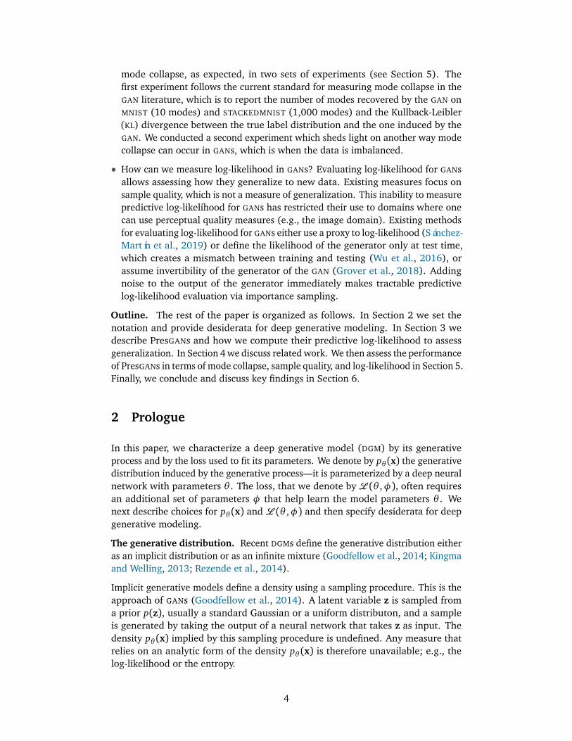
Figure 1: Density estimation with GAN and PresGAN on a toy two-dimensionalexperiment. The ground truth is a uniform mixture of 10 Gaussians organizedon a ring. Given the right set of hyperparameters, a GAN could perfectly fit thistarget distribution. In this example we chose the GAN hyperparameters such that itcollapses—here 4 out of 10 modes are missing. We then fit the PresGAN using thesame hyperparameters as the collapsing GAN. The PresGAN is able to correct thecollapsing behavior of the GAN and learns a good fit for the target distribution.
GANs learn densities by defining a sampling procedure. A latent variable z is sampledfrom a prior p(z) and a sample x(z;θ ) is generated by taking the output of a neuralnetwork with parameters θ , called a generator, that takes z as input. The densitypθ (x) implied by this sampling procedure is implicit and undefined (Mohamedand Lakshminarayanan, 2016). However, GANs effectively learn the parameters θby introducing a classifier Dφ—a deep neural network with parameters φ, calleddiscriminator—that distinguishes between generated samples x(z;θ ) and real datax, with distribution pd(x). The parameters θ and φ are learned jointly by optimizingthe GAN objective,
LGAN(θ ,φ) = Ex∼pd (x)�
log Dφ(x)�
+Ez∼p(z)�
log�
1− Dφ(x(z;θ ))��
. (1)
GANs iteratively maximize the loss in Eq. 1 with respect to φ and minimize it withrespect to θ .
In practice, the minimax procedure described above is stopped when the generatorproduces realistic images. This is problematic because high perceptual quality doesnot necessarily correlate with goodness of fit to the target density. For example,memorizing the training data is a trivial solution to achieving high perceptual quality.Fortunately, GANs do not merely memorize the training data (Zhang et al., 2017;Arora et al., 2017).
However GANs are able to produce images indistinguishable from real images whilestill failing to fully capture the target distribution (Brock et al., 2018; Karras et al.,2019). Indeed GANs suffer from an issue known as mode collapse. When modecollapse happens, the generative distribution pθ (x) is degenerate and of low sup-port (Arora et al., 2017, 2018). Mode collapse causes GANs, as density estimators,to fail both qualitatively and quantitatively. Qualitatively, mode collapse causes lackof diversity in the generated samples. This is problematic for certain applicationsof GANs, e.g. data augmentation. Quantitatively, mode collapse causes poor gen-eralization to new data. This is because when mode collapse happens, there is a
2
(support) mismatch between the learned distribution pθ (x) and the data distribu-tion. Using annealed importance sampling with a kernel density estimate of thelikelihood, Wu et al. (2016) report significantly worse log-likelihood scores for GANswhen compared to variational auto-encoders (VAEs). Similarly poor generalizationperformance was reported by Grover et al. (2018).
A natural way to prevent mode collapse in GANs is to maximize the entropy of thegenerator (Belghazi et al., 2018). Unfortunately the entropy of GANs is unavailable.This is because the existence of the generative density pθ (x) is not guaranteed(Mohamed and Lakshminarayanan, 2016; Arjovsky et al., 2017).
In this paper, we propose a method to alleviate mode collapse in GANs resultingin a new family of GANs called prescribed GANs (PresGANs). PresGANs preventmode collapse by explicitly maximizing the entropy of the generator. This is doneby augmenting the loss in Eq. 1 with the negative entropy of the generator, suchthat minimizing Eq. 1 with respect to θ corresponds to fitting the data while alsomaximizing the entropy of the generative distribution. The existence of the gen-erative density is guaranteed by adding noise to the output of a density network(MacKay, 1995; Diggle and Gratton, 1984). This process defines the generativedistribution pθ (x), not as an implicit distribution as in standard GANs, but as aninfinite mixture of well-defined densities as in continuous VAEs (Kingma and Welling,2013; Rezende et al., 2014). The generative distribution of PresGANs is thereforevery flexible.
Although the entropy of the generative distribution of PresGANs is well-defined,it is intractable. However, fitting a PresGAN to data only involves computing thegradients of the entropy and not the entropy itself. PresGANs use unbiased MonteCarlo estimates of these gradients.
An illustrative example. To demonstrate how PresGANs alleviate mode collapse,we form a target distribution by organizing a uniform mixture of K = 10 two-dimensional Gaussians on a ring. We draw 5,000 samples from this target distribu-tion. We first fit a GAN, setting the hyperparameters so that the GAN suffers frommode collapse2. We then use the same settings for PresGAN to assess whether it cancorrect the collapsing behavior of the GAN. Figure 1 shows the collapsing behaviorof the GAN, which misses 4 modes of the target distribution. The PresGAN, on theother hand, recovers all the modes. Section 5 provides details about the settings ofthis synthetic experiment.
Contributions. This paper contributes to the literature on the two main openproblems in the study of GANs: preventing mode collapse and evaluating log-likelihood.
• How can we perform entropy regularization of the generator of a GAN so as toeffectively prevent mode collapse? We achieve this by adding noise to the outputof the generator; this ensures the existence of a density pθ (x) and makes itsentropy well-defined. We then regularize the GAN loss to encourage densitiespθ (x) with high entropy. During training, we form unbiased estimators of the(intractable) gradients of the entropy regularizer. We show how this prevents
2A GAN can perfectly fit this distribution when choosing the right hyperparameters.
3
mode collapse, as expected, in two sets of experiments (see Section 5). Thefirst experiment follows the current standard for measuring mode collapse in theGAN literature, which is to report the number of modes recovered by the GAN onMNIST (10 modes) and STACKEDMNIST (1,000 modes) and the Kullback-Leibler(KL) divergence between the true label distribution and the one induced by theGAN. We conducted a second experiment which sheds light on another way modecollapse can occur in GANs, which is when the data is imbalanced.
• How can we measure log-likelihood in GANs? Evaluating log-likelihood for GANsallows assessing how they generalize to new data. Existing measures focus onsample quality, which is not a measure of generalization. This inability to measurepredictive log-likelihood for GANs has restricted their use to domains where onecan use perceptual quality measures (e.g., the image domain). Existing methodsfor evaluating log-likelihood for GANs either use a proxy to log-likelihood (Sánchez-Martín et al., 2019) or define the likelihood of the generator only at test time,which creates a mismatch between training and testing (Wu et al., 2016), orassume invertibility of the generator of the GAN (Grover et al., 2018). Addingnoise to the output of the generator immediately makes tractable predictivelog-likelihood evaluation via importance sampling.
Outline. The rest of the paper is organized as follows. In Section 2 we set thenotation and provide desiderata for deep generative modeling. In Section 3 wedescribe PresGANs and how we compute their predictive log-likelihood to assessgeneralization. In Section 4 we discuss related work. We then assess the performanceof PresGANs in terms of mode collapse, sample quality, and log-likelihood in Section 5.Finally, we conclude and discuss key findings in Section 6.
2 Prologue
In this paper, we characterize a deep generative model (DGM) by its generativeprocess and by the loss used to fit its parameters. We denote by pθ (x) the generativedistribution induced by the generative process—it is parameterized by a deep neuralnetwork with parameters θ . The loss, that we denote by L (θ ,φ), often requiresan additional set of parameters φ that help learn the model parameters θ . Wenext describe choices for pθ (x) and L (θ ,φ) and then specify desiderata for deepgenerative modeling.
The generative distribution. Recent DGMs define the generative distribution eitheras an implicit distribution or as an infinite mixture (Goodfellow et al., 2014; Kingmaand Welling, 2013; Rezende et al., 2014).
Implicit generative models define a density using a sampling procedure. This is theapproach of GANs (Goodfellow et al., 2014). A latent variable z is sampled froma prior p(z), usually a standard Gaussian or a uniform distributon, and a sampleis generated by taking the output of a neural network that takes z as input. Thedensity pθ (x) implied by this sampling procedure is undefined. Any measure thatrelies on an analytic form of the density pθ (x) is therefore unavailable; e.g., thelog-likelihood or the entropy.
4
An alternative way to define the generative distribution is by using the approach ofVAEs (Kingma and Welling, 2013; Rezende et al., 2014). They define pθ (x) as aninfinite mixture,
pθ (x) =
∫
pθ (x |z) p(z) dz. (2)
Here the mixing distribution is the prior p(z). The conditional distribution pθ (x |z) isan exponential family distribution, such as a Gaussian or a Bernoulli, parameterizedby a neural network with parameters θ . Although both the prior p(z) and pθ (x |z)are simple tractable distributions, the generative distribution pθ (x) is highly flexiblealbeit intractable. Because pθ (x) in Eq. 2 is well-defined, the log-likelihood and theentropy are also well-defined (although they may be analytically intractable).
The loss function. Fitting the models defined above requires defining a learningprocedure by specifying a loss function. GANs introduce a classifier Dφ, a deepneural network parameterized by φ, to discriminate between samples from the datadistribution pd(x) and the generative distribution pθ (x). The auxiliary parametersφ are learned jointly with the model parameters θ by optimizing the loss in Eq. 1.This training procedure leads to high sample quality but often suffers from modecollapse (Arora et al., 2017, 2018).
An alternative approach to learning θ is via maximum likelihood. This requires awell-defined density pθ (x) such as the one in Eq. 2. Although well-defined, pθ (x) isintractable, making it difficult to learn the parameters θ by maximum likelihood.VAEs instead introduce a recognition network—a neural network with parametersφ that takes data x as input and outputs a distribution over the latent variablesz—and maximize a lower bound on log pθ (x) with respect to both θ and φ,
LVAE(θ ,φ) = Epd (x)Eqφ(z |x)
�
logpθ (x,z)qφ(z |x)
�
= −KL(qφ(z |x)pd(x)||pθ (x,z)). (3)
Here KL(·||·) denotes the KL divergence. Maximizing LVAE(θ ,φ) is equivalent tominimizing this KL which leads to issues such as latent variable collapse (Bowmanet al., 2015; Dieng et al., 2018b). Furthermore, optimizing Eq. 3 may lead toblurriness in the generated samples because of a property of the reverse KL knownas zero-forcing (Minka et al., 2005).
Desiderata. We now outline three desiderata for DGMs.
High sample quality. A DGM whose parameters θ have been fitted using real datashould generate new data with the same qualitative precision as the data it wastrained with. For example, if a DGM is trained on a dataset composed of humanfaces, it should generate data with all features that make up a face at the sameresolution as the training data.
High sample diversity. High sample quality alone is not enough. For example, adegenerate DGM that is only able to produce one single sample is not desirable,even if the sample quality is perfect. Therefore we require sample diversity; a DGM
should ideally capture all modes of the data distribution.
Tractable predictive log-likelihood. DGMs are density estimators and as such we shouldevaluate how they generalize to new data. High sample quality and diversity are not
5
measures of generalization. We therefore require tractable predictive log-likelihoodas a desideratum for deep generative modeling.
We next introduce a new family of GANs that fulfills all the desiderata.
3 Prescribed Generative Adversarial Networks
PresGANs generate data following the generative distribution in Eq. 2. Note thatthis generative process is the same as for standard VAEs (Kingma and Welling, 2013;Rezende et al., 2014). In particular, PresGANs set the prior p(z) and the likelihoodpθ (x |z) to be Gaussians,
p(z) =N (z |0, I) and pθ (x |z) =N (x |µθ (z),Σθ (z)) . (4)
The mean µθ (z) and covariance Σθ (z) of the conditional pθ (x |z) are given by aneural network that takes z as input.
In general, both the mean µθ (z) and the covariance Σθ (z) can be functions of z.For simplicity, in order to speed up the learning procedure, we set the covariancematrix to be diagonal with elements independent from z, i.e., Σθ (z) = diag
�
σ2�
,and we learn the vector σ together with θ . From now on, we parameterize themean with η, write µη(z), and define θ = (η,σ) as the parameters of the generativedistribution.
To fit the model parameters θ , PresGANs optimize an adversarial loss similarly toGANs. In doing so, they keep GANs’ ability to generate samples with high perceptualquality. Unlike GANs, the entropy of the generative distribution of PresGANs iswell-defined, and therefore PresGANs can prevent mode collapse by adding anentropy regularizer to Eq. 1. Furthermore, because PresGANs define a density overtheir generated samples, we can measure how they generalize to new data usingpredictive log-likelihood. We describe the entropy regularization in Section 3.1 andhow to approximate the predictive log-likelihood in Section 3.3.
3.1 Avoiding mode collapse via entropy regularization
One of the major issues that GANs face is mode collapse, where the generator tendsto model only some parts or modes of the data distribution (Arora et al., 2017,2018). PresGANs mitigate this problem by explicitly maximizing the entropy of thegenerative distribution,
LPresGAN(θ ,φ) =LGAN(θ ,φ)−λH (pθ (x)) . (5)
HereH (pθ (x)) denotes the entropy of the generative distribution. It is defined as
H (pθ (x)) = −Epθ (x) [log pθ (x)] . (6)
The loss LGAN(θ ,φ) in Eq. 5 can be that of any of the existing GAN variants. InSection 5 we explore the standard deep convolutional generative adversarial network
6
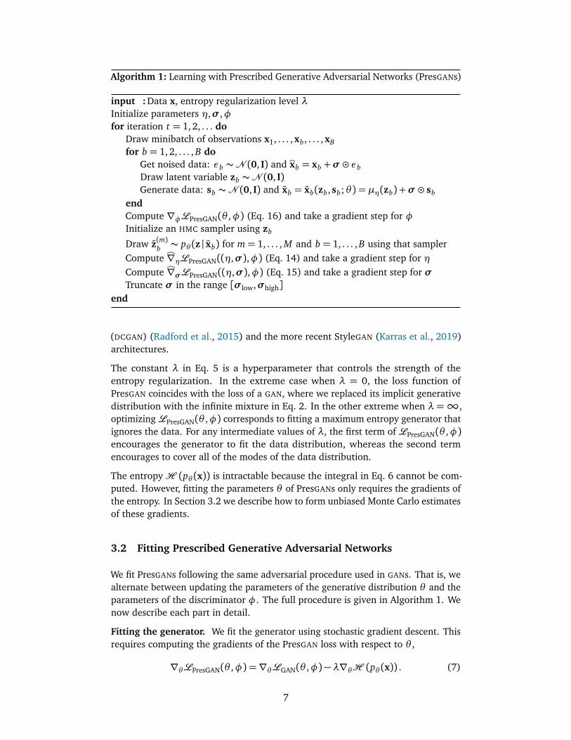
Algorithm 1: Learning with Prescribed Generative Adversarial Networks (PresGANs)
input : Data x, entropy regularization level λInitialize parameters η,σ,φfor iteration t = 1, 2, . . . do
Draw minibatch of observations x1, . . . ,xb, . . . ,xBfor b = 1, 2, . . . , B do
endCompute ∇φLPresGAN(θ ,φ) (Eq. 16) and take a gradient step for φInitialize an HMC sampler using zb
Draw z(m)b ∼ pθ (z | xb) for m= 1, . . . , M and b = 1, . . . , B using that samplerCompute Ò∇ηLPresGAN((η,σ),φ) (Eq. 14) and take a gradient step for ηCompute Ò∇σLPresGAN((η,σ),φ) (Eq. 15) and take a gradient step for σTruncate σ in the range [σlow,σhigh]
end
(DCGAN) (Radford et al., 2015) and the more recent StyleGAN (Karras et al., 2019)architectures.
The constant λ in Eq. 5 is a hyperparameter that controls the strength of theentropy regularization. In the extreme case when λ = 0, the loss function ofPresGAN coincides with the loss of a GAN, where we replaced its implicit generativedistribution with the infinite mixture in Eq. 2. In the other extreme when λ=∞,optimizingLPresGAN(θ ,φ) corresponds to fitting a maximum entropy generator thatignores the data. For any intermediate values of λ, the first term of LPresGAN(θ ,φ)encourages the generator to fit the data distribution, whereas the second termencourages to cover all of the modes of the data distribution.
The entropyH (pθ (x)) is intractable because the integral in Eq. 6 cannot be com-puted. However, fitting the parameters θ of PresGANs only requires the gradients ofthe entropy. In Section 3.2 we describe how to form unbiased Monte Carlo estimatesof these gradients.
We fit PresGANs following the same adversarial procedure used in GANs. That is, wealternate between updating the parameters of the generative distribution θ and theparameters of the discriminator φ. The full procedure is given in Algorithm 1. Wenow describe each part in detail.
Fitting the generator. We fit the generator using stochastic gradient descent. Thisrequires computing the gradients of the PresGAN loss with respect to θ ,
We form stochastic estimates of∇θLGAN(θ ,φ) based on reparameterization (Kingmaand Welling, 2013; Rezende et al., 2014; Titsias and Lázaro-Gredilla, 2014); thisrequires differentiating Eq. 1. Specifically, we introduce a noise variable ε to repa-rameterize the conditional from Eq. 4,3
x(z,ε;θ ) = µη(z) +σ � ε, (8)
where θ = (η,σ) and ε∼N (0, I). Here µη(z) andσ denote the mean and standarddeviation of the conditional pθ (x |z), respectively. We now write the first term ofEq. 7 as an expectation with respect to the latent variable z and the noise variable εand push the gradient into the expectation,
∇θLGAN(θ ,φ) = Ep(z)p(ε)�
∇θ log�
1− Dφ(x(z,ε;θ ))��
. (9)
In practice we use an estimate of Eq. 9 using one sample from p(z) and one samplefrom p(ε),
Ò∇θLGAN(θ ,φ) =∇θ log�
1− Dφ(x(z,ε;θ ))�
. (10)
The second term in Eq. 7, corresponding to the gradient of the entropy, is intractable.We estimate it using the same approach as Titsias and Ruiz (2018). We first use thereparameterization in Eq. 8 to express the gradient of the entropy as an expecta-tion,
where we have used the score function identity Epθ (x) [∇θ log pθ (x)] = 0 on thesecond line. We form a one-sample estimator of the gradient of the entropy as
Ò∇θH (pθ (x)) = −∇xlog pθ (x)�
�
x=x(z,ε;θ ) ×∇θx(z,ε;θ ). (11)
In Eq. 11, the gradient with respect to the reparameterization transformation∇θx(z,ε;θ ) is tractable and can be obtained via back-propagation. We now derive∇x log pθ (x),
∇x log pθ (x) =∇xpθ (x)
pθ (x)=
∫
∇xpθ (x,z)dz
pθ (x)=
∫ ∇xpθ (x |z)pθ (x |z)
pθ (x,z)
pθ (x)dz
=
∫
∇x log pθ (x |z)pθ (z |x)dz= Epθ (z |x) [∇x log pθ (x |z)] .
While this expression is still intractable, we can estimate it. One way is to use self-normalized importance sampling with a proposal learned using moment matching
3With this reparameterization we use the notation x(z,ε;θ ) instead of x(z;θ ) to denote a samplefrom the generative distribution.
8
with an encoder (Dieng and Paisley, 2019). However, this would lead to a biased (al-beit asymptotically unbiased) estimate of the entropy. In this paper, we form an unbi-ased estimate of ∇x log pθ (x) using samples z(1), . . . ,z(M) from the posterior,
Ò∇x log pθ (x) =1M
M∑
m=1
∇x log pθ (x |z(m)), z(m) ∼ pθ (z |x). (12)
We obtain these samples using Hamiltonian Monte Carlo (HMC) (Neal et al., 2011).Crucially, in order to speed up the algorithm, we initialize the HMC sampler atstationarity. That is, we initialize the HMC sampler with the sample z that was usedto produce the generated sample x(z,ε;θ) in Eq. 8, which by construction is anexact sample from pθ (z |x). This implies that only a few HMC iterations suffice toget good estimates of the gradient (Titsias and Ruiz, 2018). We also found thisholds empirically; for example in Section 5 we use 2 burn-in iterations and M = 2HMC samples to form the Monte Carlo estimate in Eq. 12.
Finally, using Eqs. 7 and 10 to 12 we can approximate the gradient of the entropy-regularized adversarial loss with respect to the model parameters θ ,
Ò∇θLPresGAN(θ ,φ) =∇θ log�
1− Dφ(x(z,ε;θ ))�
+λ
M
M∑
m=1
∇x log pθ (x |z(m))�
�
x=x(z(m),ε;θ ) ×∇θx�
z(m),ε;θ�
. (13)
In particular, the gradient with respect to the generator’s parameters η is unbiasedlyapproximated by
Ò∇ηLPresGAN(θ ,φ) =∇η log�
1− Dφ(x(z,ε;θ ))�
−λ
M
M∑
m=1
x(z(m),ε;θ )−µη�
z(m)�
σ2∇ηµη(z(m)), (14)
and the gradient estimator with respect to the standard deviation σ is
Ò∇σLPresGAN(θ ,φ) =∇σ log�
1− Dφ(x(z,ε;θ ))�
−λ
M
M∑
m=1
x(z(m),ε;θ )−µη�
z(m)�
σ2· ε. (15)
These gradients are used in a stochastic optimization algorithm to fit the generativedistribution of PresGAN.
Fitting the discriminator. Since the entropy term in Eq. 5 does not dependon φ, optimizing the discriminator of a PresGAN is analogous to optimizing thediscriminator of a GAN,
∇φLPresGAN(θ ,φ) =∇φLGAN(θ ,φ). (16)
To prevent the discriminator from getting stuck in a bad local optimum where itcan perfectly distinguish between real and generated data by relying on the addednoise, we apply the same amount of noise to the real data x as the noise added to
9
the generated data. That is, when we train the discriminator we corrupt the realdata according to
bx= x+σ � ε, (17)
where σ is the standard deviation of the generative distribution and x denotes thereal data. We then let the discriminator distinguish between bx and x(z,ε;θ) fromEq. 8.
This data noising procedure is a form of instance noise (Sønderby et al., 2016).However, instead of using a fixed annealing schedule for the noise variance asSønderby et al. (2016), we let σ be part of the parameters of the generativedistribution and fit it using gradient descent according to Eq. 15.
Stability. Data noising stabilizes the training procedure and prevents the discrimi-nator from perfectly being able to distinguish between real and generated samplesusing the background noise. We refer the reader to Huszár (2016) for a detailedexposition.
When fitting PresGANs, data noising is not enough to stabilize training. This isbecause there are two failure cases brought in by learning the variance σ2 usinggradient descent. The first failure mode is when the variance gets very large, leadingto a generator completely able to fool the discriminator. Because of data noising,the discriminator cannot distinguish between real and generated samples when thevariance of the noise is large.
The second failure mode is when σ2 gets very small, which makes the gradientof the entropy in Eq. 14 dominate the overall gradient of the generator. This isproblematic because the learning signal from the discriminator is lost.
To stabilize training and avoid the two failure cases discussed above we truncate thevariance of the generative distribution, σlow ≤ σ ≤ σhigh (we apply this truncationelement-wise). The limits σlow and σhigh are hyperparameters.
Replacing the implicit generative distribution of GANs with the infinite mixturedistribution defined in Eq. 2 has the advantage that the predictive log-likelihoodcan be tractably approximated. Consider an unseen datapoint x∗. We estimate itslog marginal likelihood log pθ (x∗) using importance sampling,
log pθ (x∗)≈ log
�
1S
S∑
s=1
pθ�
x∗ |z(s)�
· p�
z(s)�
r�
z(s) |x∗�
�
, (18)
where we draw S samples z(1), . . . ,z(S) from a proposal distribution r(z |x∗).
There are different ways to form a good proposal r(z |x∗), and we discuss severalalternatives in Section 7.1 of the appendix. In this paper, we take the followingapproach. We define the proposal as a Gaussian distribution,
r(z |x∗) =N (µr ,Σr). (19)
10
We set the mean parameter µr to the maximum a posteriori solution, i.e., µr =argmaxz (log pθ (x∗ |z) + log p (z)). We initialize this maximization algorithm usingthe mean of a pre-fitted encoder, qγ(z |x∗). The encoder is fitted by minimizing thereverse KL divergence between qγ(z |x) and the true posterior pθ (z |x) using thetraining data. This KL is
KL�
qγ(z |x)||pθ (z |x)�
= log pθ (x)−Eqγ(z |x)�
log pθ (x |z)p(z)− log qγ(z |x)�
.
(20)
Because the generative distribution is fixed at test time, minimizing the KL here isequivalent to maximizing the second term in Eq. 20, which is the evidence lowerbound (ELBO) objective of VAEs.
We set the proposal covariance Σr as an overdispersed version4 of the encoder’scovariance matrix, which is diagonal. In particular, to obtain Σr we multiplythe elements of the encoder’s covariance by a factor γ. In Section 5 we set γto 1.2.
4 Related Work
GANs (Goodfellow et al., 2014) have been extended in multiple ways, using alterna-tive distance metrics and optimization methods (see, e.g., Li et al., 2015; Dziugaiteet al., 2015; Nowozin et al., 2016; Arjovsky et al., 2017; Ravuri et al., 2018; Genevayet al., 2017) or using ideas from VAEs (Makhzani et al., 2015; Mescheder et al.,2017; Dumoulin et al., 2016; Donahue et al., 2016; Tolstikhin et al., 2017; Ulyanovet al., 2018; Rosca et al., 2017).
Other extensions aim at improving the sample diversity of GANs. For example,Srivastava et al. (2017) use a reconstructor network that reverses the action of thegenerator. Lin et al. (2018) use multiple observations (either real or generated) asan input to the discriminator to prevent mode collapse. Azadi et al. (2018) andTurner et al. (2018) use sampling mechanisms to correct errors of the generativedistribution. Xiao et al. (2018) relies on identifying the geometric structure ofthe data embodied under a specific distance metric. Other works have combinedadversarial learning with maximum likelihood (Grover et al., 2018; Yin and Zhou,2019); however, the low sample quality induced by maximum likelihood still occurs.Finally, Cao et al. (2018) introduce a regularizer for the discriminator to encouragediverse activation patterns in the discriminator across different samples. In contrastto these works, PresGANs regularize the entropy of the generator to prevent modecollapse.
The idea of entropy regularization has been widely applied in many problemsthat involve estimation of unknown probability distributions. Examples includeapproximate Bayesian inference, where the variational objective contains an entropypenalty (Jordan, 1998; Bishop, 2006; Wainwright et al., 2008; Blei et al., 2017);reinforcement learning, where the entropy regularization allows to estimate moreuncertain and explorative policies (Schulman et al., 2015; Mnih et al., 2016);
4In general, overdispersed proposals lead to better importance sampling estimates.
11
statistical learning, where entropy regularization allows an inferred probabilitydistribution to avoid collapsing to a deterministic solution (Freund and Schapire,1997; Soofi, 2000; Jaynes, 2003); or optimal transport (Rigollet and Weed, 2018).More recently, Kumar et al. (2019) have developed maximum-entropy generatorsfor energy-based models using mutual information as a proxy for entropy.
Another body of related work is about how to quantitatively evaluate GANs. Inceptionscores measure the sample quality of GANs and are used extensively in the GAN
literature (Salimans et al., 2016; Heusel et al., 2017; Binkowski et al., 2018).However, sample quality measures only assess the quality of GANs as data generatorsand not as density estimators. Density estimators are evaluated for generalizationto new data. Predictive log-likelihood is a measure of goodness of fit that hasbeen used to assess generalization; for example in VAEs. Finding ways to evaluatepredictive log-likelihood for GANs has been an open problem, because GANs do notdefine a density on the generated samples. Wu et al. (2016) use a kernel densityestimate (Parzen, 1962) and estimate the log-likelihood with annealed importancesampling (Neal, 2001). Balaji et al. (2018) show that an optimal transport GAN
with entropy regularization can be viewed as a generative model that maximizes avariational lower bound on average sample likelihoods, which relates to the approachof VAEs (Kingma and Welling, 2013). Sánchez-Martín et al. (2019) propose EvalGAN,a method to estimate the likelihood. Given an observation x?, EvalGAN first findsthe closest observation ex that the GAN is able to generate, and then it estimatesthe likelihood p(x?) by approximating the proportion of samples z ∼ p(z) thatlead to samples x that are close to ex. EvalGAN requires selecting an appropriatedistance metric for each problem and evaluates GANs trained with the usual implicitgenerative distribution. Finally, Grover et al. (2018) assume invertibility of thegenerator to make log-likelihood tractable.
5 Empirical Study
Here we demonstrate PresGANs’ ability to prevent mode collapse and generatehigh-quality samples. We also evaluate its predictive performance as measured bylog-likelihood.
5.1 An Illustrative Example
In this section, we fit a GAN to a toy synthetic dataset of 10 modes. We choose thehyperparameters such that the GAN collapses. We then apply these same hyperparam-eters to fit a PresGAN on the same synthetic dataset. This experiment demonstratesthe PresGAN’s ability to correct the mode collapse problem of a GAN.
We form the target distribution by organizing a uniform mixture of K = 10 two-dimensional Gaussians on a ring. The radius of the ring is r = 3 and each Gaussianhas standard deviation 0.05. We then slice the circle into K parts. The location ofthe centers of the mixture components are determined as follows. Consider the kth
12
mixture component. Its coordinates in the 2D space are
centerx = r · cos�
k ·2πK
�
and centery = r · sin�
k ·2πK
�
.
We draw 5,000 samples from the target distribution and fit a GAN and a PresGAN.
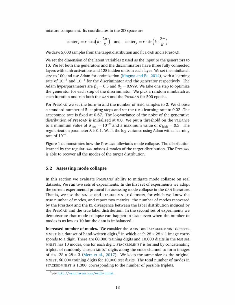
We set the dimension of the latent variables z used as the input to the generators to10. We let both the generators and the discriminators have three fully connectedlayers with tanh activations and 128 hidden units in each layer. We set the minibatchsize to 100 and use Adam for optimization (Kingma and Ba, 2014), with a learningrate of 10−3 and 10−4 for the discriminator and the generator respectively. TheAdam hyperparameters are β1 = 0.5 and β2 = 0.999. We take one step to optimizethe generator for each step of the discriminator. We pick a random minibatch ateach iteration and run both the GAN and the PresGAN for 500 epochs.
For PresGAN we set the burn-in and the number of HMC samples to 2. We choosea standard number of 5 leapfrog steps and set the HMC learning rate to 0.02. Theacceptance rate is fixed at 0.67. The log-variance of the noise of the generativedistribution of PresGAN is initialized at 0.0. We put a threshold on the varianceto a minimum value of σlow = 10−2 and a maximum value of σhigh = 0.3. Theregularization parameter λ is 0.1. We fit the log-variance using Adam with a learningrate of 10−4.
Figure 1 demonstrates how the PresGAN alleviates mode collapse. The distributionlearned by the regular GAN misses 4 modes of the target distribution. The PresGAN
is able to recover all the modes of the target distribution.
5.2 Assessing mode collapse
In this section we evaluate PresGANs’ ability to mitigate mode collapse on realdatasets. We run two sets of experiments. In the first set of experiments we adoptthe current experimental protocol for assessing mode collapse in the GAN literature.That is, we use the MNIST and STACKEDMNIST datasets, for which we know thetrue number of modes, and report two metrics: the number of modes recoveredby the PresGAN and the KL divergence between the label distribution induced bythe PresGAN and the true label distribution. In the second set of experiments wedemonstrate that mode collapse can happen in GANs even when the number ofmodes is as low as 10 but the data is imbalanced.
Increased number of modes. We consider the MNIST and STACKEDMNIST datasets.MNIST is a dataset of hand-written digits,5 in which each 28× 28× 1 image corre-sponds to a digit. There are 60,000 training digits and 10,000 digits in the test set.MNIST has 10 modes, one for each digit. STACKEDMNIST is formed by concatenatingtriplets of randomly chosen MNIST digits along the color channel to form imagesof size 28 × 28 × 3 (Metz et al., 2017). We keep the same size as the originalMNIST, 60,000 training digits for 10,000 test digits. The total number of modes inSTACKEDMNIST is 1,000, corresponding to the number of possible triplets.
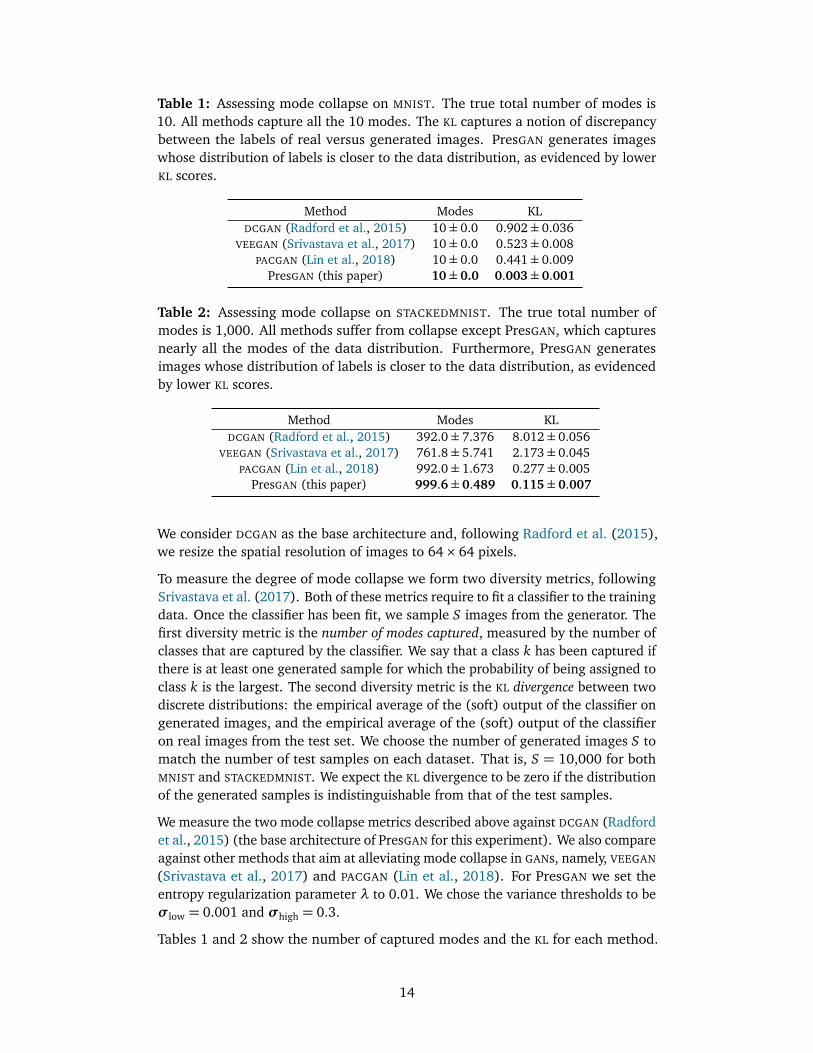
Table 1: Assessing mode collapse on MNIST. The true total number of modes is10. All methods capture all the 10 modes. The KL captures a notion of discrepancybetween the labels of real versus generated images. PresGAN generates imageswhose distribution of labels is closer to the data distribution, as evidenced by lowerKL scores.
VEEGAN (Srivastava et al., 2017) 10± 0.0 0.523± 0.008PACGAN (Lin et al., 2018) 10± 0.0 0.441± 0.009
PresGAN (this paper) 10± 0.0 0.003± 0.001
Table 2: Assessing mode collapse on STACKEDMNIST. The true total number ofmodes is 1,000. All methods suffer from collapse except PresGAN, which capturesnearly all the modes of the data distribution. Furthermore, PresGAN generatesimages whose distribution of labels is closer to the data distribution, as evidencedby lower KL scores.
VEEGAN (Srivastava et al., 2017) 761.8± 5.741 2.173± 0.045PACGAN (Lin et al., 2018) 992.0± 1.673 0.277± 0.005
PresGAN (this paper) 999.6± 0.489 0.115± 0.007
We consider DCGAN as the base architecture and, following Radford et al. (2015),we resize the spatial resolution of images to 64× 64 pixels.
To measure the degree of mode collapse we form two diversity metrics, followingSrivastava et al. (2017). Both of these metrics require to fit a classifier to the trainingdata. Once the classifier has been fit, we sample S images from the generator. Thefirst diversity metric is the number of modes captured, measured by the number ofclasses that are captured by the classifier. We say that a class k has been captured ifthere is at least one generated sample for which the probability of being assigned toclass k is the largest. The second diversity metric is the KL divergence between twodiscrete distributions: the empirical average of the (soft) output of the classifier ongenerated images, and the empirical average of the (soft) output of the classifieron real images from the test set. We choose the number of generated images S tomatch the number of test samples on each dataset. That is, S = 10,000 for bothMNIST and STACKEDMNIST. We expect the KL divergence to be zero if the distributionof the generated samples is indistinguishable from that of the test samples.
We measure the two mode collapse metrics described above against DCGAN (Radfordet al., 2015) (the base architecture of PresGAN for this experiment). We also compareagainst other methods that aim at alleviating mode collapse in GANs, namely, VEEGAN
(Srivastava et al., 2017) and PACGAN (Lin et al., 2018). For PresGAN we set theentropy regularization parameter λ to 0.01. We chose the variance thresholds to beσlow = 0.001 and σhigh = 0.3.
Tables 1 and 2 show the number of captured modes and the KL for each method.
14
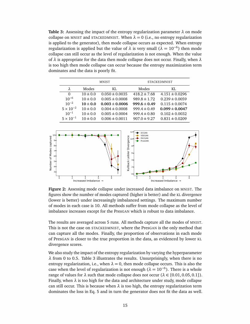
Table 3: Assessing the impact of the entropy regularization parameter λ on modecollapse on MNIST and STACKEDMNIST. When λ= 0 (i.e., no entropy regularizationis applied to the generator), then mode collapse occurs as expected. When entropyregularization is applied but the value of λ is very small (λ = 10−6) then modecollapse can still occur as the level of regularization is not enough. When the valueof λ is appropriate for the data then mode collapse does not occur. Finally, when λis too high then mode collapse can occur because the entropy maximization termdominates and the data is poorly fit.
Figure 2: Assessing mode collapse under increased data imbalance on MNIST. Thefigures show the number of modes captured (higher is better) and the KL divergence(lower is better) under increasingly imbalanced settings. The maximum numberof modes in each case is 10. All methods suffer from mode collapse as the level ofimbalance increases except for the PresGAN which is robust to data imbalance.
The results are averaged across 5 runs. All methods capture all the modes of MNIST.This is not the case on STACKEDMNIST, where the PresGAN is the only method thatcan capture all the modes. Finally, the proportion of observations in each modeof PresGAN is closer to the true proportion in the data, as evidenced by lower KL
divergence scores.
We also study the impact of the entropy regularization by varying the hyperparameterλ from 0 to 0.5. Table 3 illustrates the results. Unsurprisingly, when there is noentropy regularization, i.e., when λ = 0, then mode collapse occurs. This is also thecase when the level of regularization is not enough (λ= 10−6). There is a wholerange of values for λ such that mode collapse does not occur (λ ∈ {0.01, 0.05, 0.1}).Finally, when λ is too high for the data and architecture under study, mode collapsecan still occur. This is because when λ is too high, the entropy regularization termdominates the loss in Eq. 5 and in turn the generator does not fit the data as well.
15
This is also evidenced by the higher KL divergence score when λ = 0.5 vs. when0< λ < 0.5.
Increased data imbalance. We now show that mode collapse can occur in GANswhen the data is imbalanced, even when the number of modes of the data distri-bution is small. We follow Dieng et al. (2018a) and consider a perfectly balancedversion of MNIST as well as nine imbalanced versions. To construct the balanceddataset we used 5,000 training examples per class, totaling 50,000 training exam-ples. We refer to this original balanced dataset as D0. Each additional training setDk leaves only 5 training examples for each class j ≤ k, and 5,000 for the rest. (Seethe Appendix for all the class distributions.)
We used the same classifier trained on the unmodified MNIST but fit each methodon each of the 9 new MNIST distributions. We chose λ= 0.1 for PresGAN. Figure 2illustrates the results in terms of both metrics—number of modes and KL divergence.DCGAN, VEEGAN, and PACGAN face mode collapse as the level of imbalance increases.This is not the case for PresGAN, which is robust to imbalance and captures all the10 modes.
5.3 Assessing sample quality
In this section we assess PresGANs’ ability to generate samples of high perceptualquality. We rely on perceptual quality of generated samples and on Fréchet Inceptiondistance (FID) scores (Heusel et al., 2017). We also consider two different GAN
architectures, the standard DCGAN and the more recent StyleGAN, to show robustnessof PresGANs vis-a-vis the underlying GAN architecture.
DCGAN. We use DCGAN (Radford et al., 2015) as the base architecture and buildPresGAN on top of it. We consider four datasets: MNIST, STACKEDMNIST, CIFAR-10, and CelebA. CIFAR-10 (Krizhevsky et al., 2009) is a well-studied dataset of32× 32 images that are classified into one of the following categories: airplane,automobile, bird, cat, deer, dog, frog, horse, ship, and truck. CelebA (Liu et al.,2015) is a large-scale face attributes dataset. Following Radford et al. (2015),we resize all images to 64 × 64 pixels. We use the default DCGAN settings. Werefer the reader to the code we used for DCGAN, which was taken from https://github.com/pytorch/examples/tree/master/dcgan. We set the seed to 2019for reproducibility.
There are hyperparameters specific to PresGAN. These are the noise and HMC
hyperparameters. We set the learning rate for the noise parameters σ to 10−3 andconstrain its values to be between 10−3 and 0.3 for all datasets. We initialize logσto −0.5. We set the burn-in and the number of HMC samples to 2. We choose astandard number of 5 leapfrog steps and set the HMC learning rate to 0.02. Theacceptance rate is fixed at 0.67. We found that different λ values worked betterfor different datasets. We used λ= 5× 10⁻⁴ for CIFAR-10 and CELEBA λ= 0.01 forMNIST and STACKEDMNIST.
We found the PresGAN’s performance to be robust to the default settings for most ofthese hyperparameters. However we found the initialization for σ and its learning
rate to play a role in the quality of the generated samples. The hyperparametersmentioned above for σ worked well for all datasets.
Table 4 shows the FID scores for DCGAN and PresGAN across the four datasets. Wecan conclude that PresGAN generates images of high visual quality. In addition, theFID scores are lower because PresGAN explores more modes than DCGAN. Indeed,when the generated images account for more modes, the FID sufficient statistics(the mean and covariance of the Inception-v3 pool3 layer) of the generated dataget closer to the sufficient statistics of the empirical data distribution.
We also report the FID for VEEGAN and PACGAN in Table 4. VEEGAN achieves betterFID scores than DCGAN on all datasets but CELEBA. This is because VEEGAN collapsesless than DCGAN as evidenced by Table 1 and Table 2. PACGAN achieves better FID
scores than both DCGAN and VEEGAN on all datasets but on STACKEDMNIST where itachieves a significantly worse FID score. Finally, PresGAN outperforms all of thesemethods on the FID metric on all datasets signaling its ability to mitigate modecollapse while preserving sample quality.
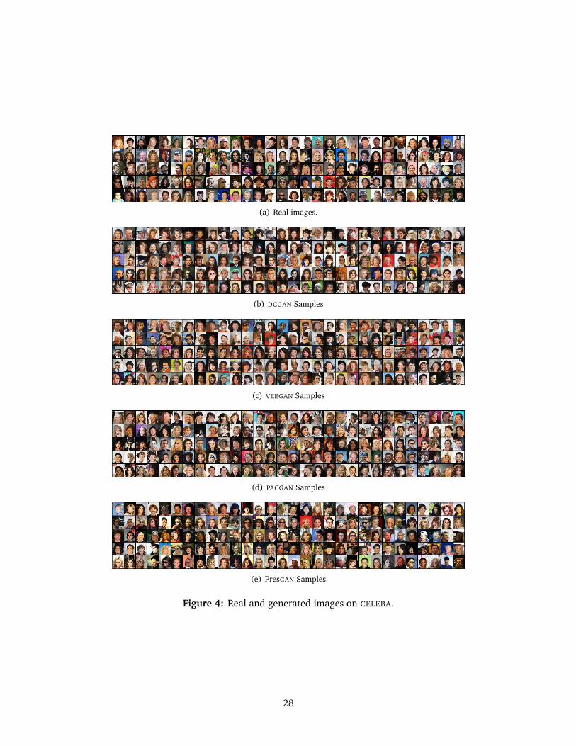
Besides the FID scores, we also assess the visual quality of the generated images.In Section 7.3 of the appendix, we show randomly generated (not cherry-picked)images from DCGAN, VEEGAN, PACGAN, and PresGAN. For PresGAN, we show themean of the conditional distribution of x given z. The samples generated by PresGAN
have high visual quality; in fact their quality is comparable to or better than theDCGAN samples.
StyleGAN. We now consider a more recent GAN architecture (StyleGAN) (Karraset al., 2019) and a higher resolution image dataset (FFHQ). FFHQ is a diverse dataset
17
Figure 3: Generated images on FFHQ for StyleGAN (left) and PresGAN (right). ThePresGAN maintains the high perceptual quality of the StyleGAN.
of faces from Flickr6 introduced by Karras et al. (2019). The dataset contains 70,000high-quality PNG images with considerable variation in terms of age, ethnicity, andimage background. We use a resolution of 128× 128 pixels.
StyleGAN feeds multiple sources of noise z to the generator. In particular, it addsGaussian noise after each convolutional layer before evaluating the nonlinearity.Building PresGAN on top of StyleGAN therefore requires to sample all noise variablesz through HMC at each training step. To speed up the training procedure, we onlysample the noise variables corresponding to the input latent code and condition onall the other Gaussian noise variables. In addition, we do not follow the progressivegrowing of the networks of Karras et al. (2019) for simplicity.
For this experiment, we choose the same HMC hyperparameters as for the previousexperiments but restrict the variance of the generative distribution to be σhigh = 0.2.We set λ= 0.001 for this experiment.
Figure 3 shows cherry-picked images generated from StyleGAN and PresGAN. Wecan observe that the PresGAN maintains as good perceptual quality as the basearchitecture. In addition, we also observed that the StyleGAN tends to produce
some redundant images (these are not shown in Figure 3), something that we didnot observe with the PresGAN. This lack of diversity was also reflected in the FID
scores which were 14.72± 0.09 for StyleGAN and 12.15± 0.09 for PresGAN. Theseresults suggest that entropy regularization effectively reduces mode collapse whilepreserving sample quality.
5.4 Assessing held-out predictive log-likelihood
In this section we evaluate PresGANs for generalization using predictive log-likelihood.We use the DCGAN architecture to build PresGAN and evaluate the log-likelihood ontwo benchmark datasets, MNIST and CIFAR-10. We use images of size 32×32.
We compare the generalization performance of the PresGAN against the VAE (Kingmaand Welling, 2013; Rezende et al., 2014) by controlling for the architecture andthe evaluation procedure. In particular, we fit a VAE that has the same decoderarchitecture as the PresGAN. We form the VAE encoder by using the same architectureas the DCGAN discriminator and getting rid of the output layer. We used linear mapsto get the mean and the log-variance of the approximate posterior.
To measure how PresGANs compare to traditional GANs in terms of log-likelihood,we also fit a PresGAN with λ= 0.
Evaluation. We control for the evaluation procedure and follow what’s describedin Section 3.3 for all methods. We use S = 2,000 samples to form the importancesampling estimator. Since the pixel values are normalized in [−1,+1], we use atruncated Gaussian likelihood for evaluation. Specifically, for each pixel of the testimage, we divide the Gaussian likelihood by the probability (under the generativemodel) that the pixel is within the interval [−1,+1]. We use the truncated Gaussianlikelihood at test time only.
Settings. For the PresGAN, we use the same HMC hyperparameters as for theprevious experiments. We constrain the variance of the generative distribution usingσlow = 0.001 and σhigh = 0.2. We use the default DCGAN values for the remaininghyperparameters, including the optimization settings. For the CIFAR-10 experiment,we choose λ= 0.001. We set all learning rates to 0.0002. We set the dimension ofthe latent variables to 100. We ran both the VAE and the PresGAN for a maximum of200 epochs. For MNIST, we use the same settings as for CIFAR-10 but use λ = 0.0001and ran all methods for a maximum of 50 epochs.
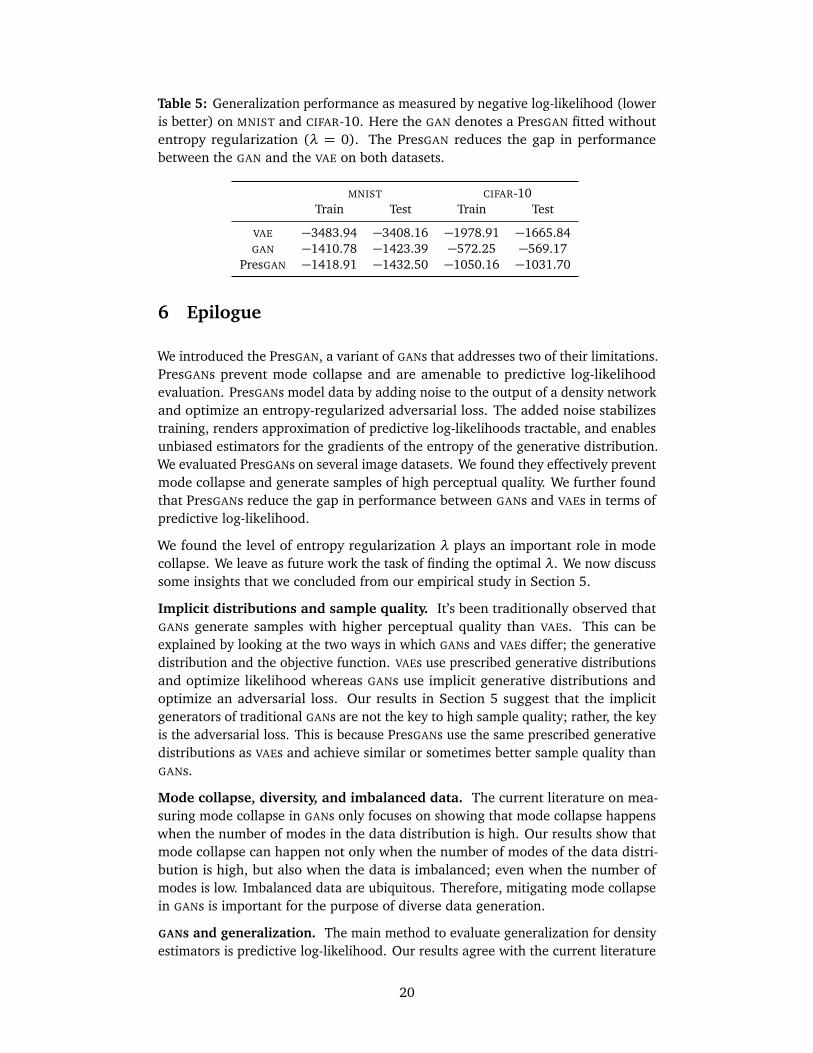
Results. Table 5 summarizes the results. Here GAN denotes the PresGAN fittedusing λ = 0. The VAE outperforms both the GAN and the PresGAN on both MNIST
and CIFAR-10. This is unsurprising given VAEs are fitted to maximize log-likelihood.The GAN’s performance on CIFAR-10 is particularly bad, suggesting it suffered frommode collapse. The PresGAN, which mitigates mode collapse achieves significantlybetter performance than the GAN on CIFAR-10. To further analyze the generalizationperformance, we also report the log-likelihood on the training set in Table 5. Wecan observe that the difference between the training log-likelihood and the testlog-likelihood is very small for all methods.
19
Table 5: Generalization performance as measured by negative log-likelihood (loweris better) on MNIST and CIFAR-10. Here the GAN denotes a PresGAN fitted withoutentropy regularization (λ = 0). The PresGAN reduces the gap in performancebetween the GAN and the VAE on both datasets.
We introduced the PresGAN, a variant of GANs that addresses two of their limitations.PresGANs prevent mode collapse and are amenable to predictive log-likelihoodevaluation. PresGANs model data by adding noise to the output of a density networkand optimize an entropy-regularized adversarial loss. The added noise stabilizestraining, renders approximation of predictive log-likelihoods tractable, and enablesunbiased estimators for the gradients of the entropy of the generative distribution.We evaluated PresGANs on several image datasets. We found they effectively preventmode collapse and generate samples of high perceptual quality. We further foundthat PresGANs reduce the gap in performance between GANs and VAEs in terms ofpredictive log-likelihood.
We found the level of entropy regularization λ plays an important role in modecollapse. We leave as future work the task of finding the optimal λ. We now discusssome insights that we concluded from our empirical study in Section 5.
Implicit distributions and sample quality. It’s been traditionally observed thatGANs generate samples with higher perceptual quality than VAEs. This can beexplained by looking at the two ways in which GANs and VAEs differ; the generativedistribution and the objective function. VAEs use prescribed generative distributionsand optimize likelihood whereas GANs use implicit generative distributions andoptimize an adversarial loss. Our results in Section 5 suggest that the implicitgenerators of traditional GANs are not the key to high sample quality; rather, the keyis the adversarial loss. This is because PresGANs use the same prescribed generativedistributions as VAEs and achieve similar or sometimes better sample quality thanGANs.
Mode collapse, diversity, and imbalanced data. The current literature on mea-suring mode collapse in GANs only focuses on showing that mode collapse happenswhen the number of modes in the data distribution is high. Our results show thatmode collapse can happen not only when the number of modes of the data distri-bution is high, but also when the data is imbalanced; even when the number ofmodes is low. Imbalanced data are ubiquitous. Therefore, mitigating mode collapsein GANs is important for the purpose of diverse data generation.
GANs and generalization. The main method to evaluate generalization for densityestimators is predictive log-likelihood. Our results agree with the current literature
20
that GANs don’t generalize as well as VAEs which are specifically trained to maximizelog-likelihood. However, our results show that entropy-regularized adversariallearning can reduce the gap in generalization performance between GANs andVAEs. Methods that regularize GANs with the maximum likelihood objective achievegood generalization performance when compared to VAEs but they sacrifice samplequality when doing so (Grover et al., 2018). In fact we also experienced this tensionbetween sample quality and high log-likelihood in practice.
Why is there such a gap in generalization, as measured by predictive log-likelihood,between GANs and VAEs? In our empirical study in Section 5 we controlled for thearchitecture and the evaluation procedure which left us to compare maximizinglikelihood against adversarial learning. Our results suggest mode collapse alonedoes not explain the gap in generalization performance between GANs and VAEs.Indeed Table 5 shows that even on MNIST, where mode collapse does not happen,the VAE achieves significantly better log-likelihood than a GAN.
We looked more closely at the encoder fitted at test time to evaluate log-likelihoodfor both the VAE and the GAN (not shown in this paper). We found that the encoderimplied by a fitted GAN is very underdispersed compared to the encoder impliedby a fitted VAE. Underdispersed proposals have a negative impact on importancesampling estimates of log-likelihood. We tried to produce a more overdispersedproposal using the procedure described in Section 3.3. However we leave as futurework learning overdispersed proposals for GANs for the purpose of log-likelihoodevaluation.
Acknowledgements
We thank Ian Goodfellow, Andriy Mnih, Aaron Van den Oord, and Laurent Dinhfor their comments. Francisco J. R. Ruiz is supported by the European Union’sHorizon 2020 research and innovation programme under the Marie Skłodowska-Curie grant agreement No. 706760. Adji B. Dieng is supported by a Google PhDFellowship.
References
Arjovsky, M., Chintala, S., and Bottou, L. (2017). Wasserstein generative adversarialnetworks. In International conference on machine learning, pages 214–223.
Arora, S., Ge, R., Liang, Y., Ma, T., and Zhang, Y. (2017). Generalization andequilibrium in generative adversarial nets (GANs). In International Conference onMachine Learning.
Arora, S., Risteski, A., and Zhang, Y. (2018). Do gans learn the distribution? sometheory and empirics.
Azadi, S., Olsson, C., Darrell, T., Goodfellow, I., and Odena, A. (2018). Discriminatorrejection sampling. arXiv preprint arXiv:1810.06758.
21
Balaji, Y., Hassani, H., Chellappa, R., and Feizi, S. (2018). Entropic GANs meetVAEs: A statistical approach to compute sample likelihoods in gans. arXiv preprintarXiv:1810.04147.
Belghazi, M. I., Baratin, A., Rajeswar, S., Ozair, S., Bengio, Y., Courville, A., andHjelm, R. D. (2018). Mine: mutual information neural estimation. arXiv preprintarXiv:1801.04062.
Binkowski, M., Sutherland, D. J., Arbel, M., and Gretton, A. (2018). DemystifyingMMD GANs. arXiv:1801.01401.
Bishop, C. M. (2006). Pattern recognition and machine learning. springer.
Blei, D. M., Kucukelbir, A., and McAuliffe, J. D. (2017). Variational inference: A re-view for statisticians. Journal of the American Statistical Association, 112(518):859–877.
Bowman, S. R., Vilnis, L., Vinyals, O., Dai, A. M., Jozefowicz, R., and Bengio, S.(2015). Generating sentences from a continuous space. arXiv:1511.06349.
Brock, A., Donahue, J., and Simonyan, K. (2018). Large scale gan training for highfidelity natural image synthesis. arXiv:1809.11096.
Cao, Y., Ding, G. W., Lui, K. Y.-C., and Huang, R. (2018). Improving gan train-ing via binarized representation entropy (bre) regularization. arXiv preprintarXiv:1805.03644.
Dieng, A. B., Cho, K., Blei, D. M., and LeCun, Y. (2018a). Learning with reflectivelikelihoods.
Dieng, A. B., Kim, Y., Rush, A. M., and Blei, D. M. (2018b). Avoiding latent variablecollapse with generative skip models. arXiv:1807.04863.
Dieng, A. B. and Paisley, J. (2019). Reweighted expectation maximization. arXivpreprint arXiv:1906.05850.
Diggle, P. J. and Gratton, R. J. (1984). Monte Carlo methods of inference for implicitstatistical models. Journal of the Royal Statistical Society: Series B (Methodological),46(2):193–212.
Donahue, J., Krähenbühl, P., and Darrell, T. (2016). Adversarial feature learning.arXiv preprint arXiv:1605.09782.
Dumoulin, V., Belghazi, I., Poole, B., Mastropietro, O., Lamb, A., Arjovsky, M.,and Courville, A. (2016). Adversarially learned inference. arXiv preprintarXiv:1606.00704.
Dziugaite, G. K., Roy, D. M., and Ghahramani, Z. (2015). Training generativeneural networks via maximum mean discrepancy optimization. arXiv preprintarXiv:1505.03906.
Freund, Y. and Schapire, R. E. (1997). A decision-theoretic generalization of on-linelearning and an application to boosting. Journal of computer and system sciences,55(1):119–139.
22
Genevay, A., Peyré, G., and Cuturi, M. (2017). Learning generative models withsinkhorn divergences. arXiv preprint arXiv:1706.00292.
Goodfellow, I., Pouget-Abadie, J., Mirza, M., Xu, B., Warde-Farley, D., Ozair, S.,Courville, A., and Bengio, Y. (2014). Generative adversarial nets. In Advances inneural information processing systems, pages 2672–2680.
Grover, A., Dhar, M., and Ermon, S. (2018). Flow-gan: Combining maximumlikelihood and adversarial learning in generative models. In Thirty-Second AAAIConference on Artificial Intelligence.
Heusel, M., Ramsauer, H., Unterthiner, T., Nessler, B., and Hochreiter, S. (2017).GANs trained by a two time-scale update rule converge to a local Nash equilibrium.In Advances in Neural Information Processing Systems.
Huszár, F. (2016). Instance noise: a trick for stabilising gan training. https://www.inference.vc/instance-noise-a-trick-for-stabilising-gan-training/.
Isola, P., Zhu, J.-Y., Zhou, T., and Efros, A. A. (2017). Image-to-image translationwith conditional adversarial networks. In Proceedings of the IEEE conference oncomputer vision and pattern recognition, pages 1125–1134.
Jaynes, E. T. (2003). Probability theory: The logic of science. Cambridge universitypress.
Jordan, M. I. (1998). Learning in graphical models, volume 89. Springer Science &Business Media.
Karras, T., Laine, S., and Aila, T. (2019). A style-based generator architecture forgenerative adversarial networks. In Conference on Computer Vision and PatternRecognition.
Kingma, D. P. and Ba, J. (2014). Adam: A method for stochastic optimization. arXivpreprint arXiv:1412.6980.
Kingma, D. P. and Welling, M. (2013). Auto-encoding variational bayes. arXivpreprint arXiv:1312.6114.
Krizhevsky, A., Hinton, G., et al. (2009). Learning multiple layers of features fromtiny images. Technical report, Citeseer.
Kumar, R., Goyal, A., Courville, A., and Bengio, Y. (2019). Maximum entropygenerators for energy-based models. arXiv preprint arXiv:1901.08508.
Ledig, C., Theis, L., Huszár, F., Caballero, J., Cunningham, A., Acosta, A., Aitken,A., Tejani, A., Totz, J., Wang, Z., et al. (2017). Photo-realistic single image super-resolution using a generative adversarial network. In Proceedings of the IEEEconference on computer vision and pattern recognition, pages 4681–4690.
Li, Y., Swersky, K., and Zemel, R. (2015). Generative moment matching networks.In International Conference on Machine Learning, pages 1718–1727.
Lin, Z., Khetan, A., Fanti, G., and Oh, S. (2018). Pacgan: The power of two samplesin generative adversarial networks. In Advances in Neural Information ProcessingSystems, pages 1498–1507.
Liu, Z., Luo, P., Wang, X., and Tang, X. (2015). Deep learning face attributes in thewild. In Proceedings of the IEEE international conference on computer vision, pages3730–3738.
MacKay, D. J. (1995). Bayesian neural networks and density networks. NuclearInstruments and Methods in Physics Research Section A: Accelerators, Spectrometers,Detectors and Associated Equipment, 354(1):73–80.
Makhzani, A., Shlens, J., Jaitly, N., Goodfellow, I., and Frey, B. (2015). Adversarialautoencoders. arXiv preprint arXiv:1511.05644.
Mescheder, L., Nowozin, S., and Geiger, A. (2017). Adversarial variational bayes:Unifying variational autoencoders and generative adversarial networks. In Pro-ceedings of the 34th International Conference on Machine Learning-Volume 70, pages2391–2400. JMLR. org.
Metz, L., Poole, B., Pfau, D., and Sohl-Dickstein, J. (2017). Unrolled generativeadversarial networks. In International Conference on Learning Representations.
Minka, T. et al. (2005). Divergence measures and message passing. Technical report,Technical report, Microsoft Research.
Mnih, V., Badia, A. P., Mirza, M., Graves, A., Lillicrap, T., Harley, T., Silver, D., andKavukcuoglu, K. (2016). Asynchronous methods for deep reinforcement learning.In International conference on machine learning, pages 1928–1937.
Mohamed, S. and Lakshminarayanan, B. (2016). Learning in implicit generativemodels. arXiv:1610.03483.
Neal, R. M. (2001). Annealed importance sampling. Statistics and computing,11(2):125–139.
Neal, R. M. et al. (2011). Mcmc using hamiltonian dynamics. Handbook of markovchain monte carlo, 2(11):2.
Nowozin, S., Cseke, B., and Tomioka, R. (2016). f-gan: Training generative neu-ral samplers using variational divergence minimization. In Advances in neuralinformation processing systems, pages 271–279.
Parzen, E. (1962). On estimation of a probability density function and mode. Theannals of mathematical statistics, 33(3):1065–1076.
Radford, A., Metz, L., and Chintala, S. (2015). Unsupervised representation learn-ing with deep convolutional generative adversarial networks. arXiv preprintarXiv:1511.06434.
Ravuri, S., Mohamed, S., Rosca, M., and Vinyals, O. (2018). Learning im-plicit generative models with the method of learned moments. arXiv preprintarXiv:1806.11006.
Rezende, D. J., Mohamed, S., and Wierstra, D. (2014). Stochastic backpropagationand approximate inference in deep generative models. International Conferenceon Machine Learning.
24
Rigollet, P. and Weed, J. (2018). Entropic optimal transport is maximum-likelihooddeconvolution. Comptes Rendus Mathématique, 356(11-12):1228–1235.
Rosca, M., Lakshminarayanan, B., Warde-Farley, D., and Mohamed, S. (2017).Variational approaches for auto-encoding generative adversarial networks.arXiv:1706.04987.
Salimans, T., Goodfellow, I., Zaremba, W., Cheung, V., Radford, A., and Chen, X.(2016). Improved techniques for training GANs. In Advances in neural informationprocessing systems.
Sánchez-Martín, P., Olmos, P. M., and Pérez-Cruz, F. (2019). Out-of-sample testingfor gans. arXiv preprint arXiv:1901.09557.
Schulman, J., Levine, S., Abbeel, P., Jordan, M., and Moritz, P. (2015). Trust regionpolicy optimization. In International conference on machine learning, pages 1889–1897.
Sønderby, C. K., Caballero, J., Theis, L., Shi, W., and Huszár, F. (2016). Amortisedmap inference for image super-resolution. arXiv preprint arXiv:1610.04490.
Soofi, E. S. (2000). Principal information theoretic approaches. Journal of theAmerican Statistical Association, 95(452):1349–1353.
Srivastava, A., Valkov, L., Russell, C., Gutmann, M. U., and Sutton, C. (2017).Veegan: Reducing mode collapse in gans using implicit variational learning. InAdvances in Neural Information Processing Systems, pages 3308–3318.
Titsias, M. and Lázaro-Gredilla, M. (2014). Doubly stochastic variational bayes fornon-conjugate inference. In International conference on machine learning, pages1971–1979.
Titsias, M. K. and Ruiz, F. J. (2018). Unbiased implicit variational inference. arXivpreprint arXiv:1808.02078.
Tolstikhin, I., Bousquet, O., Gelly, S., and Schoelkopf, B. (2017). Wassersteinauto-encoders. arXiv preprint arXiv:1711.01558.
Turner, R., Hung, J., Saatci, Y., and Yosinski, J. (2018). Metropolis-hastings genera-tive adversarial networks. arXiv preprint arXiv:1811.11357.
Ulyanov, D., Vedaldi, A., and Lempitsky, V. (2018). It takes (only) two: Adversarialgenerator-encoder networks. In AAAI Conference on Artificial Intelligence.
Wu, Y., Burda, Y., Salakhutdinov, R., and Grosse, R. (2016). On the quantitativeanalysis of decoder-based generative models. arXiv preprint arXiv:1611.04273.
Xiao, C., Zhong, P., and Zheng, C. (2018). BourGAN: Generative networks withmetric embeddings. In Advances in Neural Information Processing Systems.
Yin, M. and Zhou, M. (2019). Semi-implicit generative model. arXiv preprintarXiv:1905.12659.
25
Zhang, P., Liu, Q., Zhou, D., Xu, T., and He, X. (2017). On the discrimination-generalization tradeoff in gans. arXiv preprint arXiv:1711.02771.
Appendix
7.1 Other Ways to Compute Predictive Log-Likelihood
Here we discuss different ways to obtain a proposal in order to approximate thepredictive log-likelihood. For a test instance x∗, we estimate the marginal log-likelihood log pθ (x∗) using importance sampling,
log pθ (x∗)≈ log
�
1S
S∑
s=1
pθ�
x∗ |z(s)�
p�
z(s)�
r�
z(s) |x∗�
�
, (21)
where we draw the S samples z(1), . . . ,z(S) from a proposal distribution r(z |x∗). Wenext discuss different ways to form the proposal r(z |x∗).
One way to obtain the proposal is to set r(z |x∗) as a Gaussian distribution whosemean and variance are computed using samples from an HMC algorithm withstationary distribution pθ (z |x∗)∝ pθ (x∗ |z)p(z). That is, the mean and varianceof r(z |x∗) are set to the empirical mean and variance of the HMC samples.
The procedure above requires to run an HMC sampler, and thus it may be slow. Wecan accelerate the procedure with a better initialization of the HMC chain. Indeed,the second way to evaluate the log-likelihood also requires the HMC sampler, but itis initialized using a mapping z = gη(x?). The mapping gη(x?) is a network thatmaps from observed space x to latent space z. The parameters η of the networkcan be learned at test time using generated data. In particular, η can be obtainedby generating data from the fitted generator of PresGAN and then fitting gη(x?) tomap x to z by maximum likelihood. This is, we first sample M pairs (zm,xm)Mm=1from the learned generative distribution and then we obtain η by minimizing∑M
m=1 ||zm − gη(xm)||22. Once the mapping is fitted, we use it to initialize the HMC
chain.
A third way to obtain the proposal is to learn an encoder network qη(z |x) jointlywith the rest of the PresGAN parameters. This is effectively done by letting thediscriminator distinguish between pairs (x,z)∼ pd(x) · qη(z |x) and (x,z)∼ pθ (x,z)rather than discriminate x against samples from the generative distribution. Thesetypes of discriminator networks have been used to learn a richer latent space forGAN (Donahue et al., 2016; Dumoulin et al., 2016). In such cases, we can use theencoder network qη(z |x) to define the proposal, either by setting r(z |x∗) = qη(z |x∗)or by initializing the HMC sampler at the encoder mean.
The use of an encoder network is appealing but it requires a discriminator that takespairs (x,z). The approach that we follow in the paper also uses an encoder networkbut keeps the discriminator the same as for the base DCGAN. We found this approachto work better in practice. More in detail, we use an encoder network qη(z |x);however the encoder is fitted at test time by maximizing the variational ELBO, given
26
by∑
nEqη(zn |xn)�
log pθ (xn,zn)− log qη(zn |xn)�
. We set the proposal r(z |x∗) =qη(z |x∗). (Alternatively, the encoder can be used to initialize a sampler.)
7.2 Assessing mode collapse under increased data imbalance
In the main paper we show that mode collapse can happen not only when there areincreasing number of modes, as done in the GAN literature, but also when the datais imbalanced. We consider a perfectly balanced version of MNIST by using 5,000training examples per class, totalling 50,000 training examples. We refer to thisoriginal balanced dataset as D1. We build nine additional training sets from thisbalanced dataset. Each additional training set Dk leaves only 5 training examplesfor each class j < k. See Table 6 for all the class distributions.
Table 6: Class distributions using the MNIST dataset. There are 10 class—one classfor each of the 10 digits in MNIST. The distribution D1 is uniform and the otherdistributions correspond to different imbalance settings as given by the proportionsin the table. Note these proportions might not sum to one exactly because ofrounding.
Here we show some sample images generated by DCGAN and PresGAN, together withreal images from each dataset. These images were not cherry-picked, we randomlyselected samples from all models. For PresGAN, we show the mean of the generatordistribution, conditioned on the latent variable z. In general, we observed the bestimage quality is achieved by the entropy-regularized PresGAN.