29
| Date post: | 21-Jan-2018 |
| Category: |
Education |
| Upload: | irfan-hussain |
| View: | 401 times |
| Download: | 0 times |

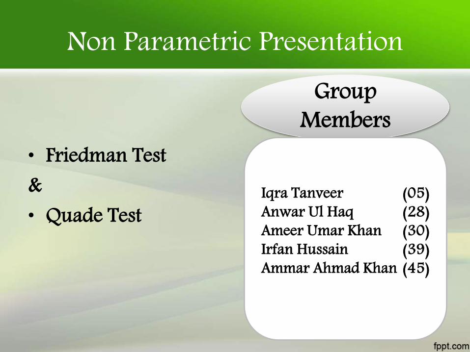
Non Parametric Presentation
• Friedman Test&• Quade Test
Group Members
Iqra Tanveer (05)Anwar Ul Haq (28)Ameer Umar Khan (30)Irfan Hussain (39)Ammar Ahmad Khan (45)

Learning Objectives• History• Introduction• Assumptions• General Procedure• Applications• Advantages• Disadvantages• Example

History• Friedman,
Milton (December 1937). • Friedman, Milton (March
1940).• “A comparison of
alternative tests of significance for the problem of m rankings“.
• Kendall, M. G. Rank Correlation Methods. (1970) London.

History• Hollander, M., and Wolfe, D. (1973). New
York.• Siegel, Sidney, and Castellan, N. John
Nonparametric Statistics for the Behavioral Sciences. (1988).
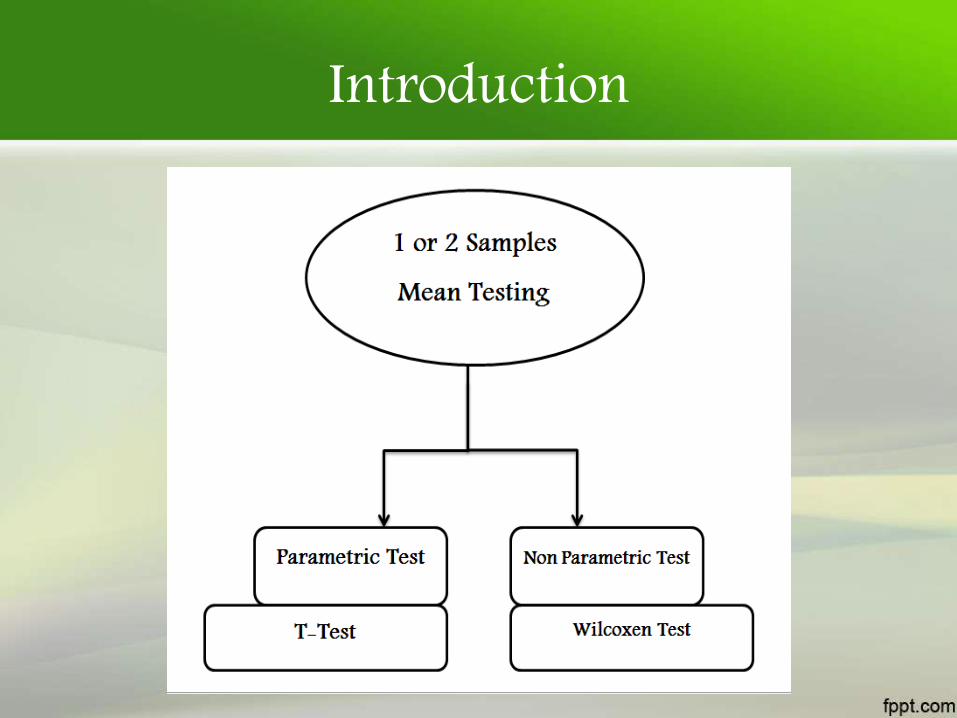
Introduction
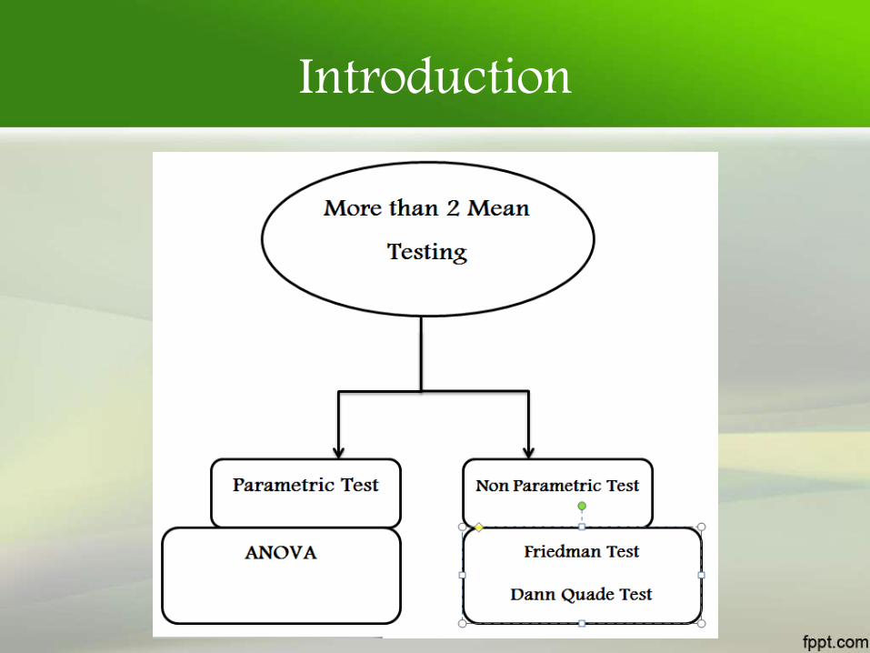
Introduction

Introduction
• The Friedman test is a non-parametric statisticaltest developed by the U.S. economist MiltonFriedman.
• Friedman test is a non-parametric randomizedblock analysis of variance.
• Similar to the parametric repeatedmeasures ANOVA. It is used to detect differencesin treatments across multiple test attempts.
Introduction• The procedure involves ranking each row
(or block) together, then considering the valuesof ranks by columns. Applicable to completeblock designs.
• It is thus a special case of the Durbin test.• The Friedman test is used for one-way repeated
measures analysis of variance by ranks. In its useof ranks it is similar to the Kruskal-Wallis one-way analysis of variance by ranks.

Introduction
• It is non-parametric test in which we use the f-table for critical region.
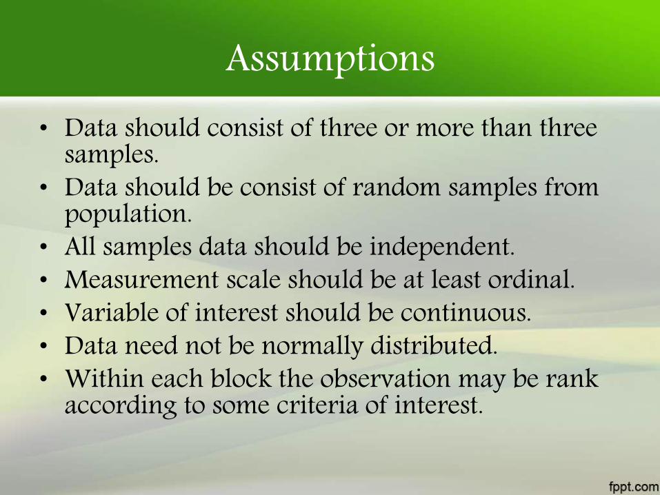
Assumptions• Data should consist of three or more than three
samples.• Data should be consist of random samples from
population.• All samples data should be independent. • Measurement scale should be at least ordinal.• Variable of interest should be continuous.• Data need not be normally distributed.• Within each block the observation may be rank
according to some criteria of interest.

General Procedure
1. Null & Alternative Hypothesis.Ho: The distributions (whatever they are)
are the same across repeated measures.H1: The distributions across repeated
measures are different.2. Level Of Significance.
α = 0.01, 0.05, 0.01…. (chose as required
for test)

General Procedure
3. Test StatisticsStep 1If no ties occur in data.
T1 =12
bk(k + 1)
j=1
k
Rj −b(k + 1)
2
2
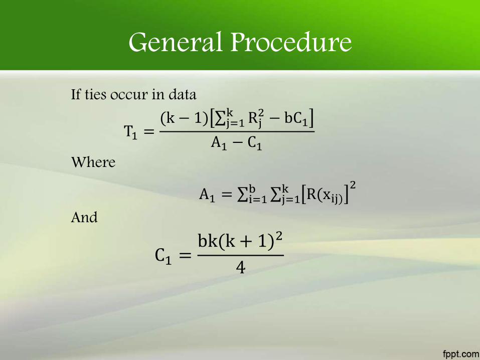
General ProcedureIf ties occur in data
T1 =(k − 1) j=1
k Rj2 − bC1
A1 − C1Where
A1 = i=1b j=1
k R(xij)2
And
C1 =bk(k + 1)2
4

General ProcedureStep 2
Put the value of 𝑇1 into this equation
𝑇2 =(𝑏−1)𝑇1
𝑏(𝑘−1)𝑇1
Where 𝑇2 ↝ 𝐹 𝑘1, 𝑘2 𝛼And𝑘1=k-1
𝑘2=(k-1)(b-1)
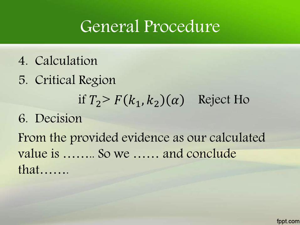
General Procedure4. Calculation5. Critical Region
if 𝑇2> 𝐹 𝑘1, 𝑘2 𝛼 Reject Ho6. DecisionFrom the provided evidence as our calculated value is …….. So we …… and conclude that…….

ApplicationsThis can be used to perform the testing in every field, where comparison between variables is required.1. Used to compare the effects of same fertilizer in
different patches of field having different fertility levels. (In agricultural Field)
2. Comparison between different companies cold drinks.
3. Test the equality of difference car’s engines performance. (In industries)
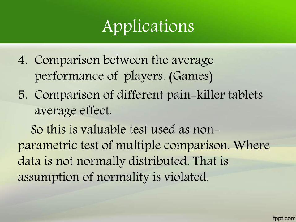
Applications4. Comparison between the average
performance of players. (Games)5. Comparison of different pain-killer tablets
average effect.So this is valuable test used as non-
parametric test of multiple comparison. Where data is not normally distributed. That is assumption of normality is violated.

Advantages
1. Since the Friedman test ranks the values in each row, it is not affected by sources of variability that equally affect all values in a row (since that factor won't change the ranks within the row).
2. The test controls experimental variability between subjects, thus increasing the power of the test.

Disadvantage
• Since this test does not make a distribution assumption, it is not as powerful as the ANOVA.

ExampleA B C D4 3 2 14 2 3 13 1.5 1.5 43 1 2 44 2 1 32 2 2 41 3 2 42 4 1 3
3.5 1 2 3.54 1 3 24 2 3 1
3.5 1 2 3.538 23.5 34.5 30
Ranked Data

Solution1. Null & Alternative Hypothesis.
Ho: The distributions (whatever they are) are the same across repeated measures.H1: The distributions across repeated measures are different.
2. Level Of Significance.α=0.05
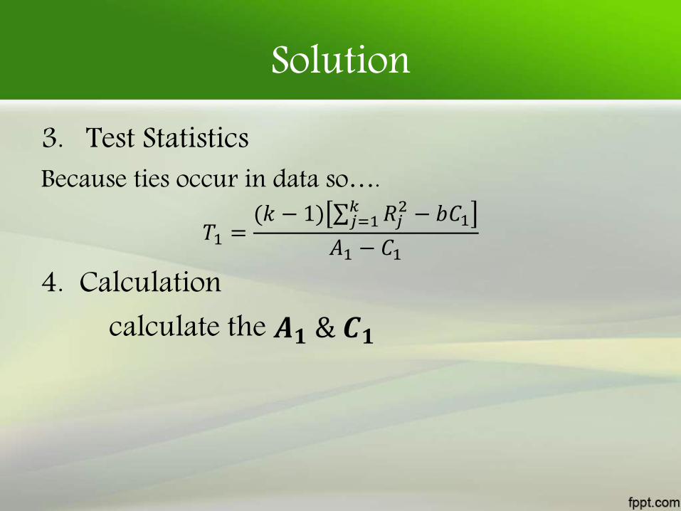
Solution3. Test StatisticsBecause ties occur in data so….
𝑇1 =(𝑘 − 1) 𝑗=1
𝑘 𝑅𝑗2 − 𝑏𝐶1
𝐴1 − 𝐶1
4. Calculationcalculate the 𝑨𝟏 & 𝑪𝟏

SolutionAs we know that:
𝐴1 =
𝑖=1
𝑏
𝑗=1
𝑘
𝑅(𝑥𝑖𝑗)2
And
𝐶1 =𝑏𝑘(𝑘+1)2
4
By using these formulas we calculate that𝐴1=456.5 𝐶1=300
Solution
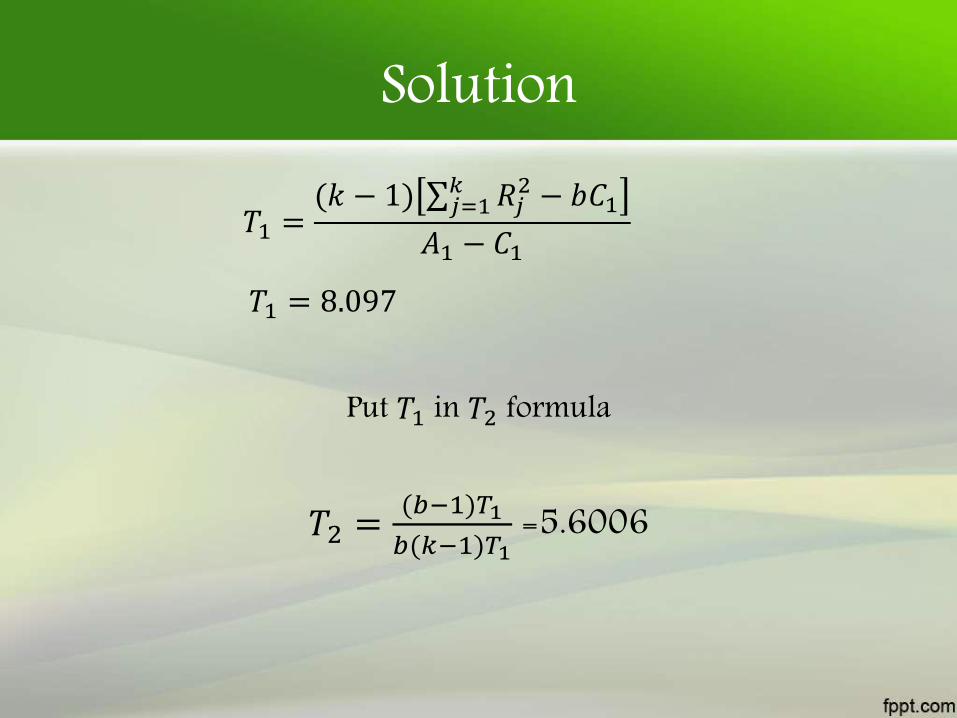
𝑇1 =(𝑘 − 1) 𝑗=1
𝑘 𝑅𝑗2 − 𝑏𝐶1
𝐴1 − 𝐶1
𝑇1 = 8.097
Put 𝑇1 in 𝑇2 formula
𝑇2 =(𝑏−1)𝑇1
𝑏(𝑘−1)𝑇1=5.6006
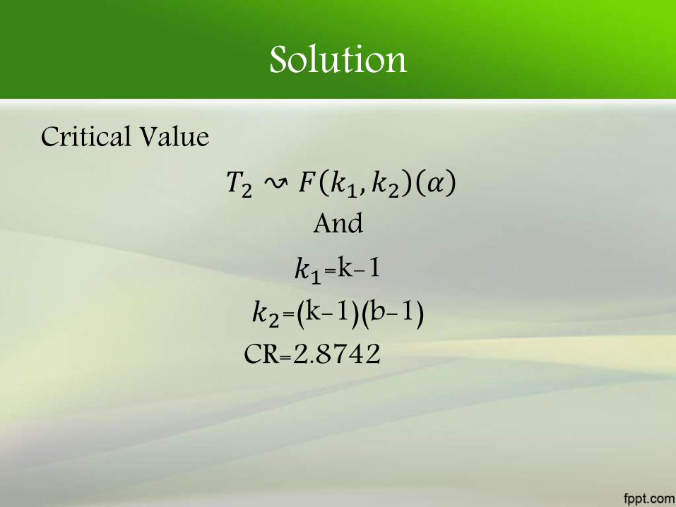
SolutionCritical Value
𝑇2 ↝ 𝐹 𝑘1, 𝑘2 𝛼
And𝑘1=k-1
𝑘2=(k-1)(b-1)CR=2.8742
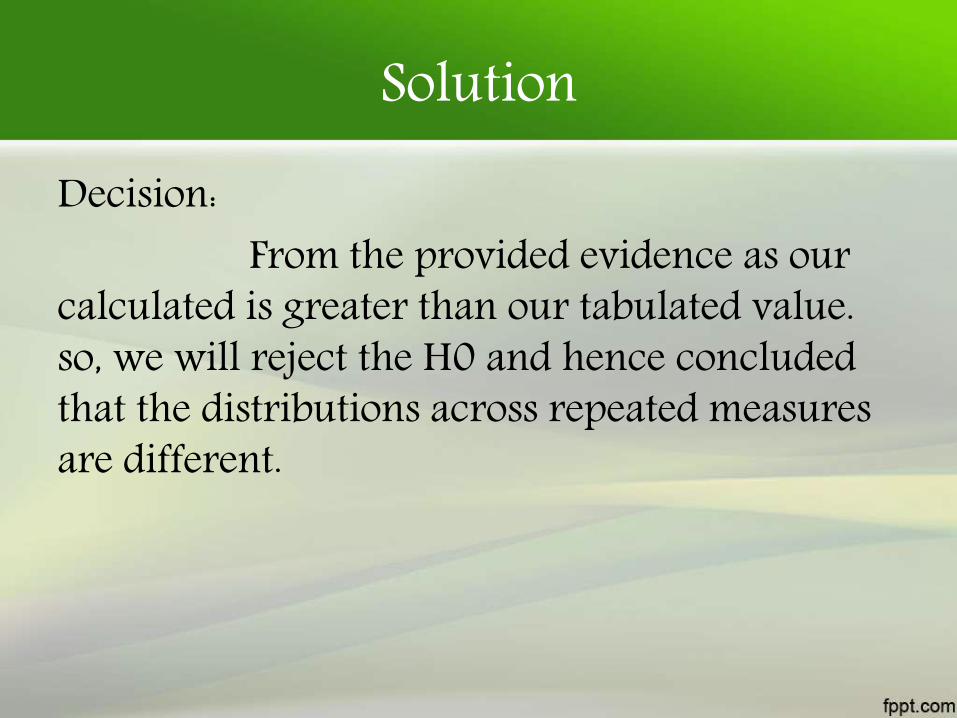
SolutionDecision:
From the provided evidence as our calculated is greater than our tabulated value. so, we will reject the H0 and hence concluded that the distributions across repeated measures are different.
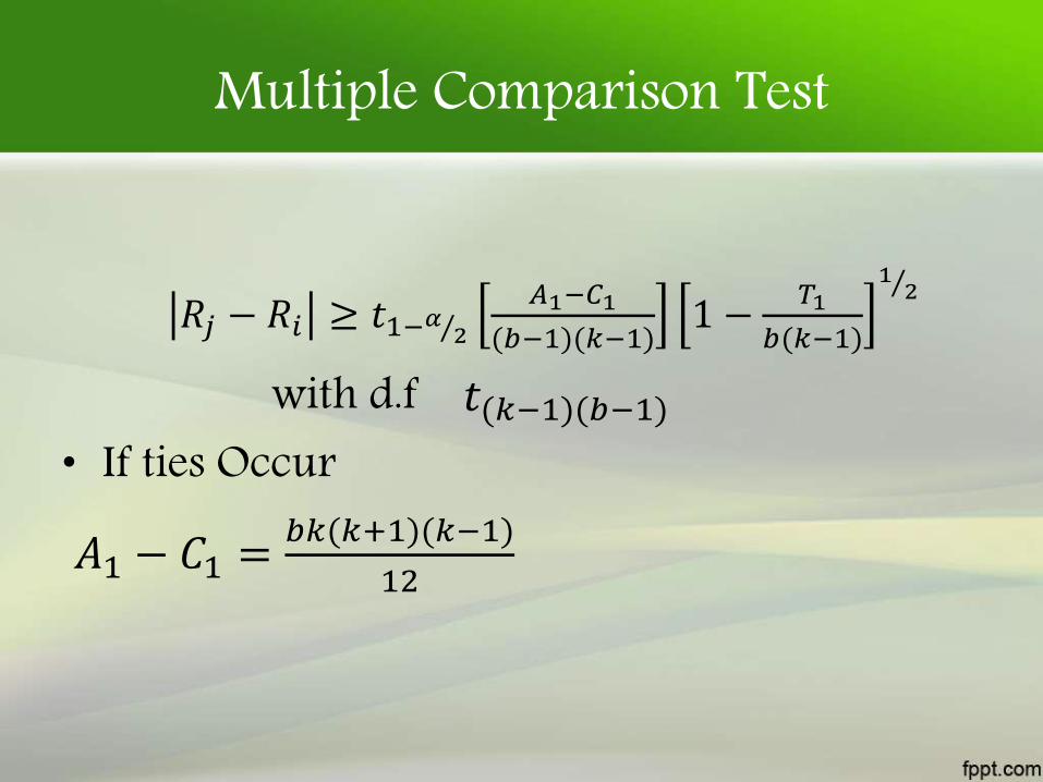
Multiple Comparison Test
𝑅𝑗 − 𝑅𝑖 ≥ 𝑡1− 𝛼 2𝐴1−𝐶1
(𝑏−1)(𝑘−1)1 −
𝑇1
𝑏(𝑘−1)
1 2
with d.f 𝑡(𝑘−1)(𝑏−1)• If ties Occur
𝐴1 − 𝐶1 =𝑏𝑘(𝑘+1)(𝑘−1)
12