33
Forecasting Techniques Part 2

7/27/2019 Presentation - Session 10
http://slidepdf.com/reader/full/presentation-session-10 1/33
Forecasting Techniques
Part 2

7/27/2019 Presentation - Session 10
http://slidepdf.com/reader/full/presentation-session-10 2/33
© Copyright Coleago 2010
Learning Objectives
ExplanatoryMethods
How to use explanatory methods, notably regressionanalysis to make a forecast
Curve Fitting Using the product life cycle and s-shaped growth
curves to forecast take-up
Diffusion of
Innovation
The Bass model of diffusion of innovation to forecast
new demand for new services
Price Elasticity
of Demand
Price elasticity of demand in telecoms markets,
practical applications
1

7/27/2019 Presentation - Session 10
http://slidepdf.com/reader/full/presentation-session-10 3/33
© Copyright Coleago 2010
Learning Objectives
ExplanatoryMethods
How to use explanatory methods, notably regressionanalysis to make a forecast
Curve Fitting Using the product life cycle and s-shaped growth
curves to forecast take-up
Diffusion of
Innovation
The Bass model of diffusion of innovation to forecast
new demand for new services
Price Elasticity
of Demand
Price elasticity of demand in telecoms markets,
practical applications
2
7/27/2019 Presentation - Session 10
http://slidepdf.com/reader/full/presentation-session-10 4/33
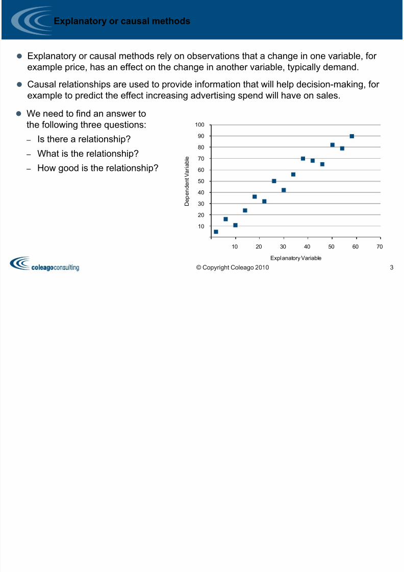
Explanatory or causal methods
Explanatory or causal methods rely on observations that a change in one variable, for
example price, has an effect on the change in another variable, typically demand. Causal relationships are used to provide information that will help decision-making, for
example to predict the effect increasing advertising spend will have on sales.
We need to find an answer to
the following three questions:
– Is there a relationship? – What is the relationship?
– How good is the relationship?
10
20
30
40
50
60
70
80
90
100
10 20 30 40 50 60 70
D e p e n d e n t V a r i a b l e
Explanatory Variable
© Copyright Coleago 2010 3
7/27/2019 Presentation - Session 10
http://slidepdf.com/reader/full/presentation-session-10 5/33
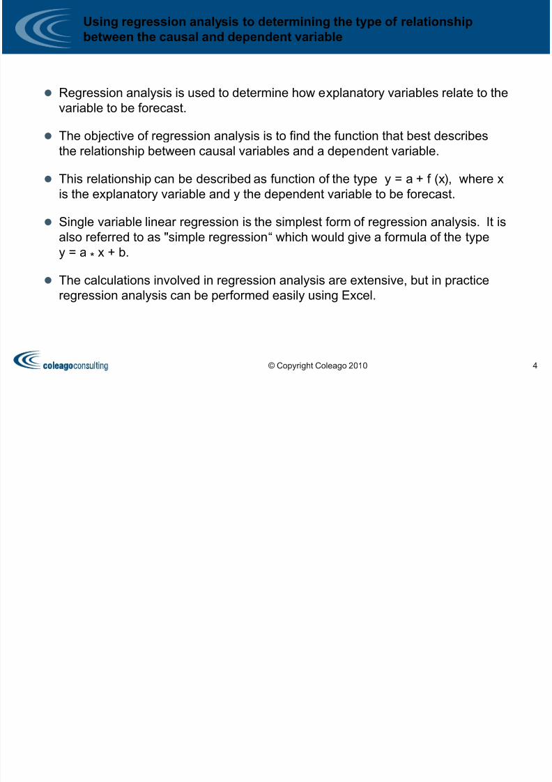
Using regression analysis to determining the type of relationship
between the causal and dependent variable
Regression analysis is used to determine how explanatory variables relate to thevariable to be forecast.
The objective of regression analysis is to find the function that best describes
the relationship between causal variables and a dependent variable.
This relationship can be described as function of the type y = a + f (x), where x
is the explanatory variable and y the dependent variable to be forecast.
Single variable linear regression is the simplest form of regression analysis. It is
also referred to as "simple regression“ which would give a formula of the type
y = a * x + b.
The calculations involved in regression analysis are extensive, but in practice
regression analysis can be performed easily using Excel.
© Copyright Coleago 2010 4
7/27/2019 Presentation - Session 10
http://slidepdf.com/reader/full/presentation-session-10 6/33
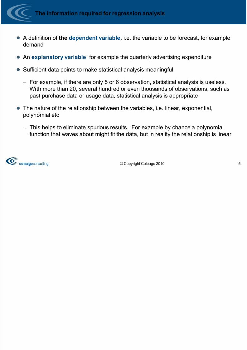
The information required for regression analysis
A definition of the dependent variable, i.e. the variable to be forecast, for example
demand
An explanatory variable, for example the quarterly advertising expenditure
Sufficient data points to make statistical analysis meaningful
– For example, if there are only 5 or 6 observation, statistical analysis is useless.
With more than 20, several hundred or even thousands of observations, such as
past purchase data or usage data, statistical analysis is appropriate
The nature of the relationship between the variables, i.e. linear, exponential,
polynomial etc
– This helps to eliminate spurious results. For example by chance a polynomialfunction that waves about might fit the data, but in reality the relationship is linear
© Copyright Coleago 2010 5

7/27/2019 Presentation - Session 10
http://slidepdf.com/reader/full/presentation-session-10 7/33
Two outputs from a regression analysis
A function or formula that describes the relationships between the explanatoryvariables and the dependent variable
– This formula can be readily used in spreadsheets for the purposes of
forecasting.
A measure of goodness of fit, i.e. how well the function fits the observed data
– As with time series analysis, some of the variation in the observed data will be
due to random events, i.e. error. Producing a good fit means minimising
error.
© Copyright Coleago 2010 6
7/27/2019 Presentation - Session 10
http://slidepdf.com/reader/full/presentation-session-10 8/33
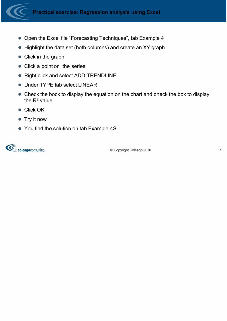
Practical exercise: Regression analysis using Excel
Open the Excel file “Forecasting Techniques”, tab Example 4 Highlight the data set (both columns) and create an XY graph
Click in the graph
Click a point on the series
Right click and select ADD TRENDLINE
Under TYPE tab select LINEAR
Check the bock to display the equation on the chart and check the box to display
the R2 value
Click OK
Try it now
You find the solution on tab Example 4S
© Copyright Coleago 2010 7
7/27/2019 Presentation - Session 10
http://slidepdf.com/reader/full/presentation-session-10 9/33
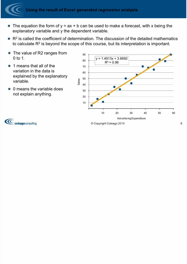
Using the result of Excel generated regression analysis
The equation the form of y = ax + b can be used to make a forecast, with x being the
explanatory variable and y the dependent variable. R2 is called the coefficient of determination. The discussion of the detailed mathematics
to calculate R2 is beyond the scope of this course, but its interpretation is important.
The value of R2 ranges from
0 to 1.
1 means that all of thevariation in the data is
explained by the explanatory
variable.
0 means the variable does
not explain anything.
y = 1.4913x + 3.6692R² = 0.96
10
20
30
40
50
60
70
80
90
10 20 30 40 50 60
S a l e s
Advertis ing Expenditure
© Copyright Coleago 2010 8
7/27/2019 Presentation - Session 10
http://slidepdf.com/reader/full/presentation-session-10 10/33
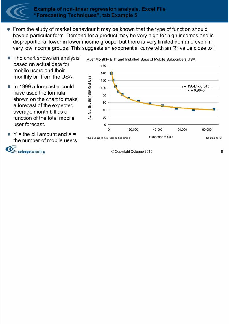
Example of non-linear regression analysis. Excel File
“Forecasting Techniques”, tab Example 5
From the study of market behaviour it may be known that the type of function should
have a particular form. Demand for a product may be very high for high incomes and is
disproportional lower in lower income groups, but there is very limited demand even invery low income groups. This suggests an exponential curve with an R2 value close to 1.
The chart shows an analysis
based on actual data for
mobile users and their
monthly bill from the USA.
In 1999 a forecaster could
have used the formula
shown on the chart to make
a forecast of the expected
average month bill as a
function of the total mobileuser forecast.
Y = the bill amount and X =
the number of mobile users.
y = 1964.1x-0.343R² = 0.9943
0
20
40
60
80
100
120
140
160
0 20,000 40,000 60,000 80,000
A v . M o n t h l y B i l l 1 9 9 9 R e a l U
S $
Subscribers '000
Aver Monthly Bill* and Installed Base of Mobile Subscribers USA
* Excluding long distance & roaming Source: CTIA
© Copyright Coleago 2010 9

7/27/2019 Presentation - Session 10
http://slidepdf.com/reader/full/presentation-session-10 11/33
© Copyright Coleago 2010
Learning Objectives
ExplanatoryMethods
How to use explanatory methods, notably regressionanalysis to make a forecast
Curve Fitting Using the product life cycle and s-shaped growth
curves to forecast take-up
Diffusion of
Innovation
The Bass model of diffusion of innovation to forecast
new demand for new services
Price Elasticity
of Demand
Price elasticity of demand in telecoms markets,
practical applications
10

7/27/2019 Presentation - Session 10
http://slidepdf.com/reader/full/presentation-session-10 12/33
Market behaviour models: an overview
Economics and business studies provide a wealth of empirical data. From the
study of how markets, competitors and prices behave, a number of generallyaccepted models have emerged.
– Examples are the product life cycle, diffusion of innovation etc.
These models are similar to the laws of natural science and provide a useful tool
box for the forecaster.
Market behaviour models fall into the category of qualitative forecast methods.
Market behaviour models share similarities with time series and causal models,
because they explain what happens over time and how different factors are
related.
– For example, price elasticity is an observation that describes how demand
reacts to price and it may be possible to determine the price elasticity
coefficient using regression analysis.
© Copyright Coleago 2010 11
7/27/2019 Presentation - Session 10
http://slidepdf.com/reader/full/presentation-session-10 13/33
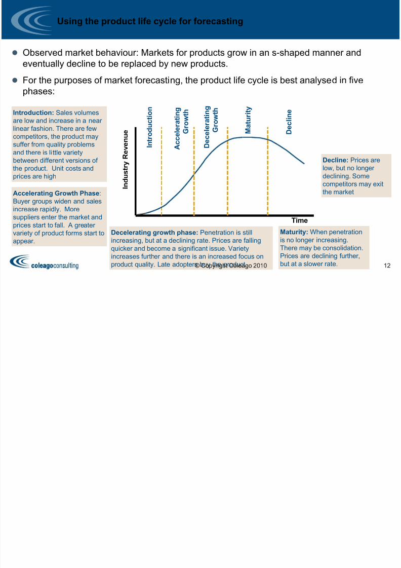
Using the product life cycle for forecasting
Observed market behaviour: Markets for products grow in an s-shaped manner and
eventually decline to be replaced by new products.
For the purposes of market forecasting, the product life cycle is best analysed in five
phases:
Introduction: Sales volumes
are low and increase in a near
linear fashion. There are few
competitors, the product may
suffer from quality problems
and there is li ttle variety
between different versions of
the product. Unit costs and
prices are high
Accelerating Growth Phase:
Buyer groups widen and sales
increase rapidly. Moresuppliers enter the market and
prices start to fall. A greater
variety of product forms start to
appear.
Decelerating growth phase: Penetration is still
increasing, but at a declining rate. Prices are falling
quicker and become a significant issue. Variety
increases further and there is an increased focus on
product quality. Late adopters buy the product.
Maturity: When penetration
is no longer increasing.
There may be consolidation.
Prices are declining further,
but at a slower rate.
Decline: Prices are
low, but no longer
declining. Some
competitors may exit
the market
I n t r o d u c t i o n
A c c e l e r a t i n g
G r o w t h
M a t u r i t y
D e c l i n e
Time
I n d u s t r y R e v e n
u e
D e
c e l e r a t i n g
G r o w t h
© Copyright Coleago 2010 12
7/27/2019 Presentation - Session 10
http://slidepdf.com/reader/full/presentation-session-10 14/33
0
200
400
600
800
1,000
1,200
1,400
1,600
1,800
1 9 9 8
2 0 0 0
2 0 0 2
2 0 0 4
2 0 0 6
2 0 0 8
2 0 1 0
2 0 1 2
2 0 1 4
2 0 1 6
2 0 1 8
M o b i l e U s e
r s ' 0 0 0
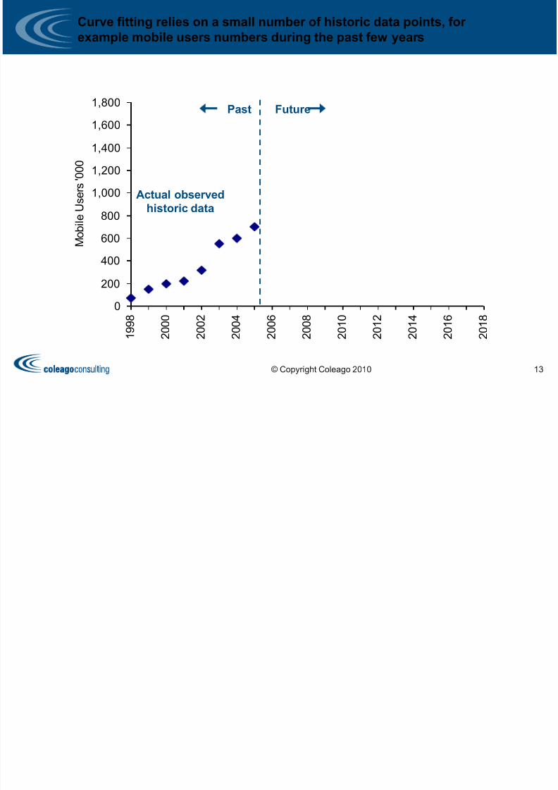
Curve fitting relies on a small number of historic data points, for
example mobile users numbers during the past few years
Actual observedhistoric data
Past Future
© Copyright Coleago 2010 13
7/27/2019 Presentation - Session 10
http://slidepdf.com/reader/full/presentation-session-10 15/33
0
200
400
600
800
1,000
1,200
1,400
1,600
1,800
1 9 9 8
2 0 0 0
2 0 0 2
2 0 0 4
2 0 0 6
2 0 0 8
2 0 1 0
2 0 1 2
2 0 1 4
2 0 1 6
2 0 1 8
M o b i l e U s e
r s ' 0 0 0
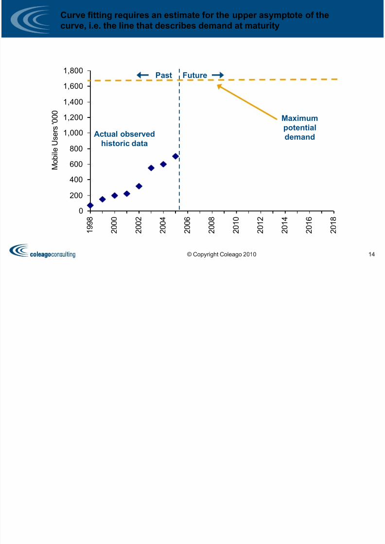
Curve fitting requires an estimate for the upper asymptote of the
curve, i.e. the line that describes demand at maturity
Actual observedhistoric data
Past Future
Maximum
potential
demand
© Copyright Coleago 2010 14
7/27/2019 Presentation - Session 10
http://slidepdf.com/reader/full/presentation-session-10 16/33
0
200
400
600
800
1,000
1,200
1,400
1,600
1,800
1 9 9 8
2 0 0 0
2 0 0 2
2 0 0 4
2 0 0 6
2 0 0 8
2 0 1 0
2 0 1 2
2 0 1 4
2 0 1 6
2 0 1 8
M o b i l e U s e
r s ' 0 0 0
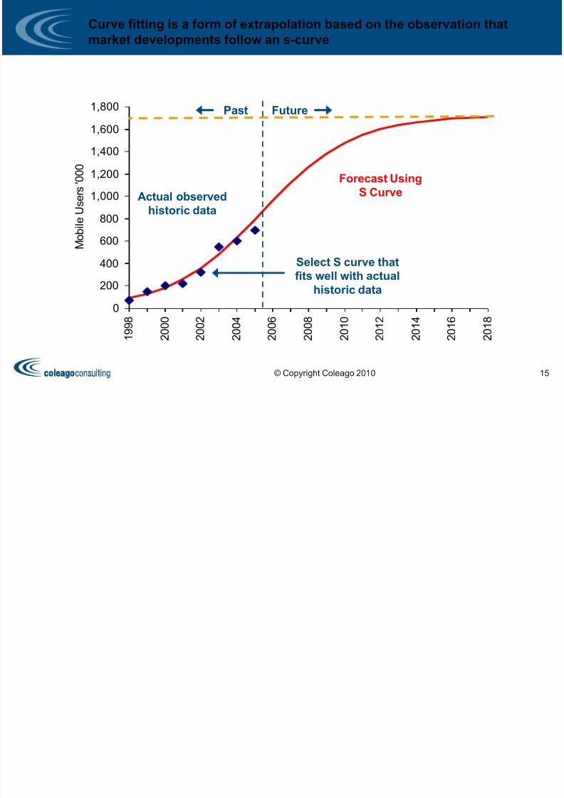
Curve fitting is a form of extrapolation based on the observation that
market developments follow an s-curve
Actual observedhistoric data
Past Future
Forecast Using
S Curve
Select S curve that
fits well with actual
historic data
© Copyright Coleago 2010 15

7/27/2019 Presentation - Session 10
http://slidepdf.com/reader/full/presentation-session-10 17/33
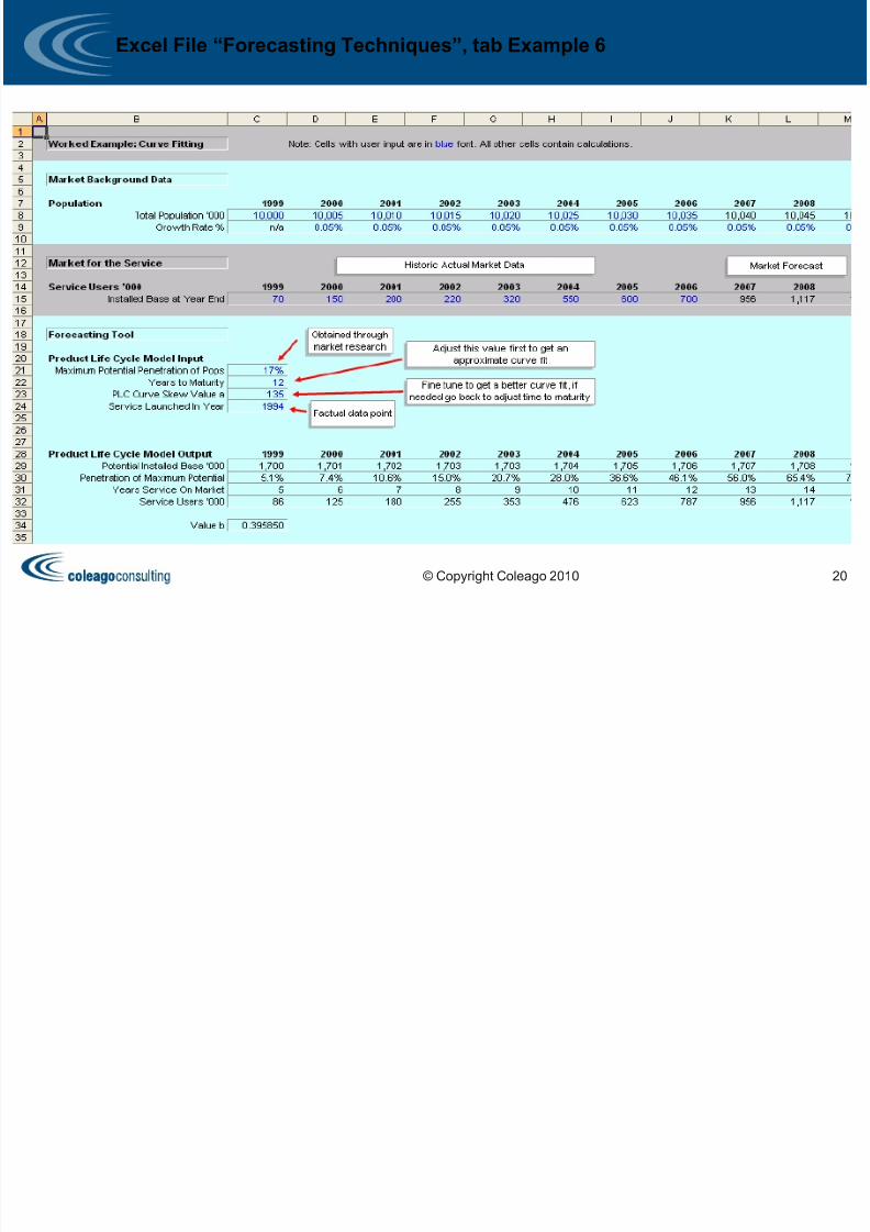
Pearl’s equation can be used in a practical manner to produce an s-curve
yt = m * ( 1 / (1 + a * e^ (-b * t)))
where
yt = the penetration in year t
m = the demand at maturity
a = a factor giving more / less growth later or earlier, the neutral value is 99
t = number of years after launch
b = a factor shortening or lengthening the time to maturity (calculated, see
below)
b = 1 / T * ( ln ( a / ( 1/0.99 - 1)))
where
a = a factor giving more / less growth later or earlier, the neutral value is 99
T = the total years to maturity
© Copyright Coleago 2010 16

7/27/2019 Presentation - Session 10
http://slidepdf.com/reader/full/presentation-session-10 18/33
Fitting the curve
The essence of curve fitting is to select a particular s-curve that fits well with the
historic data points.
Assuming you have determined the maximum potential demand, i.e. the
demand at maturity, you now have to vary in the s-curve formula the values for
the parameters
– A (the curve skew value) to give more or less growth earlier or later
– And the time to maturity, fore example the number of years.
The effect of varying the curve skew value a and the time to maturity is show on
the following two slides.
© Copyright Coleago 2010 17
7/27/2019 Presentation - Session 10
http://slidepdf.com/reader/full/presentation-session-10 19/33
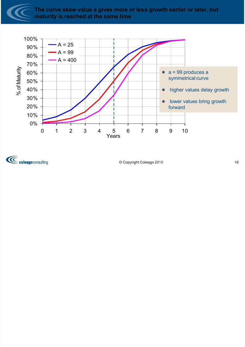
The curve skew value a gives more or less growth earlier or later, but
maturity is reached at the same time
0%
10%
20%
30%
40%
50%
60%
70%
80%
90%
100%
0 1 2 3 4 5 6 7 8 9 10Years
% o
f M a t u r i t y
A = 25 A = 99
A = 400
a = 99 produces a
symmetrical curve
higher values delay growth
lower values bring growth
forward
© Copyright Coleago 2010 18
Th ti t t it b l th d h t d b i th
7/27/2019 Presentation - Session 10
http://slidepdf.com/reader/full/presentation-session-10 20/33
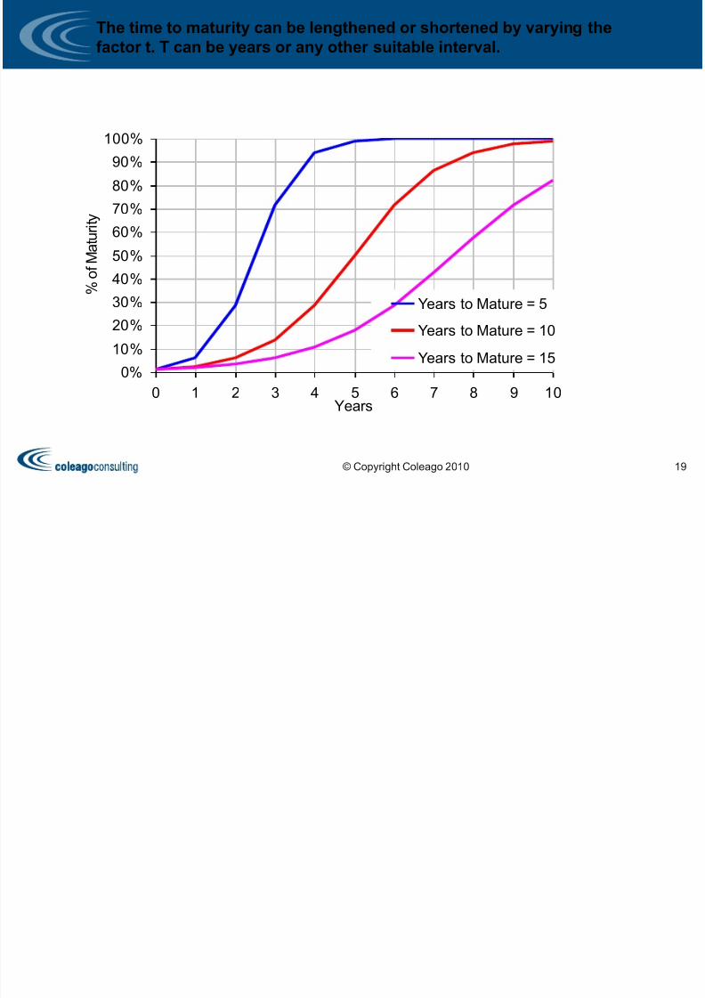
The time to maturity can be lengthened or shortened by varying the
factor t. T can be years or any other suitable interval.
0%
10%
20%
30%
40%
50%
60%
70%
80%
90%
100%
0 1 2 3 4 5 6 7 8 9 10Years
% o
f M a
t u r i t y
Years to Mature = 5
Years to Mature = 10
Years to Mature = 15
© Copyright Coleago 2010 19
7/27/2019 Presentation - Session 10
http://slidepdf.com/reader/full/presentation-session-10 21/33
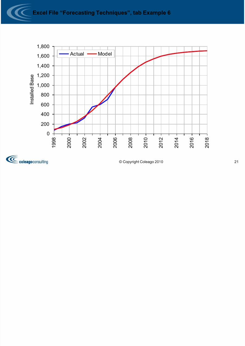
Excel File “Forecasting Techniques”, tab Example 6
© Copyright Coleago 2010 20
7/27/2019 Presentation - Session 10
http://slidepdf.com/reader/full/presentation-session-10 22/33
Excel File “Forecasting Techniques”, tab Example 6
0
200
400
600
8001,000
1,200
1,400
1,600
1,800
1 9 9 8
2 0 0 0
2 0 0 2
2 0 0 4
2 0 0 6
2 0 0 8
2 0 1 0
2 0 1 2
2 0 1 4
2 0 1 6
2 0 1 8
I n s t a l l e d
B a s e
Actual Model
© Copyright Coleago 2010 21

7/27/2019 Presentation - Session 10
http://slidepdf.com/reader/full/presentation-session-10 23/33
© Copyright Coleago 2010
Learning Objectives
Explanatory
Methods
How to use explanatory methods, notably regression
analysis to make a forecast
Curve Fitting Using the product life cycle and s-shaped growth
curves to forecast take-up
Diffusion of Innovation
The Bass model of diffusion of innovation to forecastnew demand for new services
Price Elasticity
of Demand
Price elasticity of demand in telecoms markets,
practical applications
22
7/27/2019 Presentation - Session 10
http://slidepdf.com/reader/full/presentation-session-10 24/33
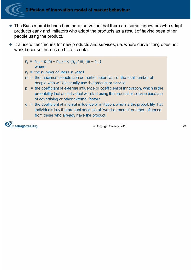
Diffusion of innovation model of market behaviour
The Bass model is based on the observation that there are some innovators who adopt
products early and imitators who adopt the products as a result of having seen other
people using the product.
It a useful techniques for new products and services, i.e. where curve fitting does not
work because there is no historic data
nt = nt-1 + p (m – nt-1) + q (nt-1 / m) (m – nt-1)
where:nt = the number of users in year t
m = the maximum penetration or market potential, i.e. the total number of
people who will eventually use the product or service
p = the coefficient of external influence or coefficient of innovation, which is the
probability that an individual will start using the product or service because
of advertising or other external factors
q = the coefficient of internal influence or imitation, which is the probability that
individuals buy the product because of "word-of-mouth" or other influence
from those who already have the product.
© Copyright Coleago 2010 23
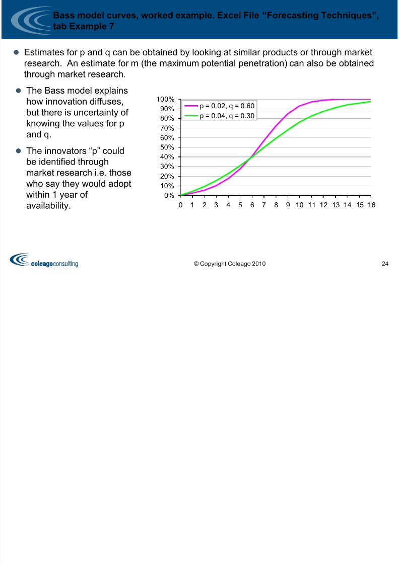
Bass model curves worked example Excel File “Forecasting Techniques”
7/27/2019 Presentation - Session 10
http://slidepdf.com/reader/full/presentation-session-10 25/33
Bass model curves, worked example. Excel File Forecasting Techniques ,
tab Example 7
Estimates for p and q can be obtained by looking at similar products or through market
research. An estimate for m (the maximum potential penetration) can also be obtained
through market research.
The Bass model explains
how innovation diffuses,
but there is uncertainty of
knowing the values for p
and q.
The innovators “p” could
be identified through
market research i.e. those
who say they would adopt
within 1 year of
availability.
0%
10%
20%
30%
40%
50%
60%
70%
80%
90%
100%
0 1 2 3 4 5 6 7 8 9 10 11 12 13 14 15 16
p = 0.02, q = 0.60
p = 0.04, q = 0.30
© Copyright Coleago 2010 24
The speed of diffusion of innovation varies between countries and is

7/27/2019 Presentation - Session 10
http://slidepdf.com/reader/full/presentation-session-10 26/33
The speed of diffusion of innovation varies between countries and is
similar for different products within the same country
A recent study found that the speed diffusion of innovation varies between
countries depending on the cultural factors. Detailed insight is provided by the
research findings published by Trellis, Stremersch and Yin 1.
This shows that time to take-off varies, among other things, substantially by
country. In Scandinavian countries time to take-off was almost as half long as in
Mediterranean countries. The mobile market does not appear to be an
exception to this.
In order to gain insight into the speed of adoption of a new services, apart from
looking at market research you might analyse diffusion curves of other
technology services and products or other consumer products in your country.
1) Trellis, Stremersch and Yin; “The International Takeoff of New Products: The Role of Economics,
Culture, and Country Innovativeness”, Marketing Science, Vol. 22 No. 2, Spring 2003, pp 188-208.
The research paper is included in the course pack.
© Copyright Coleago 2010 25
C l i f “Th I t t i l T k Off f N P d t ”

7/27/2019 Presentation - Session 10
http://slidepdf.com/reader/full/presentation-session-10 27/33
Conclusions from “The Internat ional Take-Off of New Produ cts ”
Products take-off faster in wealthier countries than in poorer countries
Products take-off faster in industrious countries
Products take-off faster in high media intensity countries
Products take-off faster in highly educated economies
PC and Internet penetration would be an interesting new variable to include in
the analysis
© Copyright Coleago 2010 26
L i Obj ti

7/27/2019 Presentation - Session 10
http://slidepdf.com/reader/full/presentation-session-10 28/33
© Copyright Coleago 2010
Learning Objectives
Explanatory
Methods
How to use explanatory methods, notably regression
analysis to make a forecast
Curve Fitting Using the product life cycle and s-shaped growth
curves to forecast take-up
Diffusion of Innovation
The Bass model of diffusion of innovation to forecastnew demand for new services
Price Elasticity
of Demand
Price elasticity of demand in telecoms markets,
practical applications
27
D d l ti iti

7/27/2019 Presentation - Session 10
http://slidepdf.com/reader/full/presentation-session-10 29/33
Demand elasticities
Elasticities are a measure of how a change in a variable affects demand.
There are many different types of elasticities:
– price elasticity of demand
– cross price elasticity of demand
– income elasticity of demand
– elasticity to advertising expenditure
– etc…..
© Copyright Coleago 2010 28
In the context of market forecasting the most important elasticity is
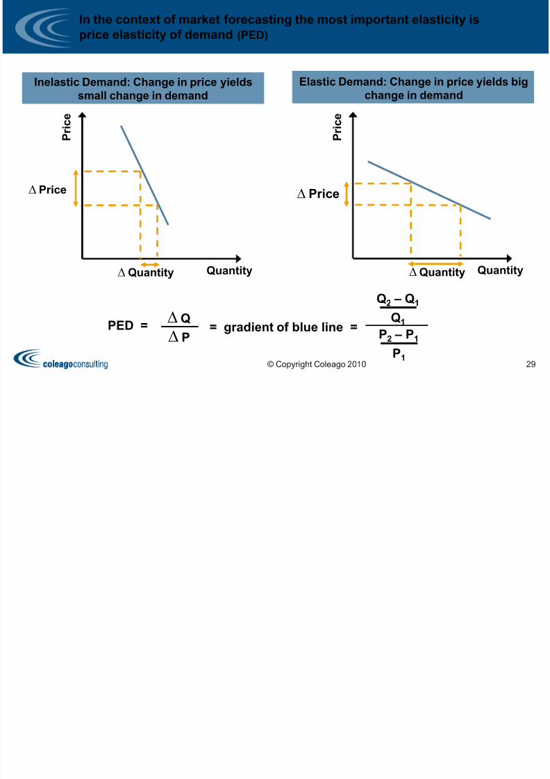
7/27/2019 Presentation - Session 10
http://slidepdf.com/reader/full/presentation-session-10 30/33
price elasticity of demand (PED)
Quantity
P r i c e
∆ Price
∆ Quantity
Inelastic Demand: Change in price yields
small change in demand
Quantity
P r i c e
∆ Price
∆ Quantity
Elastic Demand: Change in price yields big
change in demand
PED =∆ Q
∆ P= gradient of blue line =
Q2 – Q1
Q1
P2 – P1
P1© Copyright Coleago 2010 29
In practice elasticities have to be estimated rather than measured

7/27/2019 Presentation - Session 10
http://slidepdf.com/reader/full/presentation-session-10 31/33
In practice elasticities have to be estimated rather than measured
It is unlikely that the there is no effect on demand if prices change, i.e. the price
elasticity coefficient is unlikely to be 0.
Equally, it is unlikely that if prices decline, demand increases in exactly the same
proportion, i.e. the price elasticity coefficient is unlikely to be -1.
Studies have produced estimates for price elasticity coefficients in telecoms market
ranging from:
– - 0.8 for international calls
– to - 0.1 for local calls
Elasticities are generally not constant. The law of diminishing return applies, e.g. if
prices fall to zero demand would be infinite.
If prices are very low in the context of the expenditure of an individual, changes in
price will have little effect on demand, i.e. the price elasticity coefficient is close to 0.
© Copyright Coleago 2010 30
In any forecast it is good practice to use price elasticity explicitly
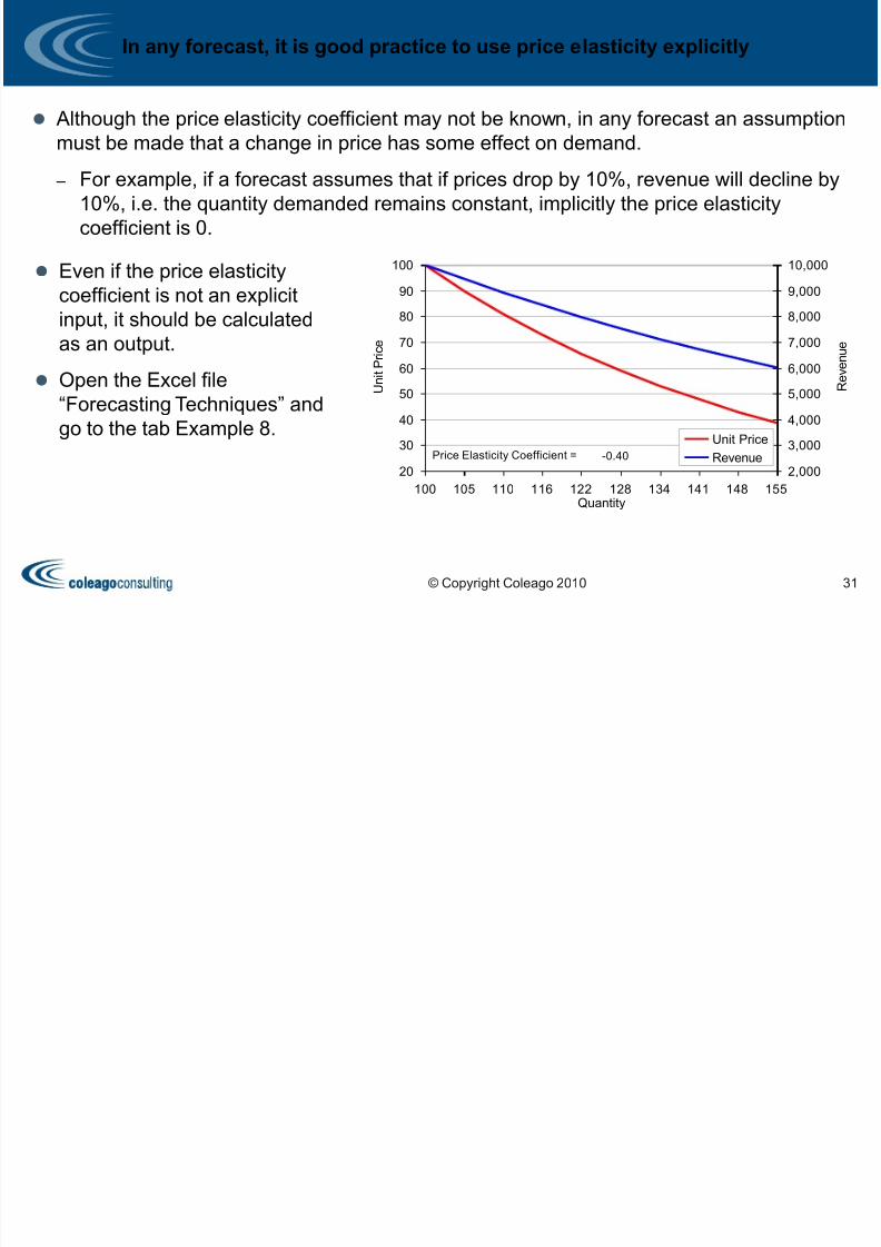
7/27/2019 Presentation - Session 10
http://slidepdf.com/reader/full/presentation-session-10 32/33
In any forecast, it is good practice to use price elasticity explicitly
Although the price elasticity coefficient may not be known, in any forecast an assumption
must be made that a change in price has some effect on demand.
– For example, if a forecast assumes that if prices drop by 10%, revenue will decline by
10%, i.e. the quantity demanded remains constant, implicitly the price elasticity
coefficient is 0.
Even if the price elasticity
coefficient is not an explicit
input, it should be calculatedas an output.
Open the Excel file
“Forecasting Techniques” and
go to the tab Example 8.
20
30
40
50
60
70
80
90
100
100 105 110 116 122 128 134 141 148 155Quantity
U n i t P r i c e
2,000
3,000
4,000
5,000
6,000
7,000
8,000
9,000
10,000
R e v e n u e
Unit Price
RevenuePrice Elasticity Coefficient = -0.40
© Copyright Coleago 2010 31

7/27/2019 Presentation - Session 10
http://slidepdf.com/reader/full/presentation-session-10 33/33
Session Summary


