PRESERVING PRIVACY IN WIRELESS NETWORKS By Taojun Wu Thesis Submitted to the

PRESERVING PRIVACY IN WIRELESS NETWORKS

By

Taojun Wu

Thesis

Submitted to the Faculty of the

Graduate School of Vanderbilt University

in partial fulfillment of the requirements

for the degree of

MASTER OF SCIENCE

in

Computer Science

August, 2007

Nashville, Tennessee

Approved:

Professor Yuan Xue

Professor Lawrence W. Dowdy

ACKNOWLEDGMENTS

This work was supported in part by TRUST (The Team for Researchin Ubiquitous Secure

Technology), which receives support from the National Science Foundation (NSF award num-

ber CCF-0424422) and the following organizations: Cisco, ESCHER, HP, IBM, Intel, Microsoft,

ORNL, Pirelli, Qualcomm, Sun, Symantec, Telecom Italia and United Technologies.

I am especially indebted to Dr. Yuan Xue and Dr. Yi Cui for theirguidance, help, and patience

with me. Their constant encouragement was instrumental in keeping me motivated in the right

direction. I value their systematic academic training, which helped sharpening my critical thinking.

More importantly, their devoted mentoring was essential for my graduate study and the completion

of this thesis.

Dr. Gautam Biswas, Dr. Larry Dowdy, and Dr. Jerry Spinrad, andother faculty members of

EECS, Vanderbilt University, deserve my thanks for equipping me with advanced methodology

and supporting my past and future endeavors.

The members of VANETS and TRUST were sources of infinite help and entertainment. Thanks

to Bin, Liang, Yann, Nathan, and Jan.

Finally, I would like to thank my family for their support andencouragement.

ii

TABLE OF CONTENTS

Page

ACKNOWLEDGMENTS . . . . . . . . . . . . . . . . . . . . . . . . . . . . . . . . . . . . ii

LIST OF FIGURES . . . . . . . . . . . . . . . . . . . . . . . . . . . . . . . . . . . . . . .v

Chapter

I. INTRODUCTION . . . . . . . . . . . . . . . . . . . . . . . . . . . . . . . . . . 1

II. DIGITAL RIGHTS MANAGEMENT FOR WIRELESS NETWORKS . . . . . . 5

Introduction . . . . . . . . . . . . . . . . . . . . . . . . . . . . . . . . . . . . 5Overall DRM Framework . . . . . . . . . . . . . . . . . . . . . . . . . . . . 7Composite Wireless Networks Content Decomposition . . . . . . . .. . . . . 8Hierarchical Key Management and Data Encryption . . . . . . . . .. . . . . 10

Key Generation . . . . . . . . . . . . . . . . . . . . . . . . . . . . . . 10Encryption . . . . . . . . . . . . . . . . . . . . . . . . . . . . . . . . 12Access Control . . . . . . . . . . . . . . . . . . . . . . . . . . . . . . 12

Legal EU-Sensor Content Association . . . . . . . . . . . . . . . . . . . .. . 13Experimental Results . . . . . . . . . . . . . . . . . . . . . . . . . . . . . . . 16

Testbed Setup . . . . . . . . . . . . . . . . . . . . . . . . . . . . . . . 16Evaluation Results . . . . . . . . . . . . . . . . . . . . . . . . . . . . 17

Related Work . . . . . . . . . . . . . . . . . . . . . . . . . . . . . . . . . . . 18Conclusion . . . . . . . . . . . . . . . . . . . . . . . . . . . . . . . . . . . . 19

III. PRIVACY PRESERVATION IN WIRELESS MESH NETWORKS . . . . . . . . 20

Introduction . . . . . . . . . . . . . . . . . . . . . . . . . . . . . . . . . . . . 20Privacy Preserving Architecture . . . . . . . . . . . . . . . . . . . . . .. . . 23Privacy Modelling in WMN . . . . . . . . . . . . . . . . . . . . . . . . . . . 25

Network Model . . . . . . . . . . . . . . . . . . . . . . . . . . . . . . 25Traffic Entropy . . . . . . . . . . . . . . . . . . . . . . . . . . . . . . 26

Penalty-based Routing Algorithm . . . . . . . . . . . . . . . . . . . . . . .. 29Experimental Results . . . . . . . . . . . . . . . . . . . . . . . . . . . . . . . 31

Simulation Setup . . . . . . . . . . . . . . . . . . . . . . . . . . . . . 31Traffic Entropy and Mutual Information . . . . . . . . . . . . . . . . . 34Which Nodes have more Mutual Information? . . . . . . . . . . . . . . 35Trade-off between Performance Degradation and Traffic Privacy . . . . 37

Collusion Analysis . . . . . . . . . . . . . . . . . . . . . . . . . . . . . . . . 39Problem Description . . . . . . . . . . . . . . . . . . . . . . . . . . . 40Colluded Traffic Mutual Information . . . . . . . . . . . . . . . . . . . 41

iii

Simulation Results . . . . . . . . . . . . . . . . . . . . . . . . . . . . 43Related Work . . . . . . . . . . . . . . . . . . . . . . . . . . . . . . . . . . . 47Conclusion . . . . . . . . . . . . . . . . . . . . . . . . . . . . . . . . . . . . 49

IV. PRIVACY PRESERVATION IN WIRELESS SENSOR NETWORKS . . . . . . . 50

Introduction . . . . . . . . . . . . . . . . . . . . . . . . . . . . . . . . . . . . 50Model . . . . . . . . . . . . . . . . . . . . . . . . . . . . . . . . . . . . . . . 52

Sensor Network Model . . . . . . . . . . . . . . . . . . . . . . . . . . 52Attacker Model . . . . . . . . . . . . . . . . . . . . . . . . . . . . . . 53Privacy Model . . . . . . . . . . . . . . . . . . . . . . . . . . . . . . 57

Optimal Location Privacy Preservation . . . . . . . . . . . . . . . . .. . . . 58Location Privacy Preservation Algorithms and Simulation .. . . . . . . . . . 59Simulation Results . . . . . . . . . . . . . . . . . . . . . . . . . . . . . . . . 62Related Work . . . . . . . . . . . . . . . . . . . . . . . . . . . . . . . . . . . 63Conclusion . . . . . . . . . . . . . . . . . . . . . . . . . . . . . . . . . . . . 64

V. CONCLUSIONS AND FUTURE WORK . . . . . . . . . . . . . . . . . . . . . . 65

BIBLIOGRAPHY . . . . . . . . . . . . . . . . . . . . . . . . . . . . . . . . . . . . . . . . 66

iv

LIST OF FIGURES

Figure Page

1. Content Service Architecture in Emerging Composite Wireless Networks. . . . . 2

2. Privacy Challenges in Emerging Composite Wireless Networks. . . . . . . . . . 3

3. Digital Rights Management in Emerging Composite Wireless Networks . . . . . 8

4. Sensor Content Decomposition . . . . . . . . . . . . . . . . . . . . . . . .. . 9

5. Hierarchical Key Generation . . . . . . . . . . . . . . . . . . . . . . . .. . . . 11

6. Label-Guided Content Servicing . . . . . . . . . . . . . . . . . . . . . .. . . . 15

7. Comparison of Original, Watermarked, Encrypted and Decrypted Images . . . . 17

8. Watermarking Time Cost with Different Message Sizes. . . . .. . . . . . . . . 17

9. Privacy Preserving Architecture for Wireless Mesh Network. . . . . . . . . . . . 23

10. An Example of Isomorphic Traffic . . . . . . . . . . . . . . . . . . . . .. . . . 25

11. Sampling-based Traffic Analysis . . . . . . . . . . . . . . . . . . . .. . . . . . 26

12. Experimental Topology . . . . . . . . . . . . . . . . . . . . . . . . . . . .. . . 33

13. Traffic Entropy along Time (Single Observer,γ = 1.85) . . . . . . . . . . . . . 34

14. Traffic Entropy in Different Sampling Periods (MultipleObservers,γ = 1.85) . . 35

15. Sorted Traffic Mutual Information . . . . . . . . . . . . . . . . . . .. . . . . . 36

16. Power-law Correlation of Mutual Information and Amount of Traffic Relayed . . 36

17. Average Hop Ratio . . . . . . . . . . . . . . . . . . . . . . . . . . . . . . . . . 37

18. Traffic Mutual Information under Different Penalty Parameters (Destination:Node 1) . . . . . . . . . . . . . . . . . . . . . . . . . . . . . . . . . . . . . . . 38

19. Traffic Mutual Information under Different Penalty Parameters (Destination:Node 16) . . . . . . . . . . . . . . . . . . . . . . . . . . . . . . . . . . . . . . 39

20. Sorted Traffic Mutual Information under Different Penalty Parameters . . . . . . 40

v

21. Collusion Reveals Significant Portion of Original Traffic Pattern. . . . . . . . . . 41

22. I(Y X , ZX ; X), H(Y X , ZX) andH(Y X , ZX , X) in Venn Diagram. . . . . . . . 42

23. Sampled Traffic Curves from Experiment. . . . . . . . . . . . . . . .. . . . . . 43

24. Colluded Traffic Mutual Information (Destination: 1,γ = 1.85). . . . . . . . . . 45

25. Colluded Traffic Mutual Information (Destination: 16,γ = 1.85). . . . . . . . . 45

26. Colluded Traffic Mutual Information (Multiple Pairs of Observers,γ = 1.85). . . 46



29. Example Sensor Network. . . . . . . . . . . . . . . . . . . . . . . . . . . .. . 53

30. Example Penalty Functions of Different Sensitivity to Event Location Revelation. 54

31. Illustration of Directional Traffic Analysis. . . . . . . . .. . . . . . . . . . . . 58

32. Routing Angle and Guess Angle in Directed Random Walk Routing. . . . . . . . 59

33. Privacy Index at Event Source Node. . . . . . . . . . . . . . . . . . .. . . . . 62

34. Overall Network Privacy Index under Routing Angle and Guess Angle. . . . . . 63

vi

CHAPTER I

INTRODUCTION

The continued rapid wireless technology advancement has triggered increasing popularity of

wireless communications. More types of devices are equipped with wireless functionalities, rang-

ing from embedded sensors, and handheld mobile devices, to stationary routers and desktop PCs.

These wireless-enabled devices are then interconnected toform new wireless networks and are

further deployed to fulfill varied purposes and demands. Wireless networks are favorable due to

the attractive features of relatively low cost, supported mobility, easy deployment with minimal

construction, and less reliance on infrastructural facilities.

The wide availability and desirable features of wireless technologies are facilitating many ex-

isting tasks with wireless communications and enabling newfunctionalities. Some of the example

scenarios where wireless networks are deployed include: in-home health care, security surveil-

lance, environment monitoring, and Internet connection. Based on different applications and net-

work configurations, the deployed wireless networks serve as information sources (wireless sensor

networks, WSN) and information gateways (wireless mesh networks, WMN). Such wide wireless

network deployment provides emerging composite networks permeated by wireless communica-

tions. The current Internet will remain and act as the “communication bus” in the emerging com-

posite wireless networks. Different wireless sensor networks are deployed to collect raw data from

widely spread locations. The collected data is then fed to the Internet which facilitates data dis-

tribution. End users acquire desired information by connecting to wireless mesh networks which

provides easy Internet access.

The content servicing architecture of emerging composite wireless networks is shown in Fig. 1.

We can identify the following three roles in the architecture.

• Content Provider (CP)deploys video sensor networks and collects raw data from allthese

sensors.

1

• End User (EU)requests a subset of sensor content according to individualinterest.

• Service Provider (SP)acts as interface betweenCPandEU. SPprocesses the heterogeneous

sets of raw data from differentCPs, decomposes and transforms them into sensor content

with a unified format. The sensor content is customized according to users’ requests. When

anEU’s request arrives, theSPparses it and responds back with a customized content subset.

Sensors

Raw

Data

Customized

Data

Contents

Response

Content Provider, CP Service Provider, SP End User, EU

Users

Query

Wireless Sensor Networks Wireless Mesh NetworksWired Internet

Figure 1: Content Service Architecture in Emerging CompositeWireless Networks.

The emerging composite wireless networks, as we can foresee, involve private personal data

in many aspects. Personal information is sensed and collected at many locations (e.g., home,

car, work), via many devices. The gathered private data is then transmitted and stored remotely.

Furthermore, end users access the collected information with different privileges, depending on his

relationship to the data requested. The ubiquitously available data in the networks is vulnerable to

privacy threats. Fig. 2 illustrates the privacy challengesthat exist in emerging composite wireless

networks. How to preserve data privacy at this scale poses a big challenge. This thesis serves as a

starting point to the problem.

Data privacy can be content-wise or contextual, depending on how information is obtained

from attacker observations. Simply speaking, the content-wise privacy relates to how to answer

the question of “what is the information?”. For small scale information exchange, many classical

2

Wireless Mesh backbone

Wired Internet/WAN

Gateway

Wireless Mesh Network (WMN)

Sink

Wireless Sensor Network (WSN)

Data Collection Data Retrieval

Data DistributionContextual

Privacy: Traffic Direction

Contextual Privacy: Traffic

Volume

Content-wise

Privacy

Figure 2: Privacy Challenges in Emerging Composite Wireless Networks.

security protection approaches exist, such as encryption,authentication and access control. When

it comes to the case of large-scale massive information flow,the problem becomes hard. This

is so because current tools do not scale well and we lack a coherent scheme to handle diversified

information flow demands. Our proposal to this situation is to enable customized affordable Digital

Rights Management. Chapter II explores to enhance current Digital Rights Management (DRM)

schemes with hierarchical key generation to preserve content-wise privacy.

In contrast, contextual privacy relates to the extra information that can be inferred from obser-

vations of communication patterns. An attacker who is interested in communication patterns will

observe the amount and direction of traffic. In other words, through malicious observation, the at-

tacker will seek answers to questions like “how much information is in transmission?” and “where

is the information coming from and going to?”. By doing so, he tries to infer extra contextual

privacy information about the traffic. Such threats to contextual privacy are more problematic for

wireless networks because of the wireless broadcast communication nature.

In wired Internet, schemes like anonymous routing [51, 33] exist to preserve contextual privacy.

In wireless mesh networks and wireless sensor networks, however, contextual privacy is relatively

3

new research. The relatively high traffic volume in wirelessmesh networks makes it vulnerable

to volume-based traffic analysis. In Chapter III, this thesisproposes information-theoretic metric

Traffic Entropyto quantify volume-based traffic analysis. Moreover, it proposes routing control

(Penalty-based Shortest Path Routing) to route traffic through diversified random paths to address

it. Wireless sensor networks, which are “sense & aggregate”event-driven systems, however, are

subject to directional estimation of event sources. This thesis introducesPrivacy Indexto evaluate

privacy preservation effect and adopts an optimization-based routing protocol design to find the

optimal routing angle for directed random walk routing in Chapter IV. The thesis concludes and

points out possible future work directions in Chapter V.

4

CHAPTER II

DIGITAL RIGHTS MANAGEMENT FOR WIRELESS NETWORKS

Wireless sensor networks are evolving from isolated systems to an integral component of the

global information infrastructure, where emerging composite wireless networks serve as the net-

working component. When sensor networks become public information sources in emerging com-

posite wireless networks and the Internet provides easy information access to numerous end users,

DRM (Digital Rights Management) must be enforced, due to the sensitivity and the privacy nature

of sensor content. Moreover, existing DRM solutions do not suffice, because the explicit one-to-

one mapping between content producer and consumer does not apply in the composite wireless

networks. In this chapter, a DRM-enabled content service architecture is proposed. For ease of

description, we use video sensor network as an example WSN when explaining the DRM scheme.

Within this architecture, we propose a binary-tree-based hierarchical key generation scheme for

data encryption, and adopt a label-guided watermarking strategy to enable content abuse trace-

back.

Introduction

Sensor networks have dramatically changed the way people interact with the physical world.

They are deployed in a physical field collaborating to perform tasks from collecting information

such as temperatures and real-time video images to locatingthe positions of tracking objects. In

video sensor networks [16, 39, 35], each sensor is equipped with a camera which can provide

important visual information. The content collected by sensor systems not only holds practical

value to individuals running them, but also can potentiallybenefit many other users. For example,

a video sensor system monitoring the garage of a shopping mall is setup for security purposes.

However, the archived video footage can become valuable material for studies on customer shop-

ping behaviors.

5

When sensor network becomes a public information source on the Internet, many urgent tech-

nical issues arise, mainly due to the sensitivity and the privacy nature associated with the sensor

content. In this chapter, we argue for the necessity of enforcing DRM (Digital Rights Management)

of content servicing in emerging composite wireless networks. Here, DRM refers to a collection

of technologies used to handle the description, valuation,trading and monitoring of the rights held

over any digital entity. DRM has been proved technically sound in protecting digital work copy-

rights in movie and music industries [53]. Mature DRM systemshave also been developed [38, 9].

However, many intrinsic difficulties arise when deploying existing DRM solutions into emerging

composite wireless networks.

The challenge comes from the distinguishing data characteristics of the traditional digital con-

tent and sensor content. In typical DRM applications, an explicit one-to-one mapping exists be-

tween the producer and the consumer of the digital content, such as movies and music titles. Es-

sentially a binary file, each piece of content is encrypted bya unique secret key prepared by its

producer (i.e., the owner and distributor). End users, as the content consumer, must purchase a li-

cense that contains this key, in order to enjoy the content. Furthermore, the user’s access to a piece

of content is all-or-nothing (e.g., an interested user mustgain access to the movie in its entirety

and not any of its subsets).

Such a one-to-one mapping vanishes in the domain of sensor networks. First, the sensor content

is the spatial and temporal composition of data inputs from all sensors in the network. With respect

to the information provided, the data streams produced by different sensors are often co-dependent.

From the viewpoint of end users, what a meaningful piece of content (e.g., temperature in the

playground) embodies is clearly detached from how it is produced (i.e., which sensors collectively

created this result). Second, a user’s view towards the sensor content is often partial and customized

due to factors like user interest and privacy protection. For example, in home monitoring for patient

care, a video sensor network collects footage of patients within a geographical region. The care-

taker of a patient may choose to view his/her activity duringa certain period of time, but is clearly

forbidden to view the footage of other patients within the same network.

6

In light of these challenges, any DRM solution for the sensor network must have extreme built-

in flexibility during the collection, preparation, and access of sensor content. Furthermore, the

DRM solution needs to effectively balance the trade-off among flexibility for content management,

management overhead for content servicing, and usability for end users. We propose a DRM-

enabled content service architecture for emerging composite wireless networks. The three essential

parts of this framework are:

• Provide content decomposition for data streams to enable flexible data retrieval.

• Introduce binary-tree-based hierarchical key generationto support scalability for large-scale

communication demands in continuously growing networks.

• Service customized contents following unique labels for every request. This will allow the

Service Provider to locate the malicious user when a contentbreach occurs.

The rest of this chapter is organized as follows. Sec. II describes the major entities in the content

service architecture and presents the digital right management framework. Sec. II illustrates how

content is decomposed, using video sensor network as an example. Sec. II details the security

components in the DRM framework. Sec. II introduces the label-guided watermarking scheme to

discourage content abuse and help locate violators. Sec. IIgives an overview of related work in

digital rights management. Our evaluation results obtained from preliminary testbed system are

presented in Sec. II. We provide conclusions in Sec. II.

Overall DRM Framework

Integrating the three essential parts together, the overall DRM framework is shown in Fig. 3.

The five important components of DRM that are implemented by the SP are: Content Server,

Query Server, Policy Server and License Server. The Query Server parsesEU’s queries. The

Policy Server is responsible for sensor data content accesscontrol. The License Server tracks

all past and present encryption keys. It also handles license requests from theEU and records

7

granted access rights of individual users. The Content Server stores watermarked and encrypted

content units and dispatches requested contents to theEU in designated ways. The Encryption/SP

Watermarking component provides security functionality like encryption, message authentication,

digital signature, license generation, and label-based watermarking. On theEU side, the DRM

Manager handles the requesting and verifying of a license and enforcing a digital rights check.

The Decryption component decrypts contents for the Content Player to feed playback toEU. The

CP owns deployed sensors and collects raw data from those sensors and supplies to toSP.

DecryptionComponent

ContentPlayer

ManagerDRM

End User

S1

S2

Si

Sn

......

ContentServer Server

Query

ServerPolicy

ServerLicense

Encryption Watermarking

Service Provider

......

Content Provider

Figure 3: Digital Rights Management in Emerging Composite Wireless Networks

Our framework is viable under several attack scenarios. Fortypical eavesdropping attacks,

even if an attacker can intercept the video contents sent to an EU A, he can not possibly acquire all

necessary keys to decrypt them. Furthermore, illegal distribution is countered as well. Any valid

EU A is identified by a uniqueUserIDA, which relates to hisbinary identification key. In case of

a content breach byB, the breach string will identify him. Sec. II explains theseaspects in more

detail.

Composite Wireless Networks Content Decomposition

From Fig. 1, we identify three entities,CP, SPandEU in emerging composite wireless net-

works content servicing architecture. In this section, we present a decomposition of sensor content

in emerging composite wireless networks and how this is collectively done by the three entities.

The flow of sensor content, from its creation and collection,to its distribution, is outlined in Fig. 1.

8

Defining an interface to map between the raw sensor data and the content customizable by

the end user is the main purpose to implement this service architecture. The main challenge, as

described in the introduction, comes from the reality that the explicit one-to-one mapping between

the content producer and consumer in traditional DRM applications does not apply for the domain

of sensor networks.

We start with the raw image data/video data collected by the video sensors. LetSi (i =

1, 2, ..., N ) be one of theN video sensors in the network. The data content is provided bySi

as a content streamConStreami across a three dimensional domain (one dimension in temporal

domain and two dimensions in spatial domain). In the temporal domainti, ConStreami consists

of a series of content items (ConItemi(t), t ∈ [t1i , t2i ]). In the spatial domain, eachConItemi(t)

(or video frame) is decomposed into small content units (ConUnitji (t), j = 1, 2, . . .), which are

the smallest content units to respond to user-specific queries. AConUnit is part of a video frame

and is the smallest element for encryption at the content server of CP . A choice of encryption at

this granularity serves two purposes: to save only useful information and to support customization

of EUs. The relationship of these three units is illustrated in Fig. 4. Mathematically, we have

ConUnitji (t) ∈ ConItemi(t), ConItemi(t) ∈ ConStreami and⋃

i∈[1,N ] ConStreami consti-

tutes the whole set of content provided byCP .

ConItem ConUnit

ConStream

Content Decomposition

ServerContent

SiTarget

Figure 4: Sensor Content Decomposition

9

From a user’s perspective, the unit of interested content isdefined as atarget. In a video sensor

network, a target may be a home, a highway, a garage, etc. When an EU requests the desired

target from a sensor content service, he/she will submit a profile of the target which may include

its identity, position, size, and time interval of the request. Based on the profile, theSPmaps the

target into a set of content units, which collectively embody this target. The set of content units are

then delivered to theEU.

For example, a target’s profile can be denoted as{ID =“BankFrontDoor”,POS = (5, 7),

SIZE = (9, 15), T IME = [100s, 120s]}. This maps to a set of imagesImgi(t) with region size

9 by 15 (in pixels) at position (5,7) during timet, 100s ≤ t ≤ 120s.

Hierarchical Key Management and Data Encryption

When accessing customized content from emerging composite wireless networks, the user re-

quests can be highly heterogeneous across spatial and temporal domains, at varying granularity. In

our content service architecture, some requests may only involve a handful of decomposed content

units, while others may cover thousands of them. Obviously,it is not realistic to find a one-size-

fits-all solution by looking for the right size of the contentunit. To address this challenge, we

present atree based hierarchical key management and encryption scheme for data encryption in

this section.

Key Generation

The design goal of key management at theSPis to support a scalable data encryption solution

that is adaptive to highly heterogeneous sensor content requests. The basic idea is to generate a

hierarchical key structure corresponding to the content item structure. The keys at the lower level of

the hierarchy could be generated from the keys at the higher level. For each content unit (ConUnit

– the smallest unit that corresponds to users’ requests), the keys at the lowest level (leaf keys) are

used for encryption. When a content stream (ConStream) that consists of multipleConUnits is

requested, instead of providing all the leaf keys that encrypt theseConUnits to the end user, only

the keys which constitute the minimum cover of these keys in the tree hierarchy are provided.

10

Specifically, theCPandSPfirst reach an agreement aboutMasterKeyP , a common provider’s

master key. ThisMasterKeyP is the highest-level key in the hierarchy and is used throughout their

sensor network content provision contract. For every sensor Si, SPgenerates a sensor master key

MasterKeyi using a hash function withSi’s profile and the provider’s master key as input. All

MasterKeyis are updated on a regular basis.

MasterKeyi = HASH(SensorProfilei||MasterKeyP ) (1)

MasterKeyP

MasterKey0

Key01

MasterKeyi� ..Sensor Master Key

Service Provider Master Key

Intermediate Keys

Key012

� .. � .. ConUnitKey i112

IntermediateKeys

Key02 Keyi

1 Keyi2

Key011 Key0

21 Key022 Keyi

11 Keyi12 Keyi

21 Keyi22

Leaf/ContentKeys

ConUnitKey 0111 ConUnitKey i

222

Figure 5: Hierarchical Key Generation

For each sensorSi, its MasterKeyi is used to generate content unit keys (ConUnitKeyji , j =

1, 2, . . .) through a tree-based key hierarchy as shown in Fig. 5. At each level k, we associate

intermediate keys with the root nodeKey0i = MasterKeyi. The leaf nodes provide content unit

keysConUnitKeyji .

Key(k−1)||li = HASH(l||Keyk−1

i ) (2)

Here,l represents the “tree node position” which could be a time range, or the region position

of the image. At timet, the content unit (ConUnitji (t)) will be encrypted with the content unit

11

key (ConUnitKeyji ) corresponding to the leaf node. The License Server inSPkeeps a log of all

master, intermediate and content keys ever generated and used within the DRM system.

Encryption

Note that when the sensor content moves fromCP to SP, they are encrypted by link-level

protocols like TinySec. At theSP, sensor content is decomposed into content units and further

encrypted by its corresponding content keys with conventional symmetric ciphers. Upon end users’

requests, content units of targets resulting from decomposition of theEU request will be delivered

encrypted.

The sameConUnits of ConStreami from one sensorSi will be encrypted with one single

key for a certain period, as described in the key generation step. Hence, a potential adversary

possessing access privileges to one target content cannot decipher other unlawfully acquired target

contents, even if they are all from the same sensor source. The periodically updating characteristic

of encryption key of the same target ensures that a user is granted only limited time length access

rights to his desired target. To be able to access content over a larger time domain, theEU needs

to request appropriate access rights through multiple licenses.

Access Control

Digital right management enables the sensor data content tobe delivered to end users via di-

verse, non-secure communication channels. To actually playback the received encrypted contents,

theEU will need to authenticate himself and request appropriate access rights for the sensor con-

tents. To do so, theEU will request a license from theSP. In his request, theEU will indicate

for what content and time interval he is requesting a license. Also included will be his personal

information (e.g. unique ID or credit card number, if payment is necessary).

After user authentication, theSPwill verify his access rights to the requested sensor content

units and generate a license. The license includes all the keys (intermediate and content keys

as will be detailed soon) required to decrypt the contents. In our tree-based key hierarchy, this

corresponds to a minimum cover of all the leaf keys that correspond to the content units requested

12

by the user. As illustrated in Fig. 5, if theEU requests all content units as marked in a rectangle,

then instead of returning all keys associated with each unit, theSPonly needs to return the keys of

the shadowed nodes, which areMasterKey0 andKey11i . From the key generation procedure, it is

obvious that the user is able to derive all content keys required to decrypt the content he requested.

To protect the confidentiality and integrity of the license,the license is signed with theSP’s private

key from the License Server and encrypted via theEU’s public key.

Our hierarchical key management solution scales well to user requests for large volume con-

tents. It reduces the overhead and complexity involved in communicating the keys to the end users.

At the same time it is also flexible enough to meet the diverse user requests for sensor content with

different sizes (i.e., number of content units). For a binary hierarchical key tree, the key hierarchy

doubles the key space that theSPneeds to manage, in comparison with a flat key management so-

lution where content unit keys are organized in a flat way. This is so because in a complete binary

tree the number of leaf nodes is half that of the total number of nodes. Yet asSPusually resides on

powerful servers, such increase in key space would not significantly affect the performance of our

DRM framework for video sensor content service.

Legal EU-Sensor Content Association

Watermarking [42, 19] is the process of embedding data into amultimedia content such as

image, audio and video. The embedded information, called a watermark, can be extracted later

on for security reasons. In our DRM framework, digital watermarking of the generated sensor

content at theCPand theSPis used to (1) protect the rightful ownership of theCPand theSP; (2)

discourage theEUs from abusing their digital rights and enable theCP and theSPto trace illegal

sensor content distributions and identify violators.

In particular, theSPprepares a composed sensor content consisting of individual sensor content

units, desired and requested by theEU. First, theCP and theSP generates DRM-safe sensor

content, where each sensor content unit carries the hierarchical watermark consisting ofCP and

SPrightful ownership information. However, this composed watermark is not sufficient to create

13

a sensor content stream that would be unambiguous for different EUs. To address this issue,

we present a third watermarking process laid over sensor content – label-guided watermarking

scheme, which is able to provide efficient yet powerful digital watermarking for unambiguous and

legal sensor content association with anEU.

The label-guided watermarking scheme has the following steps: First, theSPchooses two wa-

termarksW0 andW1. LetSj = (Sj1, ..., S

jn) be the composed sensor content stream prepared for an

EU j. As the next step, theSPcopies the streamSj to createSj′ stream and watermarks the sensor

content streamSj with watermarkW0 and streamSj′ with watermarkW1. Then theSPgenerates

a uniqueEU/customerlabel in the form of abinary identification keyb (e.g., 01101010100). Such

a label is generated by a hash function based on the information in the user’s request (e.g., user’s

ID, query content, time stamp)

b = HASH(UserID||UserQuery||TimeStamp) (3)

This generated label string is used to determine which watermark each outgoing content unit

should have. Finally, a watermarked composed sensor content streamSjfinal which is unique to the

EU is generated as follows.

• If the identification key binary digit is0, then a sensor content unit from the streamSj

watermarked with watermarkW0 is selected;

• If the identification key binary digit is1, content unit fromSj′ with watermarkW1 is selected.

This implies that the generated label string is able to determine which watermark each outgoing

content unit should have1. That is, depending on ifbk is 0 or 1, thekth content unit has watermark

W0 or W1. In this way, the combination of two different watermarks incontent units reveals the

source (one content service at a particular time to a particular user) of leaked digital contents. The

process of label guided content service is shown in Fig. 6. Ifthe number of content units in a

1Assume that allConUnitji (t)s are totally ordered.

14

single request exceeds|b|, the label is scanned from left to right repeatedly until allcontent units

are dispatched.

For example, let us assume

S = (ContentW0

S1, ContentW0

S2, ContentW0

S3, ContentW0

S4),

Scopy = (ContentW1

S1, ContentW1

S2, ContentW1

S3, ContentW1

S4)

and the content units are coarsely partitioned at the level of different sensor information (note that

the granularity in reality is much finer, going into smallConUnitji units). If theEU identification

key is0110, then the resulting sensor content stream for theEU is

Sfinal = (ContentW0

S1, ContentW1

S2, ContentW1

S3, ContentW0

S4).

Original ConUnits

ConUnits with W0 ConUnits with W1

0 1 0 0 1 1 1 0 1 1 0 1 1 0 1 0

Label String of Customer A Label String of Customer B

Figure 6: Label-Guided Content Servicing

Utilizing the label-based watermarking we are able to studythe attacks, collusion possibilities

amongEUs, and leaking actions. Due to the fact that a single content unit, or a small collection

of content units (say, less than|b|) are meaningless, and that locating such small-scale actions

are extremely difficult, we assume a content breach action tobe one that leaks out at least|b|

content units. Suppose a subset ofm content units are breached, and a series of bits (0, 1) denote

15

whether each content unit is watermarked withW0 or W1. We can arrange these bits into a unique

Breach StringBStr of binary bitsb1, b2, . . . , bm following their correspondingConUnits’ order.

By inspectingBStr, we can identify a repeating substringsubBStr of length|b|. This subBStr

will uniquely identify the leaker.

Experimental Results

Testbed Setup

We build our testbed system on a Linux system (Dell Precision670, dual-core, 2GB RAM). We

prepared a set of webcam images (average size 225KB) to simulate the video sensor content. These

images have a unified resolution of 320 x 240. Each image is split into severalImgRegs, each

representing a target. EveryImgReg is duplicated to two copies, watermarked with different keys.

A unique encryption key is generated separately for eachImgReg. In the preliminary experiments

reported in this thesis, we evaluate the average performance of watermarking, encryption, and

decryption on eachImgReg.

Our watermarking experiment uses the watermarking scheme provided by the Digital Invisible

Ink Toolkit (DIIT)[2]. The encryption experiment is built upon the Java security library. Further-

more, we rely on the Message Digest feature to produce a unique encryption key for each target.

The encryption algorithms we choose are DES and RC4.

Fig. 7 illustrates the flow of our experiments. Fig. 7 (a) shows a webcam image of the en-

gineering campus of Vanderbilt University. The original image is then split into fourImgRegs,

with each watermarked individually. Fig. 7 (b) shows the watermark results of the bottom two

ImgRegs. The sameImgRegs after encryption are shown in Fig. 7 (c). Finally, in Fig. 7 (d), we

show client-side result of a user interested in solely monitoring the Small Molecule NMR Facility

Core, which is the round building shown in the lower leftImgReg of the original image. While

this ImgReg is decrypted by acquiring the corresponding decryption key, the remainingImgReg

remains encrypted from the viewer.

16

(a) Original Image (b) Watermarked Images (c) Encrypted Images (d) Decrypted Images

Figure 7: Comparison of Original, Watermarked, Encrypted and Decrypted Images

Evaluation Results

Watermark Size Effect

Fig. 8 (a) demonstrates the time overhead of watermarking onthe same image using water-

marks of different sizes. For horizontal axis, we show the ratio of watermark size toMaxBytes,

the maximum bytes that can be hidden in an image. According toDIIT[2]:

MaxBytes = (ImageHeight× ImageWidth× Color Numbers× Number of Bits to Hide)/8.

50

60

70

80

90

100

110

10 20 30 40 50 60 70 80 90

Tim

e(s)

Message Size/Maxbyte(%)

Time

0

50

100

150

200

250

300

10 20 30 40 50 60 70 80 90

Tim

e(s)

Message Size/Maxbytes(%)

160*120320*240640*480

(a) same image (b) different images

Figure 8: Watermarking Time Cost with Different Message Sizes.

As shown in the picture, the time overhead does not grow linearly as a function of the message

size. This is because as the ratio becomes larger, it takes the watermarking program longer time to

find the free space and hide the information.

17

Fig. 8 (b) compares results of watermarking two images of different sizes using the same set

of watermarks. The smaller image is 6.9KB, and the larger one is 20.8KB. The sizes of messages

range from 1KB to 24KB. In the picture, the two curves are almost overlapped. Although the large

image does take longer time than the smaller one, the difference is trivial. Combined with the

results in Fig. 8 (a), the size of the watermarks has greater impact than the size of the image.

Key Generation Performance

We test the time to create a finite number of keys. The results show that it takes 150ms to create

100 keys but takes only about 450ms to create 10,000 keys. Since we run the key creation function

repeatedly, and did not save the created keys into the storage system, the results may be optimistic.

But even for 150ms/100 keys, it can still support a system witha large key number requirement.

Related Work

Our work relies on extensive prior work in Digital Rights Management (DRM) in distributed

multimedia systems and research results in several areas including watermarking encryption algo-

rithms and security protocols. Major players in Internet-based multimedia have adopted DRM into

their mainstream products. Windows Media DRM [9] is a flexibleplatform that makes it possible

to protect and securely deliver content by subscription or by individual request. Developed by Re-

alNetworks, Helix DRM [4] is a comprehensive and flexible platform for the secure media content

delivery of standards-based as well as leading Internet formats, including RealAudio, RealVideo,

MP3, MPEG-4, AAC, and H.263. Both solutions provide secure media packaging, license gener-

ation, and content delivery to a trusted media player on a computer, portable device, or network

device. DRM has also been applied in preserving the privacy ofuser context information in ubiq-

uitous computing environment [25]. However, none of the existing DRM solutions are applicable

to protect the video sensor content due to the challenges we have presented. In [50, 41], two hi-

erarchical access control and key management frameworks are presented. Our work is different

18

from [50, 41] in that we consider the unique temporal and spatial diversity characteristics of video

sensor contents.

Security for wireless sensor networks has been extensivelystudied in the existing literature,

which includes link layer security [31], broadcast authentication [44], and key management [24].

Concerned to the security issues involved with the emergenceof sensor networks, the existing re-

search has focused on protecting the information within sensor networks. Our work mainly focuses

on preserving the privacy and economical value of the sensorinformation when it is delivered from

sensor networks to the Internet.

Conclusion

Digital right management is a critical component to enable the vision of sensor-centric global

information infrastructure. This paper presents the architecture and the enabling security mecha-

nisms of digital right management for video sensor networks. Novel key management scheme is

presented to address the unique challenge of video sensor data content distribution. Initial testbed

results show that our proposed solution is sound and efficient. We will expand our experiment

from single images to continuous streams as future work.

19

CHAPTER III

PRIVACY PRESERVATION IN WIRELESS MESH NETWORKS

Multi-hop wireless mesh networks (WMN) have attracted increasing attention and deployment

as a low-cost approach to provide last-mile broadband Internet access. Privacy is a critical issue in

WMN, as traffic of an end user is relayed via multiple wireless mesh routers. Due to the unique

characteristics of WMN, the existing privacy solutions applied in the Internet are either ineffective

at preserving privacy of WMN users, or will cause severe performance degradation.

In this chapter, we propose a light-weight privacy preserving solution aimed to achieve a well-

maintained balance between network performance and trafficprivacy preservation. At the center

of this solution is a novel metric called “traffic entropy”, which quantifies the amount of informa-

tion required to describe the traffic pattern and to characterize the performance of traffic privacy

preservation. We further present a penalty-based shortestpath routing algorithm that maximally

preserves traffic privacy by minimizing the mutual information of “traffic entropy” observed at

each individual relaying node, meanwhile controlling performance degradation within the accept-

able region. Extensive simulation evidence indicates the soundness of our solution.

Our solution is further tested in the case of collusion of twomalicious observers. Simulation

results show our approach is resilient to two colluding observers.

Introduction

Recently, multi-hop wireless mesh networks (WMN) are being deployed as a low-cost substi-

tute approach to provide “last-mile” broadband Internet access [5, 7, 8, 6]. In a WMN, each client

accesses a stationary wireless mesh router. Multiple mesh routers communicate with one another

to form a multi-hop wireless backbone that forwards user traffic to a few gateways connected to the

Internet. Some perceived benefits of WMN include enhanced resilience against node failures and

channel errors, high data rates, and low costs in deploymentand maintenance. For such reasons,

20

commercial WMNs are already deployed in some US cities (e.g.,Medford, Oregon). Even large

cities are planning to deploy city-wide WMNs as well [1].

However, to further widen the deployment of WMN, and enable them as competitive players

in the market of broadband Internet access, privacy issues must be addressed. Privacy has been a

major concern of Internet users [17]. It is a particularly critical issue in the context of WMN-based

Internet access, where users’ traffic is forwarded via multiple mesh routers. In a community mesh

network, this means that the traffic of a residence can be observed by the mesh routers residing at its

neighbors. Despite the necessity, limited research has been conducted towards privacy preservation

in WMN.

This motivates us to investigate the privacy preserving mechanism in WMN. There are two

primary privacy issues – data confidentiality and traffic confidentiality.

• Data confidentiality. Data content reveals user privacy on what is communicated.Data

confidentiality aims to protect the data content and preventeavesdropping by intermediate

mesh routers. Message encryption is a conventional approach for data confidentiality.

• Traffic confidentiality. Traffic information (e.g., who the users are communicatingwith,

when and how frequently they communicate, the amount and thepattern of traffic) also

reveals critical privacy information. The broadcasting nature of wireless communication

makes acquiring such information easy. In a WMN, attackers can conduct traffic analysis at

mesh routers by simply listening to the channels to identifythe “ups and downs” of target’s

traffic. While data confidentiality can be achieved via message encryption, it is harder to

preserve traffic confidentiality. In this chapter we focus onthe user traffic confidentiality

issue, and study the problem of traffic pattern concealment.

We aim at designing a light-weight privacy preserving mechanism for WMN which is able to

balance the traffic analysis resistance and the bandwidth cost. Our mechanism makes use of the

intrinsic redundancy of WMN, which is able to provide multiple paths for data delivery. Intuitively,

if the traffic from the source (i.e., gateway) to the destination (i.e., mesh router) is split among

21

many paths, then all the relaying nodes1 along the paths can only observe a portion of the entire

traffic. Moreover, if the traffic is split in a random way, bothspatially and temporally, then an

intermediate node has limited knowledge to figure out the overall traffic pattern. Thus the traffic

pattern is concealed.

Based on this intuition, we seek a routing scheme which routesdata such that the statistical

distributions of the traffic observed at intermediate relaying nodes are independent from the actual

traffic from the source to the destination. To achieve this goal, we first define an information-

theoretic metric – “traffic entropy”, which quantifies the amount of information required to describe

the traffic pattern. Then we present a penalty-based routingalgorithm, which aims to minimize the

mutual information of “traffic entropy” observed at each relaying node, meanwhile controlling the

network performance degradation to an acceptable level.

Considering the possibility of collusion, we evaluate our scheme under situation when two ob-

servers exchange their knowledge about the same destination. We measure this shared knowledge

as “colluded traffic mutual information” and our simulationresults show that our scheme is still

viable in case of two colluding eavesdroppers.

The rest of this chapter is organized as follows. In Section III, we present the overall archi-

tecture for privacy preservation in WMN. Sections III and IIIfocus on the traffic privacy issue. In

particular, Section III presents a model to quantify the performance of traffic privacy preservation,

and Section III presents a routing algorithm. The proposed privacy preserving solution is evalu-

ated via extensive simulation in Section III. Section III discusses possible collusion problems with

malicious traffic observers and its impact on our proposed scheme. Section III summarizes back-

ground knowledge and related work. Section III concludes the chapter and points out the future

directions.

1In this thesis, we use the following terms interchangeably:wireless mesh router, intermediate relaying node,wireless node.

22

Privacy Preserving Architecture

We consider a multi-hop WMN shown in Fig. 9. In this network, client devices access a

stationary wireless mesh router at its residence. Multiplemesh routers communicate with one

another to form a multi-hop wireless backbone that forwardsuser traffic to the gateway which is

connected to the Internet.

Internet

Gateway g KUg, KRg KUi, for all mesh router i

Client Device

Mesh Router i KUi, KRi, KUg

(g,a,b,c,e,i) s, d

Client d

source route encrypted packet

higher layer data

ab

c

e

s

Figure 9: Privacy Preserving Architecture for Wireless Mesh Network.

Two privacy aspects are considered in this architecture.Data confidentialityaims to protect the

data content from eavesdropping by the intermediate mesh routers.Traffic confidentialityprevents

a traffic analysis attack from the mesh routers, which aims atdeducing the traffic information

such as who the user is communicating with, the amount, and the pattern of traffic. Our privacy

preserving architecture aims to protect the privacy of eachwireless mesh router, the basic routing

unit in WMN. The architecture consists of the following functional components.

• Key Distribution. In this architecture, each mesh node, as well as the gateway, has a pair of

public and private keys(KU,KR). The gateway maintains a directory of certified public

keys of all mesh nodes. Each mesh node has a copy of the public key,KUg,of the gateway.

23

The public keyKUi of mesh nodei andKUg are used to establish the shared secret session

keyKSgi, which is used to encrypt the messages between them.

• Message Encryption. Let M be the IP packet sent from a sources in the Internet to a client

d in the mesh network, andi be the mesh router of clientd. The IP packetM , which

contains the original source and destination addresss andd, is encrypted at gatewayg via

the shared secret keyKSgi: Me = E(KSgi,M). To route the encrypted packetMe to its

destination, the gateway prefixes to the packet the source route from the gatewayg to the

routeri. The encapsulated packet is then forwarded by relaying routers in WMN. Likewise,

packets traveled in the reversed direction are treated the same way. As the source address

s and other higher layer header information (e.g., port, ID),are all encrypted, the relaying

routers are unable to obtain the information on who the client of routeri is communicating

with, and what type of application is involved. Since encryption and decryption take place

only at the gateway and the destination mesh router, much less computation is required,

which is a desired feature in WMN.

• Routing Control. With the source route in clear text in an encapsulated packet, the interme-

diate mesh routers can still observe the amount and the pattern of the traffic of a particular

mesh nodei. To address this problem, our privacy preserving mechanismexplores the path

diversity of WMN, and forwards packets between the gateway and the mesh node via differ-

ent routes. Thus, any relaying router can only observe a portion of the whole traffic of this

connection. In Section III, we detail the design of a penalty-based routing algorithm, which

randomly selects a route for each individual packet such that the observed traffic pattern at

each relaying node is independent of the overall traffic. Theresidential networks are gener-

ally small in size. Therefore, in our design, the gateway maintains a complete topology of

the WMN, and computes the source routes between the destination mesh nodes and itself.

24

Privacy Modelling in WMN

Network Model

We model the WMN shown in Fig. 9 as a graphG = {V , E}, whereV is the set of wireless

nodes in WMN, andE is the set of wireless edges(x, y) between any two nodesx, y. Each node

x maintains a logical connection with the gateway nodeg. Nodex receives data from the Internet

via g. The source and destination information of a packet is open to the relaying node. The

traffic pattern ofx can be categorized into two types: incoming traffic patternsand outgoing traffic

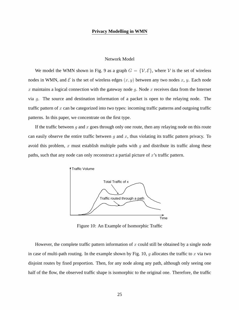
patterns. In this paper, we concentrate on the first type.

If the traffic betweeng andx goes through only one route, then any relaying node on this route

can easily observe the entire traffic betweeng andx, thus violating its traffic pattern privacy. To

avoid this problem,x must establish multiple paths withg and distribute its traffic along these

paths, such that any node can only reconstruct a partial picture ofx’s traffic pattern.

Time

Traffic Volume

Total Traffic of x

Traffic routed through a path

Figure 10: An Example of Isomorphic Traffic

However, the complete traffic pattern information ofx could still be obtained by a single node

in case of multi-path routing. In the example shown by Fig. 10, g allocates the traffic tox via two

disjoint routes by fixed proportion. Then, for any node alongany path, although only seeing one

half of the flow, the observed traffic shape is isomorphic to the original one. Therefore, the traffic

25

to x must be distributed along multiple route in a time-variant fashion, such that the traffic pattern

observed at any node is statistically different from the original pattern.

Traffic Entropy

We propose to use information entropy as a metric to quantifythe performance of a solution at

preserving the traffic pattern confidentiality. In what follows, we consider two nodesx andy. x is

the destination node of the traffic from the gatewayg to x. y is the observing node, which relays

packets tox and also tries to analyze the traffic ofx.

Time

Traffic Volume

……

Total Traffic of x

Figure 11: Sampling-based Traffic Analysis

Table 1: Notations used in Sec. III

V wireless node setE edge setg gateway nodex destination nodey observing nodeX random variable describingx’s traffic patternY X random variable describingx’s traffic pattern observed byyH(X) entropy ofXH(Y X) entropy ofY X

I(Y X , X) mutual information betweenX andY X

26

Basic Definition

Ideally, we view the traffic ofx as a continuous function of time, as shown in Fig. 11. In

practice, the traffic analysis is conducted by dividing timeinto equal-sized sampling periods, then

measuring the amount of traffic in each period, usually in terms of number of packets, assuming

the packet sizes are all equal. Therefore, as the first step, we discretize the continuous traffic curve

into a piece-wise approximation of discrete values, each denoting the number of packets destined

to x in a sampling period.

Now, we useX as the random variable of this discrete value.Y X is the random variable

representing the number of packets destined tox observed at nodey in a sampling period. We

denoteP (X = i) as the probability that the random variableX is equal toi (i ∈ N ) (i.e., the

probability that nodex receivesi packets in a sampling period). Likewise,P (Y X = j) is the

probability thatY X is equal toj (j ∈ N ), i.e., j packets destined tox go through nodey in a

sampling period.

Then the discrete Shannon entropy of the discrete random variableX is

H(X) = −∑

i

P (X = i) log2 P (X = i) (4)

H(X) is a measurement of the uncertainty about outcome ofX. In other words, it measures the

information of nodex’s traffic (i.e., the number of bits required to code the values ofX). H(X)

takes its maximum value when the value ofX is uniformly distributed. On the other hand, if

the traffic pattern is CBR (constant bit rate), thenH(X) = 0 since the number of packets at any

sampling period is fixed2. Similarly, we have the entropy forY X as follows.

H(Y X) = −∑

j

P (Y X = j) log2 P (Y X = j) (5)

2This offers the information-theoretic interpretation fortraffic padding: by flattening the traffic curve with blankpackets, the entropy of observable traffic is reduced to 0, which perfectly hides the information of the original trafficpattern.

27

Mutual Information

We define the conditional entropy of random variableX with respect toY X as

H(X|Y X) = −∑

j

P (Y X = j)∑

i

pij log2 pij (6)

wherepij = P (X = i|Y X = j) is the probability thatX = i given condition thatY X = j.

H(X|Y X) can be thought of as the uncertainty remaining aboutX afterY X is known. The joint

entropy ofX andY X can be shown as

H(X,Y X) = H(Y X) + H(X|Y X) (7)

Finally, we define the mutual information betweenX andY X as

I(Y X , X) = H(X) + H(Y X)−H(X,Y X)

= H(X)−H(X|Y X) (8)

which represents the information we gain aboutX from Y X .

Returning to the example in Fig. 10, let us assume that the observing nodey is located on one

route destined tox. Since the traffic shape observed aty is the same asx, at any sampling period,

if Y X = j, thenX must be equal to a fixed valuei, makingP (X = i|Y X = j) = 1. According

to Eq. (6), this makes the conditional entropyH(X|Y X) = 0. According to Eq. (8), we have

I(Y X , X) = H(X), implying that fromY X , we gain the complete information aboutX.

On the contrary, ifY X is independent fromX, then the conditional probabilityP (X = i|Y X =

j) = P (X = i), which maximizes the conditional entropyH(X|Y X) to H(X). According to

Eq. (8), we haveI(Y X , X) = 0,3 (i.e., we gain no information aboutX from Y X).

3By the definition of mutual information,I(Y X ,X) ≥ 0, with equality if and only ifX andY are independent.

28

In reality, sinceY X records the number of a subset of packets destined to nodex, it can not

be totally independent from the random variableX. Therefore, the mutual information should be

valued between the two extremes discussed above (i.e., 0 < I(Y X , X) < H(X)). This means that

nodey can still obtain partial information ofX ’s traffic pattern. However, a good routing solution

should minimize such mutual information as much as possiblefor any potential observing node.

More formally, we should minimize

maxY ∈V−X

I(Y X , X) (9)

the maximum mutual information that any node can obtain about X.

Penalty-based Routing Algorithm

In this section, we propose a penalty-based routing algorithm to achieve our goal of hiding traf-

fic patterns by exploiting the richness of available paths between two nodes in WMN. Specifically,

we choose to adopt thesource routingscheme. Such a choice is enabled by the fact that one node

can easily acquire the topology of the WMN it belongs to, whichis mid-sized (within 100 nodes)

and static.

When designing the algorithm, we also keep in mind the need to compromise between suffi-

cient security assurance and acceptable system overhead. We show in our algorithm that system

performance is satisfactory and security assurance is adequate. Shown in Tab. 2, the algorithm

operates in three phases,path pool generation, candidate path selectionand individual packet

routing. The notations used in Sec. III are listed in Tab. 3.

First, in the path pool generation phase, we generate a largeset of diversified routing paths

connecting the gatewayg and the destination nodex, denoted asSpaths. The path generation algo-

rithm is an iterative process of applying PBSP (Penalty-BasedShortest Path), a modified version

of Dijkstra’s algorithm. The PBSP algorithm is shown in the first part of Tab. 2. Here, each node is

assigned a penalty weight, and the weight of an edge is definedas the weighted average of penalty

weights of its two end nodes. The weight (or cost) of a path is defined as the sum of penalty weights

29

of all edges constituting this path. The algorithm runs in iterations. Initially, we set the penalty

weight of each node as 1, then run the Dijkstra’s algorithm tofind the first shortest path from the

gatewayg to x. Next, we increase the penalty weight for each node on this found path. This will

make these appeared nodes less competitive to other nodes inbecoming components of the next

path. After this, the algorithm proceeds to the next iteration, generating the second path, and all

nodes appearing on the second path are penalized through increasing their weights. This process

iterates until a sufficient number of paths are found. Second, in the candidate path selection phase,

we try to choose a combination of diversified routing paths, asubset of paths from the setSpaths ,

denoted asSselected. The paths inSselected are selected randomly fromSpaths. After each choice of

a path is placed intoSselected, the probability factor of that path is decreased to lower the chance

of multiple identical paths existing inSselected. Sselected is changed and renewed corresponding to

network activities. Third, in the packet routing phase, we choose randomly fromSselected one path

for each packet and increase the counter for the selected path subsetSselected. This Sselected path

subset expires after a counter reaches its predetermined threshold. ThenSselected is renewed by

calling the second phase again.

Since packets are assigned a randomly chosen path, and all these candidate paths are designed

to be disjoint, the chance that packets are routed in similarpaths is small. Our experimental results

confirm this intuition. This algorithm is designed to balance the needs of routing performance

(finding paths with smallest hop count) and preserving traffic pattern privacy (finding disjoint

paths). The penalty weight update function serves as the tuning knob to maneuver the algorithm

between these two contradictory goals. During the initialization, when the penalties of all nodes

are equal, the path found by the algorithm is indeed the shortest in terms of hop count. As a node

is chosen by more routes, its penalty weight monotonically increases, making it less likely to be

chosen again. Thus, as the algorithm proceeds, the newly-chosen paths (shortest in terms of its

aggregate penalty weight) become more disjoint from existing paths, but longer in terms of hop

count. The pace of such shift from “smallest hop-count path”to “disjoint path” is controlled by

30

how fast the penalty weight update function grows. Our experimental results confirm this rea-

soning. Finally, by randomly assigning packets along different paths, the algorithm maximally

disturbs the traffic pattern of anyg − x pair.

Although penalty-based routing has been used in existing literature [12], we are using it for

different objects. Their links were penalized for losses ormalicious behavior while our approach

applies it to avoid using links repeatedly to get better pathdiversity.

Experimental Results

Simulation Setup

We base our simulations on a randomly generated topology (Fig. 12) (600 x 600) with 30

nodes. The effective distance between two nodes is set to be 250. The whole process of simulation

consists of 400,000 logical ticks. In each single tick, a packet is generated at gateway node 0 and

its destination is randomly decided to be one of the other 29 nodes. To better simulate real network

traffic, we set the probability of 0.05 that at one tick no packet is generated (i.e., idle probability).

The distance delay factor is chosen to be 0.003 tick and the hop delay factor is decided as 0.05 tick.

We approximate hop delay at any node by multiplying the hop delay factor with its usage count by

all paths chosen initially.

With a relatively small node set, we choose 50 as ourPathPoolSize and 5 asSelPathNum.

The selected path subsetSselected for any destination node is renewed after sending 50 packets

to that node. To obtain multiple diversified paths with Dijkstra’s algorithm more quickly, we

introduce an exponential penalty function ontag of one node and usedγ as the parameter of an

exponential function when deciding on which edge to includein a candidate path. To slow down

the growing rate of exponential penalty function, we multiply the exponential function with a factor

α when calculatingEdgePenalty. To avoid getting too many identically paths in the beginning

stages, we amplify the influence of another node by multiplying tag of another node withβ. The

penalty parametersα, β, γ are chosen to be 0.5, 15, and 1.85, respectively.

31

Table 2: Penalty-based Routing Algorithm

/*Penalty-Based Shortest Path*/PBSP (Snode, Dnode)

For each nodev ∈ Vd[v]←∞prev[v]←∞visited[v]← 0

d[SNode]← 0Repeat

Get unvisited vertexv with the leastd[v]If d[v] ≥ ∞, Then v unreachableElsevisited[v]← 1For all v’s neighborsw

EdgePenalty = α[pow(γ, (w.tag))] + β(v.tag)If d[w] > d[v] + EdgePenalty

d[w]← d[v] + EdgePenalty

prev[w]← v

Until visited[v] = 1, ∀v ∈ V

/*GenerateSpaths for eachg − x pair*/GenPath()

For all non-gateway nodesxFor each nodev ∈ V

v.tag ← 1Repeat

PBSP(g, x)Get newg − x pathPnew from vectorprev[]StorePnew in Spaths

For all nodesv onPnew

v.tag ← v.tag + 1Until PathPoolSizepaths found.

/*SelectSselected for eachg − x pair*/SelPath()

Repeatrnd = rand() mod PathPoolSize

selectrndth path fromSpaths

Until SelPathNum paths selected

/*Decide path for arriving packet*/RoutePkt(Snode, Dnode)

Packets[Dnode]← Packets[Dnode] + 1rndpath = rand() mod SelPathNum

route packet along therndpathth path fromSselected

If Packets[Dnode] > ReSelPathCnt

Packets[Dnode]← 0SelPath()

32

Table 3: Notations used in Sec. III

v, w nodev.tag number of timesv is included by a pathα factor to slow down penalty rateβ factor to avoid many identical paths in the beginning stagesof path gen-

erationγ base of exponential penalty functiond[] penalty vector for every nodeprev[] vector to storePnew in reverse orderPackets[] vector to store the number of arrived packets for every node

0

100

200

300

400

500

600

0 100 200 300 400 500 600

Y P

ositi

on

X Position

0

1

2

3

4

5

6

7

8

9

10

11

12

13

14

15

16

17

18

19

2021

22

23

24

25

26

27

28

29

Gateway

Figure 12: Experimental Topology

33

Traffic Entropy and Mutual Information

The total 400,000 ticks are divided into 20 periods. Each period is then divided into 50 intervals

and one interval is 400 ticks long. Within each interval, foreach destination nodex, we count the

number of packets that all other nodesy have relayed forx. Then for each period, we independently

calculate the traffic entropiesH(X), H(Y X), and mutual informationI(Y X , X) based on their

definitions in Sec. III.

0.5

1

1.5

2

2.5

3

3.5

4

0 2 4 6 8 10 12 14 16 18 20

Tra

ffic

Info

rmat

ion

Ent

ropy

Number of Periods

H(23-1)H(1-1)

MI(23-1,1-1)

0.5

1

1.5

2

2.5

3

3.5

4

0 2 4 6 8 10 12 14 16 18 20

Tra

ffic

Info

rmat

ion

Ent

ropy

Number of Periods

H(9-16)H(16-16)

MI(9-16,16-16)

(a) Destination: Node 1, Observer: Node 23 (b) Destination: Node 16, Observer: Node 9

Figure 13: Traffic Entropy along Time (Single Observer,γ = 1.85)

Due to the space limit, we only show part of our results. Amongall nodes in the network,

we choose two sets of nodes. Nodes in the first set{1, 6, 11, 15, 23, 24, 25, 29} are close to (2 to

3 hops) the gateway node 0. Nodes in the second set{2, 3, 7, 16, 17, 28} are at the edge of the

network, 4 to 5 hops away from the gateway. We choose two representative nodes, 1 and 16, out

of each set.

Fig. 13 shows the variance of traffic entropy and mutual information as a function of the time.

In Fig. 13 (a),H(1−1) denotes the traffic entropy of node1. H(23−1) denotes the traffic entropy

of node 23 based on its observation on node 1.MI(23− 1, 1− 1) denotes the mutual information

that node 23 shares with node 1. The same notation rules applyfor Fig. 13 (b), where node 16 is

the destination, and 9 is the observer. In both pictures, theobserving node only shares40% or less

of the total information about the observed destination node at any sampling period.

34

0

0.5

1

1.5

2

2.5

3

3.5

4

0 2 4 6 8 10 12 14 16 18 20

Tra

ffic

Info

rmat

ion

Ent

ropy

Number of Periods

H(1-1)MI(29-1,1-1)

MI(4-1,1-1)MI(26-1,1-1)

MI(7-1,1-1)

0

0.5

1

1.5

2

2.5

3

3.5

4

0 2 4 6 8 10 12 14 16 18 20

Tra

ffic

Info

rmat

ion

Ent

ropy

Number of Periods

H(16-16)MI(26-16,16-16)

MI(2-16,16-16)MI(1-16,16-16)

MI(10-16,16-16)

(a) Destination: 1, Observers: Node 4, 7, 26, 29 (b) Destination: 16, Observers: Node 1, 2, 10, 26

Figure 14: Traffic Entropy in Different Sampling Periods (Multiple Observers,γ = 1.85)

This observation is further confirmed in Fig. 14, where we plot the time-variant mutual infor-

mation that destinations 1 and 16 share with other randomly-chosen observing nodes. These results

show that with our algorithm, the destination node is able toconsistently limit the proportion of

mutual information it shares with the observing nodes.

Which Nodes have more Mutual Information?

In Fig. 15 (a), we calculate the time-averaged mutual information for all observing nodes with

respect to the destination node 1. (The nodes are sorted in ascending order.) Here, we observe an

almost linearly-growing curve except at its head and tail. For nodes at the head of the cure, their

mutual information is 0 since they lie at the outer rim of the network. Hence, they are not chosen

by our routing algorithm to relay traffic for node 1. At the tail of the curve is destination node 1,

whose mutual information is actually the traffic entropy of its own. In Fig. 15 (b), we observe the

same phenomenon for destination 16, except at the head of thecurve. This is because its network

location is opposite to the gateway, making every node of thenetwork to be its candidate relaying

node.

This leads us to investigate whether such distribution of mutual information is related with

other factors. We considered the mutual information of eachnode with certain metrics, such as its

distance to the destination. However, we failed to find any causal relationship. We also considered

sorting the observation nodes based on their averaged relayed traffic (i.e., the average number

35

0

0.5

1

1.5

2

2.5

3

3.5

4

0 5 10 15 20 25 30

Traf

fic In

form

atio

n E

ntro

py

Node

3 7 16 17 27 28 10 2 9 22 26 8 29 25 5 15 11 24 4 13

20 21 6 14 12 23 18 19

1 Average Mutual Information

0

0.5

1

1.5

2

2.5

3

3.5

4

0 5 10 15 20 25 30

Traf

fic In

form

atio

n E

ntro

py

Node

15 13 10 7 11 1

29 20 22 24 8 21 25 27 5 17 3 28 18 14 19 12 23 9 2 26 4 6

16 Average Mutual Information

(a) Destination: Node 1 (γ = 1.85) (b) Destination: Node 16 (γ = 1.85)

Figure 15: Sorted Traffic Mutual Information

of packets that each node relays in a sampling period) on a log-log scale. We found a linear

distribution as shown in Fig. 16.

1

0.1 1 10

Traf

fic In

form

atio

n E

ntro

py

Average Relayed Traffic

0

2

4

6

8

10

12 14

18

20

22

24

26

Average Mutual Information

1

0.1 1 10

Traf

fic In

form

atio

n E

ntro

py

Average Relayed Traffic

0

2 4 6

8

10

12 14

16

18

20 22

24

26

28

Average Mutual Information

(a) Destination: Node 1 (γ = 1.85) (b) Destination: Node 16 (γ = 1.85)

Figure 16: Power-law Correlation of Mutual Information and Amount of Traffic Relayed

Obviously, such a power-law correlation tells us that the more traffic an observing node relays

for a destination node, the more mutual information can be obtained about its traffic entropy.

Furthermore, it gives us one way to experimentally quantifythe relationship of these two metrics.

Let T be the amount of traffic relayed andI be the mutual information, then their power-law

relationship can be written as

I = aT k (10)

wherea is the constant of proportionality andk is the exponent of the power law, both of which can

be measured from Fig. 16. Ifk < 1, then the mutual information of an observing node grows in a

sub-linear fashion to the amount of its relayed traffic increases. Ifk ≥ 1, this mutual information

36

grows in a super-linear fashion. From Fig. 16 and the same results for other destination nodes, we

havek < 1. This implies that an observing node has to relay more and more traffic each time, in

order to make its mutual information further grow with the same increment.

Trade-off between Performance Degradation and Traffic Privacy

Finally, we study the performance trade-off of our algorithm by tuning its exponential penalty

function baseγ. The performance degradation introduced by our algorithm is captured by the

average hop ratio. For each gateway-destination pairg − x, this metric is defined as the ratio

between the average number of hops a packet goes through using our algorithm and the number

of hops of the shortest path betweeng ands. From Fig. 17, we can see that the average hop ratio

increases asγ increases. The direct neighbors of the gateway are less sensitive to the change ofγ.

(See node 6 in Fig. 17(a) and node 23 in Fig. 17(b).)

0.95

1

1.05

1.1

1.15

1.2

1.25

1.3

1.35

1.4

1.45

1.5

1.12 1.31 1.57 1.85 2.06 2.59

Rat

ios

Parameter γ

Node 1 Node 6

Node 11 Node 15 Node 17 Node 24 Node 29

0.95

1

1.05

1.1

1.15

1.2

1.25

1.3

1.35

1.4

1.45

1.5

1.12 1.31 1.57 1.85 2.06 2.59

Rat

ios

Parameter γ

Node 2 Node 3 Node 7

Node 16 Node 23 Node 25 Node 28

(a) Hop Ratio of Nodes in the First Set (b) Hop Ratio of Nodes in the Secondset

Figure 17: Average Hop Ratio

In Fig. 18 and Fig. 19 we find that, under shortest path routing, the mutual information of a

node is 0 if it is not on the path to the destination node. Otherwise, the mutual information of a

node is much higher than when using the new algorithm. Also worth noting is the observation

that increasingγ has different impact on different nodes, depending on its distance to gateway,

destination, and its location in the WMN. Consider node 12 (Fig. 18) and 6 (Fig. 19). Since they

lie near the gateway node and are relatively centrally situated, their observed mutual information

varies little with respect to changes ofγ. In contrast, for node 22 (Fig. 18), which is far away

37

from destination node 1 and on edge of WMN. The mutual information shared between itself and

node 1 increases with the growth ofγ, indicating more traffic is routed through farther nodes. This

tendency of routing packets via farther nodes leads to a higher average number of hops, which is

confirmed by our analysis of the average hop ratio.

0.5

1

1.5

2

2.5

3

3.5

4

0 2 4 6 8 10 12 14 16 18 20

Tra

ffic

Ent

ropy

Number of Periods

ShortestPath1.121.571.852.59

0

0.2

0.4

0.6

0.8

1

1.2

0 2 4 6 8 10 12 14 16 18 20

Tra

ffic

Ent

ropy

Number of Periods


(a) Observer: Node 12 (b) Observer: Node 15

0

0.1

0.2

0.3

0.4

0.5

0.6

0.7

0.8

0.9

0 2 4 6 8 10 12 14 16 18 20

Tra

ffic

Ent

ropy

Number of Periods


0

0.2

0.4

0.6

0.8

1

1.2

0 2 4 6 8 10 12 14 16 18 20

Tra

ffic

Ent

ropy

Number of Periods


(c) Observer: Node 22 (d) Observer: Node 26

Figure 18: Traffic Mutual Information under Different Penalty Parameters (Destination: Node 1)

However, traffic mutual information tends to decrease onceγ gets too high (2.59 in Fig. 18).

This is due to the fact that when penalty values of many possible edges get large quickly, their

relative differences become less. Consequently, the numberof candidate paths decreases. The

fluctuation of node 26 (Fig. 18) is due to its position in center of the topology and being equi-

distance between the gateway and destination nodes. Similar observations can be made about the

mutual information values of destination node 16 (Fig. 19).

We observe from Fig. 20 that the algorithm achieves our goal of preserving traffic patterns. It

is easy to conclude that in normal shortest path routing, allrelaying nodes share the same traffic

information with the destination node, as shown by the tail of the ShortestPathcurve in Fig. 20.

38

0.5

1

1.5

2

2.5

3

3.5

4

0 2 4 6 8 10 12 14 16 18 20

Tra

ffic

Ent

ropy

Number of Periods


0

0.2

0.4

0.6

0.8

1

1.2

1.4

1.6

1.8

0 2 4 6 8 10 12 14 16 18 20

Tra

ffic

Ent

ropy

Number of Periods


(a) Observer: Node 6 (b) Observer: Node 2

0

0.2

0.4

0.6

0.8

1

1.2

1.4

1.6

1.8

0 2 4 6 8 10 12 14 16 18 20

Tra

ffic

Ent

ropy

Number of Periods


0

0.2

0.4

0.6

0.8

1

1.2

1.4

1.6

1.8

0 2 4 6 8 10 12 14 16 18 20T

raffi

c E

ntro

py

Number of Periods


(c) Observer: Node 14 (d) Observer: Node 19

Figure 19: Traffic Mutual Information under Different Penalty Parameters (Destination: Node 16)

However, for our algorithm, the mutual information shared between relaying nodes and the desti-

nation node varies less among the relaying nodes. Asγ increases, the more leveled off the curve

becomes, and the closer we are to the goal of minimizing the greatest mutual information, as for-

mulated in Eq. 9. It is also interesting to observe that the mutual information is 0 for some nodes far

away from both the gateway and the destination nodes, e.g., Fig. 20 (a), when destination is 1. In

contrast, all nodes participate in relaying packets for destination 16 (Fig. 20 (b)), since destination

and gateway nodes are in opposite directions with respect toWMN topology.

Collusion Analysis

The relative small size of a typical WMN makes it easy for spatially close eavesdroppers to

find each other. This is concerning since there is a higher possibility of collusion of two malicious

observers by exchanging their observed traffic patterns. This motivates us to make our proposed

39

0

0.5

1

1.5

2

2.5

3

3.5

4

0 5 10 15 20 25 30

Tra

ffic

Ent

ropy

Node


0

0.5

1

1.5

2

2.5

3

3.5

4

0 5 10 15 20 25 30

Tra

ffic

Ent

ropy

Node


(a) Destination: Node 1 (b) Destination: Node 16

Figure 20: Sorted Traffic Mutual Information under Different Penalty Parameters

solution resilient to such collusion threats. To analyze the extent to which collusion reveals infor-

mation about the original traffic pattern, we study the fluctuation of the observed traffic informa-

tion. In this way, we can analyze how much additional information the colluders can collect about

the original traffic.

Problem Description

In the first part of this chapter we focused on traffic confidentiality. We studied the problem

of traffic pattern concealment via routing control. However, the relative small size of a WMN,

aided by the stationary adjacent routers, invites a higher possibility of collusion between several

observing relaying routers in the network. Since it is highly possible that different observers will

know about various “ups and downs” of target’s traffic, if malicious observers interchange their

observed traffic information of target users, the combined observations could reveal significant

information about the original traffic pattern. This is illustrated in Fig. 21. Given the size of

the network (e.g., less than 100 neighbor nodes), we think itis more common that less than two

malicious observers exist simultaneously. Hence we focus on analyzing the collusion problem of

two observers in this work.

The parameters that affect significantly our collusion analysis include the choice of cooperating

observers and the destination target node. Since any routing algorithm will largely depend on the

topology of the network and the relative positions of the observers, the source and destination

40

Figure 21: Collusion Reveals Significant Portion of Original Traffic Pattern.

nodes can affect portions of the revealed traffic pattern greatly. Another important parameter is the

base of the exponential penalty function explained in Sec. III.

Colluded Traffic Mutual Information

Our modeling of colluded traffic analysis tries to study the influence of collusion to observed

traffic patterns of every period. This can help us to evaluatethe resilience of our proposed PBSP

routing algorithm against collusion attack. In what follows, we consider three nodesx, y, andz.

x is the destination node of the traffic from the gatewayg to x. Nodesy andz are the observing

nodes, which relay packets forx, and also try to analyze the traffic ofx. Due to the uncertainty of

routing,y andz may or may not be on the same path over time.

Initially, we identify a metric to capture colluded observations. Based on definition of traffic

mutual information defined in Sec. III, we measure the colluded observation about destinationx

with mutual information betweenx and(y, z). The traffic observations byy andz together can

be deemed as a joint distribution of variableY X andZX . The colluded traffic mutual information

I(Y X , ZX ; X) of random variable(Y X , ZX) with respect toX can then be defined as

I(Y X , ZX ; X) = H(Y X , ZX) + H(X)−H(Y X , ZX , X) (11)

whereH(Y X , ZX , X) is the joint entropy ofY X , ZX , andX. I(Y X , ZX ; X) represents the

information gained aboutX from (Y X , ZX) (i.e., fromy andz acting together). Their relationship

is shown in Fig. 22.

41

Table 4: Notations used in Sec. III.

V wireless node setE edge setg gateway nodex destination nodey, z observing nodesX random variable describingx’s traffic patternY X , ZX random variables describingx’s traffic pattern observed byy

andz, separately(Y X , ZX) random variable describingx’s traffic pattern observed byy

andz togetherH(X) entropy ofXH(Y X) entropy ofY X

H(Y X , ZX , X) joint entropy ofY X , ZX , andXI(Y X ; X) mutual information betweenX andY X

I(Y X , ZX ; X) colluded mutual information betweenX and(Y X , ZX)

Figure 22:I(Y X , ZX ; X), H(Y X , ZX) andH(Y X , ZX , X) in Venn Diagram.

42

Simulation Results

For ease of notation in the following discussion, we useH(Y,X) to denoteH(Y X , X) (i.e.,

the entropy of traffic thaty observes aboutx). Similarly, we simplify the joint traffic entropy

H(Y X , ZX) asH(y, z, x), whereY X , ZX denote the portions of traffic thatY andZ observe about

X. In a subtly different way, we denoteI(Y X ; X) asI(Y ; X) andI(Y X , ZX ; X) asI(Y, Z; X).

Traffic Curves

We first present the measured traffic curves as a function of time. In Fig. 23, node 1 is the

destination node. We easily conclude that its traffic (i.e.,node 1 observing itself) is always the

largest. This is because any node can observe the complete traffic of itself while other nodes can

only observe a portion of it.

0

5

10

15

20

25

0 50 100 150 200 250

Traf

fic

Interval

Traffic(1)Traffic(15:1)Traffic(28:1)

Traffic(15,28:1)

Figure 23: Sampled Traffic Curves from Experiment.

Another observation is the fact that the colluded knowledgeabout traffic activity of node 1 (in

squares), as expected, is higher than any single observer, either node 15 or node 28. Moreover, we

confirm that, although, generally speaking, node 15 observes much more traffic of node 1, during

some intervals, node 28 out-performs node 15, which increases the aggregated knowledge about

node 1’s total traffic activity. Example intervals are thosenear interval 100 and 150.

43

Colluded Traffic Mutual Information: Single Pair of Observer s

The next results are the comparisons of colluded traffic mutual information (I(y, z; x)), single

observer mutual information (I(y; x) andI(z; x)), original traffic entropy (H(x)), separately ob-

served traffic entropy (H(y, x) andH(z, x)) and joint entropy (H(y, z, x)).4 From our analysis in

Sec. III, we conclude the following relationships among these values:

1. H(y, x), H(z, x) ≤ H(y, z, x) ≤ H(x);

2. I(y, x), I(z, x) ≤ I(y, z, x) ≤ H(x);

3. I(y, x) ≤ H(y, x) ≤ H(x);

4. I(z, x) ≤ H(z, x) ≤ H(x);

We can verify that the simulation results shown in Fig. 24 satisfy these relationships. This

means our modeling of traffic activity not only characterizes the traffic pattern fluctuation across

the time, but it also actually illustrates the collusion problem. The simulation results of our model

conforms to our conjectures.

The overlapping curves in Fig. 24(b) indicates that node 23 does not observe any traffic of node

1. This is true since nodes 23 and 1 are on opposite sides of thenetwork. Fig. 25 shows similar

results, where node 16 is the destination.

Colluded Traffic Mutual Information: Multiple Pairs of Observ ers

The simulation results confirm the necessary relationshipslisted previously. We now analyze

how collusion affects the performance of Penalty-based Shortest Path (PBSP) routing. To accom-

plish this, we study the colluded traffic mutual informationof several pairs of observers. In this

way, we compare the ratio of traffic information collected bydifferent pairs of observers.

From Fig. 26 we observe that the conditions listed above still hold. Additionally, based on the

average values of the colluded traffic mutual information curves in both figures, we infer that the

4Please note thatH(y, z, x), according to our notation, meansH(Y X , ZX).

44

0

0.5

1

1.5

2

2.5

3

3.5

4

0 0.5 1 1.5 2 2.5 3 3.5 4

Tra

ffic

Ent

ropy

Period

H(1)H(6,1)

H(28,1)H(6,28,1)

I(6;1)I(28;1)

I(6,28;1)

0

0.5

1

1.5

2

2.5

3

3.5

4

0 0.5 1 1.5 2 2.5 3 3.5 4

Tra

ffic

Ent

ropy

Period

H(1)H(23,1)H(28,1)

H(23,28,1)I(23;1)I(28;1)

I(23,28;1)

(a) single pair of observers: 6, 28 (b) single pair of observers: 23,28

0

0.5

1

1.5

2

2.5

3

3.5

4

0 0.5 1 1.5 2 2.5 3 3.5 4

Tra

ffic

Ent

ropy

Period

H(1)H(21,1)H(29,1)

H(21,29,1)I(21;1)I(29;1)

I(21,29;1)

0

0.5

1

1.5

2

2.5

3

3.5

4

0 0.5 1 1.5 2 2.5 3 3.5 4

Tra

ffic

Ent

ropy

Period

H(1)H(15,1)

H(4,1)H(15,4,1)

I(15;1)I(4;1)

I(15,4;1)

(c) single pair of observers: 21, 29 (d) single pair of observers: 15, 4

Figure 24: Colluded Traffic Mutual Information (Destination: 1, γ = 1.85).

0

0.5

1

1.5

2

2.5

3

3.5

4

0 0.5 1 1.5 2 2.5 3 3.5 4

Tra

ffic

Ent

ropy

Period

H(16)H(6,16)

H(28,16)H(6,28,16)

I(6;16)I(28;16)

I(6,28;16)

0

0.5

1

1.5

2

2.5

3

3.5

4

0 0.5 1 1.5 2 2.5 3 3.5 4

Tra

ffic

Ent

ropy

Period

H(16)H(23,16)H(28,16)

H(23,28,16)I(23;16)I(28;16)

I(23,28;16)

(a) single pair of observers: 6, 28 (b) single pair of observers: 23,28

0

0.5

1

1.5

2

2.5

3

3.5

4

0 0.5 1 1.5 2 2.5 3 3.5 4

Tra

ffic

Ent

ropy

Period

H(16)H(21,16)H(29,16)

H(21,29,16)I(21;16)I(29;16)

I(21,29;16)

0

0.5

1

1.5

2

2.5

3

3.5

4

0 0.5 1 1.5 2 2.5 3 3.5 4

Tra

ffic

Ent

ropy

Period

H(16)H(15,16)

H(4,16)H(15,4,16)

I(15;16)I(4;16)

I(15,4;16)

(c) single pair of observers: 21, 29 (d) single pair of observers: 15, 4

Figure 25: Colluded Traffic Mutual Information (Destination: 16,γ = 1.85).

45

0

0.5

1

1.5

2

2.5

3

3.5

4

0 0.5 1 1.5 2 2.5 3 3.5 4

Tra

ffic

Ent

ropy

Period

H(1)I(21;1)

I(6;1)I(28;1)

I(21,6;1)I(21,28;1)

I(6,28;1)

0

0.5

1

1.5

2

2.5

3

3.5

4

0 0.5 1 1.5 2 2.5 3 3.5 4

Tra

ffic

Ent

ropy

Period

H(16)I(21;16)

I(6;16)I(28;16)

I(21,6;16)I(21,28;16)

I(6,28;16)

(a) destination: 1, observers: 21, 6, 28 (b) destination: 16, observers: 21, 6, 28

Figure 26: Colluded Traffic Mutual Information (Multiple Pairs of Observers,γ = 1.85).

PBSP algorithm works well when there are two observers colluding to share their knowledge about

one destination.

0

0.5

1

1.5

2

2.5

3

3.5

4

0 0.5 1 1.5 2 2.5 3 3.5 4

Tra

ffic

Ent

ropy

Period

H(1)I(15;1)

I(6;1)I(4;1)

I(15,6;1)I(15,4;1)

I(6,4;1)

0

0.5

1

1.5

2

2.5

3

3.5

4

0 0.5 1 1.5 2 2.5 3 3.5 4

Tra

ffic

Ent

ropy

Period

H(16)I(15;16)

I(6;16)I(4;16)

I(15,6;16)I(15,4;16)

I(6,4;16)



To further confirm this conjecture, we examine another set ofsimulation results, as shown in

Fig. 27. The colluded traffic mutual information of all observer pairs in this figure does not exceed

half of the total traffic information. In Fig. 27(b), however, we notice some small error in the curves

(i.e., the value ofI(15, 6; 16) is slightly less than that ofI(15; 16) for period 2). Although this is

a small error, it is similar to approximation error when computing H(Y X , ZX , X). Instead of

employing three parallelPacketCounters to get the aggregate traffic information, the simulation

program approximates it, based on the packet count value dictionary, which results in a lower

I(Y X , ZX ; X) value.

46

The same explanation applies to the discrepancy in Fig. 28(a). The average value of colluded

traffic mutual information of all observer pairs in Fig. 28 remains approximately less than half of

the total traffic entropy of the target node across all time periods.

0

0.5

1

1.5

2

2.5

3

3.5

4

0 0.5 1 1.5 2 2.5 3 3.5 4

Tra

ffic

Ent

ropy

Period

H(1)I(21;1)I(15;1)

I(7;1)I(21,15;1)

I(21,7;1)I(15,7;1)

0

0.5

1

1.5

2

2.5

3

3.5

4

0 0.5 1 1.5 2 2.5 3 3.5 4

Tra

ffic

Ent

ropy

Period

H(16)I(21;16)I(15;16)

I(7;16)I(21,15;16)

I(21,7;16)I(15,7;16)



Related Work

Multi-hop wireless mesh networks (WMN) are gaining popularity. Current deployments of

WMN either serve as substitutes for traditional WLAN Internetconnections, or aim at providing

infrastructural large-scale network access [45].

Existing research [6, 32, 14, 11] on WMN has focused on how to better utilize the wireless

channel resource and enhance its performance. For example,some researchers derive the optimal

node density following a capacity analysis [28], while others devise more efficient [18] protocols.

A survey paper by Akyildiz et al. [10] provides a good source for existing and ongoing research

about wireless mesh networks. Some of the proposed solutions include equipping mesh routers

with multiple radios and distributing the wireless backbone traffic over different wireless channels,

routing the traffic through different paths [22, 57], or a joint solution of these two [47, 46]. Theo-

retical studies show that these approaches can significantly increase the capacity of WMN [36, 34].

These results make significant steps towards enabling WMN as an attractive alternative for broad-

band Internet access.

47

Information Theory is widely used and proves to be a useful tool. It applies to situations

where variations are frequent and unpredictable. It also helps to identify patterns and the extent

of observed variations. Serjantov et al. [51] define an information theoretic anonymity metric and

suggest developing more sophisticated probabilistic anonymity metrics. Existing research in the

Internet setting employs information theoretical coding [33]. However, such analysis is often too

complex and impractical for WMNs. The book by David Mackay provides a good source for

background knowledge in information theory [40].

Privacy has been a major concern of Internet users [17, 55]. Two types of techniques have been

proposed to preserve user traffic privacy and increase the difficulty for performing harmful traffic

analysis [48, 13] in the existing literature of traffic pattern concealment. They are anonymous over-

lay routing [59, 13, 26, 33, 27, 21, 49] and traffic padding [52]. The former approach provides user

anonymity in an end-to-end connection through layered encryption and multi-hop overlay routing.

The latter one conceals the traffic shape by generating a continuous random data stream at the link

level. However neither approach is applicable to WMN directly. First, the number of nodes in

a WMN is limited. Second, the traffic forwarding relationshipamong nodes is strongly depen-

dent on their locations and the network topology. To better utilize the wireless channel resource

and enhance the data delivery performance, a shortest path routing technique is usually selected

(or a load-balanced routing scheme is employed). Such observations indicate that the anonymity

systems, which rely on relaying traffic among nodes (randomly selected out of thousands) to gain

anonymity, can not effectively preserve users’ privacy in WMN (or at the cost of significant per-

formance degradation). On the other hand, traffic padding mechanisms consume a considerable

amount of network bandwidth, which makes it impractical in resource-constrained WMNs.

The schemes designed for wireless ad-hoc networks [56, 15] are more focused on location and

identity privacy. While these are still issues in WMN, the traffic rates and temporal variations are

more meaningful and consequential. To the best of our knowledge, no existing work has studied

collusion problems about traffic privacy in the scenario of Wireless Mesh Networks.

48

Conclusion

This chapter identifies the problem of traffic privacy preservation in wireless mesh networks

(WMN). To address this problem, we introduced a light-weightarchitecture for WMN, then pro-

posed “traffic entropy”, an information theoretic metric toquantify how well a solution performs

at preserving traffic pattern confidentiality. A new penalty-based shortest path routing algorithm

was described and analyzed. We evaluated our scheme in the presence of two malicious colluding

nodes. Simulation results show that our algorithm is able topreserve traffic privacy, while min-

imizing the network performance degradation within acceptable ranges. Our simulation analysis

demonstrate the resilience of our solution against two colluding observers.

For future work, we will focus on the following problems. First, although our algorithm is

evaluated in a single-radio, single-channel WMN setting, itcan be easily enhanced to exploit the

advantages of multiple radios and multiple channels available in WMNs. Performance evaluation

of the enhanced algorithm in such settings should provide interesting results. It is also beneficial

to evaluate the possibility of devising a distributed routing algorithm that achieves the same goal

but which supports better scalability.

49

CHAPTER IV

PRIVACY PRESERVATION IN WIRELESS SENSOR NETWORKS

Preserving information confidentiality is a critical issuefor wireless sensor networks. While

existing security solutions (e.g., encryption) could protect the data content, they can not protect

against direction-based traffic analysis. Preserving directional traffic privacy is a challenging prob-

lem for wireless sensor networks, as the conventional approaches such as traffic padding and rout-

ing control are usually very resource-consuming. This chapter investigates the effectiveness of

privacy preserving mechanisms and seeks an optimal solution for preserving privacy in a resource-

constrained environment. It presents a novel privacy modelthat characterizes the application-

specific impact of pattern revelation. Via this privacy model, the privacy preservation problem

is formulated as an optimization-problem, where optimal routing schemes are derived. Through

theoretical analysis and simulation validation, we evaluate the performance of the optimal pri-

vacy preservation routing scheme and demonstrate its trade-off in privacy preservation and routing

efficiency.

Introduction

Wireless sensor networks are formed by a collection of sensor devices which are capable of

sensing, data processing, and communicating via wireless medium [29]. They can be readily

deployed in diverse environments to collect and process useful information in an autonomous

manner. Thus, they have a wide range of applications in the areas of health care, military, and

disaster detection. Sensor networks are envisioned to change the way people interact with the

physical environment and to have a significant social impact.

One of the most notable challenges that threaten successfuldeployment of sensor networks is

the protection of information privacy. The challenge comesfrom two characteristics of wireless

sensor networks: (1) open wireless medium prone to eavesdropping;and (2) sensors prone to phys-

ical capture, which make it vulnerable to a variety of attacks. For a sensor network that provides

50

surveillance service, information communicated within the sensor networks involves when and

where an event happens, and what is the event. This defines twotypes of information privacy –

the contextual privacy (when and where) and the content-wise privacy (what) [30]. It is obvious

that the content-wise privacy is a critical issue for sensornetworks. The contextual information,

however, also reveals important information with respect to the sensor network operation. In an

event-driven sensor network, where messages are only generated and sent upon the detection of

certain event, the attackers can easily infer the contextual information (location and time of the

event) by observing the traffic patterns.

Content-wise privacy is most often protected via message encryption. In the existing literature,

the security mechanisms that support the content-wise privacy has been extensively researched

(e.g., link-level security solution [31], key distribution [23]). Only limited work, however, has

been done on the contextual privacy issues associated with sensor communication. The work of

[30], one of the first works on contextual privacy, has studied protecting location information (so

called location privacy). In this work, the authors study a sensor network application scenario

of panda hunting. They define location privacy and provide a privacy preservation solution via

controlled random routing and flooding. Though the work of [30] provides a convincing solution

and makes an important step towards location privacy, two major issues in the area of contextual

privacy:

• Lack of a precise definition of contextual privacy which is generalizeable into different ap-

plication scenarios.

• Lack of an analytical model that balances resource requirements of privacy preservation

solutions and their effectiveness. Many of the contextual privacy preservation approaches,

such as traffic padding and routing control, are quite resource-consuming. For resource-

constrained sensor networks, it is important to carefully examine the resource requirements

of these solutions and provide a tuning mechanism can trade-off effectiveness against re-

source requirements.

51

To address the above issues, this chapter presents an optimization-based theoretical framework

that characterizes the effectiveness of privacy preserving mechanisms. Our definition of privacy is

general and can be customized to application-specific scenarios. We focus on the location privacy

issue in wireless sensor networks in this work.

The chapter seeks an optimal solution for preserving privacy in a resource-constrained environ-

ment. It presents a novel privacy model based on an attacker penalty function, which characterizes

the application-specific impact of pattern revelation. Viathis privacy model, the privacy preser-

vation problem is formulated as an optimization problem where the optimal routing schemes are

derived. Through theoretical analysis and simulation validation, we show several important prop-

erties of the optimal privacy preservation.

The remainder of this chapter is organized as follows. Sec. IV presents the attacker and privacy

models. These models are used further in Sec. IV to formulateprivacy preservation as an optimiza-

tion problem. Sec. IV.[TODO] The simulation results are provided in Sec. IV demonstrates how

an optimal routing protocol can be designed to have good trade-off between privacy preservation

and network performance. A review of the existing literature is provided in Sec. IV. We present

conclusions in Sec. IV.

Model

Sensor Network Model

We consider an event-driven sensor network with a set of sensor nodesn ∈ N as shown

in Fig. 29. The event setE = {e} denotes the set of all possible events in this network. In

this chapter, we focus on the events that are characterized by their geographical locations. For

example, in the dirty bomb detection and localization scenario [3], the static sensors are deployed

around a stadium to report position data about the moving node. LetE be the random variable

that represents the detected event in the sensor network. Then the probability that this event ise is

denoted asPr(E = e), or in abbreviationPr(e).

52

attackerEvent e

observation d

Figure 29: Example Sensor Network.

When an evente is detected in the sensor network, the sensors that detect the event will send

messages among themselves and/or to the data sink. We assumethat the confidentiality and in-

tegrity of the message content are protected via data encryption and message authentication code.

If source routing is used in the network, then the source route information carried in the packet

header is also protected.

Attacker Model

The attacker tries to infer the event occurred in the sensor network based on his observations.

Since the packets are encrypted, the attackers could only doso by observing the traffic patterns

(e.g., from which direction packets are coming). Depending on theobservation location(s) of the

attacker and his observation range, different observations may be made for a single event. Without

loss of generality, we assume that an attacker has a fixed set of observation locations and ranges

when observing a single event. Thus, for an evente, there is only one possible observationd for a

particular attacker. Let us denote the set of all possible observations from attackerA upon different

events asDA. We further denote the set of all possible observations fromdifferent attackers with

different locations and observation ranges asD =⋃

ADA.

Upon observingd ∈ DA, the attacker A may infer a set of possible eventsE = {e}, and take

some corresponding actions. For example, he may deduce thatthe dirty bomb needs to be moved

to a new position. If the real event that occurs ise, then we model the utility of the attacker by

inferring evente via anattacker pay-off functionS(e, e). A positive value ofS(e, e) indicates the

gain of the attacker when his inferred event is equal to (or close to) the true event; while a negative

53

value represents the penalty to the attacker if his inference is far away from the true event. Here

we give several examples to illustrate the concept of the pay-off functionS(e, e).

Example 1.

S(e, e) =

1 if e = e;

−1 otherwise.(12)

In this example, the attacker will get a pay-off value of1 if his inferred evente is the true evente.

Otherwise, the pay-off is−1, which reflects the penalty on him to react to the wrong events.

Example 2.S(e, e) = F (|le, le|) (13)

wherele and le are the locations of eventse ande, and|le, le| is the distance between these two

locations. In this example, the events are identified by their locations. The attacker’s pay-off

depends on the distance between the inferred evente and the true evente. The functionF (·) could

take different shapes which reflect different degrees of sensitivity of revealing the event location to

the attacker. See Fig. 30. In this figure, the convex curve represents that an attacker is sensitive to

event location revelation.

0 1 2 3 4 5 6 7 8-8

-6

-4

-2

0

2

4

6

8

Distance

Pen

alty

Concave

Linear

Convex

Figure 30: Example Penalty Functions of Different Sensitivity to Event Location Revelation.

54

When the true event ise, the total pay-offS for the attacker from inferring and reacting to event

setE is

S(e, E) =∑

e∈E

S(e, e) (14)

It is obvious that the optimal strategy of a rational attacker is to infer and react to the event setE

so that his total pay-off is maximized, implying:

maxE

∑

e∈E

S(e, e) (15)

Without knowing the true evente, the attacker determines his strategy by estimating his total

pay-off S based on his observationd. The estimation is done through the relation between an

event and the possible observations by the attacker. LetPr(e|d) be the probability of evente’s

occurrence ifd is observed. Then, the attacker’s pay-offS of inference setE based on observation

d is estimated as

S(d, e, E) =∑

e∈E

{Pr(e|d)×∑

e∈E

S(e, e)} (16)

Thus the attacker’s optimal strategy is to deriveE so thatS is maximized. To do that, he first

needs to estimatePr(e|d). Note that some events in the sensor network may not be observable by

attackerA, depending on his observation location and range. We denotethe set of events that could

be observed byA asEA. Obviously,∀e /∈ EA, P r(e|d) = 0. For an event observable by attacker

A, we usePrA(e) to denote the probability that this event ise, wheree ∈ EA. For an observation

by attackerA, we usePrA(d) to denote the probability that this event isd, whered ∈ DA. Based

on Bayes’ theorem, we have

Pr(e|d) =Pr(d|e)× PrA(e)

PrA(d)(17)

wherePr(d|e) is the probability that evente triggers observationd. We assume that attackerA

knowsPrA(e) for all e ∈ EA as a priori knowledge of the sensor network. The attacker could

further derivePrA(d) for all d ∈ DA based on his observation.Pr(d|e) depends on the attacker’s

55

observation location and range, as well as how the event-driven messages are routed in the network.

We assume that the attacker is able to estimatePr(d|e) based on his knowledge of message routing

mechanisms in the sensor network. We will discuss the details of such estimations in the next

section.

The pay-offJ(E) for attackerA can be expressed as:

J(E) =∑

e∈EA

{Pr(d|e)× PrA(e)

PrA(d)

∑

e∈E

S(e, e)} (18)

Then, the attacker’s strategy is formulated as

A : maximize J(E) (19)

where E ⊆ EA

Given observationd, the knowledge ofPr(d|e), PrA(e) and attacker penalty functionS(e, e), the

optimal strategy of attackerA is denoted asE∗A(d), which leads to the optimal attacker pay-off as

J∗A(d). The property ofE∗A(d) is given in the following theorem.

Theorem 1, Given observationd ∈ DA, the knowledge ofPr(d|e), PrA(e), and the attacker

penalty functionS(e, e), the inferred event setE∗A(d) is the optimal strategy for attackerA if and

only if ∀e ∈ E∗A(d),∑

e∈E

Pr(d&e)× S(e, e) > 0 (20)

wherePr(d&e) is the probability that bothd ande occur when an observation is made by attacker

A.

Proof: Note that

∑

e∈EA

{Pr(d|e)× PrA(e)

PrA(d)

∑

e∈E

S(e, e)} (21)

=1

PrA(d)

∑

e∈E

∑

e∈EA

Pr(d|e)× PrA(e)× S(e, e)

56

Since∑

e∈EAPr(d|e) × PrA(e) × S(e, e) are independent for differentes, to maximize Eq. (21),

an evente ∈ EA should be included in the setE∗A if and only if

∑

e∈E

Pr(d|e)× PrA(e)× S(e, e) > 0 (22)

which leads to the result.

Privacy Model

From the above discussions, the pay-off of an attacker indicates the importance of the infor-

mation revealed to him. Thus it also reflects the value of the contextual information. The goal of

privacy preservation is to minimize the pay-offs of all attackers. Formally, letA be the set of at-

tackers, where each attacker is identified by his location and observation range. Further letPr(A)

be the probability of attackerA’s appearance. We define acontextual privacy indexP of a sensor

network as follows.

P =∑

A∈A

Pr(A)∑

d∈DA

PrA(d)× J∗A(d) (23)

The privacy preservation goal is to minimizeP . In order to achieve this goal, the sensor

network design controls the distribution ofPr(d|e),∀A, via different message routing schemes.

Formally, the optimal strategy ofE∗A is a function of the attacker’s pay-off functionS, and condi-

tional probability vectorPr(dA|eA), eA ∈ EA. The optimal aggregated pay-off of attackerA upon

observingdA is J∗. Given the distribution ofeA anddA, J∗ is a function of the attacker’s pay-off

functionS, and the vectorPr(dA|eA), eA ∈ EA. Formally,

J∗(S, PdA) =

∑

eA∈EA

{PdA

(eA)× Pr(eA)

Pr(dA)

∑

e∈E∗

S(e, eA)} (24)

It is the routing protocol designer’s goal to minimizeJ∗(S, PdA) for possible attackersAs.

57

Optimal Location Privacy Preservation

The “sense and aggregate” operation mode makes wireless sensor networks vulnerable to direc-

tion based traffic analysis. Fig. 31 illustrates how an attacker can trace an event back to its source

location by directional traffic analysis. When an event occurs, represented by a bell in Fig. 31, the

message about the event is sent out to the sink of the wirelesssensor network. The attacker can

then trace back where the message source is by listening to the wireless channels, as shown with

reverse arrows. We give a formal description of the privacy preservation problem next.

SinkSink

Figure 31: Illustration of Directional Traffic Analysis.

Based on the privacy index defined in Section IV (i.e., Equation 23), we investigate privacy

preservation mechanisms that minimize the privacy indexP . The design of privacy preservation

mechanisms depends on the attackers’ knowledge about the routing protocol and network topol-

ogy. Such information is often publicly available. Thus we will assume that the attacker is able

to know the real distribution ofPr(d|e) andPr(e). Under this assumption, the protection mech-

anism controlsPr(d|e) (e.g., via routing) to minimize the privacy preservation. This problem is

formulated as follows:

minPr(d|e)

∑

d∈D

∑

e∈E∗

∑

e∈E

Pr(d|e)× Pr(e)× S(e, e, d) (25)

Intuitively, the best strategy for routing protocol designer is to maximize the uncertainty about

the source event when a particular observation is made aboutit. We link our formulation with

58

the concept of information entropy from information theoryas follows: whenPr(d|e) follows a

uniform distribution, the information entropy is maximized. This leads us to introduce random

walk routing to approximate more uniform distributedPr(d|e).

Sink

Guess Angle

Routing Angle

Figure 32: Routing Angle and Guess Angle in Directed Random Walk Routing.

Practically, the routing protocol designer adopts a directed random walk routing to decide the

next hop during the routing stage. Directed random walk routing is controlled by therouting angle

(RA), which determines the set of sensors from which the next hop sensor is chosen. (The goal

of routing is to aggregate the information at the sink.) The attacker, according to our attacker

model, infers the possible sources for the related traffic heobserves, based on aguess angle (GA).

The routing protocol designer seeks to minimize the privacyindex by adjusting to the optimal

routing angle for a given network and typical traffic profile,given possible guess angles chosen by

attackers. Fig. 32 illustrates the routing angle and the guess angle.

Location Privacy Preservation Algorithms and Simulation

In this section, we discuss the algorithms and simulation environment that a routing protocol

designer can utilize to best preserve location privacy. We start with directed random walk routing

algorithm. A simulation procedure is next described, from which a traffic log is obtained. By

analyzing this log, the real distribution ofPr(e) can be calculated when packets are routed under

a givenrouting angle. With continued observation about traffic, it is possible for the attackers to

know the real distribution ofPr(d|e) andPr(e).

59

A directed random walk routing algorithm aims at deliveringpackets to sensor network sinks

by repeatedly selecting neighbors within the range of specified routing angle. For every nodei in

a sensor network, an angled-neighbor node listANi is maintained by selecting nodesx from the

original neighbor node listNNi. These nodexs are in therouting anglerange fromi to sink node

s. Mathematically, we havecos(routing angle) < d2(i,x)+d2(i,s)−d2(x,s)2d(i,x)d(i,s)

andANi ⊂ NNi,∀i. (Here

d(x, y) denotes the distance between nodex and nodey.) In order to avoid indefinite walking when

applying the directed random walk routing algorithm, it is advisable to obtain a setPathSeti of

successful random pathsPathji beforehand for any possible event sourcei. ThesePathj

i paths are

next used for source routing and are updated whenrouting anglechanges. The paths in path sets

PathSetis are regenerated and updated on a regular basis for sensor nodei.

We now describe the algorithm to generate a successful directed random walk (i.e., Pathji ),

from sensor nodei to sensor network sinks. For every hop in the routing process, a next hop node

x is selected and compared to the sinks. If x is not the sink node and the total number of hops has

not exceeded length of the longest allowed path, the algorithm proceed to generate a new hopx′

and test again. This procedure is illustrated in Tab. 5.

Table 5: Directed Random Walk Routing Algorithm

/*Get jth random walk path fromSnode to Dnode*/DRWR(Snode, Dnode, j)

hopCnt← 0curHop← Snode

RepeathopCnt← hopCnt + 1If hopCnt > maxCnt

Return FAILPutcurHop to hopCntth position ofPath

jSnode

Randomly choose one nodex from ANcurHop

curHop← x

Until curHop = Dnode

The above discussed algorithm can be applied in the sensor network simulation program. For

simplicity, we assume it is equally likely for an event to occur at any sensor nodes in a sensor

60

network. Whenever an evente occurs at sensori, a pathPathji is selected randomly from path

setPathSeti to route that message. Any sensor nodesy on the pathPathji will observe an event

occurrence. This observation is denoted asdy. If y is an attacker, it tries to infer out which sensor is

the source of the event. It will first identify the sensor nodes (Z = {z}) that are in theguess angle

as illustrated in Fig. 32. For every sensorz identified, a probabilitypz can be assigned to indicate

the likelihood thatz being the source of observationdy. Depending on the attacker’s strategy, the

probability distribution of thezs can be either uniform or dependent on their distances (|ly, lz|) to

the observing position. The weighted pay-offSdyof this single observationdy for y can then be

denoted as:Sdy=

∑

pzS(z, e). The individual pay-off valuesSdyare next used to calculate the

per-path privacy index PI. In general, ify is a node on pathPathji , we can represent the probability

that y is the attacker when an attacker exists onPathji aspy. For any pathPathj

i , we have its

privacy index asPPath

ji=

∑

pySdy.

After simulating the routing of messages for sufficient longtime, we are able to collect a

running log recording the occurrences of all events, as wellas the paths used to route the messages

to the sinks. By analyzing this log, we can obtain the distribution of probability pi for an evente

to occur at sensori. With a given event sourcei, the probability that pathPathji is used to route

message can also be deduced. We represent it aspj. By now, we can define the aggregated sensor

network privacy indexP underrouting angleandguess angleas:

P =∑

i

pi

∑

j

pjPPathji

(26)

By definition we know thatPr(e) defined in Sec. IV ispi here. Similarly,Pr(d|e) is an other way

of expressingpj andpy.

61

Simulation Results

In this section, we present simulation results of the algorithm discussed in previous section.

We simulate the traffic within a wireless sensor network consisting of 30 sensor nodes. Directed

random walk routing is used with different routing angles. The obtained logs are further analyzed

to calculate the privacy index under various guess angles. We evaluate the effectiveness of privacy

preservation and find the optimal routing angle while using directed random walk routing. The

pay-off function used is given in Example 1 in Sec. IV.

(a) GuessAngle=30 (b) GuessAngle=60

Figure 33: Privacy Index at Event Source Node.

Fig. 33 plots the privacy index when every individual node serves as the event source. The

absolute value of the privacy index when various nodes act asthe source depends on the location

of the node in the network topology. From Fig. 33 (a) and (b), we infer that the average privacy

index tends to increase when the guess angle increases from 30 degrees to 60. This is due to the

fact that a larger guess angle leads to more candidate event sources when the attacker is collecting

observations. Therefore, it is more likely that the true source location is included inE .

In order to find the optimal routing angle for a given traffic profile (e.g., when every node is

equally likely to be the event source), we calculate the average privacy index value for all possible

event sources, using different guess angles and various routing angles. The results are illustrated

in Fig. 34. We observe that the overall privacy index decreases as the routing angle increases. This

62

Figure 34: Overall Network Privacy Index under Routing Angleand Guess Angle.

follows from the fact that larger routing angles result in increased randomness for directed random

walk routing, but with an associated increase in communication overhead.

From Fig. 34, we notice that the overall privacy index is relatively flat for routing angles less

than 100 degrees. We recall that larger routing angles lead to more randomness and to more

possible paths. This, in turn, leads to larger average path lengths. By balancing the trade-off

between privacy preservation and performance degrade (e.g., throughput, average response time),

we infer that , for directed random walk routing to function best, the optimal routing angle is

around 100 to 110 degrees in our simulation scenario.

Related Work

Wireless sensor networks have many potential applicationsin critical scenarios such as battle-

field surveillance, environmental monitoring and in-home health care. These missions are sensitive

to malicious attacks and demand security protection beforelarge scale deployment of sensors is

possible. Security for wireless sensor networks has been studied in the existing literature [54],

which includes link layer security [31], broadcast authentication [44], and key management [24].

However, the privacy protection of source location [43, 37]is relatively new research in wireless

sensor networks. The paper [20] develops several countermeasures against traffic analysis seeking

to locate the source. In [30], the authors formally modeled the source location privacy problem in

wireless sensor networks. The routing characteristics of two types of random walk routing proto-

cols are examined. When the source locates in certain regionsof the sensing field, the protocols

63

in [30] suffer performance drop. To address it, [58] proposes self-adjusting directed random walk

routing.

Conclusion

This chapter examines the wireless sensor network (WSN) location privacy preservation prob-

lem. To address this problem, we quantify the attacker eventsource guessing pay-offs. Such

metrics are accumulated for all possible attackers and guess angles. For various network traffic

profiles, we obtain an overall privacy index. This leads to anoptimization problem to find the

best routing angle, considering the trade-off between privacy and performance (i.e., throughput).

We evaluate directed random walk routing schemes under different routing angles by comparing

values of our proposed metric via simulation. The result suggests that an optimal routing angle can

be found and used in routing protocol design.

For future work, more measurements about privacy and performance trade-off are needed.

This includes identifying the inter-relationship of the two with respect to end users and network

designers.

64

CHAPTER V

CONCLUSIONS AND FUTURE WORK

In this thesis, we discuss the privacy demands arising from emerging composite wireless net-

works. Such privacy demands are multi-faceted and reveal important personal and private informa-

tion if not properly protected. We classify information privacy to two different types: content-wise

privacy and contextual privacy. For content-wise privacy,we adjust and improve the existing tools

and solutions for a particular type of privacy protection. For contextual privacy, we propose our

own ways to protect it.

By extending existing DRM tools, protection of content-wise data privacy is improved for

large scale data distribution. Contextual data privacy is animportant issue and is vulnerable to two

types of threats: volume-based traffic analysis and direction based traffic analysis. Via simulation

experiments, we conclude that while routing control counters volume-based traffic analysis attacks,

routing protocol design is needed to protect against direction-based traffic analysis attacks.

As future work, a more general and uniform model of traffic analysis and contextual privacy is

needed. We also intend to explore the trade-off between privacy and performance by analyzing it

more formally.

65

BIBLIOGRAPHY

[1] Chaska wireless solutions.http://www.chaska.net/.

[2] Digital invisible ink toolkit (diit). http://diit.sourceforge.net.

[3] Dirty bomb detection and localization. http://www.isis.vanderbilt.edu/Projects/rips/.

[4] Helix drm. http://www.realnetworks.com/products/drm/index.html.

[5] Mesh networks inc.http://www.meshnetworks.com.

[6] Mit roofnet. http://www.pdos.lcs.mit.edu/roofnet/.

[7] Radiant networks.http://www.radiantnetworks.com.

[8] Seattle wireless.http://www.seattlewireless.net.

[9] Winodws media drm.http://www.microsoft.com/windows/windowsmedia/drm/default.mspx.

[10] Ian F. Akyildiz, Xudong Wang, and Weilin Wang. Wirelessmesh networks: a survey.Com-put. Netw. ISDN Syst., 47(4):445–487, 2005.

[11] Mansoor Alicherry, Randeep Bhatia, and Li Li. Joint channel assignment and routing forthroughput optimization in multi-radio wireless mesh networks. InACM MOBICOM, 2005.

[12] B Awerbuch, D Holmer, C Nita-Rotaru, and H Rubens. An on-demand secure routing proto-col resilient to byzantine failures. InACM Workshop on Wireless Security, 2002.

[13] Adam Back, Ulf Moller, and Anton Stiglic. Traffic analysis attacks and trade-offs inanonymity providing systems. InInformation Hiding Workshop (IH), 2001.

[14] John Bicket, Daniel Aguayo, Sanjit Biswas, and Robert Morris. Architecture and evaluationof an unplanned 802.11b mesh network. InACM MOBICOM, pages 31–42, 2005.

[15] S Capkun, JP Hubaux, and M Jakobsson. Secure and privacy-preserving communication inhybrid ad hoc networks. Technical Report IC/2004/104, EPFL-DI-ICA, 2004.

[16] Wu chi Feng, Brian Code, Ed Kaiser, Wu chang Feng, and Mickael Le Baillif. Panoptes:Scalable low-power video sensor networking technologies.ACM Transactions on MultimediaComputing, Communications, and Applications, 1(2):151–167, 2005.

[17] Roger Clarke. Internet privacy concerns confirm the case for intervention.Communicationsof the ACM, 42(2):60–67, 1999.

66

[18] Douglas S. J. De Couto, Daniel Aguayo, John Bicket, and Robert Morris. A high-throughputpath metric for multi-hop wireless routing. InMobiCom ’03: Proceedings of the 9th annualinternational conference on Mobile computing and networking, pages 134–146, New York,NY, USA, 2003. ACM Press.

[19] I. J. Cox and M. Miller. A review of watermarking and the importance of perceptual mod-eling. InProceedings of the IS&T/SPIE Conference on Human Vision & Electronic ImagingII , volume 3016, pages 92–99, San Jose, CA, February 1997.

[20] Jing Deng, Richard Han, and Shivakant Mishra. Countermeasures against traffic analysisattacks in wireless sensor networks. InSECURECOMM ’05: Proceedings of the First Inter-national Conference on Security and Privacy for Emerging Areas in Communications Net-works (SECURECOMM’05), pages 113–126, Washington, DC, USA, 2005. IEEE ComputerSociety.

[21] Roger Dingledine, Nick Mathewson, and Paul Syverson. Tor: The second-generation onionrouter. InUSENIX Security Symposium, 2004.

[22] R. Draves, J. Padhye, and B. Zill. Routing in multi-radio, multi-hop wireless mesh networks.In ACM MOBICOM, pages 114–128. ACM Press, 2004.

[23] Wenliang Du, Jing Deng, Yunghsiang S. Han, and Pramod K.Varshney. A pairwise key pre-distribution scheme for wireless sensor networks. InCCS ’03: Proceedings of the 10th ACMconference on Computer and communications security, pages 42–51, New York, NY, USA,2003. ACM Press.

[24] Laurent Eschenauer and Virgil D. Gligor. A key-management scheme for distributed sensornetworks. InCCS ’02: Proceedings of the 9th ACM conference on Computer and communi-cations security, pages 41–47, New York, NY, USA, 2002. ACM Press.

[25] Michael Fahrmair, Wassiou Sitou, and Bernd Spanfelner.Security and privacy rights man-agement for mobile and ubiquitous computing. InIEEE UbiComp, 2005.

[26] Michael J. Freedman and Robert Morris. Tarzan: A peer-to-peer anonymizing network layer.In ACM Conference on Computer and Communications Security (CCS), 2002.

[27] D. Goldschlag, M. Reed, and P. Syverson. Onion routing for anonymous and private internetconnections.Communications of the ACM, 42(2):39–41, 1999.

[28] P. Gupta and P. R. Kumar. The capacity of wireless networks. Information Theory, IEEETransactions on, 46(2):388–404, 2000.

[29] Y. Sankarasubramaniam I. F. Akyildiz, W. Su and E. Cyirci. Wireless sensor networks: asurvey.Computer Networks, 38(4):393–422, 2002.

[30] Pandurang Kamat, Yanyong Zhang, Wade Trappe, and Celal Ozturk. Enhancing source-location privacy in sensor network routing. InICDCS ’05: Proceedings of the 25th IEEEInternational Conference on Distributed Computing Systems (ICDCS’05), pages 599–608,Washington, DC, USA, 2005. IEEE Computer Society.

67

[31] Chris Karlof, Naveen Sastry, and David Wagner. Tinysec:a link layer security architecturefor wireless sensor networks. InSenSys ’04: Proceedings of the 2nd international conferenceon Embedded networked sensor systems, pages 162–175, New York, NY, USA, 2004. ACMPress.

[32] R. Karrer, A. Sabharwal, and E. Knightly. Enabling large-scale wireless broadband: The casefor taps. InHotNets, 2003.

[33] Sachin Katti, , Dina Katabi, and Katarzyna Puchala. Slicing the onion: Anonymous routingwithout pki. Technical report, MIT CSAIL Technical Report 1000, 2005.

[34] Murali Kodialam and Thyaga Nandagopal. Characterizingthe capacity region in multi-radiomulti-channel wireless mesh networks. InACM MOBICOM, 2005.

[35] Purushottam Kulkarni, Deepak Ganesan, Prashant Shenoy, and Qifeng Lu. Senseye: a multi-tier camera sensor network. InACM MULTIMEDIA ’05: Proceedings of the 13th annualACM international conference on Multimedia, 2005.

[36] Pradeep Kyasanur and Nitin H. Vaidya. Capacity of multi-channel wireless networks: impactof number of channels and interfaces. InACM MOBICOM, pages 43–57, New York, NY,USA, 2005.

[37] Loukas Lazos and Radha Poovendran. Serloc: Robust localization for wireless sensor net-works. ACM Trans. Sen. Netw., 1(1):73–100, 2005.

[38] E. Lin, A. Eskicioglu, R. Lagendijk, and E. Delp. Advances in digital video content protec-tion. Proceedings of IEEE, 93(1):171–183, 2005.

[39] L.Jiao, Y. Wu, G. Wu, E. Y. Chang, and Y. Wang. The anatomy of a multi-camera securitysurveillance system.ACM Multimedia System Journal, pages 144–163, October 2004.

[40] David J. C. Mackay.Information theory, inference, and learning algorithms. Cambridge,Cambridge, 2003 (ISBN: 0-387-95230-6).

[41] G. Miklau and D. Suciu. Controlling access to published data using cryptography. InIEEEVLDB, 2003.

[42] M.S.Swanson, M. Kobayashi, and A.H. Tewfik. Multimediaembedding and watermarkingtechnologies. InProceedings of IEEE, volume 86(6), pages 1064–1088, June 1998.

[43] Celal Ozturk, Yanyong Zhang, and Wade Trappe. Source-location privacy in energy-constrained sensor network routing. InSASN ’04: Proceedings of the 2nd ACM workshopon Security of ad hoc and sensor networks, pages 88–93, New York, NY, USA, 2004. ACMPress.

[44] Adrian Perrig, Robert Szewczyk, J. D. Tygar, Victor Wen,and David E. Culler. Spins: secu-rity protocols for sensor networks.Wirel. Netw., 8(5):521–534, 2002.

68

[45] Krishna Ramachandran, Milind M. Buddhikot, Scott Miller, Kevin Almeroth, and ElizabethBelding-Royer. On the design and implementation of infrastructure mesh networks. InProc.of IEEE WiMesh, 2005.

[46] A. Raniwala and T. Chiueh. Architecture and algorithms for an ieee 802.11-based multi-channel wireless mesh network. InProc. of IEEE INFOCOM, 2005.

[47] A. Raniwala, K. Gopalan, and T. Chiueh. Centralized channel assignment and routing algo-rithms for multi-channel wireless mesh networks.Mobile Computing and CommunicationsReview, 8(2):50–65, 2004.

[48] Jean-Francois Raymond. Traffic analysis: Protocols, attacks, design issues and open prob-lems. InInternational Workshop on Design Issues in Anonymity and Unobservability, 2000.

[49] Michael G. Reed, Paul F. Syverson, and David Goldschlag.Anonymous connections andonion routing.IEEE Journal on Selected Areas in Communications, 16(4):482–494, 1998.

[50] Ravinderpal S. Sandhu. Cryptographic implementation ofa tree hierarchy for access control.Inf. Process. Lett., 27(2):95–98, 1988.

[51] A. Serjantov and G. Danezis. Towards an information theoretic metric for anonymity. InACM MOBICOM, 2002.

[52] W. Stallings.Cryptography and Network Security. Prentice Hall, 2003.

[53] Mark Stamp. Risks of digital rights management.Commun. ACM, 45(9), 2002.

[54] John P. Walters, Zhengqiang Liang, Weisong Shi, and Vipin Chaudhary. Wireless sensornetwork security: A Survey.

[55] Huaiqing Wang, Matthew K. O. Lee, and Chen Wang. Consumer privacy concerns aboutinternet marketing.Communications of the ACM, 41(3):63–70, 1998.

[56] Xiaoxin Wu and Bharat Bhargava. Ao2p: Ad hoc on-demand position-based private routingprotocol. IEEE Transactions on Mobile Computing, 4(4):335–348, 2005.

[57] Yuan Yuan, Hao Yang, Starsky H. Y. Wong, Songwu Lu, and William Arbaugh. Romer:Resilient opportunistic mesh routing for wireless mesh networks. InProc. of IEEE WiMesh,2005.

[58] Liang Zhang. A self-adjusting directed random walk approach for enhancing source-locationprivacy in sensor network routing. InIWCMC ’06: Proceeding of the 2006 internationalconference on Communications and mobile computing, pages 33–38, New York, NY, USA,2006. ACM Press.

[59] Li Zhuang, Feng Zhou, Ben Y. Zhao, and Antony Rowstron. Cashmere: Resilient anonymousrouting. InSymposium on Networked Systems Design and Implementation (NSDI), 2005.

69

Date post:	03-Feb-2022
Category:	Documents
Upload:	others
View:	1 times
Download:	0 times

PRESERVING PRIVACY IN WIRELESS NETWORKS By Taojun Wu Thesis Submitted to the

Documents