Pressure and shear wave separation of ocean

bottom seismic data

Ohad Barak

ABSTRACT

PZ summation is a common method for separating the upgoing wavefield from thedowngoing wavefield in data acquired by four-component ocean-bottom seismicsurveys. It assumes that the vertical geophone component records mostly pressurewaves. If this assumption is not satisfied, non-pressure wave energy (such as shearwaves) will be introduced as pressure waves into the receiver wavefield, which maygenerate artifacts in the migration image. I formulate a medium independentinversion designed to reconstruct the wavefields in the vicinity of the receivers.I then use separation operators which require the wavefield’s spatial derivativesto separate P-waves from S-waves. PZ summation is applied to the separatedP-wave data to determine propagation direction.

INTRODUCTION

Ocean-bottom node (OBN) surveys record four-component data: hydrophone pres-sure data, vertical particle velocity, and two perpendicular horizontal particle veloci-ties. The receivers are located on the sea bed. The source is typically an airgun firedfrom near the sea surface.

One problem of OBN is the acquisition of water surface multiples. These multiplesare waves which have reflected off the subsurface, and then bounce back down off thewater surface. Another problem is that unlike streamer marine data, shear-wave andScholte-wave data are recorded by the geophones in addition to compressional waves,since they are coupled to the sea bed.

A current implementation for processing of OBN data is to regard the hydrophonecomponent and the vertical particle velocity component as containing P-waves only.PZ summation is applied to these components. It is a weighted summation of the hy-drophone and the vertical geophone components, designed to determine the verticalpropagation direction of the recorded arrivals (Barr and Sanders, 1989). The basicprinciple of PZ summation is that the hydrophone and the vertical geophone datawill have opposite polarity if the energy they recorded was propagating downward.If that energy was propagating upward, they will have identical polarity. This up-going/downgoing wavefield direction determination method has been used to createseparate images from the primary arrivals and the mirror arrivals (the ones reflectingoff the sea-surface) at the nodes on the sea bottom (Ronen et al., 2005; Dash et al.,

Quarterly report, Fall–2011

Barak 2 P/S separation

2009; Wong et al., 2009). This method is known as “mirror imaging”. Separating theimaging process removes artifacts resulting from cross-talk between the upgoing anddowngoing wavefields. Additionally, mirror imaging increases the effective apertureof the survey, and provides more information than the upgoing image alone.

However, because shear waves do not propagate in the water column, the inevitableresult of PZ summation will be to introduce any shear-wave energy recorded by thevertical geophone into the summation result. This data will be construed as a P-wave energy recording. When these data are then migrated using acoustic wavefieldpropagation, they may generate artifacts in the resulting image. A simple sketch ofthis effect is shown in Figure 1

Figure 1: Simplified sketch ofPZ summation. Top: For acous-tic data, the summation of thehydrophone data and the verti-cal geophone data will result inthe downgoing energy being elim-inated, leaving only upgoing pres-sure data. Bottom: If the datacontains shear waves, they will berecorded only by the geophone,and the PZ summation will mis-takingly insert them into the re-sult as upgoing pressure data.[NR]

Downgoing

Upgoing

Hydrophone GeophoneVer2cal

Upgoing“Hydrophone”

Downgoing

Upgoing

Hydrophone GeophoneVer2cal

Upgoing“Hydrophone”

(P)

(P)

(P)

(P)

(P)

(P)

(P)

(P)

(S)

A particular problem of OBN data (as compared to streamer marine data) is “Vznoise” (Paffenholz et al., 2006), which results from surface waves propagating alongthe water-solid boundary. They are considered to be the result of shear waves incidenton an irregular sea bed topography, or on near surface scatterers. Additionally, thesesurface waves can be generated by upgoing shear-waves incident on the sea bed atlarge angles (beyond a certain critical angle). Since surface waves appear mainly onthe geophone components, they will also contribute to an incorrect PZ summationresult.

Alternate separation methods

Dankbaar (1985); Wapenaar et al. (1990); Amundsen (1993) have shown how to doa decomposition of P and S-waves of OBS data, and carry out a better separationbetween the upgoing and downgoing energy. Their methods require a knowledge ofmedium parameters in the vicinity of the receivers. Schalkwijk et al. (2003) implementadaptive decomposition, in order to account for the unknown near-surface medium

Quarterly report, Fall–2011

Barak 3 P/S separation

parameters on which the separation depends. This decompostion requires the user tomanually identify the downgoing waves in each receiver gather, and select a windowthat contains upgoing waves only. An itterative inversion process is then appliedusing the windowed upgoing arrivals. From the inversion results, both the mediumparameters and the calibration between the different sensors can be deduced.

These methods however do not address the additional surface-wave noise which mayappear on the geophone component. Any interface waves must be removed beforeprocessing.

Zhou et al. (2011) propose a novel method of extracting the P-wave data from thegeophone components. It involves a complex wavelet transform of the hydrophone andthe vertical geophone data. A matching of the geophone data to the predominantlyP-wave energy hydrophone data is done in the complex wavelet domain. Afterward,the inverse transform is applied to the result. The end product is a substantiallyP-only vertical geophone component. This component can then be combined withthe hydrophone to separate the upgoing from the downgoing P-wave.

Outline of proposed inversion

For an isotropic medium there are known P/S separation operators, which utilize thespatial derivatives of the particle displacement values. However, for most acquisitionmethods the wavefield is spatially sampled horizontally, but not vertically. The in-version attempts to recreate the wavefield at an additional depth level very near thereceivers, in order to acquire the vertical derivative needed for P/S separation.

The recorded data is a function of the medium parameters and the acquisition geom-etry. However, a recorded dataset could conceptually have been the result of othermedium parameters, and other acquisition geometries than the “real” ones. Thequestion the proposed inversion attempts to answer is:

Given a set of “virtual” medium parameters and a certain acquisition geometry ofvirtual sources, what are the virtual sources which, upon injection into the medium,create the observed data at the receivers’ level.

The virtual sources are the model to invert for, but calculating them is not thepurpose of the method. It is only necessary that they reproduce the observed dataat the receiver level. That means that the wavefield which they generate is equal tothe true wavefield observed at the receiver level. If the medium parameters used area reasonable estimate of the true medium parameters, then the wavefield one depthlevel below the receivers will likewise be a close representation of the true wavefield.Since now the wavefield has been recreated at additional depths, the spatial P/Sseparation operators can be applied.

The elements of the inversion are:

1. Observed data: The original displacement components recorded by the geo-

Quarterly report, Fall–2011

Barak 4 P/S separation

phones.

2. Model: A virtual source gather, injected at some location into a homogeneouselastic medium.

3. Calculated data: The recorded displacements at the receiver level, as a resultof the injection of the virtual sources.

4. Desired model: The virtual sources which generate recorded data equal to theobserved data.

5. What we actually want: The wavefield displacement values both at the receiverlevel AND one depth level below them.

The inversion is applied to an OBN dataset in order to separate pressure and sheardisplacements on the geophone components. The standard PZ summation can thenbe applied to the hydrophone and the P-wave vertical geophone in order to separateupgoing data from downgoing data. These data can then be migrated separately toproduce the primary and the mirror image. The expectation is that the resultingimage will contain fewer artifacts, as a result of the shear wave removal.

THEORY

PZ summation

PZ summation involves summing the pressure data recorded by the hydrophone datawith the vertical particle velocity data recorded by the geophone, with some scalingfactor:

U(zr) =1

2[P (zr)− βVz(zr)] ,

D(zr) =1

2[P (zr) + βVz(zr)] , (1)

where P is the pressure data, Vz is the vertical particle velocity, U is the upgoing data,D is the downgoing data and zr is the receiver depth. β is a scaling factor, which canbe defined in several ways. Theoretically, β is the acoustic impedance at the wave’sincidence angle. Therefore it is different for the upgoing wavefield and the downgoingwavefield. In practice, as a result of frequency dependent instrument response, and asa result of the two different impedances above and below the receivers, β is frequencydependent and wave-mode dependent.

Quarterly report, Fall–2011

Barak 5 P/S separation

Wave mode separation and imaging

The Helmholtz separation operator is based on the assumption that any isotropicvector field can be described as a combination of a scalar and vector potential fields:

u = ∇Φ +∇×Ψ, (2)

where Φ is the scalar potential field and Ψ is the vector potential. u is the elasticdisplacement vector wavefield. The scalar potential generates pressure waves, andthe vector potential generates shear waves. Therefore, the Helmholtz method ofseparating the P-wave amplitude from the S-wave amplitude is to apply a divergenceoperator and a curl operator to the displacement field:

P = ∇ · u = ∇2Φ; (3)

S = ∇× u = −∇2Ψ. (4)

Equations 3 and 4 apply only for an isotropic medium. Dellinger and Etgen (1990)extend these operators for an anisotropic medium.

The Helmholtz separation operator is useful for distinguishing between P and S-wave amplitudes, but it is not reversible. The derivation of a reversible P-wave andS-wave displacement decomposition by Zhang and McMechan (2010) is done in thewavenumber domain. For an isotropic medium, the linear equation system they arriveat is:

k× uP = 0, (5)

k× u = k× uS, (6)

k · uS = 0, (7)

andk · u = k · uP, (8)

where u is the 3D spatial fourier transform of the displacement field u = (ux, uy, uz).uP and uS are the unknown P and S displacements. k = (kx, ky, kz) is the wavenum-ber vector that describes the particle displacement direction. ki = ω

Vi, where Vi is the

phase velocity in the i direction, and ω is angular frequency. The solutions to equa-tions 5-8 are the decomposed pressure and shear displacements. This decompositionis reversible, since ui = uP

i + uSi .

Quarterly report, Fall–2011

Barak 6 P/S separation

Inverting for the virtual-source model

The isotropic elastic wave equation relates displacements to accelerations via twoelastic constants - the Lame parameters λ and µ

∇ ((λ + µ)∇ · u) +∇ · (µ∇u) + f = ρu. (9)

where u are the particle displacements in each dimension, f is the force function andρ is medium density.

For a homogeneous medium, and using a Green’s function to describe the energypropagation between any two locations x = (x, y, z) and y = (x, y, z), the equationtakes the form:

((λ + µ)∇∇+ µ∇2 + ρω2

)G (x,y, ω) = −δ (x− y) (10)

The forward elastic propagation operator injects a virtual-source model into somelocation in the medium, and records the resulting wavefield at some other location:

d (x, ω;xs) =∑y

m (y, ω;xs) G (y,x, ω) , (11)

where m is the model of injected sources at location y in the medium, and d are therecorded displacement fields u at location x in the medium. ω is angular frequencyand xs is the shot gather.

In vector notation, this is expressed as

d = Fm, (12)

where F is the forward elastic propagation operator. In a two-dimensional mediumit is expressed as:

F =

[1ρ∂x (λ + 2µ) ∂x + 1

ρ∂zµ∂z − ∂2

t1ρ∂xλ∂z + 1

ρ∂zµ∂x

1ρ∂zλ∂x + 1

ρ∂xµ∂z

1ρ∂z (λ + 2µ) ∂z + 1

ρ∂xµ∂x − ∂2

t

](13)

The adjoint operator injects the data from the same recording locations, and recordsthe resulting wavefield at the model injection points:

m (y, ω;xs) =∑x

d (x, ω;xs) G∗ (x,y, ω) , (14)

which in vector notation is

Quarterly report, Fall–2011

Barak 7 P/S separation

m = F∗d, (15)

where F∗ is the adjoint operator.

The inversion is done by least-square fitting of modeled geophone data to the recordedgeophone data. It is not possible to recreate the entire original wavefield that wasrecorded by the geophones without accurate knowledge of the acquisition geometryand the medium parameters. However, given a particular acquisition geometry, andsome reasonable medium parameters, it is possible to recreate the original wavefieldin the vicinity of the geophones. This wavefield will form as a result of the injection ofthe virtual sources, and will become more similar to the originally recorded wavefieldat the receiver locations as it propagates toward them.

The inversion starts from a zero-value initial model of displacement sources m0 = 0.This initial model is injected as a force function, at locations x in the medium, andthe energy is propagated with the forward elastic operator:

d = Fm0. (16)

The residual that must be minimized is the difference between the calculated data d,and the observed data dobs. The objective function is:

J(m) = ‖d− dobs‖22 = ‖Fm− dobs‖2

2, (17)

The model gradient is:

∆m =∂J

∂m=

(∂r

∂m

)T

r = F∗r, (18)

where F∗ is the adjoint elastic propagation operator. The data gradient is the forwardoperator applied to the model gradient:

∆r = F∆m. (19)

The model gradient and the data residual are updated using an itterative minimiza-tion scheme (Claerbout and Fomel, 2011), with the conjugate direction solver.

The end result of the inversion is the model m which, when injected at locations xin a homogeneous medium with the parameters used in the inversion, will generaterecorded data at locations y that are equal to the observed data. Even if the mediumparameters that were used to generate the wavefield were not a good approximationto the true parameters, this difference will be minor with regard to the wavefield at aclose proximity to the receivers. Therefore, if the data residual is zero, we can assumethat the wavefield near the receivers has likewise been reliably recreated.

Quarterly report, Fall–2011

Barak 8 P/S separation

The displacement field values are calculated for all time steps by running the forwardpropagation operator using the final virtual-source model as an input:

F

[−1

ρmx

−1ρmz

]=

[ux

uz

](20)

The separation operators in equations 3-4 and 5-8 are applied to the displacementsfields (ux, uz) at the receiver locations, in order to separate P-waves from S-waves.

CURRENT RESULTS

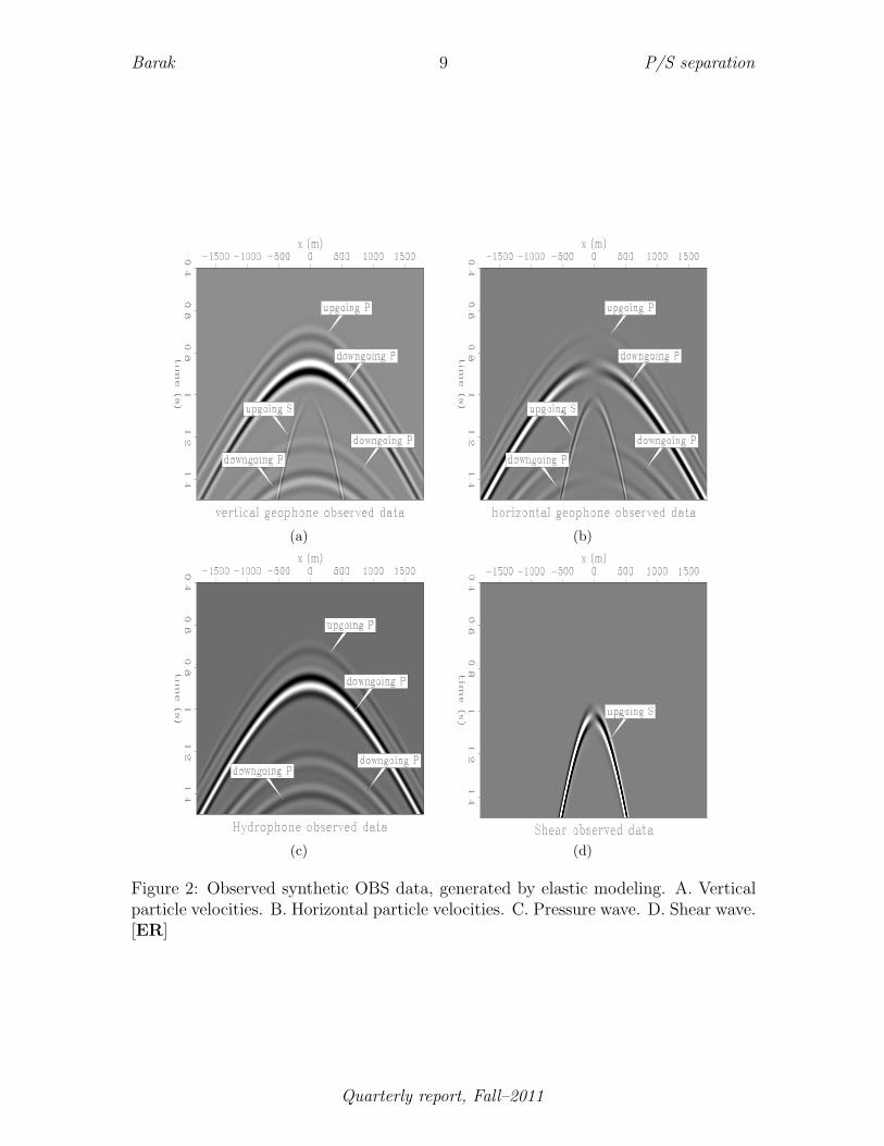
Synthetic data were modeled using a medium that contained a water column, overly-ing two horizontal layers with different elastic impedances. The upper boundary wasfree, so that reflections would occur as they do off the sea surface. The source was atthe sea surface, and the receivers were on the sea bed. This geometry simulates OBSacquisition.

The observed synthetic data is shown in Figures 2(a)-2(d). Note that the directarrival has been muted. Therefore, the first arrival in each panel of the figures is anupgoing P-wave. The arrival’s wave mode and propagation direction are designatedin the figures. The shear-wave in Figure 3(d) is not a representation of actual fielddata, but only serves to assist in the interpretation of the results.

The medium parameters which were used to generate the OBS synthetic data were:

1. P-wave velocity: vp1 = 1500ms, vp2 = 1700m

s, vp3 = 2000m

s

2. S-wave velocity: vs1 = 0ms, vs2 = 500m

s, vs3 = 800m

s

3. Density: ρ1 = 1.025gr/cm3 , ρ2 = 1.7gr/cm3 , ρ3 = 1.6gr/cm3

The inversion was run with virtual sources located below the receivers, in a homoge-neous medium with the following parameters:

1. P-wave velocity: vp = 1500ms

2. S-wave velocity: vs = 600ms

3. Density: ρ1 = 1.025gr/cm3

The virtual source array had the same length and number of injection points as thereceiver array.

Figures 3(a)-3(d) are the results of forward modeling of virtual-source models, whichwere produced after 200 iterations. Comparing Figures 2(a) and 2(b) to Figures

Quarterly report, Fall–2011

Barak 9 P/S separation

(a) (b)

(c) (d)

Figure 2: Observed synthetic OBS data, generated by elastic modeling. A. Verticalparticle velocities. B. Horizontal particle velocities. C. Pressure wave. D. Shear wave.[ER]

Quarterly report, Fall–2011

Barak 10 P/S separation

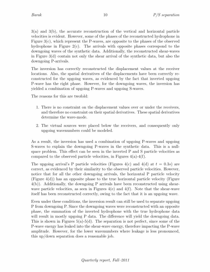
3(a) and 3(b), the accurate reconstruction of the vertical and horizontal particlevelocities is evident. However, some of the phases of the reconstructed hydrophone inFigure 3(c), which represent the P-waves, are opposite to the phases of the observedhydrophone in Figure 2(c). The arrivals with opposite phases correspond to thedowngoing waves of the synthetic data. Additionally, the reconstructed shear-wavesin Figure 3(d) contain not only the shear arrival of the synthetic data, but also thedowngoing P-arrivals.

The inversion has correctly reconstructed the displacement values at the receiverlocations. Also, the spatial derivatives of the displacements have been correctly re-constructed for the upgoing waves, as evidenced by the fact that inverted upgoingP-wave has the right phase. However, for the downgoing waves, the inversion hasyielded a combination of upgoing P-waves and upgoing S-waves.

The reasons for this are twofold:

1. There is no constraint on the displacement values over or under the receivers,and therefore no constraint on their spatial derivatives. These spatial derivativesdetermine the wave-mode.

2. The virtual sources were placed below the receivers, and consequently onlyupgoing wavenumbers could be modeled.

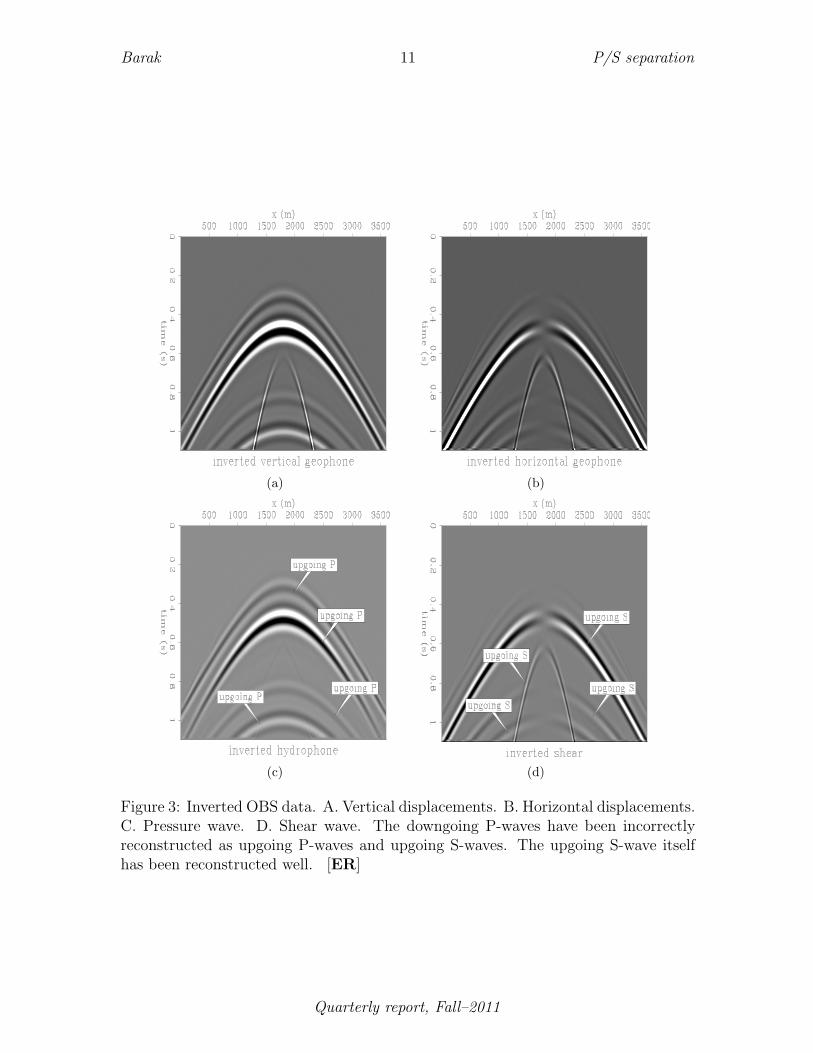
As a result, the inversion has used a combination of upgoing P-waves and upgoingS-waves to explain the downgoing P-waves in the synthetic data. This is a null-space problem. This effect can be seen in the inverted P and S particle velocities ascompared to the observed particle velocities, in Figures 4(a)-4(f).

The upgoing arrival’s P particle velocities (Figures 4(c) and 4(d) at t = 0.3s) arecorrect, as evidenced by their similarity to the observed particle velocities. However,notice that for all the other downgoing arrivals, the horizontal P particle velocity(Figure 4(d)) has an opposite phase to the true horizontal particle velocity (Figure4(b)). Additionally, the downgoing P arrivals have been reconstructed using shear-wave particle velocities, as seen in Figures 4(e) and 4(f). Note that the shear-waveitself has been reconstructed correctly, owing to the fact that it is an upgoing wave.

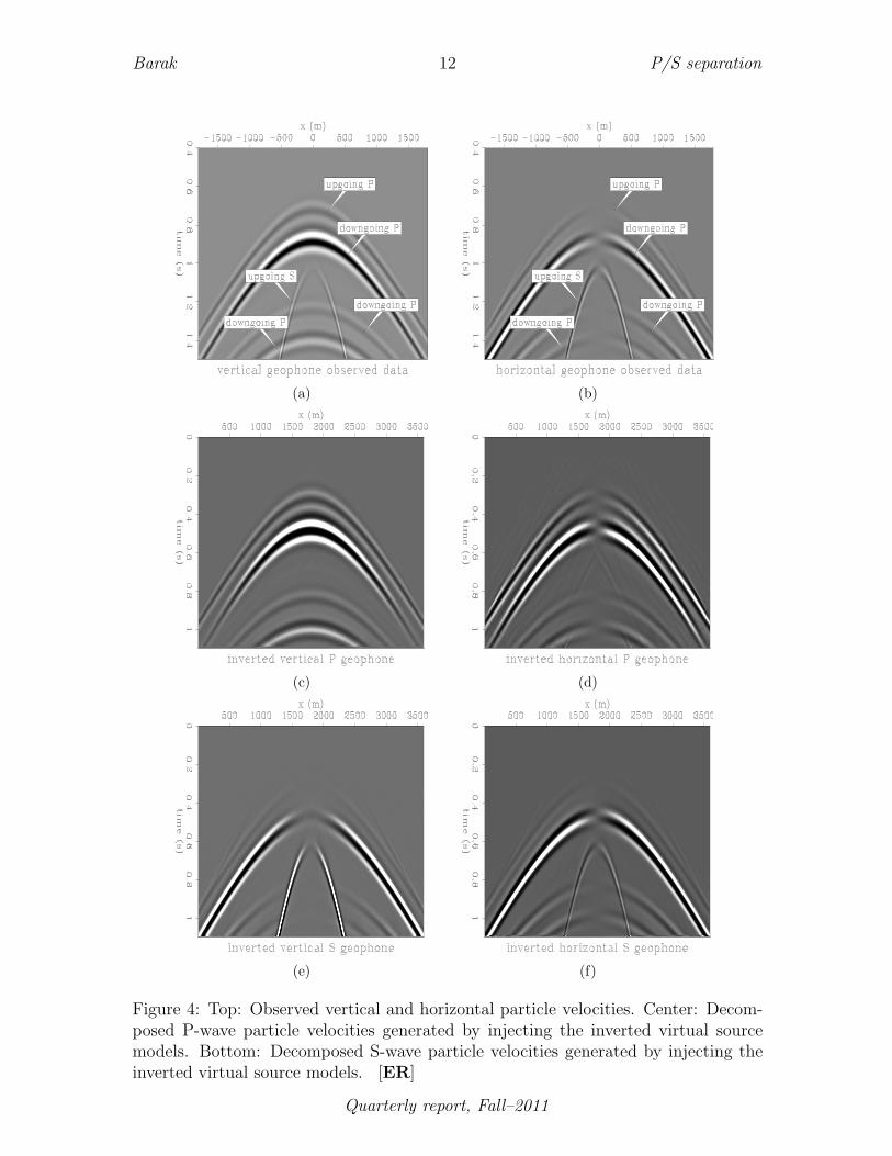
Even under these conditions, the inversion result can still be used to separate upgoingP from downgoing P. Since the downgoing waves were reconstructed with an oppositephase, the summation of the inverted hydrophone with the true hydrophone datawill result in mostly upgoing P data. The difference will yield the downgoing data.This is shown in Figures 5(a)-5(d). The separation is not perfect, since some of theP-wave energy has leaked into the shear-wave energy, therefore impacting the P-waveamplitude. However, for the lower wavenumbers where leakage is less pronounced,this up/down separation does a reasonable job.

Quarterly report, Fall–2011

Barak 11 P/S separation

(a) (b)

(c) (d)

Figure 3: Inverted OBS data. A. Vertical displacements. B. Horizontal displacements.C. Pressure wave. D. Shear wave. The downgoing P-waves have been incorrectlyreconstructed as upgoing P-waves and upgoing S-waves. The upgoing S-wave itselfhas been reconstructed well. [ER]

Quarterly report, Fall–2011

Barak 12 P/S separation

(a) (b)

(c) (d)

(e) (f)

Figure 4: Top: Observed vertical and horizontal particle velocities. Center: Decom-posed P-wave particle velocities generated by injecting the inverted virtual sourcemodels. Bottom: Decomposed S-wave particle velocities generated by injecting theinverted virtual source models. [ER]

Quarterly report, Fall–2011

Barak 13 P/S separation

(a) (b)

(c) (d)

Figure 5: A. Synthetic hydrophone data. B. Inverted hydrophone data. C. Syn-thetic+inverted hydrophone, resulting in mostly upgoing P-wave data. D. Synthetic-inverted hydrophone, resulting in mostly downgoing P-wave data. [ER]

Quarterly report, Fall–2011

Barak 14 P/S separation

DISCUSSION AND CONCLUSION

The inversion reliably recreates the observed geophone data at the receiver locations.

The dispositions of the virtual sources in relation to the receivers is a major factor indetermining which wavenumbers can be modeled by the inversion. If some wavenum-bers which exist in the field data cannot be modeled by a particular virtual sourcearray, then the inversion will strive to find another explanation for their existence.This explanation will utilize the null-space, and produce undesirable results. Theexample I show above indicates that for a simple virtual source arrangement that canproduce only upgoing waves, all downgoing P-wave displacements are explained by acombination of upgoing P-wave displacements and upgoing S-wave displacements.

This is related to the fact that though the particle motion at the receiver level iswell-constrained by the objective function, the vertical derivative of particle motionis not. Therefore, additional constraints must be used in the objective function, whichwill decrease the null-space.

My conclusion is that a correct combination of constraints and virtual source locationswill enable the inversion to recreate all wavenumbers correctly, and thus all wave-modes.

The P and S separation operator uses a second order in space finite-difference approx-imation to the first derivative. This low-order approximation can generate shear-waveartifacts on the separated P-wave data, and vice versa. Improving the approximationorder may reduce the artifacts. However, since a higher order approximation invari-ably uses a longer stencil, the effect of the recreated wavefield at greater distancesfrom the receivers will come into play. Since we can only assume that the wavefieldhas been reliably recreated near the receivers, a higher order approximation may notbe desirable.

REFERENCES

Amundsen, L., 1993, Wavenumber-based filtering of marine point-source data: Geo-physics, 58, 1497–150.

Barr, F. J. and J. I. Sanders, 1989, Attenuation of water-column reverberations usingpressure and velocity detectors in a water-bottom cable: SEG expanded abstracts,8, 653–656.

Claerbout, J. F. and S. Fomel, eds., 2011, Image estimation by example: Geophysicalsoundings image construction.

Dankbaar, J. W. M., 1985, Separation of p- and s-waves: Geophysical Prospecting,33, 970–986.

Dash, R., G. Spence, R. Hyndman, S. Grion, Y. Wang, and S. Ronen, 2009, Wide-areaimaging from obs multiples: Geophysics, 74, Q41–Q47.

Dellinger, J. and J. Etgen, 1990, Wave-field separation in two-dimensional anisotropicmedia: Geophysics, 55, 914–919.

Quarterly report, Fall–2011

Barak 15 P/S separation

Paffenholz, J., P. Docherty, R. Shurtleff, and D. Hays, 2006, Shear wave noise on obsvz data - part ii: Elastic modeling of scatterers in the seabed: EAGE extendedabstracts, 68th conference and exhibition, A072.

Ronen, S., L. Comeaux, and X. Miao, 2005, Imaging downgoing waves from oceanbottom stations: SEG expanded abstracts, 24, 963–966.

Schalkwijk, K. M., C. P. A. Wapenaar, and D. J. Verschuur, 2003, Adaptive decompo-sition of multicomponent ocean-bottom seismic data into downgoing and upgoingp- and s-waves: Geophysics, 68, 1091–1102.

Wapenaar, C. P. A., P. Herrmann, D. J. Verschuur, and A. J. Berkhout, 1990, De-composition of multicomponent seismic data into primary p- and s-wave responses:Geophysical Prospecting, 38, 663–661.

Wong, M., B. L. Biondi, and S. Ronen, 2009, Inversion of up and down going signalfor ocean bottom data: SEP-Report, 138, 247–256.

Zhang, Q. and G. McMechan, 2010, 2d and 3d elastic wavefield vector decompositionin the wavenumber domain for vti media: Geophysics, 75, D13–D26.

Zhou, Y., C. Kumar, and I. Ahmed, 2011, Ocean bottom seismic noise attenuationusing local attribute matching filter: SEG expanded abstracts, 81st annual meeting,3586–3590.

Quarterly report, Fall–2011