Preventing Behavior Problems in Childhood and Adolescence:

Evidence from Head Start∗

Pedro Carneiro

University College London,

Centre for Microdata Methods and Practice,

and Institute for Fiscal Studies

Rita Ginja†

University College London

July 2008

Abstract

This paper shows that participation in Head Start reduces the incidence of behavioral prob-lems, grade repetition, and obesity of children at ages 12 and 13, and depression, criminalbehavior, and obesity at ages 16 and 17. Head Start’s eligibility rules induce discontinuitiesin program participation as a function of income, which we use to identify program impacts.Since there is a range of discontinuities (they vary with family size, state and year), we identifythe effect of Head Start for the large set of individuals in the neighborhood of each of severaldiscontinuities, as opposed to a smaller set of individuals around a single discontinuity.

JEL Codes: C21, I28, I38.Keywords: Regression discontinuity design, early childhood development, non-cognitive skills,

Head Start.

∗We thank Joe Altonji, Sami Berlinski, Richard Blundell, Janet Currie, Michael Greenstone, Jeff Grogger, JamesHeckman, Isabel Horta Correia, Hilary Hoynes, Jens Ludwig, Costas Meghir, Robert Michael, Kevin Milligan, LarsNesheim, Jesse Rothstein, Chris Taber, Frank Wjindmeier, and seminar participants at IFS, the 2007 EEA Meetings,Universidade Catolica Portuguesa, Banco de Portugal, the 2008 RES Conference, the 2008 SOLE meetings, the 2008ESPE Conference and at the Annual Meeting of the Portuguese Economic Journal for valuable comments. PedroCarneiro gratefully acknowledges the financial support from the Leverhulme Trust and the Economic and Social Re-search Council (grant reference RES-589-28-0001) through the Centre for Microdata Methods and Practice, and thehospitality of the World Bank and Georgetown University. Rita Ginja acknowledges the support of Fundacao para aCiencia e Tecnologia.

†Address: Department of Economics, University College London, Gower Street, London WC1E 6BT, United King-dom. Tel.: +44 020 7679 5888, Fax: +44 020 7916 2775. E-mail: p.carneiro@ucl.ac.uk, r.ginja@ucl.ac.uk.

1

Where there’s a need for early intervention, we will work very intensively with those families so

that young people are deterred from going into gangs and guns and knife crime. Gordon Brown,

August 23, 2007, BBC News

To prevent: parents held accountable - fined if they fail to supervise. And so that these young

people are not left to hang around street corners, councils and authorities obligated to maintain their

education and supervision. Gordon Brown, September 24, 2007, Speech to Labour Conference

1 Introduction

Problem behaviors among adolescents are at the center of the social agenda in most developed coun-

tries. Faced with increasingly visible gang violence in the UK, prime minister Gordon Brown launched

a call for better parenting. While he is right in preferring prevention to remediation, and in asserting

that home environments are key for prevention, he will soon find out that they are incredibly hard to

change.

Early childhood programs for poor children have gained prominence as an alternative (e.g., Currie,

2001, Carneiro and Heckman, 2003). Model interventions such as Perry Preschool and Abecedarian

have proven to be effective in preventing behavioral problems (e.g., Barnett, 2004). The central

question is whether more universal (and less well funded) programs like Head Start in the US, or Sure

Start in the UK, can be equally successful.

In this paper, we study the impact of Head Start on behavioral problems of recent cohorts of

children and adolescents. We find strong program impacts on grade repetition, social behaviors (mea-

sured by a battery of behavioral questions), and obesity1 at ages 12-13; and on depression (measured

by a depression scale), crime, and obesity at ages 16-17. We account for self-selection into Head Start

using a (fuzzy) regression discontinuity design which explores program eligibility rules. We determine

eligibility to the program for each child by examining whether her family income is above or below

the income eligibility cutoff, which varies with year, state, family size, and family structure. Then

we check whether the relationship between family income and Head Start participation, outcomes at

1Obesity is usually seen as a health problem. While it is true that most of the effect of Head Start on this outcomeis probably due to nutrition education for children and parents, as well as other exercise and nutrition componentsof the program, there may also be a behavioral problem component to it. Frisvold (2007) and Frisvold and Lumeng(2008) show substantial effects of this program on obesity.

2

12-13, and outcomes at 16-17, is discontinuous at the income eligibility cutoff for each child.

The focus on behavioral problems is especially important given the controversy about the fade-

out of the effects of Head Start (and other early childhood programs) on the cognitive development

of children, especially that of blacks (see, e.g., Currie and Thomas, 1995, 1999). Recent research

argues that behavioral skills are more malleable than cognitive skills (Cameron, Heckman, Knudsen,

Schonkoff, 2006, Cunha and Heckman, 2006), and therefore more amenable to being affected by

policy (see, e.g., Carneiro and Heckman, 2003). Furthermore, behavioral problems in childhood and

adolescence are strong predictors of adult outcomes (e.g., Bowles, Gintis and Osborne, 2003, Heckman,

Sixtrud, and Urzua, 2006, Carneiro, Crawford and Goodman, 2007).

Our empirical strategy is novel in the study of Head Start. We implement it using the Children

of the National Longitudinal Survey of Youth of 1979 (CNLSY79), a survey with rich information

on children outcomes at different ages. In contrast with the standard regression discontinuity setup,

there are multiple discontinuity points, which vary across families because they depend on year, state,

family size and family structure. Therefore our estimates are not limited to individuals located around

a single discontinuity, but they are applicable to a more general population. The use of this dataset

also allows us to focus on recent program participants and answer questions about the impact of the

program in its present format.

Some recent evaluations of Head Start also address endogenous program participation (see Ludwig

and Phillips, 2007, for survey of the recent literature on Head Start.). Currie and Thomas (1995, 1999,

2000) use data from the CNLSY79 (the same dataset we use), and rely on sibling comparisons. They

find strong impacts of the program on a cognitive test (which fade-out for blacks, but not whites)

and grade repetition. Currie, Garces and Thomas (2002) use a similar strategy in the Panel Study of

Income Dynamics (PSID), and show that the program has long lasting impacts on adult schooling,

earnings, and crime. Ludwig and Miller (2007) explore a discontinuity in Head Start funding across

US counties induced by a federal assistance program in 1965. They show that Head Start positively

impacts children’s health and schooling. The latter two papers measure impacts of Head Start for those

who participated in the program in the 1960s and 1970s. More recently, Currie and Neidell (2007) use

CNLSY79 to study the quality of Head Start centers and find a positive association between scores

in cognitive tests and county spending in the program. They also find that children in programs that

3

devote higher shares of the budget to education and health have fewer behavioral problems and are

less likely to have repeated a grade. Frisvold and Lumeng (2007) explore an unexpected reduction in

Head Start funding in Michigan to show strong effects of the program on obesity. A recent randomized

control trial of Head Start has been commissioned by the US Congress. Only short run results are

available, but they show that the program improves cognitive and behavioral outcomes of 3 and 4

year old children. Finally, Neidell and Waldfogel (2006) argue that ignoring spillover effects resulting

from interactions between Head Start and non-Head Start children and/or parents underestimates

the effects of the program in cognitive scores and grade repetition.

Our paper adds to this literature in at least two important ways. First, we provide a systematic

study of the (medium to long term) impacts of Head Start on behavioral outcomes across different

ages, for those children participating in the program in the 1980s and 1990s. Second, we adopt a new

empirical strategy which explores detailed information on program eligibility rules. It differs from the

mother fixed-effects strategy used by Currie and Thomas (1995, 1999, 2000) and Currie, Garces and

Thomas (2002) by not requiring differences in Head Start participation across siblings to be random.

Instead, it assumes that households are unable to locate strategically just above or below the income

cutoffs that determine eligibility. This is a sensible assumption given the complexity of the eligibility

rules and the fact that they change over time. We also test and find no evidence of the existence

of any strategic behavior of this type. Our method is non-experimental, as opposed to US Congress

(2005), but allows us to follow up children until much later ages. Relatively to Ludwig and Miller

(2007), central differences are our focus on more recent participants into the program, our emphasis

on behavioral outcomes, and the fact that we explore more than one discontinuity.

This paper proceeds as follows. In the next section we describe the data we use. Then we discuss

the identification strategy in detail, and discuss several checks to the validity of the procedure. We

follow by presenting our empirical results. The last section summarizes and concludes.

2 Data

We use data on females from the National Longitudinal Survey of the Youth of 1979 (NLSY79)

combined with a panel of their children, the Children of the National Longitudinal Survey of Youth

4

of 1979 (CNLSY79). The NLSY79 is a panel of individuals whose age was between 14 and 21 by

December 31, 1978 (of whom approximately 50 percent are women). The survey has been carried out

annually since 1979 (interviews have become biennial after 1994). The CNLSY79 is a biennial survey

which began in 1986 and contains information about cognitive, social and behavioral development of

individuals (assembled through a battery of age specific instruments), from birth to early adulthood.

We focus on the impact of the program in two age groups.2 We study behavioral problems of

children 12 to 13 years of age using the Behavioral Problems Index scale, and an indicator for smoking

habits. We also examine behaviorally related measures of school success and health by looking at

an indicator of grade repetition, an indicator of special education attendance, and an indicator of

obesity. For adolescents 16 to 17 years of age we study mental health and motivational outcomes

using measures of depressive symptoms (the CESD), criminal behavior, smoking habits and obesity

(and in Appendix A we also present results for alcohol and marijuana use, high school enrollment,

and scores on cognitive tests.). A detailed description of the variables can be found in table A1 in

the Appendix A.

Since the CNLSY79 is a biennial survey there is only one observation per child in each two

consecutive years. Therefore, we group children in intervals of two consecutive ages in order to

maintain a reasonable sample size. The reason to focus on these age groups (and not earlier ones) is

that it is likely that behavioral problems become more obvious from early adolescence onwards, and

not so much before. We have checked earlier ages and results are indeed weaker.

Head Start is a preschool program that targets disadvantaged children and eligibility is means-

tested. Children 3 to 5 years of age are eligible to participate in the program if their family income is

below an income threshold, which varies with household characteristics, state of residence, and year.

Among the variables available in CNLSY79 there are those that determine income eligibility (total

family income, family size, state of residence, Head Start cohort and an indicator of the presence

of a father-figure in the child’s household3) along with outcomes at different ages of each child. All

monetary variables are measured in 2000 values using the CPI-U from the Economic Report of the

2We have also analyzed individuals ages 20-21. However, because sample sizes are small, results were too impreciseto be conclusive. These are available on request from the authors.

3Although father’s (or stepfather) employment is also a condition that determines Head Start eligibility, we didnot consider it, because the variable “number of weeks mother’s spouse worked” has missing values in half of theobservations. Inclusion of this variable and an indicator for missing values does not change the results.

5

President (2006). The earliest year in which we can construct eligibility at age four is 1979 (for children

born in 1975), since this is the first year in which income is measured in the survey. Similarly, since

we take outcomes measured at ages 12 and older, and the last year of data is 2004, the youngest

child in the sample is born in 1992. Therefore, we study the effects of participating in Head Start

throughout the 1980s and early 1990s. In section 3 we describe our procedure in detail.

Empirically, we distinguish three possible preschool arrangements: Head Start, other preschool

programs, or neither of the previous two (informal care at home or elsewhere). About 82 percent of

those mothers who report that their child was enrolled in Head Start, also report that their child was

enrolled in preschool, possibly confusing the two child care arrangements. Therefore, as in Currie and

Thomas (1995, 2000), we recode the preschool variable so that whenever a mother reports both Head

Start and preschool participation, we assume enrollment in Head Start alone (a detailed definition

of the alternative arrangements is given in section (4.2)). After recoding this variable, almost 21

percent of the children in the sample ever enrolled in Head Start, 44 percent attended other types of

preschool, and the remaining attended neither.4 In our data, about 70% Head Start participants are

in the program for one year only (or less).

It is well known that, as a consequence of the sample design, the children in CNLSY79 are

more deprived than the average American child. Given that not all mothers have yet completed their

fertility cycle, there is an oversampling of children from young mothers (because they are born earlier).

Additionally, roughly half of the original NLSY79 consists of an oversample of African-Americans,

Hispanics, and economically disadvantaged whites (and also a subsample of members of the military

which we exclude from our work).

As we explain in the next section, it is good practice to restrict the sample to children whose family

income at age four was near (in our case, between 5 and 195 percent of) the income eligibility cutoff

for the program since points away from the discontinuity should have no weight in the estimation

of program impacts (see Black, Galdo, and Smith, 2005, Imbens and Lemieux, 2007). Finally, in

4Based on official numbers we would expect the Head Start participation rate to be around 5% (20-25% of childrenin the US are poor, and 20-25% of poor children enrol in Head Start). One reason for having a larger estimate in ourdata may be the fact that we are using oversamples of minorities and poor whites, and more importantly, the fact thatwe overestimate children from young mothers. In fact, our number is comparable to the 19.4% figure in Currie andThomas (1995). Currie, Garces and Thomas (2000) estimate Head Start participation at 10% in the PSID, and Ludwigand Miller (2007) have participation rates of 20 to 40% in the counties close to their relevant discontinuity (based ondata from the National Educational Longitudinal Study).

6

this paper, we focus on male children only, for whom early behavioral problems are probably more

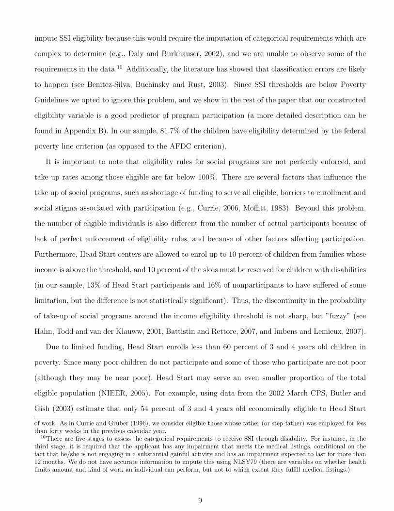
prevalent than for females.5 Table 1 summarizes the data. The full sample consists of 3029 males

for whom at least one of the measured outcomes is available and all the control variables used in the

regressions are not missing (child care arrangement at ages 3 to 5, eligibility to Head Start at age 4,

family log income and family size at age 4 and at ages 0 to 2, presence of a father or stepfather in the

household, state of residence at age 4, and birth weight).6.

Columns (1) and (2) of table 1 present means and standard deviations for the full sample and

in columns (3) to (10) we describe the restricted sample used in the regressions (household income

between 5 and 195% of the eligibility cutoff). Average family income is lower for individuals in the

restricted sample, and they also perform worse in all but one (probability of being overweight at

age 12 or 13) of the outcomes analyzed. Focusing on the relevant sample for our study, we have

1766 individuals. At ages 12 and 13, Head Start participants engage in more problem behaviors as

measured by the Behavioral Problems Index (BPI) than non-Head Start children; they are more likely

to have repeated a grade than non-participants by ages 12 and 13 (36% versus 32%), but they do not

show a strong propensity to be in special education, to be overweight, or to smoke, than children who

never enrolled in the program. There is a higher proportion of adolescents that have already been

sentenced of any charges or arrested among former participants relatively to non-participants (19%

versus 13%), but again not much of a difference in terms of depression (CESD), obesity, or smoking.7

As expected, participants come from families with lower income and who are more likely to be eligible

than non-participants. They belong to families where the father’s presence is infrequent, and who

are more likely to be below the poverty line than non-participants. Participants’ mothers have lower

cognitive ability measured by the Armed Forces Qualifying Test (AFQT), and the BPI is higher for

African-American children when compared to the rest of the sample.

5Unfortunately our results for females are very imprecise (available on request). The main reason is that, althougheligibility is a strong predictor of Head Start participation for males, it is much weaker for females. This is puzzlingsince males and females in our sample look exactly equal in all dimensions. We examined this carefully, but our resultswere inconclusive so we opted to leave a deeper study of this problem for future work.

6We exclude from the sample 22 children whose family size at age 4 is one since the children eligible for interviewin the survey are living at least part-time with their mothers.

7BPI is the Behavior Problems Index and it measures the frequency, range, and type of childhood behavior problemsfor children age four and over (Peterson and Zill, 1986). The Behavior Problems total score is based on responsesfrom the mothers to 28 questions that intent to measure (1) antisocial behavior, (2) anxiety and depression, (3)headstrongness, (4) hyperactivity, (5) immaturity, (6) dependency, and (7) peer conflict/social withdrawal. The CESD(Center for Epidemiological Studies Depression) Scale measures symptoms of depression and it discriminates betweenclinically depressed individuals and others.

7

3 Empirical Strategy

Our goal is to estimate β from the following equation:

Yi = α + βHSi + f (Xi) + εi (1)

where Yi is the outcome of interest for child i, which in our paper is measured at ages 12 to 13, or

16 to 17, HSi is an indicator of whether the child ever participated in Head Start, Xi is a vector of

controls (entering through function f (X)), and εi is an unobservable. β is the impact of Head Start

on Y which, in principle, can vary across individuals. Even if β is a common coefficient, estimation by

ordinary least squares (OLS) is problematic. Since Head Start participants are poor, they are likely

to have low levels of εi, inducing a negative correlation between HSi and εi. On the other end, not all

poor children participate in the program, and perhaps only the most motivated mothers enrol their

children, which would create a positive correlation between HSi and εi.

In order to address these problems we explore discontinuities in program participation (as a func-

tion of income) that result from its eligibility rules. Children ages 3 to 5 are eligible if either their

family income is below the federal poverty guidelines, or if their family is eligible for public assistance:

Aid to Families with Dependent Children (or AFDC, which became Temporary Assistance for Needy

Families, or TANF, after 1996) and Supplemental Security Income (or SSI; see D.H.H.S., 2007). We

construct poverty status by comparing family income with the relevant federal poverty line, which

varies with family size and year (Social Security Administration, 2006). Eligibility for AFDC requires

satisfying two income tests, and additional categorical requirements, all of which are state specific.

In particular, the gross income test requires that total family income must be below a multiple of

the state specific threshold, that is set annually and by family size at the state level.8 The second

income test that must be verified by applicants (but not by current recipients) is the countable income

test, that requires total family income minus some income disregards to be below the state threshold

for eligibility (U.S. Congress, 1994). In addition, AFDC families must obey a particular structure:

either they are female-headed families or families where the main earner is unemployed.9 We do not

8When this test was established in 1981 the multiple was set to 1.5. The Deficit Reduction Act of 1984 raised thislimit to 1.85 of the state need standard.

9Children in two-parents households may still be eligible to AFDC under the AFDC-Unemployed Parent program.Eligibility for AFDC-UP is limited to those families in which the principal wage earner is unemployed but has a history

8

impute SSI eligibility because this would require the imputation of categorical requirements which are

complex to determine (e.g., Daly and Burkhauser, 2002), and we are unable to observe some of the

requirements in the data.10 Additionally, the literature has showed that classification errors are likely

to happen (see Benitez-Silva, Buchinsky and Rust, 2003). Since SSI thresholds are below Poverty

Guidelines we opted to ignore this problem, and we show in the rest of the paper that our constructed

eligibility variable is a good predictor of program participation (a more detailed description can be

found in Appendix B). In our sample, 81.7% of the children have eligibility determined by the federal

poverty line criterion (as opposed to the AFDC criterion).

It is important to note that eligibility rules for social programs are not perfectly enforced, and

take up rates among those eligible are far below 100%. There are several factors that influence the

take up of social programs, such as shortage of funding to serve all eligible, barriers to enrollment and

social stigma associated with participation (e.g., Currie, 2006, Moffitt, 1983). Beyond this problem,

the number of eligible individuals is also different from the number of actual participants because of

lack of perfect enforcement of eligibility rules, and because of other factors affecting participation.

Furthermore, Head Start centers are allowed to enrol up to 10 percent of children from families whose

income is above the threshold, and 10 percent of the slots must be reserved for children with disabilities

(in our sample, 13% of Head Start participants and 16% of nonparticipants to have suffered of some

limitation, but the difference is not statistically significant). Thus, the discontinuity in the probability

of take-up of social programs around the income eligibility threshold is not sharp, but ”fuzzy” (see

Hahn, Todd and van der Klauww, 2001, Battistin and Rettore, 2007, and Imbens and Lemieux, 2007).

Due to limited funding, Head Start enrolls less than 60 percent of 3 and 4 years old children in

poverty. Since many poor children do not participate and some of those who participate are not poor

(although they may be near poor), Head Start may serve an even smaller proportion of the total

eligible population (NIEER, 2005). For example, using data from the 2002 March CPS, Butler and

Gish (2003) estimate that only 54 percent of 3 and 4 years old economically eligible to Head Start

of work. As in Currie and Gruber (1996), we consider eligible those whose father (or step-father) was employed for lessthan forty weeks in the previous calendar year.

10There are five stages to assess the categorical requirements to receive SSI through disability. For instance, in thethird stage, it is required that the applicant has any impairment that meets the medical listings, conditional on thefact that he/she is not engaging in a substantial gainful activity and has an impairment expected to last for more than12 months. We do not have accurate information to impute this using NLSY79 (there are variables on whether healthlimits amount and kind of work an individual can perform, but not to which extent they fulfill medical listings.)

9

in 2001 were served by the program. Additionally, families’ characteristics change over time, making

it difficult to estimate the size of the targeted population in each year and to identify all eligible

children. Imperfect compliance is not unique to Head Start, but common across social programs.11

A child can enrol in Head Start at ages 3, 4, or 5 and it is possible to construct eligibility at each

of these ages. However, for implementing the estimator it is convenient to pick an age. In our data

eligibility at age 4 is a better predictor of program participation than either eligibility at 3 or at 5,

and most children enrol in Head Start when they are 4 (U.S. Congress, 2004). Therefore we focus on

eligibility at age 4 in our main specification, but we also present results with eligibility at other ages.

Unfortunately, nonparametric estimation (as proposed in Hahn, Todd and van der Klauww, 2001,

Porter, 2003, and Imbens and Lemieux, 2007), is not practical in our setting because of multiple

discontinuities and small sample, which makes it difficult to implement a nonparametric estimator

for each discontinuity.12 Instead, we rely on series estimation, as in Angrist and Lavy (1999), Lee

and DiNardo (2004), and Chay, McEwan and Urquiola (2005), restricting the sample to values of the

forcing variable that are not far off the highest and the lowest cutoff points.

For simplicity, we start by estimating the following reduced form model:

Yi = φ + γEi + f (Zi, Xi) + ui (2)

where Ei is an indicator of eligibility for Head Start, Xi is a set of determinants of eligibility for each

child (year, state, family size, family structure, measured at age 4), Zi is family income (at age 4),

and ui is the unobservable. The equation for Ei is:

Ei = 1[Zi ≤ Z (Xi)

], (3)

where 1 [.] denotes the indicator function. f (Zi, Xi) is specified as a parametric but flexible function,

and Z (Xi) is a deterministic (and known) function that returns the income eligibility cutoff for a

11Only 2/3 of eligible single mothers used AFDC (Blank and Ruggles, 1996); 69 percent of eligible households forthe Food Stamps program participated in 1994 (Currie, 2006); of the 31 percent of all American children eligible forMedicaid in 1996, only 22.6 percent were enrolled (Gruber, 2003); EITC has an exceptionally high take-up rate of over80 percent among eligible taxpayers (Scholz, 1994); in 1998, participation in WIC (the Special Supplemental NutritionProgram for Women, Infants and Children) among those eligible was 73 percent for infants, 2/3 among pregnant womenand 38 percent for children (Bitler, Currie and Scholz, 2003).

12One could also think of recentering all the data relatively to the relevant cutoff. Some experiments with thisstrategy show very similar results to the ones we present here (see the discussion in section 4.2).

10

family with characteristics Xi (constructed from the eligibility rules). At the end of the next section

we study the sensitivity of our results to the choice of different functional forms for f (Zi, Xi). We use

probit models whenever the outcome of interest is binary (the linear probability model is especially

inadequate when mean outcomes are far from 50 percent; see Table 1).

Three conditions need to hold for γ to be informative about the effects of Head Start on children

outcomes. First, after controlling flexibly for all the determinants of eligibility, Ei must predict

participation in the program, which we show to be true. One problem is that, at first sight, the

control group is not clearly defined, since we consider two alternatives to Head Start: preschool, and

home (or informal) care. Below we show that individuals induced to enter into Head Start because

of a shift in eligibility status come almost exclusively out of home (or other informal) care, giving us

a clear control group.

Second, families are not able to manipulate household income around the eligibility cutoff. This

is the main assumption behind any regression discontinuity design. It is likely to hold in our case

because the formulas for determining eligibility cutoffs are complex, and depend on family size, family

structure, state and year, making it difficult for a family to position itself just above or just below the

cutoff.13 Still, in order to guard against the possibility of income manipulation, there are standard

ways to test for violations of this assumption (e.g., Imbens and Lemieux, 2007), and below we discuss

them in detail.

Third, eligibility to Head Start should not be correlated with eligibility to other programs that

also affect child outcomes. This assumption is less likely to hold than the first two, because there

are other means tested programs which have eligibility criteria similar to those of Head Start (e.g.,

AFDC, SSI, or Food Stamps). Below we show that these other programs are unlikely to be important

determinants of children’s behavioral problems. We implement the following test. While most welfare

programs exist throughout the child’s life, Head Start only exists when the child is between the ages

of 3 and 5. If other programs affect behavioral problems of children, then eligibility to those programs

in ages other than 3 to 5 should also affect children’s outcomes. In contrast, if eligibility is correlated

with children’s outcomes only when measured between ages 3 and 5, then it probably reflects the

13For example, if we focus solely on the federal poverty line for a family of 4, between 1990 and 2000 it took thefollowing values: 12700, 13400, 13950, 14350, 14800, 15150, 15600, 16050, 16450, 16700, 17050. The AFDC cutoffs arestate specific and also vary over time.

11

effect of Head Start alone.

Below we implement these tests and we find no evidence that: i) families strategically manipulate

their incomes; and ii) other programs are confounding the impact of Head Start.

In practice, γ does not correspond to the impact of Head Start on the outcome of interest, because

eligibility does not fully predict participation (imperfect compliance). In order to determine the

program impact, we estimate the following system for continuous Yi:

Yi = α + βHSi + g (Zi, Xi) + εi (4)

HSi = 1 [η + τEi + h (Zi, Xi) + vi > 0] , (5)

where equation (5) is estimated using a probit model (van der Klauww, 2002). In practice, Pi =

Pr (HSi = 1|Ei, Zi, Xi) is estimated in a first stage regression, and used to instrument for HSi in

a second stage instrumental variable regression (van der Klauww, 2002, Hahn, Todd and van der

Klauww, 2001). If Yi is binary we use a bivariate probit. g (.) and h (.) are flexible functions of

(Zi, Xi).

Relatively to the standard case, the variability in the eligibility cutoff shown in Figure 1 provides

additional variation. Figure 1 displays the density of discontinuities in our data. This ”continuum

of discontinuities” allows us to go beyond the traditional regression discontinuity design and identify

treatment effects for individuals over a wide range of values for income and family size (the two

main running variables). Black, Galdo and Smith (2005) also recognize the potential of multiple

discontinuities to identify heterogeneous effects of the program.

Therefore, we can consider models where β varies explicitly across individuals:

Yi = α + βiHSi + g (Z i, Xi) + εi. (6)

If there is perfect compliance, in the sense that HSi = Ei, then Hahn, Todd and van der Klauww

(2001) show that using regression discontinuity we can estimate E(βi|Zi = Zi, Xi

)(the average

effect of the program conditional on Z) over the support of Z in the data. Under the weaker

condition that HSi = Ei only when Ei = 0, we estimate E(βi|Zi = Zi, Xi, HS = 1

)(Battistin

and Rettore, 2007). More generally, one can have non-compliance on both sides of the disconti-

12

nuity, in which case we obtain an estimate of a Local Average Treatment Effect (LATE; Imbens

and Angrist, 1994) at Zi = Zi, over the support of Z (the set of income eligibility cutoffs), or

E(βi|HS

(Zi − δi

)−HS

(Zi + δi

)= 1, Xi, Zi = Zi

), for δi > 0. The latter is the case in our data.

There are two reasons why this parameter may vary with Z: i) βi is a function of Zi (income at the

time eligibility is measured); or ii) even if there is independence between βi and Zi in the sample,

independence may not hold conditional on program participation if HSi depends on βi.14 In our

setting, it is impossible to distinguish the two.

We implement this estimator as follows. Say βi = h (Zi, Xi) + ui (where h is a flexible function of

X and Z, and ui is independent of (Xi, Zi)). Then, for each value of Z in the support of Z:

E(βi|HS

(Zi − δi

)−HS

(Zi + δi

)= 1, Xi, Zi = Zi

)= h

(Zi, Xi

)+ E

(ui| − η − τ − h

(Zi, Xi

)< vi ≤ −η − h

(Zi, Xi

))= h∗

(Zi, Xi

).

We recover this object by estimating the following system:

Yi = α + h∗ (Zi, Xi) ×HSi + g (Zi, Xi) + εi (7)

HSi = 1 [η + τEi + h (Zi, Xi) + vi > 0] . (8)

For simplicity, we model h∗ (Zi, Xi) as:

h∗ (Zi, Xi) = β0 + β1 × (family (log) income at age 4)i

+β2 × (family (log) income at age 4)2i + β3 × (family size at age 4)i + β4 × (family size at age 4)2

i

+β5 × (family (log) income at age 4)i × (family size at age 4)i.

Potentially we would like to estimate h∗ (Zi, Xi) using a more flexible specification, but our sample

size forces us to be parsimonious. We report estimates of β0, β1, β2, β3, β4 and β5, as well as estimates

14Say program participation is determined by equation (5), and βi is correlated with vi. Even if βi is independent ofZi,

E[βi|HS

(Zi − δi

)−HS

(Zi + δi

)= 1, Xi

]= E

[βi| − η − τ − h

(Zi, Xi

)< vi ≤ −η − h

(Zi, Xi

), Xi

],

which is a function of Zi. Intuitively, the set of vi for individuals at the margin varies with the level of Zi.

13

of the average partial effect of Head Start. We also display graphical representations of h∗ (Zi, Xi).

As before, equation (8) is estimated assuming vi has a normal distribution (probit). Whenever Yi is a

discrete outcome we assume that εi is also normal, and estimate the system using a bivariate probit.

Even with such parsimonious specification our estimates of this function in the next section are quite

imprecise, and results should be seen as suggestive and illustrative of the potential of this approach.

4 Results

4.1 Validity of the Procedure

Our identifying assumption in this setting is that children just above the income eligibility cutoff are

equal to those just below it in all dimensions except program participation. A priori this is a plausible

assumption, since it is very difficult for any family to purposely locate just below (or just above) the

eligibility cutoff in order to gain access to the program. Still, there are strong incentives for a family to

behave this way. For example, a family just above the income cutoff could try to underreport income

in order to become just eligible. Similarly, Head Start providers who know the eligibility rules well,

and who have a desire to serve children who are easy to care for, may try to game the system in order

to accept a large proportion of those children who are just ineligible. Fortunately, there are several

sources of information on which we can draw on to understand the importance of these concerns.

We start this section with a standard test of the validity of our identification assumptions. We take

a set of pre-program variables that should not be affected by participation in the program, and we use

them as dependent variables in equation (2). If our procedure is valid then the estimate of γ should

be equal to zero. These variables are: birth weight, whether the child was breastfed, mother’s age at

child’s birth, mother’s AFQT score, mother’s education, and average log family income and family size

between the ages of 0 and 2. Eligibility is measured at age 4, as explained above. f (Zi, Xi) consists

of fourth order polynomials in log family income and family size at age 4, an interaction between

these two variables, a dummy indicating the presence of a father figure (father or step-father) in the

household at age 4, gender, race and age dummies, and dummies for year and state of residence at age

4. Panel A of table 2 presents the results for the whole sample, while panel B focuses on blacks only.

Results for the older group (16-17) are similar (and available from the authors). Unless mentioned

14

otherwise, all standard errors in the paper are clustered at the level of the mother, since each mother

may have more than one child in the sample.15

Table 2 shows that our procedure is valid. Most estimates of γ are small (compared with the mean

and standard deviation of each variable in table 1), and all of them are statistically insignificant. In

order to better understand the magnitude of these estimates we conducted the following exercise.

Take a few of our main outcomes of interest, such as BPI and grade repetition at ages 12-13, and ever

sentenced by ages 16-17. Then regress each outcome on each of the variables in table 2 (one regression

per column), and compute predicted values for each regression. We can now rerun the regressions

on table 2 using these predicted values instead of the variables that generated them, allowing us to

translate the coefficients in table 2 into magnitudes of the outcomes of interest. We do not report

this in a table, but describe the results briefly: in terms of BPI, all the coefficients in table 2 are

between -0.017 and 0.011 (expressed as a fraction of a standard deviation), for grade repetition they

are between -1.4 and 1.8 percentage points (grade repetition has a mean of about 35%), and for ever

sentenced up to ages 16 to 17 they are between -0.6 and 0.5 percentage points (ever sentenced has a

mean of about 15%). All these figures are very small. Throughout the rest of the paper we augment

our basic specification of f (Zi, Xi) with some of the variables in table 2 as additional covariates, since

they are useful to reduce sampling error and small sample bias (e.g., Imbens and Lemieux, 2007).

In particular, we add fourth order polynomials in average log family income and average family size

between ages 0 and 2, an interaction between the two, and a fourth order polynomial in birth weight.16

15Column ”All” of Tables A2.1 and A2.2 in Appendix presents estimates when our specification includes an extendedset of controls. In particular, besides the controls included in our ”Basic” specification (fourth order polynomials in logfamily income and family size at age 4, an interaction between these two variables, a dummy indicating the presenceof a father figure in the household at age 4, fourth order polynomials in average log family income and average familysize between ages 0 and 2, an interaction between the two, and a fourth order polynomial in birth weight, race and agedummies and dummies for year and state of residence at age 4), we also add polynomials up to the fourth order onmother’s AFQT, on mother’s age at child’s birth, on mother’s highest grade completed when child was three years oldand an indicator for whether the child was breastfed. We do not use the full set of controls in table 2 because in suchan extended specification our results are slightly more imprecise, although they have similar magnitude and sign.

16An alternative and more direct test, developed by McCrary (2007), checks whether there is bunching of individualsjust before the discontinuity. This test is not practical with multiple discontinuities unless we have a large sample size.However, when we implemented it using a single discontinuity (using percentage distance to the eligibility cutoff asthe running variable) we found no evidence of income manipulation. Moreover, since we have panel data on maternalincome we can check whether there is direct evidence of income manipulation. Our assumption is that if mothers areunderreporting income for the purposes of becoming eligible for Head Start, then they are also likely to be underreportingincome in the survey. In addition, if they are far away from the discontinuity, they have no incentive to missreportincome. Under these conditions, if manipulation of income close to the income eligibility cutoffs was an empiricallyimportant phenomenon then we would expect income to be unexpectedly low whenever the mother is just below thecutoff. In order to test this formally we run a regression of family income on child fixed effects, dummies for year andage of the mother, and a dummy indicating whether the child is just below the income eligibility cutoff (more precisely,

15

4.2 Estimates from the Reduced Form Equations

We proceed by checking whether the discontinuity in eligibility status also induces a discontinuity in

Head Start participation, by estimating equation (5) (participation equation). We present estimates

for the main sample described above, and for a sample of black children, for whom behavior problems

are likely to be especially serious. Table 3 shows estimates of τ in equation (5), and for the average

marginal change in participation as the eligibility status varies, which is defined by:

1

N

N∑i=1

{Pr (HSi = 1|Ei = 1, Zi, Xi) − Pr (HSi = 1|Ei = 0, Zi, Xi)} =

1

N

N∑i=1

[Φ(η + τ + h

(Zi − δi ≤ Zi ≤ Zi + δi, Xi

)) − Φ(η + h

(Zi − δi ≤ Zi ≤ Zi + δi, Xi

))]

which we call the ”mean change in marginal take-up probability” (where N is the number of children

in the sample, and Φ is the standard normal c.d.f.).17

Each set of columns in table 3 corresponds to a different age group. The top panel refers to the

whole sample, while the bottom panel refers only to blacks. For each outcome we present estimates

of τ in a model without controls (columns 1 and 3), and in a model with all the control variables

(columns 2 and 4). Across ages and samples, eligibility is a strong predictor of program participation,

although the estimated effect is well below 100%. This is an indication of weak take-up of the program

at the margin of eligibility (common to many social programs), which could be a result of several

factors, such as lack of available funds to cover all eligible children (since Head Start was never fully

funded), stigma associated with program participation (Moffitt, 1983), or the fact that most of the

centers are only part-day programs, and thus unable to satisfy the needs of working families (Currie,

2006).18

her family income corresponds to 90 to 99% of the income eligibility cutoff). In results available on request we find noevidence that there is underreporting just below the cutoff. Oddly, if anything, the opposite is true. This conclusionholds even if we add to this regression a dummy indicating whether the child is between the ages of 3 and 5, and weinteract it with the dummy indicating whether the child is just below the cutoff. These tests are available from theauthors.

17In results not presented in the paper, we also estimate this effect at the median of the distribution of effects, as wellas the effect averaged over the set of individuals whose family income was between 75 and 125 percent of the incomediscontinuity. All the estimates produced the same results.

18Our paper is novel in obtaining estimates of Head Start take-up for individuals near the eligibility threshold asthe eligibility status change (although we consider a continuum of eligibility thresholds). Most of the evidence of hownewly eligible to social programs respond in terms of participation comes from Medicaid expansions throughout the1980s and early 1990s. Cutler and Gruber (1996) and Currie and Gruber (1996) estimate that only 23 and 34 percentof newly eligible children and women of childbearing age take-up Medicaid coverage, as many were already covered by

16

Table 3 shows how Head Start participation responds to eligibility, but it also raises the following

question: in which type of child care would children enrol in the absence of the program? The answer

is crucial for interpreting the results, since it defines the ”control group” in our study. While it is

possible to reconstruct the child care experiences during the first three years of life for all children

from mothers’ reports, for children aged 3 to 5 (when Head Start is available) the information about

child care arrangements is less detailed. The information we use is the following. Since 1988 child

surveys include questions, posed to the mother for children three years of age or older on whether

the children attend nursery school or a preschool program or had ever been enrolled in preschool, day

care, or Head Start. Using the age when first attended Head Start and the length of time attending we

construct an indicator of Head Start attendance between ages 3 to 5. This is our treatment variable.19

We recover information about preschool attendance from the question ”Ever enrolled in preschool?”.

The alternative child care arrangements between ages 3 to 5 we consider are:

HSi = 1[Ever in Head Start between ages 3 to 5]

OPi = 1[Ever enrolled in preschool but not in Head Start]

Homei = 1[Never in Head Start or in any other preschool]

where 1[.] is the indicator function (Homei denotes any other child care arrangement). Table 4 shows

how participation in the three alternative child care arrangements respond to eligibility. We regress

the dummy variables indicating participation in each type of child care on eligibility and the remaining

control variables, as in Table 3. Across age and race groups, when an individual becomes Head Start

eligible there is only a statistically significant movement out of Home Care and into Head Start.

Therefore we interpret our estimate of β (from equation (4)) as the effect of Head Start relatively to

Home care.20

other insurance. In our sample, 40.4% percent of those eligible at age four who did not attend Head Start were enrolledin another preschool program. Card and Shore-Sheppard (2002) find that expansion of Medicaid eligibility to childrenwhose family income was below 133 percent of the poverty line had no effects on the decision of take-up, whereasthe expansion of eligibility to all poor children led to an increase of nearly 10 percent in Medicaid coverage. LoSassoand Buchmueller (2002) estimate that take-up rates among newly eligible children for SCHIP (State Children’s HealthInsurance Program) ranged between 8 and 14 percent.

19The questions used to construct the indicator of Head Start attendance are: ”Child ever enrolled in Head Startprogram?”, ”Child’s age when first attended Head Start?” and ”How long was child in Head Start?”.

20The estimates for the marginal change in the take-up of the three child care alternatives do not change if amultinomial logit model is estimated instead of separate probit models for each choice. For the sample of all children 12and 13 years old the mean of individuals’ marginal effect of eligibility at age 4 on ”Head Start” is 0.136, the marginal

17

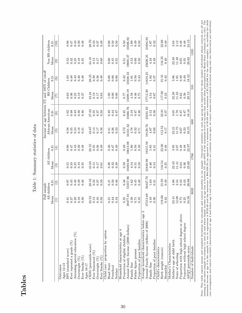
Tables 5 and 6 are the central tables of our paper. They present estimates of equation (2) (a

regression of outcome on eligibility) for the main set of outcomes. Table 5 refers to ages 12-13, and

table 6 refers to ages 16-17. Again, we consider two specifications for each outcome: one without

control variables (not controlling for selection), and one with all the controls (where the reported

coefficient corresponds to an “intent to treat” estimate). In the first column we expect to see eligible

children having worse outcomes than ineligible children, because they are in poorer households. In

the second column we will have an estimate of the impact of the program. Recall that we restrict the

sample to children whose family income is between 5% and 195% of the income eligibility cutoff (this

excludes middle and high income children).

The first column of table 5 shows that eligible children have a Behavior Problems Index which

is 0.15 of a standard deviation worse than ineligible children. Columns 3, 5, 7 and 9 also show

that they have much higher rates of grade repetition (7.4 percent higher among eligible children),

and enrolment in special education (4.8 percent higher among eligible), while there is no apparent

difference in obesity. In contrast, the estimates in the second column for each outcome document

that, as a result of Head Start eligibility, problem behaviors improve by ages 12-13, the probability

of grade repetition decreases on average by 11.6%, and the incidence of obesity is reduced by 8%.

Among blacks, the program only appears to have a strong effect on obesity, and it has an unexpected

negative impact on enrolment in special education. The latter may be just the result of sampling

error, given that both at ages 10-11, and 14-15, the coefficient is negative, as expected (available from

the authors).

Table 6 shows that, if we do not account for selection into Head Start, eligible adolescents are

more likely to have been sentenced for a crime by ages 16 to 17 (either in the entire sample and for

Blacks) and more likely to ever have smoked. Once selection is appropriately accounted for, Head

Start improves the incidence of depression in late adolescence (measured by CESD) as well as obesity.

When we focus on blacks, the strongest effect is on the probability of ever being sentenced up to

the age of 16-17 (a decrease of 18%). Tables A2.1 and A2.2 in Appendix A show (for a selected

set of outcomes) that these results are robust to the degree of the polynomial we choose to specify

effect on ”Other Preschool” is 0.13, and for ”Home” the marginal effect is -0.266. Among Black children the marginaleffects of eligibility on each alternative are 0.18, 0.106 and -0.295 for ”Head Start”, ”Other Preschool” and ”Home”,respectively. Similar results were found for the sample of 16-17 years individuals and are available from the authors.

18

g (Zi, Xi), whereas table A3 shows robustness to the size of the window of data chosen around the

discontinuity, and table A4 reports the partial effects (and standard errors) when we allow f (Zi, Xi)

in equation (2) to be a different function in either side of the discontinuity. Notice that the latter

case allows for heterogenous effects of the program as the ”Effect at Mean” is a function of the child’s

income threshold, which in turn depends on a bundle of observable family characteristics (see section

(3)).21 When we allow for different specifications on either side of the threshold estimates become

quite imprecise, although they have the same sign and roughly similar magnitudes to the ones we

report here.22 Therefore we proceed with the simpler and more robust specification.

In appendix table A5 we analyze the following additional outcomes at ages 16 and 17: alcohol and

marijuana use and enrolment in school. We were not able to reject the hypothesis that Head Start

had no impact in each of these outcomes, although in some cases standard errors were too large for

our estimates to be informative. In the appendix we also present estimates of equations (5) and (2)

for the sample of non-black males (tables A6 to A8), which are similar to the ones we report in the

main text, but with a weaker ”first stage” relationship.

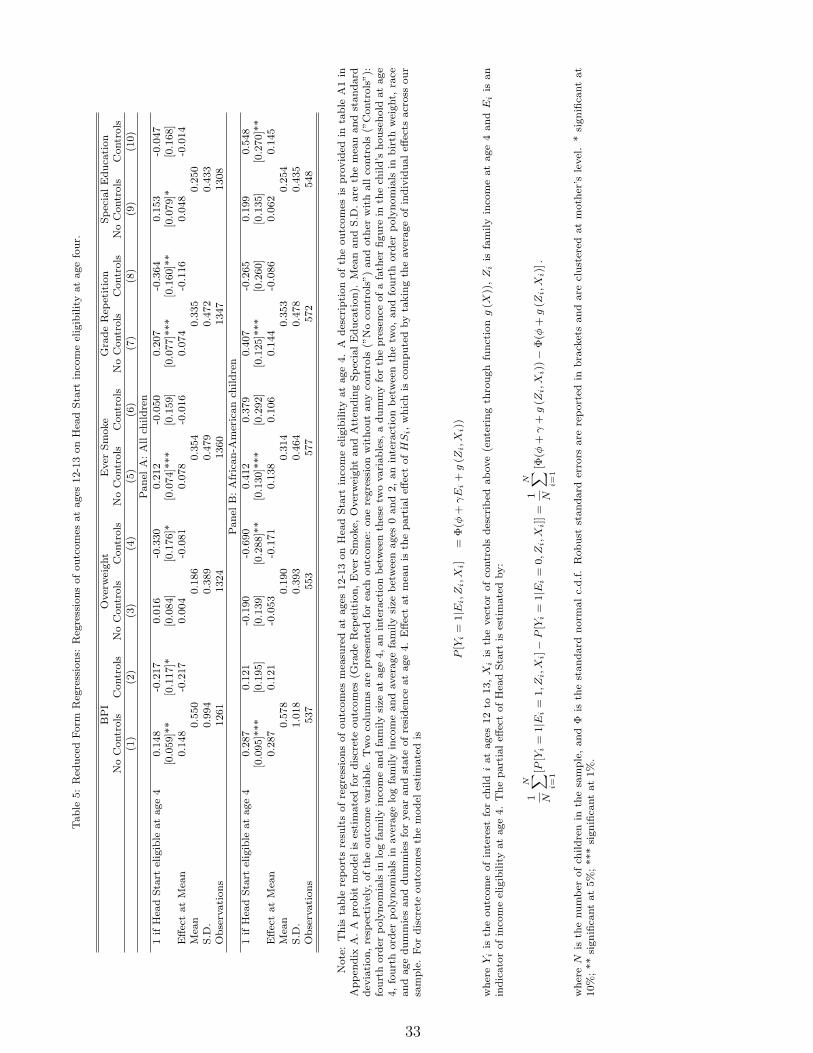
It is standard practice to also present a graphical analysis of the problem. However, the standard

setting has a single discontinuity and, since our setup makes use of a range of discontinuities, this

is not practical. One alternative that does not correspond exactly to the specification of our model

is, as mentioned above, to measure every household’s income relatively to their income eligibility

cutoff, and define the variable distance to the eligibility cutoff. In the appendix we plot Head Start

participation (figures A1 and A2, for ages 12-13 and 16-17, respectively) and some selected outcome

variables (figures A3, A4, A5, A6, A7, A8, A9) against distance to the eligibility cutoff as a percentage

of the income cutoff for the samples we use in our main specifications. We divide the sample into

bins of this variable (size equal to 9.5%) and compute cell means for the variable of interest, we draw

a vertical line at zero (point of discontinuity), and we run local linear regressions of each variable on

distance to cutoff on either side of the discontinuity (bandwidth = 0.3).

The figures suggest that there are large discontinuities in program participation at the eligibility

21The ”Effect at Mean” is computed obtained by: E[Yi|Zi = Z (Xi)− δ

]−E

[Yi|Zi = Z (Xi) + δ

]= γ+h(Z (Xi)).

See note of table A4 for details on the model estimated.22Standard errors for the estimated ”Effect at Mean” are also presented in table A4. These were obtained by 249

bootstrap replications. We use the non overlapping block bootstrap procedure described in Lahiri (1999). Blocks aredefined by mother.

19

cutoff. There are also discontinuities in the level of most outcomes, generally with the same sign as

in the tables above. The most important difference is in the variable ever sentenced for blacks, which

shows a strong impact of the program in the table (which is quite robust, as seen above) but not in

the figure. It is possible that the differences can be attributed to different specifications of the model

and small sample: use of household income vs. distance to the eligibility cutoff as a percentage of

the cutoff. In this setting we prefer the former specification because it corresponds more closely to a

simple economic relationship (between inputs and outputs).

As mentioned in section 3, eligibility to Head Start is correlated with eligibility to other programs,

such as AFDC, Medicaid, or SSI. It is therefore possible that the estimates in tables 5 and 6 confound

the effects of Head Start with those of other programs.23 However, while most of these programs exist

during several years of the child’s life, Head Start is only available when the child is between ages 3

and 5. This fact allows us to assess whether confounding effects from other programs are important.

Our reasoning is as follows. Suppose that we estimate equation (2) using eligibility (as well as the

covariates) measured at different ages of the child. If participation in other programs is driving our

results, Ei should have a strong coefficient even when measured at ages other than 3 to 5. Otherwise,

we can be confident that our estimates reflect the impact of Head Start, since it is unlikely that other

programs affect child development only if the child enrols at ages 3 to 5, but have no effect if she

enrols either at ages 0, 1 and 2 or at ages 6 and 7.

This reasoning will work if the set of individuals who are at the margin of eligibility at ages 3

to 5, are different from those who are at the margin of eligibility at ages 0, 1, 2, 6 and 7. If they

were all the same individuals it would be impossible to distinguish eligibility to Head Start (only

at ages 3 to 5) from eligibility to other programs (at all ages). Table 7 presents estimates for a

representative set of outcomes, one for each panel (the remaining outcomes show the same patterns,

and are available from the authors). Each column represents a different regression, where the age of

eligibility (and the corresponding controls) goes from 0 to 7. Across panels, the largest and strongest

estimates occur consistently at age 4, and sometimes 5 (grade repetition in panel A1, probability of

being overweight among children in panels A2 and B2 and probability of being overweight among

23Almond, Hoynes and Schanzenbach, 2007, study the impact of Food Stamp program on infant health and alsoaddress the possibility of confounding the effect of Food Stamp with the effect of Head Start, AFDC or Medicaid, asthese were also expanded or introduced during the period of introduction of FSP. See Keane and Moffitt, 1998, foreffects of multi-program participation on women’ labor supply.

20

adolescents in panel A5) while for all other ages the coefficients are generally small and insignificant

(with a few exceptions). We take this as evidence that (in our main specifications) we are capturing

the effect of Head Start and not of other programs.

In appendix table A9 we show that eligibility at ages 0-2 does not predict program participation,

eligibility at ages 3-5 strongly predicts program participation, and for later ages there is some pre-

dictive power but it is slightly weaker than at ages 3 to 5. Therefore, the population of children for

whom we are able to estimate the impact of Head Start (those at the margin of eligibility at that

age) is likely to consist of children who suffer income shocks between the ages of 3 and 5 (we account

fully for these shocks through our set of controls). We are not able to estimate the impact of Head

Start on those who are permanently and substantially below the poverty line. Our results are most

useful to think about marginal expansions of the program, not for evaluating the effectiveness of the

program on the whole population that it currently serves.

4.2.1 Testing for No Program Impact with Multiple Outcomes

Since we are examining the impact of a program on multiple outcomes there is a danger that some of

our results are spuriously statistically significant. If we are doing hypothesis testing with a significance

level of 5% (10%), even if the program has no effect, it will show statistically strong results for 5%

(10%) of the outcomes we examine. Several procedures can be used to account for this, but the most

recent one is developed in Romano and Wolf (2005) (which accounts for non-independence across

outcomes, and has significantly large power than most of its predecessors, in particular than Westfall

and Young, 1993 algorithm 2.8). We apply their procedure (see Appendix C for a detailed description)

to tables 5 and 6 (separately), and the results are as follows. For the whole sample at ages 12 and

13 (first panel of table 5), we can reject that the program has no effect on BPI, grade repetition, and

probability of being overweight, using a two tailed test with a 10% significance level controlling for

family wise error rate; for blacks, we find strong effects for overweight status and special education

(the latter with the opposite sign from the one we expected). When we reexamine table 6, we reject

that the program has no effect on CESD and probability of ever being sentenced in the whole sample,

with a 10% level of significance; for blacks, we reject that the program has no effect on the probability

of ever being sentenced at a 10% level. In doing this exercise, we also include the three of the

21

four cognitive tests of table A10 (PPVT is excluded because the small number of observations), and

ever tried marijuana, ever tried alcohol, and still enrolled in school by ages 16 and 17. In sum, our

conclusions regarding the statistical significance of the parameters in tables 5 and 6 are essentially the

same whether we perform individual tests on the coefficients, or we apply the more robust procedure

of Romano and Wolf (2005).

4.3 Estimates from the Structural Equations

The reduced form analysis of table 5 tells us that there are strong effects of Head Start on behavior

problems, the risk of being overweight, and grade repetition at ages 12 and 13, while table 6 shows

strong effects on depression, risk of being overweight, and crime. These two tables summarize our

main results, but the estimates in these tables do not correspond to the quantitative impact of

the program on individuals because compliance with the program is imperfect, and eligibility does

not equal participation. These estimates need to be scaled up by the estimated effect of eligibility

on participation, and the best way of doing this is to estimate equation (4) jointly with (5) (Van

der Klauww, 2002). In doing so, we encountered two problems, which reflect some instability in the

procedure. First, some of the estimated effects became quite imprecise. Second, some of the estimated

effects turned out to be larger than we expected based on our estimates of equations (5) and (2). In

spite of this, the main patterns of tables 5 and 6 remain roughly unchanged. Therefore, we use them

to guide our reading of the remaining estimates of this section.

Behind the problem may be the fact that either one or both equations in this system are non-

linear. This is particularly true when we estimate bivariate probits, which involve maximizing non-

concave likelihood functions with more than one local maximum. For each outcome we started the

optimization routine at different initial values, and the results we report correspond to the maximum

values of the likelihood that we found. We experimented extensively with different initial values and

different optimization algorithms, and we report our most robust results.24

Table 8 shows results at ages 12-13. For each outcome we present 2 columns: 1) estimates of β

from equation (4) without accounting for endogenous program participation; 2) estimates of β coming

24We started each algorithm by using as initial values the estimates of the coefficients when the equations wereestimated separately. We then let the model run until a local maximum was reached. We recorded the estimatedcoefficients, constructed new initial values by multiplying them by a constant between 0.5 and 2 (e.g., λ = 1.1, orλ = 0.9), reran the optimization algorithm, and compare the across different local maxima to pick the highest one.

22

from the system consisting of (4) and (5), which accounts for selection into the program. We expect

the estimates in the first set of columns to be biased towards a negative effect (or no effect) of the

program, since Head Start targets poor children, who have worse outcomes than less poor children

(the bias could be in the opposite direction if more motivated mothers were more likely to enrol their

children in Head Start). The table reports estimates of β, as well as average marginal effects of Head

Start on outcomes (labeled effect at mean). For discrete outcomes, the latter is:

1

N

N∑i=1

{Pr[Yi = 1|HSi = 1, Zi, Xi] − Pr[Yi = 1|HSi = 0, Zi, Xi]} =

1

N

N∑i=1

{Φ[α + β + g(Zi, Xi)] − Φ[α + g(Zi, Xi)]}

At ages 12-13, we estimate that participation in Head Start leads to a 0.17 standard deviation

decrease in the behavior problems index for the whole sample, a close to 18 percentage point reduction

in the risk of obesity both for the whole sample and among blacks, and a 35% reduction in grade

repetition for the whole sample (Currie and Thomas, 1995, report a similar figure of 47% among

Whites). Among these, only the impact on grade repetition is statistically significant both in this

table and in the reduced form results. The other ones we mention are only statistically significant

in the reduced form analysis, and the remaining ones are not statistically significant neither in the

reduced form analysis nor in the structural analysis.

Table 9 shows that, at ages 16-17, we estimate that the program leads to a 18 percentile points

decrease in the depression score for the whole sample, a 31% decrease in the probability of being

sentenced for a crime among blacks, and a 34% decrease in the risk of being obese for the whole sample.

Again, the impact on depression is not statistically significant here in spite of being statistically strong

in the reduced form analysis. Oddly, the estimated impacts of the program on crime for the whole

sample and on obesity for blacks are statistically significant, in spite of this not being true in the

reduced form analysis. Perhaps the additional structure imposed by normality improves the precision

the estimates, but we cannot also rule out misspecification error.25

25The variance matrix of the Likelihood Estimator for discrete outcomes in tables (8) and (9) is obtained by theouter-product of the gradient.

23

Tables 8 and 9, and especially tables 5 and 6 (and the subsequent sensitivity analysis), present

a picture of strong effects of Head Start on behavioral outcomes of children, which are sustained at

least until adolescence. We should mention that, using the same methodology, we were unable to find

significant effects of Head Start participation on cognitive test scores, namely the Peabody Individual

Achievement Tests for Math, Reading Recognition, and Reading Comprehension, and the Peabody

Picture Vocabulary Test. The reason we do not report these results in the main text is because

the standard errors are too wide for the analysis to be informative (they are, however, shown in the

appendix table A10). However, it is interesting that in the case of behavioral outcomes we were able

to find a consistent set of large and statistically significant results. As stressed by Cameron, Heckman,

Knudsen and Schonkoff (2007), this may be due to the fact that non-cognitive skills are more plastic

than cognitive skills, and early childhood interventions are more likely to have sustained effects on

the former than on the latter. Another possible explanation for this difference may be that test scores

measure ability with error, while direct measures of behavior are less prone to measurement error.

It is important to notice that because of multiple discontinuities we estimate the impact of Head

Start averaged over a large set of different children. In figure 1 we displayed the range of household

income values over which there is variation in the eligibility cutoff in our data. However, there is also

variation across different family sizes. In Figure 2 we plot the joint support of household income and

family size over which we are able to estimate the relevant treatment effect. It shows that the values

of income over which we can identify treatment effects strongly depend on family size.

When we estimated the model in equations (9) and (10) results were fairly imprecise for several

outcomes (even when we used with simpler specifications). Therefore, we chose to focus on special

education alone, the outcome in which we are more confident of the estimates. We report the remaining

ones in appendix table A12. Table 10 presents estimates of the impact of Head Start on enrollment

in special education when this impact it is allowed to vary across family income and family size. It

shows estimates for β0, β1, β2, β3, β4 and β5 in equation (9), as well as for partial effects of Head

Start on outcomes and the likelihood ratio test (Wald test for continuous outcomes displayed in table

A11) for the joint significance of (β1, β2, β3, β4,β5) (test of the importance of heterogeneity).26

26We do not present standard errors for partial effects of Head Start in tables 10 and A11 due to sparseness andinstability of covariance matrix for the estimated coefficients. Standard errors for a simpler model estimated withoutyear and state dummies are available from the authors.

24

The estimates of the impact of Head Start on participation in special education classes are not

statistically significant in tables 5 and 8, but they become significant for the whole sample once we

account for heterogeneity. It is interesting that the strongest effects of participating in the program

are for children in small and relatively richer families in the sample. Notice also that the amount of

impact heterogeneity is very large, and can be as large as -0.3, or as small as zero (see Figure 3).

5 Summary and Conclusions

In this paper we study the impact of Head Start (a preschool program for poor children) on the

behavioral problems of children, and on risky behaviors of adolescents. Our identification is based

on the fact that the probability of program participation is a discontinuous function of household

income (and family size) because of the program’s eligibility rules, enabling us to use a “fuzzy”

regression discontinuity design. An unusual feature of our problem is that there is a continuous range

of discontinuity cutoffs, which vary with family size, family structure, year and state. Therefore we

are able to identify the effect of the program over a large range of individuals, and are also able to

estimate how it varies in the population.

Unfortunately, we are agnostic about the mechanisms by which the program causes changes in

children. It may be the program itself, and its curricula. Or it may also happen that the program

has some effect through its parental component. Or it may be that Head Start participation enables

parents to enter employment, leading to changes in family environments. Understanding the mecha-

nisms through which the program works is specially relevant given the mixed evidence from the effects

of U.S. Welfare Reform in the 1990s in children’s outcomes (Grogger and Karoly, 2005). This is a

question we leave for future research.

We find that Head Start decreases behavioral problems, probability of grade retention, and obesity

at ages 12 to 13, and depression, criminal behavior, and obesity at ages 16 and 17. These effects are

large and sustained. They show the potential for preschool programs to improve outcomes of poor

children, even when they are universal programs such as Head Start.

25

References

[1] Administration of Children and Families, Department of Health and Human Services, 2007.http://eclkc.ohs.acf.hhs.gov/

[2] Almond, Douglas, Hilary Hoynes and Diane Schanzenbach, 2007, The Impact of the Food StampProgram on Infant Outcomes, June 2007, manuscript.

[3] Angrist, Joshua and Victor Lavy, 1999, ”Using Maimonides’ Rule To Estimate the Effect of ClassSize of Scholastic Achievement”, The Quarterly Journal of Economics, vol. 114, May 1999, pp.533-576.

[4] Barnett, Steven, 2004. “Cost-Benefit Analysis of Preschool Education”, PowerPoint presentation,http://nieer.org/resources/files/BarnettBenefits.ppt.

[5] Battistin, E. and Enrico Rettore, 2003, Another Look at the Regression Discontinuity Design,CEMMAP working paper CWP01/03.

[6] Benıtez-Silva, Hugo, Moshe Buchinsky and John Rust, 2004, “How Large Are the Classificationerrors in the Social Security Disability Award Process”, NBER Working Paper 10219, Feb. 2004.

[7] Bitler, Marianne, Janet Currie and John Karl Scholz, 2003, ”WIC Participation and Eligibility”,Journal of Human Resources, v38, 2003, 1139-1179.

[8] Bitler, Marianne, Gelbach, Jonah and Hoynes, Hilary W., 2006, What mean impacts miss: Dis-tributional effects of welfare reform experiments, The American Economic Review 96(4), 2006.

[9] Bitler, Marianne, Gelbach, Jonah and Hoynes, Hilary W.,2007, Can Subgroup-Specific MeanTreatment Effects Explain Heterogeneity in Welfare Reform?, June 2007, manuscript.

[10] Black, Dan A., Jose Galdo, and Jeffrey A.Smith, 2005, “Evaluating the Regression DiscontinuityDesign Using Experimental Data.” Unpublished manuscript.

[11] Blank, Rebecca and Patricia Ruggles, 1996, ”When Do Women Use AFDC & Food Stamps? TheDynamics of Eligibility vs. Participation”, The Journal of Human Resources, 31(1), 1996, 57-89.

[12] Bowles, Samuel, Herbert Gintis, and Melissa Osborne, 2000, ”The Determinants of IndividualEarnings: Skills, Preferences, and Schooling,” 2000. University of Massachusetts.

[13] Cameron, Heckman, Knudsen, Shonkoff, 2006, ”Economic, Neurobiological and Behavioral Per-spectives on Building America’s Future Workforce”, NBER Working Paper, 12298, June 2006,National Bureau of Economic Research.

[14] Card, David, and Lara D. Shore-Sheppard, 2002, ”Using Discontinuous Eligibility Rules to Iden-tify the Effects of the Federal Medicaid Expansions on Low Income Children”, NBER WorkingPaper, 9058, July 2002, National Bureau of Economic Research.

[15] Carneiro, Pedro, C. Crawford, and A. Goodman, 2007: ”Which Skills Matter”, in Practice MakesPerfect: The Importance of Practical Learning, ed. by D. Kehoe. Social Market Foundation,forthcoming.

[16] Carneiro, Pedro, and James J. Heckman, 2003. ”Human Capital Policy”, in James J. Heck-man and Alan Krueger, eds., Inequality in America: What Role for Human Capital Policies?,Cambridge, Mass: MIT Press.

26

[17] Chay, Kenneth, Patrick McEwan and Miguel Urquiola, 2005, The Central Role of Noise inEvaluating Interventions That Use Test Scores to Rank Schools, The American Economic Review95, 1237-1258.

[18] Cunha, Flavio, and J. Heckman, 2006, ”Formulating, Identifying and Estimating the Technologyof Cognitive and Noncognitive Skill Formation”, Manuscript, University of Chicago.

[19] Currie, Janet and Duncan Thomas, 1995, ”Does Head Start make a difference?”, The AmericanEconomic Review, 85(3), 341 – 364.

[20] Currie, Janet and Jonathan Gruber, 1996, ”Health insurance eligibility and Child Health: lessonsfrom recent expansions of the Medicaid program,” The Quarterly Journal of Economics, May,1996, 431-466.

[21] Currie, Janet and Duncan Thomas, 1999, ”Does Head Start help Hispanic children?”, The Jour-nal of Public Economics, 74 (1999), 235-262,

[22] Currie, Janet and Duncan Thomas, 2000, ”School Quality and the Longer-Term Effects of HeadStart”, The Journal of Human Resources, 35(4), 755-774.

[23] Currie, Janet, 2001, ”Early Childhood Intervention Programs: What Do We Know?,” The Jour-nal of Economic Perspectives,15:2, Spring 2001, 213-238.

[24] Currie, Janet, 2006, ”The Take-up of Social Benefits,” forthcoming in Alan Auerbach, DavidCard, and John Quigley (eds.) Poverty, the Distribution of Income, and Public Policy, (NewYork: Russell Sage) 2006.

[25] Currie, Janet and Matthew Neidell, 2007, ”Getting Inside the ’Black Box’ of Head Start Quality:What Matters and What Doesn’t,” Economics of Education Review, Vol. 26, Issue 1, February2007, pg. 83-99.

[26] Currie, Janet, Eliana Garces and Duncan Thomas, 2002, ”Longer Term Effects of Head Start”,The American Economic Review, 92:4.

[27] Cutler, David and Jonathan Gruber, 1996, ”Does Public Insurance Crowdout Private Insur-ance?”, The Quarterly Journal of Economics, CXI, May 1996, 391-430.

[28] Daly, Mary and Richard V. Burkhauser, 2002, The Supplemental Security Income Program,Federal Reserve Bank of San Francisco, Working Paper 2002-20.

[29] Economic Report of the President, 2006, United States Government Printing Office Washington,February 2006.

[30] Frisvold, D. (2007), Head Start Participation and Childhood Obesity, July 2007.

[31] Frisvold, D. and J. Lumeng (2007), Expanding Exposure: Can Increasing the Daily Duration ofHead Start Reduce Childhood Obesity?, November 2007.

[32] Grogger, Jeffrey and Karoly, L. A., 2005, Welfare Reform: Effects of a Decade of Change, HarvardUniveristy Press, Cambridge, MA.

[33] Gruber, Jonathan, 2003, ”Medicaid” in Means Tested Transfer Programs in the United StatesRobert Moffitt (ed) (Chicago: University of Chicago Press for NBER).

27

[34] Hahn, J., P. Todd and W. Van der Klaauw, 2001, Identification and Estimation of TreatmentEffects with a Regression Discontinuity Design, Econometrica 69 (2001), 201-209.

[35] Heckman, J. J., J. Stixrud, and S. Urzua, 2006, The effects of cognitive and noncognitive abilitieson labor market outcomes and social behavior, Journal of Labor Economics 24(3), 411-482, July2006.

[36] Hoynes, H., 1996, Welfare transfers in two-parents families: labor supply and welfare particcipa-tion under AFDC-UP, Econometrica, vol.64(2), March 1996, 295-332.

[37] Imbens, Guido and Thomas Lemieux, 2007, Regression Discontinuity Designs: a guide to practice,NBER Technical Working Paper 337, April 2007.

[38] Imbens, Guido and J. D. Angrist, 1994, Identification and estimation of local average treatmenteffects. Econometrica 62(2), 467-475, March 1994.

[39] Keane, Michael and Robert Moffitt, 1998, A Structural Model of Labor Supply and MultipleWelfare Program Participation. International Economic Review, August 1998.

[40] Lahiri, S. N., 1999, Theoretical Comparisons of Block Bootstrap Methods, The Annals of Statis-tics, Vol. 27, No. 1, (Feb., 1999), pp. 386-404.

[41] Lee, David and John DiNardo, 2004, “Economic Impacts of New Unionization on U.S. PrivateSector Employers: 1984-2001”, The Quarterly Journal of Economics, 119(4), 1383-1442.

[42] LoSasso, Anthony. and Thomas C. Buchmueller, 2002. ”The Effect of the State Children’s HealthInsurance Program on Health Insurance Coverage”, NBER Working Paper 9405, National Bureauof Economic Research, December 2002.

[43] Ludwig, J., and D. Miller, 2007, Does Head Start Improve Children’s Life Chances? Evidencefrom a Regression Discontinuity Design, The Quarterly Journal of Economics 122(1), 159-208.

[44] Ludwig, J. and D. Phillips, 2007, The Benefits and Costs of Head Start, NBER wp 12973.

[45] McCrary, J., 2007, Testing for Manipulation of the Running Variable in the Regression Discon-tinuity Design, Journal of Econometrics, forthcoming.

[46] Moffitt, Robert A., 1983, ”An Economic Model of Welfare Stigma”, The American EconomicReview, 73(5), 1023-1035.

[47] Moffitt, Robert A., 2002, The Temporary Assistance for Needy Families Program. In Means-Tested Transfer Programs in the U.S., NBER Working Paper 8749, National Bureau of EconomicResearch, January 2002.

[48] The National Institute for Early Education Research, 2005, The State of Preschool Yearbook,By W. Steven Barnett, Ph.D., Jason T. Hustedt, Ph.D., Kenneth B. Robin, Psy.D., and KarenL. Schulman, M.P.P., Rutgers, The State University of New Jersey.

[49] Neidell, Matthew and Jane Waldfogel, 2006, “Spillover effects of early education: evidence fromHead Start”, January 2006, manuscript.

[50] Peterson, James L., and Nicholas Zill, 1986, “Marital Disruption, Parent-Child Relationships,and Behavioral Problems in Children.” Journal of Marriage and the Family 48,2 (May 1986).

28

[51] Porter, Jack, 2003, ”Estimation in the Regression Discontinuity Model”,mimeo, Department ofEconomics, University of Wisconsin, http://www.ssc.wisc.edu/jporter/reg discont 2003.pdf.

[52] Romano, Joseph P. and Michael Wolf, 2005, ”Stepwise Multiple Testing as Formalized DataSnooping”, Econometrica, Vol. 73, No. 4, (Jul., 2005), pp. 1237-1282.

[53] Scholz, John Karl, 1994, ”The Earned Income Tax Credit: Participation, Effectiveness”, NationalTax Journal, March, 1994, 59-81.

[54] Social Security Administration, 2006, Office of Policy Office of Research, Evaluation, and Statis-tics, Statistical Supplement to the Social Security Bulletin, February 2006.

[55] U.S. Department of Health and Human Services, Administration for Children and Families, 2005.”Head Start Impact Study: First Year Findings.” Washington, DC.

[56] U.S. Committee on Ways and Means. Green Book 1994, Washington DC, U.S. GovernmentPrinting Office, July 1994.

[57] Van Der Klaauw, Wilbert, 2002, Estimating the Effect of Financial Aid Offers on College En-rollment: A Regression–discontinuity Approach, International Economic Review 43, 1249-1287.

[58] Westfall, P. H. and S. S. Young, 1993, Resampling-Based Multiple Testing: Examples and Meth-ods for P-Value Adjustment, New York, Wiley.

[59] Zigler, E., and Valentine, J. (Eds.). Project Head Start: A Legacy of the War on Poverty. NewYork: The Free Press/Macmillan, 1979.

29

Table

s

Tab

le1:

Sum

mar

yst

atis

tics

ofda

ta

Full

sam

ple

Inco

me

at

age

bet

wee

n5%

and

195%

ofcu

toff

All

childre

nA

llch

ildre

nA

fric

an-A

mer

ican

HS

Childre

nN

on

HS

childre

nM

ean

S.D

.M

ean

S.D

.M

ean

S.D

.M

ean

S.D

.M

ean

S.D

.(1

)(2

)(3

)(4

)(5

)(6

)(7

)(8

)(9

)(1

0)

Outc

om

esA

ges

12-1

3B

PI

(sta

ndard

score

)0.4

10.9

70.5

50.9

90.5

81.0

20.6

31.0

30.5

20.9

8E

ver

repea

ted

agra

de

(%)

0.2

70.4

50.3

30.4

70.3

50.4

80.3

60.4

80.3

20.4

7A

tten

din

gsp

ecia

led

uca

tion

(%)

0.2

00.4

00.2

50.4

30.2

40.4

30.2

50.4

30.2

50.4

3O

ver

wei

ght

(%)

0.1

80.3

90.1

90.3

90.1

80.3

80.1

90.4

00.1

80.3

9E

ver

Sm

oke

(%)

0.3

00.4

60.3

50.4

80.3

10.4

60.3

70.4

80.3

50.4

8A

ges

16-1

7C

ESD

(per

centile

score

)42.5

328.1

643.8

328.5

543.6

727.8

243.2

428.2

544.1

028.7

0E

ver

Sen

tence

d(%

)0.1

20.3

20.1

50.3

50.1

40.3

50.1

90.3

90.1

30.3

3O

ver

wei

ght

(%)

0.1

60.3

70.1

70.3

80.1

70.3

70.1

70.3

80.1

70.3

7E

ver

Sm

oke

(%)

0.5

60.5

00.6

10.4

90.5

60.5

00.6

30.4

80.6

00.4

9C

hild

care

-pro

port

ion

by

option

Hea

dSta

rt0.2

10.4

10.3

00.4

60.4

10.4

91.0

00.0

00.0

00.0

0P

resc

hool

0.4

40.5

00.3

20.4

70.2

60.4

40.0

00.0

00.4

50.5

0N

eith

er0.3

40.4

80.3

80.4

90.3

30.4

70.0

00.0

00.5

50.5

0H

ouse

hold

chara

cter

istics

at

age

4P

roport

ion

ofel

igib

lech

ildre

n0.3

50.4

80.5

90.4

90.7

20.4

50.7

70.4

20.5

10.5

0A

nnualFam

ily

Inco

me

(2000

dollars

)38477.8

155357.9

618493.8

010613.0

816101.3

210266.7

615699.1

910338.3

319695.3

710506.9

2Fam

ily

Siz

e4.3

81.6

24.5

41.9

04.7

82.1

94.5

81.9

14.5

21.8

9Fath

erfigure

pre

sent

0.7

10.4

50.5

50.5

00.3

20.4

70.4

60.5

00.6

00.4

9P

roport

ion

ofpoor

fam

ilie

s0.3

50.4

80.5

80.4

90.7

10.4

60.7

50.4

30.5

00.5

0A

ver

age

house

hold

chara

cter

isti

csbef

ore

age

3A

nnualFam

ily

Inco

me

(dollars

of2000)

37213.6

956427.7

021848.0

819415.5

918120.7

623241.9

217712.2

011619.2

523626.3

521694.8

2Fam

ily

Siz

e4.1

01.6

34.4

01.8

54.8

72.1

24.5

41.8

24.3

41.8

7P

roport

ion

ofpoor

fam

ilie

s0.3

60.4

10.5

40.4

10.6

80.3

80.6

70.3

70.4

90.4

2C

hild’s

chara

cter

isti

csB

irth

wei

ght

(ounce

s)118.6

021.9

5116.5

422.2

6112.5

222.8

1117.0

021.3

1116.3

522.6

6B

reast

fed

0.4

20.4

90.3

50.4

80.1

70.3

70.2

30.4

20.4

00.4

9M

oth

er’s

Chara

cter

istics

Moth

er’s

age

at

child

bir

th23.4

14.0

622.4

33.9

522.2

14.0

522.2

83.9

622.4

93.9

4Yea

rsofsc

hooling

12.0

82.2

411.4

12.0

711.7

51.7

811.2

31.9

511.4

92.1

2P

roport

ion

wit

hhig

hsc

hooldeg

ree

or

above

0.7

50.4

30.6

40.4

80.6

70.4

70.6

20.4

90.6

50.4

8P

roport

ion

wit

hout

hig

hsc

hooldeg

ree

0.2

50.4

30.3

60.4

80.3

30.4

70.3

80.4

90.3

50.4

8A

FQ

Tper

centile

score

34.5

826.6

625.6

922.8

716.5

516.1

620.1

318.4

228.0

324.1

3N

um

ber

ofIn

div

iduals

3029

1766

680

531

1235

Note

:T

his

table

report

sm

eans

and

standard

devia

tions

for

outc

om

es

and

contr

olvari

able

sin

our

sam

ple

.O

utc

om

es’

stati

stic

sat

each

age

gro

up

are

report

ed

for

those

(male

s)in

div

iduals

whose

contr

ols

are

all

not

mis

sing

inth

eenti

resa

mple

incolu

mns

(1)

and

(2)

and

whose

fam

ily

incom

eat

age

four

isbetw

een

5%

and

195%

ofth

em

axim

um

levelofin

com

eth

at

would

allow

part

icip

ati

on

inH

ead

Sta

rt(c

olu

mns

(3)

to(1

0))

.T

he

min

imum

incom

eat

age

4in

the

sam

ple

we

use

inre

gre

ssio

ns

is$723.0

6and

the

maxim

um

is$84,9

39.5

9(a

soppose

dto

am

inim

um

of$3.6

8and

am

axim

um

of$1,5

39,2

48

for

the

enti

resa

mple

).A

svari

able

sfo

rchild

care

arr

angem

ent

and

contr

olvari

able

s(c

hara

cte

rist

ics

at

age

4and

befo

reage

3and

moth

er

chara

cte

rist

ics)

are

const

ant

acro

ssages,

we

report

means

and

standard

devia

tion

usi

ng

only

one

obse

rvati

on

per

indiv

idual.

30

Tab

le2:

Fals

ifica

tion

exer

cise

.P

re-H

ead

Star

tag

eou

tcom

es.

Bir

thW

eight

Bre

ast

fed

Moth

er’s

age

Moth

er’s

Moth

er’s

Fam

ily

Siz

eFam

ily

Inco

me

at

child

bir

thA

FQ

TE

duca

tion

(0-2

)(log

0-2

)(1

)(2

)(3

)(4

)(5

)(6

)(7

)Panel

A:A

ll1

ifH

ead

Sta

rtel

igib

leat

age

4-4

.381

0.0

34

0.0

63

-1.7

43

0.3

38

-0.1

12

-0.0

22

[2.8

14]

[0.0

53]

[0.2

37]

[2.2

91]

[0.2

23]

[0.1

84]

[0.0

88]

Obse

rvati

ons

1349

1334

1349

1311

1349

1349

1349

Panel

B:A

fric

an-A

mer

ican

1if

Hea

dSta

rtel

igib

leat

age

4-2

.814

0.0

97

-0.3

19

-3.3

17

-0.1

90

0.0

67

-0.1

68

[4.7

44]

[0.0

75]

[0.3

75]

[3.4

14]

[0.2

89]

[0.3

69]

[0.1

31]

Obse

rvati

ons

581

570

581

569

581

581

581

Not

e:T

his

tabl

ere

port

sO

LS

regr

essi

ons

ofou

tcom

eson

the

indi

cato

rof

elig

ibili

tyst

atus

atag

efo

uran

da

flexi

ble

func

tion

ofth

eva

riab

les

that

dete

rmin

eel

igib

ility

atag

efo

ur.

Out

com

eva

riab

les

are

mea

sure

dbe

fore

age

thre

e(fi

rst

age

atw

hich

child

ren

may

enro

lin

Hea

dSt

art)

and

incl

ude

child

’sbi

rth

wei

ght,

anin

dica

tor

for

whe

ther

the

child

was

brea

st-fed

,mot

her’

sag

eat

child

’sbi

rth,

mot

her’

sA

FQ

Tsc

ore,

mot

her’

shi

ghes

tgr

ade

com

plet

edw

hen

child

was

thre

eye

ars

old,

aver

age

log

fam

ilyin

com

ean

dav

erag

efa

mily

size

betw

een

birt

han

dag

e2.

Con

trol

sex

clud

edfr

omth

eta

ble

incl

ude

four

thor

der

poly

nom

ials

inlo

gfa

mily

inco

me

and

fam

ilysi

zeat

age

4,an

inte

ract

ion

betw

een

thes

etw

ova

riab

les,

adu

mm

yin

dica

ting

the

pres

ence

ofa

fath

erfig

ure

(fat

her

orst

ep-fat

her)

inth

eho

useh

old

atag

e4,

race

and

age

dum

mie

s,an

ddu

mm

ies

for

year

and

stat

eof

resi

denc

eat

age

4.R

egre

ssio

nsar

ere

stri

cted

toth

esa

mpl

eof

indi

vidu

als

who

sefa

mily

inco

me

atag

efo

uris

betw

een

5an

d19

5pe

rcen

tof

the

max

imum

leve

lof

inco

me

that

wou

ldha

veen

able

del

igib

ility

.R

obus

tst

anda

rder

rors

are

repo

rted

inbr

acke

tsan

dar

ecl

uste

red

atm

othe

r’s

leve

l.*

sign

ifica

ntat

10%

;**

sign

ifica

ntat

5%;**

*si

gnifi

cant

at1%

.

31

Table 3: Probit regression of Head Start participation on Head Start income eligibility.Age groups 12-13 16-17

(1) (2) (3) (4)No Controls Controls No Controls Controls

Panel A: All1 if Head Start eligible at age 4 0.660 0.602 0.716 0.634

[0.080]*** [0.177]*** [0.090]*** [0.202]***Mean change in take-up probability 0.221 0.174 0.238 0.184Observations 1349 1349 1104 1104

Panel B: African-American1 if Head Start eligible at age 4 0.368 0.890 0.425 0.850

[0.124]*** [0.298]*** [0.138]*** [0.367]**Mean change in take-up probability 0.140 0.256 0.160 0.242Observations 581 581 476 476

Note: This table reports results of probit regressions of Head Start participation on income eligibility. Themean change in marginal take-up probability is computed by the average marginal change in the probabilityof Head Start participation across individuals as the eligibility status changes and all other controls are keptconstant. For each age group and sample we present two columns: columns (1) and (3) do not includeany controls, and columns (2) and (4) control for determinants of income eligibility at age 4 and for somepre-Head Start age variables. Controls excluded from columns (2) and (4) are fourth order polynomials inlog family income and family size at age 4, an interaction between these two variables, a dummy indicatingthe presence of a father figure in the household at age 4, fourth order polynomials in average log familyincome and average family size between ages 0 and 2, an interaction between the two, and a fourth orderpolynomial in birth weight, race and age dummies, and dummies for year and state of residence at age 4.Robust standard errors are reported in brackets and are clustered at mother’s level. * significant at 10%; **significant at 5%; *** significant at 1%.

Table 4: Alternative child care arrangements between ages 3 and 5.Ages 12-13 Ages 16-17

Head Start Other Home Head Start Other HomePreschool Preschool

(1) (2) (3) (4) (5) (6)Panel A: All

1 if Head Start eligible at age 4 0.602 0.117 -0.621 0.634 0.158 -0.684[0.177]*** [0.163] [0.161]*** [0.202]*** [0.178] [0.178]***

Mean change in marginal take-up probability 0.174 0.034 -0.204 0.184 0.046 -0.221Observations 1349 1349 1349 1104 1104 1104

Panel B: African-American1 if Head Start eligible at age 4 0.890 -0.204 -0.804 0.850 -0.287 -0.721

[0.298]*** [0.296] [0.280]*** [0.367]** [0.327] [0.333]**Mean change in marginal take-up probability 0.256 -0.055 -0.232 0.242 -0.075 -0.194Observations 581 581 581 476 476 476

Note: This table reports results of probit regressions of participation in different types of child carearrangements at preschool age (3 to 5 years old) on Head Start income eligibility. The child care alternativesbetween ages 3 and 5 are Head Start, Other Preschool or neither of the previous two. The dummy variable”Head Start” takes value 1 if the child was ever enrolled in Head Start between ages 3 and 5 and 0 otherwise;the indicator ”Other Preschool” is equal to 1 if the child was ever enrolled in some form of preschool otherthan Head Start and does not report to have been enrolled in Head Start between ages 3 to 5, and 0 otherwise;”Home” takes value 1 if the child did not attend Head Start or any other form of preschool. See table (3) fordescription of mean change in marginal take-up probability and controls excluded from the table. Robuststandard errors are reported in brackets and are clustered at mother’s level. * significant at 10%; ** significantat 5%; *** significant at 1%.

32

Table

5:

Red

uce

dForm

Reg

ress

ions:

Reg

ress

ions

ofoutc

om

esat

ages

12-1

3on

Hea

dSta

rtin

com

eel

igib

ility

at

age

four.

BP

IO

ver

wei

ght

Ever

Sm

oke

Gra

de

Rep

etitio

nSpec

ialE

duca

tion

No

Contr

ols

Contr

ols

No

Contr

ols

Contr

ols

No

Contr

ols

Contr

ols

No

Contr

ols

Contr

ols

No

Contr

ols

Contr

ols

(1)

(2)

(3)

(4)

(5)

(6)

(7)

(8)

(9)

(10)

Panel

A:A

llch

ildre

n1

ifH

ead

Sta

rtel

igib

leat

age

40.1

48

-0.2

17

0.0

16

-0.3

30

0.2

12

-0.0

50

0.2

07

-0.3

64

0.1

53

-0.0

47

[0.0

59]*

*[0

.117]*

[0.0

84]

[0.1

76]*

[0.0

74]*

**

[0.1

59]

[0.0

77]*

**

[0.1

60]*

*[0

.079]*

[0.1

68]

Effec

tat

Mea

n0.1

48

-0.2

17

0.0

04

-0.0

81

0.0

78

-0.0

16

0.0

74

-0.1

16

0.0

48

-0.0

14

Mea

n0.5

50

0.1

86

0.3

54

0.3

35

0.2

50

S.D

.0.9

94

0.3

89

0.4

79

0.4

72

0.4

33

Obse

rvations

1261

1324

1360

1347

1308

Panel

B:A

fric

an-A

mer

ican

childre

n1

ifH

ead

Sta

rtel

igib

leat

age

40.2

87

0.1

21

-0.1

90

-0.6

90

0.4

12

0.3

79

0.4

07

-0.2

65

0.1

99

0.5

48

[0.0

95]*

**

[0.1

95]

[0.1

39]

[0.2

88]*

*[0

.130]*

**

[0.2

92]

[0.1

25]*

**

[0.2

60]

[0.1

35]

[0.2

70]*

*E

ffec

tat

Mea

n0.2

87

0.1

21

-0.0

53

-0.1

71

0.1

38

0.1

06

0.1

44

-0.0

86

0.0

62

0.1

45

Mea

n0.5

78

0.1

90

0.3

14

0.3

53

0.2

54

S.D

.1.0

18

0.3

93

0.4

64

0.4

78

0.4

35

Obse

rvations

537

553

577

572

548

Note

:T

his

table

report

sre

sults

ofre

gre

ssio

ns

ofoutc

om

esm

easu

red

at

ages

12-1

3on

Hea

dSta

rtin

com

eel

igib

ility

at

age

4.

Ades

crip

tion

ofth

eoutc

om

esis

pro

vid

edin

table

A1

inA

ppen

dix

A.A

pro

bit

model

ises

tim

ate

dfo

rdis

cret

eoutc

om

es(G

rade

Rep

etitio

n,E

ver

Sm

oke,

Over

wei

ght

and

Att

endin

gSpec

ialE

duca

tion).

Mea

nand

S.D

.are

the

mea

nand

standard

dev

iation,re

spec

tivel

y,ofth

eoutc

om

evari

able

.T

wo

colu

mns

are

pre

sente

dfo

rea

choutc

om

e:one

regre

ssio

nw

ithout

any

contr

ols

(”N

oco

ntr

ols

”)

and

oth

erw

ith

all

contr

ols

(”C

ontr

ols

”):

fourt

hord

erpoly

nom

ials

inlo

gfa

mily

inco

me

and

fam

ily

size

at

age

4,an

inte

ract

ion

bet

wee

nth

ese

two

vari

able

s,a

dum

my

for

the

pre

sence

ofa

fath

erfigure

inth

ech

ild’s

house

hold

at

age

4,fo

urt

hord

erpoly

nom

ials

inaver

age

log

fam

ily

inco

me

and

aver

age

fam

ily

size

bet

wee

nages

0and

2,an

inte

ract

ion

bet

wee

nth

etw

o,and

fourt

hord

erpoly

nom

ials

inbir

thw

eight,

race

and

age

dum

mie

sand

dum

mie

sfo

ryea

rand

state

ofre

siden

ceat

age

4.

Effec

tat

mea

nis

the

part

ialeff

ect

of

HS

i,w

hic

his

com

pute

dby

takin

gth

eaver

age

ofin

div

idualeff

ects

acr

oss

our

sam

ple

.For

dis

cret

eoutc

om

esth

em

odel

esti

mate

dis

P[Y

i=

1|E

i,Z

i,X

i]

=Φ

(φ+

γE

i+

g(Z

i,X

i))

wher

eY

iis

the

outc

om

eof

inte

rest

for

child

iat

ages

12

to13,

Xi

isth

evec

tor

of

contr

ols

des

crib

edabove

(ente

ring

thro

ugh

funct

ion

g(X

)),

Zi

isfa

mily

inco

me

at

age

4and

Ei

isan

indic

ato

rofin

com

eel

igib

ility

at

age

4.

The

part

ialeff

ect

ofH

ead

Sta

rtis

estim

ate

dby:

1 N

N ∑ i=1

[P[Y

i=

1|E

i=

1,Z

i,X

i]−

P[Y

i=

1|E

i=

0,Z

i,X

i]]

=1 N

N ∑ i=1

[Φ(φ

+γ

+g

(Zi,X

i))−

Φ(φ

+g

(Zi,X

i)]

.

wher

eN

isth

enum

ber

of

childre

nin

the

sam

ple

,and

Φis

the

standard

norm

alc.

d.f.

Robust

standard

erro

rsare

report

edin

bra

cket

sand

are

clust

ered

at

moth

er’s

level

.*

signifi

cant

at

10%

;**

signifi

cant

at

5%

;***

signifi

cant

at

1%

.

33

Tab

le6:

Red

uced

Form

Reg

ress

ions

:R

egre

ssio

nsof

outc

omes

atag

es16

-17

onH

ead

Star

tin

com

eel

igib

ility

atag

efo

ur.

CE

SDE

ver

Sent

ence

dE

ver

Smok

eO

verw

eigh

tN

oC

ontr

ols

Con

trol

sN

oC

ontr

ols

Con

trol

sN

oC

ontr

ols

Con

trol

sN

oC

ontr

ols

Con

trol

s(1

)(2

)(3

)(4

)(5

)(6

)(7

)(8

)Pan

elA

:A

llad

oles

cent

s1

ifH

ead

Star

tel

igib

leat

age

4-0

.059

-10.

307

0.38

4-0

.146

0.22

9-0

.002

-0.1

37-0

.460

[1.9

46]

[4.0

04]*

*[0

.103

]***

[0.1

99]

[0.0

80]*

**[0

.175

][0

.098

][0

.210

]**

Effe

ctat

Mea

n-0

.059

-10.

307

0.08

6-0

.030

0.08

8-0

.001

-0.0

36-0

.113

Mea

n43

.798

0.15

60.

615

0.17

9S.

D.

28.5

930.

363

0.48

70.

383

Obs

erva

tion

s91

110

5311

1310

34Pan

elB

:A

fric

an-A

mer

ican

adol

esce

nts

1if

Hea

dSt

art

elig

ible

atag

e4

1.02

1-4

.22

0.37

-0.9

510.

346

-0.2

54-0

.277

-0.1

36[3

.252

][6

.719

][0

.190

]*[0

.402

]**

[0.1

28]*

**[0

.318

][0

.158

]*[0

.359

]E

ffect

atM

ean

1.02

1-4

.220

0.07

6-0

.182

0.13

7-0

.078

-0.0

76-0

.031

Mea

n43

.378

0.14

70.

557

0.17

9S.

D.

28.0

050.

355

0.49

70.

384

Obs

erva

tion

s40

246

247

444

6

Note

:T

his

table

report

sre

sults

ofre

gre

ssio

ns

ofoutc

om

esm

easu

red

at

ages

16-1

7on

Hea

dSta

rtin

com

eel

igib

ility

at

age

4.

Ades

crip

tion

ofth

eoutc

om

esis

pro

vid

edin

table

A1

inA

ppen

dix

A.

Apro

bit

model

ises

tim

ate

dfo

rdis

cret

eoutc

om

es(E

ver

Sm

oke,

Over

wei

ght

and

Ever

Sen

tence

d).

Mea

nand

S.D

.are

the

mea

nand

standard

dev

iati

on,

resp

ectivel

y,of

the

outc

om

evari

able

.T

wo

colu

mns

are

pre

sente

dfo

rea

choutc

om

e:one

regre

ssio

nw

ithout

any

contr

ols

(”N

oco

ntr

ols

”)

and

oth

erw

ith

all

contr

ols

(”C

ontr

ols

”):

fourt

hord

erpoly

nom

ials

inlo

gfa

mily

inco

me

and

fam

ily

size

at

age

4,an

inte

ract

ion

bet

wee

nth

ese

two

vari

able

s,a

dum

my

for

the

pre

sence

ofa

fath

erfigure

inth

ech

ild’s

house

hold

at

age

4,fo

urt

hord

erpoly

nom

ials

inaver

age

log

fam

ily

inco

me

and

aver

age

fam

ily

size

bet

wee

nages

0and

2,an

inte

ract

ion

bet

wee

nth

etw

o,and

fourt

hord

erpoly

nom

ials

inbir

thw

eight,

race

and

age

dum

mie

sand

dum

mie

sfo

ryea

rand

state

ofre

siden

ceat

age

4.

Effec

tat

mea

nis

the

part

ialeff

ect

of

HS

i,w

hic

his

com

pute

dby

takin

gth

eaver

age

ofin

div

idualeff

ects

acr

oss

our

sam

ple

.For

dis

cret

eoutc

om

esth

em

odel

esti

mate

dis

P[Y

i=

1|E

i,Z

i,X

i]

=Φ

(φ+

γE

i+

g(Z

i,X

i))

wher

eY

iis

the

outc

om

eof

inte

rest

for

child

iat

ages

16

to17,

Xi

isth

evec

tor

of

contr

ols

des

crib

edabove

(ente

ring

thro

ugh

funct

ion

g(X

)),

Zi

isfa

mily

inco

me

at

age

4and

Ei

isan

indic

ato

rofin

com

eel

igib

ility

at

age

4.

The

part

ialeff

ect

ofH

ead

Sta

rtis

estim

ate

dby:

1 N

N ∑ i=1

[P[Y

i=

1|E

i=

1,Z

i,X

i]−

P[Y

i=

1|E

i=

0,Z

i,X

i]]

=1 N

N ∑ i=1

[Φ(φ

+γ

+g

(Zi,X

i))−

Φ(φ

+g

(Zi,X

i)]

.

wher

eN

isth

enum

ber

of

childre

nin

the

sam

ple

,and

Φis

the

standard

norm

alc.

d.f.

Robust

standard

erro

rsare

report

edin

bra

cket

sand

are

clust

ered

at

moth

er’s

level

.*

signifi

cant

at

10%

;**

signifi

cant

at

5%

;***

signifi

cant

at

1%

.

34

Table 7: Outcomes at ages 12-13 an 16-17 and income eligibility to Head Start at different ages (0 to 7).Age of eligibility = X 0 1 2 3 4 5 6 7

Outcomes at ages 12-13Grade Repetition

Panel A1: All1 if Head Start eligible at age X 0.020 0.031 0.102 0.040 -0.364 -0.277 0.056 -0.271

[0.181] [0.174] [0.168] [0.167] [0.160]** [0.168]* [0.166] [0.178]Effect at Mean 0.006 0.010 0.033 0.013 -0.116 -0.089 0.018 -0.088Observations 1065 1265 1313 1283 1347 1196 1210 1104

Panel B1: African American1 if Head Start eligible at age X 0.164 -0.223 -0.122 0.171 -0.265 -0.409 0.668 -0.206

[0.289] [0.307] [0.293] [0.279] [0.260] [0.287] [0.274]** [0.280]Effect at Mean 0.049 -0.070 -0.039 0.055 -0.086 -0.129 0.211 -0.068Observations 469 522 573 557 572 520 506 486

OverweightPanel A2: All

1 if Head Start eligible at age X -0.045 -0.185 -0.133 -0.106 -0.330 -0.534 -0.233 -0.096[0.208] [0.194] [0.187] [0.197] [0.176]* [0.184]*** [0.178] [0.207]

Effect at Mean -0.011 -0.049 -0.034 -0.026 -0.081 -0.133 -0.056 -0.023Observations 991 1219 1296 1230 1324 1140 1171 1055

Panel B2: African American1 if Head Start eligible at age X 0.050 -0.640 0.218 0.133 -0.690 -0.913 -0.170 -0.252

[0.358] [0.343]* [0.297] [0.370] [0.288]** [0.307]*** [0.301] [0.319]Effect at Mean 0.012 -0.167 0.049 0.030 -0.171 -0.232 -0.040 -0.057Observations 433 504 548 499 553 502 478 456

Outcomes at ages 16-17CESD

Panel A3: All1 if Head Start eligible at age X -2.873 0.663 3.274 -1.467 -10.307 -4.486 -4.955 1.377

[4.397] [4.493] [4.184] [4.038] [4.004]** [4.050] [4.350] [4.635]Observations 708 844 890 900 911 893 899 812

Panel B3: African American1 if Head Start eligible at age X -4.865 1.520 -1.668 -4.130 -4.220 -3.807 -11.025 -2.786

[6.809] [7.838] [6.866] [6.105] [6.719] [6.352] [6.409]* [8.027]Observations 307 364 400 409 402 407 387 368

Ever SentencedPanel A4: All

1 if Head Start eligible at age X 0.113 0.169 0.179 0.277 -0.146 -0.241 0.529 -0.182[0.228] [0.224] [0.199] [0.232] [0.199] [0.211] [0.205]*** [0.229]

Effect at Mean 0.024 0.036 0.038 0.056 -0.030 -0.053 0.109 -0.039Observations 824 977 1035 1057 1053 1031 1043 956

Panel B4: African American1 if Head Start eligible at age X -0.862 -0.044 -0.079 -0.141 -0.951 -0.343 0.516 -0.613

[0.500]* [0.512] [0.376] [0.428] [0.402]** [0.350] [0.366] [0.429]Effect at Mean -0.153 -0.008 -0.014 -0.025 -0.182 -0.062 0.086 -0.119Observations 325 363 455 463 462 457 438 415

OverweightPanel A5: All

1 if Head Start eligible at age X -0.330 -0.115 0.037 -0.165 -0.460 -0.425 0.064 -0.102[0.245] [0.224] [0.215] [0.216] [0.210]** [0.201]** [0.200] [0.228]

Effect at Mean -0.080 -0.028 0.009 -0.039 -0.113 -0.099 0.014 -0.025Observations 798 941 986 1011 1034 1000 1000 886

Panel B5: African American1 if Head Start eligible at age X -0.706 -0.657 -0.185 -0.176 -0.136 -0.254 0.479 -0.325

[0.373]* [0.413] [0.344] [0.359] [0.359] [0.352] [0.335] [0.352]Effect at Mean -0.182 -0.154 -0.041 -0.040 -0.031 -0.058 0.099 -0.077Observations 352 401 443 442 446 441 399 384

Note: This table reports results of regressions of outcome measured at ages 12-13 and 16-17 on Head Start income eligibility measured

at different ages between 0 and 7 (age ”X” in each column). A description of the outcomes is provided in table A1 in Appendix A. A probit

model is estimated for discrete outcomes (Grade Repetition, Overweight and Ever Sentenced). Controls excluded from the table are fourth

order polynomials in log family income and family size at age ”X”, an interaction between these two variables, a dummy for the presence of

a father figure in the child’s household at age ”X”, fourth order polynomials in average log family income and average family size between

ages 0 and 2, an interaction between the two, and fourth order polynomials in birth weight, race and age dummies and dummies for year

and state of residence at age ”X”. Effect at mean is computed as in tables (5) and (6). Robust standard errors are reported in brackets and

clustered at mother level. * significant at 10%; ** significant at 5%; *** significant at 1%.

35

Tab

le8:

Effe

cts

ofH

ead

Star

ton

outc

omes

atag

es12

-13.

BP

IO

verw

eigh

tE

vers

mok

eG

rade

Rep

etit

ion

Spec

ialE

duca

tion

OLS

TSL

SP

robi

tB

ivar

iate

Pro

bit

Biv

aria

teP

robi

tB

ivar

iate

Pro

bit

Biv

aria

teP

robi

tP

robi

tP

robi

tP

robi

t(1

)(2

)(3

)(4

)(5

)(6

)(7

)(8

)(9

)(1

0)Pan

elA

:A

llH

ead

Star

t0.

061

-0.1

710.

020

-0.8

250.

054

-0.3

66-0

.004

-1.2

51-0

.122

-0.4

43[0

.071

][0

.393

][0

.099

][0

.579

][0

.088

][0

.607

][0

.088

][0

.262

]***

[0.0

93]

[0.6

64]

Effe

ctat

Mea

n0.

061

-0.1

710.

005

-0.1

840.

017

-0.1

14-0

.001

-0.3

54-0

.035

-0.1

22O

bser

vati

ons

1261

1324

1360

1347

1308

Pan

elB

:A

fric

an-A

mer

ican

Hea

dSt

art

-0.0

260.

326

-0.0

53-0

.956

-0.0

50.

499

0.02

10.

234

-0.1

870.

137

[0.1

04]

[0.5

56]

[0.1

52]

[0.6

97]

[0.1

34]

[0.8

32]

[0.1

30]

[0.9

02]

[0.1

40]

[0.9

13]

Effe

ctat

Mea

n-0

.026

0.32

6-0

.012

-0.2

06-0

.014

0.14

10.

007

0.07

4-0

.053

0.03

8O

bser

vati

ons

537

553

577

572

548

Not

e:T

his

tabl

ere

port

seff

ects

ofH

ead

Star

tpa

rtic

ipat

ion

for

outc

omes

mea

sure

dat

ages

12-1

3.A

desc

ript

ion

ofth

eou

tcom

esis

prov

ided

inta

ble

A1

inA

ppen

dix

A.T

hem

odel

esti

mat

edis

:

Yi

=α

+βH

Si+

g(Z

i,X

i)+

ε i

HS

i=

1[η

+τE

i+

h(Z

i,X

i)+

v i>

0],

whi

chis

esti

mat

edby

abi

vari

ate

prob

itfo

rdi

scre

teou

tcom

es.

For

disc

rete

outc

omes

,eff

ect

atm

ean

isth

epa

rtia

leff

ect

ofH

Siob

tain

edby

:

N ∑ i=1

{P[Y

i=

1|H

Si=

1,Z

i,X

i]−

P[Y

i=

1|H

Si=

0,Z

i,X

i]}

=1 N

N ∑ i=1

{Φ[α

+β

+g(Z

i,X

i)]−

Φ[α

+g(Z

i,X

i)]}

whe

reN

isth

enu

mbe

rof

child

ren

inth

esa

mpl

e,Φ

isth

est

anda

rdno

rmal

c.d.

f,Y

iis

the

outc

ome

ofin

tere

stfo

rch

ildi

atag

es12

to13

,HS

iis

adu

mm

yva

riab

lein

dica

ting

whe

ther

the

child

ever

part

icip

ated

inH

ead

Star

t,X

iis

ave

ctor

ofco

ntro

ls,Z

iis

fam

ilyin

com

eat

age

4an

dE

iis

anin

dica

tor

ofin

com

eel

igib

ility

atag

e4.

Con

trol

sex

clud

edfr

omth

eta

ble

are

desc

ribe

din

tabl

e(5

).R

obus

tst

anda

rder

rors

are

repo

rted

inbr

acke

tsfo

rco

ntin

uous

outc

omes

.Fo

rdi

scre

teou

tcom

esth

eva

rian

cem

atri

xof

the

Max

imum

Lik

elih

ood

Est

imat

orw

asob

tain

edby

the

oute

rpr

oduc

tof

the

grad

ient

.*

sign

ifica

ntat

10%

;**

sign

ifica

ntat

5%;**

*si

gnifi

cant

at1%

.

36

Tab

le9:

Effe

cts

ofH

ead

Star

ton

outc

omes

atag

es16

-17.

CE

SDE

ver

Sent

ence

dE

ver

Smok

eO

verw

eigh

tO

LS

TSL

SP

robi

tB

ivar

iate

Pro

bit

Biv

aria

teP

robi

tB

ivar

iate

Pro

bit

Pro

bit

Pro

bit

(1)

(2)

(3)

(4)

(5)

(6)

(7)

(8)

Pan

elA

:A

llH

ead

Star

t-3

.731

-18.

827

0.12

8-1

.506

0.09

10.

212

-0.0

43-1

.557

[2.2

19]*

[14.

636]

[0.1

13]

[0.0

85]*

**[0

.098

][0

.705

][0

.111

][0

.085

]***

Effe

ctat

Mea

n-3

.731

-18.

827

0.02

7-0

.312

0.03

00.

068

-0.0

10-0

.340

Obs

erva

tion

s91

110

5311

1310

34Pan

elB

:A

fric

an-A

mer

ican

Hea

dSt

art

0.48

813

.753

0.18

5-1

.581

-0.0

64-0

.158

-0.1

33-1

.693

[3.2

03]

[26.

774]

[0.1

79]

[0.1

88]*

**[0

.145

][1

.002

][0

.171

][0

.150

]***

Effe

ctat

Mea

n0.

488

13.7

530.

032

-0.3

07-0

.020

-0.0

49-0

.029

-0.3

76O

bser

vati

ons

402

462

474

446

Not

e:T

his

tabl

ere

port

seff

ects

ofH

ead

Star

tpa

rtic

ipat

ion

for

outc

omes

mea

sure

dat

ages

16-1

7.A

desc

ript

ion

ofth

eou

tcom

esis

prov

ided

inta

ble

A1

inA

ppen

dix

A.T

hem

odel

esti

mat

edis

:

Yi

=α

+βH

Si+

g(Z

i,X

i)+

ε i

HS

i=

1[η

+τE

i+

h(Z

i,X

i)+

v i>

0],

whi

chis

esti

mat

edby

abi

vari

ate

prob

itfo

rdi

scre

teou

tcom

es.

For

disc

rete

outc

omes

,effe

ctat

mea

nis

the

part

iale

ffect

ofH

Si,

whi

chis

obta

ined

byta

king

the

aver

age

valu

eof

indi

vidu

aleff

ects

acro

ssou

rsa

mpl

e:

N ∑ i=1

{P[Y

i=

1|H

Si=

1,Z

i,X

i]−

P[Y

i=

1|H

Si=

0,Z

i,X

i]}

=1 N

N ∑ i=1

{Φ[α

+β

+g(Z

i,X

i)]−

Φ[α

+g(Z

i,X

i)]}

whe

reN

isth

enu

mbe

rof

child

ren

inth

esa

mpl

e,an

dΦ

isth

est

anda

rdno

rmal

c.d.

f.C

ontr

ols

excl

uded

from

the

tabl

ear

ede

scri

bed

inta

ble

(5).

Rob

ust

stan

dard

erro

rsar

ere

port

edin

brac

kets

for

cont

inuo

usou

tcom

es.

For

disc

rete

outc

omes

the

vari

ance

mat

rix

ofth

eM

axim

umLik

elih

ood

Est

imat

orw

asob

tain

edby

the

oute

rpr

oduc

tof

the

grad

ient

.*

sign

ifica

ntat

10%

;**

sign

ifica

ntat

5%;**

*si

gnifi

cant

at1%

.

37

Table 10: Heterogeneity in the effects of Head Start. Special Education - All children 12-13 years old.

CoefficientsHead Start 0.00047

[11.86286]HSXln(Income at age 4) 0.04462

[2.63476]HSXln(Income at age 4)2 -0.02206

[0.14997]HSX(Family Size at age 4) 0.21896

[0.87230]HSX(Family Size at age 4)2 -0.01524

[0.02050]HSXln(Income at age 4)X(Family Size at age 4) 0.01076

[0.08951]Head Start Partial Effects -0.12895Likelihood ratio test: Model of table 8 vs unrestricted model 11.908P-value 0.036Likelihood ratio test: Model of without HS vs unrestricted model 12.445P-value 0.053Observations 1308

Note: This table reports effects of Head Start participation on special education enrolment when theeffects vary across income levels and family size. Controls excluded from the table are described in table (5).The partial effect of Head Start is obtained by:

N∑i=1

{P [Yi = 1|HSi = 1, Zi, Xi] − P [Yi = 1|HSi = 0, Zi, Xi]} =

1

N

N∑i=1

Φ[α + β0 + β1 × (family log income)i + β2 × (family log income)2

i + β3 × (family size)i

+β4 × (family size)2i + β5 × (family log income)i × (family size)i + g(Zi, Xi)]

−Φ[α + g(Zi, Xi)]

.

where N is the number of children in the sample, and Φ is the standard normal c.d.f., Yi is Special EducationAttendance for child i at ages 12 to 13, HSi is a dummy variable indicating whether the child ever participatedin Head Start, Xi is a vector of controls and Zi is family income at age 4.

Two likelihood ratio tests are presented (and respective p-values). The first test tests the importance ofheterogeneity in the effect of Head Start by testing the model with the complete set of interactions betweenthe indicator of Head Start participation and the (log) income and family size at age 4 (the unrestrictedmodel) against a restrict model where the effect of Head Start is constant for all income levels and familysize. The second test tests the model with heterogenous effects against a restricted model without Head Start(testing the effect of Head Start).

The variance matrix of the Maximum Likelihood Estimator was obtained by the outer product of thegradient. * significant at 10%; ** significant at 5%; *** significant at 1%.

38

Figures

Figure 1

Note: This picture shows the support of income at age 4 over which we are able to perform estimation. Thesample used contains all children (12-13 years old) and adolescents (16-17 years old) used in the regressionswhose family income at age 4 is between 5 and 195 percent of the discontinuity level of income.

Figure 2

Note: This picture shows the joint support of income and family size at age 4 over which we are ableto perform estimation. The sample used contains all children (12-13 years old) and adolescents (16-17 yearsold) used in the regressions whose family income at age 4 is between 5 and 195 percent of the discontinuitylevel of income.

39

Figure 3

Note: Estimation results are obtained fitting a bivariate probit model. The marginal effects represented are obtained allowing log of

income and family size at age 4 to vary between the 5th and 95th percentiles of the distribution of each variable in the regressions samples

and evaluating all the other controls at the mean. The model estimated is:

Yi = α + h∗ (Zi, Xi)×HSi + g (Zi, Xi) + εi (9)

HSi = 1 [η + τEi + h (Zi, Xi) + vi > 0] . (10)

where Yi is Attendance of Special Education at ages 12 or 13, HSi is a dummy variable indicating whether the child ever participated in

Head Start, Xi is the vector of controls, Zi is family income at age 4, Ei is an indicator of income eligibility at age 4 and :

h∗ (Zi, Xi) = β0 + β1 × (family (log) income at age 4)i

+β2 × (family (log) income at age 4)2i + β3 × (family size at age 4)i

+β4 × (family size at age 4)2i + β5 × (family (log) income at age 4)i × (family size at age 4)i.

The average marginal effects were computed according to the following expression:

N∑i=1

{P [Yi = 1|HSi = 1, Zi, Xi]− P [Yi = 1|HSi = 0, Zi, Xi]} =

1

N

N∑i=1

Φ[α + β0 + β1 × (family log income)i + β2 × (family log income)2i+β3 × (family size)i + β4 × (family size)2i + β5 × (family log income)i × (family size)i

+g(Zi, Xi)]− Φ[α + g(Zi, Xi)]

.

where N is the number of children in the sample, and Φ is the standard normal c.d.f.

40

Appendix A

Tables

Table A1: Description of Outcome VariablesOutcomesBPI Behavior Problems Index. Standardized score with population

mean 0 and standard deviation 1 (normed within gender).Grade Repetition Indicator for whether the child has ever repeated a grade

up to a given age.Special Education Indicator for whether the child is attending classes for remedial

work.PIAT-Mathematics Test that measures a child’s attainment in mathematics as taught in

mainstream education. Standardized score with population mean 0 andstandard deviation 1 (normed within age).

PIAT-Reading Recognition Test that measures word recognition and pronunciation ability. Standardscore with population mean 0 and standard deviation 1 (normed within age).

PIAT-Reading Comprehension Measures child’s ability to derive meaning from sentences. Standardscore with population mean 0 and standard deviation 1 (normed within age).

Peabody Picture Measures an individual’s receptive (hearing) vocabulary for StandardVocabulary Test American English. Standard score with population mean 0 and standard

deviation 1 (normed within age).Overweight Indicator that takes value 1 if the individual’s Body Mass Index (BMI) is

above the 95th percentile of the population for her/his age and gender.Ever Smoke Indicator for whether the child has ever tried a cigarrette up to

a given age.CESD Center for Epidemiological Studies Depression Scale: percentile

scale that measures symptoms of depression (higher scores areassociated with more symptoms of depression).

Ever Sentenced Indicator for whether the individual has ever been convictedof any charge other than minor traffic violations or sentenced to acorrections institution/jail/reform school.

Ever tried marijuana Indicator that takes takes value 1 if the adolescent has ever usedmarijuana up to a given age.

Ever tried alcohol Indicator that takes takes value 1 if the adolescent has ever triedany alcoholic drink up to a given age.

Enrolled in high Indicator that takes takes value 1 if the adolescent is enrolled inschool high school.Outcomes measured before age 3Birth Weight Child’s birth weight (onces).Breastfed Indicator for whether the child was breastfed.Mother’s age Mother’s age at child’s birth (in years).at child birthMother’s AFQT Mother’s Armed Forces Qualification Test percentile score, measured

in 1980 and revised in 1989.Mother’s Education Mother’s highest grade completed before child turned 4 years old.Family Size (0-2) Child’s average family size before age 3.Family (log) Income (0-2) Child’s average log family income before age 3 (in dollars of 2000).

41

Table A2.1: Sensitivity Analysis to different specifications - Outcomes at ages 12-13.Basic No pre-HS age Quadratic Cubic All Welfare

controls(1) (2) (3) (4) (5) (6)

BPIPanel A: All children

1 if Head Start eligible at age 4 -0.217 -0.185 -0.194 -0.202 -0.217 -0.295[0.117]* [0.115] [0.115]* [0.114]* [0.118]* [0.118]**

Observations 1261 1261 1261 1261 1214 1259Panel B: African-American children

1 if Head Start eligible at age 4 0.121 0.080 0.167 0.181 0.100 0.018[0.195] [0.191] [0.196] [0.194] [0.204] [0.207]

Observations 537 537 537 537 518 535Grade Repetition

Panel C: All children1 if Head Start eligible at age 4 -0.364 -0.325 -0.260 -0.309 -0.339 -0.385

[0.160]** [0.159]** [0.155]* [0.158]* [0.166]** [0.162]**Effect at Mean -0.116 -0.106 -0.084 -0.099 -0.104 -0.122Observations 1347 1347 1347 1347 1295 1344

Panel D: Afircan-American children1 if Head Start eligible at age 4 -0.265 -0.231 -0.245 -0.285 -0.338 -0.335

[0.260] [0.255] [0.257] [0.258] [0.281] [0.267]Effect at Mean -0.086 -0.077 -0.082 -0.093 -0.100 -0.108Observations 572 572 572 572 553 570

OverweightPanel E: All children

1 if Head Start eligible at age 4 -0.330 -0.303 -0.257 -0.264 -0.287 -0.340[0.176]* [0.170]* [0.171] [0.172] [0.185] [0.179]*

Effect at Mean -0.081 -0.076 -0.064 -0.065 -0.068 -0.084Observations 1324 1324 1324 1324 1264 1322

Panel F: African-American children1 if Head Start eligible at age 4 -0.690 -0.613 -0.631 -0.647 -0.676 -0.694

[0.288]** [0.276]** [0.282]** [0.284]** [0.316]** [0.296]**Effect at Mean -0.171 -0.156 -0.159 -0.160 -0.157 -0.172Observations 553 553 553 553 525 551

Note: Tables A2.1 and A2.2 report reduced form regressions for selected outcomes using several specifi-cations. Controls excluded from the table are as follows: ”Basic” is specification used throughout the paper(fourth order polynomials in log family income and family size at age 4, an interaction between these twovariables, a dummy for the presence of a father figure in the child’s household at age 4, fourth order poly-nomials in average log family income and average family size between ages 0 and 2, an interaction betweenthe two, and fourth order polynomials in birth weight, race and age dummies and dummies for year andstate of residence at age 4); ”No pre-Head Start age controls” includes controls for fourth order polynomialsin log family income and family size at age 4, an interaction between these two variables, a dummy for thepresence of a father figure in the child’s household at age 4, race and age dummies, and dummies for yearand state of residence at age 4; ”Quadratic” is the same specification as ”Basic” but with polynomials up tothe second order on (log) income, family size and birth weight variables; ”Cubic” is the same specification as”Basic” but with polynomials up to the third order on (log) income, family size and birth weight variables;”All” includes the same controls as ”Basic” and polynomials up to the fourth order on mother’s AFQT, onmother’s age at child’s birth (in years), on mother’s highest grade completed when child was three yearsold and an indicator for whether the child was breastfed; ”Welfare” includes the same controls as ”Basic”and indicators of AFDC and SSI take-up at age 4. Robust standard errors are reported in brackets and areclustered at mother level. * significant at 10%; ** significant at 5%; *** significant at 1%.

42

Table A2.2: Sensitivity Analysis to different specifications - Outcomes at ages 16-17.Basic No pre-HS age Quadratic Cubic All Welfare

controls(1) (2) (3) (4) (5) (6)

CESDPanel G: All adolescents

1 if Head Start eligible at age 4 -10.307 -9.832 -8.421 -8.623 -10.436 -11.620[4.004]** [4.020]** [3.910]** [3.969]** [4.082]** [4.013]***

Observations 911 911 911 911 888 909Panel H: African-American adolescents

1 if Head Start eligible at age 4 -4.22 -4.802 -5.81 -3.805 -4.193 -5.406[6.719] [6.580] [6.189] [6.611] [6.902] [6.834]

Observations 402 402 402 402 391 401Ever Sentenced

Panel I: All adolescents1 if Head Start eligible at age 4 -0.146 -0.109 -0.005 -0.132 -0.043 -0.17

[0.199] [0.197] [0.198] [0.198] [0.210] [0.202]Effect at Mean -0.030 -0.023 -0.001 -0.028 -0.009 -0.035Observations 1053 1053 1053 1053 1027 1051

Panel J: African-American adolescents1 if Head Start eligible at age 4 -0.951 -0.701 -0.786 -0.910 -1.081 -0.890

[0.402]** [0.368]* [0.389]** [0.402]** [0.466]** [0.403]**Effect at Mean -0.182 -0.147 -0.153 -0.176 -0.195 -0.169Observations 462 462 462 462 448 461

OverweightPanel K: All adolescents

1 if Head Start eligible at age 4 -0.460 -0.433 -0.432 -0.439 -0.412 -0.526[0.210]** [0.207]** [0.202]** [0.203]** [0.215]* [0.214]**

Effect at Mean -0.113 -0.108 -0.106 -0.108 -0.098 -0.128Observations 1034 1034 1034 1034 1001 1032

Panel L: African-American adolescents1 if Head Start eligible at age 4 -0.136 -0.129 -0.275 -0.112 -0.119 -0.212

[0.359] [0.336] [0.333] [0.353] [0.380] [0.366]Effect at Mean -0.031 -0.030 -0.064 -0.025 -0.025 -0.048Observations 446 446 446 446 425 445

Note: See note of table A2.1.

43

Table A3: Sensitivity to sample choice around distance to income cutoff.

Income Range [75%-125%] [50%-150%] [25%-175%] [5%-195%] ≤ 300% Full sample(1) (2) (3) (4) (5) (6)

Outcomes at ages 12-13BPI

Panel A: All children1 if Head Start eligible at age 4 0.229 -0.078 -0.203 -0.217 -0.153 -0.073

[0.232] [0.150] [0.134] [0.117]* [0.098] [0.083]Observations 304 734 1067 1261 1721 2186

Panel B: African-American children1 if Head Start eligible at age 4 0.047 0.211 0.213 0.121 0.188 0.1

[0.444] [0.270] [0.232] [0.195] [0.176] [0.162]Observations 99 287 458 537 625 691

Grade RepetitionPanel C: All children

1 if Head Start eligible at age 4 -0.496 -0.414 -0.352 -0.364 -0.223 -0.137[0.353] [0.209]** [0.177]** [0.160]** [0.136]* [0.119]

Effect at Mean -0.128 -0.128 -0.113 -0.116 -0.068 -0.04Observations 340 782 1144 1347 1824 2311

Panel D: African-American1 if Head Start eligible at age 4 -6.077 -0.471 -0.277 -0.265 -0.128 -0.137

[1.644]*** [0.383] [0.311] [0.260] [0.226] [0.227]Effect at Mean -0.225 -0.136 -0.089 -0.086 -0.041 -0.041Observations 118 296 487 572 670 743

OverweightPanel E: All children

1 if Head Start eligible at age 4 -0.710 -0.426 -0.288 -0.330 -0.086 -0.088[0.381]* [0.221]* [0.187] [0.176]* [0.148] [0.130]

Effect at Mean -0.155 -0.107 -0.073 -0.081 -0.022 -0.022Observations 310 753 1094 1324 1796 2273

Panel F: African-American1 if Head Start eligible at age 4 -30.018 -1.031 -0.714 -0.690 -0.356 -0.470

[3.816]*** [0.412]** [0.326]** [0.288]** [0.254] [0.246]*Effect at Mean -0.383 -0.252 -0.178 -0.171 -0.088 -0.118Observations 74 280 472 553 655 719

Outcomes at ages 16-17CESD

Panel G: All adolescents1 if Head Start eligible at age 4 -15.813 -7.209 -9.944 -10.307 -7.69 -5.508

[8.033]* [5.469] [4.306]** [4.004]** [3.339]** [2.885]*Observations 213 516 774 911 1213 1503

Panel H: African-American1 if Head Start eligible at age 4 -9.444 5.131 -1.358 -4.22 -6.999 -2.737

[14.819] [8.834] [7.556] [6.719] [5.518] [5.125]Observations 73 200 341 402 471 514

Ever SentencedPanel I: All adolescents

1 if Head Start eligible at age 4 0.108 -0.282 -0.001 -0.146 0.214 0.207[0.459] [0.285] [0.222] [0.199] [0.182] [0.155]

Effect at Mean 0.019 -0.057 0.000 -0.030 0.041 0.038Observations 222 585 890 1053 1443 1792

Panel J: African-American1 if Head Start eligible at age 4 -48.054 -3.468 -0.836 -0.951 -0.772 -0.718

[0.000] [1.113]*** [0.457]* [0.402]** [0.399]* [0.390]*Effect at Mean -0.667 -0.367 -0.171 -0.182 -0.134 -0.116Observations 30 219 376 462 534 583

OverweightPanel H: All adolescents

1 if Head Start eligible at age 4 -0.833 -0.745 -0.405 -0.46 -0.296 -0.284[0.452]* [0.296]** [0.234]* [0.210]** [0.185] [0.163]*

Effect at Mean -0.165 -0.174 -0.097 -0.113 -0.068 -0.063Observations 242 575 871 1034 1418 1787

Panel I: African-American adolescents1 if Head Start eligible at age 4 70.803 -0.799 -0.399 -0.136 -0.282 -0.412

[222.910] [0.611] [0.417] [0.359] [0.330] [0.310]Effect at Mean 0.236 -0.181 -0.091 -0.031 -0.065 -0.095Observations 72 220 384 446 515 567

Note: This table reports reduced form estimates for different windows of data around the income cutoff at age 4. First row shows the bandwidth used.

See table 5 for a description of controls excluded. Robust s.e. are reported in brackets and are clustered by mother. *,**,*** significant at 10%, 5% and 1%,

respectively.

44

Table A4: Reduced Form Regressions: Alternative specification.Ages 12-13 Ages 16-17

BPI Special Grade CESD Overweight EverEducation Repetition Sentenced

(1) (2) (3) (4) (5) (6)Panel A: All

Effect at Mean -0.349 -0.040 -0.061 -10.488 -0.122 0.003[0.130]*** [0.046] [0.048] [4.753]** [0.051]*** [0.034]

Observations 1261 1308 1347 911 1324 1053Panel B: African-American

Effect at Mean -0.007 0.113 -0.019 -5.756 -0.015 -0.056[0.200] [0.076] [0.066] [8.568] [0.094] [0.088]

Observations 537 548 572 402 446 462

Note: This table presents the marginal effect of income eligibility at age from reduced form regressions for selected outcomes at ages

12-13 and 16-17 allowing for f(Zi, Xi) in equation (2) to be a different function in either side of the discontinuity. The model estimated is:

Yi = φ + γEi + g(Zi) + 1[Income ≤ Cutoff ]× h(Zi) + f (Xi) + εi.

where Zi is the log family income, g and h represent fourth order polynomial in family (log) income at age four and 1[.] is the indicator

function. If Income ≤ Cutoff : E[Yi|Zi ≤ Z (Xi)

]= φ + γ + g(Zi) + h(Zi) + f (Xi). Let δ > 0 and sufficiently close to zero. Then

limδ→0−

E[Yi|Zi ≤ Z (Xi)

]= E

[Yi|Zi = Z (Xi)− δ

]= φ + γ + g(Z (Xi)) + h(Z (Xi)) + f (Xi)

If Income > Cutoff : E[Yi|Zi > Z (Xi)

]= φ + g(Zi) + f (Xi). Then

limδ→0+

E[Yi|Zi > Z (Xi)

]= E

[Yi|Zi = Z (Xi) + δ

]= φ + g(Z (Xi)) + f (Xi)

The partial effect of Head Start is estimated by: E[Yi|Zi = Z (Xi)− δ

]−E

[Yi|Zi = Z (Xi) + δ

]= γ + h(Z (Xi)). This model allows

for heterogeneous effects of the program as the effect is a function of the discontinuity level of income. See table 5 for a description of

controls included in Xi. Standard errors for the ”Effect at Mean” are reported in brackets and were computed using 249 block bootstrap

replications, where mothers are the unit that defines blocks. * significant at 10%; ** significant at 5%; *** significant at 1%.

45

Table A5: Reduced Form Regressions: Regressions of outcomes at ages 16-17 on Head Start incomeeligibility at age four.

Ever tried alcohol Ever tried marijuana Enrolled in high schoolNo Controls Controls No Controls Controls No Controls Controls

(1) (2) (3) (4) (5) (6)Panel A: All

1 if Head Start eligible at age 4 0.046 -0.126 0.165 0.057 -0.214 0.106[0.089] [0.193] [0.082]** [0.173] [0.126]* [0.260]

Effect at Mean 0.014 -0.032 0.061 0.020 -0.033 0.014Mean 0.774 0.358 0.911S.D. 0.418 0.480 0.284Observations 1085 1111 992

Panel B: African-American1 if Head Start eligible at age 4 0.104 -0.139 0.246 -0.112 -0.422 1.069

[0.137] [0.334] [0.145]* [0.327] [0.266] [0.865]Effect at Mean 0.037 -0.038 0.085 -0.035 -0.070 0.154Mean 0.699 0.324 0.885S.D. 0.459 0.468 0.320Observations 469 476 252

Note: This table reports results of probit regressions of outcomes measured at ages 16-17 on Head Start income eligibility at age 4. A

description of the outcomes is provided in table A1 in Appendix A. Mean and S.D. are the mean and standard deviation, respectively, of

the outcome variable. Two columns are presented for each outcome: one regression without any controls (”No controls”) and other with all

controls (”Controls”). See table 5 for the description of controls excluded from the table and how ”Effect at Mean” is computed. Robust

standard errors are reported in brackets and are clustered at mother’s level. * significant at 10%; ** significant at 5%; *** significant at

1%.

Table A6: Probit regression of Head Start participation on Head Start income eligibility for non-Blackchildren and adolescents.

Age groups 12-13 16-17(1) (2) (3) (4)

No Controls Controls No Controls Controls1 if Head Start eligible at age 4 0.781 0.447 0.844 0.502

[0.116]*** [0.253]* [0.131]*** [0.274]*Mean change in take-up probability 0.228 0.110 0.247 0.127Observations 740 740 599 599

Note: This table reports results of probit regressions of Head Start participation on income eligibility. The mean change in marginal

take-up probability is computed by the average marginal change in the probability of Head Start participation across individuals as the

eligibility status changes and all other controls are kept constant. See table 3 for a description of controls excluded from the table. Robust

standard errors are reported in brackets and are clustered at mother’s level. * significant at 10%; ** significant at 5%; *** significant at

1%.

46

Tab

leA

7:R

educ

edFo

rmR

egre

ssio

ns:

Reg

ress

ions

ofou

tcom

esat

ages

12-1

3on

Hea

dSt

art

inco

me

elig

ibili

tyat

age

four

for

non-

Bla

ckch

ildre

n.B

PI

Over

wei

ght

Ever

Sm

oke

Gra

de

Rep

etitio

nSpec

ialE

duca

tion

No

Contr

ols

Contr

ols

No

Contr

ols

Contr

ols

No

Contr

ols

Contr

ols

No

Contr

ols

Contr

ols

No

Contr

ols

Contr

ols

(1)

(2)

(3)

(4)

(5)

(6)

(7)

(8)

(9)

(10)

1if

Hea

dSta

rtel

igib

leat

age

40.0

38

-0.4

63

0.1

78

-0.2

52

0.2

16

-0.2

25

0.0

62

-0.3

97

0.1

30

-0.3

80

[0.0

79]

[0.1

59]*

**

[0.1

10]

[0.2

33]

[0.0

95]*

*[0

.212]

[0.1

03]

[0.2

14]*

[0.1

05]

[0.2

30]*

Effec

tat

Mea

n0.0

38

-0.4

63

0.0

48

-0.0

59

0.0

83

-0.0

71

0.0

22

-0.1

16

0.0

42

-0.1

03

Mea

n0.5

36

0.1

90

0.3

89

0.3

25

0.2

54

S.D

.0.9

87

0.3

93

0.4

88

0.4

69

0.4

36

Obse

rvations

678

737

759

751

735

Tab

leA

8:R

educ

edFo

rmR

egre

ssio

ns:

Reg

ress

ions

ofou

tcom

esat

ages

16-1

7on

Hea

dSt

art

inco

me

elig

ibili

tyat

age

four

for

non-

Bla

ckad

oles

cent

s.C

ESD

Eve

rSe

nten

ced

Eve

rSm

oke

Ove

rwei

ght

No

Con

trol

sC

ontr

ols

No

Con

trol

sC

ontr

ols

No

Con

trol

sC

ontr

ols

No

Con

trol

sC

ontr

ols

(1)

(2)

(3)

(4)

(5)

(6)

(7)

(8)

1if

Hea

dSt

art

elig

ible

atag

e4

-0.6

19-1

0.51

10.

426

0.11

70.

282

0.18

1-0

.018

-0.4

40[2

.646

][5

.618

]*[0

.128

]***

[0.2

57]

[0.1

08]*

**[0

.237

][0

.132

][0

.300

]E

ffect

atM

ean

-0.6

19-1

0.51

10.

109

0.02

60.

104

0.05

3-0

.005

-0.1

01M

ean

43.7

820.

182

0.65

60.

192

S.D

.29

.112

0.38

60.

475

0.39

4O

bser

vati

ons

476

527

622

543

Not

e:T

hese

tabl

esre

port

sre

sult

sof

regr

essi

ons

ofou

tcom

esm

easu

red

atag

es12

-13

and

16-1

7on

Hea

dSt

art

inco

me

elig

ibili

tyat

age

4.A

desc

ript

ion

ofth

eou

tcom

esis

prov

ided

inta

ble

A1

inA

ppen

dix

A.A

prob

itm

odel

ises

tim

ated

for

disc

rete

outc

omes

(Gra

deR

epet

itio

n,A

tten

ding

Spec

ial

Edu

cati

on,

Eve

rSm

oke,

Ove

rwei

ght,

and

Eve

rSe

nten

ced)

.M

ean

and

S.D

.ar

eth

em

ean

and

stan

dard

devi

atio

n,re

spec

tive

ly,

ofth

eou

tcom

eva

riab

le.

Tw

oco

lum

nsar

epr

esen

ted

for

each

outc

ome:

one

regr

essi

onw

itho

utan

yco

ntro

ls(”

No

cont

rols

”)an

dot

her

wit

hal

lco

ntro

ls(”

Con

trol

s”).

See

tabl

es(5

)an

d(6

)fo

ra

desc

ript

ion

ofth

eco

ntro

lsex

clud

edfr

omth

eta

ble

and

com

puta

tion

of”E

ffect

atm

ean”

.R

obus

tst

anda

rder

rors

are

repo

rted

inbr

acke

tsan

dar

ecl

uste

red

atm

othe

r’s

leve

l.*

sign

ifica

ntat

10%

;**

sign

ifica

ntat

5%;**

*si

gnifi

cant

at1%

.

47

Table A9: Eligibility to Head Start at different ages (0 to 7) and Head Start participation between 3 and 5years old.

Age of eligibility = X 0 1 2 3 4 5 6 7Ages 12-13

Panel A1: All1 if Head Start eligible at age X -0.052 0.184 0.064 0.053 0.602 0.275 0.497 0.438

[0.204] [0.197] [0.188] [0.178] [0.177]*** [0.183] [0.177]*** [0.199]**Mean change in marginal take-up probability -0.016 0.056 0.020 0.016 0.174 0.083 0.153 0.136Observations 862 1012 1083 1099 1349 1029 1012 922

Panel A2: African-American1 if Head Start eligible at age X -0.387 0.055 0.019 -0.095 0.890 0.520 0.163 0.550

[0.326] [0.363] [0.325] [0.314] [0.298]*** [0.309]* [0.289] [0.308]*Mean change in marginal take-up probability -0.118 0.016 0.006 -0.028 0.256 0.156 0.048 0.168Observations 407 464 508 500 581 469 461 441

Ages 16-17Panel B1: All

1 if Head Start eligible at age X 0.01 0.246 0.103 0.156 0.634 0.329 0.654 0.677[0.230] [0.214] [0.208] [0.192] [0.202]*** [0.195]* [0.194]*** [0.227]***

Mean change in marginal take-up probability 0.003 0.075 0.033 0.046 0.184 0.099 0.202 0.204Observations 679 812 878 937 1104 937 900 816

Panel B2: African-American1 if Head Start eligible at age X -0.252 0.039 0.307 -0.074 0.850 0.369 0.622 0.900

[0.380] [0.397] [0.367] [0.336] [0.367]** [0.333] [0.327]* [0.345]***Mean change in marginal take-up probability -0.075 0.011 0.092 -0.021 0.242 0.111 0.183 0.259Observations 317 375 418 433 476 428 406 390

Note: This table reports probit estimations for the probability of Head Start take-up between ages 3 and 5, when children may

participate in the program, and eligibility is measured at different ages between 0 and 7 years old (age ”X” in each column). Each column

represents a regression measuring eligibility and controlling for its determinants at a given age. Controls excluded from the table are fourth

order polynomials in log family income and family size at age ”X”, an interaction between these two variables, a dummy for the presence of

a father figure in the child’s household at age ”X”, fourth order polynomials in average log family income and average family size between

ages 0 and 2, an interaction between the two, and fourth order polynomials in birth weight, race and age dummies and dummies for year

and state of residence at age ”X”. Mean change in marginal take-up probability is given by the average marginal change in the probability

of Head Start participation across individuals as the eligibility status changes and all other controls are kept constant. Robust standard

errors are reported in brackets and are clustered at mother level. * significant at 10%; ** significant at 5%; *** significant at 1%.

Table A10: Reduced Form Regressions: Regressions of outcomes at ages 12-13 on Head Start incomeeligibility at age four.

PIAT RC PIAT R PIAT M PPVTNo Controls Controls No Controls Controls No Controls Controls No Controls Controls

(1) (2) (3) (4) (5) (6) (7) (8)Panel A: All children

1 if Head Start eligible at age 4 -0.438 -0.157 -0.498 -0.289 -0.434 -0.048 -0.705 0.020[0.055]*** [0.109] [0.066]*** [0.133]** [0.053]*** [0.102] [0.118]*** [0.239]

Mean -0.433 -0.174 -0.204 -0.878S.D. 0.933 1.119 0.918 1.225Observations 1223 1238 1242 428

Panel B: African-American children1 if Head Start eligible at age 4 -0.279 -0.179 -0.431 -0.416 -0.294 -0.046 -0.435 -0.118

[0.081]*** [0.168] [0.104]*** [0.204]** [0.083]*** [0.170] [0.211]** [0.428]Mean -0.669 -0.42 -0.436 -1.236S.D. 0.868 1.079 0.865 1.179Observations 538 543 545 206

Note: This table reports estimates of reduced form regression of several test scores on Head Start eligibility at age 4. A description of

the outcomes is provided in table A1 in Appendix A. Controls excluded from the table are described in table 5. Robust standard errors are

reported in brackets and are clustered at mother’s level. * significant at 10%; ** significant at 5%; *** significant at 1%.

48

Table A11: Heterogeneity in the effects of Head Start.Ages 12-13 Ages 16-17

Eversmoke Overweight Grade Special CESD Ever SentencedRepetition Education

(1) (2) (3) (4) (1) (2)Panel A: All

Head Start -6.436 -11.977 1.907 0.000 2,069.91 -1.506[11.897] [13.025] [9.510] [11.863] [884.744]** [11.993]

HSXln(Income at age 4) 1.617 2.658 -0.343 0.045 -464.636 -6.29e-13[2.686] [2.973] [2.142] [2.635] [199.323]** [2.708]

HSXln(Income at age 4)2 -0.108 -0.164 0.002 -0.022 25.905 -1.45e-11[0.155] [0.174] [0.123] [0.150] [11.208]** [0.155]

HSXFamily Size at age 4 -0.475 -0.379 -0.521 0.219 35.415 2.51e-12[0.773] [1.127] [0.632] [0.872] [22.220] [0.816]

HSX(Family Size at age 4)2 -0.009 -0.039 0.008 -0.015 -0.018 3.04e-11[0.019] [0.034] [0.015] [0.021] [0.369] [0.019]

HSXln(Income at age 4)X(Family Size at age 4) 0.064 0.079 0.05 0.011 -3.873 1.47e-11[0.084] [0.128] [0.070] [0.090] [2.579] [0.087]

Head Start Partial Effects -0.148 -0.178 -0.340 -0.129 -0.774 -0.312Likelihood ratio (Wald) test 2.178 4.166 4.780 11.908 1.390 0.000P-Value 0.824 0.526 0.443 0.036 0.225 1.000Observations 1360 1324 1347 1308 911 1053

Panel B: African-AmericanHead Start -47.384 -12.737 -37.189 -21.6 -3,622.05 -1.581

[30.917] [39.643] [27.952] [26.469] [16,546.683] [58.478]HSXln(Income at age 4) 10.392 3.365 7.81 4.766 789.04 5.39e-10

[6.652] [8.321] [6.031] [5.674] [3,646.152] [12.080]HSXln(Income at age 4)2 -0.577 -0.225 -0.397 -0.268 -42.862 4.48e-09

[0.364] [0.452] [0.332] [0.310] [200.752] [0.627]HSXFamily Size at age 4 -0.569 -2.193 0.522 0.005 -30.513 4.64e-10

[1.255] [2.734] [1.232] [1.373] [181.905] [2.148]HSX(Family Size at age 4)2 -0.022 -0.009 0.024 -0.004 0.099 3.81e-09

[0.032] [0.079] [0.034] [0.034] [1.435] [0.041]HSXln(Income at age 4)X(Family Size at age 4) 0.102 0.238 -0.08 0.021 3.356 4.01e-09

[0.135] [0.326] [0.141] [0.138] [21.961] [0.219]Head Start Partial Effects 0.109 -0.203 0.164 0.068 -1.944 -0.307Likelihood ratio (Wald) test 9.028 3.216 6.920 6.100 0.280 0.004P-Value 0.108 0.667 0.227 0.297 0.892 1.000Observations 577 553 572 548 402 462

Note: This table reports effects of Head Start participation when the effects vary across income levels and family size. Controls excludedfrom the table are described in table (5). For continuous outcomes, the partial effect of HSi is

{E[Yi|HSi = 1, Zi, Xi]− E[Yi|HSi = 0, Zi, Xi]} =

1

N

N∑i=1

{β0 + β1 × (family log income)i + β2 × (family log income)2i +

β3 × (family size)i + β4 × (family size)2i + β5 × (family log income)i × (family size)i

},

whereas for discrete outcomes is computed by

N∑i=1

{P [Yi = 1|HSi = 1, Zi, Xi]− P [Yi = 1|HSi = 0, Zi, Xi]} =

1

N

N∑i=1

{Φ[α + β0 + β1 × (family log income)i + β2 × (family log income)2i + β3 × (family size)i

+β4 × (family size)2i + β5 × (family log income)i × (family size)i + g(Zi, Xi)]− Φ[α + g(Zi, Xi)]

}.

where N is the number of children in the sample, and Φ is the standard normal c.d.f. For discrete outcomes the Likelihood Ratio Test

tests the model estimated in this table against a model with homogenous effects (whose estimates are presented in tables (8) and (9)); for

continuous outcomes (CESD) we present the Wald test for the joint significance of (β1, β2, β3, β4, β5). The p− V alue is the p-value for the

Likelihood Ratio (or Wald) Test. For discrete outcomes the variance matrix of the Maximum Likelihood Estimator was obtained by the

outer product of the gradient and robust standard errors are presented for CESD. * significant at 10%; ** significant at 5%; *** significant

at 1%.

49

Figures

Note: The continuous lines in Figures A1 and A2 present local linear regression estimates of Head Start participation on percentage

distance to cutoff; regressions were run separately on both sides of the cutoff and the bandwidth was set to 0.3. Circles in figures represent

mean Head Start participation by cell within intervals of 9.5% of percentage distance to cutoff.

Note: The continuous lines in Figures A3 to A6 present local linear regression estimates of BPI, Overweight, Grade Repetition and

Special Education indicators, respectively, on percentage distance to cutoff; regressions were run separately on both sides of the cutoff and

the bandwidth was set to 0.3. Circles in figures represent the mean outcome by cell within intervals of 9.5% of percentage distance to cutoff.

50

Note: The continuous lines in Figure A7, A8 and A9 present local linear regression estimates of CESD, Overweight and Ever Sentenced

indicators, respectively, on percentage distance to cutoff; regressions were run separately on both sides of the cutoff and the bandwidth was

set to 0.3. Circles in figures represent the mean outcome by cell within intervals of 9.5% of percentage distance to cutoff.

Appendix B

Eligibility to Head Start

According to the Head Start Act, Sec. 645(a)(2)(A) ”children from low-income families shall be eligible forparticipation in programs assisted under this subchapter (Head Start) if their families’ incomes are below thepoverty line, or if their families are eligible or, in the absence of child care, would potentially be eligible forpublic assistance”27. Alternatively, grantees may enroll up to 10% of children from ”over-income” families,as allowed by 45 CFR Part 1305 and, if applicable, by Section 645(a)(2) and (d) of the Head Start Act (thelatter refers to Head Start centers that operate in an Indian tribe)28. See table A for a summary of HeadStart’s legislation since the program was launched in 1965. The eligibility criteria have been unchangedthroughout the period of analysis.29

27See Title VI, Subtitle A, Chapter 8, Subchapter B, of the Omnibus Bud-get Reconciliation Act of 1981, Public Law 97-35 (42 USC 9840) and its amends(http://www.law.cornell.edu/uscode/html/uscode42/usc sec 42 00009840—-000-.html).

28Indian Tribes meeting the conditions specified in 45 CFR 1305.4(b)(3) are excepted from this limitation(see 45 CRF Part 1305 - source 57 FR 46725, Oct. 9, 1992, as amended at 61 FR 57226, Nov. 5, 1996).

29See www.eric.ed.gov and Zigler and Valentine, 1979.

51

A low-income family is a family whose income before taxes is below the poverty line or a family that isreceiving public assistance, even if the family’s income exceeds the poverty line. The U.S. Department ofHealth and Human Services considers public assistance as AFDC/TANF and SSI (See 45 CFR Part 1305.2).In section 3 we explain why we did not impute SSI eligibility.

The Department of Health and Human Services considers that the income period of time to be consideredfor eligibility is the 12 months immediately preceding the month in which application or reapplication forenrollment of a child in a Head Start program is made, or the calendar year immediately preceding thecalendar year in which the application or reapplication is made, whichever more accurately reflects thefamily’s current needs. We use income from last calendar year because it is the income measure available inNLSY79. As of our knowledge D.H.H.S. does not issue any specific definition of ”family unity” and thereforewe use NLSY79’s definition.

To check the veracity of declared income, centers are required to verify the following proofs: IndividualIncome Tax Form 1040, W-2 forms, pay stubs, pay envelopes, written statements from employers, or doc-umentation showing current status as recipients of public assistance, and should keep a signed statementby an employee identifying which of these documents was examined and stating that the child is eligible toparticipate in the program. Some centers do not keep an accurate register. 30

Given that there are two routes of eligibility to Head Start for each child we perform two separatecomparisons:

1. Impute child’s poverty status: the child is in a poor family if the annual family gross income availablein NLSY79 is below or equal to the Federal Poverty Guideline for each year of data available.

2. Impute child’s family AFDC/TANF eligibility. See ”AFDC Eligibility Requirements” below for adetailed description.

Finally, the child is eligible to participate in Head Start if she is in a poor family or if she is in anAFDC/TANF eligible family.

In order to restrict our analysis to a comparable group of individuals we restrict our sample to childrenwhose family income at age four was between 5 percent and 195 percent of the maximum level of income thatwould enable them to be Head Start eligible. To obtain this level of income we perform several comparisons:

1. If the child’s family does not verify the categorical requirements to be entitled to AFDC/TANF, themaximum gross income that would have allowed Head Start eligibility is the Federal Poverty Guideline.

2. If the child’s family is categorically eligible to AFDC/TANF, several scenarios may emerge31:

(a) if the family is not receiving income from AFDC, or if this information is missing, then twoincome tests must be verified in order to become AFDC income eligible:

i. if the gross income test is not valid, the maximum level of income that would allow HeadStart eligibility is MAX(m × Need Standard, Federal Poverty Guideline) where m is 1.5for the years of 1982, 1983 and 1984, and 1.85 from then onwards. We use the Need Standardin the state of residence and year at age four and the Federal Poverty Guideline of the yearin which the child turned four years old.

ii. if the gross income test is verified, then the relevant cutoff point will be given by MAX(MIN(m×NS,NS +Deductions), F ederal Poverty Guideline) where NS is the Need Standard in thestate of residence at age four.

30See http://eclkc.ohs.acf.hhs.gov/hslc for the Head Start Program Definition of income and FederalPoverty Guidelines.

31See ”AFDC Eligibility Requirements” for detailed description of the gross and countable income tests.

52

(b) since 1982, if the family is currently receiving income from AFDC/TANF only the gross incometest is performed and the maximum level of income above which the family no longer is incomeeligible is given by MAX(m×Need Standard, Federal Poverty Guideline)

(c) the gross income test had not been implemented as of 1979, 1980 and 1981, and the cutoff isgiven by MAX(NS + Deductions, Federal Poverty Guideline)

We then define a variable we call ”percentage distance to cutoff” which results from the percentagedifference between the family income and the threshold income level that results from the previous set ofcomparisons, and use it to restrict our sample to the set of individuals located near their relevant discontinuitycutoffs.

AFDC Eligibility Requirements 32

Eligibility for AFDC requires that household contains at least one child less than eighteen years old,and has sufficiently low income and assets levels. AFDC-UP (Unemployed Parent) requires that childrenin two-parents families may be eligible if they satisfy the work history requirement and work less than 100hours per month while on welfare. The Family Support Act of 1988 mandates that states set up AFDC-UPprograms, but it allows states to limit benefits to six months per year.

There are two income tests that an applicant family must pass in order to become AFDC income eligible(U.S. Congress, 1994):

• the gross income test : a gross income limit for AFDC eligibility of 150 percent of the state’s standardwas imposed by The Omnibus Reconciliation Act (OBRA) of 1981, and raised to 185 percent by TheDeficit Reduction Act of 1984;

• the countable income test : it requires that family income after some disregards must be less than thestate’s need standard. The countable income is the gross income subtracted of work related expenses,child care expenses, child support disregards up to a maximum.33

Eligibility is re-assessed annually, and for those who are already recipients of AFDC/TANF only the firstincome test is required. To impute the threshold for AFDC/TANF income eligibility for each child we mergethe need standard, child support disregards, child care expenses and work related expenses information withthe child-level data from the CNLSY79 by state of residence and family size for each year.

Federal AFDC law requires that all income received by an AFDC recipient or applicant must be countedagainst the AFDC grant except that income explicitly excluded by definition or deduction. The disregardscan be computed as follows. Prior to 1981 there was no allowance for work related expenses and child careexpenses were capped at 160 dollars per month. The OBRA of 1981 continued to cap the deduction for childcare costs at 160 dollars per month and set the work incentive disregard for work expenses at 75 dollarsper month. These allowances were increased by the Family Support Act of 1988 that raised work expensesdisregards to 90 dollars per month and the child care expenses to 200 dollars per each child under two yearsold and 175 dollars for month per each child two years or older. This was effective from October 1, 1989,but as our income values are annual we used it from 1990 onwards. In 1996, work related expenses weresubsequently raised to 100 dollars, 200 dollars in 1997 and 250 dollars per month since 1998. Between 1997and 1999, child care expenses were set at 200 dollars per each child either she was under or older than twoyears old. Additionally, the Deficit Reduction Act of 1984 established a monthly disregard of 50 dollars ofchild support received by family, that is valid from 1985 (inclusive) onwards. As the last age in which we

32See Hoynes, 1996, for a description of AFDC eligibility rules.33Details on all state-specific values can be found in the Welfare Rules Database of the Urban Institute.

53

impute program eligibility is 7 years old (see tables 7 and A9) and the youngest child in our sample was bornin 1992, 1999 in the last year in which eligibility status should be imputed.34

Since NLSY79 does not contain systematic collection of child care and work related expenses we assumethat families fully deduct the full disregard of child care expenses for all children under 6 years old and nodisregard for older children (as is imposed by AFDC requirements), and deduct the full amount of workrelated expenses if the mother or her spouse is working.

Need standard, work related expenses, child care expenses and child support disregards are defined inmonthly levels but were converted into annual values to be comparable with the annual gross income measureavailable in the NLSY79.

Treatment of Earned Income Tax Credit (EITC) has changed over time. Prior to 1981, EITC was countedonly when received, however the OBRA of 1981 requires to assume that working AFDC recipients received amonthly EITC if they appeared eligible for it and regardless of when or if the credit was actually available.The 1984 legislation returned to prior law policy with respect to the EITC: it was to be counted only whenactually received. The Family Support Act of 1988 required to disregard the EITC in determining eligibilityfor and benefits under the AFDC program. As EITC information in NLSY79 started to be recovered withthe 2000 wave we ignore the EITC in our analysis.35

States are also required by Federal law to disregard certain earned income when determining the amountof benefits to which a recipient family is entitled, which we did not take into account as we only imputeincome eligibility to the program.

Our treatment of the data regarding stepparent’s or mother’s partner income was as follows. The OBRAof 1981 required that a portion of the stepparent income to count as part of the income, however, as NLSY79total income does not include mother’s partner income, we do not include it in the definition of income, butas long as child’s mother is married, her husband’s income is included in the definition of family income(regardless of whether she is married or not with the child’s natural father). Also, if mother is cohabiting,her partner will not be included in the family size variable.

When determining AFDC/TANF eligibility we took into account the program categorical requirementswith respect to the family structure. Eligibility under the traditional AFDC program requires that a childresides in a female-headed household, which we considered as a family where a father-figure is missing. How-ever, children in two-parents households may still be eligible under the AFDC-Unemployed Parent programin those states in which the program is available36. Eligibility for AFDC-UP is limited to those families inwhich the principal wage earner is unemployed but has a history of work. We consider that the principalwage earner has a ”history of work” if the father was employed for less than forty weeks in the previouscalendar year (as Currie and Gruber, 1996).37 We do not perform the assets test required by AFDC, asinformation on assets is only available after 1985 in NLSY79.

34NLSY79 and CNLSY79 surveys were not conducted in 1995, 1997 and 1999, and income, family size,child’s mother cohabiting status and state of residence were not imputed for these years.

35Given the extensive set of robustness checks performed, we are convinced that our results are not sensitiveto this.

36In 1988, the Family Support Act required all States, effective October 1, 1990, to provide AFDC-UP(except American Samoa, Puerto Rico, Guam, and the Virgin Islands until funding ceilings for AFDCbenefits in these areas are removed). The two-parent program reverted to optional status for all States afterSeptember 30, 1998.

37Since 1971, Federal regulations have specified that an AFDC parent must work fewer than 100 hours ina month to be classified as unemployed, unless hours are of a temporary nature for intermittent work andthe individual met the 100-hour rule in the two preceding months and is expected to meet it the followingmonth. Attachment to the labor force is one condition of eligibility for AFDC-UP. See U.S. Congress, 1994,for the specific requirements.

54

Table A: Summary of Legislation Related to Head Start

Date Law Number Title Description1964 88-452 Economic Opportunity Act Anti-poverty bill to ”strengthen, supplement, and coordi-

nate efforts in furtherance” of a policy of the U.S. ”to elim-inate the paradox of poverty in the midst of plenty”. HSwas not mention in the original act, but it was consideredpart of the Community Action Program.

1966 P.L. 89-794 Economic Opportunity ActAmendments of 1966

A section was added to Title II making HS a part of theEconomic Opportunity Act.

1967 P.L. 90-222 Economic Opportunity ActAmendments of 1967

”Follow Through” was added in Title II, to continue ser-vices for HS children when they enter kindergarten andelementary school. This program was administered by theOffice of Education.

1969 P.L. 91-177 Economic Opportunity ActAmendment of 1969

A provision was added allowing children from familiesabove the poverty level to receive Head Start services for afee.

1972 P.L. 92-424 Economic Opportunity ActAmendment of 1972

A fee schedule for non-poor participants in Head Start wasrequired; fees were prohibited for families below the povertyline. Added a requirement that at least 10 percent of HS’senrollment include children with disabilities.

1973 93-202 Postponement of a HeadStart Fee Schedule

Prior approval by Congress was required before any HeadStart fee schedule could be established.

1974 P.L. 93-644 Head Start, Economic Op-portunity, and CommunityPartnership Act of 1974

Reauthorized HS through the fiscal year of 1978. HS fundsshould be allocated to states proportionately based uponeach state’s relative number of children living in familieswith income below the poverty line and the relative numberof public assistance recipients in each state.

1978 P.L. 95-568 Economic Opportunity ActAmendment of 1978

Reauthorized Head Start for three more years. Minorchanges to the law.

1981 P.L. 97-35 (42USC 9831 et.Seq.)

Economic Opportunity ActAmendment of 1981

The HS Act was attached to the OBRA of 1981 and itsgoals are to ”promote school readiness by enhancing thesocial and cognitive development of low-income children.”

1984 P.L. 98-558 Human Services Reauthoriza-tion Act of 1984

HS Reauthorization for 2 years. The Indian and Mi-grant branches of HS became separate regions; prohibitedchanges in methods for determining eligibility for low in-come if they would reduced participation of persons in theprogram. HS may provide services to children age 3 to theage of compulsory school attendance.

1989 P.L. 101-120 Head Start Supplemental Au-thorization Act of 1989

Reauthorized Head Start for FY of 1990.

1990 P.L. 101-597 National Health ServiceCorps Revitalization Amend-ments of 1990

Minor amend to Head Start Act.

1990 P.L. 101-501 HS Reauthorization Act of1990.

Reinforced importance of parental involvement, improvedinformation on HS programs.

1992 P.L. 102-763 Head Start Improvement Act Facilities purchase; Extended waivers for non-federalregulations; Establishment of transportation regulations;Health services to younger siblings; Protection of the qual-ity set-aside; Literacy and child development training toparents; Elimination of priority status to a grantee oncefunded.

1994 P.L. 103-218 Head Start Act Amendmentsof 1994

Reauthorized HS for the years of 1995 through 1998. Re-quired the development of quality standards (including re-vising the Program Performance Standards), the develop-ment of performance measures, and improved monitoringof local programs. It authorized family-centered programsfor infants and toddlers. It established new standards forclassroom teachers and family service workers.

1998 P.L. 105-285 Coats Human Services Reau-thorization Act of 1998

Reauthorized Head Start for 5 years.

2007 110-134 Improving Head Start forSchool Readiness Act of 2007

Allows grantees to serve additional children from familieswith income up to 130% of poverty to be served; formulaallocation remains at 100% of poverty; expansion of bothHS and Early HS programs with additional funds going tostates serving fewer than 60 percent of eligible children;establishes standards for the curriculum of teachers.

The regulations relevant to Head Start 45 CFR, Parts 1301 to 1311. Additional Program Instructionsand Information Memorandums can be found at the Early Childhood Learning and Knowledge Center website: http://eclkc.ohs.acf.hhs.gov/hslc.

55

Appendix C: Calculation of adjusted p-values

This appendix describes our algorithm for calculating familywise adjusted p-values. It is based on Algorithms4.1 and 4.2 of Romano and Wolf, 2005.

Let T be the sample size and s = {1, ..., S} the number of hypothesis to test. Consider an individualtest statistic zT,s = ˆβT,s/ ˆσT,s, where ˆβT,s is the estimated coefficient on the Head Start eligibility indicatorand ˆσT,s is the estimated standard deviation of ˆβT,s. Let X∗

T denote a data matrix generated by bootstrap,and ˆβ∗T,s is the estimated coefficient on Head Start eligibility obtained using X∗

T and ˆσ∗T,s is the respectiveestimated standard deviation, such that z∗T,s = ˆβ∗T,s/

ˆσ∗T,s. Let dj be a data-dependent critical value obtainedas in Algorithms 4.1 and 4.2 of Romano and Wolf, 2005.

We start by re-labelling the hypotheses in ascending order of their p-value. In the first step, we reject thenull hypothesis that ˆβT,s = 0 if |zT,s| > d1, for all s = {1, ..., S}. If none of the null hypothesis is rejected,the process stops. If at least one is rejected, we remove it from the data and treat those left as the originaldata. We construct a new critical value with remaining data, which we denote by d2. Again, we reject thenull hypothesis of ˆβT,s = 0 if |zT,s| > d2, for all s = {1, ..., S} (excluding those hypothesis rejected in the firststep). The process stops when no hypothesis is rejected.

56