Figure 3-10 A type of Swedish weight Figure 3-11 One type of dynamic cone penetration sounding equipment. test. Figures 3-11 and 3-12 are dynamic cone penetrometers that are used for dynamic pene- tration testing. This type test has some use in Europe and Asia but not much in North and South America. This test consists in driving the tip to some depth and recording the num- ber of blows (somewhat similar to the SPT). Correlations exist but are usually specific to a locale because neither the conical-shaped tip nor the driving mass is standardized. Dynamic penetration testing is most suited to gravelly soil deposits. Figure 3-13 is an illustration of a hand-held penetrometer developed by the U.S. Water- ways Experiment Station (it can be purchased from most soil laboratory equipment suppliers). The device has most application at shallow depths where the user can push the cone tip into the ground and simultaneously read the resistance from deformation of the load ring. Typical applications include soil where a spread footing is to be placed and soil being monitored for quality control of compacted fills. 3-11 CONE PENETRATION TEST 7 (CPT) The CPT is a simple test that is now widely used in lieu of the SPT—particularly for soft clays, soft silts, and in fine to medium sand deposits. The test is not well adapted to gravel deposits or to stiff/hard cohesive deposits. This test has been standardized by ASTM as D 3441. In outline, the test consists in pushing the standard cone (see Figs. 3-14 and 3-15) into 7 Several thousand pages of literature on this test have been published since 1980. Tombi-type trip release as used in Japan for the SPT as well as for dynamic cone Handle Torque by hand or machine Drop-height 50 cm Drop-mass For Area, cm 2 Weights 22-36 mm rods Light-to- medium Heavy Previous Page
Transcript
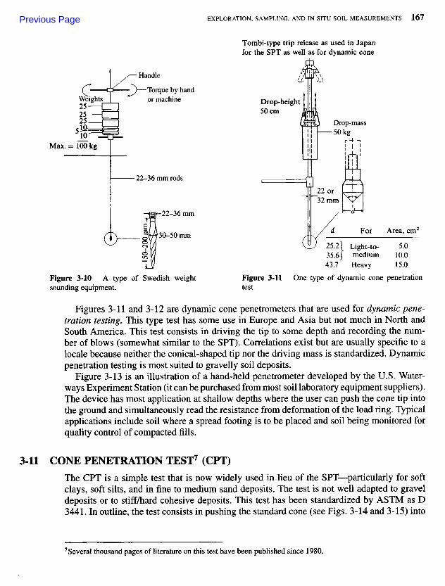
Figure 3-10 A type of Swedish weight Figure 3-11 One type of dynamic cone penetrationsounding equipment. test.
Figures 3-11 and 3-12 are dynamic cone penetrometers that are used for dynamic pene-tration testing. This type test has some use in Europe and Asia but not much in North andSouth America. This test consists in driving the tip to some depth and recording the num-ber of blows (somewhat similar to the SPT). Correlations exist but are usually specific to alocale because neither the conical-shaped tip nor the driving mass is standardized. Dynamicpenetration testing is most suited to gravelly soil deposits.
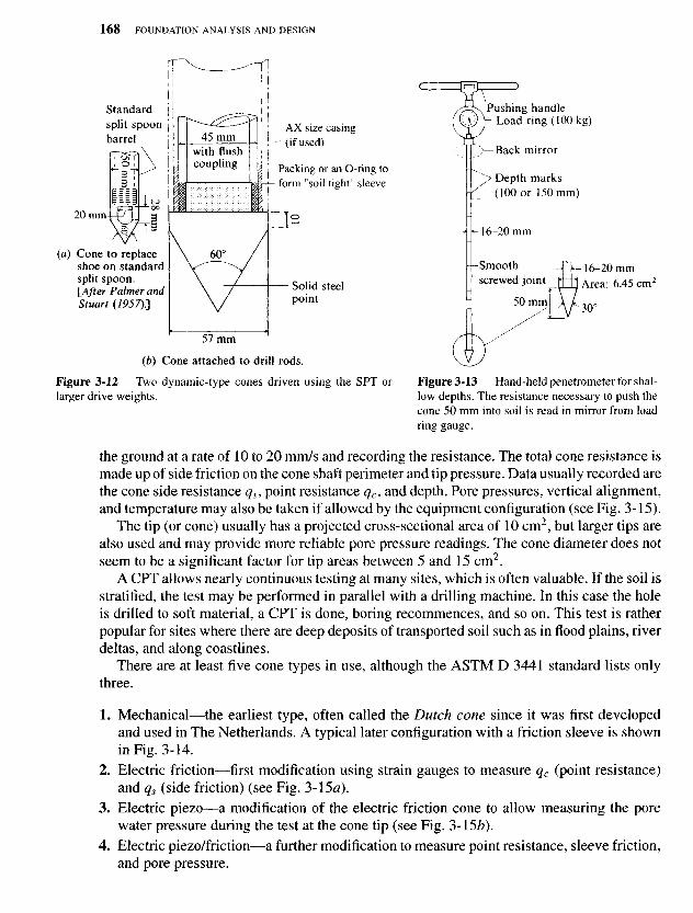
Figure 3-13 is an illustration of a hand-held penetrometer developed by the U.S. Water-ways Experiment Station (it can be purchased from most soil laboratory equipment suppliers).The device has most application at shallow depths where the user can push the cone tip intothe ground and simultaneously read the resistance from deformation of the load ring. Typicalapplications include soil where a spread footing is to be placed and soil being monitored forquality control of compacted fills.
3-11 CONE PENETRATION TEST7 (CPT)
The CPT is a simple test that is now widely used in lieu of the SPT—particularly for softclays, soft silts, and in fine to medium sand deposits. The test is not well adapted to graveldeposits or to stiff/hard cohesive deposits. This test has been standardized by ASTM as D3441. In outline, the test consists in pushing the standard cone (see Figs. 3-14 and 3-15) into
7Several thousand pages of literature on this test have been published since 1980.
Tombi-type trip release as used in Japanfor the SPT as well as for dynamic cone
Handle
Torque by handor machine Drop-height
50 cm
Drop-mass
For Area, cm2
Weights
22-36 mm rods
Light-to-mediumHeavy
Previous Page
Figure 3-13 Hand-held penetrometer for shal-low depths. The resistance necessary to push thecone 50 mm into soil is read in mirror from loadring gauge.
the ground at a rate of 10 to 20 mm/s and recording the resistance. The total cone resistance ismade up of side friction on the cone shaft perimeter and tip pressure. Data usually recorded arethe cone side resistance qs, point resistance qc, and depth. Pore pressures, vertical alignment,and temperature may also be taken if allowed by the equipment configuration (see Fig. 3-15).
The tip (or cone) usually has a projected cross-sectional area of 10 cm2, but larger tips arealso used and may provide more reliable pore pressure readings. The cone diameter does notseem to be a significant factor for tip areas between 5 and 15 cm2.
A CPT allows nearly continuous testing at many sites, which is often valuable. If the soil isstratified, the test may be performed in parallel with a drilling machine. In this case the holeis drilled to soft material, a CPT is done, boring recommences, and so on. This test is ratherpopular for sites where there are deep deposits of transported soil such as in flood plains, riverdeltas, and along coastlines.
There are at least five cone types in use, although the ASTM D 3441 standard lists onlythree.
1. Mechanical—the earliest type, often called the Dutch cone since it was first developedand used in The Netherlands. A typical later configuration with a friction sleeve is shownin Fig. 3-14.
2. Electric friction—first modification using strain gauges to measure qc (point resistance)and qs (side friction) (see Fig. 3-15«).
3. Electric piezo—a modification of the electric friction cone to allow measuring the porewater pressure during the test at the cone tip (see Fig. 3-15&).
4. Electric piezo/friction—a further modification to measure point resistance, sleeve friction,and pore pressure.
(b) Cone attached to drill rods.
Figure 3-12 Two dynamic-type cones driven using the SPT orlarger drive weights.
Solid steelpoint
(a) Cone to replaceshoe on standardsplit spoon.[After Palmer andStuart (7957).]
Standardsplit spoonbarrel
AX size casing(if used)
Packing or an O-ring toform "soil tight" sleeve
Pushing handleLoad ring (100 kg)
Back mirror
Depth marks(100 or 150 mm)
Smoothscrewed joint
with flushcoupling
Area:
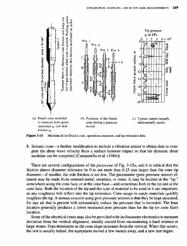
Figure 3-14 Mechanical (or Dutch) cone, operations sequence, and tip resistance data.
5. Seismic cone—a further modification to include a vibration sensor to obtain data to com-pute the shear wave velocity from a surface hammer impact so that the dynamic shearmodulus can be computed [Campanella et al. (1986)].
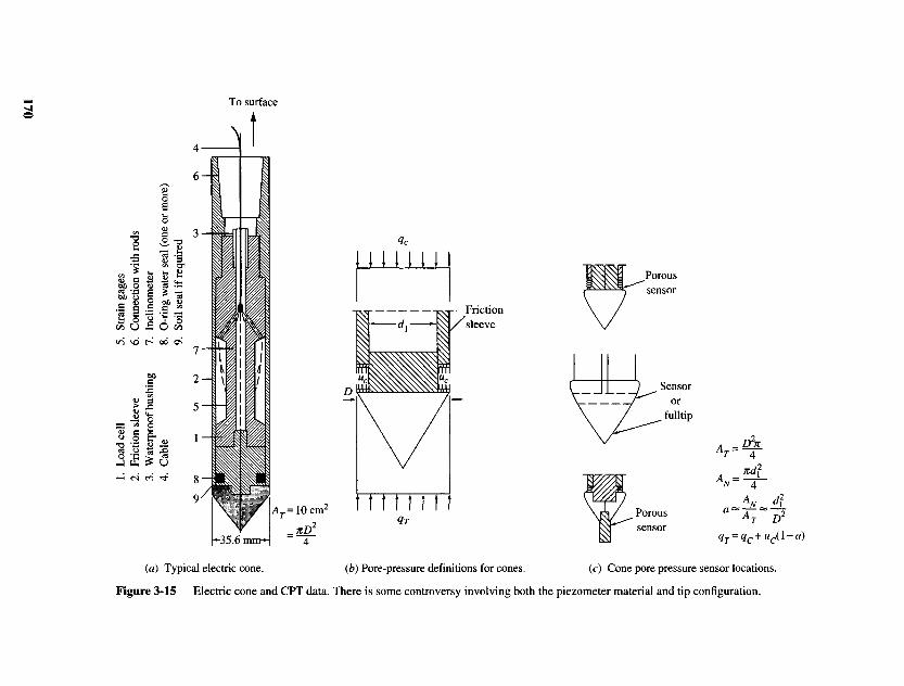
There are several configurations of the piezocone of Fig. 3-15a, and it is critical that thefriction sleeve diameter tolerance be 0 to not more than 0.25 mm larger than the cone tipdiameter—if smaller, the side friction is too low. The piezometer (pore pressure sensor) el-ement may be made from sintered metal, ceramics, or stone. It may be located at the "tip,"somewhere along the cone face, or at the cone base—and sometimes both in the tip and at thecone base. Both the location of the tip and the type of material to be used in it are important,as any roughness will reflect into the tip resistance. Cone usage in sandy materials quicklyroughens the tip. A serious concern using pore pressure sensors is that they be kept saturated,for any air that is present will substantially reduce the pressure that is recorded. The baselocation generally produces a lower measured pore pressure than for the tip (or cone face)location.
Some of the electrical cones may also be provided with inclinometer electronics to measuredeviation from the vertical alignment, usually caused from encountering a hard stratum orlarge stones. Data deteriorate as the cone slope increases from the vertical. When this occurs,the test is usually halted, the equipment moved a few meters away, and a new test begun.
(b) Positions of the Dutchcone during a pressurerecord.
(c) Typical output (usuallyelectronically made).
(a) Dutch cone modifiedto measure both pointresistance qc and skinfriction qf.
Loo
se s
and
Silt
ysa
ndSt
iff c
lay
Sand
Tip pressureqc in kPa
Tap
ered
sle
eve
to e
lim
inat
e co
ne f
rict
ion
and
keep
soi
lou
t of
gap
for
med
whe
n co
ne i
s pu
shed
. P
ushi
ng ja
cket
sepa
rate
ly m
easu
res
skin
fri
ctio
n de
velo
ped
on j
acke
t.
Dep
th b
elow
gro
und
surf
ace,
m
Jack
et
60°
cone
with
3.5
6-cm
bas
e di
amet
er.
Are
a =
10
cm2
Pos. 1Pos. 2
Pos. 3 Pos. 4
(a) Typical electric cone. (b) Pore-pressure definitions for cones. (c) Cone pore pressure sensor locations.
Figure 3-15 Electric cone and CPT data. There is some controversy involving both the piezometer material and tip configuration.
To surface
Poroussensor
Sensoror
fulltip
Poroussensor
Frictionsleeve
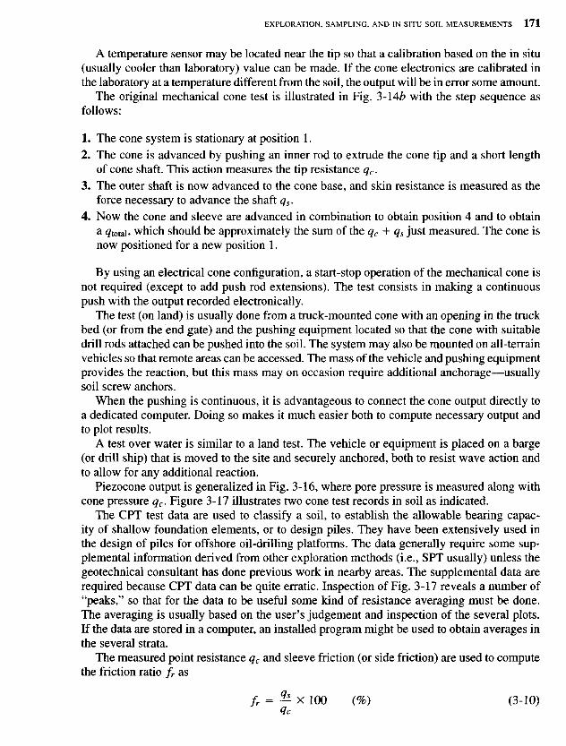
A temperature sensor may be located near the tip so that a calibration based on the in situ(usually cooler than laboratory) value can be made. If the cone electronics are calibrated inthe laboratory at a temperature different from the soil, the output will be in error some amount.
The original mechanical cone test is illustrated in Fig. 3-14Z? with the step sequence asfollows:
1. The cone system is stationary at position 1.2. The cone is advanced by pushing an inner rod to extrude the cone tip and a short length
of cone shaft. This action measures the tip resistance qc.3. The outer shaft is now advanced to the cone base, and skin resistance is measured as the
force necessary to advance the shaft qs.4. Now the cone and sleeve are advanced in combination to obtain position 4 and to obtain
a <?totah which should be approximately the sum of the qc + qs just measured. The cone isnow positioned for a new position 1.
By using an electrical cone configuration, a start-stop operation of the mechanical cone isnot required (except to add push rod extensions). The test consists in making a continuouspush with the output recorded electronically.
The test (on land) is usually done from a truck-mounted cone with an opening in the truckbed (or from the end gate) and the pushing equipment located so that the cone with suitabledrill rods attached can be pushed into the soil. The system may also be mounted on all-terrainvehicles so that remote areas can be accessed. The mass of the vehicle and pushing equipmentprovides the reaction, but this mass may on occasion require additional anchorage—usuallysoil screw anchors.
When the pushing is continuous, it is advantageous to connect the cone output directly toa dedicated computer. Doing so makes it much easier both to compute necessary output andto plot results.
A test over water is similar to a land test. The vehicle or equipment is placed on a barge(or drill ship) that is moved to the site and securely anchored, both to resist wave action andto allow for any additional reaction.
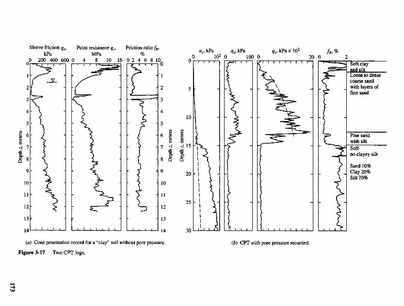
Piezocone output is generalized in Fig. 3-16, where pore pressure is measured along withcone pressure qc. Figure 3-17 illustrates two cone test records in soil as indicated.
The CPT test data are used to classify a soil, to establish the allowable bearing capac-ity of shallow foundation elements, or to design piles. They have been extensively used inthe design of piles for offshore oil-drilling platforms. The data generally require some sup-plemental information derived from other exploration methods (i.e., SPT usually) unless thegeotechnical consultant has done previous work in nearby areas. The supplemental data arerequired because CPT data can be quite erratic. Inspection of Fig. 3-17 reveals a number of"peaks," so that for the data to be useful some kind of resistance averaging must be done.The averaging is usually based on the user's judgement and inspection of the several plots.If the data are stored in a computer, an installed program might be used to obtain averages inthe several strata.
The measured point resistance qc and sleeve friction (or side friction) are used to computethe friction ratio fr as
(3-10)
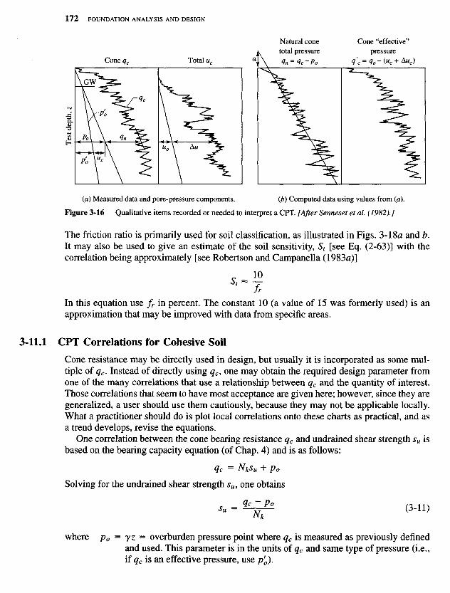
(a) Measured data and pore-pressure components. (b) Computed data using values from (a).
Figure 3-16 Qualitative items recorded or needed to interpret a CPT. [After Senneset et al (1982).]
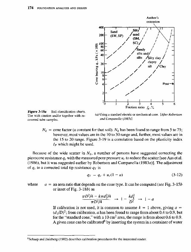
The friction ratio is primarily used for soil classification, as illustrated in Figs. 3- 18a and b.It may also be used to give an estimate of the soil sensitivity, St [see Eq. (2-63)] with thecorrelation being approximately [see Robertson and Campanella (1983a)]
c 1 0
In this equation use fr in percent. The constant 10 (a value of 15 was formerly used) is anapproximation that may be improved with data from specific areas.
3-11.1 CPT Correlations for Cohesive Soil
Cone resistance may be directly used in design, but usually it is incorporated as some mul-tiple of qc. Instead of directly using qc, one may obtain the required design parameter fromone of the many correlations that use a relationship between qc and the quantity of interest.Those correlations that seem to have most acceptance are given here; however, since they aregeneralized, a user should use them cautiously, because they may not be applicable locally.What a practitioner should do is plot local correlations onto these charts as practical, and asa trend develops, revise the equations.
One correlation between the cone bearing resistance qc and undrained shear strength su isbased on the bearing capacity equation (of Chap. 4) and is as follows:
qc = Nksu + Po
Solving for the undrained shear strength su, one obtains
Qc ~ Po n i nSU = -Tj (3-H)
where po = yz — overburden pressure point where qc is measured as previously definedand used. This parameter is in the units of qc and same type of pressure (i.e.,if qc is an effective pressure, use p'o).
Tes
t de
pth,
zCone qc Total uc
Natural conetotal pressure
Cone "effective"pressure
(a) Cone penetration record for a "clay" soil without pore pressure. (b) CPT with pore pressure recorded.
Figure 3-17 Two CPT logs.
Friction ratio fR,%
Point resistance qc,MPa
Sleeve friction qs,kPa
30T x M* «b*&"*B<pi iO
n %*S
Fine sandwith siltSoftno clayey silt
%0Z ^D%0t PireS
Loose to densecoarse sandwith layers offine sand
Soft clayand silt
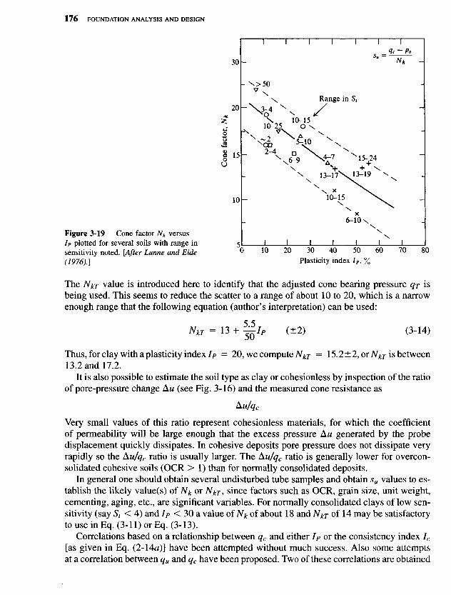
Nk = cone factor (a constant for that soil). Nk has been found to range from 5 to 75;however, most values are in the 10 to 30 range and, further, most values are inthe 15 to 20 range. Figure 3-19 is a correlation based on the plasticity indexIp which might be used.
Because of the wide scatter in Nk, a number of persons have suggested correcting thepiezocone resistance qc with the measured pore pressure uc to reduce the scatter [see Aas et al.(1986), but it was suggested earlier by Robertson and Campanella (1983a)]. The adjustmentof qc to a corrected total tip resistance qj is
qr = qc + uc(l-a) (3-12)
where a = an area ratio that depends on the cone type. It can be computed (see Fig. 3-l5bor inset of Fig. 3-18Z?) as
TTD1IA - kirdi/A _ kd\
~T~T~WA ' W -*
If calibration is not used, it is common to assume k = 1 above, giving a =(d\/D)2\ from calibration, a has been found to range from about 0.4 to 0.9, butfor the "standard cone," with a 10 cm2 area, the range is from about 0.6 to 0.9.A given cone can be calibrated8 by inserting the system in a container of water
8Schaap and Zuidberg (1982) describes calibration procedures for the interested reader.
Figure 3-18a Soil classification charts.Use with caution and/or together with re-covered tube samples.
Friction ratio fR, %
(a) Using a standard electric or mechanical cone. [After Robertsonand Campanella (1983).]
Con
e be
arin
g q c
, k
Pa
( x
100)
Author'sextension
Sand(SW, SP)
Siltysand(SM,SC)
Sandysilts and,silts Silty clay
clayeysilt Clay
Peat
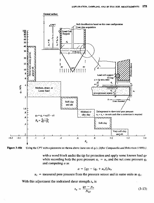
Figure 3-1Sb Using the CPT with a piezocone as shown above (note use of qT). [After Campanella and Robertson (1988). J.
with a wood block under the tip for protection and apply some known load qrwhile recording both the pore pressure uc = uo and the net cone pressure qc
and computing a as
a = [qT ~ (qc + uo)]/uo
uc = measured pore pressure from the pressure sensor and in same units as qc.
With this adjustment the undrained shear strength su is
q T,
MPa
Den
se s
and,
san
dy g
rave
l,gl
acia
l ti
ll
Fric
tion
slee
ve
(3-13)
Bo
Medium, dense, orLoose Sand
Stiff clayand silt
Medium orsilty clay
Enlargement to show total pore pressureuc= uo+ Au acts such that a correction is required
Soft clay
Very soft clayand, silt
(cone diameter)
pore- pressure .sensoj
Load cell supportO-ring
a = tip area ratio
Ground surface
Soil classification based on this cone configurationCone data acquisition
Load CellSupport
Figure 3-19 Cone factor Nk versusIP plotted for several soils with range insensitivity noted. [After Lunne and Eide(1976).]
The NkT value is introduced here to identify that the adjusted cone bearing pressure qj isbeing used. This seems to reduce the scatter to a range of about 10 to 20, which is a narrowenough range that the following equation (author's interpretation) can be used:
NkT = 13 + J^IP (±2) (3-14)
Thus, for clay with a plasticity index//> = 20, we compute NkT = 15.2 ±2, or NkT is between13.2 and 17.2.
It is also possible to estimate the soil type as clay or cohesionless by inspection of the ratioof pore-pressure change Aw (see Fig. 3-16) and the measured cone resistance as
ku/qc
Very small values of this ratio represent cohesionless materials, for which the coefficientof permeability will be large enough that the excess pressure Aw generated by the probedisplacement quickly dissipates. In cohesive deposits pore pressure does not dissipate veryrapidly so the Aw/#c ratio is usually larger. The Aw/#c ratio is generally lower for overcon-solidated cohesive soils (OCR > 1) than for normally consolidated deposits.
In general one should obtain several undisturbed tube samples and obtain su values to es-tablish the likely value(s) of Nk or NkT, since factors such as OCR, grain size, unit weight,cementing, aging, etc., are significant variables. For normally consolidated clays of low sen-sitivity (say S, < 4) and Ip < 30 a value of Nk of about 18 and NkT of 14 may be satisfactoryto use in Eq. (3-11) or Eq. (3-13).
Correlations based on a relationship between qc and either IP or the consistency index Ic
[as given in Eq. (2-14a)] have been attempted without much success. Also some attemptsat a correlation between qu and qc have been proposed. Two of these correlations are obtained
Plasticity index /P , %
Con
e fa
ctor
, JV
*
Range in St
from Sarac and Popovic (1982) as follows:
qc = a + blc
qc = 612.6 + 587.5/c kPa % ^qc = a + bqu
qc = 525.1 + 1.076<?ttkPa
In these equations lc is a decimal quantity, and both qu and qc are in kPa. These two corre-lations can be as much as ±30 percent in error—f or example, if the computed value is 1000kPa, the field value can be anywhere in a range of 700 to 1300 kPa.
Sully et al. (1988) give a correlation for the OCR using a piezocone as shown in Fig. 3-15a with pore pressure sensors installed at the cone base and either on the tip or in the lowerhalf of the cone face. During a test the tip sensor should read a higher pore pressure than thesensor at the cone base. Defining this pore pressure difference as PPD gives us
PPD = fe) -(«] (3-16)W/tip WAase
where uo = in situ static pore pressure ywz in the same units as the pore pressures uc mea-sured at the cone tip and base. A least squares analysis using a number of soils gives
OCR = 0.66 + 1.43 PPD (3-17)
with a correlation coefficient of r — 0.98 (1.0 would be exact). Sully (1988a) revised Eq.(3-17) to
OCR = 0.49 + 1.50 PPD (r = 0.96) (Z-YIa)
Again, on a much larger database, Sully (1990) revised Eq. (3-17) to
OCR = 0.50 + 1.50 PPD (3-17*)
The best range of this equation is for OCR < 10. Equations (3-17) were developed usingpore-pressure data in clays, so they probably should not be used for sands. See Eq. (3-19a)for another equation for OCR applicable for both clay and sand.
3-11.2 CPT Correlations for Cohesionless Soils
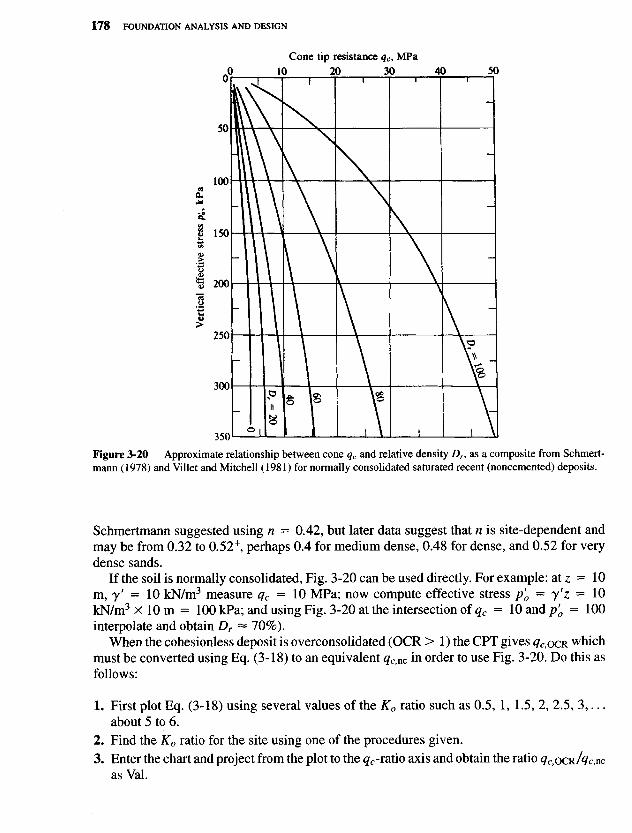
Figure 3-20 is a plot of the correlation between cone pressure qc and relative density Dr. Thisfigure represents the author's composite from references given. The curves are for normallyconsolidated cohesionless material. If the soil is overconsolidated, Dr requires correction ac-cording to Schmertmann (and others). The correction uses the following equations:
1OCR = 1 + fc/^OCR_1\ ( 3 _ l g )
Qc,nc \ KOtnc J
Schmertmann (1978) suggested that the k term in this equation be 0.75, however, in otherlocales a different value may produce a better correlation.
In Eq. (3-18) the K0 ratio might be obtained from Eq. (2-23) rearranged and given here asa reader convenience:
(2-23)
Figure 3-20 Approximate relationship between cone qc and relative density Dr, as a composite from Schmert-mann (1978) and Villet and Mitchell (1981) for normally consolidated saturated recent (noncemented) deposits.
Schmertmann suggested using n = 0.42, but later data suggest that n is site-dependent andmay be from 0.32 to 0.52+, perhaps 0.4 for medium dense, 0.48 for dense, and 0.52 for verydense sands.
If the soil is normally consolidated, Fig. 3-20 can be used directly. For example: at z = 10m ? yf = io kN/m3 measure qc = 10 MPa; now compute effective stress po = y'z = 10kN/m3 X 10 m = 100 kPa; and using Fig. 3-20 at the intersection of qc = 10 and p'o = 100interpolate and obtain Dr ~ 70%).
When the cohesionless deposit is overconsolidated (OCR > 1) the CPT gives qc>ocR whichmust be converted using Eq. (3-18) to an equivalent qc>nc in order to use Fig. 3-20. Do this asfollows:
1. First plot Eq. (3-18) using several values of the K0 ratio such as 0.5, 1, 1.5, 2, 2.5, 3 , . . .about 5 to 6.
2. Find the K0 ratio for the site using one of the procedures given.
3. Enter the chart and project from the plot to the gc-ratio axis and obtain the ratio gc,0CR/#c,ncas VaI.
Ver
tica
l ef
fect
ive
stre
ss p
' o, k
Pa
Cone tip resistance qc, MPa
4. Now solve
^ O C R = V a l
_ ffc,OCRqc,nc ~ w
Use this value of qc,nc as the cone tip resistance term qc and using the computed value ofin-situ po enter Fig. 3-20 and obtain the overconsolidated value of Dr.
5. Save the plot so that you can plot local data on it to see whether a better correlation can beobtained.
When the relative density Dr is estimated, use Table 3-4 or Eq. (3-7) to estimate the angleof internal friction <f>.
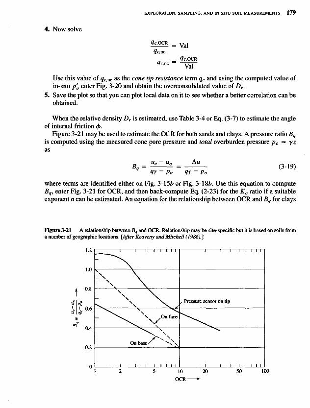
Figure 3-21 may be used to estimate the OCR for both sands and clays. A pressure ratio Bq
is computed using the measured cone pore pressure and total overburden pressure po — yzas
QT ~ Po qr ~ Po
where terms are identified either on Fig. 3-l5b or Fig. 3-lSb. Use this equation to computeBq, enter Fig. 3-21 for OCR, and then back-compute Eq. (2-23) for the K0 ratio if a suitableexponent n can be estimated. An equation for the relationship between OCR and Bq for clays
Figure 3-21 A relationship between Bq and OCR. Relationship may be site-specific but it is based on soils froma number of geographic locations. [After Keaveny and Mitchell (1986).]
OCR
DQ -
Pressure sensor on tip
On face
On base
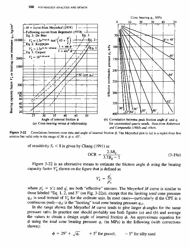
Figure 3-22 Correlations between cone data and angle of internal friction $. The Meyerhof plot in (a) is a replot from fivesources but valid only in the range of 30 ^ <f> < 45°.
of sensitivity St < 8 is given by Chang (1991) as
0 C R - IJB^l < 3- 1 9 a )
Figure 3-22 is an alternative means to estimate the friction angle 0 using the bearingcapacity factor V'b shown on the figure that is defined as
where p'o = y'z and q'c are both "effective" stresses. The Meyerhof M curve is similar tothose labeled "Eq. 1, 2, and 3" (on Fig. 3-22a), except that the limiting total cone pressureqci is used instead of V'b for the ordinate axis. In most cases—particularly if the CPT is acontinuous push—qci is the "limiting" total cone bearing pressure qc\.
In the range shown the Meyerhof M curve tends to give larger (^-angles for the samepressure ratio. In practice one should probably use both figures (a) and (b) and averagethe values to obtain a design angle of internal friction $. An approximate equation for(f> using the total cone bearing pressure qc (in MPa) is the following (with correctionsshown):
<t> = 29° + J^c +5° for gravel; - 5° for silty sand
Angle of internal friction 4>(a) Cone-bearing versus <j> relationship.
(b) Correlation between peak friction angle <f>' and qc
for uncemented quartz sands. Data from Robertsonand Campanella (1983) and others.
Bea
ring
cap
acit
y fa
ctor
V' b
or l
imit
ing
cone
res
ista
nce
q cl,
kg/c
m2
Cone bearing qc, MPa
Eff
ecti
ve o
verb
urde
n pr
essu
re p
' o, k
Pa
M = curve from Meyerhof (1974)Following curves from Begemann (1974)Eq. 3: De Beer
^ ; = 1.3e2*un*tan2(45 + ^ )Eq. 2: Koppejan \ 2J
Eq. 1: Caquot
Mean grain size Z)50, mm
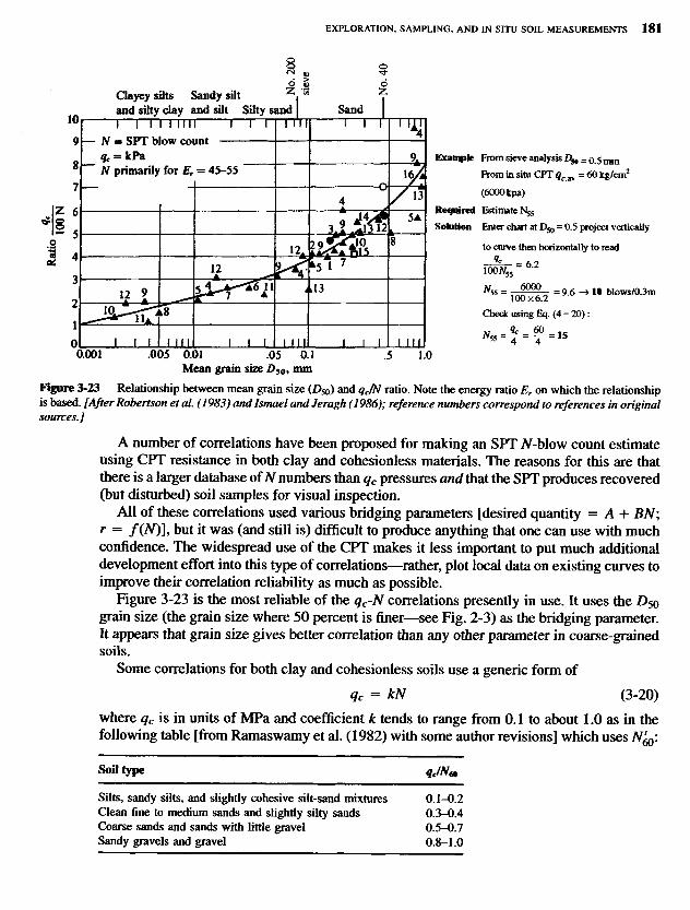
Figure 3-23 Relationship between mean grain size (D50) and qc/N ratio. Note the energy ratio Er on which the relationshipis based. [After Robertson et ah (1983) andlsmael andJeragh (1986); reference numbers correspond to references in originalsources.]
A number of correlations have been proposed for making an SPT TV-blow count estimateusing CPT resistance in both clay and cohesionless materials. The reasons for this are thatthere is a larger database of N numbers than qc pressures and that the SPT produces recovered(but disturbed) soil samples for visual inspection.
All of these correlations used various bridging parameters [desired quantity = A + BN;r = /(N)], but it was (and still is) difficult to produce anything that one can use with muchconfidence. The widespread use of the CPT makes it less important to put much additionaldevelopment effort into this type of correlations—rather, plot local data on existing curves toimprove their correlation reliability as much as possible.
Figure 3-23 is the most reliable of the qc-N correlations presently in use. It uses the D50grain size (the grain size where 50 percent is finer—see Fig. 2-3) as the bridging parameter.It appears that grain size gives better correlation than any other parameter in coarse-grainedsoils.
Some correlations for both clay and cohesionless soils use a generic form of
qc = kN (3-20)
where qc is in units of MPa and coefficient k tends to range from 0.1 to about 1.0 as in thefollowing table [from Ramaswamy et al. (1982) with some author revisions] which uses N^0:
Soil type qc/N<*
Silts, sandy silts, and slightly cohesive silt-sand mixtures 0.1-0.2Clean fine to medium sands and slightly silty sands 0.3-0.4Coarse sands and sands with little gravel 0.5-0.7Sandy gravels and gravel 0.8-1.0
Rat
i°l<§
N
Example From sieve analysis Z)50 = 0.5 mm
From in situ CPT qczv = 60 kg/cm2
(6000 kpa)
Required Estimate N^5
Solution Enter chart at D50 = 0.5 project vertically
to curve then horizontally to read
iofer6-2
#55 = ^ 0 0 ? = 9.6 -> 10 blows/0.3m
Check using Eq. (4 - 20) :
Clayey siltsand silty clay
Sandy siltand silt Silty sand Sand
N = SPT blow count
N primarily for
No.
200
siev
e
No.
40
To illustrate the scatter in qc versus A^0, one study found that a best fit for a fine silty sandwas k = 0.77 [see Denver (1982)]. Comparing this value to the foregoing table, where onemight obtain something between 0.1 and 0.4 (since qc/N^0 > qc/N'm), we can see that therecould be a substantial difference in what the soil is typed as.
Example 3-5.
Given. qc = 300 kg/cm2 at depth z = 8 m in sand, y' = 11.15 kN/m3.
Required. Estimate angle of internal friction </>.
Solution.
p'o = 8 X 11.15 = 89.2 kPa (effective pressure)
qc = V'bp'o (from Fig. 3-22a)
V'b = ^j = 300 X ^ ^ = 330 (98.07 converts kg/cm2 to kPa)
From Fig. 3-22a at V'b = 330, we project to curves and down and obtain $> = 34.5 to 39.5°, say,cf> = 37°. According to Fig. 3-20, qc versus p'o plots into the upper right corner above Dr = 100and since the maximum Dr = 100 we can with Dr = 100 use Fig. 2-2Ab to obtain </> = 42 to 46°,say, <j> = 44°. From Fig. 3-22Z? and qc = 300 X 98.07/1000 = 29.4 MPa, we obtain <j> » 46°.
We could use <fi = 44° (which is high; also, it is somewhat doubtful whether the soil really hasDr = 100). A better estimate might be
4, - ( 3 7 + 43
4 + 4 6 ) = 42°
The author would probably not use over 40°. Question: Could this soil have OCR > 1?////
Example 3-6. Classify the soil on Fig. 3-Ila at the 10- to 12-m depth. Also estimate the undrainedshear strength su if the average y = 19.65 kN/m3 for the entire depth of the CPT. It is known thatthe profile is entirely in cohesive soil.
Solution. Enlarge the figure on a copy machine and estimate qc = 11 MPa at the depth of interestby eye (with this data digitized into a microcomputer we could readily compute the average qc asthe depth increments X qc summed and divided by the depth interval of 2 m).
From qc — 11 MPa = 1 1 000 kPa and //? = 4 percent (from adjacent plot), use Fig. 3-18« andnote the plot into the "silty sand" zone. This zone is evidently stiff from the large qc, so classify as
Soil: stiff, sandy silt (actual soil is a gray, stiff clay, CH)
For s u,
Compute po = y X average depth = 19.65 X 11 = 216 kPa
From Fig. 3-19 estimate Nk = 18 (using our just-made classification for a stiff sandy silt, we wouldexpect an Ip on the order of 10 or less). With this estimate we can use Eq. (3-11) directly to obtain
11000-216w = To = 60OkPa
Io(From laboratory tests su was approximately 725 kPa.)
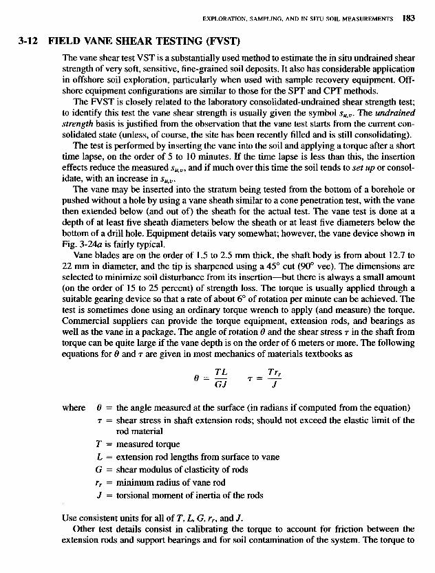
3-12 FIELD VANE SHEAR TESTING (FVST)
The vane shear test VST is a substantially used method to estimate the in situ undrained shearstrength of very soft, sensitive, fine-grained soil deposits. It also has considerable applicationin offshore soil exploration, particularly when used with sample recovery equipment. Off-shore equipment configurations are similar to those for the SPT and CPT methods.
The FVST is closely related to the laboratory consolidated-undrained shear strength test;to identify this test the vane shear strength is usually given the symbol su>v. The undrainedstrength basis is justified from the observation that the vane test starts from the current con-solidated state (unless, of course, the site has been recently filled and is still consolidating).
The test is performed by inserting the vane into the soil and applying a torque after a shorttime lapse, on the order of 5 to 10 minutes. If the time lapse is less than this, the insertioneffects reduce the measured sUfV, and if much over this time the soil tends to set up or consol-idate, with an increase in sUtV.
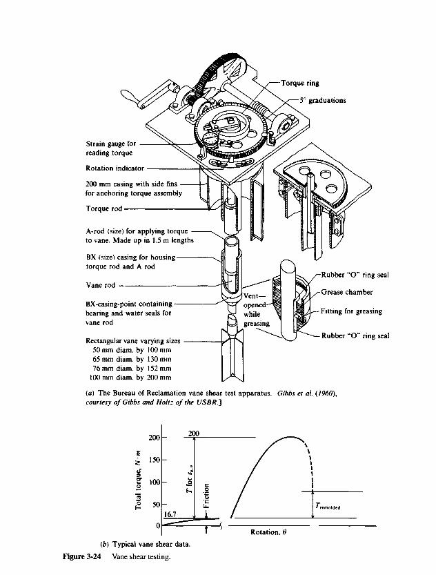
The vane may be inserted into the stratum being tested from the bottom of a borehole orpushed without a hole by using a vane sheath similar to a cone penetration test, with the vanethen extended below (and out of) the sheath for the actual test. The vane test is done at adepth of at least five sheath diameters below the sheath or at least five diameters below thebottom of a drill hole. Equipment details vary somewhat; however, the vane device shown inFig. 3-24a is fairly typical.
Vane blades are on the order of 1.5 to 2.5 mm thick, the shaft body is from about 12.7 to22 mm in diameter, and the tip is sharpened using a 45° cut (90° vee). The dimensions areselected to minimize soil disturbance from its insertion—but there is always a small amount(on the order of 15 to 25 percent) of strength loss. The torque is usually applied through asuitable gearing device so that a rate of about 6° of rotation per minute can be achieved. Thetest is sometimes done using an ordinary torque wrench to apply (and measure) the torque.Commercial suppliers can provide the torque equipment, extension rods, and bearings aswell as the vane in a package. The angle of rotation 0 and the shear stress T in the shaft fromtorque can be quite large if the vane depth is on the order of 6 meters or more. The followingequations for 0 and r are given in most mechanics of materials textbooks as
- i *-?where 0 = the angle measured at the surface (in radians if computed from the equation)
T = shear stress in shaft extension rods; should not exceed the elastic limit of therod material
T = measured torqueL = extension rod lengths from surface to vaneG = shear modulus of elasticity of rodsrr = minimum radius of vane rodJ = torsional moment of inertia of the rods
Use consistent units for all of T, L, G, rr, and J.Other test details consist in calibrating the torque to account for friction between the
extension rods and support bearings and for soil contamination of the system. The torque to
(b) Typical vane shear data.
Figure 3-24 Vane shear testing.
Tot
al t
orqu
e, N
• m
Rotation, 6
(a) The Bureau of Reclamation vane shear test apparatus. Gibbs et al. (I960),courtesy of Gibbs and Holtz of the USBR.]
Rectangular vane varying sizes50 mm diam. by 100 mm65 mm diam. by 130 mm76 mm diam. by 152 mm
100 mm diam. by 200 mm
BX-casing-point containingbearing and water seals forvane rod
Vane rod
BX (size) casing for housingtorque rod and A rod
A-rod (size) for applying torqueto vane. Made up in 1.5 m lengths
Torque rod
200 mm casing with side finsfor anchoring torque assembly
Rotation indicator
Strain gauge forreading torque
Torque ring
5° graduations
Rubber "O" ring seal
Grease chamber
Fitting for greasing
Rubber "O" ring seal
Ventopenedwhilegreasing
Fric
tion
shear the soil around the perimeter is corrected by calibration, as illustrated in Fig. 3-246. It iscommon to continue the vane rotation for 10 to 12 complete revolutions after the peak value(which occurs at soil rupture) so that the soil in the shear zone is substantially remolded. Arest period of 1 to 2 min is taken, then a second torque reading is made to obtain the residual(or remolded) strength. The ratio of these two strengths should be approximately the soilsensitivity St.
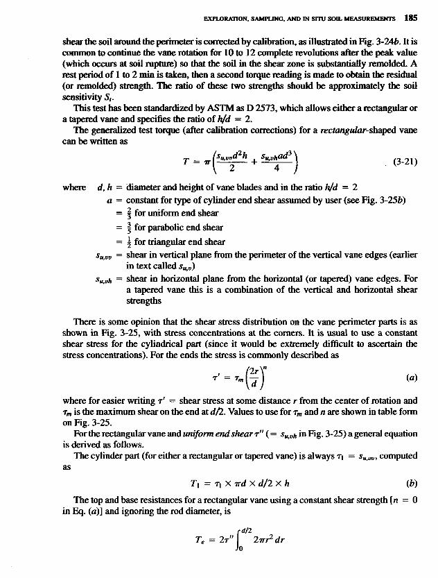
This test has been standardized by ASTM as D 2573, which allows either a rectangular ora tapered vane and specifies the ratio of h/d = 2.
The generalized test torque (after calibration corrections) for a rectangular-shaped vanecan be written as
r / £ ^ + £ ^ \ ( 3 2 1 )
where d, h = diameter and height of vane blades and in the ratio h/d = 2a = constant for type of cylinder end shear assumed by user (see Fig. 3-256)
= \ for uniform end shear= \ for parabolic end shear= \ for triangular end shear
Su9UU = shear in vertical plane from the perimeter of the vertical vane edges (earlierin text called sU)V)
su,vh = shear in horizontal plane from the horizontal (or tapered) vane edges. Fora tapered vane this is a combination of the vertical and horizontal shearstrengths
There is some opinion that the shear stress distribution on the vane perimeter parts is asshown in Fig. 3-25, with stress concentrations at the corners. It is usual to use a constantshear stress for the cylindrical part (since it would be extremely difficult to ascertain thestress concentrations). For the ends the stress is commonly described as
" - ^ ywhere for easier writing T' = shear stress at some distance r from the center of rotation andrm is the maximum shear on the end at d/2. Values to use for rm and n are shown in table formon Fig. 3-25.
For the rectangular vane and uniform end shear T" ( = sUfVh in Fig. 3-25) a general equationis derived as follows.
The cylinder part (for either a rectangular or tapered vane) is always T\ = sUfVV, computedas
T1 = n X ird X d/2 X h (Jb)
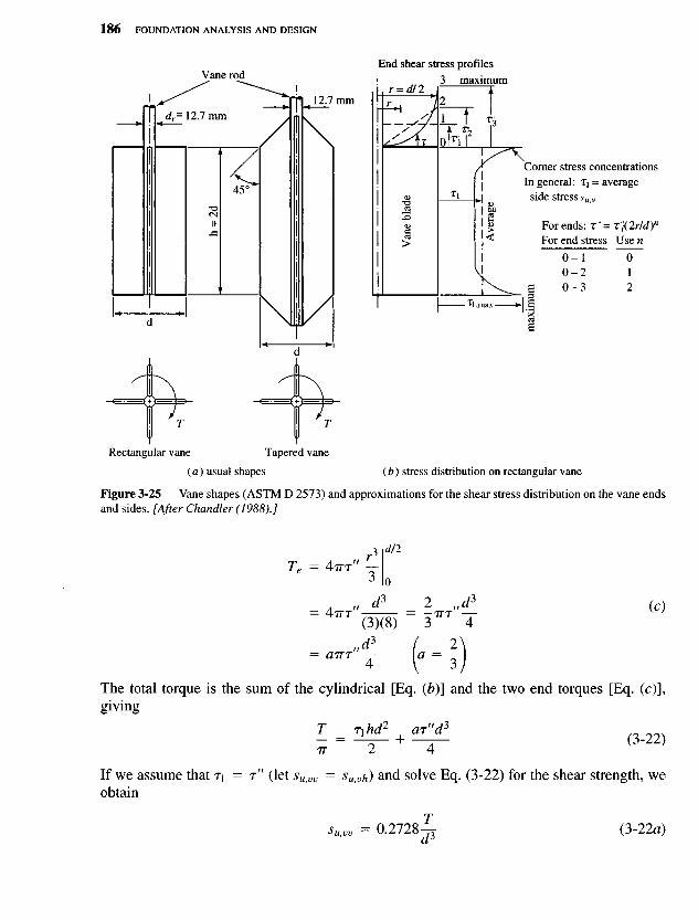
The top and base resistances for a rectangular vane using a constant shear strength [n = 0in Eq. (a)] and ignoring the rod diameter, is
Rectangular vane Tapered vane
(a) usual shapes (b) stress distribution on rectangular vane
Figure 3-25 Vane shapes (ASTM D 2573) and approximations for the shear stress distribution on the vane endsand sides. [After Chandler (1988).]
Te = 47TT" V-5 0
(3)(8) 3 4
= a™ T (a = 3 jThe total torque is the sum of the cylindrical [Eq. (b)] and the two end torques [Eq. (c)],giving
T ^ M + ar^TT 2 4
If we assume that Ti = r" (let sUtVV = su>vh) and solve Eq. (3-22) for the shear strength, weobtain
Vane rodEnd shear stress profiles
maximum
Corner stress concentrationsIn general: Ti = average
side stress s u>v
Van
e bl
ade
Ave
rage
For ends: T" = T11XIrIdYFor end stress Usen
0 - 10-20-3
012
max
imum
(3-22a)
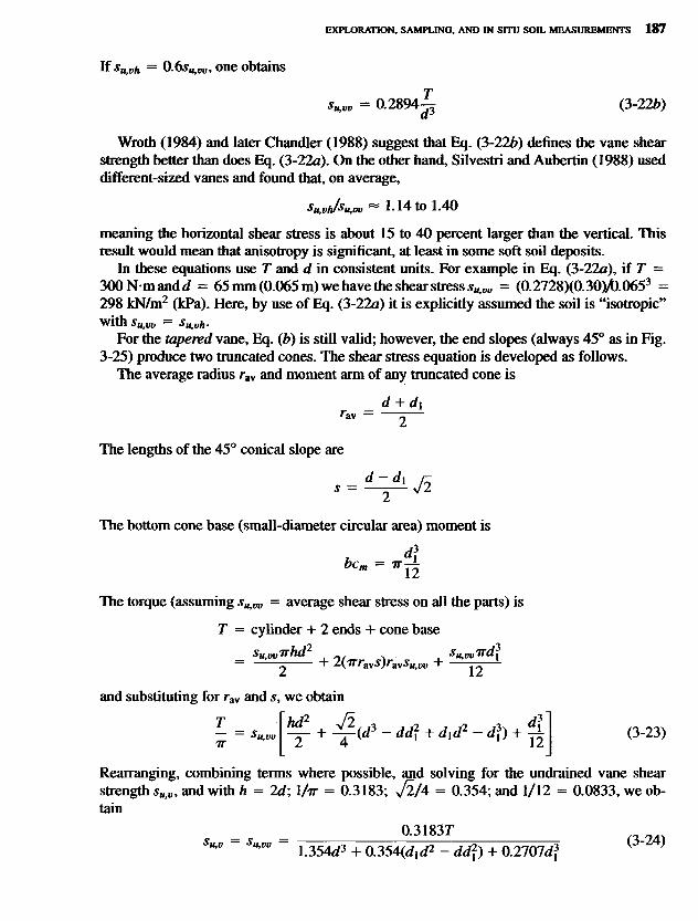
If^uA = 0.65^170, one obtains
SutUV = 0.2894 J Q-22b)
Wroth (1984) and later Chandler (1988) suggest that Eq. (3-226) defines the vane shearstrength better than does Eq. (3-22a). On the other hand, Silvestri and Aubertin (1988) useddifferent-sized vanes and found that, on average,
Su,vh/su,w ~ 1.14 to 1.40
meaning the horizontal shear stress is about 15 to 40 percent larger than the vertical. Thisresult would mean that anisotropy is significant, at least in some soft soil deposits.
In these equations use T and d in consistent units. For example in Eq. (3-22a), if T =300 N m and d = 65 mm (0.065 m) we have the shear stress su,vv = (0.2728)(0.30)/3.0653 =298 kN/m2 (kPa). Here, by use of Eq. (3-22a) it is explicitly assumed the soil is "isotropic"W l u l ISI UU SjiyVh*
For the tapered vane, Eq. (b) is still valid; however, the end slopes (always 45° as in Fig.3-25) produce two truncated cones. The shear stress equation is developed as follows.
The average radius rav and moment arm of any truncated cone is
_ d + J1
The lengths of the 45° conical slope are
The bottom cone base (small-diameter circular area) moment is
bcm = TTjt
The torque (assuming sUrVV = average shear stress on all the parts) is
T = cylinder + 2 ends + cone base
_ ^ M 2 su,vv<nd\
and substituting for rav and s, we obtain
- = S11J^ + - dd\ + J1J2 - d\) + ] (3-23)
Rearranging, combining terms where possible, and solving for the undrained vane shearstrength sUiV, and with h = 2d; l/ir = 0.3183; Jl/A = 0.354; and 1/12 = 0.0833, we ob-tain
(3-24)
where in all these equations d = vane diameterd\ = shaft diameter at vane, usually about 12 to 22 mm. Equa-
tion (3-24) is greatly simplified if the dd\ terms are ne-glected.
T = measured torque
Use consistent units of T in N-m with d in m, or T in N-mm with d in mm. Use kN insteadof N if numbers become very large.
Somewhat similar to the SPT, the vane test is usually performed every 0.5 to 1 m of depth insoft clays and fine silty sands. The test is not well suited for dense, hard, or gravelly deposits.
The generic forms of Eq. (3-24) allow the user to perform two tests in the stratum usingdifferent vane dimensions to obtain estimates of both sUiVV and su>vh. This is seldom done,however, and either the soil is assumed isotropic or the horizontal shear strength sUtVh is somefraction (say, 0.5, 0.6, etc.) of the vertical strength sUtVV.
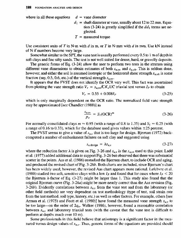
It appears that the FVST does not identify the OCR very well. This fact was ascertainedfrom plotting the vane strength ratio Vr = sUfVV/CKoUC triaxial test versus Ip to obtain
Vr = 0.55 + 0.008/p (3-25)
which is only marginally dependent on the OCR ratio. The normalized field vane strengthmay be approximated [see Chandler (1988)] as
^ = Si(OCR)"1 (3-26)Po
For normally consolidated clays m « 0.95 (with a range of 0.8 to 1.35) and S\ ~ 0.25 (witha range of 0.16 to 0.33), which for the database used gives values within ±25 percent.
The FVST seems to give a value of sUtV that is too large for design. Bjerrum (1972) back-computed a number of embankment failures on soft clay and suggested using
^M,design = "-Suv (J-Z/)
where the reduction factor A is given on Fig. 3-26 and sUtV is the sUtVV used to this point. Laddet al. (1977) added additional data to support Fig. 3-26 but observed that there was substantialscatter in the points. Aas et al. (1986) restudied the Bjerrum chart, to include OCR and aging,and produced the revised chart of Fig. 3-26fc. Both charts are included, since Bjerrum's charthas been widely used; however, the revised Aas chart appears more rational. Lefebvre et al.(1988) studied two soft, sensitive clays with a low Ip and found that for cases where Ip < 20the Bjerrum A-factor of Eq. (3-27) might be larger than 1. This study also found that theoriginal Bjerrum curve (Fig. 3-26a) might be more nearly correct than the Aas revision (Fig.3-26b). Evidently correlations between su>v from the vane test and from the laboratory (orother field methods) are very dependent on test methodology (type of test, soil strain ratefrom the test method, soil type, history, etc.) as well as other factors. For example, others [seeArman et al. (1975) and Foott et al. (1980)] have found the measured vane strength sUfV tobe too large—on the order of 2qu. Walker (1986), however, found a reasonable correlationbetween sUtV and laboratory triaxial tests (with the caveat that the vane test is difficult toperform at depths much over 10m).
Some professionals in this field believe that anisotropy is a significant factor in the mea-sured versus design values of sUtV. Thus, generic forms of the equations are provided should
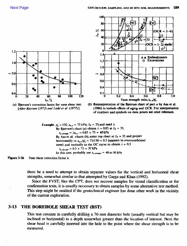
Example: p'o = 150; s..., = 75 kPa; Ir = 35;and need LBy BjerrunVs chart (a) obtain ). = 0.85 at / r = 35.
V d * = ^ * . = 0.85 x 75 = 65kPaBy Aas et al. charts (b\ enter top chart at IP = 35 and projecthorizontally to su%jp'm = 75/150 = 0.5 (appears in overconsolidatedzone) and vertically to the OC curve to obtain A = 0.5
V d e , * n = 0 . 5 x 7 5 = 37kPaIn this case, probably use sB.desifB = 40 to 50 kPa.
Figure 3-26 Vane shear correction factor A.
there be a need to attempt to obtain separate values for the vertical and horizontal shearstrengths, somewhat similar to that attempted by Garga and Khan (1992).
Since the FVST, like the CPT, does not recover samples for visual classification or forconfirmation tests, it is usually necessary to obtain samples by some alternative test method.This step might be omitted if the geotechnical engineer has done other work in the vicinityof the current exploration.
3-13 THEBOREHOLESHEARTEST(BST)
This test consists in carefully drilling a 76-mm diameter hole (usually vertical but may beinclined or horizontal) to a depth somewhat greater than the location of interest. Next theshear head is carefully inserted into the hole to the point where the shear strength is to bemeasured.
(a) Bjerrum's correction factor for vane shear test.[After Bjerrum (1972) and Ladd et al. (1977).]
Vane strength ratio, Sn^Jp'9
(b) Reinterpretation of the Bjerrum chart of part a by Aas et al.(1986) to include effects of aging and OCR. For interpretationof numbers and symbols on data points see cited reference.