4/11/2011 1 Window-based models for generic object detection Monday, April 11 Kristen Grauman UT-Austin Previously • Instance recognition – Local features: detection and description – Local feature matching, scalable indexing – Spatial verification • Intro to generic object recognition • Supervised classification – Main idea – Skin color detection example Last time: supervised classification Feature value x Optimal classifier will minimize total risk. At decision boundary, either choice of label yields same expected loss. So, best decision boundary is at point x where To classify a new point, choose class with lowest expected loss; i.e., choose “four” if 9) (4 ) | 4 is P(class 4) (9 ) | 9 is class ( L L P x x ) 4 9 ( ) | 9 ( ) 9 4 ( ) | 4 ( L P L P x x P(4 | x) P(9 | x) Kristen Grauman Last time: Example: skin color classification • We can represent a class-conditional density using a histogram (a “non-parametric” distribution) Feature x = Hue Feature x = Hue P(x|skin) P(x|not skin) Kristen Grauman • We can represent a class-conditional density using a histogram (a “non-parametric” distribution) Feature x = Hue P(x|skin) Feature x = Hue P(x|not skin) Now we get a new image, and want to label each pixel as skin or non-skin. ) ( ) | ( ) | ( skin P skin x P x skin P Last time: Example: skin color classification Kristen Grauman Now for every pixel in a new image, we can estimate probability that it is generated by skin. Classify pixels based on these probabilities Brighter pixels higher probability of being skin Last time: Example: skin color classification Kristen Grauman
Transcript
4/11/2011
1
Window-based models forgeneric object detection
Monday, April 11
Kristen Grauman
UT-Austin
Previously
• Instance recognition– Local features: detection and description– Local feature matching, scalable indexing– Spatial verification
• Intro to generic object recognition• Supervised classification
– Main idea– Skin color detection example
Last time: supervised classification
Feature value x
Optimal classifier will minimize total risk.
At decision boundary, either choice of label yields same expected loss.
So, best decision boundary is at point x where
To classify a new point, choose class with lowest expected loss; i.e., choose “four” if
9)(4) |4 is P(class4)(9 )|9 is class( LLP xx
)49()|9()94()|4( LPLP xx
P(4 | x) P(9 | x)
Kristen Grauman
Last time: Example: skin color classification
• We can represent a class-conditional density using a histogram (a “non-parametric” distribution)
Feature x = Hue
Feature x = Hue
P(x|skin)
P(x|not skin)
Kristen Grauman
• We can represent a class-conditional density using a histogram (a “non-parametric” distribution)
Feature x = Hue
P(x|skin)
Feature x = Hue
P(x|not skin)Now we get a new image, and want to label each pixel as skin or non-skin.
)()|( )|( skinPskinxPxskinP
Last time: Example: skin color classification
Kristen Grauman
Now for every pixel in a new image, we can estimate probability that it is generated by skin.
• Pixel-based representations sensitive to small shifts
• Color or grayscale-based appearance description can be sensitive to illumination and intra-class appearance variation
Kristen Grauman
Window-based modelsBuilding an object model
• Consider edges, contours, and (oriented) intensity gradients
Kristen Grauman
4/11/2011
3
Window-based modelsBuilding an object model
• Consider edges, contours, and (oriented) intensity gradients
• Summarize local distribution of gradients with histogram Locally orderless: offers invariance to small shifts and rotations Contrast-normalization: try to correct for variable illumination
Kristen Grauman
Window-based modelsBuilding an object model
Car/non-car Classifier
Yes, car.No, not a car.
Given the representation, train a binary classifier
Kristen Grauman
Discriminative classifier construction
106 examples
Nearest neighbor
Shakhnarovich, Viola, Darrell 2003Berg, Berg, Malik 2005...
Viola, Jones 2001, Torralba et al. 2004, Opelt et al. 2006,…
Boosting intuition
Weak Classifier 1
Slide credit: Paul Viola
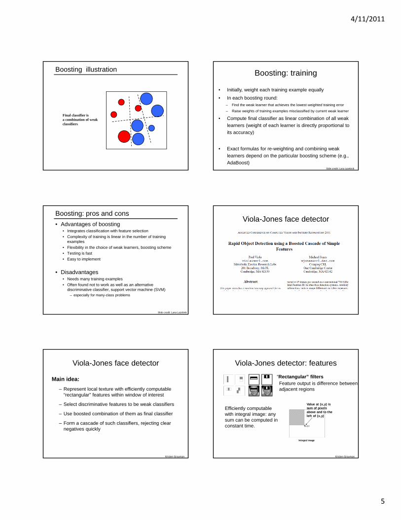
Boosting illustration
WeightsIncreased
Boosting illustration
Weak Classifier 2
Boosting illustration
WeightsIncreased
Boosting illustration
Weak Classifier 3
4/11/2011
5
Boosting illustration
Final classifier is a combination of weak classifiers
Boosting: training
• Initially, weight each training example equally
• In each boosting round:– Find the weak learner that achieves the lowest weighted training error
– Raise weights of training examples misclassified by current weak learner
• Compute final classifier as linear combination of all weak
learners (weight of each learner is directly proportional to
its accuracy)
• Exact formulas for re-weighting and combining weak
learners depend on the particular boosting scheme (e.g.,
AdaBoost)Slide credit: Lana Lazebnik
Boosting: pros and cons
• Advantages of boosting• Integrates classification with feature selection
• Complexity of training is linear in the number of training examples
• Flexibility in the choice of weak learners, boosting scheme
• Testing is fast
• Easy to implement
• Disadvantages• Needs many training examples
• Often found not to work as well as an alternative discriminative classifier, support vector machine (SVM)
– especially for many-class problems
Slide credit: Lana Lazebnik
Viola-Jones face detector
Main idea:
– Represent local texture with efficiently computable “rectangular” features within window of interest
– Select discriminative features to be weak classifiers
– Use boosted combination of them as final classifier
– Form a cascade of such classifiers, rejecting clear negatives quickly
Viola-Jones face detector
Kristen Grauman
Viola-Jones detector: features
Feature output is difference between adjacent regions
Efficiently computable with integral image: any sum can be computed in constant time.
“Rectangular” filters
Value at (x,y) is sum of pixels above and to the left of (x,y)
Integral image
Kristen Grauman
4/11/2011
6
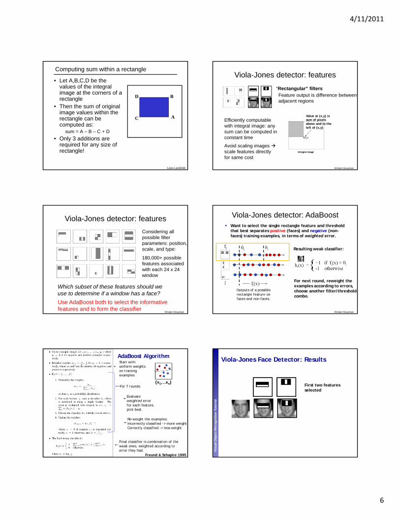
Computing sum within a rectangle
• Let A,B,C,D be the values of the integral image at the corners of a rectangle
• Then the sum of original image values within the rectangle can be computed as:
sum = A – B – C + D
• Only 3 additions are required for any size of rectangle!
D B
C A
Lana Lazebnik
Viola-Jones detector: features
Feature output is difference between adjacent regions
Efficiently computable with integral image: any sum can be computed in constant time
Avoid scaling images scale features directly for same cost
“Rectangular” filters
Value at (x,y) is sum of pixels above and to the left of (x,y)
Integral image
Kristen Grauman
Considering all possible filter parameters: position, scale, and type:
180,000+ possible features associated with each 24 x 24 window
Which subset of these features should we use to determine if a window has a face?
Use AdaBoost both to select the informative features and to form the classifier
Viola-Jones detector: features
Kristen Grauman
Viola-Jones detector: AdaBoost• Want to select the single rectangle feature and threshold
that best separates positive (faces) and negative (non-faces) training examples, in terms of weighted error.
Outputs of a possible rectangle feature on faces and non-faces.
…
Resulting weak classifier:
For next round, reweight the examples according to errors, choose another filter/threshold combo.
Kristen Grauman
Perc
eptu
al a
nd S
enso
ry A
ugm
ente
d C
omputi
ng
Vis
ua
l Ob
jec
t R
ec
og
nit
ion
Tu
tori
al
Vis
ua
l Ob
jec
t R
ec
og
nit
ion
Tu
tori
al
AdaBoost AlgorithmStart with uniform weights on training examples
Evaluate weighted error for each feature, pick best.
Re-weight the examples:Incorrectly classified -> more weightCorrectly classified -> less weight
Final classifier is combination of the weak ones, weighted according to error they had.
Freund & Schapire 1995
{x1,…xn}For T rounds
Perc
eptu
al a
nd S
enso
ry A
ugm
ente
d C
omputi
ng
Vis
ua
l Ob
jec
t R
ec
og
nit
ion
Tu
tori
al
Vis
ua
l Ob
jec
t R
ec
og
nit
ion
Tu
tori
al
First two features selected
Viola-Jones Face Detector: Results
4/11/2011
7
• Even if the filters are fast to compute, each new image has a lot of possible windows to search.
• How to make the detection more efficient?
Cascading classifiers for detection
• Form a cascade with low false negative rates early on
• Apply less accurate but faster classifiers first to immediately discard windows that clearly appear to be negative
Kristen Grauman
Viola-Jones detector: summary
Train with 5K positives, 350M negativesReal‐time detector using 38 layer cascade6061 features in all layers
[Implementation available in OpenCV: http://www.intel.com/technology/computing/opencv/]
Faces
Non-faces
Train cascade of classifiers with
AdaBoost
Selected features, thresholds, and weights
New image
Kristen Grauman
Viola-Jones detector: summary
• A seminal approach to real-time object detection
• Training is slow, but detection is very fast
• Key ideas
Integral images for fast feature evaluation
Boosting for feature selection
Attentional cascade of classifiers for fast rejection of non-face windows
P. Viola and M. Jones. Rapid object detection using a boosted cascade of simple features.CVPR 2001.
P. Viola and M. Jones. Robust real-time face detection. IJCV 57(2), 2004.
Perc
eptu
al a
nd S
enso
ry A
ugm
ente
d C
omputi
ng
Vis
ua
l Ob
jec
t R
ec
og
nit
ion
Tu
tori
al
Vis
ua
l Ob
jec
t R
ec
og
nit
ion
Tu
tori
al
Viola-Jones Face Detector: Results
Perc
eptu
al a
nd S
enso
ry A
ugm
ente
d C
omputi
ng
Vis
ua
l Ob
jec
t R
ec
og
nit
ion
Tu
tori
al
Vis
ua
l Ob
jec
t R
ec
og
nit
ion
Tu
tori
al
Viola-Jones Face Detector: Results
4/11/2011
8
Perc
eptu
al a
nd S
enso
ry A
ugm
ente
d C
omputi
ng
Vis
ua
l Ob
jec
t R
ec
og
nit
ion
Tu
tori
al
Vis
ua
l Ob
jec
t R
ec
og
nit
ion
Tu
tori
al
Viola-Jones Face Detector: Results
Perc
eptu
al a
nd S
enso
ry A
ugm
ente
d C
omputi
ng
Vis
ua
l Ob
jec
t R
ec
og
nit
ion
Tu
tori
al
Vis
ua
l Ob
jec
t R
ec
og
nit
ion
Tu
tori
al
Detecting profile faces?
Can we use the same detector?
Perc
eptu
al a
nd S
enso
ry A
ugm
ente
d C
omputi
ng
Vis
ua
l Ob
jec
t R
ec
og
nit
ion
Tu
tori
al
Vis
ua
l Ob
jec
t R
ec
og
nit
ion
Tu
tori
al
Paul Viola, ICCV tutorial
Viola-Jones Face Detector: Results
Everingham, M., Sivic, J. and Zisserman, A."Hello! My name is... Buffy" - Automatic naming of characters in TV video,BMVC 2006. http://www.robots.ox.ac.uk/~vgg/research/nface/index.html
Example using Viola‐Jones detector
Frontal faces detected and then tracked, character names inferred with alignment of script and subtitles.
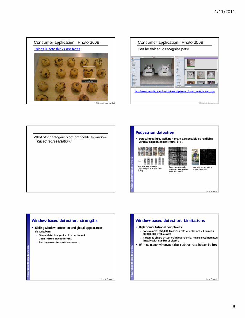
What other categories are amenable to window-based representation?
Perc
eptu
al a
nd S
enso
ry A
ugm
ente
d C
omputi
ng
Vis
ua
l Ob
jec
t R
ec
og
nit
ion
Tu
tori
al
Vis
ua
l Ob
jec
t R
ec
og
nit
ion
Tu
tori
al
Pedestrian detection• Detecting upright, walking humans also possible using sliding
window’s appearance/texture; e.g.,
SVM with Haar wavelets [Papageorgiou & Poggio, IJCV 2000]
Space-time rectangle features [Viola, Jones & Snow, ICCV 2003]
SVM with HoGs [Dalal & Triggs, CVPR 2005]
Kristen Grauman
Perc
eptu
al a
nd S
enso
ry A
ugm
ente
d C
omputi
ng
Vis
ua
l Ob
jec
t R
ec
og
nit
ion
Tu
tori
al
Vis
ua
l Ob
jec
t R
ec
og
nit
ion
Tu
tori
al
Window-based detection: strengths
• Sliding window detection and global appearance descriptors: Simple detection protocol to implement Good feature choices critical Past successes for certain classes
Kristen Grauman
Perc
eptu
al a
nd S
enso
ry A
ugm
ente
d C
omputi
ng
Vis
ua
l Ob
jec
t R
ec
og
nit
ion
Tu
tori
al
Vis
ua
l Ob
jec
t R
ec
og
nit
ion
Tu
tori
al
Window-based detection: Limitations
• High computational complexity For example: 250,000 locations x 30 orientations x 4 scales =
30,000,000 evaluations! If training binary detectors independently, means cost increases
linearly with number of classes
• With so many windows, false positive rate better be low
Kristen Grauman
4/11/2011
10
Perc
eptu
al a
nd S
enso
ry A
ugm
ente
d C
omputi
ng
Vis
ua
l Ob
jec
t R
ec
og
nit
ion
Tu
tori
al
Vis
ua
l Ob
jec
t R
ec
og
nit
ion
Tu
tori
al
Limitations (continued)
• Not all objects are “box” shaped
Kristen Grauman
Perc
eptu
al a
nd S
enso
ry A
ugm
ente
d C
omputi
ng
Vis
ua
l Ob
jec
t R
ec
og
nit
ion
Tu
tori
al
Vis
ua
l Ob
jec
t R
ec
og
nit
ion
Tu
tori
al
Limitations (continued)
• Non-rigid, deformable objects not captured well with representations assuming a fixed 2d structure; or must assume fixed viewpoint
• Objects with less-regular textures not captured well with holistic appearance-based descriptions
Kristen Grauman
Perc
eptu
al a
nd S
enso
ry A
ugm
ente
d C
omputi
ng
Vis
ua
l Ob
jec
t R
ec
og
nit
ion
Tu
tori
al
Vis
ua
l Ob
jec
t R
ec
og
nit
ion
Tu
tori
al
Limitations (continued)
• If considering windows in isolation, context is lost
Figure credit: Derek Hoiem
Sliding window Detector’s view
Kristen Grauman
Perc
eptu
al a
nd S
enso
ry A
ugm
ente
d C
omputi
ng
Vis
ua
l Ob
jec
t R
ec
og
nit
ion
Tu
tori
al
Vis
ua
l Ob
jec
t R
ec
og
nit
ion
Tu
tori
al
Limitations (continued)
• In practice, often entails large, cropped training set (expensive)
• Requiring good match to a global appearance description can lead to sensitivity to partial occlusions
Image credit: Adam, Rivlin, & Shimshoni Kristen Grauman
Summary
• Basic pipeline for window-based detection
– Model/representation/classifier choice
– Sliding window and classifier scoring
• Boosting classifiers: general idea
• Viola-Jones face detector
– Exemplar of basic paradigm
– Plus key ideas: rectangular features, Adaboost for feature selection, cascade
• Pros and cons of window-based detection
� Given example images����������� ����������������������
where����������for negative and positive examples respec-
respec-tively, where ' and ( are the number of negatives andpositives respectively.� For ) �*�+���������-,
:
1. Normalize the weights,
�/. � �10 � . � �2 �3�4 � � . � 3so that �5. is a probability distribution.
2. For each feature, 6 , train a classifier 7 3 whichis restricted to using a single feature. Theerror is evaluated with respect to �8. , 9 3 �2 � � ��: 7 3 ��� � �<;=� �:
.
3. Choose the classifier, 7 . , with the lowest error 9 . .4. Update the weights:
� .�> � � � � � . � �@? � A�B$C.where D �E�F�
if example���
is classified cor-rectly, D � �&�
otherwise, and? . � GIH� A G H .� The final strong classifier is:
where P . �OUWV+X �Y HTable 1: The AdaBoost algorithm for classifier learn-ing. Each round of boosting selects one feature from the180,000 potential features.
number of features are retained (perhaps a few hundred orthousand).
3.2. Learning ResultsWhile details on the training and performance of the finalsystem are presented in Section 5, several simple resultsmerit discussion. Initial experiments demonstrated that afrontal face classifier constructed from 200 features yieldsa detection rate of 95% with a false positive rate of 1 in14084. These results are compelling, but not sufficient formany real-world tasks. In terms of computation, this clas-sifier is probably faster than any other published system,requiring 0.7 seconds to scan an 384 by 288 pixel image.Unfortunately, the most straightforward technique for im-proving detection performance, adding features to the clas-sifier, directly increases computation time.
For the task of face detection, the initial rectangle fea-tures selected by AdaBoost are meaningful and easily inter-preted. The first feature selected seems to focus on the prop-erty that the region of the eyes is often darker than the region
Figure 3: The first and second features selected by Ad-aBoost. The two features are shown in the top row and thenoverlayed on a typical training face in the bottom row. Thefirst feature measures the difference in intensity between theregion of the eyes and a region across the upper cheeks. Thefeature capitalizes on the observation that the eye region isoften darker than the cheeks. The second feature comparesthe intensities in the eye regions to the intensity across thebridge of the nose.
of the nose and cheeks (see Figure 3). This feature is rel-atively large in comparison with the detection sub-window,and should be somewhat insensitive to size and location ofthe face. The second feature selected relies on the propertythat the eyes are darker than the bridge of the nose.
4. The Attentional CascadeThis section describes an algorithm for constructing a cas-cade of classifiers which achieves increased detection per-formance while radically reducing computation time. Thekey insight is that smaller, and therefore more efficient,boosted classifiers can be constructed which reject many ofthe negative sub-windows while detecting almost all posi-tive instances (i.e. the threshold of a boosted classifier canbe adjusted so that the false negative rate is close to zero).Simpler classifiers are used to reject the majority of sub-windows before more complex classifiers are called uponto achieve low false positive rates.
The overall form of the detection process is that of a de-generate decision tree, what we call a “cascade” (see Fig-ure 4). A positive result from the first classifier triggers theevaluation of a second classifier which has also been ad-justed to achieve very high detection rates. A positive resultfrom the second classifier triggers a third classifier, and soon. A negative outcome at any point leads to the immediaterejection of the sub-window.
Stages in the cascade are constructed by training clas-sifiers using AdaBoost and then adjusting the threshold tominimize false negatives. Note that the default AdaBoostthreshold is designed to yield a low error rate on the train-ing data. In general a lower threshold yields higher detec-