WORKING PAPER SERIES: NO. 2011-3

Price-Driven Adverse Selection in Consumer Lending

Robert Phillips,

Columbia University and Nomis Solutions

Robin Raffard,

Nomis Solutions

2011

http://www.cprm.columbia.edu

Price-Driven Adverse Selection in Consumer Lending

Robert Phillips

Columbia University and Nomis Solutions

Robin Raffard

Nomis Solutions

October 4, 2011

Abstract

This paper shows how price-driven adverse selection in consumer lending can be explained in

terms of differential price-sensitivity between lenders who will default (“bads”) and those who

will not (“goods”). We show that price-driven adverse selection will characterize any market in

which “goods” are more price-elastic than “bads”. In such a situation, it is possible that there

are some segments to whom it is unprofitable to lend at any price. This provides an explanation

of the common practice of credit rationing in commercial credit markets.

1 Introduction

Adverse selection is an important characteristic of credit markets. While adverse selection can

take many forms, we consider price-driven adverse selection – the phenomenon that, all else being

equal, raising the price of credit charged to a market segment will result in deteriorating average

loss behavior for that segment. The obverse is also true: lowering the price charged to a segment

will result in improved average loss behavior from that segment. The change in loss behavior may

manifest itself in changing probability of default, changing loss-given-default, or both. Price-

driven adverse selection is a widely acknowledged phenomenon at commercial lenders, yet, in

our experience, many lenders are unable to quantify its effect. An improved ability to quantify

price-driven adverse selection would support better credit pricing and underwriting decisions.

Ideally, this will enable improved prediction of default rate for consumer lending portfolios in

which price-driven adverse selection can be significant.

We posit that price-driven adverse selection can be explained by differential price sensitivity

– that is, customers with a lower probability of default (better credit quality) are, on the average,

more price sensitive than customers with a higher probability of default. As the price is raised,

customers with a low probability of default tend to seek out alternatives more quickly than those

with higher probability of default – and vice versa. This effect has been understood, at least in

principle, since Adam Smith (1776) who wrote of lending rates, “If the legal rate . . . was fixed

so high . . ., the greater part of the money which was to be lent, would be lent to prodigals and

1

projectors who alone would be willing to give this higher interest. Sober people, . . . would not

venture into the competition . . .”1. One consequence of price-driven adverse selection is that

there are some customer segments that it is not profitable to serve at any price. As a result, in

the words of Stiglitz and Weiss (1981), credit is “rationed” – that is, there are some borrowers

who will not be extended credit at any price. In practical terms, lenders typically choose an

“underwriting threshold” or cutoff risk and will not accept any customers whose risk exceeds

the cutoff.

Empirically, many lenders have noticed that offering a less-desirable (e.g. higher price)

product to the same group of prospective borrowers (a segment) leads to higher default rates2 .

The typical explanation for this phenomenon is adverse selection which can traced to either or

both of two underlying causes:

1. The classic explanation for adverse selection as identified by Akerlof (1970) is asymmetric

information. In terms of consumer lending, this means that the borrower possesses private

“adverse information” not possessed by the lender – information that would increase the

lender’s ex ante probability that the borrower would default. The borrower’s private

information is “above and beyond” the information that the lender extracted from the

borrower either through its own efforts (e.g. via a loan application) or from third parties

such as the credit bureaus. An example of private adverse information might be a series

of bad job reviews that has led the borrower to believe that his job is in jeopardy. This

information, which is unknown to the lender, would tend to both increase the probability

that this borrower will take the loan at a higher price (he is desperate to get the loan

before he loses his job) and that the borrower will default relative to other customers who

appear ex ante identical.

2. Another possibility is that borrowers who appear otherwise identical might differ in their

ability to understand and manage their financial commitments. “Financially savvy” bor-

rowers might simply be better at calculating their expected future ability to repay given

the prospects that they face and therefore make better borrowing decisions. Less-savvy

borrowers might be less good at estimating their future ability to repay and therefore

do not make good borrowing decisions. The less-savvy would thus be more likely to ac-

cept higher rates and more likely to default due to exogenous shocks or future financial

mis-management even though they appear ex ante identical to the lender and do not pos-

sess any private adverse information. The role of financial numeracy and cognitive skills

on financial decision making is a very active topic of current research, see, for example,

Bergstresser and Beshears (2009); Burks, et.al. (2009); and Gerardi, et. al. (2009).

However, there appears to be no research specifically on its role in adverse selection.

We refer to these two causes collectively as “adverse selection”. However, there is another

explanation for default rates being affected by loan prices that is not related to adverse selection

1The Wealth of Nations, pg. 388. “Projectors” in this context means schemers.2We note that default rate (DR) refers to the fraction of loans in a portfolio that default during their life. Loss

rate (LR) is the fraction of the original balance that defaults. Loss given default (LGD) is the average balance lost

per default. If average loan size is normalized to 1, then LR = LGD ×DR

2

– the so-called capacity effect (sometimes called affordability. For most borrowers, repaying loan

obligations is a lower priority than paying for food, rent, and taxes. The difference between a

borrower’s monthly disposable income and her expenditure on food, rent, and other necessities is

called the borrower’s capacity. If the monthly payment for a prospective loan is a large fraction

of a borrower’s capacity, then an increase in the monthly payment due to a higher APR could

increase the probability of default due to financial shocks such as temporary loss of employment

or a large medical bill. Thus, a higher APR would tend to lead to higher default rates. For

this reason, some, but by no means all, lenders estimate a borrower’s capacity as part of the

underwriting process (Wilkinson and Tingay [2004]). Our basic model does not incorporate the

effect of affordability on default – we discuss how this can be done in the final section.

In this paper, we show that a simple model based on differential price-sensitivity can provide

considerable insight into adverse selection. In particular, our model predicts that adverse selec-

tion increases with risk. As a consequence, the optimal policy for a lender who scores potential

borrowers on the basis of predicted risk is to set a “cutoff score” and not to lend to borrowers

with score below the cutoff – that is high risk borrowers. This is true even in the absence of a

usury limit that would cap the rate that the lender can offer. We can also show that the optimal

price in the presence of adverse selection is consistently lower than the optimal price ignoring

adverse selection. We derive the magnitude of “indirect adverse selection” – that is, the change

in risk for borrowers with the same score – based on the magnitude of “direct adverse selection”

– the shift in borrower scores as rates change. This is important because direct adverse selection

is immediately observable, while indirect adverse selection can take months or years to manifest.

2 Previous Research

Adverse selection has been the topic of many academic papers since its initial identification in

the classic paper of Akerlof (1970). Much of this rich literature has focused on modeling and

detecting the existence of adverse selection and moral hazard in insurance markets and markets

for various “unique goods” such as thoroughbred racehorses (Wimmer and Chezum [2006]) and

used cars (Genesove [1993]). While this research has provided considerable insight, many of the

results do not directly translate from insurance and unique goods to consumer credit markets.

There have been a handful of studies that have focused on adverse selection in consumer

credit markets. Edelberg (2004) used data from the Triennial Survey of Consumer Finances

conducted by the US Department of the Treasury to determine the existence of adverse selection

and moral hazard in mortgages and automobile loans. Her conclusions were that there is strong

evidence for adverse selection in both types of credit, with weaker evidence of moral hazard. A

number of researchers have found strong evidence for price-driven adverse selection in credit-

card markets. Ausubel (1999) observed that customers choosing an inferior credit card product

ex ante exhibited a higher default rate ex post. Using response and risk data from a credit card

company, Agarwal et. al. (n.d.) found that “consumers who respond to inferior offer types

(e.g., higher APR) exhibit worse credit risk characteristic than those responding to superior

offer types” (pg. 3). Karlan and Zinman (2005) worked with a major South African lender to

3

design a randomized experiment in which 58,000 direct mail offers for credit were randomized

in terms of interest rate. Rather surprisingly, they found strong evidence of adverse selection

among women and moral hazard among men but not the other way around.

Models that incorporate price-driven adverse selection into consumer lending have not been

widely studied. One exception is Thomas (2009), who considers the effect of a linear relationship

between price and probability of default on optimal prices and underwriting decisions.

3 Adverse Selection as Differential Price Sensitivity

Consider a segment of “risky” borrowers – that is, a set of borrowers with an expected probability

of default greater than zero. For any given price, p, let the demand from “goods” (those

customers who will not default) be dg(p), the demand from “bads” (those customers who will

default) be db(p) and denote total demand by d(p) = db(p)+dg(p). We write the price-response

functions for the two types of customer as di(p) = diFi(p) where di > 0 is the demand at

zero price, Fi(0) = 1, and F ′

i (p) ≤ 0 for i = g, b. Note that Fi(p) can be interpreted as the

complementary cumulative distribution function of a distribution with density fi(p) = −F ′

i (p)

– specifically, Fi(p) is the fraction of the segment of size di whose willingness-to-pay is greater

than or equal to p.

The default rate (fraction of loans that will default) at a price p > 0 is given by:

DR(p) =db(p)

d(p)=

dbFb(p)

dbFb(p) + dgFg(p). (1)

By convention, we set DR(p) = 1 if Fb(p) = Fg(p) = 0. We say that a segment demonstrates

adverse selection at a price p if DR′(p) > 0.

A common measure of the risk associated with a loan or loan portfolio is the odds of default

or, simply, odds3 which is defined as the probability of default divided by the probability of

non-default:

o(p) = DR(p)/(1 −DR(p)) = db(p)/dg(p).

The hazard rate4 (sometimes called the failure rate) associated with a normalized price-response

function F is the density divided by the c.c.d.f. that is, r(p) = f(p)/F (p) where r(p) is the

hazard rate at p. An important result of this paper is that the adverse selection behavior of a

segment – that is, the behavior of DR(p) and o(p) – is closely tied to the hazard rates of the

normalized price-response curves for goods and bads.

For two distributions, fi is strictly smaller than fj in the hazard rate order5 on P if ri(p) >

rj(p) for all p ∈ P . We write fi >hr fj to denote that fi is strictly larger than fj in the hazard

3The odds of default needs to be distinguished from the so-called good:bad odds which is its inverse. See Thomas

(2009), page 19.4The hazard rate should not be confused with the loss rate.5This involves a slight abuse of notation – it is actually the random variable Xi with density function fi that is

smaller in hazard rate order than the random variable Xj . Note that, if a random variable Xi is smaller than Xj

in hazard rate order then Xi will also be smaller than Xj in the usual stochastic order (Shaked and Shantikumar

[2007]).

4

rate order. We can now characterize the existence of adverse selection in terms of the underlying

price-response for “goods” and “bads”.

Proposition 1 The following statements are equivalent:

1. A segment demonstrates price-driven adverse selection at a price p > 0.

2. fb >hr fg.

3. εg(p) > εb(p).

Proof.

Differentiating equation 1 and simplifying gives:

DR′(p) =dbdg[fg(p)Fb(p) − fb(p)Fg(p)]

[dbFb(p) + dgFg(p)]2(2)

For DR′(p) > 0, it is necessary and sufficient that the numerator be greater than 0. That

is, fg(p)Fb(p) > fb(p)Fg(p), or, equivalently fg(p)/Fg(p) > fb(p)/Fb(p), which is equivalent to

statement 2. Multiplying both sides of Inequality (2) by p gives Inequality (3).

Note that substituting Equation 1 into Equation 2 and rewriting gives:

DR′(p) =[fg(p)Fb(p) − fb(p)Fg(p)]

Fb(p)Fg(p)DR(p)(1 −DR(p))

= [fg(p)

Fg(p)− fb(p)

Fb(p)]DR(p)(1 −DR(p)

= (rg(p) − rb(p))DR(p)(1 −DR(p)). (3)

One implication of equation 3 is that price-driven adverse selection should be more severe in

sub-prime markets than in prime or near-prime segments. Define the hazard rate differential

by z(p) = rg(p) − rb(p). Figure 1 plots the derivative of the default rate against the default

rate using the relationship in Equation 3 when the hazard differential z(p) = k is constant. If

a segment consists entirely of “goods” (DR(p) = 0) or entirely of “bads” (DR(p) = 1), there is

no adverse selection. DR′(p) is maximized when DR(p) = .5. Since the expected bad rate is

typically well below 50% even for highly sub-prime segments, adverse selection will increase with

the expected risk of a portfolio – specifically, adverse selection is a stronger effect in sub-prime

portfolios than in prime portfolios.

Equation 3 can be used as the starting point to estimate the relationship between the price-

response functions for goods and bads.

Proposition 2 Any segment in which DR(0) > 0 and z(p) > 0 will exhibit adverse selection.

Furthermore, if there exists an ε > 0 such that z(p) > ε for all p ∈ P , then DR(p) will be strictly

increasing in p and limp→∞DR(p) = 1.

Proof. We can rewrite Equation 3 as:

DR′(p) = z(p)DR(p)(1 −DR(p)). (4)

If z(p) > 0 andDR(0) > 0, then DR′(p) > 0 for all p ≥ 0, which establishes adverse selection. It

is clear by the definition thatDR(p) ≤ 1. Now, assume that limp→∞DR(p) = ∆ for some∆ < 1.

5

Figure 1: Adverse selection (DR′(p)) as a function of default rate DR(p) when the hazard rate

differential is constant.

Then, by Equation 4, DR′(p) ≥ εDR(p)(1 −DR(p)) ≥ min[εDR(0)(1 −DR(0)), ε∆(1−∆)] ≡δ > 0, which implies that DR(p) ≥ DR(0) + δp, which is inconsistent with a limit of ∆.

We can use Equation 4 to test the implications of different assumptions on the hazard rate

differential. To do this, we use the following Lemma.

Lemma 1 For z(p) ≥ 0,

DR(p) =A(p)DR(0)

1 −DR(0) +DR(0)A(p)where A(p) = e

R

p

0z(p)dp. (5)

Proof. Rewrite Equation 4 as:

DR′(p)

DR(p)(1 −DR(p))= z(p).

Therefore,

p∫

0

DR′(p)

DR(p)(1 −DR(p))dp =

p∫

0

z(p)dp,

which implies,

ln[ DR(p)

(1 −DR(p))

]

∣

∣

∣

∣

p

0

=

p∫

0

z(x)dx,

which, when solved for DR(p), gives the desired result.

We note that one of the implications of Equation 5 is that the log odds at a price p can be

computed by:

ln[o(p)] = ln[o0] +

p∫

0

z(p)dp, where o0 =db

dg

(6)

6

Equation 5 can be used to derive the default rate function for any hazard rate differential.

For example, consider a constant hazard rate differential: z(p) = k > 0. Then, Equation 5

immediately gives:

DR(p) =DR(0)ekp

1 +DR(0)(ekp − 1)

And, from Equation 6:

ln[o(p)] = kp+ ln(o0)

In words, a constant hazard rate differential implies that the log odds is a linear function of

price. Note that this result is independent of the actual form of the price-response functions for

goods and bads.

We can also analyze the implications of a constant difference in elasticities. In this case,

z(p) = k/p and the solution to Equation 5 is:

DR(p) =pk

C + pkwhere C =

1 −DR(1)

DR(1)=

1

o(1),

which implies that log odds is linear in the logarithm of price.

ln(o(p)) = k ln(p) + ln(o(1))

Finally, we note that:

o′(p) =DR′(p)(1 + o(p))

(1 −DR(p)).

Substituting from Equation 4 gives:

o′(p) = z(p)DR(p)(1 + o(p))

= z(p)DR(p)/(1 −DR(p))

= z(p)o(p),

which implies that z(p) = o′(p)/o(p) – a relationship that is useful in estimating the price-

response functions for goods and bads.

4 Pricing and Adverse Selection

We define a customer segment (or simply segment) as being characterized by the parameters dg

and db and the corresponding price-response functions Fg and Fb. Consider a risk neutral lender

whose loans are uniformly of size 1. We assume a constant loss-given-default ` with 0 < ` ≤ 1

which specifies the fraction of the original loan balance that is lost upon default. The unit profit

margin realized by the lender for each funded loan if he offers a price p is:

m(p) = (p− c)(1 −DR(p)) − `DR(p), (7)

and his total profit is given by:

Π(p) = [(p− c)(1 −DR(p)) − `DR(p)]d(p), (8)

7

where c is the unit cost of capital possibly including a charge for required reserves6 .

4.1 Approaches to Pricing

We consider four different approaches that a lender might take to setting price, p:

1. A zero-risk price is one that optimizes profitability assuming no risk, i.e. assuming that

DR(p) = 0 for all p. We denote the zero-risk price by p.

2. A constant margin price is equal to cost plus a factor that compensates for risk at that

price plus a pre-defined margin µ > 0. We denote a constant margin price with margin µ

by pµ.

3. A price optimized without adverse-selection is the price that optimizes total profitability

assuming that there is no adverse selection, that is assuming DR′(p) = 0 for all p. We

denote the price optimized without adverse selection by p.

4. The optimal price is the price that maximizes total profitability as defined in Equation (8)

including the effect of adverse selection. We denote the optimal price by p∗

We show that for each approach except the zero-risk price, there are segments in which a price

meeting the specified condition does not exist. For these segments, the magnitude of adverse

selection is so great that it precludes profitability and the best policy for a profit-maximizing

lender would be not to lend to the segment. We consider each of the policies in turn.

4.2 Zero-Risk Pricing

A lender who does not consider the probability of default (or believes that it is 0) would set the

price p that maximizes (p− c)d(p). It is easy to determine from the first order conditions that:

p = c+1

r(p). (9)

where r(p) is the hazard rate for total demand defined by:

r(p) = (1 −DR(p))rg(p) +DR(p)rb(p) = rg(p) − z(p)rb(p).

It is well-known (Lariviere [2006], van den Berg [2007]), that a sufficient condition for a unique

p satisfying Equation 9 to exist is that pr(p) be increasing in p: this is known as the Increasing

Generalized Failure Rate (IGFR) property. IGFR distributions include the gamma, Weibull,

exponential, and normal with µ > 0 (Barlow and Proschan, 1965) as well as the logistic (Bal-

akrishnan, 1992).7

We note that:

m(p) = (1 −DR(p))[1

r(p)− o(p)`].

6We note that c could also be interpreted as a “risk-free return” in an alternative investment, in which case this

model is equivalent to the “rate of return model” for a single-period loan described in Thomas (2009), pp. 54-55.7Note that fb(p) and fg(p) both IGFR is not sufficient to assure that f(p) = fb(p) + fg(p) is IGFR.

8

It is easy to generate cases in which a zero-risk price exists, but generates a negative margin.

For example, let r(p) = k, a constant. Then o(p) = o0ekp and the term [1/r(p) − o(p)`] will be

negative for sufficiently high p. However, from Equation 9, p > c so p can be driven arbitrarily

high by increasing c.

4.3 Constant Margin Pricing

Under constant margin pricing, a lender determines a margin µ that he wishes to achieve above

his cost of capital and his losses and sets the price that achieves that margin (if one exists). The

margin µ could include both profit and a capital charge as imposed by regulation. Constant

margin pricing of loans is commonly referred to as risk-based pricing and is the most common

approach to pricing used by American lenders (Edelberg, 2006). In theory, a lender could choose

to lend at a negative margin if, for example, he was seeking to gain short-run market share at

the expense of profitability. However, we only consider the case in which µ ≥ 0, in which case,

the constant margin price pµ must satisfy:

pµ = c+ `o(p(µ)) + µ/(1 −DR(p)) (10)

Note that m(pµ) = µ by construction, so a constant margin price – if it exists – will be profitable.

However, it is not the case that pµ will necessarily exist. If adverse selection is strong, losses

may increase so quickly that margin begins to decline as a function of price before it reaches µ.

Proposition 3 Define kµ > 0 as the unique root of

kµ =e−[(c+µ)kµ+1]

o0(`+ µ)(11)

If z(p) > kµ for all p > c, then there is no price which can achieve a margin of µ and Equation

(10) has no solution. If z(p) ≤ kµ for all p > c, then Equation (10) has a solution with

corresponding margin µ.

Proof in the Appendix.

The implication of proposition 3 is that a lender cannot expect to achieve an arbitrary target

margin from all segments: adverse selection creates an upper bound to the margin. A lender

faced with this situation has two alternatives – he can either reduce his required margin or

he can choose not to lend. However, for some segments, there may be no price at which it is

profitable to lend.

Corollary 1 Define k0 > 0 as the unique root of

k0 = e−(ck0+1)/`o0. (12)

If z(p) > k0 for all p > c, then there is no profitable price.

The importance of Corollary 1 is the implication that under sufficiently strong adverse se-

lection, there is no price under which it is profitable to lend to a segment.

9

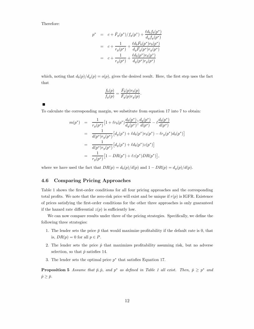
4.4 Optimal Pricing without Adverse Selection

We now consider a lender who optimizes his price without incorporating the effect of adverse

selection. That is, the lender is aware of risk but assumes that DR′(p) = 0 in setting his price.

The first order condition for profit maximization is:

Π ′(p) = d′(p)m(p) + d(p)[1−DR(p) −DR′(p)(p− c− `)] = 0 (13)

Setting DR′(p) = 0 and some algebra gives us the formula for the optimal price without adverse

selection, which we denote as p:

p = H(p) ≡ c+ `o(p) +1

r(p). (14)

We note that m(p) = (1 −DR(p))/r(p). Thus, if p exists, it will generate positive profit.

An alternative derivation of p can be obtained by assuming that the lender has initially set

a price p0 and has observed DR(p0) and r(p0). Then, not considering the dependence of DR

and r on p, he seeks to set a price p1 that satisfies the Equation 13 assuming DR′(p) = 0. In

this case, he would update his price to p1 according to:

1 −DR(p0)

(p1 − c)(1 −DR(p0)) − `DR(p0)= r(p0)

or, expressed as a general recursion:

pk+1 = c+ `o(pk) +1

r(pk). (15)

If the sequence defined by Equation 15 converges, it will converge to p: thus p would be the price

charged by a lender who continually observes default rates and adjusts his price to maximize

profitability given his current default rate.

4.5 Optimal Pricing with Adverse Selection

Finally, we consider the case of a lender who fully maximizes profit. The first-order conditions

for Equation 8 give:

1 − z(p∗)o(p∗)` = rg(p∗)(p∗ − c− `o(p∗)), (16)

where p∗ is the profit maximizing price. An implication of Corollary 1 is that, for k0 defined

in Equation 12, if z(p) > k0 for p ≥ c, then no p∗ satisfying Equation 16 can exist. Lemma 2

shows that the converse is also true.

Lemma 2 If there exists an ε > 0 such that ε ≤ z(p) < k0 as defined in Corollary 1 for all

p > c, then there exists a profit-maximizing price p∗ satisfying Equation 16.

Proof. The conditions for p∗ to exist are a direct consequence of proposition 3. Because

z(p) ≥ ε, we must have:

o(p) ≥ o0eεp

10

from Equation 6. Thus, there exists some p+ such that m(p) < 0 for p > p+. Thus, there must

exist a finite profit-maximizing price and it must satisfy 16.

Figure 4.5 shows the dependence of total profit on k in the case when the hazard rate z(p)

is equal to a constant k. This figure shows profit, Π(p) as a function of p for k = 0, .5, 1, 2. For

this example, ` = .9, c = 1, and o0 = .25. Lemma 2 shows that there is a profitable price for

k < k0 and no profitable price for k > k0 where k0 ≈ .7626 solves Equation 12. As shown in the

figure, there is a profitable region of prices for k = and k = .5 but not for k = 1 and k = 2.

Figure 2: Dependence of total profit Π(p) on p for various values of the hazard rate difference k when

z(p) = k is constant. For this example, ` = .9, c = 1, and o0 = .25. The normalized price responses for goods

and bads are both exponential c.c.d.f.’s so that di(p) = die−λp for i = g, b. For this example λg = 3 and

λb = λg − k for k = 0, .5, 1, 2.

Finally, we derive the first order condition for the profit-maximizing price when it does exist.

Proposition 4 If a profit-maximizing price exists in a segment displaying adverse selection, it

satisfies:

p∗ = c +1

rg(p∗)+ `o(p∗)

rb(p∗)

rg(p∗)(17)

Proof. We note first that profit can be written as:

Π(p) = (p − c)dgFg(p) − `dbFb(p) (18)

Taking the derivative and setting to 0, we must have:

0 = dgF (p∗) − (p∗ − c)dgfg(p∗) + `dbfb(p∗)

11

Therefore:

p∗ = c+ Fg(p∗)/fg(p

∗) +`dbfb(p

∗)

dgfg(p∗)

= c+1

rg(p∗)+`dbFb(p

∗)rb(p∗)

dgFg(p∗)rg(p∗)

= c+1

rg(p∗)+`db(p

∗)rb(p∗)

dg(p∗)rg(p∗)

which, noting that db(p)/dg(p) = o(p), gives the desired result. Here, the first step uses the fact

that

fb(p)

fg(p)=Fb(p)rb(p)

Fg(p)rg(p).

To calculate the corresponding margin, we substitute from equation 17 into 7 to obtain:

m(p∗) =1

rg(p∗)

[

1 + `rb(p∗)db(p

∗)

dg(p∗)

]dg(p∗)

d(p∗)− `

db(p∗)

d(p∗)

=1

d(p∗)rg(p∗)

[

dg(p∗) + `db(p

∗)rb(p∗) − `rg(p

∗)db(p∗)

]

=1

d(p∗)rg(p∗)

[

dg(p∗) + `db(p

∗)z(p∗)]

=1

rg(p∗)

[

1 −DR(p∗) + `z(p∗)DR(p∗)]

,

where we have used the fact that DR(p) = db(p)/d(p) and 1 −DR(p) = dg(p)/d(p).

4.6 Comparing Pricing Approaches

Table 1 shows the first-order conditions for all four pricing approaches and the corresponding

total profits. We note that the zero-risk price will exist and be unique if r(p) is IGFR. Existence

of prices satisfying the first-order conditions for the other three approaches is only guaranteed

if the hazard rate differential z(p) is sufficiently low.

We can now compare results under three of the pricing strategies. Specifically, we define the

following three strategies:

1. The lender sets the price p that would maximize profitability if the default rate is 0, that

is, DR(p) = 0 for all p ∈ P .

2. The lender sets the price p that maximizes profitability assuming risk, but no adverse

selection, so that p satisfies 14.

3. The lender sets the optimal price p∗ that satisfies Equation 17.

Proposition 5 Assume that p, p, and p∗ as defined in Table 1 all exist. Then, p ≥ p∗ and

p ≥ p.

12

Pricing

Approach Formula Profit (Π)

Zero-Risk p = c+ 1r(p)

dg(p)[1

r(p)− o(p)`]

Constant Margin pµ = c+ `o(pµ) +µd(pµ)

1−DR(pµ) µd(pµ)

Optimal wo. Adv. Sel p = c + `o(p) + 1r(p) dg(p)/r(p)

Optimal with Adv. Sel p∗ = c+ 1rg(p∗)

+ `o(p∗) rb(p∗)rg(p∗)

1rg(p∗)

[dg(p∗) + `z(p∗)db(p

∗)]

Table 1: Formulae and margins for four pricing approaches.

Proof. The conditions for the three prices are:

p = c+1

r(p)

p = c+ `o(p) +1

r(p)

p∗ = c+1

rg(p∗)+ `o(p∗)

rb(p∗)

rg(p∗)

The first price inequality is immediate because `o(p) > 0. The second price inequality requires,

1

rg(p)+ `o(p)

rb(p)

rg(p)≤ `o(p) +

1

r(p),

which follows from the fact that rb(p) ≤ r(p) ≤ rg(p) by hazard rate dominance.

It is instructive to compare optimal prices with and without adverse selection. Specifically,

consider the case of a segment characterized by some o0, z(p), and ` such that a profitable, profit-

maximizing price p∗ exists with corresponding default rate DR(p∗). Now, consider a segment

of equal size with the same value of ` and c but with z(p) = 0 for all p and with constant

default rate DR = DR(p∗). In other words, the second segment does not display adverse

selection but has a constant default rate equal to the optimal default rate of the first segment.

By proposition x, a profit-maximizing price p∗∗ must exist. Then, the following proposition

describes the relationship between the optimal prices and margins in the two segments.

5 Adverse Selection and Scoring

The discussion in the previous section focused on the problem of setting a single price to a seg-

ment of prospective lenders. We assumed that ex ante, the lender knows the number of “goods”

and “bads” in the underlying segment as well as how the “goods” and “bads” will respond to the

price that he offers. However, the lender has no available mechanism for distinguishing between

the “goods” and the “bads”. In this situation, the lender’s decisions are whether or not to offer

loans to the segment and, if so, what rate to charge.

13

In practice, lenders do not usually face a single homogeneous segment of prospective lenders

to which they will offer a single price. Rather, they seek to estimate the risk associated with

lending to a particular customer. Based on the lender’s estimate of the risk associated with

a customer, a lender may choose whether or not to approve an application (the underwriting

decision) and, if the lender approves the application, what price to charge. The underwriting

and pricing approach followed by many lenders can be summarized in four steps:

1. A prospective borrower applies for a loan.

2. The lender estimates the risk associated with making the loan to that customer.

3. Based on the estimated risk, the lender decides whether or not to offer the loan. If the

loan is offered, the lender must also decide on the price.

4. Assuming that the lender has decided to offer a loan, the borrower decides whether or not

to accept the loan at the offered price.

This is a highly stylized version of the process, which can vary for different markets and lenders.

For mortgages, a lender may offer a variety of different products – 15-year fixed, 30-year fixed,

5-year ARM, etc. – at different rates. The underwriting decision may not be a strict “yes” or

“no” but may take the form of restrictions or additional requirements on the borrower – for

example, mortgage insurance or a higher down-payment.

The most common approach in North America and Western Europe to quantify the risk

associated with a prospective borrower is some form of credit scoring. Let θi ∈ <N refer to

a vector of observable customer characteristics associated with customer i. Typically, these

characteristics are contained in the customer’s credit file and relate to various aspects of the

customer’s current financial commitments. For example, an Equifax credit file in Canada con-

tains 132 elements associated with a borrower such as number of accounts more than 30 days

past due, number of defaults in last 120 days, etc. A credit score is a scalar function s(θ) such

that ceteris paribus a higher value of the credit score is associated with a lower probability of

default. Typically, credit scores are positive integer values. For example, the FICO score used

in the United States spans a range from 300 to 800 with 300 the worst possible score and 800

a “perfect” score (Poon [2009]). Scores are commercially available through credit bureaus such

as TransUnion and Equifax. In addition, lenders often generate their own scores using a combi-

nation of commercially available credit data and internal customer data. There is a substantial

literature describing different approaches to computing and using credit scores; see, for example,

Thomas et. al. (2002) and de Servigny and Renault (2004).

We consider the case of a lender who is offering a single price to a segment such that

each customer within the segment has a credit score s with s ∈ [sL, sU ] ⊂ Z+. We assume

that credit score is the only criterion used by the lender in underwriting so that all customers

with s ∈ [sL, sU ] are approved. This guarantees that there is no selection, either adverse or

otherwise, occurring across any customer characteristic not incorporated in the score. Let d(s)

be the number of approvals with score s and let D =∑

s d(s) be the total number of approvals.

Define g(s) = d(s)/D as the density function of scores across approved applications. Define

db(s) and dg(s) as the number of “bads” and “goods” respectively with score s that have been

approved so that db(s) + dg(s) = d(s) for all s. Let DRA(s) be the expected default rate for

14

all loans with score s. Here and it what follow, the subscript A indicates that the quantity over

approved loans. Then, from the point of view of the lender, db(s) is a binomial random variable

with mean DRA(s)d(s). The expected default rate across the entire set of approvals is:

DRA =

sU∑

s=sL

DRA(s)g(s). (19)

We are interested in deriving the expected default rate for the booked loans, given DRA(s), g(s),

and p. We assume in what follows that the price-sensitivity of “goods” and “bads” is independent

of score – in other words fb(p) and fg(p) do not depend on score. An important implication of

this assumption is that the scores provide a consistent ordering of the underlying segment in

terms of default rate. That is, if the same price is offered to lenders with different scores, the

segment with the lower score will have a higher default rate, no matter what price is offered.

The consistent ordering property implies that o0(si) ≥ o0(sj) for all si, sj ,∈ [sL, sU ] whenever

i < j where oo(s) ≡ db(s)/dg(s).

The expected default rate from booked loans with score s given price p is:

DRB(s|p) =DRA(s)Fb(p)

DRA(s)Fb(p) + [1 −DRA(s)]Fg(p), (20)

where the subscript B indicates that the quantity is calculated for the portfolio of booked loans.

We can also derive the density function of scores for booked loans given a price of p as:

gB(s|p) =[DRA(s)Fb(p) + (1 −DRA(s))Fg(p)]g(p)

DRAFb(p) + (1 −DRA)Fg(p); s ∈ [sL, sU ] (21)

The expected default rate across all booked loans is:

DRB(p) =

sU∑

s=sL

DRB(s|p)gB(s|p). (22)

We define total adverse selection TAS(p) as the derivative of the expected default rate for booked

loans with respect to price, that is,

TAS(p) =dDRB(p)

dp

=

sU∑

s=sL

∂DRB(s|p)∂p

gB(s|p) +

sU∑

s=sL

DRB(s|p)∂gB(s|p)∂p

(23)

≡ IAS(p) +DAS(p). (24)

We term the first term on the right hand side of Equation 23 indirect adverse selection and

denote it by IAS(p). Indirect adverse selection is the change in the default rate as price changes

due to the change in default rate for borrowers with the same score. The second term on the

right hand side of Equation 23 measures direct adverse selection DAS(p) – the change in the

expected default rate as price changes due to the shift in credit scores of booked loans. We note

that direct adverse selection only occurs when the same price is offered to a range a credit scores.

If there is only a single credit score in the segment, then there is no direct adverse selection.

Note that total adverse selection is the sum of indirect adverse selection and direct selection.

15

Lemma 3 The expected default rate for a portfolio of bookings is:

DRB(p) =DRAFb(p)

DRAFb(p) + (1 −DRA)Fg(p)(25)

Proof. Substituting Equations 21 and 20 into Equation 22 and reducing gives:

DRB(p) =

sU∑

s=sL

DRA(s)Fb(p)g(s)

DRAFb(p) + (1 −DRA)Fg(s)

=[ Fb(p)

DRAFb(p) + (1 −DRA)Fg(p)

]

sU∑

s=sL

DRA(s)g(s),

substituting from 19 gives the desired result.

Proposition 6 The elements of adverse selection are:

TAS(p) = z(p)DRB(p)(1 −DRB(p)) (26)

IAS(p) = z(p)E[DRB(s|p)(1 −DRB(s|p))] (27)

DAS(p) = z(p)[E[DR2B(s|p)] −DR2

B(p)] = z(p)var[DRB(s|p)] (28)

where the expectation and the variance are taken over booked loans.

Proof in Appendix.

The resemblance of Equation 26 to Equation 4 is clear and has a similar interpretation –

namely, the magnitude of adverse selection in a segment with diverse credit scores is low when

the expected default rate is close to 0 or close to 1. If z(p) is constant, then the expected total

average selection for a segment will follow the same relationship to expected default rate as that

shown in Figure 1.

Note that Direct Adverse Selection can be calculated immediately after pricing from the

distribution of scores among customers who have accepted the loan. However, Indirect Adverse

Selection cannot be observed until a statistically significant number of loans default – which can

be six months or more after the loans fund. It is therefore useful to have a bound on the fraction

of total adverse selection that is due to indirect versus direct causes. Define δU = DR(sU ) and

δL = DR(sL) – that is δU is the lowest expected default rate and δL is the highest among scores

in the segment. Also, let ζ(δ) =√

δ(1 − δ) for δ ∈ [0, 1].

Proposition 7 For DR(sL) > 0, the ratio of Indirect Adverse Selection to Total Adverse Se-

lection satisfies:

IAS(p)/TAS(p) ≥ 1 − δL − δU + 2δUδL + 2ζ(δL)ζ(δU ) ≥ 1 − δL (29)

Furthermore, the first bound is tight.

Proof in Appendix.

Table 2 shows the lower bound on IAS(p)/TAS(p) for various values of δL and δU . An

implication of proposition 7 is that, in most cases, we would expect Indirect Adverse Selection

to be higher in magnitude than Direct Adverse selection in most lending situations. Most

commercial lenders do not lend to segments whose expected default rate is greater than 10% or

so – and many lenders will not lend to segments whose expected default rate is greater than 2%.

16

ln(δL)

ln(δU ) -9 -8 -7 -6 -5 -4 -3 -2 -1 0

−∞ .999877 .999665 .999088 .997521 .993262 .981684 .950213 .864655 .632121 0

-10 .999981 .999866 .999450 .998146 .994320 .983448 .953103 .869241 .638607 4.5 E-05

-9 1 .999948 .999636 .998503 .994958 .984545 .954934 .872175 .642801 .000123

-8 1 .999859 .999009 .995927 .986272 .957877 .876949 .649694 .000635

-7 1 .999616 .997301 .988901 .962522 .884650 .660990 .000912

-6 1 .998953 .992632 .969612 .896877 .679423 .002479

-5 1 .997133 .979733 .915271 .702940 .006738

-4 1 .992052 .943046 .756605 .018316

-3 1 .977162 .828739 .049787

-2 1 .926282 .135335

-1 1 .367879

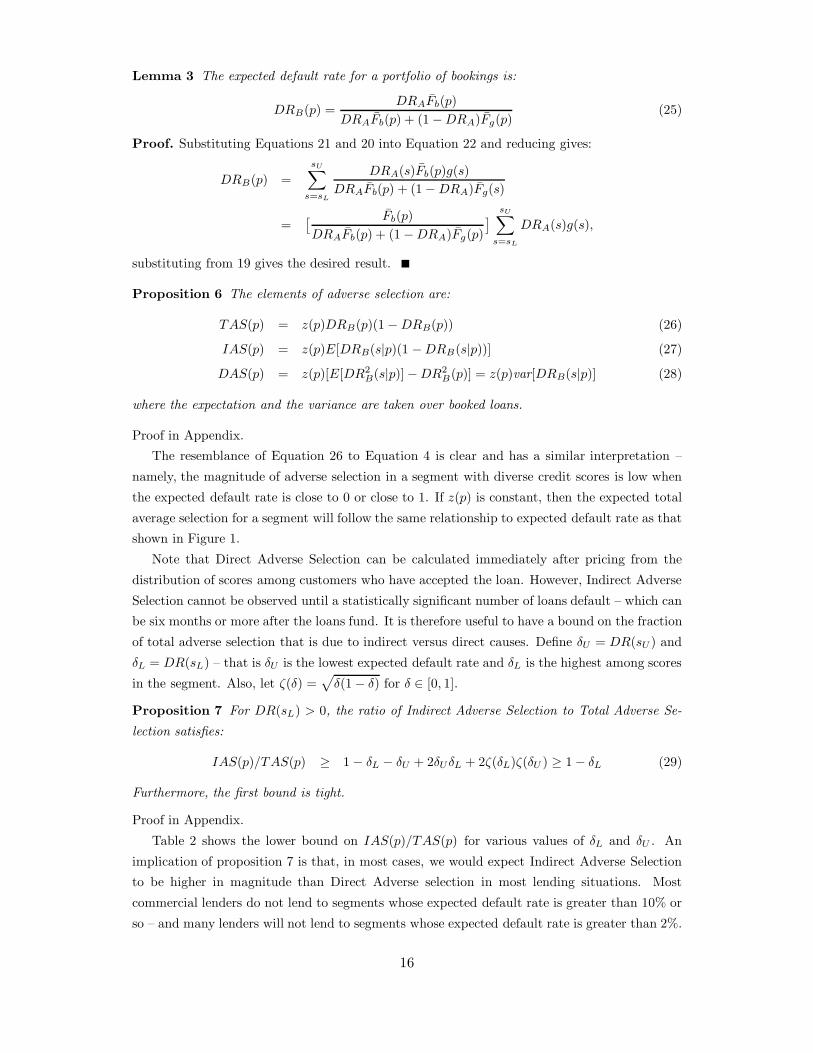
Table 2: Lower bound on IAS(p)/TAS(p) as a function of the highest and lowest expected default rates.

The first row represents the case in which δU = 0.

5.1 Underwriting and Pricing with Scoring

A lender with access to credit scores faces two decisions: which prospective lenders to accept

and what price(s) to charge to those that are accepted. We assume as before that the scores

incorporate all of the information about prospective borrowers relevant to risk. In order to

characterize the underwriting and pricing decisions, we need to recognize that the marginal cost

of loans may depend upon the score of the borrower. Basel II and related regulations require

that banks maintain capital reserves who size in part depends on the riskiness of their portfolios.

Because of this, a lender may need to set aside more reserves when lending to a risky customer

(one with a lower score) than a less risky customer. The cost of the additional reserves is

typically calculated as the lost risk-free return on the reserve for the term of the loan. While

the detailed calculation of the capital cost that should be assigned to a particular loan can be

complex, the cost will be an increasing function of risk and thus a decreasing function of score,

that is c(si) ≥ c(sj) for i < j; si, sj ∈ [sL, sU ].

We consider first a lender who has full autonomy to determine which scores to accept and

which to reject and has total freedom to charge customers with different scores differently.

Proposition 8 A profit-maximizing lender with full pricing flexibility and a segment with scores

s ∈ [sL, sU ] would adopt one of two policies:

1. Not lend to any prospective borrower.

2. Set a minimum s ∈ [sL, sU ] and lend to all borrowers with s ∈ [s, sU ], charging a price to

each approved borrower of p∗(s) = c(si) + 1rg(p∗(s)) + `o(p∗|s) rb(p∗(s))

rg(p∗(s)) ,

where o(p∗|s) are the odds at price p∗ given score s.

Proof. Clearly, a profit-maximizing lender with full pricing flexibility would choose to lend to

every score for which there is a profitable price and would do so at the profit-maximizing price

17

as defined in Equation 17. It remains to be shown that, if it is unprofitable to lend to score si,

then it is unprofitable to lend to score si−1. By the consistency of the scores o0(si−1) ≥ o0(si).

Assume that it is unprofitable to lend to score si. Then:

m(p|si) = (p − c(si))(1 −DR(p|si)) − `DR(p|si) ≤ 0 for p > c(si),

where m(p|s) is the margin for a loan at price p to customers of score s. But, o0(si−1) ≥o0(si) −→ DR(p|si−1) ≥ DR(p|si) for all p > c(si−1). Thus, m(p|si−1) ≤ m(p|si) ≤ 0 for all

p > c(si−1) > c(si) and it is unprofitable to lend to borrowers with score si−1.

We note that the prices p∗(s) will be decreasing in score.

On the other end of the spectrum, a lender might offer only a single price, independent of

credit score. We can show that a cutoff policy is also optimal for such a lender.

Proposition 9 A profit-maximizing lender who can only charge a single price would adopt one

of two policies:

1. Not lend to any prospective borrower.

2. Set a minimum s ∈ [sL, sU ] and lend to all borrowers with s ∈ [s, sU ].

Proof. We observe that the profit margin m(p|s) is increasing in s for all p because both

DR(p|s) and c(s) are decreasing in s. Thus, for any p, if it is optimal to lend to customers with

score si−1, it is also profitable to lend to customers with score si.

We note the following relationship between the optimal cutoff score for the fully flexible pricing

policy s and the cutoff score for the single-price policy s.

Corollary 2 Given any distribution of scores on [sL, sU ], s ≤ s.

Proof. Let p∗ be the optimal single price. Then, it must be that (p∗ − c)(1 − DR(p|s)) −`DR(p|s) ≥ 0, otherwise the lender could increase profitability by setting s = s + 1 or by not

lending at all if s = sU . Therefore, a fully-flexible lender would choose to lend to customers

with score s.

In reality, most lenders do not follow either of the two pure policies. A common practice is to

divide scores into a smaller number of mutually exclusive risk bands: [s0, s1), [s1, sn), . . . , [sn, sU ].

Applicants with scores in [s0, s1) will be rejected while applicants in the other risk bands will

be accepted and charged a rate pi where i is the index of the risk band [si, si+1). Reasons

often given for charging fewer rates than credit scores include limitations in the software used

to set and/or communicate prices as well as a desire to keep pricing policies simple so they can

be easily understood and communicated. In any case, the results of propositions 8 and 9 and

Corollary 2 hold for risk bands as for individual risk scores.

6 Conclusions and Future Research

This paper showed that a relatively simple model of differential price-sensitivity can be used to

derive a model of price-driven adverse selection that explains a number of real-world phenomena.

In our model, adverse selection is strongly driven by the difference in the price-response hazard

18

rates displayed by goods and bads. In particular, a higher hazard-rate differential leads to a

higher rate of price-driven adverse selection. We show that, ceteris paribus, a sufficiently high

hazard rate differential will lead to a situation in which it is unprofitable to lend to a market

segment at any price.

One area for further investigation is the role of affordability or capacity effects in default. Our

model has assumed that the decision of an individual borrower to default is independent of the

rate, that is, borrowers can ex ante be sorted into “goods” and bads. However, it is possible that

a higher monthly payment could increase stress in a borrower that would lead to an increased

likelihood of default. In this case, there would not be fixed values of dg and db – instead, the

number of “bads” would increase with the price. Our model could be modified to incorporate

such an effect by including an increasing function h(p) such that Db(p) = db + h(p)dg where db

and dg can now be interpreted as the number of “bads” and “goods” in the population assuming

a price of 0, D(p) is the total number of bads in the population at price p and 0 ≤ h(p) ≤ 1

specifies the rate at which goods become bads as a function of price.

7 Acknowledgment

This research was funded in part by the US Federal Deposit Insurance Corporation Center for

Financial Research.

8 Appendix

Proof of proposition 3

First we note that Equation 11 has a unique root kµ with 0 < kµ < e−1/`(o0 + µ) because

the right hand side of Equation 11 decreases from e−1/[o0(`+µ)] to 0 as kµ increases to infinity.

Substituting from Equation 5 into Equation 10 means that pµ must solve:

p = c+ `A(p)o0 + µ[1 −DR(0) +DR(0)A(p)

1 −DR(0)

]

= c+ `A(p)o0 + µ(1 + o0A(p))

which implies p− c− µ = o0A(p)(`+ µ), where A(p) is defined in Equation 5. Let z(p) = k and

take logarithms of both sides to obtain;

ln(p− c− µ) = ln(`+ µ) + ln(o0) + kp. (30)

The left side of Equation (30) is concave in p and strictly increases from −∞ at p = c+µ to ∞.

The derivative of ln(p−c−µ) w.r.t. p decreases from ∞ at p = c+µ continuously toward 0. Taken

together, these mean that, for any value of k > 0 there is a unique p(k) > c such that there exists

a line with slope k that is tangent to ln(p− c− µ) at p(k). Denote the intercept of this line by

(0, a(k)). Since the slope at p(k) is k, we must have k = [∂ln(p− c− µ)/∂p]|p(k) = 1/(p(k)−c−µ)

which implies that p(k) = c+µ+1/k and ln(p(k)−c−µ) = − ln(k). It can be easily be calculated

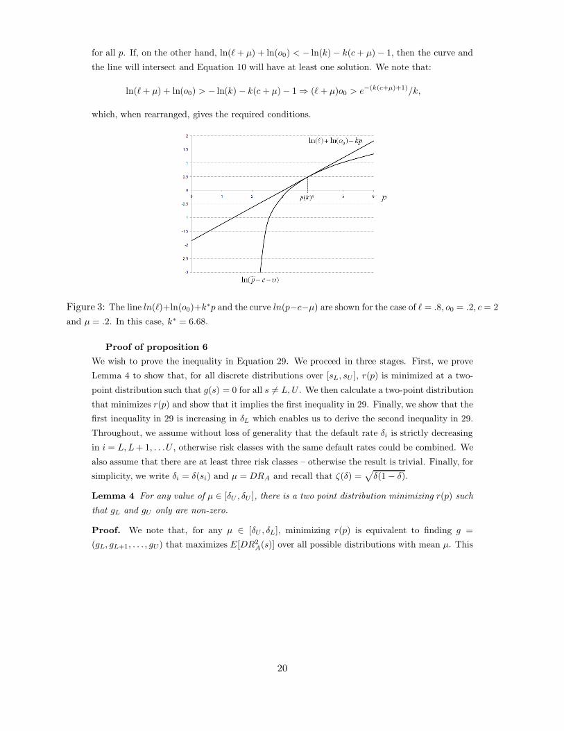
that a(k) = − ln(k)−k(c+µ)−1. As shown in Figure 3, if ln(`+µ)+ln(o0) > − ln(k)−k(c+µ)−1,

then the line ln(`+µ)+ln(o0)+kp will always be above the curve ln(p−c−µ) so that m(p) < µ

19

for all p. If, on the other hand, ln(` + µ) + ln(o0) < − ln(k) − k(c+ µ) − 1, then the curve and

the line will intersect and Equation 10 will have at least one solution. We note that:

ln(`+ µ) + ln(o0) > − ln(k) − k(c + µ) − 1 ⇒ (` + µ)o0 > e−(k(c+µ)+1)/k,

which, when rearranged, gives the required conditions.

Figure 3: The line ln(`)+ln(o0)+k∗p and the curve ln(p−c−µ) are shown for the case of ` = .8, o0 = .2, c = 2

and µ = .2. In this case, k∗ = 6.68.

Proof of proposition 6

We wish to prove the inequality in Equation 29. We proceed in three stages. First, we prove

Lemma 4 to show that, for all discrete distributions over [sL, sU ], r(p) is minimized at a two-

point distribution such that g(s) = 0 for all s 6= L, U . We then calculate a two-point distribution

that minimizes r(p) and show that it implies the first inequality in 29. Finally, we show that the

first inequality in 29 is increasing in δL which enables us to derive the second inequality in 29.

Throughout, we assume without loss of generality that the default rate δi is strictly decreasing

in i = L, L+ 1, . . .U , otherwise risk classes with the same default rates could be combined. We

also assume that there are at least three risk classes – otherwise the result is trivial. Finally, for

simplicity, we write δi = δ(si) and µ = DRA and recall that ζ(δ) =√

δ(1 − δ).

Lemma 4 For any value of µ ∈ [δU , δU ], there is a two point distribution minimizing r(p) such

that gL and gU only are non-zero.

Proof. We note that, for any µ ∈ [δU , δL], minimizing r(p) is equivalent to finding g =

(gL, gL+1, . . . , gU) that maximizes E[DR2A(s)] over all possible distributions with mean µ. This

20

can be written as a linear program:

maxgV (g) ≡

U∑

i=L

giδ2i (31)

s.t.

U∑

i=L

giδi = µ

U∑

i=L

gi = 1

g ≥ 0

From complementary slackness, it must be that there is a g∗ that solves the linear program 31

such that at most two elements of g∗ are greater than 0 with all other elements equal to zero.

Let g∗i , g∗

j ∈ [gL, gU ] be those two values with g∗i < g∗j and let δ∗i and δ∗j the corresponding

default rates. Note that δ∗j < µ < δ∗i , so, we must have g∗i δ∗

i + (1 − g∗i )δ∗j = µ, which implies

that:

g∗i = (µ− δ∗j )/(δ∗i − δ∗j ) and g∗j = (δ∗i − µ)/(δ∗i − δ∗j ).

Substituting into the objective function in Equation 31 gives:

V (g∗) =(µ− δ∗j )(δ∗i )2 + (δ∗L − µ)(δ∗j )2

δ∗i − δ∗j

= µ(δ∗i + δ∗j ) − δ∗i δ∗

j .

Because δ∗j < µ < δ∗i , V (g∗) is increasing in δ∗i and decreasing in δ∗j . Thus, we must have that

δ∗j = δU and δ∗i = δL.

For any value of µ, r(p) is minimized by a two point distribution such that gL = (µ −δU )/(δL − δU ) and gU = (δL −µ)/(δL − δU ) and gi = 0 for all i 6= L, U . The corresponding value

of E[DR2A(s)] = µ(δL + δU ) − δLδU . This means that the lower bound on r(p) can be found by

solving the optimization problem:

minµψ(µ) ≡ µ(1 − δL − δU ) + δLδU

µ(1 − µ)(32)

subject to δU ≤ µ ≤ δL. Taking the derivative of ψ(µ) and setting equal to zero gives the first

order condition:

0 = (1 − δL − δU )(µ∗)2 + 2δLδUµ∗ − δLδU

The only positive root of this equation is:

µ∗ =ζ(δL)ζ(δU ) − δLδU

1 − δL − δU(33)

The first bound in 29 can be obtained by substituting the expression for µ∗ in Equation 33 into

the objective function in Equation 32 and performing some algebra.

21

To obtain gL and gU , we substitute Equation 33 back into the formula for gL to obtain:

gL =ζ(δL)ζ(δU ) − δLδU − δU (1 − δL − δU )

(δL − δU )(1 − δL − δU )

=ζ(δL)ζ(δU ) − ζ2(δU )

ζ2(δL) − ζ2(δU )

=ζ(δU )

ζ(δU ) + ζ(δL),

which means that gU = ζ(δL)/[ζ(δU ) + ζ(δL)].

We now need to show the second inequality in 29. Define ρ(δU , δL) = r(p), that is ρ is the

lower bound parameterized with δU and δL. We show that ∂ρ(δU , δL)/∂δU ≥ 0. Note that

ρ(δU , δL) can be written as ρ(δU , δL) = [√δLδU +

√

(1 − δL)(1 − δU )]2. Since both terms that

are being squared are greater than or equal to zero, we only need to consider the derivative of

the terms inside the bracket. That is, we can calculate:

∂[√δUδL]

∂δU+∂[

√

(1 − δU )(1 − δL)]

∂δU=

√δL

2√δU

−√

1 − δL

2√

1 − δU.

This partial derivative will be greater than or equal to zero if√

δL(1 − δU ) ≥√

δU (1 − δL). But

this inequality is guaranteed to hold since δL ≥ δU .

References

[1] Agarwal, S., Chomsisengphet, S., and Liu, C. n.d. “Adverse Selec-

tion in the Credit Card Market: Evidence from a Natural Experi-

ment” Working Paper, The Federal Reserve Bank of Chicago, available at

http://www.geocities.com/ushakri/CreditCardAdvSelection.pdf+agarwal+%22natural+experiment%22.

[2] Akerlof, G. A. 1970. “The Market for ’Lemons’: Quality Uncertainty and the Mar-

ket Mechanism”. Quarterly Journal of Economics 84 3: 488500.

[3] Altman, D., Cutler, D. M., and Zeckhauser, R. J. 1998. “Adverse Selection and

Adverse Retention.” AEA Papers and Proceedings 88 2.

[4] Ausubel, L. 1999. “Adverse Selection in the Credit Card Market.” Working Paper.

University of Maryland.

[5] Balakrishnan, N. (ed.) 1992. Handbook of the Logistic Distribution, Marcel Dekker,

Inc. New York.

[6] Barlow, R. E. and Proschan, F. 1965. Mathematical Theory of Reliability. John

Wiley and Sons, New York.

[7] Bergstresser, D. and J. Bashears. 2009. “Who Selected Adjustable-Rate Mortgages?

Evidence from the 1989-2007 Surveys of Consumer Finance,” Working Paper. Na-

tional Bureau of Economic Research.

22

[8] Burks, S. V., Carpenter, J. V., Goette, L., and Rustichini, A. 2009. “Cognitive Skills

Affect Economic Preferences, Strategic Behavior, and Job Attachment,” Proceed-

ings of the National Academy of Sciences. 106 19: 7745-7750.

[9] de Servigny, A. and Renault, O. 2004. Measuring and Managing Credit Risk Mc-

Graw Hill: New York, NY.

[10] Engelmann, B. and Rauhmeier, R. (eds.) 2006 The Basel II Risk Parameters:

Estimation, Validation, and Stress Testing. Springer Verlag: Heidelberg, Germany.

[11] Genesove, D. 1993. “Adverse Selection in the Wholesale Used Car Market,” Journal

of Political Economy 101: 644-645.

[12] Edelberg, W. 2004. “Testing for Adverse Selection and Moral Hazard in Consumer

Loan Markets”, Finance and Economics Discussion Series 2004-9, The US Federal

Reserve: Washington, DC.

[13] Edelberg, W. 2006. “Risk-based Pricing of Interest Rates for Consumer Loans,”

Journal of Monetary Economics 53 8: 2283-2298.

[14] Gerardi, K., Goette, L., and Meier, S. 2009. “Sustainable Homeownership and

Numerical Ability,” Working Paper. Federal Reserve Bank of Atlanta.

[15] Karlan, D. S. and Zinman, J. 2005. “Observing Unobservables: Identifying

Information Asymmetries with a Consumer Credit Field Experiment,” Yale

University Economic Growth Center Discussion Paper No. 911. Available at

http://ssrn.com/abstract=725563.

[16] Lariviere, M. A. 2006. “A Note on Probability Distributions with Increasing Gen-

eralized Failure Rates” Operations Research 54 3: 602-604.

[17] Lariviere, M. A. and Porteus, E. 2001. “Selling to a Newsvendor: An Analysis

of Price-Only Contracts”. Manufacturing Service OPerations Management. 3 4:

293-305.

[18] Phillips, R.L. 2005. Pricing and Revenue Optimization. Stanford University Press:

Stanford, CA.

[19] Phillips, R. L. 2009. “An Introduction to Price Optimization for Consumer Credit,”

forthcoming in Credit Control.

[20] Poon, M. 2007. “Scorecards as Devices for Consumer Credit: The case of Fair,

Isaac & Company Incorporated” in Market Devices. Eds. M. Callon, F. Muniesa

and Y. Millo. Blackwell Publishing, London.

[21] Shaked and Shantikumar. 2007. Stochastic Orders Springer: New York, NY.

[22] A. Smith. 1776 The Wealth of Nations. Reprinted 2000. Modern Library: New

York, NY.

23

[23] Stiglitz, J. E. and Weiss, A., 1981. “Credit Rationing in Markets with Imperfect

Information,” American Economic Review, 71 3: 393 - 410.

[24] Thomas, L. C., 2009. Consumer Credit Models: Pricing, Profit, and Portfolios

Oxford University Press, Oxford, UK.

[25] Thomas, L.C., Edelman, D. B., and Crook, J. N. 2002. Credit Scoring and Its

Applications SIAM. Philadelphia, PA.

[26] van den Berg, G. J., 2007. “On the Uniqueness of Optimal Prices Set by Monopo-

listic Sellers,” Journal of Econometrics. 141 482-491.

[27] Wilkinson, G. and Tingay, J. 2004. “The use of Affordability Data – Does it add

Real Value,” in Readings in Credit Scoring, eds. Thomas, L. C.; Edelman, D. B.;

Crook, J. N. Oxford University Press. Oxford, UK.

[28] Wimmer, B. S. and Chezum, B., 2006. “Adverse Selection, Seller Effort, and Se-

lection Bias,” Southern Economic Journal, 73 1: 201-218.

[29] Ziya, S., Ayhan, H.. and Foley, R. D., 2004. “Relationships Among Three Assump-

tions in Revenue Management,” Operations Research. 52 5: 804-809.

24