Price Formation and Exchange in Thin Markets:

A Laboratory Comparison of Institutions*

by

Timothy N. CasonUniversity of Southern California

and

Daniel FriedmanUniversity of California, Santa Cruz

Draft: June 1996

Abstract

This paper compares the performance of four different trading institutions in laboratory markets.Two institutions, the continuous double auction and the single call market, are commonlyemployed on organized exchanges. Two other “hybrid” institutions, the uniform price doubleauction and multiple call market, link the other institutions in different dimensions. The laboratoryenvironment features four buyers and four sellers who receive random values and costs in eachperiod and who have a one-unit trading capacity. Therefore, each period provides an observationof price formation and exchange in a thin market environment. We find that trading efficiency islowest in the institutions that permit only one transaction opportunity each period, primarily due toinsufficient trading volume. However, the institutions that permit a single trading opportunityforce all traders to transact at a uniform price, which tends to generate prices that more accuratelyreflect underlying market conditions.

*This is a revision of a draft presented at “Money, Markets and Methods: A Conference in Honorof Robert Clower,” Department of Economics, University of Trento (9-10 May 1996). Financialsupport was provided by the National Science Foundation (SES-9223830). We gratefullyacknowledge the programming support of Andrew Davis and Tai Farmer and the researchassistance provided by Carl Plat and Feisal Khan. We received helpful comments from Jim Cox,Robert Clower, Peter Howitt, Angel Palerm, and other participants at the Trento converence andthe Spring 1995 Economic Science Association/Public Choice Society meetings.

1

Progress in economic theory...depend[s] crucially on development of an

empirically acceptable theoretical account of the market institutions that sustain

coordinated exchange activity in the world of our everyday lives.

--Clower and Howitt (1996, page 34)

1 . Preface

In this paper we accept the Clower and Howitt challenge, and take some empirical steps

towards understanding market institutions. Our institutions and procedures will not be familiar to

all readers, so we begin by offering four assertions and a caveat.

1. Market institutions matter. Clower and various co-authors have convincingly argued that

macroeconomics and monetary economics can not properly address their central issues without a

serious account of market institutions (e.g., Clower and Howitt,1996, Clower 1977, 1975; see

also Okun 1981 inter alia). Market institutions exist in the world in order to solve the incentive,

coordination and logistical problems associated with price formation and exchange. The

institutions typically involve the exchange of money for a single homogeneous good (or subset of

related goods) and are organized by specialized middlemen (e.g., wholesalers or retailers or

brokers). The practical issues of macroeconomics -- the impact of shocks and policy interventions

on prices and quantities exchanged -- thus hinge on the performance characteristics of market

institutions.

Market institutions, we might add, are equally important to applied microeconomists and

financial economists. The standard economic tools presume equilibrium prices, so in choosing

where to use these tools economists rely on an implicit theory of price formation. Moreover many

policy interventions (ranging from job retraining programs to SEC reporting requirements in

securities markets) are intended to influence the adjustment to equilibrium, and therefore their

effectiveness depends entirely on how market institutions work.

2. The performance characteristics of market institutions are not well understood. The “institution-

free” textbook model of Arrow-Debreu (and its various simplifications and elaborations) simply

2

assumes that equilibrium is achieved immediately, and so ignores the coordination, logistical and

incentive problems of who transacts with whom and how they agree on price. Walras (1874) first

proposed to fill the logical gap with an artificial market institution called tâtonnement that precluded

transactions outside of equilibrium. Its performance characteristics were analyzed by many authors

including Hicks (1939), Samuelson (1948), and Arrow and Hurwicz (1958). The so- called non-

tâtonnement literature then arose in response to the objection that transactions might occur outside

of equilibrium; see Arrow and Hahn (1972) for an early survey.

This line of work presumes price-taking behavior or thick markets in which traders always

can buy or sell any desired quantity at the “going” price. What if traders set their own prices, not

necessarily uniformly? Smale (1976), together with extensions by Schechter (1975), Wan (1980),

and Friedman (1979), showed that virtually any individually rational Pareto Optimum (supported

by appropriate prices) could arise from such generalized non-tâtonnement processes; but this

literature offers little insight into the performance of any specific market institution. Most recent

models are search-theoretic, for example Gale (1987), Wollinsky (1990), and Kiyotaki and Wright

(1989). Unfortunately, as Clower and Howitt emphasize, such models rule out organized markets

as we know them; traders encounter each other at random or in exogenous (and inefficient) order.

An entrepreneur who opened an organized market using a reasonable institution would quickly take

over, and thus would alter the performance characteristics.

There are some relatively slender strands of theoretical literature that deal with actual market

institutions, mainly the continuous double auction (CDA) and the single call market (SCM). We

will present these strands in the next section; for now suffice it to say for now that we do not yet

have a logically complete and empirically verified characterization of market institutions’

performance.

3. Most markets are thin. They have few enough active traders that individual decisions can affect

price, but (unlike search models) they are organized. Depending on the actual market institution,

their performance may or may not be described well by the equations in Clower (1990). Market

thickness is endogenous, an evolutionary outcome driven by two opposing forces: network and

3

informational externalities that promote thickness, and diversity of taste (or of time and

circumstance) that promotes customization and fragmentation.1 The net result in most markets

(ranging from carpenters’ bids on small home improvement jobs to the interbank US Dollar-

Japanese Yen exchange market) seems to be between two and two dozen active traders at any given

time.

4. Laboratory methods are well suited for studying market institutions. They overcome two major

problems with field data. First, key variables such as equilibrium price and allocational efficiency

are not directly observable in the field. In the laboratory we can control buyers’ values and sellers’

costs and therefore measure market performance directly. Second, the market institution and

market thickness are selected endogenously in the field so inferences about their impact are

problematic. Suppose, for example, we find that a field market using the SCM institution is more

volatile than one using the CDA (Stoll and Whaley, 1990). We shouldn’t infer that the SCM

increases volatility because the volatility difference might be due to environmental differences.

Indeed, the SCM institution might have evolved precisely because it reduces volatility that

otherwise would be even higher. In laboratory markets we control the market institution and

market thickness and so can make valid inferences about their impact.

It should be noted that Robert Clower was among the first to recognize the value of

laboratory methods. In 1958 he ran several market experiments by hand at Northwestern

University, mainly Cournot oligopolies and monopolies with randomly shifting demand. The

findings influenced Clower (1959). Eventually he found it “found it too arduous to continue,”

[personal communication, 1996] a sentiment with which we certainly can sympathize, even with

the benefit of current labor-saving laboratory computer technology. Since then Clower has quietly

encouraged laboratory research by others and its publication in mainstream economics journals.

Caveat. Laboratory methods are not a panacea. One must sooner or later check for external

validity, which typically involves comparison to econometric analysis of field data. Thicker

markets are more expensive to run in the laboratory. The laboratory has fewer advantages for

studying the evolution of markets than it has for studying their performance characteristics. In

4

sum, laboratory markets are best used in conjunction with other tools including numerical

simulation, econometric analysis of field data, and formal analytics.

2 . Four Market Institutions

This paper reports a laboratory experiment with sessions conducted in four different trading

institutions. The institutions facilitate trade in homogeneous goods for which ongoing

relationships between buyer and seller are unimportant.2 The design holds the environment

(including public information, the number of traders and the realized values and costs) constant

while varying the trading institution in a nearly continuous fashion between those known to

promote competitive equilibrium outcomes and those known not to do as well. Figure 1 illustrates

the relationship between the institutions and summarizes the experimental design.

The two polar institutions employed in the study are the Continuous Double Auction (CDA)

and the Single Call Market (SCM). In the CDA, traders can make and accept offers to buy and to

sell at any moment in a trading period, so it is the richest in terms of within-period information

feedback, trading opportunities and strategic complexity. The CDA has also demonstrated

remarkably rapid convergence to CE in a wide variety of trading environments. The SCM is on the

opposite extreme. In the SCM, traders independently submit bids and asks that are aggregated into

demand and supply curves and cleared once at a uniform price each period. Information feedback

is non-existent during a trading period–which contains only one trading opportunity–and its

strategy space is highly restricted relative to the CDA. The SCM has also been shown to have

inferior performance characteristics relative to the CDA in stationary value environments (Smith et

al., 1982).

As illustrated above in Figure 1, the remaining two trading institutions link these polar

institutions along two different dimensions: (1) The number of trading opportunities and (2) the

amount of within-period information feedback. This provides insight into the particular institution

attributes affecting trader behavior and market performance. In multiple-call markets (MCM), like

the SCM traders independently submit bids and asks that are aggregated and the market is cleared

5

at a uniform price. In contrast to the SCM, however, in the MCM the market is cleared several

times per period. This institution helps determine the impact of an increased number of trading

opportunities per period, without the richness of the CDA information space. Of course, the MCM

institution also necessarily increases the amount of market feedback within the period along with

the number of calls, because traders observe whether or not they trade after each call. We

conducted 3, 5 and 8 calls per period in these sessions, with the 8-call markets most perceptually

similar to the CDA.3

The Uniform Price Double Auction (UPDA) markets determine the role of continuous

information feedback in the CDA institution’s performance, while limiting the number of trading

opportunities to one per period as in the SCM. In the UPDA, one call is held at the end of the

trading period, but during the period traders submit and revise market bids and offers while

observing changes in the possible terms of trade. Our UPDA experiments focus on an

environment with information conditions most similar to the CDA.

Our emphasis on the market institution is close in spirit to the literature surveyed in O’Hara

(1995) that examines the “microstructure” of asset markets. This research has used both theoretical

and empirical methods to investigate the “price discovery” (i.e., price formation) process under

various assumptions regarding the market institution. For example, Ho and Stoll (1983) focused

on the CDA institution and constructed a fairly complex dynamic programming model to predict

sequences of transaction prices and the bid-ask spread. Stoll and Whaley (1990) use field data

(from the NYSE) to compare the call market institution (at the opening of trade) to continuous

trading. Recent research in this area has compared the performance of the specialist market

institution to the competitive dealer institution (e.g., Affleck-Graves et al., 1994).

A leading theoretical approach to price formation regards traders as playing a game of

incomplete information defined by the market institution and the environment, and uses the concept

of Bayesian Nash equilibrium (BNE) to characterize behavior. Satterthwaite and Williams (1993)

and Rustichini, Satterthwaite and Williams (1994) take this approach to the SCM. They show that

traders generally have the incentive to misrepresent their true valuations: buyers typically want to

6

bid below redemption value and sellers typically want to ask above cost. They characterize the

degree of misrepresentation in BNE and show that it (and therefore the unrealized gains from trade

and the deviation of price from competitive equilibrium) falls fairly rapidly as the number of buyers

and sellers increases. Wilson (1987) applies the same approach to the CDA. Again assuming a

random values environment, he derives necessary conditions for BNE and obtains some efficiency

results. Cason and Friedman (1996) contains a more detailed discussion of his model.

This BNE approach assumes that traders are all unboundedly rational and have incredibly

good information (e.g., regarding each others’ contingent strategies). Researchers have also

adopted an alternative learning/Nash equilibrium (NE) approach to relax this rationality constraint

and improve the empirical validity of the theory. This approach allows traders to be initially

ignorant about the environment and the market institution, but assumes that experience causes

traders to adjust and improve their strategies incrementally. Friedman (1991b) and others show

under quite general conditions that if players (traders) achieve a behavioral steady state, then their

strategies at that point constitute (as-if complete information) Nash equilibrium. This approach

also underlies Friedman and Ostroy’s (1995) theoretical analysis of the SCM and the Friedman

(1991a) model of price formation in the CDA. The approach clearly influences other treatments of

the SCM including Satterthwaite and Williams (1993) and the CDA, e.g., Easley and Ledyard

(1993).

Several laboratory experiments are especially relevant to the present study. Smith et al.

(1982) compares performance of the CDA to several variants of the SCM. Price formation was

more rapid and reliable in the CDA but a multiple- unit, recontracting version of the SCM had

equivalent allocational efficiency. Friedman and Ostroy (1995) find that both the CDA and the

SCM eventually produce highly efficient allocations even when the induced values and costs are

chosen to encourage strategic misrepresentation. McCabe et al. (1993) study UPDA in an

environment with additive random shifts superimposed each period on otherwise repetitively

stationary demand and supply schedules. Friedman (1993) examines another variant of the UPDA

institution as well as the MCM institution in an asset market environment. These studies find that

7

the best variants of UPDA and MCM are almost as reliable as the CDA in producing prices and

allocations near competitive equilibrium.

None of the last four articles systematically examines the price formation process. Price

formation in the CDA is the focus of Cason and Friedman (1993 and 1996). There we compare

the abilities of a BNE model, a learning/NE model and a zero intelligence model (Gode and

Sunder, 1993) to explain the process in simple random environments. Each model has some

limited success in explaining different aspects of the price formation process. Kagel and Vogt

(1993) and Cason and Friedman (1997) test the Satterthwaite-Williams model of price formation

for the SCM, and Kagel (1994) studies both the SCM and CDA in identical environments. These

studies were conducted using a random values environment, and typically find departures from

BNE behavior. These departures are attributed primarily to inadequate or biased learning.

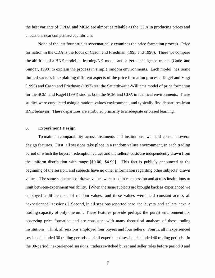
3 . Experiment Design

To maintain comparability across treatments and institutions, we held constant several

design features. First, all sessions take place in a random values environment, in each trading

period of which the buyers’ redemption values and the sellers’ costs are independently drawn from

the uniform distribution with range [$0.00, $4.99]. This fact is publicly announced at the

beginning of the session, and subjects have no other information regarding other subjects’ drawn

values. The same sequences of drawn values were used in each session and across institutions to

limit between-experiment variability. [When the same subjects are brought back as experienced we

employed a different set of random values, and these values were held constant across all

“experienced” sessions.] Second, in all sessions reported here the buyers and sellers have a

trading capacity of only one unit. These features provide perhaps the purest environment for

observing price formation and are consistent with many theoretical analyses of these trading

institutions. Third, all sessions employed four buyers and four sellers. Fourth, all inexperienced

sessions included 30 trading periods, and all experienced sessions included 40 trading periods. In

the 30-period inexperienced sessions, traders switched buyer and seller roles before period 9 and

8

before period 25; in the 40-period experienced sessions, traders switched roles before period 11

and before period 31. This switch was common knowledge, as was the number of buyers and

sellers in each session. The remainder of this section provides additional design details for each

institution.

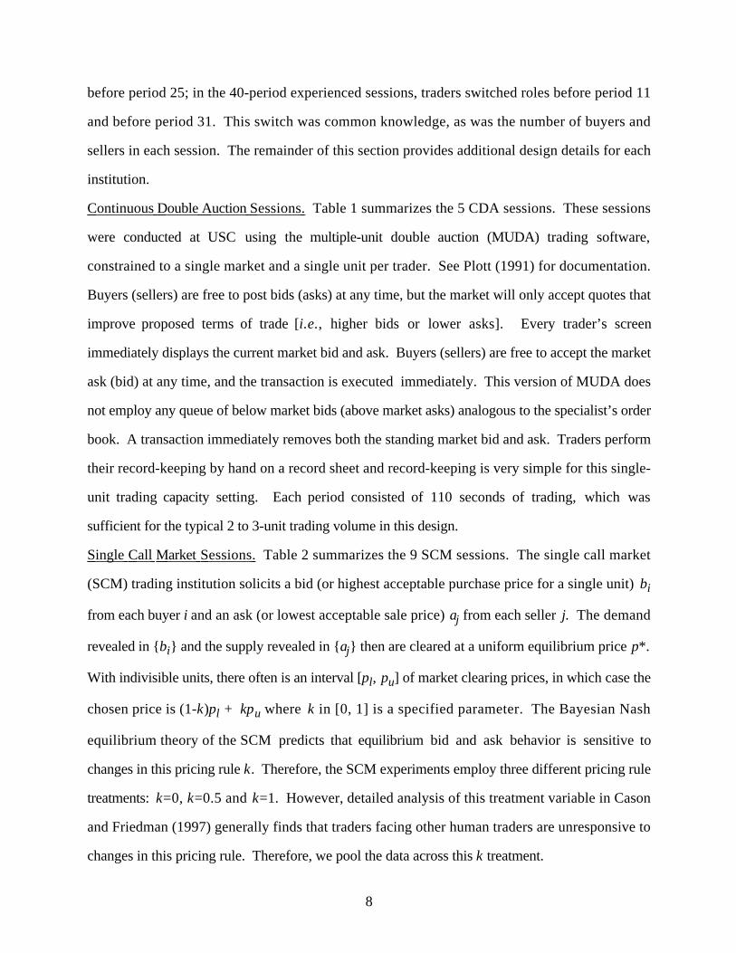
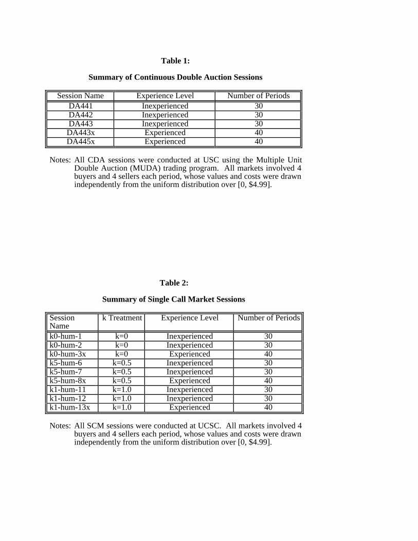
Continuous Double Auction Sessions. Table 1 summarizes the 5 CDA sessions. These sessions

were conducted at USC using the multiple-unit double auction (MUDA) trading software,

constrained to a single market and a single unit per trader. See Plott (1991) for documentation.

Buyers (sellers) are free to post bids (asks) at any time, but the market will only accept quotes that

improve proposed terms of trade [i.e., higher bids or lower asks]. Every trader’s screen

immediately displays the current market bid and ask. Buyers (sellers) are free to accept the market

ask (bid) at any time, and the transaction is executed immediately. This version of MUDA does

not employ any queue of below market bids (above market asks) analogous to the specialist’s order

book. A transaction immediately removes both the standing market bid and ask. Traders perform

their record-keeping by hand on a record sheet and record-keeping is very simple for this single-

unit trading capacity setting. Each period consisted of 110 seconds of trading, which was

sufficient for the typical 2 to 3-unit trading volume in this design.

Single Call Market Sessions. Table 2 summarizes the 9 SCM sessions. The single call market

(SCM) trading institution solicits a bid (or highest acceptable purchase price for a single unit) bi

from each buyer i and an ask (or lowest acceptable sale price) aj from each seller j. The demand

revealed in {bi} and the supply revealed in {aj} then are cleared at a uniform equilibrium price p*.

With indivisible units, there often is an interval [pl, pu] of market clearing prices, in which case the

chosen price is (1-k)pl + kpu where k in [0, 1] is a specified parameter. The Bayesian Nash

equilibrium theory of the SCM predicts that equilibrium bid and ask behavior is sensitive to

changes in this pricing rule k. Therefore, the SCM experiments employ three different pricing rule

treatments: k=0, k=0.5 and k=1. However, detailed analysis of this treatment variable in Cason

and Friedman (1997) generally finds that traders facing other human traders are unresponsive to

changes in this pricing rule. Therefore, we pool the data across this k treatment.

9

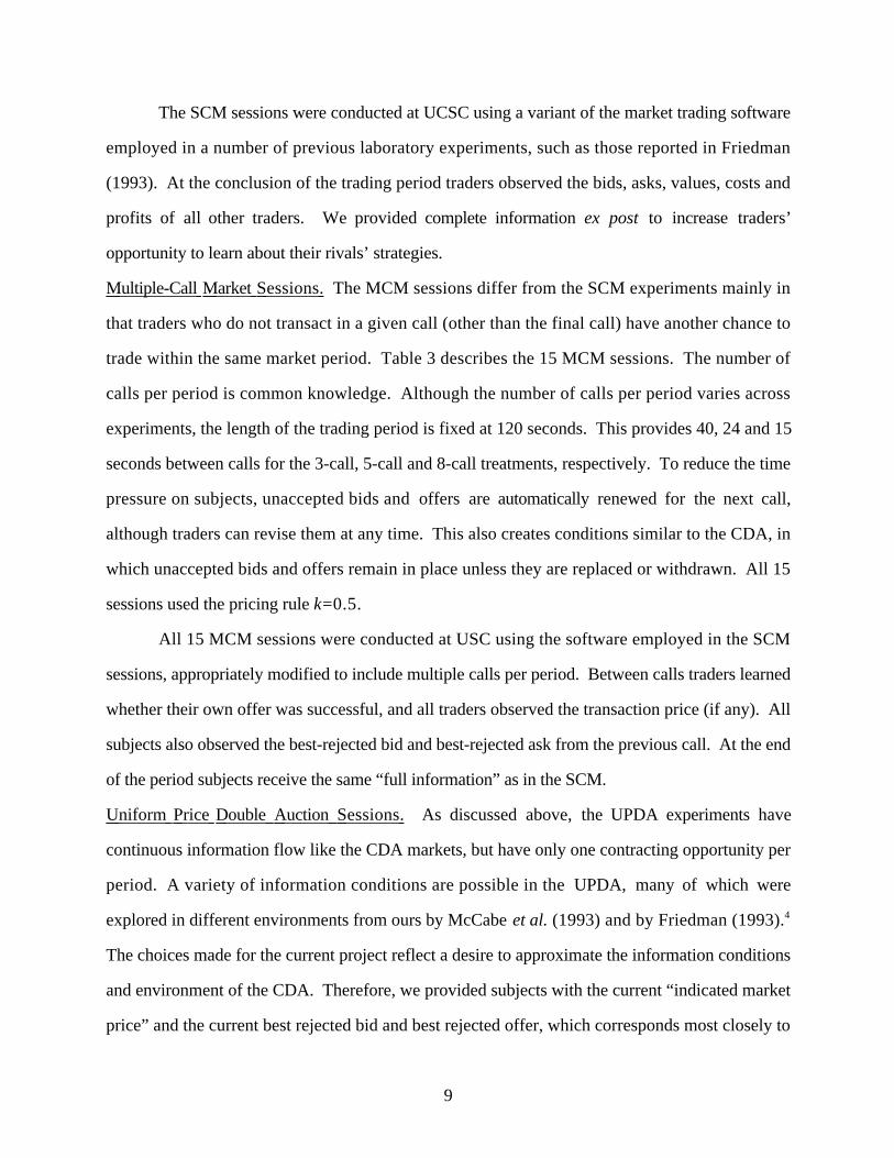
The SCM sessions were conducted at UCSC using a variant of the market trading software

employed in a number of previous laboratory experiments, such as those reported in Friedman

(1993). At the conclusion of the trading period traders observed the bids, asks, values, costs and

profits of all other traders. We provided complete information ex post to increase traders’

opportunity to learn about their rivals’ strategies.

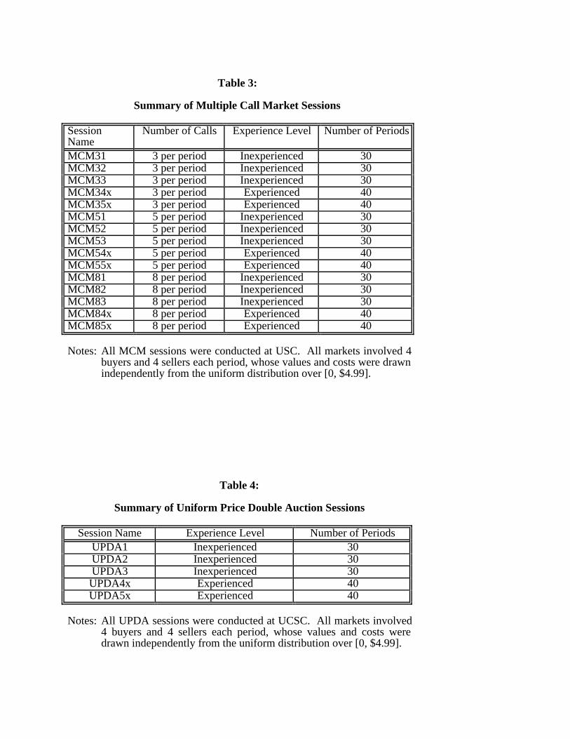
Multiple-Call Market Sessions. The MCM sessions differ from the SCM experiments mainly in

that traders who do not transact in a given call (other than the final call) have another chance to

trade within the same market period. Table 3 describes the 15 MCM sessions. The number of

calls per period is common knowledge. Although the number of calls per period varies across

experiments, the length of the trading period is fixed at 120 seconds. This provides 40, 24 and 15

seconds between calls for the 3-call, 5-call and 8-call treatments, respectively. To reduce the time

pressure on subjects, unaccepted bids and offers are automatically renewed for the next call,

although traders can revise them at any time. This also creates conditions similar to the CDA, in

which unaccepted bids and offers remain in place unless they are replaced or withdrawn. All 15

sessions used the pricing rule k=0.5.

All 15 MCM sessions were conducted at USC using the software employed in the SCM

sessions, appropriately modified to include multiple calls per period. Between calls traders learned

whether their own offer was successful, and all traders observed the transaction price (if any). All

subjects also observed the best-rejected bid and best-rejected ask from the previous call. At the end

of the period subjects receive the same “full information” as in the SCM.

Uniform Price Double Auction Sessions. As discussed above, the UPDA experiments have

continuous information flow like the CDA markets, but have only one contracting opportunity per

period. A variety of information conditions are possible in the UPDA, many of which were

explored in different environments from ours by McCabe et al. (1993) and by Friedman (1993).4

The choices made for the current project reflect a desire to approximate the information conditions

and environment of the CDA. Therefore, we provided subjects with the current “indicated market

price” and the current best rejected bid and best rejected offer, which corresponds most closely to

10

the CDA information concerning the current market bid and offer and available terms of trade.

Moreover, the sessions allow traders to cancel bids and offers (which is allowed by many

computerized CDA implementations) and calls the market after 90 seconds.5 Table 4 describes the

5 UPDA sessions, all of which were conducted at UCSC using the same market software (again

appropriately modified) that was used in the SCM and MCM sessions. Once again, traders

received complete information regarding the other traders values, costs, bids asks and profits at the

conclusion of each period, and all sessions used the pricing rule k=0.5.

4 . Results

We organize the results in 4 subsections. Section 4.1 presents example individual period

data from each institution. Section 4.2 compares the market efficiency performance across

institutions, including a decomposition of efficiency losses into two alternative sources. Section

4.3 compares realized transaction prices to the competitive equilibrium prices, and Section 4.4

compares trading volume to the competitive equilibrium volume.

4.1 Example Individual Period Data

This subsection presents a graphical description of one period for each institution--period

13 of an inexperienced session--to illustrate trader behavior and how the institutions process the

market actions (offers) into transactions. Figure 2 presents a CDA session. The right panel of the

figure presents the bids, asks and transactions for the 110 seconds of trading, and the left panel

shows the underlying values and costs for the eight traders. [Remember that these values and

costs are the same for all inexperienced sessions in period 13.] The first transaction occurs

between Seller 6 and Buyer 4 at 16 seconds. Note that Seller 6 is “extra-marginal” and should not

transact in the competitive equilibrium (CE). Because of the disequilibrium price ($3.00),

however, this is a very attractive transaction for Seller 6. Two more transactions occur later in this

period, but notice at the end Seller 7 is unable to sell a unit because of the extra-marginal

displacement of Seller 6. Trading surplus therefore falls short of the CE surplus of $7.99, but

only marginally–the difference between the costs of Seller 6 and Seller 7 ($2.08-$1.75=$0.33).

11

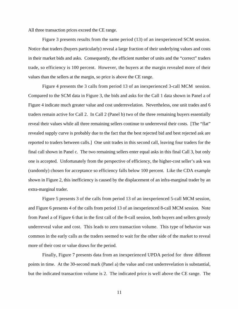
All three transaction prices exceed the CE range.

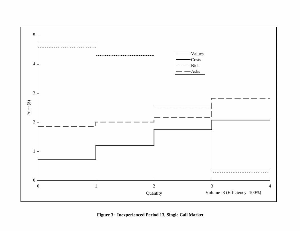
Figure 3 presents results from the same period (13) of an inexperienced SCM session.

Notice that traders (buyers particularly) reveal a large fraction of their underlying values and costs

in their market bids and asks. Consequently, the efficient number of units and the “correct” traders

trade, so efficiency is 100 percent. However, the buyers at the margin revealed more of their

values than the sellers at the margin, so price is above the CE range.

Figure 4 presents the 3 calls from period 13 of an inexperienced 3-call MCM session.

Compared to the SCM data in Figure 3, the bids and asks for the Call 1 data shown in Panel a of

Figure 4 indicate much greater value and cost underrevelation. Nevertheless, one unit trades and 6

traders remain active for Call 2. In Call 2 (Panel b) two of the three remaining buyers essentially

reveal their values while all three remaining sellers continue to underreveal their costs. [The “flat”

revealed supply curve is probably due to the fact that the best rejected bid and best rejected ask are

reported to traders between calls.] One unit trades in this second call, leaving four traders for the

final call shown in Panel c. The two remaining sellers enter equal asks in this final Call 3, but only

one is accepted. Unfortunately from the perspective of efficiency, the higher-cost seller’s ask was

(randomly) chosen for acceptance so efficiency falls below 100 percent. Like the CDA example

shown in Figure 2, this inefficiency is caused by the displacement of an infra-marginal trader by an

extra-marginal trader.

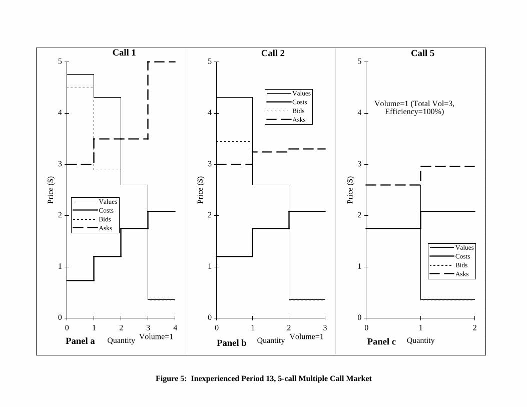
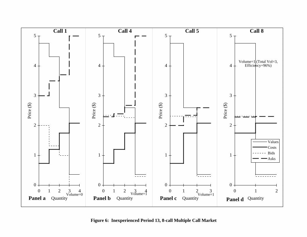
Figure 5 presents 3 of the calls from period 13 of an inexperienced 5-call MCM session,

and Figure 6 presents 4 of the calls from period 13 of an inexperienced 8-call MCM session. Note

from Panel a of Figure 6 that in the first call of the 8-call session, both buyers and sellers grossly

underreveal value and cost. This leads to zero transaction volume. This type of behavior was

common in the early calls as the traders seemed to wait for the other side of the market to reveal

more of their cost or value draws for the period.

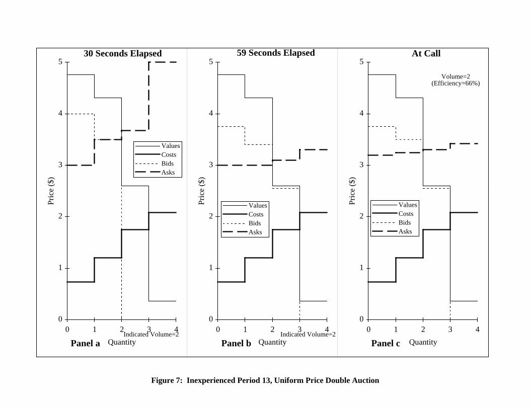
Finally, Figure 7 presents data from an inexperienced UPDA period for three different

points in time. At the 30-second mark (Panel a) the value and cost underrevelation is substantial,

but the indicated transaction volume is 2. The indicated price is well above the CE range. The

12

indicated price falls somewhat by the 59-second mark (Panel b), but is still well above the CE. At

the call (Panel c) the final value and (especially) cost underrevelation remains high, and only 2

units transact. The marginal buyer fully reveals her value, but all the sellers ask more than $3.00.

Moreover, the two highest cost sellers 6 and 7 trade, so efficiency is a dismal 66 percent. This

poor efficiency performance of UPDA is common, as we document in the next subsection.

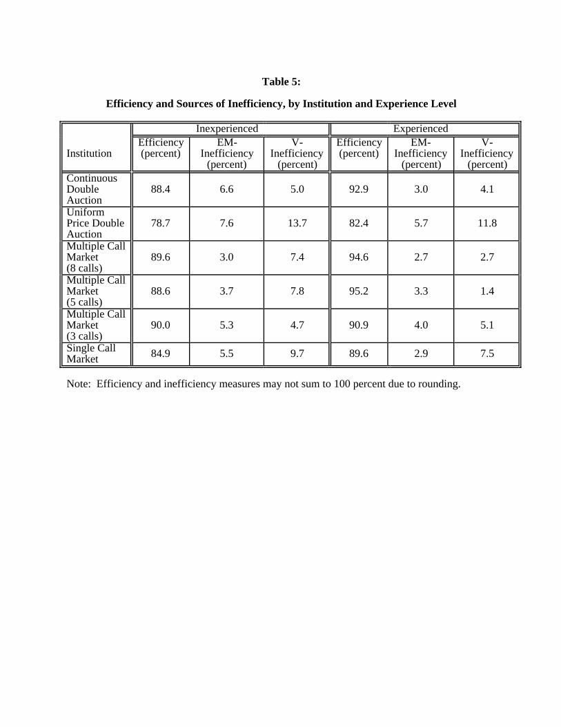
4.2 Market Trading Efficiency

Define market efficiency as the realized percentage of the maximum possible gains from

exchange. The organization of the institutions shown above in Figure 1 suggests an expected

efficiency ranking across institutions based on the two dimensions that distinguish the institutions.

If increased trading opportunities within a single period increase the extracted gains from

exchange, efficiency should increase with the number of calls in the period. Furthermore, CDA

efficiency should exceed UPDA efficiency if increased trading opportunities increase efficiency

(holding market information approximately constant). We also conjecture that increased market

information within a period improves market performance (holding trading opportunities constant).

This conjecture implies that UPDA efficiency would exceed SCM efficiency, because both

institutions permit only one trading opportunity per period but UPDA provides much more

information.

These conjectures are formally tested below using a procedure that pairs the data by period

from sessions conducted in different institutions. Recall that all sessions within an experience level

employed the same sequence of random values and costs, so this pairing by period controls for the

exogenous variation in the underlying market conditions. Although values and costs are

statistically independent across periods, idiosyncratic differences across session cohorts could

introduce some dependence across these performance measures within a session. We account for

this potential dependence using a random effects error structure for the hypothesis tests. In this

procedure the error term associated with each observation has the form eit = ui + εit, where ui is a

random session effect and εit is a standard i.i.d. error term.

13

Table 5 summarizes average efficiency for each institution, separately for inexperienced and

for experienced subjects. Our most surprising finding is that UPDA is the least efficient trading

institution in this thin volume, random values environment. This result is not due to one outlying

session; the two experienced UPDA sessions have the lowest and the third-lowest efficiency of all

the 13 experienced sessions, and the three inexperienced UPDA sessions have the lowest, second-

lowest and sixth-lowest efficiency of all the 21 inexperienced sessions. The UPDA efficiency is

significantly lower than the CDA efficiency (t-value=3.76) and is marginally significantly lower

than the SCM efficiency (t-value=1.90; p-value=0.057 for a two-tailed test). UPDA efficiency is

also significantly lower than efficiency in all three MCM treatments, with t-values ranging between

3 and 4.

We speculate that strategic misrepresentation of values and costs in the UPDA may be

causing this lower efficiency. Trader strategies are complex in this institution because of the

continuous offering opportunities, however, so it is difficult to draw clear conclusions. As one

very rough measure of the complexity of UPDA behavior, consider that the 8 subjects entered an

average of 46 market actions (offers and offer cancellations) per period in the UPDA sessions.

This far exceeds any other institution, including the CDA. We should also note that this low

UPDA efficiency is particularly surprising because McCabe et al. (1993) find that UPDA has

respectable efficiency (usually greater than 85 percent) in a random environment with additive

shifts.6 It is likely that these strategic considerations (and their negative impact on efficiency) were

increased by the thinness of the markets.

Like UPDA, the SCM has only one transaction opportunity per period and has lower

efficiency than the other institutions in both experience conditions. This provides some evidence

that multiple trading opportunities are important to generate increases in efficiency. However, the

differences between SCM efficiency and CDA and MCM efficiency are not statistically significant.

Finally, note that the MCM institution generates efficient outcomes that compare favorably with

(and are not statistically distinguishable from) the CDA outcomes, so it would appear that 3 to 5

calls per period are sufficient to generate market efficiency comparable to the CDA benchmark.

14

Efficiency can fall short of 100 percent if (a) traders with extra-marginal units transact (EM-

inefficiency), or (b) profitable trades are not executed (low volume or V-inefficiency). Table 5 also

presents the mix of V and EM inefficiency across institutions.7 Both types of inefficiency are

common, and in the inexperienced sessions shown on the left side of the table the low volume

efficiency losses exceed the extra-marginal efficiency losses in four of the six institutions. In all

institutions the increase in efficiency due to experience generally occurs because of reductions in

both types of inefficiency. In the 5-call and 8-call MCM, the reduction in V-inefficiency is quite

pronounced. For both experience conditions, low volume inefficiency is lowest for the CDA and

MCM sessions, probably due to the multiple transaction opportunities permitted by these

institutions.

4.3 Transaction Prices

The theoretical benchmark for prices across institutions is the (as-if complete information)

competitive equilibrium (CE). For this environment in nearly every period their exists a range of

CE prices where the (random) cost and value arrays overlap. Prices at any point within this CE

range have a zero deviation from the CE prediction. Average prices in a period are within the CE

range in less than one-half of the periods for all institutions. The CDA and the MCM institutions

permit multiple transaction prices per period, and theory suggests that later transaction prices in

these institutions will more accurately reflect underlying market conditions and thus “hit” the CE

more frequently than average prices. For example, most theoretical models of the CDA predict that

early transactions should occur between the highest value and lowest cost traders; see Cason and

Friedman (1993 and 1996) for some empirical evidence on this point. The final transaction prices

in each period and provide little support for this hypothesis. The CDA and MCM final transaction

prices are within the CE range only in 33 to 54 percent of the periods.

In order to provide a more formal comparison of the price performance of these

institutions, Table 6 presents the mean absolute deviation of average transaction prices (each

period) from the nearest endpoint of the CE range. [Of course, this deviation is 0 if average prices

are within the CE range.] Mean prices are closest to the CE range on average in the SCM, and are

15

farther from the CE range on average in the CDA. Statistically speaking, the CDA mean price

deviation exceeds: (1) the UPDA mean price deviation (t-value=2.33); (2) the 3-call MCM mean

price deviation (t-value=2.10); and (3) the SCM mean price deviation (t-value=3.92). The SCM

mean price deviation is also lower than the 5-call MCM mean price deviation (t-value=3.08) and

the 8-call MCM mean price deviation (t-value=2.54). The other mean price deviations are not

significantly different.

The finding here is that transaction prices differ most from the CE prediction in the CDA,

the 5-call MCM and the 8-call MCM. Mean prices deviate the least in the SCM, and the deviations

for UPDA are no greater than the mean price deviations in the MCM and CDA. This suggests that

the increase in transaction opportunities afforded by the institutions causes prices to deviate more

from the CE range. Table 6 shows that final prices differ from the CE prediction less than the

mean prices differ from the CE on average, and none of the differences in final prices deviations

are statistically significant. This indicates at least some modest convergence of prices within a

period. By aggregating all traders into a single call, however, the SCM seems to have advantages

over the other institutions on this price performance measure.

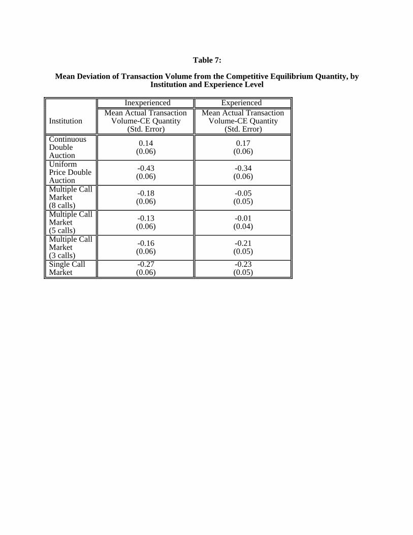
4.4 Trading Volume

Like the price performance comparison of the previous subsection, we use the CE

prediction as the theoretical benchmark. Transaction volume can exceed the CE quantity if extra-

marginal units trade due to (disequilibrium) price dispersion. Transaction volume can fall short of

the CE quantity if some subjects underreveal their true underlying value or cost, perhaps in an

attempt to manipulate prices. Either of these outcomes lead to inefficiency, and efficiency can also

fall below 100 percent even if transaction volume exactly equals to CE quantity prediction.

Table 7 presents the mean deviation of transaction volume from the CE quantity prediction,

and indicates substantial differences between the institutions. The CDA transacts the highest

volume in both experience conditions, and is significantly different from all 5 other institutions (t-

values range between 3 and 5). The UPDA volume is significantly lower than all 5 other

institutions (t-values range between 2.45 and 5.60), which is consistent with the finding in Table 5

16

that UPDA had the greatest low volume inefficiency. The SCM volume is significantly lower than

the 8-call MCM volume (t-value=2.07) and the 5-call MCM volume (t-value=2.63), but is not

significantly different from the 3-call MCM volume (t-value=0.69). The comparisons between the

different MCM treatments (i.e., 3-, 5- or 8-calls) indicate no significant differences.

Finally, note by comparing the two columns in Table 7 that trading volume (relative to the

CE prediction) increases with experience in all institutions except the 3-call MCM. This parallels

the finding in Table 5 that low volume inefficiency declines with experience in all institutions

except the 3-call MCM. Notably, in spite of this general increase in volume with increased

experience, UPDA volume in the experienced sessions falls short of the inexperienced sessions’

volume in all other institutions.

5 . Discussion

This comparison of four trading institutions in a thin market, random values environment

supports the following general conclusions. First, trading efficiency in the uniform price double

auction falls below the efficiency of the other institutions, and the single call market efficiency is no

better than any institution other than UPDA. This suggests that multiple trading opportunities

(permitted in the continuous double auction and the multiple call market) are important to generate

high efficiency. Second, the primary source of efficiency losses in these (single opportunity)

institutions is insufficient trading volume. Third, transaction prices are less accurate on average (in

that they deviate more from competitive equilibrium levels) in the continuous double auction and

multiple call market, although there is some evidence of price convergence within a period that

increases accuracy for later transactions. Taken together, these results highlight a key tradeoff

when the trading institution permits multiple transaction opportunities. Multiple transaction

opportunities substantially reduce (low volume) inefficiency due to underrevelation of traders’ true

values and costs, but also reduce pricing accuracy because traders negotiate transactions on a more

individual rather than aggregate basis.

We see the need for at least three kinds of follow-up work. First, we believe that further

17

analyses of these data at the individual subject level would provide additional insight into the

behavior of these trading institutions. These analyses should focus on specific features of

individual trader strategies, in order to compare the strategic behavior induced by the specific rules

of the alternative institutions. One measure of strategic behavior that might prove particularly

useful for this comparison is traders’ underrevelation of true values and costs, which is dependent

on time, value and other factors.

Second, we see a need for comparisons between these (and perhaps other) institutions in

thicker markets. Theory suggests that strategic incentives of these institutions become less

important as the number of traders increases, which could alter the rankings in these thin markets.

This conjecture is supported by some previous laboratory studies of these institutions in thicker

markets, often conducted with stationary values and costs. These previous studies typically find

impressive performance of all four institutions, but do not directly compare results based on

identical environments.

Third, it is time to begin the laboratory study of personalized market institutions. We have

in mind an environment where transaction cost declines over time as a buyer and seller remain

attached, but individual values and costs are subject to shocks. The institutions would vary the

technology for locating and retaining transaction partners.

Speculation on the general performance of market institutions is premature until the follow-

up work is complete, but that shall not deter us. We conjecture that a tractable theoretical model of

individual behavior will be found that adequately accounts for the observed institutional differences

in the laboratory markets. The most promising candidates, we believe, are belief learning models

(e.g., Stahl 1995; Cheung and Friedman 1995) applied to the degree of underrevelation of value

and cost. Such models will be able to predict the performance characteristics of new laboratory

market institutions in new environments and will be able to predict the performance of existing (or

new) field markets. Successful predictions would mean that the Clower and Howitt challenge is

met and the path is clear for real progress on the core issues of economics.

18

Endnotes

1Indeed, we may have a corollary at work here to Smith’s famous dictum that specialization in production is

determined by the extent of the market. The specialization of markets (time and place of delivery, and attributes of

the goods, etc.) is itself determined by the extent of the (broadly defined) market. See Friedman (1993 pp. 411-12)

for some remarks on these points, which deserve a fuller treatment.

2It is equally important to study the performance characteristics of institutions that support trade in personalized or

credence goods such as labor or financial and legal services. Indeed, Robert Clower’s vision of macrodynamics

emphasizes the interaction of such markets with the sort of auction markets we study here. See Peter Howitt’s

chapter in this volume for a simulation study of the personalized markets.

3Peter Howitt points out that high frequency MCM markets also resemble the random encounter markets of

Edgeworth because of the effective thinness at most calls.

4Among the possible information conditions are: (a) No information regarding other’s bids and asks (i.e. , essentially

the SCM); (b) Information about the current “indicated market price”; (c) Condition b plus the current best rejected

bid and best rejected offer; and, (d) Conditions b and c plus the entire current vectors of bids and offers (i.e. , an open

book). Other possible design variants include whether or not traders can withdraw previously-entered bids or offers

and the rule for determining when the market is called (e.g., at a fixed point in time or when market activity falls

below some threshold).

5In the terminology of McCabe et al. (1993) for their various UPDA treatment, we use a fixed-time (exogenous) call,

a both-sides (2s) update rule, and an information variant between their open and closed book treatments.

6Although our UPDA is implemented differently, the McCabe et al. (1993) results suggest that two design features

we employ–namely the fixed (exogenous) close and the both-sides price update rule) have a negative impact on

efficiency.

7Following the approach in Rust et al. (1993), we perform an “inefficiency audit” to decompose efficiency losses.

Assigning inefficiency to the two classes is straightforward if no extra-marginal units trade but trading volume falls

short of the efficient level (V-inefficiency), or if trading volume equals or exceeds the efficient level and efficiency is

not 100 percent (EM-inefficiency). However, if trading volume is less than the efficient level and any extra-marginal

units trade, both kinds of inefficiency are present and there is no unambiguous way to allocate losses to each class.

19

In these circumstances (which are relatively rare in the data), an extra-marginal unit has displaced an infra-marginal

unit (EM-inefficiency), and another infra-marginal unit simply fails to transact (V-inefficiency). The ambiguity

arises because we cannot identify which infra-marginal unit to assign to each class. Following Rust et al. (1993,

their appendix), we assume that each of these units is equally likely to be displaced by the extra-marginal unit, so we

compute the EM-inefficiency and V-inefficiency using the average value of the untraded infra-marginal units.

Table 1:

Summary of Continuous Double Auction Sessions

Session Name Experience Level Number of PeriodsDA441 Inexperienced 30DA442 Inexperienced 30DA443 Inexperienced 30DA443x Experienced 40DA445x Experienced 40

Notes: All CDA sessions were conducted at USC using the Multiple UnitDouble Auction (MUDA) trading program. All markets involved 4buyers and 4 sellers each period, whose values and costs were drawnindependently from the uniform distribution over [0, $4.99].

Table 2:

Summary of Single Call Market Sessions

SessionName

k Treatment Experience Level Number of Periods

k0-hum-1 k=0 Inexperienced 30k0-hum-2 k=0 Inexperienced 30k0-hum-3x k=0 Experienced 40k5-hum-6 k=0.5 Inexperienced 30k5-hum-7 k=0.5 Inexperienced 30k5-hum-8x k=0.5 Experienced 40k1-hum-11 k=1.0 Inexperienced 30k1-hum-12 k=1.0 Inexperienced 30k1-hum-13x k=1.0 Experienced 40

Notes: All SCM sessions were conducted at UCSC. All markets involved 4buyers and 4 sellers each period, whose values and costs were drawnindependently from the uniform distribution over [0, $4.99].

Table 3:

Summary of Multiple Call Market Sessions

SessionName

Number of Calls Experience Level Number of Periods

MCM31 3 per period Inexperienced 30MCM32 3 per period Inexperienced 30MCM33 3 per period Inexperienced 30MCM34x 3 per period Experienced 40MCM35x 3 per period Experienced 40MCM51 5 per period Inexperienced 30MCM52 5 per period Inexperienced 30MCM53 5 per period Inexperienced 30MCM54x 5 per period Experienced 40MCM55x 5 per period Experienced 40MCM81 8 per period Inexperienced 30MCM82 8 per period Inexperienced 30MCM83 8 per period Inexperienced 30MCM84x 8 per period Experienced 40MCM85x 8 per period Experienced 40

Notes: All MCM sessions were conducted at USC. All markets involved 4buyers and 4 sellers each period, whose values and costs were drawnindependently from the uniform distribution over [0, $4.99].

Table 4:

Summary of Uniform Price Double Auction Sessions

Session Name Experience Level Number of PeriodsUPDA1 Inexperienced 30UPDA2 Inexperienced 30UPDA3 Inexperienced 30UPDA4x Experienced 40UPDA5x Experienced 40

Notes: All UPDA sessions were conducted at UCSC. All markets involved4 buyers and 4 sellers each period, whose values and costs weredrawn independently from the uniform distribution over [0, $4.99].

Table 5:

Efficiency and Sources of Inefficiency, by Institution and Experience Level

Inexperienced Experienced

InstitutionEfficiency(percent)

EM-Inefficiency

(percent)

V-Inefficiency

(percent)

Efficiency(percent)

EM-Inefficiency

(percent)

V-Inefficiency

(percent)ContinuousDoubleAuction

88.4 6.6 5.0 92.9 3.0 4.1

UniformPrice DoubleAuction

78.7 7.6 13.7 82.4 5.7 11.8

Multiple CallMarket(8 calls)

89.6 3.0 7.4 94.6 2.7 2.7

Multiple CallMarket(5 calls)

88.6 3.7 7.8 95.2 3.3 1.4

Multiple CallMarket(3 calls)

90.0 5.3 4.7 90.9 4.0 5.1

Single CallMarket 84.9 5.5 9.7 89.6 2.9 7.5

Note: Efficiency and inefficiency measures may not sum to 100 percent due to rounding.

Table 6:

Mean Absolute Deviation of Transaction Prices (in Cents) from the CompetitiveEquilibrium Price Interval, by Institution and Experience Level

Inexperienced Experienced

InstitutionMean Prices(Std. Error)

Final PricesEach Period(Std. Error)

Mean Prices(Std. Error)

Final PricesEach Period(Std. Error)

ContinuousDoubleAuction

0.27(0.04)

0.24(0.04)

0.23(0.03)

0.18(0.03)

UniformPrice DoubleAuction

0.20(0.03)

(same asmean price)

0.19(0.03)

(same asmean price)

Multiple CallMarket(8 calls)

0.26(0.03)

0.23(0.04)

0.19(0.03)

0.13(0.03)

Multiple CallMarket(5 calls)

0.30(0.04)

0.27(0.05)

0.18(0.03)

0.13(0.03)

Multiple CallMarket(3 calls)

0.20(0.03)

0.20(0.03)

0.20(0.04)

0.18(0.04)

Single CallMarket

0.18(0.03)

(same asmean price)

0.11(0.02)

(same asmean price)

Table 7:

Mean Deviation of Transaction Volume from the Competitive Equilibrium Quantity, byInstitution and Experience Level

Inexperienced Experienced

InstitutionMean Actual Transaction

Volume-CE Quantity(Std. Error)

Mean Actual TransactionVolume-CE Quantity

(Std. Error)ContinuousDoubleAuction

0.14(0.06)

0.17(0.06)

UniformPrice DoubleAuction

-0.43(0.06)

-0.34(0.06)

Multiple CallMarket(8 calls)

-0.18(0.06)

-0.05(0.05)

Multiple CallMarket(5 calls)

-0.13(0.06)

-0.01(0.04)

Multiple CallMarket(3 calls)

-0.16(0.06)

-0.21(0.05)

Single CallMarket

-0.27(0.06)

-0.23(0.05)

ContinuousDoubleAuction(CDA)

Single-Call

Market(SCM)

8Calls

5Calls

3Calls

UniformPrice

DoubleAuction(UPDA)

Trading Opportunities Dimension

Information Dimension

Figure 1: An Overview of the Trading Institution Comparison and Experimental Design

Multiple-Call Market (MCM)

Within-periodInformation Held

(Approx.) Constant

TradingOpportunitiesHeld Constant

0

1

2

3

4

5

0 1 2 3 4

Quantity

Pric

e ($

)

ValuesCosts

Values and CostsBuyer 4

Buyer 3

Buyer 2

Buyer 1Seller 8

Seller 5

Seller 7

Seller 6

Panel a

(CE Price Range [1.75, 2.08])

(CE Quantity=3)

(CE Surplus=7.99)

0

1

2

3

4

5

0 10 20 30 40 50 60 70 80 90 100 110

Seconds in Period

Pric

e ($

)

BidsAsks

Bids and Asks

Volume=3 (Efficiency=96%)

S6

B2

B3

S5 S6

B4S6 accepts B4

S8

B2

S7

B2

S8 S7

S8 accepts B2

B3

S7

B3S5 accepts B3

S7

Panel b

Figure 2: Inexperienced Period 13, Continuous Double Auction

0

1

2

3

4

5

0 1 2 3 4

Quantity

Pric

e ($

)

ValuesCostsBidsAsks

Volume=3 (Efficiency=100%)

Figure 3: Inexperienced Period 13, Single Call Market

0

1

2

3

4

5

0 1 2 3 4

Quantity

Pric

e ($

)

ValuesCostsBidsAsks

Call 1

Volume=1Panel a

0

1

2

3

4

5

0 1 2 3

Quantity

Pric

e ($

)

ValuesCostsBidsAsks

Call 2

Volume=1Panel b

0

1

2

3

4

5

0 1 2

QuantityPr

ice

($)

ValuesCostsBidsAsks

Call 3

Volume=1 (Total Vol=3, Efficiency=89%)

Panel c

Figure 4: Inexperienced Period 13, 3-call Multiple Call Market

0

1

2

3

4

5

0 1 2 3 4

Quantity

Pric

e ($

)

ValuesCostsBidsAsks

Call 1

Volume=1Panel a

0

1

2

3

4

5

0 1 2 3

Quantity

Pric

e ($

)

ValuesCostsBidsAsks

Call 2

Volume=1Panel b

0

1

2

3

4

5

0 1 2

QuantityPr

ice

($)

ValuesCostsBidsAsks

Call 5

Volume=1 (Total Vol=3, Efficiency=100%)

Panel c

Figure 5: Inexperienced Period 13, 5-call Multiple Call Market

0

1

2

3

4

5

0 1 2 3 4

Quantity

Pric

e ($

)Call 1

Volume=0Panel a

0

1

2

3

4

5

0 1 2 3 4

Quantity

Pric

e ($

)

Call 4

Volume=1Panel b

0

1

2

3

4

5

0 1 2 3

Quantity

Pric

e ($

)

Call 5

Volume=1Panel c

0

1

2

3

4

5

0 1 2

Quantity

Pric

e ($

)

Values

Costs

Bids

Asks

Call 8

Volume=1 (Total Vol=3, Efficiency=96%)

Panel d

Figure 6: Inexperienced Period 13, 8-call Multiple Call Market

0

1

2

3

4

5

0 1 2 3 4

Quantity

Pric

e ($

)

ValuesCostsBidsAsks

30 Seconds Elapsed

Indicated Volume=2

Panel a

0

1

2

3

4

5

0 1 2 3 4

Quantity

Pric

e ($

)ValuesCostsBidsAsks

59 Seconds Elapsed

Indicated Volume=2

Panel b

0

1

2

3

4

5

0 1 2 3 4

QuantityPr

ice

($)

ValuesCostsBidsAsks

At Call

Volume=2(Efficiency=66%)

Panel c

Figure 7: Inexperienced Period 13, Uniform Price Double Auction

References

Affleck-Graves, J., S. Hedge and R. Miller (1994), “Trading Mechanisms and the Components ofthe Bid-Ask Spread,” Journal of Finance 49, pp. 1471-1488.

Arrow, K. and Hahn, F. (1972), General Competitive Analysis (Holden-Day, San Francisco).

Arrow, K. and L. Hurwicz (1958), “On the Stability of Competitive Equilibrium I,” Econometrica26, pp. 522-552.

Cason, T. and D. Friedman (1993), “An empirical analysis of price formation in double auctionmarkets,” in: D. Friedman and J. Rust, eds., The Double Auction Market (Addison-Wesley, Reading, MA), pp. 253-283.

Cason, T. and D. Friedman (1996), “Price Formation in Double Auction Markets,” Journal ofEconomic Dynamics and Control, forthcoming.

Cason, T. and D. Friedman (1997), “Price Formation in Single Call Markets,” Econometrica,forthcoming.

Cheung, Y.-W. and D. Friedman (1995), “Individual Learning in Games: Some LaboratoryResults,” Manuscript, University of California at Santa Cruz Department of Economics.

Clower, R. (1959), “Some Theory of an Ignorant Monopolist,” Economic Journal 69, pp. 705-716.

Clower, R. (1975), “Reflections on the Keynesian Perplex,” Zeitschrift für Nationalokonomie 35,pp. 1-24.

Clower, R. (1977), “The Anatomy of monetary theory,” American Economic Review Papers andProceedings 67, pp. 206-212.

Clower, R. (1990), “The Monetary Economics of John Hicks,” Greek Economic Review 12(supplement), pp. 73-84.

Clower, R. and P. Howitt (1996), “Taking Markets Seriously,” in: D. Colander, ed., BeyondMicrofoundations: Post-Walrasian Macroeconomics (Cambridge Univ. Press, Cambridge),pp. 21-37.

Easley, D. and J. O. Ledyard (1993), “Theories of price formation and exchange in double oralauctions,” in: D. Friedman and J. Rust, eds., The Double Auction Market (Addison-Wesley, Reading, MA), pp. 63-97.

Friedman, D. (1979), “Money-Mediated Disequilibrium Processes in a Pure Exchange Economy,”Journal of Mathematical Economics 6, pp. 149-167.

Friedman, D. (1991a), “A Simple Testable Model of Double Auction Markets,” Journal ofEconomic Behavior and Organization 15, pp. 47-70.

Friedman, D. (1991b), “Evolutionary Games in Economics,” Econometrica 59, pp. 637-666.

Friedman, D. (1993), “How trading institutions affect financial market performance: Somelaboratory evidence,” Economic Inquiry 31 pp. 410-435.

Friedman, D. and J. Ostroy (1995), “Competitivity in auction markets: An experimental andtheoretical investigation,” Economic Journal 105, pp. 22-53.

Gale, D. (1987), “Limit Theorems for markets with sequential bargaining,” Journal of EconomicTheory, pp. 20-54.

Gode, D. K. and S. Sunder (1993), “Allocative efficiency of markets with zero intelligence (ZI)traders: Market as a partial substitute for individual rationality,” Journal of PoliticalEconomy 101, pp. 119-137.

Hicks, J. (1939), Value and Capital, Oxford: Oxford University Press.

Ho, T. and Stoll, H. (1983), “The Dynamics of Dealer Markets Under Competition,” The Journalof Finance, pp. 1053-1074.

Kagel, J. H. (1994), “Double auction markets with stochastic supply and demand schedules: Callmarkets and continuous auction trading mechanisms,” Manuscript, University ofPittsburgh Department of Economics.

Kagel, J. H., and W. Vogt (1993), “The Buyers Bid Double Auction: Preliminary ExperimentalResults,” in: D. Friedman and J. Rust, eds., The Double Auction Market (Addison-Wesley, Reading, MA), pp. 285-305.

Kiyotaki, N. and R. Wright (1989), “On Money as the Medium of Exchange,” Journal of PoliticalEconomy 97, pp. 927-54.

McCabe, K., S. Rassenti and V. Smith (1993), “Designing a Uniform Price Double Auction: AnExperimental Evaluation,” in: D. Friedman and J. Rust, eds., The Double Auction Market(Addison-Wesley, Reading, MA), pp. 307-332.

O’Hara, M. (1995), Market Microstructure Theory (Basil Blackwell, Cambridge, Mass.).

Okun, A. (1981), Prices and Quantities: A Macroeconomic Analysis (Brookings Institution,Washington DC).

Plott, C. (1991), “A computerized laboratory market system and research support systems for themultiple unit double auction,” Social Science Working Paper 783, California Institute ofTechnology.

Rust, J., R. Palmer and J. Miller (1993), “Behavior of trading automata in a computerized doubleauction market,” in: D. Friedman and J. Rust, eds., The Double Auction Market (Addison-Wesley, Reading, MA), pp. 155-198.

Rustichini, A., M. Satterthwaite and S. Williams (1994), “Convergence to Efficiency in a SimpleMarket with Incomplete Information,” Econometrica 62, 1041-1063.

Samuelson, P. (1948), Foundations of Economic Analysis, (Harvard University Press,Cambridge, MA).

Satterthwaite, M. and S. Williams (1993), “The Bayesian Theory of the k-Double Auction,” in: D.Friedman and J. Rust, eds., The Double Auction Market (Addison-Wesley, Reading, MA),pp. 99-123.

Schecter, S. (1975), “Smooth Pareto Economic Systems with Natural Boundary Conditions,”Ph.D. Thesis, University of California, Berkeley.

Smale, S. (1976), “Exchange Processes with Price Adjustment,” Journal of MathematicalEconomics 3, pp. 211-226.

Smith, V., A. Williams, W. K. Bratton and M. Vannoni (1982), “Competitive Market Institutions:Double Auctions vs. Sealed Bid-Offer Auctions,” American Economic Review 72, pp. 58-77.

Stahl, D. (1995), “Evidenced Based Rule Learning in Symmetric Normal-Form Games,”Manuscript, University of Texas Department of Economics.

Stoll, H. R. and R. E. Whaley (1990), “Stock market structure and volatility,” Review ofFinancial Studies 3, pp. 37-71.

Walras, L. (1973), Elements of Pure Economics, translated by W. Jaffe (Irwin Press,Homewood, IL) (original version published 1874).

Wan, Y. (1980), “On Disequilibrium Adjustment Processes,” Journal of Mathematical Economics7, pp. 151-163.

Wilson, R. (1987), “On equilibria of bid-ask markets,” in: G. Feiwel, ed., Arrow and the Ascentof Modern Economic Theory (The MacMillan Press Ltd., Houndmills, UK), pp. 375-414.

Wollinsky, A. (1990), “Information revelation in a market with pairwise meetings,” Econometrica58, pp. 1-23.