Price Instability, Exchange Rate Volatility and the ...

Journal of Economics and Sustainable Development www.iiste.org

ISSN 2222-1700 (Paper) ISSN 2222-2855 (Online)

Vol.7, No.4, 2016

89

Price Instability, Exchange Rate Volatility and the Nigerian

Economy: An Empirical Analysis

Folorunso Sunday Ayadi* Olajide Anuoluwa Jeremiah

Economics Department, Faculty of Social Sciences, University of Lagos, Nigeria

Abstract

Previous studies on price and exchange rate volatility have commonly focused on its effect on FDI and some

sectors of the Nigerian economy, and not much has been conducted on its effect on the economy as a whole. This

research therefore empirically verified the dynamics of price and exchange rate volatility on the Nigerian

economy for the period of 1970 to 2010. The study was conducted by building a model which looked at the

relationship between price, exchange rate and economic growth. Exchange rate variability was estimated using

the GARCH model and variables were tested for unit root (stationarity). Consequently, the Johansen

cointegration test was also conducted. The analysis was concluded with the estimation of the Error Correction

Model (ECM) and interpretation of the short-run and long-run (OLS) results. The study found that the exchange

rate in Nigeria is volatile, as the trend shows the fluctuation in price and exchange rate which of course may bear

serious implications. Their instability however did not discourage investment and consequently economic growth

both in the short and long run. Based on the regression result, it was observed that 1% change in money supply

led to about 83.2% change in RGDP, the implication of this is that monetary variable may be a reliable

instrument of ensuring growth in the long run. In addition, trade openness significantly depresses growth in the

short and long run suggesting the adoption of inward growth strategy.

Keywords: Exchange rate, Growth, Inflation, Macroeconomics, Trade openness.

1. Introduction

There has been an ongoing debate about the appropriate exchange rate policy in developing countries. The

debate focuses on the degree of fluctuations in the exchange rate in the face of internal and external shocks.

Exchange rate fluctuations are likely, in turn, to determine economic performance. In judging the desirability of

exchange rate fluctuations, it become, therefore, necessary to evaluate their effects on output growth and

inflation via the demand and supply channels. A depreciation (or devaluation) of the domestic currency may

stimulate economic activity through the initial increase in the price of foreign goods relative to home goods. By

increasing the international competitiveness of domestic industries, exchange rate depreciation may divert

spending from foreign goods to domestic goods.

Hirschman (1949) points out that currency depreciation from an initial trade deficit reduces real national income

and may lead to a fall in aggregate demand. In other words, currency depreciation gives with one hand, by

lowering export prices, while taking away with the other hand, by raising import prices. If trade is in balance and

terms of trade are not changed, these price changes offset each other. But if imports exceed exports, the net result

is a reduction in real income within the country. Cooper (1971) also confirmed this point in his general

equilibrium model. Depreciation may raise the windfall profits in export and import-competing industries. If

money wages lag, the price increases and if the marginal propensity to save from profits is higher than from

wages, national savings will go up and real output will decrease. Krugman and Taylor (1978) and Barbone and

Rivera-Batiz (1987) have formalized the same views.

Supply-side channels further complicate the effects of currency depreciation on economic performance. Bruno

(1979) and van Wijnbergen (1989) postulated that in a typical semi-industrialized country where inputs for

manufacturing are largely imported and cannot be easily produced domestically, firms’ input cost will increase

following devaluation. As a result, the negative impact from the higher cost of imported inputs may dominate the

production stimulus from lower relative prices for domestically traded goods.

Currency devaluation was bound to generate inflationary pressures as most of the imported goods had no close

domestic substitute. On one hand, it has been recognized in the literature that depreciation of exchange rate tends

to expand exports and reduce imports, while the appreciation of exchange rate would discourage exports and

encourage imports. Thus, exchange rate depreciation leads to income transfer from importing countries to

exporting countries through a shift in the terms of trade, and this affects the economic growth of both importing

and exporting nations.



Vol.7, No.4, 2016

90

Currently, economists seem to agree that high rates of inflation cause “problems” not just for some individuals,

but for aggregate economic performance. However, much less agreement exists about the precise relationship

between inflation and economic performance, and the mechanism by which inflation affects economic activity.

There exists also some evidence which strongly supports the view that the relationship between inflation and

economic growth is non-linear. Further investigation suggests that developing countries and developed countries

show different forms of non-linearity in the inflation-growth relationship.

Barro (1996) emphasize that the growing interest on price stability as a major goal of monetary policy has been

borne out by recent developments in economic literature, which tends to show that a reduction in the inflation

rate impacts measurably and positively on economic growth. Furthermore another strands of these economic

thoughts as explained by Bruno and Easterly (1996) and Mishkin and Posen (1997) imply that there is no long-

run trade-off between inflation and economic growth. Put differently, increases in economic activities can occur

without a spell of inflationary pressure as envisaged by the Phillips curve hypothesis.

In effect recent papers by some economists have demonstrated that inflation had positive effect on growth while

some other economists who are advocate of the efficient firm’s hypothesis, are preaching an inverse correlation

between inflation and economic growth. The problem therefore lies in determining the inflation rate consistent

with development and identifying the price rise that reflects inflationary pressure on the economy.

Although, there exists numerous research on separate impact of exchange rate on growth, and inflation on

growth in Nigeria (for example, Ikhide and Yinusa, 1998; Ajibefun and Daramola, 2003; Odusola and Akinlo,

2001), this approach differs in terms of methodology and focus. Thus, this study on the Nigerian economy

attempts to find out how these two macroeconomic variables interact with the economic performance. The

general objective of this study is to examine empirically the dynamics of inflation and exchange rate volatility on

the performance of Nigerian economy. This paper is divided into six sections, section 2 review relevant literature

while section 3 focuses on theoretical framework. Section 4 presents methodology and data, section 5 presents

results while the sixth section recommends.

2. Literature Review

Nwankwo (1982) defines inflation, as “excess of demand over supply at current prices. Inflation is also a

situation whereby too much money is chasing too few goods. From the definitions, it is clear that inflation has

four essential characteristics. One is increase in demand which simultaneously results in a proportionate or

higher increase in supply. If increases in demand must lead to inflation then there must also be a second factor

which is limitation of supply. But a limitation of supply will not necessarily lead to inflation unless the third

factor is present. This is an increase in the supply of money. It is this which will make the increase in demand

effective. Even then there would still be no inflation unless there is a struggle in the community for the limited

supply of goods and services. This is the fourth element. From the above four essentials of inflation, Onitiri and

Awosika (1982) defined inflation as a state of disequilibrium in which the community is struggling to acquire

more goods and services than are available and which lead to persistently rising prices.

Hashim and Zarma (1996) emphasized that exchange rate is an important economic variable as its appreciation

or depreciation affects the performance of other macroeconomic variables in any economy. Its value can be used

to assess overall performance of an economy and a very important variable in policy decision-making of an

economy. Any government at any point in time seek the stability of the exchange rate because it provides

economic agents the opportunity to plan ahead without fear of varying costs and prices of goods and services. On

the other hand, instability of exchange rate can cause a negative distortion in any economy.

Sanusi (2004) highlighted that the country’s (Nigeria’s) exchange rate policy has been aimed at preserving the

external value of the domestic currency and maintaining a healthy balance of payments position, which indeed is

a major provision of the enabling law. The problem of foreign exchange market, which Nigeria is facing just like

any other developing countries, has much to do with the gap that exists between supply of foreign exchange and

its demand. The failure of the economy to supply enough foreign exchange to meet the demand forced the

government to resort to rationing the available foreign exchange and this led to speculative hoarding and the

development of a parallel market. All these cause the instability of the exchange rate in Nigeria.

Broadly, Nigeria had adopted two exchange rate systems, the fixed and flexible exchange rate system (Hashim

and Zarma, 1996). Ogunleye (2010) noted that the real exchange rate in Nigeria has been principally influenced

by external shocks resulting from the vagaries of world price of agricultural commodities and oil price, (both

major sources of Nigerian export and foreign exchange earnings) contending that when the economy depended

on agricultural exports, real exchange rate volatility was less pronounced given the fact that these products were



Vol.7, No.4, 2016

91

subjected to less volatility, and that there were more trading partners’ currencies involved in the calculation of

the country’s real exchange rate. This to him minimally affected the real exchange rate fluctuations between

1970 and 1977.

Iyoha and Oriakhi (2002) observed that the important factor that determined the movement in real exchange rate

during the 1970's was nominal shock resulting from fiscal deficits. Ogunleye (2008) observed further that the oil

windfalls which resulted in excessive fiscal expenditure in ambitious development projects in the 1970's, forced

the government to finance its expenditures through money creation when the windfall ended. This expansionary

monetary policy exerted upward pressure on inflation, thus further aggravating sharp movements in real

exchange rate.

Adeyeye and Fakiyesi (1980), Osakwe (1993) have sought explanations for the worrisome trend in inflation in

Nigeria. Popular among the adduced reasons for the price fluctuation includes large fiscal deficits financed by

accommodating monetary policies, entrenched inflationary expectations, nominal exchange rate depreciation,

capital inflows and real factors, like drought, OPEC reduction of quota, ethnic violence and civil strife, etc. In

explaining the effect and determinants of inflation in Nigeria, other various empirical studies have been carried

out explaining this unprecedented increase in the general price level. Economists have applied more of the

combination of the monetarist’s theory and the structuralist views on inflation to explain the causes and effects of

inflation in Nigeria (Akinnifesi, 1977; Adeyeye and Fakiyesi, 1980; 1996; Egwaikhile et. al., 1994 among

others).

The connection between exchange rate variability and inflation has been explained by Hyder and Shah (2004).

Exchange rate movement can influence domestic prices via their effect on aggregate supply and demand. On the

supply side, exchange rate could affect prices paid by the domestic buyers of imported goods directly. In an open

economy, when the currency depreciates, it will result in higher import prices and vice versa. Exchange rate

fluctuations could have an indirect supply effect on domestic prices. The potentially higher cost of imported

inputs associated with an exchange rate depreciation increases marginal cost and lead to higher prices of

domestically produced goods. Furthermore, import-competing firms might increase prices in response to an

increase in foreign competitor’s price in order to improve profit margins. The extent of such price adjustment

depends on a variety of factors such as market structure, nature of government, exchange rate policy, or product

substitutability. While on the demand side, exchange rate depreciation (appreciation) increases (decreases)

foreign demand for domestic goods and services, causing increase (decrease) in net export and hence aggregate

demand (see also Rosenberg, 2003).

A relatively large number of studies have attempted to estimate the impact of price and exchange rate variation

on economic performance using various methodologies. Agénor (1991) using a sample of twenty-three

developing countries, regressed output growth on contemporaneous and lagged levels of the real exchange rate

and on deviations of actual changes from expected ones in the real exchange rate, government spending, the

money supply, and foreign income. The results showed that surprises in real exchange rate depreciation actually

boosted output growth, but that depreciations of the level of the real exchange rate exerted a contractionary effect

on growth.

Hasanov (2011) examined the possibility of threshold effect of inflation on economic growth over the period of

2000-2009. Estimated threshold model indicated that there is a non-linear relationship between economic growth

and inflation in the Azerbaijani economy and threshold level of inflation for GDP growth is 13 percent. Below

threshold level, inflation has statistically significant positive effect on GDP growth, but this positive relationship

becomes negative one when inflation exceeds 13 percent. Also, Grimes (1991) analyzed data of 21 countries

covering 1961-1987, and found a positive relationship between inflation and economic growth for a short term,

and a negative relationship between them for a long term.

Ghosh, et. al. (1997) points to inflation volatility as being, at least, as important as average inflation. The authors

analyzed 140 countries over a 30-year period, and divided them into 9 groups according to their exchange rate

regime. Then, they regressed inflation volatility against the Central Bank’s turnover rate, degree of openness,

volatilities of output growth and of money supply and interest rates, plus dummies for fixed and intermediate

exchange rate regimes. However, when they split the countries into groups, results show that inflation volatility

is lower under the floating and intermediate exchange rate regime for countries with low inflation.

Petreski (2009) conducted a literature review on the relationship between exchange rate regime and growth with

the aim of examining the theoretical and empirical arguments for the relationship. He found that as a nominal

variable, exchange rate may not impact on the long –run growth process. He further concluded that there is

ambiguous theoretical evidence of the effect the exchange rate target have on economic growth. The channel

through which exchange rate impacts growth is trade, investment and productivity. In addition, theoretical



Vol.7, No.4, 2016

92

considerations link exchange-rate effect on growth to the uncertainty level caused by the flexible option of the

rate. However, the relationship remains controversial theoretically requiring empirical analysis. The empirical

research remains divergent. On the overall, these empirical works have the following shortcomings. The growth-

framework used not appropriate, problem of endogeniety (exchange rate and growth), sample selection bias

among others.

Stotsky et. al. (2012) examines the relationship between foreign exchange regime and macroeconomic

performance in seven East African countries with 5 of which foreign exchange regimes are liberalized using the

generalized method of moment. They developed two models, one which relates growth and its determinants

which include inflation, nominal exchange rate and liberalization among others. The other model relates inflation

to its various determinants which include lagged inflation, exchange rate and liberalization among others. They

found that investment and real exchange rate are the significant determinants of growth while the lagged

inflation rate, nominal exchange rate and de facto regime are the significant determinants of inflation. The cue

we take from the growth model is that if the real exchange rate influences growth, what impact the exchange rate

volatility would have on growth is worth an effort.

Harms and Kreschmann (2009) conducted a study on some developing countries to investigate the relationship

between exchange rate regime and growth and they found out that less flexible regimes confers some benefits in

the sampled countries. However, when inflation is taken into consideration by removing high inflation periods

from the sample, the benefits disappear. This implies that inflation distorts the impact of exchange rate growth.

Okhiria and Saliu (2008) employed econometric techniques to investigate the impact of currency devaluation on

output growth and inflation rate and they found that devaluations (either increases in the level of the real

exchange rate or in the rate of depreciation) were associated with a reduction in output and increase in inflation.

Cooper (1971) reviewed twenty-four devaluation experiences involving nineteen different developing countries

during the period 1959–66. The study showed that devaluation improved the trade balance of the devaluing

country but that the economic activity often decreased in addition to an increase in inflation in the short term.

On this debate, the conclusion of Du and Zhu (2001) is relevant. They posited that results from many empirical

studies differ from country to country even, when the same method of examination is applied. It also differs for

same country at different point of time. Survey of literature showed that the debate on growth, exchange rate and

inflation is still fraught with considerable controversy. In addition few researches have been done on the

combined role of inflation and exchange rate variability and economic growth. So, additional research in this

area is still of importance.

3. Theoretical Framework

The link between exchange rate, inflation and economic growth is better explained using the Balassa-Samuelson

model (B-S model) which is presented using a single-factor aggregate production function of Obstfeld and

Rogoff (1996). This model assumes that the production functions of tradable (T) and non-tradable goods (N)

take the following form:

where Y is production, A is a constant describing technology, and L is labor force. Foreign economies employ

the same kind of technology as the domestic economy, but may differ from it in the value of the technological

parameter A; the subscript T denotes the tradable sector, and the subscript N is the non-tradable sector. This

model also assumes that the law of one price holds for tradable commodities and that the world price of tradable

commodities is equal to one without a loss of generality. In addition, perfect labor mobility is assumed between

sectors within an individual economy, but zero mobility of labor is assumed between economies. The mobility of

labor insures that the wage rates w are equal in other sectors of the same economy. We define the price index as

the weighted geometric average of prices of tradable and non-tradable goods as:



Vol.7, No.4, 2016

93

, where is the share of tradable

goods in total outputs. If this share is the same at home as abroad, the relative price vis-a-vis the outside world is

expressed as

, and the nominal GDP per employee is expressed as

the relative price can then be transformed into

This formula states that the relative price is determined by relative GDP and the relative technological level or

productivity in non-tradable sector of the two economies. Given a level of productivity at home and abroad, a

higher nominal GDP growth at home than abroad leads to an appreciation of the real exchange rate. On the other

side, given an economic growth rate, higher productivity of non-tradables in the home country than the foreign

country will lead to depreciation of the real exchange rate.

This simplified model can be easily extended to a more general one that includes two production factors: labor

and capital. Let us consider a small economy that produces two composite goods: tradables and non-tradables.

We assume that the production functions are functions of capital and labor with constant return to scale:

where K denotes capital. The other variables are the same as above. Through some manipulation, the log-

differentiation of the relative price of tradable goods and non-tradable goods can be expressed as

where and are respectively the labor share of the

income generated in the tradable and non-tradable goods sectors.

Provided that non-tradables are relatively labor intensive, meaning

, the model forecasts that the domestic economy will experience real appreciation if its

productivity-growth advantage in tradables exceeds its productivity growth advantage in non-tradables.

The Balassa-Samuelson model is one of the cornerstones of the traditional theory of the real equilibrium

exchange rate. The key empirical observation underlying the model is that countries with higher productivity in

tradables compared with non-tradables tend to have high price levels. The B-S model hypothesis states that

productivity gains in the tradable sector allow real wages to increase commensurately and, since wages are



Vol.7, No.4, 2016

94

assumed to link the tradable to the non-tradable sector, wages and prices also increase in the non-tradable sector,

leading to an increase in the overall price level in the economy, which in turn results in an appreciation of the

real exchange rate.

4. Methodology and Data

The model employed in this study is hereunder stated:

GDP= f(INF,M2,OPNS,INT, EXCVL) (1)

logGDP= β0+ β1INF+ β2 logM2+ β3OPNS+ β4INT+ β5EXCVL+ Ut (2)

Where ß0, ß1, ß2, ß3, ß4, and ß5 are parameters of the model, exchange rate volatility (EXCVL), inflation rate

(INFL), broad money supply (M2), trade openness (OPNS) and Interest Rate (INT) respectively; Ut is the

disturbance term.

Trade openness (OPNS) is calculated as (Total Trade/GDP), while exchange rate volatility (EXVL) would be

measured with the use of GARCH in order to determine how volatile the exchange rate has been over the years.

4.1 Estimation Techniques

Although time series data are used in many econometric studies, they present some special problems for

econometricians. Most of the empirical work based on time series data assumes that the underlying time series

are stationary. In regressing a non-stationary time series variable on another, one often obtains a very high

coefficient of determination (R²) although there is no meaningful relationship between the two. This is the

problem of spurious regression. This problem arises because if both the time series involved exhibit strong trends

(sustained upward or downward movements), the high coefficient of determination (R²) observed is due to the

presence of the trend, and not because of a true relationship between the two variables.

Any time series can be thought of as being generated by a stochastic or random process. A stochastic process is

said to be stationary if its mean and variance are constant over time and the value of covariance between two

time periods depends only on the distance or lag between two time periods and not on the actual time at which

the covariance is computed. An alternative test of stationary that has become popular is known as unit root test.

This study would however utilize the Augmented Dickey Fuller (ADF) method to test for the stationarity of the

variables. Most macroeconomic time series have unit roots and regressing non-stationary data against another is

bound to yield spurious regression result. We conducted a unit root test and based on the order of integration

conducted Johansen cointegration test which indicates the presence of cointegrating equation. Meaning that even

though variables are non stationary at levels, a combination of nonstationary variables can produced a stationary

result. We went further by estimating the error correction model and the static model

The data that employed in this research work are secondary in nature. They are gotten from various issues of the

Central Bank of Nigeria Statistical Bulletin and National Bureau of Statistics, whom which reliance is total in the

case of data sourcing in Nigeria. The data ranges from 1970 through 2010.

5. Results Presentation

The exchange rate volatility in Nigeria from 1970-2010 was obtained through the estimation of Autoregressive

Conditional Heteroscedasticity {ARCH} and Generalized Autoregressive Conditional Heteroscedasticity

{GARCH (1,1)} model. It can be seen from the graph that the trend of exchange rate volatility grew sharply

between 1971-1977, and a steady growth between1978-1999 where it experienced a minimal volatility within the

range of 197.94 and 200.31, but in 2000, volatility in exchange rate dropped extremely to 6.56 before rising to

85.68 in 2001, and leveling between 2005-2008 before declining in 2009.



Vol.7, No.4, 2016

95

Table 1: Measurement of Exchange Rate Volatility

Dependent Variable: EXC

Method: ML - ARCH (Marquardt) - Normal distribution

Sample (adjusted): 1971 2010

Included observations: 40 after adjustments

Failure to improve Likelihood after 34 iterations

Variance backcast: ON

GARCH = C(3) + C(4)*RESID(-1)^2 + C(5)*GARCH(-1)

Coefficient Std. Error z-Statistic Prob.

C 3.701957 12.50528 0.296031 0.7672

EXC(-1) 1.034266 0.116844 8.851693 0.0000

Variance Equation

C 82.06787 175.0194 0.468907 0.6391

ARCH(-1) -0.044191 0.110873 -0.398576 0.6902

GARCH(-1) 0.594436 0.797021 0.745822 0.4558

R-squared 0.951117 Mean dependent var 42.24014

Adjusted R-squared 0.945530 S.D. dependent var 55.81143

S.E. of regression 13.02573 Akaike info criterion 7.990910

Sum squared resid 5938.436 Schwarz criterion 8.202020

Log likelihood -154.8182 F-statistic 170.2475

Durbin-Watson stat 1.949483 Prob(F-statistic) 0.000000

Substituted Coefficients:

=====================

EXC = 3.701957142 + 1.034266427*EXC(-1)

GARCH = 82.06787185 - 0.04419123661*ARCH + 0.5944356198*GARCH(-1)

Table 2: ARCH and GARCH Results

Variable α (ARCH Coefficient) β(GARCH Coefficient) α+β= Volatility

EXC -0.044191 0.594436 0.550245

Based on the above result, volatility in exchange rate was insignificant but persistent in Nigeria over the study

period. The degree of exchange rate volatility after the summation of GARCH and ARCH Coefficient is

estimated at 0.55 or 55% which is less than 1 or 100%, therefore, exchange rate in Nigeria over the study period

was volatile, but on the average.

5.1 Augumented Dickey-Fuller Test (Trend & Intercept)

In the literature, the finding that many macro time variables may contain unit root spurred the development of

non-stationary time series analysis; given that using non-stationary variables in a model may lead to spurious

regressions.

However, Engle and Granger (1987) pointed out that if a linear combination of such non-stationary series are

stationary, or I(0), then the non-stationary (with a unit root), time series are said to be cointegrated. In other

words, a vector of time series is said to be cointegrated with cointegrating vector if each element is stationary

only after differencing while linear combinations are themselves stationary. This stationary linear combination is

called the cointegrating equation and may be interpreted as a log-run equilibrium relationship between the

variables.



Vol.7, No.4, 2016

96

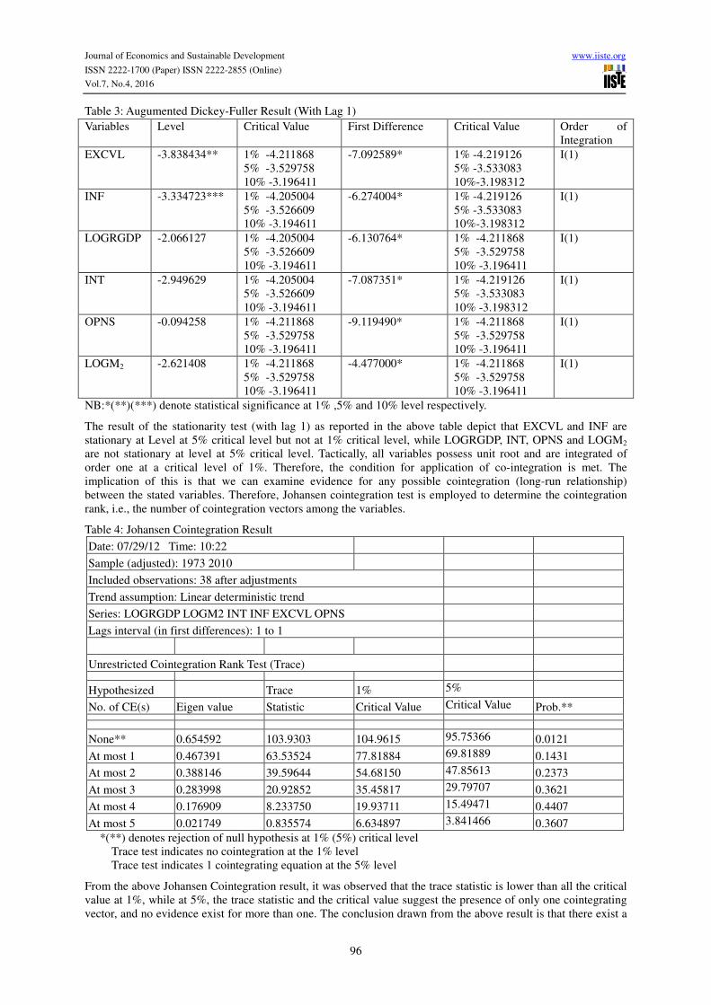
Table 3: Augumented Dickey-Fuller Result (With Lag 1)

NB:*(**)(***) denote statistical significance at 1% ,5% and 10% level respectively.

The result of the stationarity test (with lag 1) as reported in the above table depict that EXCVL and INF are

stationary at Level at 5% critical level but not at 1% critical level, while LOGRGDP, INT, OPNS and LOGM2

are not stationary at level at 5% critical level. Tactically, all variables possess unit root and are integrated of

order one at a critical level of 1%. Therefore, the condition for application of co-integration is met. The

implication of this is that we can examine evidence for any possible cointegration (long-run relationship)

between the stated variables. Therefore, Johansen cointegration test is employed to determine the cointegration

rank, i.e., the number of cointegration vectors among the variables.

Table 4: Johansen Cointegration Result

Date: 07/29/12 Time: 10:22



Trend assumption: Linear deterministic trend

Series: LOGRGDP LOGM2 INT INF EXCVL OPNS

Lags interval (in first differences): 1 to 1

Unrestricted Cointegration Rank Test (Trace)

Hypothesized Trace 1% 5%

No. of CE(s) Eigen value Statistic Critical Value Critical Value Prob.**

None** 0.654592 103.9303 104.9615 95.75366 0.0121

At most 1 0.467391 63.53524 77.81884 69.81889 0.1431

At most 2 0.388146 39.59644 54.68150 47.85613 0.2373

At most 3 0.283998 20.92852 35.45817 29.79707 0.3621

At most 4 0.176909 8.233750 19.93711 15.49471 0.4407

At most 5 0.021749 0.835574 6.634897 3.841466 0.3607

*(**) denotes rejection of null hypothesis at 1% (5%) critical level

Trace test indicates no cointegration at the 1% level

Trace test indicates 1 cointegrating equation at the 5% level

From the above Johansen Cointegration result, it was observed that the trace statistic is lower than all the critical

value at 1%, while at 5%, the trace statistic and the critical value suggest the presence of only one cointegrating

vector, and no evidence exist for more than one. The conclusion drawn from the above result is that there exist a

Variables Level Critical Value First Difference Critical Value Order of

Integration

EXCVL -3.838434** 1% -4.211868

5% -3.529758

10% -3.196411

-7.092589* 1% -4.219126

5% -3.533083

10%-3.198312

I(1)

INF -3.334723*** 1% -4.205004

5% -3.526609

10% -3.194611

-6.274004* 1% -4.219126

5% -3.533083

10%-3.198312

I(1)

LOGRGDP -2.066127 1% -4.205004

5% -3.526609

10% -3.194611

-6.130764* 1% -4.211868

5% -3.529758

10% -3.196411

I(1)

INT -2.949629 1% -4.205004

5% -3.526609

10% -3.194611

-7.087351* 1% -4.219126

5% -3.533083

10% -3.198312

I(1)

OPNS -0.094258 1% -4.211868

5% -3.529758

10% -3.196411

-9.119490* 1% -4.211868

5% -3.529758

10% -3.196411

I(1)

LOGM2 -2.621408 1% -4.211868

5% -3.529758

10% -3.196411

-4.477000* 1% -4.211868

5% -3.529758

10% -3.196411

I(1)



Vol.7, No.4, 2016

97

unique long-run relationship between economic growth (RGDP) and its determinants (LOGRGDP, LOGM2,

INT, INF, EXCVL and OPNS). In the short run, deviation from this relationship could occur due to shocks to any

of the variables. Thus, the error correction model (ECM) is applied to obtain the short-run dynamics.

5.2 Error Correction Model (Short-Run Analysis)

The short – run result of the model is hereunder presented:

Table 5: Short-Run Result of the Model

Dependent Variable: D(LOGRGDP)

Method: Least Squares

Date: 08/02/12 Time: 11:33



Variable Coefficient Std. Error t-Statistic Prob.

C 0.138313 0.056182 2.461857** 0.0194

D(LOGRGDP(-1)) 0.198839 0.150930 1.317427 0.1971

D(INF) 0.005806 0.003207 1.810738*** 0.0796

D(INF(-2)) 0.004918 0.003222 1.526254 0.1368

D(OPNS) -0.063369 0.028540 -2.220348** 0.0336

ECM(-1) -0.453165 0.126105 -3.593551* 0.0011







*(**) (***) indicates significant at 1, 5 and 10% level respectively.

The data for the ECM variable was obtained from the residual of the long-run equation; using the rate of change

on each of the variable and lagging them by 1 and 2 years respectively yield the over-parameterized equation

before elimination of highly insignificant variables with constant check on the Akaike and Schwarz criterion to

determine the stage at which the parsimonious equation was attained. The result shows that the estimated

specification for the LOGRGDP disequilibrium suggests that the speed of adjustment (the error-correction

mechanism) to long-run equilibrium is low. Specifically, over forty-five percent (45.32%) of the disequilibrium

errors, which occurred the previous year, are corrected in the current year.

The one lag value of LOGRGDP positively and insignificantly influenced the behaviour of D(LOGRGDP) in the

current period. In addition, change in current inflation rate D(INF) has a significant positive effect on

D(LOGRGDP), while two period lag inflation D(INF(-2)) exhibit a positive and insignificant effect on

D(LOGRGDP). Also, the current value of trade openness D(OPNS) exhibit a negative and statistically

significant influence on D(LOGRGDP).



Vol.7, No.4, 2016

98

5.3 Results of the Static Model

The long-run result of the model is hereunder presented:

Table 6: Long-run Result of the Model

Dependent Variable: LOGRGDP

Method: Least Squares

Date: 08/01/12 Time: 18:21



Variable Coefficient Std. Error t-Statistic Prob.

C 2.553955 0.716361 3.565181* 0.0011

LOGM2 0.831696 0.087652 9.488598* 0.0000

INT -0.028264 0.018105 -1.561097 0.1278

INF 0.000724 0.004902 0.147765 0.8834

EXCVL 0.005243 0.001992 2.631660* 0.0127

OPNS -0.135229 0.026800 -5.045901* 0.0000







*(**) (***) indicates significant at 1,5 and 10% level respectively.

The Coefficient of Determination value is high based on the above result indicating that about 91% variation in

Real GDP is explained by variations in the explanatory variables. The results also show that an increase in

money supply by 1% will increase RGDP by 83.17%. Growth of money supply shows a positive relationship and

this is in conformity with the a priori expectation of a positive relationship.

Interest rate is the cost incurred in the course of securing loans from banks. If interest rate increases by 1%,

RGDP will fall by 2.82% which is in line with the a-priori expectation that there exist a negative relation

between interest rate and economic growth (RGDP). When interest rate is low, more loans will be in demand by

economic agents which will lead to an increase in investment and output. Also, decrease in interest will lead to

low savings since the opportunity cost of parting with income will be low, economic agents (individuals, firms

and organizations) will prefer to hold their income in form of cash which brings about an increase in the level of

currency outside bank. In the same vein, inflation which is the persistent rice in price level exhibit positive trend

with output, as a 1% increase will lead to 0.07% increase in GDP which is not in conformity with the a-priori

expectation of a negative relationship between inflation and economic growth. This may be explained by the fact

that there is non-linearity in the effect of inflation on growth.

This result partly agrees with that of Grimes (1991) who found a positive relationship between inflation and the

economic growth for a short term, and a negative relationship between them for a long term.

Exchange Rate volatility shows the level of instability of the exchange rate, and a 1% increase of it will lead to

0.52% increase in RGDP which is not in line with the a-priori expectation of a negative relationship between

exchange rate volatility and economic growth; because, the more volatile the exchange rate, the riskier it is for

investors to invest, therefore leading to a negative effect on the economy. This finding is in conformity with that

of Azeez, Kolapo and Ajayi (2012), who concluded that exchange rate volatility has positive relationship with

the macroeconomic performance, and that the volatility affords investors to utilize the opportunity of an

appreciating Naira to import required capital technology.

In addition, trade openness shows the level of international movement of goods and services of a nation. 1%

increase in trade openness will lead to a fall in RGDP to the tune of 13.52%, which is not in conformity with the

a-priori expectation of a positive relationship between the variables concerned. The result here may not be so

worrisome as higher trade openness can create a countervailing effect of fuelling capital flight and corruption via



Vol.7, No.4, 2016

99

mis-invoicing. This is in line with the findings of Samra and Muhammad (2011) who investigated the causal link

between trade openness and economic growth for four (4) South Asian countries for the period 1972-1985; it was

observed that there exists negative relationship between GDP and openness.

6. Conclusion

Our results have shown clearly the beneficial effect of monetary aggregates in enhancing growth both in the

short run and in the long run. The lesson to be learnt here is that the Nigerian government and other developing

countries should strive to create conducive environment for sound macroeconomic policy necessary for smooth

flow of financial resources into productive sector of the economy.

Since trade openness significantly depresses growth, policies that ensure an increase in the domestic content and

the smooth running of Industrial and Manufacturing sector should be put in place. In order words, Nigerian

government should adopt strategic trade policies. It should examine the challenges, opportunities and constraints

they will face in participating in any trade liberalization (see also Ayadi, 2005).

Lastly, our result points to the possibility of a non-linear effect of inflation on growth. Meaning that there might

be a threshold of inflation rate consistent with growth, beyond which inflation can be distortionary. The nation’s

monetary authorities should therefore develop and implement measures that will ensure that both inflation and

foreign exchange rates are sustained at levels that will ensure increasing level of FDI inflows and output growth.

References

Adeyeye, E. A & Fakiyesi, T. O (1980), Productivity Prices and Incomes Board and Anti – Inflationary

Policy in Nigeria In The Nigerian Economy under the Military, Proceedings of the 1980 Annual

Conference of the Nigerian Economic Society, Ibadan, 257 – 273.

Agenor, P. (1991), A Monetary Model of the Parallel Market for Foreign Exchange. Journal of Economic

studies. Vol. 18 (4) 4-18.

Ajibefun, I. A. & Daramola, A. G. (2003), Efficiency of Microenterprises in Nigerian Economy. AERC

Research Paper 134, African Economic Research Consortium, Nairobi.

Akinnifesi E.O. (1977): Credit Ceilings, Absorptive Capacity and Inflation in Nigeria (1962–1980).

Central Bank of Nigeria, Research Department, Lagos, Unpublished Discussion Paper.

Ayadi, F. S. (2005), A Vector Autoregressive Analysis of Trade-Environment Linkage in Nigeria. World

Review of Science, Technology and Sustainable Development. 2 (2) 191-201.

Azeez, B. A., Kolapo, F. T. & Ajayi, L. B.(2012), Effect of Exchange Rate Volatility on Macroeconomic

Perfoprmance in Nigeria. Interdisciplinary Journal of Contemporary Research in Business. 4 (1) May

2012.

Barbone, L. & Rivera-Batiz, F. (1987), Foreign Capital and Contractionary Impact of Currency

Devaluation, With Application to Jamaica. Journal of Development Economics. 26, 1-15.

Barro, R. J. (1996), Determinants of Economic Growth: A Cross-Country Empirical Study. NBER

Working Papers 5698, National Bureau of Economic Research, Inc.

Bruno, M. (1979), Stabilization and Stagflation in a Semi- Industrialized Economy. In Dornsbusch, R.

and Frankel, J. (Ed.s): International Economy policy. John Hopkins University Press, Baltimore, MD.

Bruno, M. & Easterly, W. (1996), Inflation and Growth: In Search of Stable Relationship. Federal

Reserve Bank of St. Louis Review. 78 (3).

Cooper, R.N. (1971), Currency Devaluation in Developing Countries. Essay in International Finance.

No. 86, International Finance Section, Princeton University.

Dordunoo, C. K. & Njinkeu, D. (1997), Foreign Exchange Rate Regimes and Macroeconomic

Performance in Sub-Saharan Africa. Journal of African Economies. 121-149.

Du, H. & Zhu, Z. (2001). The Effect of Exchange-Rate Risk on Exports: Some Additional Empirical

Evidence. Journal of Economic Studies. 28(2), 106 -123.

Engle, R.F. and Granger, C.W.J. (1987), “Cointegration and Error Correction: Representation, Estimation

and Testing,” Econometrica. Vol. 55, pp 251-276.

Ghosh, A. R., Gulde, A., Ostry, J.D., & Wolf, H.C. (1997), Does the Nominal Exchange Rate Regime



Vol.7, No.4, 2016

100

Matter? NBER Working Paper no. 5874.

Grimes, A. (1991), The Effects of Inflation on Growth: Some International Evidence. Weltwirtschaftliches

Archive. 127, 631-644.

Harms, P. & Kreschmann, M. (2009), Words, Deeds and Outcomes: A Survey on the Growth Effects of

Exchange Rate Regimes. Journal of Economic Surveys. 23(1), 139-164.

Hasanov, F. (2011), Relationship Between Inflation and Economic Growth in Azerbaijani Economy: Is

There Any Threshold Effect? MPRA Paper 33494, University Library of Munich, Germany.

Hashim, I. A & Zarma, A. B. (1996), The Impact of Parallel Market on the Stability of Exchange Rate:

Evidence from Nigeria. NDIC Quarterly. 7(2).

Hirschman, A.O. (1949), Devaluation and the Trade Balance. A Note Review of Economics and Statistics.

31, 50 -53.

Honohan, P. & Lane, P. R. (2003), Divergent Inflation Rates in EMU. Economic Policy. 37, 359-94.

Hyder, Z. & Shah, S. (2004). Exchange Rate Pass-Through to Domestic Price in Pakistan. Working

Paper, .5, State Bank of Pakistan.

Ikhide, S. I. and Yinusa, D. O. (1998). The Impact of Financial Liberalisation on the Finance of Small and

Medium Scale Enterprises in Nigeria. Research Report 12. Development Policy Centre, Ibadan.

Iyoha, A. M. & Oriakhi, D. (2002), Explaining African Economic Growth Performance: the Case of

Nigeria. Report on Nigerian Case Study Prepared for AERC Project on, Explaining African Economic

Growth Performance.

Krugman, P. R. & Taylor, L (1978), Contractionary Effect of Devaluation. Journal of International

Economics. 8 Nov 3, 183-227.

Mishkin, F. S. & Posen, A. S. (1997), Inflation Targeting: Lessons from Four Countries. NBER Working

Paper 6126, August 1997.

Nwankwo, G. O. (1982), Inflation in Nigeria- Causes and Cure. In Onitiri, H.M.A. and Awosika, K.

(Ed.s) Inflation in Nigeria. NISER, Ibadan.

Obstfeld, M. & Rogoff, K. (1995), Exchange Rate Dynamics Redux. Journal of Political Economy. . 103,

624-659.

Odusola & Akinlo, E. A. (2001), Output, Inflation, and Exchange Rate in Developing Countries: An

Application to Nigeria. The Development Economies. 34(2), 199-222.

Ogunleye, E. K. (2008), Natural Resource Abundance in Nigeria: from Dependence to Development.

Resources policy.

Ogunleye, E. K. (2010), Exchange Rate Volatility and Foreign Direct Investment in Sub-Saharan Africa:

Evidences from Nigeria and South Africa. Retrieved from www.resourcespolicy on7/2/2010.

Ohiria, O., Saliu, T. S. & Schuller, B. (2008), Exchange Rate Variation and Inflation in Nigeria.

University of Skovde.

Onitiri, H. M. A. & Awosika, K. (1982), Inflation in Nigeria. Proceedings of a National Conference

Convened by the Nigerian Institute of Social and Economic Research, Ibadan.

Osakwe, J. O.(1983), Government Expenditure, Money Supply and Prices, 1970–1980. CBN Economic

and Financial Review. 21(2), June.

Petreski, M. (2009), Exchange-Rate Regime and Economic Growth: A Review of the Theoretical and

Empirical Literature. Economic Open – Assessment E-Journal. Discussion Paper 2009-31/July 8, 2009

Retrieved on 02/11/12 at http://www.economics-ejournal.org/economics/discussionpapers/2009-31

Phylaktis, K. & Girardin, E. (2001), Foreign Exchange Markets in Transition Economics, China. Journal

of Development Economics. 64, 215-35.

Rosenberg, M. R. (2003), Exchange Rate Determination. Models and Strategies for Exchange Rate

Forecasting. McGraw-Hill.

Samra, B. and Muhammad, W. S. (2011), Trade Openness and its Effects on Economic Growth in



Vol.7, No.4, 2016

101

Selected South Asian Countries: A Panel Data Study. International Journal of Human and Social

Sciences.. 6(2).

Sanusi, J. O. (2004), Exchange Rate Mechanism: The Current Nigerian Experience. Being a Paper

Delivered at the Laundries of the Nigerian – British Chamber of Commerce, Feb. 24, 2004.

Stotsky, G. .J., Ghazanchyan, M., Adedeji, A. & Maehle, N. (2012), The Relationship Between the

Foreign Exchange Regime and Macroeconomic Performance in Eastern Africa. IMF Working Paper

WP/12/148. June 2012.

Wijnbergen, S. (1989), Capital Control and the Real Exchange Rate. NBER Working Paper 2940, April

1989.

Dr. AYADI, Folorunso Sunday is a Senior lecturer and a Ph.D. holder in Economics (majoring in

Environmental and Resource Economics) at the University of Lagos, Nigeria. He has taught Economics at the

undergraduate as well as postgraduate levels for several years. Some of his postgraduate classes include

Microeconomics of Environment and Macroeconomics of Environment and policy. He also has consultancy

experience in management and tax auditing with a tax consultancy firm in Lagos for some years. He has received

some scholarly awards as best paper presenter and best track presenter in international conferences. He has

publications in various academic journals (including the World Review of Science, Technology and Sustainable

Development, Oxford Journal etc.), chapters in books and conference proceedings. His current research and

consultancy interests are in the area of Economics of pollution control and wastes management, natural

resources Economics and Management, Urban Management, Poverty, Development Economics, Globalization

and; Energy in Developing Economies.

Olajide Anuoluwa JEREMIAH earned his Bachelor's degree in Economics from one of the Nigerian's top

Universities (University of Lagos, Nigeria). He is currently studying for his Master’s in the same department.

Olajide Anuoluwa Jeremiah has Strong and insatiable quest for analytical research and he is coined as a lecturer

in the making. His undergraduate research work was seen as outstanding, and thus regarded as one of the best

undergraduate research work of his time by lecturers and the undergraduate project defense panelists. His areas

of interest include Microeconomic research, Macroeconomics and development economics among others.

Date post:	22-Dec-2021
Category:	Documents
Upload:	others
View:	3 times
Download:	0 times

Price Instability, Exchange Rate Volatility and the ...

Documents