Swedish University of Agricultural Sciences Faculty of Natural Resources and Agricultural Sciences Department of Economics Price transmission system in Ethiopian coffee Market Mengistu E. Seyoum Master’s thesis · 30 hec · Advanced level Environmental Economics and Management - Master’s Program Degree thesis No 625 · ISSN 1401-4084 Uppsala 2010 brought to you by CORE View metadata, citation and similar papers at core.ac.uk provided by Epsilon Archive for Student Projects
Transcript
Swedish University of Agricultural Sciences Faculty of Natural Resources and Agricultural Sciences Department of Economics
Price transmission system in Ethiopian coffee Market
Mengistu E. Seyoum
Master’s thesis · 30 hec · Advanced level Environmental Economics and Management - Master’s Program Degree thesis No 625 · ISSN 1401-4084 Uppsala 2010
brought to you by COREView metadata, citation and similar papers at core.ac.uk
Price transmission system in Ethiopian coffee market Mengistu E. Seyoum Supervisor: Hans Andersson, Swedish University of Agricultural Sciences Department of Economics Examiner: Carl-Johan Lagerkvist, Swedish University of Agricultural Sciences Department of Economics Credits: 30 hec Level: Advanced E Course title: Degree Project in Business Administration Course code: EX0536 Program/Education: Environmental Economics and Management - Master’s Program Place of publication: Uppsala Year of publication: 2010 Cover picture: visionmagazine.com Name of Series: Degree project No: 625 ISSN 1401-4084 Online publication: http://stud.epsilon.slu.se Key words: price transmission, asymmetry, market integration, coffee, Ethiopia.
Swedish University of Agricultural Sciences Faculty of Natural Resources and Agricultural Sciences Department of Economics
iii
Acknowledgments
This paper has dedicated to the Ethiopian coffee farmers who are seeking to get the right share price and still some of do the daily chores their ancestors have done years before.
Moreover, I would like to thank and express my sincerest regards to
Ø My supervisor professor Hans Andersson for his continuous support. He is patiently enough to listen and give me advice. I always remember his guidance, encouragement, academic stimulus, and generous help. He taught me not only the knowledge how to write thesis, but also infused with enthusiasm how to find and cope with different opportunities in my future life, which always be a challenge.
Ø Dr Taddesse Kuma from Ethiopian developmental research institute for compiling and sending me the data as getting data is costly especially for students.
Ø Thanks for George Abdu and Lennart Norell for sharing me their ideas in mathematical part of the thesis.
Ø For all Swedish University of Agricultural Science department of economics staffs, especial thanks for Bo Öhlmér, Cecilia Mark-Herbert and Kristina Jansson in any kind of their help.
Ø Lastly but not defiantly the list, I express my gratitude to my family, my girl friend, relatives and friends who are very far from me but sending me their valuable wards.
iv
ABSTRACT
Price is the most vital element in market interaction. If there is an international free trade
and the domestic market of one country is interconnected with the international market,
and if there is a price shocks in one market, the impact will have the same in the other
market. This is the major concept of price theory and the concept of price transmission
explored here.
This paper analyses the price transmission system on the level of the producer, the auction
market and the foreign (international) market in the Ethiopian coffee market in the short as
well as in the long run. The study cover the periods from December 1991 to April 2009,
based on 209 observations. Using the vector error correlation method and by using EVIEWS
and STATA software, the study attempts to examine the three most important elements in
price transmission analysis. These are causality, speed of adjustment and asymmetric
response.
The finding of this study shows that, there is a long run cointegration between these three
markets. The long run analysis further shows that if there is a 10% change auction market,
the long run impact on the producer price is 9.56%, implies these two markets moves closely
together in the long run. On the other hand, a 10% change in foreign price has only 6.5% and
5.7% impact on the auction and producer market respectively in the long run.
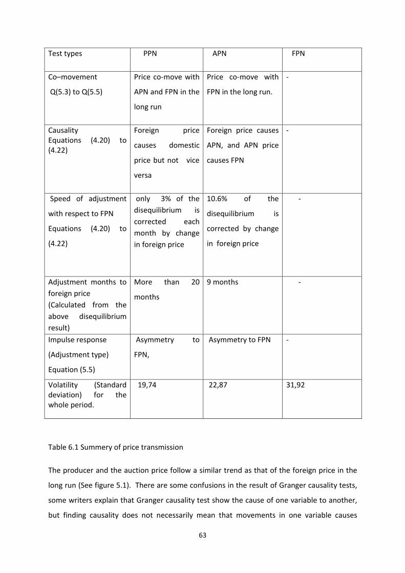
The result from the VEC model suggested that the adjustment coefficient for producer price
is only 3% if there is a shock in the foreign coffee market by one unit in the short run. This
means that only 3% of the shock is transmitted to the domestic market in each month. 3%
adjustment coefficient is quite small and insignificant. This indicates that lagged producer
price is insignificant in the foreign market. The result on the VECM indicates that the
producer market and the foreign market are poorly dependent and have very weak
relationships to one another as comparing to auction to the foreign market. Because of this,
the transmission period from producer market to foreign market takes more than 12
months.
v
This is a clear indication for the lack of market infrastructure, information asymmetry and
poor transportation system. A more organized market infrastructure may improve the
supply channel and thereby raise the farmer’s income.
vi
ABBREVIATIONS
PPN = average cash received by coffee producer in Ethiopia. The price is calculated as, local
currency multiplied by appropriate exchange rate to get monthly average producer price in
US cents per Pound. US cent per pound is the measurement of coffee price at the
international level.
APN = the national average auction price of coffee in Ethiopia.
FPN = the national average foreign price of coffee in Ethiopia. It is calculated as the auction
price plus transportation to the port plus carrying cost to the ship.
ICO= international coffee organization
APT = asymmetric price transmission
VECM = vector error correction model
VAR- ECM = vector autoregressive error correlation model
1.1 GENERAL BACKGROUND ABOUT COFFEE AND ETHIOPIA ....................................................................................... 2
1.2 PROBLEM FORMULATION .............................................................................................................................. 4
1.4 THE SIGNIFICANCE OF THE STUDY ................................................................................................................... 7
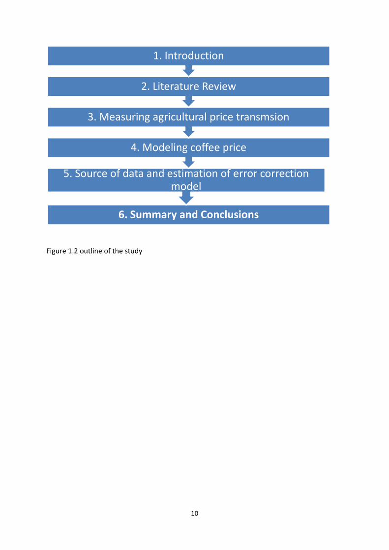
1.7 STRUCTURE OF THE RESEARCH ....................................................................................................................... 9
2 LITERATURE REVIEW ........................................................................................................................ 11
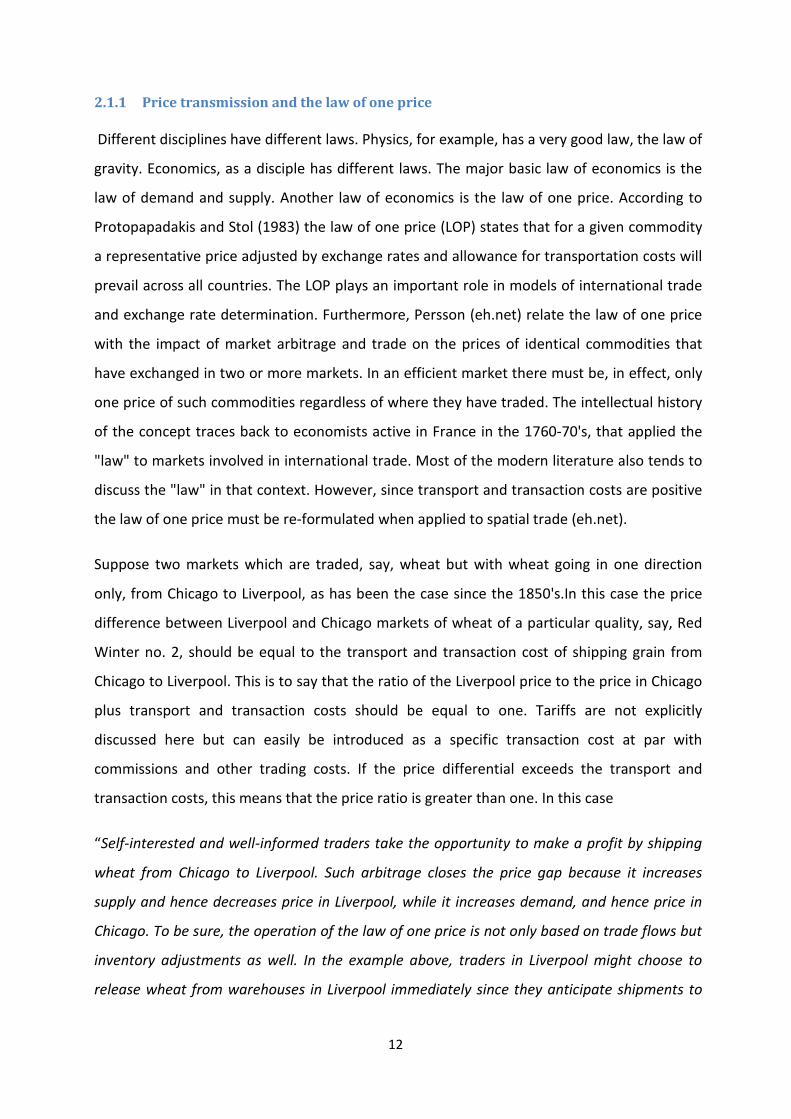
2.1 PRICE TRANSMISSION AND MARKET INTEGRATION ............................................................................................ 11
2.1.1 Price transmission and the law of one price .................................................................................... 12 2.1.2 Key determinants of price transmission ........................................................................................... 15
2.2 PRICE ASYMMETRY AND MARKET INTEGRATION ............................................................................................... 15
2.2.1 Types of asymmetry ......................................................................................................................... 18 2.2.1.1 Asymmetry with reference to speed and magnitude ............................................................................. 19 2.2.1.2 Negative Vs. positive APT ........................................................................................................................ 20 2.2.1.3 Vertical Vs. spatial APT ............................................................................................................................ 21
2.3 FACTORS THAT AFFECTS AGRICULTURAL COMMODITY PRICES ..................................................................................... 30
3 METHODS FOR MEASURING AGRICULTURAL PRICE TRANSMISSION .......................... 32
3.1 HOW DO WE MEASURE PRICE TRANSMISSION? ................................................................................................ 32
3.1.1 Ratio of percentage changes between two time periods ................................................................ 32 3.1.2 Correlation analysis ......................................................................................................................... 33 3.1.3 Regression analysis .......................................................................................................................... 34 3.1.4 Co-integration analysis .................................................................................................................... 37
4 MATHEMATICAL FORMULATION OF COFFEE PRICE IN ETHIOPIA ................................ 36
5 SOURCE OF DATA AND ESTIMATION OF ERROR CORRELATION MODEL ................... 42
5.1 SOURCE OF DATA ...................................................................................................................................... 42
5.2 COFFEE PRICE AFTER 1991 IN ETHIOPIA ........................................................................................................ 43
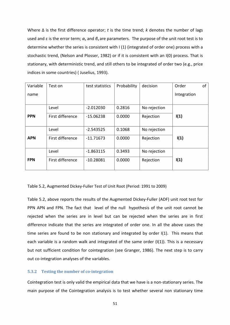
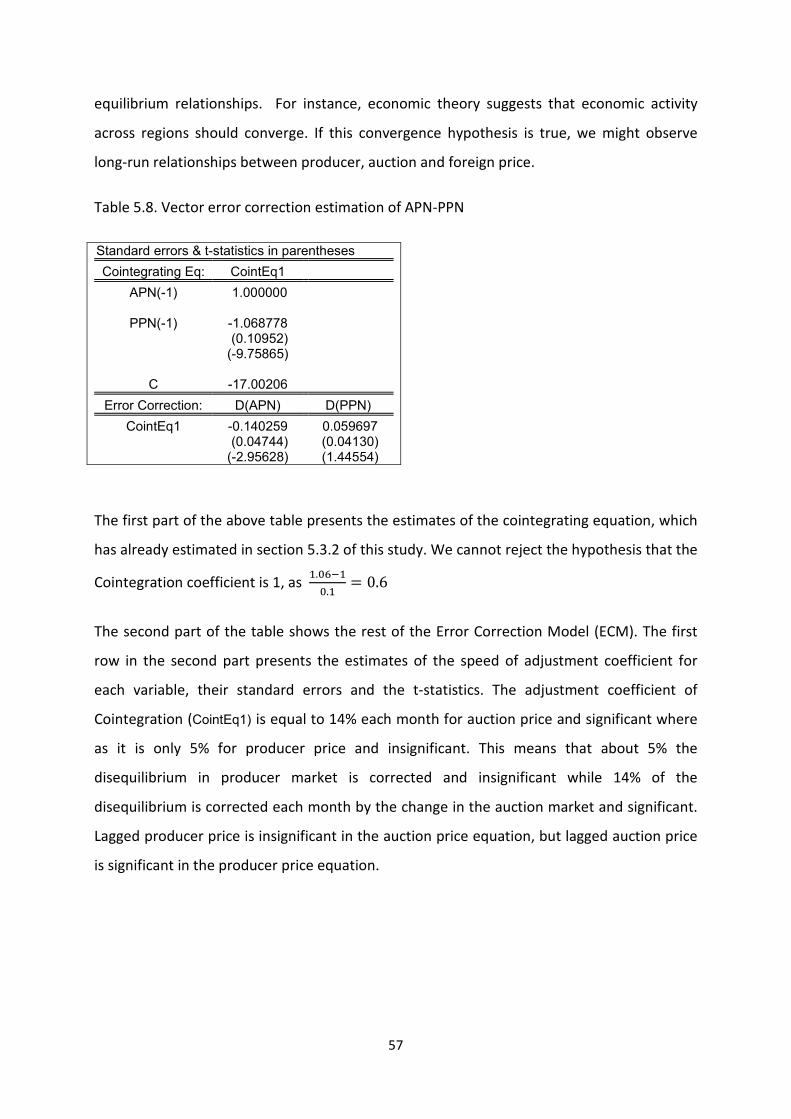
5.3 INTERPRETATION OF THE MODELS ................................................................................................................. 50
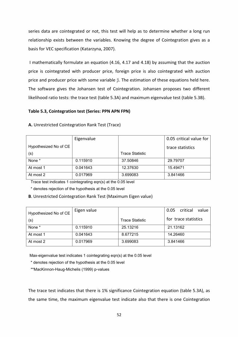
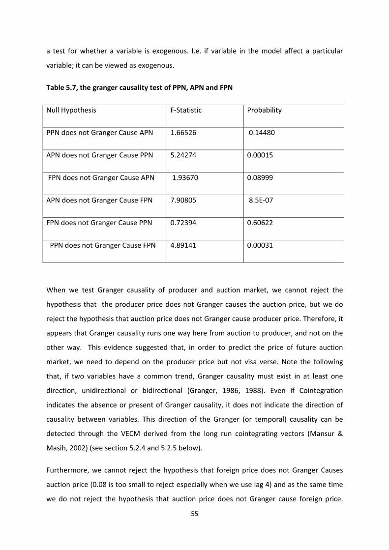
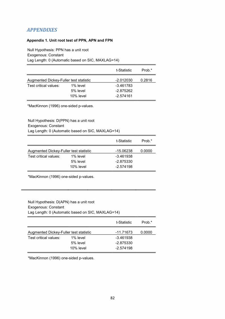
5.3.1 Augmented Dickey Fuller (ADF) unit root test ................................................................................. 50 5.3.2 Testing the number of co-integration .............................................................................................. 51 5.3.3 The Granger Causality test .............................................................................................................. 54 5.3.4 Estimation of vector error correction model (VEC) .......................................................................... 56
REFERENCE LIST ........................................................................................................................................... 68
LITERATURE AND PUBLICATIONS ................................................................................................................................ 68
INTERNET SOURCES ................................................................................................................................................. 78
SOFTWARE USED .................................................................................................................................................... 81
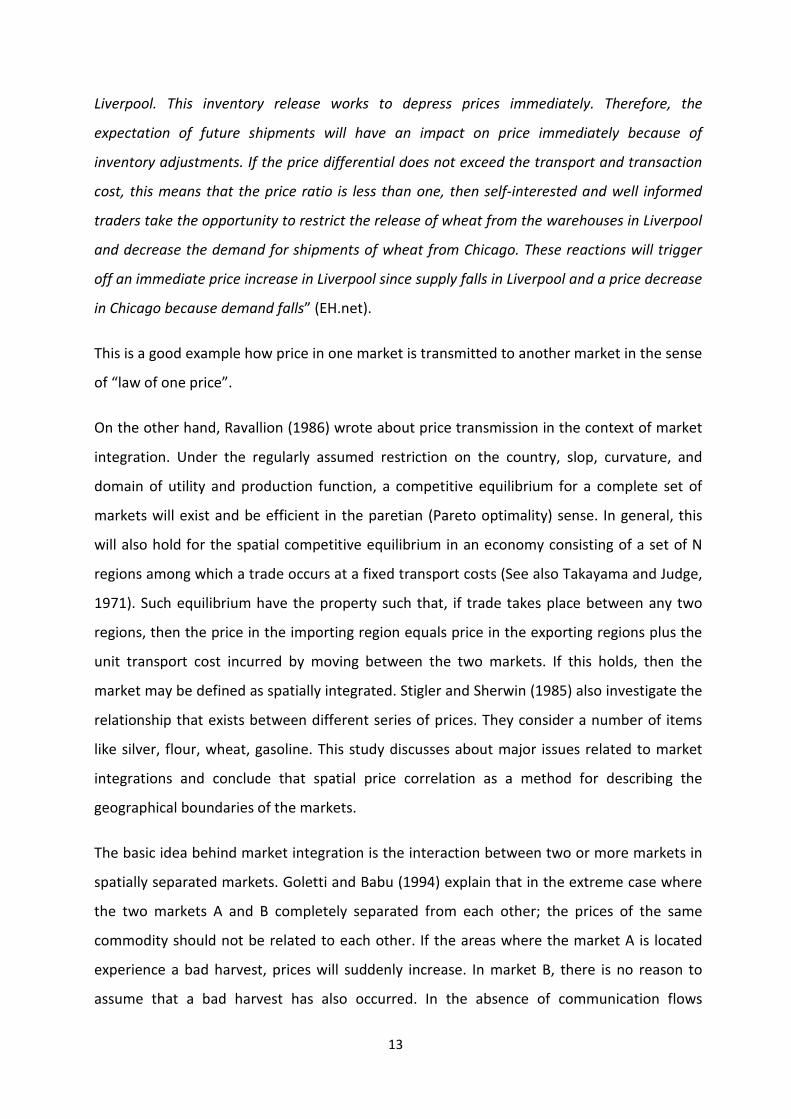
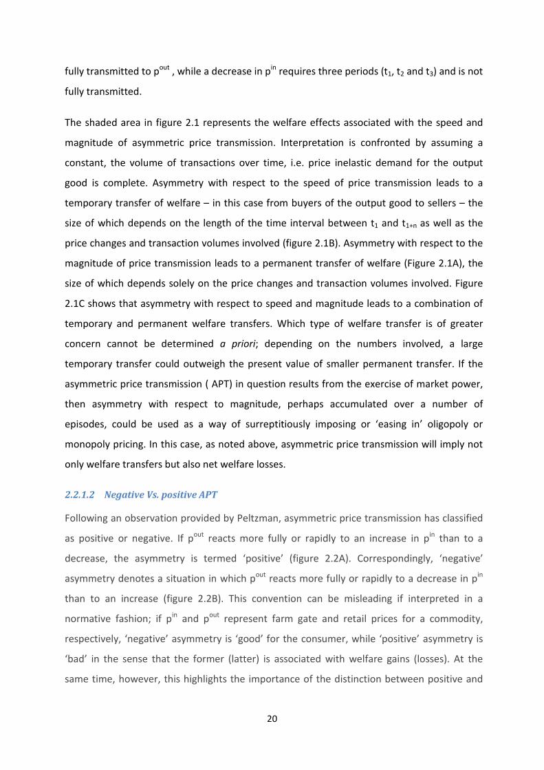
Figure 2.2, positive and negative asymmetric price tran
2.2.1.3 Vertical Vs. spatial APT
This classifies whether asymmetric price transmissi
transmission system. A very good example of vertical AP
“Farmers and consumers often complain that increase
rapidly transmitted to the wholesale and retail levels
prices. An example of spatial APT would be a rise in the
more pronounced reaction in the Canadian export price
same magnitude. Spatial APT, like vertical APT, can b
Positive APT be defined as a set of reactions according to which any price movement that squeezes the margin (i.e. an increase in pin or a fall in pout ) is transmitted more rapidly and/or completely (to pout or pin , respectively) than the equivalent movement that stretches the margin.
smission
on affects vertical or spatial price
T, given by Von Cramon and Meyer is
s in farm prices are more fully and
than equivalent decreases in farm
US export price for wheat causing a
than a corresponding reduction of the
e classified according to speed and
APT is negative when price movements that stretch the margin are transmitted more rapidly and/or completely than movements that compress it.
22
magnitude, and according to whether it is positive or negative” (Meyer and Cramon-
Taubadel, 2004, pp 5)
2.2.2 Causes of asymmetry price transmission
There are a numbers of factors that believed to be the cause of price asymmetric according
to different literatures but for this particular analysis it is better to divide in to three parts by
considering the first two big factors and categorizing another factors as miscellaneous.
2.2.2.1 Adjustment costs
According to economics dictionary, adjustment cost is the cost to a firm of altering its level of
output. For example, it may be desirable for a firm to cut down on its output, but doing this
will create adjustment costs such as redundancy payments and lower staff morale. On
reflection of its adjustment costs, it may be more desirable to keep producing at a suboptimal
level. Similarly, a rapid expansion in output may create problems such as difficulties in
negotiating a bigger plant to rent and the difficulties in hiring more workers
(economicshelp.org).
Firms may face different adjustment costs depending on whether prices are rising or falling
(Bailey and Brorsen, 1989). Competition between meat packers faced with high fixed costs
and excess capacity, for example, might result in farm prices that are bid up rapidly in
response to increased demand for meat products, but fall more slowly as demand weakens.
In the short run, margins may thus be reduced in an attempt to keep a plant operating at or
near capacity. Therefore, because of competition between different packers, farm prices may
be bid up more quickly than they are bid down (negative APT).
Similarly, Ball and Mankiw (1994) posit a model in which firms face menu costs (the costs
involved in changing nominal prices, such as the cost of reprinting catalogues, etc.) and
inflation. In this environment, shocks that increase a firm's desired price will trigger larger
responses than shocks that reduce it, because firms will take advantage of positive shocks to
correct also for accumulated and anticipated inflation, while inflation will already have
affected some of the adjustment made necessary by negative shocks. This asymmetry,
however, disappears under price stability. Moreover, during periods of sustained deflation,
the asymmetry is reversed: relative prices are adjusted downward more quickly than they are
23
adjusted upward. Thus, the model may prove useful for understanding differences in price
adjustment under different monetary regime. Contrary to this, Peltzman (2000) indicates
that asymmetric adjustment is prevalent with retail prices rising faster, as compared to
falling, while this asymmetry is not related to inventory costs, menu costs and imperfect
competition. Such findings not only suggest that asymmetry is the rule rather than the
exception in market price adjustment but raise a number of questions related to the
suitability of empirical price-based tests and the conventional theory of prices.
Ward (1982) suggests that retailers may be hesitant to raise prices of perishable goods for
fear that they could end up holding spoiled stocks. Wholesale prices are shown to lead both
retail and shipping point prices. Asymmetry in the retail-wholesale response indicates that
wholesale price decreases are reflected at the retail more so than are wholesale price
increases. Wholesale price decreases are more fully passed through to the shipping point
relative to wholesale increases. In all these cases, the speed of price transmission is
asymmetric, but there is no reason to expect that long-run elasticity of price transmission will
be asymmetric as well. Heien (1980) on the other hand argue that increases in wholesale
prices are transmitted to the retail level via mark-up-type pricing behavior. This behavior is
shown to be consistent with firm optimization under the assumption of constant returns to
scale and Leontief production technology at the retail level. He concludes that changing
price is not a problem for perishables, but for items with a long shelf life, price changes are
costly both in terms of time to put on new labels and in goodwill lost.
2.2.2.2 Market power
Market power is defined as the ability of the firm to raise prices above its marginal cost.
Lands and Posner (1981) further define market power as the ability of the firm (or a group of
firms, acting jointly) to raise price above the competitive level without losing many sales so
rapidly that the price increases are rendered, unprofitable and must be rescinded. Along
production chains, some agents may behave as price makers while some other as price
takers, depending on the degree of concentration of each industry. It may be the case that,
for example input price increased in an industry may be passed over to consumers, while
input price decreases can be captured in the markup of the industry (Wohlgenant, 1999;
Azzam, 1999; Goodwin and Holt, 1999).
24
Different articles on asymmetric price transmission explain that non-competitive market as a
source of APT. Meyer and Taubadel (2004) explain that this is more common in agricultural
commodities. Farmers at the begging of the marketing chain and consumer at the end of the
marketing chain frequently imagine that imperfect computation in processing and selling
allows intermediaries to use market power. This could be resulted from a positive
asymmetric price transmission. Therefore, it has expected that margin-squeezing increases in
input prices (or decreases in output prices) will be transmitted faster and/or more completely
than the corresponding margin-stretching price changes. On the other hand, McCorriston and
Rayner (1998) show how a price change in the farm level is transmitted to the retailer sector.
A price transmission elasticity is derived which is shown to depend on the degree of market
power in the food industry and the nature of the food industry’s processing technology. They
further develop a model to show the impact of market power on the intermediate stage on
price transmission on the food sector can lead to imperfect price transmission without
considering asymmetry. In their findings the offsetting role of processing technology and
market power in determining the extent of price transmission is highlighted.
Von Cramon et al. (1997) argue that marketing chains for food products are often much less
concentrated at the farm level than at higher levels. He explains that
“Oligopolistic processors, for example, might react collusively more quickly to shocks that
squeeze their margins than to shocks that stretch it, resulting in asymmetric short-run
transmission. In an attempt to hide the exercise of market power behind the 'confusion'
created by major shocks, processors could also react less completely to shocks that stretch
their margins, leading to asymmetric long-run transmission “ (Van Cramon 1997, pp 10).
R. Ward and Kinnucan and Forker (1987) suggest market power might explain the findings of
asymmetric price adjustments. Scherer (1980) argues price inflexibility may exist in industries
characterized by non price competition, high market concentration ratios, and large
advertising expenditures. This idea was further supported by Bailey and Brorsen (1989:247)
by considering some examples. According to them asymmetry could result if firms perceive
kinked demand curve. The kink in the demand curve can result when individual firms believe
that no competitor will match a price increase, whereas all firms would match a price cut.
The opposite is also possible when the individual firm believes that all its competitors would
25
match a price increase. Here there is no clear a priori how price transmission will be skewed.
Furthermore, concentration is perhaps a necessary but certainly not a sufficient condition for
the exercise of market power and the theoretical and empirical evidence on the relationship
between these two phenomena is inconclusive (Van Cramon 1997, Weaver, 1989; Goodwin,
1994).
Luoma (2004) studied the transmission of producer price changes to consumer prices in
Finnish beef and pork markets. According to the previous studies price transmission has
asymmetric because of market power and adjustment costs. Here they argued that market
power is the most likely explanation for asymmetric price transmission in the long run. In
imperfectly competitive markets, retailers may keep price levels relatively fixed for long
periods, or oligopolies may react quicker to declining margins by utilizing their market power.
The reason they do this is to maintain market shares, keeping long-run rather than short-run
profits in mind. Hence, market power can affect price transmission in opposite ways.
Several economists have been studying price asymmetry in the oil industry and the causes of
it. Borenstein (1997) study vertical price transmission from crude oil to gasoline prices, and
conclude that:
“Downward stickiness of retail prices for gasoline in an oligopolistic environment will lead to
positive asymmetry. They assume that in the presence of imperfect information about the
prices charged by other firms, the old output price offers a natural focal point following
changes in the input price. While increases in the price of crude oil will lead to an immediate
increase in gasoline prices, because margins are squeezed, cost decreases won’t lead to
immediate output price decreases because firms will maintain prices above the competitive
level as long as their sales remain above a threshold level” (Borenstein et al. 1997 pp. 324).
He further argues that “lags in the adjustment of price to input cost changes are not
consistent with simple models of either competitive markets or monopoly” (pp 301). The price
set by a profit maximizing monopolist depends on marginal costs. The profit maximizing
monopolist thus wants to change his price every time marginal costs change. Therefore, in
the case of transparency and perfect flexibility, there is no ground for either upstream or
downstream time lags. By the same token, Balke, Brown and Yucel (1998) explain that in the
retail gasoline market, consumer search costs could lead to temporary market power for gas
26
stations and an asymmetric response to changes in the wholesale price of gasoline (See BCG,
Norman and Shin 1991, Borenstein 1991, and Deltas 1997). Each gas station has a locational
monopoly that is limited only by consumer search. After consumers have searched, the profit
margins at each gas station are pushed down to a roughly competitive level. When wholesale
prices rise, each station acts to maintain its profit margins and quickly passes the increase on
to customers. When wholesale prices fall, however, each station temporarily boosts its profit
margins by slowly passing the decrease on to customers. Only after the customers engage in
a costly and time-consuming search to find the lowest prices are the stations forced to lower
prices to a competitive level.
Many paper's emphasis the idea that market power that consider APT caused not by input
price change, but by shifting the output demand. In a paper on imperfect information in a
competitive duopoly, Damania & Yang (1998) stress the main causes of asymmetric price
transmission is potential punishment. This model stress that the demand of the product is
expected to fluctuate between high and low states randomly. Punishment occurs if a firm
believes that its competitor is undermining a collusive price. Given the possibility of
punishment, firms facing low demand dislike a price reduction, while prices can be increased
without fear of punishment following a switch to the high demand situation. Kovenock and
Widdows (1998) also present a simple price leadership model in which equilibrium behaviour
exhibits price rigidity following downward demand shocks and price flexibility after an
increase in demand. The source of this asymmetric rigidity lies in the fact that leader-follower
equilibrium prices are lower than their collusive levels and that any firm leading a round of
price adjustment must anticipate the optimal price response of the follower. In addition, they
found that there is a range of shocks, both positive and negative, in which the identity of the
price leader is endogenous.
To sum up, many authors agree that market power leads to asymmetric price transmission.
Most writers on these issues believe that the cause of positive APT is market power. Meyer
and Cramon-Taubadel (2004) explain that the situation is differing in the case of pure
monopoly and common oligopoly context. In a pure monopoly context, this would appear to
be reasonable. However, in the more common oligopoly context, both positive and negative
APT is conceivable, depending on market structure and conduct.
27
2.2.2.3 Miscellaneous causes
There are other miscellaneous causes, in addition to transfer costs and market power that
causes price asymmetry. In spatial markets, for example, asymmetries may result from
inventory holding behavior in domestic markets as stock accumulation may result from high
international price expectation (Maccini, 1978; Blinder, 1982). Different reaction to increase
and decrease of input costs is the other reason for asymmetric price adjustment, as
competition between wholesalers with high fixed costs and excess capacity may result in
producer prices that increase rapidly when demand for processed product is high, but
decrease at a slower rate when demand is low (Bailey and Brorsen, 1989; Kovenock and
Widows, 1998). Besides these Search costs associated with asymmetric information may lead
to asymmetric price adjustment (Bénabou and Gertner, 1993).
28
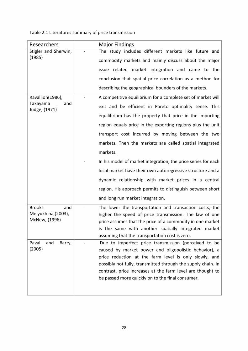
Table 2.1 Literatures summary of price transmission
Researchers Major Findings Stigler and Sherwin, (1985)
- The study includes different markets like future and
commodity markets and mainly discuss about the major
issue related market integration and came to the
conclusion that spatial price correlation as a method for
describing the geographical bounders of the markets.
Ravallion(1986), Takayama and Judge, (1971) - A competitive equilibrium for a complete set of market will
exit and be efficient in Pareto optimality sense. This
equilibrium has the property that price in the importing
region equals price in the exporting regions plus the unit
transport cost incurred by moving between the two
markets. Then the markets are called spatial integrated
markets.
- In his model of market integration, the price series for each
local market have their own autoregressive structure and a
dynamic relationship with market prices in a central
region. His approach permits to distinguish between short
and long run market integration.
Brooks and Melyukhina,(2003), McNew, (1996) - The lower the transportation and transaction costs, the
higher the speed of price transmission. The law of one price assumes that the price of a commodity in one market is the same with another spatially integrated market assuming that the transportation cost is zero.
Paval and Barry, (2005) - Due to imperfect price transmission (perceived to be
caused by market power and oligopolistic behavior), a price reduction at the farm level is only slowly, and possibly not fully, transmitted through the supply chain. In contrast, price increases at the farm level are thought to be passed more quickly on to the final consumer.
29
Table 2.2 Literatures summary on price asymmetry
Researchers Major findings Von Cramon-Taubadel (1998)
- He analyzed German pork market with an earlier non-symmetric error correction model and found evidence of asymmetric price transmission in the form that wholesale prices react more strongly to compress than stretched margins
Wang, Tadesse and Rayner (2006) Luoma (2004)
- explored the impact of market power on the degree of price transmission allowing for the interaction between oligopoly power in the food retail sector and oligopsony power in the farm sector when industry technology is characterized by non-constant returns to scale
- Market power is the most likely explanation for asymmetric price transmission in the long run. In imperfectly competitive markets, retailers may keep price levels relatively fixed for long periods, or oligopolies may react quicker to declining margins by utilizing their market power.
Meyer and Taubadel (2004)
- Farmers at the beginning and consumers at the end of the marketing chain often suspect that imperfect competition in processing and retailing allows intermediaries to use market power.
Ward (1982)
- Examined price transmission for a number fresh produce items is U.S. market and found that price rises were not passed on to the same extent as were price falls, he mentioned many reason including the perishability of produce, which implied that retailers would be unlikely to raise prices and risk stock moving more slowly and deteriorating
Maccini, 1978; Blinder, 1982 Brorsen, 1989; Kovenock and Widows, 1998
- In spatial markets, asymmetries may result from inventory holding behavior in domestic markets as stock accumulation may result from high international price expectation.
- Different reaction to increase and decrease of input costs is the other reason for asymmetric price adjustment
(Bénabou and Gertner, 1993
- Search costs associated with asymmetric information may lead to asymmetric price adjustment
30
2.3 Factors that affects agricultural commodity prices
The general price level of an agricultural commodity, whether at a major terminal, port, or
commodity futures exchange, is influenced by a variety of market forces that can alter the
current or expected balance between supply and demand. Accoording to Randy (2006) many
of these forces emanate from domestic food, feed, and industrial-use markets and include
consumer preferences and the changing needs of end users; factors affecting the production
processes (e.g., weather, input costs, pests, diseases, etc.); relative prices of crops that can
substitute in either production or consumption; government policies; and factors affecting
storage and transportation. International market conditions are also important depending on
the “openness” of a country’s domestic market to international competition, and the degree
to which a country engages in international trade.
Besides these factors in analyzing the coffee prices, we have to keep in mind factors that
could influence the price of coffee. The International Coffee Agreement is one of these
factors.
According to the Kravis, the international coffee agreement (ICO) is defined as
“The International Coffee Agreement (ICA) is an agreement between the principal coffee
exporting and importing countries that imposed export quotas in order to raise the price at
which member country exporters sold coffee to member country importers. Member
importing countries have accepted the higher prices paid by their consumers in order to
benefit governments and farmers in less developed coffee exporting countries.” (Kravis, 1968,
pp 1)
The international coffee agreement was introduced in 1963 when the first agreement
entered into force in 1962. The agreement was for the period of five years since then there
has a successive agreement negotiation for each five year period. After 1963 agreement,
there was 1968 ICO agreement (two expansion), the agreement in 1976 (one expansion), the
agreement in 1983 (four expansion), 1994 agreement (one expansion) and the agreement in
2001 (three expansion). The recent agreement is in 2007. The agreement is entered into
force if a two third of exporting and importing members accepts or approved (ico.org). I only
consider the agreements that includes between the periods from 1992 to 2009 as the main
data’s in this paper are from December 1991 to April 2009.
31
INTERNATIONAL COFFEE AGREEMENT 1983
- It is important to exert export quotas when necessary to assure price stability at international coffee council meeting of exporting and importing countries;
- There are no quota systems if price increases above certain level and quota may reintroduce if the price fell again; (ico.org)
INTERNATIONAL COFFEE AGREEMENT 1994
This agreement mainly focuses on
- Arranging discussion forum in the international level that have a positive impact in the
world coffee market;
- Increasing market transparency by gathering and spreading market information widely in
the world coffee market; (ico.org)
INTERNATIONAL COFFEE AGREEMENT 2001
This agreement contains a number of new objectives, this includes “encouraging members to
develop a sustainable coffee economy; promoting coffee consumption; promoting quality;
providing a forum for the private sector; promoting training and information programs
designed to assist the transfer of technology relevant to member countries; and analyzing and
advising on the preparation of projects to the benefit of the world coffee economy”
(thefreelibrary.com)
INTERNATIONAL COFFEE AGREEMENT 2007
The new overall objective of the 2007 Agreement is to strengthen the global coffee sector
and promote its sustainable expansion in a market-based environment for the betterment of
all participants in the sector. Other new objectives include facilitating information on
financial tools and services, and encouraging members to develop and implement strategies
to enhance the capacity of local communities and small-scale farmers, and develop
appropriate food safety procedures in the coffee sector. This agreement also includes
Millennium Development Goals (MDGs) that focus on poverty reduction in the sense that the
coffee sector should be sustainable (ico.org).
32
3 Methods for measuring agricultural price transmission
Price transmission occurs when the change in one price causes to another price to change.
Economists have long been concerned with the measurement of price transmission in
different markets. In this chapter, I revised different types of measuring price transmission
system. As usually, each system has its own merit and demerit.
3.1 How do we measure price transmission?
There are four major types of mechanisms system, that measure Price transmission. These
are
A. Ratio of percentage changes between two time periods
B. Correlation analysis
C. Regression analysis
D. Co-integration analysis (N. Minot, 2010).
3.1.1 Ratio of percentage changes between two time periods
What does the "percentage change" element of our elasticity formula mean? We simply want
to examine how much the price changes, and then express this as a percentage. As an
example, consider at the following table.
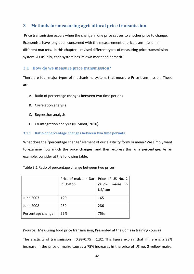
Table 3.1 Ratio of percentage change between two prices
Price of maize in Dar in US/ton
Price of US No. 2 yellow maize in US/ ton
June 2007 120 165
June 2008 239 286
Percentage change 99% 75%
(Source: Measuring food price transmission, Presented at the Comesa training course)
The elasticity of transmission = 0.99/0.75 = 1.32. This figure explain that if there is a 99%
increase in the price of maize causes a 75% increases in the price of US no. 2 yellow maize,
33
then price transmission elasticity is 1.32 (a 1.32% increase in price of maize for each 1%
increase in price of US No. 2 yellow maize)
This method is highly criticized because it only uses two points in time, does not take trends
into account (Minot et al. 2010).
3.1.2 Correlation analysis
In non-technical language, correlation exists when two variables display linear relationship
beyond what is expected by chance alone (Stockwell, 2008). When examining data in
statistical analysis, correlation reveals itself by the relationship between two variables. The
most common measure of correlation is called the “Pearson Product-Moment Correlation
Coefficient”. It is important to note that while more than two variables can be analyzed when
looking for correlation, the correlation measure only applies to two variables at a time
(Stockwel et al, 2008). Correlation is defined by most statisticians as
“A measure of the strength of relationship between random variables. The population
correlation between two variables X and Y is defined as:
ρ is called the Product Moment Correlation Coefficient or simply the Correlation Coefficient. It
is a number that summarizes the direction and closeness of linear relations between two
variables. The sample value is called r, and the population value is called ρ (rho). The
correlation coefficient can take values between -1 through 0 to +1. The sign (+ or -) of the
correlation defines the direction of the relationship. When the correlation is positive (r > 0), it
means that as he value of one variable increases, so does the other. If a correlation is negative
(r < 0), it indicates that when one variable increases, the other variable decreases. This means
there is an inverse relationship between the two variables” (sas.com).
According to Stockwell, It is important to note that a correlation measure of zero does not
necessarily imply that there is no relationship between the two variables, just that there is no
linear relationship present in the data that is being analyzed ( as the sample data is drawn
from the population). It is also sometimes difficult to judge whether a correlation measure is
“high” or “low”. There are certain situations where a correlation measure of 0.3, for example,
may be considered negligible. In other circumstances, such as in the social sciences, a 0.3
34
correlation measure may suggest that further examination is needed. As with all data
analysis, the context of the data must be understood in order to evaluate any results
(Stockwell et al, 2008).
In order to determine whether two events happen at the same time or by chance, we use the
concept of statistical significant. Statistical significance is a mathematical tool used to
determine whether the outcome of an experiment is the result of a relationship between
specific factors or due to chance (wisegeek.com). Typically, in many sciences, results that
yield P ≤ 0.05 are considered borderline statistically significant, but remember that this level
of significance still involves a pretty high probability of error (5%). Results that are significant
at the P≤ 0.05 level are commonly considered statistically significant, and P≤0.005 or P≤
0.001 levels are often called "highly" significant. Remember that these classifications
represent nothing else but arbitrary conventions that are only informally based on general
research experience (statsroft.com)
Like any quantitative measurement, correlation has its advantages and disadvantages. The
Advantage is easy to calculate and understand but is it only considers the relationship
between two variables at the same time and it does not take lags in to accounts (Minot,
2010).
3.1.3 Regression analysis
Regression analysis is a statistical tool for examination of relationships between variables.
Usually, the investigator seeks to ascertain the causal effect of one variable upon another—
the effect of a price increase upon demand, for example, or the effect of changes in the
money supply upon the inflation rate. To explore such issues, the investigator assembles data
on the underlying variables of interest and employs regression to estimate the quantitative
effect of the causal variables upon the variable that they influence. The investigator also
typically assesses the “statistical significance” of the estimated relationships that is, the
degree of confidence that the true relationship is close to the estimated relationship (O.
Sykes, 2000).
There are two major types of regression analysis that are well known in statistics. These are
simple linear regression and multiple linear regression analysis. In simple linear analysis we
only consider two main basic variables, one as dependent and the other one as an
35
independent. One simple example created by Sykes is the relationship between education
and earrings. At the outset of any regression study, one formulates some hypothesis about
the relationship between the variables of interest, here, education and earnings. Common
experience suggests that better educated people tend to make more money. It further
suggests that the causal relation likely runs from education to earnings rather than the other
way around. Thus, the tentative hypothesis is that higher levels of education cause higher
levels of earnings, other things being equal (O. Sykes, 2000). A simple linear regression model
is given by the equation
y = β0 + β1 x +ε 3.2
Where β0 and β1 are unknown parameters and ε is a random variable, usually considered
normally distributed. The model equation (3.2) states that a value of y is equal to a linear
function of x plus a random quantity ε. The parameters β0 and β1 are the intercept and slope
of the regression line (stat.ufl.edu). In applications, the model is fitted to data using the
method of least squares, giving the “prediction” equation
y = β0 + β1 x + ε 3.3
Where β0 and βError! Bookmark not defined.^1 are estimates of β0 and β1 and y is a
“predicted value” of y obtained by inserting a value of x into the prediction equation
(stat.ufl.edu).
In multiple regression analysis, the general purpose (the term was first used by Pearson,
1908) is to learn more about the relationship between several independent or predictor
variables and a dependent or criterion variable (statsoft.com). In the above Sykes example,
earnings are affected by a variety of factors in addition to years of schooling; consider the
introduction into the earnings analysis of a second independent variable called “experience”.
Holding constant the level of education, we would expect someone who has been working
for a longer time to earn more (O. Sykes, 2000).
A multiple linear regression model with k independent variables has the equation
y = β0 +β1x1 +...+βk xk +ε 3.4
36
ε is a random variable with mean 0 and variance σ2. A prediction equation for this model
fitted to data is
y = b0 + b1 x1 +... + bk xk +ε 3.5
Where y denotes the “predicted” value computed from the equation, and bi denotes an
estimate of βi (stat.ufl.edu).
Concerning price transmission, most of the previous study uses simple correlation coefficient
(Minot, 2010). A high correlation coefficient is evidence of co-movement and often
interpreted as a sign of an efficient market. Another early approach was to use regression
analysis on contemporaneous prices, with the regression coefficient being a measure of the
co-movement of prices. For example, Mundlak and Larson (1992) estimate the transmission
of world food prices to domestic prices in 58 countries using annual price data from the FAO.
They find very high rates of price transmission: the median elasticity of transmission was
0.95, implying that 95% of any change in world markets was transmitted to domestic
markets.
The static regression approach has been criticized for assuming instantaneous response in
each market to changes in other markets. In fact, there is generally a lag between the price
change in one market and the impact on another market due to the time it takes traders to
notice the change and respond to it. A change in world prices may take more than a month to
be reflected in domestic prices. These dynamic effects can be captured by including lagged
world prices as explanatory variables in the regression analysis (Ravallion, 1986; Timmer,
1987).
The advantages and the disadvantage of using multiple linear regression analysis in price
transmissions are
Advantage
- Gives information to calculate transmission elasticity
-Can test relationships statistically
-Can take into account lagged effects, inflation, and seasonality;
- Can analyze the relationship of greater than two prices,
37
Disadvantages
- Awkward to do in Excel (easier with STATA or Statistical Package for the Social Sciences (SPSS))
- Misleading results if data are non-stationary regression analysis. (Minot 2010),
3.1.4 Co-integration analysis
Cointegration theory is definitely the innovation in theoretical econometrics that has created
the most interest among economists in the last decade. The definition in the simple case of 2
time series Xt and Yt, that are both integrated of order one (this is abbreviated I(1), and
means that the process contains a unit root),
Definition:
A vector of I(1) variables yt is said to be cointegrated if there exist at vector βi such that��� iyt
is trend stationary. If there exist r such linearly independent vectors βi , i= 1,...,r, then yt is
said to be cointegrated with cointegrating rank r. The matrix β = (β1, . . . βr) is called a
cointegration matrix ( Bent, 2005). The main concept of Cointegration (Granger, 1981) and
the estimation of Cointegration give us a framework for estimating and testing for long run
equilibrium relationships between non-stationary variables (inter alia Engle and Granger,
1987; Johansen, 1988, 1991, 1995).
A time series is said to be stationary if there is no systematic change in mean (no trend), if
there is no systematic change in variance and if strictly periodic variation have been removed
(Chatfield, 2004). On the other hand, a non-stationary series has statistical property which is
time dependent. Non-stationary series may contain stochastic or deterministic trends.
Consider two prices, p1t and p2t contain stochastic trends and are integrated of the same
order, say I(d), and the two prices are in spatially separated market, then the price are said to
be cointegrated if
P1t - βP2t = µt 3.6
38
Where β is referred to as the cointegrating vector, whilst equation (3.6) is said to be the
cointegrating regression. The above equation can be estimated by utilizing inter alia Ordinary
Least Squares (OLS) (Granger, 1987) or a Full Information Maximum Likelihood method
developed by Johansen (1988, 1991). The main concept of Cointegration is that, in the long
run these prices are closely moving together, even if there may be a drift apart in the short
run, and this is consistent with the idea of market integration. Engle and Granger test the null
of no Cointegration by applying unit root tests on ût. Johansen derived the distribution of two
test statistics for the null of no cointegration referred to as the Trace and the Eigenvalue tests
(FAO, 2003).
As µt is stationary, these prices have a trend in the long run proportionality; β measures the
long run relationships between the two prices. According to Balcombe and Morrison (2002),
this measurement has sometimes referred to as the elasticity of price transmission; this is
when the prices are converted to logarithms. On the other hand, this cointegrating
parameter does not identify this elasticity, or in other words, the completeness of
transmission.
Besides testing market integration, the general idea of Cointegration has an important
implication, alleged by the Granger Representation Theorem (Engle and Granger, 1987).
According to this theorem, if two trending, say I(1), variables are cointegrated, their
relationship may be validly by an Error Correction Model (ECM), and vice verse. In the case
that prices from two spatially separated markets, p1t and p2t, are cointegrated, the Vector
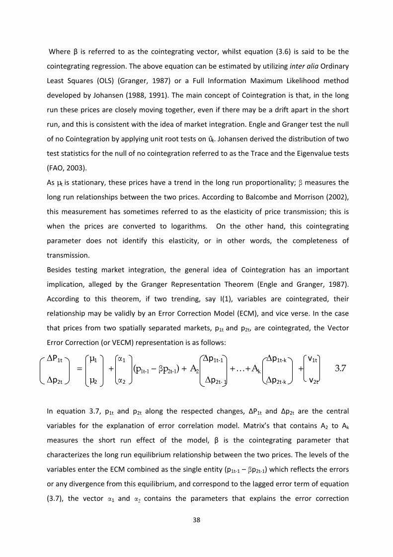
Error Correction (or VECM) representation is as follows:
∆P1t µ1 α1 ∆p1t-1 ∆p1t-k v1t = + (p1t-1 – βp2t-1) + A2 +…+Ak + 3.7 ∆p2t µ2 α2 ∆p2t- 1 ∆p2t-k v2t In equation 3.7, p1t and p2t along the respected changes, ∆P1t and ∆p2t are the central
variables for the explanation of error correlation model. Matrix’s that contains A2 to Ak
measures the short run effect of the model, β is the cointegrating parameter that
characterizes the long run equilibrium relationship between the two prices. The levels of the
variables enter the ECM combined as the single entity (p1t-1 – βp2t-1) which reflects the errors
or any divergence from this equilibrium, and correspond to the lagged error term of equation
(3.7), the vector α1 and α2 contains the parameters that explains the error correction
39
coefficient and usual between 0 < /α/ <1, i= 1,2, and it measures the extent of corrections of
the errors that the market initiates by adjusting p1t and p2t towards restoring the long run
equilibrium relationship. We can see the speed of αi(it is near to one or not) to judge whether
the market returns to its equilibrium, according to this statement short run adjustments are
directed by, and consistent with, the long run equilibrium relationship. This give a chance to
the observer to determine the speed of adjustment that shapes the relation between the two
prices (fao.org). Another important point about Cointegration is the concept of causality.
Granger (1987) explains that if there is a Cointegration between two time series, causality will
exist at least in one direction. The idea of causality testing has been used by economic
historians interested in the industrial revolution, for instance Hatton and Lyons (1983)
consider export-led growth, and Tsoulouhas (1992) the link between population and
technology. However without cointegration causality tests may yield spurious results. Engle
and Granger (1987), prove that;
“If two series are individually I(1), and cointegrated, a causal relationship will exist in at least
one direction. Furthermore, the Granger representation theorem demonstrates how to model
cointegrated I(1) series in the form of a vector autoregressive model (VAR) model. In
particular, the VAR can be constructed either in terms of the levels of the data, the I(1)
variables; or in terms of their first difference, the I(0) variables, with the addition of an error
correction term (ECM) to capture the short-run dynamics. If the data are I(1) but not
cointegrated, causality tests cannot validly be derived unless the data are transformed to
induce stationary which will typically involve tests of hypotheses relating to the growth of
variables” ( Les and Greasley, pp 1389)
The above definition has results significant dispute in the literature (Pagan, 1989) as it really
shows precedence, rather than instantaneous causality that the majority of economists
profess. However, if there is an integration between the two markets, the price in one
market, p1, would commonly be found to Granger-cause the price in the other market, p2
and/or vice versa. Thus, Granger Causality gives us additional evidence weather or in which
direction price transmission is occurring between two series. We here seriously note the
following.
40
“Granger causality may exist, indicating that, although the two price series drift apart due to
other factors such as non-stationary transaction costs, some price signals are passing through
from one market to another. On the other hand, lack of Granger causality may not imply an
absence of transmission, as price signals may be transmitted instantaneously under special
circumstances” (fao.org).
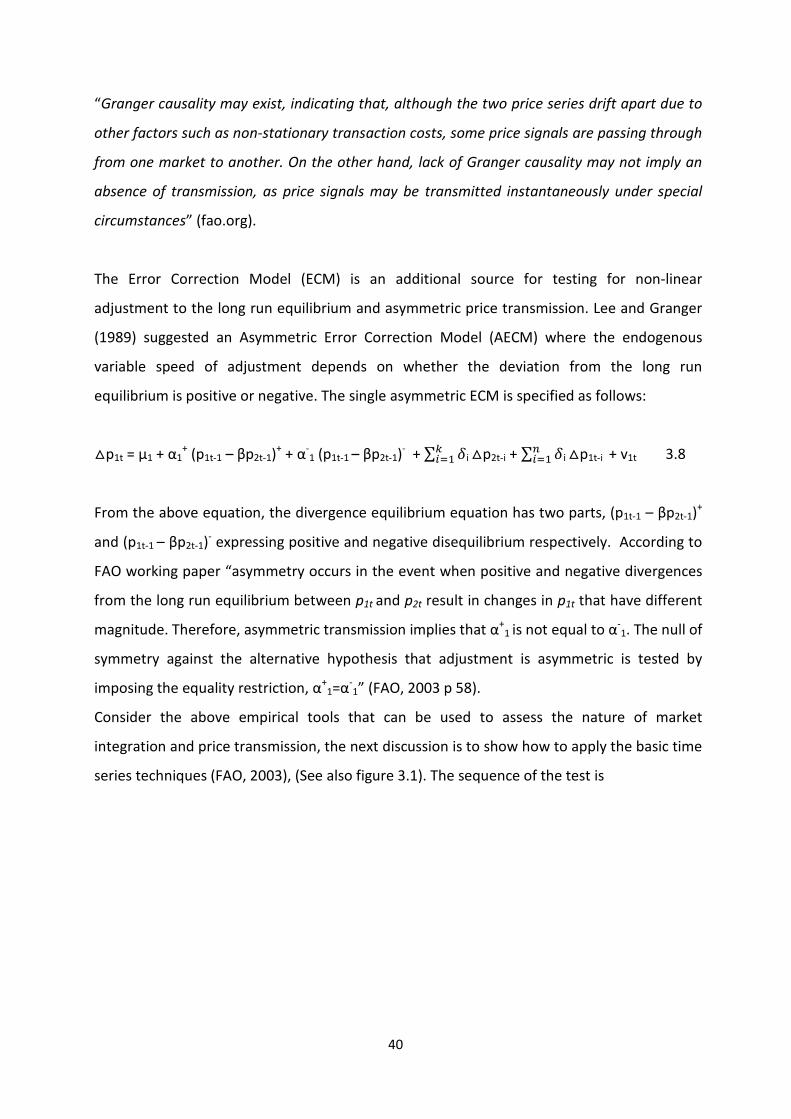
The Error Correction Model (ECM) is an additional source for testing for non-linear
adjustment to the long run equilibrium and asymmetric price transmission. Lee and Granger
(1989) suggested an Asymmetric Error Correction Model (AECM) where the endogenous
variable speed of adjustment depends on whether the deviation from the long run
equilibrium is positive or negative. The single asymmetric ECM is specified as follows:
�
△p1t = µ1 + α1+ (p1t-1 – βp2t-1)+ + α-
1 (p1t-1 – βp2t-1)- + � ��� i △p2t-i + � ��
� i △p1t-i + v1t 3.8
From the above equation, the divergence equilibrium equation has two parts, (p1t-1 – βp2t-1)+
and (p1t-1 – βp2t-1)- expressing positive and negative disequilibrium respectively. According to
FAO working paper “asymmetry occurs in the event when positive and negative divergences
from the long run equilibrium between p1t and p2t result in changes in p1t that have different
magnitude. Therefore, asymmetric transmission implies that α+1 is not equal to α-
1. The null of
symmetry against the alternative hypothesis that adjustment is asymmetric is tested by
imposing the equality restriction, α+1=α-
1” (FAO, 2003 p 58).
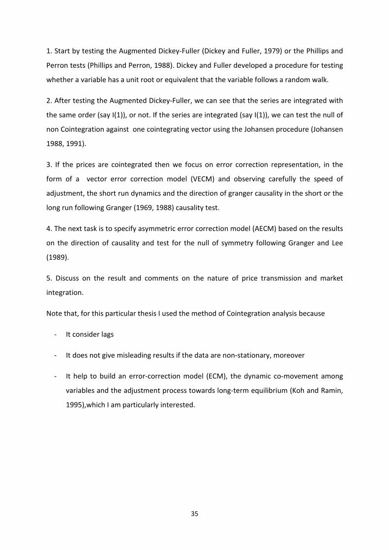
Consider the above empirical tools that can be used to assess the nature of market
integration and price transmission, the next discussion is to show how to apply the basic time
series techniques (FAO, 2003), (See also figure 3.1). The sequence of the test is
41
Figure 3.1 cointegration and vector error correction model.
if not same
test for the order of integration of the price
series (ADF, Phillips Perron)
if I(1)
if I(0)
conclude absence of
integration, perform
Granger causality tests
test the null of no cointegration between estimate ADL, perform tests for Granger
prices at different markets or levels of the Causality
supply chain (Johansen or Engle and
Granger procedures) accept
reject
perform tests for Granger Causality
specify and estimate (V)ECM, assess dynamics and speed of adjustment, test
long run Granger causality
specify and estimate AECM or include dummy for +/- disequilibria and test for
asymmetric price response and transmission
assess overall transmission and market integrat
42
Source: FAO working paper 2003
35
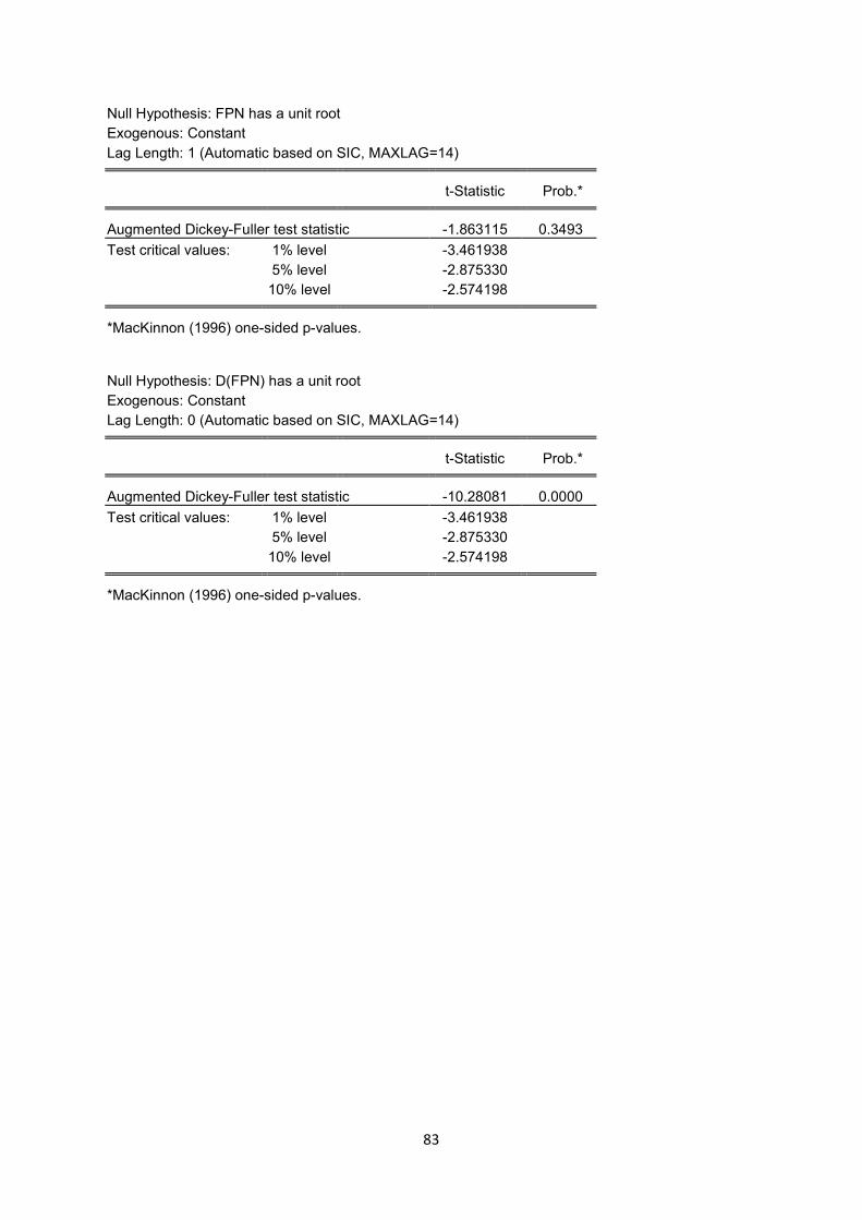
1. Start by testing the Augmented Dickey-Fuller (Dickey and Fuller, 1979) or the Phillips and
Perron tests (Phillips and Perron, 1988). Dickey and Fuller developed a procedure for testing
whether a variable has a unit root or equivalent that the variable follows a random walk.
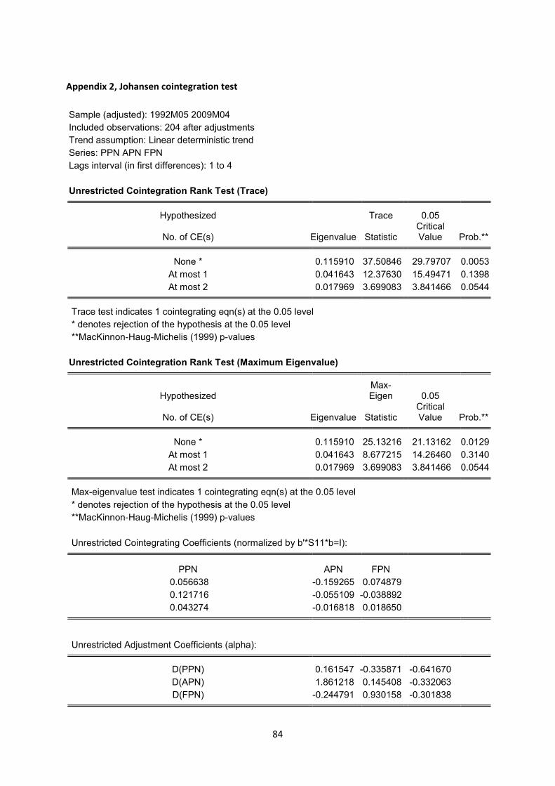
2. After testing the Augmented Dickey-Fuller, we can see that the series are integrated with
the same order (say I(1)), or not. If the series are integrated (say I(1)), we can test the null of
non Cointegration against one cointegrating vector using the Johansen procedure (Johansen
1988, 1991).
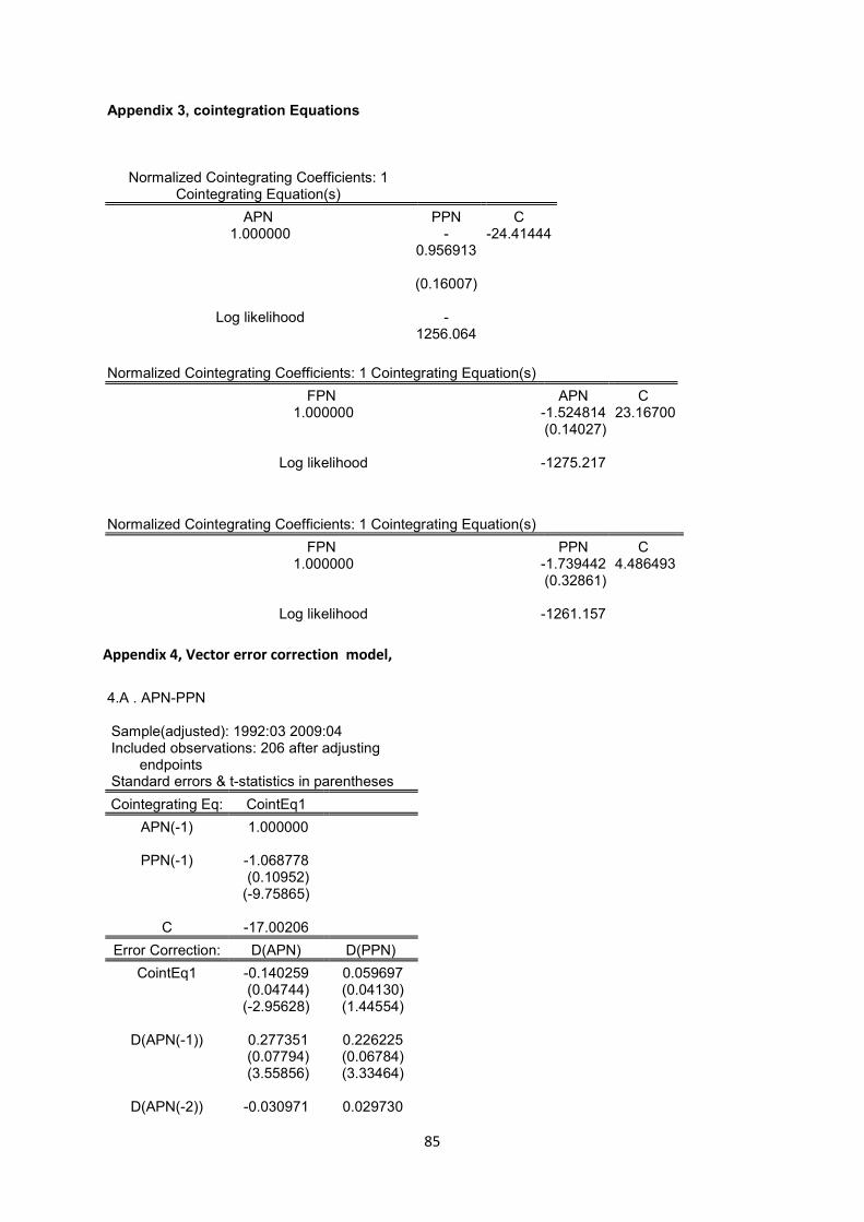
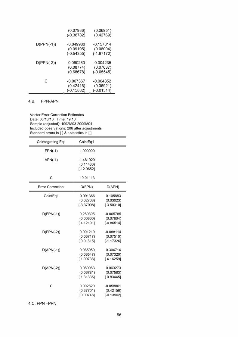
3. If the prices are cointegrated then we focus on error correction representation, in the
form of a vector error correction model (VECM) and observing carefully the speed of
adjustment, the short run dynamics and the direction of granger causality in the short or the
long run following Granger (1969, 1988) causality test.
4. The next task is to specify asymmetric error correction model (AECM) based on the results
on the direction of causality and test for the null of symmetry following Granger and Lee
(1989).
5. Discuss on the result and comments on the nature of price transmission and market
integration.
Note that, for this particular thesis I used the method of Cointegration analysis because
- It consider lags
- It does not give misleading results if the data are non-stationary, moreover
- It help to build an error-correction model (ECM), the dynamic co-movement among
variables and the adjustment process towards long-term equilibrium (Koh and Ramin,
1995),which I am particularly interested.
36
4 Mathematical formulation of coffee price in Ethiopia
In the literature review section, the law of one price is discussed, which states that when one
price is converted to a common currency, the same good should sell for the same price in
different markets. Samuelson also defines the Spatial Equilibrium Model, as the models
solving the simultaneous equilibrium of plural regional markets under the assumption of the
existence of transportation costs between two regions (Samuelson, 1951). The same model
is discussed by Enke (1951) and Takayama and Judge (1971).
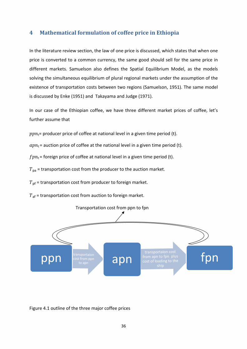
In our case of the Ethiopian coffee, we have three different market prices of coffee, let’s
further assume that
�� t= producer price of coffee at national level in a given time period (t).
�� t = auction price of coffee at the national level in a given time period (t).
�� t = foreign price of coffee at national level in a given time period (t).
�pa = transportation cost from the producer to the auction market.
�pf = transportation cost from producer to foreign market.
�af = transportation cost from auction to foreign market.
Transportation cost from ppn to fpn
Figure 4.1 outline of the three major coffee prices
ppn apn fpn
37
According to the model, “given prices for a commodity in two spatially separated markets
p1t and p2t, the Law of One Price and the Enke-Samuelson-Takayama-Judge model postulate
that at all points of time, allowing for transfer costs c, for transporting the commodity from
market 1 to market 2, the relationship between the prices is p1t = p2t + c.” (Robert 2006, pp
10)
In our case, the coffee price in auction market is equal to the producer price plus
transportation costs (see also Rapsomanikas et al. (2004), Fortenbery and Zapta (2004),
Krivonos (2004)).
�� t � �� t ���pa 4.1
Similarly, the equilibrium in coffee price between auction market and foreign market is
�� t � �� t ���af 4.2
The equilibrium in coffee price between foreign and producer price is
�� t � �� t ���pf 4.3
Assume that Rpa, Raf and Rpf are constant ratios that coffee price in two markets is attain in
equilibrium in producer – auction, auction –foreign, and producer – foreign market
respectively. (i. e. ppn/apn=Rpa, apn/fpn= Raf, ppn/fpn= Rpf) then
�� t � �� t� ��pa 4.4
�� t� �� t � �af 4.5
�� t� �� t� �pf 4.6
In the above equations, Q(4.4) to Q(4.6), Rpa, Raf and Rpf are hypothesized to be greater than
one. This is because the price in the three markets should be related as fpn > apn > ppn.
Hence, we can measure the transportation costs in the following ways from Q(4.1) to Q(4.3).
�pa� �� t����� t 4.7
�af� �� t��� t 4.8
38
�pf� �� t��� t 4.9
In the short run, the equilibrium relationships in equation (4.2) to (4.6) need not to exist due
to the incomplete transfer of information. However, they will be equilibrium relationships in
the long run.
The transfer cost in the equilibrium is the fixed ratio of the two locational prices. From our
equations (4.7), (4.8) and (4.9) , dividing these equations by apnt, fpnt and again fpnt then we
get
��a��� t = ��� t ���� t)��� t = � � �� t��� t � � � �pa 4.10 �af /�� t � ��� t ��� t)��� t� � � �� t��� t � � � �af 4.11
�pf��� t � ��� t – �� t)��� t = � � �� t��� t � � � �pf 4.12
In the literature of this paper, the equilibrium price of coffee has time series patters in
relation to Cointegration analysis ( see also Fortenbery and Zapta (2004), Krivonos (2004)).
We can write equation (4.4) to (4.6) as
�� t�� �� t ���pa 4.13
���� t = �� t���af 4.14
�� t � �� t���pf 4.15
Assume further that in equations (4.13) to (4.15), if auction price is cointegrated with
producer price, foreign price is also cointegrated with auction price and producer price with
same variable β, then
�� t – β1�� t � ��1t 4.16
��� t –β2�� t�� ��2t 4.17
�� t –β3��� t = �3t 4.18
39
Here �1t, �2t and �3t represent a stationary process with a constant mean that the two
prices are cointegrated.
According to Engle and Granger (1987), certain economic series are such that they should
not drift too far apart from each other. This means that the variables may depart from each
other in the short run, but there are certain mechanisms that force them back to a common
path after some periods. Examples of such series are, the price of a certain commodity sold
at two different locations, wages and expenditure, etc., this means that we are able to
hypothesis a long run relationships between the two coffee markets in Ethiopia. Besides this,
there exist linear combinations of the random variables that are stationary in our equation
(4.4) to (4.6) (Johansen, 1988).
We can express equations (4.13) to (4.15) in the long run to fit together by using the vector
error correction model (VAR-ECM), starting by defining the basic framework and then
considering an n – dimensional vector autoregressive error correction model. The model has
the following general form (Minot, 2010)
��t � � � ╥�t-1�� �� � k��t-k�!t 4.19
Where
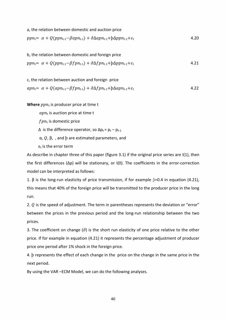
pt is an nx1 vector of n price variables, ∆is the difference operator, so pt = pt – pt-1, εt is an nx1 vector of error terms, and α is an nx1 vector of estimated parameters that describe the trend component Π is an nxn matrix of estimated parameters that describe the long-term relationship and the error correction adjustment, and Γk is a set of nxn matrices of estimated parameters that describe the short-run relationship between prices, one for each of q lags included in the model.
The vector error correction model tests for the effects of one variable on each other
variables. In our study, it measures the effect of world price to domestic price and auction
price. For our particular purpose the above equation is being simplified as
40
a, the relation between domestic and auction price
5 Source of data and estimation of error correlation model
This chapter mainly focuses on three main sub topics. The first subtopic summarizes the
sources of data; the second sub topic of this chapter examine historical price of coffee and
its volatility for two decade by considering the international coffee agreement. This gives a
broad understanding to the reader how the price looks like. Besides this, the sub topic also
includes graphical analysis of price convergence. The last part details the explanation of the
model by using econometric tools for estimating equation (4.16) to equation (4.22) that
formulated in chapter four of this study.
5.1 Source of data
The main source of data is the Central Statistical Agency of Ethiopia (CSA). The activities and
the mandate of the Central Statistical Agency (CSA) of Ethiopia are aimed at the production
of statistical data required for development planning, monitoring and evaluation of all
sectors of the economy. To achieve this, the Agency conducts several surveys to collect and
compile economic statistics in various sectors, as one of the main objectives of the CSA to
steadily develop and improve the system of economic statistics in order to extend and
intensify data collection and improve the quality of the statistical data in the country
(csa.gov.et). The producer price of coffee (�� ) was collected from a monthly survey report
by CSA. The other two price types called, auction price (�� ) and foreign price (�� ) are
from the Ministry of Agriculture and Rural Development (MOARD). This government ministry
oversees the agricultural and rural development policies of Ethiopia on a Federal level.
Foreign price refers to the price of each coffee type, which includes the value of coffee plus
cost of transportation to port including cost of loading onto ship.
Data was collected from December 1991 to April 2009 on monthly basis (around 209
observations). Four major exported coffee types have taken into consideration; these are
Sidama, Harar, Wollega and Jimma for Producer, auction and foreign price lists. (See
delimitation of the study how coffee types are selected).
43
5.2 Coffee price after 1991 in Ethiopia
The world coffee market has adramaticy change for the last twodecaded. The situation is the
same for Ethiopian coffee market, as Ethiopia is active in the world market and generates
60% of the total export earnings (Worako al el, 2008). This is because of many factorial
changes including weather, international policy environment and technological changes.
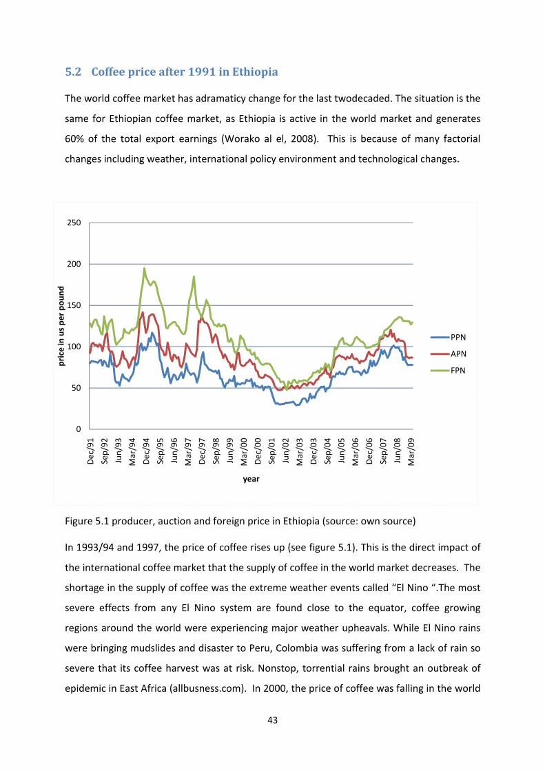
Figure 5.1 producer, auction and foreign price in Ethiopia (source: own source)
In 1993/94 and 1997, the price of coffee rises up (see figure 5.1). This is the direct impact of
the international coffee market that the supply of coffee in the world market decreases. The
shortage in the supply of coffee was the extreme weather events called “El Nino “.The most
severe effects from any El Nino system are found close to the equator, coffee growing
regions around the world were experiencing major weather upheavals. While El Nino rains
were bringing mudslides and disaster to Peru, Colombia was suffering from a lack of rain so
severe that its coffee harvest was at risk. Nonstop, torrential rains brought an outbreak of
epidemic in East Africa (allbusness.com). In 2000, the price of coffee was falling in the world
0
50
100
150
200
250
Dec
/91
Sep/
92
Jun/
93
Mar
/94
Dec
/94
Sep/
95
Jun/
96
Mar
/97
Dec
/97
Sep/
98
Jun/
99
Mar
/00
Dec
/00
Sep/
01
Jun/
02
Mar
/03
Dec
/03
Sep/
04
Jun/
05
Mar
/06
Dec
/06
Sep/
07
Jun/
08
Mar
/09
pric
e in
us
per p
ound
year
PPN
APN
FPN
44
market and reaches to its lowest real value in 100 years of history. This is because of
overproduction of coffee in the international market. In 2003, for example, 112 million to
114 million 60 kg bags of coffee were produced, compared to the 85 million bags currently
consumed (Suri, 2004). According to Oxfam (2001), more than five billion pounds of coffee
go to waste each year. Given that demand for coffee is growing very slowly while global
production continues to expand, most analysts predict that coffee’s price recovery will be
slow (Varangis et al. 2003).
From the above graph, we can see that there is a high price fluctuation in the market. In the
next sub chapter, I summarize the volatility of coffee because it helps to understand the
price fluctuates in the short as well as in the long run.
5.2.1 Coffee Price Volatility
In agricultural commodity markets, volatility is a historical word always mentioned by
economists and market makers. According to international coffee council paper 94-5,
“Volatility is a statistical measure of price fluctuations over a given period. It measures the
size of the increase or decrease in prices in a short period. It does not measure price levels but
their degree of variation from one period to the next. Marked volatility indicates a rapid
swing from low to high or high to low prices. In the case of coffee prices, volatility is strongly
influenced by supply and demand conditions. For coffee producers, volatility becomes a
matter of concern when there is a fall in prices or a price correction. When there is a
significant upturn in prices, it merits little attention. A highly volatile market has a higher
standard deviation, i.e. a high historical volatility. A market without pronounced price
fluctuations would be characterized by a low standard deviation and low historical volatility”
(International Coffee Council, 2005, pp 2).
There are different types of volatility, but the two most common are historical volatility,
which is the most commonly used measure. This is the simple standard deviation of previous
daily, weekly, or monthly percentage change in price. The other one is implied volatility,
which is derived from options, and aim to predicate actual volatility (Gilbert and Brunetti,
1995).
45
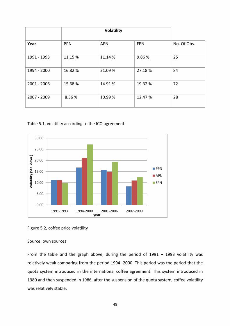
Volatility
Year PPN APN FPN No. Of Obs.
1991 - 1993 11,15 % 11.14 % 9.86 % 25
1994 - 2000 16.82 % 21.09 % 27.18 % 84
2001 - 2006 15.68 % 14.91 % 19.32 % 72
2007 - 2009 8.36 % 10.99 % 12.47 % 28
Table 5.1, volatility according to the ICO agreement
Figure 5.2, coffee price volatility
Source: own sources
From the table and the graph above, during the period of 1991 – 1993 volatility was
relatively weak comparing from the period 1994 -2000. This period was the period that the
quota system introduced in the international coffee agreement. This system introduced in
1980 and then suspended in 1986, after the suspension of the quota system, coffee volatility
was relatively stable.
0.00
5.00
10.00
15.00
20.00
25.00
30.00
1991-1993 1994-2000 2001-2006 2007-2009
Vol
atili
ty (S
ta. d
eva.
)
year
PPN
APN
FPN
46
From the period 1994 to 2000, coffee price was highly volatile. In 1997, the price reaches the
maximum level (see figure 5.1). At the end of 1997 coffee price, start declining in all markets.
The fall in the price from 1997 to 2000 was very dramatic and the lowest in real terms for
100 years. According to the ICO, the reason for this is the current imbalance between supply
and demand for coffee. Total production in coffee year 2001/02 (October-September) is
estimated at around 113 million bags (60-kg bags) while world consumption is just over 106
million bags. On top of that, world stocks amount to some 40 million bags. Coffee
production has been rising at an average annual rate of 3.6%, but demand has been
increasing by only 1.5%. At the origin of this coffee glut lies the rapid expansion of
production in Vietnam and new plantations in Brazil, which is harvesting a record crop in the
current season (ico.org). Due to the above reason the ICO come up with a new agreement in
2001, one of whose objectives is to encourage its members to develop a sustainable coffee
economy. The ICO recognizes that sustainable development has an economic and social as
well as environmental dimension. There is little doubt that the exodus from rural areas and
increased poverty in coffee producing areas caused by the current price crisis poses a very
real and wide-ranging threat to sustainable development.
Coffee price remained relatively stable from the period 2001 to 2007 comparing to 1994 to
2000 period. Finally, my test results indicate that volatility, measured based on monthly
price variations, is relatively weak from the period 2007 to 2009 (see table 5.1).
From this analysis, we can see that coffee price volatility mainly influenced by supply and
demand. The supply situation was influenced by some exogenous factors like climatic
conditions in supplying countries. (El Nino, drought, floods). On the demand side, as all the
demand comes from the developed world, the economic and industrial situations in
developed countries looks the main factors. The ICO is also playing a vital role in stabilizing
the volatility by introducing and suspending quota system, by using sustainable coffee
economy ideas, using intergovernmental consultations, increasing transparency and the
access to information.
5.2.2 Graphical analysis of price convergence
In the literature on market integration and the Law of One Price, the term “price
convergence” is often discussed. However, there is a potential risk of confusion concerning
47
what is actually meant by “price convergence”, since there is a lack of terminology
consistency in the literature. Generally, two forms of price convergence may be
distinguished: short run price convergence and long run price convergence. In brief, the
difference between the two is whether two regional markets are integrated (in the sense
that if transaction costs decrease over time and/or there is a better signal for optimal
decision) or whether they are moving towards market integration (Gluschenko, 2005).
Short run convergence
The first of the two forms of price convergence concerns the case where two regionally
separated areas, e.g. A and B, are part of the same market, i.e. the two markets are
integrated. If this is the case, the price of a certain good in region A cannot diverge limitlessly
from the price of the same good in the region B. If the price difference should ever increase
to more than the cost of transporting the good between the regions, arbitrage mechanisms
will cause this difference to disappear.
Long run price convergence
Long run price convergence is the process towards the integration of two separated
markets. Long-run convergence entails a gradually narrowing gap between the prices in
different regions. Studies of long run price convergence have its methodological origins in
development economics and studies of economic growth (Durlauf & Quah, 1999). In these
cases, whether or not incomes in different regions are converging has been the key research
question. However, the methodology and the concepts are well suited for the studies of
long- run convergence of prices as well and have been used for this purpose in a number of
studies (Ramírez, 1999; Gluschenko, 2005; Robinson, 2007). The econometric techniques for
determining whether variables have converged over time have mainly applied to cross-
country studies in real income convergence (Sala-I-Martin, 1995; Baumol and Wolff, 1986).
To get an initial idea on whether coffee prices have converged in our three different
markets, I consider the concept, which was developed by Constantin (2005). If for example
we consider producer (PPN) and auction (APN) markets, the short run convergence can be
expressed as �� t – �� t � ' where t=0…T and the long run convergence also illustrated as
()*�+,� �� t��� t)� ' (see also Constantin, 2005).
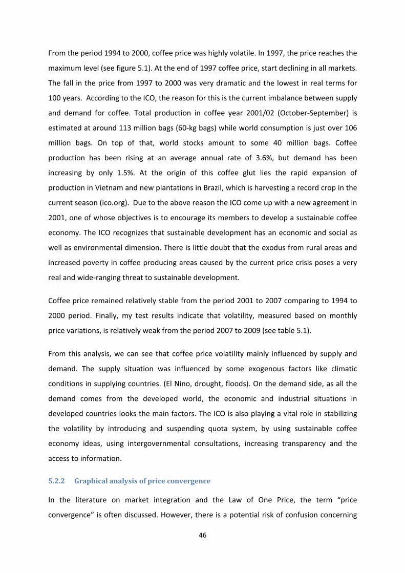
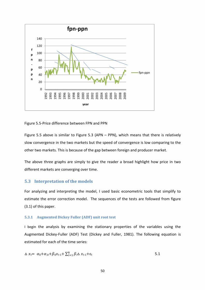
Figure 5.3 price differences between APN and PPN
In Figure 5.3, the small negatively sloped lines show as a short run convergence while the
long negatively sloped line represents the long run price convergence between the two
markets. We can clearly see from the graph that the difference between the two
become converged over time
the Ethiopian coffee industry because, the government proposes a law (Pro.No.99/1998)
that consolidation of all the taxes and duties levied on the coffee exporters into a single tax
family, abolishing of the quota system at auction, allowing private traders to trade washed
coffee, suppliers and exporters to sell coffee
0
10
20
30
40
50
60
70
80
apn-ppn
48
between APN and PPN
, the small negatively sloped lines show as a short run convergence while the
long negatively sloped line represents the long run price convergence between the two
We can clearly see from the graph that the difference between the two
in the long run since 1998. This year was the turning point in
the Ethiopian coffee industry because, the government proposes a law (Pro.No.99/1998)
at consolidation of all the taxes and duties levied on the coffee exporters into a single tax
family, abolishing of the quota system at auction, allowing private traders to trade washed
and exporters to sell coffee domestically at market-determined prices.
year
apn-ppn
apn-ppn
, the small negatively sloped lines show as a short run convergence while the
long negatively sloped line represents the long run price convergence between the two
We can clearly see from the graph that the difference between the two markets
the turning point in
the Ethiopian coffee industry because, the government proposes a law (Pro.No.99/1998)
at consolidation of all the taxes and duties levied on the coffee exporters into a single tax
family, abolishing of the quota system at auction, allowing private traders to trade washed
determined prices.
49
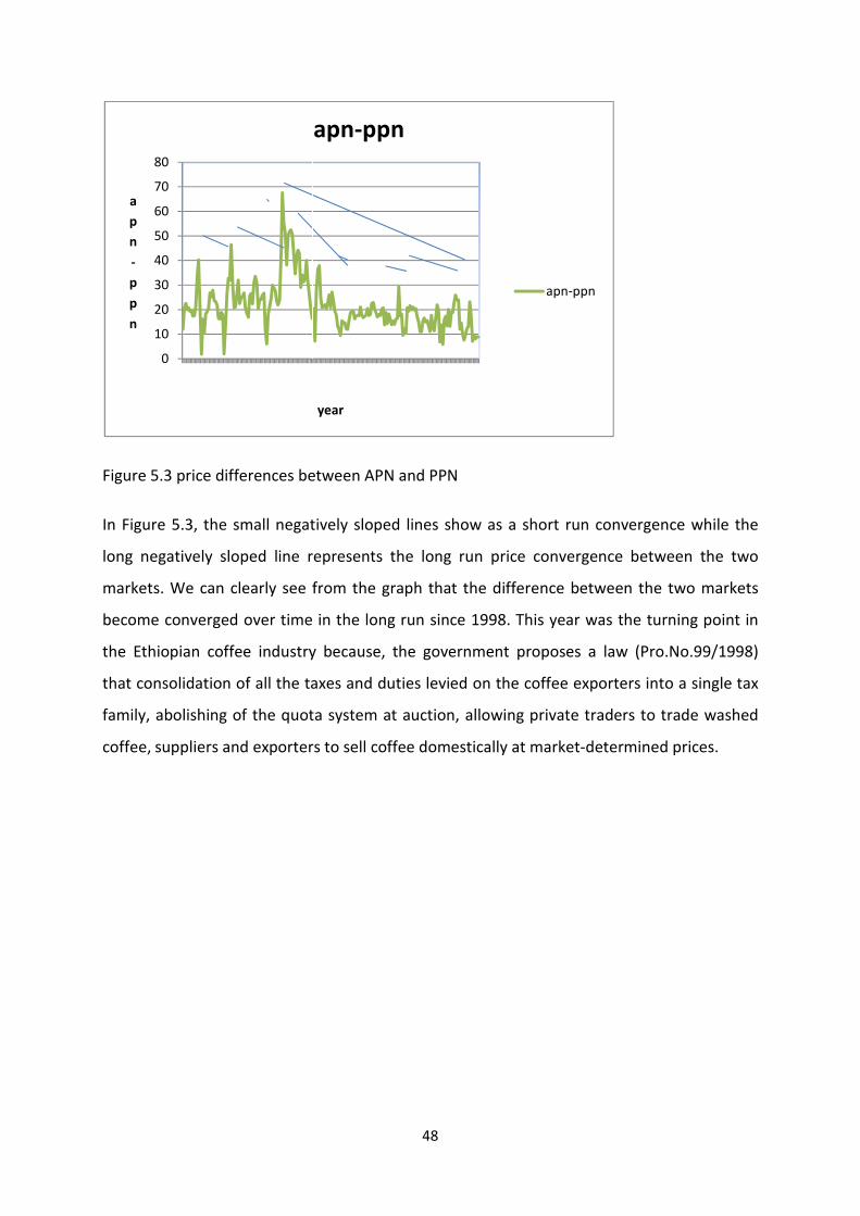
Figure 5.4-the price difference between FPN and APN
A comparison of the price difference between foreign market and auction market, (FPN –
APN) is display in Figure 5.4. The Figure indicate that even if there is an indication for price
convergence in the long run, the speed of convergence is not as fast as in the case of APN-
PPN market (compare the slope of the two graphs). According to the economics theory,
international trade in the coffee market should lead to gradual price convergence across the
international and the auction market. Remember here that what the law of one price says.
According to this law, the price of coffee in the auction market is the same as the price in the
international market allowing for the difference in the transportation costs. It is clear that
the FPN – APN market is less to converge relative to the APN-PPN market.
When we examine the price difference between foreign market and local market, we get the
following graph.
-200
20406080
100120
1992
1993
1994
1995
1996
1997
1998
1999
2000
2001
2002
2003
2004
2005
2006
2007
2008
2009
fpn-apn
year
fpn-apn
fpn-apn
50
Figure 5.5-Price difference between FPN and PPN
Figure 5.5 above is similar to Figure 5.3 (APN – PPN), which means that there is relatively
slow convergence in the two markets but the speed of convergence is low comparing to the
other two markets. This is because of the gap between foreign and producer market.
The above three graphs are simply to give the reader a broad highlight how price in two
different markets are converging over time.
5.3 Interpretation of the models
For analyzing and interpreting the model, I used basic econometric tools that simplify to
estimate the error correction model. The sequences of the tests are followed from figure
(3.1) of this paper.
5.3.1 Augmented Dickey Fuller (ADF) unit root test
I begin the analysis by examining the stationary properties of the variables using the
Augmented Dickey-Fuller (ADF) Test (Dickey and Fuller, 1981). The following equation is
estimated for each of the time series:
△ -t� ��0��1t��0-t-1�� ��� i△ -t-1�!t 5.1
0
20
40
60
80
100
120
140
1992
1993
1994
1995
1996
1997
1998
1999
2000
2001
2002
2003
2004
2005
2006
2007
2008
2009
fpn-ppn
year
fpn-ppn
fpn-ppn
51
Where Δ is the first difference operator; t is the time trend; k denotes the number of lags
used and ! is the error term; αs and βs are parameters. The purpose of the unit root test is to
determine whether the series is consistent with I (1) (integrated of order one) process with a
stochastic trend, (Nelson and Plosser, 1982) or if it is consistent with an I(0) process. That is
stationary, with deterministic trend, and still others to be integrated of order two (e.g., price
indices in some countries) ( Juselius, 1993).
Variable
name
Test on test statistics Probability decision Order of
Integration
PPN
Level -2.012030 0.2816 No rejection
І(1) First difference -15.06238 0.0000 Rejection
APN
Level -2.543525 0.1068 No rejection
І(1) First difference -11.71673 0.0000 Rejection
FPN
Level -1.863115 0.3493 No rejection
І(1) First difference -10.28081 0.0000 Rejection
Table 5.2, Augmented Dickey-Fuller Test of Unit Root (Period: 1991 to 2009)
Table 5.2, above reports the results of the Augmented Dickey-Fuller (ADF) unit root test for
PPN APN and FPN. The fact that level of the null hypothesis of the unit root cannot be
rejected when the series are in level but can be rejected when the series are in first
difference indicate that the series are integrated of order one. In all the above cases the
time series are found to be non stationary and integrated by order І(1). This means that
each variable is a random walk and integrated of the same order (I(1)). This is a necessary
but not sufficient condition for cointegration (see Granger, 1986). The next step is to carry
out co-integration analyses of the variables.
5.3.2 Testing the number of co-integration
Cointegration test is only valid the empirical data that we have is a non-stationary series. The
main purpose of the Cointegration analysis is to test whether several non stationary time
52
series data are cointegrated or not, this test will help as to determine whether a long run
relationship exists between the variables. Knowing the degree of Cointegration gives as a
basis for VEC specification (Katarzyna, 2007).
I mathematically formulate an equation (4.16, 4.17 and 4.18) by assuming that the auction
price is cointegrated with producer price, foreign price is also cointegrated with auction
price and producer price with some variable β. The estimation of these equations held here.
The software gives the Johansen test of Cointegration. Johansen proposes two different
likelihood ratio tests: the trace test (table 5.3A) and maximum eigenvalue test (table 5.3B).
Table 5.3, Cointegration test (Series: PPN APN FPN)
A. Unrestricted Cointegration Rank Test (Trace)
Hypothesized No of CE
(s)
Eigenvalue
Trace Statistic
0.05 critical value for
trace statistics
None * 0.115910 37.50846 29.79707
At most 1 0.041643 12.37630 15.49471
At most 2 0.017969 3.699083 3.841466
Trace test indicates 1 cointegrating eqn(s) at the 0.05 level
* denotes rejection of the hypothesis at the 0.05 level
B. Unrestricted Cointegration Rank Test (Maximum Eigen value)
Hypothesized No of CE
(s)
Eigen value
Trace Statistic
0.05 critical value
for trace statistics
None * 0.115910 25.13216 21.13162
At most 1 0.041643 8.677215 14.26460
At most 2 0.017969 3.699083 3.841466
Max-eigenvalue test indicates 1 cointegrating eqn(s) at the 0.05 level
* denotes rejection of the hypothesis at the 0.05 level
**MacKinnon-Haug-Michelis (1999) p-values
The trace test indicates that there is 1% significance Cointegration equation (table 5.3A), as
the same time, the maximum eigenvalue test indicate also that there is one Cointegration
53
equation between the three variables (table 5.3B). Here we notices that both trace test and
Max –eigenvalue test agree. Due to the result of these two tests, we can conclude that there
is a long-term relationship between producer, auction and foreign prices; hence, the three
prices are conjugated in the long run.
Since the long-run cointegrating relation found among the three variables, the estimation of
cointegrating vectors is executed at the same time (equations 4.16, 4.17 and 4.18 of chapter
4). The value of the cointegrating vectors (β) for auction and producer market is as follows.
Table 5.4, Cointegration vector of APN- PPN (equation 4.16 in chapter 4)
One Cointegrating Equation Log likelihood -1254.61 Normalized cointegrating Coefficients (standard error in parentheses)
APN PPN ��
1.000 0.956 (0.16) -24.41 According to table 9, we can derive a cointegrating equation between the auction price and producer price as follows, �� � './01�� � 23.3� 5.2
The Cointegration equation above suggests that a 10% permanent increase in the level of
producer price results from an increase in the auction price by 9.56%. This indicates that the
auction market is strongly co-integrated with the producer market in the long run. The value
of the cointegrating vector (� ) for foreign price and auction price in the long-run is also
estimated as,
Table 5.5, Cointegration vector of FPN-APN (equation 4.17 in chapter 4)
One Cointegrating Equation Log likelihood -1273.64 Normalized cointegrating Coefficients (standard error in parentheses)
FPN APN ��
1.000 1.523 (0.14) 23.16
According to table 10, the Cointegration between foreign price and auction price is
�� � �.04�� � 24.�1 5.3
According to equation 5.3, it is clear that a 10% permanent increase in the level of auction
price will result from a 15.3% change increase in the level of foreign price. This equation
54
indicates that even if there is a long run cointegration between foreign and auction market,
the integration is relatively weaker than the producer auction market. (the above equation
can also written as,��� � '.10�� � �0.�4, which means that if FPN increase by 10%, APN
will only increase by 6.5% in the long run.)
Similarly, the value of cointegration vectors (�) between foreign price and producer price in
the long run is estimated as,
Table 5.6, Cointegration vector of FPN-PPN (equation 4.17 in chapter 4)
One Cointegrating Equation Log likelihood 1279.01 Normalized cointegrating Coefficients (standard error in parentheses)
FPN PPN ��
1.000 1.739 (0.329) 4.486
From table 5.6, by using the estimator of Cointegration vector we can drive the
Cointegration equation between the foreign and producer price as,
�� � �.54/�� � 3.361 5.4
The equation above suggests that 10% permanent increase in the level of producer price will
results from a 17.39% change increase in the level of foreign price. This Cointegration
equation prove that the long run Cointegration between foreign and producer market is the
weakest of all the three cases (The above equation can also written as������ � '.05�� �
2.06, a 10% permanent increase in foreign market has only 5.7% impact on producer market
in the long run).
5.3.3 The Granger Causality test
Granger causality implies there exist a relation between the current value of one variable
and the past values of others (Granger, 1986). If past X contains useful information (in
addition to the information in past Y) to predict future Y, we say X “Granger causes” Y. It
does not mean changes in one variable cause changes in another. By using n-test jointly, test
for the significance of the lags on the explanatory variables, this in effect ‘Granger causality’
test between these variables. It is possible that causality exists from variable X to Y, but not Y
to X; from Y to X, but not X to Y and from both Y to X and X to Y. Although in the
interpretation of the relationship is difficult. The ‘Granger causality’ test can also be used as
55
a test for whether a variable is exogenous. I.e. if variable in the model affect a particular
variable; it can be viewed as exogenous.
Table 5.7, the granger causality test of PPN, APN and FPN
Null Hypothesis F-Statistic Probability
PPN does not Granger Cause APN 1.66526 0.14480
APN does not Granger Cause PPN 5.24274 0.00015
FPN does not Granger Cause APN 1.93670 0.08999
APN does not Granger Cause FPN 7.90805 8.5E-07
FPN does not Granger Cause PPN 0.72394 0.60622
PPN does not Granger Cause FPN 4.89141 0.00031
When we test Granger causality of producer and auction market, we cannot reject the
hypothesis that the producer price does not Granger causes the auction price, but we do
reject the hypothesis that auction price does not Granger cause producer price. Therefore, it
appears that Granger causality runs one way here from auction to producer, and not on the
other way. This evidence suggested that, in order to predict the price of future auction
market, we need to depend on the producer price but not visa verse. Note the following
that, if two variables have a common trend, Granger causality must exist in at least one
direction, unidirectional or bidirectional (Granger, 1986, 1988). Even if Cointegration
indicates the absence or present of Granger causality, it does not indicate the direction of
causality between variables. This direction of the Granger (or temporal) causality can be
detected through the VECM derived from the long run cointegrating vectors (Mansur &
Masih, 2002) (see section 5.2.4 and 5.2.5 below).
Furthermore, we cannot reject the hypothesis that foreign price does not Granger Causes
auction price (0.08 is too small to reject especially when we use lag 4) and as the same time
we do not reject the hypothesis that auction price does not Granger cause foreign price.
56
Therefore, it appears that Granger causality runs from auction to foreign and from foreign to
auction. This indicates that it is possible to predict the auction market by analyzing price in
foreign national market or, to predicate the foreign national market by depending on the
auction market.
When we compare the Granger causality between the foreign market and producer market,
we reject the null hypothesis that foreign market does not granger causes producer price,
but we cannot reject the null hypothesis that producer price does not granger causes foreign
price. Therefore, granger causality runs from producer market to foreign market but not vice
versa. Note that the term “granger causality “is something of a misnomer since a finding of
causality does not mean that movement in one variable physically causes movement in
another (Chris, 2002). In the above analysis if, for example, movements in the domestic
market (PPN) found to Granger cause movement in the foreign market (FPN), this would not
imply that the foreign market change as a direct result of, or because of movement in the
domestic market (PPN). Rather causality simply implies that a chronological order of
movement in the series.
5.3.4 Estimation of vector error correction model (VEC)
Short run integration test can be incorporated in the model by specifying a Vector Error
Correction Model (VECM) when long–run integration is observed. A vector error correction
(VEC) model is a restricted vector autoregressive (VAR) designed for use with non-stationary
series known to be cointegrated. The VEC has Cointegration relations built into the
specification so that it restricts the long-run behavior of the endogenous variables to
converge to their Cointegration relationships while allowing for short-run adjustment
dynamics (Krishna, 2010). The Cointegration term is known as the error correction term
since the deviation from long-run equilibrium is corrected gradually through a series of
partial short-run adjustments.
In chapter four of this study (equation 4.20 to 4.22) estimation has done about the vector
error correction model that helps to test the effect of each variable on each other variables.
In these equations, I specify the short-run dynamics of producer, auction and foreign
variables in the system and in a framework, which anchors the dynamics to long-run
57
equilibrium relationships. For instance, economic theory suggests that economic activity
across regions should converge. If this convergence hypothesis is true, we might observe
long-run relationships between producer, auction and foreign price.
Table 5.8. Vector error correction estimation of APN-PPN
Tweeten, L.G. and C.L. Quance, (1969) “Positivistic Measures of Aggregate Supply
Elasticities: Some New Approahces.” Amer. J. of Agr. Econ. 51:342-352.
Varangis, P., P. Siegel, D. Giovannucci, and B. Lewin, (2003). “Dealing with the coffee crisis in
Central America: impacts and strategies.” Policy research working paper 2993, World Bank,
Washington, D.C.
Ward, R. W. (1982). “Asymmetry in retail, wholesale, and shipping point pricing for fresh
vegetables.” American Journal of Agricultural Economics 62: 205-212.
Weaver, R. D., Chattin, P. and Banerjee, A. (1989). “Market structure and the dynamics of
retail food prices.” Northeastern Journal of Agricultural and Resource Economics 18: 160-
170.
Wiersum F, Gole T.W. (2008): “Certification of wild coffee in Ethiopia: Experiences and
challenges.
William Leigh (2009) “Historical Impulse Response of Return Analysis Shows Information
Technology Improves Stock Market Efficiency” University of Central Florida, College of
Business Administration, Informatica 33, 199–203.
William M. Landes and Richard A. Posner (1981) “Market power in antitrust cases” Harvard
law review, vol. 94, pp 937.
Wohlgenant, M.K., 1999. “Product heterogeneity and the relationship between retail and
farm prices.” European Review of Agricultural Economics, 26, 219-227.
Wolffram, R. (1971) “Positivisitic Measures of Aggregate Supply Elasticities – Some
NewApproaches – Some Critical Notes.” Amer. J. Agr. Econ. 53:356-359
Xiuqing Wang, Habtu Tadesse and Tony Rayner, (2006). “Price transmission, market power
and return to scale: a note.” University of Nottingham, Discussion Papers in Economics.
77
Yair Mundlak and Donald F. Larson, (1992). “On the Transmission of World Agricultural
Prices.” world bank economic reviews Volume 6, Number 3 : 399-422
Zapata, H. O. and T. R. Fortenbery (1996). “Stochastic Interest Rates and Price Discovery in selected Markets.” Review of Agricultural Markets 18: 634-654.
Zerihun Gudeta and Taddesse Kuma, (2009) “Price transmission and adjustment in the
Ethiopian coffee market.” Development Bank of Southern Africa (DBSA) & University of the
APPENDIXES Appendix 1. Unit root test of PPN, APN and FPN Null Hypothesis: PPN has a unit root Exogenous: Constant Lag Length: 0 (Automatic based on SIC, MAXLAG=14)
t-Statistic Prob.* Augmented Dickey-Fuller test statistic -2.012030 0.2816
Sample (adjusted): 1992M05 2009M04 Included observations: 204 after adjustments Trend assumption: Linear deterministic trend Series: PPN APN FPN Lags interval (in first differences): 1 to 4
Unrestricted Cointegration Rank Test (Trace) Hypothesized Trace 0.05
No. of CE(s) Eigenvalue Statistic Critical Value Prob.**
None * 0.115910 37.50846 29.79707 0.0053
At most 1 0.041643 12.37630 15.49471 0.1398 At most 2 0.017969 3.699083 3.841466 0.0544
Trace test indicates 1 cointegrating eqn(s) at the 0.05 level * denotes rejection of the hypothesis at the 0.05 level **MacKinnon-Haug-Michelis (1999) p-values
Unrestricted Cointegration Rank Test (Maximum Eigenvalue)
Hypothesized Max-Eigen 0.05
No. of CE(s) Eigenvalue Statistic Critical Value Prob.**
None * 0.115910 25.13216 21.13162 0.0129
At most 1 0.041643 8.677215 14.26460 0.3140 At most 2 0.017969 3.699083 3.841466 0.0544
Max-eigenvalue test indicates 1 cointegrating eqn(s) at the 0.05 level * denotes rejection of the hypothesis at the 0.05 level **MacKinnon-Haug-Michelis (1999) p-values
Unrestricted Cointegrating Coefficients (normalized by b'*S11*b=I):