Working Paper 22379http://www.nber.org/papers/w22379
NATIONAL BUREAU OF ECONOMIC RESEARCH1050 Massachusetts Avenue
Cambridge, MA 02138June 2016
The authors appreciate comments from seminar participants at the 2016 AERE Summer Meeting, the Beijing Institute of Technology, the 2016 NBER Spring Meeting, and the Duke Environmental Economics Workshop, as well as Gilbert Metcalf, Terry Dinan, and Roger von Haefen. The views expressed herein are those of the authors and do not necessarily reflect the views of the National Bureau of Economic Research.
NBER working papers are circulated for discussion and comment purposes. They have not been peer-reviewed or been subject to the review by the NBER Board of Directors that accompanies official NBER publications.
Prices versus Quantities with Policy UpdatingWilliam A. Pizer and Brian PrestNBER Working Paper No. 22379June 2016JEL No. D62,D92,H41,Q58
ABSTRACT
This paper considers how policy updates and trading of regulated quantities over time changes the traditional comparative advantage of prices versus quantities. Quantity regulation that can be traded over time leads firms to set current prices equal to expected future prices. A government seeking to maximize net societal benefits can take advantage of this behavior with a sequence of quantity policy updates that achieves the first best in all periods. Under price regulation where current prices remain fixed until future policy changes occur, no such opportunity exists to achieve the first best, and prices are never preferred. However, if we assume policy updates are driven in part by political "noise" rather than maximizing net societal benefits, the result changes and prices can again be preferred. The comparative advantage now depends the relative variance of noise shocks compared to true cost and benefit shocks. This contrasts sharply with the traditional comparative advantage that depends on the relative slopes of marginal costs and benefits. Applied to climate change, we estimate the comparative advantage of intertemporally tradable quantities (over prices) to be $2 billion over five years. This estimate grows if updates occur less frequently or could be made negative by political noise.
William A. PizerSanford School of Public PolicyDuke UniversityBox 90312Durham, NC 27708and [email protected]
This paper considers how policy updates and trading of regulated quantities over timechanges the traditional comparative advantage of prices versus quantities. Quantity regula-tion that can be traded over time leads firms to set current prices equal to expected futureprices. A government seeking to maximize net societal benefits can take advantage of thisbehavior with a sequence of quantity policy updates that achieves the first best in all periods.Under price regulation where current prices remain fixed until future policy changes occur,no such opportunity exists to achieve the first best, and prices are never preferred. However,if we assume policy updates are driven in part by political “noise” rather than maximizingnet societal benefits, the result changes and prices can again be preferred. The comparativeadvantage now depends the relative variance of noise shocks compared to true cost and ben-efit shocks. This contrasts sharply with the traditional comparative advantage that dependson the relative slopes of marginal costs and benefits. Applied to climate change, we estimatethe comparative advantage of intertemporally tradable quantities (over prices) to be $2 bil-lion over five years. This estimate grows if updates occur less frequently or could be madenegative by political noise.
1 Introduction
For more than forty years, economic thinking about the relative welfare advantage of alternativeprice and quantity regulation under uncertainty has gone something like this: When the regulatoris uncertain about costs known to firms, the difference in expected net benefits between otherwiseequivalent price and quantity policies hinges on the difference between the slopes of the marginalbenefit and cost schedules, multiplied by the variance of the cost shock (Weitzman 1974). Oneintuition is that government policy is attempting to replicate society’s expected marginal benefitsin the form of a demand schedule in the regulated market. A flat schedule (prices) works betterwhen marginal benefits are relatively flat (e.g., Pizer 2003); a vertical schedule (quantities) worksbetter when marginal benefits are relatively steep. A corollary to the Weitzman result is thatuncertainty about marginal benefits (unless correlated with costs) does not affect comparativeadvantage of the two instruments (Stavins 1996).
∗The authors appreciate comments from seminar participants at the 2016 AERE Summer Meeting, the BeijingInstitute of Technology, the 2016 NBER Spring Meeting, and the Duke Environmental Economics Workshop, aswell as Gilbert Metcalf, Terry Dinan, and Roger von Haefen.†Sanford School of Public Policy, Duke University. [email protected]‡University Program in Environmental Policy, Duke University. [email protected]
1
As we show in this paper, however, the outcomes can change significantly in a dynamic set-ting. In a model that extends Weitzman to multiple periods with policy updating, we show thatintertemporally tradable quantity regulation can always achieve the first-best outcome. Price reg-ulation can only achieve the first best in special cases and is never strictly preferred in this setting.Moreover, the comparative advantage now depends on uncertainty about both costs and bene-fits. We obtain this result despite the maintained assumption that the government sets its policyfor each period based on previous-period information, while the firm chooses its action based oncurrent-period information.
This result arises because of the interaction between policy updating and the arbitrage conditioncreated by an interteporally tradable quantity regulation. In the static model, cost shocks leadprice and quantity regulation to diverge in different ways from the first best. The same outcomeswould occur in our dynamic setting if the quantity instrument could not be traded across periods,regardless of whether policies are updated or not. With intertemporal trading, however, theopportunity to save (or borrow) regulated quantities for (or from) the next period implies anarbitrage condition between current and expected next-period prices as firms cost minimize. Abenefit-maximizing government can take advantage of this behavior with a particular strategy ofupdating the quantity regulation in order to achieve the first best. It can do this even with itsconstraint of setting policy each period based on previous-period information.
By contrast, under price regulation there is no comparable arbitrage condition. The govern-ment’s strategy of updating the price regulation can influence expectations about next-periodprices and policies, but cost-minimizing behavior by firms does not change the current-periodprice that they face. That is, if firms shift polluting activity in response to expectations aboutfuture pollution taxes, they do not affect the current pollution tax. Coupled with the assump-tion that the current-period policy is set based on previous-period information, the best that abenefit-maximizing government can do with a price policy in this setting is to achieve a second-bestoutcome similar to the result in Weitzman (1974).
Viewed another way, a dynamic policy setting can relax the information requirements needed toachieve the first-best policy. An intertemporally tradable quantity policy need not be set to achievethe first-best outcome in any particular period so long as firms expect the quantity allocation tobe adjusted appropriately in the future. Our proof requires a final period where uncertainty isfinally resolved and, in general, the regulator may need to use trading ratios to manipulate thearbitrage condition. However, in a simple two-period model without discounting, we show how thegovernment merely sets the first-best allocation in the second period plus a “top-up” for the firstperiod.
Of course it far from obvious whether policy updates to a particular regulation are alwaysdriven by society’s welfare maximization. With this in mind, our paper considers the possibilitythat the regulator’s objective deviates from society’s marginal net benefits by some amount. Thiscould reflect special interest politics, as environmental advocates or business interests hold toomuch sway over the government, or legal or other constraints. This possibility — what we mightcall uncertain political “noise” — favors price regulation as the adverse influence is at least delayeduntil the policy takes effect.
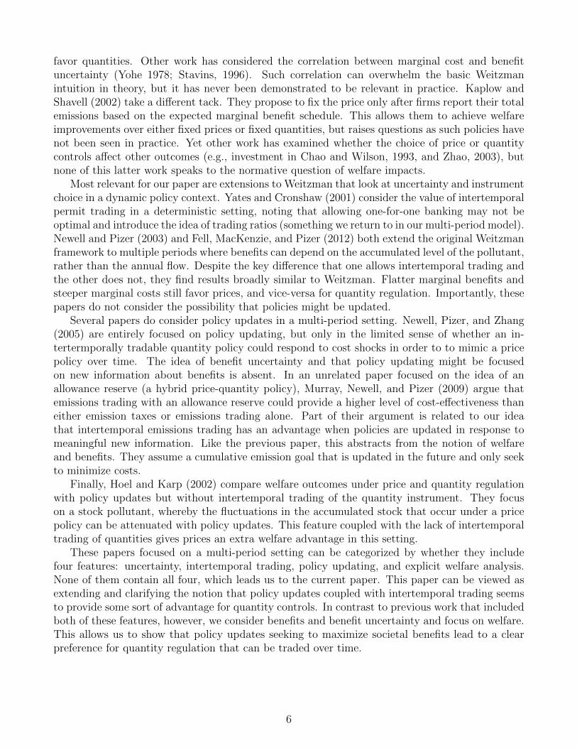
The motivation for this line of thinking stems from an attempt to explain observed outcomesunder real-world quantity regulation and to relate these outcomes to the question of comparativeadvantage. Figure 1 shows the price behavior in the SO2 trading program from 1995 through2010. Starting in 2004, future reforms to the program — a policy update in the form of the CleanAir Interstate Rule or CAIR — began to be debated. This new rule would have updated theexisting policy to reflect newer evidence of improved health benefits from lower emission levels
2
Figure 1: History of SO2 allowance spot market prices as 2010 updates were developed
(that is, higher marginal benefits of the policy). While none of the changes to the program wouldhave come into effect prior to 2010, the current (spot) price of SO2 emission permits moved inparallel to shifting expectations of future prices because of the ability to save or “bank” currentpermits for future use. Current prices adjusted to reflect the improved marginal benefit estimatesthat were to be implemented in the future, thereby achieving these higher net benefits in practicealmost immediately. Had an SO2 tax been in place, however, an expectation of a higher tax in2010 would not have influenced the current tax. This feature arguably favors quantity regulation,as the planned improvement in the policy target is realized immediately, before the change hasactually been implemented.
Starting in 2006, however, the price fell as the EPA reconsidered the proposed rules and latercourt challenges succeeded in vacating the regulation. In this case, particularly as the price fellto zero well before the new policy came into effect, an SO2 tax would have at least maintainedthe previous level of net benefits until any policy update occured. Thinking through events inthis market, one sees that the distinction between price and quantity regulation relates to theequalization of current and expected future prices under quantity regulation. The comparativeadvantage then depends on the degree to which future policy updates and prices reflect welfaremaximization or something else.
The SO2 program is far from unique in terms of intertemporal trading and policy updating.The linkage over time of markets for regulated quantities through permit banking is consistent
3
with virtually all existing tradable permit programs.1 Meanwhile, most real-world environmentalregulations are updated over time in response to new information. The 1970 Clean Air Actmakes specific provisions for the National Ambient Air Quality Standards to be updated everyfive years in response to new information (see 42 U.S. Code §7409). More recently, the EuropeanUnion announced a package of changes in their Emissions Trading Scheme, in large part owing tolow prices and (presumably) low compliance costs.2 California is similarly contemplating revisedtargets for the next phases of their program, hopefully based on improved information.3 At theU.S. federal level, in 2010 an interagency working group estimated the social cost of carbon (SCC)4
to be $24 per metric ton in 2010. That number was revised upward to $37 based on new modelingestimates of damages in 2013.5
There is a similar list of policy updates where one might question whether aggregate welfaremaximization is the main goal. These include New Jersey’s decision to exit the Regional Green-house Gas Initiative (RGGI) in May 2011, Australia’s decision to terminate their carbon pricingprogram in July 2014, and the U.S. Supreme Court decision to stay implementation of the CleanPower Plan in February 2016.
In the remainder of the paper, we first review the basic Weitzman (1974) result and otherrelevant literature. We then show how the Weitzman result changes if we allow policy updatesand intertemporal quantity trading. To illustrate our main results, we present a simple two-period model with a common shock across both periods and no discounting. After showing howintertemporally tradable quantity regulation can achieve the first best outcome, we introducethe possibility that policy updates might be driven by influences other than new informationabout costs and benefits, such as shifting special interests or evolving legal or other constraints.This reintroduces the possibility that price regulation is strictly preferred, with the comparativeadvantage determined by the magnitude of this policy noise relative to new information aboutcosts and benfits. All of these results can be generalized to multiple periods with AR(1) errorprocesses and discounting, as we demonstrate in section 5. Finally, we apply our model to the caseof global climate change, estimating that intertemporally tradable quantities provide an expectedwelfare gain over price regulation of $2 billion per five-year period, assuming policies are updatedevery five years, a number that grows if updates occur less frequently.
2 The Weitzman Result and Subsequent Work
In his seminal 1974 article, Martin Weitzman explored the difference between price and quantityregulation in a simple linear model. Assuming costs and benefits represented by
C(q, θ) = c0 + (c1 + θ)(q − q̂) + c22
(q − q̂)2 (1)
B(q, η) = b0 + (b1 + η)(q − q̂)− b22
(q − q̂)2, (2)
1This includes lead phase-down program in the 1980s, the acid rain program in the 1990s and 2000s, theEuropean Emissions Trading Scheme, California’s cap-and-trade program, among others. Most programs allowlimited borrowing.
2See http://ec.europa.eu/clima/policies/2030/index_en.htm.3See http://www.arb.ca.gov/cc/scopingplan/scopingplan.htm.4The SCC represents the marginal benefit of reducing CO2 emissions by one metric ton.5Both figures are estimated for emissions reductions occurring in 2015 and presented in 2007 dollars. See
Interagency Working Group on Social Cost of Carbon (2010) and (2013) for details.
linear marginal costs and benefits can be written as
MC(q, θ) = c1 + θ + c2(q − q̂) (3)
MB(q, η) = b1 + η − b2(q − q̂). (4)
Here, θ represents cost uncertainty while benefit uncertainty is captured in a similar way by η. Foran arbitrary q̂, the parameters c1 and c2 describe marginal costs in a flexible way, and similarlyso for b1 and b2. As in Weitzman, we assume c2 > 0 and b2 ≥ 0, MC(0, θ) < MB(0, η) andMC(q, θ) > MB(q, η) for large enough q. This implies a single first-best outcome, regardless ofwhether q is a good or a bad.6
In his paper, the linear model is described as an approximation to more general functions aboutthe point q̂ where marginal costs equal marginal benefits on average. That is, he (and we) assumeMC(q̂, 0) = MB(q̂, 0) and c1 = b1. While this assumption is not required to derive the key results,it simplifies the exposition and the expected optimal government policies. These become q̃O = q̂for quantities and p̃O = c1 = b1 for prices. Here and throughout, we use a t̃ilde over a variableto indicate a chosen government policy; the superscript O more specifically refers to the OriginalWeitzman framework for policymaking.
With this setup, Weitzman derives his main result. When price and quantity regulations areset to maximize expected net benefits, the expected welfare advantage of prices is given by
∆O =σ2θ
2c22(c2 − b2). (5)
Weitzman’s appealingly simple result (5) shows that the direction of the welfare advantage ∆O de-pends only on the relative slopes of marginal costs and marginal benefits, c2 and b2. We previouslymentioned the intuition that a price policy, filling in the otherwise absent market demand role,better matches the marginal benefit schedule when it is relatively flat (and vice-versa for quantitypolicies when the marginal benefit schedule is relatively steep). Another intuition is that priceregulation offers welfare savings because such a policy does more when costs are low and less whencosts are high. To the extent costs are convex (large c2), this improves welfare. At the same time,a price policy introduces variability into q, which is fixed under quantity regulation. To the extentbenefits are concave (large b2), variable q reduces welfare. The net effect depends on the sign ofc2 − b2. Put simply, if marginal benefits are relatively steep compared to marginal costs, thengetting the quantity “right” is important in welfare terms, implying that quantity instruments areexpected to perform better. Otherwise, price instruments are to be preferred.
The magnitude of both the expected cost saving and benefit loss depends on variability incosts — here, the variation in θ. Benefit uncertainty — variability in η — does not appear in theexpression. Benefit uncertainty does lower expected welfare, but it does so equally for price andquantity regulation.
Weitzman’s findings have been extended to many other contexts in the literature. This includesalternative forms of uncertainty (Fishelson, 1976; Yohe, 1978; Stranlund and Ben-Haim, 2008) andnon-linear marginal costs and benefits (Yohe, 1978; Kelly, 2005). In all of these cases, the basicresult generally remains that flatter marginal benefits favor prices and steeper marginal benefits
6Weitzman focuses on q as a good (e.g., clean air) for simplicity. However, our motivating example is pollutionwhere marginal benefits may be flat and where quantity controls are more easily viewed as regulating a bad (e.g.,emissions). There is nothing in the model or notation that favors one or the other, but the reader should keep inmind that for bads, marginal benefits and hence prices are negative; firms must pay rather than being paid forproducing bads.
5
favor quantities. Other work has considered the correlation between marginal cost and benefituncertainty (Yohe 1978; Stavins, 1996). Such correlation can overwhelm the basic Weitzmanintuition in theory, but it has never been demonstrated to be relevant in practice. Kaplow andShavell (2002) take a different tack. They propose to fix the price only after firms report their totalemissions based on the expected marginal benefit schedule. This allows them to achieve welfareimprovements over either fixed prices or fixed quantities, but raises questions as such policies havenot been seen in practice. Yet other work has examined whether the choice of price or quantitycontrols affect other outcomes (e.g., investment in Chao and Wilson, 1993, and Zhao, 2003), butnone of this latter work speaks to the normative question of welfare impacts.
Most relevant for our paper are extensions to Weitzman that look at uncertainty and instrumentchoice in a dynamic policy context. Yates and Cronshaw (2001) consider the value of intertemporalpermit trading in a deterministic setting, noting that allowing one-for-one banking may not beoptimal and introduce the idea of trading ratios (something we return to in our multi-period model).Newell and Pizer (2003) and Fell, MacKenzie, and Pizer (2012) both extend the original Weitzmanframework to multiple periods where benefits can depend on the accumulated level of the pollutant,rather than the annual flow. Despite the key difference that one allows intertemporal trading andthe other does not, they find results broadly similar to Weitzman. Flatter marginal benefits andsteeper marginal costs still favor prices, and vice-versa for quantity regulation. Importantly, thesepapers do not consider the possibility that policies might be updated.
Several papers do consider policy updates in a multi-period setting. Newell, Pizer, and Zhang(2005) are entirely focused on policy updating, but only in the limited sense of whether an in-tertermporally tradable quantity policy could respond to cost shocks in order to to mimic a pricepolicy over time. The idea of benefit uncertainty and that policy updating might be focusedon new information about benefits is absent. In an unrelated paper focused on the idea of anallowance reserve (a hybrid price-quantity policy), Murray, Newell, and Pizer (2009) argue thatemissions trading with an allowance reserve could provide a higher level of cost-effectiveness thaneither emission taxes or emissions trading alone. Part of their argument is related to our ideathat intertemporal emissions trading has an advantage when policies are updated in response tomeaningful new information. Like the previous paper, this abstracts from the notion of welfareand benefits. They assume a cumulative emission goal that is updated in the future and only seekto minimize costs.
Finally, Hoel and Karp (2002) compare welfare outcomes under price and quantity regulationwith policy updates but without intertemporal trading of the quantity instrument. They focuson a stock pollutant, whereby the fluctuations in the accumulated stock that occur under a pricepolicy can be attenuated with policy updates. This feature coupled with the lack of intertemporaltrading of quantities gives prices an extra welfare advantage in this setting.
These papers focused on a multi-period setting can be categorized by whether they includefour features: uncertainty, intertemporal trading, policy updating, and explicit welfare analysis.None of them contain all four, which leads us to the current paper. This paper can be viewed asextending and clarifying the notion that policy updates coupled with intertemporal trading seemsto provide some sort of advantage for quantity controls. In contrast to previous work that includedboth of these features, however, we consider benefits and benefit uncertainty and focus on welfare.This allows us to show that policy updates seeking to maximize societal benefits lead to a clearpreference for quantity regulation that can be traded over time.
6
3 Policy Updating
We now expand the earlier Weitzman model to two periods with the same, but uncertain, costsand benefits in both periods. The regulator sets the first-period price or quantity policy prior tolearning about costs and benefit uncertainty, θ and η in (1) and (2), but we consider the possibilitythat s/he sets the second-period policy once the uncertainty is known. That is, we change theinformation asymmetry to represent a lag in policy implementation in the context of evolvingknowledge rather than a perpetual difference in what may be known or unknown.
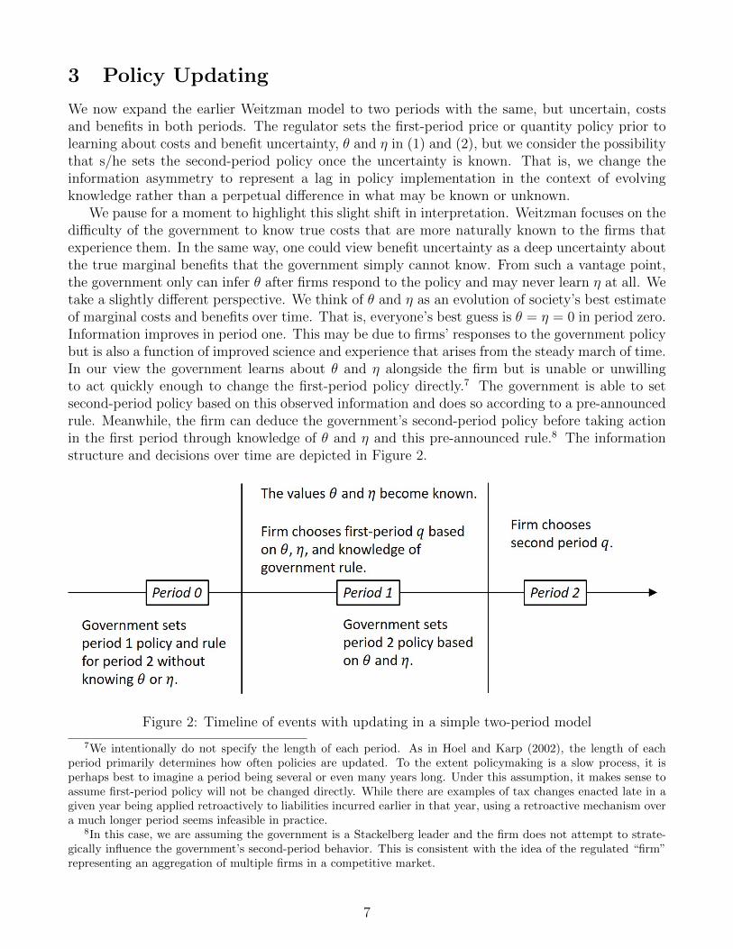
We pause for a moment to highlight this slight shift in interpretation. Weitzman focuses on thedifficulty of the government to know true costs that are more naturally known to the firms thatexperience them. In the same way, one could view benefit uncertainty as a deep uncertainty aboutthe true marginal benefits that the government simply cannot know. From such a vantage point,the government only can infer θ after firms respond to the policy and may never learn η at all. Wetake a slightly different perspective. We think of θ and η as an evolution of society’s best estimateof marginal costs and benefits over time. That is, everyone’s best guess is θ = η = 0 in period zero.Information improves in period one. This may be due to firms’ responses to the government policybut is also a function of improved science and experience that arises from the steady march of time.In our view the government learns about θ and η alongside the firm but is unable or unwillingto act quickly enough to change the first-period policy directly.7 The government is able to setsecond-period policy based on this observed information and does so according to a pre-announcedrule. Meanwhile, the firm can deduce the government’s second-period policy before taking actionin the first period through knowledge of θ and η and this pre-announced rule.8 The informationstructure and decisions over time are depicted in Figure 2.
Figure 2: Timeline of events with updating in a simple two-period model
7We intentionally do not specify the length of each period. As in Hoel and Karp (2002), the length of eachperiod primarily determines how often policies are updated. To the extent policymaking is a slow process, it isperhaps best to imagine a period being several or even many years long. Under this assumption, it makes sense toassume first-period policy will not be changed directly. While there are examples of tax changes enacted late in agiven year being applied retroactively to liabilities incurred earlier in that year, using a retroactive mechanism overa much longer period seems infeasible in practice.
8In this case, we are assuming the government is a Stackelberg leader and the firm does not attempt to strate-gically influence the government’s second-period behavior. This is consistent with the idea of the regulated “firm”representing an aggregation of multiple firms in a competitive market.
7
In addition to the assumed information structure and decision sequence, we make the furtherassumption that the quantity instrument can be traded between the two periods. As we havenoted, this is consistent with virtually all observed tradable permit systems that allow currentperiod permits to be saved, or “banked”, for use in the future and many that allow some volumeof future period permits to be used early, or “borrowed”.
We now characterize firm behavior, the government’s welfare-maximizing price and quantitypolicies, and the relative advantage of prices versus quantities, for both fixed and updated policies.
3.1 Firm Behavior
In the traditional Weitzman framework, firm behavior under a generic quantity policy q̃ was totrivially set q = q̃. Here, it is not so simple in the first period as the firm has the option to usethe assigned quantities q̃1 or to deviate, creating a bank B = q̃1 − q1. This bank can be in surplusor deficit B ≷ 0 to be made up in the second period. For that reason, we work backwards: In thesecond period, there is no option except q2 = q̃2 + B. Then, in the first period we can write thefirm’s problem as:
maxB−C(q̃1 −B, θ)− C(q̃2 +B, θ).
We ignore discounting for the moment. We also take advantage of the fact that there is nouncertainty from the perspective of the firm. It knows the cost and benefit shocks before it makesany decisions and knows the government’s optimal second-period policy based on θ and η. Thisleads to an arbitrage condition for the firm: MC(q1, θ) = MC(q2, θ). That is, equalize marginalcosts across periods. Given the same cost function in both periods, we have a simple solution:
q1 = q2 =q̃1 + q̃2
2. (6)
That is, divide the cumulative quantity regulation equally over the two periods. This is trueregardless of what kind of quantity policy (fixed or updating) is used to define q̃2.
Firm behavior under a price policy is the same as derived by Weitzman. Facing prices p̃t ineither period for output qt, firms will choose qt to maximize profits. That is,
maxqt
p̃tqt − C(qt, θ),
recalling that p̃t will be positive or negative depending on whether qt is a good or a bad. Thisleads to a simple rule for the firm: MC(qt, θ) = p̃t. That is, set marginal costs each period tothe regulated price. Given the definition of marginal costs in (3), this yields Weitzman’s responsefunction,
h(p̃t, θ) = q̂ +p̃t − c1 − θ
c2.
3.2 Optimal Price and Quantity Policies
For comparison, we first consider what happens when the government chooses its policies to max-imize expected net benefits over both periods without knowing the values of η and θ (that is,without updating). Absent updating, this replicates the earlier Weitzman policy result but nowextended over two periods, which we denote with superscript W . In the case of intertemporallytradable quantities, it is clear from equation (6) that only the total quantity volume q̃ = q̃1 + q̃2matters as a policy choice variable and the allocation between periods does not matter. Following
8
the Weitzman approach that costs and benefits are approximated around q̂ where b1 = c1, it istrivial to show that expected net benefits are maximized when the cumulative quantity is givenby q̃W = 2q̂, which could be implemented with q̃Wt = q̂ in each period. In the case of prices,the symmetry of the problem leads to the original Weitzman solution p̃Wt = c1 = b1, resulting inequilibrium quantities of q̂ − θ
c2in each period.
With updating, the government has the ability to pick q̃2 and p̃2 after observing θ and η. Inthe case of prices, this is relatively straightforward because there is no behavioral link betweenperiods and the government faces two distinct optimizations. In period one, p̃U1 = c1 leading toequilibrium quantities of q̂ − θ
c2as before, where superscript U indicates the government’s welfare
maximizing solution to the updating policy problem. In period two, we have a first-order conditionfor the optimal updating policy p̃U2 when all the uncertain outcomes are now known:(
MB(h(p̃U2 , θ
), η)−MC
(h(p̃U2 , θ
), θ))hp(p̃
U2 , θ) = 0.
Substituting and rearranging, we have
c2(θ − η) + (b2 + c2)(p̃U2 − c1 − θ) = 0,
or
p̃U2 = c1 +b2θ + c2η
b2 + c2.
This is the expression for the first-best, updated price in the second period. Note that in the secondperiod, the regulator is able to achieve the first-best outcome as there is no longer an informationasymmetry.
Optimal quantities are also straightforward. Let q̃ = q̃1 + q̃2. From the previous discussion, weknow that the firm chooses q1 = q2 = q̃/2. This is true regardless of how the government dividesq̃ between periods one and two. Therefore, the government’s problem amounts to figuring out thecumulative, two-period quantity policy q̃U to maximize net benefits:
maxq̃
[2B(q̃/2, η)− 2C(q̃/2, θ)] ,
where we let q̃U denote this optimized policy. Note that because the government can choose thesecond-period allocation after it observes the uncertain outcomes, it can determine the cumula-tive quantity target q̃ using the true values of θ and η, thereby circumventing the informationasymmetry!
as the optimal, updated quantity policy. Intuitively, the second-period allocation is the first-bestoutcome for the second period q∗ = q̂ + η−θ
b2+c2, plus a “top-up” (q∗ − q̃U1 ) to adjust the first-period
9
allocation to the first-best level. This achieves the first-best outcome in both periods (in contrastto the price policy, which only achieves the first-best outcome in the second period). That is,knowing the firm will equalize marginal costs and divide the cumulative allocation across bothperiods, the regulator adjusts the quantity policy in the second period to accommodate the first-best outcome in both periods. This suggests that the comparative advantage for the updatingpolicies will simply reflect the first-period loss under the price policy, which we now show.
3.3 Comparative Advantage
Without updating, the comparative advantage of prices versus quantities, ∆W , is simply the orig-inal Weitzman result over two periods, or
∆W = 2∆O =σ2θ
c22(c2 − b2).
With updating, both policies achieve the first-best outcome in the second period. The comparativeadvantage stems from differences in the first-period outcome, namely the loss associated with thestandard price instrument,
∆U = E[(B(h(p̃U1 , θ), η)− C(h(p̃U1 , θ), θ)
)−(B(q̃U/2, η)− C(q̃U/2, θ)
)]=−(σ2
η + (b2/c2)2σ2
θ)
2(b2 + c2). (8)
We provide an algebraic proof of (8) in the appendix, but a simple graphical proof is as follows.9
In the first period, the updating price policy is simply the standard price policy, p̃U1 = c1 and leadsto the outcome at point b in Figure 3. Meanwhile the updating quantity policy obtains the firstbest q = q̃U/2 = q̂ + η−θ
b2+c2at point c.
Whereas the quantity outcome is first best, we can see from the figure that the price policyleads to the shaded deadweight loss, DWL. This is a triangle where the “height” in the quantitydimension is θ
c2+ η−θ
b2+c2= η+(b2/c2)θ
b2+c2. The “base” along the price dimension equals the height times
b2 + c2. The area is then one-half base times height, or (η+(b2/c2)θ)2
2(b2+c2). Taking expectations of this
area yields the expressed loss in (8).
3.4 Discussion of Key Assumptions
It is clear that the price policy is never preferred in this model. The quantity policy is first bestin both periods while the price policy is generally only first best in the second period. In thespecial case where marginal benefits are flat (b2 = 0) and there is no benefit uncertainty (σ2
η = 0),the relative advantage is zero. In such a case, prices achieve the first best. Thus, quantities withupdating is weakly superior to prices. Quantities always achieves the first-best outcome and thewelfare loss from price policies depends on both cost and benefit uncertainty.
This is quite different from the Weitzman result, without updating, where the difference betweenthe marginal benefit and cost slopes determines an otherwise ambiguous preference between priceand quantity controls. Moreover, both price and quantity controls are second best in the Weitzman
9The point where the x-axis intercepts the y-axis in Figure 3 should not be interpreted as the origin. It is zerofor the x-axis but will be a negative number for the y-axis in the case of a bad. That is, this figure arises in thefirst quandrant for a good but the fourth quandrant for a bad.
10
Figure 3: Illustration of deadweight loss from price policy
framework due to the information asymmetry faced by the government. Benefit uncertainty doesnot appear in the comparative advantage expression (5) because it equally affects the expectedwelfare loss from both prices and quantities.
What’s going on? It is clear that there is an important interaction between policy updatingand intertemporal trading, both of which tend to be present in practice. We have demonstratedthat without updating and with intertemporal trading, the original Wetizman result remains inboth periods. It is similarly easy to see that without intertemporal trading and with updating, theoriginal Weitzman result remains in the first period (because the first period is just the Weitzmansetup). But these two features together lead to a different result. In this setting, if firms haveexpectations about second-period policy updates before they make choices in the first period, thepotential to trade across periods leads them to equalize current and expected future prices drivenby the expected policy update. The result must be different. But must it achieve first-best?
Several additional implicit or explicit assumptions lead to the first-best outcome. First, we makea rational expectation assumption that firms are, in fact, expecting what the government ultimatelydoes. This seems reasonable, as anything else should eventually lead to revised expectations.Second, we need to identify a quantity-policy updating rule for the government such that theexpected next-period prices indeed achieve the first-best outcome. In the simple two-period model,we made that easy by assuming the periods were identical with a single common shock and nodiscounting. We will see in section 5 that more generally, with different shocks in different periods
11
and more periods, there is still an updating rule that achieves the first-best in every period. Finally,we assume the government regularly updates policy based on societal net benefits and not someother objective. This is perhaps the most questionable assumption, to which we now turn.
4 Policy Updating with Noise
While improved cost-benefit information in future policy decisions can improve current-periodregulatory outcomes under intertemporally tradable quantity controls, what if something otherthan improved information influences future policy? It is easy to imagine policy decisions beingdriven in part by special interests and more narrowly defined benefits rather than broad, societalcosts and benefits. If we expect such changes to an intertemporally tradable quantity target in thefuture, we should be worried that these changes will be transmitted back to the present.
In particular, suppose that when the government updates its policy it acts as if marginalbenefits in (4) are subject to an additive disturbance ε reflecting uncertain special-interest politicalpressure rather than true information about societal benefits. One could also interpret this term asthe Lagrangian multiplier on uncertain legal, political, or other constraints that bound the policychoice. Put simply, suppose the government now makes use of a “noisy” marginal benefit functiongiven by
that it wishes to equate with marginal costs in order to update its policy. The function MBwithout any subscript continues to refer to true, societal marginal benefits, while MBnoisy is thedivergent, special-interest or constrained version of marginal benefits used to update policy. Forsimplicity, we assume there is no noise when policy is initially set for the first period, and ε refersto the distortion introduced in period 1 along with the other true shocks to costs and benefits. Insection 5 we extend this to an evolving noise process.
In adding this notion of political noise, we make the same information assumption about noiseas we do about the true shocks to costs and benefits. Namely, the firm has more up-to-dateinformation about the evolution of political noise than is necessarily reflected in current policy.More specifically, the government sets policy for period 1, p̃N1 or q̃N1 , before any political noise orshocks to costs and benefits occur. Here, superscript N refers to the policy chosen in our setupwith noise. By the time it acts in period 1, the firm knows the value of ε as well as θ and η thatwill be used to update policies coming into effect in period 2. At the same time or soon after, thegovernment sets p̃N2 or q̃N2 based on that same realization of θ, η, and ε.
Returning for a moment to our SO2 trading program example, firms were well aware of evolvinginformation, political forces, and legal opinions that were shaping the regulatory environment for2010 and beyond. This awareness influenced pollution behavior and permit prices beginning asearly as 2004. From 2004 to 2006, these changes were arguably driven by better informationabout welfare-improving, societal marginal benefits reflected in the initially proposed CAIR, whichsuggested such benefits were well in excess of $1600 per ton (U.S. EPA 2005). During 2006-2009, theinfluences were arguably non-welfare-improving political forces and legal decisions, as the marketprice diverged from marginal benefits. In our model terminology, consider the period 2004-2009(and earlier years going back to 1995) as an elongated period 1. This policy was established underthe 1990 Clean Air Act Amendments, which we would call period 0. During 2004-2009, firmsexpected the policy to be updated based on this period 1 information for 2010 and beyond, whichwe would call period 2.
12
Solving for the optimal price policy is relatively straightforward because the choices each periodare not linked by the firm. Choosing p̃N1 such that E[MBnoisy(h(p̃N1 , θ), η, 0)−MC(h(p̃N1 , θ), θ)] = 0,we have the government’s “optimal” price policy for period 1 as viewed in period 0. Note thatthe government is seeking to take expectations of θ and η but not ε. The value of ε — zero beforethe first period — enters directly, as the government’s current special interests or current legalconstraints are what matter for setting policy. This leads to
p̃N1 = E[p∗]. (10)
For period 2, uncertainty is revealed and noise is realized, so the government chooses p̃N2 such thatMBnoisy(h(p̃N2 , θ), η, ε)−MC(h(p̃N2 , θ), θ) = 0, or
p̃N2 = p∗ +c2ε
b2 + c2. (11)
The expression p∗ represents the first-best price outcome in terms of true aggregate net benefits,10
but the government’s objective now deviates from the goal of maximizing expected, aggregatenet benefits. Using the firm’s reaction function, which is unchanged from our basic model, theequilibrium quantity outcomes are:
q1 = h(p̃N1 , θ) = q̂ − θ
c2
= q∗ − η + (b2/c2)θ
b2 + c2
q2 = h(p̃N2 , θ) = q̂ +η − θb2 + c2
+ε
b2 + c2
= q∗ +ε
b2 + c2.
where q∗ is the first-best outcome in each period. These quantity outcomes are the same as thosein our basic model plus the noise distortions in the second period.
Under a quantity policy with updating and intertemporal trading, we know the firm will simply
set qt =q̃N1 +q̃N2
2and what matters is this cumulative allocation as before. With the revealed values
of θ and η and the realized value of ε, the government can choose q̃N2 based on an arbitrary choiceof q̃N1 such that MBnoisy = MC each period, or
b1 + η − b2(q̃N1 + q̃N2
2− q̂)
+ ε = c1 + θ + c2
(q̃N1 + q̃N2
2− q̂)
q̃N2 = 2q̂ + 2η − θb2 + c2
+ 2ε
b2 + c2+ 2
b1 − c1b2 + c2
− q̃N1
= q∗ +ε
b2 + c2+
(q∗ +
ε
b2 + c2− q̃N1
), (12)
which is again the same as the allocations in our basic model plus adjustments for the noisedistortion. Given that firm behavior divides the cumulative allocation over both periods, we have
q1 = q2 =q̃N1 + q̃N2
2= q∗ +
ε
b2 + c2(13)
10As noted in section 3.2, the first-best price is p∗ = c1 + b2θ+c2ηb2+c2
.
13
each period, which is the government’s “optimal” outcome given its own noisy view of marginalbenefits, MBnoisy(qt, η, ε), which includes the ε distortion. This outcome is clearly not first bestfrom an aggregate welfare perspective.
What happens to our comparative advantage expression? In the second period, both policiesproduce the same outcome (namely q2 = q∗ + ε
b2+c2), so the comparative advantage derives solely
from how the policies differ in the first period. In period 1, the noisy price policy obtains q1 =q∗− η+(b2/c2)θ
b2+c2and the noisy quantity policy obtains q1 = q∗+ ε
b2+c2. Both deviate from the first-best
q∗, and the comparative welfare advantage of a noisy price policy compared to a noisy quantitypolicy simply compares the relative losses arising from these two deviations,
∆N =σ2ε − (σ2
η + (b2/c2)2σ2
θ)
2(b2 + c2), (14)
Here, ∆N will be positive only if the variance from the added noise distortion, ε, under a quantitypolicy is larger than the variance from not getting the optimal price right p∗ − E[p∗] under aprice policy. If we think about the improved information about costs and benefits as a signal, thisamounts to asking whether the signal to noise ratio is greater than 1. Note that if b2 = 0 and
marginal benefits are flat, this simplifies to ∆N =σ2ε−σ2
η
2(b2+c2), and the signal simply refers to improved
information about benefits.In our SO2 example, it would seem to be an open question whether the signal to noise ratio
is ≷ 1. The period from 2004 to 2006 was a large signal. The period from 2006 to 2009 was anequally large noise. Therefore, in this case the question of whether prices should be preferred toquantities remains open.
The important point is that when there is policy updating and intertemporal quantity trading,so long as firms have rational expectations, what matters for welfare is the signal to noise ratioassociated with policy updates, not the relative slopes of marginal costs and benefits. This is whatgoverns the relative advantage of price regulation compared to quantity regulation in this simplemodel. And that is because the key feature of quantity-based regulation is not that it fixes thequantity, but because it allows expected future prices to govern the market.
5 Multiple Periods
We now extend our model and results to a multi-period setting. The purpose is to show that thereare general price and quantity updating rules for the government that almost exactly replicatethe previous two-period results comparing prices and quantities with noise (and without noise,if ε = 0). In expanding to multiple periods, we now assume cost and benefit uncertainty followarbitrary AR(1) processes. That is, we keep the same expressions for marginal benefits and costseach period, (3) and (4), but assume11
ηt = ρηηt−1 + µt
θt = ρθθt−1 + νt.
11One may be concerned that the linear-quadratic approximation of marginal costs and marginal benefits maybreak down over long periods of time. It can be shown that our results all continue to hold if the b and c termsin the marginal cost benefit functions change arbitrarily over time. In particular, if those terms are additionallyindexed by t, the result continues to hold with appropriate adjustments to the allocation policy and trading ratios,but now the b2 and c2 values in the comparative advantage expression are similarly indexed by t, and hence thecomparative advantage varies over time.
14
Similarly, we keep the same expression for noisy marginal benefits (9) but now assume the noiseprocess follows a random walk,
εt = εt−1 + ωt,
In contrast to the cost-benefit errors that may be mean reverting, we assume the government doesnot believe its current political position or constraints will revert back towards zero. Put anotherway, the current political situation is expected to persist.
We assume η0 = θ0 = ε0 = 0 and µt, νt, and ωt are i.i.d. random errors for t > 0 up to somefinal period T . After that point, for t > T we assume µt = νt = ωt = 0 and qt can be fixed foreverat the desired rate by the government. This assumption of a final period analogous to the ideathat at some point the regulatory problem is fully solved.
The government’s policy choice for prices and quantities amounts to a dynamic programmingproblem each period, choosing today’s policy to maximize a given objective subject to futurepolicies doing the same and firm profit-maximization. We assume that only information up toperiod t − 1 is used to set period t policy. Meanwhile, firms are able to use period t informationwhen they choose their (profit-maximizing) action in period t, including knowledge of how thegovernment will behave in the future. This maintains the information structure assumed in theprevious section as shown in Figure 4.
Figure 4: Timeline of events with updating in a T -period model
As before, firms facing quantity regulation with intertemporal trading have the flexibility toover- or under-comply each period. That is, the chosen quantity qt can be above or below theallocation q̃t. With only two periods, we defined a bank that existed for a single period as thesurplus or deficit given by B = q̃1 − q1, which was then applied to the second period allocation.With multiple periods, we might imagine a bank that accumulates based on Bt = Bt−1 + q̃t − qtuntil the final period T when the bank in that period is applied to the final period allocation,similar to the two-period model. Here Bt is the bank at the end of period t,
Instead, we introduce the one substantive difference between the multiple-period and two-period models: In the multiple-period model, we assume the existence of non-unitary tradingratios between periods under quantity regulation and assume the regulator is able to update thoseratios alongside updates to the quantity allocation. Specifically, we modify the aforementionedbank accumulation rule in the following way:
Bt = R̃tBt−1 + q̃t − qt,
15
The trading ratio is given by R̃t and converts a one-unit deficit or surplus of period t−1 quantitiesat the end of period t− 1 into those available at the beginning of period t.
The idea of non-unitary trading ratios, which was previously proposed in Yates and Cronshaw(2001), is not as theoretical as it might seem. Such an approach has been proposed several timesand used at least once. For example, the Clean Air Interstate Rule increased the stringency of theoriginal Acid Rain Trading Program by effectively applying a trading ratio of 0.5 from 2009 to 2010and 1/1.43 from 2014 to 2015.12 Similarly, the American Clean Energy and Security Act in the111th Congress (H.R. 2454, a.k.a. the “Waxman-Markey Bill”) proposed to exchange allowancesin existing state programs for new federal allowances at a ratio that preserved the original valueof the state allowances when they were first issued.13 Further, New Zealand’s emissions tradingscheme has applied a “two-for-one” rule under which one permit allows for two tons of emissions;that rule is expected to change, effectively diminishing the future value of banked allowances.Indeed, New Zealand’s Climate Change Minister has said of the rule, “It was always a temporarymeasure...carbon must cost more than it does right now.”14. Finally, as China plans to transitionfrom its regional carbon market pilots to a national-level program, it plans to allow permits fromthe pilots to be carried over to the national one at a discounted factor that depends on the degreeof over-allocation in the pilots.15
Having defined the multiple-period problem, we now need to find government policy rules thatsatisfy the first-order conditions for their objective function and mimic our simple two-periodresults. For a price policy, the dynamic programming problem simplifies to a series of one-periodoptimizations. We show in the appendix that setting
The superscript M indicates the multi-period result and p∗t = c1 + b2θt+c2ηtb2+c2
is (as before) the first-best price outcome from a pure welfare perspective. That is, given the government’s position ofsetting policy one period ahead for period t, (15) represents its best effort to do so based on theavailable information ηt−1 and θt−1 and subject to political noise εt−1.
For a quantity policy, we also show in the appendix that, if the government follows the allocationrule
q̃Mt = E[q∗t |t− 1] +εt−1
b2 + c2+ R̃t
(q∗t−1 +
εt−1
b2 + c2−(E[q∗t−1|t− 2] +
εt−2
b2 + c2
))(16)
and sets the trading ratio R̃t according to the rule
is a feasible choice for the firm each period. In the above expressions, β is the discount rate usedby the firm and q∗t = q̂ + η−θ
b2+c2is (as before) the first-best quantity outcome. Note that both q̃Mt
and R̃Mt only depend on t− 1 information, and therefore meet the information structure that we
assume. After demonstrating (18) is feasible, we show this choice also satisfies the firm’s first-ordercondition for profit maximization. Finally, we note that (18) is exactly the government’s choiceto set MBnoisy(qt, ηt, εt) = MC(qt, θt) each period. That is, when acting with period t information(setting period t + 1 policy), the government exactly achieves its period t optimum. Absent anynoise (εt = 0 ∀t), we have MB = MC ∀t and the government’s optimum exactly corresponds tothe welfare-maximizing first-best outcome.
These multi-period results are logical extensions of our two-period results. The two-period pricepolicy had different expressions for the first-period (10) and second-period (11) prices. However,these are just special cases of the multi-period price outcome (15) corresponding to the first andlast period. When t = 1, we have εt−1 = ε0 = 0 as we have assumed ε0 = 0. That is, p̃M1 = E[p∗1].This mimics the first-period price policy in the two-period model, which includes an expectedfirst-best price term but no noise. And when t = T , E[p∗t |t − 1] = p∗T − (µT + (b2/c2)νT ) = p∗T aswe have assumed µt = νt = 0 for t ≥ T . That is, p̃MT = p∗T + (c2εT )/(c2 + b2). This mimics thesecond-period price policy in the two-period model, where there is a noise term but expectationsare unnecessary because uncertainty is resolved. More generally, when T > 2 and 1 < t < T , theprice policy expression in (15) includes both the expected first-best price and the noise distortion.
Compared to the two-period quantity outcome (13), the multi-period quantity outcome (18)now has a time index on both the quantity optimum q∗t and noise εt. It is otherwise identical. Thegovernment’s multi-period quantity rule (16) includes both a current-period allocation and a “topup” for the previous period, as does the two-period quantity rules (7) and (12).
The main difference is the introduction of the trading ratio R̃Mt defined in (17). This is necessary
to allow the flexible control of prices over time, as one-for-one trading would necessarily implyexpected prices rising at 1/β compared to current prices. However, trading ratios will be close tounity when the discount rate is small and when ρθ and ρη are close to 1 (i.e., the cost and benefitprocesses are approximately random walks). In these cases, βE[p∗t |t − 1] ≈ p∗t−1, so R̃M
t ≈ 1 andnon-unitary trading ratios may not be necessary to approximate the government’s optimal policy.
Turning to the comparative advantage of prices versus quantities in a multi-period setting, wehave
∆M =σ2ω − (σ2
µ + (b2/c2)2σ2
ν)
2(b2 + c2). (19)
for each period. Expression (19) again closely resembles the two-period expression (14), withthe variances of η, θ, and ε replaced with those of the innovation terms µt, νt, and ωt. That is,the error in the price policy each period is determined by the innovation terms µt and νt ratherthan ηt and θt. Meanwhile, under the quantity policy, the equilibrium outcomes incorporate bothimproved cost and benefit information and future noise. Owing to the assumption that noisefollows a random walk, the variance of future noise (affecting quantities) is larger than currentnoise (affecting prices), with their difference being simply σ2
ω. This expression is derived in theappendix.
6 Application to Climate Change Policy
Climate change policy has been lurking in the background as an important application of thispaper and has motivated examples of stylized facts and assumptions. But what happens when we
17
put quantitative estimates of climate change mitigation costs and benefits, and their associateduncertainties, into our expressions for comparative advantage?
Ignoring political noise for the moment (e.g., letting σ2ω = 0), our expression for ∆M depends
on the variance of cost and benefit shocks and the slopes of marginal costs and benefits. Astandard approximation in the climate change literature is that marginal benefits are flat andb2 = 0 (e.g., Newell and Pizer, 2008). With that assumption, both b2 and σ2
ν vanish from theexpression and we only need estimates σ2
µ and c2. Newell and Pizer (2003) provide an estimate of
c2 = 1.6× 10⁻⁷$/ton2. We use the recent update to the U.S. Government’s Social Cost of Carbon(Interagency 2013) to calibrate the error in marginal benefits. Namely, the central estimate changedfrom $24/ton to $37/ton, or by $13/ton, in 3 years. Assuming η follows a random walk, that gives3-year variance of 169 ($/ton)2 or σ2
µ = 56 ($/ton)2 for the 1-year variation. We then have
∆M =σ2ω − (σ2
µ + (b2/c2)2σ2
ν)
2(b2 + c2)
=−σ2
µ
2c2(ignoring noise and assuming b2 = 0)
=−56 ($/ton)2
2(1.6× 10⁻⁷$/ton2)
= − $175 million.
That is, if policy is set for each year t based on year t− 1 information (e.g., the policy is set oneyear in advance), the global loss from price policies is $175 million per year. Of course, policies arenot set every year. The recent Paris agreement suggests policies might be set every five years. Inthe first year, the loss would be $175 million, but over five years, the loss would be $2.4 billion inpresent value.16 Were policies updated every twenty years, which seems more in line with majorU.S. policy adjustments (e.g., the 1990 Clean Air Amendments followed 20 years after the 1970Clean Air Act; the 2010 adjustments to the SO2 regulations came 20 years after 1990 amendments),the loss would be $25.5 billion in present value for each 20 year period.
A tougher question is to estimate the variance of the political noise innovation σ2ω. The 2015
Paris Agreement calls for limiting climate change warming to 2◦C, or possibly 1.5◦C. Meanwhile,the position of many climate skeptics would be that marginal benefits are close to zero (if notnegative). While both of these positions might be viewed as the basis for a legitimate MB estimate,they could also be viewed as a basis for political noise.
Rather than attempt to quantify σ2ω with such information, we make the observation that when
marginal benefits are flat, the condition for price regulation to be preferred simplifies to σ2ω > σ2
µ.That is, prices are preferred if changes driven by political noise are larger than changes driven bytrue changes in estimated marginal benefits. Though a subjective judgment, it certainly seemsplausible that this condition would be satisfied.
16Because we assume benefits follow a random walk, the variance in the second year will be twice the variance inthe first year; the variance in the third year will be three times the variance in the first year (and so on). The sumover t years is therefore t(t + 1)/2 times the value in a single year. This sum must also be discounted; we use samethe 3% discount rate used to generate the estimates for the social cost of carbon.
18
7 Conclusion
After governments set their policies, new information often arises (or is revealed) about the benefitsand costs of those policies. Much of the previous work comparing price and quantity regulation hasfocused on the importance of this information asymmetry in a one-period world or when policyremains fixed indefinitely. In this framework, Weitzman (1974) demonstrated that price-basedregulation is preferred when marginal benefits are relatively flat compared to marginal costs andthat the magnitude of the preference also depends on the variance of cost uncertainty.
We argue that governments eventually, if not regularly, update key regulatory policies. More-over, quantity regulation is typically tradable over time. In this case, we show that what mattersabout quantity policies is not that they fix quantities but that they allow current prices to respondto expected future policy updates. When such policy updates seek to maximize welfare, we showthat quantity regulation generally achieves the first-best welfare outcome and prices are neverpreferred. This highlights an important interaction between policy updates and intertemporaltrading: Trading over time creates an arbitrage condition whereby expected future price changeswill change prices today. This can be used by the regulator to overcome the information asymme-try. Such near-term anticipatory influences cannot arise under price-based regulation, which willonly change prices at the moment the future policy update comes into force and only influencenear-term outcomes to the extent marginal costs are linked over time (through indirect means suchas long-term investments).
When we consider the possibility of noisy policymaking, where something other than wel-fare maximization drives the policy updates, a trade-off between price and quantity regulationre-emerges. Quantity controls with intertemporal trading and policy updates allow both newinformation about true costs and benefits and new noise to drive current prices. The relativeadvantage expression then depends on the difference between these variances. When marginalbenefits are flat (as in the case of carbon dioxide emissions and global climate change), the sign ofthe expression simplifies to depend only on the difference between the added noise variance andthe added marginal benefit variance. This is quite different from the original Weitzman result andmost of the existing literature.
There are important caveats to our results. We have already noted the possible need for tradingratios between periods depending on the nature of cost and benefit shocks and discounting. Thereis only limited experience with such ratios in practice, though that may be changing. Price andquantity policies are also rarely enacted in isolation; most exist alongside myriad other regulations.California, for example, has at least four major regulations operating in tandem with its emissiontrading program (Borenstein et al. 2015). We have not considered how such policies affect ourresults.
We assume there is a significant lag in policy updates between when the change is well-established and when it occurs. This is relatively standard in regulatory policy, where regulatedfirms are given considerable lead time and the process itself involves many steps. Tax policychanges, however, typically happen quickly (if not retroactively) to prevent avoidance behavior. Itis unclear whether updates to price-based regulation would follow more of a tax policy precedent,or a regulatory policy precedent.
Finally, we assume that once new information is known, particularly persistent cost information,there is confidence that this will be figured into a policy update. If this is not the case, we returnto the traditional Weitzman framework until such confidence arises. That is, imagine a cost shockpermanently reduces the cost of achieving an emission cap, but there is no expectation of an updateto tighten the cap. Without such expectations to raise prices, the Weitzman setup (and results)
19
would return.Regardless of these caveats, the underlying intuition remains. The traditional (economic)
debate over price versus quantity regulation has emphasized relative slopes. When we considerthe reality of policy updates over time and intertemporally tradable quantity regulation, however,it is clear price expectations matter. That can be a good thing for quantity regulation when thepolicy process is rational and well-behaved, but it can be a bad thing when the policy process isnoisy and subject to significant swings in policy objectives. These concerns have a necessary rolein comparing real-world price and quantity policies.
References
Adar, Zvi and James M. Griffin. “Uncertainty and the Choice of Pollution Control Instruments”,Journal of Environmental Economics and Management, 3(1976):178-188.
Biglaiser, Gary, John K. Horowitz, John Quiggin. “Dynamic pollution regulation”. Journal ofRegulatory Economics, 8(1995): 33-44.
Borenstein, Severin, James Bushnell, Frank A Wolak, Matthew Zaragoza-Watkins. “Expecting theUnexpected: Emissions Uncertainty and Environmental Market Design.” NBER Working Paper20999, (2015).
Chao, Hung-Po and Robert Wilson. “Option Value of Emission Allowances”, Journal of RegulatoryEconomics, 5(1993): 233-249.
Fell, Harrison, Ian A. Mackenzie, and William A. Pizer. “Prices versus Quantities versus BankableQuantities.” Resource and Energy Economics, 34.4 (2012): 607-23.
Fishelson, Gideon. “Emission Control Policies under Uncertainty”, Journal of Environmental Eco-nomics and Management, 3(1976): 189-197.
Hoel, Michael, and Larry Karp. “Taxes versus Quotas for a Stock Pollutant.” Resource and EnergyEconomics, 24.4 (2002): 367-84.
Interagency Working Group on the Social Cost of Carbon, United States Government, TechnicalSupport Document: Social Cost of Carbon for Regulatory Impact Analysis, (2010).
Interagency Working Group on the Social Cost of Carbon, United States Government, Techni-cal Support Document: Technical Update of the Social Cost of Carbon for Regulatory ImpactAnalysis, (2013).
Kaplow, Louis, and Steven Shavell. “On the superiority of corrective taxes to quantity regulation.”American Law and Economics Review 4.1 (2002): 1-17.
Kelly, David L. “Price and quantity regulation in general equilibrium”, Journal of Economic Theory,125(2005): 36-60.
Murray, Brian C., Richard G. Newell, and William A. Pizer. “Balancing cost and emission certainty:An allowance reserve for cap-and-trade” Review of Environmental Economics and Policy 3(2009):84-103.
20
Newell, Richard and William Pizer. “Regulating stock externalities under uncertainty,” Journal ofEnvironmental Economics and Management, 45(2003): 416-432.
Newell, Richard G. and William A. Pizer. “Indexed regulation” Journal of Environmental Eco-nomics and Management 56(2008): 221-233.
Newell, Richard, William Pizer, and Jiangfeng Zhang.“Managing permit markets to stabilizeprices”, Enrivonment and Resource Econoimcs, 31(2005):133-157.
Pizer, William A. “Combining price and quantity controls to mitigate global climate change”,Journal of Public Economics. 85(2002): 409-434.
Stavins, Robert. “Correlated uncertainty and the choice of pollution control instruments”, Journalof Environmental Economics and Management, 30(1996): 218-252.
Stranlund, John K. and Yakov Ben-Haim. “Price-based vs. quantity-based environmental regulationunder Knightian uncertainty: An info-gap robust satisficing perspective”, Journal of Environmen-tal Management, 87(2008): 443-449.
United States Environmental Protection Agency. Regulatory Impact Analysis for the Final CleanAir Interstate Rule, (2005).
Weitzman, Martin. “Prices versus quantities”, Review of Economic Studies, (1974): 477-491.
Yohe, G. W. “Towards a general comparison of price controls and quantity controls under uncer-tainty”, Rev. Econom. Stud. 45(1978): 229-238.
Yates, Andrew J. and Mark B. Cronshaw. “Pollution Permit Markets with Intertemporal Tradingand Asymmetric Information”, Journal of Environmental Economics and Management, 42(2001):104-118.
Zhao, Jinhua. “Irreversible abatement investment under cost uncertainties: tradable emission per-mits and emissions charges”, Journal of Public Economics, 87(2003): 2765-2789.
21
A Appendix
A.1 Comparative Advantage in Two Periods
In the body we showed that the firm’s reaction function is h(p̃t, θ) = q̂+ p̃t−c1−θc2
. The government’s
optimal policy in the first period is to tax at p̃1 = c1, meaning h(p̃1, θ) = q̂ − θc2
. We also showed
that under a quantity instrument, the firm produces q̃U/2 = q̂ + η−θb2+c2
.
Now define ∆U , the difference between the expected net benefits under a price versus a quantityinstrument. If ∆U < 0, quantity regulation is preferred. Since there is no more uncertainty in thesecond period, the net benefits in that period are the same across instruments, meaning we needonly consider the difference in period 1. We now derive our primary result.
∆U = E[(B(h(p̃U1 , θ), η)− C(h(p̃U1 , θ), θ)
)−(B(q̃U/2, η)− C(q̃U/2, θ)
)]= E
[(b1 − c1 + η − θ)(h(p̃U1 , θ)− q̃U/2)− b2 + c2
2((h(p̃U2 , θ)− q̂)2 − (q̃U/2− q̂)2)
]= E
[(η − θ)
(−θc2− η − θb2 + c2
)− b2 + c2
2
((−θc2
)2
−(η − θb2 + c2
)2)]
= −E
[(η − θ)
(θ
c2+
η − θb2 + c2
)+b2 + c2
2
((−θc2
)2
−(η − θb2 + c2
)2)]
= −E
[(b2c2θη − b2
c2θ2 + η2 − ηθ
(b2 + c2)
)+
(b2 + c2)2θ2 − c22(η − θ)2
2c22(b2 + c2)
]
= −E
[(b2c2θη − b2
c2θ2 + η2 − ηθ
(b2 + c2)
)+
(( b2c2
)2 + 2 b2c2
)θ2 − η2 + 2ηθ
2(b2 + c2)
]
= −E
[2 b2c2θη − 2 b2
c2θ2 + 2η2 − 2ηθ + (( b2
c2)2 + 2 b2
c2)θ2 − η2 + 2ηθ
2(b2 + c2)
]
= −E
[η2 + ( b2
c2)2θ2 + 2 b2
c2θη
2(b2 + c2)
]
=−(σ2
η + (b2/c2)2σ2
θ)
2(b2 + c2).
QED.
22
A.2 Multiple Periods with Noise
In this section, we prove our assertion from section 5 that the main result holds in multiple periodswith noise. The general auto-regressive error structure for costs and benefits is given by
ηt = ρηηt−1 + µt
θt = ρθθt−1 + νt,
and the random walk structure for the noise term:
εt = εt−1 + ωt
with η0 = θ0 = ω0 = 0 and µt = νt = ωt = 0 for t ≥ T .
A.2.1 Equilibrium under a Price Policy
In each period t − 1, the government sets a price for period t to maximize its noisy view of theexpected net benefits function. The first order condition is
Using the reaction function above, the definitions of noisy marginal benefits (9) and marginal costs(3), and canceling b1 = c1 we have
ρηηt−1 − b2(p̃t − c1 − ρθθt−1
c2
)+ εt−1 = ρθθt−1 + c2
(p̃t − c1 − ρθθt−1
c2
).
Re-arranging, we have an equilibrium price of
p̃t = c1 +c2(ρηηt−1 + εt−1) + b2ρθθt−1
b2 + c2= E[p∗t |t− 1] +
c2εt−1
b2 + c2.
Using the firm reaction function, h(p̃t, θt) = q̂ + p̃t−c1−θtc2
, we can find the equilibrium outcomesunder the price policy:
qt = h(p̃t, θt) = q̂ − θtc2
+εt−1 + ρηηt−1 + (b2/c2)ρθθt−1
b2 + c2
= q∗ +εt−1 − (µt + (b2/c2)νt)
b2 + c2.
That is, under a price policy, the realized outcome in each period deviates from the societal first-best level by the amount εt−1−(µt+(b2/c2)νt)
b2+c2each period.
A.2.2 Equilibrium under a Quantity Policy
The banking constraint with a dynamic trading ratio is given by
Bt = R̃tBt−1 + q̃t − qt,
with B0 = 0 and Bt = 0 for t ≥ T . That is, we assume the problem effectively ends at period T ,beyond which there is no uncertainty. The government can set its optimal policy and there is noneed for banking.
23
Our strategy is to guess the government’s rule for setting the allocation and dynamic tradingratio each period. We then show that, with these rules, this optimal quantity level is both feasiblefor the firm and satisfies the firm’s first order conditions for profit maximization.
Our proposed allocation rule in every period is given by
q̃t = E[q∗t |t− 1] + (εt−1/(b2 + c2)) + R̃t
(q∗t−1 − E[q∗t−1|t− 2] +
εt−1 − εt−2
b2 + c2
),
and the proposed dynamic trading ratio is given by
R̃t =p∗t−1 + (c2/(b2 + c2))εt−1
β(E[p∗t |t− 1] + (c2/(b2 + c2))εt−1)
for t > 1 where p∗t = c1 + b2θt+c2ηtb2+c2
is the first-best (i.e., excluding noise) price corresponding to
q∗t . We set R̃1 = 0. We now show that the firm’s choice qt = q∗t + εt/(b2 + c2) (implying pt =p∗t + (c2/(b2 + c2))εt) is both feasible given the terminal banking condition BT = 0 and satisfies thefirm’s first-order condition for profit maximization (the arbitrage condition pt = βR̃t+1E[pt+1|t]).
To see feasibility note that this choice of qt yields B1 = −(q∗1 −E[q∗1|0] + ε1/(b2 + c2)) assumingε0 = θ0 = η0 = B0 = 0 and more generally
Bt = −(q∗t − E[q∗t |t− 1] +
εt − εt−1
b2 + c2
)for t < T . This can be shown by induction. That is, given this value for Bt, qt = q∗t + εt
b2+c2, and
the allocation and banking rules shown above, we can show that the relationship holds for t+ 1:
Bt+1 = R̃t+1Bt + q̃t+1 − qt+1
= R̃t+1Bt + R̃t+1
(q∗t − E[q∗t |t− 1] +
εt − εt−1
b2 + c2
)+ E[q∗t+1|t]− q∗t+1 −
εt+1 − εtb2 + c2
= −(q∗t+1 − E[q∗t+1|t] +
εt+1 − εtb2 + c2
)as desired. Assuming ωT = µT = νT = 0, we have BT = 0. Thus, qt = q∗t + εt/(b2 + c2) is feasiblefor the firm.
We now show that picking qt = q∗t + εt/(b2 + c2) satisfies the first-order condition for the firm.Namely, each period the firm faces:
We also have:∂Vt(Bt−1, θt−1, ηt−1, εt−1, νt, µt, ωt)
∂Bt−1
= −R̃tMC(qt, θt).
24
Thus, the first order condition is that MC(qt, θt) = βE[R̃t+1MC(qt+1, θt+1)|t]. Given Rt+1 onlydepends on information at t, we can further simplify to
MC(qt, θt) = βR̃t+1E[MC(qt+1, θt+1)|t].
This is simply the no arbitrage condition with discounting, trading ratios, and uncertainty about fu-ture shocks. Namely, today’s marginal cost must equal the discounted, trading-ratio-adjusted, ex-pected marginal cost next period. Given the definition of R̃t = (p∗t−1+(c2/(b2+c2))εt−1)/(β(E[p∗t |t−1] + (c2/(b2 + c2))εt−1)), and using the definition of MC(q, θ) from (1), this condition is satisfiedwhen qt = q∗t + εt/(b2 + c2).
Thus, qt = q∗t + εtb2+c2
is feasible for the firm and satisfies the first-order conditions of both thefirm.
QED.
Note that this realized outcome deviates from the societal first-best outcome by the amountεt
b2+c2in each period.
A.2.3 Optimality of the Proposed Quantity Policy to Government
In the previous section we showed that the proposed quantity policy was feasible and optimal forthe firm. Now we show that the proposed policy is optimal for the government (i.e., it leads tothe the government’s optimal outcome). At period t the government wishes to maximize noisynet benefits based on the contemporaneous values θt, ηt, and εt. That is, at period t the optimaloutcome qt must satisfy the first order condition:
As shown in the previous section, this is exactly the outcome realized under the proposedquantity policy. Therefore the proposed quantity policy is optimal for the government.
QED.
A.2.4 Comparative Advantage
In the previous sections, we showed that in each period we have a deviation from q∗t under the price
policy of of εt−1−(µt+(b2/c2)νt)b2+c2
and a deviation under the quantity policy of εtb2+c2
. These correspond
to deadweight losses of (εt−1−(µt+(b2/c2)νt))2
2(b2+c2)and
ε2t2(b2+c2)
, respectively. We can compute the expectedwelfare loss per period for each policy, relative to the first best, as
−(σ2εt−1
+ σ2µ + (b2/c2)
2σ2ν)
2(b2 + c2)
25
for the price policy and−σ2
εt
2(b2 + c2)
for the quantity policy. We can take the difference to find the comparative advantage of noisyprices compared to noisy quantities,