I MPERIAL C OLLEGE L ONDON DEPARTMENT OF MATHEMATICS Pricing and Hedging of Derivatives by Unsupervised Deep Learning Author: Peixuan Qin (CID : 01772192) A thesis submitted for the degree of MSc in Mathematics and Finance, 2019-2020
Transcript
IMPERIAL COLLEGE LONDON
DEPARTMENT OF MATHEMATICS
Pricing and Hedging of Derivatives by
Unsupervised Deep Learning
Author: Peixuan Qin (CID : 01772192)
A thesis submitted for the degree of
MSc in Mathematics and Finance, 2019-2020
Acknowledgements
I would like to express my sincere gratitude to my supervisor Dr.Mikko Pakkanen, who has
provided me with his selfless support and constantly advise. He has helped me build up the nec-
essary knowledge of this project and his feedback is very essential.
I would also like to express my deepest appreciation to all the lecturers who helped me to
address problems I encountered during the courses, it is very honored for me to be a part of this
MSc programme.
Finally, my special thank goes to my family and my boyfriend who always stand by my side
and support me to finish this work during this difficult epidemic period.
Pricing and hedging derivatives in the market are crucial problems in the financial industry. In
an ideal market without frictions, a trader can solve a hedging problem using trivial mathemati-
cal derivation based on option pricing model. For instance, in perfect Bachelier model or Black
Scholes model, we can obtain unique option price and hedging strategy by changing the measure.
However, these theories and results cannot be applied directly to real market, as there are many
other frictions and uncertainties in reality, e.g. transaction costs, various signals, liquidity con-
straints, temporary and permanent price impact during liquidation. These factors requires trader
to adjust the Greeks computed by a complete market model by their own knowledge and prefer-
ences, which might influence the efficiency of the hedging and accuracy of pricing. To learn and
simulate the real market to the fullest, researchers have built up many efficient models, for exam-
ple, Rogers and Singh (2010) and Bank et al. (2017) study market with temporary price impact,
and present theoretical results of the trading strategy.
Apart from these, some machine learning based model-free methods are rising in pricing and
hedging problem, and this paper mainly draws on following two studies. Halperin (2017) studies
the hedging problem using Q-learning with stock price under Black Scholes assumptions and
without trading cost. Buhler et al. (2018) proposes a novel approach named deep hedging which
has been tested to be very efficient on hedging, it presents a framework even for hedging portfolio
of derivatives in market with frictions. There are also many other reinforcement learning methods
applied in risk management and quantitative finance sectors, and researches have shown some
promising results in, e.g. portfolio optimization (Moody and Wu (2002)) and algorithmic trading
(Du et al. (2016)).
Deep hedging is an unsupervised learning-based approach to determine optimal hedging strate-
gies for options and other derivatives. It was originally devised by researchers at JP Morgan and
ETH Zurich in 2017. This approach does not assume a complete market and accommodates mul-
tiple frictions. Fundamentally, it is based on the idea to represent the hedging strategy as a neural
network, whose feature sets may contain current and past market data, including price, volatility,
signal and etc. Subsequently, the network is trained to optimize the trader’s PnL, according to
some performance measure, e.g., squared error, convex risk measure or exponential utility func-
tion (Ilhan et al. (2009) and Föllmer and Leukert (2000)). Finally, we use new features to do
the prediction, which would give us the optimal hedging strategy and indifference price. It has
been proved that deep feedforward networks satisfy universal approximation properties, see, e.g.,
3
Hornik (1991). Moreover Buhler et al. (2018) suggest some explanations of the outstanding ef-
ficiency of neural networks at approximating hedging strategies as in Bolcskei et al. (2019). In
this paper, we generate the market price following a discrete-time version of geometric Brownian
motion and adapt Black Scholes model to be our benchmark.
1.1 Outline
This rest of the paper is organised as follows. In Part 2, some hedging methods such as delta
hedging and hedging under risk measure are demonstrated. Part 3 introduces the basic structure
of feedforward neural network and LSTM. Our deep hedging model setting is illustrated by an
example of hegding European call option in Part 4. Part 5 contains results and comments for
various option types. Part 6 illustrates the main conclusion of the experiment and some pros and
cons of the model.
2 Hedging Approaches
2.1 Market setting
Consider a discrete-time financial market with finite time horizon 1 and trading time step
0= t0 < t1 < . . .< tT = 1. Fix a finite probability space Ω= ω1, . . . ,ωN and a probability measure
P such that P [ωi] > 0 for all i. We define the set of all real-valued random variables over Ω as
X := X :Ω→R.
We denote by Ik with values in R any new market information available at time tk, including
market prices, trading cost, news, balance sheet information, any trading signals, risk limits etc.
The filtration F= (Fk)k=0,...,T , is generated by the process I = (Ik)k=0,...,. For instance, Fk repre-
sents all information available up to tk. Note that each Fk -measurable random variable can be
written as a function of I0, . . . , Ik.
In this paper, we assume the Black Scholes market only contains derivatives over one asset
whose price is given by a F-adapted stochastic process S = (Sk)k=0...T . In order to hedge a option
within the maturity, we may trade in its underlying S using an F-adapted stochastic process δ =(δk)k=0...T−1. Here, δk denotes the agent’s holdings of the asset at time tk. We also define δ−1 =δT := 0 for notational convenience.
4
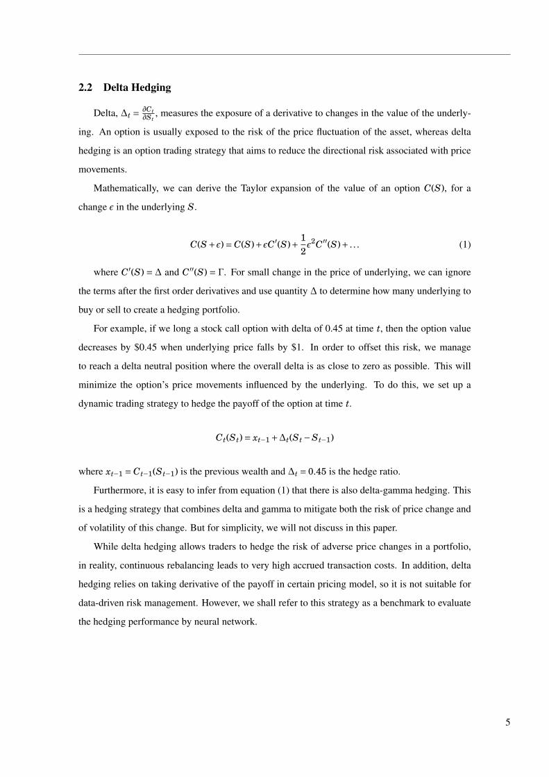
2.2 Delta Hedging
Delta, ∆t = ∂Ct∂St
, measures the exposure of a derivative to changes in the value of the underly-
ing. An option is usually exposed to the risk of the price fluctuation of the asset, whereas delta
hedging is an option trading strategy that aims to reduce the directional risk associated with price
movements.
Mathematically, we can derive the Taylor expansion of the value of an option C(S), for a
change ε in the underlying S.
C(S+ε)= C(S)+εC′(S)+ 12ε2C′′(S)+ . . . (1)
where C′(S) = ∆ and C′′(S) = Γ. For small change in the price of underlying, we can ignore
the terms after the first order derivatives and use quantity ∆ to determine how many underlying to
buy or sell to create a hedging portfolio.
For example, if we long a stock call option with delta of 0.45 at time t, then the option value
decreases by $0.45 when underlying price falls by $1. In order to offset this risk, we manage
to reach a delta neutral position where the overall delta is as close to zero as possible. This will
minimize the option’s price movements influenced by the underlying. To do this, we set up a
dynamic trading strategy to hedge the payoff of the option at time t.
Ct(St)= xt−1 +∆t(St −St−1)
where xt−1 = Ct−1(St−1) is the previous wealth and ∆t = 0.45 is the hedge ratio.
Furthermore, it is easy to infer from equation (1) that there is also delta-gamma hedging. This
is a hedging strategy that combines delta and gamma to mitigate both the risk of price change and
of volatility of this change. But for simplicity, we will not discuss in this paper.
While delta hedging allows traders to hedge the risk of adverse price changes in a portfolio,
in reality, continuous rebalancing leads to very high accrued transaction costs. In addition, delta
hedging relies on taking derivative of the payoff in certain pricing model, so it is not suitable for
data-driven risk management. However, we shall refer to this strategy as a benchmark to evaluate
the hedging performance by neural network.
5
2.3 Utility Function Method
2.3.1 Risk measure
In an idealized complete market, such as binomial model, with continuous-time trading, no
transaction costs, and unconstrained hedging, for any payoff X there exists a unique replication
strategy δ and a fair price p0 ∈ R such that p0 + (δ ·S)T − X = 0 holds P−a.s, where
(δ ·S)T :=T−1∑k=0
δk · (Sk+1 −Sk)
We denote by H u the unconstrained set of such trading strategies.
This strategy is the delta hedging we discuss above. In this paper, we assume a market without
trading coststhen the strategy should have the terminal wealth
PnLT (X , p0,δ) :=−X + p0 + (δ ·S)T
If δ and p0 do not have analytical results, we can work out the replication strategy by utility
function method.
First, we have to specify an optimality criterion which defines an acceptable “minimal price”
for any position. Such a minimal price is going to be the minimal amount of cash we need to add
to our position in order to implement the optimal hedge and such that the overall position becomes
acceptable in light of the various costs and constraints. We focus here on optimality under convex
risk measures as studied e.g. in Xu (2006) and Ilhan et al. (2008).
Definition 1 Assume that X , X1, X2 ∈ X represent asset positions. We call ρ : X → R a convex
risk measure if it has following properties:
1. Monotonicity: if X1 ≥ X2, then ρ (X1) ≤ ρ (X2). This implies that a portfolio with greater
future returns has less risk.
2. Convexity: ρ (αX1 + (1−α)X2) ≤ αρ (X1)+ (1−α)ρ (X2) for α ∈ [0,1]. This implies that a
merge of portfolios does not create extra risk.
3. Translation invariance: ρ(X+c)= ρ(X )−c for c ∈R. This implies that the addition of a sure
amount of cash reduces the risk by the same amount. In particular, when c = ρ(X ),ρ(X+c)=0, in other words, ρ(X ) is the least amount of capital that needs to be added to the position
X in order to make it acceptable in the sense that ρ(X + c)≤ 0.
6
2.3.2 Indifference price
Now, let ρ : X →R be such a convex risk measure and consider an optimization problem
π(X ) := infδ∈H
ρ (X + (δ ·S)T ) (2)
It is not difficult to conclude that π is also monotone decreasing and translation invariant, see
Buhler et al. (2018). We can then define an optimal replication strategy δ ∈H as a minimizer of
equation (2). Recalling the interpretation of Translation invariance, ρ(X ) as the minimal amount
of c that has to be added to the risky position X to make it acceptable for the risk measure ρ, this
also means that π(X ) is simply the minimal amount that the agent needs to charge in order to make
her terminal position acceptable, if she hedges optimally.
If we defined this as the minimal price, then we would exclude the possibility that having no
liabilities may actually have positive value. We then define the Indifference price p(X ) as the
amount of cash that a trader needs to charge in order to be indifferent between the position X and
making no trade at all(this indicates X = 0). Thus the indifference price would be the solution p to
π (−Z+ p)= π(0). By the Translation invariance property, we know that π (−Z+ p)= π (−Z)− p,
so the indifference price
p =π (−Z)−π (0) (3)
We can see that if there are no trading constraints and transaction costs, the indifference price
p coincides with the initial price of a replication portfolio if it exists and is unique (Buhler et al.
(2018)).
2.3.3 Exponential Utility Indifference Pricing
We define price q using exponential utility function U(x) :=−exp(−λx), x ∈ R with risk aver-
sion λ. From the discussion above, q should satisfy
supδ∈H
E [U (q− X + (δ ·S)T )]= supδ∈H
E [U ((δ ·S)T )]
exp(−λq)= supδ∈H E [U (−X + (δ ·S)T )]supδ∈H E [U ((δ ·S)T )]
q = 1λ
log(supδ∈H E [U (−X + (δ ·S)T ))]
supδ∈H E [U ((δ ·S)T )]
) (4)
In this case, if the trader charges q amount of cash, sells option with payoff X and trades in
7
the market according to δ, she then obtains the same expected utility as not selling the option.
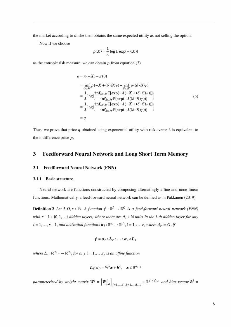
Now if we choose
ρ(X )= 1λ
logE[exp(−λX )]
as the entropic risk measure, we can obtain p from equation (3)
p =π (−X )−π (0)
= infδ∈H
ρ (−X + (δ ·S)T )− infδ∈H
ρ ((δ ·S)T )
= 1λ
log( infδ∈H E[exp(−λ (−X + (δ ·S)T ))]
infδ∈H E[exp(−λ((δ ·S)T ))]
)= 1λ
log( infδ∈H E[exp(−λ (−X + (δ ·S)T ))]
infδ∈H E[exp(−λ((δ ·S)T ))]
)= q
(5)
Thus, we prove that price q obtained using exponential utility with risk averse λ is equivalent to
the indifference price p.
3 Feedforward Neural Network and Long Short Term Memory
3.1 Feedforward Neural Network (FNN)
3.1.1 Basic structure
Neural network are functions constructed by composing alternatingly affine and none-linear
functions. Mathematically, a feed-forward neural network can be defined as in Pakkanen (2019)
Definition 2 Let I,O, r ∈ N. A function f : RI → RO is a feed-forward neural network (FNN)
with r−1 ∈ 0,1, . . . hidden layers, where there are di ∈N units in the i-th hidden layer for any
i = 1, . . . , r−1, and activation functions σi : Rdi →Rdi , i = 1, . . . , r, where dr :=O, if
f =σr Lr · · · σ1 L1
where L i : Rdi−1 →Rdi , for any i = 1, . . . , r, is an affine function
L i(x) :=W ix+bi, x ∈Rdi−1
parameterised by weight matrix W i =[W i
j,k
]j=1,...,di ,k=1,...,di−1
∈ Rdi×di−1 and bias vector bi =
8
(bi
1, . . . ,bidi
)∈Rdi , with d0 := I. We shall denote the class of such functions f by
Nr (I,d1, . . . ,dr−1,O;σ1, . . . ,σr)
We call r,d1, . . . ,dr−1 the hyperparameters of the FNN and the weights and biases in θ =(W1, . . . ,W r, b1, . . . ,br) parameters of the network, together with the activation functionsσ1, . . . ,σr,
they determine the architecture of the network.
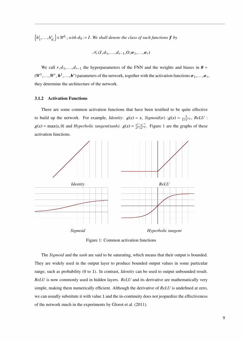
3.1.2 Activation Functions
There are some common activation functions that have been testified to be quite effective
to build up the network. For example, Identity: g(x) = x, Sigmoid(σ) :g(x) = 11+e−x , ReLU :
g(x) = maxx,0 and Hyperbolic tangent(tanh): g(x) = ex−e−x
ex+e−x . Figure 1 are the graphs of these
activation functions.
Identity
Sigmoid
ReLU
Hyperbolic tangent
Figure 1: Common activation functions
The Sigmoid and the tanh are said to be saturating, which means that their output is bounded.
They are widely used in the output layer to produce bounded output values in some particular
range, such as probability (0 to 1). In contrast, Identity can be used to output unbounded result.
ReLU is now commonly used in hidden layers. ReLU and its derivative are mathematically very
simple, making them numerically efficient. Although the derivative of ReLU is undefined at zero,
we can usually substitute it with value 1 and the in-continuity does not jeopardize the effectiveness
of the network much in the experiments by Glorot et al. (2011).
9
3.1.3 Loss Functions
The notions of task and optimality are characterised by a loss function.
` : RO ×RO →R
Given input x ∈ RI and reference value y ∈ RO we compute the realised loss as `(f (x), y). In
theory, if x and y are a random vector (X ,Y ) from a known distribution, we could try to seek
optimal f by minimising the risk
E[`(f (X ),Y )]
However, in practice, this distribution is usually unknown. Hence, we resort to empirical methods
with samples x1, . . . , xN of x and y1, . . . , yN of y for some large N ∈ N. For the sake of SGD,
we also consider averaging over any subset, minibatch, B ⊂ 1, . . . , N of samples. Notice that
once the architecture and the activation functions have been fixed, the network fθ = f is then fully
determined by the parameter vector θ we need to optimize. So, we calculate
LB(θ) := 1#B
∑i∈B
`(fθ
(xi
), yi
)
as the minibatch empirical risk, where #B is the number of elements in set B.
In this paper we use two types of loss function: squared loss and exponential utility function.
3.1.4 SGD and Backpropagation
Stochastic gradient descent(SGD) is a gradient descent method using over different mini-
batches. Consider first minimizing a differentiable objective function F : Rd → R over x(t) ∈Rd, t > 0, the gradient descent method achieve the optimal solution by an iterative algorithm
x(t+η)= x(t)−η∇F(x(t))
given initial x(0), where
−∇F = x(t+η)− x(t)η
where η is the step size or learning rate. Under certain assumptions on F, which guarantee the
existence of a unique minimizer and are stronger than mere convexity, it is shown in Schmidhuber
(2015) that x(t) tends to the minimizer as t →∞.
While this method seems to be trivial to implement, in practice, it is computationally costly
10
to directly minimize the risk with large N. Not to mention that gradient descent may also lead
to overfitting. To this end, we apply the SGD to the training of network as in Pakkanen (2019).
Firstly, we randomly split the training data into k minibatches: B1, . . . ,Bk ⊂ 1, . . . , N, and each
minibatch contains m samples, so that N = km and⋃k
i=1 Bi = 1, . . . , N. Then the parameter
vector θ is updated by
θi := θi−1 −η∇θLBi (θi−1) , i = 1, . . . ,k
with initial θ set in advance. After that, we regard one round of training through all the minibatch
as an epoch. This algorithm is then repeated over multiple epochs, each round with newly spilt
minibatches, while initialising θ with the last value of the previous epoch.
If the learning rate ηwere set and fixed at a rather high value in the beginning, the route of SGD
might overshoot or zigzag, whereas low η could also lead to very slow convergence otherwise. To
tackle this issue, several refinements of SGD have been proposed, to adaptively tune η or to seek
update gradient directions better than ∇θL . Some well-known refinements of SGD include the
Nesterov momentum method by Nesterov (1983) and Ilya Sutskever and Hinton (2013), RMSProp
by Tieleman and Hinton (2012) and Adam by Kingma and Ba (2014), the last of which is perhaps
the most renowned optimisation method in deep learning at the moment. In Adam, the parameter
update direction of ∇θL is determined by an exponentially weighted moving average (EWMA)
of previous gradients, while the learning rate η is adjusted using an EWMA of squares of previous
gradients.
To compute the gradient of the empirical risk ∇θLB(θ), we apply a special case of algorithmic
differentiation - backpropagation. This algorithm provides a way to efficiently compute the exact
value of the gradient in feedforward neural network, but for chosen θ only. Here, we only highlight
the main ideas and results as in Higham and Higham (2019) and skip the proof and calculation.
In short, backpropagation is based on chain rule. The minibatch enpirical risk, by linearity, can be
written as
∇θLB(θ)= 1#B
∑i∈B
∇`(fθ
(xi
), yi
)So our aim is to work out the expressions of loss function’s derivatives with respect to all the
weights and biases. We now introduce some notations for presenting the results. For x ∈RI ,
zi =(zi
1, . . . , zidi
):= L i
(ai−1
)=W iai−1 +bi, i = 1, . . . , r
ai =(ai
1, . . . ,aidi
):= g i
(zi
), i = 1, . . . , r,
a0 := x
11
so that fθ(x) = ar and ` (fθ(x), y) = ` (ar, y). In addition, we introduce a term called adjoint
δi =(δi
1, . . . ,δidi
)∈Rdi by
δij := ∂`
∂zij
, j = 1, . . . ,di
for any i = 1, . . . , r. Using the chain rule, we can derive all the derivatives by a backward recursive
where ¯ stands for the component-wise Hadamard product of vectors. In this way, we can estimate
the derivatives of empirical risk and update the parameter θ in the SGD.
3.2 Long Short Term Memory (LSTM)
Recurrent neural networks(RNN) are based on David Rumelhart’s work in 1986, and are now
widely used in translation, speech recognition, image processing and other areas. What differen-
tiates RNN from FNN is that the output of RNN is subsequently fed back to the network, which
makes RNN a little more complicated than FNN. It is more straightforward to understand the
structure when we unfold the RNN to FNNs.
Figure 2: Recurrent neural network
We can see from Figure 2 that the loop in the structure of RNN ensures information to pass on
on. When unfolding RNN, it can be thought of multiple copies of the same network, each passing
a message from one step of the network to the next. So each round of training remembers the
12
information in previous training, and this network is particular suitable for predicting something
that is path dependent.
However, RNN also has its drawbacks. Gradient vanishing and exploding are very likely
to occur during the backpropagation, making RNN unable to learn to connect the information(
Nielsen (2015)). This issue is due to the fact that, unfolding RNN with N time steps is a very deep
feedforward network that duplicates N times, and in backpropagation the gradient in early layers
is the product of terms from all the later layers. When there are many layers, the gradient tends
to be unstable and may eventually explode or vanish. Also, because the product that gives the
gradient contains many instances of the same weight, the product goes either exponentially small
or exponentially big. In other words, the fact that the unrolled RNN is composed of duplicates of
the same network makes the unrolled network’s "unstable gradient problem" more severe than in
a normal deep feedforward network.
Having said that, long short term memory network(LSTM) - a special kind of RNN developed
by Hochreiter and Schmidhuber (1997) - is able to tackle the vanishing and exploding gradient
problem discussed above, that is, is capable of learning long-term dependencies. Currently, LSTM
is perhaps the most famous and popular RNN and it works tremendously well on a large variety
of problems. We would now give a brief introduction of it.
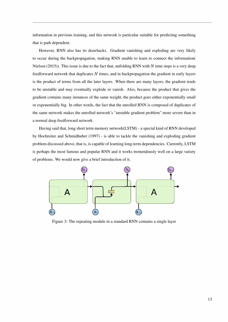
Figure 3: The repeating module in a standard RNN contains a single layer
13
Figure 4: The repeating module in an LSTM contains four interacting layers
Figure 3 and Figure 4 give the structures of RNN and LSTM respectively, where xt represents
input and ht stands for output. The key insight of LSTM is that we create a cell state Ct (upper
horizontal line in Figure 4) - a conveyor belt that stores and updates history information and then
pass it to the next step, with only some minor linear interactions. To make sure we preserve and
pass the information appropriately, we introduce three gates into LSTM layer. These three gates
are composite functions with the form of a ordinary layer f (x)=σ(Wx+b), where σ(·) is Sigmoid
activation function, W a weight matrix and b bias vector. Now we explain the details of these three
gates and how they function in a simple LSTM layer.
• Forget gate layer f t looks at ht−1 and xt, and decides what information we should leave
aside when entering into Ct.
f t =σ(Wf · [ht−1, xt]+b f
)In some cases, we want to forget useless properties of old subject.
• Input gate layer i t also looks at ht−1 and xt, and decides what new values we should store
into Ct.
i t =σ (Wi · [ht−1, xt]+bi)
Here, a tanh layer creates this new values as a vector Ct
Ct = tanh(WC · [ht−1, xt]+bC)
With the forget gate and the input gate, we then update the cell state Ct−1 into Ct by com-
14
bining the old and new information
Ct = f t ∗Ct−1 + i t ∗ Ct
• Output gate ot again looks at ht−1 and xt,
ot =σ (Wo [ht−1, xt]+bo)
and decides what information we should pass on from cell state Ct to the output ht
ht = ot ∗ tanh(Ct)
4 Deep Hedging
Having the introduction of hedging and neural network showing above, we can now present
the framework of deep hedging.
4.1 Model setting
First, we set up the FNN model and begin with a simple test on European call option where
we can easily compare the deep hedging strategy with Black Scholes delta hedging approach.
Deep hedging works in discrete time, so we divide interval [0,1] into T subintervals with grid
points tn = nT ,n = 0,1,2, . . . ,T and interval h = 1
T .
Our aim is to use feedforward neural network to develop a self-financing trading strategy to
hedge the payoff (ST − K)+. Such a strategy is specified by its initial wealth x0 and position
γt in the underlying stock at time t for any t = 0,1, . . . ,T. Assuming zero interest rate and zero
transaction cost, by the self-financing property, the terminal wealth of the strategy can be expressed
as
VT = x0 +T∑
t=1γt−1 (St −St−1)
Now with x0 and price path St fixed, we aim to match the VT to the payoff (ST −K)+, that is, train
neutal network whose output is γt so that the
PnL=VT − (ST −K)+
= x+T∑
t=1γt−1 (St −St−1)−
(S0 +
T∑t=1
(St −St−1)−K
)+ (6)
15
approaches 0 as close as possible.
By adaptedness, γt must be a function of the past prices St,St−1, . . . ,S0 only. We represent
trading strategy γ as a neural network, whose inputs are the available market data and output is the
hedging position
γt = f t (St,St−1, . . . ,S0)
where f t is a neural network for any t = 0,1, . . . ,T −1. In fact, since S is a Markov process, we
can rewrite γ as a simpler neural network f : [0,1]×R→R so that
r t = f(
tT
,St
), t = 0,1, . . . ,T −1
Finally, we specify a feedforward neural network in Keras as follow
f ∈N4(2,100,100,100,1;ReLU ,ReLU ,ReLU ,Sigmoid)
where we choose Sigmoid as the output activation function due to the financial intuition that the
hedging position should be between 0 and 1. We adapt both squared loss and exponential utility
function as its loss function, since the later one can achieve hedging and pricing at the same time.
During the training of FNN, we set epochs= 5,batch size= 10 and choose Adam as the optimizer.
For LSTM, we specify a model containing one LSTM layer with 10 units and a output layer
with Sigmoid function. However, we observe that if we use the same training procedure as in FNN
to train the LSTM, the network converges quite slowly. To accelerate the speed of convergence, we
separate the training of LSTM into two rounds. In the first round, we set epochs = 5,batch size =50, and Adam as the optimisation method with a relatively large initial leaning rate = 0.01. Then
in the second round, we change the learning rate into 0.001 and others remain the same.
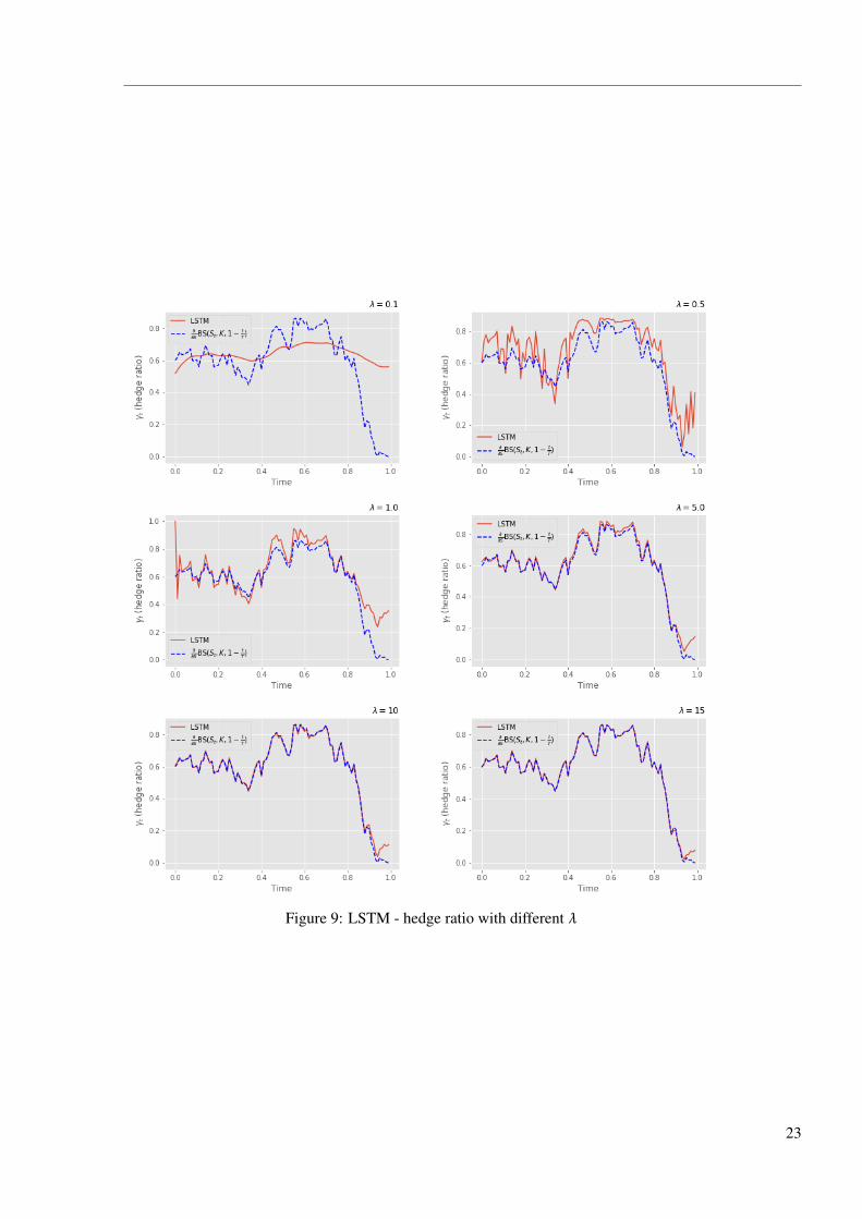
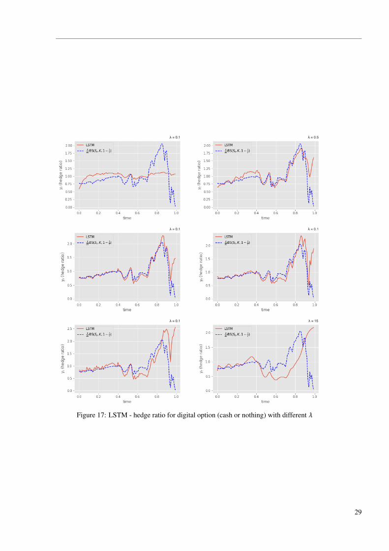
For large T the price process St is close to the continuous Black Scholes price process, thus
the hedging ratio γt should in theory be close to the Black Scholes delta hedging position
γBSt = ∂
∂SC
(St,K ,1− t
T
)
which amounts to perfect replication, PnL= 0.
4.2 Advantages and Drawbacks
Compared to delta hedging, deep hedging is in principle model-free and data-driven. The real
data in the market are very likely insufficient for training the network, however, in practice, we
16
require a market simulator to generate the data we need. One of the common ways to tackle this
is model calibration. We first need to set up a dynamic model for the price of underlying and
calibrate it using market data. For instance, we intend to calibrate the Heston model with the price
process satisfying
dSt =µStdt+pvtStdWS
t
in which the volatility vt is a CIR process
dvt = κ (θ−vt)dt+ξpvtdWvt
where µ is drift, θ > 0 is long term mean, κ> 0 is mean reversion and WSt and Wv
t are two standard
Brownian motions with correlation ρ. First, we use quote data of call and put option in the market
to determine µ,θ, κ and ρ. Then, we simulate enough price paths and train the network. Finally,
we use this network to test real data.
Another strength of deep hedging is that various market imperfections, such as trading cost,
are relatively straightforward to incorporate to the framework, while in analytical method they are
uaually very hard to dealt with.
5 Experiment
5.1 Data generation
We generate a price path St by first generating T independent N(0,1) variables W1,W2, . . . ,WT
and computing
St+1 = St +µhSt +σp
hStWt+1
where µ is drift and σ is volatility. We use St to approximate the price in continuous Black Scholes
model.
In the experiment, we simulate N = 100,000 price paths and set the original parameters
µ= 0.0,σ= 0.5,T = 100,S0 = 1
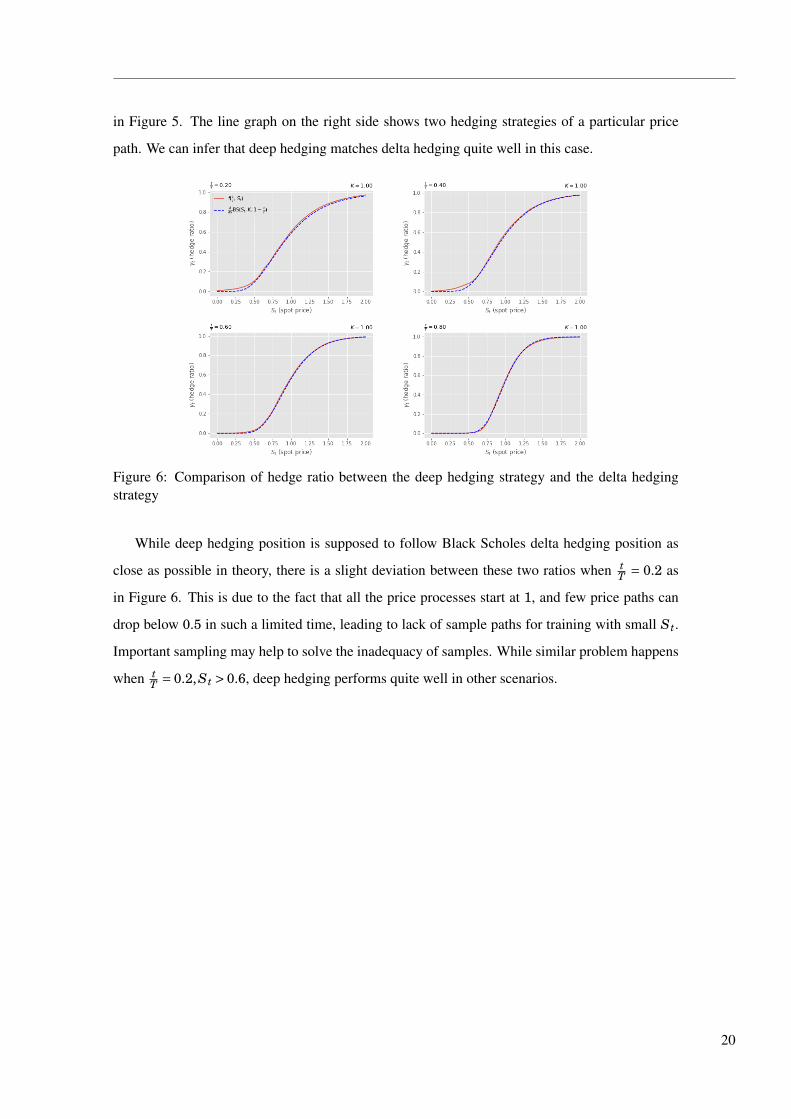
5.2 Result
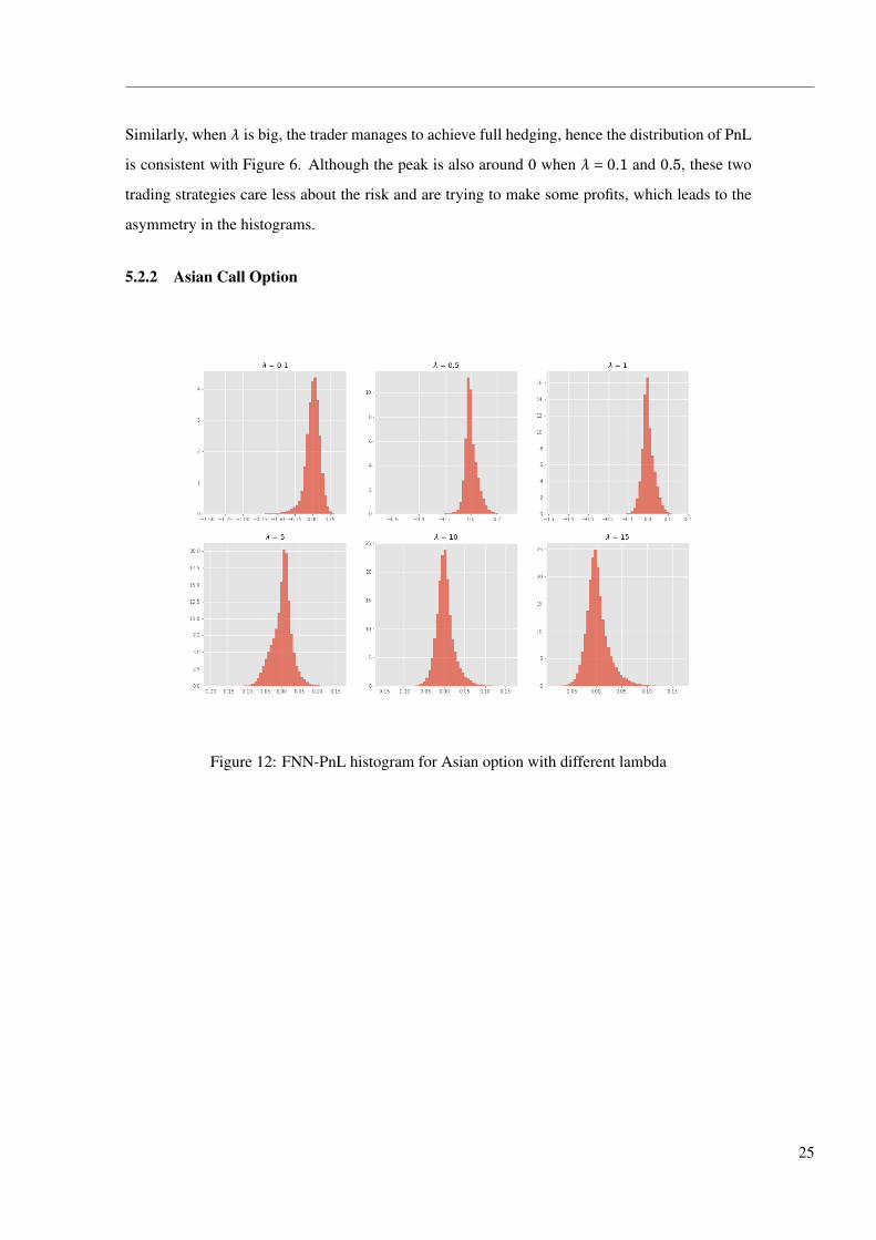
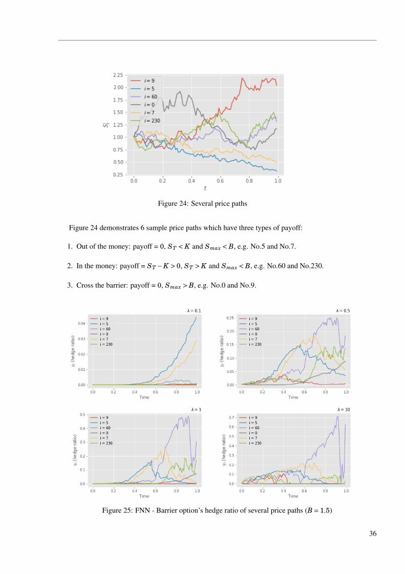
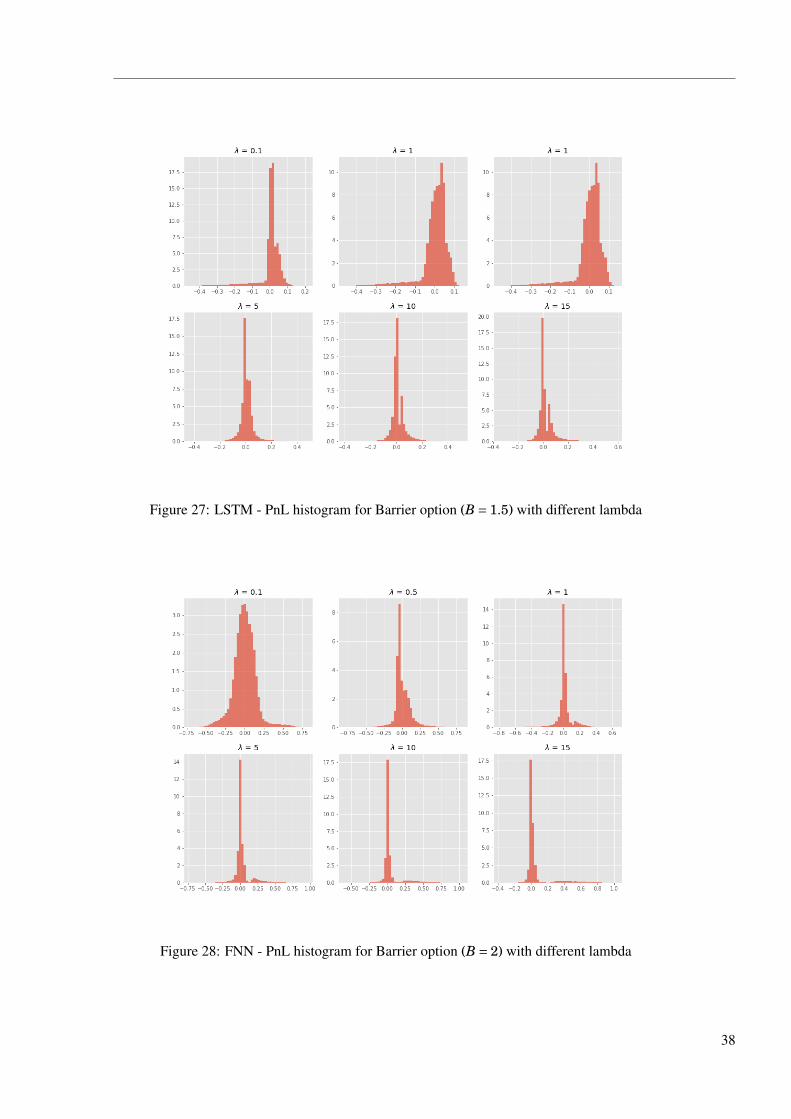
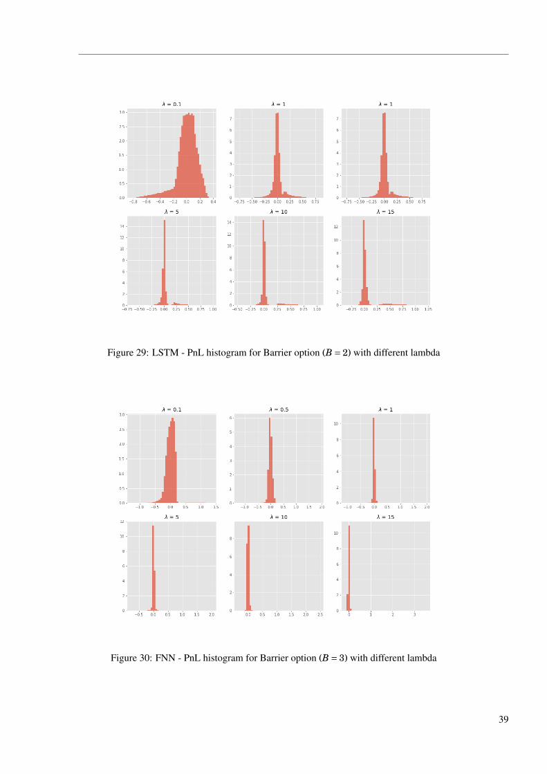
We examine deep hedging on five types of options: European call option, Asian call option,
digital option(cash or nothing), digital option(asset or nothing) and barrier option(up and out). Part
17
of results can be seen from the tables below.
Table 1: Indifference price of different option using FNN and LSTM model
Analytical /MC price λ = 0.1 λ = 0.5 λ = 1
FNN LSTM FNN LSTM FNN LSTM
European calll option 0.1974 0.1973 0.1977 0.1976 0.1978 0.1976 0.1978
Asian call option 0.1131 0.1141 0.1139 0.1143 0.1136 0.1144 0.1138
Digital option (cash or nothing) 0.4013 0.4040 0.4051 0.4082 0.4107 0.4116 0.4160
Digital option (asset or nothing) 0.5987 0.6004 0.6030 0.6041 0.6106 0.6079 0.6191