20 Pricing in Supply Chain under Vendor Managed Inventory Subramanian Nachiappan 1 and Natarajan Jawahar 2 1,2 Department of Mechanical Engg., Thiagarajar College of Engineering Madurai 1 Nottingham University Business School, Jubilee Campus, Nottingham 1. Introduction The successful implementation of supply chain management depends on many soft issues (strategic/behavioural) such as organizational resistance to change, inter-functional conflicts, joint production planning, profit sharing, team oriented performance measures, channel power shift, information sharing, real time communication, inventory and technical compatibility (Min & Zhou 2002). Many of the above issues in SCM are conceptually addressed and lot of scope exists for improving the performance of SC with good modelling. The soft issues of supply chain models can be dealt through proper information sharing, communication and coordination between the stages of supply chain. Vendor managed inventory (VMI) is a proven concept for successful collaborative and cooperative agreements in supply chain. While research has been slowly increasing in the area of vendor managed inventory, it has received very little attention in current operations literature. This chapter focuses on the soft issues of profit sharing and pricing under vendor managed inventory systems. Two vital parameters that govern the operation of a supply chain are: sales price at buyers market, and contract price between vendor and buyer. Sales price is significant in the sense that it determines the overall profit of the supply chain, referred here as channel profit. This chapter proposes five mathematical models under VMI environment for determination of optimal sales quantity for each buyer which maximizes the channel profit and subsequently to derive the sales and contract price from the optimal sales quantity. 2. Two-echelon supply chains In the present internet / E-commerce arena, the stages in SC are less and the manufacturers access the customer requirement through retailers. Dell computers have reoriented its strategy by reducing it’s down-stream stages and sells through its retail outlets in a particular region (Chopra, 2003). Procter and Gamble manages, monitors and replenishes its FMCG products in Wal-Mart stores (Clark & Croson, 1994). The success stories of these Giants have led the researchers to concentrate on two-echelon supply chain (Cachon & Zipkin, 1999). The two-echelon can be considered sequentially between any two of these stages such as suppliers, manufacturers, distributors, wholesalers, retailers, and end- customer. There are three types of environments addressed in two-echelon SC and they are: Source: Supply Chain,Theory and Applications, Book edited by: Vedran Kordic, ISBN 978-3-902613-22-6, pp. 558, February 2008, I-Tech Education and Publishing, Vienna, Austria Open Access Database www.intehweb.com www.intechopen.com
Transcript
20
Pricing in Supply Chain under Vendor Managed Inventory
Subramanian Nachiappan1 and Natarajan Jawahar2
1,2Department of Mechanical Engg., Thiagarajar College of Engineering Madurai 1Nottingham University Business School, Jubilee Campus, Nottingham
1. Introduction
The successful implementation of supply chain management depends on many soft issues (strategic/behavioural) such as organizational resistance to change, inter-functional conflicts, joint production planning, profit sharing, team oriented performance measures, channel power shift, information sharing, real time communication, inventory and technical compatibility (Min & Zhou 2002). Many of the above issues in SCM are conceptually addressed and lot of scope exists for improving the performance of SC with good modelling. The soft issues of supply chain models can be dealt through proper information sharing, communication and coordination between the stages of supply chain. Vendor managed inventory (VMI) is a proven concept for successful collaborative and cooperative agreements in supply chain. While research has been slowly increasing in the area of vendor managed inventory, it has received very little attention in current operations literature. This chapter focuses on the soft issues of profit sharing and pricing under vendor managed inventory systems. Two vital parameters that govern the operation of a supply chain are: sales price at buyers market, and contract price between vendor and buyer. Sales price is significant in the sense that it determines the overall profit of the supply chain, referred here as channel profit. This chapter proposes five mathematical models under VMI environment for determination of optimal sales quantity for each buyer which maximizes the channel profit and subsequently to derive the sales and contract price from the optimal sales quantity.
2. Two-echelon supply chains
In the present internet / E-commerce arena, the stages in SC are less and the manufacturers access the customer requirement through retailers. Dell computers have reoriented its strategy by reducing it’s down-stream stages and sells through its retail outlets in a particular region (Chopra, 2003). Procter and Gamble manages, monitors and replenishes its FMCG products in Wal-Mart stores (Clark & Croson, 1994). The success stories of these Giants have led the researchers to concentrate on two-echelon supply chain (Cachon & Zipkin, 1999). The two-echelon can be considered sequentially between any two of these stages such as suppliers, manufacturers, distributors, wholesalers, retailers, and end-customer. There are three types of environments addressed in two-echelon SC and they are: Source: Supply Chain,Theory and Applications, Book edited by: Vedran Kordic, ISBN 978-3-902613-22-6, pp. 558, February 2008, I-Tech Education and Publishing, Vienna, Austria
Ope
n A
cces
s D
atab
ase
ww
w.in
tehw
eb.c
om
www.intechopen.com
Supply Chain: Theory and Applications
388
i. Single vendor-single buyer (Banerjee, 1986; Goyal, 1997; Hill, 1997; Viswanathan, 1998; Bhattacharjee & Ramesh, 2000; Goyal & Nebebe, 2000; Hoque & Goyal, 2000; Dong & Xu, 2002; Lee & Chu, 2005),
ii. Single vendor-multiple buyers (Lu 1995; Gavirneni, 2001 and Yao & Chiou 2004) and iii. Multiple vendors - multiple buyers (Cachon, 2001; Minner 2003; Sedarage et al., 1999;
Ganeshan, 1999). The above three environments addressed by the numerous researchers were operating under independent mode with various objectives. Single vendor-single buyer is considered as an idealistic one in dealing with bottleneck cases and the remaining two cases represent the most practical situations. This chapter proposes five types of environments in two-echelon supply chain model operating under vendor managed inventory mode as given below (Nachiappan et al. 2006; Nachiappan & Jawahar 2007; Nachiappan et al. 2007; Nachiappan et al. 2007a). The parameters involved are explained at the end of the model description. i. Single Vendor Single Buyer (SV_SB) The single vendor single buyer as shown in figure1 is known as an idealistic case.
Figure 1 SV_SB Model
ii. Single Vendor Multiple Buyer’s (SV_MB) Single vendor multiple buyer’s case is shown in figure 2. Few examples for this case cases are: Tamilnadu Cooperative milk producer’s federation limited (AAVIN) Madurai, India (Single Vendor) selling its milk products to 423 commission agents (Multiple Buyers) in and around Madurai; Bharat Petroleum Corporation, Cochin, India (Single Vendor) distributing its petroleum products to 2500 sales points (Multiple Buyers) in southern part of India. iii. Single Vendor Multiple Buyer’s with Outsourcing (SV_MBO) When the cumulative demand of all buyers goes up more than the vendor capacity, outsourcing is the option for the vendor to satisfy buyer’s demand. Nowadays outsourcing is becoming part of regular activity in both manufacturing organizations and service providers. Globalization pushes both of them into highly competitive environment. Outsourcing occurs because a firm may find it less profitable or not feasible to produce all required capabilities in-house. Outsourcing is an acceptable strategy to meet the excess demands than the limited capacity of the vendor. Outsourcing incorporated with SV_MB model, operating under VMI mode as shown in figure 3 is referred as Single Vendor Multiple Buyers with Outsourcing (SV_MBO)
a1
Vendor
Buyer Wi P(y1)
b
y1
Demand Functions
www.intechopen.com
Pricing in Supply Chain under Vendor Managed Inventory
389
Figure 2. SV_MB model
Figure 3. SV_MBO Model
Demand Function
Vendor
Buyer1 P(y1)
Buyer2 P(y2)
***
Buyerj P(yj)
***
Buyer n P(yn)
P(y1)
a1
y1
b1
P(y1)
a2
y2
b2
P(yj)
aj
yj
bj
P(yn)
an
yn
bn
W1
W2
Wj
Wn
Demand Function
Vendor
Buyer1 P(y1)
Buyer2 P(y2)
***
Buyerj P(yj)
***
Buyer n P(yn)
P(y1)
a1
y1
b1
P(y1)
a2
y2
b2
P(yj)
aj
yj
bj
P(yn)
an
yn
bn
W1
W2
Wj
Wn
Vendor for outsourcing
Outsourcing Quantity ‘Oy’
Outsourcing Cost ‘Oc’
www.intechopen.com
Supply Chain: Theory and Applications
390
iv. Multiple Vendors Multiple Buyers (MV_MB) Few examples of multiple vendors multiple buyers as shown in figure 4 are as follows: Gold suppliers (Multiple Vendors) are selling gold through thousands of retailer’s network (Multiple Buyers) and numerous grain suppliers (Multiple Vendors) supplying grains through thousands of retailers (Multiple Buyers).
Figure 4. MV_MB model
v. Multiple Vendors Multiple Buyers with Outsourcing (MV_MBO) Similar to SV_MBO whenever the cumulative demand of all buyers exceeds the capacity of all vendors, outsourcing is the only option for the vendors to satisfy the buyers demand. The MV_MB model with outsourcing (MV_MBO) is shown in figure 5. Model Parameters The demand pattern, sales quantity range at the buyers end and the importance of contract price between vendor(s) and buyer(s) are given below Demand Pattern: The sales quantity of any product at a particular location is greatly influenced by its sales price‘P(yj)’ (Waller et. al., 2001). It depends on the factors such as necessity of the commodity (essential or occasional), purchasing power of the customers and nature of the product (perishable or storable). The general observation is that the higher sales price results low sales quantity and vice versa, provided the reputation and history of the company or brand value have no greater impact on the customers and/or there is at least one stiff customer (local or global) to control the sales price.
W11, x11
W21, x21
Vendor 1 Buyer1 P(y1)
Buyer2 P(y2)
Buyerj P(yj)
***
Buyer n P(yn)
P(y1)
a1
y1
b1
P(y1)
a2
y2
b2
P(yj)
aj
yj
bj
P(yn)
an
yn
bn Wmn, xmn
Vendor 2
i
----
Vendor m
Wij, xij
Demand Function
www.intechopen.com
Pricing in Supply Chain under Vendor Managed Inventory
391
Figure 5. MV_MBO model
Figure 6. Relationship between sales price and sales quantity
W11, x11
W21, x21
Vendor 1 Buyer1 P(y1)
Buyer2 P(y2)
Buyerj P(yj)
***
Buyer n P(yn)
P(y1)
a1
y1
b1
P(y1)
a2
y2
b2
P(yj)
aj
yj
bj
P(yn)
an
yn
bn Wmn, xmn
Vendor 2
i
----
Vendor m
Wij, xij
Vendor for outsourcing
Demand Function
yj
yjmin yjmax
∆yj
∆P(yj)aj
bj = ∆P(yj) ∆yj
P(yj)
www.intechopen.com
Supply Chain: Theory and Applications
392
Taking into account the above for consideration, the relationship between ‘P(yj)’ and ‘yj’ may be assumed to behave linearly (Lau & Lau, 2003) and is given as:
P(yj) = aj – bjyj (1)
Where, aj and bj are the intercept of ‘P(yj)' axis and the slope of sales quantity /curve respectively in the sales price vs sales quantity graph shown in figure 6. This becomes the demand function for the buyer Sales Quantity Range: Sales quantity lies between a specific range between yjmin and yjmax and the validity of the assumption of linear demand function holds very well within this range. Contract Price: Contract Price (wij) is a price mutually agreed between ith vendor and jth buyer which decide the profits of both vendor and buyer and hence it is considered as vital. Usually it lies between sales price and cost of manufacturing. Nature of the product, demand and logistic cost play critically in the fixation of contract price. The commodities that have good reputation and high demand are usually fast moving and involve low risk (probability of loss). In these circumstances, the buyer accepts the contract price closer to sales price, even with meager margin on the reasons stated as: Loss due to obsolescence is negligible; Non availability of the commodity results in loss of customers that would definitely reduce the overall turnover of the outlet; Storage/Holding cost is normally low. However in an another scenario, where the product is new and demand is not yet stabilized, the contract price is expected to settle at a lower level, closer to cost of production. The possible reasons are: Outlets of the commodity take the task of promoting the new product; Cost of inventory is expected to be high. In such cases, ethical issues like cooperation, revenue and knowledge sharing are needed to compete with the existing commodity and consolidate its market. The above discussions point out that contract price is a variable, which is dependent on location, competitiveness of the products and production and operational costs between vendor and buyer. This shows that contract price play a vital role in the context of revenue sharing.
3. Vendor managed inventory
The soft issues of SC models can be dealt through proper information sharing, communication and coordination between the stages of SC. Examples of collaborative and cooperative agreements come in many forms and by many names, including Continuous Replenishment (CR), Vendor Managed Inventory (VMI), Collaborative Forecasting, Planning and Replenishment (CFPR) and Information Sharing Programs (ISP). The overall goal shared by all these programs is to reduce costs and to increase efficiency in the SC by sharing the information and/or by the transfer of decision rights (Mishra & Raghunathan, 2004; Fry, 2002; Ballou et al., 2000; Hammond, 1990). VMI is a proven concept for successful collaborative and cooperative agreements in SC. The core concept of VMI has been that the supplier monitors the customers’ demand and inventory and replenishes that inventory as needed with no action on the part of the customer (Dong & Xu, 2002 ; Disney & Towill, 2002). Waller et al. (2001) noted that the main advantages of VMI were reduced costs and increased customer service levels to one or both of the participating members. VMI, however, has received very little attention in current operations’ literature, particularly operations texts, but it has been widely recognized by industry leaders, such as Wal-Mart and the Campbell soup company for creating a competitive advantage. Franchise organizations have also made use of VMI to provide a higher level of operating efficiency
www.intechopen.com
Pricing in Supply Chain under Vendor Managed Inventory
393
(Williams, 2000). Cetinkaya & Lee (2000) noted that, with VMI, inventory carrying costs were generally reduced, as were stock out problems while the approach offered the ability to synchronise inventory and transportation decisions. VMI has differed from a fixed-order interval model or a fixed-order quantity model in that neither the time nor the quantity of replenishment was necessarily fixed. The supplier was responsible for managing the inventory at the customer’s location, generally using information technology, and for sending the correct amount at the correct time (Burke, 1996; Parks & Popolillo, 1999). While research has been slowly increasing in the area of VMI, certain segments of business have appeared to be getting less attention than others (Latamore & Benton, 1999). The SC’s of large retail and manufacturing organizations have been the foci of most of the research. Mabert & Venkataramanan (1998) pointed out that little work had been carried out in applying SCM techniques to service sectors. Therefore this chapter concentrates on VMI systems for two-echelon models in the service sectors.
3.1 Mathematical representation of vendor operations and costs
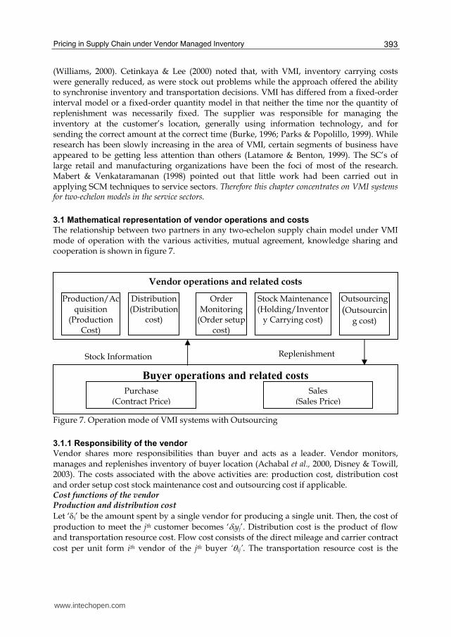
The relationship between two partners in any two-echelon supply chain model under VMI mode of operation with the various activities, mutual agreement, knowledge sharing and cooperation is shown in figure 7.
Figure 7. Operation mode of VMI systems with Outsourcing
3.1.1 Responsibility of the vendor
Vendor shares more responsibilities than buyer and acts as a leader. Vendor monitors, manages and replenishes inventory of buyer location (Achabal et al., 2000, Disney & Towill, 2003). The costs associated with the above activities are: production cost, distribution cost and order setup cost stock maintenance cost and outsourcing cost if applicable. Cost functions of the vendor Production and distribution cost
Let ‘δi’ be the amount spent by a single vendor for producing a single unit. Then, the cost of
production to meet the jth customer becomes ‘δiyj’. Distribution cost is the product of flow and transportation resource cost. Flow cost consists of the direct mileage and carrier contract
cost per unit form ith vendor of the jth buyer ‘θij’. The transportation resource cost is the
Stock Information Replenishment
Buyer operations and related costs
Sales
(Sales Price)Purchase
(Contract Price)
Vendor operations and related costs
Production/Acquisition
(Production Cost)
Distribution(Distribution
cost)
Order Monitoring
(Order setup cost)
Stock Maintenance(Holding/Inventor
y Carrying cost)
Outsourcing (Outsourcin
g cost)
www.intechopen.com
Supply Chain: Theory and Applications
394
indirect cost such as the mode of transport, human router cost and administrative costs and
termed as ‘γij’ per unit demand for the jth buyer from ith vendor (Dong and Xu, 2002).
Therefore, the distribution cost = (θijyij)(γijyij). The distribution cost varies parabolically depending upon the increase in quantity and mode of transportation. Since in VMI mode, the vendor has to monitor inventory and to replenish products as and when required, there will be exponential variation in distribution cost depending upon the increase in quantity and mode of transportation.
PDij =δi yj + γijθij yj2 (2)
Order and stock maintenance cost The vendor monitors the stock status and replenishes the stock. The buyer does not initiate orders. Therefore the order / setup cost per replenishment ‘SijVMI’ associated with continuously monitoring the stock status is assumed to be the sum of order/setup cost of the vendor ‘SSi’ and the order/setup cost of the buyer ‘Sbj’ (Dong & Xu, 2002). Therefore cost involved to replenish the batches ‘Qij’ of demand of the jth buyer ‘yj’ is given as Order / setup cost for replenishment = ((SSi + Sbj)yj/Qij). Inventory, whatever is the mode of operation, is held at both vendor and buyer locations HSi and Hbj are the cost of holding one unit per unit time at the ith vendor and the jth buyer’s location respectively. In order to replenish Qij to buyer ‘j’ the vendor ‘i’ accumulates this before delivery. Therefore the vendor ‘i’ holds an average inventory of Qij/2 to replenish buyer ‘j’ and VMI cost of holding inventory (HijVMI) becomes the sum of HSi and Hbj (Dong & Xu, 2002). Therefore the stock maintenance cost is given as (HSi+Hbj) Qij/2. Thus the order and stock maintenance cost OSMij of the vendor is the sum of the order setup cost and the average inventory holding cost and is as follows:
OSMij = (SSi + Sbj)yj/Qij + (HSi+Hbj) Qij/2 (3)
In this mode of operation the replenishment process takes place instantaneously, therefore to minimize the OSMij, Economic Order Quantity (EOQij) for buyer is determined by equating the first differential of OSMij to zero.
d(OSMij)/dQj = 0
EOQ ij = [2(SSi+Sbj)yj / (HSi+Hbj)] 1/2 (4)
Substituting EOQj for Qj, in equation (3)
OSMij =[2(HSi+Hbj)(SSi+Sbj)yj]1/2 (5)
Outsourcing cost:
Whenever, the aggregate sales quantity ( yj
n
j
∑=1
) of all the buyers exceeds the capacity ‘C’
of the vendor, then the vendor has to outsource the extra quantities ‘oy’ ( = yj
n
j
∑=1
-C). It is
assumed that an additional cost incurred for vendor to outsource a unit is ‘┟’ times of unit
production cost ‘δ’. There fore outsourcing
www.intechopen.com
Pricing in Supply Chain under Vendor Managed Inventory
395
oc = ┚ηδ ( yj
n
j
∑=1
-C) (6)
Where,
┚ =1, if ( yj
n
j
∑=1
-C) >0 (7)
┚ =0, if ( yj
n
j
∑=1
-C) <0 (8)
In case of multiple buyers, the outsourcing cost is equally distributed to each buyer when calculating the vendor profit and contract prices for individual buyer ‘j’ which is given as, For ‘n’ number of buyers outsourcing cost
‘ocj’ = ┚ηδ ( yj
n
j
∑=1
-C)/n (9)
The profit of Vendor ‘Psj’ when supplying the product to jth buyer is the difference between revenue to the vendor and the total cost involved, which is represented as
Psj = Wij yj – PDij – OSMij – ocj (10)
Therefore the total profit to the vendor Ps by supplying the products to all buyers is as follows:
The buyer acts as an agent for the vendor and provides space to sell the products. Since the buyer deals with multiple products, maintenance costs are assumed to be negligible for a single product. Therefore the only cost associated with the buyers in VMI mode is the cost of purchase which depends on contract price. It is generally believed that acceptable (fair) pricing to the partners involved is an important factor for better relations in VMI and it requires acceptable contract price to be agreed that would satisfy both the vendor and the buyer (Grieger, 2003). The main focus of revenue sharing is to share the revenues/profits ‘PRij’ generated based on the assignments and responsibilities in order to avoid the conflict between SC partners (Maloni & Benton, 1997). This reveals that revenue sharing between vendor and buyer plays a vital role in fixing the contract price. Thus the profit of a buyer ‘Pbj’ in VMI mode is the difference between sales revenue and the cost of purchase and is represented as:
Pbj = P(yj)yj – Wij yj (8)
Substituting P(yj) from equation 1 ,
www.intechopen.com
Supply Chain: Theory and Applications
396
Pbj = (aj– bjyj) yj – Wij yj (9)
For the known revenue share ratio (PRij = Psj / Pbj) between the vendor ‘i’ and buyer ‘j’ the contract price can be derived as:
The turnover and profit of an organisation depend on the price and demand of its products.
The reasons for the non purchase of preferred commodities by customers are: 59% too
expensive; 8% disliked appearance; 12% shelf life too short and 3 % inconsistent quality
(Tronstad, 1995). Most of the models on pricing focus on profit generation at single level
(Rajan et al., 1992; Gallego & Vanryzin, 1994; Polatoglu, 1991; Desarbo et al., 1987).
Manufacturers fix price to the wholesaler which is known as supply price, considering
manufacturing and distribution costs. Wholesaler offers a price to the retailer based on
money turnover / commission. The retailer sells at a price depending upon market
conditions. Hence pricing is an essential component of a product which makes customer
more sensitive. Rather, trial and error method is often followed in organizations which
involve finding out customer demand and other influential parameters such as market
share, economic conditions, manufacturing capacity, nature of the product, inventory costs,
cyclic fluctuations in cost and demand and rapid deterioration of product. Pricing
mechanism differs with nature of the product (perishable, storable, seasonal, etc.,),
government regulations (duties, licensing, etc.) and type of market (monopoly, oligopoly
etc.) (Klastorin, 2004). The conventional trial and error pricing mechanism may not yield
fruitful solution to SC scenario, in which all the entities need to work together in order to
meet the global competition (i.e., between supply chains) in the market for long term (Casati
et al., 2001). Under the light of the stated issues, this chapter deals with the pricing
mechanism in a SC models.
Two vital parameters that govern the operation of a SC are: sales price at buyers market and
contract price between vendor and buyer. Sales price is significant in the sense that it
determines the overall profit of the supply chain, referred here as channel profit. The
existence of partnership relies on contract price. It is generally believed that pricing
acceptable (fair) to the partners involved is an important factor for better relations in VMI
and that it requires optimal sales and contract prices that would satisfy both vendor and
buyer (Grieger, 2003). No partner would compromise on due share of profit. Besides,
revenue sharing is the concept in which total channel profit should be allocated among SC
participants in different profit ratios (Giannoccaro & Pontrandolfo, 2004). The main focus of
revenue sharing is to share the revenues/profits generated based on the assignments and
responsibilities in order to avoid the conflict between SC partners (Maloni & Benton, 1997).
Min & Zhou (2002) pointed out that profit sharing is believed as one of the major
behavioural (soft) issues in strengthening the relationship between partners of SC to
improve the performance. Gjerdrum et al. (2002) pointed out that fair optimized profit
www.intechopen.com
Pricing in Supply Chain under Vendor Managed Inventory
397
distribution between the partners would lead to better relationship and only this kind of
distribution can be the genuine deal
In general the contract price dictated by the vendor will be higher for most acceptable (fair)
product for which demand is high, since there is low risk involved to the buyers and
therefore the revenue share to the vendor will be normally high or equal. On the other hand,
for the newly launched product, contract price dictated by the vendor will be meager, since
the buyer takes the responsibility of promoting the sale of the product and therefore the
revenue share to the buyer will be very high. This reveals that the contract price plays a vital
role in VMI context of revenue sharing. Moreover, fixation of contract price for the different
revenue ratio is a tedious process, which leads to conflicts between partners if it is not
properly adopted (Gjerdrum et al., 2002). It is evident from the above discussion that the
contract and sales prices, which determine the profits of buyer, vendor and channel (sum of
buyer and vendor profit), are the key parameters for the successful adaptation of VMI..
Members of SC addressed as partners, promote and adopt strategies to minimize cost or
maximize turnover. The traditional objective of the supply chain is to minimize total supply
chain cost to meet the given demand. Researchers argue that total cost minimization is an
inappropriate and timid objective for the firm to pursue when it analyses its strategic and
tactical supply chain plans (Shapiro, 2001; Gjerdrum et al., 2002). Instead maximization of
net revenue could be considered as appropriate objective to supply chain. In the literature
on Supply Chain Management (SCM), the net revenue is addressed as channel profit Pc’.
Therefore determination of optimal sales quantity (yjopt) for each buyer j, which maximizes
the Pc’ becomes the objective of this chapter. The sales price P(yjopt) and contract price Wjopt
could be subsequently derived with the ‘yjopt’ obtained through various heuristics. Concerning the above, this chapter determine the optimal prices (contract and sales prices) for
maximum channel profit in SC models operating under VMI mode of operation.
The objective of VMI systems, in general are: inventory reduction and increased
responsiveness. Both of them are aimed to increase the channel profit (ethical optimisation).
Besides, a fair revenue share between vendor and buyer would strengthen the partnership
in SC model. These two factors (channel profit and revenue share) are considered as the
objectives of the model. The problem is stated as:
Determination of
i. optimal combination of sales quantity‘ yjopt’ (for ∀j) for maximum channel profit ‘Pc’ of two echelon supply chain operating in VMI mode of operation and
ii. Operating parameters such sales prices ‘P(yj)’ (for ∀j) corresponding to ‘yjopt’ and
acceptable contract prices Wj (for∀j) under different revenue shares ‘PRj’(for ∀j) and outsourcing quantity ‘oy’ for vendor (if applicable),given the following:
• production cost per unit ‘δi’(for ∀i)
• flow cost per unit ‘θij’ (for ∀i, for∀j)
• intercept ‘aj’ (for ∀j) of demand function
• cost slope ‘bj’ (for ∀j) of demand function
• order / setup cost of vendor ‘Ssi’(for ∀i) and buyer ‘Hbj’ (for ∀j)
• holding cost of vendor ‘Hsi’ (for ∀i)and buyer ‘Hbj’ ( for ∀j)
• capacity of the vendor ‘Ci’(for ∀i)
• Outsourcing cost constant ‘η’
• sales quantity range yjmin and yjmax (for ∀j) and
www.intechopen.com
Supply Chain: Theory and Applications
398
• revenue share ratio ‘PRij’(for ∀I ,for ∀j) between vendor and buyer.
Pricing in Supply Chain under Vendor Managed Inventory
399
∑=
n
j 1 yjmin ≤ C ≤
∑=
n
j 1 yj max (Vendor capacity constraints) (19)
yj ≥ 0 (Non-negative Constraint & Integer) (20)
The solution to the above problem provides optimal sales quantity ‘yjopt’ (for ∀j)
4.2.2 Optimal sales price The optimal sales price (P(yjopt)) is derived by substituting the optimal sales quantity (yjopt) in equation (1) as furnished below.
P(yjopt) = aj– bjyjopt (21)
4.2.3 Acceptable contract price The acceptable contract price ‘Wjopt’ is derived by substituting the optimal sales quantity ‘yjopt’ in the equation (10).
(22)
4.3 Mathematical model for SV_MBO The mathematical model for SV_MBO is given below 4.3.1 Optimal sales quantity
The solution to the above problem provides the optimal combination of sales quantities ‘yjopt’ (∀j).
4.3.2 Optimal outsourcing quantity Optimal outsourcing quantity is difference between sums of all buyers’ optimal sales quantity and the capacity of the vendor which is given as,
oyopt = ∑=
n
1j
{ yjopt} - C if β =1 (26)
=0 if β =0 (26a)
jopt
jopt VMIVMIjoptjjopt ) y SjHjyy
y )PR (1
) )((2 PRy b - PRy a W
j
2j
2joptjjjoptj
opt j + (+γj
++= 1/2 θδ
www.intechopen.com
Supply Chain: Theory and Applications
400
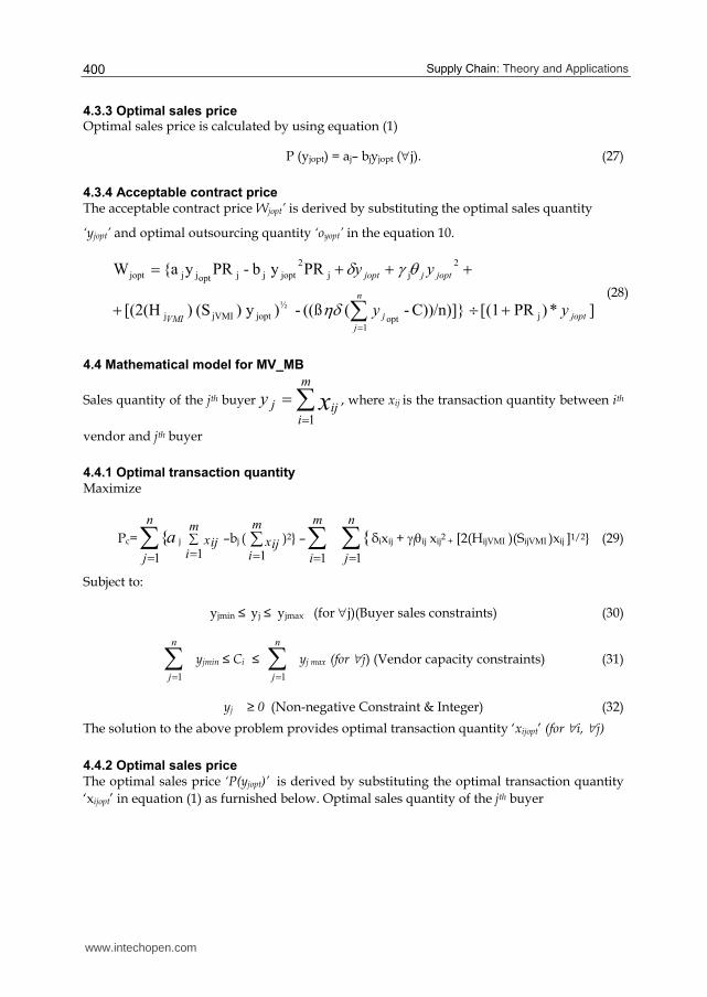
4.3.3 Optimal sales price Optimal sales price is calculated by using equation (1)
P (yjopt) = aj– bjyjopt (∀j). (27)
4.3.4 Acceptable contract price
The acceptable contract price Wjopt’ is derived by substituting the optimal sales quantity
‘yjopt’ and optimal outsourcing quantity ‘oyopt’ in the equation 10.
∑=+÷+
+++=n
j
joptjVMI
joptjjopt
yy
yy
1
jopt
½
joptjVMIj
2
jj
2
joptjjoptjjjopt
]*)PR(1[ C))/n)]}-(((ß- )y )(S )[(2(H
PRy b - PRy{aW
ηδθγδ
(28)
4.4 Mathematical model for MV_MB
Sales quantity of the jth buyer ∑== m
iijj xy
1
, where xij is the transaction quantity between ith
The solution to the above problem provides optimal transaction quantity ‘xijopt’(for ∀i, ∀j)
4.5.2 Optimal outsourcing transaction quantity
The optimal outsourcing transaction quantity is derived as follows:
Oxijopt=βij(yj- ∑=m
i 1
xijopt); (38)
where,
For every buyer ‘j’ βij =1; if the profit ratio with vendor ‘i’ is lowest; otherwise βij = 0;
www.intechopen.com
Supply Chain: Theory and Applications
402
4.5.3 Optimal sales price
The optimal sales price ‘P(yjopt)’ is derived by substituting ‘xijopt’ and ‘Oxijopt’ in equation (1) as furnished below. Optimal sales quantity of the jth buyer
∑= += m
iijoptijoptjopt )OxX(y
1
P(yjopt)= aj– bjyjopt (for ∀j) (39)
4.5.4 Acceptable contract price
The acceptable contract price ‘Wijopt’ is derived by substituting the optimal transaction quantity ‘xijopt’ and Outsourcing transaction quantity ‘Oxijopt’ in the equation 10.
)(x )PR (1
)( PR)(x b - )PROx(xa
ijoptij
ij
2
ijoptjijijoptijj
ijopt
ijoptijoptiijoptopt
ijoptOx
OxxOxW ++
+++++= δ
)(x )PR (1
)())((2)(
ijoptij
22
ijopt
ijoptijijijoptiiijoptijVMIijVMIijoptijoptijij
Ox
OxOxxSHOxx
++ ++] (++ + 1/2 θγδλθγ
(40)
5. Heuristics
Many well-known algorithmic advances in optimization have been made, but it turns out that most of them have not had the expected impact on the decisions for designing and optimizing supply chain related problems (Shapiro, 2001). For example, some optimization techniques are of little use because they are not well suited to solve complex real logistics problems in the short time, needed to make decisions. Also some techniques are highly problem-dependent and need high expertise. All the constraints of the problem may not be amenable to the mathematical articulation without such an articulation optimization may not be possible leaving the decision maker with no choice but to resort to his own experience. This adds difficulties in the implementations of optimization algorithms in the DSS which contradict the tendency to fast implementation in a rapid changing world. Alternatively for many of the problems, since the cost to find an optimal solution is so high, heuristic problem solving would suffice. Therefore, on the one hand there is the need for sophisticated logistics Decision Support System (DSS) to enable the organizations to respond quickly to new issues and problems faced on the SCM, and on the other hand there are advances in the area of heuristics that can provide an effective response to complex problems. This provides a fertile ground for applications of these techniques to SCM and subsequently of the development of computer based systems to help logistics decisions. Well-designed heuristics packages can maintain their advantage over optimization packages in terms of computer resources required, a consideration unlikely to diminish in importance so long as the size and complexity of the models arising in practice continue to increase. This is true for many areas in the firm, but especially to SCM related problems.
www.intechopen.com
Pricing in Supply Chain under Vendor Managed Inventory
403
A heuristic algorithm (often shortened to heuristic) is a solution method that does not guarantee an optimal solution, but, in general, has a good level of performance in terms of solution quality and convergence. To develop a heuristic for a particular problem, some problem-specific characteristics must be defined. The problem-specific may include the definition of a feasible solution, the neighbourhood of a solution, rules for changing solutions, and rules for setting certain parameters during the course of execution (Corne et al.,1999; Glover & Gkochenberger, 2001). In fact, some of the most popular commercial packages use heuristic methods or rules of thumb. Heuristic may be constructive (producing a single solution) or local search (starting from one or given random solutions and moving iteratively to other nearby solutions) or a combination (constructing one or more solutions and using them to start a local search). The area of heuristic techniques has been the object of intensive studies in the last decades. Recent advances in heuristic technique include meta-heuristics, which gained widespread applications along with the computational power of the computer technology. A meta-heuristic is a framework for producing heuristics, such as Simulated Annealing (SAA), Genetic Algorithm (GA), Tabu Search (TS), Particle Swarm Optimisation (PSO), Ant Colony Optimisation (ACO), etc. (Yokota et al., 1996; Costa & Oliveira 2001; Wu, 2001). Meta-heuristics have many desirable features for becoming an excellent method: in general they are simple, easy to implement, robust and have been proven highly effective to solve hard problems. Even in their most simpler and basic implementation, the meta-heuristics have been able to effectively solve very hard and complex problems. There are several aspects which are worth enough to be mentioned. The most important one is the meta-heuristics modular nature that leads to short development times and updates, given a clear advantage over other techniques for industrial applications. The other important aspect is that the amount of data involved in any optimization model for an integrated supply chain problem can be overwhelming. The complexity of the models for the SCM and the incapacity for solving in real time some of them by the traditional techniques force the use of the obvious techniques to reduce this complex issue by data aggregation (Simchi-Levi et al., 2000). Therefore, instead of aggregating data to be able to obtain a simple and solvable model, but which will not represent well the reality, researchers should consider the complex model by using an approximation algorithm. The scenario-based approaches can incorporate a meta-heuristic to obtain the best possible decision within a scenario. The combination of best characteristics of human decision-making and computerised model and algorithmic based systems into interactive and graphical design frameworks have proven to be very effective in SCM, since many supply chain problems are new, subject to rapid changes and moreover, there is no clear understanding of all of the issues involved. Rutenbar (1989) pointed out that simple heuristics is not capable of solving the hard problems with either numerous, contradictory constraints, or complex, baroque cost functions with respect to solution quality and execution time whereas meta heuristics such as GA and SAA are most suitable. SAA and GA are widely used for combinatorial optimization problems in different domains such as location, packing, partitioning and scheduling etc. SAA is a technique for combinatorial optimization problems, such as minimizing functions of very many variables. Because many real-world design problems can be cast in the form of such optimization problems, there is intense interest in general techniques for their solution. SAA is one such technique of rather recent vintage with an unusual pedigree: it is motivated by an analogy to the statistical mechanics of annealing in
www.intechopen.com
Supply Chain: Theory and Applications
404
solids. GA makes no assumptions about the function to be optimized. All that a GA requires is a performance measure, some form of problem representation, and operators that generate new population members. This general approach has been applied to many difficult and novel optimization problems. GA’s strength is its robustness, wide domain of applicability and global search capability. This modular aspect is especially important in implementing a DSS in a firm and the rapid changes that occur in the area of SCM. Lourenço (2005) pointed out that meta-heuristics, when incorporated to a DSS for SCM, can contribute significantly to the decision process, especially taking into consideration the increased complexity of the logistics problems previously presented. DSS, based on meta-heuristics, are not currently widespread, but it appears to be growing as a potential technique to solve hard problems as the one related with SCM. Taking into the above concerns, this section proposes decision support heuristics as given below in the table 1 for two echelon VMI systems considering the soft issues such as revenue sharing, pricing, real time communication, and determines the parameters such sales quantity, sales price and contract price between vendors and buyers for all two echelon environments.
S.No Environment Proposed heuristics
1 SV_SB Iterative heuristic
2 SV_MBO SAA based heuristic
3 MV_MBO GA based heuristic
Table 1 Proposed heuristics
5.1. Iterative heuristics for SV_SB problem Gjerdrum et al. (2002) addressed a method to fix fair transfer (contract) price in two enterprises SC and proposed an approach by applying the Nash bargaining principle for finding optimal multi–partner profit levels subject to given minimum echelon profit requirement. Fixation of contract price for the different revenue ratio is a tedious process, which leads to conflicts between partners, if it is not properly adopted in VMI system. Dong & Xu (2002) represented cost functions of VMI in partial differential equation and proposed a methodology to determine optimal sales quantity without giving due consideration to contract price under different revenue shares and highlighted the benefits of VMI than that of traditional mode of operation. In order to mitigate the above limitation, a new methodology is required to determine the contract prices for known revenue shares between vendor and buyer with the objective of maximizing the channel profit in two-echelon SC operating under VMI mode. The procedure should be simple and it can be easily adapted in real time by SC managers (Achabal et. al., 2000). On this concern, this chapter proposes an iterative heuristic to find optimal contract and sales prices to operate under VMI mode for the problem described in section 4.1. Though the iterative approach involves large computations, present day computers can solve them within the reasonable time. Besides this, the time factor is not much crucial to this type of offline problems. The proposed iterative heuristic involves the following two modules:
• Module 1: Determination of fair contract price (W) for various demands (y) or Sales prices (P(y)) on the assumption that they operate independently (i.e in Non VMI mode) with fair rewards or acceptable revenue shares.
• Module 2: Selection of optimal contract price (Wopt) based on the channel profits in VMI mode from various acceptable contract price (W) obtained in module 1.
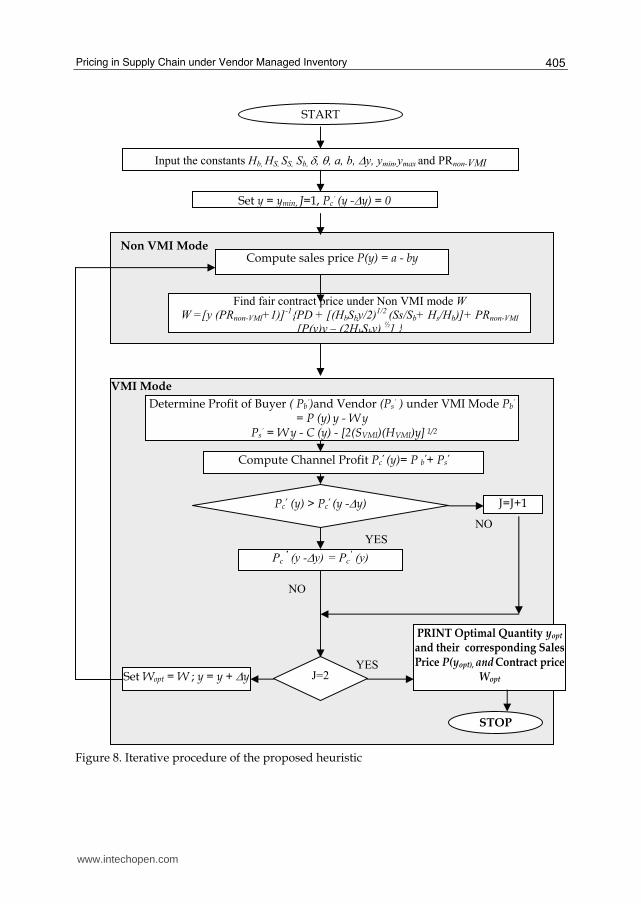
Figure 8 illustrates the mechanism of the proposed iterative heuristic.
www.intechopen.com
Pricing in Supply Chain under Vendor Managed Inventory
405
Figure 8. Iterative procedure of the proposed heuristic
Set y = ymin, J=1, Pc’ (y -Δy) = 0
START
Input the constants Hb, HS, SS, Sb, δ, θ, a, b, Δy, ymin,ymax and PRnon-VMI
Non VMI Mode Compute sales price P(y) = a - by
Find fair contract price under Non VMI mode W
W =[y (PRnon-VMI+1)]-1{PD + [(HbSby/2)1/2 (Ss/Sb+ Hs/Hb)]+ PRnon-VMI
[P(y)y – (2HbSby) ½] }
VMI Mode
Compute Channel Profit Pc’ (y)= P b’+ Ps
’
STOP
Determine Profit of Buyer ( Pb’)and Vendor (Ps’ ) under VMI Mode Pb’ = P (y) y - W y
Ps’ = W y - C (y) - [2(SVMI)(HVMI)y] 1/2
Pc’ (y) > Pc
’ (y -Δy)
Set Wopt = W ; y = y + Δy
PRINT Optimal Quantity yopt and their corresponding Sales Price P(yopt), and Contract price
Wopt
NO
J=J+1
Pc ’ (y -Δy) = Pc
’ (y)
J=2 YES
NO
YES
www.intechopen.com
Supply Chain: Theory and Applications
406
5.2 SAA Based heuristics for SV_MBO
Simulated annealing is also an intriguing technique for optimizing functions of many variables (Kirkpatrick et al., 1983). It is a heuristic strategy that provides a means for optimization of MINP problems those for which an exponentially increasing number of steps are required to generate an exact answer (Eglese, 1990). Simulated annealing is based on an analogy to the cooling of heated metals. Ponnambalam et al. (1999) states that the algorithm based on SAA, is a generalization of the well-known iterative improvement approach to combinatorial optimization problems. A generic procedure of SAA is given below in figure 9. The various steps involved in the proposed algorithm are explained below.
5.2.1 Input module
Table 2 and Table 3 serve as the input data sets to SV_MB problem. They are given as input in this module.
Maximum sales quantity y1max y2max y3max yjmax …. ynmax
Revenue Share Ratio PR1 PR2 PR3 …. PRj …. PRn
Flow cost per unit θ1 θ2 θ3 …. θj …. θn
Table 2. Buyer related data
Holding cost
Order / Setup Cost
Capacity Production Cost per unit.
Outsourcing cost constant
HS SS C δ η
Table 3. Vendor related data
5.2.2 Initialization module
Choose an initial temperature, T. The value of T is decided based upon the number of iterations to be performed. Here value of T is taken as 450 (Eglese, 1990). An initial set of sales quantity of all buyers is generated randomly with binary representation. A set of 9 digit binary numbers addresses one buyer. Each seed solution comprising of ‘n’ buyers is decoded to provide the feasible sales quantity ‘yj’ in integers by interpolating the seed information of the binary form with the following guidelines: Zero in all the nine digits
would correspond to yjmin (i.e. 000000000 ⇒ yjmin) and ‘one’ in all the nine digits would
correspond to yjmax (i.e. 111111111 ⇒ yjmax). The binary type representation and the physical meaning are as shown in figure 10.
www.intechopen.com
Pricing in Supply Chain under Vendor Managed Inventory
407
Figure 9. Flow chart representation of Simulated Annealing Algorithm process
If
∆Pc >=0
Input Module
Vendor Data: ,Ci , δi, Hsi, Ssi (∀i)
Buyer Data : n, Hbj, Sbj, aj, bj, yjmin, yjmax (∀j) ┠ij, PRjj (∀j),λ
Initialisation Module Initialize: T = 450, Iteration (ITN) = 0, α = 0.95, Accept =0 Generate: Randomly the sales quantity (yj) of all buyers in binary form with each data (yj) consisting of 9 digit binary numbers Convert: Seed in binary form to provide feasible sales quantity in integers by
quantity ‘Oxijopt’ using equation (38) based on ‘xijopt’
ii) Sales price P(yjopt) (for ∀j) using equation (39) based on the optimal quantity ‘xijopt ’
iii) Contract price wijopt (for ∀i ∀j) using equation (40) based on ‘xijopt’ and revenue share ‘PRij’
Is Termination Criterion Satisfied?
Evaluation Module Find: fitness parameter i.e. ‘fit(c)’ = ‘Pc’ Convert: ‘fit(c)’ to new fitness value suitable for maximization objective
Input Module
Vendor Data: m,Ci , δ i, HSi, SSi (for∀i)
Buyer Data : n,
Hbj, Sbj, aj, bj, yjmin, yjmax ( for∀j)
┠ij (for ∀i,∀j), PRjj (for ∀i,∀j), λi
New population generation module
Selection Find :Expected frequency of selection ‘p(c)’ Find :Cumulative probability ‘cp(c)’ Generate :random number ‘r’ Select :chromosome using ‘cp(c)’ and ‘r’ for new
population Repeat :Until the chromosome selected is equal
to pop_size
Crossover
Generate: random no. ‘r’ Select parents: ‘r’ < p_cross Cross over operator: Single point crossover.
Mutation Generate: random no. ‘r’ Select: genes having ‘r’ < p_mut Mutate: genes by replacing ‘ONE’ to ‘ZERO’ & vice versa
Initialisation Module Transaction sales quantity (yj) of all buyers in binary form with a gene (yj) consisting of 9 digit binary numbers generated chromosome to provide feasible sales quantity in integers by interpolating the
Maximum sales quantity y1max y2max y3max yjmax …. ynmax
Table 5. Buyer related data
Vendor Parameters
1 2 3 …. i …. m
Holding cost HS1 HS2 HS3 …. HSj …. HSm
Order / Setup Cost SS1 SS2 SS3 …. SSj …. SSnm
Capacity C1 C2 C3 …. Ci …. Cm
Production cost per unit δ1 δ2 δ3 …. δi δm
Outsourcing cost parameter λ1 λ2 λ3 …. λi …. λm
Table 6. Vendor related data
Buyer Parameters
Vendor
1 2 3 …. j …. n
1 PR11 PR12 PR13 …. PR1j …. PR1n
i PRi1 PRi2 PRi3 …. PRij …. PRin Revenue Share Ratio
m PRm1 PRm2 PRm3 …. Pmj …. PRmn
1 θ11 θ12 θ13 …. θ1j …. θ1n
i θi1 θi2 θi3 …. θij …. θin Flow cost per unit
m θm1 θm2 θm3 …. θmj …. θmn
Table 7. Common data between vendor and buyer
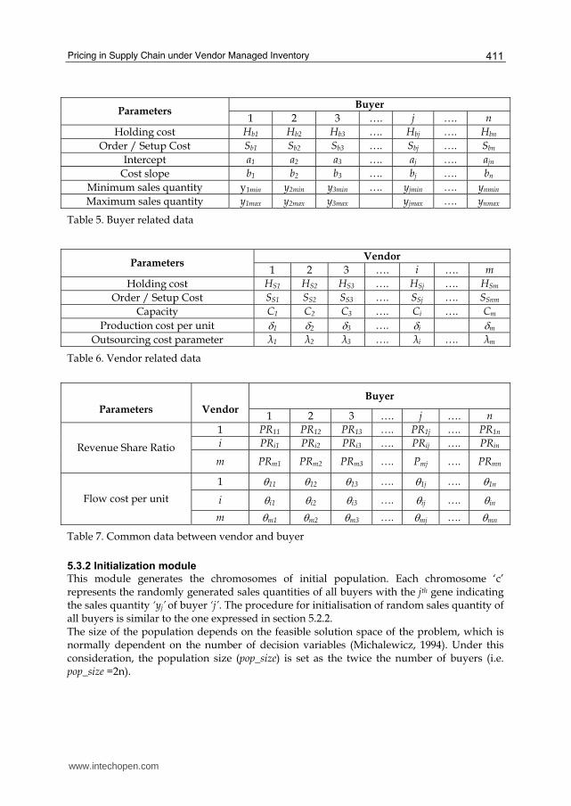
5.3.2 Initialization module
This module generates the chromosomes of initial population. Each chromosome ‘c’ represents the randomly generated sales quantities of all buyers with the jth gene indicating the sales quantity ‘yj’ of buyer ‘j’. The procedure for initialisation of random sales quantity of all buyers is similar to the one expressed in section 5.2.2. The size of the population depends on the feasible solution space of the problem, which is normally dependent on the number of decision variables (Michalewicz, 1994). Under this consideration, the population size (pop_size) is set as the twice the number of buyers (i.e. pop_size =2n).
www.intechopen.com
Supply Chain: Theory and Applications
412
5.3.3 Allocation module
In this module, the transaction quantities are allocated between the vendors and the buyers basing on the following steps i. Decoding of chromosomes: The chromosome ‘c’ is decoded to provide feasible sales
quantity (yj) (for ∀j) ii. Allocation of transaction quantity: Transaction quantity (xij) are allocated between vendor
‘i’ and buyer ‘j’ based on vendor capacity (Ci) and buyer sales quantity (yj) using north west corner rule.
5.3.4 Evaluation module
In this module, the population is evaluated and the probability of selection of each chromosome is found out. Maximisation of channel profit Pc’ is considered as an evaluation criterion. Each and every chromosome is tested for its fitness based on the following steps given below for the next generation. i. Determination of fitness parameter value: The fitness parameter ‘fit(c)’ is the channel profit
Pc and is calculated using equation (35) for chromosome ‘c’ by substituting the feasible sales quantities ‘yj’
ii. Conversion of fitness parameter value to new fitness parameter value: This step converts the fitness parameter to a new fitness value ‘newfit(c)’ suitable for the maximization objective and scaling them high, so that a very few extremely superior individuals would be selected as parents too many times. Selecting the best conversion function can be some what problem dependant. However, one function that has been found to generally useful is the exponential (Masters, 1993).
i.e., new fit(c) = e kfit(c) (42) Where k is constant and the value of the constant is usually set by trails in order to scale the fitness function reasonably to retain at least half of the good chromosomes in the population find place in the new population. Hence the new fitness parameter value is set as:
new fit(c) = e0.0005fit(C (43) iii. Conversion of new fitness to an expected frequency of selection: The final evaluation step is to
convert the new fitness parameter to an expected frequency / probability of selection (p(c)) of chromosome ‘c’ by the sum of the new fitness values of all chromosomes.
i.e., p(c) = new fit(c) / ∑==
pop_sizec
1c
newfit(c) (44)
5.3.5 Sorting module
In this module, the maximum fitness parameter is sorted out for each population and it will be stored as the local best. The maximum value is sorted out after all iterations and it is stored as the Global best.
5.3.6 Termination criterion
Termination criterion is checked after sorting module to know whether the pre-determined number of iterations is completed. On its completion, the algorithm passes to the output
www.intechopen.com
Pricing in Supply Chain under Vendor Managed Inventory
413
module, otherwise, the new set of population is generated as given in the new population generation module. The number of generations (iterations) depends upon the nature and size of the problem and is fixed by user.
5.3.7 New population generation module
Selection of next population is based on survival probability, crossover to produce children and mutation to induce external influence in new generation.
5.3.7.1 Selection module
The next population of the same size is obtained with random selection with the help of a roulette wheel procedure of which is explained here below. First the cumulative probabilities of selection / survival ‘cp(c)’ of all the chromosomes are found out.
i.e., cp(c) = ∑=
=
cc
c 1
p(c) (45)
Then the random number ‘r’ between 0 and 1 is generated and a chromosome ‘c’ is selected, satisfying the following condition:
cp(c ) ≥ r > cp(c-1) (46)
This selection process is repeated as many times as equal to population size. This method used here is more reliable because, it guarantees that most fit individuals will be selected, and that the actual number of times each chromosome selected will be within one of its expected frequency. This procedure enables fit chromosome to get multiple copies and the worst chromosome to die off.
5.3.7.2 Crossover module
This involves two steps, viz., (i) selection of chromosome for crossover and (ii) cross over operation. Probability of crossover ‘p_cross’ is a vital parameter in cross over operation. The value for p_cross is assumed as 0.6 so that atleast 60 % of chromosomes selected in the earlier selection module will undergo crossover operation and produce offspring. The procedure for this selection is as follows: Random numbers between 0 and 1 are generated for all chromosomes, and those chromosomes with random numbers less than p_ cross value are the chromosomes selected for crossover. If the number of selected chromosomes is odd, then the above procedure is repeated until one more chromosomes get selected and the number of selected chromosomes becomes an even number. The next step is to carry the crossover operation, a reproduction method. There are so many cross operations (Michalewicz, 1994). This work uses simple single point cross over. In which a cutting point is introduced at random, which splits the selected chromosomes into two parts into left and right. The right parts of the parent chromosomes are swapped to produce two new off springs. This process is continued for all the chromosomes selected for crossover.
5.3.7.3 Mutation module
The purpose of mutation is the introduction of new genetic material, or the recreation of
good genes that were lost by chance through poor selection of mates. To do this effectively,
www.intechopen.com
Supply Chain: Theory and Applications
414
the effect of mutation must be profound. At the same time, the valuable gene pool must be
protected from wanton destruction. Thus, the probability of mutation ‘p_mut’ should be tiny
(Masters, 1993). On the above grounds, the value of ‘p_mut’ is assumed as 0.03 in this
chapter. The procedure followed for mutation is as follows: Random number is generated
for each gene in the population; the genes that get random number ‘r’ less than ‘p_ mut’
undergo mutation; the selected genes are mutated by replacing ‘ONE’ to ‘ZERO’ and vice
versa.
5.3.8 Output pricing module
After completion of all iterations, the ‘global best’ fitness parameter sorted out is considered
as the optimal channel profit ‘Pcopt’ and its corresponding optimal sales quantity of all buyers
is ‘yjopt’. This module derives the optimal sales price ‘P(yjopt)’ and acceptable contract price
‘Wjopt’ for the optimal quantity ‘yjopt’ determined from the previous module. Sales price for
each buyer is calculated using the equation (39) and contact price for each buyer is
calculated using equation (40). Complete output obtained is shown in Table 8 for the
This section illustrates the GA based heuristic proposed for MV_MBO model with a pilot
study data from agricultural development offices situated at three rural places of south
India. The landowners (vendor) supply rice grains to these agricultural development offices.
The agricultural development offices (buyers) supply their products (rice grains) to the
customers. This section illustrates the proposed methodology only with 2 vendors and three
buyers and it can as well be extended, to ‘m’ vendors and ‘n’ buyers. The vendor is currently
operating in independent mode where the buyers initiate the orders everyday. Based on the
orders, the vendors supply the required quantities to buyers. Table 9, 10 and 11 provide the
buyer related data, vendor related data and the common data between vendor and buyers
respectively.
www.intechopen.com
Pricing in Supply Chain under Vendor Managed Inventory
415
yj 1 2 3
Hbj 2 1 2
Sbj 5 5 7
aj 23 22 21
bj 0.0001 0.0002 0.0003
yjmin 1000 2000 1000
yjmax 2000 3000 3000
Table 9. Buyer related data
i Hsi Ssi Ci δi λi
1 2 10 3000 15 0.2
2 1 9 3000 16 0.2
Table 10. Vendor related data
j Parameters
I
1 2 3
1 1.2 1.1 1.3 PRij 2 1.2 1.2 1.1
1 0.004 0.002 0.005 θij 2 0.005 0.003 0.002
Table 11. Common data between vendor and buyer
Various modules of the GA heuristic are shown in Tables 12 to 19 respectively, and the optimal parameters for the case problem are shown in Tables 20. The GA parameters used are as follows: chromosome length = 27, pop_size =12, p_cross = 0.6, p_mut=0.03, number of iterations = 100.
This section reports the robustness of the model and methodology, limitation, in the current research, managerial implications and potential scope for future research. This chapter addressed to the soft issues of profit sharing and pricing in SCM and has concentrated on development of decision support heuristics to determine the optimal or near optimal operational parameters (Sales quantities, Prices (sales and contract) and outsourcing quantities and transaction quantities) for maximum channel profit to the two-echelon SC models operating under VMI mode. i. Single Vendor Single Buyer (SV_SB) ii. Single Vendor Multiple Buyer’s (SV_MB) iii. Multiple Vendors Multiple Buyers (MV_MB) iv. Single Vendor Multiple Buyer’s with Outsourcing (SV_MBO) v. Multiple Vendors Multiple Buyers with Outsourcing (MV_MBO) Furthermore, this chapter illustrated application of VMI systems for two-echelon SC models in the agricultural sector. Fixation of contract price for the different revenue ratio is a tedious process, which leads to conflicts between partners, if it is not properly adopted in VMI system. To overcome the above limitation, a new methodology is required to determine the contract prices for known revenue shares between vendor and buyer. Hence, this chapter proposes an iterative heuristic procedure for SV_SB model to find optimal or near optimal operational parameters. The mathematical formulation of the remaining four models (SV_MB, MV_MB, SV_MBO, MV_MBO) belongs to Nonlinear Integer Programming (NIP) and Mixed Integer Nonlinear Programming (MINP) problems. The Hessian matrix of the objective functions confirms the nature of it as non-convex. Hence GA and SAA based heuristics are proposed to solve the above models. Iterative heuristic procedure provides optimal/near optimal solution when compared with the methodology proposed by Dong & Xu (2002) for the same SV_SB operating in VMI mode of operation, but under equal revenue share cases. GA and SAA based heuristics provides near optimal solution when compared with i) LINGO optimization solver for smaller size problems ii) DX methodology of Dong & Xu (2002) by reducing the models (2-5) into SV_SB. The computational time increases with increase in number of vendors and buyers. However the problem is static and justifiable. The robustness of the models are evaluated by changing the influencing parameters such as limits on sales quantity, slope of demand function, cost of holding and cost of setup/order. Variation in holding and order setup cost has less impact in sales quantities, sales price and
www.intechopen.com
Pricing in Supply Chain under Vendor Managed Inventory
419
contract price, whereas it has more impact on the channel profit. Variations in limits on sales quantity and slope of demand pattern have more impact on operational parameters and channel profit. Hence it is concluded that the model presented, the heuristics proposed and the analysis carried out in this chapter work would aid SC managers to take appropriate decision in two- echelon VMI systems.
7.2 Future directions • Inventory holding cost and order setup cost for vendor in all the above models are assumed as sum of both holding cost and order setup cost, but in practice the inventory cost will be less. Therefore the vendor profit and channel profit would be more in real time. Future analysis can consider various combination of inventory holding and order setup cost to the above models and the insight of the problem could be studied.
• The distribution cost in all the models varies parabolically depending upon the increase in quantity and mode of transportation. Since in VMI, the vendor has to monitor inventory and to replenish products as and when required, there will be exponential variation in distribution cost depending upon the increase in quantity and mode of transportation. Hence future research can represent distribution cost with respect to product and incorporate fixed transportation cost to depict the real cost of transportation.
• All the above models assume reverse linear relationship between price-sales quantities. The impact on optimal operational parameters for various demand curves can be studied for other categories of product.
• The mode of operation assumes zero lead time and would not allow backlog and stock out. Researchers in future can accommodate these factors along with shortage cost for varying service levels while developing two-echelon models.
• Concept of heuristics proposed for two-echelon models could be extended for multi echelon models
• This chapter illustrated the development of heuristics for sectors like agriculture, but this can be extended to any kind of product and service sectors such as milk, engineering services etc.
• Development of knowledge managed systems for two-echelon VMI systems to determine operational parameters for maximum channel profit based on the experts experience and with the data available from the market.
• The other soft issues such as organizational resistance to change, inter-functional conflicts, team oriented performance measures and channel power shift have not been considered while modelling two-echelon SC. Hence future researchers may pay more attention to these issues.
8. Acknowledgement
The authors thank the Management, the Principal, and the Head of Mechanical Engineering Department of Thiagarajar College of Engineering, Madurai, India and the Nottingham University Business School, Nottingham, UK for providing necessary facilities to carry out this work. The authors specially thank Department of Science and Technology (SERC Division), New Delhi for the BOYSCAST fellowship (SR/BY/E-09/06) to carry out this research work at Nottingham University and All India Council for Technical Education
www.intechopen.com
Supply Chain: Theory and Applications
420
(F.No. 1-51/FD/CA/(16) 2006-07 dated 12/12/2006) for the career award for the young teachers offered to the first author.
9. References
Achabal, D.D., Mcintyre, S.H., Smith & S.A., Kalyanam, K. (2000). A Decision support system for VMI. Journal of Retailing, 76(4), 430 -54.
Banerjee A. (1986). A joint economic lot size model for purchaser and vendor. Decision Science, 17, 292-311.
Ballou, R. H., Gilbert, S. M. & Mukherjee, A. (2000). New managerial challenges from supply chain opportunities. Industrial Marketing Management, 29, 7–18.
Bhattacharjee, S & Ramesh, R. (2000). A multi-period profit maximizing model for retail supply chain management: An integration of demand and supply side mechanism. European Journal of Operational Research, 122, 584-601.
Burke, M. (1996). Its Time for Vendor Managed Inventory. Industrial Distribution. 85-90. Cachon, G.P., (2001). Stock wars: Inventory competition in a two-echelon supply chain with
multiple retailers. Operations Research, 49(5), 658-74. Cachon, G.P & Zipkin, P.H. (1999). Competitive and cooperative Inventory Policies in a two
stage supply chain. Management science, 45(7), 936-953. Casati, F., Dayal, U & Shan. M-C. (2001). E Business Applications for Supply Chain
Management: Challenges and Solutions. IEEE Journal, 1063-6382 / 01, 71-78. Cetinkaya, S. & Lee C. Y. (2000). Stock Replenishment and Shipment Scheduling For
Vendor-Managed Inventory Systems. Management Science, 46(2), 217-232. Chopra, S. (2003). Designing the Distribution Networks in a supply Chain. Transportation
Research-Part E, 39, 123-140. Clark, T.H. & Croson, D.C. (1994). H.E. Butt Grocery Company: a leader in ECR
implementation. Harvard Business School Case, 9, 195-125. Corne D., Dorigo M. & Glover F. (1999). New Ideas in Optimisation. McGraw-Hill. Costa, L. & Oliveira, P. (2001). Evolutionary algorithms approach to the solution of mixed
integer nonlinear programming problems. Computers and Chemical Engineering, 25, 257-66.
Desarbo, W.S., Rao, V.R., Steckel, J.H., Wind, J. & Colombo, R., (1987). A Friction model for describing and forecasting price changes. Journal of Marketing Science, 6 (4), 299-319.
Disney, S.M. & Towill, D.R. (2003). Vendor managed inventory and bull whip reduction in a two level supply chain. International Journal of Operations and Production Management. 23(6), 625-651.
Disney, S.M. & Towill, D. R. (2002). A procedure for optimization of the dynamic response of a Vendor Managed Inventory system. Computers and Industrial Engineering, 43, 27-58.
Dong, Y. & Xu, K. (2002). A supply chain model of vendor managed inventory. Transportation Research Part E: Logistics and Transportation Review, 38(2), 75–95.
Eglese, R.W., (1990). Simulated Annealing: A tool for Operational Research. European Journal of Operational Research, 271-281.
Fry, M.J. (2002). Collaborative and cooperative agreement in the supply chain, Ph.D. Thesis report, University of Michigan.
Gallego, G. & Vanryzin, G. (1994). Optimal Dynamic Pricing of Inventories with Stochastic demand Over Finite Horizons. Management Science, 40, 999-1020.
www.intechopen.com
Pricing in Supply Chain under Vendor Managed Inventory
421
Ganeshan,R. (1999). Managing supply chain inventories: A multiple retailer, one warehouse, multiple supplier model. International Journal of Production Economics, 59, 341-54.
Gavirneni, S., (2001). Benefits of cooperation in a production distribution environment. European Journal of Operational Research, 130(3), 612 – 22.
Giannoccaro, I. & Pontrandolfo, P. (2004). Supply Chain Coordination by revenue sharing contracts. International Journal of Production Economics, 89, 131-139.
Gjerdrum , J., Shah, N. & Papageorgiou, L.G. (2002). Fair Transfer Price and Inventory holding policies in Two Enterprise Supply Chains. European Journal of Operational Research, 143, 582 – 599.
Glover, F & Gkochenberger, G (2001). (eds.) Handbook in Meta heuristics. Kluwer Academic Publishers.
Grieger, M. (2003). Electronic marketplaces: A literature review and a Call for Supply chain management research. European Journal of Operational Research, 144, 280–294.
Goyal, S. K., 1997. An integrated inventory model for a single supplier-single customer problem. International Journal of Production Research, 15, 107-111.
Goyal, S.K. & Nebebe,F. (2000). Determination of economic production- shipment policy for a single-vendor-single-buyer system. European Journal of Operational Research 121, 175-178.
Hammond, J.H, (1990). Quick response in the apparel industry. Harvard Business School Note N9-690-038, Cambridge, MA.
Hill, R.M. (1997). The single-vendor single-buyer integrated production-inventory model with a generalised policy. European Journal of Operational Research, 97, 493-499.
Hoque, M.A & Goyal, S.K, (2000). An optimal policy for a single-vendor single-buyer integrated production-inventory system with capacity constraint of the transport equipment. International Journal of Production Economics 65, 305-315.
Klastorin, T. (2004). New Product Introduction: Timing, Design, and Pricing. Manufacturing and Service Operations Management 6(4), 302–320.
Lau, A.H.L. & Lau. H-S. (2003). Effects of a demand curve’s shape on the optimal solutions of a multi echelon inventory / pricing model. European Journal of Operations Research 147, 530-548.
Latamore & Benton,G., 1999. The farm business unit customers; Customers, Suppliers Drawing Closer through VMI. APICS: The Performance Advantage, 12(7), 22-25.
Lee, C.C & Chu, W.H.J., 2005. Who should control inventory in a supply chain. European Journal of Operational Research, 164(1), 158-72.
Lourenco, H.R. (2005). Logistics Management: an opportunity for Metaheuristics, in Metaheuristics Optimization via Memory and Evolution. C. Rego and B. Alidaee (eds.), Kluwer Academic Publishers, 329-356.
Lu, L. (1995). A one-vendor multi-buyer integrated inventory model. European Journal of Operational Research, 81(2), 312-23.
Mabert, V. A. & Venkataramanan, M.A. (1998). Special Research Focus on Supply Chain Linkages: Challenges for Design and Management in the 21st Century, Decision Sciences, 29(3), 537-552.
Mccall, J., (2005). Genetic algorithms for modelling and optimisation. Journal of Computational and Applied Mathematics, 184(1), 205-222.
www.intechopen.com
Supply Chain: Theory and Applications
422
Maloni, M.J & Benton, W.C. (1997). Supply Chain Partnership: Opportunities for Operations Research. European Journal of Operational Research 101, 419-429.
Masters, T. (1993). Practical Neural Network Recipes in C++. NewYork, Academic Press. Michalewicz, Z. (1994). Genetic Algorithms + Data Structures = Evolution Programs. 2nd Edition,
Springer, Berlin. Min, H. & Zhou, G. (2002). Supply chain modelling: past, present and future. Computers and
Industrial Engineering 43,231-249. Minner, S., (2003). Multiple-supplier inventory models in supply chain management: A
review. International Journal of Production Economics 81-82, 265-79. Mishra, B.K., & Raghunathan, S. (2004). Retailer vs. Vendor Managed Inventory and Brand
Competition. Management Science 50(4), 445-457. Nachiappan, SP., Jawahar, N. & Ganesh, M., (2006). Pricing in Vendor Managed Inventory
Systems. International Journal of Logistics Systems and Management, 2(1), 19- 40. Nachiappan, SP., Gunasekaran, A., & Jawahar, N. (2007). Knowledge management system
for operating parameters in two-echelon VMI supply chains. International Journal of Production Research 45(11), 2479–2505.
Nachiappan, SP.& Jawahar, N. (2007). A genetic algorithm for optimal operating parameters of VMI system in a two-echelon supply chain. European Journal of Operational Research 183(3), 1433-1452.
Nachiappan, SP., Jawahar, N. & Arunkumar, A.C (2007a). Evolution of operating parameters for a Multiple Vendors and Multiple Buyers Vendor Managed Inventory System with outsourcing using Simulated Annealing Algorithm. International Journal of Industrial Management and Optimization, 3(3), 597-618.
Parks, L. & Popolillo, M.C (1999). Co-Managed Inventory is focus of Vendor/ Retailer Pilot. Drug Store News, 27, 71.
Polatoglu, L.H. (1991). Optimal order quantity and pricing decisions in single period inventory systems. International Journal of Production Economics, 23, 175-185.
Ponnambalam, S.G., Jawahar, N. & Aravindan, P. (1999). A simulated annealing algorithm for job shop scheduling. Production planning and control, 10, 767-777.
Ravindran, A., Phillips, D.T. & Solberg, J.J., (2000). Operations Research: Principles and Practice. 2nd edition; New York: John Wiley & Sons.
Rajan, A., Rakesh, A & Steinberg, R. (1992). Dynamic pricing and ordering decisions by a monopolist. Management Science 38, 240-262.
Rutenbar, R.A. (1989). Simulated annealing algorithms: An overview. IEEE Circuits and Devices Magazine, 19-26.
Sedarage, D., Fujiwara, O & Luong, H.T., (1999). Determining optimal order splitting and reorder level for N-supplier inventory systems. European Journal of Operational Research, 116, 389-404.
Simchi-Levi D., Kaminsky, P. & Simchi-Levi, E. (2000). Designing and Managing the Supply Chain, McGraw-Hill.
Shapiro, J. F., (2001). Modeling the supply chain, Pacific Grove, CA: Wadsworth Group Tronstad, R. (1995). Pricing. Journal of Market Analysis and Pricing, 39 -45. Viswanathan, S. (1998). Optimal strategy for the integrated vendor-buyer inventory model.
European Journal of Operational Research 105(1), 38-42. Waller, M., Johnson, M.E.& Davis, T. (2001). Vendor managed inventory in the retail supply
chain. Journal of Business Logistics 20(1), 183-203.
www.intechopen.com
Pricing in Supply Chain under Vendor Managed Inventory
423
Williams, M.K. (2000). Making Consignment and Vendor Managed Inventory work for you. Hospital Material Management Quarterly, 21(4), 59-63.
Yao, M.J & Chiou,C.C.(2004). On a replenishment coordination model in an integrated supply chain with one vendor and multiple buyers. European Journal of Operational Research 159, 406–419.
Yokota,T., Gen, M. & Li. Y.X. (1996). Genetic Algorithm for non linear mixed integer programming problems and its applications. Computers and Industrial Engineering 30(4), 905 – 17.
Nomenclature
a Constant.
aj Intercept value for the demand pattern of the jth buyer
b Slope of Demand pattern – Selling Price Curve.
bj Cost Slope of the demand pattern of the jth buyer
c, c’ ,c’’, c’’’ Chromosome
C Capacity of the vendor
Ci Capacity of the vendor ‘i’
cp(c ) Cumulative probability of survival
cp(c-1) Cumulative probability of survival of previous chromosome
EOQ Economic order quantity
EOQj Economic order quantity of jth buyer
EOQij Economic order quantity from ith vendor to jth buyer
F Frame work
fit(c) Fitness function
Hb Holding cost per unit per unit time of the buyer in independent mode of operation.
Hbj Holding cost of the jth buyer in independent mode
HS Holding cost per unit per unit time of the vendor in independent mode of operation.
HSi Holding cost of the vendor ‘i’ in independent mode
HVMI Inventory cost of vendor per unit per unit time in VMI mode of operation.
HjVMI Holding cost of the vendor in VMI mode
HijVMI Holding cost of the vendor ‘i’ to jth buyer in VMI mode
i Vendor identifier (i= 1 to m)
j Increment factor for sales quantity.
m Number of vendors
n Number of the buyers
newfit(c) New fitness function
OSM Order and stock maintenance cost to the vendor for buyer
www.intechopen.com
Supply Chain: Theory and Applications
424
OSMj Order and stock maintenance cost to the vendor for each buyer
OSMij Order and stock maintenance cost to the vendor ‘i’ for each buyer ‘j’
Ox Outsourcing transaction quantity
Oxij Outsourcing transaction quantities between vendor ‘i’ and buyer ‘j’
Oxijmin Minimum outsourcing transaction quantities between vendor ‘i’ and buyer ‘j’
Oxijmax Maximum outsourcing transaction quantities between vendor ‘i’ and buyer ‘j’
Oxijopt Optimal outsourcing transaction quantities between vendor ‘i’ and buyer ‘j’
OCxij Outsourcing cost from ith vendor to jth buyer
oy Outsourcing quantity
oyopt Optimal outsourcing quantities
oc Outsourcing cost of the vendor
ocj Outsourcing cost of the vendor to jth buyer (ocj=oc/n)
p_cross Probability of the cross over
P Pricing
P b Buyer Profit under Independent mode of operation
P b’ Buyer Profit in VMI mode
Pbj Profit of jth buyer in VMI mode
Pc Channel profit in independent mode
Pc’ Channel profit in VMI mode
Pc’’ Channel profit obtained after perturbation in Simulated annealing
∆ Pc Difference in Channel Profit
Pcopt Optimal channel profit in VMI mode
Ps Vendor Profit under Independent mode of operation.
Ps’ Vendor Profit in VMI mode
Psi Profit of vendor ‘i’ in VMI mode
Psj Profit obtained by vendor when supplying products to the buyer ‘j’ in VMI mode
Psij Profit obtained by vendor ‘i’ when supplying products to the buyer ‘j’
PD Production distribution cost of the buyer.
PDj Production distribution cost of the jth buyer.
PDij Production distribution cost from ith vendor to the jth buyer.
p(c) Probability of survival of chromosome ‘c’
p_mut Probability of mutation
pop_size Population size
P(y) Sales Price
www.intechopen.com
Pricing in Supply Chain under Vendor Managed Inventory
425
P(yj) Sales price of the jth buyer corresponding to sales quantity ‘yj’
P(yopt) Sales price at optimal sales quantity y opt.
P(yjopt) Optimal sales price of the jth buyer
PR non-VMI Revenue share ratio between vendor and buyer when they operate under non -VMI mode (Ps/ P b).
PR Revenue share ratio between vendor and buyer when they operate under VMI mode (Ps’/ P b’).
PRj Revenue share ratio between vendor and the jth buyer
PRij Revenue share ratio between ith vendor and the jth buyer
Pc’ (y) Channel Profit for quantity y in VMI mode of operation.
Pc’(y -Δy) Channel Profit of VMI mode for the prior incremental value of sales quantity
Q Replenishment quantity
Qj Replenishment quantity to each buyer ‘j’
Qij Replenishment quantity from vendor ‘i’ to buyer ‘j’
r Random number
Sb Setup cost per order of the buyer in Independent mode of operation.
Sbj Setup cost of the jth buyer per order in independent mode
SS Setup cost of the vendor per order in independent mode
SSi Setup cost of the vendor ‘i’ per order in independent mode
SVMI Set up cost per order of the vendor in VMI mode of operation.
SjVMI Setup cost of the vendor per order in VMI mode of operation to buyer ‘j’
SijVMI Setup cost of the vendor ‘i’ per order in VMI mode of operation to buyer ‘j’
T Temperature
t1,t2 Random numbers generated in Simulated Annealing for perturbation
W Contract price
Wj Contract price between vendor and buyer ‘j’
Wij Contract price between vendor ‘i’ and buyer ‘j’
Wopt Optimal Contract price.
Wjopt Optimal contract price between vendor and buyer ‘j’
Wijopt Optimal contract price between vendor ‘i’ and buyer ‘j’
x Transaction quantity
xij Transaction quantities between vendor ‘i’ and buyer ‘j’
ximin Minimum transaction quantities between vendor ‘i’ and buyer ‘j’
xijmax Maximum transaction quantities between vendor ‘i’ and buyer ‘j’
xijopt Optimal transaction quantities between vendor ‘i’ and buyer ‘j’
y Sales quantity
www.intechopen.com
Supply Chain: Theory and Applications
426
yj
Sales quantity of the jth buyer (i.e.∑== m
iijj xy
1 )
Y Aggregate sales quantity of the vendor (i.e. y=
yj
n
j
∑=1 )
yi
Aggregate sales quantity of the vendor ‘i’ (i.e. yi=y
j
n
j
∑=1 )
yj’ Sales quantity obtained after perturbation in Simulated annealing of the jth buyer
ymin Minimum expected sales quantity.
yj min Minimum expected sales quantity of the jth buyer
ymax Maximum expected sales quantity
yj max Maximum expected sales quantity of the jth buyer
yopt Optimal sales quantity.
yjopt Optimal sales quantity of the jth buyer
θ Flow cost per unit from vendor to buyer.
θj Flow cost per unit from vendor to buyer ‘j’
θij Flow cost per unit from vendor ‘i’ to buyer ‘j’
υ Transportation resource cost per unit from vendor to buyer
υj Transportation resource cost per unit from vendor to buyer ‘j’
υij Transportation resource cost per unit from vendor ‘i’ to buyer ‘j’
δ Production cost per unit
δi Production cost per unit for vendor ‘i’
┙ Temperature factor
┚ Outsourcing factor
Δy Incremental change in sales quantity
βij Outsourcing factor between vendor ‘i’ and buyer ‘j’
η Outsourcing cost constant
λ Additional outsourcing cost
λi Additional outsourcing cost for vendor ‘i’
www.intechopen.com
Supply ChainEdited by Vedran Kordic
ISBN 978-3-902613-22-6Hard cover, 568 pagesPublisher I-Tech Education and PublishingPublished online 01, February, 2008Published in print edition February, 2008
InTech ChinaUnit 405, Office Block, Hotel Equatorial Shanghai No.65, Yan An Road (West), Shanghai, 200040, China
Phone: +86-21-62489820 Fax: +86-21-62489821
Traditionally supply chain management has meant factories, assembly lines, warehouses, transportationvehicles, and time sheets. Modern supply chain management is a highly complex, multidimensional problemset with virtually endless number of variables for optimization. An Internet enabled supply chain may have just-in-time delivery, precise inventory visibility, and up-to-the-minute distribution-tracking capabilities. Technologyadvances have enabled supply chains to become strategic weapons that can help avoid disasters, lower costs,and make money. From internal enterprise processes to external business transactions with suppliers,transporters, channels and end-users marks the wide range of challenges researchers have to handle. Theaim of this book is at revealing and illustrating this diversity in terms of scientific and theoretical fundamentals,prevailing concepts as well as current practical applications.
How to referenceIn order to correctly reference this scholarly work, feel free to copy and paste the following:
Subramanian Nachiappan and Natarajan Jawahar (2008). Pricing in Supply Chain under Vendor ManagedInventory, Supply Chain, Vedran Kordic (Ed.), ISBN: 978-3-902613-22-6, InTech, Available from:http://www.intechopen.com/books/supply_chain/pricing_in_supply_chain_under_vendor_managed_inventory