Pricing models for Bermudan-style interest rate derivatives · Pricing models for Bermudan-style...

Pricing models for Bermudan-style interest ratederivatives Bermudan-style interest rate derivatives are an important class of

options. Many banking and insurance products, such as mortgages,

cancellable bonds, and life insurance products, contain Bermudan

interest rate options associated with early redemption or cancella-

tion of the contract. The abundance of these options makes evident

that their proper valuation and risk measurement are important to

banks and insurance companies. Risk measurement allows for off-

setting market risk by hedging with underlying liquidly traded assets

and options. Pricing models must be arbitrage-free, and consistent

with (calibrated to) prices of actively traded underlying options.

Model dynamics need be consistent with the observed dynamics of

the term structure of interest rates, e.g., correlation between inte-

rest rates. Moreover, valuation algorithms need be efficient: Finan-

cial decisions based on derivatives pricing calculations often need to

be made in seconds, rather than hours or days. In recent years, a

successful class of models has appeared in the literature known as

market models. This thesis extends the theory of market models, in

the following ways: (i) it introduces a new, efficient, and more

accurate approximate pricing technique, (ii) it presents two new and

fast algorithms for correlation-calibration, (iii) it develops new models

that enable efficient calibration for a whole new range of deriva-

tives, such as fixed-maturity Bermudan swaptions, and (iv) it presents

novel empirical comparisons of the performance of existing calibra-

tion techniques and models, in terms of reduction of risk.

ERIMThe Erasmus Research Institute of Management (ERIM) is the Research

School (Onderzoekschool) in the field of management of the

Erasmus University Rotterdam. The founding participants of ERIM

are RSM Erasmus University and the Erasmus School of Economics.

ERIM was founded in 1999 and is officially accredited by the Royal

Netherlands Academy of Arts and Sciences (KNAW). The research

undertaken by ERIM is focussed on the management of the firm in its

environment, its intra- and inter-firm relations, and its business

processes in their interdependent connections.

The objective of ERIM is to carry out first rate research in manage-

ment, and to offer an advanced graduate program in Research in

Management. Within ERIM, over two hundred senior researchers and

Ph.D. candidates are active in the different research programs. From

a variety of academic backgrounds and expertises, the ERIM commu-

nity is united in striving for excellence and working at the forefront

of creating new business knowledge.

www.erim.eur.nl ISBN 90-5892-099-2

RAOUL PIETERSZ

Pricing models forBermudan-styleinterest rate derivatives

Desig

n: B

&T O

ntw

erp en

advies w

ww

.b-en

-t.nl

Print:H

aveka ww

w.h

aveka.nl

71

RA

OU

L P

IET

ER

SZ

Pricin

g m

od

els fo

r Be

rmu

da

n-sty

le in

tere

st rate

de

riva

tive

s

Erim - 05 omslag Pietersz 9/23/05 1:41 PM Pagina 1

1

Pricing Models for Bermudan-StyleInterest Rate Derivatives

2

3

Pricing Models for Bermudan-StyleInterest Rate Derivatives

Waarderingsmodellen voor Bermuda-stijl rente derivaten

Proefschrift

ter verkrijging van de graad van doctor aan de

Erasmus Universiteit Rotterdam

op gezag van de

rector magnificus

Prof.dr. S.W.J. Lamberts

en volgens besluit van het College voor Promoties.

De openbare verdediging zal plaatsvinden op

donderdag 8 december 2005 om 16.00 uur

door

Raoul Pietersz

geboren te Rotterdam

4

Promotiecommissie

Promotoren:

Prof.dr. A.A.J. Pelsser

Prof.dr. A.C.F. Vorst

Overige leden:

Prof.dr. P.J.F. Groenen

Prof.dr. F.C.J.M. de Jong

Dr.ir. M.P.E. Martens

Erasmus Research Institute of Management (ERIM)

Erasmus University Rotterdam

Internet: http://www.erim.eur.nl

ERIM Ph.D. Series Research in Management 71

ISBN 90-5892-099-2

c© 2005, Raoul Pietersz

All rights reserved. No part of this publication may be reproduced or transmitted in

any form or by any means electronic or mechanical, including photocopying, recording,

or by any information storage and retrieval system, without permission in writing from

the author.

5

Voor Beata, Karsten en Daniel

6

7

Acknowledgements

First and foremost, I would like to thank my promotor Antoon Pelsser. His guidance

throughout the Ph.D. period has been excellent. Chapters 2, 5 and 6 were written in

cooperation with Antoon. The research benefitted greatly from his invaluable suggestions,

and he truly is an inspirator. Thank you Antoon.

Second, I thank my promotor and former employer Ton Vorst. He is the one who

suggested me to start the Ph.D. track with Antoon Pelsser, and who part-time employed

me at ABN AMRO Bank, Quantitative Risk Analytics (at the time “Market Risk –

Modelling and Product Analysis”), for the period September 2001 till June 2004. For all

this, I am very grateful.

Third, many thanks go to the other members of the small committee; Patrick Groenen,

Frank de Jong, and, Martin Martens. Also, I express my gratitude to the other members

of the committee; Lane Hughston, Farshid Jamshidian, and, Thierry Post.

Fourth, special thanks go to Marcel van Regenmortel, for teaching me many technical

and exciting aspects of interest rate derivatives pricing, and for part-time employing me

at Product Development Group, Quantitative Analytics, ABN AMRO Bank, from July

2004 onwards. Chapters 5 and 7 were written in cooperation with Marcel.

Fifth, I am grateful to Patrick Groenen, for co-authoring Chapter 3.

Sixth, I thank Igor Grubisic for co-authoring Chapter 4.

I am much obliged to my colleagues at Erasmus University Rotterdam: Jaap Spronk

for support through the Erasmus Center for Financial Research (ECFR); Martin Martens

for his help while I was co-teaching one of his example classes and for suggesting me

as a lecturer at the Rotterdam School of Management (RSM); Winfried Hallerbach for

help with preparation of RSM lectures; Wilfred Mijnhardt for guiding me through the

publication process; Tineke Kurtz, Tineke van der Vhee, Elli Hoek van Dijke, and Ella

Boniuk, for efficiently aiding me in administrative matters; and, Marielle Sonnenberg, for

being a pleasant room-mate.

During the Ph.D. period I have been able to present my work at leading international

conferences. I am very grateful for the financial support that made this possible, received

from Erasmus Research Institute of Management (ERIM), from the Econometric Institute

(EI), and from ECFR.

8

viii ACKNOWLEDGEMENTS

A special thank you to past and present managers at ABN AMRO Bank: Ton Vorst,

Dick Boswinkel, Nam Kyoo Boots, Marcel van Regenmortel, Bernt van Linder and Geert

Ceuppens. Thank you to past and present colleagues at Product Development Group:

Nicolas Carre in Amsterdam, and Thilo Roßberg and Russell Barker in London. Thanks to

members of CAL: Nancy Appels, Reinier Bosman, Danny Wester, Frank Putman, Andre

Roukema, Jelper Striet, and Willem van der Zwart. Thank you to past and present

colleagues at ‘Product Analysis’: Steffen Lukas, Benjamin Schiessle, Martijn van der

Voort, Lukas Phaf, Alice Gee, Rutger Pijls, Drona Kandhai, and Alex Zilber. A thank

you to colleagues that have become friends: Dion Hautvast, Bram Warmenhoven, and

Glyn Baker.

I am also grateful to a number of anonymous referees and to Riccardo Rebonato and

Mark Joshi who provided valuable comments and suggestions to earlier versions of the

papers that form the basis for this thesis. Many thanks to Frank de Jong and Joanne

Kennedy for providing much appreciated feedback to my research proposal.

Finally, I would like to thank my parents for always being there for me. I thank my

son Karsten for bringing so much joy to my life. I thank Beata for her love, support, and

kindness.

Raoul Pietersz

February 7th 2005, Amsterdam

9

Contents

Acknowledgements vii

Notation xix

Outline xxiii

1 Introduction 1

1.1 Arbitrage-free pricing . . . . . . . . . . . . . . . . . . . . . . . . . . . . . . 1

1.1.1 Use of models in practice . . . . . . . . . . . . . . . . . . . . . . . . 4

1.2 Interest rate markets and options . . . . . . . . . . . . . . . . . . . . . . . 6

1.2.1 Linear products: Deposits, bonds, and swaps . . . . . . . . . . . . . 7

1.2.2 Interest rate options: Caps, floors, and swaptions . . . . . . . . . . 8

1.3 Interest rate derivatives pricing models . . . . . . . . . . . . . . . . . . . . 11

1.3.1 Short rate models . . . . . . . . . . . . . . . . . . . . . . . . . . . . 12

1.3.2 Market models . . . . . . . . . . . . . . . . . . . . . . . . . . . . . 15

1.3.3 Markov-functional models . . . . . . . . . . . . . . . . . . . . . . . 16

1.4 American option pricing with Monte Carlo simulation . . . . . . . . . . . . 17

2 Risk-managing Bermudan swaptions in a LIBOR model 19

2.1 Introduction . . . . . . . . . . . . . . . . . . . . . . . . . . . . . . . . . . . 19

2.2 Recalibration approach . . . . . . . . . . . . . . . . . . . . . . . . . . . . . 21

2.3 Explanation . . . . . . . . . . . . . . . . . . . . . . . . . . . . . . . . . . . 24

2.4 Swap vega and the swap market model . . . . . . . . . . . . . . . . . . . . 27

2.5 Alternative method for calculating swap vega . . . . . . . . . . . . . . . . 29

2.6 Numerical results . . . . . . . . . . . . . . . . . . . . . . . . . . . . . . . . 30

2.7 Comparison with the swap market model . . . . . . . . . . . . . . . . . . . 30

2.8 Conclusions . . . . . . . . . . . . . . . . . . . . . . . . . . . . . . . . . . . 32

2.A Appendix: Negative vega two-stock Bermudan options . . . . . . . . . . . 34

10

x CONTENTS

3 Rank reduction of correlation matrices by majorization 39

3.1 Introduction . . . . . . . . . . . . . . . . . . . . . . . . . . . . . . . . . . . 39

3.2 Literature review . . . . . . . . . . . . . . . . . . . . . . . . . . . . . . . . 43

3.2.1 Modified PCA . . . . . . . . . . . . . . . . . . . . . . . . . . . . . . 44

3.2.2 Majorization . . . . . . . . . . . . . . . . . . . . . . . . . . . . . . . 44

3.2.3 Geometric programming . . . . . . . . . . . . . . . . . . . . . . . . 45

3.2.4 Alternating projections without normal correction . . . . . . . . . . 45

3.2.5 Lagrange multipliers . . . . . . . . . . . . . . . . . . . . . . . . . . 46

3.2.6 Parametrization . . . . . . . . . . . . . . . . . . . . . . . . . . . . . 46

3.2.7 Alternating projections with normal correction (d = n) . . . . . . . 47

3.3 Majorization . . . . . . . . . . . . . . . . . . . . . . . . . . . . . . . . . . . 47

3.4 The algorithm and convergence analysis . . . . . . . . . . . . . . . . . . . 50

3.4.1 Global convergence . . . . . . . . . . . . . . . . . . . . . . . . . . . 51

3.4.2 Local rate of convergence . . . . . . . . . . . . . . . . . . . . . . . . 52


3.5.1 Numerical comparison with other methods . . . . . . . . . . . . . . 54

3.5.2 Non-constant weights . . . . . . . . . . . . . . . . . . . . . . . . . . 58

3.5.3 The order effect . . . . . . . . . . . . . . . . . . . . . . . . . . . . . 59

3.5.4 Majorization equipped with the power method . . . . . . . . . . . . 62

3.5.5 Using an estimate for the largest eigenvalue . . . . . . . . . . . . . 62

3.6 Conclusions . . . . . . . . . . . . . . . . . . . . . . . . . . . . . . . . . . . 64

3.A Appendix: Proof of Equation (3.11) . . . . . . . . . . . . . . . . . . . . . . 64

4 Rank reduction of correlation matrices by geometric programming 67

4.1 Introduction . . . . . . . . . . . . . . . . . . . . . . . . . . . . . . . . . . . 67

4.1.1 Weighted norms . . . . . . . . . . . . . . . . . . . . . . . . . . . . . 71

4.2 Solution methodology with geometric optimisation . . . . . . . . . . . . . . 71

4.2.1 Basic idea . . . . . . . . . . . . . . . . . . . . . . . . . . . . . . . . 72

4.2.2 Topological structure . . . . . . . . . . . . . . . . . . . . . . . . . . 72

4.2.3 A dense part of Mn,d equipped with a differentiable structure . . . . 74

4.2.4 The Cholesky manifold . . . . . . . . . . . . . . . . . . . . . . . . . 75

4.2.5 Choice of representation . . . . . . . . . . . . . . . . . . . . . . . . 76

4.3 Optimisation over the Cholesky manifold . . . . . . . . . . . . . . . . . . . 76

4.3.1 Riemannian structure . . . . . . . . . . . . . . . . . . . . . . . . . . 76

4.3.2 Normal and tangent spaces . . . . . . . . . . . . . . . . . . . . . . . 78

4.3.3 Geodesics . . . . . . . . . . . . . . . . . . . . . . . . . . . . . . . . 79

4.3.4 Parallel transport along a geodesic . . . . . . . . . . . . . . . . . . 80

4.3.5 The gradient . . . . . . . . . . . . . . . . . . . . . . . . . . . . . . 80

4.3.6 Hessian . . . . . . . . . . . . . . . . . . . . . . . . . . . . . . . . . 80

11

CONTENTS xi

4.3.7 Algorithms . . . . . . . . . . . . . . . . . . . . . . . . . . . . . . . 81

4.4 Discussion of convergence properties . . . . . . . . . . . . . . . . . . . . . 81

4.4.1 Global convergence . . . . . . . . . . . . . . . . . . . . . . . . . . . 81

4.4.2 Local rate of convergence . . . . . . . . . . . . . . . . . . . . . . . . 83

4.5 A special case: Distance minimization . . . . . . . . . . . . . . . . . . . . . 85

4.5.1 The case of d = n . . . . . . . . . . . . . . . . . . . . . . . . . . . . 85

4.5.2 The case of d = 2, n = 3 . . . . . . . . . . . . . . . . . . . . . . . . 85

4.5.3 Formula for the differential of ϕ . . . . . . . . . . . . . . . . . . . . 85

4.5.4 Connection normal with Lagrange multipliers . . . . . . . . . . . . 86

4.5.5 Initial feasible point . . . . . . . . . . . . . . . . . . . . . . . . . . 87


4.6.1 Acknowledgement . . . . . . . . . . . . . . . . . . . . . . . . . . . . 88

4.6.2 Numerical comparison . . . . . . . . . . . . . . . . . . . . . . . . . 88

4.7 Conclusions . . . . . . . . . . . . . . . . . . . . . . . . . . . . . . . . . . . 90

4.A Appendix: Proofs . . . . . . . . . . . . . . . . . . . . . . . . . . . . . . . . 90

4.A.1 Proof of Theorem 2 . . . . . . . . . . . . . . . . . . . . . . . . . . . 90

4.A.2 Proof of Proposition 2 . . . . . . . . . . . . . . . . . . . . . . . . . 93

4.A.3 Proof of Proposition 3 . . . . . . . . . . . . . . . . . . . . . . . . . 93



4.A.6 Proof of Lemma 1 . . . . . . . . . . . . . . . . . . . . . . . . . . . . 95


5 Fast drift-approximated pricing in the BGM model 97

5.1 Introduction . . . . . . . . . . . . . . . . . . . . . . . . . . . . . . . . . . . 97

5.2 Notation for BGM model . . . . . . . . . . . . . . . . . . . . . . . . . . . . 99

5.3 Single time step method for pricing on a grid . . . . . . . . . . . . . . . . . 100

5.3.1 Justification of the above assumptions . . . . . . . . . . . . . . . . 100

5.3.2 Notation . . . . . . . . . . . . . . . . . . . . . . . . . . . . . . . . . 100

5.3.3 Separability . . . . . . . . . . . . . . . . . . . . . . . . . . . . . . . 101

5.3.4 Single time step method . . . . . . . . . . . . . . . . . . . . . . . . 101

5.3.5 Valuation of interest rate derivatives with the single time step method103

5.4 Discretizations . . . . . . . . . . . . . . . . . . . . . . . . . . . . . . . . . . 103

5.4.1 Euler discretization . . . . . . . . . . . . . . . . . . . . . . . . . . . 103

5.4.2 Predictor-corrector discretization . . . . . . . . . . . . . . . . . . . 104

5.4.3 Milstein discretization . . . . . . . . . . . . . . . . . . . . . . . . . 104

5.4.4 Brownian bridge discretization . . . . . . . . . . . . . . . . . . . . . 105

5.5 The Brownian bridge scheme for single time steps . . . . . . . . . . . . . . 107

5.5.1 Theoretical result . . . . . . . . . . . . . . . . . . . . . . . . . . . . 107

12

xii CONTENTS

5.5.2 LIBOR-in-arrears case . . . . . . . . . . . . . . . . . . . . . . . . . 108

5.6 The Brownian bridge scheme for multi-time steps . . . . . . . . . . . . . . 110

5.6.1 Weak convergence of the Brownian bridge scheme . . . . . . . . . . 110

5.6.2 Numerical results . . . . . . . . . . . . . . . . . . . . . . . . . . . . 113

5.7 Example: one-factor drift-approximated BGM . . . . . . . . . . . . . . . . 114

5.7.1 A simple numerical example . . . . . . . . . . . . . . . . . . . . . . 115

5.8 Example: Bermudan swaption . . . . . . . . . . . . . . . . . . . . . . . . . 117

5.8.1 Two-factor model . . . . . . . . . . . . . . . . . . . . . . . . . . . . 123

5.9 Test of accuracy of drift approximation . . . . . . . . . . . . . . . . . . . . 124

5.9.1 Drift-approximation accuracy test based on no-arbitrage . . . . . . 125

5.9.2 Numerical results for single time step test . . . . . . . . . . . . . . 125

5.10 Conclusions . . . . . . . . . . . . . . . . . . . . . . . . . . . . . . . . . . . 127

5.A Appendix: Mean of geometric Brownian bridge . . . . . . . . . . . . . . . 127

5.B Appendix: Approximation of substituting the mean . . . . . . . . . . . . . 128

5.C Appendix: MATLAB code for Brownian bridge scheme . . . . . . . . . . . 129

6 A comparison of single factor Markov-functional and multi factor market

models 133

6.1 Introduction . . . . . . . . . . . . . . . . . . . . . . . . . . . . . . . . . . . 133

6.2 Methodology . . . . . . . . . . . . . . . . . . . . . . . . . . . . . . . . . . 138

6.2.1 The LIBOR and swap market models . . . . . . . . . . . . . . . . . 139

6.2.2 The Markov-functional model . . . . . . . . . . . . . . . . . . . . . 141

6.2.3 Estimating Greeks for callable products in market models . . . . . . 143

6.3 Data . . . . . . . . . . . . . . . . . . . . . . . . . . . . . . . . . . . . . . . 144

6.4 Accuracy of the terminal correlation formula . . . . . . . . . . . . . . . . . 146

6.5 Empirical comparison results . . . . . . . . . . . . . . . . . . . . . . . . . . 147

6.5.1 Delta hedging versus delta and vega hedging . . . . . . . . . . . . . 150

6.5.2 ‘Large’ perturbation sizes versus constant exercise decision method

with ‘small’ perturbation sizes . . . . . . . . . . . . . . . . . . . . . 151

6.5.3 Delta-vega hedge results . . . . . . . . . . . . . . . . . . . . . . . . 152

6.6 The impact of smile . . . . . . . . . . . . . . . . . . . . . . . . . . . . . . . 152

6.7 Conclusions . . . . . . . . . . . . . . . . . . . . . . . . . . . . . . . . . . . 158

7 Generic market models 161

7.1 Introduction . . . . . . . . . . . . . . . . . . . . . . . . . . . . . . . . . . . 161

7.2 Preliminaries . . . . . . . . . . . . . . . . . . . . . . . . . . . . . . . . . . 165

7.2.1 Absence of arbitrage . . . . . . . . . . . . . . . . . . . . . . . . . . 166

7.3 Necessary and sufficient conditions for no-arbitrage . . . . . . . . . . . . . 168

7.3.1 Main result . . . . . . . . . . . . . . . . . . . . . . . . . . . . . . . 172

13

CONTENTS xiii

7.4 Generic expressions for no-arbitrage drift terms . . . . . . . . . . . . . . . 175

7.4.1 Terminal measure . . . . . . . . . . . . . . . . . . . . . . . . . . . . 175

7.4.2 Spot measure . . . . . . . . . . . . . . . . . . . . . . . . . . . . . . 177

7.4.3 An example: The LIBOR market model . . . . . . . . . . . . . . . 179

7.5 Complexity . . . . . . . . . . . . . . . . . . . . . . . . . . . . . . . . . . . 179

7.6 Generic calibration to correlation . . . . . . . . . . . . . . . . . . . . . . . 185

7.7 Conclusions . . . . . . . . . . . . . . . . . . . . . . . . . . . . . . . . . . . 186

7.A Appendix: Rationale for Approximation 1 . . . . . . . . . . . . . . . . . . 186

7.B Appendix: Proof of Lemma 3 . . . . . . . . . . . . . . . . . . . . . . . . . 187

8 Conclusions 189

Nederlandse samenvatting (Summary in Dutch) 193

Bibliography 195

Author index 207

14

15

List of Figures

1 Outline of the thesis. . . . . . . . . . . . . . . . . . . . . . . . . . . . . . . xxiv

1.1 Payoffs of caplets and floorlets versus realized LIBOR. . . . . . . . . . . . 9

2.1 Recalibration swap vega results for 10,000 simulation paths. . . . . . . . . 24

2.2 Empirical standard errors of vega for 10,000 simulation paths. . . . . . . . 25

2.3 Recalibration THFRV vega results for 1 million simulation paths. . . . . . 25

2.4 Observed change in swap rate instantaneous variance. . . . . . . . . . . . . 26

2.5 Natural increment of Black implied swaption volatility. . . . . . . . . . . . 28

2.6 Swap vega results for 10,000 simulation paths. . . . . . . . . . . . . . . . . 31

2.7 Comparison of LMM and SMM for swap vega per bucket, 5% strike. . . . . 31

2.8 Comparison of LMM and SMM for total swap vega against strike. . . . . . 32

3.1 The idea of majorization. . . . . . . . . . . . . . . . . . . . . . . . . . . . . 49

3.2 Performance profile for n = 10, d = 2, t = 0.05s. . . . . . . . . . . . . . . . 56

3.3 Performance profile for n = 20, d = 4, t = 0.1s. . . . . . . . . . . . . . . . . 57

3.4 Performance profile for n = 80, d = 20, t = 2s. . . . . . . . . . . . . . . . . 58

3.5 Convergence run of the power method versus lambda=max(eig(B)). . . . . 63

3.6 The equality ‖Py(∞)(y(k) − y(∞))‖ = δ(k)√

1− (δ(k))2/4. . . . . . . . . . . . 65

4.1 Shell representing the set of 3× 3 correlation matrices of rank 2 or less. . . 69

4.2 Convergence runs. . . . . . . . . . . . . . . . . . . . . . . . . . . . . . . . . 84

4.3 Performance profile for n = 30, d = 3, t = 2s, equal weights. . . . . . . . . 89



4.6 Performance profile for n = 15, d = 3, t = 1s, non-equal weights. . . . . . . 92

5.1 LIBOR-in-arrears test. . . . . . . . . . . . . . . . . . . . . . . . . . . . . . 109

5.2 Monte Carlo convergence. . . . . . . . . . . . . . . . . . . . . . . . . . . . 114

5.3 Exercise boundaries for the eight-year deal. . . . . . . . . . . . . . . . . . . 121

5.4 Risk sensitivities. . . . . . . . . . . . . . . . . . . . . . . . . . . . . . . . . 121

5.5 Timing inconsistency in the single time step framework for BGM. . . . . . 124

16

xvi LIST OF FIGURES

5.6 Set-up for inconsistency test. . . . . . . . . . . . . . . . . . . . . . . . . . . 125

6.1 Fitted a-parameter versus β-parameter. . . . . . . . . . . . . . . . . . . . . 141

6.2 Bermudan swaption values per trade date. . . . . . . . . . . . . . . . . . . 149

6.3 Comparison of delta versus delta and vega hedging. . . . . . . . . . . . . . 150

6.4 ‘Large’ versus ‘small’ perturbation sizes and constant exercise method. . . 151

6.5 Delta-vega hedge results. . . . . . . . . . . . . . . . . . . . . . . . . . . . . 153

7.1 Swaptions from swaption matrix to which various models are calibrated. . 169

7.2 An overview of the forward swap agreements for various market models. . . 170

7.3 Test results of exact versus approximate drift terms in CMS(q) models. . . 183

17

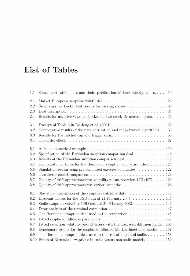
List of Tables

1.1 Some short rate models and their specification of short rate dynamics. . . . 13

2.1 Market European swaption volatilities. . . . . . . . . . . . . . . . . . . . . 23

2.2 Swap vega per bucket test results for varying strikes. . . . . . . . . . . . . 33

2.3 Deal description. . . . . . . . . . . . . . . . . . . . . . . . . . . . . . . . . 35

2.4 Results for negative vega per bucket for two-stock Bermudan option. . . . 36

3.1 Excerpt of Table 3 in De Jong et al. (2004). . . . . . . . . . . . . . . . . . 55

3.2 Comparative results of the parametrization and majorization algorithms. . 59

3.3 Results for the ratchet cap and trigger swap. . . . . . . . . . . . . . . . . . 60

3.4 The order effect. . . . . . . . . . . . . . . . . . . . . . . . . . . . . . . . . 62

5.1 A simple numerical example. . . . . . . . . . . . . . . . . . . . . . . . . . . 116

5.2 Specification of the Bermudan swaption comparison deal. . . . . . . . . . . 118

5.3 Results of the Bermudan swaption comparison deal. . . . . . . . . . . . . . 119

5.4 Computational times for the Bermudan swaption comparison deal. . . . . . 120

5.5 Simulation re-run using pre-computed exercise boundaries. . . . . . . . . . 122

5.6 Two-factor model comparison. . . . . . . . . . . . . . . . . . . . . . . . . . 123

5.7 Quality of drift approximations: volatility/mean-reversion 15%/10%. . . . 126

5.8 Quality of drift approximations: various scenarios. . . . . . . . . . . . . . . 126

6.1 Statistical description of the swaption volatility data. . . . . . . . . . . . . 145

6.2 Discount factors for the USD data of 21 February 2003. . . . . . . . . . . . 146

6.3 Smile swaption volatility USD data of 21 February 2003. . . . . . . . . . . 146

6.4 Error analysis of the terminal correlation. . . . . . . . . . . . . . . . . . . . 147

6.5 The Bermudan swaption deal used in the comparison. . . . . . . . . . . . . 148

6.6 Fitted displaced diffusion parameters. . . . . . . . . . . . . . . . . . . . . . 155

6.7 Fitted swaption volatility and fit errors with the displaced diffusion model. 155

6.8 Benchmark results for the displaced diffusion Markov-functional model. . . 157

6.9 The Bermudan swaption deal used in the test of impact of smile. . . . . . . 158

6.10 Prices of Bermudan swaptions in smile versus non-smile models. . . . . . . 159

18

xviii LIST OF TABLES

7.1 Example of a hybrid coupon swap payment structure for the floating side. . 163

7.2 Deal description for test of exact versus approximate drift in CMS models. 184

19

Notation

s A lower case italic denotes a scalar.

v A lower case bold denotes a vector.

M An upper case bold denotes a matrix.

α Day count fraction.

β Correlation parameter, see (2.4).

γ Weights; correlation parameters.

Γ Lagrange multipliers.

δ Delta: risk sensitivity with respect to

underlying rate or asset price.

∆ Tangent vector for geometric program-

ming.

ε Perturbation size; convergence criterium.

η Pay (+1)/receive (−1) fixed index; caplet

(+1)/floorlet (−1) index.

θ Drift in short rate models.

λ Largest eigenvalue of B.

Λ Diagonal eigenvalues matrix.

µ Drift.

ν Vega: risk sensitivity with respect to

volatility.

π Realized numeraire relative payoff.

ρ Target correlation, matrix form: P.

%(p,s) Performance ratio for algorithm s on

test problem p.

σ Volatility.

τi Discretization time point. Time dis-

cretization: τ1 < · · · < τm.

φ Cumulative normal distribution func-

tion; performance profile.

ϕ Objective function for rank reduction

of correlation matrices.

χ Auxiliary majorization function.

Ψ Error per-entry in correlation matrix:

Ψ = YYT −P.

ω Outcome of probability space, ω ∈ Ω.

Ω Probability space.

Sn Sphere in Rn+1.

E Expectation.

P Real-world probability measure.

Q Arbitrage-free pricing measure.

R Set of real numbers.

Sn Set of real n× n symmetric matrices.

F Filtration.

N Normal distribution.

20

xx NOTATION

O Order.

S Swap market model.

a Model parameter.

b Discount bond price; model parame-

ter.

bi Price of a discount bond maturing at

time ti.

B Helper matrix for majorization.

c Model parameter.

C Correlation matrix.

d Number of stochastic factors; the usual

d1, d2 in Black-type formulas.

e End index of a forward rate.

f Forward rate.

i(t) Spot LIBOR index at time t, see (2.3).

I Identity matrix.

k Strike rate.

m Number of discretization time points.

n Number of forward rates; numeraire

value.

o Option price.

p PVBP, present value of a basis point,

see (2.1).

P Target correlation matrix, P = (ρij)ij.

Q Orthogonal matrix, QQT = I, with I

the identity matrix.

r Short rate; instantaneous continuously

compounded interest rate.

s Swap rate; start index of a forward

rate; asset price.

t Time.

ti Tenor time. Tenor structure: 0 = t0 <

· · · < tn.

v Value of a security, asset or derivative.

w Brownian motion; weight coefficient.

Y Decomposition matrix: YYT = P,

with P a correlation matrix.

z Normally distributed random variable.

i (Subscript i) Associated with the pe-

riod [ti, ti+1] (e.g., fi, σi, αi); associ-

ated with ti (e.g, bi).

s:e (Subscript s : e) Associated with the

period [ts, te] (e.g., fs:e, σs:e).

(i+1) (Superscript (i + 1)) Associated with

the forward measure for which bi+1 is

the numeraire.

d Infinitesimal differential.

bp Basis point, 0.01%.

P&L Profit and loss.

xNCy x non-call y option, exercisable on an

underlying with a maturity of x years

from today but callable only after y

years.

· Scalar product of vectors.

21

NOTATION xxi

〈·, ·〉 Scalar product of vectors; quadratic

cross-variation.

〈·〉 Quadratic variation.

Var Variance.

Cov Covariance.

‖.‖ Vector length: Square root of sum of

squares of vector entries.

‖ · ‖F Frobenius norm, ‖Y‖2F := tr(YYT )

for matrices Y.

¿ Much smaller than.

T (Superscript T ) Matrix transpose.

22

23

Outline

The purpose of this thesis is to further knowledge of efficient valuation and risk man-

agement of interest rate derivatives (mainly of Bermudan-style but other types are also

included) by extending the theory on market models. Here, we provide an outline of the

thesis. Readers that are non-experts in the field of interest rate derivatives pricing could

skip the outline at first reading and return here after reading the introductory Chapter 1.

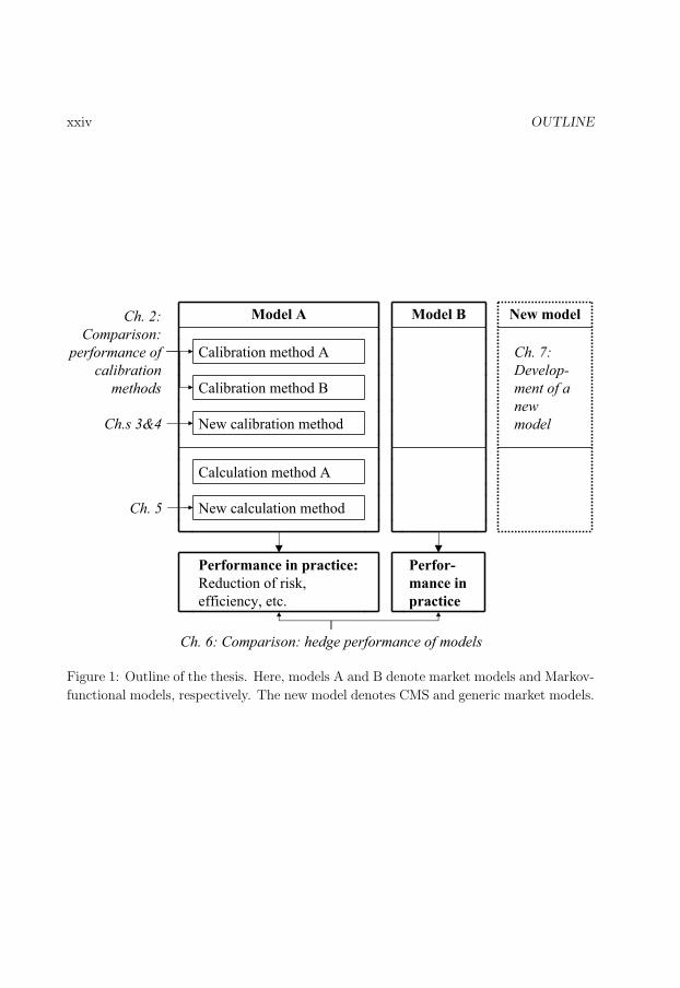
A schematic outline of the thesis is given in Figure 1.

Chapter 2 investigates various popular calibration choices for the LIBOR market model

and their effect on the quality of risk sensitivities of Bermudan swaptions. The results

show that care should be taken when selecting a calibration method: Certain choices,

e.g., so-called time-homogeneous volatility, may lead to non-efficient estimates of risk

sensitivities. Poor and unstable estimates of risk, in turn, lead to fluctuations in a hedge

portfolio that are spurious and have no economic meaning, and the risk associated with

the derivative is not adequately reduced. The results however also show that so-called

constant volatility leads to efficient and stable estimates of risk sensitivities. The combined

results are important and valuable to financial institutions that need to select a calibration

method for market models, with the aim to risk manage Bermudan swaptions and other

interest rate derivatives.

Chapter 2 has been published in the Journal of Derivatives, see Pietersz & Pelsser

(2004a). An extended abstract of the chapter has been published in Risk Magazine, see

Pietersz & Pelsser (2004b). The Risk article has been republished as part of a Risk book,

see Pietersz & Pelsser (2005b).

Chapters 3 and 4 solve the same problem in two completely different ways. The

problem is the so-called rank reduction of correlation matrices, and occurs as a key part

of calibrating multi-factor market models to correlation. Mathematically formulated, rank

reductions of correlation matrices are non-convex optimization problems, which are known

to be difficult to solve: The problem is to minimize, over low-rank correlation matrices

attainable by the model, an objective value, which is the error with the original given

correlation matrix. We present two elegant solution algorithms. The benefit over existing

algorithms is the enhanced efficiency: In terms of computational speed, the algorithms of

Chapters 3 and 4 outperform existing algorithms, in the numerical tests we considered.

24

xxiv OUTLINE

New calculation method

Calculation method A

New calibration method

Calibration method B

Calibration method A

Model A

Performance in practice:

Reduction of risk,

efficiency, etc.

Model B

Perfor-

mance in

practice

Ch. 7:

Develop-

ment of a

new

model

New model

Ch. 6: Comparison: hedge performance of models

Ch. 5

Ch.s 3&4

Ch. 2:

Comparison:

performance of

calibration

methods

Figure 1: Outline of the thesis. Here, models A and B denote market models and Markov-

functional models, respectively. The new model denotes CMS and generic market models.

25

OUTLINE xxv

Chapter 3 presents a solution for rank reduction of correlation matrices, based on

majorization, which is a general technique from optimization. We perform the task of

showing that majorization can be applied to rank reduction of correlation matrices. The

resulting algorithm is globally convergent (i.e., from any starting point) to a local mini-

mum. The algorithm is shown to be straightforward to implement, which makes its use

accessible to non-experts. The majorization algorithm is extremely efficient, because of

its low cost per iterate.

Chapter 3 has been published in Quantitative Finance, see Pietersz & Groenen (2004b).

An extended abstract of the chapter has been published in Risk Magazine, see Pietersz

& Groenen (2004a).

Chapter 4 develops a solution for rank reduction of correlation matrices based on geo-

metric programming, which is optimization over curved space (manifolds). The manifold-

equivalents of Newton and conjugate gradient optimization algorithms are presented for

the problem of rank reduction of correlation matrices. By carefully selecting the man-

ifold, we are able to bring the gradient and Hessian to natural forms, enabling an effi-

cient implementation. The geometric curved algorithms enjoy the same super-linear local

convergence properties as their Euclidean flat counterparts: Quadratic convergence for

Newton and m-steps quadratic convergence for conjugate gradient, where m denotes the

dimension of the manifold. Additionally, we develop a novel method to immediately check

whether a stationary point is a global minimum, by extending the Lagrange multiplier

results of Zhang & Wu (2003) and Wu (2003). This feature is very rare for non-convex

optimisation problems, and makes the problem of rank reduction of correlation matrices

all the more interesting. Extensive numerical tests show that geometric programming

compares favourably with other existing algorithms, in terms of computational speed.

Chapter 4 has been submitted. For the working paper version, see Grubisic & Pietersz

(2005).

Chapter 5 introduces a new discretization for the LIBOR market model, the Brow-

nian bridge discretization. Discretizations are required for implementation of a pricing

algorithm. The benefit of Brownian bridge is its accuracy when single or large time steps

are used. For single time steps, we show that it is least-squares optimal to use Brow-

nian bridge (in a to be defined natural sense). This is also confirmed in the numerical

LIBOR-in-arrears test extended from Hunter, Jackel & Joshi (2001). As a multi step dis-

cretization, we show that Brownian bridge converges weakly with order one. The multi

step convergence is illustrated by numerical tests. Finally, we show that a single time

step discretization combined with a separability assumption on the volatility, allows for

an even more efficient implementation via pricing on a grid or on a recombining lattice,

instead of Monte Carlo.

26

xxvi OUTLINE

Chapter 5 has been published in the Journal of Computational Finance, see Pietersz,

Pelsser & van Regenmortel (2004). An extended abstract has been published in Wilmott

Magazine, see Pietersz, Pelsser & van Regenmortel (2005).

Chapter 6 presents novel empirical comparisons on the performance of models in terms

of reduction of risk. The profit and loss (P&L) of hedge portfolios of Bermudan swaptions

are recorded for USD swap rates and swaptions data over a one year period. We compare

LIBOR and swap market models, and the Markov-functional model of Hunt, Kennedy

& Pelsser (2000). The Markov-functional model is representative of single-factor models,

such as short rate models. The market models are representative of multi-factor interest

rate pricing models. Both market models and Markov-functional models can be calibrated

to relevant interest rate correlations. Therefore, correlation pricing effects can be captured

in both model types. The three main conclusions of the hedge tests are quite remarkable:

First, delta hedging is compared to delta and vega hedging. Delta hedging is the-

oretically justified by the replication argument of Black & Scholes (1973) and Merton

(1973), of continuous trading in the underlying asset. Vega hedging is the offsetting of

volatility risk by trading in underlying options. Vega hedging is not based on a replica-

tion argument, and it is considered a financial engineering trick, widely applied by traders

and practitioners. We show that delta and vega hedging significantly outperforms delta

hedging, in terms of reduction of variance of P&L.

Second, the algorithm of Longstaff & Schwartz (2001) for estimating the optimal

exercise decision of American options in Monte Carlo is investigated. This algorithm is

required for market models, but not for the Markov-functional model. We show that the

algorithm contains a discontinuity, which renders convergence of finite difference estimates

of risk sensitivities to be slower, see, for example, Glasserman (2004, Section 7.1). The

hedge tests show that the less effective estimation of risk sensitivities adversely affects

reduction of variance of P&L. Moreover, we propose a novel adjustment of the Longstaff &

Schwartz (2001) algorithm, termed constant exercise decision method. With our proposed

modification, a far greater reduction of variance of P&L is attained than with the original

algorithm. The reduction is comparable to the reduction in the Markov-functional model.

Our proposal thus enables market models to function properly as risk management tools

of callable derivatives.

Third, the effect of the number of stochastic factors and correlation specification is

investigated. The hedge tests show no significant differences in terms of reduction of

variance of P&L, across: models, number of factors and correlation specification.

Finally, the effect of smile on pricing is investigated. Volatility smile is the phenomenon

that different Black (1976) implied volatilities are quoted for different strikes of otherwise

equal options. The results show that the impact of smile can be much larger than the

impact of correlation. Also, the impact of smile is similar in both market models and

Markov-functional models.

27

OUTLINE xxvii

Chapter 6 has been submitted. For a working paper version, see Pietersz & Pelsser

(2005a).

In Chapter 7, new CMS and generic market models are developed, which allow for

ease of volatility calibration for a whole new range of derivatives, such as fixed-maturity

Bermudan swaptions and Bermudan CMS swaptions. CMS and generic market mod-

els allow for a choice of forward rates other than the classical LIBOR and swap rates

in the LIBOR and swap market models, respectively. We present a theoretical result

with necessary and sufficient conditions for an arbitrary structure of forward rates to be

arbitrage-free at all possible states of the model. CMS and generic drift terms for the

forward rates are derived, by use of matrix notation, for both terminal and spot measures.

A fast algorithm is presented that approximately, but accurately, calculates forward rates

over time steps for CMS market models.

Chapter 7 has been submitted. For a working paper version, see Pietersz & van

Regenmortel (2005).

28

29

Chapter 1

Introduction

Bermudan-style interest rate derivatives are an important class of options. Many banking

and insurance products, such as mortgages, cancellable bonds, and life insurance products,

contain Bermudan interest rate options associated with early redemption or cancellation

of the contract. The abundance of these options makes evident that their proper valuation

and risk measurement are important to banks and insurance companies. Risk measure-

ment allows for offsetting market risk by hedging with underlying liquidly traded assets

and options.

The purpose of this thesis is to further knowledge of efficient valuation and risk man-

agement of Bermudan-style interest rate derivatives. In this chapter, we provide a historic

background and comprehensive framework for the chapters that are to follow.

The outline of this chapter is as follows. First, we introduce the use of models for

arbitrage-free pricing. Second, we briefly describe interest rate markets and options.

Third, we provide an overview of interest rate derivatives pricing models relevant to the

thesis. Fourth, American option pricing with Monte Carlo simulation is discussed.

1.1 Arbitrage-free pricing

In this thesis, pricing models produce relative valuations. The relative valuation of an

asset (most often a derivative) is in terms of other asset prices. Pricing models are thus

viewed as an ‘extrapolation tool’ that aim to extrapolate derivative prices from underlying

assets.

Key to relative valuation models is the exclusion of arbitrage. An arbitrage is an

opportunity to make a risk-less profit with positive probability, with no costs at time

of execution. If an arbitrage opportunity occurs, then many investors buy the arbitrage

opportunity, driving up the arbitrage price. Eventually, this causes the arbitrage to

30

2 CHAPTER 1. INTRODUCTION

disappear. Arbitrage opportunities are therefore not likely to occur in an efficient and

competitive economy.

When we construct a relative valuation model, then we usually do so by specifying

dynamics of certain base asset prices in a frictionless arbitrage-free market. We then

consider, for example, derivatives whose values derive from these base assets. A self-

financing portfolio is a portfolio without injection or withdrawal of funds. A derivative

that we added to the model is said to be attainable if its payoff can be exactly replicated

by a dynamically managed self-financing portfolio of the base assets. We call a model

complete if all the derivatives that we added to the model are attainable. In a complete

model, any added derivative is effectively redundant (in this theoretical world), since it

is merely a particular dynamic portfolio of the base assets. The added derivatives are

said to be spanned by the underlying assets. In a complete model, any derivative price

is already known when the current underlying prices and their dynamics are known: The

current derivative price is simply equal to the current value of a replicating portfolio.

Next to absence of arbitrage, we also assume absence of transaction costs : there is

no difference in price when buying or selling an asset. This assumption obviously does

not reflect reality. In the presence of transaction costs, arbitrageurs cannot exploit all

theoretical arbitrage opportunities, since transaction costs make some of these no longer

profitable. However, for large market participants, transaction costs are sufficiently low

relative to transaction sizes. In effect, the assumption of zero transaction costs is quite

accurate for the market as a whole. Moreover, the assumption of absence of transaction

costs leads to a theory that is still sufficiently accurate, but much more tractable.

Model dynamics of returns on asset prices, in the real-world measure, consist of two

parts: An average part (drift) and a random part (diffusion). The diffusion part can be

modelled as either continuous (e.g., Brownian motion) or discontinuous (e.g., jumps as in

Merton (1976)). The use of continuous diffusion models is widespread, foremost because

continuous models provide a more than sufficiently accurate description of reality, and

also because of analytical tractability. This thesis therefore considers only continuous

diffusion models. If it is then assumed that asset returns over disjoint time periods are

independent, then it follows from the Levy-Khinchin theorem that the diffusion term is a

(time- and state-dependent) volatility coefficient times a Brownian motion.

We summarize these concepts in terms of stochastic differential equations (SDEs). We

consider a model with a filtered probability space (Ω,P,F) with filtration F = (F(t))t≥0,

on which is defined a F -adapted Brownian motion w. Here, P denotes the real-world

measure. The asset price is denoted by s, its F -adapted drift by µ and its F -adapted

volatility by σ. A realization in Ω is denoted by ω. We have:

ds(t)

s(t)= µ(t, ω)dt + σ(t, ω)dw(t).

31

1.1. ARBITRAGE-FREE PRICING 3

Also, we assume the existence of a money market account with price b and return r(t, ω):

db(t)

b(t)= r(t, ω)dt.

The market price of risk (or Sharpe ratio, see Sharpe (1964)) is defined to be the

excess average return over the risk free rate divided by the volatility of the asset. In other

words, it is (drift-[risk free rate])/volatility and (µ − r)/σ, see, e.g., Baxter & Rennie

(1996, page 119). A sufficient condition for no-arbitrage is equality of market prices of

risk for all assets, e.g., Hull (2000, Equation (19.6)). The actual levels of market prices of

risk then turn out not to matter for valuation.

We introduce some key concepts of arbitrage-free pricing. A numeraire is an asset

with a strictly positive value at all times. Asset prices may be denominated in terms

of amounts of the numeraire. A martingale is a process with zero drift. Suppose we

can construct a new measure (the so-called risk neutral measure) such that all numeraire-

expressed asset prices become martingales. It can be shown (e.g., Hunt & Kennedy (2000,

Theorem 7.32)) that the assumption of existence of such a measure automatically implies

that the model is arbitrage-free. Moreover, if there exists a single unique risk neutral

measure, then it can be shown (e.g., Hunt & Kennedy (2000, Theorem 7.41)) that the

model is complete, i.e., every derivative security is attainable by a replicating portfolio in

the underlying assets.

Given the assumption of equality of all market prices of risk, we may apply Girsanov’s

theorem (e.g., Øksendal (1998, Theorem 8.6.4)) to construct the risk-neutral measure.

Under the risk neutral measure, market prices of risk then turn out to disappear. Therefore

these do not affect arbitrage-free pricing.

The martingale property of numeraire-relative asset prices implies that their future

expectations take today’s value. If s and n denote prices of an asset and a numeraire,

respectively, thens(0)

n(0)= E

[s(t)

n(t)

], for t ≥ 0.

where the expectation is with respect to the risk-neutral measure. The price v of a

derivative (also an asset), necessarily sharing the same market price of risk, then satisfies

v(0) = n(0)E[v(t)

n(t)

], for t ≥ 0, (1.1)

which is the fundamental arbitrage-free pricing formula, see, e.g., Bjork (2004, Theorem

10.18). We note that the market price of risk does not occur in this formula. If we calculate

(1.1) for a call option on a stock that is modelled as geometric Brownian motion, then we

obtain the famous formula of Black & Scholes (1973).

32


In practice, we directly model under a risk-neutral measure, by specifying the part

that stems from the real-world measure, the diffusion part. No-arbitrage requirements

then fully fix the drift term. In fact, for European call and put options, traders quote

the diffusion part: so-called implied volatility. It is the volatility to be used in the Black-

Scholes formula to obtain the European option price. A European option is an option

that is exercisable only at a single point in time (usually during a single trading day).

The reason that the derivative price is fully fixed by (1.1) is replication by a self-

financing portfolio. Suppose amounts δs of s and δb of b are held, then the value v is given

by:

v = sδs + bδb, (1.2)

The change in value v of a self-financing portfolio thus satisfies (e.g, Joshi (2003a, Equa-

tions (5.58) and (5.59))):

dv = δsds + δbdb. (1.3)

In other words, value changes due to trading in the asset s and risk-free asset b cancel

exactly:

sdδs + bdδb = 0.

A replicating portfolio is a dynamically managed self-financing portfolio of underlying

assets s and b, which has a value equal to the payoff of derivative v, in all possible future

states of the economy.

The replicating portfolio holds a dynamic amount of δs of the underlying asset s. The

amount δs can be calculated from (1.2), (1.3), and from Ito’s formula: If s is a stochastic

process, and v : R→ R is a function, then for the process v(s) we have:

dv =∂v

∂sds +

1

2

∂2v

∂s2d〈s〉, (1.4)

see, for example, Karatzas & Shreve (1991, Theorem 3.3.3). Here, angle brackets 〈·〉denote quadratic variation, see, e.g., Øksendal (1998, Exercise 2.17). By rewriting (1.4)

in the form of (1.3), we can show that

δs =∂v

∂s. (1.5)

The quantity δs is called the delta, and it is an example of a risk sensitivity : the risk

sensitivity with respect to the underlying asset price.

1.1.1 Use of models in practice

A dynamic hedge of the derivative v consists of taking an opposite position in the repli-

cating portfolio. In practice, the hedge is not re-balanced on a continuous basis, rather at

33

1.1. ARBITRAGE-FREE PRICING 5

discrete points in time. Re-balancing usually takes place when delta risk exceeds a cer-

tain threshold level. The adaption from continuous-time to discrete-time hedging works

extremely well in practice, and forms the basis for the success of arbitrage-free pricing

models.

While we use risk-neutral pricing models as relative valuation and hedging tools, it is

interesting to note that these models also make assertions on real-world price dynamics,

through the connection with the real-world measure. Risk-neutral models can thus also

be viewed as economic models, attempting to model economic reality. Though modelling

of real-world price dynamics is a vital aspect of risk-neutral models, it is not the most

important aspect. More important to risk-neutral models are:

1. To produce sensible prices of derivatives, and to reproduce prices of underlying

assets and options exactly.

2. To adequately reduce variance of profit and loss (P&L), when a hedge is set up.

3. To efficiently produce prices, i.e., within a limited amount of computational time.

The difference between the use of a model as a hedging tool or economic model has

important implications. For example, consider modelling the term structure of interest

rates. Extensive empirical research has shown that the term structure is driven by more

than one stochastic factors, see the review article of Dai & Singleton (2003). For an

economic model, we should thus use at least two factors, and a single-factor model is

simply not acceptable. However, for a model used as hedging tool, it is perfectly sensible

to consider a single-factor model, as long as it satisfies the above three properties.

The necessity that pricing models need reproduce prices of underlying assets and

options has two further implications:

First, option price data (implied volatility) determines the diffusion part (or, equiv-

alently, volatility) of the model, rather than time-series estimates from historic data on

asset returns. The reason is straightforward: Certain features of a derivative may become

redundant during the life of the derivative, which may render the derivative equivalent to

(or almost equivalent to) a market traded option. In that case, the model should produce

a derivative price equal to the market traded option price, otherwise the financial institu-

tion holding the derivative can incur arbitrage, which should be avoided. The only way

to avoid arbitrage is to make the model consistent with prices of underlying options, i.e.,

to use implied volatility for the diffusion term in the model. The process of making the

model consistent with market prices is called calibration.

Second, a pricing model is re-calibrated to the most recent implied volatility data,

whenever the derivative needs be valued. The important reason is again that of no-

arbitrage, and is the same as above for the use of implied volatility in models. Implied

34


volatility quotes change over time. The practice of re-calibration to unpredictably chang-

ing volatility is not consistent with most pricing models (excluding stochastic volatility

models), since most models assume volatility to be known over the model time horizon.

When implied volatility changes, then a derivative value may change too, due to the

practice of re-calibration. As a result, derivative traders face volatility risk (vega). The

risk may be offset by vega hedging. If σ denotes the volatility, and o the price of an

underlying option, then the following portfolio has zero volatility risk (for small changes

in σ):

one derivative (v) and − ∂v/∂σ

∂o/∂σoptions (o). (1.6)

A delta hedge with the underlying asset as in (1.5) can then be applied to the vega-neutral

portfolio in (1.6).

Vega hedging is out-of-model hedging, since we hedge parameters that are input to

the model. Delta hedging with the underlying asset in (1.5) is in-model hedging, since

the underlying asset price is a state variable of the model. Nonetheless, vega hedging

is not inconsistent with arbitrage-free pricing models: We are only holding a different

portfolio of derivatives and options that needs to be delta hedged. From an arbitrage-free

pricing perspective though, there is simply no need to add the additional options (though

such addition is allowed): the original derivative is already perfectly delta-replicable in

the theoretical model world. In practice however, vega hedging enables a significant

additional reduction of variance of P&L, and it thus contributes to wealth preservation.

Another practice for arbitrage-free pricing models is that of customizing a model to a

certain product. We construct the model in such way that all parts of economic reality,

relevant to the product, are incorporated into the model. The benefit is that the product

is priced correctly, while not having to fully model all parts of the market, thereby often

attaining a more efficient implementation.

1.2 Interest rate markets and options

In interest rate markets, participants trade primarily in interest rate agreements. An

interest rate agreement is an agreement to borrow or lend money, over an agreed period

of time, against agreed periodical payments (interest rate payments) that are in some

form denoted as a percentage (interest rate) of the underlying borrowed or lent amount

(notional amount).

We refer to the length of an interest rate agreement as its tenor. Different tenors may

attract different interest rates, which gives rise to the so-called term structure of interest

rates.

35

1.2. INTEREST RATE MARKETS AND OPTIONS 7

The above description of an interest rate agreement includes money market deposits,

bonds, forward interest rate agreements, and swaps. Money market deposits, bonds, and

swaps are of particular relevance to this thesis, therefore we explain their workings in

some detail.

1.2.1 Linear products: Deposits, bonds, and swaps

Money market deposits usually have a maturity of one year or less. The two parties

agree on an interest rate and one party deposits the notional amount. At the end of

the agreement (at maturity), the other party returns the notional and makes the agreed

interest rate payments.

A bond is an agreement between two parties, the borrower and the lender, on a

designated notional amount. At initiation, the borrower receives a pre-negotiated amount

for the bond (not necessarily equal to the notional amount). During the life of the bond,

the borrower makes coupon payments on the notional amount, usually on the basis of a

fixed contractually agreed rate, but the coupon payments could also be based on a floating

interest rate. By a floating interest rate, we mean the prevailing market interest rate for

the tenor spacing between the floating interest rate payments. We discuss the method for

determining this floating interest rate below. If there are no coupon payments during the

life of the bond, then we call such a bond a zero coupon bond. At maturity of a bond, the

borrower returns the notional amount to the lender.

Interest rate swaps typically have a maturity of two years or more. Interest rate swaps

involve only exchanges of interest rate payments, but normally do not involve exchanges

of notional. The two parties agree on an interest rate. Periodically, one party pays this

agreed interest rate (the fixed rate), while the other party pays a floating interest rate. We

remark that the frequency of fixed and floating payments may differ. Typical frequencies

are annually, semi-annually, quarterly, and monthly.

The fixed rate at which market participants can enter into a swap agreement at other-

wise zero cost is called the swap rate. Swap rates can be seen as long term borrowing and

lending rates. In fact, the swap rate for a swap with a particular tenor is more or less the

interest rate for that particular tenor. The reason is that a swap can be used to create a

synthetic borrowing or lending agreement at a single interest rate over the tenor period

of the swap: Suppose we borrow money through deposits with floating interest rates, and

we enter into a swap in which we pay fixed, on a notional equal to the amount borrowed

from the deposit. At the end of each deposit, we borrow the same amount again in the

deposit market, in order to pay back the notional from the previous deposit agreement.

Rolling over money market deposits in such way, the resulting deposit interest payments

cancel against the floating interest we receive from the swap; the fixed swap payments

remain. Effectively, we then pay a fixed interest rate on our loan over the life of the swap.

36


The two parties in a swap determine the floating interest rate usually via a reference

interest rate. Reference rates are used to calculate payments not only of swaps, but also

of other securities, such as interest rate derivatives. A reference interest rate is a rate

that is set by a financial authority or calculation agent. Examples are:

LIBOR: London inter-bank offered rate, published by the British Bankers’ Association

(BBA), each trading day at noon (12.00am) London time.

EURIBOR: Euro inter-bank offered rate, published by the European Banking Federation

(FBE) and by the Financial Markets Association (ACI), each trading day at around

11.00am central European time.

These reference rates are published for several tenors and currencies. Upon publication

of the reference rate, practitioners say that the rate then fixes.

Financial authorities determine reference rates normally along the following lines: A

number of panel banks are consulted. Each panel bank provides rates at which it conceives

it possible to borrow money in the inter-bank market, for various tenors and currencies.

For each tenor and currency, some percentile of the top and bottom of the quotes are

discarded. The remaining quotes are averaged to form the reference rate for that tenor

and currency. It is interesting to note there is now an interest rate derivatives pricing

model that bears the name of a reference rate: the LIBOR market model, see Section 1.3.

An interesting note is that the first major swap took place only in 1981, between IBM

and the World Bank, see Valdez (1997, pages 269–270).

1.2.2 Interest rate options: Caps, floors, and swaptions

The plain-vanilla European interest rate options most relevant to this thesis are (i) caps

and floors, and, (ii) swaptions. A cap consists of a sequence of consecutive caplets, and,

likewise, a floor consists of a sequence of consecutive floorlets. Caplets and floorlets are

call and put options, respectively, on LIBOR rates. Swaptions are options on swap rates.

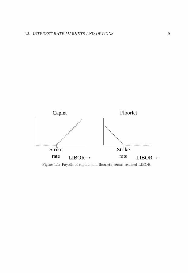
A caplet (respectively, a floorlet) gives its holder at expiry the right, but not the

obligation, to enter into a borrowing deposit (lending deposit) at a pre-arranged strike

rate. If an option holder claims the option right, then we say that he or she exercises

the option. If LIBOR fixes below (above) the respective strike rate, then it is cheaper to

borrow (more rewarding to lend) in the market; whereby it is sensible not to exercise the

caplet (floorlet) and it ends worthless. If LIBOR fixes above (below) the respective strike

rate, then it is sensible to exercise the caplet (floorlet), since we then receive the positive

difference LIBOR minus strike (strike minus LIBOR) at the deposit payment date. The

option gains at the deposit payment date as dependent on realized LIBOR are displayed

in Figure 1.1.

37

1.2. INTEREST RATE MARKETS AND OPTIONS 9

Strikerate LIBOR→

Strikerate LIBOR→

Caplet Floorlet

Figure 1.1: Payoffs of caplets and floorlets versus realized LIBOR.

38


A European swaption gives its holder at expiry the right, but not the obligation, to

enter into a swap with a fixed rate equal to a pre-arranged strike rate. Market participants

invariably indicate the direction of swap cash flows from the point of view of whether fixed

payments are payed or received. Thus, if we hold a swaption that gives us the right to

enter into a swap for which we pay or receive fixed, then such a swaption is a payer or

receiver swaption, respectively. A payer (respectively, a receiver) swaption corresponds

to a call option (put option). The payoff structures for payer and receiver swaptions are

similar to those of caplets and floorlets in Figure 1.1: instead of ‘LIBOR’ read ‘swap rate’,

and instead of ‘caplet’ or ‘floorlet’ read ‘payer swaption’ or ‘receiver swaption’.

Cash settled contracts differ from normal option contracts, in that they pay the relevant

difference between realized rate and strike, if this is positive. For a cash settled swaption

at expiry, both parties need to agree on ‘the’ swap rate manifest in the market. Usually,

again a reference rate is used. An example of a reference swap rate is ISDAFIX, published

for various tenors and currencies by the International Swaps and Derivatives Association

(ISDA). Financial authorities calculate swap reference rates more or less in the same way

as deposit reference rates are set; via consultation of a group of panel banks.

From Figure 1.1, we find that an option always provides a nonnegative cash flow, with a

positive probability to provide a positive cash flow, therefore we require a positive premium

for the option. To calculate cap and floor or swaption premiums, market participants

initially used a Black-type formula that is based on assuming a log-normal distribution for

the LIBOR or swap rate at expiry. This approach however lacked a theoretical justification

for long, but the approach later turned out to be valid. Moreover, an assumption of

jointly log-normal LIBOR and swap rates is inconsistent. Many researchers therefore

considered the use of the Black formula for caps and floors or swaptions to be unsound

for a considerable period: While the Black swaptions approach had already been justified

in 1990, articles establishing its validity kept appearing at least until 1997, see Rebonato

(2004a, Section 4(d)).

We present the Black approach for caps and floors; the approach is similar for swap-

tions. Prior to that, we introduce some terminology: We set out by specifying a tenor

structure, 0 = t0 < t1 < · · · < tn+1. Let αi denote the day count fraction for the period

[ti, ti+1]. A discount bond is a hypothetical security that pays one unit of currency at its

maturity, and has no other cash flows. The time-t price of a discount bond with maturity

ti is denoted by bi(t).

To present the Black approach for caps and floors, we consider two tenor points 0 <

t1 < t2. LIBOR fixes at time t1 and interest is paid at time t2. We define the forward

LIBOR rate f1(t) by

f1(t) =b1(t)− b2(t)

α1b2(t). (1.7)

39

1.3. INTEREST RATE DERIVATIVES PRICING MODELS 11

We consider the forward measure, which is the measure associated with the discount bond

b2 maturing at the payment date of the LIBOR deposit. By the assumption of absence

of arbitrage, it follows that f1 is a martingale under its forward measure. To see this,

note that f1(t) in (1.7) is the value of a portfolio ((b1(t) − b2(t))/α1) expressed in terms

of amounts of the numeraire b2(t).

Continuing, we assume that the forward LIBOR rate is a log-normal martingale under

its forward measure:

df1(t)

f1(t)= σ1dw(t), equivalently, f1(t) = f1(0) exp

(− 1

2σ2

1t + σ1w(t)

), (1.8)

where σ1 is a scalar constant. The payoff v(t2) at time t2 of a caplet with strike rate k is

then given by α1 max(f1(t1)− k, 0). From (1.1), we find for the caplet value v(0):

v(0) = n(0)E[v(t2)

n(t2)

]= b2(0)E

[α1 max(f1(t1)− k, 0)

b2(t2)

]

(∗)= α1b2(0)E

[max(f1(t1)− k, 0)

]. (1.9)

Equality (∗) holds since b2(t2) = 1. If we calculate (1.9) in full, we obtain the formula of

Black (1976):

v(0) = α1b2(0)η

f1(0)φ(ηd1

)− kφ(ηd2

),

d1,2 =ln

(f1(0)

k

)± 1

2σ2

1t1

σ1

√t1

.

Here, η denotes +1 for a caplet, and −1 for a floorlet; φ(·) denotes the cumulative normal

distribution function.

1.3 Interest rate derivatives pricing models

Up to here we have examined options on a single interest rate, such as caps, floors and

European swaptions. There are however many interesting interest rate derivatives that

depend not only on a single interest rate, but on multiple interest rates. Examples in-

clude Bermudan-style interest rate derivatives. Bermudan means that the derivative is

exercisable (equivalently: callable) at multiple discrete time points, usually separated by,

e.g., annual or semi-annual periods.

Exercise of a Bermudan derivative is a trade-off between taking the option gains now

or holding onto the option at possibly more favourable option gains later. Inherently,

values of Bermudan interest rate derivatives therefore depend on multiple interest rates.

There are of course also many non-Bermudan interest rate derivatives that dependent on

40


multiple interest rates. To value such multi-rate dependent products, we need a model

that features dynamics for the whole term structure of interest rates. Preferably, such

dynamic term structure models need be consistent with the Black formula for caps, floors

and swaptions.

1.3.1 Short rate models

Historically, the first dynamic term structure models are short rate models. The short

rate r is a hypothetical rate: it is the instantaneous rate of interest for the floating money

market account (equivalently: bank account) with value n:

dn

n= rdt, equivalently, n(t) = n(0) exp

( ∫ t

0

r(s)ds

).

In a short rate model, we select the bank account as numeraire. Discount bond prices

satisfy, by the fundamental arbitrage-free pricing formula (1.1):

bi(t, r) = E[

bi

(ti, r(ti)

)︸︷︷︸

=1

n(t)

n(ti)

∣∣∣∣r(t) = r

]= E

[exp

(−

∫ ti

t

r(s)ds

)∣∣∣∣r(t) = r

], for t < ti.

(1.10)

From (1.10), we can calculate discount bond prices, once the arbitrage-free dynamics of

the short rate are known. For most main-stream short rate models, we can find explicit

and analytical formulas for (1.10) for discount bond prices given the associated short rate.

Short rate models are characterized by their specification of dynamics for the short rate.

Examples of short rate models are given in Table 1.1 (this table is not complete).

As can be seen from Table 1.1, there are many short rate models. Next to short rate

models, there are many more other interest rate derivatives pricing models. The reason for

this abundance of interest rate models stems from different specifications of the interest

rate market, as explained below.

To specify discount bond price dynamics, we need only specify the volatility term σ(b)i ,

the drift term then follows from no-arbitrage restrictions, as explained in Section 1.1.

Therefore, we omit the drift, and focus on the diffusion term:

dbi

bi

= · · ·+ σ(b)i (t, ω)dw(t). (1.11)

The bond price volatility may thus be state-dependent.

A set of discount bond prices may be alternatively given by a set of interest rates. For

example, discount bond prices may be given (implicitly or explicitly) in terms of a set of

forward LIBOR rates f = (f1, . . . , fn):

1 + αifi =bi

bi+1

, (1.12)

41


Table 1.1: Some short rate models and their specification of short rate dynamics. Here,

the scalars a, b, and c denote model parameters.

Model Specification

Merton (1973) dr = bdt + σdw

Vasicek (1977) dr = (b− ar)dt + σdw

Dothan (1978) dr = ardt + σrdw

Brennan & Schwartz (1979) dr = (b− ar)dt + σrdw

Cox, Ingersoll & Ross (1985) dr = (b− ar)dt + σ√

rdw

Ho & Lee (1986) dr = θ(t)dt + σdw

Hull & White (1990) dr = (θ(t)− ar)dt + σdw

dr = (θ(t)− ar)dt + σ√

rdw

Black, Derman & Toy (1990) dr = θ(t)rdt + σrdw

Black & Karasinski (1991) dr = (ar − br log r)dt + σrdw

Pearson & Sun (1994) dr = (b− ar)dt + σ√

r − c dw

or in terms of the short rate r, see (1.10). Dynamics for a set of forward LIBOR rates or

for the short rate give rise to dynamics for discount bond prices, and vice versa. In fact, it

is the requirement of deterministic and known volatility for an interest rate specification

that determines a model. Thus, if we require volatility to be only time dependent σ(t),

and not state dependent, for one of the specifications, then we obtain stochastic volatility

for the other specifications:

dbi

bi

= · · ·+ σ(b)i (t) dw(t) ⇒

drr

= · · ·+ σ(r)(t, ω) dw(t)

dfi

fi= · · ·+ σ

(f)i (t, ω) dw(t)

(1.13)

dr

r= · · ·+ σ(r)(t) dw(t) ⇒

dfi

fi= · · ·+ σ

(f)i (t, ω) dw(t)

dbi

bi= · · ·+ σ

(b)i (t, ω) dw(t)

(1.14)

dfi

fi

= · · ·+ σ(f)i (t) dw(t) ⇒

dbi

bi= · · ·+ σ

(b)i (t, ω) dw(t)

drr

= · · ·+ σ(r)(t, ω) dw(t)(1.15)

Specification (1.13) corresponds to the extension of Black & Scholes (1973) from stocks

to bonds, (1.14) corresponds to short rate models, and (1.15) to the LIBOR market model.

We restrict our exposition to these model classes. More specifications are available: in

fact, Rebonato (2004a, Section 3) lists five specifications.

42


Bond options can be viewed as caplets and floorlets, see Hull (2000, Equation 20.10).

The straight extension of the model of Black & Scholes (1973) from stocks to bonds, i.e.,

deterministic and known instantaneous bond volatility, suffers however from the problem

that discount bond prices do not necessarily converge to one at maturity. There are also

other related problems, see Rebonato (2004a, Section 4(b)). Therefore a direct application

of Black & Scholes (1973) to bond prices yields an interest rate derivatives pricing model

with many undesirable features.

The initial success of short rate models is mainly due to their analytical tractability

and numerical efficiency. There are, however, also some drawbacks to short rate models:

They are, in a sense, difficult to calibrate, as model parameters need be implied from mar-

ket option prices via non-straightforward numerical procedures. The resulting numerical

calibration procedures can be instable and computationally costly. The reason is that

short rate models are formulated in terms of an artificial short rate that is not directly

observable in the market. Moreover, deterministic volatility for an abstract short rate in

(1.14) does not correspond to market practice of quoting implied volatility for LIBOR

and swap rates, see Section 1.2. Consequently, model parameters need to be tweaked to

ensure the model fits to the relevant market rates and volatilities.

An example of the indirect calibration of short rate models is when they are calibrated

to swaption volatility: we then have to resort to the formula of Jamshidian (1989): A

swaption is viewed as an option on a coupon paying bond. Jamshidian (1989) decomposes

the option on the coupon paying bond into several options on discount bonds.

Another disadvantageous feature of short rate models is that they produce an arbitrary

volatility smile. Volatility smile is the phenomenon that different implied volatility is

quoted for options that have different strikes but that are otherwise identical. The classical

model of Black & Scholes (1973) exhibits a so-called flat volatility smile, in the sense that

the implied volatility is independent of strike. We thus expect from any interest rate

model that aims to be the equivalent of Black & Scholes (1973) for interest rates to also

produce a flat volatility smile. Such is, as stated before, not the case for short rate models.

Smile volatility is more realistic than flat volatility, since we can observe a pronounced

volatility smile in interest rate markets. However, the produced smile ought to correspond

also qualitatively to the observed smile, and such is not the case for short rate models:

the latter exhibit rather arbitrary smiles, and smile shapes are not controllable by model

users, at least not without further modification.

Typically, short rate models have only a single stochastic driver, although some two

factor short rate models exist too, see, for example, Longstaff & Schwartz (1992) and

Ritchken & Sankarasubramanian (1995). An advantage of single factor models is that

recombining lattices can be used to efficiently price mildly path-dependent derivatives,

including American-type options. A disadvantage is the resulting difficulty to model

instantaneous de-correlation.

43


For a more extensive discussion on advantages and disadvantages of short rate models

(e.g., positivity of interest rates and non-explosiveness of short rate models), the reader

is referred to Cairns (2004, Section 4.1).

1.3.2 Market models

In recent years, a successful class of models has appeared in the literature known as market

models (LIBOR and swap market models, also referred to as BGM models, see Brace,

Gatarek & Musiela (1997), Miltersen, Sandmann & Sondermann (1997) and Jamshidian

(1997)) or string models (see Santa-Clara & Sornette (2001) and Longstaff, Santa-Clara &

Schwartz (2001)). Kerkhof & Pelsser (2002) show that the two formulations are equivalent.

Market models correspond to specification (1.15). For an arbitrage-free construction of

the LIBOR market model starting from discount bond dynamics (1.11), see Pietersz (2001,

Section 3.2). It is specification (1.15) with which traders quote prices of underlying options

(caps and swaptions). Market models therefore allow for straightforward calibration to

prices of underlying options: the model parameter is simply equal to the market quoted

volatility.

Market models are based on the forward measure technique for caplets, presented in

Section 1.2. Moreover, market models are the equivalent of Black & Scholes (1973) for

interest rates, because the LIBOR and swap market model produce flat volatility for caps

and swaptions, respectively. Positivity of interest rates is guaranteed for the deterministic

volatility LIBOR market model, since forward LIBOR rates are log-normal martingales.

In LIBOR market models, forward swap rates are generally not log-normally dis-

tributed. This seems to imply that the LIBOR market model produces non-flat swaption

volatility, and is thus not a canonical model for swaptions. Such deviation from the log-

normal paradigm however turns out to be extremely small in the LIBOR market model,

see Chapter 2.5. Fortunately for the LIBOR market model, there also exist extremely

accurate approximate formulas for swaption implied volatility. Consequently, the LIBOR

market model can be calibrated to swaption volatility. This joint cap-swaption calibration

potential of the LIBOR market model has very much contributed to its success. An inter-

esting use of the approximate swaption volatility calibration via semidefinite programming

is given in Brace & Womersley (2000) and D’Aspremont (2003).

The ease of calibration of market models allows for modelling of other market aspects,

such as time homogeneity of cap and swaption volatility. Time homogeneity of volatil-

ity means that the model preserves the cap or swaption volatility curves as model-time

progresses. In Chapter 2, we investigate the effect of including such time homogeneous

calibration procedures on the quality of risk sensitivities produced by the model.

Market models correspond to (1.15), and are thus based on a set of forward rates.

These forward rates are, in fact, the state variables of the model. The number of state

44


variables can grow large for particular trades: For a thirty years model with semi-annual

forward rates, the model has sixty forward rates. This means that market models have

large dimensionality. We address reduction of dimensionality in Chapters 3 and 4.

Due to the dimensionality of market models, Monte Carlo simulation has to be used to

value derivatives, which is non-efficient compared to recombining lattices used in short rate

models. Technological computer hardware developments have however recently enabled

the use of Monte Carlo as a sufficiently efficient pricing and risk management tool. In

Chapter 5, we study an efficient and accurate approximation of the LIBOR market model

that enables pricing on a recombining lattice.

Though some derivatives can be valued without Monte Carlo when a short rate or

Markov-functional model is used, the trend shows a growing complexity in derivatives.

Certain derivatives have become so complex and strongly path-dependent, that these can

only be valued with Monte Carlo anyway, whether a low factor (short rate or Markov-

functional) or multi factor model is used.

Volatility smile can be incorporated in the LIBOR market model, see, for example,

Andersen & Andreasen (2000).

The traditional LIBOR market model is based on a set of forward LIBOR rates.

Jamshidian (1997) extends the market model technology to a set of forward swap rates

that co-end at the same final date. Hunt & Kennedy (2000, Section 18.4) and Galluccio &

Hunter (2004) extend with a set of forward swap rates that co-start at the same initial date,

which is useful for, e.g., European options on interest rate spreads. An interest rate spread

is a difference between separate interest rates. In Chapter 7, we extend market models

to include forward constant maturity swap (CMS) rates and other generic specifications

of rates. The derivation methodology is fully generic and includes the previous market

model specifications. The CMS market model is key to the pricing of, for example, fixed

maturity Bermudan swaptions and Bermudan CMS swaptions.

1.3.3 Markov-functional models

A model class that combines some of the features of short rate models and market models

is the Markov-functional model of Hunt et al. (2000), see also Hunt & Kennedy (2000,

Section 19) and Pelsser (2000, Section 9). Markov-functional models can be calibrated

to interest rate option volatility much like market models, and they do not suffer from

the drawback of short rate models of producing an arbitrary smile: Volatility smile is

very much controllable in Markov-functional models, and a flat volatility smile can be

achieved. Moreover, Markov-functional models do not suffer from the computational

burden of market models, and pricing can be efficiently performed on, e.g., a grid.

The numerical efficiency of pricing on a grid comes however with a price: a single

stochastic Markov driver implies that the model has difficulty in attaining instantaneous

45

1.4. AMERICAN OPTION PRICING WITH MONTE CARLO SIMULATION 17

de-correlation between interest rates. A question that has not yet been addressed in the

academic literature so far, is whether a lack of de-correlation causes a significant impact

on the pricing and hedge performance of a model. In Chapter 6, we address this research

question by empirical comparison of market models and Markov-functional models, in

terms of pricing and hedge performance.

1.4 American option pricing with Monte Carlo sim-

ulation

American options feature a period during which the option can be exercised. Bermudan

options can be exercised at several discrete points in time. Bermudan options are thus

somewhat in between European and American options.

The valuation of American options typically involves a backward induction routine,

while Monte Carlo simulation is of forward induction type. An efficient algorithm for

pricing American options in Monte Carlo was therefore not known in the literature for

long. The problem is that we need to know, at a simulation node, the value of holding

onto the option. This conditional expectation value is not known, and to calculate it

would, in principle, require simulation within simulation, which is most inefficient. Only

recently has efficient American option valuation with Monte Carlo been enabled by novel

regression-based methods, see, for example, Longstaff & Schwartz (2001). The key is

to make use of cross-sectional information present in the simulation, by regressing the

hold-on value onto functions of explanatory variables present in the simulation. The

regression-based approximate hold-on value may then be used to formulate an exercise

decision.

The regression based techniques have been generalized to stochastic mesh methods

by Broadie & Glasserman (2004) and Avramidis & Matzinger (2004). Other American

option pricing techniques include the dual approach of Rogers (2002), see also Jamshidian

(2003), and the high-dimensional grid approach of Berridge & Schumacher (2003).

In Chapter 6, we show that the regression-based algorithm of Longstaff & Schwartz

(2001) leads to inefficiently estimated risk sensitivities. We propose a modification of

the algorithm, deemed the constant exercise method, that enhances the quality of risk

sensitivity estimates.

46

47

Chapter 2

Risk-managing Bermudan swaptions

in a LIBOR model

1 This chapter presents a new approach to calculating swap vega per bucket in a LIBOR

model. It shows that for some forms of volatility an approach based on recalibration may

make estimated swap vega very uncertain, as the instantaneous volatility structure may

be distorted by recalibration. This does not happen in the case of constant swap rate

volatility.

An alternative approach not based on recalibration comes out of comparison with

the swap market model. It accurately estimates vegas for any volatility function in few

simulation paths. The key to the method is that the perturbation in LIBOR volatility

is distributed in a clear, stable, and well-understood fashion, while in the recalibration

method the change in volatility is hidden and potentially unstable.

2.1 Introduction

The LIBOR interest rate model discussed in Section 1.3.2 is popular among both aca-

demics and practitioners alike. We will call this the BGM model.

One reason the LIBOR BGM model is popular is that it can risk-manage interest rate

derivatives that depend on both the cap and swaption markets, which would make it a

central interest rate model. It features lognormal LIBOR and almost lognormal swap rates,

1This chapter has been published in different form as Pietersz, R. & Pelsser, A. A. J. (2004a), ‘Risk-managing Bermudan swaptions in a LIBOR model’, Journal of Derivatives 11(3), 51–62. An extendedabstract of this chapter appeared as Pietersz, R. & Pelsser, A. A. J. (2004b), ‘Swap vega in BGM:pitfalls and alternatives’, Risk Magazine pp. 91–93. March issue. This Risk article was republishedas part of a Risk book, as Pietersz, R. & Pelsser, A. A. J. (2005b), Swap vega in BGM: pitfalls andalternatives, in N. Dunbar, ed., ‘Derivatives Trading and Option Pricing’, Risk Books, London, UK,pp. 277–285.

48

20 CHAPTER 2. BERMUDAN SWAPTIONS IN A LIBOR MODEL

and thus also the market-standard Black formula for caps and swaptions. Approximate

swaption volatility formulas such as in Hull & White (2000) have been shown to be of

high quality (see Brace, Dun & Barton (1998)).

There remain a number of issues to be resolved to use BGM as a central interest rate

model. One issue is the calculation of swap vega. A common and usually very successful

method for calculating a Greek in a model equipped with a calibration algorithm is to

perturb market input, recalibrate, and then revalue the option. The difference in value

divided by the perturbation size is then an estimate for the Greek.

If this technique is applied to the calculation of swap vega in the LIBOR BGM model,

however, it may (depending on the volatility function) yield estimates with high uncer-

tainty. In other words, the standard error of the vega is relatively high. The uncertainty

disappears, of course, if we increase the number of simulation paths, but the number

required for clarity can far exceed 10,000, which is probably the maximum in a practical

environment.

For a constant-volatility calibration, however, the vega is estimated with low uncer-

tainty. The number of simulation paths needed for clarity of vega thus depends on the

chosen calibration. The reason is that for certain calibrations, under a perturbation,

the additional volatility is distributed unevenly and one might even say unstably over

time. For a constant-volatility calibration, of course, this additional volatility is natu-

rally distributed evenly over time. It follows that there is higher correlation between the

discounted payoffs along the original path and perturbed volatility. As the vega is the

expectation of the difference between these payoffs (divided by the perturbation size), the

standard error will be lower.

We develop a method that is not based on recalibration to compute swap vega per

bucket in the LIBOR BGM model. It may be used to calculate swap vega in the presence

of any volatility function, with predictability at 10,000 or fewer simulation paths. The

strength of the method is that it accurately estimates swap vegas for any volatility function

and in few simulation paths.

The key to the method is that the perturbation in the LIBOR volatility is distributed

in a clear, stable, and well-understood fashion, while in the recalibration method the

change in volatility is hidden and potentially unstable. The method is based on keeping

swap rate correlation fixed but increasing the instantaneous volatility of a single swap

rate evenly over time, while all other swap rate volatilities remain unaltered.

It is important to verify that a calculation method reproduces the correct numbers

when the answer is known. We benchmark our swap vega calculation method using

Bermudan swaptions for two reasons. First, a Bermudan swaption is a complicated enough

(swap-based) product (in a LIBOR-based model) that depends non-trivially on the swap

rate volatility dynamics; for example, its value depends also on swap rate correlation.

Second, a Bermudan swaption is not as complicated as some other more exotic interest

49

2.2. RECALIBRATION APPROACH 21

rate derivatives, and some intuition exists about its vega behavior. We show for Bermudan

swaptions that our method yields almost the same swap vega as found in a swap market

model.

Glasserman & Zhao (1999) provide efficient algorithms for calculating risk sensitivities,

given a perturbation of LIBOR volatility. Our problem differs from theirs in that we

derive a method to calculate the perturbation of LIBOR volatility to obtain the correct

swap rate volatility perturbation for swaption vega. The Glasserman and Zhao approach

may then be applied to efficiently compute the swaption vega, with the LIBOR volatility

perturbation we find using our method.

2.2 Recalibration approach

We first consider examples of the recalibration approach to computing swap vega. Three

calibration methods are considered. We show that, for two of the three methods, the

resulting vega is hard to estimate and many simulation paths are needed for clarity.

Each forward rate is modeled as a geometric Brownian motion under its forward

measure:dfi(t)

fi(t)= σi(t) · dw(i+1)(t), for 0 ≤ t ≤ ti,

The positive integer d is referred to as the number of factors of the model. The

function σi : [0, ti] → Rd is the volatility vector function of the i-th forward rate. The

k-th component of this vector corresponds to the k-th Wiener factor of the Brownian

motion. w(i+1) is a d-dimensional Brownian motion under the forward measure Q(i+1).

A discount bond pays one unit of currency at maturity. From (1.12), the forward rates

are related to discount bond prices as follows:

fi(t) =1

αi

bi(t)

bi+1(t)− 1

.

The swap rate corresponding to a swap starting at ti and ending at tj is denoted by

si:j. The swap rate is related to discount bond prices as follows:

si:j(t) =bi(t)− bj(t)

pi:j(t),

where p denotes the present value of a basis point :

pi:j(t) =

j−1∑

k=i

αkbk+1(t). (2.1)

It is understood that pi:j ≡ 0 whenever j ≤ i.

50


We consider the swap rates s1:n+1, . . . , sn:n+1 corresponding to the swaps underlying a

coterminal Bermudan swaption.2 Swap rate si:n+1 is a martingale under its forward swap

measure Q(i:n+1). We may thus implicitly define its volatility vector σi:n+1 by:

dsi:n+1(t)

si:n+1(t)= σi:n+1(t) · dw(i:n+1)(t), for 0 ≤ t ≤ ti. (2.2)

In general, σi:n+1 will be stochastic because swap rates are not lognormally distributed

in the BGM model, although they are very close to lognormal as shown, for example, by

Brace et al. (1998). Because of near lognormality, the Black formula approximately holds

for European swaptions. There are closed-form formulas for the swaptions Black implied

volatility; see, for example, Hull & White (2000).

We model LIBOR instantaneous volatility as constant in between tenor dates (piecewi-

se-constant). A volatility structure σi(·)ni=1 is piece wise-constant if:

σi(t) = (const), t ∈ [ti−1, ti).

The volatility will sometimes be modeled as time-homogeneous. To define this, first

define a fixing to be one of the time points t1, . . . , tn. Define i : [0, tn] → 1, . . . , n:

i(t) = 1 + #fixings in [0, t]

. (2.3)

A volatility structure is said to be time-homogeneous if it depends only on the index to

maturity i− i(t).

Three volatility calibration methods are considered:

1. (THFRV)—Time-homogeneous forward rate volatility. This approach is based on

ideas of Rebonato (2001). Because of the time-homogeneity restriction, there are as

many parameters as market swaption volatilities. A Newton-Rhapson sort of solver

may be used to find the exact calibration solution (if there is one).

2. (THSRV)—Time-homogeneous swap rate volatility. The algorithm for calibrating

with such a volatility function is a two-stage bootstrap. The first and the second

stage are described in Equation (6.20) and Section 7.4 of Brigo & Mercurio (2001).

3. (CONST)—Constant forward rate volatility. The corresponding calibration algo-

rithm is similar to the second stage of the two-stage bootstrap. We note that

constant forward rate volatility implies constant swap rate volatility.

2A coterminal Bermudan swaption is an option to enter into an underlying swap at several exerciseopportunities. The holder of a Bermudan swaption has the right at each exercise opportunity to eitherenter into a swap or hold the option; all the underlying swaps that may possibly be entered into have thesame ending date.

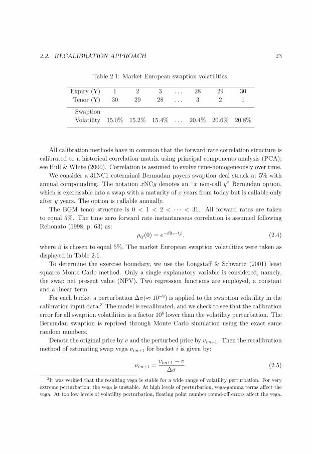
51

2.2. RECALIBRATION APPROACH 23

Table 2.1: Market European swaption volatilities.

Expiry (Y) 1 2 3 . . . 28 29 30

Tenor (Y) 30 29 28 . . . 3 2 1

Swaption

Volatility 15.0% 15.2% 15.4% . . . 20.4% 20.6% 20.8%

All calibration methods have in common that the forward rate correlation structure is

calibrated to a historical correlation matrix using principal components analysis (PCA);

see Hull & White (2000). Correlation is assumed to evolve time-homogeneously over time.

We consider a 31NC1 coterminal Bermudan payers swaption deal struck at 5% with

annual compounding. The notation xNCy denotes an “x non-call y” Bermudan option,

which is exercisable into a swap with a maturity of x years from today but is callable only

after y years. The option is callable annually.

The BGM tenor structure is 0 < 1 < 2 < · · · < 31. All forward rates are taken

to equal 5%. The time zero forward rate instantaneous correlation is assumed following

Rebonato (1998, p. 63) as:

ρij(0) = e−β|ti−tj |, (2.4)

where β is chosen to equal 5%. The market European swaption volatilities were taken as

displayed in Table 2.1.

To determine the exercise boundary, we use the Longstaff & Schwartz (2001) least

squares Monte Carlo method. Only a single explanatory variable is considered, namely,

the swap net present value (NPV). Two regression functions are employed, a constant

and a linear term.

For each bucket a perturbation ∆σ(≈ 10−8) is applied to the swaption volatility in the

calibration input data.3 The model is recalibrated, and we check to see that the calibration

error for all swaption volatilities is a factor 106 lower than the volatility perturbation. The

Bermudan swaption is repriced through Monte Carlo simulation using the exact same

random numbers.

Denote the original price by v and the perturbed price by vi:n+1. Then the recalibration

method of estimating swap vega νi:n+1 for bucket i is given by:

νi:n+1 =vi:n+1 − v

∆σ. (2.5)

3It was verified that the resulting vega is stable for a wide range of volatility perturbation. For veryextreme perturbation, the vega is unstable. At high levels of perturbation, vega-gamma terms affect thevega. At too low levels of volatility perturbation, floating point number round-off errors affect the vega.

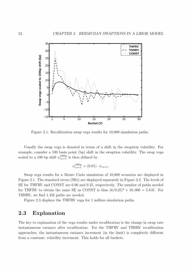
52


1 5 10 15 20 25 30−15

−10

−5

0

5

10

15

20

25

30

35

Bucket (Y)

Sw

ap v

ega

scal

ed t

o 1

00b

p s

hif

t (b

p)

THFRVTHSRVCONST

Figure 2.1: Recalibration swap vega results for 10,000 simulation paths.

Usually the swap vega is denoted in terms of a shift in the swaption volatility. For

example, consider a 100 basis point (bp) shift in the swaption volatility. The swap vega

scaled to a 100 bp shift ν100bpi:n+1 is then defined by

ν100bpi:n+1 = (0.01) · νi:n+1.

Swap vega results for a Monte Carlo simulation of 10,000 scenarios are displayed in

Figure 2.1. The standard errors (SEs) are displayed separately in Figure 2.2. The levels of

SE for THFRV and CONST are 6.00 and 0.25, respectively. The number of paths needed

for THFRV to obtain the same SE as CONST is thus (6/0.25)2 × 10, 000 = 5.8M . For

THSRV, we find 1.4M paths are needed.

Figure 2.3 displays the THFRV vega for 1 million simulation paths.

2.3 Explanation

The key to explanation of the vega results under recalibration is the change in swap rate

instantaneous variance after recalibration. For the THFRV and THSRV recalibration

approaches, the instantaneous variance increment (in the limit) is completely different

from a constant- volatility increment. This holds for all buckets.

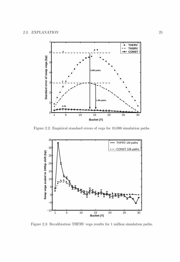
53

2.3. EXPLANATION 25

1 5 10 15 20 25 300

1

2

3

4

5

6

7

Bucket (Y)

Sta

nd

ard

err

or

of

swap

veg

a (b

p)

THFRVTHSRVCONST6

3

0.25

5.8M paths

1.4M paths

Figure 2.2: Empirical standard errors of vega for 10,000 simulation paths.

1 5 10 15 20 25 30−10

−5

0

5

10

15

20

25

30

35

Bucket (Y)

Sw

ap v

ega

scal

ed t

o 1

00b

p s

hif

t (b

p)

THFRV 1M paths CONST 10k paths

Figure 2.3: Recalibration THFRV vega results for 1 million simulation paths.

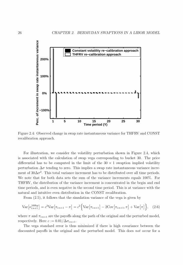
54


1 5 10 15 20 25 30

−100%

0%

100%

200%

Time period (Y)Per

c. o

f inc

rem

ent i

n sw

ap r

ate

inst

anta

neou

s va

rianc

e

Constant volatility re−calibration approachTHFRV re−calibration approach

Figure 2.4: Observed change in swap rate instantaneous variance for THFRV and CONST

recalibration approach.

For illustration, we consider the volatility perturbation shown in Figure 2.4, which

is associated with the calculation of swap vega corresponding to bucket 30. The price

differential has to be computed in the limit of the 30 × 1 swaption implied volatility

perturbation ∆σ tending to zero. This implies a swap rate instantaneous variance incre-

ment of 30∆σ2. This total variance increment has to be distributed over all time periods.

We note that for both data sets the sum of the variance increments equals 100%. For

THFRV, the distribution of the variance increment is concentrated in the begin and end

time periods, and is even negative in the second time period. This is at variance with the

natural and intuitive even distribution in the CONST recalibration.

From (2.5), it follows that the simulation variance of the vega is given by

Var[ν100bp

i:n+1

]= c2Var

[πi:n+1 − π

]= c2

Var

[πi:n+1

]− 2Cov[πi:n+1, π

]+ Var

[π]

, (2.6)

where π and πi:n+1 are the payoffs along the path of the original and the perturbed model,

respectively. Here c := 0.01/∆σi:n+1.

The vega standard error is thus minimized if there is high covariance between the

discounted payoffs in the original and the perturbed model. This does not occur for a

55

2.4. SWAP VEGA AND THE SWAP MARKET MODEL 27

perturbation such as dictated by THFRV, because the stochasticity in the simulation is

basically moved around to other time periods (in our case from period 2 to period 1).

Because the rate increments over different time periods are independent, this leads to a

reduced covariance, leading in turn to a higher standard error of the vega.

There is higher covariance between the payoffs under the perturbations of variance

implied by the CONST calibration, because then each independent time period maintains

approximately the same level of variance; no stochasticity is moved to other random

sources. From (2.6), it then follows that the standard error is lower.

2.4 Swap vega and the swap market model

An alternative method for calculating swap vega has the advantage that the estimates of

vega have a low standard error for any volatility function. The first step is to study the

definition of swap vega in the swap market model, which we will extend to the LIBOR

BGM model. This will give us an alternative method to calculate swap vega per bucket.

How much our dynamically managed hedging portfolio should hold in European swap-

tions is essentially determined by the swap vega per bucket. The latter is the derivative

of the exotic price with respect to the Black swaption implied volatility.

We consider a swap market model S. In the model, swap rates are lognormally dis-

tributed under their forward swap measure. This means that all swap rate volatility

functions σi:n+1(·) of (2.2) are deterministic. The Black implied swaption volatility σk:n+1

is given by

σk:n+1 =

√1

tk

∫ tk

0

|σk:n+1(s)|2ds.

As may be seen in this equation, there are an uncountable number of perturbations of

the swap rate instantaneous volatility that produce the same perturbation as the Black

implied swaption volatility. There is, however, a natural one-dimensional parameterized

perturbation of the swap rate instantaneous volatility, namely, a simple proportional

increment. This is illustrated in Figure 2.5.

We define swap vega in the swap market model as follows. Denote the price of an

interest rate derivative in a swap market model S by v. We consider a perturbation of

the swap rate instantaneous volatility given by

σεk:n+1(·) = (1 + ε)σk:n+1(·), (2.7)

where the shift applies only to k : n+1. Denote the corresponding swap market model by

Sk:n+1(ε). We note that the implied swaption volatility in Sk:n+1(ε) is given by σεk:n+1 =

(1 + ε)σk:n+1. Denote the price of the derivative in Sk:n+1(ε) by vk:n+1(ε). Then the swap

56


0 TTime

Sw

ap r

ate

inst

anta

neo

us

vola

tilit

y

ε

ε

ε σ(⋅)

(1+ε)σ(⋅)

Figure 2.5: Natural increment of Black implied swaption volatility.

vega per bucket νk:n+1 is defined as

νk:n+1 = limε→0

vk:n+1(ε)− v

εσk:n+1

. (2.8)

Equation (2.8) is the derivative of the exotic price with respect to the Black implied

swaption volatility. In conventional notation we may write

νk:n+1 =∂v

∂σk:n+1

= lim∆σk:n+1→0

v(σk:n+1 + ∆σk:n+1)− v(σk:n+1)

∆σk:n+1

(2.9)

In (2.8) εσk:n+1 is equal to the swaption volatility perturbation ∆σk:n+1, and vk:n+1(ε)

and v denote the prices of the derivative in models where the k-th swaption volatility

equals σk:n+1 + ∆σk:n+1 and σk:n+1, respectively.

The swap rate volatility perturbation in (2.7) defines a relative shift. It is also possible

to apply an absolute shift in the form of

σεk:n+1(·) =

(1 +

ε

‖σk:n+1(·)‖)

σk:n+1(·), (2.10)

where the shift applies only to k : n + 1. This ensures that the absolute level of the swap

rate instantaneous volatility is increased by an amount ε. We note that the relative and

57

2.5. ALTERNATIVE METHOD FOR CALCULATING SWAP VEGA 29

absolute perturbation are equivalent when the instantaneous volatility is constant over

time.

The method for calculating swap vega per bucket is largely the same for both relative

and absolute perturbation (but we will point out any differences). The first difference

is in the change in swaption implied volatility ∆σk:n+1 of (2.9); namely, straightforward

calculations reveal that the perturbed volatility satisfies

σεk:n+1 = σk:n+1 + ε

1tk

∫ tk0‖σk:n+1(s)‖ds

σk:n+1

+O(ε2

).

2.5 Alternative method for calculating swap vega

An alternative method for calculating swap vega in the BGM framework may be applied

to any volatility function to yield accurate vega with a small number of simulation paths.

The method is based on a perturbation in the forward rate volatility to match a constant

swap rate volatility increment. Rebonato (2002) also derives this method in terms of

covariance matrices, but our derivation is explicitly in terms of volatility vectors.

Swap rates are not lognormally distributed in the LIBOR BGM model. This means

that swap rate instantaneous volatility is stochastic. The stochasticity is almost invisible

as shown empirically, for example, by Brace et al. (1998). D’Aspremont (2002) shows

that the swap rate is uniformly close to a lognormal martingale.

Hull & White (2000) show that the swap rate volatility vector is a weighted average

of forward LIBOR volatility vectors:

σi:n+1(t) =n∑

j=i

wi:n+1j (t)σj(t), wi:n+1

j (t) =αjγ

i:n+1j (t)fj(t)

1 + αjfj(t), (2.11)

γi:n+1j (t) =

bi(t)

bi(t)− bn+1(t)− pi:j(t)

pi:n+1(t),

where the weights wi:n+1 are in general state-dependent.

Hull and White derive an approximating formula for European swaption prices that

is based on evaluating the weights in (2.11) at time zero. This is a good approximation

by virtue of the near lognormality of swap rates in the LIBOR BGM model. We denote

the resulting swap rate instantaneous volatility by σHWi:n+1 as follows:

σHWi:n+1(t) =

n∑j=i

wi:n+1j (0)σj(t). (2.12)

When we write wi:n+1j := wi:n+1

j (0) and adopt the convention that

σi(t) = σi:n+1(t) = 0 when t > ti,

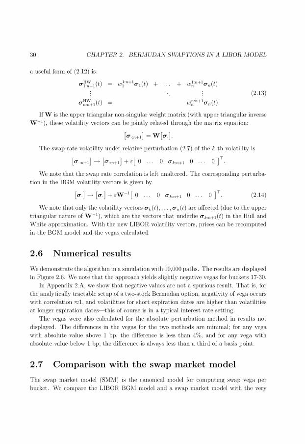
58


a useful form of (2.12) is:

σHW1:n+1(t) = w1:n+1

1 σ1(t) + . . . + w1:n+1n σn(t)

.... . .

...

σHWn:n+1(t) = wn:n+1

n σn(t)

(2.13)

If W is the upper triangular non-singular weight matrix (with upper triangular inverse

W−1), these volatility vectors can be jointly related through the matrix equation:[σ·:n+1

]= W

[σ·

].

The swap rate volatility under relative perturbation (2.7) of the k-th volatility is[σ·:n+1

] → [σ·:n+1

]+ ε

[0 . . . 0 σk:n+1 0 . . . 0

]>.

We note that the swap rate correlation is left unaltered. The corresponding perturba-

tion in the BGM volatility vectors is given by[σ·

] → [σ·

]+ εW−1

[0 . . . 0 σk:n+1 0 . . . 0

]>. (2.14)

We note that only the volatility vectors σk(t), . . . , σn(t) are affected (due to the upper

triangular nature of W−1), which are the vectors that underlie σk:n+1(t) in the Hull and

White approximation. With the new LIBOR volatility vectors, prices can be recomputed

in the BGM model and the vegas calculated.

2.6 Numerical results

We demonstrate the algorithm in a simulation with 10,000 paths. The results are displayed

in Figure 2.6. We note that the approach yields slightly negative vegas for buckets 17-30.

In Appendix 2.A, we show that negative values are not a spurious result. That is, for

the analytically tractable setup of a two-stock Bermudan option, negativity of vega occurs

with correlation ≈1, and volatilities for short expiration dates are higher than volatilities

at longer expiration dates—this of course is in a typical interest rate setting.

The vegas were also calculated for the absolute perturbation method in results not

displayed. The differences in the vegas for the two methods are minimal; for any vega

with absolute value above 1 bp, the difference is less than 4%, and for any vega with

absolute value below 1 bp, the difference is always less than a third of a basis point.

2.7 Comparison with the swap market model

The swap market model (SMM) is the canonical model for computing swap vega per

bucket. We compare the LIBOR BGM model and a swap market model with the very

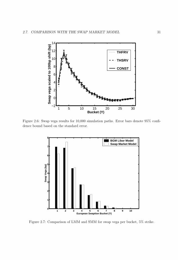
59

2.7. COMPARISON WITH THE SWAP MARKET MODEL 31

1 5 10 15 20 25 30−2

0

2

4

6

8

10

12

14

Bucket (Y)

Sw

ap v

ega

scal

ed t

o 1

00b

p s

hif

t (b

p)

THFRV THSRV CONST

Figure 2.6: Swap vega results for 10,000 simulation paths. Error bars denote 95% confi-

dence bound based on the standard error.

1 2 3 4 5 6 7 8 9 100

1

2

3

4

5

6

7

8

European Swaption Bucket (Y)

Sw

ap V

ega

(bp

)

BGM Libor ModelSwap Market Model

Figure 2.7: Comparison of LMM and SMM for swap vega per bucket, 5% strike.

60


0% 3% 6% 9% 12% 15%

0

5

10

15

20

25

Strike / Fixed Coupon

To

tal S

wap

Veg

a (b

p)

BGM Libor ModelSwap Market Model

Figure 2.8: Comparison of LMM and SMM for total swap vega against strike.

same swap rate quadratic cross-variation structure. Approximate equivalence between

the two models has been established by Joshi & Theis (2002, Equation (3.8)).

We perform the test for an 11NC1 pay-fixed Bermudan option on a swap with annual

fixed and floating payments. A single-factor LIBOR BGM model is used with constant

volatility calibrated to the euro cap volatility curve of October 10, 2001. The zero rates

were taken to be flat at 5%. In the Monte Carlo simulation of the SMM we apply the

discretization suggested in Lemma 5 of Glasserman & Zhao (2000).

Results appear in Table 2.2, and are displayed partially in Figures 2.7 and 2.8. In this

particular case, the BGM LIBOR model reproduces the swap vegas of the swap market

model very accurately.

2.8 Conclusions

We have presented a new approach to calculating swap vega per bucket in the LIBOR

BGM model. We show that for some forms of the volatility an approach based on re-

calibration may lead to great uncertainty in estimated swap vega, as the instantaneous

volatility structure may be distorted by recalibration. This does not happen in the case

of constant swap rate volatility.

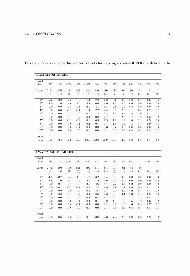
61

2.8. CONCLUSIONS 33

Table 2.2: Swap vega per bucket test results for varying strikes—10,000 simulation paths.

BGM LIBOR MODEL

Fixed

Rate 2% 3% 3.5% 4% 4.5% 5% 6% 7% 8% 9% 10% 12% 15%

Value 2171 1476 1138 829 585 410 210 112 64 36 21 8 2

(4) (5) (5) (5) (5) (4) (3) (2) (2) (1) (1) (1) (0)

1Y -2.0 -2.0 2.6 10.9 11.1 7.0 1.2 0.1 0.0 0.0 0.0 0.0 0.0

2Y 1.5 1.6 1.0 2.6 5.7 6.8 4.0 1.0 0.0 0.0 0.0 0.0 0.0

3Y 0.0 0.0 -0.3 0.1 2.5 4.5 4.1 2.1 1.0 0.3 0.0 0.0 0.0

4Y 0.0 0.0 -0.1 -0.1 1.1 2.7 4.4 3.6 2.0 1.1 0.5 0.2 0.1

5Y 0.0 0.0 -0.1 -0.2 0.4 1.5 3.7 3.6 2.7 1.5 1.0 0.3 0.1

6Y 0.0 0.0 -0.1 -0.2 0.1 0.8 2.1 2.5 2.0 1.7 1.2 0.3 0.2

7Y 0.0 0.0 -0.1 -0.2 0.0 0.3 1.3 1.8 1.8 1.6 1.1 0.5 0.0

8Y 0.0 0.0 0.0 -0.1 -0.1 0.1 0.7 1.3 1.5 1.3 1.3 0.9 0.3

9Y 0.0 0.0 0.0 -0.1 -0.1 0.0 0.3 0.7 0.8 0.8 0.8 0.6 0.3

10Y 0.0 0.0 0.0 0.0 0.0 0.0 0.1 0.3 0.3 0.4 0.4 0.3 0.2

Total

Vega -0.5 -0.4 2.9 12.8 20.8 23.8 21.9 16.9 12.3 8.8 6.2 3.1 1.0

SWAP MARKET MODEL

Fixed

Rate 2% 3% 3.5% 4% 4.5% 5% 6% 7% 8% 9% 10% 12% 15%

Value 2172 1480 1146 841 592 411 204 109 61 34 19 7 1

(6) (6) (6) (5) (5) (4) (4) (3) (2) (1) (1) (1) (0)

1Y -1.9 -0.7 4.4 11.3 11.5 6.2 0.4 0.0 0.0 0.0 0.0 0.0 0.0

2Y 1.6 1.6 1.1 2.2 5.2 7.5 3.6 0.5 0.0 0.0 0.0 0.0 0.0

3Y 0.0 -0.1 -0.4 0.0 2.0 4.6 4.7 2.2 0.6 0.2 0.0 0.0 0.0

4Y 0.0 -0.1 -0.2 -0.1 0.9 2.7 4.8 3.7 1.7 0.8 0.3 0.1 0.0

5Y 0.0 0.0 -0.2 -0.2 0.4 1.6 3.7 3.0 2.3 1.2 0.5 0.1 0.0

6Y 0.0 0.0 -0.1 -0.2 0.1 0.8 2.6 3.3 3.1 2.3 1.2 0.2 0.0

7Y 0.0 0.0 -0.1 -0.2 -0.1 0.3 1.3 2.0 1.9 1.3 1.4 0.8 0.1

8Y 0.0 0.0 0.0 -0.1 -0.1 0.1 0.8 1.3 1.5 1.5 1.2 0.6 0.2

9Y 0.0 0.0 0.0 -0.1 -0.1 0.0 0.4 0.9 1.0 1.0 0.9 0.7 0.3

10Y 0.0 0.0 0.0 0.0 0.0 0.0 0.1 0.3 0.4 0.5 0.5 0.4 0.3

Total

Vega -0.3 0.6 4.5 12.6 19.9 23.8 22.3 17.2 12.5 8.8 6.0 2.9 0.9

62


We derive an alternative approach that is not based on recalibration, using the swap

market model. The method accurately estimates swaption vegas for any volatility function

and at a small number of simulation paths.

The key to the method is that the perturbation in the LIBOR volatility is distributed

in a clear, stable, and well-understood fashion, but in the recalibration method the change

in volatility is hidden and potentially unstable. We also show for a Bermudan swaption

deal that our method yields almost the same swap vega as a swap market model.

2.A Appendix: Negative vega for two-stock Bermu-

dan options

We examine a two-stock Bermudan option to show that its vega per bucket is negative in

certain situations. The holder of a two-stock Bermudan option has the right to call the

first stock s1 at strike k1 at time t1; if the holder decides to hold the option, the right

remains to call the second stock s2 at strike k2 at time t2; if this right is not exercised,

then the option becomes worthless. Here t1 < t2.

The Bermudan option is valued under standard Black-Scholes conditions. Under the

risk-neutral measure, the stock prices satisfy the stochastic differential equations:

dsi

si

= rdt + σidwi, i = 1, 2, dw1dw2 = ρdt,

where σi is the volatility of the i-th stock, and wi, i = 1, 2, are Brownian motions under

the risk-neutral measure, with correlation ρ. It follows that the time t1 stock prices are

distributed as follows:

si(t1) = f(si(0), 0; t1

)exp

σi

√t1zi − 1

2σ2

i t1

, i = 1, 2, (2.15)

where the pair (z1, z2) is standard bivariate normally distributed with correlation ρ and

where

f(s, t; u) := s expr(u− t)

, (2.16)

is the time t forward price for delivery at time u of a stock with current price s.

At time t1, the holder of the Bermudan option will choose whichever of two alternatives

has a higher value: either calling the first stock, or holding the option on the second stock;

the value of the latter is given by the Black-Scholes formula. on conditioning and involves

a one-dimensional numerical integration over the Black formula.

Therefore the (cash-settled) payoff v(s1(t1), s2(t1), t1) of the Bermudan at time t1 is

given by:

max(

s1(t1)− k1

)+, BS2

(s2(t1), t1

), (2.17)

63

2.A. APPENDIX: NEGATIVE VEGA TWO-STOCK BERMUDAN OPTIONS 35

Table 2.3: Deal description.

Spot price for stock 1 s1(0) 150

Spot price for stock 2 s2(0) 140

Strike price for stock 1 k1 100

Strike price for stock 2 k2 100

Exercise time for stock 1 t1 1Y

Exercise time for stock 2 t2 2Y

Volatilities σi Variable

Correlation ρ 0.9

Risk-free rate r 5%

where BS is the Black-Scholes formula:

BSi(s, t) = e−r(ti−t)

f(s, t; ti)φ

(d

(i)1

)− kiφ

(d

(i)2

),

d(i)1,2(s, t) =

ln(f(s, t; ti)/ki

)± 12σ2

i t

σi

√t

,

where φ(·) is the cumulative normal distribution function.

The time zero value v(s1, s2, 0) of the Bermudan option may thus be computed by a

bivariate normal integration of the discounted version of the payoff in (2.17):

v(s1, s2, 0) = e−rt1E[v(t1, s1(t1), s2(t1)

)].

The vega per bucket νi is defined as

νi :=∂v(s1, s2, 0)

∂σi

, i = 1, 2.

The vega may be numerically approximated by finite differences:

νi =v(s1, s2, 0; σi + ∆σi)− v(s1, s2, 0; σi)

∆σi

+O(∆σ2

i

), i = 1, 2,

for a small volatility perturbation ∆σi ¿ 1.

We note that the vega per bucket may possibly be negative for both the first and the

second bucket. As an example of vega negativity, we compute the vega per bucket for the

deal described in Table 2.3. Results are displayed in Table 2.4. The volatility is perturbed

by a small amount.

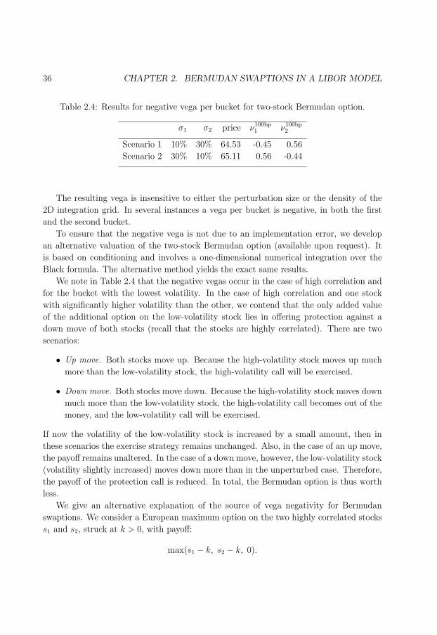
64


Table 2.4: Results for negative vega per bucket for two-stock Bermudan option.

σ1 σ2 price ν100bp1 ν100bp

2

Scenario 1 10% 30% 64.53 -0.45 0.56

Scenario 2 30% 10% 65.11 0.56 -0.44

The resulting vega is insensitive to either the perturbation size or the density of the

2D integration grid. In several instances a vega per bucket is negative, in both the first

and the second bucket.

To ensure that the negative vega is not due to an implementation error, we develop

an alternative valuation of the two-stock Bermudan option (available upon request). It

is based on conditioning and involves a one-dimensional numerical integration over the

Black formula. The alternative method yields the exact same results.

We note in Table 2.4 that the negative vegas occur in the case of high correlation and

for the bucket with the lowest volatility. In the case of high correlation and one stock

with significantly higher volatility than the other, we contend that the only added value

of the additional option on the low-volatility stock lies in offering protection against a

down move of both stocks (recall that the stocks are highly correlated). There are two

scenarios:

• Up move. Both stocks move up. Because the high-volatility stock moves up much

more than the low-volatility stock, the high-volatility call will be exercised.

• Down move. Both stocks move down. Because the high-volatility stock moves down

much more than the low-volatility stock, the high-volatility call becomes out of the

money, and the low-volatility call will be exercised.

If now the volatility of the low-volatility stock is increased by a small amount, then in

these scenarios the exercise strategy remains unchanged. Also, in the case of an up move,

the payoff remains unaltered. In the case of a down move, however, the low-volatility stock

(volatility slightly increased) moves down more than in the unperturbed case. Therefore,

the payoff of the protection call is reduced. In total, the Bermudan option is thus worth

less.

We give an alternative explanation of the source of vega negativity for Bermudan

swaptions. We consider a European maximum option on the two highly correlated stocks

s1 and s2, struck at k > 0, with payoff:

max(s1 − k, s2 − k, 0).

65

2.A. APPENDIX: NEGATIVE VEGA TWO-STOCK BERMUDAN OPTIONS 37

We deem the risk behaviour of this option to be similar to the risk behaviour of a Bermu-

dan swaption, since the choice of calling either s1 or s2 corresponds to the choice of

exercising at the first or second exercise opportunity. We have:

max(s1 − k, s2 − k, 0) = max(s1 − k, 0) + 1s1>k max(s2 − s1, 0).

The maximum option is thus the sum of an ordinary European call option and a (con-

ditional) European spread option. If the volatility of the first stock increases then the

volatility of the spread s2− s1 decreases (for highly correlated stocks), by which the value

of the European spread option decreases. This causes a negative component in the to-

tal composition of the vega. However the ordinary call option value increases when the

volatility of the first stock increases, which thus constitutes a positive component of the

vega.

The same argument can be applied to show that an increase in volatility of the second

stock causes a negative component in the vega. The spread option argument carefully

shows a negative component in the vega of a Bermudan swaption, however it does not

explain that this negative component can sometimes outweigh the other positive compo-

nents of the vega. This outweighing of the negative component is explained in the up and

down moves argument above.

66

67

Chapter 3

Rank reduction of correlation

matrices by majorization

1 A novel algorithm is developed for the problem of finding a low-rank correlation ma-

trix nearest to a given correlation matrix. The algorithm is based on majorization and,

therefore, it is globally convergent. The algorithm is computationally efficient, is straight-

forward to implement, and can handle arbitrary weights on the entries of the correlation

matrix. A simulation study suggests that majorization compares favourably with compet-

ing approaches in terms of the quality of the solution within a fixed computational time.

The problem of rank reduction of correlation matrices occurs when pricing a derivative

dependent on a large number of assets, where the asset prices are modelled as correlated

log-normal processes. Such an application mainly concerns interest rates.

3.1 Introduction

In this chapter, we study the problem of finding a low-rank correlation matrix nearest

to a given (correlation) matrix. First we explain how this problem occurs in an interest

rate derivatives pricing setting. We will focus on interest rate derivatives that depend on

several rates such as the 1 year LIBOR deposit rate, the 2 year swap rate, etc. An example

of such a derivative is a Bermudan swaption. A Bermudan swaption gives its holder the

right to enter into a fixed maturity interest rate swap at certain exercise dates. At an

exercise opportunity, the holder has to choose between exercising then or holding onto the

option with the chance of entering into the swap later at more favourable interest rates.

1This chapter has been published in different form as Pietersz, R. & Groenen, P. J. F. (2004b), ‘Rankreduction of correlation matrices by majorization’, Quantitative Finance 4(6), 649–662. An extendedabstract of this chapter appeared as Pietersz, R. & Groenen, P. J. F. (2004a), ‘A major LIBOR fit’, RiskMagazine p. 102. December issue.

68

40 CHAPTER 3. RANK REDUCTION BY MAJORIZATION

Evidently, the value depends not only on the current available swap rate but, amongst

others, also on the forward swap rates corresponding to future exercise dates. In contrast,

an example of a derivative that is dependent on a single interest rate is a caplet, which

can be viewed as a call option on LIBOR. In this case, the value of the caplet depends

only on a single forward LIBOR rate.

Here, we will focus on derivatives depending on several rates. Our discussion can

however also be applied to the situation of a derivative depending on several assets. To

do so a model is set up that specifies the behaviour of the asset prices. Each of the

asset prices is modelled as a log-normal martingale under its respective forward measure.

Additionally, the asset prices are correlated. Suppose we model n correlated log-normal

price processes,dsi

si

= . . . dt + σidwi, 〈dwi, dwj〉 = ρij, (3.1)

under a single measure. Here si denotes the price of the ith asset, σi its volatility and wi

denotes the associated driving Brownian motion. Brownian motions i and j are correlated

with coefficient ρij, the correlation coefficient between the returns on assets i and j. The

matrix P = (ρij)ij should be positive semidefinite and should have a unit diagonal. In

other words, P should be a true correlation matrix. The term . . . dt denotes the drift

term that stems from the change of measure under the non-arbitrage condition.

The models that fit into the framework of (3.1) and which are most relevant to our

discussion are the LIBOR and swap market models for valuation of interest rate deriva-

tives, as introduced in Section 1.3.2. These models were developed by Brace et al. (1997),

Jamshidian (1997) and Miltersen et al. (1997). In this case, an asset price corresponds to

a forward LIBOR or swap rate. For example, if we model a 30 year Bermudan swaption

with annual call and payment dates, then our model would consist of 30 annual forward

LIBOR rates or 30 co-terminal forward swap rates. In the latter case, we consider 30 for-

ward starting annual-paying swaps, starting at each of the 30 exercise opportunities and

all ending after 30 years. Model (3.1) could however be applied to a derivative depending

on a number of, for example, stocks, too.

Given the model (3.1), the price of any derivative depending on the assets can be

calculated by non-arbitrage arguments. Because the number of assets is assumed to be

high and the derivative is assumed complex in this exposition, the derivative value can be

calculated only by Monte Carlo simulation. To implement scheme (3.1) by Monte Carlo

we need a decomposition P = YYT , with Y an n × n matrix. In other words, if we

denote the ith row vector of Y by yi, then the decomposition reads 〈yi,yj〉 = ρij, where

〈., .〉 denotes the scalar product. We then implement the scheme

dsi

si

= . . . dt + σi

yi1dw1 + · · ·+ yindwn

, 〈yi,yj〉 = ρij, (3.2)

69

3.1. INTRODUCTION 41

where the wi are now independent Brownian motions. Scheme (3.2) indeed corresponds

to scheme (3.1) since both volatility and correlation are implemented correctly. The

instantaneous variance is 〈dsi/si〉 = σ2i dt since ‖yi‖ = ρii = 1 and volatility is the square

root of instantaneous variance divided by dt. Moreover, for the instantaneous covariance

we have 〈dsi/si, dsj/sj〉 = σiσj〈yi,yj〉dt = σiσjρijdt.

For large interest rate correlation matrices, usually almost all variance (say 99%) can

be attributed to only 3–6 stochastic Brownian factors. Therefore, (3.2) contains a large

number of almost redundant Brownian motions that cost expensive computational time

to simulate. Instead of taking into account all Brownian motions, we would wish to do

the simulation with a smaller number of factors, d say, with d < n and d typically between

2 and 6. The scheme then becomes

dsi

si

= . . . dt + σi

yi1dw1 + · · ·+ yiddwd

, 〈yi,yj〉 = ρij. (3.3)

The n×d matrix Y is a decomposition of P. This approach immediately implies that the

rank of P be less than or equal to d. For financial correlation matrices, this rank restric-

tion is generally not satisfied. It follows that an approximation be required. We could

proceed in two possible ways. The first way involves approximating the covariance matrix

(σiσjρij)ij. The second involves approximating the correlation matrix while maintaining

an exact fit to the volatilities. In a derivatives pricing setting, usually the volatilities

are well-known. These can be calculated via a Black-type formula from the European

option prices quoted in the market, or mostly these volatilities are directly quoted in the

market. The correlation is usually less known and can be obtained in two ways. First, it

can be estimated from historical time series. Second, it can be implied from correlation

sensitive market-traded options such as spread options. A spread option is an option on

the difference between two rates or asset prices. Such correlation sensitive products are

not traded as liquidly as the European plain-vanilla options. Consequently, in both cases

of historic or market-implied correlation, we are more confident of the volatilities. For

that reason, in a derivative pricing setting, we approximate the correlation matrix rather

than the covariance matrix.

The above considerations lead to solving the following problem:

Find Y ∈ Rn×d,

to minimize ϕ(Y) := 1c

∑i<j wij

(ρij − 〈yi,yj〉

)2,

subject to ‖yi‖2 = 1, i = 1, . . . , n.

(3.4)

Here wij are nonnegative weights and c := 4∑

i<j wij. The objective value ϕ is scaled

by the constant c in order to make it independent of the problem dimension n. Because

each term ρij − 〈yi,yj〉 is always between 0 and 2, it follows for the choice of c that ϕ is

always between 0 and 1.

70


An interesting alternative is to approximate the covariance matrix while keeping vari-

ance fixed2. If P = (ρij)ij denotes the instantaneous covariance matrix, and σ denotes

the vector of volatilities, then

P = Diag(σ) P Diag(σ),

where Diag(σ) denotes a diagonal matrix with the diagonal filled with the vector σ.

Approximating the covariance matrix while ensuring a perfect fit to variance amounts to

solving the following problem (we leave out weights w and the scalar factor c, from (3.4),

for clarity of presentation):

Find Y ∈ Rn×d,

to minimize ϕ(Y) :=∑

i<j

(ρij − 〈yi, yj〉

)2,

subject to ‖yi‖22 = ρii, i = 1, . . . , n.

(3.5)

Here, yi relates to yi in (3.3) via

yi = σiyi.

Approximating covariance with fixed variance as in (3.5) yields, in general, different results

than approximating correlation as in (3.4), since the added variance may change the

importance of certain factors. We carefully state “in general” and “may change”, since

if all variances are equal to one, then problems (3.4) (with constant weights) and (3.5)

are obviously identical. We note that the majorization algorithm in this chapter, and

the geometric programming algorithm in Chapter 4, can be applied to the covariance

approximating problem in (3.5) by setting the weights in (3.4) as wij = σ2i σ

2j . The

covariance problem (3.5) is thus a special case of the correlation problem (3.4), therefore

we focus on (3.4) in the remainder of the thesis.

The weights wij in (3.4) have been added for three reasons:

• For squared differences, a large difference constitutes a far greater part of the total

error in (3.4) than a small difference. The weights for small differences can then be

appropriately increased to adjust for this.

• Financial reasons may sometimes compel us to assign higher weights to particular

correlation pairs. For example, we could be more confident about the correlation

between the 1 and 2 year swap rates than about the correlation between the 8 and

27 year swap rates.

• The objective function with weights has been considered before in the literature.

See for example Rebonato (1999c, Section 10). Rebonato (2002, Section 9) provides

an excellent discussion of the pros and cons of using weights.

2Many thanks to Ton Vorst for pointing out this alternative.

71

3.2. LITERATURE REVIEW 43

The simplest case of ϕ is ϕ(Y) := c−1‖P −YYT‖2F , where ‖ · ‖F denotes the Frobenius

norm, ‖Y‖2F := tr(YYT ) for matrices Y. This objective function (which we shall also call

‘Frobenius norm’) fits in the framework of (3.4); it corresponds to the case of all weights

equal. The objective function in (3.4) will be referred to as ‘general weights’.

In the literature, there exist six other algorithms for minimizing ϕ defined in (3.4).

These methods are outlined in the next section and are shown to have several disadvan-

tages, namely none of the methods is simultaneously

(i) efficient,

(ii) straightforward to implement,

(iii) able to handle general weights and

(iv) guaranteed to converge to a local minimum.

In this chapter, we develop a novel method to minimize ϕ that simultaneously has the

four mentioned properties. The method is based on iterative majorization that has the

important property of guaranteed convergence to a stationary point. The algorithm is

straightforward to implement. We show that the method can efficiently handle general

weights. We investigate empirically the efficiency of majorization in comparison to other

methods in the literature. The benchmark tests that we will consider are based on the

performance given a fixed small amount of computational time. This is exactly the situ-

ation in practice: decisions based on derivative pricing calculations have to be made in a

limited amount of time.

The remainder of this chapter is organized as follows. First, we provide an overview

of the methods available in the literature. Second, the idea of majorization is introduced

and the majorizing functions are derived. Third, an algorithm based on majorization is

given along with reference to associated MATLAB code. Global convergence and the local

rate of convergence are investigated. Fourth, we present empirical results. The chapter

ends with some conclusions.

3.2 Literature review

We describe seven existing algorithms available in the literature for minimizing ϕ. Because

a review of the majorization method is interesting from the point of view of Chapter

4 (Rank reduction by geometric programming), we include here the discussion of the

majorization method itself. For each of the seven algorithms, it is indicated whether

it can handle general weights. If not, then the most general objective function it can

handle stems from the weighted Frobenius norm ‖ · ‖F,Ω with Ω a symmetric positive

72


definite matrix, where ‖Y‖2F,Ω := tr(YΩYTΩ). The objective function ϕ(Y) := c−1‖R−

YYT‖2F,Ω will be referred to as ‘weighted Frobenius norm’ too.

3.2.1 Modified PCA

First, we mention the ‘modified principal component analysis (PCA)’ method. For ease

of exposition, we restrict to the case of the Frobenius norm, however the method can be

applied to the weighted Frobenius norm as well though not for general weights. Modified

PCA is based on an eigenvalue decomposition P = QΛQT , with Q orthogonal and Λ

the diagonal matrix with eigenvalues. If the eigenvalues are ordered descendingly then a

low-rank decomposition with associated approximated matrix close to the original matrix

is found by

YPCAi =z

‖z‖2

, (3.6)

z :=QdΛ

1/2d

i, i = 1, . . . , n. (3.7)

Here Xi denotes the ith row of a matrix X, Qd the first d columns of Q, and Λd the

principal sub-matrix of Λ of degree d. Ordinary PCA stops with (3.7) and it is the scaling

in (3.6) that is the ‘modified’ part, ensuring that the resulting correlation matrices have

unit diagonal. Modified PCA is popular among financial practitioners and implemented

in numerous financial institutions. The modification of PCA in this way is believed to

be due to Flury (1988). For a description in finance related articles, see, for example,

Sidenius (2000) and Hull & White (2000). Modified PCA is easy to implement, because

almost all that is required is an eigenvalue decomposition. The calculation is almost

instant, and the approximation is reasonably accurate. A strong drawback of modified

PCA is its non-optimality: generally one may find decompositions Y (even locally) for

which the associated correlation matrix YYT is closer to the original matrix P than the

PCA-approximated correlation matrix YPCAYTPCA. The modified PCA approximation

becomes worse when the magnitude of the left out eigenvalues increases.

Throughout this chapter we choose the starting point of any method considered (be-

yond modified PCA) to be the modified PCA solution.

3.2.2 Majorization

Second, we mention the majorization approach of Pietersz & Groenen (2004a, b), see

also this Chapter 3. Majorization can handle an entry-weighted objective function and is

guaranteed to converge to a stationary point. The rate of convergence is sub-linear.

73

3.2. LITERATURE REVIEW 45

3.2.3 Geometric programming

The third algorithm that we discuss, is the geometric programming approach of Grubisic

& Pietersz (2005), see also Chapter 4. Here, the constraint set is equipped with a differ-

entiable structure. Subsequently geometric programming is applied, which can be seen

as Newton-Rhapson or conjugate gradient over curved space. By formulating these algo-

rithms entirely in terms of differential geometric means, a simple expression is obtained

for the gradient. The latter allows for an efficient implementation. Another advantage

of geometric programming is that it can handle general weights. However, a drawback of

the geometric programming approach is that it takes many lines of non-straightforward

code to implement, which may hinder its use for non-experts.

3.2.4 Alternating projections without normal correction

Fourth, we consider the alternating projections algorithm of Grubisic (2002) and Morini

& Webber (2004). The discussion below of alternating projections applies only to the

problem of rank reduction of correlation matrices. The method is based on alternating

projections onto the set of n × n matrices with unit diagonal and onto the set of n × n

matrices of rank d or less. Both these projections can be efficiently calculated. For

projection onto the intersection of two convex sets, Dykstra (1983) and Han (1988) have

shown that convergence to a minimum can be obtained with alternating projections onto

the individual convex sets if a normal vector correction is applied. Their results do not

automatically hold for an alternating projections algorithm with normal correction for

Problem (4.1)3, since for d < n the set of n× n matrices of rank d or less is non-convex.

The alternating projections algorithm could in principle be extended to the case with rank

restrictions, since we can efficiently calculate the projection onto the set of rank-d matrices.

Convergence of the algorithm is however no longer guaranteed by the general results of

Dykstra (1983) and Han (1988) because the constraint set rank(C) ≤ d is no longer

convex for d < n. Some preliminary experimentation showed indeed that the extension

to the non-convex case did not work generally. Also, Morini & Webber (2004) report

that alternating projections with normal correction may fail in solving Problem (4.1).

Higham (2002, Section 5, ‘Concluding remarks’) mentions that he has been investigating

alternative algorithms, such as to include rank constraints. The alternating projections

algorithm without normal correction stated in Grubisic (2002) and Morini & Webber

(2004) however always converges to a feasible point, but not necessarily to a stationary

point. In fact, in general, the alternating projections method without normal correction

does not converge to a stationary point. The algorithm thus does not minimize the

3The algorithm with normal correction for rank reduction has also been studied in Weigel (2004).

74


objective function in (4.1), it only selects a feasible point satisfying the constraints of

(4.1).

3.2.5 Lagrange multipliers

As the fifth algorithm, we mention the Lagrange multiplier technique developed by Zhang

& Wu (2003) and Wu (2003). This method lacks guaranteed convergence: Zhang & Wu

(2003, Proposition 4.1) and Wu (2003, Theorem 3.4) prove the following result. The

Lagrange multiplier algorithm produces a sequence of multipliers for which accumulation

points exist. If, for the original matrix plus the Lagrange multipliers of an accumulation

point, the dth and (d + 1)th eigenvalues have different absolute values, then the resulting

rank-d approximation is a global minimizer of problem (3.4). However, the condition

that the dth and (d + 1)th eigenvalues are different has not been guaranteed. In numeri-

cal experiments, this equal-eigenvalues phenomenon occurs. Therefore, convergence of the

Lagrange multiplier method to a global minimum or even to a stationary point is not guar-

anteed. It is beyond the scope of this chapter to indicate how often this ‘non-convergence’

occurs. If the algorithm has not yet converged, then the produced low-rank correlation

matrix will not satisfy the diagonal constraint. The appropriate adaptation is to re-scale

the associated configuration similarly to the modified PCA approach (3.6). For certain

numerical settings, the resulting algorithm has been shown to perform not better and even

worse than the geometric programming approach (Grubisic & Pietersz 2005). Another

drawback of the Lagrange multiplier algorithm is that only the weighted Frobenius norm

can be handled and not general weights.

3.2.6 Parametrization

Sixth, we mention the ‘parametrization method’ of Rebonato (1999a, 1999b, 1999c (Sec-

tion 10), 2002 (Section 9), 2004b (Sections 20.1–20.4)), Brigo (2002), Brigo & Mercurio

(2001, Section 6.9) and Rapisarda, Brigo & Mercurio (2002). The set of correlation

matrices of rank d or less YYT : Y ∈ Rn×d,Diag(YYT )= I is parameterized by

trigonometric functions through spherical coordinates yi = yi(θi) with θi ∈ Rd−1. As

a result, the objective value ϕ(Y) becomes a function ϕ(Y(Θ)) of the angle parameters

Θ that live in Rn×(d−1). Subsequently, ordinary non-linear optimisation algorithms may

be applied to minimize the objective value ϕ(Y(Θ)) over the angle parameters Θ. In

essence, this approach is the same as geometric optimisation, except for the key difference

of optimising over Θ versus over Y. The major benefit of geometric optimisation over the

parametrization method is as follows. We consider, for ease of exposition, the case of equal

weights. The differential ϕY, in terms of Y, is given simply as 2ΨY, with Ψ = YYT −P,

see (4.24) below. We note that ϕY = 2ΨY can thus be efficiently calculated. The dif-

75

3.3. MAJORIZATION 47

ferential ϕΘ, in terms of Θ however, is 2ΨY multiplied by the differential of Y with

respect to Θ, by the chain rule of differentiation. The latter differential is less efficient to

calculate since it involves numerous sums of trigonometric functions. Grubisic & Pietersz

(2005, Section 6) have shown empirically for a particular numerical setting with many

randomly generated correlation matrices that the parametrization method is numerically

less efficient than either the geometric programming approach or the Lagrange multiplier

approach. The parametrization approach can handle general weights.

3.2.7 Alternating projections with normal correction (d = n)

The seventh important contribution is due to Higham (2002). The algorithm of Higham

(2002) is the alternating projection algorithm with normal correction applied to the case

d = n, i.e., to the problem of finding the nearest (possibly full-rank) correlation matrix.

This method can only be used when there are no rank restrictions (d := n) and only with

the weighted Frobenius norm. To understand the methodology, note that minimization

Problem (3.4) with equal weights and d := n can be written as min‖P − C‖2F ; C º

0, Diag(C) = I. The two constraint sets C º 0 and Diag(C) = I are both convex.

The convexity was cleverly exploited by Higham (2002), in which it was shown that the

alternating projections algorithm of Dykstra (1983) and Han (1988) could be applied. The

same technique has been applied in a different context in Chu, Funderlic & Plemmons

(2003), Glunt, Hayden, Hong & Wells (1990), Hayden & Wells (1988) and Suffridge &

Hayden (1993). Since the case d < n is the primary interest of this chapter, the method

of Higham (2002) will not be considered in the remainder.

3.3 Majorization

In this section, we briefly describe the idea of majorization and apply majorization to

the objective function ϕ of Problem (3.4). The idea of majorization has been described,

amongst others, in De Leeuw & Heiser (1977), Kiers & Groenen (1996) and Kiers (2002).

We follow here the lines of Borg & Groenen (1997, Section 8.4). The key to majorization

is to find a simpler function that has the same function value at a supporting point x

and anywhere else is larger than or equal to the objective function to be minimized. Such

a function is called a majorization function. By minimizing the majorization function –

which is an easier task since this function is ‘simpler’ – we obtain the next point of the

algorithm. This procedure guarantees that the function value never increases along points

generated by the algorithm. Moreover, if the objective and majorization functions are once

continuously differentiable (which turns out to hold in our case), then the properties above

imply that the gradients should match at the supporting point x. As a consequence,

from any point where the gradient of the objective function is non-negligible, iterative

76


majorization will be able to find a next point with a strictly smaller objective function

value. This generic fact for majorization algorithms has been pointed out in Heiser (1995).

We formalize the procedure somewhat more. Let ϕ(·) denote the function to be min-

imized. Let for each x in the domain of ϕ be given a majorization function χ(·,x) such

that

(i) ϕ(x) = χ(x,x),

(ii) ϕ(y) ≤ χ(y,x) for all y, and

(iii) the function χ(·,x) is ‘simple’, that is, it is straightforward to calculate the minimum

of χ(·,x).

A majorization algorithm is then given by

(i) Start at y(0). Set k := 0.

(ii) Set y(k+1) equal to the minimum argument of the function χ(·,y(k)

).

(iii) If ϕ(y(k)

)− ϕ(y(k+1)

)< ε then stop with y := y(k+1).

(iv) Set k := k + 1 and repeat from (ii).

Figure 3.1 illustrates the majorization algorithm.

Below we derive the majorizing function for ϕ(·) in (3.4). The first step is to majorize

ϕ(X) as a function of the ith row only and then to repeat this for each row. To formalize

the notion of ‘ϕ(X) as a function of the ith row only’ we introduce the notation ϕi(y;Y)

to denote the function

ϕi(·,Y) : y 7→ ϕ(Yi(y)

),

for (column)vectors y ∈ Rd with Yi(y) denoting the matrix Y with the ith row replaced

by yT . We interpret Y as [y1 · · ·yn]T . We find

ϕ(Y) =1

c

∑j1<j2

wj1j2

(ρj1j2 − 〈yj1 ,yj2〉

)2

=1

c

∑j1<j2

wj1j2

(ρ2

j1j2+ (yT

j1yj2)

2 − 2ρj1j2yTj1yj2

)

= (const in yi) +1

c

yT

i

[∑

j:j 6=i

wijyjyTj

]yi

︸︷︷︸(I)

− 2yTi

[∑

j:j 6=i

wijρijyj

]

︸︷︷︸(II)

. (3.8)

77

3.3. MAJORIZATION 49

y0y1y2

(.)

(.,y0)

(.,y1)

(y0)= (y0,y0)

(y1,y0)

(y1)= (y1,y1)

(y2,y1)

(y2)

Figure 3.1: The idea of majorization. (Figure adopted from Borg & Groenen (1997,

Figure 8.4).) The algorithm sets out at y0. The majorization function χ(·,y0) is fitted by

matching the value and first derivative of ϕ(·) at y0. Subsequently the function χ(·,y0) is

minimized to find the next point y1. This procedure is repeated to find the point y2 etc.

78


Part (I) is quadratic in yi whereas part (II) is linear in yi; the remaining term is constant

in yi. We only have to majorize part (I), as follows. Define

Bi(Y) :=∑

j:j 6=i

wij yj yTj . (3.9)

For notational convenience, we shall denote Bi(Y) by B, the running yi by y, and the

current yi, that is, the current ith row vector of Y, is denoted by x. Let λ denote the

largest eigenvalue of B. Then, the matrix B − λI is negative semidefinite, so that the

following inequality holds:

(y − x)T (B− λI)(y − x) ≤ 0, ∀y,

which gives after some manipulations

yTBy ≤ 2λ− 2yT (λx−Bx)− xTBx, ∀y, (3.10)

using the fact that yTy = xTx = 1.

Combining (3.8) and (3.10) we obtain the majorizing function of ϕi(y;Y), that is,

ϕi(y;Y) ≤ −2

cyT

(λx−Bx +

∑

j:i6=j

wijρijyj

)+ (const in y) = χi(y;Y), ∀y.

The advantage of χi(·;Y) over ϕi(·,Y) is that it is linear in y and that the minimization

problem

min

χi(y;Y) ; ‖y‖2 = 1

(3.11)

is readily solved by

y∗ := z/‖z‖2, z := λx−Bx +∑

j:j 6=i

wijρijyj.

If z = 0 then this implies that the gradient is zero, from which it would follow that the

current point x is already a stationary point.

3.4 The algorithm and convergence analysis

Majorization algorithms are known to converge to a point with negligible gradient. This

property holds also for the current situation, as will be shown hereafter. As the conver-

gence criterion is defined in terms of the gradient Gradϕ, an expression for Gradϕ is

needed. We restrict to the case of all wij equal. As shown in Grubisic & Pietersz (2005)

(see also Section 4.5.3), the gradient is then given by

Gradϕ = 4c−1ΨY, Ψ := YYT −P. (3.12)

79

3.4. THE ALGORITHM AND CONVERGENCE ANALYSIS 51

Algorithm 1 The majorization algorithm for finding a low-rank correlation matrix locally

nearest to a given matrix. Here P denotes the input matrix, W denotes the weight matrix,

n denotes its dimension, d denotes the desired rank, ε‖Gradϕ‖ is the convergence criterion

for the norm of the gradient and εϕ is the convergence criterion on the improvement in

the function value.Input: P, W, n, d, ε‖Gradϕ‖, εϕ.

1: Find starting point Y by means of the modified PCA method (3.6)–(3.7).

2: for k = 0, 1, 2, ... do

3: stop if the norm of the gradient of ϕ at X(k) := X is less than ε‖Gradϕ‖ and the

improvement in the function value ϕk−1/ϕk − 1 is less than εϕ.

4: for i = 1, 2, ..., n do

5: Set B :=∑

j 6=i wijyjyTj .

6: Calculate λ to be the largest eigenvalue of the d× d matrix B.

7: Set z := λyi −Byi +∑

j 6=i wijρijyj.

8: If z 6= 0, then set the ith row yi of Y equal to z/‖z‖2.

9: end for

10: end for

Output: the n×n matrix YYT is the rank-d approximation of P satisfying the convergence

constraints.

An expression for the gradient for the objective function with general weights can be

found by straightforward differentiation. The majorization algorithm has been displayed

in Algorithm 1.

The row-wise approach of Algorithm 1 makes it dependent of the order of looping

through the rows. This order effect will be addressed in Section 3.5.3. In Sections 3.5.4

and 3.5.5 we study different ways of implementing the calculation of the largest eigenvalue

of B in line 6 of Algorithm 1. In particular, we study the use of the power method.

In the remainder of this section the convergence of Algorithm 1 is studied. First, we

establish global convergence of the algorithm. Second, we investigate the local rate of

convergence.

3.4.1 Global convergence

Zangwill (1969) developed generic sufficient conditions that guarantee convergence of

an iterative algorithm. The result is repeated here in a form adapted to the case of

majorization. Let M be a compact set. Assume the specification of a subset S ⊂ M

called the solution set. A point Y ∈ S is deemed a solution. An (autonomous) iterative

algorithm is a map A : M → M ∪ stop such that A−1(stop) = S. The proof of the

following theorem is adapted from the proof of Theorem 1 in Zangwill (1969).

80


Theorem 1 (Global convergence) Consider finding a local minimum of the objective

function ϕ(Y) by use of Algorithm 1. Suppose given a fixed tolerance level ε on the

gradient of ϕ. A point Y is called a solution if ‖Gradϕ(Y)‖ < ε. Then from any start-

ing point Y(0), the algorithm either stops at a solution or produces an infinite sequence of

points none of which are solutions, for which the limit of any convergent subsequence is a

solution point.

PROOF: Without loss of generality we may assume that the procedure generates an

infinite sequence of points Y(k) none of which are solutions. It remains to be proven

that the limit of any convergent subsequence must be a solution.

First, note that the algorithm A(·) is continuous in Y. Second, note that if Y(k) is

not a solution then

ϕ(Y(k+1)

)= ϕ

(A

(Y(k)

))< ϕ

(Y(k)

).

Namely if Y(k) is not a solution then its gradient is non-negligible. Since the objective and

all majorization functions are differentiable, we necessarily have that the gradients agree

at Y(k). Therefore, when minimizing the majorization functions χi(·,Y) there will be at

least one i for which we find a strictly smaller objective value. Thus Y(k+1) := A(Y(k))

has a strictly smaller objective function value than Y(k). Third, note that the sequence

ϕ(Y(k))∞k=0 has a limit since it is monotonically decreasing and bounded from below by

0.

Let Y(kj)∞j=1 be any subsequence that converges to Y∗, say. It must be shown

that Y∗ is a solution. Assume the contrary. By continuity of the iterative procedure,

A(Y(kj)) → A(Y∗). By the continuity of ϕ(·), we then have

ϕ(A

(Y(kj)

)) y ϕ(A

(Y∗)) < ϕ(Y∗),

which is in contradiction with ϕ(A(Y(kj))) → ϕ(Y∗). 2

The algorithm thus converges to a point with vanishing first derivative. We expect such

a point to be a local minimum, but, in principle, it may also be a stationary point.

In practice, however, we almost always obtain a local minimum, except for very rare

degenerate cases. Moreover, global convergence to a point with zero first derivative is

the best one may expect from generic optimization algorithms. For example, the globally

convergent version of the Newton-Rhapson algorithm may converge to a stationary point,

too: Applied to the function ϕ(x, y) = x2 − y2, it will converge to the stationary point

(0, 0) starting from any point on the line y = 0.

3.4.2 Local rate of convergence

The local rate of convergence determines the speed at which an algorithm converges to a

solution point in a neighbourhood thereof. Let Y(k) be a sequence of points produced

81

3.5. NUMERICAL RESULTS 53

by an algorithm converging to a solution point Y(∞). Suppose, for k large enough,∥∥Y(k+1) −Y(∞)

∥∥ ≤ α∥∥Y(k) −Y(∞)

∥∥ζ. (3.13)

If ζ = 1 and α < 1 or if ζ = 2 the local convergence is called linear or quadratic,

respectively. If the convergence estimate is worse than linear, the convergence is deemed

sub-linear. For linear convergence, α is called the linear rate of convergence.

When considering several algorithms and indefinite iteration, eventually the algorithm

with best rate of convergence will provide the best result. Among the algorithms available

in the literature, both the geometric programming and parametrization approach can have

a quadratic rate of convergence given that a Newton-Rhapson type algorithm is applied.

As the proposition below will show, Algorithm 1 has a sub-linear local rate of convergence,

that is, worse than a linear rate of convergence. Thus the majorization algorithm makes

no contribution to existing literature for the case of indefinite iteration. However, we did

not introduce the majorization algorithm for the purpose of indefinite iteration, but rather

for calculating a reasonable answer in limited time, as is the case in practical applications

of financial institutions. Given a fixed amount of time, the performance of an algorithm

is a trade-off between rate of convergence and computational cost per iterate. Such

performance can almost invariably only be measured by empirical investigation, and the

results of the next section on numerical experiments indeed show that majorization is the

best performing algorithm in a number of financial settings. The strength of majorization

lies in the low costs of calculating the next iterate.

The next proposition establishes the local sub-linear rate of convergence.

Proposition 1 (Local rate of convergence) Algorithm 1 has locally a sub-linear rate of

convergence. More specifically, let Y(k) denote the sequence of points generated by

Algorithm 1 converging to the point Y(∞). Define δ(k,i) = ‖y(k)i − y

(∞)i ‖. Then

δ(k+1,i) = δ(k,i) +O( (

δ(k,i))2 )

. (3.14)

PROOF: The proof of Equation (3.14) may be found in Appendix 3.A. Equation (3.14)

can be written as δ(k+1,i) = α(δ(k,i))δ(k,i) with α(δ(k,i)) → 1 as k → ∞. It follows that

the convergence-type defining Equation (3.13) holds, for Algorithm 1, with ζ = 1, but for

α = 1 and not for any α < 1. We may conclude that the local convergence is worse than

linear, thus sub-linear. 2


In this section, we study and assess the performance of the majorization algorithm in

practice. First, we numerically compare majorization with other methods in the litera-

ture. Second, we present an example with non-constant weights. Third, we explain and

82


investigate the order effect. Fourth and fifth, we consider and study alternative versions

of the majorization algorithm.

Algorithm 1 has been implemented in a MATLAB package called major. It can

be downloaded from www.few.eur.nl/few/people/pietersz. The package consists of

the following files: clamp.m, dF.m, F.m, grad.m, guess.m, major.m, P tangent.m and

svdplus.m. The package can be run by calling [Yn,fn]=major(P,d,ftol,gradtol).

Here P denotes the input correlation matrix, d the desired rank, Yn the final configuration

matrix, fn denotes the final objective function value, ftol the convergence tolerance

on the improvement of ϕ, and gradtol the convergence tolerance on the norm of the

gradient. The aforementioned web-page also contains a package majorw that implements

non-constant weights for the objective function ϕ.

3.5.1 Numerical comparison with other methods

The numerical performance of the majorization algorithm was compared to the perfor-

mance of the Lagrange multiplier method, geometric programming4 and the parametriza-

tion method. Additionally, we considered the function fmincon available in the MATLAB

optimization toolbox. MATLAB refers to this function as a ‘medium-scale constrained

nonlinear program’.

We have chosen to benchmark the algorithms by their practical importance, that is the

performance under a fixed small amount of computational time. In financial applications,

rank reduction algorithms are usually run for a very short time, typically 0.05 to 2 seconds,

depending on the size of the correlation matrix. We investigate which method produces,

in this limited amount of time, the best fit to the original matrix.

The five algorithms were tested on random ‘interest rate’ correlation matrices that

are generated as follows. A parametric form for correlation matrices is posed in De Jong,

Driessen & Pelsser (2004, Equation (8)). We repeat here the parametric form for com-

pleteness, that is,

ρij = exp

− γ1|ti − tj| − γ2|ti − tj|

max(ti, tj)γ3− γ4

∣∣√ti −√

tj∣∣

, (3.15)

with γ1, γ2, γ4 > 0 and with ti denoting the expiry time of rate i. (Our particular choice

is ti = i, i = 1, 2, . . . ) This model was then subsequently estimated with USD historical

interest rate data. In Table 3 of De Jong et al. (2004), the estimated γ parameters are

listed, along with their standard errors. An excerpt of this table is displayed in Table 3.1.

The random financial matrix that we used is obtained by randomizing the γ-parameters

4For geometric programming we used the MATLAB package LRCM MIN downloadable fromwww.few.eur.nl/few/people/pietersz. The Riemannian Newton-algorithm was applied.

83


Table 3.1: Excerpt of Table 3 in De Jong et al. (2004).

γ1 γ2 γ3 γ4

estimate 0.000 0.480 1.511 0.186

standard error - 0.099 0.289 0.127

in (3.15). We assumed the γ-parameters distributed normally with mean and standard

errors given by Table 3.1, with γ1, γ2, γ4 capped at zero.

Hundred matrices were randomly generated, with n, d, and the computational time t

varied as (n = 10, d = 2, t = 0.05s), (n = 20, d = 4, t = 0.1s) and (n = 80, d = 20, t = 2s).

Subsequently the five algorithms were applied each with t seconds of computational time

and the computational time constraint was the only stopping criterion. The results are

presented in the form of performance profiles, as described in Dolan & More (2002). The

reader is referred there for the merits of using performance profiles. These profiles are an

elegant way of presenting performance data across several algorithms, allowing for insight

into the results. We briefly describe the workings here. We have 100 test correlation

matrices p = 1, . . . , 100 and 5 algorithms s = 1, . . . , 5. The outcome of algorithm s on

problem p is denoted by Y(p,s). The performance measure of algorithm s is defined to be

ϕ(Y(p,s)). The performance ratio %(p,s) is

%(p,s) =ϕ(Y(p,s))

mins

ϕ(Y(p,s))

.

The cumulative distribution function φ(s) of the (‘random’) performance ratio p 7→ ρ(p,s)

is then called the performance profile,

φ(s)(τ) =1

100#

%(p,s) ≤ τ ; p = 1, . . . , 100

.

A rule of thumb is, that the higher the profile of an algorithm, the better its performance.

The quantity φ(s)(τ) for τ > 1 is the empirical probability that the achieved performance

measure of an algorithm s is less than τ times the performance measure of the algorithm

with the smallest (i.e., best) performance measure. The profiles are displayed in Figures

3.2, 3.3 and 3.4. From the performance profiles we may deduce that majorization is the

best overall performing algorithm in the numerical cases studied.

The tests were also run with a strict convergence criterion on the norm of the gradient.

Because the Lagrange multiplier algorithm has not been guaranteed to converge to a local

minimum, we deem an algorithm not to have converged after 30 seconds of CPU time.

The majorization algorithm still performs very well, but geometric programming and the

84


0

10

20

30

40

50

60

70

80

90

100

1 1.02 1.04 1.06 1.08 1.1

Performance ratio

Pe

rce

nta

ge

of

att

ain

ed

pe

rfo

rma

nc

e r

ati

o

Lagrange

Newton

major

param

fmincon

fmincon

Lagrangeparam

major

Newton()

( )

Figure 3.2: Performance profile for n = 10, d = 2, t = 0.05s.

Lagrange multiplier method perform slightly better when running up to convergence.

This can be expected from the sub-linear rate of convergence of majorization versus

the quadratic rate of convergence of the geometric programming approach. The results

have not been displayed since these are not relevant in a finance setting. In financial

practice, no additional computational time will be invested to obtain convergence up to

machine precision. Having found that majorization is the most efficient algorithm in a

finance setting for the numerical cases considered, with the tests of running to convergence

we do warn the reader for using Algorithm 1 in applications outside of finance where

convergence to machine precision is required. For such non-finance applications, we would

suggest a mixed approach: use majorization in an initial stage and finish with geometric

programming. It is the low cost per iterate that makes majorization so attractive in a

finance setting.

To assess the quality of the solutions found in Figures 3.2–3.4, we checked whether

the matrices produced by the algorithms were converging to a global minimum. Here, we

have the special case (only for equal weights) that we can check for a global minimum,

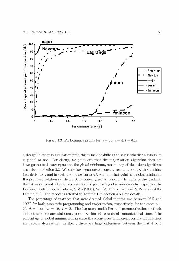
85


0

10

20

30

40

50

60

70

80

90

100

1 1.2 1.4 1.6 1.8 2 2.2

Performance ratio

Pe

rce

nta

ge

of

att

ain

ed

pe

rfo

rma

nc

e r

ati

o

Lagrange

Newton

major

param

fmincon

fmincon

Lagrange

param

major

Newton()

( )

Figure 3.3: Performance profile for n = 20, d = 4, t = 0.1s.

although in other minimization problems it may be difficult to assess whether a minimum

is global or not. For clarity, we point out that the majorization algorithm does not

have guaranteed convergence to the global minimum, nor do any of the other algorithms

described in Section 3.2. We only have guaranteed convergence to a point with vanishing

first derivative, and in such a point we can verify whether that point is a global minimum.

If a produced solution satisfied a strict convergence criterion on the norm of the gradient,

then it was checked whether such stationary point is a global minimum by inspecting the

Lagrange multipliers, see Zhang & Wu (2003), Wu (2003) and Grubisic & Pietersz (2005,

Lemma 6.1). The reader is referred to Lemma 1 in Section 4.5.4 for details.

The percentage of matrices that were deemed global minima was between 95% and

100% for both geometric programming and majorization, respectively, for the cases n =

20, d = 4 and n = 10, d = 2. The Lagrange multiplier and parametrization methods

did not produce any stationary points within 20 seconds of computational time. The

percentage of global minima is high since the eigenvalues of financial correlation matrices

are rapidly decreasing. In effect, there are large differences between the first 4 or 5

86


0

10

20

30

40

50

60

70

80

90

100

1 1.2 1.4 1.6 1.8 2 2.2

Performance ratio

Pe

rce

nta

ge

of

att

ain

ed

pe

rfo

rma

nc

e r

ati

o

Lagrange

Newton

major

param

fmincon

fmincon

Lagrange

param

major

Newton

()

( )

Figure 3.4: Performance profile for n = 80, d = 20, t = 2s.

consecutive eigenvalues. For the case n = 80, d = 20 it was more difficult to check

the global minimum criterion since subsequent eigenvalues are smaller and closer to each

other. In contrast, if we apply the methods for all cases to random correlation matrices

of Davies & Higham (2000), for which the eigenvalues are all very similar, we find that a

much lower percentage of produced stationary points were global minima.

3.5.2 Non-constant weights

We considered the example with non-constant weights described in Rebonato (2002, Sec-

tion 9.3), in which a functional form for the correlation matrix is specified, that is,

ρij = LongCorr + (1− LongCorr) exp− β|ti − tj|

, i, j = 1, . . . , n.

The parameters are set to n = 10, LongCorr = 0.6, β = 0.1, ti = i. Subsequently

Rebonato presents the rank 2, 3, and 4 matrices found by the parametrization method for

the case of equal weights. The majorization algorithm was also applied and its convergence

criterion was set to machine precision for the norm of the gradient. Comparative results

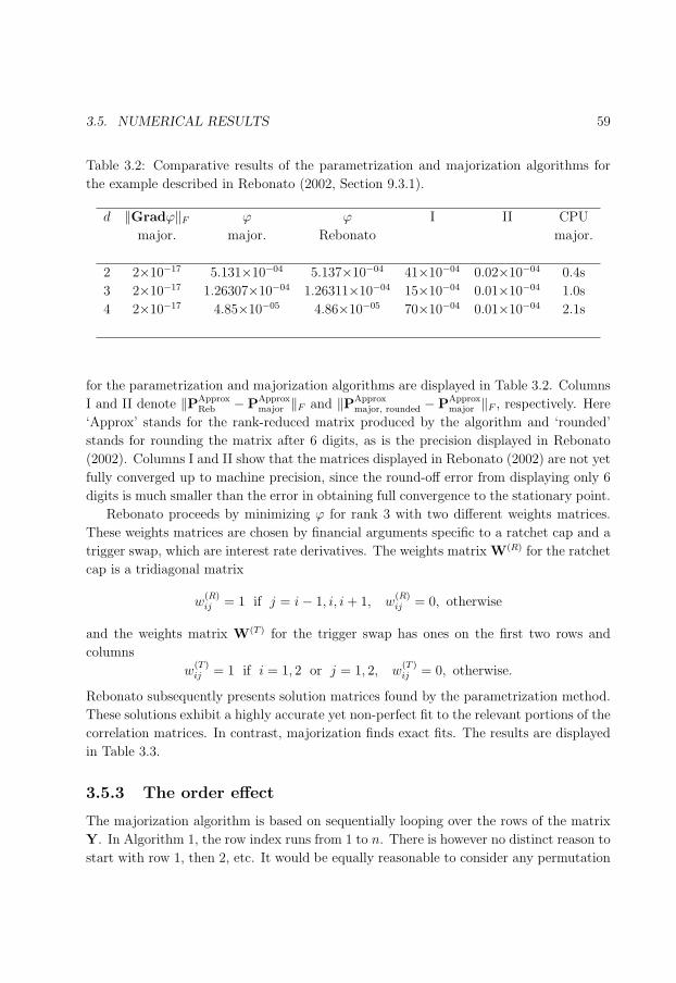
87


Table 3.2: Comparative results of the parametrization and majorization algorithms for

the example described in Rebonato (2002, Section 9.3.1).

d ‖Gradϕ‖F ϕ ϕ I II CPU

major. major. Rebonato major.

2 2×10−17 5.131×10−04 5.137×10−04 41×10−04 0.02×10−04 0.4s

3 2×10−17 1.26307×10−04 1.26311×10−04 15×10−04 0.01×10−04 1.0s

4 2×10−17 4.85×10−05 4.86×10−05 70×10−04 0.01×10−04 2.1s

for the parametrization and majorization algorithms are displayed in Table 3.2. Columns

I and II denote ‖PApproxReb −PApprox

major ‖F and ‖PApproxmajor, rounded −PApprox

major ‖F , respectively. Here

‘Approx’ stands for the rank-reduced matrix produced by the algorithm and ‘rounded’

stands for rounding the matrix after 6 digits, as is the precision displayed in Rebonato

(2002). Columns I and II show that the matrices displayed in Rebonato (2002) are not yet

fully converged up to machine precision, since the round-off error from displaying only 6

digits is much smaller than the error in obtaining full convergence to the stationary point.

Rebonato proceeds by minimizing ϕ for rank 3 with two different weights matrices.

These weights matrices are chosen by financial arguments specific to a ratchet cap and a

trigger swap, which are interest rate derivatives. The weights matrix W(R) for the ratchet

cap is a tridiagonal matrix

w(R)ij = 1 if j = i− 1, i, i + 1, w

(R)ij = 0, otherwise

and the weights matrix W(T ) for the trigger swap has ones on the first two rows and

columns

w(T )ij = 1 if i = 1, 2 or j = 1, 2, w

(T )ij = 0, otherwise.

Rebonato subsequently presents solution matrices found by the parametrization method.

These solutions exhibit a highly accurate yet non-perfect fit to the relevant portions of the

correlation matrices. In contrast, majorization finds exact fits. The results are displayed

in Table 3.3.

3.5.3 The order effect

The majorization algorithm is based on sequentially looping over the rows of the matrix

Y. In Algorithm 1, the row index runs from 1 to n. There is however no distinct reason to

start with row 1, then 2, etc. It would be equally reasonable to consider any permutation

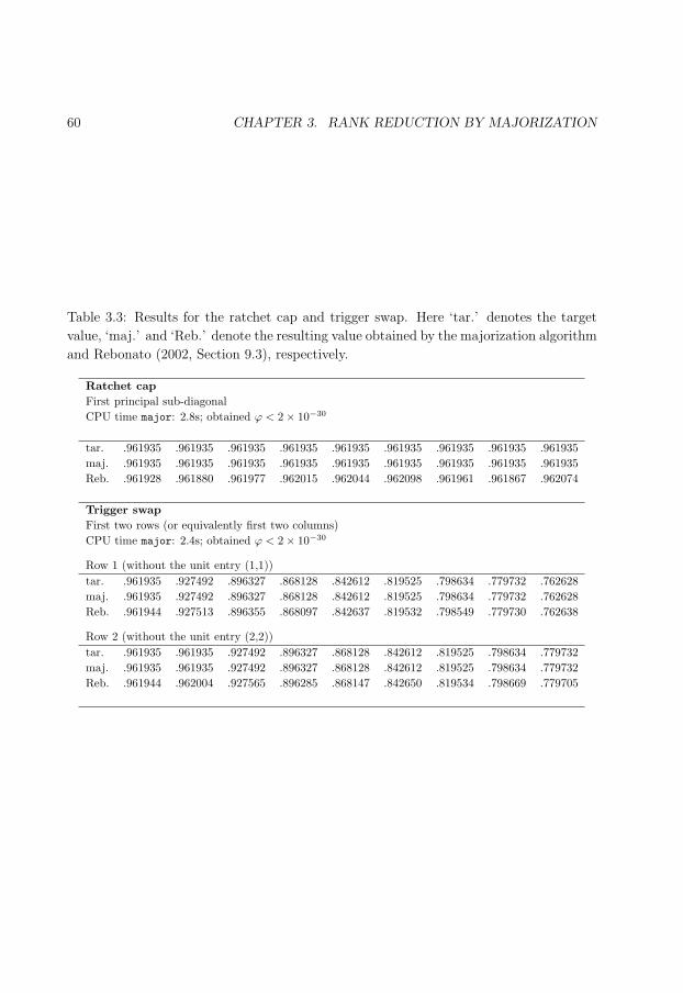
88


Table 3.3: Results for the ratchet cap and trigger swap. Here ‘tar.’ denotes the target

value, ‘maj.’ and ‘Reb.’ denote the resulting value obtained by the majorization algorithm

and Rebonato (2002, Section 9.3), respectively.

Ratchet capFirst principal sub-diagonalCPU time major: 2.8s; obtained ϕ < 2× 10−30

tar. .961935 .961935 .961935 .961935 .961935 .961935 .961935 .961935 .961935maj. .961935 .961935 .961935 .961935 .961935 .961935 .961935 .961935 .961935Reb. .961928 .961880 .961977 .962015 .962044 .962098 .961961 .961867 .962074

Trigger swapFirst two rows (or equivalently first two columns)CPU time major: 2.4s; obtained ϕ < 2× 10−30

Row 1 (without the unit entry (1,1))tar. .961935 .927492 .896327 .868128 .842612 .819525 .798634 .779732 .762628maj. .961935 .927492 .896327 .868128 .842612 .819525 .798634 .779732 .762628Reb. .961944 .927513 .896355 .868097 .842637 .819532 .798549 .779730 .762638

Row 2 (without the unit entry (2,2))tar. .961935 .961935 .927492 .896327 .868128 .842612 .819525 .798634 .779732maj. .961935 .961935 .927492 .896327 .868128 .842612 .819525 .798634 .779732Reb. .961944 .962004 .927565 .896285 .868147 .842650 .819534 .798669 .779705

89


p of the numbers 1, . . . , n and then let the row index run as p(1), p(2), . . . , p(n). A

priori, there is nothing to guarantee or prevent that the resulting solution point produced

with permutation p would differ from or be equal to the solution point produced by the

default loop 1, . . . , n. This dependency of the order is termed ‘the order effect’. The order

effect is a bad feature of Algorithm 1 in general. We show empirically that the solutions

produced by the algorithm can differ when using a different permutation. However, we

show that this is unlikely to happen for financial correlation matrices. The order effect

can have two consequences. First, the produced solution correlation matrix can differ –

this generally implies a different objective function value as well. Second, even when the

produced solution correlation matrix is equal, the configuration Y can differ – in this

case we have equal objective function values. To see this, consider a n× d configuration

matrix Y and assume given any orthogonal d × d matrix Q, that is, QQT = I. Then

the configuration matrices Y and YQ are associated with the same correlation matrices5:

YQQTY = YYT .

We investigated the order effect for Algorithm 1 numerically, as follows. We generated

either a random matrix by (3.15), see Section 3.5.1, or a random correlation matrix in

MATLAB by

rand(’state’,0);randn(’state’,0);n=30;R=gallery(’randcorr’,n);

The random correlation matrix generator gallery(’randcorr’,n) has been described

in Davies & Higham (2000). Subsequently we generated 100 random permutations with

p=randperm(n);. For each of the permutations, Algorithm 1 was applied with d = 2 and

a high accuracy was demanded: ε‖Gradϕ‖ = εϕ = 10−16. The results for the two different

correlation matrices are as follows.

(Random interest rate correlation matrix as in (3.15).) Only one type of produced

solution correlation matrix could be distinguished, which turned out to be a global min-

imum by inspection of the Lagrange multipliers. We also investigated the orthogonal

transformation effect. For R2, an orthogonal transformation can be characterized by the

rotation of the two basis vectors and then by -1 or +1 denoting whether the second basis

vector is reflected in the origin or not. All produced matrices Y were differently rotated,

but no reflection occurred. The maximum rotation was equal to 0.8 degrees and the

standard deviation of the rotation was 0.2 degrees.

(Davies & Higham (2000) random correlation matrix.) Essentially four types of pro-

duced solution correlation matrices could be distinguished, which we shall name I, II, III,

and IV. The associated objective function values and the frequency at which the types

occurred are displayed in Table 3.4. We inspected the Lagrange multipliers to find that

5The indeterminacy of the result produced by the algorithm can easily be resolved by either consideringonly YYT or by rotation of Y into its principal axes. For the latter, let YT Y = QΛQT be an eigenvaluedecomposition. Then the principal axes representation is given by YQ.

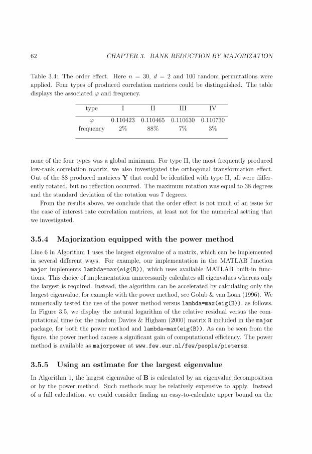
90


Table 3.4: The order effect. Here n = 30, d = 2 and 100 random permutations were

applied. Four types of produced correlation matrices could be distinguished. The table

displays the associated ϕ and frequency.

type I II III IV

ϕ 0.110423 0.110465 0.110630 0.110730

frequency 2% 88% 7% 3%

none of the four types was a global minimum. For type II, the most frequently produced

low-rank correlation matrix, we also investigated the orthogonal transformation effect.

Out of the 88 produced matrices Y that could be identified with type II, all were differ-

ently rotated, but no reflection occurred. The maximum rotation was equal to 38 degrees

and the standard deviation of the rotation was 7 degrees.

From the results above, we conclude that the order effect is not much of an issue for

the case of interest rate correlation matrices, at least not for the numerical setting that

we investigated.

3.5.4 Majorization equipped with the power method

Line 6 in Algorithm 1 uses the largest eigenvalue of a matrix, which can be implemented

in several different ways. For example, our implementation in the MATLAB function

major implements lambda=max(eig(B)), which uses available MATLAB built-in func-

tions. This choice of implementation unnecessarily calculates all eigenvalues whereas only

the largest is required. Instead, the algorithm can be accelerated by calculating only the

largest eigenvalue, for example with the power method, see Golub & van Loan (1996). We

numerically tested the use of the power method versus lambda=max(eig(B)), as follows.

In Figure 3.5, we display the natural logarithm of the relative residual versus the com-

putational time for the random Davies & Higham (2000) matrix R included in the major

package, for both the power method and lambda=max(eig(B)). As can be seen from the

figure, the power method causes a significant gain of computational efficiency. The power

method is available as majorpower at www.few.eur.nl/few/people/pietersz.

3.5.5 Using an estimate for the largest eigenvalue

In Algorithm 1, the largest eigenvalue of B is calculated by an eigenvalue decomposition

or by the power method. Such methods may be relatively expensive to apply. Instead

of a full calculation, we could consider finding an easy-to-calculate upper bound on the

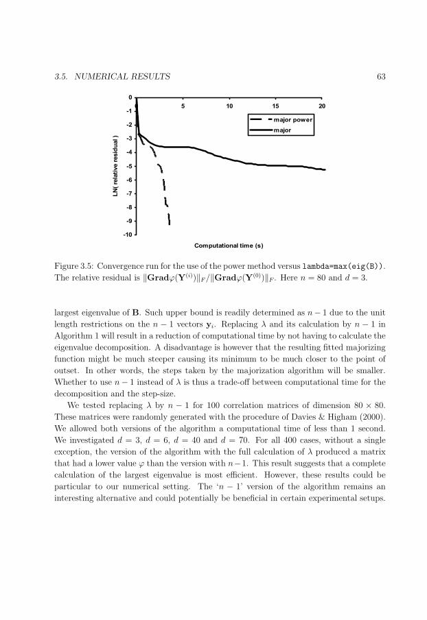
91


-10

-9

-8

-7

-6

-5

-4

-3

-2

-1

0

0 5 10 15 20

Computational time (s)

LN

( re

lati

ve r

esid

ual )

major power

major

Figure 3.5: Convergence run for the use of the power method versus lambda=max(eig(B)).

The relative residual is ‖Gradϕ(Y(i))‖F /‖Gradϕ(Y(0))‖F . Here n = 80 and d = 3.

largest eigenvalue of B. Such upper bound is readily determined as n− 1 due to the unit

length restrictions on the n − 1 vectors yi. Replacing λ and its calculation by n − 1 in

Algorithm 1 will result in a reduction of computational time by not having to calculate the

eigenvalue decomposition. A disadvantage is however that the resulting fitted majorizing

function might be much steeper causing its minimum to be much closer to the point of

outset. In other words, the steps taken by the majorization algorithm will be smaller.

Whether to use n− 1 instead of λ is thus a trade-off between computational time for the

decomposition and the step-size.

We tested replacing λ by n − 1 for 100 correlation matrices of dimension 80 × 80.

These matrices were randomly generated with the procedure of Davies & Higham (2000).

We allowed both versions of the algorithm a computational time of less than 1 second.

We investigated d = 3, d = 6, d = 40 and d = 70. For all 400 cases, without a single

exception, the version of the algorithm with the full calculation of λ produced a matrix

that had a lower value ϕ than the version with n−1. This result suggests that a complete

calculation of the largest eigenvalue is most efficient. However, these results could be

particular to our numerical setting. The ‘n − 1’ version of the algorithm remains an

interesting alternative and could potentially be beneficial in certain experimental setups.

92


3.6 Conclusions

We have developed a novel algorithm for finding a low-rank correlation matrix locally

nearest to a given matrix. The algorithm is based on iterative majorization and this

chapter is the first to apply majorization to the area of derivatives pricing. We showed

theoretically that the algorithm converges to a stationary point from any starting point.

As an addition to the previously available methods in the literature, majorization was

in our simulation setup more efficient than either geometric programming, the Lagrange

multiplier technique or the parametrization method. Furthermore, majorization is easier

to implement than any method other than modified PCA. The majorization method

efficiently and straightforwardly allows for arbitrary weights.

3.A Appendix: Proof of Equation (3.13)

Define the Algorithm 1 mapping y(k+1)i = mi(y

(k)i ,Y(k)). For ease of exposition we sup-

press the dependency on the row index i and current state Y(k), so y(k+1) = m(y(k)),

with

m(y) =z

‖z‖ , z = (λI−B)y + a,

where B depends on Y according to (3.9), λ is the largest eigenvalue of B and a =∑j:i6=j wijρijyj. We have locally around y(∞), by first order Taylor approximation

y(k+1) = y(∞) + Dm(y(∞))(y(k) − y(∞)

)+O

( ∥∥∥y(k) − y(∞)∥∥∥

2)

.

By straightforward calculation, the Jacobian matrix equals

Dm(y(∞)) =(

I− (y(∞)

)(y(∞)

)T) 1

‖z(∞)‖(λI−B).

The matrix I − (y(∞))(y(∞))T is denoted by Py(∞) . Then, up to first order in δ(k) =

‖y(k) − y(∞)‖,

y(k+1) − y(∞) ≈ Py(∞)

1

‖z(∞)‖(λI−B)(y(k) − y(∞)

)

= Py(∞)

1

‖z(∞)‖(

(λI−B)y(k) + a− ((λI−B)y(∞) + a

) )

= Py(∞)

1

‖z(∞)‖(z(k) − z(∞)

)

=‖z(k)‖‖z(∞)‖Py(∞)

(y(k) − y(∞)

), (3.16)

93

3.A. APPENDIX: PROOF OF EQUATION (3.11) 65

Figure 3.6: The equality ‖Py(∞)(y(k) − y(∞))‖ = δ(k)√

1− (δ(k))2/4.

where in the last equality we have used Py(∞)y(∞) = 0. We note that, up to first order in

δ(k), ‖z(k)‖/‖z(∞)‖ ≈ 1. The term ‖Py(∞)(y(k) − y(∞))‖ can be calculated by elementary

geometry, see Figure 3.6. The projection operator Py(∞) sets any component in the

direction of y(∞) to zero and leaves any orthogonal component unaltered. The resulting

length ‖Py(∞)(y(k)−y(∞))‖ has been illustrated in Figure 3.6. If we denote this length by

µ, then µ = sin(θ), where θ is the angle as denoted in the figure. Also sin(θ/2) = δ(k)/2

from which we obtain θ = 2 arcsin(δ(k)/2). It follows that

µ = sin(

2 arcsin(δ(k)/2

) )

= 2 sin(

arcsin(δ(k)/2

) )cos

(arcsin

(δ(k)/2

) )

= 2

(δ(k)

2

)√1−

(δ(k)

2

)2

= δ(k)

√1− (

δ(k))2

/4 = δ(k) +O( (δ(k)

)2 ). (3.17)

The result δ(k+1) = δ(k) +O((δ(k))2) follows by combining (3.16) and (3.17). 2

94

95

Chapter 4

Rank reduction of correlation

matrices by geometric programming

Geometric optimisation algorithms are developed that efficiently find the nearest low-rank

correlation matrix. We show, in numerical tests, that our methods compare favourably

to the existing methods in the literature. The connection with the Lagrange multiplier

method is established, along with an identification of whether a local minimum is a global

minimum. An additional benefit of the geometric approach is that any weighted norm

can be applied. The problem of finding the nearest low-rank correlation matrix occurs as

part of the calibration of multi-factor interest rate market models to correlation.

4.1 Introduction

The problem of finding the nearest low-rank correlation matrix occurs in areas such as

finance, chemistry, physics and image processing. The mathematical formulation of this

problem is stated in (3.4), in terms of the configuration matrix Y. Here, we state the

problem in terms of correlation matrices. Let Sn denote the set of real symmetric n × n

matrices and let P be a symmetric n×n matrix with unit diagonal. For C ∈ Sn we denote

by C º 0 that C is positive semidefinite. Let the desired rank d ∈ 1, . . . , n be given.

The problem is then given by

Find C ∈ Sn

to minimize 12‖P−C‖2

subject to rank(C) ≤ d; cii = 1, i = 1, . . . , n; C º 0.

(4.1)

Here ‖ · ‖ denotes a semi-norm on Sn. The most important instance is

1

2‖P−C‖2 =

1

2

∑i<j

wij(ρij − cij)2, (4.2)

96

68 CHAPTER 4. RANK REDUCTION BY GEOMETRIC PROGRAMMING

where W is a weights matrix consisting of non-negative elements. In words: Find the

low-rank correlation matrix C nearest to the given n×n matrix P. The choice of the

semi-norm will reflect what is meant by nearness of the two matrices. The semi-norm in

(4.2) is well known in the literature, and it is called the Hadamard semi-norm, see Horn &

Johnson (1990). We note that the constraint set is non-convex for d < n, which makes it

not straightforward to solve Problem (4.1) with standard convex optimization methods.

For concreteness, consider the following example. Suppose P is

1.0000 −0.1980 −0.3827

−0.1980 1.0000 −0.2416

−0.3827 −0.2416 1.0000

,

and W is the full matrix, wij = 1. With the algorithm developed in this chapter, we solve

(4.1) with P as above and d = 2. The algorithm takes as initial input a matrix C(0) of

rank 2 or less, for example,

C(0) =

1.0000 0.9782 0.8982

0.9782 1.0000 0.9699

0.8982 0.9699 1.0000

,

and then produces a sequence of points on the constraint set that converges to the point

C∗ =

1.0000 −0.4068 −0.6277

−0.4068 1.0000 −0.4559

−0.6277 −0.4559 1.0000

that solves (4.1). The constraint set and the points generated by the algorithm are

represented in Figure 4.1. The details of this representation are given in Section 4.5.2.

The blue point in the center and the green point represent, respectively, the target matrix

P and the solution point C∗. As the figure suggests, the algorithm has fast convergence

and the constraint set is a curved space.

This novel technique we propose, is based on geometric optimisation that can locally

minimize the objective function in (4.1) and which incorporates the Hadamard semi-norm.

In fact, our method can be applied to any sufficiently smooth objective function. Not all

other methods available in the literature that aim to solve (4.1) can handle an arbitrary

objective function, see the literature review in Section 3.2. We formulate the problem in

terms of Riemannian geometry. This approach allows us to use numerical methods on

manifolds that are numerically stable and efficient, in particular the Riemannian-Newton

method is applied. We show, for the numerical tests we performed, that the numerical

efficiency of geometric optimisation compares favourably to the other algorithms available

in the literature. The only drawback of the practical use of geometric optimisation is that

97


Figure 4.1: The shell represents the set of 3×3 correlation matrices of rank 2 or less. The

details of this representation are given in Section 4.5.2.

the implementation is rather involved. To overcome this drawback, we have made available

a MATLAB implementation ‘LRCM min’ (low-rank correlation matrices minimization)

at www.few.eur.nl/few/people/pietersz.

We develop a technique to instantly check whether an obtained local minimum is a

global minimum, by adaptation of Lagrange multiplier results of Zhang & Wu (2003).

The novelty consists of an expression for the Lagrange multipliers given the matrix C,

whereas until now only the reverse direction (an expression for the matrix C given the

Lagrange multipliers) was known. The fact that one may instantly identify whether a

local minimum is a global minimum is very rare for non-convex optimisation problems,

and that makes Problem (4.1), which is non-convex for d < n, all the more interesting.

Problem (4.1) is important in finance, as it occurs as part of the calibration of the

multi-factor LIBOR market model of Brace et al. (1997), Miltersen et al. (1997), Jamshid-

ian (1997) and Musiela & Rutkowski (1997). This model is an interest rate derivatives

pricing model, as explained in Section 1.3.2, and it is used in some financial institutions

for valuation and risk management of their interest rate derivatives portfolio. The num-

ber of stochastic factors needed for the model to fit to the given correlation matrix is

equal to the rank of the correlation matrix. This rank can be as high as the number of

forward LIBORs in the model, i.e., as high as the dimension of the matrix. The number

98


of LIBORs in the model can grow large in practical applications, for example, a model

with over 80 LIBORs is not uncommon. This implies that the number of factors needed

to fit the model to the given correlation matrix can be high, too. There is much empirical

evidence that the term structure of interest rates is driven by multiple factors (three, four,

or even more), see the review article of Dai & Singleton (2003). Though the number of

factors driving the term structure may be four or more, the empirical work shows that it

is certainly not as high as, say, 80. This is one reason for using a model with a low number

of factors. Another reason is the enhanced efficiency when estimating the model-price of

an interest rate derivative through Monte Carlo simulation. First, a lower factor model

simply requires drawing less random numbers than a higher factor model. Second, the

complexity of calculating LIBOR rates over a single time step in a simulation implemen-

tation is of order n × d, with n the number of LIBORs and d the number of factors, see

Joshi (2003b).

The importance of Problem (4.1) in finance has been recognized by many researchers.

In fact, the literature review of Section 3.2 refers to twenty articles or books addressing

the problem.

Due to its generality our method finds locally optimal points for a variety of other ob-

jective functions subject to the same constraints. One of the most famous problems comes

from physics and is called Thomson’s problem. The Thomson problem is concerned with

minimizing the potential energy of n charged particles on the sphere in R3 (d = 3). Geo-

metric optimisation techniques have previously been applied to the Thomson problem by

Depczynski & Stockler (1998), but these authors have only considered conjugate gradient

techniques on a ‘bigger’ manifold, in which the freedom of rotation has not been fac-

tored out. In comparison, we stress here that our approach considers a lower dimensional

manifold, which allows for Newton’s algorithm (the latter not developed in Depczynski &

Stockler (1998)). An implementation of geometric optimisation applied to the Thomson

problem has also been included in the ‘LRCM min’ package.

Finally, for a literature review of interest rate models, the reader is referred to Rebon-

ato (2004a).

The chapter is organized as follows. In Section 4.2, the constraints of the problem

are formulated in terms of differential geometry. We parameterize the set of correlation

matrices of rank at most d with a manifold named the Cholesky manifold. This is a

canonical space for the optimisation of the arbitrary smooth function subject to the

same constraints. In Section 4.3, the Riemannian structure of the Cholesky manifold

is introduced. Formulas are given for parallel transport, geodesics, gradient and Hessian.

These are needed for the minimization algorithms, which are made explicit. In Section

4.4, we discuss the convergence of the algorithms. In Section 4.5, the application of the

algorithms to the problem of finding the nearest low-rank correlation matrix is worked out

99

4.2. SOLUTION METHODOLOGY WITH GEOMETRIC OPTIMISATION 71

in detail. In Section 4.6, we numerically investigate the algorithms in terms of efficiency.

Finally, in Section 4.7, we conclude the chapter.

For a literature review on rank reduction methods, the reader is referred to Section

3.2.

4.1.1 Weighted norms

We mention two reasons for assigning non-constant or non-homogeneous weights in the

objective function of (4.2). First, in our setting P has the interpretation of measured

correlation. It can thus be the case that we are more confident of specific entries of the

matrix P. Second, the weighted norm of (4.2) has important applications in finance, see,

for example, Higham (2002), Rebonato (1999c) and Pietersz & Groenen (2004b).

The semi-norm in the objective function ϕ can be (i) a Hadamard semi-norm with

arbitrary weights per element of the matrix, as defined in (4.2), or (ii) a weighted Frobenius

norm ‖ · ‖F,Ω with Ω a positive definite matrix. Here ‖X‖2F,Ω = tr(XΩXTΩ). The

weighted Frobenius norm is, from a practical point of view, by far less transparent than

the Hadamard or weights-per-entry semi-norm (4.2). The geometric optimisation theory

developed in this chapter, and most of the algorithms mentioned in Section 3.2, can be

efficiently applied to both cases. The Lagrange multipliers and alternating projections

methods however can only be efficiently extended to the case of the weighted Frobenius

norm. The reason is that both these methods need to calculate a projection onto the

space of matrices of rank d or less. Such a projection, for the weighted Frobenius norm,

can be efficiently found by an eigenvalue decomposition. For the Hadamard semi-norm,

such an efficient solution is not available, to our knowledge, and as also mentioned in

Higham (2002, page 336).

4.2 Solution methodology with geometric optimisa-

tion

We note that Problem (4.1) is a special case of the following more general problem:

Find C ∈ Sn

to minimize ϕ(C)

subject to rank(C) ≤ d; cii = 1, i = 1, . . . , n; C º 0.

(4.3)

In this chapter methods will be developed to solve Problem (4.3) for the case when ϕ is

twice continuously differentiable. In the remainder of the chapter, we assume d > 1, since

for d = 1 the constraint set consists of a finite number (2n−1) of points.

100


4.2.1 Basic idea

The idea for solving Problem (4.3) is to parameterize the constraint set by a manifold,

and subsequently utilize the recently developed algorithms for optimisation over mani-

folds, such as Newton’s algorithm and conjugate gradient algorithms. Such geometric

optimisation has been developed by Smith (1993).

In Section 4.2.2, the constraint set is equipped with a topology, and we make an

identification with a certain quotient space. In Section 4.2.3, it will be shown that the

constraint set as such is not a manifold; however a dense subset is shown to be a manifold,

namely the set of matrices of rank exactly d. Subsequently, in Section 4.2.4, we will define a

larger manifold (named Cholesky manifold), of the same dimension as the rank-d manifold,

that maps surjectively to the constraint set. We may apply geometric optimisation on

the Cholesky manifold. The connection between minima on the Cholesky manifold and

on the constraint set will be established.

4.2.2 Topological structure

In this section, the set of n×n correlation matrices of rank d or less is equipped with

the subspace topology from Sn. We subsequently establish a homeomorphism (i.e., a

topological isomorphism) between the latter topological space and the quotient space of n

products of the d−1 sphere over the group of orthogonal transformations of Rd. Intuitively

the correspondence is as follows: We can associate with an n×n correlation matrix of rank

d a configuration of n points of unit length in Rd such that the inner product of points i

and j is entry (i, j) of the correlation matrix. Any orthogonal rotation of the configuration

does not alter the associated correlation matrix. This idea is developed more rigorously

below.

Definition 1 The set of symmetric n×n correlation matrices of rank at most d is defined

by

Cn,d =

C ∈ Sn ; Diag(C) = I, rank(C) ≤ d, C º 0.

Here I denotes the identity matrix and Diag denotes the map Rn×n → Rn×n, Diag(C)ij =

δijcij, where δij denotes the Kronecker delta.

The set Cn,d is a subset of Sn. The latter space is equipped with the Frobenius norm

‖ · ‖F , which in turn defines a topology. We equip Cn,d with the subspace topology.

In the following, the product of n unit spheres Sd−1 is denoted by Tn,d. Elements of

Tn,d are denoted as a matrix Y ∈ Rn×d, with each row vector yi of unit length. Denote

by Od the group of orthogonal transformations of d-space. Elements of Od are denoted

by a d×d orthogonal matrix Q.

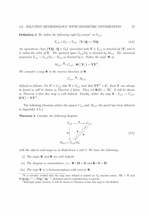
101


Definition 2 We define the following right Od-action1 on Tn,d:

Tn,d ×Od → Tn,d, (Y,Q) 7→ YQ. (4.4)

An equivalence class YQ : Q ∈ Od associated with Y ∈ Tn,d is denoted by [Y] and it

is called the orbit of Y. The quotient space Tn,d/Od is denoted by Mn,d. The canonical

projection Tn,d → Tn,d/Od = Mn,d is denoted by π. Define the map2 Ψ as

Mn,dΨ−→ Cn,d, Ψ

([Y]

)= YYT .

We consider a map Φ in the inverse direction of Ψ,

Cn,dΦ−→ Mn,d,

defined as follows: For C ∈ Cn,d take Y ∈ Tn,d such that YYT = C. Such Y can always

be found as will be shown in Theorem 2 below. Then set Φ(C) = [Y]. It will be shown

in Theorem 2 that this map is well defined. Finally, define the map S : Tn,d → Cn,d,

S(Y) = YYT .

The following theorem relates the spaces Cn,d and Mn,d; the proof has been deferred

to Appendix 4.A.1.

Theorem 2 Consider the following diagram

Tn,d Cn,d

Mn,d = Tn,d/Od

-S

?

Π

¡¡

¡¡

¡¡µΦ

¡¡

¡¡

¡¡ª

Ψ(4.5)

with the objects and maps as in Definitions 1 and 2. We have the following:

(i) The maps Ψ and Φ are well defined.

(ii) The diagram is commutative, i.e., Ψ Π = S and Φ S = Π.

(iii) The map Ψ is a homeomorphism with inverse Φ.

1It is trivially verified that the map thus defined is indeed an Od smooth action: YI = Y andY(Q1Q2)−1 = (YQ−1

2 )Q1−1. Standard matrix multiplication is smooth.

2Although rather obvious, it will be shown in Theorem 2 that this map is well defined.

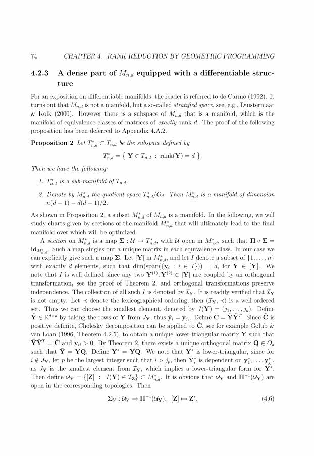
102


4.2.3 A dense part of Mn,d equipped with a differentiable struc-

ture

For an exposition on differentiable manifolds, the reader is referred to do Carmo (1992). It

turns out that Mn,d is not a manifold, but a so-called stratified space, see, e.g., Duistermaat

& Kolk (2000). However there is a subspace of Mn,d that is a manifold, which is the

manifold of equivalence classes of matrices of exactly rank d. The proof of the following

proposition has been deferred to Appendix 4.A.2.

Proposition 2 Let T ∗n,d ⊂ Tn,d be the subspace defined by

T ∗n,d =

Y ∈ Tn,d : rank(Y) = d

.

Then we have the following:

1. T ∗n,d is a sub-manifold of Tn,d.

2. Denote by M∗n,d the quotient space T ∗

n,d/Od. Then M∗n,d is a manifold of dimension

n(d− 1)− d(d− 1)/2.

As shown in Proposition 2, a subset M∗n,d of Mn,d is a manifold. In the following, we will

study charts given by sections of the manifold M∗n,d that will ultimately lead to the final

manifold over which will be optimized.

A section on M∗n,d is a map Σ : U → T ∗

n,d, with U open in M∗n,d, such that Π Σ =

idM∗n,d

. Such a map singles out a unique matrix in each equivalence class. In our case we

can explicitly give such a map Σ. Let [Y] in M∗n,d, and let I denote a subset of 1, . . . , n

with exactly d elements, such that dim(span(yi : i ∈ I)) = d, for Y ∈ [Y]. We

note that I is well defined since any two Y(1),Y(2) ∈ [Y] are coupled by an orthogonal

transformation, see the proof of Theorem 2, and orthogonal transformations preserve

independence. The collection of all such I is denoted by IY. It is readily verified that IY

is not empty. Let ≺ denote the lexicographical ordering, then (IY,≺) is a well-ordered

set. Thus we can choose the smallest element, denoted by J(Y) = (j1, . . . , jd). Define

Y ∈ Rd×d by taking the rows of Y from JY, thus yi = yji. Define C = YYT . Since C is

positive definite, Cholesky decomposition can be applied to C, see for example Golub &

van Loan (1996, Theorem 4.2.5), to obtain a unique lower-triangular matrix Y such that

YYT = C and yii > 0. By Theorem 2, there exists a unique orthogonal matrix Q ∈ Od

such that Y = YQ. Define Y∗ = YQ. We note that Y∗ is lower-triangular, since for

i /∈ JY, let p be the largest integer such that i > jp, then Y∗i is dependent on y∗1, . . . ,y

∗jp

,

as JY is the smallest element from IY, which implies a lower-triangular form for Y∗.Then define UY = [Z] : J(Y) ∈ IZ ⊂ M∗

n,d. It is obvious that UY and Π−1(UY) are

open in the corresponding topologies. Then

ΣY : UY → Π−1(UY), [Z] 7→ Z∗, (4.6)

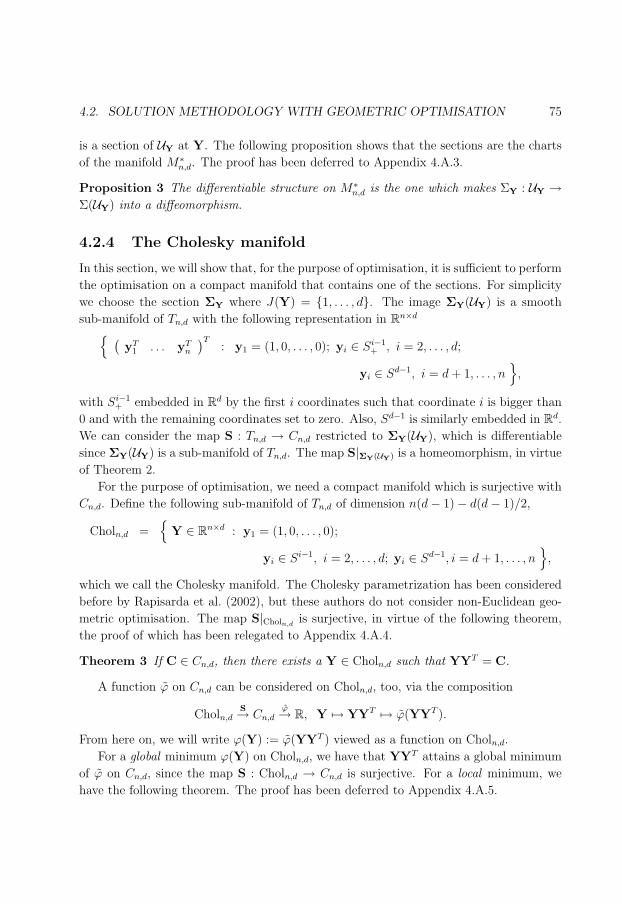
103


is a section of UY at Y. The following proposition shows that the sections are the charts

of the manifold M∗n,d. The proof has been deferred to Appendix 4.A.3.

Proposition 3 The differentiable structure on M∗n,d is the one which makes ΣY : UY →

Σ(UY) into a diffeomorphism.

4.2.4 The Cholesky manifold

In this section, we will show that, for the purpose of optimisation, it is sufficient to perform

the optimisation on a compact manifold that contains one of the sections. For simplicity

we choose the section ΣY where J(Y) = 1, . . . , d. The image ΣY(UY) is a smooth

sub-manifold of Tn,d with the following representation in Rn×d

(yT

1 . . . yTn

)T: y1 = (1, 0, . . . , 0); yi ∈ Si−1

+ , i = 2, . . . , d;

yi ∈ Sd−1, i = d + 1, . . . , n

,

with Si−1+ embedded in Rd by the first i coordinates such that coordinate i is bigger than

0 and with the remaining coordinates set to zero. Also, Sd−1 is similarly embedded in Rd.

We can consider the map S : Tn,d → Cn,d restricted to ΣY(UY), which is differentiable

since ΣY(UY) is a sub-manifold of Tn,d. The map S|ΣY(UY) is a homeomorphism, in virtue

of Theorem 2.

For the purpose of optimisation, we need a compact manifold which is surjective with

Cn,d. Define the following sub-manifold of Tn,d of dimension n(d− 1)− d(d− 1)/2,

Choln,d =

Y ∈ Rn×d : y1 = (1, 0, . . . , 0);

yi ∈ Si−1, i = 2, . . . , d; yi ∈ Sd−1, i = d + 1, . . . , n

,

which we call the Cholesky manifold. The Cholesky parametrization has been considered

before by Rapisarda et al. (2002), but these authors do not consider non-Euclidean geo-

metric optimisation. The map S|Choln,dis surjective, in virtue of the following theorem,

the proof of which has been relegated to Appendix 4.A.4.

Theorem 3 If C ∈ Cn,d, then there exists a Y ∈ Choln,d such that YYT = C.

A function ϕ on Cn,d can be considered on Choln,d, too, via the composition

Choln,dS→ Cn,d

ϕ→ R, Y 7→ YYT 7→ ϕ(YYT ).

From here on, we will write ϕ(Y) := ϕ(YYT ) viewed as a function on Choln,d.

For a global minimum ϕ(Y) on Choln,d, we have that YYT attains a global minimum

of ϕ on Cn,d, since the map S : Choln,d → Cn,d is surjective. For a local minimum, we

have the following theorem. The proof has been deferred to Appendix 4.A.5.

104


Theorem 4 The point Y attains a local minimum of ϕ on Choln,d if and only if YYT

attains a local minimum of ϕ on Cn,d.

These considerations on global and local minima on Choln,d show that, to optimize ϕ

over Cn,d, we might as well optimize ϕ over the manifold Choln,d. For the optimisation of

ϕ over Cn,d, there is no straightforward way to use numerical methods such as Newton and

conjugate gradient, since they require a notion of differentiability, but for optimisation of

ϕ on Choln,d, we can use such numerical methods.

4.2.5 Choice of representation

In principle, we could elect another manifold M and a surjective open map M → Cn,d.

We insist however on explicit knowledge of the geodesics and parallel transport, for this

is essential to obtaining an efficient algorithm. We found that if we choose the Cholesky

manifold then convenient expressions for geodesics, etc., are obtained. Moreover, the

Cholesky manifold has the minimal dimension, i.e., dim(Choln,d) = dim(M∗n,d).

In the next section, the geometric optimisation tools are developed for the Cholesky

manifold.

4.3 Optimisation over the Cholesky manifold

For the development of minimization algorithms on a manifold, certain objects of the

manifold need to calculated explicitly, such as geodesics, parallel transport, etc. In this

section, these objects are introduced and made explicit for Choln,d.

From a theoretical point of view, it does not matter which coordinates we choose to

derive the geometrical properties of a manifold. For the numerical computations however

this choice is essential because the simplicity of formulas for the geodesics and parallel

transport depends on the chosen coordinates. We found that simple expressions are

obtained when Choln,d is viewed as a sub-manifold of Tn,d, which, in turn, is viewed as a

subset of the ambient space Rn×d. This representation reveals that, to calculate geodesics

and parallel transport on Choln,d, it is sufficient to calculate these on a single sphere.

The tangent space of the manifold Choln,d at a point Y ∈ Choln,d is denoted by

TYCholn,d. A tangent vector at a point Y is an element of TYCholn,d and is denoted by

∆.

4.3.1 Riemannian structure

We start with a review of basic concepts of Riemannian geometry. Our exposition follows

do Carmo (1992). Let M be an m-dimensional differentiable manifold. A Riemannian

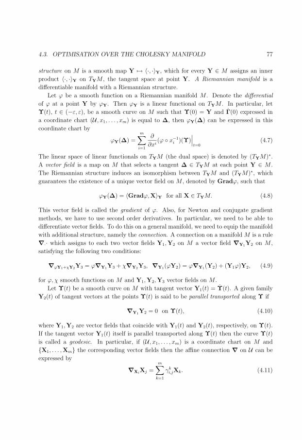
105

4.3. OPTIMISATION OVER THE CHOLESKY MANIFOLD 77

structure on M is a smooth map Y 7→ 〈·, ·〉Y, which for every Y ∈ M assigns an inner

product 〈·, ·〉Y on TYM , the tangent space at point Y. A Riemannian manifold is a

differentiable manifold with a Riemannian structure.

Let ϕ be a smooth function on a Riemannian manifold M . Denote the differential

of ϕ at a point Y by ϕY. Then ϕY is a linear functional on TYM . In particular, let

Υ(t), t ∈ (−ε, ε), be a smooth curve on M such that Υ(0) = Y and Γ(0) expressed in

a coordinate chart (U , x1, . . . , xm) is equal to ∆, then ϕY(∆) can be expressed in this

coordinate chart by

ϕY(∆) =m∑

i=1

∂

∂xi(ϕ x−1

i )(Υ)∣∣∣t=0

(4.7)

The linear space of linear functionals on TYM (the dual space) is denoted by (TYM)∗.A vector field is a map on M that selects a tangent ∆ ∈ TYM at each point Y ∈ M .

The Riemannian structure induces an isomorphism between TYM and (TYM)∗, which

guarantees the existence of a unique vector field on M , denoted by Gradϕ, such that

ϕY(∆) = 〈Gradϕ,X〉Y for all X ∈ TYM. (4.8)

This vector field is called the gradient of ϕ. Also, for Newton and conjugate gradient

methods, we have to use second order derivatives. In particular, we need to be able to

differentiate vector fields. To do this on a general manifold, we need to equip the manifold

with additional structure, namely the connection. A connection on a manifold M is a rule

∇·· which assigns to each two vector fields Y1,Y2 on M a vector field ∇Y1Y2 on M ,

satisfying the following two conditions:

∇ϕY1+χY2Y3 = ϕ∇Y1Y3 + χ∇Y2Y3, ∇Y1(ϕY2) = ϕ∇Y1(Y2) + (Y1ϕ)Y2, (4.9)

for ϕ, χ smooth functions on M and Y1,Y2,Y3 vector fields on M .

Let Υ(t) be a smooth curve on M with tangent vector Y1(t) = Υ(t). A given family

Y2(t) of tangent vectors at the points Υ(t) is said to be parallel transported along Υ if

∇Y1Y2 = 0 on Υ(t), (4.10)

where Y1,Y2 are vector fields that coincide with Y1(t) and Y2(t), respectively, on Υ(t).

If the tangent vector Y1(t) itself is parallel transported along Υ(t) then the curve Υ(t)

is called a geodesic. In particular, if (U , x1, . . . , xm) is a coordinate chart on M and

X1, . . . ,Xm the corresponding vector fields then the affine connection ∇ on U can be

expressed by

∇XiXj =

m∑

k=1

γki,jXk. (4.11)

106


The functions γki,j are smooth functions, called the Christoffel symbols for the connection.

In components, the geodesic equation becomes

xk +m∑

i,j=1

γki,jxixj = 0, (4.12)

where xk are the coordinates of Υ(t). On a Riemannian manifold there is a unique torsion

free connection compatible with the metric, called the Levi-Civita connection. This means

that Christoffel symbols can be expressed as functions of a metric on M . We note that

(4.12) implies as well that, once we have determined the equation for the geodesic, we can

simply read off Christoffel symbols. With respect to an induced metric the geodesic is

the curve of shortest length between two points on a manifold. For a manifold embedded

in Euclidean space an equivalent characterization of a geodesic is that the acceleration

vector at each point along a geodesic is normal to the manifold so long as the curve is

traced with uniform speed.

We start by defining Riemannian structures for Tn,d and for the Cholesky manifold

Choln,d. We use the Levi-Civita connection, associated to the metric defined as follows

on the tangent spaces. Both tangent spaces are identified with suitable subspaces of the

ambient space Rn×d, and subsequently the inner product for two tangents ∆1, ∆2 is

defined as

〈∆1,∆2〉 = tr∆1∆T2 , (4.13)

which is the Frobenius inner product for n × d matrices. We note that, in our special

case, the inner product 〈·, ·〉Y is independent of the point Y; therefore we suppress the

dependency on Y.

4.3.2 Normal and tangent spaces

An equation determining tangents to Tn,d at a point Y can be obtained by differentiating

Diag(YYT ) = I yielding Diag(Y∆T +∆YT ) = 0, i.e., Diag(∆YT ) = 0. The dimension

of the tangent space is n(d − 1). The normal space at the point Y is defined to be the

orthogonal complement of the tangent space at the point Y, i.e., it consists of the matrices

N, for which tr∆NT = 0 for all ∆ in the tangent space. It follows that the normal space is

n dimensional. It is straightforward to verify that if N = DY, where D is n×n diagonal,

then N is in the normal space. Since the dimension of the space of such matrices is n, we

see that the normal space NYTn,d at Y ∈ Tn,d is given by

NYTn,d =

DY ; D ∈ Rn×n diagonal.

The projections ΠNYTn,dand ΠTYTn,d

onto the normal and tangent spaces of Tn,d are given

by

ΠNYTn,d(∆) = Diag(∆YT )Y and ΠTYTn,d

(∆) = ∆−Diag(∆YT )Y,

107

4.3. OPTIMISATION OVER THE CHOLESKY MANIFOLD 79

respectively. The projection ΠTYCholn,donto the tangent space of Choln,d is given by

ΠTYCholn,d(∆) = Z

(ΠTYTn,d

(∆)),

with Z(∆) defined by

zij(∆) =

0 for j > i or i = j = 1,

δij otherwise.

4.3.3 Geodesics

It is convenient to work with the coordinates of the ambient space Rn×d. In this coordinate

system, geodesics on Tn,d with respect to the Levi-Civita connection obey the second order

differential equation

Y + ΓY(Y, Y) = 0, with ΓY(∆1,∆2) := Diag(∆1∆T2 )Y. (4.14)

To see this, we begin with the condition that Y(t) remains on Tn,d,

Diag(YYT ) = I. (4.15)

Differentiating this equation twice, we obtain,

Diag(YYT + 2YYT + YYT ) = 0. (4.16)

In order for Y(·) to be a geodesic, Y(t) must be in the normal space at Y(t), i.e.,

Y(t) = D(t)Y(t) (4.17)

for some diagonal matrix D(t). To obtain an expression for D, substitute (4.17) into

(4.16), which yields (4.14).

The function ΓY is the matrix notation of the Christoffel symbols, γkij, with respect

to E1, . . . ,End, the standard basis vectors of Rn×d. More precisely, ∇EiEj =

∑ndk=1 γk

ijEk

with γkij defined by

〈ΓY(X1,X2),Ek〉 =nd∑

i,j=1

γkij(X1)i(X2)j.

The geodesic at Y(0) ∈ Tn,d in the direction ∆ ∈ TY(0)Tn,d is given by,

Yi(t) = cos( ‖∆i‖t)Yi(0) +

1

‖∆i‖ sin( ‖∆i‖t

)∆i. (4.18)

for i = 1, . . . , n, per component on the sphere. By differentiating, we obtain an expression

for the evolution of the tangent along the geodesic:

Yi(t) = −‖∆i‖ sin( ‖∆i‖t

)Yi(0) + cos

( ‖∆i‖t)∆i. (4.19)

Since Choln,d is a Riemannian sub-manifold of Tn,d it has the same geodesics.

108


4.3.4 Parallel transport along a geodesic

We consider this problem per component on the sphere. If ∆(2) ∈ TY(1)Tn,d is parallel

transported along a geodesic starting from Y(1) in the direction of ∆(1) ∈ TY(1)Tn,d, then

decompose ∆(2) in terms of ∆(1),

∆(2)i (t) = 〈∆(1)

i (0),∆(2)i (0)〉∆(1)

i (t) + Ri, Ri⊥∆(1)i (0).

Then ∆(1)i (t) changes according to (4.19) and Ri remains unchanged. Parallel transport

from Y(1) to Y(2) defines an isometry T(Y(1),Y(2)) : TY(1)Tn,d → TY(2)Tn,d. When it is

clear in between which two points is transported, then parallel transport is denoted simply

by T. Since Choln,d is a Riemannian sub-manifold of Tn,d it has the same equations for

parallel transport.

4.3.5 The gradient

Since Choln,d is a sub-manifold of Rn×d we can use coordinates of Rn×d to express the

differential ϕY of ϕ at the point Y, namely (ϕY)ij = ∂F∂Yij

. The gradient Gradϕ of a

function ϕ on Choln,d can be determined by (4.8). It follows that,

Gradϕ = ΠTYCholn,d(ϕY) = Z

(ϕY −Diag(ϕYYT )Y

). (4.20)

4.3.6 Hessian

The Hessian Hessϕ of a function ϕ is a second covariant derivative of ϕ. More precisely,

let ∆1,∆2 be two vector fields, then

Hessϕ(∆1,∆2) = 〈∇∆1Gradϕ,∆2〉

In local coordinates of Rn×d

Hessϕ(∆1,∆2) = ϕYY(∆1,∆2)− 〈ϕY, ΓY(∆1,∆2)〉, (4.21)

where

ϕYY(∆1,∆2) =d

dt

d

ds

∣∣∣∣t=s=0

ϕ(Y(t, s)), withd

dt

∣∣∣∣t=0

Y = ∆1,d

ds

∣∣∣∣s=0

Y = ∆2.

Newton’s method requires inverting the Hessian at minus the gradient, therefore we need

to find the tangent ∆ to Choln,d such that

Hessϕ(∆,X) = 〈−Gradϕ,X〉, for all tangents X to Choln,d. (4.22)

109

4.4. DISCUSSION OF CONVERGENCE PROPERTIES 81

To solve (4.22), it is convenient to calculate the unique tangent vector H = H(∆) satis-

fying

Hessϕ(∆,X) = 〈H,X〉, for all tangents X to Choln,d,

since then the Newton Equation (4.22) becomes H(∆) = −Gradϕ. From (4.14) and

(4.21), we obtain

H(∆) = ΠTYCholn,d(ϕYY(∆))−Diag(ϕYYT )∆, (4.23)

where the notation ϕYY(∆) means the tangent vector satisfying

ϕYY(∆) =d

dt

∣∣∣∣t=0

ϕY(Y(t)), Y(0) = ∆.

4.3.7 Algorithms

We are now in a position to state the conjugate gradient algorithm, given as Algorithm

2, and the Newton algorithm, given as Algorithm 3, for optimisation over the Cholesky

manifold. These algorithms are instances of the geometric programs presented in Smith

(1993), for the particular case of the Cholesky manifold.

4.4 Discussion of convergence properties

In this section, we discuss convergence properties of the geometric programs: global con-

vergence and the local rate of convergence.

4.4.1 Global convergence

First, we discuss global convergence for the Riemannian-Newton algorithm. It is well

known that the Newton algorithm, as displayed in Algorithm 3, is not globally convergent

to a local minimum. Moreover, the steps in Algorithm 3 may even not be well defined,

because the Hessian mapping could be singular. The standard way to resolve these issues,

is to introduce jointly a steepest descent algorithm. So Algorithm 3 is adjusted in the

following way. When the new search direction ∆(k) has been calculated, then we also

consider the steepest descent search direction ∆(k)Steep = −Gradϕ(Y(k)). Subsequently, a

line minimization of the objective value is performed in both directions, ∆(k) and ∆(k)Steep.

We then take as the next point of the algorithm whichever search direction finds the point

with lowest objective value. Such a steepest descent method with line minimization is

well known to have guaranteed convergence to a local minimum.

Second, we discuss global convergence for conjugate gradient algorithms. For the

Riemannian case, we have not seen any global convergence results for conjugate gradient

110


Algorithm 2 Conjugate gradient for minimizing ϕ(Y) on Choln,d

Input: Y(0), ϕ(·).Require: Y(0) such that Y(0)(Y(0))T = I.

Compute G(0) = Gradϕ(Y(0)) = Z(ϕY − Diag(ϕY(Y(0))T )Y(0)) and set J(0) =

−G(0).

for k = 0, 1, 2, ... do

Minimize ϕ(Y(k)(t)

)over t where Y(k)(t) is a geodesic on Choln,d starting from

Y(k) in the direction of J(k).

Set tk = tmin and Y(k+1) = Y(k)(tk).

Compute G(k+1) = Gradϕ(Y(k+1)) = Z(

ϕY −Diag(ϕY(Y(k+1))T )Y(k+1)).

Parallel transport tangent vectors J(k) and G(k) to the point Y(k+1).

Compute the new search direction

J(k+1) = −G(k+1)+γkTJ(k) where

γk = 〈G(k+1)−TG(k),G(k+1)〉〈G(k),G(k)〉 , Polak-Ribiere,

γk = ||G(k+1)||2||G(k)||2 , Fletcher-Reeves.

Reset J(k+1) = −G(k+1) if k + 1 ≡ 0 mod n(d− 1)− 12d(d− 1).

end for

Algorithm 3 Newton’s method for minimizing ϕ(Y) on Choln,d.

Input: Y(0), ϕ(·).Require: Y(0) such that Diag(Y(0)(Y(0))T ) = I.

for k = 0, 1, 2, ... do

Compute G(k) = Gradϕ(Y(k)) = Z(

ϕY −Diag(ϕYYT )Y).

Compute ∆(k) = −H−1G(k), i.e. ∆(k) ∈ TYCholn,d and

Z(

ϕYY(∆(k))−Diag(

ϕYY(∆(k))(Y(k))T)Y(k)

)

−Diag(ϕY(Y(k))T )∆(k) = −G(k).

Move from Y(k) in direction ∆(k) to Y(k)(1) along the geodesic.

Set Y(k+1) = Y(k)(1).

end for

111

4.4. DISCUSSION OF CONVERGENCE PROPERTIES 83

algorithms in the literature. Therefore we focus on the results obtained for the flat-

Euclidean case. Zoutendijk (1970) and Al-Baali (1985) establish global convergence of

the Fletcher & Reeves (1964) conjugate gradient method with line minimization. Gilbert

& Nocedal (1992) establish alternative line search minimizations that guarantee global

convergence of the Polak & Ribiere (1969) conjugate gradient method.

4.4.2 Local rate of convergence

Local rates of convergence for geometric optimisation algorithms are established in Smith

(1993), Edelman, Arias & Smith (1999) and Dedieu, Priouret & Malajovich (2003).

In Theorem 3.3 of Smith (1993), the following result is established for the Riemannian-

Newton method. If Y is a non-degenerate stationary point, then there exists an open set

U containing Y, such that starting from any Y(0) in U , the sequence of points produced

by Algorithm 3 converges quadratically to Y.

In Theorem 4.3 of Smith (1993), the following result is stated for the Riemannian

Fletcher & Reeves (1964) and Polak & Ribiere (1969) conjugate gradient methods. Sup-

pose Y is a non-degenerate stationary point such that the Hessian at Y is positive definite.

Suppose Y(j)∞j=0 is a sequence of points, generated by Algorithm 2, converging to Y.

Then, for sufficiently large j, the sequence Y(j)∞j=0 has dim(Choln,d)-steps quadratic

convergence to Y.

As a numerical illustration, convergence runs are displayed in Figure 4.2, for reducing

a 10× 10 correlation matrix to rank 3. The following algorithms are compared:

1. Steepest descent, for which the search direction J(k+1) in Algorithm 2 is equal to

−G(k+1), i.e., to minus the gradient. The steepest descent method has a linear local

rate of convergence, see Smith (1993, Theorem 2.3).

2. PRCG, Polak-Ribiere conjugate gradient.

3. FRCG, Fletcher-Reeves conjugate gradient.

4. Newton.

5. Lev.-Mar., the Levenberg (1944) & Marquardt (1963) method, which is a Newton-

type method.

The code that is used for this test is the package ‘LRCM min’, to be discussed in Section

4.6. This package also contains the correlation matrix used for the convergence run test.

Figure 4.2 clearly illustrates the convergence properties of the various geometric programs.

The efficiency of the algorithms is studied in Section 4.6 below.

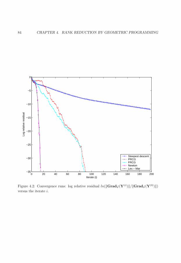
112


0 20 40 60 80 100 120 140 160 180 200−35

−30

−25

−20

−15

−10

−5

0

Iterate (i)

Log

rela

tive

resi

dual

Steepest descentPRCGFRCGNewtonLev.− Mar

Figure 4.2: Convergence runs: log relative residual ln(‖Gradϕ(Y(i))‖/‖Gradϕ(Y(0))‖)versus the iterate i.

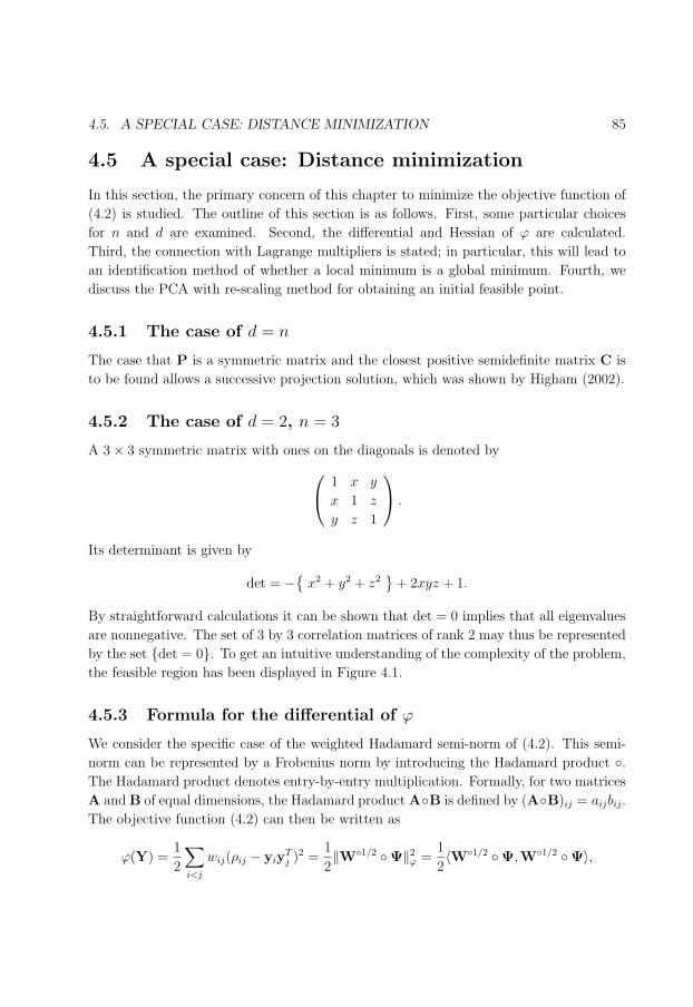
113

4.5. A SPECIAL CASE: DISTANCE MINIMIZATION 85

4.5 A special case: Distance minimization

In this section, the primary concern of this chapter to minimize the objective function of

(4.2) is studied. The outline of this section is as follows. First, some particular choices

for n and d are examined. Second, the differential and Hessian of ϕ are calculated.

Third, the connection with Lagrange multipliers is stated; in particular, this will lead to

an identification method of whether a local minimum is a global minimum. Fourth, we

discuss the PCA with re-scaling method for obtaining an initial feasible point.

4.5.1 The case of d = n

The case that P is a symmetric matrix and the closest positive semidefinite matrix C is

to be found allows a successive projection solution, which was shown by Higham (2002).

4.5.2 The case of d = 2, n = 3

A 3× 3 symmetric matrix with ones on the diagonals is denoted by

1 x y

x 1 z

y z 1

.

Its determinant is given by

det = −x2 + y2 + z2

+ 2xyz + 1.

By straightforward calculations it can be shown that det = 0 implies that all eigenvalues

are nonnegative. The set of 3 by 3 correlation matrices of rank 2 may thus be represented

by the set det = 0. To get an intuitive understanding of the complexity of the problem,

the feasible region has been displayed in Figure 4.1.

4.5.3 Formula for the differential of ϕ

We consider the specific case of the weighted Hadamard semi-norm of (4.2). This semi-

norm can be represented by a Frobenius norm by introducing the Hadamard product .The Hadamard product denotes entry-by-entry multiplication. Formally, for two matrices

A and B of equal dimensions, the Hadamard product AB is defined by (AB)ij = aijbij.

The objective function (4.2) can then be written as

ϕ(Y) =1

2

∑i<j

wij(ρij − yiyTj )2 =

1

2‖W1/2 Ψ‖2

ϕ =1

2〈W1/2 Ψ,W1/2 Ψ〉,

114


with Ψ := YYT −P and with (W1/2)ij =√

wij. Then

d

dtϕ(Y(t)) = 〈W1/2 Ψ,W1/2 Ψ〉 = 〈Ψ,W Ψ〉

= 〈∆YT + Y∆T ,W Ψ〉= 〈∆YT ,W Ψ〉+ 〈Y∆T ,W Ψ〉= 〈∆, 2(W Ψ)Y〉 = 〈∆, ϕY〉, ∀∆.

Thus from (4.7) we have

ϕY = 2(W Ψ)Y. (4.24)

Similarly, we may compute the second derivative

ϕYY(∆) =d

dt

∣∣∣t=0

ϕY(Y(t)) = 2((W Ψ)∆ +

(W (∆YT + Y∆T )

)Y

),

with Y(·) any curve starting from Y in the direction of ∆.

4.5.4 Connection normal with Lagrange multipliers

The following lemma provides the basis for the connection of the normal vector at Y versus

the Lagrange multipliers of the algorithm of Zhang & Wu (2003) and Wu (2003). The

result is novel since previously only an expression was known for the matrix Y given the

Lagrange multipliers. The result below establishes the reverse direction. This Lagrange

result will allow us to identify whether a local minimum is also a global minimum. That

we are able to efficiently determine whether a local minimum is a global minimum, is a

very rare phenomenon in non-convex optimisation, and makes the rank reduction problem

(non-convex for d < n) all the more interesting.

We note that the Lagrange theory is based on an efficient expression of the low-rank

projection by an eigenvalue decomposition. Therefore the theory below can be extended

efficiently only for the Hadamard norm with equal weights and for the weighted Frobenius

norm, see also the discussion in Section 4.1.1. The proof of the following lemma has been

deferred to Appendix 4.A.6.

Lemma 1 Let Y ∈ Tn,d be such that Gradϕ(Y) = 0. Here, Gradϕ is the gradient of ϕ

on Tn,d, Gradϕ(Y) = ΠTYTn,d(ϕY) = ϕY −Diag(ϕYYT )Y, with ϕY in (4.24). Define

λ :=1

2diag

(ϕYYT

)

and define P(λ) := P + Diag(λ). Then there exist a joint eigenvalue decomposition

P(λ) = QDQT , YYT = QD∗QT

where D∗ can be obtained by selecting at most d nonnegative entries from D (here if an

entry is selected it retains the corresponding position in the matrix).

115


The characterization of the global minimum for Problem (4.1) was first achieved in

Zhang & Wu (2003) and Wu (2003), which we repeat here: Denote by Cd a matrix

obtained by eigenvalue decomposition of C together with leaving in only the d largest

eigenvalues (in absolute value). Denote for λ ∈ Rn: P(λ) = P + Diag(λ). The proof of

the following theorem has been repeated for clarity in Appendix 4.A.7.

Theorem 5 (Characterization of the global minimum of Problem (4.1), see Zhang & Wu

(2003) and Wu (2003)) Let P be a symmetric matrix. Let λ∗ be such that there exists

P + Diag(λ∗)d ∈ Cn,d with

Diag( P + Diag(λ∗)d

)= Diag(P). (4.25)

Then P + Diag(λ∗)d is a global minimizer of Problem (4.1).

This brings us in a position to identify whether a local minimum is a global minimum:

Theorem 6 Let Y ∈ Tn,d be such that Gradϕ(Y) = 0 on Tn,d. Let λ and P(λ) be

defined as in Lemma 1. If YYT has the d largest eigenvalues from P(λ) (in absolute

value) then YYT is a global minimizer to the Problem (4.1).

PROOF: Apply Lemma 1 and Theorem 5. 2

4.5.5 Initial feasible point

To obtain an initial feasible point Y ∈ Tn,d we use the modified PCA method described

in Section 3.2.1. To obtain an initial feasible point in Choln,d, we perform a Cholesky

decomposition as in the proof of Theorem 3.

We note that the condition in Section 3.2.1 of decreasing norm of the eigenvalues is

thus key to ensure that the initial point is close to the global minimum, see the result of

Theorem 6.


There are many different algorithms available in the literature, as detailed in Section 3.2.

Some of these have an efficient implementation, i.e., the cost of a single iteration is low.

Some algorithms have fast convergence, for example, the Newton method has quadratic

convergence. Algorithms with fast convergence usually require less iterations to attain

a predefined convergence criterion. Thus, the real-world performance of an algorithm

is a trade-off between cost-per-iterate and number of iterations required. A priori, it is

not clear which algorithm will perform best. Therefore, in this section, the numerical

performance of geometric optimisation is compared to other methods available in the

literature.

116


4.6.1 Acknowledgement

Our implementation of geometric optimisation over low-rank correlation matrices ‘LRCM

min’3 is an adoption of the ‘SG min’ template of Edelman & Lippert (2000) (written in

MATLAB) for optimisation over the Stiefel and Grassmann manifolds. This template

contains four distinct well-known non-linear optimisation algorithms adapted for geomet-

ric optimisation over Riemannian manifolds: Newton algorithm; dogleg step or Levenberg

(1944) and Marquardt (1963) algorithm; Polak & Ribiere (1969) conjugate gradient; and

Fletcher & Reeves (1964) conjugate gradient.

4.6.2 Numerical comparison

The performances of the following seven algorithms, all of these described in Sections 4.3

and 3.2, except for item 7 (fmincon), are compared:

1. Geometric optimisation, Newton (Newton).

2. Geometric optimisation, Fletcher-Reeves conjugate gradient (FRCG).

3. Majorization, e.g., Pietersz & Groenen (2004b) (Chapter 3) (Major.).

4. Parametrization, e.g., Rebonato (1999b) (Param.).

5. Alternating projections without normal vector correction, e.g., Grubisic (2002)

(Alt. Proj.).

6. Lagrange multipliers, e.g., Zhang & Wu (2003) (Lagrange).

7. fmincon, a MATLAB built-in medium-scale constrained nonlinear program (fmin-

con).

We note that the first two algorithms in this list have been developed in this chapter. The

algorithms are tested on a large number (one hundred) of randomly generated correlation

matrices. The benefit of testing on many correlation matrices is, that the overall and

generic performance of the algorithms may be assessed. The random financial correlation

matrices are generated as described in Section 3.5.1.

As the benchmark criterion for the performance of an algorithm, we take its obtained

accuracy of fit given a fixed amount of computational time. Such a criterion corresponds

to financial practice, since decisions based on derivative valuation calculations often need

to be made within seconds. To display the comparison results, we use the state-of-the-art

and convenient performance profiles ; see Dolan & More (2002). The reader is referred

3LRCM min can be downloaded from www.few.eur.nl/few/people/pietersz.

117


1 1.01 1.02 1.03 1.04 1.05 1.06 1.07 1.080

10

20

30

40

50

60

70

80

90

100

Performance ratio ξ

Pre

form

ance

of a

ttain

ed p

erfo

rman

ce r

atio

Ω

Param.

Alt. Proj.

Lagrange

fmincon

Major.

Newton FRCG

NewtonFRCGMajor.Param.Alt. Proj.Lagrangefmincon

Figure 4.3: Performance profile with n = 30, d = 3, 2 seconds of computational time,

Hadamard norm with equal weights. A rule of thumb is, that the higher the graph of an

algorithm, the better its performance.

there for details, but the idea is described briefly in Section 3.5.1. A rule of thumb is,

that the higher the profile of an algorithm, the better its performance. The performance

profiles are displayed in Figures 4.3–4.6, for various choices of n, d, and computational

times. Each performance profile represents a benchmark on 100 different test interest rate

correlation matrices. For Figures 4.3–4.5, an objective function with equal weights is used.

For Figure 4.6, we use a Hadamard semi-norm with non-constant weights. These weights

are chosen so as to reflect the importance of the correlation entries for a specific trigger

swap, as outlined in, e.g., Rebonato (2004b, Section 20.4.3). For this specific trigger swap,

the first three rows and columns are important. Therefore the weights matrix W takes

the form

wij =

1 if i ≤ 3 or j ≤ 3,

0 otherwise.

From Figures 4.3–4.6 it becomes clear that geometric optimisation compares favoura-

bly to the other methods available in the literature, with respect to obtaining the best fit

to the original correlation matrix within a limited computational time.

118


1 1.1 1.2 1.3 1.4 1.50

10

20

30

40

50

60

70

80

90

100


Pre

form

ance

of a

ttain

ed p

erfo

rman

ce r

atio

Ω

Param.

Alt. Proj.

Lagrange

fmincon

Major.

Newton

FRCG


Figure 4.4: Performance profile with n = 50, d = 4, 1 second of computational time,

Hadamard norm with equal weights.

4.7 Conclusions

We applied geometric optimisation tools for finding the nearest low-rank correlation ma-

trix. The differential geometric machinery provided us with an algorithm more efficient

than any existing algorithm in the literature, at least for the numerical cases consid-

ered. The geometric approach also allows for insight and more intuition into the problem.

We established a technique that allows one to straightforwardly identify whether a local

minimum is a global minimum.

4.A Appendix: Proofs

4.A.1 Proof of Theorem 2

PROOF of (i). The maps Ψ and Φ are well defined: To show that Ψ is well defined, we

need to show that if Y2 ∈ [Y1], then Y2YT2 = Y1Y

T1 . From the assumption, we have

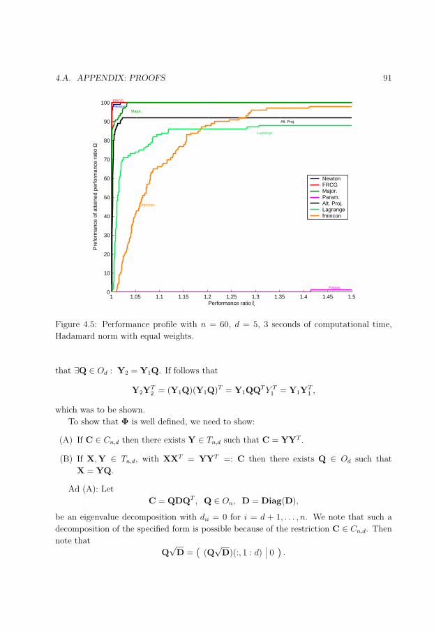
119

4.A. APPENDIX: PROOFS 91

1 1.05 1.1 1.15 1.2 1.25 1.3 1.35 1.4 1.45 1.50

10

20

30

40

50

60

70

80

90

100


Pre

form

ance

of a

ttain

ed p

erfo

rman

ce r

atio

Ω

Param.

Alt. Proj.

Lagrange

fmincon

Major. Newton

FRCG


Figure 4.5: Performance profile with n = 60, d = 5, 3 seconds of computational time,

Hadamard norm with equal weights.

that ∃Q ∈ Od : Y2 = Y1Q. If follows that

Y2YT2 = (Y1Q)(Y1Q)T = Y1QQT Y T

1 = Y1YT1 ,

which was to be shown.

To show that Φ is well defined, we need to show:

(A) If C ∈ Cn,d then there exists Y ∈ Tn,d such that C = YYT .

(B) If X,Y ∈ Tn,d, with XXT = YYT =: C then there exists Q ∈ Od such that

X = YQ.

Ad (A): Let

C = QDQT , Q ∈ On, D = Diag(D),

be an eigenvalue decomposition with dii = 0 for i = d + 1, . . . , n. We note that such a

decomposition of the specified form is possible because of the restriction C ∈ Cn,d. Then

note that

Q√

D =(

(Q√

D)(:, 1 : d) 0).

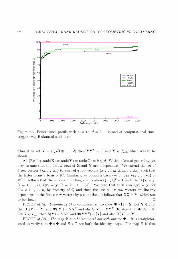
120


1 1.002 1.004 1.006 1.008 1.01 1.012 1.014 1.016 1.0180

10

20

30

40

50

60

70

80

90

100


Pre

form

ance

of a

ttain

ed p

erfo

rman

ce r

atio

Ω

Param.

fmincon

Major.

Newton

FRCG

NewtonFRCGMajor.Param.fmincon

Figure 4.6: Performance profile with n = 15, d = 3, 1 second of computational time,

trigger swap Hadamard semi-norm.

Thus if we set Y = (Q√

D)(:, 1 : d) then YYT = C and Y ∈ Tn,d, which was to be

shown.

Ad (B): Let rank(X) = rank(Y) = rank(C) = k ≤ d. Without loss of generality, we

may assume that the first k rows of X and Y are independent. We extend the set of

k row vectors x1, . . . ,xk to a set of d row vectors x1, . . . ,xk, xk+1, . . . , xd, such that

the latter forms a basis of Rd. Similarly, we obtain a basis y1, . . . ,yk, yk+1, . . . , yd of

Rd. It follows that there exists an orthogonal rotation Q, QQT = I, such that Qxi = yi

(i = 1, . . . , k), Qxi = yi (i = k + 1, . . . , d). We note that then also Qxi = yi for

i = k + 1, . . . , n, by linearity of Q and since the last n − k row vectors are linearly

dependent on the first k row vectors by assumption. It follows that XQ = Y, which was

to be shown. 2

PROOF of (ii). Diagram (4.5) is commutative: To show Ψ Π = S: Let Y ∈ Tn,d,

then Π(Y) = [Y] and Ψ([Y]) = YYT and also S(Y) = YYT . To show that Φ S = Π:

Let Y ∈ Tn,d, then S(Y) = YYT and Φ(YYT ) = [Y] and also Π(Y) = [Y]. 2

PROOF of (iii). The map Ψ is a homeomorphism with inverse Φ: It is straightfor-

ward to verify that Φ Ψ and Ψ Φ are both the identity maps. The map Ψ is thus

121


bijective with inverse Φ. To show that Ψ is continuous, note that for quotient spaces

we have: The map Ψ is continuous if and only if Ψ Π is continuous (see for exam-

ple Abraham, Marsden & Ratiu (1988), Proposition 1.4.8). In our case, Ψ Π = S

with S(Y) = YYT is continuous. The proof now follows from a well-known lemma

from topology: A continuous bijection from a compact space into a Hausdorff space is a

homeomorphism (see for example Munkres (1975), Theorem 5.6). 2

4.A.2 Proof of Proposition 2

1. It is sufficient to show that Y ∈ Rn×d : rank(Y) = d is open in Rn×d, since

T ∗n,d is open in Tn,d if and only if Y ∈ Rn×d : rank(Y) = d is open in Rn×d.

Since the rank of a symmetric matrix is a locally constant function, it follows that

Y ∈ Rn×d : rank(Y) = d = S−1(rank−1(d)) is an open subset of Rn×d, with

S(Y) = YYT as in Definition 2. 2

2. This part is a corollary of Theorem 1.11.4 of Duistermaat & Kolk (2000). This

theorem essentially states that for a smooth action of a Lie group on a manifold

the quotient is a manifold if the action is proper and free. First, we show that the

action of Od on T ∗n,d is proper4. Let

Ξ : T ∗n,d ×Od → T ∗

n,d × T ∗n,d, (Y,Q) 7→ (YQ,Y)

and K a compact subset of T ∗n,d × T ∗

n,d. We have to show that Ξ−1(K) is compact.

By continuity of Ξ, Ξ−1(K) is closed in T ∗n,d ×Od. Because T ∗

n,d ×Od is bounded it

follows that Ξ−1(K) is compact.

Second, we show that the Od-action on T ∗n,d is free. Let Y ∈ T ∗

n,d and Q ∈ Od such

that YQ = Y. Since rank(Y) = d, it follows from the proof of Theorem 2 (i) that

there exists precisely one Q ∈ Od such that YQ = Y. Thus, this Q must be the

identity matrix.

The dimension of M∗n,d = dim(T ∗

n,d)− dim(Od) = n(d− 1)− 12d(d− 1). 2

4.A.3 Proof of Proposition 3

This part is a corollary of Theorem 1.11.4 of Duistermaat & Kolk (2000). This theorem

states that there is only one differentiable structure on the orbit space which satisfies the

following: Suppose that, for every [Y] ∈ M∗n,d, we have an open neighbourhood U ⊆ M∗

n,d

and a bijective map:

U : Π−1(U) → U ×Od, Y 7→ (Π(Y),V(Y)),

4For a definition, see Duistermaat & Kolk (2000, page 53).

122


such that, for every Y ∈ Π−1(U), Q ∈ Od, U(YQ) = (Π(Y),V(Y)Q). The differentiable

structure on M∗n,d is the one which makes U into a diffeomorphism. The topology of M∗

n,d

obtained in this manner is equal to the quotient topology.

Let Y ∈ T ∗n,d and ΣY be a section over UY defined in (4.6). We define UY :

Π−1(UY) → UY×Od as follows. For Z ∈ Π−1([Z]), [Z] ∈ UY, there is a unique element

QZ ∈ Od such that Z = ΣY([Z])QZ. Then we define UY by UY(Z) = ([Z],QZ). By

definition, we have that U−1Y ([Z],Q) = ΣY([Z])Q. Since U−1

Y : Π−1(UY) → UY×Od is a

bijective map, we have that UY is bijective, too. It can be easily verified that UY satisfies

the condition UY(YQ) = ([Y],QYQ) of Theorem 1.11.4 of Duistermaat & Kolk (2000)

stated above. It follows that UY is a diffeomorphism if and only if ΣY : U → ΣY(U)

is a diffeomorphism. Thus, the differentiable structure on M∗n,d is the one which makes

ΣY : UY → Σ(UY) into a diffeomorphism. 2


Let C ∈ Cn,d and suppose that rank(C) = k ≤ d. Then there is a Y ∈ Tn,k such that

YYT = C, by Theorem 2. Apply to Y the procedure5 outlined in Section 4.2.3, to obtain

a lower-triangular matrix Y∗ ∈ Tn,k, such that Y∗(Y∗)T = C. A lower-triangular matrix

Y ∈ Choln,d that satisfies YYT = C can now easily be obtained by setting

Y =

(Y∗ 0︸︷︷︸

n×(d−k)

),

which was to be shown. 2


First, we prove the ‘only if’ part. We note that it is sufficient to show that the map

S : Choln,d → Cn,d is open. For then if Y attains a local minimum of ϕ on the open

neighbourhood U ⊂ Choln,d, then S(Y) = YYT attains a local minimum of ϕ on the open

neighbourhood S(U) of YYT , since for any C′ = Y′Y′T ∈ S(U), ϕ(C′) = ϕ(Y′Y′T ) =

ϕ(Y′) ≥ ϕ(Y) = ϕ(YYT ).

To show that S : Choln,d → Cn,d is open, note that it is sufficient to show that

Π : Choln,d → Mn,d is open, since Ψ : Mn,d → Cn,d is a homeomorphism (see Proposition

2, item 3) and S = Ψ Π.

Suppose, then, that U is open in Choln,d. We have to show that Π−1(Π(U)) is open

in Tn,d, by definition of the quotient topology of Mn,d. We have

Π−1(

Π(U))

=

YQ : Y ∈ U , Q ∈ Od

.

5The procedure in Section 4.2.3 is stated in terms of d, but k should be read there in this case.

123


It is sufficient to show that the complement (Π−1(Π(U)))c is closed. Let Y(i) be a

sequence in (Π−1(Π(U)))c converging to Y, i.e. limi→∞ ‖Y(i) −Y‖ = 0. We can write

Y(i) = Z(i)Q(i) with Z(i) ∈ U c and Q(i) ∈ Od. Then,

limi→∞

‖Y(i) −Y‖ = limi→∞

‖Z(i)Q(i) −Y‖ = limi→∞

‖Z(i) −Y(Q(i))T‖ = 0. (4.26)

Since U c × Od is compact, there exists a convergent subsequence (Z(ij),Q(ij)), with

Z(ij) → Z∗ ∈ U c and Q(ij) → Q∗, say. From (4.26) it follows that Z∗ = Y(Q∗)T ∈ U c,

which implies Y ∈ (Π−1(Π(U)))c.

The reverse direction is obvious since the map S : Choln,d → Cn,d is continuous. 2

4.A.6 Proof of Lemma 1

It is recalled from matrix analysis that C1 and C2 admit a joint eigenvalue decomposition

if and only if their Lie bracket [C1,C2] = C1C2 − C2C1 equals zero. Define P(λ) :=

−Ψ + Diag(λ). We note that 2Diag(λ)Y is the projection ΠNYTn,d(ϕY) of ϕY onto the

normal space at Y. We note also that

YYT + P(λ) = P(λ). (4.27)

We calculate

P(λ)Y =−Ψ + Diag(λ)

Y = −1

2ϕY +

1

2ΠNYTn,d

(ϕY

)= 0. (4.28)

The last equality follows from the assumption that Gradϕ(Y) = 0, i.e. the differential

ϕY is normal at Y. (Here, Gradϕ(Y) denotes the gradient on Tn,d.) It follows from

(4.28) and from the symmetry of P(λ) that

(i) YYT P(λ) = 0 and also,

(ii) [YYT , P(λ)] = 0.

From (ii), YYT and P(λ) admit a joint eigenvalue decomposition, but then also jointly

with P(λ) because of (4.27). Suppose P(λ) = QDQT . From (i) we then have that d∗ii and

dii cannot both be non-zero. The result now follows since YYT is positive semidefinite

and has rank less than or equal to d. 2


Define the Lagrangian

`(C, λ) := −‖P−C‖2ϕ − 2λTdiag(P−C), and

124


v(λ) := min

`(C,λ) : rank(C) = d. (4.29)

We note that the minimization problem in (4.29) is attained by any P(λ)d (see e.g.,

Equation (30) of Wu (2003)). For any C ∈ Cn,d,

‖P−C‖2F

(a)= −`(C,λ∗)

(b)

≥ −v(λ∗)(c)= ‖P− P(λ)d‖2

F .

(This is the equation at the end of the proof of Theorem 4.4 of Zhang & Wu (2003).)

Here (in-)equality

(a) is obtained from the property that C ∈ Cn,d,

(b) is by definition of v, and

(c) is by assumption of (4.25). 2

125

Chapter 5

Fast drift-approximated pricing in

the BGM model

1 It is demonstrated that the forward rates process discretized by a single time step

together with a separability assumption on the volatility function allows for representation

by a low-dimensional Markov process. This in turn leads to efficient pricing by, for

example, finite differences. We then develop a discretization based on the Brownian bridge

that is especially designed to have high accuracy for single time stepping. The scheme

is proven to converge weakly with order one. We compare the single time step method

for pricing on a grid with multi-step Monte Carlo simulation for a Bermudan swaption,

reporting a computational speed increase by a factor 10, yet maintaining sufficiently

accurate pricing.

5.1 Introduction

The BGM framework, developed by Brace et al. (1997), Miltersen et al. (1997) and

Jamshidian (1997), is now one of the most popular models for pricing interest rate deriva-

tives. In the BGM framework almost all prices are computed using Monte Carlo simula-

tion. An advantage of Monte Carlo is its applicability to almost any product. However, it

has the drawback of being computationally rather slow. In an attempt to limit the com-

putational time, Hunter et al. (2001), Jackel (2002, Section 12.5) and Kurbanmuradov,

Sabelfeld & Schoenmakers (2002) introduced predictor-corrector drift approximations,

which reduce the Monte Carlo stage to single time-step simulation.

1This chapter has been published in different form as Pietersz, R., Pelsser, A. A. J. & van Regenmortel,M. (2004), ‘Fast drift-approximated pricing in the BGM model’, Journal of Computational Finance8(1), 93–124. An extended abstract of this chapter appeared as Pietersz, R., Pelsser, A. A. J. & vanRegenmortel, M. (2005), ‘Bridging Brownian LIBOR’, Wilmott Magazine 18, 98–103.

126

98 CHAPTER 5. FAST DRIFT-APPROXIMATED PRICING FOR BGM

This chapter presents a significant addition to the single time step pricing method. We

show that much more efficient numerical methods (either numerical integration or finite

differences) may be used at the cost of a minor additional assumption, separability. The

latter is a non-restrictive requirement on the form of the volatility function. The single

time step together with separability renders the state of the BGM model completely

determined by a low-dimensional Markov process. This enables efficient implementation.

We give an example of the fast single time step pricing framework for Bermudan

swaptions. A comparison is made with prices obtained by least-squares multi-time step

Monte Carlo simulation in the BGM model. This includes the use of the Longstaff &

Schwartz (2001) method.

The computational speed increase achieved with the use of finite differences for BGM

single time step pricing is the main result. This chapter also contains two other results:

• The first result is a new time discretization using a Brownian bridge, as introduced

in Section 5.3, which is proven to have least-squares error in a certain sense (to be

defined) for single time step discretizations. In Section 5.5 it is shown numerically

that the Brownian bridge scheme outperforms (in the case of single time steps)

various other discretizations for the LIBOR-in-arrears density test. In the first part

of Section 5.6, we prove theoretically that the Brownian bridge scheme converges

weakly with order one when used for multi-time step Monte Carlo. In the second

part of Section 5.6, we compare the Brownian bridge scheme numerically with other

discretizations for multi-time steps.

• The second result is a method for measuring the accuracy of single time stepping.

This is the timing inconsistency test as outlined in Section 5.9.

A further application of the Brownian bridge drift approximation is its use in the likelihood

ratio method. This method, introduced by Broadie & Glasserman (1996), efficiently

estimates risk sensitivities for Monte Carlo pricing. The particular application of the

likelihood ratio method to the LIBOR market model has been developed by Glasserman

& Zhao (1999), who proposed the use of drift approximations.

The outline of this chapter is as follows. After setting out some basic notation and the

most important formulas for the BGM model, the single time step pricing framework is

developed, various discretization schemes are discussed and the Brownian bridge scheme

is introduced. The Brownian bridge scheme is then investigated theoretically and numer-

ically for both single and multi-time steps, respectively. Next, the proposed framework

is worked out for the one-factor case. This is followed by an example of the pricing of

Bermudan swaptions, both for a one- and a two-factor model. A test is then developed

to assess the quality of single time steps. Finally, conclusions are drawn.

127

5.2. NOTATION FOR BGM MODEL 99

5.2 Notation for BGM model

In this section our notation of the BGM model is introduced.

We consider a BGM model, M2 Such a model features n forward rates, fi, i = 1, . . . , n,

where forward i accrues from time ti to time ti+1, 0 < t1 < · · · < tn+1. Denote by αi

the accrual factor over the period [ti, ti+1]. Denote by bi(t) the time-t price of a discount

bond that expires at time ti. Bond prices and forward rates are linked by the relation

1 + αifi(t) =bi(t)

bi+1(t).

Each forward rate is driven by a d-dimensional Brownian motion (where d is the number

of stochastic factors in the BGM model), w, as follows:

dfi(t)

fi(t)= µi(t)dt + σi(t) · dw(t). (5.1)

Here σi is the d-dimensional volatility vector, and µi is the drift term, whose form will

in general depend on the choice of probability measure. Throughout this chapter, we use

the numeraire probability measure associated with the bond maturing at time tn+1, the

so called terminal measure. There is a specific reason why we use the terminal measure,

and this is explained in Remark 2 of Section 5.3. For the terminal measure, the drift term

will have the following form for i < n:

µi(t, fi+1, . . . , fn) = −n∑

k=i+1

αkfkσk(t) · σi(t)

1 + αkfk

. (5.2)

For i = n the drift term is zero. This simply expresses the well-known fact that a forward

rate is a martingale under its associated forward measure.

For the remainder of this chapter it will be useful to have stochastic differential equa-

tion (SDE) (5.1) in logarithmic form:

d log fi(t) = µi(t)dt + σi(t) · dw(n+1)(t), (5.3)

µi(t) = µi(t)− 1

2‖σi(t)‖2.

Last, we introduce the notion of all available forward rates at a given point in time.

Define i(t) to be the smallest integer i such that t ≤ ti. Define f to consist of all forward

rates that have not yet expired at time t, i.e.,

f(t) =(fi(t)(t), . . . , fn(t)

). (5.4)

2The construction of such a model may be found in, e.g., Musiela & Rutkowski (1997), Pelsser (2000)or Brigo & Mercurio (2001).

128


5.3 Single time step method for pricing on a grid

The two key elements in the development of a method to price interest rate derivatives

in the BGM model by low-dimensional finite differences are:

• the forward rates process should be discretized by a single time step scheme; and

• the volatility structure should be separable, which permits the dynamics of the single

time step forward rates process to be represented by a low-dimensional Markov

process.

5.3.1 Justification of the above assumptions

Because the forward rates are approximated by a single-step scheme, the model will in

general no longer be arbitrage-free. This timing inconsistency is addressed in Section 5.9,

where it is shown that its impact is negligible for most cases. The single-step approxi-

mation is accurate enough for the pricing of derivatives, as shown numerically in Section

5.8. At the end of this section we introduce a novel discretization scheme based on the

Brownian bridge that is especially designed for single time stepping. Its superiority (for

single time steps only) over other discretizations is established in Section 5.5.

We proceed by first introducing notation for the single step-approximated forward

rates process. This is followed by a statement of the separability assumption, after which

we establish the low-dimensional Markov representation result. Single time step dis-

cretizations are then discussed, and we end by considering methods for pricing American

style options with Monte Carlo methods.

5.3.2 Notation

We assume as given a time discretization τ0 < · · · < τm, m ≥ 1. A single time step

discretization is a discretization with m = 1. Define zi(u, v) =∫ v

uσi(t) · dw(n+1)(t).

Given a scheme for the log rates

log fi(τj+1) = log fi(τj) + µi

(τj, τj+1, f(τj), z(τj, τj+1)

)+ zi(τj, τj+1) (5.5)

then denote by

fAi (t) = fi(0) exp

µi

(0, t, f(0), z(0, t)

)+ zi(0, t)

its single time step-approximated equivalent. Here µ is the “drift approximation” and it

is determined by the scheme applied, which may be the Euler, the predictor-corrector or

the Brownian bridge scheme. These schemes will be elaborated on in Section 5.4. The A

in fA stands for “approximated”. The vector z is defined by analogy with f in (5.4).

129

5.3. SINGLE TIME STEP METHOD FOR PRICING ON A GRID 101

5.3.3 Separability

Definition 3 (Separability) A collection of volatility functions σi : [0, ti] → Rd, i =

1, . . . , n, is called “separable” if there exists a vector-valued function σ : [0, tn] → Rd and

vectors vi ∈ Rd, i = 1, . . . , n, such that

σi(t) = viσ(t) (5.6)

(no vector product; entry-by-entry multiplication) for 0 ≤ t ≤ ti, i = 1, . . . , n.

Separability appears regularly in the context of requiring a process to be Markov. We men-

tion three examples. First, we mention Ritchken & Sankarasubramanian (1995, Proposi-

tion 2.1). Working in the HJM model (Heath, Jarrow & Morton 1992), they show that

separability is a necessary and sufficient condition on the volatility structure such that

the dynamics of the term structure may be represented by a two-dimensional Markov

process. Second, we mention the Wiener chaos expansion framework of Hughston &

Rafailidis (2005). In this framework any interest rate model is completely characterized

by its so-called Wiener chaos expansion. The nth chaos expansion is represented by a

function φn : Rn+ → R that satisfies certain integrability conditions. If all φn are separable,

the resulting interest rate model turns out to be Markov. Third, we mention the finite-

dimensional Markov realizations for stochastic volatility forward rate models (see Bjork,

Landen & Svensson (2004)). Here a necessary condition for a stochastic volatility model

to have a finite-dimensional Markov realization is that the drift term and each component

of the volatility term in the Stratonovich representation of the short rate SDE should be a

sum of functions that are separable in time to expiry and the stochastic volatility driver.

We give an example of a separable volatility function in the case of a one-factor model

(d = 1).

Example 1 (mean-reversion) Following De Jong et al. (2004), the instantaneous volatil-

ity may be specified as

σi(t) = γie−κ(ti−t). (5.7)

The constant κ is usually referred to as the mean-reversion parameter.

5.3.4 Single time step method

The following proposition shows that a single time step plus separability yields low-

dimensional representability.

Proposition 4 Suppose that M is a d-factor BGM model, for which the instantaneous

volatility structure is separable. Then the single time step discretized forward rates process

may be represented by a d-dimensional Markov process.

130


PROOF: Define the Markov process x : [0, tn] → Rd by

x(t) =

∫ t

0

σ(s)dw(n+1)(s),

(entry-by-entry multiplication) where σ is as in Definition 3. Then the single time step

process fA : [0, tn] → (0,∞)n−i(t)+1 at time t satisfies

fAi (t) = fi(0) exp

µi

(0, t, f(0),vx(t)

)+ vi · x(t)

. (5.8)

Here µi is defined implicitly in (5.5) and v is a matrix of which row i is vi. The claim

follows, bar a clarifying remark:

The second term in the exponent of (5.8) is exactly equal to the stochastic part oc-

curring in the BGM SDE (5.1), in virtue of the separability of the volatility structure:

∫ t

0

σi(s) · dw(s) =

∫ t

0

(vi σ(s)

) · dw(n+1)(s)

= vi · x(t),

where the notation of Definition 3 has been used. 2

Remark 1 The vector of single time-stepped rates may be considered (if separability

holds) to be a time-dependent function of the Markov process x, i.e.,

fA(t) = f(t,x(t)

),

for some function f . Hunt et al. (2000, Theorem 1) showed that this is impossible to

achieve for the true BGM forward rates themselves in the case when x is one-dimensional

and under some technical restrictions.

Another essential building block for the fast single time step pricing framework is use of

the terminal measure. This is explained in the following remark.

Remark 2 (Choice of numeraire) For the workings of the fast single time step pricing

algorithm it is essential that the terminal measure be used. This is explained as follows. As

proven in Proposition 4, the time-t single time-stepped forward rates are fully determined

by x(t). This result holds for any choice of measure or numeraire. However, for the

terminal numeraire, the value of the numeraire at time t is fully determined by the forward

rate values at time t, but this does not hold in the case of, for example, the spot numeraire,

in that the latter is generally determined by bond values observed at earlier times. The

spot numeraire b0 rolls its holdings over by the spot LIBOR account. Its time-ti value is

b0(ti) =1∏i

j=1 bj(tj−1), t0 := 0.

131

5.4. DISCRETIZATIONS 103

Put in another way, the value of the spot numeraire is path-dependent, whereas that of the

terminal numeraire is not. For pricing on a grid it is essential that the numeraire value

is known given the value of x(t). Therefore the fast single time step framework requires

the use of the terminal numeraire.

5.3.5 Valuation of interest rate derivatives with the single time

step method

Interest rate derivatives with mild path-dependency may be valued by numerical integra-

tion, by a lattice/tree or by finite differences, provided that the single time-stepped rates

are used and the separability assumption holds. The derivatives that may be valued in-

clude, but are not restricted to: caps, floors, European and Bermudan swaptions, trigger

swaps and discrete barrier caps.

5.4 Discretizations

We discuss four time-discrete approximation schemes of the log BGM SDE (5.3):

• Euler;

• predictor-corrector;

• Milstein second-order scheme; and

• Brownian bridge.

The notation (Equation (5.5)) for a discretization of SDE (5.3) is recalled here:

log fi(τj+1) = log fi(τj) + µi


)+ zi(τj, τj+1)

We implicitly define µ by

µi


)= µi


)− 1

2

∫ τj+1

τj

‖σi(s)‖2ds,

so as to remove the term common to the Euler, predictor-corrector and Brownian bridge

discretizations.

5.4.1 Euler discretization

The Euler discretization (see, for example, Kloeden & Platen (1999, Equation (9.3.1))

sets

µi


)= −

n∑

k=i+1

αkfk(τj)σk(τj) · σi(τj)

1 + αkfk(τj)

(τj+1 − τj).

132


5.4.2 Predictor-corrector discretization

The predictor-corrector discretization was introduced to the setting of LIBOR market

models by Hunter et al. (2001). The key idea is to use predicted information to more ac-

curately estimate the contribution of the drift to the increment of the log rate. For the ter-

minal measure, an iterative procedure may be applied that loops from the terminal forward

rate, n, to the spot LIBOR rate, i(t). Initially, we set µn(τj, τj+1, f(τj), z(τj, τj+1)) = 0.

Then, for i = n− 1, . . . , i(t),

µi


)= −

1

2

n∑

k=i+1

αkfk(τj)σk(τj) · σi(τj)

1 + αkfk(τj)

+1

2

n∑

k=i+1

αkfk(τj+1)σk(τj+1) · σi(τj+1)

1 + αkfk(τj+1)

(τj+1 − τj),

with fk(τj+1) dependent on fm(τj) and zm(τj, τj+1), m = k + 1, . . . , n.

5.4.3 Milstein discretization

The second-order Milstein scheme (see, for example, Kloeden & Platen (1999, Equation

(14.2.1)) was introduced to the setting of LIBOR market models in the series of papers by

Glasserman & Merener (2003a, b and 2004). Moreover, these papers extended the conver-

gence results to the case of jumpdiffusion with thinning, which is key to the development

of the jumpdiffusion LIBOR market model. Also, these papers considered discretizations

in various different sets of state variables, such as forward rates, log-forward rates, rela-

tive discount bond prices and log-relative discount bond prices. In Glasserman & Merener

(2003b, 2004) it is shown numerically that the time-discretization bias of the log-Euler

scheme is less than the bias of other discretizations, for example, in terms of the bonds.

The results of Glasserman and Merener thus justify the log-type discretization (5.5) used

in the present work.

The Milstein scheme can indeed be used to obtain a single time step discretization of

the forward rates process - and hence it may be applied to the single time step pricing

framework - but it is not particularly suited to single large time steps, as shown in the

numerical comparisons for single time step accuracy in Section 5.5. Therefore we omit

here the exact form of the scheme.

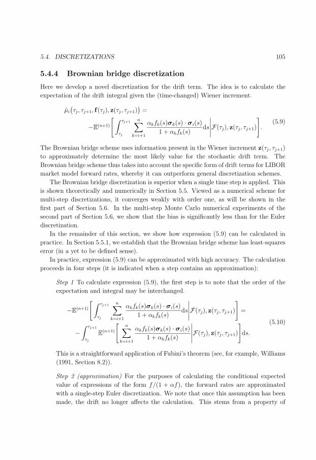
133

5.4. DISCRETIZATIONS 105

5.4.4 Brownian bridge discretization

Here we develop a novel discretization for the drift term. The idea is to calculate the

expectation of the drift integral given the (time-changed) Wiener increment.

µi


)=

−E(n+1)

[∫ τj+1

τj

n∑

k=i+1

αkfk(s)σk(s) · σi(s)

1 + αkfk(s)ds

∣∣∣∣∣F(τj), z(τj, τj+1)

].

(5.9)

The Brownian bridge scheme uses information present in the Wiener increment z(τj, τj+1)

to approximately determine the most likely value for the stochastic drift term. The

Brownian bridge scheme thus takes into account the specific form of drift terms for LIBOR

market model forward rates, whereby it can outperform general discretization schemes.

The Brownian bridge discretization is superior when a single time step is applied. This

is shown theoretically and numerically in Section 5.5. Viewed as a numerical scheme for

multi-step discretizations, it converges weakly with order one, as will be shown in the

first part of Section 5.6. In the multi-step Monte Carlo numerical experiments of the

second part of Section 5.6, we show that the bias is significantly less than for the Euler

discretization.

In the remainder of this section, we show how expression (5.9) can be calculated in

practice. In Section 5.5.1, we establish that the Brownian bridge scheme has least-squares

error (in a yet to be defined sense).

In practice, expression (5.9) can be approximated with high accuracy. The calculation

proceeds in four steps (it is indicated when a step contains an approximation):

Step 1 To calculate expression (5.9), the first step is to note that the order of the

expectation and integral may be interchanged.

−E(n+1)

[ ∫ τj+1

τj

n∑

k=i+1


1 + αkfk(s)ds

∣∣∣∣∣F(τj), z(τj, τj+1)

]=

−∫ τj+1

τj

E(n+1)

[n∑

k=i+1


1 + αkfk(s)

∣∣∣∣∣F(τj), z(τj, τj+1)

]ds.

(5.10)

This is a straightforward application of Fubini’s theorem (see, for example, Williams

(1991, Section 8.2)).

Step 2 (approximation) For the purposes of calculating the conditional expected

value of expressions of the form f/(1 + αf), the forward rates are approximated

with a single-step Euler discretization. We note that once this assumption has been

made, the drift no longer affects the calculation. This stems from a property of

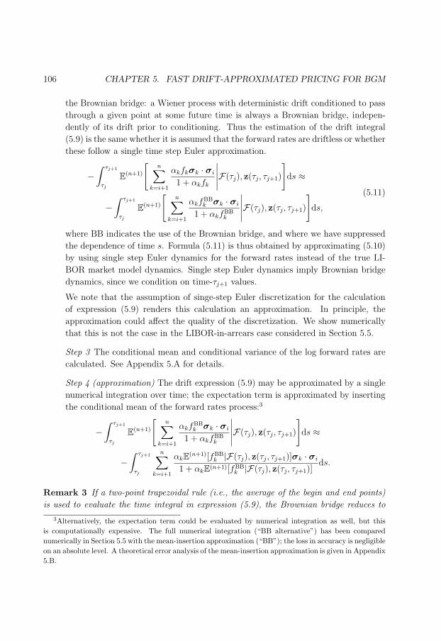
134


the Brownian bridge: a Wiener process with deterministic drift conditioned to pass

through a given point at some future time is always a Brownian bridge, indepen-

dently of its drift prior to conditioning. Thus the estimation of the drift integral

(5.9) is the same whether it is assumed that the forward rates are driftless or whether

these follow a single time step Euler approximation.

−∫ τj+1

τj

E(n+1)

[n∑

k=i+1

αkfkσk · σi

1 + αkfk

∣∣∣∣∣F(τj), z(τj, τj+1)

]ds ≈

−∫ τj+1

τj

E(n+1)

[n∑

k=i+1

αkfBBk σk · σi

1 + αkfBBk

∣∣∣∣∣F(τj), z(τj, τj+1)

]ds,

(5.11)

where BB indicates the use of the Brownian bridge, and where we have suppressed

the dependence of time s. Formula (5.11) is thus obtained by approximating (5.10)

by using single step Euler dynamics for the forward rates instead of the true LI-

BOR market model dynamics. Single step Euler dynamics imply Brownian bridge

dynamics, since we condition on time-τj+1 values.

We note that the assumption of singe-step Euler discretization for the calculation

of expression (5.9) renders this calculation an approximation. In principle, the

approximation could affect the quality of the discretization. We show numerically

that this is not the case in the LIBOR-in-arrears case considered in Section 5.5.

Step 3 The conditional mean and conditional variance of the log forward rates are

calculated. See Appendix 5.A for details.

Step 4 (approximation) The drift expression (5.9) may be approximated by a single

numerical integration over time; the expectation term is approximated by inserting

the conditional mean of the forward rates process:3

−∫ τj+1

τj

E(n+1)

[n∑

k=i+1

αkfBBk σk · σi

1 + αkfBBk

∣∣∣∣∣F(τj), z(τj, τj+1)

]ds ≈

−∫ τj+1

τj

n∑

k=i+1

αkE(n+1)[fBBk |F(τj), z(τj, τj+1)]σk · σi

1 + αkE(n+1)[fBBk |F(τj), z(τj, τj+1)]

ds.

Remark 3 If a two-point trapezoidal rule (i.e., the average of the begin and end points)

is used to evaluate the time integral in expression (5.9), the Brownian bridge reduces to

3Alternatively, the expectation term could be evaluated by numerical integration as well, but thisis computationally expensive. The full numerical integration (“BB alternative”) has been comparednumerically in Section 5.5 with the mean-insertion approximation (“BB”); the loss in accuracy is negligibleon an absolute level. A theoretical error analysis of the mean-insertion approximation is given in Appendix5.B.

135

5.5. THE BROWNIAN BRIDGE SCHEME FOR SINGLE TIME STEPS 107

the predictor-corrector scheme. In this sense, the predictor-corrector scheme is a special

case of the Brownian bridge scheme.

For illustration, MATLAB code is given in Appendix 5.C, implementing the Brownian

bridge scheme. The code implements a single time-step in a single-factor model with

constant volatility. These simplifications are for clarity of exposition only and are, of

course, not a restriction imposed by the Brownian bridge scheme.

We end this section with a discussion of the method used in this chapter for pric-

ing American-style options with Monte Carlo. The method used is the regression-based

method of Longstaff & Schwartz (2001), which is a method of stochastic mesh type (see

Broadie & Glasserman (2004)). Convergence of the method to the correct price follows

generically from the asymptotic convergence property of stochastic mesh methods, as

shown by Avramidis & Matzinger (2004).

5.5 The Brownian bridge scheme for single time steps

In this section, we establish theoretically and numerically that the Brownian bridge scheme

has superior accuracy for single time steps.

5.5.1 Theoretical result

Consider a stochastic differential equation of the form

dx(t) = µ(t,x(t)

)dt + Σ(t)dw(t). (5.12)

We note that the BGM log SDE (5.3) is of the above form. We consider a certain class

of discretizations:

Definition 4 Let the function µ(·, ·, ·) denote a single time step discretization of SDE

(5.12) with the following form:

y(τj+1) = y(τj) + µ(τj,y(τj), z(τj, τj+1)

)+ z(τj, τj+1). (5.13)

Here z(τj, τj+1) =∫ τj+1

τjσ(s)dw(s). Any such discretization is said to use information

about the Gaussian increment to estimate the drift term.

We note that Euler, predictor-corrector and Brownian bridge are such schemes. The next

theorem states that, for the BGM setting, the Brownian bridge scheme (5.9) has least-

squares error for a single time step over all discretizations that use information about the

Gaussian increment for the drift term.

136


Lemma 2 Let y be a single time step discretization of SDE (5.12) that uses informa-

tion about the Gaussian increment for the drift term. Consider the discretization expected

squared error

s2(y) := E

[∥∥y(τj+1)− xτj ,y(τj)(τj+1)∥∥2

∣∣∣F(τj)].

Here xt,y denotes the solution of SDE (5.12) starting from (t,y). Then the discretization

y∗ that yields least squared error, s2, over all possible discretizations that use informa-

tion about the Gaussian increment to estimate the drift term is defined by

µ∗(τj,y(τj), z(τj, τj+1))

= E[ ∫ τj+1

τj

µ(s,xτj ,y(τj)(s)

)ds

∣∣∣∣F(τj), z(τj, τj+1)

]. (5.14)

PROOF: Define

i :=

∫ τj+1

τj

µ(s,xτj ,y(τj)(s)

)ds.

For ease of exposition we write z = z(τj, τj+1) and µ = µ(τj,y(τj), z), but we keep in

mind that µ is F(τj), z-measurable. Also write Et[·] := E[·|F(t)]. Then let y′ with

drift term µ′ be a discretization of the form of Definition 4. First, we condition on z:

Eτj

[‖µ′ − i‖2∣∣z] ≥ Eτj

[‖Eτj[i|z]− i‖2

∣∣z] = Eτj

[‖µ∗ − i‖2∣∣z].

The inequality holds since expectation equals projection, and the latter has, by definition,

least squared error over all possible F(τj), z-measurable drift terms. Continuing, we

find

s2(y′) = Eτj

[‖µ′ − i‖2]

= Eτj

[Eτj

[‖µ′ − i‖2∣∣z]

]≥ Eτj

[Eτj

[‖µ∗ − i‖2∣∣z]

]= s2

(y∗),

i.e., y∗ has less squared error than y′. As y′ was an arbitrary discretization of the form

of Definition 4, the result follows. 2

5.5.2 LIBOR-in-arrears case

We estimate numerically the accuracy in the LIBOR-in-arrears test of the various schemes

of Section 5.4. We extend here the LIBOR-in-arrears test of Hunter et al. (2001) by

including the Milstein and Brownian bridge schemes. The test is designed to measure the

accuracy of a single time step discretization. The idea of the test is briefly described here;

for details the reader is referred to Hunter et al. (2001).

We consider the distribution of a forward rate under the measure associated with

the numeraire of a discount bond maturing at the fixing time of the forward. We note

that the forward rate is not a martingale under such a measure as the natural payment

time of the forward is not the same as its fixing time. An analytical formula for the

associated density, however, is known. We can thus compare the density obtained from

137

5.5. THE BROWNIAN BRIDGE SCHEME FOR SINGLE TIME STEPS 109

0

5

10

15

20

0.01% 0.10% 1.00% 10.00% 100.00%

f

den

sity analytical

Euler

predict-corr

Milstein

BB

BBalternativeSeries8

19

20

21

0.30% 0.40% 0.50% 0.60%

f

-0.1

0

0.1

0.2

0.3

0.4

0.5

0.6

0.01% 0.10% 1.00% 10.00% 100.00%

f

erro

r in

den

sity

analytical minusEuler

analytical minuspredictor corrector

analytical minusMilstein

analytical minusBrownian bridge

analytical minusBrownian bridgealternativeanalytical minus

Figure 5.1: Plots of the estimated densities and absolute errors in densities of various

single time step discretizations. The deal set-up is the same as in Hunter et al. (2001);

the three-month forward rate fixing 30 years from today is set initially to 8% and its

volatility to 24%. The legend key “BB” denotes Brownian bridge and “BB alternative”

denotes full numerical integration of the expectation term. We note that three densities

have been added to the above figures compared with Figure 1 of Hunter et al. (2001):

Milstein and the two Brownian bridge schemes. On both figures, however, the differences

between the analytical and Brownian bridge densities are indiscernible to the eye. The

most notable addition is the Milstein density. Outside of the error graph, the Milstein

scheme reaches a maximum absolute error that is around twice the maximum absolute

error for the Euler scheme. The maximum absolute error in the density for the Brownian

bridge and its alternative are 10−3 and 6 × 10−4, respectively. In this particular test

the Brownian bridge scheme thus achieves a reduction by a factor 100 in the maximum

absolute error over the predictor-corrector scheme, the latter being the second best scheme.

a single time step discretization with the analytical formula for the density. The results

of this test are displayed in Figure 5.1. It is shown (for the particular set-up) that the

Brownian bridge scheme reduces the maximum error in the density by a factor 100 over

the predictor-corrector scheme.

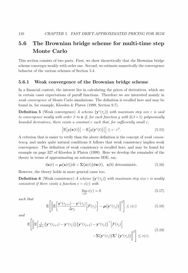
138


5.6 The Brownian bridge scheme for multi-time step

Monte Carlo

This section consists of two parts. First, we show theoretically that the Brownian bridge

scheme converges weakly with order one. Second, we estimate numerically the convergence

behavior of the various schemes of Section 5.4.

5.6.1 Weak convergence of the Brownian bridge scheme

In a financial context, the interest lies in calculating the prices of derivatives, which are

in certain cases expectations of payoff functions. Therefore we are interested mainly in

weak convergence of Monte Carlo simulations. The definition is recalled here and may be

found in, for example, Kloeden & Platen (1999, Section 9.7).

Definition 5 (Weak convergence) A scheme yε(τj) with maximum step size ε is said

to convergence weakly with order β to x if, for each function g with 2(β +1) polynomially

bounded derivatives, there exists a constant c such that, for sufficiently small ε,∣∣∣E[g(x(t)

)]− E[g(yε(t)

)]∣∣∣ ≤ c · εβ. (5.15)

A criterion that is easier to verify than the above definition is the concept of weak consis-

tency, and under quite natural conditions it follows that weak consistency implies weak

convergence. The definition of weak consistency is recalled here, and may be found for

example on page 327 of Kloeden & Platen (1999). Here we develop the remainder of the

theory in terms of approximating an autonomous SDE, say,

dx(t) = µ(x(t)

)dt + Σ

(x(t)

)dw(t), x(0) deterministic. (5.16)

However, the theory holds in more general cases too.

Definition 6 (Weak consistency) A scheme yε(τj) with maximum step size ε is weakly

consistent if there exists a function c = c(ε) with

limε↓0

c(ε) = 0 (5.17)

such that

E

[∥∥∥∥E[yε(τj+1)− yε(τj)

∆τj

∣∣∣∣F(τj)

]− µ

(yε(τj)

)∥∥∥∥2]≤ c(ε) (5.18)

and

E

[∥∥∥∥E[

1∆τj

yε(τj+1)− yε(τj)

yε(τj+1)− yε(τj)

>∣∣∣F(τj)]

−Σ(yε(τj)

)Σ>(

yε(τj))∥∥∥∥

2]≤ c(ε).

(5.19)

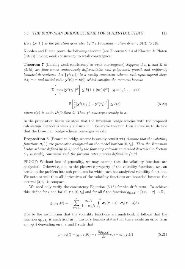
139

5.6. THE BROWNIAN BRIDGE SCHEME FOR MULTI-TIME STEPS 111

Here F(t) is the filtration generated by the Brownian motion driving SDE (5.16).

Kloeden and Platen prove the following theorem (see Theorem 9.7.4 of Kloeden & Platen

(1999)) linking weak consistency to weak convergence.

Theorem 7 (Linking weak consistency to weak convergence) Suppose that µ and Σ in

(5.16) are four times continuously differentiable with polynomial growth and uniformly

bounded derivatives. Let yε(τj) be a weakly consistent scheme with equitemporal steps

∆τj = ε and initial value yε(0) = x(0) which satisfies the moment bounds

E[

maxj|yε(τj)|2q

]≤ k

(1 + |x(0)|2q

), q = 1, 2, . . . and

E[1

ε

∣∣yε(τj+1)− yε(τj)∣∣6

]≤ c(ε), (5.20)

where c(ε) is as in Definition 6. Then yε converges weakly to x.

In the proposition below we show that the Brownian bridge scheme with the proposed

calculation method is weakly consistent. The above theorem then allows us to deduce

that the Brownian bridge scheme converges weakly.

Proposition 5 (Brownian bridge scheme is weakly consistent) Assume that the volatility

functions σi(·) are piece-wise analytical on the model horizon [0, tn]. Then the Brownian

bridge scheme defined by (5.9) and by the four-step calculation method described in Section

5.4 is weakly consistent with the forward rates process defined in (5.3).

PROOF: Without loss of generality, we may assume that the volatility functions are

analytical. Otherwise, due to the piecewise property of the volatility functions, we can

break up the problem into sub-problems for which each has analytical volatility functions.

We note as well that all derivatives of the volatility functions are bounded because the

interval [0, tn] is compact.

We need only verify the consistency Equation (5.18) for the drift term. To achieve

this, define for i and for all τ ∈ [0, tn] and for all f the function gi,τ,f : [0, tn − τ ] → R,

gi,τ,f(t) = −n∑

k=i+1

αkfk

1 + αkfk

∫ t

0

σk(τ + s) · σi(τ + s)ds.

Due to the assumption that the volatility functions are analytical, it follows that the

function gi,τ,f is analytical in t. Taylor’s formula states that there exists an error term

ei,τ,f(·) depending on i, τ and f such that

gi,τ,f(t) = gi,τ,f(0) + t∂gi,τ,f

∂t(0) + ei,τ,f(t) (5.21)

140


with

limt↓0

∣∣ei,τ,f(t)∣∣

t2< ∞. (5.22)

Due to the analyticity, bounded-ness and limiting behaviour of the function h(x) = x/(1+

x), namely h ↑ 1 (h ↓ 0) as x →∞ (x → −∞, respectively), we have that all its derivatives

are bounded. Viewed as a function [0, tn]× [0, tn]× Rn → R,

(t, τ, f) 7→ gi,τ,f(t),

we can thus find a bound on the second derivative ∂2gi,τ,f/∂t2, independent of (τ, f).

Theorem 7.7 of Apostol (1967) then states that the error term in (5.21) may be chosen

independently of τ and f . Hence we find that

gi,τ,f(t) = t

−

n∑

k=i+1

σk(τ) · σi(τ)αkfk

1 + αkfk

+ e(t),

with e satisfying the second-order Equation (5.22). Here we have used

gi,τ,f(0) = 0 and

∂gi,τ,f∂t

∣∣∣∣t=0

=

−

n∑

k=i+1

σk(τ) · σi(τ)αkfk

1 + αkfk

.

If Yε denotes the Brownian bridge scheme, then

E[yε

i (τj+1)− yεi (τj)

∣∣F(τj)]

= gi,τj ,Yε(τj)(ε)

= ε

−

n∑

k=i+1

αkyεk(τj)σk(τj) · σi(τj)

1 + αkyεk(τj)

+ e(ε).

We note that the term within braces is exactly drift term i evaluated at (τj,Yε(τj)). It

follows that consistency Equation (5.18) holds with c(ε) equal to (e(ε)/ε)2. The function

c(·) is then quadratic in ε. 2

Corollary 1 (Brownian bridge scheme converges weakly with order one) Under the as-

sumptions of Proposition 5, the Brownian bridge scheme defined by (5.9) and by the four-

step calculation method described in Section 5.4 converges weakly to the forward rates

process defined in (5.3). It has order of convergence one.

PROOF: We only need verify the claim with regards to the order of convergence. In the

proof of Theorem 7 in Kloeden & Platen (1999), it is shown that the error term in the

weak convergence criterion (5.15) is less than√

c(ε), with c(·) satisfying the requirements

(5.17), (5.18), (5.19) and (5.20). All these requirements can be met for the Brownian

bridge scheme with a quadratic function c. Taking the square root then yields first-order

weak convergence for the Brownian bridge scheme. 2

141

5.6. THE BROWNIAN BRIDGE SCHEME FOR MULTI-TIME STEPS 113

5.6.2 Numerical results

We now turn to the second part of Section 5.6, in which the various discretization schemes

are compared numerically. A floating leg and a cap were valued with 10 million simulation

paths. This large number of paths was used because the time discretization bias for the

log rates is small compared to the standard error often observed with 10,000 paths. For

example, the Euler one-step-per-accrual discretization relative bias for the floating leg and

the cap was estimated at 0.02% and 0.003%, whereas twice the standard error at 10,000

paths is 0.07% and 0.01%, respectively.

To obtain a bias-estimate with minimal standard error, we jointly simulate the values

of individual payments in the floating leg and cap under their respective forward mea-

sures. Such procedure filters out the discretization bias from the random noise in the

simulation. We note that, under the forward measure, there is no drift term and therefore

the associated payoff is an unbiased estimator of the value of the contract. If we denote

by πterminal and πfwd the numeraire-deflated contract payoff in the terminal and forward

measure, respectively, then an unbiased estimator of the bias is πterminal − πfwd. Alterna-

tively, we can benchmark against the analytical value πanalytical of the floating leg or cap,

which yields the unbiased estimator of the bias πterminal − πanalytical. The variances of the

two estimators are

Var[πterminal − πfwd

]= Var

[πterminal

]+ Var

[πfwd

]− 2Cov[πterminal, πfwd

](5.23)

Var[πterminal − πanalytical

]= Var

[πterminal

](5.24)

If we assume Var[πterminal

] ≈ Var[πfwd

], then (5.23) becomes

Var[πterminal − πfwd

] ≈ 2(1− ρ

[πterminal, πfwd

])Var

[πterminal

](5.25)

Therefore, if the correlation term ρ[πterminal, πfwd] is larger than 12, we have variance reduc-

tion. In our numerical LIBOR tests we found ρ ≈ 0.999, which means that the variance

is reduced by a factor of 500. The benchmark against the forward measure payoff is thus

also a useful tool when validating an implementation of a LIBOR market model, since a

bias that stems from an implementation error is more easily filtered out from the random

noise of the MC simulation.

The results are presented in Figure 5.2. They show that the predictor-corrector, Mil-

stein and Brownian bridge schemes have a time discretization bias that is hardly distin-

guishable from the standard error of the estimate. The Euler scheme, however, has a clear

time discretization bias for larger time steps. We classify the schemes from best suited to

worst suited (for the particular numerical cases under consideration) using the criterion

of the minimal computational time required to achieve a bias that is indistinguishable

142


Cap

-1E-07

0E+00

1E-07

2E-07

3E-07

4E-07

5E-07

6E-07

0 0.05 0.1 0.15 0.2 0.25 0.3

Time step (years)

Es

tim

ate

d b

ias

Euler

Predictor-corrector

Milstein

BB

Floating leg

-1E-05

0E+00

1E-05

2E-05

3E-05

4E-05

5E-05

6E-05

7E-05

0 0.2 0.4 0.6 0.8 1 1.2

Time step (years)

Es

tim

ate

d b

ias

Euler

Predictor-corrector

Milstein

BB

Figure 5.2: Plots of the estimated biases for a floating leg and a cap for the Euler,

predictor-corrector, Milstein and Brownian bridge schemes. A single-factor model was

applied. The floating leg is a six-year deal, with the fixings at 1, . . . , 5 years, and pay-

ments of annual LIBOR at 2, . . . , 6 years. The cap is a 1.5-year deal, with the fixings

at 0.25, 0.5, . . . , 1.25 years, and payments of quarterly LIBOR above 5% (if at all) at

0.5, 0.75, . . . , 1.5 years. The market conditions are the same for both deals: all initial

forward rates are 6%, and all volatility is constant at 20%. The net present values of the

floating leg and cap are 0.24 and 0.013, respectively, on a notional of one unit of currency.

The error bars denote a 95% confidence bound based on twice the sample standard error.

from the standard error at 10,000,000 paths. As Milstein is slightly faster than predictor-

corrector, which in turn is faster than the Brownian bridge, we obtain: first, Milstein;

second, predictor-corrector; third, Brownian bridge; and fourth, Euler. We stress here

that this classification might be particular to the numerical cases that we considered. We

also stress that the strength of the Brownian bridge lies in single time steps rather than

in multi-time steps.

5.7 An example: one-factor BGM framework with

drift approximations

This section illustrates the framework for fast single time step pricing in BGM by setting

it up in the special case of a one-factor model with a volatility structure as in Example

143

5.7. EXAMPLE: ONE-FACTOR DRIFT-APPROXIMATED BGM 115

1. This structure may be written as follows:

σi(t) = γieκt,

for certain constants γi. The corresponding Markov factor, x, is then defined as and

characterized by

x(t) =

∫ t

0

eκsdw(s), x(t) ∼ N (0, v(t)

), where

v(t) =

∫ t

0

e2κsds =

e2κt−1

2κ, κ 6= 0,

t, κ = 0.

Prices may now be computed by either numerical integration or finite differences. In

the case of numerical integration, if π(t, x) denotes the numeraire-deflated value of the

contingent claim, we have

π(0, x(0)

)=

∫ ∞

−∞π(t, x)p

(x; 0, v(t)

)dx

where t denotes the expiry of the contingent claim and p(·; µ, v) denotes the Gaussian

density with mean µ and standard deviation√

v. In case of finite differences, Feynman-

Kac yields the following PDE for the price relative to the terminal bond:

∂π

∂t+

1

2e2κt ∂

2π

∂x2= 0, (5.26)

with use of appropriate boundary conditions. For example, for a Bermudan payer swaption

we have π(·,−∞) ≡ 0, zero convexity ∂2π/∂x2 ≡ 0 at x = ∞, and exercise boundary

conditions at the exercise times.

5.7.1 A simple numerical example

We will evolve five annual (αi = 1) forward rates over a one-year period. Forward rate

i accrues from year i until year i + 1, i = 1, . . . , 5. Take fi(0) = 7%, γi = 25% and

κ = 15%; then v(1) ≈ 1.166196. Suppose that, after one year, the process x jumps to 1;

thus x(1) = 1. All computations are displayed in Table 5.1. Column (II) is determined

by (5.2). To evaluate the effect of the Brownian bridge scheme over the Euler scheme,

the “drift-frozen” forward rates (where the drift is evaluated at time zero) are displayed

in column (V), using the equation (V) = (I) exp ((II) + (III) + (IV)). Then, we start

with computing the Brownian bridge scheme forward rate 5 and work back to forward

rate 1. Forward rate 5 is easily computed as no drift terms are involved. To compute

the drift term integral at time 1 for forward rate 4, we compute the drift term integral of

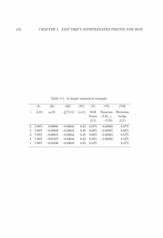
144


Table 5.1: A simple numerical example.

(I) (II) (III) (IV) (V) (VI) (VII)

i fi(0) µi(0) −12 γ2

i v(1) γix(1) Drift Equation Brownianfrozen (5.9)i−1 bridgefi(1) −(5.9)i fi(1)

5 7.00% 0.00000 −0.03644 0.25 8.67% −0.00569 8.67%4 7.00% −0.00409 −0.03644 0.25 8.63% −0.00567 8.62%3 7.00% −0.00818 −0.03644 0.25 8.60% −0.00564 8.57%2 7.00% −0.01227 −0.03644 0.25 8.56% −0.00562 8.53%1 7.00% −0.01636 −0.03644 0.25 8.53% 8.47%

145

5.8. EXAMPLE: BERMUDAN SWAPTION 117

(5.9) for forward rate 5. The result is displayed in column (VI). This we may then use

to compute the Brownian bridge scheme forward rate 4 (see column (VII)), where we use

the equation (VII)i = (I)exp(∑nj=i+1(VI)j + (III) + (IV)). Continuing, we compute the

drift for forward rate 3 using only the Brownian bridge forward rates 4 and 5. And so on

until all forward rates have been computed.

5.8 Example: Bermudan swaption

As an example of the single time step pricing framework, an analysis is made for Bermudan

swaptions in comparison with a BGM model combined with the least-squares Monte Carlo

method introduced by Longstaff & Schwartz (2001). The one-factor set-up introduced in

the previous section was used with zero mean-reversion.

Callable Bermudan and European payer swaptions were priced in a one-factor BGM

model for various tenors and non-call periods. The zero rates were taken to be flat at 5%,

and the volatility of the forwards was set flat at 15%. The Bermudans were priced on a

grid, the Europeans through numerical integration. The PDE was solved using an explicit

finite-difference scheme. The explanatory variable in the least-squares Monte Carlo was

taken to be the net present value (NPV) of the underlying swap. This was regressed on to

a constant and a linear term. These two basis functions yield sufficiently accurate results

because the value of a Bermudan swaption increases almost linearly with the value of the

underlying swap.

Problems may possibly occur for American-style derivatives in the single time step

framework. Since the framework is not arbitrage-free, spurious early or delayed exercise

may take place to collect the arbitrage opportunity. The effects of these phenomena have

been analyzed by comparing the exercise boundaries4 and risk sensitivities of Longstaff-

Schwartz and single time step BGM. In both models the exercise rule turned out to be of

the following form: exercise whenever the NPV of the underlying swap, s, is larger than

a certain value s∗, which is then defined to be the exercise boundary.

For a full description of the deal see Table 5.2. Results have been summarized in Table

5.3. Computational times may be found in Table 5.4. Exercise boundaries for the 8 year

deal are displayed in Figure 5.3, including confidence bounds on the Longstaff-Schwartz

4In the Longstaff-Schwartz case, the future discounted cashflows are regressed against the NPV ofthe underlying swap with a constant and linear term – say, with coefficients a and b. So the option isexercised whenever s > a + bs ⇔ s > a/(1 − b) =: s∗, where it is assumed that b < 1, which turns outto hold in practice. Hence the exercise boundary s∗ may be computed from the regression coefficients bythe above formula.

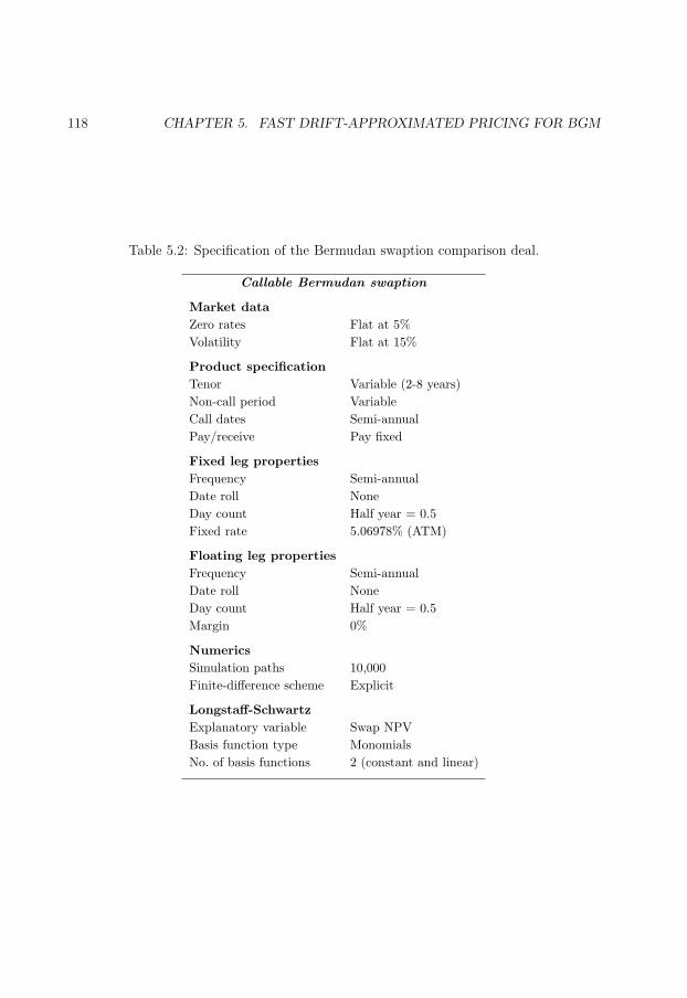
146


Table 5.2: Specification of the Bermudan swaption comparison deal.

Callable Bermudan swaption

Market dataZero rates Flat at 5%Volatility Flat at 15%

Product specificationTenor Variable (2-8 years)Non-call period VariableCall dates Semi-annualPay/receive Pay fixed

Fixed leg propertiesFrequency Semi-annualDate roll NoneDay count Half year = 0.5Fixed rate 5.06978% (ATM)

Floating leg propertiesFrequency Semi-annualDate roll NoneDay count Half year = 0.5Margin 0%

NumericsSimulation paths 10,000Finite-difference scheme Explicit

Longstaff-SchwartzExplanatory variable Swap NPVBasis function type MonomialsNo. of basis functions 2 (constant and linear)

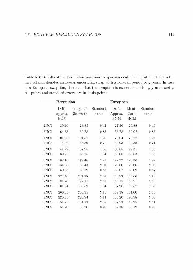
147


Table 5.3: Results of the Bermudan swaption comparison deal. The notation xNCy in the

first column denotes an x-year underlying swap with a non-call period of y years. In case

of a European swaption, it means that the swaption is exercisable after y years exactly.

All prices and standard errors are in basis points.

Bermudan European

Drift- Longstaff- Standard Drift- Monte Standardapprox. Schwartz error Approx. Carlo errorBGM BGM BGM

2NC1 29.40 28.85 0.42 27.36 26.88 0.43

3NC1 64.33 62.78 0.83 53.78 52.92 0.83

4NC1 101.66 101.51 1.29 78.04 78.77 1.244NC3 44.09 43.59 0.70 42.93 42.55 0.71

5NC1 141.22 137.95 1.68 100.85 99.31 1.555NC3 89.25 86.75 1.34 83.08 80.83 1.36

6NC1 182.16 179.48 2.22 122.27 123.36 1.926NC3 134.88 136.43 2.01 120.60 123.06 2.036NC5 50.93 50.79 0.86 50.07 50.09 0.87

7NC1 224.40 221.38 2.61 142.93 140.66 2.197NC3 181.20 177.11 2.53 156.15 153.71 2.537NC5 101.84 100.59 1.64 97.28 96.57 1.65

8NC1 266.63 266.35 3.15 159.38 161.00 2.508NC3 226.55 226.94 3.14 185.20 190.98 3.088NC5 151.23 151.13 2.38 137.73 140.95 2.418NC7 54.20 53.70 0.96 52.38 53.12 0.96

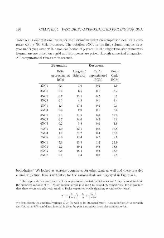
148


Table 5.4: Computational times for the Bermudan swaption comparison deal for a com-

puter with a 700 MHz processor. The notation xNCy in the first column denotes an x-

year underlying swap with a non-call period of y years. In the single time step framework

Bermudans are priced on a grid and Europeans are priced through numerical integration.

All computational times are in seconds.

Bermudan European

Drift- Longstaff Drift- Monteapproximated Schwartz approximated Carlo

BGM BGM BGM

2NC1 0.4 3.0 0.0 1.9

3NC1 0.4 6.6 0.1 3.7

4NC1 0.7 11.1 0.2 6.14NC3 0.2 4.5 0.1 3.4

5NC1 1.4 17.3 0.6 9.15NC3 0.3 9.0 0.1 6.2

6NC1 2.4 24.5 0.6 12.86NC3 0.7 14.6 0.2 9.86NC5 0.2 5.8 0.0 4.8

7NC1 4.0 33.1 0.8 16.87NC3 1.4 21.2 0.4 13.57NC5 0.3 11.4 0.2 8.6

8NC1 5.6 45.9 1.2 23.98NC3 2.2 30.2 0.6 18.88NC5 0.6 18.4 0.2 13.58NC7 0.1 7.4 0.0 7.8

boundaries.5 We looked at exercise boundaries for other deals as well and these revealed

a similar picture. Risk sensitivities for the various deals are displayed in Figure 5.4.

5The empirical covariance matrix of the regression-estimated coefficients a and b may be used to obtainthe empirical variance of s∗. Denote random errors in a and b by εa and εb, respectively. If it is assumedthat these errors are relatively small, a Taylor expansion yields (ignoring second-order terms)

s∗ ≈ a

1− b

(1 +

εa

a+

εb

1− b

).

We thus obtain the empirical variance of s∗ (as well as its standard error). Assuming that s∗ is normallydistributed, a 95% confidence interval is given by plus and minus twice the standard error.

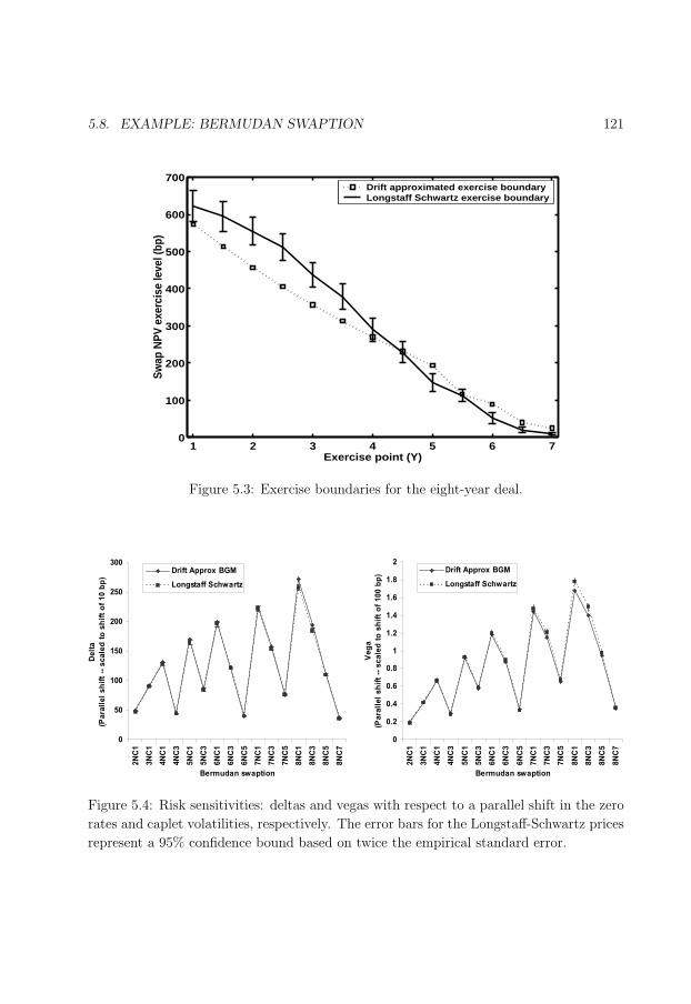
149


1 2 3 4 5 6 70

100

200

300

400

500

600

700

Exercise point (Y)

Swap

NPV

exe

rcis

e le

vel (

bp)

Drift approximated exercise boundaryLongstaff Schwartz exercise boundary

Figure 5.3: Exercise boundaries for the eight-year deal.

0

50

100

150

200

250

300

2N

C1

3N

C1

4N

C1

4N

C3

5N

C1

5N

C3

6N

C1

6N

C3

6N

C5

7N

C1

7N

C3

7N

C5

8N

C1

8N

C3

8N

C5

8N

C7

Bermudan swaption

De

lta

(Pa

rall

el

sh

ift

-- s

ca

led

to

sh

ift

of

10

bp

)

Drift Approx BGM

Longstaff Schwartz

0

0.2

0.4

0.6

0.8

1

1.2

1.4

1.6

1.8

2

2N

C1

3N

C1

4N

C1

4N

C3

5N

C1

5N

C3

6N

C1

6N

C3

6N

C5

7N

C1

7N

C3

7N

C5

8N

C1

8N

C3

8N

C5

8N

C7

Bermudan swaption

Ve

ga

(Pa

rall

el

sh

ift

-- s

ca

led

to

sh

ift

of

10

0 b

p)

Drift Approx BGM

Longstaff Schwartz

Figure 5.4: Risk sensitivities: deltas and vegas with respect to a parallel shift in the zero

rates and caplet volatilities, respectively. The error bars for the Longstaff-Schwartz prices

represent a 95% confidence bound based on twice the empirical standard error.

150


Table 5.5: BGM pricing simulation re-run for 500,000 paths using pre-computed exercise

boundaries. The standard errors for both prices were virtually the same in all cases,

therefore only a single standard error is reported. All prices and standard errors are in

basis points.

BGM simulation price

LS pre-computed DA pre-computed Standard error

exercise boundaries exercise boundaries

2NC1 28.63 28.62 0.06

3NC1 62.80 62.77 0.12

4NC1 99.51 99.58 0.18

5NC1 138.38 138.55 0.24

6NC1 178.08 179.41 0.30

7NC1 221.51 222.49 0.36

8NC1 263.05 265.27 0.42

The results show that the single time step BGM pricing framework indeed prices the

Bermudan swaptions close to Longstaff-Schwartz, including correct estimates of risk sen-

sitivities for shorter-maturity deals. In all cases the price difference is within twice the

standard error of the simulation. Moreover, the computational time involved is less by

a factor 10. We note that the exercise boundary is calculated slightly differently by the

Longstaff-Schwartz and drift-approximated (DA) approach. Also, risk sensitivities for

longer-maturity deals (seven to eight years) can be outside of the two-standard-error con-

fidence bound. The Brownian bridge drift approximation thus becomes worse for longer-

maturity deals, as also explained in Section 5.9. To determine which approach computed

the best exercise boundaries, the BGM pricing simulation was re-run for 500,000 paths

using the pre-computed exercise boundaries. The results, given in Table 5.5, show that

the drift-approximated exercise boundaries are not worse than their Longstaff-Schwartz

counterparts and are even slightly better.6 Hence there is no problem with the spurious

early exercise opportunities arising from the absence of no-arbitrage in the fast single time

step framework. The non-arbitrage-free issue is investigated further in the next section.

This section ends with the results for a two-factor model.

6This does not necessarily mean that the DA framework outperforms Longstaff-Schwartz because weonly regress on the NPV of the underlying swap. Longstaff-Schwartz may possibly yield better exerciseboundaries when it is regressed on to more explanatory variables.

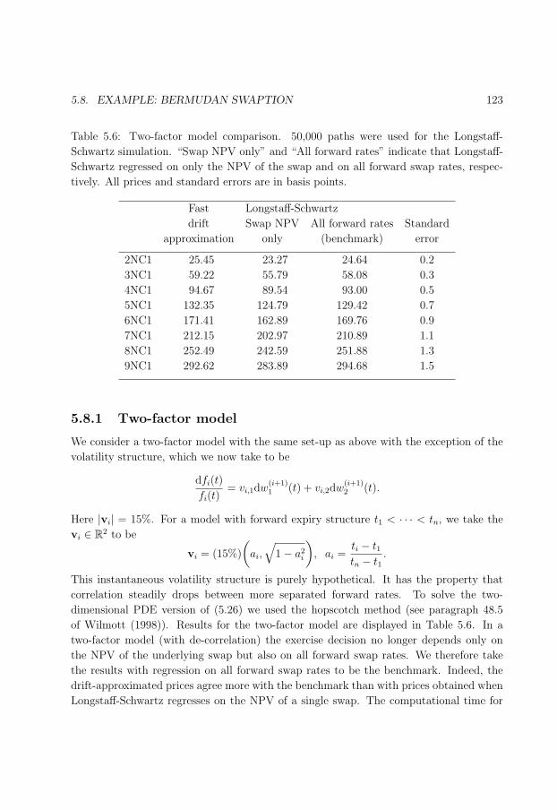
151


Table 5.6: Two-factor model comparison. 50,000 paths were used for the Longstaff-

Schwartz simulation. “Swap NPV only” and “All forward rates” indicate that Longstaff-

Schwartz regressed on only the NPV of the swap and on all forward swap rates, respec-

tively. All prices and standard errors are in basis points.

Fast Longstaff-Schwartz

drift Swap NPV All forward rates Standard

approximation only (benchmark) error

2NC1 25.45 23.27 24.64 0.2

3NC1 59.22 55.79 58.08 0.3

4NC1 94.67 89.54 93.00 0.5

5NC1 132.35 124.79 129.42 0.7

6NC1 171.41 162.89 169.76 0.9

7NC1 212.15 202.97 210.89 1.1

8NC1 252.49 242.59 251.88 1.3

9NC1 292.62 283.89 294.68 1.5

5.8.1 Two-factor model

We consider a two-factor model with the same set-up as above with the exception of the

volatility structure, which we now take to be

dfi(t)

fi(t)= vi,1dw

(i+1)1 (t) + vi,2dw

(i+1)2 (t).

Here |vi| = 15%. For a model with forward expiry structure t1 < · · · < tn, we take the

vi ∈ R2 to be

vi = (15%)

(ai,

√1− a2

i

), ai =

ti − t1tn − t1

.

This instantaneous volatility structure is purely hypothetical. It has the property that

correlation steadily drops between more separated forward rates. To solve the two-

dimensional PDE version of (5.26) we used the hopscotch method (see paragraph 48.5

of Wilmott (1998)). Results for the two-factor model are displayed in Table 5.6. In a

two-factor model (with de-correlation) the exercise decision no longer depends only on

the NPV of the underlying swap but also on all forward swap rates. We therefore take

the results with regression on all forward swap rates to be the benchmark. Indeed, the

drift-approximated prices agree more with the benchmark than with prices obtained when

Longstaff-Schwartz regresses on the NPV of a single swap. The computational time for

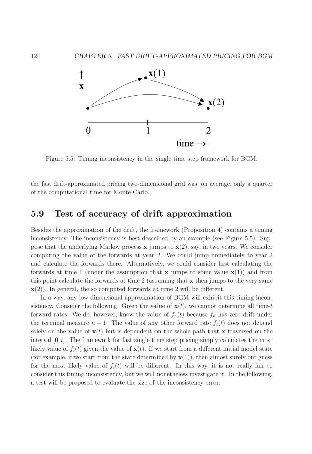
152


10 2

x

x(1)

x(2)

time

Figure 5.5: Timing inconsistency in the single time step framework for BGM.

the fast drift-approximated pricing two-dimensional grid was, on average, only a quarter

of the computational time for Monte Carlo.

5.9 Test of accuracy of drift approximation

Besides the approximation of the drift, the framework (Proposition 4) contains a timing

inconsistency. The inconsistency is best described by an example (see Figure 5.5). Sup-

pose that the underlying Markov process x jumps to x(2), say, in two years. We consider

computing the value of the forwards at year 2. We could jump immediately to year 2

and calculate the forwards there. Alternatively, we could consider first calculating the

forwards at time 1 (under the assumption that x jumps to some value x(1)) and from

this point calculate the forwards at time 2 (assuming that x then jumps to the very same

x(2)). In general, the so computed forwards at time 2 will be different.

In a way, any low-dimensional approximation of BGM will exhibit this timing incon-

sistency. Consider the following. Given the value of x(t), we cannot determine all time-t

forward rates. We do, however, know the value of fn(t) because fn has zero drift under

the terminal measure n + 1. The value of any other forward rate fi(t) does not depend

solely on the value of x(t) but is dependent on the whole path that x traversed on the

interval [0, t]. The framework for fast single time step pricing simply calculates the most

likely value of fi(t) given the value of x(t). If we start from a different initial model state

(for example, if we start from the state determined by x(1)), then almost surely our guess

for the most likely value of fi(t) will be different. In this way, it is not really fair to

consider this timing inconsistency, but we will nonetheless investigate it. In the following,

a test will be proposed to evaluate the size of the inconsistency error.

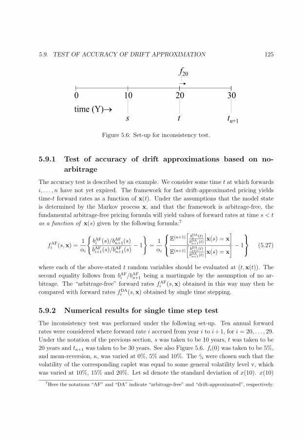
153

5.9. TEST OF ACCURACY OF DRIFT APPROXIMATION 125

20100

time (Y)

30

f20

s t tn+1

Figure 5.6: Set-up for inconsistency test.

5.9.1 Test of accuracy of drift approximations based on no-

arbitrage

The accuracy test is described by an example. We consider some time t at which forwards

i, . . . , n have not yet expired. The framework for fast drift-approximated pricing yields

time-t forward rates as a function of x(t). Under the assumptions that the model state

is determined by the Markov process x, and that the framework is arbitrage-free, the

fundamental arbitrage-free pricing formula will yield values of forward rates at time s < t

as a function of x(s) given by the following formula:7

fAFi (s,x) =

1

αi

bAFi (s)/bAF

n+1(s)

bAFi+1(s)/b

AFn+1(s)

− 1

=

1

αi

E(n+1)

[bDAi (t)

bDAn+1(t)

∣∣∣x(s) = x]

E(n+1)[

bDAi+1(t)

bDAn+1(t)

∣∣∣x(s) = x] − 1

(5.27)

where each of the above-stated t random variables should be evaluated at (t,x(t)). The

second equality follows from bAFi /bAF

n+1 being a martingale by the assumption of no ar-

bitrage. The “arbitrage-free” forward rates fAFi (s,x) obtained in this way may then be

compared with forward rates fDAi (s,x) obtained by single time stepping.

5.9.2 Numerical results for single time step test

The inconsistency test was performed under the following set-up. Ten annual forward

rates were considered where forward rate i accrued from year i to i+1, for i = 20, . . . , 29.

Under the notation of the previous section, s was taken to be 10 years, t was taken to be

20 years and tn+1 was taken to be 30 years. See also Figure 5.6. fi(0) was taken to be 5%,

and mean-reversion, κ, was varied at 0%, 5% and 10%. The γi were chosen such that the

volatility of the corresponding caplet was equal to some general volatility level v, which

was varied at 10%, 15% and 20%. Let sd denote the standard deviation of x(10). x(10)

7Here the notations “AF” and “DA” indicate “arbitrage-free” and “drift-approximated”, respectively.

154


Table 5.7: Quality of drift approximations: comparison of fAF20 (10) and fDA

20 (10) under

different x(10) moves for the volatility/mean-reversion scenario 15%/10%. sd denotes the

standard deviation of x(10). All variables are evaluated at time t=10.

Brownian Bridge

x(10) fAF20 fDA

20 fDA20 − fAF

20

(%) (%) (bp)

−sd 3.75 3.81 5.11

−sd/2 4.23 4.27 4.03

0 4.77 4.79 2.37

+sd/2 5.38 5.38 -0.05

+sd 6.07 6.03 -3.47

Predictor-corrector

x(10) fAF20 fDA

20 fDA20 − fAF

20

(%) (%) (bp)

−sd 3.74 3.81 7.17

−sd/2 4.19 4.27 7.94

0 4.70 4.79 8.81

+sd/2 5.28 5.38 9.79

+sd 5.92 6.03 10.91

Table 5.8: Quality of drift approximations: Maximum of |fAF20 (10)− fDA

20 (10)| over x(10)

moves 0,±sd/2,±sd for different volatility/mean-reversion scenarios. sd denotes the stan-

dard deviation of x(10). Differences are denoted in basis points.

Brownian Bridge

Mean- Volatility level (v)

reversion 10% 15% 20%

0% 2.97 9.34 28.73

5% 2.56 8.21 19.46

10% 1.46 5.11 12.56

Predictor-corrector

Mean- Volatility level (v)

reversion 10% 15% 20%

0% 2.86 8.60 37.45

5% 2.32 12.29 53.85

10% 1.69 10.91 44.59

moves were considered for 0,±sd/2, and ±sd. Results for the volatility/mean-reversion

scenario 15%/10% are given in Table 5.7. The comparison is only reported for f20 because

this forward rate contains the most drift terms, and therefore its corresponding error is

the largest among i = 20, . . . , 29. We note that the error for f29 is always zero as it is

fully determined by x. In Table 5.8 the maximum error (over the five considered x(10)

moves) between fAF20 (10) and fDA

20 (10) is reported.

The test was performed for both the Brownian bridge and predictor-corrector schemes.

The results show that the former outperforms the latter in the timing inconsistency test.

The inconsistency test results show that, for less volatile market scenarios, the single

time step framework performs very accurately, with errors only up to a few basis points.

155

5.10. CONCLUSIONS 127

For more volatile market scenarios the approximation deteriorates. But for realistic yield

curve and forward volatility scenarios there are no problems with respect to pricing (see

Section 5.8). The worsening of the approximation for more volatile scenarios is what

may be expected from the nature of the drift approximations: as the model dimensions

increase, the single time step approximation will break up. By “model dimensions” we

mean the volatility level, the tenor of the deal, the difference between the forward index

i and n, or time zero forward rates, etc. Care should be taken in applying the single time

step framework for BGM that the market scenario does not violate the realm where the

single time step approximation is reasonably valid.

5.10 Conclusions

We have introduced a fast approximate pricing framework as an addition to the predictor-

corrector drift approximation developed by Hunter et al. (2001). These authors used the

drift approximation only to speed up their Monte Carlo by reducing it to single time step

simulation. We have shown that, at a slight cost, much faster computational methods

may be used, such as numerical integration or finite differences. The additional cost is a

non-restrictive assumption, namely, separability of the volatility function. The proposed

drift approximation framework was applied to the pricing of Bermudan swaptions, for

which it yielded very accurate prices with much lower computation times.

5.A Appendix: Mean of geometric Brownian bridge

In this appendix, the time-t mean of the process fk defined in (5.9) is determined. Equiv-

alently, we may determine the time-t mean of the process y, given by

dy(t)

y(t)= σ(t) · dw(t), y(0) = y0, y(t∗) = y∗.

(Compare with (5.9).) The solution of y (unconditional of time-t∗) is given by

y(t) = y0ex(t)− 1

2v(t),

where

x(t) :=

∫ t

0

σ(s) · dw(s), v(t) :=

∫ t

0

‖σ(s)‖2ds.

We note that

ω ∈ Ω; y(t∗) = y∗

=

ω ∈ Ω; x(t∗) = log(y∗/y0) +

1

2v(t∗) =: x∗

.

156


According to the martingale time change theorem (for example Theorem 4.6 of Karatzas

& Shreve (1991)), we have that x(τ(·)) is a Brownian motion, where the time change τ is

defined by

τ(t) = infs ≥ 0; v(t) > s.Working in the time-changed time coordinates, x(·)|x(τ ∗) = x∗ is a standard Brownian

bridge, and so, according to Section 5.6.B of Karatzas & Shreve (1991),

(x(τ)

∣∣x(τ ∗) = x∗) ∼ N

(τ

τ ∗x∗, τ − τ 2

τ ∗

).

Back in the original time coordinates, this translates to

(x(t)

∣∣x(t∗) = x∗) ∼ N

(v(t)

v(t∗)x∗, v(t)−

(v(t)

)2

v(t∗)

).

With this, we may evaluate the mean of (y(t)|y(t∗) = y∗) to be

E[y(t)

∣∣y(t∗) = y∗]

= y0

(y∗

y0

) v(t)v(t∗)

exp

1

2

v(t)

v(t∗)

(v(t∗)− v(t)

), (5.28)

where the following simple rule has been used: E[ez] = eβ+τ2/2 whenever z is normally

distributed, z ∼ N (β, τ 2).

5.B Appendix: Approximation of substituting the

mean in the expectation of expression (5.9)

In Section 5.3 a four-step method for the calculation of expression (5.9) is described. An

approximating fourth step is proposed that evaluates the expectation of the BGM drift

inserting the mean. In this appendix an error bound for this approximation is derived,

and it is shown that the approximation is of order two in volatility in the neighbourhood

of zero.

The expectation term can always be rewritten as

g(µ, σ) = E[

expµ + σz1 + expµ + σz

],

where z is distributed standard normally. It is straightforward to verify that the above

function g : R2 → R is infinitely differentiable at every point of the whole real plane.

We note that approximating the above expectation at the mean signifies that the above

function is approximated as

g(µ, σ) ≈ g(µ, 0) =expµ

1 + expµ .

157

5.C. APPENDIX: MATLAB CODE FOR BROWNIAN BRIDGE SCHEME 129

Fix µ and calculate the derivative of g with respect to σ. The interchange of differentiation

and expectation is a subtle argument that may, for example, be found in Williams (1991,

paragraph A.16.1). We carefully verified that in the above case all the requirements for

interchange are satisfied. We then find

∂g

∂σ(µ, σ) = E

[z

expµ + σz(1 + expµ + σz)2

].

Due to the odd nature of the above integrand at the point σ = 0, we find that

∂g

∂σ(µ, 0) = 0.

Taylor’s formula then states that there exists c ≥ 0 (possibly depending on µ) such that

∣∣∣∣g(µ, σ)− expµ1 + expµ

∣∣∣∣ ≤ cσ2.

Because a bound on the second derivative of σ 7→ g(µ, σ) may be found independently of

µ on some interval [0, σ], it follows from Theorem 7.7 of Apostol (1967) that the constant

c may then be chosen independently of µ for all σ ∈ [0, σ].

5.C Appendix: MATLAB code for Brownian bridge

scheme

MATLAB code illustrating the Brownian bridge scheme and the four-steps calculation

method in Section 5.4, is displayed below.

function result = fBB(n,f0,a,vol,t,z)

% Calculates forward LIBOR rates in one-factor model with Brownian bridge

% drift approximation & single time step, given the normal increment z.

% n, no. of forward LIBORs, a positive integer

% f0, array with n elements, time zero forward LIBORs

% a, array with n elements, day count fractions

% vol, array with n elements, vol[i] = volatility of forward LIBOR i

% t, time (scalar)

% z, Gaussian increment ~N(0,1), scalar

% f is used to store result

f=zeros(n,1); % creates zero array with n entries

158


% First do ultimate forward LIBOR => martingale!

f(n)=f0(n)*exp(-0.5*vol(n)^2*t+vol(n)*sqrt(t)*z);

% Loop from penultimate LIBOR down to first LIBOR.

run_drift=0.0; % used for efficient calculation of drift

for i=n-1:-1:1

zt=log(f(i+1)/f0(i+1))+0.5*vol(i+1)^2*t; % Needed for driftBB.

% quad is a standard integration routine in MATLAB.

% quad(@f,a,b,tol,trace,p1,p2,...) integrates the function

% f(s,p1,p2,...) over s from a to b with convergence criteria tol and

% trace.

% For definitions of tol and trace we refer to MATLAB documentation.

% Of course, one can use any integration routine instead of quad.

% Adjusting the convergence criterion of the numerical integrator

% allows for a trade-off between accuracy and computational speed.

% For example, the predictor-corrector scheme is a special case of

% the Brownian bridge scheme if the crudest integrator (two-point

% trapezoid) is used.

run_drift=run_drift ...

-quad(@driftBB,0.0,t,1.0e-6,0,f0(i+1),a(i+1),vol(i+1),t,zt);

% Equation (5.3) in exp form

f(i)=f0(i)*exp((run_drift*vol(i)-0.5*vol(i)^2*t)+vol(i)*sqrt(t)*z);

end

result = f; % return result f

function result = driftBB(s,f0,a,vol,t,zt)

% Calculates drift term evaluated at the mean of the Brownian bridge.

% This function will be integrated over time.

% s, scalar, current (intermediate) time

% f0, scalar, time zero forward LIBOR

% a, scalar, day count fraction

% vol, scalar, volatility of forward LIBOR

% t, scalar, time (at which forward LIBOR has already been predicted)

% zt, scalar, help variable associated with LIBOR predicted at time t

% Mean of Brownian bridge, Equation (5.26) in log-form:

m=s./t.*zt-0.5.*vol.^2.*s.*s./t+log(f0)+log(a);

159

5.C. APPENDIX: MATLAB CODE FOR BROWNIAN BRIDGE SCHEME 131

% Essential form of BGM drift in terms of log rates:exp(.)/(1+exp(.)):

result=vol*exp(m)./(1.0+exp(m));

160


161

Chapter 6

A comparison of single factor

Markov-functional and multi factor

market models

We compare single factor Markov-functional and multi factor market models for hedging

performance of Bermudan swaptions. We show that hedging performance of both models

is comparable, thereby supporting the claim that Bermudan swaptions can be adequately

risk-managed with single factor models. Moreover, we show that the impact of smile can

be much larger than the impact of correlation. We propose a new method for calculating

risk sensitivities of callable products in market models, which is a modification of the

least-squares Monte Carlo method. The hedge results show that this new method enables

proper functioning of market models as risk-management tools.

6.1 Introduction

Bermudan swaptions form a popular class of interest rate derivatives. The underlying

is a plain-vanilla interest rate swap, in which periodic fixed payments are exchanged for

floating LIBOR payments. Institutional debt issuers use interest rate swaps to revert from

floating to fixed interest rate payments, and vice versa. Often the issuers want to reserve

the right to cancel the swap. A cancellable swap can be valued by the following parity

relation. A cancellable interest rate swap is equal to a plain-vanilla interest rate swap

plus a callable interest rate swap with reversed cash flows. Thus a cancellable swap can

be valued when the callable swap can be valued. Such callable swap options are referred

to as Bermudan swaptions. Bermudan means that the exercise opportunities are at a

discrete set of time points. A European swaption is an option to enter into a swap at only

a single exercise date.

162

134 CHAPTER 6. COMPARISON OF SINGLE AND MULTI FACTOR MODELS

In this chapter, we will study the pricing and hedging performance of two popular

models for Bermudan swaptions. Many models have been proposed in the literature for

valuation and risk management of Bermudan swaptions. We distinguish three categories:

short-rate models, Markov-functional models and market models.

Short-rate models model the dynamics of the term structure of interest rates by spec-

ifying the dynamics of a single rate (the short rate) from which the whole term structure

at any point in time can be calculated. Examples of short-rate models include the models

of Vasicek (1977), Cox et al. (1985), Dothan (1978), Black et al. (1990), Ho & Lee (1986)

and Hull & White (1990).

The Markov-functional model of Hunt et al. (2000) assumes that the discount factors

are a function of some underlying Markov process. The model is then fully determined by

no-arbitrage arguments and by requiring a fit to the initial yield curve and interest rate

option volatility.

Market models were introduced by Brace et al. (1997), Miltersen et al. (1997) and

Jamshidian (1997). The name ‘market model’ refers to the modelling of market observable

variables such as LIBOR rates and swap rates. The explicit modelling of market rates

allows for natural formulas for interest rate option volatility, that are consistent with the

market practice of using the formula of Black (1976) for caps (options on LIBOR) and

swaptions (options on swap rates).

Short-rate and Markov-functional models are usually1 implemented as models with

a single stochastic process driving the term structure of interest rates. A disadvantage

is then that the instantaneous correlation between interest rates can only be 1. Market

models however efficiently allow for any number of stochastic variables to be used, so that

any instantaneous correlation structure can be captured. There is substantial evidence

that the term structure of interest rates is driven by multiple factors (three, four, or even

more), see the review article of Dai & Singleton (2003). A more realistic description of

reality may thus be expected from multi factor models, which points to possibly better

hedge performance. The question addressed in this chapter is whether the increase in

hedge performance due to use of a multi factor model is significant. To those that a

priori dismiss the use of single factor models due to their economic irrelevance by failure

in capturing the multi factor dynamics of the term structure of interest rates, we say:

Models that are best for managing an interest rate derivatives book are not necessarily

models that are most realistic, rather they are models that most reduce variance of profit

and loss (P&L), thereby preserving wealth in the most stable manner. We mention four

articles that compare single and multi factor models.

First, in favour of multi factor models, Longstaff et al. (2001) claim that short-rate

models, because of supposedly misspecified dynamics, lead to suboptimal exercise strate-

1Two factor short rate models exist too, see for example Ritchken & Sankarasubramanian (1995).

163


gies. This claim is supported by empirical evidence performed with the short-rate models

of Black et al. (1990) and Black & Karasinski (1991). The authors then conclude that

the costs to Wall Street firms of following single factor exercise strategies could be several

billion dollars. The argument of Andersen & Andreasen (2001), and also ours, against

the claim of Longstaff et al. (2001), is that their choice of calibration does not correspond

to market practice and leads to models that are poorly fitted to market.

Second, in favour of single factor models, Andersen & Andreasen (2001) claim that

the exercise strategy obtained from a properly calibrated single factor model only leads

to insignificant losses when applied in a two factor model.

Third, Driessen, Klaassen & Melenberg (2003) are the first to investigate hedge perfor-

mance. These authors investigate two types of delta hedge instruments, (i) a number of

delta hedge securities, i.e. discount bonds, equal to the number of factors, and (ii) a large

set of discount bonds, one for each security spanning the yield curve. They show that

if the number of hedge instruments is equal to the number of factors, then multi factor

models outperform single factor models. If, however, the large set of hedging instruments

is used, which is the case in practice, then single factor models perform as well as multi

factor models in terms of delta hedging of European swaptions.

Fourth, Fan, Gupta & Ritchken (2003) show, for the case of the number of hedge

instruments equal to the number of factors, that higher factor models perform better

than lower factor models in terms of delta hedging of European swaptions and European

swaption straddles2. The results of Fan et al. (2003) are thus consistent with the findings

of Driessen et al. (2003).

Relative to Driessen et al. (2003) and Fan et al. (2003), we make the contribution

of also considering vega hedging and Bermudan-style swaptions rather than only delta

hedging and only European-style swaptions. A European product depends solely on the

marginal distributions of the swap rates, whereas a Bermudan product depends on the

joint distribution, too. Moreover, we fit the models exactly to a subset of European

swaptions particular to a Bermudan swaption rather than attempting to fit to the whole

swaption volatility surface, as Driessen et al. (2003) and Fan et al. (2003). The two

practices of (i) fitting to an appropriate set of swaptions, and (ii) vega hedging, are

probably more close in spirit to financial practice. In fact, we show that the variance of

P&L is significantly reduced when a vega hedge has been set up additional to a delta

hedge.

There is one drawback of using high factor models however, which is lesser tractability

than low (one or two) factor models. For valuation in high factor models, we must resort

to Monte Carlo (MC) simulation. Valuation by MC is not a problem, but the estimation

2A European swaption straddle consists of a position of long a payer swaption and long an otherwiseidentical receiver swaption.

164


of sensitivities (Greeks) can be less efficient. This is not due to the choice of calibration,

as can sometimes be the case as shown by Pietersz & Pelsser (2004a) (see Chapter 2),

since in this chapter the safe option of time-constant volatility (but dependent on the

forward rates) is used. The less efficient estimation of sensitivities occurs if the payoff

along the path can change discontinuously as dependent on initial parameters, see, for

example, Glasserman (2004, Section 7.1). We show that such discontinuity appears in

the Longstaff & Schwartz (2001) algorithm for valuation of Bermudan-style options. We

consider two methods to improve the efficiency of sensitivity estimates. The comparison

of hedge performance of single and multi factor models thus entails a trade-off between

more realistic modelling and tractability.

For the Markov-functional model, the failure of not capturing a realistic instantaneous

correlation structure can be remedied, in some sense, for Bermudan swaptions and perhaps

for other derivatives, too, as follows. In theory the price of a co-terminal Bermudan

swaption is dependent of and fully determined by the joint distribution of the forward

co-terminal swap rates at each of the exercise dates. In effect there are thus n(n + 1)/2

stochastic variables that determine the price. In this chapter, we use the observation

that the price of a Bermudan swaption is, up to first order approximation, determined by

the joint distribution of only the underlying spot co-terminal swap rates at the exercise

dates, see, e.g., Piterbarg (2004, page 67). There are only n such spot co-terminal swap

rates. The marginal distributions of these swap rates are governed by the associated

European swaption volatility quoted in the market, whereby, in a log-normal model, we

only need to specify correlation. We will call their correlation the terminal correlation.

A novel approximating formula is derived for the terminal correlation in the Markov-

functional model. The accuracy of the new formula is tested numerically. The novel

formula allows the Markov-functional model to be calibrated to terminal correlation. We

then equip a full factor swap market model with a parameterized instantaneous correlation

matrix, calculate the resulting terminal correlation and fit the Markov-functional model

to this terminal correlation. Thus, although the Markov-functional model fails to capture

instantaneous correlation, it can be tweaked such that it is fitted to product specific

terminal correlation. Since such correct correlation specification more or less determines

the price of the Bermudan swaption, it then no longer matters for pricing Bermudan

swaptions whether the single factor Markov-functional model is a realistic or unrealistic

model of other parts of reality in the interest rate market, outside of the volatilities and

correlations of the relevant swap rates. Essentially, we have projected all relevant parts

of reality correctly onto the single factor Markov-functional model. With the thus fitted

Markov-functional model, and also with swap and LIBOR market models, we subsequently

compare hedge performance of Bermudan swaptions with real market data over a 1 year

period.

165


The research in this chapter is not aimed at comparing the model generated Bermudan

swaption prices to real-life market quoted prices. Rather, the hypothetical viewpoint is

taken that swaps and European swaptions are liquidly traded in the market, and Bermu-

dan swaptions are less liquidly traded. The model is then used as an extrapolation tool

to determine a Bermudan swaption price consistent with swap and European swaption

prices, and such that the risk sensitivities provide a hedge of the former in terms of the

latter securities. In any case, the study in this chapter is relevant for non-standard Bermu-

dan swaptions, for which the underlying has more exotic coupon payments. Examples

of such exotic coupon payments are capped floater (min(`f, k) for some cap rate k and

leverage `), inverse floater (max(k− `f, 0)) and range accrual (%f , with % the fraction for

which LIBOR within the accrual period is within a certain range). These non-standard

Bermudan swaptions are called callable LIBOR exotics. The results of this chapter may

apply to many types of callable LIBOR exotics, but further research will have to provide

a definitive answer. Nonetheless, the results of this chapter are interesting for the study

of callable LIBOR exotics, since these have evolved from standard Bermudan swaptions.

For both the swap market model and the Markov-functional model we initially use the

basic well-known non-smile versions. Smile is the phenomenon that for European options

different Black-implied volatility is quoted for different strikes of the option. As mentioned

in Hunt et al. (2000, last paragraph of Section 3.2), the Markov-functional model can be

fitted to smile. We provide details, also for the swap market model, and show that the

resulting smile-fitting procedure is numerically efficient and straightforward to implement.

The smile Markov-functional model and smile swap market model are subsequently fitted

to USD swaption smile data. We then compare empirically the impact of smile versus the

impact of correlation.

The LIBOR Markov-functional model has been compared with the LIBOR market

model before by Bennett & Kennedy (2004). These authors show that the one factor

LIBOR Markov-functional model with mean reversion and the one factor separable LI-

BOR market model are largely similar in terms of dynamics and pricing. They also show

this for an approximated version of the LIBOR market model by drift approximations, as

introduced by Pietersz et al. (2004) (see also Chapter 5) and Hunter et al. (2001). Rela-

tive to Bennett & Kennedy (2004) this chapter makes the contribution of also comparing

multi factor models with the Markov-functional model. Moreover, we show how multi

factor models can a priori be compared to the Markov-functional model which is not a

straightforward extension from the one-dimensional case.

The remainder of the chapter is organized as follows. First, we outline the com-

parison methodology for the two models. The LIBOR and swap market models and

Markov-functional model are discussed, as well as the two Greeks calculation methods

for market models. Second, the data is described. Third, we numerically test the accu-

racy of an approximating formula for the terminal correlation in the Markov-functional

166


model. Fourth, empirical comparison results are presented. Fifth, the impact of smile is

investigated. Sixth, we conclude.

6.2 Methodology

In this section, we first introduce some notation. Second, we set up the framework that

enables a comparison between multi factor and single factor models.

The type of Bermudan swaption that is considered here is the co-terminal version, as

opposed to, for example, the fixed maturity version. A co-terminal Bermudan swaption

is an option to enter into an underlying swap at several exercise opportunities, where

each swap ends at the same contractually determined end date. The maturity of the

swap entered into thus becomes smaller as the option is exercised later. In contrast, for

a fixed maturity Bermudan swaption, each swap that can be entered into has the same

contractually specified maturity and the respective end dates then differ. We consider a

Bermudan swaption on an underlying swap with n payments and a fixed rate k. Associated

with this swap is a tenor structure 0 < t1 < · · · < tn+1. The underlying swap makes a

payment πi at time ti+1 depending on the LIBOR rate f(ti) fixed at time ti for i = 1, . . . , n.

Denote the notional amount by q and the day count fraction for accrual period [ti, ti+1]

by αi. Introduce the variable η ∈ −1, 1 by η = 1 for a pay fixed swap and η = −1

for a receive fixed swap. The payment πi is then ηαi(f(ti) − k)q. The holder of the

Bermudan swaption has the right to enter into the swap at the dates t1, . . . , tn. If the

holder exercises the option at time ti, then he or she will receive the payments πi, . . . , πn.

Alternatively, in the market the holder could have entered into an otherwise equal swap

but with fixed rate equal to the swap rate si:n+1(ti). Here si:j denotes the forward swap

rate for a swap that start at ti and ends at tj+1. The holder will thus only exercise the

Bermudan at time ti if η(si:n+1(ti)− k) > 0. But even when the immediate exercise value

is positive, the holder can nonetheless decide to hold on to the option in view of a more

favourable forward swap rate sj:n+1(ti), j > i. It follows that the price of a Bermudan

swaption is dependent of and fully determined by the joint distribution of the variables

sj:n+1(ti) ; j = i, . . . , n, i = 1, . . . , n. The forward swap rates s1:n+1, . . . , sn:n+1 are

called co-terminal since they all co-end at the same termination date.

We contend that the main driver for the price of Bermudan swaptions is the joint

distribution of the realizations of the co-terminal swap rates si:n+1(ti) ; i = 1, . . . , n.Ostrovsky (2002) calls this the diagonal process. The economic argument is that prima

facta, the holder of the option has to choose between receiving the payoffs of entering

into the swaps starting at t1, t2, . . . , tn and the associated payoffs are determined fully by

s1:n+1(t1), s2:n+1(t2), . . . , sn:n+1(tn).

167

6.2. METHODOLOGY 139

As is common in financial practice, we calibrate models to only those sections of the

market that are relevant to the product, rather than attempting to fit the models to all

available market data. We assume that any valuation model for the Bermudan swaption is

calibrated to the so-called diagonal of European swaptions that start at ti and end at tn+1,

i = 1, . . . , n. This means that the variance of the variables s1:n+1(t1), . . . , sn:n+1(tn) is

already fully determined. Thus the diagonal process is fully determined (given a nor-

mal or log-normal distribution) if we specify the correlation matrix for the variables

si:n+1(ti) ; i = 1, . . . , n. This correlation matrix will be called the terminal correla-

tion. In the next three sections, we discuss the LIBOR and swap market models and the

Markov-functional model, respectively. We show how the terminal correlation can approx-

imately be calculated in the swap market model and the Markov-functional model. For

the Markov-functional model we show how the model can be calibrated to the terminal

correlation.

The idea of terminal correlation is not new to finance. For example, Rebonato (2002,

Section 7.1.2) shows that it is the terminal and not the instantaneous correlation that

directly affects the price of swaptions. The terminal correlation itself is determined both

by the instantaneous correlation and the term structure of instantaneous volatility. In

Rebonato (1999c, Section 11.4) it is shown that the terminal correlation is influenced

just as much, and even more, by the instantaneous volatility than by the instantaneous

correlation.

6.2.1 The LIBOR and swap market models

Within the swap market model, n forward swap rates are modelled as log-normal processes

under their respective forward measure, with forward swap rate si:n+1 satisfying,

dsi:n+1(t)

si:n+1(t)= σi:n+1(t) · dw(i:n+1)(t),

⟨dw(i:n+1)(t), dw(j:n+1)(t)

⟩= ρi:n+1,j:n+1(t)dt.

Here σi:n+1(·) denotes the instantaneous volatility function and w(i:n+1) denotes a Brow-

nian motion under the ith forward swap measure. The latter measure is associated with a

portfolio of discount bonds, weighted by the respective day count fractions, with maturity

times corresponding to the payment times of the swap. The value of such a portfolio of

discount bonds is named the present value of a basis point (PVBP).

Within the LIBOR market model, n forward LIBORs are modelled as log-normal

processes under their respective forward measure, with forward LIBOR fi satisfying,

dfi(t)

fi(t)= σi(t) · dw(i+1)(t),

⟨dw(i+1)(t), dw(j+1)(t)

⟩= ρij(t)dt.

Here σi(·) denotes the instantaneous volatility function and w(i+1) denotes a Brownian

motion under the ith forward measure. The latter measure is associated with a discount

168


bond that matures at ti+1, the payment time of the ith LIBOR deposit. The LIBOR

market model is calibrated approximately to swaption volatility, via an approximation

of swaption volatility in terms of LIBOR volatility, see, e.g., Hull & White (2000). By

assumption of constant volatility and constant correlation (see below), the resulting cal-

ibration algorithm reduces to a simple bootstrap algorithm for determining the LIBOR

volatility levels.

Within both market models, we set the instantaneous volatility and correlation con-

stant over time, i.e., σi:n+1(t) = σi:n+1 and ρi:n+1,j:n+1(t) = ρi:n+1,j:n+1 for the swap model,

and σi(t) = σi and ρij(t) = ρij for the LIBOR model. These choices, relative to the time-

homogeneous case, will not, or only favourably, impact the results, as explained by the

following two arguments. First, a constant instantaneous volatility assumption leads to

efficiently estimated risk sensitivities, whereas certain specific time-homogeneous specifi-

cations may not, as shown by Pietersz & Pelsser (2004a), see also Chapter 2. Second,

our choice of parametrization of the correlation matrix is both a constant and time-

homogeneous parametrization.

The rank of the correlation matrix P = (ρij)ni,j=1 determines the number of Brownian

motions (number of factors) driving the model. When an arbitrary correlation matrix

has been specified, generally such matrix has full rank n, but then if a number of factors

d < n be required, we are led to solve a rank reduction problem3. To test the two

extreme cases, we consider only either rank 1 or full-rank correlation matrices, allowing

respectively correlation constant at 1 or a full fit to any correlation matrix.

We parameterize the instantaneous correlation matrix by, for i < j,

ρij(a) =

√(e2ati − 1)/ti(e2atj − 1)/tj

for a > 0, and ρij(a) ≡ 1, for a = 0. (6.1)

This parametrization of instantaneous correlation allows for a simple calibration of the

Markov-functional model to the terminal correlation of the swap market model. In fact,

parametrization (6.1) has been chosen such that the resulting terminal correlation of the

swap market model exactly matches the terminal correlation of a Markov-functional model

with mean reversion parameter a. The correlation structure (6.1) is nonetheless a good

choice, since we will show that, for a suitable choice of a, (6.1) corresponds to a form that

is often quoted in the literature, see, for example, Rebonato (1998, Equation (4.5), page

83),

ρij(β) = exp(− β|ti − tj|

), for some β ≥ 0. (6.2)

We numerically fitted the form of (6.1) to (6.2), for 10 × 10 correlation matrices, where

n = 10 corresponds to the setting in the forthcoming hedge tests. In other words, fix β,

3For solving such rank reduction problems the reader is referred to Pietersz & Groenen (2004a, b)(see Chapter 3), Grubisic & Pietersz (2005) (see Chapter 4), Wu (2003), Rebonato (2002, Section 9) orBrigo (2002).

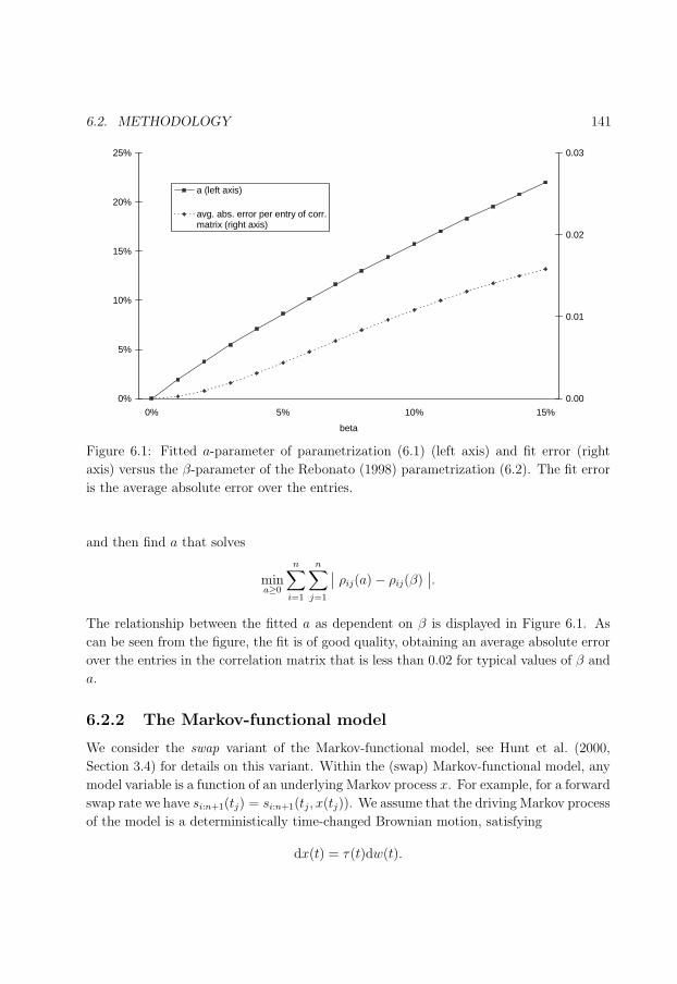
169


0%

5%

10%

15%

20%

25%

0% 5% 10% 15%

beta

0.00

0.01

0.02

0.03

a (left axis)

avg. abs. error per entry of corr.matrix (right axis)

Figure 6.1: Fitted a-parameter of parametrization (6.1) (left axis) and fit error (right

axis) versus the β-parameter of the Rebonato (1998) parametrization (6.2). The fit error

is the average absolute error over the entries.

and then find a that solves

mina≥0

n∑i=1

n∑j=1

∣∣ ρij(a)− ρij(β)∣∣.

The relationship between the fitted a as dependent on β is displayed in Figure 6.1. As

can be seen from the figure, the fit is of good quality, obtaining an average absolute error

over the entries in the correlation matrix that is less than 0.02 for typical values of β and

a.

6.2.2 The Markov-functional model

We consider the swap variant of the Markov-functional model, see Hunt et al. (2000,

Section 3.4) for details on this variant. Within the (swap) Markov-functional model, any

model variable is a function of an underlying Markov process x. For example, for a forward

swap rate we have si:n+1(tj) = si:n+1(tj, x(tj)). We assume that the driving Markov process

of the model is a deterministically time-changed Brownian motion, satisfying

dx(t) = τ(t)dw(t).

170


Here τ(·) denotes a deterministic function (that can be chosen piece-wise constant) and

w denotes a Brownian motion.

We now present an approximate formula for the terminal correlation. An argu-

ment explaining the formula is given, and in a later section we investigate the accu-

racy of the approximating formula. By a Taylor expansion, we have ln si:n+1(ti, x) ≈s(0)i:n+1(ti) + s

(1)i:n+1(ti)x. Since correlation is unaltered by a linear transformation, the ter-

minal correlation of the swap rates is thus approximately equal to the terminal correlation

of the underlying Markov process,

ρ(

ln si:n+1(ti), ln sj:n+1(tj)) ≈ ρ

(x(ti), x(tj)

). (6.3)

By straightforward calculation, for i < j,

ρ(

x(ti), x(tj))

=Cov(x(ti), x(tj))√

Var(x(ti))Var(x(tj))=

√√√√∫ ti0

τ 2(t)dt∫ tj0

τ 2(t)dt. (6.4)

In fact, any functional of the Markov process can be linearized by a Taylor expansion

and, according to the argument above, would exhibit the same approximate terminal

correlation (6.4). The above theoretical argument is therefore not very strong. The

approximation however turns out to be accurate, as will be shown numerically in Section

6.4.

In principle, the Markov-functional model can thus be approximately fitted to the

terminal correlation by minimization of the fitting error given a market-implied or his-

torically estimated terminal correlation matrix. The parameters for this minimization

problem are for example the n parameters governing the piece-wise constant function

τ(·). For ease of exposition we will however restrict our attention to the case of mean

reversion, i.e. τ(t) = exp(at), with a denoting the mean reversion parameter, see Section

4 of Hunt et al. (2000). In this case we have, for i < j,

ρ(

x(ti), x(tj))

=

√e2ati − 1

e2atj − 1. (6.5)

To verify that the Markov-functional model is properly calibrated to terminal corre-

lation, in the swap market model this correlation is approximately calculated to be, from

(6.1), for i < j,

∫ ti0

σi:n+1(t)σj:n+1(t)ρij(t)dt√∫ ti0

σ2i:n+1(t)dt

∫ tj0

σ2j:n+1(t)dt

=σi:n+1σj:n+1ρijti√

σ2i:n+1tiσ

2j:n+1tj

= ρij

√titj

=

√e2ati − 1

e2atj − 1. (6.6)

The specification (6.1) of the instantaneous correlation of the swap market model was con-

structed such that the (approximate) terminal correlation (6.5) of the Markov-functional

171


model with mean reversion parameter a is equal to the (approximate) terminal correlation

(6.6) in the swap market model with parameter a. We note that this correspondence does

not necessarily hold for the LIBOR market model, though we nonetheless employ it in

the comparison tests.

6.2.3 Estimating Greeks for callable products in market models

The algorithm of Longstaff & Schwartz (2001) (LS) renders the numeraire relative payoff

along a simulated path discontinuously dependent on initial input. The discontinuity in

the LS algorithm stems from the estimated optimal exercise index chosen from a discrete

set of possible exercise opportunities. Such a discrete choice is inherently discontinuously

dependent on initial input. Any discontinuity in a simulation may cause finite difference

estimates of sensitivities to be less efficient, see Glasserman (2004, Section 7.1). We

describe two methods that enhance the efficiency of finite difference estimates, the second

of which is novel. These are:

(i) Finite differences with optimal perturbation size.

(ii) Constant exercise decision heuristic.

The two methods are discussed below in more detail. We denote by v the base value of

the derivative, i.e., the value of the derivative in the unperturbed model.

Method (i), the finite differences method is best described as the bump-and-revalue

approach. Initial market data is perturbed by amount ε, the model is re-calibrated and

subsequently priced at v(ε). The finite difference estimate of the Greek is then (v(ε) −v)/ε. The mean square error (MSE) of the finite difference estimator is dependent on the

chosen perturbation size ε. If the numeraire relative payoff along the path is continuously

dependent on initial input, then least MSE is obtained when ε is selected as small as

possible (though larger than machine precision), see Glasserman (2004). If the payoff

is discontinuous however, then there is a trade-off between increasing and decreasing

ε, leading to an optimal (‘large’ and positive) choice of ε that attains least MSE, see

Glasserman (2004). After some preliminary testing, we found perturbation sizes of roughly

1 basis point (bp, 0.01%) for delta and 5 bp for vega.

Method (ii) that we propose, is named the constant exercise decision method. Here,

for the base valuation we record per path when the exercise decision takes place. In the

perturbed model, we no longer perform LS least-squares Monte Carlo, but rather use the

very same exercise strategy as in the base valuation case. The constant exercise boundary

method is a heuristic, since its estimate is stable but biased. The bias stems from not

taking into account the change in value of the derivative as a result of a change in the

(approximate) exercise decision. The bias is likely to be small, because the exercise deci-

sion is close to optimal by construction. Therefore, the change in value due to a change

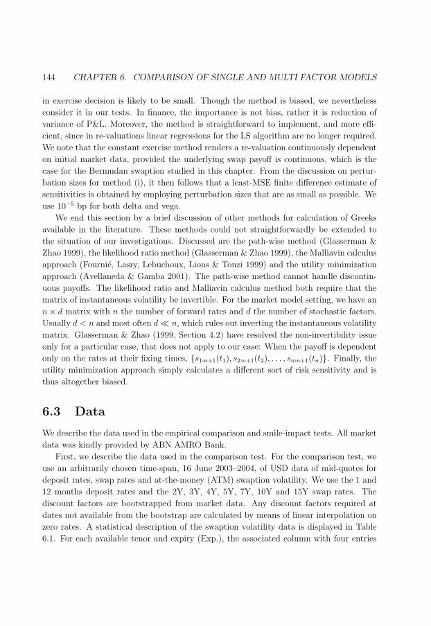
172


in exercise decision is likely to be small. Though the method is biased, we nevertheless

consider it in our tests. In finance, the importance is not bias, rather it is reduction of

variance of P&L. Moreover, the method is straightforward to implement, and more effi-

cient, since in re-valuations linear regressions for the LS algorithm are no longer required.

We note that the constant exercise method renders a re-valuation continuously dependent

on initial market data, provided the underlying swap payoff is continuous, which is the

case for the Bermudan swaption studied in this chapter. From the discussion on pertur-

bation sizes for method (i), it then follows that a least-MSE finite difference estimate of

sensitivities is obtained by employing perturbation sizes that are as small as possible. We

use 10−5 bp for both delta and vega.

We end this section by a brief discussion of other methods for calculation of Greeks

available in the literature. These methods could not straightforwardly be extended to

the situation of our investigations. Discussed are the path-wise method (Glasserman &

Zhao 1999), the likelihood ratio method (Glasserman & Zhao 1999), the Malliavin calculus

approach (Fournie, Lasry, Lebuchoux, Lions & Touzi 1999) and the utility minimization

approach (Avellaneda & Gamba 2001). The path-wise method cannot handle discontin-

uous payoffs. The likelihood ratio and Malliavin calculus method both require that the

matrix of instantaneous volatility be invertible. For the market model setting, we have an

n× d matrix with n the number of forward rates and d the number of stochastic factors.

Usually d < n and most often d ¿ n, which rules out inverting the instantaneous volatility

matrix. Glasserman & Zhao (1999, Section 4.2) have resolved the non-invertibility issue

only for a particular case, that does not apply to our case: When the payoff is dependent

only on the rates at their fixing times, s1:n+1(t1), s2:n+1(t2), . . . , sn:n+1(tn). Finally, the

utility minimization approach simply calculates a different sort of risk sensitivity and is

thus altogether biased.

6.3 Data

We describe the data used in the empirical comparison and smile-impact tests. All market

data was kindly provided by ABN AMRO Bank.

First, we describe the data used in the comparison test. For the comparison test, we

use an arbitrarily chosen time-span, 16 June 2003–2004, of USD data of mid-quotes for

deposit rates, swap rates and at-the-money (ATM) swaption volatility. We use the 1 and

12 months deposit rates and the 2Y, 3Y, 4Y, 5Y, 7Y, 10Y and 15Y swap rates. The

discount factors are bootstrapped from market data. Any discount factors required at

dates not available from the bootstrap are calculated by means of linear interpolation on

zero rates. A statistical description of the swaption volatility data is displayed in Table

6.1. For each available tenor and expiry (Exp.), the associated column with four entries

173

6.3. DATA 145

Table 6.1: Statistical description of the swaption volatility data.

Tenor (Years)Exp. 1 2 3 4 5 7 10 15 30

1M 46.3 51.7 45.9 40.6 37.8 32.1 27.5 22.9 19.0(6.2) (6.4) (6.2) (5.0) (4.7) (3.8) (3.5) (3.0) (2.7)[34.3, [34.0, [30.3, [27.8, [26.2, [22.8, [19.6, [16.6, [13.6,65.8] 68.3] 62.1] 53.1] 48.7] 42.1] 37.4] 33.0] 27.6]

2M 45.8 50.6 44.9 40.0 37.3 31.9 27.4 22.9 19.0(4.8) (5.5) (5.3) (4.3) (4.1) (3.2) (2.9) (2.5) (2.2)[36.0, [34.0, [30.3, [27.8, [26.2, [23.0, [19.9, [16.9, [13.8,61.0] 63.5] 57.0] 50.1] 47.2] 39.4] 35.0] 30.9] 25.7]

3M 45.4 49.4 44.0 39.5 36.9 31.7 27.3 22.9 18.9(3.9) (4.9) (4.5) (3.9) (3.6) (2.8) (2.5) (2.1) (1.8)[36.0, [34.0, [30.0, [27.6, [26.0, [23.0, [19.8, [16.9, [13.7,57.7] 60.3] 54.1] 49.3] 46.3] 37.8] 32.6] 28.8] 23.8]

6M 48.0 46.5 41.2 37.2 34.9 30.4 26.6 22.3 18.6(4.3) (4.6) (4.1) (3.6) (3.4) (2.6) (2.1) (1.6) (1.3)[34.9, [33.1, [29.3, [27.1, [25.4, [22.7, [20.0, [17.1, [14.1,56.9] 56.8] 52.7] 47.6] 44.5] 37.0] 31.3] 25.5] 20.9]

1Y 46.0 41.0 36.5 33.5 31.7 28.3 25.1 21.4 17.9(5.0) (4.7) (3.9) (3.4) (3.2) (2.5) (2.0) (1.5) (1.2)[32.1, [29.4, [27.0, [25.2, [23.7, [21.6, [19.5, [16.7, [14.2,55.5] 55.5] 48.2] 43.3] 40.6] 34.8] 30.0] 24.4] 20.3]

2Y 36.7 33.0 30.3 28.5 27.1 25.0 22.6 19.6 16.8(4.3) (3.7) (3.1) (2.8) (2.6) (2.2) (1.8) (1.5) (1.2)[26.9, [24.7, [23.2, [22.1, [21.1, [19.7, [17.9, [15.6, [13.5,50.4] 44.3] 39.4] 36.5] 34.5] 30.8] 27.1] 22.7] 19.5]

3Y 29.9 27.8 26.3 25.0 24.0 22.4 20.5 18.0 15.5(3.1) (2.7) (2.4) (2.2) (2.1) (1.8) (1.6) (1.3) (1.1)[23.2, [21.7, [20.7, [20.0, [19.3, [18.1, [16.6, [14.6, [12.7,38.6] 34.9] 32.6] 30.9] 29.7] 27.1] 24.2] 20.6] 18.1]

4Y 25.7 24.5 23.4 22.5 21.7 20.4 18.8 16.6 14.3(2.2) (2.1) (1.9) (1.8) (1.7) (1.5) (1.3) (1.1) (1.0)[20.8, [19.8, [19.1, [18.4, [17.9, [16.9, [15.6, [13.7, [11.9,31.0] 29.6] 28.2] 27.2] 26.4] 24.4] 22.0] 19.0] 16.9]

5Y 23.2 22.3 21.4 20.7 19.9 18.8 17.4 15.5 13.4(1.8) (1.7) (1.6) (1.6) (1.5) (1.3) (1.2) (1.0) (1.0)[19.1, [18.4, [17.8, [17.2, [16.7, [15.8, [14.7, [12.9, [11.2,28.0] 26.7] 25.7] 24.8] 24.0] 22.3] 20.2] 17.7] 15.8]

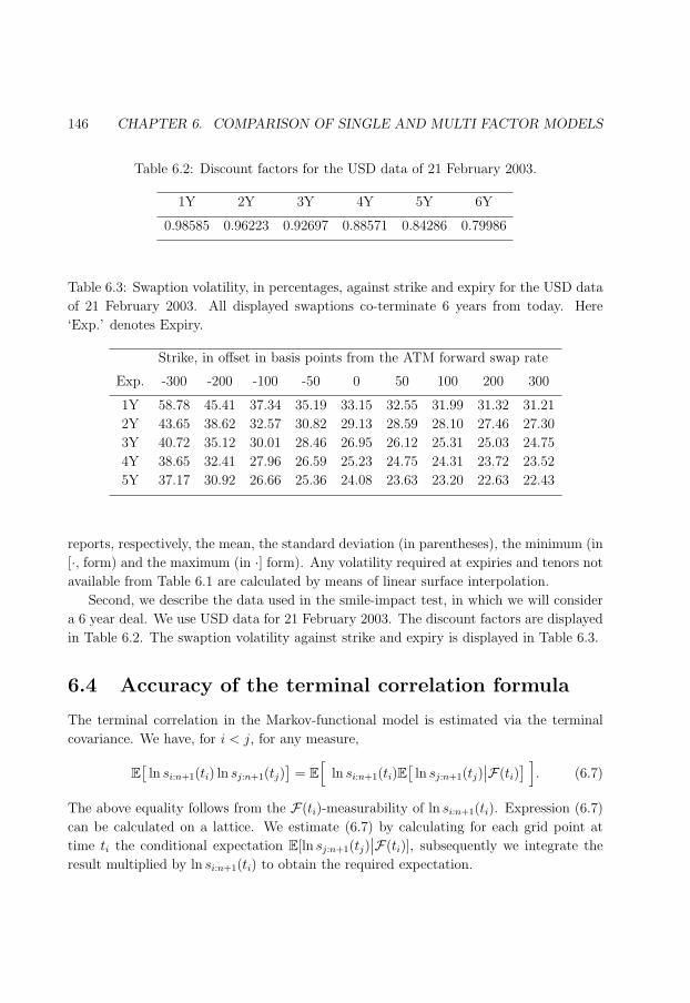
174


Table 6.2: Discount factors for the USD data of 21 February 2003.

1Y 2Y 3Y 4Y 5Y 6Y

0.98585 0.96223 0.92697 0.88571 0.84286 0.79986

Table 6.3: Swaption volatility, in percentages, against strike and expiry for the USD data

of 21 February 2003. All displayed swaptions co-terminate 6 years from today. Here

‘Exp.’ denotes Expiry.

Strike, in offset in basis points from the ATM forward swap rate

Exp. -300 -200 -100 -50 0 50 100 200 300

1Y 58.78 45.41 37.34 35.19 33.15 32.55 31.99 31.32 31.21

2Y 43.65 38.62 32.57 30.82 29.13 28.59 28.10 27.46 27.30

3Y 40.72 35.12 30.01 28.46 26.95 26.12 25.31 25.03 24.75

4Y 38.65 32.41 27.96 26.59 25.23 24.75 24.31 23.72 23.52

5Y 37.17 30.92 26.66 25.36 24.08 23.63 23.20 22.63 22.43

reports, respectively, the mean, the standard deviation (in parentheses), the minimum (in

[·, form) and the maximum (in ·] form). Any volatility required at expiries and tenors not

available from Table 6.1 are calculated by means of linear surface interpolation.

Second, we describe the data used in the smile-impact test, in which we will consider

a 6 year deal. We use USD data for 21 February 2003. The discount factors are displayed

in Table 6.2. The swaption volatility against strike and expiry is displayed in Table 6.3.

6.4 Accuracy of the terminal correlation formula

The terminal correlation in the Markov-functional model is estimated via the terminal

covariance. We have, for i < j, for any measure,

E[ln si:n+1(ti) ln sj:n+1(tj)

]= E

[ln si:n+1(ti)E

[ln sj:n+1(tj)

∣∣F(ti)] ]

. (6.7)

The above equality follows from the F(ti)-measurability of ln si:n+1(ti). Expression (6.7)

can be calculated on a lattice. We estimate (6.7) by calculating for each grid point at

time ti the conditional expectation E[ln sj:n+1(tj)∣∣F(ti)], subsequently we integrate the

result multiplied by ln si:n+1(ti) to obtain the required expectation.

175

6.5. EMPIRICAL COMPARISON RESULTS 147

Table 6.4: Error analysis of the terminal correlation measured in the Markov-functional

model versus given by the approximate formula (6.3), for a 40 years annual-paying deal,

thus for a 40 × 40 correlation matrix. Abbreviations used are m.r. for mean reversion,

max. for maximum, abs. for absolute, err. for error, rel. for relative, and avg. for average.

M.r. Max. abs. err. Max. rel. err. Avg. abs. err. Avg. rel. err.

0% 1.6× 10−4 0.0190% 4.5× 10−5 0.0076%

5% 5.0× 10−5 0.0072% 1.2× 10−5 0.0030%

10% 2.1× 10−5 0.0032% 3.0× 10−6 0.0012%

15% 1.0× 10−5 0.0018% 9.8× 10−7 0.0006%

20% 5.7× 10−6 0.0011% 4.0× 10−7 0.0003%

The accuracy of the approximate formula (6.3) is tested for a 40 years deal, with EUR

market data of 8 February 1999, for which the swaption volatility level is on average 14%.

The test is performed at various mean reversion levels, 0%, 5%, 10%, 15%, and 20%. The

terminal correlation matrix within the Markov-functional model is calculated numerically

on a lattice under the terminal measure and subsequently compared to the correlation

matrix given by the approximate formula (6.3). We note that the comparison contains two

sources of error: First, the approximation (6.3), and, second, the numerical error inherent

in the lattice calculation. In Table 6.4, various descriptive data for the comparison test

are displayed. Reported are, over the entries in the matrix, the maximum absolute and

relative errors, and the average absolute and relative errors. As can be seen from Table

6.4, these errors are quite small, especially considered over a 40 years horizon.

6.5 Empirical comparison results

In this section, we report the results of our empirical comparison. The deal description

is given in Table 6.5. For market models we use the terminal measure, 10,000 simulation

paths (5,000 plus 5,000 antithetic) and 10 stochastic factors (a full factor model), bar

when a = 0%, we use a single factor model. To determine the exercise boundary in

market models, we use the least-squares Monte Carlo algorithm of Longstaff & Schwartz

(2001), with all forward rates as explanatory variables, i.e., all available LIBOR rates

for the LIBOR market model and all available swap rates for the swap market model.

The reason for using all available rates as explanatory variables is that the multi factor

nature of the market models needs be retained (if at all present; for a = 0% a single

factor model must be used). As basis functions we use a constant and one linear term

176


Table 6.5: The Bermudan swaption deal used in the comparison.

Trade: Bermudan Swaption

Trade Type: Receive Fixed

Notional: USD 100m

Start Date: 16-Jun-2004

End Date: 16-Jun-2014

Fixed Rate: 3.2%

Index Coupon: Per Annum

Index Basis: ACT/365

Roll Type: Modified Following

Callable: At Fixing Dates

per explanatory variable, 1, x1, . . . , xm, where m denotes the number of explanatory

variables. The NPVs, deltas and vegas of the deal are calculated at each trade date

from 16 June 2003 till 15 June 2004, inclusive, for the mean reversion levels 0%, 5% and

10%. A price comparison is displayed in Figure 6.2. As can be seen from the figure, the

Markov-functional and market models are similar in terms of NPV, and prices co-move

and stay together over time.

The models are, more importantly, compared in terms of hedge performance. With

respect to hedging, we use so-called bucket hedging rather than factor hedging. With

factor hedging, the number of hedge instruments equals the number of factors in the

model. Risk sensitivities are calculated by perturbing only the model intrinsic factors.

With bucket hedging, the number of hedge instruments equals the number of market

traded instruments to which the model has been calibrated to. Risk sensitivities are

calculated by perturbing the value of a market traded asset, and then by re-valuation of

the derivative in a model re-calibrated to the perturbed market data. The reasons that

we employ bucket hedging rather than factor hedging are twofold. First, Driessen et al.

(2003, Section VII.C) show that bucket hedging outperforms factor hedging for caps and

European swaptions (for delta hedging). Second, bucket hedging corresponds to financial

practice.

Two types of hedges are considered:

(i) Delta hedging only.

(ii) Delta and vega hedging.

The delta hedge is set up in terms of discount bonds, one discount bond for each tenor

time associated with the deal. In the case of the deal of Table 6.5, there are 11 such

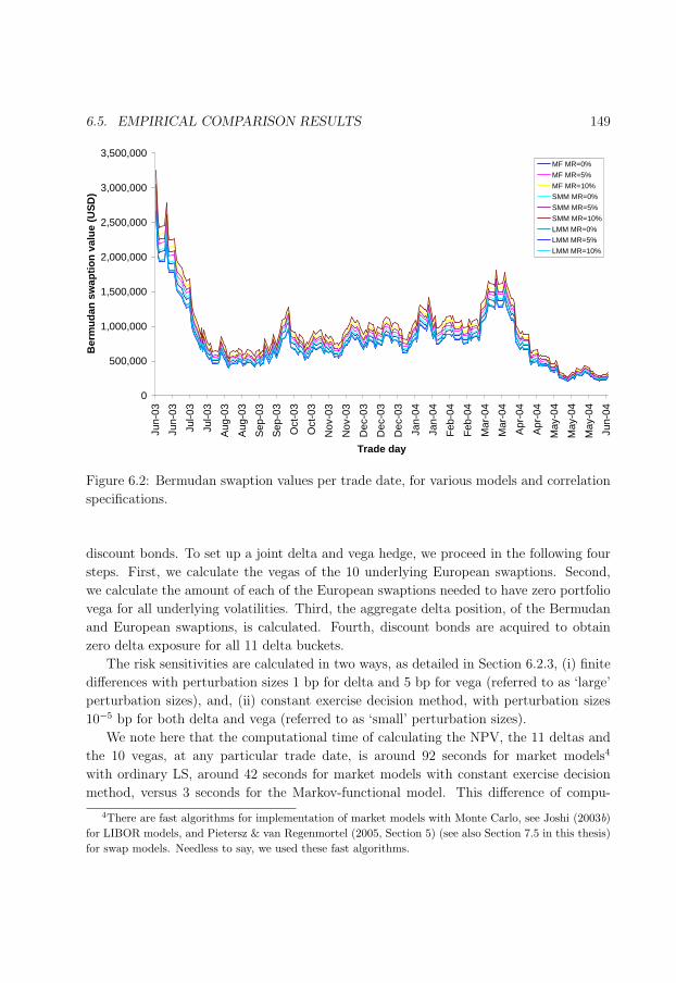
177


0

500,000

1,000,000

1,500,000

2,000,000

2,500,000

3,000,000

3,500,000Ju

n-03

Jun-

03

Jul-0

3

Jul-0

3

Aug

-03

Aug

-03

Sep

-03

Sep

-03

Oct

-03

Oct

-03

Nov

-03

Nov

-03

Dec

-03

Dec

-03

Dec

-03

Jan-

04

Jan-

04

Feb

-04

Feb

-04

Mar

-04

Mar

-04

Apr

-04

Apr

-04

May

-04

May

-04

May

-04

Jun-

04

Trade day

Ber

mu

dan

sw

apti

on

val

ue

(US

D)

MF MR=0%

MF MR=5%

MF MR=10%

SMM MR=0%

SMM MR=5%

SMM MR=10%

LMM MR=0%

LMM MR=5%

LMM MR=10%

Figure 6.2: Bermudan swaption values per trade date, for various models and correlation

specifications.

discount bonds. To set up a joint delta and vega hedge, we proceed in the following four

steps. First, we calculate the vegas of the 10 underlying European swaptions. Second,

we calculate the amount of each of the European swaptions needed to have zero portfolio

vega for all underlying volatilities. Third, the aggregate delta position, of the Bermudan

and European swaptions, is calculated. Fourth, discount bonds are acquired to obtain

zero delta exposure for all 11 delta buckets.

The risk sensitivities are calculated in two ways, as detailed in Section 6.2.3, (i) finite

differences with perturbation sizes 1 bp for delta and 5 bp for vega (referred to as ‘large’

perturbation sizes), and, (ii) constant exercise decision method, with perturbation sizes

10−5 bp for both delta and vega (referred to as ‘small’ perturbation sizes).

We note here that the computational time of calculating the NPV, the 11 deltas and

the 10 vegas, at any particular trade date, is around 92 seconds for market models4

with ordinary LS, around 42 seconds for market models with constant exercise decision

method, versus 3 seconds for the Markov-functional model. This difference of compu-

4There are fast algorithms for implementation of market models with Monte Carlo, see Joshi (2003b)for LIBOR models, and Pietersz & van Regenmortel (2005, Section 5) (see also Section 7.5 in this thesis)for swap models. Needless to say, we used these fast algorithms.

178


-500,000

-400,000

-300,000

-200,000

-100,000

0

100,000

200,000

300,000

400,000

MF 0%

(unhedged)

MF 0%

(delta

hedged)

MF 0%

(delta &

vega

hedged)

SMM 5%

(unhedged)

SMM 5%

(delta

hedged)

SMM 5%

(delta &

vega

hedged)

LMM 10%

(unhedged)

LMM 10%

(delta

hedged)

LMM 10%

(delta &

vega

hedged)

1st qrtmin

medianmax3rd qrt

Figure 6.3: Comparison of delta versus delta and vega hedging. Box-whisker plots for

the change in value (in USD) of the hedged portfolio. The percentages denote the mean

reversion level (MF) or correlation parametrization parameter (LMM and SMM). For

market models, we use the constant exercise decision method, with ‘small’ perturbation

sizes.

tational time is inherent to the (least squares) Monte Carlo implementation of market

models versus the lattice implementation of Markov-functional models. Of course, such

lattice implementation is allowed only because of the mild path-dependency of Bermudan

swaptions.

The hedge portfolios are set up at each trade day and the change in portfolio value on

the next trade day is recorded. The hedge test results are ordered in three subsections.

6.5.1 Delta hedging versus delta and vega hedging

The performance of delta hedging versus delta and vega hedging is compared. Box-whisker

plots, for the change in hedge portfolio value, are displayed in Figure 6.3, for various

models and mean reversion or correlation parametrization parameters. Here, MF, LMM,

and SMM denote respectively, Markov-functional model, LIBOR market model and swap

market model. Box-whisker plots provide a convenient representation of a distribution,

by displaying five of its key characteristics: the minimum, median, and maximum values,

and the first and third quartiles.

We draw the following conclusions from the box-whisker plots in Figure 6.3:

1. Delta hedging significantly decreases variance of P&L.

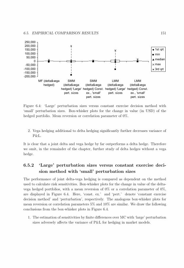
179


-200,000

-150,000

-100,000

-50,000

0

50,000

100,000

150,000

200,000

250,000

MF (delta&vega

hedged)

SMM

(delta&vega

hedged) 'Large'

pert. sizes

SMM

(delta&vega

hedged) Const.

ex., 'small'

pert. sizes

LMM

(delta&vega

hedged) 'Large'

pert. sizes

LMM

(delta&vega

hedged) Const.

ex., 'small'

pert. sizes

1st qrt

min

median

max

3rd qrt

Figure 6.4: ‘Large’ perturbation sizes versus constant exercise decision method with

‘small’ perturbation sizes. Box-whisker plots for the change in value (in USD) of the

hedged portfolio. Mean reversion or correlation parameter of 0%.

2. Vega hedging additional to delta hedging significantly further decreases variance of

P&L.

It is clear that a joint delta and vega hedge by far outperforms a delta hedge. Therefore

we omit, in the remainder of the chapter, further study of delta hedges without a vega

hedge.

6.5.2 ‘Large’ perturbation sizes versus constant exercise deci-

sion method with ‘small’ perturbation sizes

The performance of joint delta-vega hedging is compared as dependent on the method

used to calculate risk sensitivities. Box-whisker plots for the change in value of the delta-

vega hedged portfolios, with a mean reversion of 0% or a correlation parameter of 0%,

are displayed in Figure 6.4. Here, ‘const. ex.’ and ‘pert.’ denote ‘constant exercise

decision method’ and ‘perturbation’, respectively. The analogous box-whisker plots for

mean reversion or correlation parameters 5% and 10% are similar. We draw the following

conclusions from the box-whisker plots in Figure 6.4.

1. The estimation of sensitivities by finite differences over MC with ‘large’ perturbation

sizes adversely affects the variance of P&L for hedging in market models.

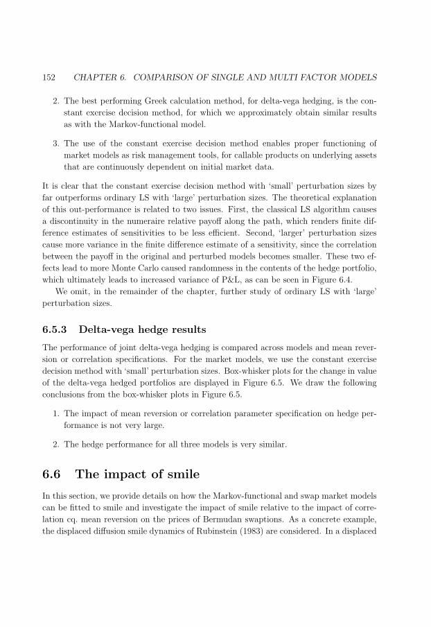
180


2. The best performing Greek calculation method, for delta-vega hedging, is the con-

stant exercise decision method, for which we approximately obtain similar results

as with the Markov-functional model.

3. The use of the constant exercise decision method enables proper functioning of

market models as risk management tools, for callable products on underlying assets

that are continuously dependent on initial market data.

It is clear that the constant exercise decision method with ‘small’ perturbation sizes by

far outperforms ordinary LS with ‘large’ perturbation sizes. The theoretical explanation

of this out-performance is related to two issues. First, the classical LS algorithm causes

a discontinuity in the numeraire relative payoff along the path, which renders finite dif-

ference estimates of sensitivities to be less efficient. Second, ‘larger’ perturbation sizes

cause more variance in the finite difference estimate of a sensitivity, since the correlation

between the payoff in the original and perturbed models becomes smaller. These two ef-

fects lead to more Monte Carlo caused randomness in the contents of the hedge portfolio,

which ultimately leads to increased variance of P&L, as can be seen in Figure 6.4.

We omit, in the remainder of the chapter, further study of ordinary LS with ‘large’

perturbation sizes.

6.5.3 Delta-vega hedge results

The performance of joint delta-vega hedging is compared across models and mean rever-

sion or correlation specifications. For the market models, we use the constant exercise

decision method with ‘small’ perturbation sizes. Box-whisker plots for the change in value

of the delta-vega hedged portfolios are displayed in Figure 6.5. We draw the following

conclusions from the box-whisker plots in Figure 6.5.

1. The impact of mean reversion or correlation parameter specification on hedge per-

formance is not very large.

2. The hedge performance for all three models is very similar.

6.6 The impact of smile

In this section, we provide details on how the Markov-functional and swap market models

can be fitted to smile and investigate the impact of smile relative to the impact of corre-

lation cq. mean reversion on the prices of Bermudan swaptions. As a concrete example,

the displaced diffusion smile dynamics of Rubinstein (1983) are considered. In a displaced

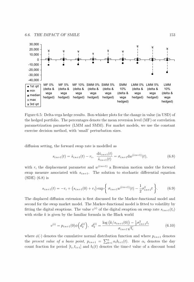
181

6.6. THE IMPACT OF SMILE 153

-40,000

-30,000

-20,000

-10,000

0

10,000

20,000

30,000

MF 0%

(delta &

vega

hedged)

MF 5%

(delta &

vega

hedged)

MF 10%

(delta &

vega

hedged)

SMM 0%

(delta &

vega

hedged)

SMM 5%

(delta &

vega

hedged)

SMM

10%

(delta &

vega

hedged)

LMM 0%

(delta &

vega

hedged)

LMM 5%

(delta &

vega

hedged)

LMM

10%

(delta &

vega

hedged)

1st qrt

min

median

max

3rd qrt

Figure 6.5: Delta-vega hedge results. Box-whisker plots for the change in value (in USD) of

the hedged portfolio. The percentages denote the mean reversion level (MF) or correlation

parametrization parameter (LMM and SMM). For market models, we use the constant

exercise decision method, with ‘small’ perturbation sizes.

diffusion setting, the forward swap rate is modelled as

si:n+1(t) = si:n+1(t)− ri,dsi:n+1(t)

si:n+1(t)= σi:n+1dw(i:n+1)(t), (6.8)

with ri the displacement parameter and w(i:n+1) a Brownian motion under the forward

swap measure associated with si:n+1. The solution to stochastic differential equation

(SDE) (6.8) is

si:n+1(t) = −ri +(si:n+1(0) + ri

)exp

σi:n+1w

(i:n+1)(t)− 1

2σ2

i:n+1t

. (6.9)

The displaced diffusion extension is first discussed for the Markov-functional model and

second for the swap market model. The Markov-functional model is fitted to volatility by

fitting the digital swaptions. The value v(i) of the digital swaption on swap rate si:n+1(ti)

with strike k is given by the familiar formula in the Black world

v(i) = pi:n+1(0)φ(d

(i)2

), d

(i)2 =

log(k/si:n+1(0)

)− 12σ2

i:n+1ti

σi:n+1

√ti

(6.10)

where φ(·) denotes the cumulative normal distribution function and where pi:n+1 denotes

the present value of a basis point, pi:n+1 =∑n

k=i αibi+1(t). Here αi denotes the day

count fraction for period [ti, ti+1] and bi(t) denotes the time-t value of a discount bond

182


for payment of one unit of currency at time ti. In the displaced diffusion world, the value

v(i) of the digital swaption is given by a displaced forward swap rate and strike

v(i) = pi:n+1(0)φ(d

(i)2

), d

(i)2 =

log(

si:n+1(0)+ri

k+ri

)− 1

2σ2

i:n+1ti

σi:n+1

√ti

. (6.11)

The implementation of a non-smile Markov-functional model has to be changed only in

two places to incorporate displaced diffusion smile dynamics. First, the functional form

of the terminal discount bond bn+1 at time tn is determined, using the equation

bn+1(tn) =1

1 + αnsn:n+1(tn). (6.12)

In a non-smile Markov-functional model, we then have

bn+1(tn, x(tn)) =1

1 + αnsn:n+1(0) exp− 1

2σ2

n:n+1tn + σn:n+1

e2atn−1x(tn)

, (6.13)

this is exactly the penultimate equation on page 399 of Hunt et al. (2000). In a displaced

diffusion setting, we substitute (6.9) into (6.12) and then (6.13) becomes

bn+1(tn, x(tn)) =1

1 + αn

[− ri +

(sn:n+1(0) + ri

)exp

− 12σ2

n:n+1tn + σn:n+1

e2atn−1x(tn)

] ,

Second, the functional forms of the swap rates si:n+1(ti, ·), i = 1, . . . , n−1 are determined,

by inverting the value of the digital swaption against strike. In a non-smile Markov-

functional model, we invert (6.10) and obtain

si:n+1(ti, x(ti)) = si:n+1(0) exp

− 1

2σ2

i:n+1ti − σi:n+1

√tiφ

−1

(j(i)(x(ti))

pi:n+1(0)

),

with j(i)(x) denoting the value of a digital swaption with strike x in the model, calculated

by induction from i = n − 1, . . . , 1. In a displaced diffusion setting, we invert (6.11) to

obtain

si:n+1(ti, x(ti)) = −ri +(si:n+1(0) + ri

)exp

− 1

2σ2

i:n+1ti − σi:n+1

√tiφ

−1

(j(i)(x(ti))

pi:n+1(0)

).

Next, the displaced diffusion swap market model is made reference to. The dynamics

of the forward swap rates under the terminal measure in general smile models can be

found in Jamshidian (1997, Equation (6), page 320).

We fit the displaced diffusion model to the market data of Table 6.3 and find the

volatility parameters σi:n+1 and displacement parameters ri as listed in Table 6.6. The

fitted volatility and fit errors are displayed in Table 6.7. As can be seen from the table,

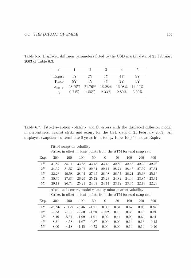
183


Table 6.6: Displaced diffusion parameters fitted to the USD market data of 21 February

2003 of Table 6.3.

i 1 2 3 4 5

Expiry 1Y 2Y 3Y 4Y 5Y

Tenor 5Y 4Y 3Y 2Y 1Y

σi:n+1 28.29% 21.76% 18.28% 16.08% 14.62%

ri 0.71% 1.55% 2.33% 2.89% 3.39%

Table 6.7: Fitted swaption volatility and fit errors with the displaced diffusion model,

in percentages, against strike and expiry for the USD data of 21 February 2003. All

displayed swaptions co-terminate 6 years from today. Here ‘Exp.’ denotes Expiry.

Fitted swaption volatilityStrike, in offset in basis points from the ATM forward swap rate

Exp. -300 -200 -100 -50 0 50 100 200 300

1Y 37.82 35.11 33.88 33.48 33.15 32.89 32.66 32.30 32.032Y 34.32 31.57 30.07 29.54 29.11 28.74 28.43 27.92 27.513Y 32.23 29.58 28.02 27.45 26.98 26.57 26.21 25.63 25.164Y 30.34 27.83 26.29 25.72 25.23 24.82 24.46 23.85 23.375Y 29.17 26.74 25.21 24.63 24.14 23.72 23.35 22.73 22.23

Absolute fit errors, model volatility minus market volatilityStrike, in offset in basis points from the ATM forward swap rate

Exp. -300 -200 -100 -50 0 50 100 200 300

1Y -20.96 -10.29 -3.46 -1.71 0.00 0.34 0.67 0.98 0.822Y -9.33 -7.05 -2.50 -1.28 -0.02 0.15 0.33 0.45 0.213Y -8.49 -5.54 -1.99 -1.01 0.02 0.44 0.90 0.60 0.414Y -8.31 -4.58 -1.67 -0.87 0.00 0.06 0.14 0.13 -0.155Y -8.00 -4.18 -1.45 -0.73 0.06 0.09 0.14 0.10 -0.20

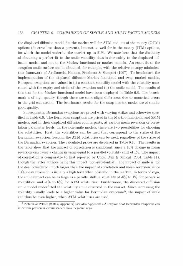
184


the displaced diffusion model fits the market well for ATM and out-of-the-money (OTM)

options (fit error less than a percent), but not so well for in-the-money (ITM) options,

for which the model underfits the market up to 21%. We note here that the disability

of obtaining a perfect fit to the smile volatility data is due solely to the displaced dif-

fusion model, and not to the Markov-functional or market models. An exact fit to the

swaption smile surface can be obtained, for example, with the relative-entropy minimiza-

tion framework of Avellaneda, Holmes, Friedman & Samperi (1997). To benchmark the

implementation of the displaced diffusion Markov-functional and swap market models,

European swaptions are valued in (i) a constant volatility model with the volatility asso-

ciated with the expiry and strike of the swaption and (ii) the smile model. The results of

this test for the Markov-functional model have been displayed in Table 6.8. The bench-

mark is of high quality, though there are some slight differences due to numerical errors

in the grid calculation. The benchmark results for the swap market model are of similar

good quality.

Subsequently, Bermudan swaptions are priced with varying strikes and otherwise spec-

ified in Table 6.9. The Bermudan swaptions are priced in the Markov-functional and SMM

models, and in their displaced diffusion counterparts, at various mean reversion or corre-

lation parameter levels. In the non-smile models, there are two possibilities for choosing

the volatilities. First, the volatilities can be used that correspond to the strike of the

Bermudan swaption. Second, the ATM volatilities can be used, regardless of the strike of

the Bermudan swaption. The calculated prices are displayed in Table 6.10. The results in

the table show that the impact of correlation is significant, since a 10% change in mean

reversion can cause a change in value equal to a parallel volatility shift of 1%. The impact

of correlation is comparable to that reported by Choy, Dun & Schlogl (2004, Table 11),

though the latter authors name this impact ‘non-substantial’. The impact of smile is, for

the deal considered, much larger than the impact of correlation and mean reversion, since

10% mean reversion is usually a high level when observed in the market. In terms of vega,

the smile impact can be as large as a parallel shift in volatility of -8% to 1%, for per-strike

volatilities, and -1% to 6%, for ATM volatilities. Furthermore, the displaced diffusion

smile model underfitted the volatility smile observed in the market. Since increasing the

volatility usually leads to a higher value for Bermudan swaptions5, the impact of smile

can thus be even higher, when ATM volatilities are used.

5Pietersz & Pelsser (2004a, Appendix) (see also Appendix 2.A) explain that Bermudan swaptions canin certain particular circumstances have negative vega.

185


Tab

le6.

8:B

ench

mar

kre

sult

sfo

rth

edis

pla

ced

diff

usi

onM

arko

v-funct

ional

model

:E

uro

pea

nsw

apti

onpri

cesin

aco

nst

ant

vola

tility

model

vers

us

asm

ile

model

.T

he

not

ional

isU

SD

100

million

.A

lldis

pla

yed

swap

tion

sco

-ter

min

ate

6ye

ars

from

today

.H

ere

‘Exp.’

den

otes

Expir

y.

Str

ike,

inoff

set

inbas

ispoi

nts

from

the

AT

Mfo

rwar

dsw

apra

te

-300

-200

-100

-50

050

100

200

300

Exp.

Con

stan

tvo

lati

lity

Mar

kov-funct

ional

model

1Y32

852

,561

606,

777

1,30

4,85

12,

340,

174

3,68

9,48

55,

298,

889

9,05

3,75

713

,203

,090

2Y24

,540

249,

639

1,01

8,21

31,

683,

785

2,54

2,75

93,

580,

442

4,77

3,68

57,

521,

975

10,5

95,4

80

3Y84

,026

391,

072

1,09

8,96

51,

629,

508

2,27

6,28

53,

030,

862

3,88

1,50

45,

818,

070

7,98

4,79

9

4Y10

6,95

936

7,45

787

8,15

61,

237,

121

1,66

3,27

42,

151,

967

2,69

7,07

33,

928,

998

5,30

5,39

4

5Y82

,725

235,

077

504,

020

684,

928

895,

662

1,13

4,22

51,

398,

093

1,99

0,49

72,

650,

706

Dis

pla

ced

diff

usi

onM

arko

v-funct

ional

model

1Y32

252

,255

605,

446

1,30

3,08

32,

338,

220

3,68

7,59

95,

297,

237

9,05

2,72

713

,202

,556

2Y24

,201

248,

060

1,01

5,12

41,

680,

221

2,53

8,99

33,

576,

743

4,77

0,23

87,

519,

330

10,5

93,6

75

3Y83

,169

388,

983

1,09

5,78

11,

626,

018

2,27

2,66

83,

027,

290

3,87

8,10

15,

815,

249

7,98

2,66

7

4Y10

5,99

036

5,58

887

5,58

61,

234,

362

1,66

0,43

32,

149,

153

2,69

4,36

63,

926,

683

5,30

3,55

0

5Y82

,154

234,

125

502,

792

683,

627

894,

329

1,13

2,90

31,

396,

815

1,98

9,37

82,

649,

787

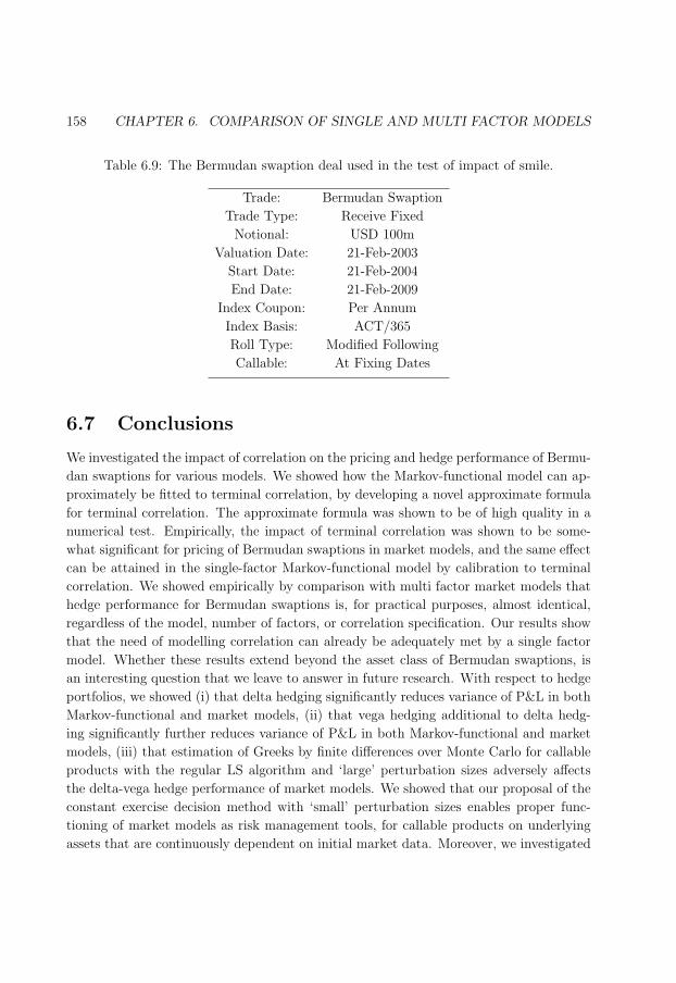
186


Table 6.9: The Bermudan swaption deal used in the test of impact of smile.

Trade: Bermudan Swaption

Trade Type: Receive Fixed

Notional: USD 100m

Valuation Date: 21-Feb-2003

Start Date: 21-Feb-2004

End Date: 21-Feb-2009

Index Coupon: Per Annum

Index Basis: ACT/365

Roll Type: Modified Following

Callable: At Fixing Dates

6.7 Conclusions

We investigated the impact of correlation on the pricing and hedge performance of Bermu-

dan swaptions for various models. We showed how the Markov-functional model can ap-

proximately be fitted to terminal correlation, by developing a novel approximate formula

for terminal correlation. The approximate formula was shown to be of high quality in a

numerical test. Empirically, the impact of terminal correlation was shown to be some-

what significant for pricing of Bermudan swaptions in market models, and the same effect

can be attained in the single-factor Markov-functional model by calibration to terminal

correlation. We showed empirically by comparison with multi factor market models that

hedge performance for Bermudan swaptions is, for practical purposes, almost identical,

regardless of the model, number of factors, or correlation specification. Our results show

that the need of modelling correlation can already be adequately met by a single factor

model. Whether these results extend beyond the asset class of Bermudan swaptions, is

an interesting question that we leave to answer in future research. With respect to hedge

portfolios, we showed (i) that delta hedging significantly reduces variance of P&L in both

Markov-functional and market models, (ii) that vega hedging additional to delta hedg-

ing significantly further reduces variance of P&L in both Markov-functional and market

models, (iii) that estimation of Greeks by finite differences over Monte Carlo for callable

products with the regular LS algorithm and ‘large’ perturbation sizes adversely affects

the delta-vega hedge performance of market models. We showed that our proposal of the

constant exercise decision method with ‘small’ perturbation sizes enables proper func-

tioning of market models as risk management tools, for callable products on underlying

assets that are continuously dependent on initial market data. Moreover, we investigated

187

6.7. CONCLUSIONS 159

Table 6.10: Prices of Bermudan swaptions in smile versus non-smile models with various

correlation/mean reversion assumptions. Here ‘MF’, ‘MR’, ‘a’ and ‘SE’ denote ‘Markov-

functional model’, ‘mean reversion’, ‘the correlation parameter a of (6.1)’ and the ‘stan-

dard error’, respectively. Any difference (‘Diff.’) is with respect to a price at zero mean

reversion or at zero a. The non-smile models use per-strike volatilities, except where

indicated that ATM volatilities are used.

Strike

2% 3% 4% 5% 6%

MF-MR=0% 420,954 1,072,043 2,452,060 5,047,951 8,573,535

Vega 1% MF 34,609 68,118 96,242 93,513 68,477

SMM-a=0% 407,667 1,053,210 2,443,332 5,065,794 8,605,508

SMM SE-a=0% 7,551 12,964 17,204 16,032 10,625

Vega 1% SMM 33,105 66,154 97,141 91,850 67,194

MF-MR=5% 436,518 1,103,269 2,495,689 5,090,486 8,606,769

Diff. in vega 0.4 0.5 0.5 0.5 0.5

SMM-a=5% 407,922 1,060,731 2,461,625 5,101,071 8,657,349

SMM SE-a=5% 7,386 12,764 17,228 16,244 11,243

Diff. in vega 0.0 0.1 0.2 0.4 0.8

MF-MR=10% 452,417 1,135,155 2,540,694 5,135,323 8,642,685

Diff. in vega 0.9 0.9 0.9 0.9 1.0

SMM-a=10% 405,819 1,062,986 2,485,969 5,142,268 8,708,570

SMM SE-a=10% 7,202 12,488 17,090 16,359 11,873

Diff. in vega -0.1 0.1 0.4 0.8 1.5

Smile MF 148,130 747,270 2,347,664 5,074,574 8,623,356

Diff. in vega -7.9 -4.8 -1.1 0.3 0.7

Smile SMM 146,223 756,925 2,373,545 5,094,288 8,642,666

Smile SMM SE 4,710 11,138 16,781 14,437 9,801

Diff. in vega -8.3 -4.8 -0.8 0.5 1.0

ATM volatilities

MF-MR=0% 67,210 650,483 2,328,235 5,124,154 8,691,466

Vega 1% MF 14,997 60,797 95,139 93,681 72,106

Smile MF 148,130 747,270 2,347,664 5,074,574 8,623,356

Diff. in vega 5.4 1.6 0.2 -0.5 -0.9

SMM-a=0% 61,944 610,939 2,286,869 5,139,345 8,731,084

SMM SE-a=0% 2,626 10,114 16,763 16,122 11,628

Vega 1% SMM 13,915 59,861 94,495 91,859 77,375

Smile SMM 146,223 756,925 2,373,545 5,094,288 8,642,666

Diff. in vega 6.1 2.4 0.9 -0.5 -1.1

188


the impact of smile via displaced diffusion versions of the Markov-functional and swap

market models. For a particular deal and USD market data, we showed that the impact

of smile is much larger that the impact of correlation.

189

Chapter 7

Generic market models

Currently, there are two market models for valuation and risk management of interest

rate derivatives, the LIBOR and swap market models of Brace et al. (1997), Jamshid-

ian (1997), Musiela & Rutkowski (1997) and Miltersen et al. (1997). In this chapter,

we introduce arbitrage-free constant maturity swap (CMS) market models and generic

market models featuring forward rates that span periods other than the classical LIBOR

and swap periods. The generic market model generalizes the LIBOR and swap market

models. We derive necessary and sufficient conditions for the structure of the forward

rates to span an arbitrage-free economy in terms of relative discount bond prices, at all

times. We develop generic expressions for the drift terms occurring in the stochastic dif-

ferential equation driving the forward rates under a single pricing measure. The generic

market model is particularly apt for pricing of Bermudan CMS swaptions, fixed-maturity

Bermudan swaptions, and callable hybrid coupon swaps. We show how the instantaneous

correlation of the generic forward rates can be calculated from the single instantaneous

correlation matrix of forward LIBOR rates. These results are sufficient for implementation

of calibration and pricing algorithms for generic market models.

7.1 Introduction

Generic market models are specifically designed for the pricing of certain types of swaps.

In particular, we will consider constant maturity swaps (CMS) and hybrid coupon swaps.

An interest rate swap is an agreement to exchange, over a specified period, interest rate

payments, at a specified frequency, over a specified underlying notional that is not ex-

changed. In a plain-vanilla swap, the floating interest rate is the LIBOR rate. A constant

maturity swap pays not the LIBOR rate but instead a swap rate with specified tenor, fixed

for all payments in the CMS swap. The payment frequency remains unchanged however.

A hybrid coupon swap is a swap that features a floating payment schedule, designating the

190

162 CHAPTER 7. GENERIC MARKET MODELS

nature of each of the floating payments. The nature of the floating payment can be that it

is determined by either a LIBOR rate with varying maturity or a swap rate with varying

tenor. An example of such a payment schedule has been given in Table 7.1. Additionally,

the function that transforms the LIBOR or swap rate into a cash flow may even be not

entirely linear, for example, capped, floored or inverse.

The above swaps may have the feature that the swaps can be cancelled. Such versions

are deemed cancellable swaps. To hold a cancellable swap is equal to holding a swap and

an option to enter into the very same swap but with reversed cash flows1. The latter

option is called a callable swap. In this chapter we will also be concerned with the pricing

of callable and cancellable CMS and hybrid coupon swaps. There are two types of callable

swaptions: fixed-maturity or co-terminal. A co-terminal option allows to enter into an

underlying swap at several exercise opportunities, where each swap ends at the same

contractually determined end date. The swap maturity becomes shorter as exercise is

delayed. In contrast, for the fixed-maturity version, each underlying swap has the same

contractually specified maturity and the respective end dates then differ.

The main outset of the chapter is that a model is deemed to be proper for valuing a

certain callable or cancellable swap, if the volatility of a rate that appears in the contract

payoff has been calibrated correctly to the market volatility. The concept is best illustrated

by example. In the case of the hybrid coupon swap of Table 7.1 at the valuation date 11

June 2004, we would want to calibrate exactly to the volatilities of the 1Y ×2Y swaption,

2Y × 4Y swaption, 3Y caplet, 4Y × 2Y swaption and 5Y caplet. In contrast, for a cap

one would calibrate to the volatilities of the 1Y , 2Y , 3Y , 4Y and 5Y caplets. For a

co-terminal Bermudan swaption, to the volatilities of the 1Y × 5Y , 2Y × 4Y , 3Y × 3Y ,

4Y × 2Y and 5Y × 1Y swaptions. When employing a LIBOR market model to value a

cap, the model would feature the following 1Y forward LIBOR rates: 1Y , 2Y , 3Y , 4Y

and 5Y . If a swap market model would be used to value the Bermudan swaption, it would

feature the 1Y × 5Y , 2Y × 4Y , 3Y × 3Y , 4Y × 2Y and 5Y × 1Y forward swap rates. For

both LIBOR and swap market models, the canonical interest rates are simply equipped

with the corresponding canonical volatilities, allowing for an efficient and straightforward

calibration. Obviously, to straightforwardly calibrate a market model for the hybrid

coupon swap of Table 7.1, and callable or cancellable versions thereof, the model would

have to feature the forward swap rates 1Y × 2Y , 2Y × 4Y , 4Y × 2Y , and the 1Y forward

LIBOR rates at 3Y and 5Y . Up to now, whether a model containing such rates would

be arbitrage-free is not well-known. To our knowledge, generic methods for deriving the

arbitrage-free drift terms for the SDE driving the various forward rates have not been

developed yet. In this chapter, we develop such generic theory.

1Some readers might not be familiar with ‘callable’ and ‘cancellable’ swaps and might prefer to thinkof swaps and options thereon.

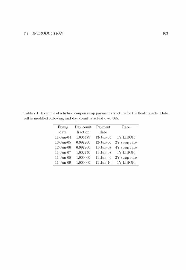
191


Table 7.1: Example of a hybrid coupon swap payment structure for the floating side. Date

roll is modified following and day count is actual over 365.

Fixing Day count Payment Rate

date fraction date

11-Jun-04 1.005479 13-Jun-05 1Y LIBOR

13-Jun-05 0.997260 12-Jun-06 2Y swap rate


11-Jun-07 1.002740 11-Jun-08 1Y LIBOR


11-Jun-09 1.000000 11-Jun-10 1Y LIBOR

192


In terms of practical relevance, the generic market model technology is valuable to

financial institutions that aim to trade in CMS Bermudan swaptions or callable hybrid

coupon swaps. As such, their costumers might require any sequence of various maturity

LIBOR or swap rate payments in the tailored exotic derivatives that they demand for

their business. In this chapter, we show that a generic implementation of the resulting

drift terms is feasible in practice, thereby enabling proper pricing and hedging of such

hybrid coupon swaps.

A further motivation for the theory in this chapter is that the idea of generic market

models is not new to the finance literature, since it has already been suggested by Gal-

luccio, Huang, Ly & Scaillet (2004). These authors discuss what they call the co-sliding

(commonly referred to as ‘LIBOR’) and co-terminal (commonly referred to as ‘swap’)

market models. The class of co-sliding market models corresponds to our class of CMS

market models, but ours is defined differently. Galluccio et al. (2004) show that the only

admissible co-sliding model is the LIBOR market model. Interestingly, we show that there

are n arbitrage-free CMS market models associated with a tenor structure with n fixings,

and the LIBOR and swap models are two special cases of these CMS models. In addi-

tion to the n CMS models, we introduce generic market models, extending the number

of arbitrage-free market models to n!. Also, Galluccio et al. (2004) discuss the co-initial

market model, but this model does not fit into our dynamic market model framework.

Moreover, in contrast to Galluccio et al. (2004), we derive generic expressions for the drift

terms of the forward rates, for all n! models (thus for LIBOR, swap, CMS and generic

models).

An alternative way of calibrating a model to the relevant volatility levels, is to take

a LIBOR market model, and derive generic approximate expressions for the volatility

of various forward rates. Such a procedure, for the specific case of calibration of the

LIBOR model to swaption volatility, has been investigated in Jackel & Rebonato (2003),

Joshi & Theis (2002), Hull & White (2000) and Pietersz & Pelsser (2004a) (Chapter 2).

The advantage of the generic market model specification is that the relevant volatility

functions can be directly specified. Moreover, the development of the theory of generic

market models is justified already by the additional insight into the workings of LIBOR

and swap market models. Also, Pietersz & Pelsser (2005a) (see also Chapter 6) provide

an empirical price and hedge comparison for Bermudan swaptions with either (i) the

LIBOR model calibrated to swaption volatility via the approximate formula, or (ii) the

swap model equipped with its canonical swaption volatility. Prices turn out to be largely

similar, while hedge performance seems to be slightly better for the canonical models, see

Figures 2 and 5, respectively, of Pietersz & Pelsser (2005a) (see Figures 6.2 and 6.5 of

this thesis). These results are thus slightly in favour of CMS and generic market models,

rather than the use of approximate swaption volatility with the LIBOR model.

193

7.2. PRELIMINARIES 165

We mention three areas of market model theory to which the generic market model

approach extends. First, generic models may also be used in multi-currency market

models, see Schlogl (2002). Second, a numerical implementation of a generic model may

utilize drift approximations, see, for example, Hunter et al. (2001) and Pietersz et al. (2004,

2005) (see also Chapter 5). Third, generic models may be equipped with smile dynamics.

The volatility smile is the phenomenon that for European options different Black (1976)

implied volatilities are quoted in the market when the strike of the option is varied. The

derivation of generic market models in this chapter does not make any assumptions on the

instantaneous volatility. As a result, smile-incorporating models, such as the displaced

diffusion (Rubinstein 1983), and constant elasticity of variance (CEV) (Cox & Ross 1976)

models, can be readily applied to the generic market model framework. An application of

the CEV specification to the LIBOR market model can be found in Andersen & Andreasen

(2000).

Finally, for an in-depth overview of pricing models for interest rate derivatives, the

reader is referred to Rebonato (2004a).

An outline of the chapter is as follows. First, preliminaries are introduced. Second,

necessary and sufficient no-arbitrage conditions on the structure and values of the forward

rates are derived. Third, generic arbitrage-free drift terms for the forward rates are derived

under a change of measure in a market model setting. Fourth, the numeric efficiency of

the generic drift term calculations is discussed. Fifth, the issue of calibrating generic

market models to correlation is addressed. Sixth, we end with conclusions.

7.2 Preliminaries

We consider tenor times or a tenor structure 0 =: t1 < · · · < tn+1 and day count fractions

αi, over the period [ti, ti+1], for i = 1, . . . , n. Suppose traded in the market is a set of m

forward LIBOR or swap rate agreements that are associated with that tenor structure2.

Initially, m may be different from n, but in Theorem 8 we show that it makes sense, from

an economic point of view, to consider only m = n. The set of associated forward swap

agreements is administered by a set of pairs

E =

εj =(s(j), e(j)

); j = 1, . . . , m ; s(j), e(j) integers 1 ≤ s(j) < e(j) ≤ n + 1

.

(7.1)

Here s(j) and e(j) denote start and end of the forward swap agreement. The above set

expression for E simply designates that there are m associated forward swap agreements,

that each forward swap agreement starts and ends on one of the tenor times and that a

2The frequency of the floating payments is restricted to one payment per fixed-payment period, butthis is only for ease of exposition. In practice, this assumption may be relaxed and the theory followsthrough unchanged for any positive whole number of floating payments per fixed-payment period.

194


start is strictly before an end. If the start s and end e of two forward swap agreements

ε(1), ε(2) are equal, then ε(1) and ε(2) are considered equal, thereby a priori excluding the

possibility of different forward rates for the same forward swap agreement. We note also

that different payment frequencies for a given swap period are not allowed. The value of

the forward rate associated with εj is denoted by fj. Forward rate fj may, and shall, in the

course of our chapter, depend on time, fj = fj(t). The associated forward swap agreement

is defined as follows. At times ts(j) and te(j) the agreement starts and ends, respectively.

The agreement is partitioned by a number of e(j) − s(j) accrual periods [ts(j), ts(j)+1],

. . . , [te(j)−1, te(j)]. The LIBOR rate is recorded at the start of each accrual period. If the

accrual periods are indexed by i = s(j), . . . , e(j)− 1, then the LIBOR-observation time is

ti, the maturity of the LIBOR deposit is ti+1−ti, and the observed LIBOR rate is denoted

by `(ti). If forward swap agreement j has been entered into at time t∗ at rate fj(t∗), then

the fixed and floating payments are αifj(t∗) and αi`(ti), respectively. We assume liquid

trading in the market at times t∗ = t1, . . . , tn of those forward swap agreements ε ∈ Efor which ts(j) ≥ t∗. In other words, there is trading in a forward swap agreement if the

agreement has not yet started or is about to start. We assume the cost of entering into

any forward swap agreement at any tenor time to be zero.

The forward swap agreement structures of the LIBOR and swap market models fit into

the framework of (7.1). For the LIBOR market model (LMM), ELMM = (1, 2), (2, 3), . . . ,

(n, n+1). For the swap market model (SMM), ESMM = (1, n+1), (2, n+1), . . . , (n, n+

1). We introduce here a third kind of market model, associated with the q-period CMS

rates. We name it the CMS(q) market model, for q = 1, . . . , n, and it is defined by

ECMS(q) = (1, 1+ q), (2, 2+ q), . . . , (n− q +1, n+1), (n− q +2, n+1), . . . , (n, n+1). We

note that for q = 1 and q = n we retain the LIBOR and swap market models, respectively.

The structure of these market models can be specified equivalently as follows, too.

There exists an enumeration εj = (s(j), e(j)), such that, for the LIBOR model, s(j) = j,

e(j) = j+1. For the swap model, s(j) = j, e(j) = n+1. For the CMS(q) model, s(j) = j,

e(j) = j + q (j = 1, . . . , n− q + 1), e(j) = n + 1 (j = n− q + 2, . . . , n). (7.2)

7.2.1 Absence of arbitrage

Associated with the tenor structure we also consider discount bonds. A discount bond is

a hypothetical security that pays one unit of currency at its maturity. The price at time

t of a discount bond maturing at time ti is denoted by bi(t). We note that there are n+1

discount bonds and that we necessarily have bi(ti) = 1 for i = 1, . . . , n + 1. The latter

is just saying that the cost of immediately receiving one unit of currency is one unit of

currency. The time-t1 discount bond prices are sometimes simply denoted by bi rather

than by bi(t1).

195

7.2. PRELIMINARIES 167

In terms of price consistency among the discount bonds, forward swap agreements,

and LIBOR deposits, we require some form of absence of arbitrage. We follow Musiela

& Rutkowski (1997), in which two forms of no-arbitrage are introduced. First, a weaker

notion of no-arbitrage is the usual no-arbitrage condition in a pure bond market. Second,

a stronger notion of no-arbitrage assumes, in addition, that cash is also available in the

market, which means that money, not stored in a money market account, can be carried

over at zero cost. The stronger form of no-arbitrage excludes a number of situations

allowed by the weaker form. For example, discount bond prices greater than 1 (negative

interest rates) are excluded by the strong form, but not by the weak form. More generally,

the discount bond prices are required, by the strong form, but not by the weak form, to

not increase with increasing maturity, as shown by Musiela & Rutkowski (1997, page

267, below Equation (13)). In the next section, it will be shown that the generic market

models guarantee the weak form of no-arbitrage. Conditions guaranteeing the stronger

form of no-arbitrage are more difficult to derive. Therefore, hereafter we only consider

the weak form of no-arbitrage, and any mentioning of ‘no-arbitrage’ will refer to the weak

form. We note that the weak form of absence of arbitrage is guaranteed when all discount

bond prices are positive, since a set of positive future cash flows implies a portfolio that

holds non-negative amounts of discount bonds, of which at least one position is positive.

Since all discount bond prices are positive by assumption, we have that the price of such

a portfolio is positive, thereby excluding arbitrage.

Valuation of non-European interest rate derivatives requires a dynamic model, that

is, a model that generates unique arbitrage-free discount bond prices at all future time

points. Examples of such dynamic models are the LIBOR and swap market models. An

example of a non-dynamic model is the co-initial market model, as defined by Galluccio

& Hunter (2004). The co-initial model features forward swap rates that span the periods

(1, 2),(1, 3),. . . ,(1, n + 1), that is, all swap rates start at time t1 but end consecutively at

times t2, . . . , tn+1. The co-initial specification is non-dynamic since at time t2, all forward

swap agreements have expired. From a practical point of view, non-dynamic models

are less useful than dynamic models, since non-dynamic models can only be used for

European-style options. For the dynamic case, arbitrary specification of forward rates at

not only t1, but at all time points t1, . . . , tn, is required to lead to unique discount bond

prices.

Given an arbitrary set E of forward rates and their values fj(ti)i,j, there are two

mutually exclusive possibilities, that are given in the following definition.

Definition 7

• Condition A. At each of the times t1, . . . , tn, there is a unique system of prices for

the discount bonds, such that the resulting aggregate trade system of discount bonds,

forward swap agreements, and LIBOR deposits, is arbitrage-free.

196


• Condition B. At least at one of the times t1, . . . , tn, either there exists no system or

there are more than one different systems of prices for the discount bonds, such that

the resulting aggregate trade system of discount bonds, forward swap agreements,

and LIBOR deposits, is arbitrage-free.

Obviously, we would want condition A to hold in financial models, and, in particular, in

generic market models. In this chapter, we will derive necessary and sufficient conditions

on E and the values fj(ti), for condition A to hold. In particular, given a number of

n + 1 tenor times, we will show that there are exactly n! possibilities of choosing E . The

CMS market model (with LIBOR and swap market models as special cases) only accounts

for n of these possibilities. An example for n = 6 with market models of LIBOR, CMS(3),

swap, co-initial, and the hybrid swap of Table 7.1 (viewed from the valuation date 11 June

2003), is given in Figures 7.1 and 7.2.

Remark 4 (Forward LIBOR versus swaption frequencies) In this remark we point out

a silent assumption that is sometimes made when calibrating a market model to parts

of the swaption volatility matrix. For concreteness, we consider the EUR market, for

which market traded swaps have annual fixed payments and semi-annual floating LIBOR

payments. If a market model with semi-annual fixed payments is calibrated to a swaption

volatility, then silently it has been assumed that there is no significant difference between

semi-annual fixed versus semi-annual floating swaption volatility and annual fixed versus

semi-annual floating swaption volatility.

7.3 Necessary and sufficient conditions on the for-

ward swap agreements structure for guaranteed

no-arbitrage

In this section we derive the necessary and sufficient conditions for a set of forward rates

to specify unique arbitrage-free discount bond prices. The program to achieve that goal is

as follows. First, we value the forward swap agreements in terms of discount bond prices.

Second, the conditions on the forward swap agreements are translated into conditions on

the discount bond prices.

A forward swap agreement is valued by valuation of its floating and fixed payments

in turn. The collections of floating and fixed payments of a forward swap agreement are

called floating and fixed legs, respectively. The value πflt(ε) of the floating leg of a forward

swap agreement ε = (s, e) is3

πflt(ε) = bs − be.

3Here we assume equality of the forecast and discount curves and of the payment and index day countfractions.

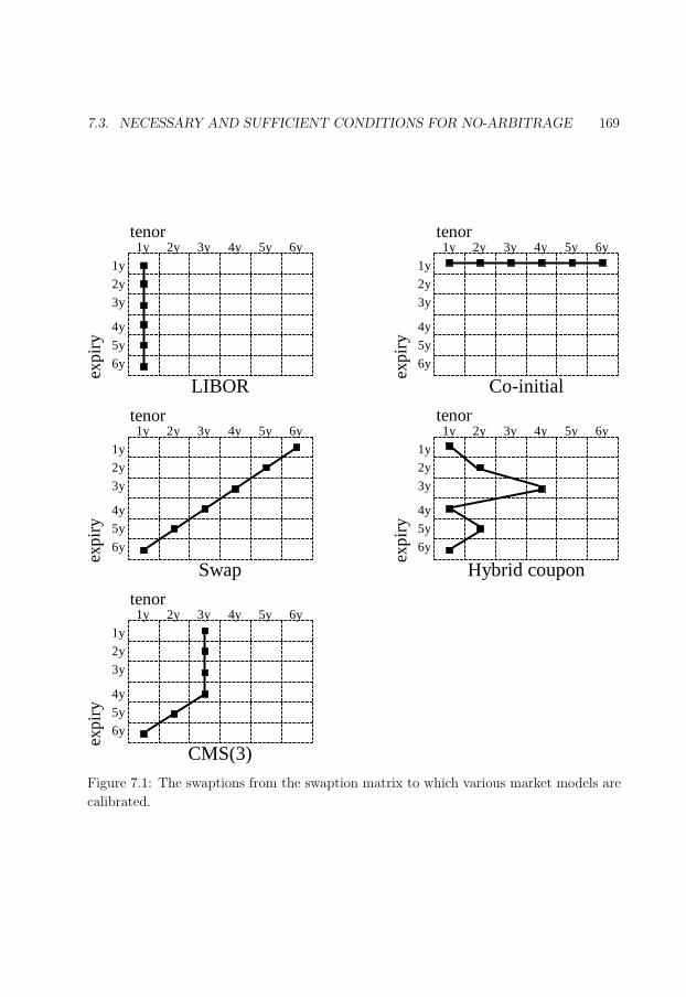
197

7.3. NECESSARY AND SUFFICIENT CONDITIONS FOR NO-ARBITRAGE 169

tenor1y 2y 3y 4y 5y 6y

1y

2y

3y

4y

5y

6y

expi

ry


1y

2y

3y

4y

5y

6y

expi

ry


1y

2y

3y

4y

5y

6y

expi

ry


1y

2y

3y

4y

5y

6y

expi

rytenor1y 2y 3y 4y 5y 6y

1y

2y

3y

4y

5y

6y

expi

ryLIBOR

Swap

CMS(3)

Co-initial

Hybrid coupon

Figure 7.1: The swaptions from the swaption matrix to which various market models are

calibrated.

198


t1y 2y 3y 4y 5y 6y

1

2

3

4

5

6

forw

ard

rate

inde

x

t1y 2y 3y 4y 5y 6y

1

2

3

4

5

6

forw

ard

rate

inde

x

t1y 2y 3y 4y 5y 6y

1

2

3

4

5

6

forw

ard

rate

inde

x

t1y 2y 3y 4y 5y 6y

1

2

3

4

5

6fo

rwar

d ra

te in

dex

t1y 2y 3y 4y 5y 6y

1

2

3

4

5

6

forw

ard

rate

inde

x

LIBOR

Swap

CMS(3)

Co-initial

Hybrid coupon

7y

7y

7y 7y

7y

Legendfixing datefixing and payment datepayment date

Figure 7.2: An overview of the forward swap agreements for various market models.

199


This equation can be seen to hold by considering a portfolio in the discount bonds that will

have the exact same cash flows as the floating leg, to wit, long a discount bond maturing

at time ts and short a bond maturing at time te. At time ts, we invest the proceeds of the

long position in the discount bond into the LIBOR deposit. At each LIBOR payment, we

re-invest the notional into the LIBOR deposit. At the end of the floating leg, the notional

cancels against the short position in the discount bond. It is not hard to see that such

procedure provides the exact same cash flows as a floating leg.

The value πfxd(ε, f) of a fixed leg with forward rate f can be obtained by simply

discounting back the known future cash flows4,

πfxd(ε, f) = f

e−1∑i=s

αibi+1

︸︷︷︸.

The under-braced expression is also called present value of a basis point (PVBP in short),

and is denoted by ps:e.

The conditions on the forward rates are governed by the forward swap agreements to

have zero value, that is, πflt(ε) − πfxd(ε, f) = 0. In fact, there exists a unique system of

prices for the discount bonds consistent with the forward rates if and only if the system

of m linear equations in the n unknown variables b2, . . . , bn+1 given by

bs(j) − be(j) −

e(j)−1∑

i=s(j)

fjαibi+1 = 0m

j=1, (7.3)

with b1 = 1, has a unique solution. The latter is already a precisely specified and tractable

necessary and sufficient condition for existence of unique discount bond prices that are

consistent with the forward rates. This condition can be validated by numerically check-

ing invertibility of linear equation (7.3). In the sequel, we will develop conditions and

implications that are more straightforward to verify and that a priori guarantee invert-

ibility of (7.3), and we will sketch scenarios in which these implications will hold. It will

be shown that invertibility of (7.3) is guaranteed in typical finance scenarios, and that

invertibility can be violated only under extreme situations, that are fully irrelevant to a

finance setting.

If m < n then if a solution exists, it is bound to exhibit non-uniqueness. If m > n,

then the system is in general over-determined. Only for a very particular choice of forward

rates fj, the system could then be degenerate, thereby still allowing for a unique solution.

Given arbitrarily specified forward rates however, the degeneracy will occur, if at all, only

occasionally. Generally specified forward rates span a non-degenerate set of equations,

4We assume, for notational simplicity only, that the fixed payment frequency equals the floatingpayment frequency.

200


thereby implying that, when m > n, in most cases the model does not have unique

discount bond prices. In other words, two different subsets of n forward rates determine,

via (7.3), two sets of discount bond prices that are different and thus inconsistent with

each other. The model should have the property that there exist unique discount bond

prices regardless of how the forward rates are specified. The possibility of degeneracy is

excluded by the following assumption on the values that the forward rates can attain.

Assumption 1 A forward rate f can only attain any non-negative value, that is, we

must have

f ≥ 0. (7.4)

Assumption 1 will be satisfied almost always in any interest rate market. Only in very

rare occasions have negative interest rates been observed. An example of negative in-

terest rates in Japan at the start of November 1998 is given in Ostrom (1998). These

interest rates reached -3 to -6 basis points (bp) (-.03% to -.06%). Moreover, the popular

displaced diffusion smile model of Rubinstein (1983) can generate negative forward rates

with positive probability, if the displacement parameter is negative. However, violation

of Assumption 1 does not necessarily imply that the system of forward rates admits ar-

bitrage of the weak form. In fact, we make plausible that slightly negative interest rates

still allow for unique discount bond prices that are arbitrage-free in the weak sense, by

considering a simple numerical example. We consider a single forward rate, two tenor

times t1 = 0, t2 market model. The price of the discount bond for maturity at time t2is given by 1/(1 + αf). The rate f should thus satisfy f > −1/α, to ensure a positive

and finite price for the discount bond. For annual payments, for which α ≈ 1, we have

−1/α ≈ −100%. In fact, for more frequent payments than annual, the arbitrage-defying

rate is even more negative than −100%. These considerations lead us to conclude that ar-

bitrage of the weak form in a forward swap agreement market can occur only in situations

that are considered financially extreme. Essential to no-arbitrage is thus the structure of

the forward swap agreements.

7.3.1 Main result

The main result can now be formulated. The theorem below states that, for dynamic

market models, (i) if a tenor structure has n fixing times t1, . . . , tn, then we require n

forward swap agreements, and (ii) for each fixing time ti, there is exactly one forward

swap agreement that starts at that fixing time ti, i = 1, . . . , n. We note that the co-initial

model does not fit the requirements below, though it is a perfectly sensible arbitrage-free

model. The reason that the co-initial model is not incorporated is the requirement that

a model be dynamic, see the discussion in Section 7.2.1.

201


Algorithm 4 Back substitution.

Input: n, U ((n + 1)× (n + 1) unit upper-triangular), c ∈ Rn+1.

Output: b = U−1c ∈ Rn+1.

1: Set bn+1 ⇐ cn+1.

2: for i = n, . . . , 1 do

3: bi ⇐ ci −∑n+1

j=i+1 uij bj.

4: end for

Theorem 8 Let t1, . . . , tn+1 be a set of tenor times. Let E = εjmj=1 and fj be a set of

forward swap agreements and forward rates, respectively, associated with the tenor times.

Then, at each of the times t1, . . . , tn, for all forward rates fjmj=1 satisfying Assumption

1, there exists a unique weak-form arbitrage-free solution to the system of linear equations

(7.3) in the discount bond prices, if and only if m = n and there exists an ordering of the

n forward swap agreements εj = (s(j), e(j)), j = 1, . . . , m such that s(j) = j.

PROOF: The proof is split into two parts. First, we prove that the described structure

of forward rates leads to arbitrage-free invertibility of system (7.3) for all forward rates

satisfying Assumption 1. Second, the reverse implication is proven.

Suppose that the structure E of forward swap agreements is such that m = n and

that there exists an ordering of the n forward swap agreements εj = (s(j), e(j)), j =

1, . . . , m such that s(j) = j. The existence of unique arbitrage-free discount bond prices

is guaranteed if we show there exists unique discount bond prices that are all positive.

To that order, consider system (7.3) in terms of the deflated discount bond prices, bi ≡bi/bn+1, and substitute s(j) = j,

bj − be(j) −

e(j)−1∑i=j

fjαibi+1 = 0

n

j=1

, bn+1 = 1. (7.5)

We note that the (n + 1) × (n + 1) matrix U = U(f) associated with this system is

unit upper-triangular, which means that the diagonal contains ones and that the lower-

triangular part of the matrix contains zeros. It follows that this matrix is invertible. We

thus have

U(f)b = c, b = U(f)−1c, c = (0 · · · 0 1)T ∈ Rn+1.

An efficient method for calculating the inverse of a unit upper-triangular matrix is back

substitution, see for example Golub & van Loan (1996, Algorithm 3.1.2). Back substitution

will aid in the proof, therefore it has been displayed in Algorithm 4. We show by induction

for i = n + 1, n, . . . , 1 that bi ≥ 1. For i = n + 1, bi = bn+1 = 1, by line 1 of Algorithm 4,

which states that bn+1 = cn+1 = 1. Suppose, then, that bj ≥ 1 for j = i + 1, . . . , n + 1.

202


We have, by line 3 of Algorithm 4, that bi = ci−∑n+1

j=i+1 uij bj = −∑n+1j=i+1 uij bj. We note

that, for j > i, uij is either −αjfi, −1− αjfi, or 0. It follows that

bi = fi

e(i)−1∑j=i

αj bj+1

︸︷︷︸≥0

+ be(i)︸︷︷︸≥1

≥ 1,

which concludes the induction proof. The unique solution for the undeflated discount

bond prices at tenor point t1 is then given by bi ≡ bi/b1, which is defined and positive

since b = (b1, . . . , bn+1) ≥ 1.

We note that the above proof is independent of the number of tenor times. Therefore

the forward swap agreements structure n = m and s(j) = j guarantees existence of

unique arbitrage-free discount bond prices for all forward rates satisfying Assumption 1

at all tenor times t1, . . . , tn, which was to be shown.

The reverse implication is proven by induction on n. For n = 1, the result is immediate.

Now, assume the result is true for i = 1 to n− 1. We want to prove it is true for n. The

model viewed from t2 has n tenor points, so by the induction hypothesis we must have

that: (i) m ≥ n−1, (ii) there are exactly n−1 forward swap agreements that start at t2 or

later, (iii) for these n− 1 forward swap agreements, there is an enumeration j = 2, . . . , n,

such that s(j) = j. There are three possibilities: m = n− 1, m > n or m = n. We show

that the cases m = n− 1 and m > n lead to non-uniqueness or non-invertibility of (7.3)

for some of the forward rates f that satisfy Assumption 1.

If m = n− 1, there are less equations than unknown variables in (7.3), and it follows

that, if there is a solution at all, it will be non-unique.

If m > n, then we may form a sub-model with n forward swap agreements such that

s(j) = j for j = 1, . . . , n. We have already proven that such a structure with n forward

rates leads to unique positive discount bond prices. For a left out forward swap agreement,

say ε = (s, e), the associated forward rate f should then satisfy

f =bs − be∑e−1i=s αibi+1

. (7.6)

We conclude then that there are forward rates satisfying Assumption 1 for which there

do not exist discount bond prices.

Thus we must have m = n and for remaining forward swap agreement 1 we have

s(1) = 1 from which the result follows. 2

As a corollary, we can count the dynamic market model structures given the number

of tenor times n + 1. For forward rate 1, we can chose from n end times t2, . . . , tn+1, for

forward rate 2, from n− 1 end times t3, . . . , tn+1, etcetera.

203

7.4. GENERIC EXPRESSIONS FOR NO-ARBITRAGE DRIFT TERMS 175

Corollary 2 (Counting dynamic market model structures) Consider market models with

n+1 tenor times. Then there are n! ways of selecting forward swap agreements such that,

for all forward rates satisfying Assumption 1, and at all tenor times t1, . . . , tn, there exist

unique weak-form arbitrage-free discount bond prices satisfying (7.3).

We note that Theorem 8 rules out the applicability of generic market models to

Bermudan-callable spread options, in the sense that we cannot define two rates, fixing at

the same time, as state variables.

7.4 Generic expressions for no-arbitrage drift terms

In this section, generic expressions are derived for the arbitrage-free drift terms of generic

market models, that are so characteristic for the LIBOR and swap market models. We

assume given a dynamic market model, therefore the forward swap agreements are of the

form εi = (i, e(i)). If dependency of the end index is clear we simply write e(i) as e. The

forward rate fi:e has start date ti and end date te. Forward rate fi:e is modelled under

its forward measure, which is associated with the p pi:e as numeraire. Forward rate fi:e is

modelled asdfi:e(t)

fi:e(t)= σi:e(t) · dw(i:e)(t), (7.7)

with σi:e denoting a d-dimensional volatility vector, and with w(i:e) a d-dimensional Brow-

nian motion under the forward measure Qi:e associated with pi:e as numeraire. The

positive integer d is deemed the number of factors of the model. The volatility vector

σi:e(t) = σi:e(t, ω) can be state dependent to allow for smile modelling.

For pricing of non-standard interest rate derivatives, it is necessary to jointly imple-

ment the above scheme (7.7) for all forward rates simultaneously. Therefore we must work

out the SDE for the forward rates under a single pricing measure. We can work either

with the terminal or spot measure. Each is treated below consecutively.

7.4.1 Terminal measure

In this subsection, we work with the terminal measureQn+1, that is the measure associated

with the terminal discount bond bn+1 as numeraire.

Without loss of generality, the presentation is given as if all forward rates have not yet

expired. We work with the numeraire-deflated discount bond prices. The quantity pi:e

denotes the deflated p, pi:e ≡ pi:e/bn+1. The deflated ps can be calculated, in turn, when

the deflated discount bond prices bi ≡ bi/bn+1 are known. The deflated discount bond

prices are given by (7.5). Recall that (7.5) can be written in matrix form as Ub = c, with

204


c = (0 · · · 0 1)T , and U = U(f) an (n + 1)× (n + 1) unit upper-triangular matrix, given

by

uij =

0 if i > j or (i < j and j > e(i)),

1 if i = j,

−αj−1fi:e(i) if i < j and j < e(i),

−αj−1fi:e(i) − 1 if i < j and j = e(i).

Thus b = U(f)−1c. We may write p as a function of the forward rates, p = p(f). In fact,

p = Ab, A ≡

0 (α1 · · · αe(1)−1 0 · · · 0)

0 0 (α2 · · · αe(2)−1 0 · · · 0)

0...

. . . . . ....

0 0 · · · 0 (αn)

,

for the n× (n + 1) matrix A. Thus, p = AU(f)−1c. Subsequently, we define the Radon-

Nikodym density

zi:e,n+1(t) ≡ pi:e(t)/bn+1(t)

pi:e(0)/bn+1(0)=

pi:e(t)

pi:e(0). (7.8)

We note that zi:e,n+1(t) is a martingale under the terminal measure Qn+1. This implies

thatdzi:e,n+1(t)

zi:e,n+1(t)=

dpi:e(t)

pi:e(t)= θi:e,n+1(t) ·w(n+1)(t), (7.9)

with the d-dimensional vector θ given by

θi:e,n+1(t) =1

pi:e(t)

n∑

k=i+1

∂pi:e

∂fk:e(k)

(t)fk:e(k)(t)σk:e(k)(t). (7.10)

The summation is required only from i + 1 to n since pi:e is dependent on fk:e(k) only

for k > i. Finally we apply Girsanov’s theorem to obtain the required expression for

dw(i:e)(t)− dw(n+1)(t),

dw(i:e)(t)− dw(n+1)(t) = −θi:e,n+1(t)dt. (7.11)

Thus,

dfi:e(t)

fi:e(t)= − 1

pi:e(t)

n∑

k=i+1

∂pi:e

∂fk:e(k)

(t)fk:e(k)(t)|σk:e(k)(t)||σi:e(t)|ρk:e(k),i:e(t)dt

+σi:e(t) · dw(n+1)(t),

where the scalar ρk:e(k),i:e has been defined as

ρk:e(k),i:e(t) =σk:e(k)(t) · σi:e(t)

|σk:e(k)(t)||σi:e(t)| ,

205

7.4. GENERIC EXPRESSIONS FOR NO-ARBITRAGE DRIFT TERMS 177

and has the interpretation of instantaneous correlation.

An expression is given for ∂p/∂fk:e(k). We note that ∂U/∂fk:e(k) is a matrix that is

zero bar a single row, the kth row, and that the derivative is independent of f , since all

f terms occur linearly in the matrix U. The kth row is filled, from entry (k, k + 1), with

the row vector (−αk · · · − αe(k)−1 0 · · · 0). We have that

∂p

∂fk:e(k)

= −AU−1 ∂U

∂fk:e(k)

U−1c = −AU−1 ∂U

∂fk:e(k)

b = AU−1ckpk:e(k), (7.12)

where ck ∈ Rn+1 denotes the standard basis vector with unit kth coordinate, and zero

coordinates otherwise. We define b(k)i by

b(k)i = (U−1ck)i, i = 1, . . . , n, k = 1, . . . , n. (7.13)

Substituting (7.13) into (7.12) yields

∂pi:e

∂fk:e(k)

= 1k≥i+1pk:e(k)

(min(e(i)−1,k−1)∑

j=i

αj b(k)j+1

). (7.14)

Define µ(i, k) ≡ min(e(i) − 1, k − 1). Substituting (7.14) into (7.12), suppressing the

dependency of time, and using pk:e(k)fk:e(k) = bk − be(k), we obtain the generic market

model SDE under the terminal measure:

dfi:e

fi:e

= − 1

pi:e

n∑

k=i+1

(bk − be(k)

)(

µ(i,k)∑j=i

αj b(k)j+1

)σk:e(k) · σi:edt + σi:e · dw(n+1). (7.15)

7.4.2 Spot measure

In this subsection, we work with the spot measure QSpot, that is the measure associated

with the spot LIBOR numeraire, defined as follows. The account starts out with one unit

of currency. Subsequently, this amount is invested in the spot LIBOR account. After the

first accrual period, the proceeds are re-invested in the then spot LIBOR account. This

procedure is repeated. For the spot measure it is convenient to define the spot index i(t),

defined by i(t) = mininteger i ; t < ti.For the spot measure, we work with discount bond prices, deflated by the spot discount

bond bi(t). The quantities p and b denote the vectors of bi(t)-deflated PVBPs and discount

bond prices, respectively. We have p = Ab and

b =1

bi(t)

b =1

(U−1c)i(t)

U−1c.

206


The Radon-Nikodym density zi:e,i(t)(t) is defined similarly to (7.8). A martingale SDE for

the Radon-Nikodym density holds,

dzi:e,i(t)(t)

zi:e,i(t)(t)=

dpi:e,i(t)(t)

pi:e,i(t)(t)= θi:e,i(t)(t) · dw(i(t)),

similar to (7.9), with d-dimensional volatility vector equal to

θi:e,i(t)(t) =1

pi:e(t)

n∑

k=i(t)

∂pi:e

∂fk:e(k)

(t)fk:e(k)(t)σk:e(k)(t). (7.16)

If we compare (7.16) to (7.10), we find that, for the spot measure, we sum over all available

forward rates from i(t) to n, since pi:e might depend on all those forward rates. Recall

that, for the terminal measure, we need only sum from i + 1 to n.

Similar to (7.11), we have dw(i:e)−dw(i(t)) = −θi:e,i(t)dt. Thus we obtain the equivalent

of (7.12),

dfi:e(t)

fi:e(t)= − 1

pi:e(t)

n∑

k=i(t)

∂pi:e

∂fk:e(k)

(t)fk:e(k)(t)|σk:e(k)(t)||σi:e(t)|ρk:e(k),i:e(t)dt

+σi:e(t) · dw(i(t))(t). (7.17)

An expression for ∂p/∂fk:e(k) is given by

∂p

∂fk:e(k)

=1

bi(t)

∂p

∂fk:e(k)

+1

bi(t)

(U−1 ∂U

∂fk:e(k)

U−1c

)

i(t)︸︷︷︸=pk:e(k)b

(k)i(t)

p. (7.18)

Similar as in (7.12) and (7.14) for the terminal measure, we find for the spot measure:

∂pi:e

∂fk:e(k)

= 1k≥i+1pk:e(k)

µ(i,k)∑j=i

αj b(k)j+1 − pk:e(k)pi:eb

(k)i(t). (7.19)

Substituting (7.19) into (7.17), suppressing the dependency of time, and using

pk:e(k)fk:e(k) = bk − be(k),

we obtain the generic market model SDE under the spot measure:

dfi:e

fi:e

= − 1

pi:e

n∑

k=i(t)

(bk − be(k)

)(

1k≥i+1

µ(i,k)∑j=i

αj b(k)j+1 − pi:eb

(k)i(t)

)σk:e(k)

·σi:edt + σi:e · dw(i(t)). (7.20)

207

7.5. COMPLEXITY 179

7.4.3 An example: The LIBOR market model

For illustration, in this section the LIBOR drift terms are calculated starting from the

generic market model framework. We stress here that the explicit calculation in this

section of the generic expressions of the previous section is not required for implementation

of the generic market model framework, but is merely performed for illustration only.

First, we derive the LIBOR SDE for the terminal measure, by applying (7.15). In the

LIBOR market model, a forward rate fk:e(k) is denoted by fk. We note that:

(i) pi:e(i) = pi:i+1 = αibi+1,

(ii) µ(i, k) = min(e(i)− 1, k − 1) = min(i, k − 1) = i, for k = i + 1, . . . , n,

(iii) b(k)j =

bj

bk1j≤k =

bj

bk1j≤k,

(iv) bk−bk+1

bk= bk−bk+1

bk= 1− 1

1+αkfk= αkfk

1+αkfk,

(v)∑µ(i,k)

j=i αj b(k)j+1 =

pi:e(i)

bk=

pi:e(i)

bk.

Substituting (i)–(v) into (7.15), we obtain,

dfi

fi

= −n∑

k=i+1

αkfk

1 + αkfk

σk · σidt + σi · dw(n+1),

which is the familiar expression for the SDE of the LIBOR market model under the

terminal measure.

Second, we derive the LIBOR SDE for the spot measure. If we substitute (i)–(v) into

(7.20), we see that for k ≥ i + 1,∑i

j=i αj b(k)j+1 cancels against pi:i+1b

(k)i(t), and for k ≤ i, we

are left with −pi:i+1b(k)i(t), therefore:

dfi

fi

=i∑

k=i(t)

αkfk

1 + αkfk

σk · σidt + σi · dw(i(t)),

which is the familiar expression for the SDE of the LIBOR market model under the spot

measure.

7.5 Complexity

We study the complexity of the drift calculation over a single time step in a numerical

implementation. For generic market models, we show that the complexity is, at worse,

of order O(n3). For specific market models, such as the LIBOR, swap, and CMS market

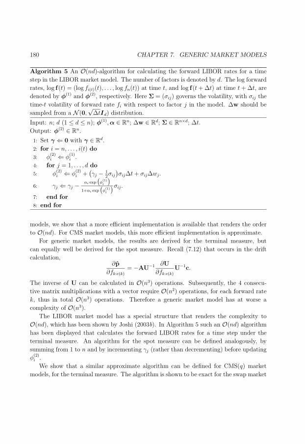
208


Algorithm 5 An O(nd)-algorithm for calculating the forward LIBOR rates for a time

step in the LIBOR market model. The number of factors is denoted by d. The log forward

rates, log f(t) = (log fi(t)(t), . . . , log fn(t)) at time t, and log f(t + ∆t) at time t + ∆t, are

denoted by φ(1) and φ(2), respectively. Here Σ = (σij) governs the volatility, with σij the

time-t volatility of forward rate fi with respect to factor j in the model. ∆w should be

sampled from a N (0,√

∆tId) distribution.

Input: n; d (1 ≤ d ≤ n); φ(1),α ∈ Rn; ∆w ∈ Rd; Σ ∈ Rn×d; ∆t.

Output: φ(2) ∈ Rn.

1: Set γ ⇐ 0 with γ ∈ Rd.

2: for i = n, . . . , i(t) do

3: φ(2)i ⇐ φ

(1)i .

4: for j = 1, . . . , d do

5: φ(2)i ⇐ φ

(2)i +

(γj − 1

2σij

)σij∆t + σij∆wj.

6: γj ⇐ γj − αi exp(

φ(1)i

)

1+αi exp(

φ(1)i

)σij.

7: end for

8: end for

models, we show that a more efficient implementation is available that renders the order

to O(nd). For CMS market models, this more efficient implementation is approximate.

For generic market models, the results are derived for the terminal measure, but

can equally well be derived for the spot measure. Recall (7.12) that occurs in the drift

calculation,∂p

∂fk:e(k)

= −AU−1 ∂U

∂fk:e(k)

U−1c.

The inverse of U can be calculated in O(n3) operations. Subsequently, the 4 consecu-

tive matrix multiplications with a vector require O(n2) operations, for each forward rate

k, thus in total O(n3) operations. Therefore a generic market model has at worse a

complexity of O(n3).

The LIBOR market model has a special structure that renders the complexity to

O(nd), which has been shown by Joshi (2003b). In Algorithm 5 such an O(nd) algorithm

has been displayed that calculates the forward LIBOR rates for a time step under the

terminal measure. An algorithm for the spot measure can be defined analogously, by

summing from 1 to n and by incrementing γj (rather than decrementing) before updating

φ(2)i .

We show that a similar approximate algorithm can be defined for CMS(q) market

models, for the terminal measure. The algorithm is shown to be exact for the swap market

209

7.5. COMPLEXITY 181

model (q = n). The following quantity that occurs in the drift term is approximated:

p(k)i:µ(i,k)+1 = p

(k)i:min(k,i+q) :=

min(k,i+q)−1∑j=i

αj b(k)j+1 (i < k). (7.21)

The approximation is based on the assumption that αi is close to αi+q, for i = 1, . . . , n−q.

We note that this assumption is used only to efficiently approximate (7.21) for calculation

of drift terms, and this assumption is not used in the calculation of contract payoffs.

Moreover, if needs be, the drift terms can be calculated exactly by exact calculation of

(7.21).

Approximation 1 Approximately, by assumption of αi ≈ αi+q (i = 1, . . . , n − q), we

have, for p(k)i:µ(i,k)+1 defined in (7.21),

p(k)i:µ(i,k)+1 ≈ αk−1

k−2∏m=i

(1 + αmfm+1:e(m+1)

)(i < k). (7.22)

Here, an empty product denotes 1. Formula (7.22) is exact for i > k−q−1. In particular,

(7.22) is exact for any i in the swap market model (q = n).

The rationale for Approximation 1, as well as the proof of exactness when i > k−q−1, are

given in Appendix 7.A. We note that accumulating errors in (7.22) are likely to cancel,

since in practice the difference αi − αi+q is both negative and positive. From (7.15) and

Approximation 1, we obtain,

dfi:e

fi:e

≈ − 1

pi:e

n∑

k=i+1

(bk − be(k)

)αk−1

k−2∏m=i

(1 + αmfm+1:e(m+1)

)σk:e(k) · σi:edt

+σi:e · dw(n+1). (7.23)

Define

vi =n∑

k=i+1

(bk − be(k)

)αk−1

k−2∏m=i

(1 + αmfm+1:e(m+1)

)σk:e(k). (7.24)

The proof of the following lemma has been deferred to Appendix 7.B.

Lemma 3 The quantity vi defined in (7.24) satisfies the following recursive formulas:

• vn = 0,

• vi =(1 + αifi+1:e(i+1)

)vi+1 + αi

(bi+1 − be(i+1)

)σi+1:e(i+1).

210


Algorithm 6 An O(nd)-algorithm for approximately calculating the forward swap rates

for a time step in the CMS(q) market model (exact when q = n), under the terminal

measure. The number of factors is denoted by d. The log forward rates, log f(t) =

(log fi(t):e(i(t))(t), . . . , log fn:e(n)(t)) at time t, and log f(t + ∆t) at time t + ∆t, are denoted

by φ(1) and φ(2), respectively. Here Σ = (σij) governs the volatility, with σij the time-t

volatility of forward rate fi:e(i) with respect to factor j. Here, e(·) is defined in (7.2). ∆w

should be sampled from a N (0,√

∆tId) distribution.

Input: n; d, q (1 ≤ d, q ≤ n); φ(1),α ∈ Rn; ∆w ∈ Rd; Σ ∈ Rn×d; ∆t.

Output: φ(2) ∈ Rn.

1: βn+1 ⇐ 1. $n+1 ⇐ 0.

2: for i = n, . . . , i(t) do

3: $i ⇐ $i+1 + αiβi+1 − 1i<n & e(i)=e(i+1)−1αe(i+1)−1βe(i+1).

4: f(1)i ⇐ exp(φ

(1)i ).

5: βi ⇐ $if(1)i + βe(i).

6: If i = n, set vn ⇐ 0 ∈ Rd, else (i < n), set

vi ⇐(1 + αif

(1)i+1

)vi+1 + αi

(βi+1 − βe(i+1)

)σi+1.

7: φ(2)i ⇐ φ

(1)i +

(− 1

$ivi − 1

2σi

)· σi∆t + σi ·∆w.

8: end for

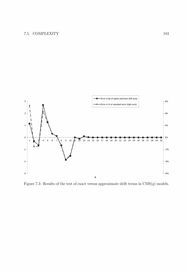
211

7.5. COMPLEXITY 183

-3

-2

-1

0

1

2

3

1 2 3 4 5 6 7 8 9 10 11 12 13 14 15 16 17 18 19 20 21 22 23 24 25 26 27 28 29 30

q

-6%

-4%

-2%

0%

2%

4%

6%Error in bp of option premium (left axis)

Error in % of standard error (right axis)

Figure 7.3: Results of the test of exact versus approximate drift terms in CMS(q) models.

212


Table 7.2: Deal description for the test of exact versus approximate drift terms in CMS(q)

models.

Currency: USD

Market data: Swap rates and at-the-money swaption volatility

Valuation date: 18 July 2003

Deal: 30 year fixed-maturity Bermudan swaption

Start date: 16 June 2004

Frequency: Annual

Day count: ACT/365

Date roll: Modified following

Fixed coupon: 3.2%

In Algorithm 6 an O(nd) algorithm, based on Lemma 3, is displayed that approximately

calculates the forward swap rates for a time step under the terminal measure, for the

CMS(q) market model. This algorithm is exact for the swap market model (q = n).

Algorithm 6 also calculates time-t values for discount bond prices (denoted by β) and for

PVBPs (pi:e(i) is denoted by $i).

To benchmark the accuracy of Algorithm 6, various fixed-maturity Bermudan swap-

tions are priced in their corresponding CMS(q) market models, with both exact SDE

(7.15) and approximate SDE (7.23). The deal specification is given in Table 7.2. The

swap tenor is q years, with 31 − q exercise opportunities, at (16 June 2004 + i years),

i = 0, . . . , 30 − q, for q = 1, . . . , 30. The difference between the minimum (0.996) and

maximum (1.007) attained day count fractions is 0.011. To price fixed-maturity Bermu-

dan swaptions in Monte Carlo, we use the algorithm of Longstaff & Schwartz (2001), with

the swap value as explanatory variable x, and basis functions 1, x and x2. An 8 factor

model is used (d = 8), with the correlation of the forward CMS(q) rates given by the

parametrization of Rebonato (1998, Equation (4.5), page 83), exp(−β|ti − tj|), for rates

fi:e(i) and fj:e(j), with β = 3%. The differences between the prices obtained with exact

and approximate drift terms are displayed in Figure 7.3. We note that for q = n, equal

prices are obtained up to all digits. The results show that the error is small, up to only 3

bp of the option premium, and up to only 6% of the simulation standard error. Moreover,

the error fluctuates robustly around 0, since the difference αi−αi+q is both negative and

positive, in practice.

A significant reduction of computational time can thus be attained by selecting a low

number of factors d. A result of using a low number of factors is that the instantaneous

correlation matrix (ρij) cannot be exactly fit to the historically estimated or market

213

7.6. GENERIC CALIBRATION TO CORRELATION 185

implied correlation matrix. The procedure for fitting a generic market model to correlation

is exactly the same as for the LIBOR market model. For fitting a low-factor LIBOR

market model to correlation, the reader is referred to Pietersz & Groenen (2004a, b) (see

Chapter 3), Grubisic & Pietersz (2005) (see Chapter 4), Wu (2003) and Rebonato (2002,

Section 9) or Brigo (2002).

7.6 Generic calibration to correlation

When each particular interest rate derivative has its own generic market model that is

used for its valuation and risk management, then the associated input correlation to those

models involves different interest rates. There is a relationship between these correlations,

and this relationship allows for netting correlation risk or reserves. Moreover, utilizing the

relationship between the correlations means that correlation is determined consistently

across different products. In general all interest rate correlations stem from the correla-

tions between different segments of the yield curve. In this section we show how forward

LIBOR correlations can be used to determine subsequently the correlations for any of the

generic market models specific to certain interest rate products.

The advantage of considering all correlations in this way comes from the fact that

one can treat correlation risk (or reserves) in a consistent fashion across all interest rate

products. Netting of correlation reserves will subsequently occur naturally. Furthermore

only instantaneous forward LIBOR correlations have to be determined and administered.

The key to the method is the well-known fact that, within the LIBOR market model,

the instantaneous volatility vector σs:e(t) of a forward swap rate fs:e can be expressed as

weighted averages of instantaneous volatility vectors σi(t) of forward LIBORs,

σs:e(t) =e−1∑i=s

ws:ei (t)σi(t).

An expression for the weights ws:ei may be found, for example, in Hull & White (2000, page

53). The weights ws:ei are state dependent. A highly accurate deterministic approximation

σs:e(t) for the instantaneous volatility can however be obtained by evaluating the weights

at time zero,

σs:e(t) =e−1∑i=s

ws:ei (0)σi(t).

From the preceding considerations it should be clear that the instantaneous forward rate

correlation ρs(1):e(1),s(2):e(2)(t) can be approximately expressed as a function of the instan-

214


taneous forward LIBOR correlations ρij(t),

ρs(1):e(1),s(2):e(2)(t) = ρ

(dfs(1):e(1)(t)

fs(1):e(1)(t),dfs(2):e(2)(t)

fs(2):e(2)(t)

)

=σT

s(1):e(1)(t)σs(2):e(2)(t)√σT

s(1):e(1)(t)σs(1):e(1)(t)σTs(2):e(2)(t)σs(2):e(2)(t)

,

where

σTi:j(t)σk:l(t) ≈ σT

i:j(t)σk:l(t)

=

j−1∑m1=i

l−1∑

m2=k

wi:jm1

(0)wk:lm2

(0)|σm1(t)||σm2(t)|ρm1m2(t).

7.7 Conclusions

In this chapter, a generalization of market models has been studied, whereby arbitrary

forward rates are allowed to span the tenor structure relevant to an interest rate derivative.

The benefit of such generalization is that straightforward volatility-calibration can be

achieved for the fixings of LIBOR or swap rates relevant to the interest rate derivative.

Generic market models are therefore particularly apt for pricing and risk management of

CMS and hybrid coupon swaps, and callable and cancellable versions thereof, in particular,

Bermudan CMS swaptions and fixed-maturity Bermudan swaptions. We showed that the

LIBOR and swap market models are special cases of the generic market model framework.

The need for a generic specification of market models has been illustrated by counting

the admissible market model structures with n + 1 tenor times. We found n! possible

market models. For example, already only for an annual-paying deal of 10 years, there

are 10!=3,628,800 market models, thereby establishing the need for a generic specification.

Necessary and sufficient conditions were derived for a set of forward swap agreements to

provide a unique solution for discount bond prices, essentially regardless of the scenario

of attained forward rates. The major novelty of this chapter is the derivation of generic

expressions for no-arbitrage drift terms in generic market models. We developed a novel

algorithm of order O(nd) for approximate drift calculations in CMS market models under

the terminal measure.

7.A Appendix: Rationale for Approximation 1

We proceed by induction on i = k − 1, . . . , i(t).

• For i = k − 1: p(k)i:µ(i,k)+1 = p

(k)k−1:min(k,k−1+q) = αk−1b

(k)k = αk−1.

215

7.B. APPENDIX: PROOF OF LEMMA 3 187

• For i = k − 2, . . . , k − q, we have min(k, i + q) = k. The quantity b(k)i+1 satisfies:

b(k)i+1 = fi+1:e(i+1)p

(k)i+1:k. (7.25)

To see this, note that from line 3 of Algorithm 4, we have:

b(k)i+1 = fi+1:e(i+1)p

(k)i+1:i+q+1 + b

(k)i+q+1. (7.26)

From the definition b(k)j = (U−1ck)j in (7.13), we deduce that b

(k)j = 0 for j > k,

from which (7.25) follows. We obtain:

p(k)i:k = p

(k)i:k = p

(k)i+1:k + αib

(k)i+1 = p

(k)i+1:k

(1 + αifi+1:e(i+1)

)

(∗)= αk−1

k−2∏m=i+1

(1 + αmfm+1:e(m+1)

)(1 + αifi+1:e(i+1)

)

= αk−1

k−2∏m=i

(1 + αmfm+1:e(m+1)

),

where equality (∗) follows from the induction hypothesis.

• For i = k − q − 1, . . . , i(t), we have min(k, i + q) = i + q. From (7.26), we deduce:

p(k)i:µ(i,k)+1 = p

(k)i:i+q = αib

(k)i+1 − αi+q b

(k)i+q+1 + p

(k)i+1:i+q+1

= αi

(fi+1:e(i+1)p

(k)i+1:i+q+1 + b

(k)i+q+1

)− αi+q b

(k)i+q+1 + p

(k)i+1:i+q+1

(∗)≈ p(k)i+1:i+q+1

(1 + αifi+1:e(i+1)

)

= αk−1

k−2∏m=i

(1 + αmfm+1:e(m+1)

),

where in approximation (∗), we have used αi ≈ αi+q. 2

7.B Appendix: Proof of Lemma 3

For i < n,

vi =n∑

k=i+1

(bk − be(k)

)αk−1

k−2∏m=i

(1 + αmfm+1:e(m+1)

)σk:e(k)

=(bi+1 − be(i+1)

)αiσi+1:e(i+1) +

(1 + αifi+1:e(i+1)

)×

n∑

k=i+2

(bk − be(k)

)αk−1

k−2∏m=i+1

(1 + αmfm+1:e(m+1)

)σk:e(k)

=(1 + αifi+1:e(i+1)

)vi+1 + αi

(bi+1 − be(i+1)

)σi+1:e(i+1),

216


which was to be shown. 2

217

Chapter 8

Conclusions

In this thesis, innovations on efficient pricing and risk-management of Bermudan-style

interest rate derivatives are presented. The main pricing model for these derivatives is

the LIBOR market model (see Brace et al. (1997), Jamshidian (1997) and Miltersen et

al. (1997)). It allows for efficient calibration to volatility and correlation.

The most outstanding result of the thesis is the development of new market models,

named CMS and generic market models (Chapter 7). We specify precisely when an

arbitrary structure of forward rates is arbitrage-free at all possible (future) states of

the model. Via matrix notation, we are able to transform CMS and generic pricing

measures to spot and terminal measures, which enables a Monte Carlo implementation

of the models. Moreover, we present an efficient algorithm to accurately approximate

forward CMS rates over time steps during simulation in CMS market models. CMS and

generic market models allow for efficient volatility calibration (i.e., the model parameter

is the market implied volatility) of a whole new class of derivatives, such as fixed-maturity

Bermudan swaptions and Bermudan CMS swaptions.

A breakthrough on pricing callable products (e.g., Bermudan swaptions) in market

models can be found in Chapter 6. There, the least-squares Monte Carlo (MC) algorithm

of Longstaff & Schwartz (2001) is studied for estimating the optimal exercise decision for

American options with MC. A discontinuity occurs in the least-squares MC algorithm,

whereby finite difference estimates of risk sensitivities are inefficient. We propose a mod-

ification of the least-squares MC algorithm, named constant exercise decision method.

Hedge tests with Bermudan swaptions on USD data show that reduction of variance of

profit and loss (P&L) is much greater and acceptable when the constant exercise decision

method is used.

Chapter 6 contains many more results: First, hedge tests show that jointly delta

and vega hedging outperforms delta hedging only. Second, tests show that correlation

pricing impact on Bermudan swaptions is significant. It is shown that correlation can

be accurately captured in both single-factor models (e.g., the Markov-functional model of

218

190 CHAPTER 8. CONCLUSIONS

Hunt et al. (2000)) and multi-factor models (e.g., market models). Third, hedge tests show

that the following do not significantly impact reduction of variance of P&L: correlation,

number of factors, or, use of multi-factor models versus single-factor models. Fourth,

tests show that the pricing impact of volatility smile can be much larger than the pricing

impact of correlation.

As stated above, correlation still remains an important aspect of pricing derivatives,

even though correlation impact on hedging is small and smile is more important (for

the empirical findings in Chapter 6). Full-factor market models allow for straightforward

calibration to correlation, in the sense that the model parameter is literally the real-

world observed correlation value. For low-factor market models however, the situation is

different. Here, any model attainable correlation matrix has a rank equal to the number of

factors in the model, and this rank restriction usually does not hold for the given real-world

correlation matrix. Therefore, we need to find the low-rank correlation matrix closest to

the given matrix. This optimization problem is non-convex, and therefore hard to solve.

The process of finding the nearest low-rank correlation matrix is called rank reduction

of the correlation matrix. This thesis includes some of the forefront knowledge on this

topic, via Chapters 3 and 4. Two completely different solution algorithms are presented,

based on majorization and geometric programming. In extensive numerical tests, these

two algorithms seem to outperform existing algorithms, in terms of computational speed.

Both methods enjoy global convergence properties. Geometric Newton has a quadratic

rate of convergence, and geometric conjugate gradient has m-steps quadratic convergence,

where m is the dimension of the manifold. Moreover, we develop a method to instantly

check whether a stationary point (i.e., a point with negligible gradient) is in fact a global

minimum, which is quite an uncommon feature for a non-convex programming problem.

A discretization can be thought of as a translation of a continuous-time model to a

numerical algorithm aimed to implement the model. For the LIBOR market model, a new

and so-called Brownian bridge discretization is introduced in Chapter 5. The Brownian

bridge is specifically designed for single or large time steps. For single time steps, Brownian

bridge is least-squares optimal over all other discretizations (in a certain sense). This

is confirmed in an extended version of the numerical LIBOR-in-arrears test of Hunter

et al. (2001). Viewed as a multi step scheme, theoretical results show that Brownian

bridge converges weakly with order one. Moreover, we show that a mild assumption on

volatility, named separability, in combination with a single time step scheme, yields much

more efficient pricing on a grid or recombining lattice, instead of Monte Carlo simulation.

An important result is given in Chapter 2. Empirical tests highlight the effect of

various popular calibration choices on the quality of risk sensitivity estimates of Bermudan

swaptions priced with the LIBOR market model. So-called time-homogeneous choices lead

to poor and unstable estimates of risk, whereas the so-called constant volatility choice leads

to stable and efficient estimates. The results are important to practitioners that need to

219

191

choose a calibration method for market models, with the aim to risk manage Bermudan

swaptions and other interest rate derivatives.

220

221

Nederlandse samenvatting

(Summary in Dutch)

Waarderingsmodellen voor Bermuda-stijl rente derivaten

Bermuda-stijl rente derivaten vormen een belangrijke klasse van opties. Veel bancaire en

verzekeringsproducten, zoals hypotheken, vervroegd aflosbare obligaties, en levensverzek-

eringen, bevatten Bermuda rente opties, die een gevolg zijn van de mogelijkheid tot

vervroegde terugbetaling of stopzetting van het contract. Het veel voorkomen van deze

opties maakt duidelijk dat het belangrijk is, voor banken en verzekeraars, om de waarde

en risico van deze producten op de juiste manier in te schatten. Het juist inschatten

van het risico maakt het mogelijk om markt risico af te dekken met onderliggende en

regelmatig verhandelde waardes en opties. Waarderingsmodellen moeten arbitrage-vrij

zijn, en dienen consistent te zijn met (gekalibreerd te zijn aan) prijzen van actief ver-

handelde onderliggende opties. De dynamica van de modellen moet overeen komen

met de geobserveerde dynamica van de rente-termijnstructuur, zoals bijvoorbeeld cor-

relatie tussen rentestanden. Bovendien moeten waarderingsalgoritmes efficient zijn: Fi-

nanciele beslissingen gebaseerd op derivaten waarderingsberekeningen worden veeleer bin-

nen enkele seconden genomen, dan binnen uren of dagen. In recente jaren is een succesvolle

klasse van modellen naar voren gekomen, genaamd markt modellen. Dit proefschrift, on-

der begeleiding van Antoon Pelsser en Ton Vorst, breidt de theorie van markt modellen

uit, door: (i) een nieuwe, efficiente en meer nauwkeurige benaderende waarderingstech-

niek te introduceren, (ii) twee nieuwe en snelle algoritmes voor correlatie-kalibratie te

presenteren, (iii) nieuwe modellen te ontwikkelen die een efficiente kalibratie toestaan

voor een hele nieuwe klasse van derivaten, zoals vaste-looptijd Bermuda rente opties, en

(iv) nieuwe empirische vergelijkingen te presenteren van bestaande kalibratie technieken

en modellen, in termen van reductie van risico.

222

223

Bibliography

Abraham, R., Marsden, J. E. & Ratiu, T. (1988), Manifolds, Tensor Analysis, and Ap-

plications, Springer-Verlag, Berlin.

Al-Baali, M. (1985), ‘Descent property and global convergence of the Fletcher-Reeves

method with inexact line search’, IMA Journal of Numerical Analysis 5, 121–124.

Andersen, L. & Andreasen, J. (2000), ‘Volatility skews and extensions of the LIBOR

market model’, Applied Mathematical Finance 7(1), 1–32.

Andersen, L. & Andreasen, J. (2001), ‘Factor dependence of bermudan swaptions: fact

or fiction?’, Journal of Financial Economics 62(1), 3–37.

Apostol, T. M. (1967), Calculus, Vol. 1, 2 edn, John Wiley & Sons, Chichester.

Avellaneda, M. & Gamba, R. (2001), Conquering the Greeks in Monte Carlo: Efficient

calculation of the market sensitivities and hedge-ratios of financial assets by direct

numerical simulation, in ‘Proceedings of the First Bachelier Congress’, Paris.

Avellaneda, M., Holmes, R., Friedman, C. & Samperi, D. (1997), ‘Calibration of volatility

surfaces via relative-entropy minimization’, Applied Mathematical Finance 4(1), 37–

64.

Avramidis, A. N. & Matzinger, H. (2004), ‘Convergence of the stochastic mesh estimator

for pricing Bermudan options’, Journal of Computational Finance 7(4), 73–91.

Baxter, M. W. & Rennie, A. J. O. (1996), Financial calculus: An introduction to derivative

pricing, Cambridge University Press, Cambridge.

Bennett, M. N. & Kennedy, J. E. (2004), A comparison of Markov-functional

and market models: The one-dimensional case, www2.warwick.ac.uk/fac/sci/

statistics/staff/research students/mbennett/.

Berridge, S. & Schumacher, J. M. (2003), ‘An irregular grid method for high-

dimensional free-boundary problems in finance’, Future Generation Computer Sys-

tems 20(3), 353–362.

224

196 BIBLIOGRAPHY

Bjork, T. (2004), Arbitrage Theory in Continuous Time, 2 edn, Oxford University Press,

Oxford.

Bjork, T., Landen, C. & Svensson, L. (2004), ‘Finite-dimensional Markovian realiza-

tions for stochastic volatility forward-rate models’, Proceedings of the Royal Society

460(2041), 53–83. Series A.

Black, F. (1976), ‘The pricing of commodity contracts’, Journal of Financial Economics

3(2), 167–179.

Black, F. & Karasinski, P. (1991), ‘Bond and option pricing when short rates are lognor-

mal’, Financial Analysts Journal 47(4), 52–59.

Black, F. & Scholes, M. (1973), ‘The pricing of options corporate liabilities’, Journal of

Political Economy 81(3), 637–654.

Black, F., Derman, E. & Toy, W. (1990), ‘A one-factor model of interest rates and its

applications to treasury and bond options’, Financial Analysts Journal 46(1), 33–39.

Borg, I. & Groenen, P. J. F. (1997), Modern Multidimensional Scaling, Springer-Verlag,

Berlin.

Brace, A. & Womersley, R. S. (2000), Exact fit to the swaption volatility matrix using

semidefinite programming, presented at the ICBI Global Derivatives Conference,

Paris.

Brace, A., Dun, T. & Barton, G. (1998), Towards a central interest rate model, presented

at the ICBI Global Derivatives Conference, Paris.

Brace, A., Gatarek, D. & Musiela, M. (1997), ‘The market model of interest rate dynam-

ics’, Mathematical Finance 7(2), 127–155.

Brennan, M. J. & Schwartz, E. S. (1979), ‘A continuous time approach to the pricing of

bonds’, Journal of Banking and Finance 3(2), 133–155.

Brigo, D. (2002), A note on correlation and rank reduction, www.damianobrigo.it.

Brigo, D. & Mercurio, F. (2001), Interest Rate Models: Theory and Practice, Springer-

Verlag, Berlin.

Broadie, M. & Glasserman, P. (1996), ‘Estimating security price derivatives using simu-

lation’, Management Science 42(2), 269–285.

Broadie, M. & Glasserman, P. (2004), ‘A stochastic mesh method for pricing high-

dimensional American options’, Journal of Computational Finance 7(4), 35–72.

225

BIBLIOGRAPHY 197

Cairns, A. J. G. (2004), Interest Rate Models: An Introduction, Princeton University

Press, New Jersey.

Choy, B., Dun, T. & Schlogl, E. (2004), ‘Correlating market models’, Risk Magazine

pp. 124–129. September.

Chu, M. T., Funderlic, R. E. & Plemmons, R. J. (2003), ‘Structured low rank approxi-

mation’, Linear Algebra and its Applications 366, 157–172.

Cox, J. C. & Ross, S. A. (1976), ‘The valuation of options for alternative stochastic

processes’, Journal of Financial Economics 3(2), 145–166.

Cox, J. C., Ingersoll, J. E. & Ross, S. A. (1985), ‘A theory of the term structure of interest

rates’, Econometrica 53(2), 385–408.

Dai, Q. & Singleton, K. (2003), ‘Term structure dynamics in theory and reality’, Review

of Financial Studies 16(3), 631–678.

D’Aspremont, A. (2002), Calibration and Risk-Management Methods for the Libor Mar-

ket Model Using Semidefinite Programming, PhD thesis, Ecole Polytechnique, Paris.

D’Aspremont, A. (2003), ‘Interest rate model calibration using semidefinite programming’,

Applied Mathematical Finance 10(3), 183–213.

Davies, P. I. & Higham, N. J. (2000), ‘Numerically stable generation of correlation ma-

trices and their factors’, BIT 40, 640–651.

De Jong, F., Driessen, J. & Pelsser, A. A. J. (2004), ‘On the information in the interest

rate term structure and option prices’, Review of Derivatives Research 7(2), 99–127.

De Leeuw, J. & Heiser, W. J. (1977), Convergence of correction-matrix algorithms for

multidimensional scaling, in J. C. Lingoes, E. E. Roskam & I. Borg, eds, ‘Geometric

representations of relational data’, Mathesis Press, Ann Arbor, MI, pp. 735–752.

Dedieu, J.-P., Priouret, P. & Malajovich, G. (2003), ‘Newton’s method on Riemannian

manifolds: Covariant alpha-theory’, IMA Journal of Numerical Analysis 23(3), 395–

419.

Depczynski, U. & Stockler, J. (1998), A differential geometric approach to equidistributed

knots on Riemannian manifolds, in C. K. Chui & L. L. Schumaker, eds, ‘Approxima-

tion Theory IX, Theoretical Aspects’, Vol. 1, Vanderbilt University Press, Nashville,

TN, pp. 99–106.

do Carmo, M. P. (1992), Riemannian Geometry, 12 edn, Birkhauser, Boston, MA.

226

198 BIBLIOGRAPHY

Dolan, E. D. & More, J. J. (2002), ‘Benchmarking optimization software with performance

profiles’, Mathematical Programming, Series A 91(2), 201–213.

Dothan, L. U. (1978), ‘On the term structure of interest rates’, Journal of Financial

Economics 6(1), 59–69.

Driessen, J., Klaassen, P. & Melenberg, B. (2003), ‘The performance of multi-factor term

structure model for pricing and hedging caps and swaptions’, Journal of Financial

abd Quantitative Analysis 38(3), 635–672.

Duistermaat, J. J. & Kolk, J. A. C. (2000), Lie Groups, Springer-Verlag, Berlin.

Dykstra, R. L. (1983), ‘An algorithm for restricted least squares regression’, Journal of

the American Statistical Association 87(384), 837–842.

Edelman, A. & Lippert, R. (2000), Nonlinear eigenvalue problems with orthogonality

constraints (section 8.3), in Z. Bai, J. Demmel, J. Dongarra, A. Ruhe & H. van der

Vorst, eds, ‘Templates for the Solution of Algebraic Eigenvalue Problems: A Practical

Guide’, SIAM, Philidelphia.

Edelman, A., Arias, T. A. & Smith, S. T. (1999), ‘The geometry of algorithms with

orthogonality constraints’, SIAM Journal of Matrix Analysis and its Applications

20(2), 303–353.

Fan, R., Gupta, A. & Ritchken, P. (2003), ‘Hedging in the possible presence of un-

spanned stochastic volatility: Evidence from swaption markets’, Journal of Finance

58(5), 2219–2248.

Fletcher, R. & Reeves, C. M. (1964), ‘Function minimization by conjugate gradients’,

Computer Journal 7(2), 149–154.

Flury, B. (1988), Common Principal Components and Related Multivariate Models, J.

Wiley & Sons, New York.

Fournie, E., Lasry, J.-M., Lebuchoux, J., Lions, P.-L. & Touzi, N. (1999), ‘Applications

of Malliavin calculus to Monte Carlo methods in finance’, Finance and Stochastics

3(4), 391–412.

Galluccio, S. & Hunter, C. J. (2004), ‘The co-initial swap market model’, Economic Notes

33(2), 209–232.

Galluccio, S., Huang, Z., Ly, J.-M. & Scaillet, O. (2004), Theory and calibration of swap

market models, Working Paper, June Version.

227

BIBLIOGRAPHY 199

Gilbert, J.-C. & Nocedal, J. (1992), ‘Global convergence properties of conjugate gradient

methods for optimization’, SIAM Journal on Optimization 2(1), 21–42.

Glasserman, P. (2004), Monte Carlo Methods in Financial Engineering, Springer-Verlag,

Berlin.

Glasserman, P. & Merener, N. (2003a), ‘Cap and swaption approximations in LIBOR

market models with jumps’, Journal of Computational Finance 7(1), 1–36.

Glasserman, P. & Merener, N. (2003b), ‘Numerical solution of jump-diffusion LIBOR

market models’, Finance and Stochastics 7(1), 1–27.

Glasserman, P. & Merener, N. (2004), ‘Convergence of a discretization scheme for jump-

diffusion processes with state-dependent intensities’, Proceedings of the Royal Society

460(2041), 111–127. Series A.

Glasserman, P. & Zhao, X. (1999), ‘Fast Greeks by simulation in forward LIBOR models’,

Journal of Computational Finance 3(1), 5–39.

Glasserman, P. & Zhao, X. (2000), ‘Arbitrage-free discretization of lognormal forward

LIBOR and swap rate models’, Finance and Stochastics 4(1), 35–68.

Glunt, W., Hayden, T. L., Hong, S. & Wells, J. (1990), ‘An alternating projection algo-

rithm for computing the nearest Euclidean distance matrix’, SIAM Journal of Matrix

Analysis and its Applications 11(4), 589–600.

Golub, G. H. & van Loan, C. F. (1996), Matrix Computations, 3 edn, John Hopkins

University Press, Baltimore, MD.

Grubisic, I. (2002), Interest rate theory: BGM model, Master’s thesis, Mathematical

Institute, Leiden University. www.math.uu.nl/people/grubisic.

Grubisic, I. & Pietersz, R. (2005), Efficient rank reduction of correlation matrices,

www.few.eur.nl/few/people/pietersz.

Han, S.-P. (1988), ‘A successive projection method’, Mathematical Programming 40, 1–14.

Hayden, T. L. & Wells, J. (1988), ‘Approximation by matrices positive semidefinite on a

subspace’, Linear Algebra and its Applications 109, 115–130.

Heath, D., Jarrow, R. & Morton, A. (1992), ‘Bond pricing and the term structure of

interest rates: A new methodology for contingent claims valuation’, Econometrica

60(1), 77–105.

228

200 BIBLIOGRAPHY

Heiser, W. J. (1995), Convergent computation by iterative majorization: Theory and

applications in multidimensional data analysis, in W. J. Krzanowski, ed., ‘Recent

Advances in Descriptive Multivariate Analysis’, Oxford University Press, Oxford,

pp. 157–189.

Higham, N. J. (2002), ‘Computing the nearest correlation matrix–a problem from finance’,

IMA Journal of Numerical Analysis 22(3), 329–343.

Ho, T. S. Y. & Lee, S.-B. (1986), ‘Term structure movements and pricing interest rate

contingent claims’, Journal of Finance 41(5), 1011–1029.

Horn, R. A. & Johnson, C. R. (1990), Matrix Analysis, Cambridge University Press,

Cambridge.

Hughston, L. P. & Rafailidis, A. (2005), ‘A chaotic approach to interest rate modelling’,

Finance and Stochastics 9(1), 43–65.

Hull, J. C. (2000), Options, Futures, and Other Derivatives, 4 edn, Prentice-Hall, London.

Hull, J. C. & White, A. (1990), ‘Pricing interest-rate-derivative securities’, Review of

Financial Studies 3(4), 573–592.

Hull, J. C. & White, A. (2000), ‘Forward rate volatilities, swap rate volatilities, and

implementation of the LIBOR market model’, Journal of Fixed Income 10(2), 46–

62.

Hunt, P. & Kennedy, J. E. (2000), Financial Derivatives in Theory and Practice, John

Wiley & Sons, Chichester.

Hunt, P., Kennedy, J. E. & Pelsser, A. A. J. (2000), ‘Markov-functional interest rate

models’, Finance and Stochastics 4(4), 391–408.

Hunter, C. J., Jackel, P. & Joshi, M. S. (2001), ‘Getting the drift’, Risk Magazine. July.

Jackel, P. (2002), Monte Carlo Methods in Finance, J. Wiley & Sons, Chichester.

Jackel, P. & Rebonato, R. (2003), ‘The link between caplet and swaption volatilities in a

Brace-Gatarek-Musiela/Jamshidian framework: approximate solutions and empirical

evidence’, Journal of Computational Finance 6(4), 41–59.

Jamshidian, F. (1989), ‘An exact bond option formula’, Journal of Finance 44(1), 205–

209.

Jamshidian, F. (1997), ‘LIBOR and swap market models and measures’, Finance and

Stochastics 1(4), 293–330.

229

BIBLIOGRAPHY 201

Jamshidian, F. (2003), Minimax optimality of Bermudan and American claims and their

Monte-Carlo upper bound approximation, NIB Capital Bank, working paper.

Joshi, M. S. (2003a), The Concepts and Practice of Mathematical Finance, Cambridge

University Press, Cambridge.

Joshi, M. S. (2003b), ‘Rapid computation of drifts in a reduced factor LIBOR market

model’, Wilmott Magazine 5, 84–85.

Joshi, M. S. & Theis, J. (2002), ‘Bounding Bermudan swaptions in a swap-rate market

model’, Quantitative Finance 2(5), 370–377.

Karatzas, I. & Shreve, S. E. (1991), Brownian Motion and Stochastic Calculus, 2 edn,

Springer-Verlag, Berlin.

Kerkhof, J. & Pelsser, A. A. J. (2002), ‘Observational equivalence of discrete string models

and market models’, Journal of Derivatives 10(1), 55–61.

Kiers, H. A. L. (2002), ‘Setting up alternating least squares and iterative majorization al-

gorithms for solving various matrix optimization problems’, Computational Statistics

and Data Analysis 41, 157–170.

Kiers, H. A. L. & Groenen, P. J. F. (1996), ‘A monontonically convergent algorithm for

orthogonal congruence rotation’, Psychometrika 61, 375–389.

Kloeden, P. E. & Platen, E. (1999), Numerical Solution of Stochastic Differential Equa-

tions, Vol. 23 of Applications of Mathematics, Springer-Verlag, Berlin.

Kurbanmuradov, O., Sabelfeld, K. & Schoenmakers, J. (2002), ‘Lognormal approxima-

tions to LIBOR market models’, Journal of Computational Finance 6(1), 69–100.

Levenberg, K. (1944), ‘A method for the solution of certain non-linear problems in least

squares’, Quarterly of Applied Mathematics 2, 164–168.

Longstaff, F. A. & Schwartz, E. S. (1992), ‘Interest rate volatility and the term structure:

A two-factor general equilibrium model’, Journal of Finance 47(4), 1259–1282.

Longstaff, F. A. & Schwartz, E. S. (2001), ‘Valuing American options by simulation: A

simple least-squares approach’, Review of Financial Studies 14(1), 113–147.

Longstaff, F. A., Santa-Clara, P. & Schwartz, E. S. (2001), ‘Throwing away a billion

dollars: the cost of suboptimal exercise strategies in the swaptions market’, Journal

of Financial Economics 62(1), 39–66.

230

202 BIBLIOGRAPHY

Marquardt, D. W. (1963), ‘An algorithm for least-squares estimation of nonlinear param-

eters’, Journal of the Society for Industrial and Applied Mathematics 11(2), 431–441.

Merton, R. C. (1973), ‘Theory of rational option pricing’, Bell Journal of Economics and

Management Science 4(1), 141–183.

Merton, R. C. (1976), ‘Option pricing when underlying stock returns are discontinuous’,

Journal of Financial Economics 3(1–2), 125–144.

Miltersen, K. R., Sandmann, K. & Sondermann, D. (1997), ‘Closed form solutions for term

structure derivatives with log-normal interest rates’, Journal of Finance 52(1), 409–

430.

Morini, M. & Webber, N. (2004), An EZI method to reduce the rank of a correlation

matrix, www.cass.city.ac.facfin/facultypages/nwebber/.

Munkres, J. R. (1975), Topology, Prentice-Hall, London.

Musiela, M. & Rutkowski, M. (1997), ‘Continuous-time term structure models: Forward

measure approach’, Finance and Stochastics 1(4), 261–291.

Øksendal, B. K. (1998), Stochastic Differential Equations, 5 edn, Springer-Verlag, Berlin.

Ostrom, D. (1998), ‘Japanese interest rates enter negative territory’, Japan Economic

Institute Report (43B), 4–6. www.jei.org/archive/.

Ostrovsky, D. (2002), A Markov-functional model consistent with caplet and swaption

smiles, Yale University Working Paper.

Pearson, N. D. & Sun, T.-S. (1994), ‘Exploiting the conditional density in estimating the

term structure: An application to the Cox, Ingersoll, and Ross model’, Journal of

Finance 49(4), 1279–1304.

Pelsser, A. A. J. (2000), Efficient Methods for Valuing Interest Rate Derivatives, Springer-

Verlag, Berlin.

Pietersz, R. (2001), The LIBOR market model, Master’s thesis, Mathematical Institute,

Leiden University. www.math.leidenuniv.nl/scripties/pietersz.pdf.

Pietersz, R. & Groenen, P. J. F. (2004a), ‘A major LIBOR fit’, Risk Magazine p. 102.

December issue.

Pietersz, R. & Groenen, P. J. F. (2004b), ‘Rank reduction of correlation matrices by

majorization’, Quantitative Finance 4(6), 649–662.

231

BIBLIOGRAPHY 203

Pietersz, R. & Pelsser, A. A. J. (2004a), ‘Risk-managing Bermudan swaptions in a LIBOR

model’, Journal of Derivatives 11(3), 51–62.

Pietersz, R. & Pelsser, A. A. J. (2004b), ‘Swap vega in BGM: pitfalls and alternatives’,

Risk Magazine pp. 91–93. March issue.

Pietersz, R. & Pelsser, A. A. J. (2005a), A comparison of single factor markov-functional

and multi factor market models, SSRN Working Paper.

Pietersz, R. & Pelsser, A. A. J. (2005b), Swap vega in BGM: pitfalls and alternatives, in

N. Dunbar, ed., ‘Derivatives Trading and Option Pricing’, Risk Books, London, UK,

pp. 277–285.

Pietersz, R. & van Regenmortel, M. (2005), Generic market models, SSRN Working Paper.

Pietersz, R., Pelsser, A. A. J. & van Regenmortel, M. (2004), ‘Fast drift-approximated

pricing in the BGM model’, Journal of Computational Finance 8(1), 93–124.

Pietersz, R., Pelsser, A. A. J. & van Regenmortel, M. (2005), ‘Bridging Brownian LIBOR’,

Wilmott Magazine 18, 98–103.

Piterbarg, V. V. (2004), ‘TARNs: Models, valuation, risk sensitivities’, Wilmott Magazine

14, 62–71.

Polak, E. & Ribiere, G. (1969), ‘Note sur la convergence de methodes de directions con-

juguees’, Revue Francaise d’Informatique et de Recherche Operationnelle 16, 35–43.

Rapisarda, F., Brigo, D. & Mercurio, F. (2002), Parametrizing correlations: A geometric

interpretation, Banca IMI Working Paper, www.fabiomercurio.it.

Rebonato, R. (1998), Interest Rate Option Models, 2 edn, J. Wiley & Sons, Chichester.

Rebonato, R. (1999a), ‘Calibrating the BGM model’, pp. 74–79. Risk Magazine.

Rebonato, R. (1999b), ‘On the simultaneous calibration of multifactor lognormal interest

rate models to Black volatilities and to the correlation matrix’, Journal of Compu-

tational Finance 2(4), 5–27.

Rebonato, R. (1999c), Volatility and Correlation in the Pricing of Equity, FX and Interest-

Rate Options, J. Wiley & Sons, Chichester.

Rebonato, R. (2001), Accurate and optimal calibration to co-terminal European swaptions

in a FRA-based BGM framework, Royal Bank of Scotland Working Paper, London.

232

204 BIBLIOGRAPHY

Rebonato, R. (2002), Modern Pricing of Interest-Rate Derivatives, Princeton University

Press, New Jersey.

Rebonato, R. (2004a), ‘Interest-rate term-structure pricing models: a review’, Proceedings

of the Royal Society London 460(2043), 667–728. Series A.

Rebonato, R. (2004b), Volatility and Correlation: The Perfect Hedger and the Fox, 2 edn,

J. Wiley & Sons, Chichester, UK.

Ritchken, P. & Sankarasubramanian, L. (1995), ‘Volatility structures of the forward rates

and the dynamics of the term structure’, Mathematical Finance 5(1), 55–72.

Rogers, L. C. G. (2002), ‘Monte Carlo valuation of American options’, Mathematical

Finance 12(3), 271–286.

Rubinstein, M. (1983), ‘Displaced diffusion option pricing’, Journal of Finance 38(1), 213–

217.

Santa-Clara, P. & Sornette, D. (2001), ‘The dynamics of the forward interest rate curve

with stochastic string shocks’, Review of Financial Studies 14(1), 149–185.

Schlogl, E. (2002), ‘A multicurrency extension of the lognormal interest rate market mod-

els’, Finance and Stochastics 6(2), 173–196.

Sharpe, W. F. (1964), ‘Capital asset prices: A theory of market equilibrium under condi-

tions of risk’, Journal of Finance 19(3), 425–442.

Sidenius, J. (2000), ‘LIBOR market models in practice’, Journal of Computational Fi-

nance 3(3), 5–26.

Smith, S. T. (1993), Geometric Optimization Methods for Adaptive Filtering, PhD thesis,

Harvard University, Cambridge, MA.

Suffridge, T. J. & Hayden, T. L. (1993), ‘Approximation by a Hermitian positive

semidefinite Toeplitz matrix’, SIAM Journal of Matrix Analysis and its Applications

14(3), 721–734.

Valdez, S. (1997), An Introduction to Global Financial Markets, 2 edn, MacMillan Press,

London.

Vasicek, O. (1977), ‘An equilibrium characterization of the term structure’, Journal of

Financial Economics 5(2), 177–188.

Weigel, P. (2004), ‘Optimal calibration of LIBOR market models to correlations’, Journal

of Derivatives 12(3).

233

BIBLIOGRAPHY 205

Williams, D. (1991), Probability with Martingales, Cambridge University Press, Cam-

bridge.

Wilmott, P. (1998), Derivatives: The Theory and Practice of Financial Engineering, John

Wiley & Sons, Chichester.

Wu, L. (2003), ‘Fast at-the-money calibration of the LIBOR market model using Lagrange

multipliers’, Journal of Computational Finance 6(2), 39–77.

Zangwill, W. I. (1969), ‘Convergence conditions for nonlinear programming algorithms’,

Management Science (Theory Series) 16(1), 1–13.

Zhang, Z. & Wu, L. (2003), ‘Optimal low-rank approximation to a correlation matrix’,

Linear Algebra and its Applications 364, 161–187.

Zoutendijk, G. (1970), Nonlinear programming, computational methods, in J. Abadie,

ed., ‘Integer and nonlinear programming’, pp. 37–86.

234

235

Author index

Abraham, R. 92

Al-Baali, M. 81

Andersen, L. 16, 134, 135, 164

Andreasen, J. 16, 134, 135, 164

Apostol, T. M. 112, 129

Arias, T. A. 83

Avellaneda, M. 144, 154

Avramidis, A. N. 17, 107

Barton, G. 19, 22, 29

Baxter, M. W. 3

Bennett, M. N. 137

Berridge, S. 17

Bjork, T. 3, 101

Black, F. xxvi, 3, 11–15, 134, 164

Borg, I. 47

Brace, A. 15, 19, 22, 29, 40, 69, 97, 134,

161, 189

Brennan, M. J. 12

Brigo, D. 22, 46, 75, 99, 140, 184

Broadie, M. 17, 98, 107

Cairns, A. J. G. 14

Choy, B. 156

Chu, M. T. 47

Cox, J. C. 12, 134, 164

Dai, Q. 5, 69, 134

D’Aspremont, A. 15, 29

Davies, P. I. 57, 61–63

De Jong, F. 54, 101

De Leeuw, J. 47

Dedieu, J.-P. 83

Depczynski, U. 70

Derman, E. 12, 134

do Carmo, M. P. 73, 76

Dolan, E. D. 55, 88

Dothan, L. U. 12, 134

Driessen, J. 54, 101, 135, 148

Duistermaat, J. J. 73, 93, 94

Dun, T. 19, 22, 29, 156

Dykstra, R. L. 45, 47

Edelman, A. 83, 87

Fan, R. 135

Fletcher, R. 81, 83, 87

Flury, B. 44

Fournie, E. 144

Friedman, C. 154

Funderlic, R. E. 47

Galluccio, S. 16, 164, 167

Gamba, R. 144

Gatarek, D. 15, 40, 69, 97, 134, 161, 189

Gilbert, J.-C. 81

Glasserman, P. xxvi, 17, 21, 32, 98, 104,

107, 135, 143, 144

Glunt, W. 47

Golub, G. H. 62, 74, 173

Groenen, P. J. F. xxv, 39, 44, 47, 71, 88,

140, 184

Grubisic, I. xxv, 44–46, 50, 56, 88, 140, 184

Gupta, A. 135

Han, S.-P. 45, 47

Hayden, T. L. 47

236

208 AUTHOR INDEX

Heath, D. 101

Heiser, W. J. 47

Higham, N. J. 45, 47, 57, 61–63, 71, 85

Ho, T. S. Y. 12, 134

Holmes, R. 154

Hong, S. 47

Horn, R. A. 67

Huang, Z. 164

Hughston, L. P. 101

Hull, J. C. 3, 12, 13, 19, 22, 29, 44, 134,

139, 164, 185

Hunt, P. xxvi, 3, 16, 102, 134, 137, 141,

142, 154, 189

Hunter, C. J. xxv, 16, 97, 103, 108, 127,

137, 164, 167, 190

Ingersoll, J. E. 12, 134

Jackel, P. xxv, 97, 103, 108, 127, 137, 164,

190

Jamshidian, F. 14–17, 40, 69, 97, 134, 154,

161, 189

Jarrow, R. 101

Johnson, C. R. 67

Joshi, M. S. xxv, 4, 30, 69, 97, 103, 108,

127, 137, 149, 164, 180, 190

Karasinski, P. 12, 134

Karatzas, I. 4, 127, 128

Kennedy, J. E. xxvi, 3, 16, 102, 134, 137,

141, 142, 154, 189

Kerkhof, J. 15

Kiers, H. A. L. 47

Klaassen, P. 135, 148

Kloeden, P. E. 103, 104, 110–112

Kolk, J. A. C. 73, 93, 94

Kurbanmuradov, O. 97

Landen, C. 101

Lasry, J.-M. 144

Lebuchoux, J. 144

Lee, S.-B. 12, 134

Levenberg, K. 83, 87

Lions, P.-L. 144

Lippert, R. 87

Longstaff, F. A. xxvi, 14, 15, 17, 23, 98,

107, 117, 134, 135, 143, 147, 181, 189

Ly, J.-M. 164

Malajovich, G. 83

Marquardt, D. W. 83, 87

Marsden, J. E. 92

Matzinger, H. 17, 107

Melenberg, B. 135, 148

Mercurio, F. 22, 46, 75, 99

Merener, N. 104

Merton, R. C. xxvi, 2, 12

Miltersen, K. R. 15, 40, 69, 97, 134, 161,

189

More, J. J. 55, 88

Morini, M. 45

Morton, A. 101

Munkres, J. R. 92

Musiela, M. 15, 40, 69, 97, 99, 134, 161,

166, 189

Nocedal, J. 81

Øksendal, B. K. 3, 4

Ostrom, D. 172

Ostrovsky, D. 138

Pearson, N. D. 12

Pelsser, A. A. J. xxiii, xxv, xxvi, 15, 16,

19, 54, 97, 99, 101, 102, 134, 135, 137,

140–142, 154, 156, 164, 189

Pietersz, R. xxiii, xxv–xxvii, 15, 19, 39, 44,

46, 50, 56, 71, 88, 97, 135, 137, 140, 149,

156, 164, 184

Piterbarg, V. V. 136

237

AUTHOR INDEX 209

Platen, E. 103, 104, 110–112

Plemmons, R. J. 47

Polak, E. 81, 83, 87

Priouret, P. 83

Rafailidis, A. 101

Rapisarda, F. 46, 75

Ratiu, T. 92

Rebonato, R. 10, 13, 22, 23, 29, 42, 46, 58,

70, 71, 88, 139, 140, 164, 165, 181, 184

Reeves, C. M. 81, 83, 87

Rennie, A. J. O. 3

Ribiere, G. 81, 83, 87

Ritchken, P. 14, 101, 134, 135

Rogers, L. C. G. 17

Ross, S. A. 12, 134, 164

Rubinstein, M. 152, 164, 172

Rutkowski, M. 69, 99, 161, 166

Sabelfeld, K. 97

Samperi, D. 154

Sandmann, K. 15, 40, 69, 97, 134, 161, 189

Sankarasubramanian, L. 14, 101, 134

Santa-Clara, P. 15, 134

Scaillet, O. 164

Schlogl, E. 156, 164

Schoenmakers, J. 97

Scholes, M. xxvi, 3, 13–15

Schumacher, J. M. 17

Schwartz, E. S. xxvi, 12, 14, 15, 17, 23, 98,

107, 117, 134, 135, 143, 147, 181, 189

Sharpe, W. F. 3

Shreve, S. E. 4, 127, 128

Sidenius, J. 44

Singleton, K. 5, 69, 134

Smith, S. T. 71, 81, 83

Sondermann, D. 15, 40, 69, 97, 134, 161,

189

Sornette, D. 15

Stockler, J. 70

Suffridge, T. J. 47

Sun, T.-S. 12

Svensson, L. 101

Theis, J. 30, 164

Touzi, N. 144

Toy, W. 12, 134

Valdez, S. 8

van Loan, C. F. 62, 74, 173

van Regenmortel, M. xxv, xxvii, 97, 137,

149, 164

Vasicek, O. 12, 134

Webber, N. 45

Weigel, P. 45

Wells, J. 47

White, A. 12, 19, 22, 29, 44, 134, 139, 164,

185

Williams, D. 105, 128

Wilmott, P. 123

Womersley, R. S. 15

Wu, L. xxv, 46, 56, 69, 86–88, 95, 96, 140,

184

Zangwill, W. I. 51

Zhang, Z. xxv, 46, 56, 69, 86–88, 96

Zhao, X. 21, 32, 98, 144

Zoutendijk, G. 81

238

239

Curriculum Vitae

Raoul Pietersz was born on 12 June 1978 in Rotterdam, The Netherlands. In 2000, he ob-

tained a Certificate of Advanced Studies in Mathematics (Mathematical Tripos Part III),

with distinction, from the University of Cambridge. Over the academic year 1999-2000,

he was awarded a title of Cambridge European Trust Scholar, and a retrospective title

of Scholar at Peterhouse, Cambridge. In the summer of 2000, he completed internships

at UBS Warburg and Dresdner Kleinwort Wasserstein, in London. In 2001, he obtained

a first class M.Sc. degree in Mathematics from Leiden University. His Master’s thesis

entitled “The LIBOR market model”was completed during an internship at ABN AMRO

Bank, in Amsterdam. Over the period 1997-2001, he was awarded the Shell International

Scholarship for undergraduate studies. His Ph.D. research, under supervision of Antoon

Pelsser and Ton Vorst, focuses on the efficient valuation and risk management of inter-

est rate derivatives. He has published articles in The Journal of Computational Finance,

The Journal of Derivatives, Quantitative Finance, Risk Magazine and Wilmott Magazine.

He has presented his research at various international conferences. His teaching experi-

ence includes lecturing taught Master courses on derivatives at the Rotterdam School of

Management. Since the start of the Ph.D. period, he has held a part-time position at

ABN AMRO Bank, initially at Quantitative Risk Analytics, Risk Management. Since

July 2004, he is a Senior Derivatives Researcher, developing front-office pricing models

for interest rate derivatives, at Product Development Group, Quantitative Analytics, as

part of Structured Derivatives.

240

241

Erasmus Research Institute of Management

ERIM Ph.D. Series Resesearch in Management

Appelman, J.H., Governance of Global Interorganizational Tourism Networks: Changing Formsof Co-ordination between the Travel Agency and Aviation Sector, Promotors: Prof. dr. F.M.Go & Prof. dr. B. NooteboomEPS-2004-036-MKT, ISBN: 90-5892-060-7, http://hdl.handle.net/1765/1199

Assen, M.F. van, Empirical Studies in Discrete Parts Manufacturing Management, Promotors:Prof. dr. S.L. van de Velde & Prof. dr. W.H.M. ZijmEPS-2005-056-LIS, ISBN: 90-5892-085-2, http://hdl.handle.net/1765/6767

Berens, G., Corporate Branding: The Development of Corporate Associations and their In-fluence on Stakeholder Reactions, Promotor: Prof. dr. C. B. M. van RielEPS-2004-039-ORG, ISBN: 90-5892-065-8, http://hdl.handle.net/1765/1273

Berghe, D.A.F., Working Across Borders: Multinational Enterprises and the Internationaliza-tion of Employment, Promotors: Prof. dr. R.J.M. van Tulder & Prof. dr. E.J.J. SchenkEPS-2003-029-ORG, ISBN: 90-5892-05-34, http://hdl.handle.net/1765/1041

Bijman, W.J.J., Essays on Agricultural Co-operatives: Governance Structure in Fruit and Veg-etable Chains, Promotor: Prof. dr. G.W.J. HendrikseEPS-2002-015-ORG, ISBN: 90-5892-024-0, http://hdl.handle.net/1765/867

Boer, N.I., Knowledge Sharing within Organizations: A situated and relational Perspective,Promotor: Prof. dr. K. KumarEPS-2005-060-LIS, ISBN: 90-5892-086-0, http://hdl.handle.net/1765/6770

Boer, C.A., Distributed Simulation in Industry, Promotors: Prof. dr. A. de Bruin & Prof.dr. eng. A. VerbraeckEPS-2005-065-LIS, ISBN: 90-5892-093-3, http://hdl.handle.net/1765/6925

Brito, M.P. de, Managing Reverse Logistics or Reversing Logistics Management?, Promotors:Prof. dr. eng. R. Dekker & Prof. dr. M. B. M. de KosterEPS-2004-035-LIS, ISBN: 90-5892-058-5, http://hdl.handle.net/1765/1132

Brohm, R., Polycentric Order in Organizations: a dialogue between Michael Polanyi and IT-

242

consultants on knowledge, morality, and organization, Promotors: Prof. dr. G.W.J. Hendrikse& Prof. dr. H.K. LeticheEPS-2004-063-ORG, ISBN: 90-5892-095-X, http://hdl.handle.net/1765/6911

Campbell, R.A.J., Rethinking Risk in International Financial Markets, Promotor: Prof. dr.C.G. KoedijkEPS-2001-005-F&A, ISBN: 90-5892-008-9, http://hdl.handle.net/1765/306

Chen, Y., Labour Flexibility in China’s Companies: An Empirical Study, Promotors: Prof.dr. A. Buitendam & Prof. dr. B. KrugEPS-2001-006-ORG, ISBN: 90-5892-012-7, http://hdl.handle.net/1765/307

Danisevska, P., Empirical Studies on Financial Intermediation and Corporate Policies, Pro-motor: Prof. dr. C.G. KoedijkEPS-2004-044-F&A, ISBN: 90-5892-070-4, http://hdl.handle.net/1765/1518

Delporte-Vermeiren, D.J.E., Improving the Flexibility and Profitability of ICT-enabled Busi-ness Networks: An Assessment Method and Tool, Promotors: Prof.mr. dr. P.H.M. Vervest &Prof. dr. eng. H.W.G.M. van HeckEPS-2003-020-LIS, ISBN: 90-5892-040-2, http://hdl.handle.net/1765/359

Dijksterhuis, M., Organizational Dynamics of Cognition and Action in the Changing Dutchand US Banking Industries, Promotors: Prof. dr. eng. F.A.J. van den Bosch & Prof. dr. H.W.VolberdaEPS-2003-026-STR, ISBN: 90-5892-048-8, http://hdl.handle.net/1765/1037

Fenema, P.C. van, Coordination and Control of Globally Distributed Software Projects, Promo-tor: Prof. dr. K. KumarEPS-2002-019-LIS, ISBN: 90-5892-030-5, http://hdl.handle.net/1765/360

Fleischmann, M., Quantitative Models for Reverse Logistics, Promoters: Prof. dr. eng. J.A.E.E.van Nunen & Prof. dr. eng. R. DekkerEPS-2000-002-LIS, ISBN: 35-4041-711-7, http://hdl.handle.net/1765/1044

Flier, B., Strategic Renewal of European Financial Incumbents: Coevolution of EnvironmentalSelection, Institutional Effects, and Managerial Intentionality, Promotors: Prof. dr. eng. F.A.J.van den Bosch & Prof. dr. H.W. VolberdaEPS-2003-033-STR, ISBN: 90-5892-055-0, http://hdl.handle.net/1765/1071

Fok, D., Advanced Econometric Marketing Models, Promotor: Prof. dr. P.H.B.F. FransesEPS-2003-027-MKT, ISBN: 90-5892-049-6, http://hdl.handle.net/1765/1035

243

Ganzaroli , A., Creating Trust between Local and Global Systems, Promotors: Prof. dr. K.Kumar & Prof. dr. R.M. LeeEPS-2002-018-LIS, ISBN: 90-5892-031-3, http://hdl.handle.net/1765/361

Gilsing, V.A., Exploration, Exploitation and Co-evolution in Innovation Networks, Promotors:Prof. dr. B. Nooteboom & Prof. dr. J.P.M. GroenewegenEPS-2003-032-ORG, ISBN 90-5892-05-42, http://hdl.handle.net/1765/1040

Graaf, G. de, Tractable Morality: Customer Discourses of Bankers, Veterinarians and Char-ity Workers, Promotors: Prof. dr. F. Leijnse & Prof. dr. T. van WilligenburgEPS-2003-031-ORG, ISBN: 90-5892-051-8, http://hdl.handle.net/1765/1038

Hartigh, E. den, Increasing Returns and Firm Performance: An Empirical Study, Promotor:Prof. dr. H.R. CommandeurEPS-2005-067-STR, ISBN: 90-5892-098-4, http://hdl.handle.net/1765

Hermans. J.M., ICT in Information Services, Use and deployment of the Dutch securities trade,1860-1970. Promotor: Prof. dr. drs. F.H.A. JanszenEPS-2004-046-ORG, ISBN 90-5892-072-0, http://hdl.handle.net/1765/1793

Heugens, P.M.A.R., Strategic Issues Management: Implications for Corporate Performance,Promotors: Prof. dr. eng. F.A.J. van den Bosch & Prof. dr. C.B.M. van RielEPS-2001-007-STR, ISBN: 90-5892-009-7, http://hdl.handle.net/1765/358

Hooghiemstra, R., The Construction of Reality, Promotors: Prof. dr. L.G. van der Tas RA& Prof. dr. A.Th.H. PruynEPS-2003-025-F&A, ISBN: 90-5892-047-X, http://hdl.handle.net/1765/871

Jansen, J.J.P., Ambidextrous Organizations, Promotors: Prof. dr. eng. F.A.J. Van den Bosch& Prof. dr. H.W. VolberdaEPS-2005-055-STR, ISBN 90-5892-081-X

Jong, C. de, Dealing with Derivatives: Studies on the Role, Informational Content and Pricingof Financial Derivatives, Promotor: Prof. dr. C.G. KoedijkEPS-2003-023-F&A, ISBN: 90-5892-043-7, http://hdl.handle.net/1765/1043

Keizer, A.B., The Changing Logic of Japanese Employment Practices: A Firm-Level Analy-sis of Four Industries Promotors: Prof. dr. J.A. Stam & Prof. dr. J.P.M. GroenewegenEPS-2005-057-ORG, ISBN: 90-5892-087-9, http://hdl.handle.net/1765/6667

Kippers, J., Empirical Studies on Cash Payments, Promotor: Prof. dr. Ph.H.B.F. Franses

244

EPS-2004-043-F&A, ISBN 90-5892-069-0, http://hdl.handle.net/1765/1520

Koppius, O.R., Information Architecture and Electronic Market Performance, Promotors: Prof.dr. P.H.M. Vervest & Prof. dr. eng. H.W.G.M. van HeckEPS-2002-013-LIS, ISBN: 90-5892-023-2, http://hdl.handle.net/1765/921

Kotlarsky, J., Management of Globally Distributed Component-Based Software DevelopmentProjects, Promotor: Prof. dr. K. KumarEPS-2005-059-LIS, ISBN: 90-5892-088-7, http://hdl.handle.net/1765/6772

Kuilman, J., The re-emergence of foreign banks in Shanghai: An ecological analysis, Promotor:Prof. dr. B. KrugEPS-2005-066-ORG, ISBN: 90-5892-096-8, http://hdl.handle.net/1765/6926

Langen, P.W. de, The Performance of Seaport Clusters: A Framework to Analyze ClusterPerformance and an Application to the Seaport Clusters of Durban, Rotterdam and the LowerMississippi, Promotors: Prof. dr. B. Nooteboom & Prof. drs. H.W.H. WeltersEPS-2004-034-LIS, ISBN: 90-5892-056-9, http://hdl.handle.net/1765/1133

Le Anh, T., Intelligent Control of Vehicle-Based Internal Transport Systems, Promotors: Prof.dr. M.B.M. de Koster & Prof. dr. eng. R. DekkerEPS-2005-051-LIS, ISBN 90-5892-079-8, http://hdl.handle.net/1765/6554

Le-Duc, T., Design and control of efficient order picking processes, Promotor: Prof. dr. M.B.M.de KosterEPS-2005-064-LIS, ISBN 90-5892-094-1, http://hdl.handle.net/1765/6910

Liang, G., New Competition: Foreign Direct Investment And Industrial Development In China,Promotor: Prof. dr. R.J.M. van TulderEPS-2004-047-ORG, ISBN 90-5892-073-9, http://hdl.handle.net/1765/1795

Loef, J., Incongruity between Ads and Consumer Expectations of Advertising, Promotors: Prof.dr. W.F. van Raaij & Prof. dr. G. AntonidesEPS-2002-017-MKT, ISBN: 90-5892-028-3, http://hdl.handle.net/1765/869

Maeseneire, W., de, Essays on Firm Valuation and Value Appropriation, Promotor: Prof. dr.J.T.J. SmitEPS-2005-053-F&A, ISBN 90-5892-082-8

Mandele, L.M., van der, Leadership and the Inflection Point: A Longitudinal Perspective, Pro-motors: Prof. dr. H.W. Volberda, Prof. dr. H.R. Commandeur

245

EPS-2004-042-STR, ISBN 90-5892-067-4, http://hdl.handle.net/1765/1302

Meer, J.R. van der, Operational Control of Internal Transport, Promotors: Prof. dr. M.B.M.de Koster & Prof. dr. eng. R. DekkerEPS-2000-001-LIS, ISBN: 90-5892-004-6, http://hdl.handle.net/1765/859

Miltenburg, P.R., Effects of Modular Sourcing on Manufacturing Flexibility in the Automo-tive Industry: A Study among German OEMs, Promotors: Prof. dr. J. Paauwe & Prof. dr.H.R. CommandeurEPS-2003-030-ORG, ISBN 90-5892-052-6, http://hdl.handle.net/1765/1039

Moerman, G.A., Empirical Asset Pricing and Banking in the Euro Area, Promotors: Prof.dr. C.G. KoedijkEPS-2005-058-F&A, ISBN: 90-5892-090-9, http://hdl.handle.net/1765/6666

Mol, M.M., Outsourcing, Supplier-relations and Internationalisation: Global Source Strategyas a Chinese Puzzle, Promotor: Prof. dr. R.J.M. van TulderEPS-2001-010-ORG, ISBN: 90-5892-014-3, http://hdl.handle.net/1765/355

Mulder, A., Government Dilemmas in the Private Provision of Public Goods, Promotor: Prof.dr. R.J.M. van TulderEPS-2004-045-ORG, ISBN: 90-5892-071-2, http://hdl.handle.net/1765

Muller, A.R., The Rise of Regionalism: Core Company Strategies Under The Second Waveof Integration, Promotor: Prof. dr. R.J.M. van TulderEPS-2004-038-ORG, ISBN 90-5892-062-3, http://hdl.handle.net/1765/1272

Oosterhout, J. van, The Quest for Legitimacy: On Authority and Responsibility in Gover-nance, Promotors: Prof. dr. T. van Willigenburg & Prof.mr. H.R. van GunsterenEPS-2002-012-ORG, ISBN: 90-5892-022-4, http://hdl.handle.net/1765/362

Pak, K., Revenue Management: New Features and Models, Promotor: Prof. dr. eng. R.DekkerEPS-2005-061-LIS, ISBN: 90-5892-092-5

Peeters, L.W.P., Cyclic Railway Timetable Optimization, Promotors: Prof. dr. L.G. Kroon& Prof. dr. eng. J.A.E.E. van NunenEPS-2003-022-LIS, ISBN: 90-5892-042-9, http://hdl.handle.net/1765/429

Popova. V., Knowledge Discovery and Monotonicity, Promotor: Prof. dr. A. de BruinEPS-2004-037-LIS, ISBN: 90-5892-061-5, http://hdl.handle.net/1765/1201

246

Pouchkarev, I., Performance Evaluation of Constrained Portfolios, Promotors: Prof. dr. J.Spronk & Dr. W.G.P.M. HallerbachEPS-2005-052-F&A, ISBN: 90-5892-083-6, http://hdl.handle.net/1765/6731

Puvanasvari Ratnasingam, P., Interorganizational Trust in Business to Business E-Commerce,Promotors: Prof. dr. K. Kumar & Prof. dr. H.G. van DisselEPS-2001-009-LIS, ISBN: 90-5892-017-8, http://hdl.handle.net/1765/356

Romero Morales, D., Optimization Problems in Supply Chain Management, Promotors: Prof.dr. eng. J.A.E.E. van Nunen & Dr. H.E. RomeijnEPS-2000-003-LIS, ISBN: 90-9014078-6, http://hdl.handle.net/1765/865

Roodbergen , K.J., Layout and Routing Methods for Warehouses, Promotors: Prof. dr. M.B.M.de Koster & Prof. dr. eng. J.A.E.E. van NunenEPS-2001-004-LIS, ISBN: 90-5892-005-4, http://hdl.handle.net/1765/861

Schweizer, T.S., An Individual Psychology of Novelty-Seeking, Creativity and Innovation, Pro-motor: Prof. dr. R.J.M. van TulderEPS-2004-048-ORG, ISBN: 90-5892-07-71, http://hdl.handle.net/1765/1818

Six, F.E., Trust and Trouble: Building Interpersonal Trust Within Organizations, Promotors:Prof. dr. B. Nooteboom & Prof. dr. A.M. SorgeEPS-2004-040-ORG, ISBN: 90-5892-064-X, http://hdl.handle.net/1765/1271

Slager, A.M.H., Banking across Borders, Promotors: Prof. dr. D.M.N. van Wensveen & Prof.dr. R.J.M. van TulderEPS-2004-041-ORG, ISBN: 90-5892-066-6, http://hdl.handle.net/1765/1301

Spekle, R.F., Beyond Generics: A closer look at Hybrid and Hierarchical Governance, Pro-motor: Prof. dr. M.A. van Hoepen RAEPS-2001-008-F&A, ISBN: 90-5892-011-9, http://hdl.handle.net/1765/357

Teunter, L.H., Analysis of Sales Promotion Effects on Household Purchase Behavior, Promotors:Prof. dr. eng. B. Wierenga & Prof. dr. T. KloekEPS-2002-016-ORG, ISBN: 90-5892-029-1, http://hdl.handle.net/1765/868

Valck, K. de, Virtual Communities of Consumption: Networks of Consumer Knowledge andCompanionship, Promotors: Prof. dr. eng. G.H. van Bruggen, & Prof. dr. eng. B. WierengaEPS-2005-050-MKT, ISBN: 90-5892-078-X, http://hdl.handle.net/1765/6663

Verheul, I., Is there a (fe)male approach? Understanding gender differences in entrepreneur-

247

ship, Prof. dr. A.R. ThurikEPS-2005-054-ORG, ISBN: 90-5892-080-1, http://hdl.handle.net/1765/2005

Vis, I.F.A., Planning and Control Concepts for Material Handling Systems, Promotors: Prof.dr. M.B.M. de Koster & Prof. dr. eng. R. DekkerEPS-2002-014-LIS, ISBN: 90-5892-021-6, http://hdl.handle.net/1765/866

Vliet, P. van, Downside Risk and Empirical Asset Pricing, Promotor: Prof. dr. G.T. PostEPS-2004-049-F&A ISBN: 90-5892-07-55, http://hdl.handle.net/1765/1819

Vromans, M.J.C.M., Reliability of Railway Systems, Promotors: Prof. dr. L.G. Kroon &Prof. dr. eng. R. DekkerEPS-2005-062-LIS, ISBN: 90-5892-089-5, http://hdl.handle.net/1765/6773

Waal, T. de, Processing of Erroneous and Unsafe Data, Promotor: Prof. dr. eng. R. DekkerEPS-2003-024-LIS, ISBN: 90-5892-045-3, http://hdl.handle.net/1765/870

Wielemaker, M.W., Managing Initiatives: A Synthesis of the Conditioning and Knowledge-Creating View, Promotors: Prof. dr. H.W. Volberda & Prof. dr. C.W.F. Baden-FullerEPS-2003-28-STR, ISBN: 90-5892-050-X, http://hdl.handle.net/1765/1036

Wijk, R.A.J.L. van, Organizing Knowledge in Internal Networks: A Multilevel Study, Pro-motor: Prof. dr. eng. F.A.J. van den BoschEPS-2003-021-STR, ISBN: 90-5892-039-9, http://hdl.handle.net/1765/347

Wolters, M.J.J., The Business of Modularity and the Modularity of Business, Promotors: Prof.mr. dr. P.H.M. Vervest & Prof. dr. eng. H.W.G.M. van HeckEPS-2002-011-LIS, ISBN: 90-5892-020-8, http://hdl.handle.net/1765/920

248

Pricing models for Bermudan-style interest ratederivatives Bermudan-style interest rate derivatives are an important class of

options. Many banking and insurance products, such as mortgages,

cancellable bonds, and life insurance products, contain Bermudan

interest rate options associated with early redemption or cancella-

tion of the contract. The abundance of these options makes evident

that their proper valuation and risk measurement are important to

banks and insurance companies. Risk measurement allows for off-

setting market risk by hedging with underlying liquidly traded assets

and options. Pricing models must be arbitrage-free, and consistent

with (calibrated to) prices of actively traded underlying options.

Model dynamics need be consistent with the observed dynamics of

the term structure of interest rates, e.g., correlation between inte-

rest rates. Moreover, valuation algorithms need be efficient: Finan-

cial decisions based on derivatives pricing calculations often need to

be made in seconds, rather than hours or days. In recent years, a

successful class of models has appeared in the literature known as

market models. This thesis extends the theory of market models, in

the following ways: (i) it introduces a new, efficient, and more

accurate approximate pricing technique, (ii) it presents two new and

fast algorithms for correlation-calibration, (iii) it develops new models

that enable efficient calibration for a whole new range of deriva-

tives, such as fixed-maturity Bermudan swaptions, and (iv) it presents

novel empirical comparisons of the performance of existing calibra-

tion techniques and models, in terms of reduction of risk.

ERIMThe Erasmus Research Institute of Management (ERIM) is the Research

School (Onderzoekschool) in the field of management of the

Erasmus University Rotterdam. The founding participants of ERIM

are RSM Erasmus University and the Erasmus School of Economics.

ERIM was founded in 1999 and is officially accredited by the Royal

Netherlands Academy of Arts and Sciences (KNAW). The research

undertaken by ERIM is focussed on the management of the firm in its

environment, its intra- and inter-firm relations, and its business

processes in their interdependent connections.

The objective of ERIM is to carry out first rate research in manage-

ment, and to offer an advanced graduate program in Research in

Management. Within ERIM, over two hundred senior researchers and

Ph.D. candidates are active in the different research programs. From

a variety of academic backgrounds and expertises, the ERIM commu-

nity is united in striving for excellence and working at the forefront

of creating new business knowledge.

www.erim.eur.nl ISBN 90-5892-099-2

RAOUL PIETERSZ

Pricing models forBermudan-styleinterest rate derivatives

Desig

n: B

&T O

ntw

erp en

advies w

ww

.b-en

-t.nl

Print:H

aveka ww

w.h

aveka.nl

71

RA

OU

L P

IET

ER

SZ

Pricin

g m

od

els fo

r Be

rmu

da

n-sty

le in

tere

st rate

de

riva

tive

s Erim - 05 omslag Pietersz 9/23/05 1:41 PM Pagina 1

Date post:	25-Mar-2019
Category:	Documents
Upload:	ngokien
View:	235 times
Download:	0 times

Pricing models for Bermudan-style interest rate derivatives · Pricing models for Bermudan-style...

Documents