80
Linus Kajsajuntti TRITA-NA-E04042 Pricing of Interest Rate Derivatives with the LIBOR Market Model

Linus Kajsajuntti
TRITA-NA-E04042
Pricing of Interest Rate Derivativeswith the LIBOR Market Model

NADA
Numerisk analys och datalogi Department of Numerical AnalysisKTH and Computer Science100 44 Stockholm Royal Institute of Technology
SE-100 44 Stockholm, Sweden
Linus Kajsajuntti
TRITA-NA-E04042
Master’s Thesis in Numerical Analysis (20 credits)at the School of Engineering Physics,
Royal Institute of Technology year 2004Supervisor at Nada was Anders Szepessy
Examiner was Axel Ruhe
Pricing of Interest Rate Derivativeswith the LIBOR Market Model

Abstract
In the beginning of the 90’s Heath, Jarrow and Morton (HJM) presented a revolu-tionary approach to interest rate modelling. Instead of modelling the instantaneousspot rate, as in the then popular short rate models, the whole instantaneous forwardrate curve was modelled. However, since the instantaneous spot and forward rates arenon-existing in the market, a satisfying calibration of both short rate models and theHJM framework against the cap or swaption markets is very hard to obtain.
In 1997, Brace, Gatarek and Musiela (BGM) published a work which took the HJMframework to a new level. Modelling discretely tenored forward rates instead of in-stantaneous forward rates implied a possibility to perfectly recover the cap market.Since the BGM model has been widely accepted by both academics and professionalsas the benchmark model for pricing and hedging LIBOR derivatives it has acquiredthe name the LIBOR market model.
This thesis deals with pricing exotic derivatives with the LIBOR market model. Inaddition to a perfect recovery of the cap market an accurate approximation formulafor effective calibration to swaptions is implemented. Much effort is put on assuringa stable and accurate evolution of the forward rate structure and it is shown how todesign an evolution scheme that suits a given derivative. Pricing schemes with fastconvergence is developed by the use of quasi-Monte Carlo integration based on a high-dimensional Sobol low-discrepancy sequence. It is shown that a clever implementationof the quasi-Monte Carlo integration implies at least a factor 10 faster convergence andthat this, in contrast with theoretical results, continues to hold in very high dimensions.
Sammanfattning
I borjan av nittiotalet presenterade Heath, Jarrow och Morton (HJM) ett revolu-tionerande satt att modellera rantan. Istallet for den momentana spotrantan, som i deda populara kortrantemodellerna, modellerades hela den momentana forwardrantekurvan.Da momentana spot- och forwardrantor inte ar observerbara i marknaden ar det valdigtsvart att kalibrera kortrantemodeller och HJM’s forwardrantemodell emot cap ochswaptionsmarknaden.
1997 publicerade Brace, Gatarek och Musiela (BGM) ett arbete som tog HJM-modellentill en ny niva. Genom att modellera diskreta istallet for momentana forwardrantorkunde man erhalla en perfekt kalibrering emot capmarknaden. Eftersom BGM-modellenhar blivit erkand av bade den akademiska och den professionella varlden for prissattningoch hedgning av LIBOR-rantederivat brukar den kallas for the LIBOR Market Model.
Detta arbete behandlar prissattning av komplicerade rantederivat med the LIBORmarket model. Utover kalibrering emot capmarknaden har en noggrann approximeringfor kalibrering ocksa emot swaptionsmarknaden implementerats. Prissattningschemanmed snabb konvergens ar utvecklade genom att anvanda quasi-Monte Carlo inte-grering baserad pa en hogdimensionell Sobol lagdiskrepanssekvens. Genom smartimplementering av quasi-Monte Carlo integreringen kan forbattring av konvergen-shastigheten med en faktor 10 uppnas. Det visar sig att detta galler aven i hogadimensioner vilket enligt teoretiska resultat inte skall vara mojligt.

Acknowledgements
This thesis has been written as a project at the Financial Research group at Handels-banken Capital Markets - Trading. I would like to express my sincere appreciation tothe members of the group for sharing with me their professional knowledge and makingit a great time writing the thesis. Especially, I would like to thank Dr. Krister Alveliusfor outstanding supervision and Katrin Nasgarde for many very fruitful discussions.
I would like to express my innermost gratitude to my supervisor prof. Anders Szepessyat the department of Numerical Analysis and Computer Science (NADA) as well as theMathematics department. It has been a true privilege working under prof. Szepessy’ssupervision and I have found our discussions very rewarding and interesting.
I would also like to thank Tor Nordqvist and Martin Winiarski for useful discussionsabout Sobol number generation.
Finally, I would like to thank the shining star Emma for her patience and encourage-ment during the preparation of the thesis.

CONTENTS
1 Introduction 5
2 Monte Carlo and quasi-Monte Carlo methods 82.1 Monte Carlo integration . . . . . . . . . . . . . . . . . . . . . . . . . . . 9
2.1.1 Pseudo-random numbers . . . . . . . . . . . . . . . . . . . . . . . 102.2 Quasi-Monte Carlo integration . . . . . . . . . . . . . . . . . . . . . . . 10
2.2.1 Problem dimensionality . . . . . . . . . . . . . . . . . . . . . . . 102.2.2 Discrepancy . . . . . . . . . . . . . . . . . . . . . . . . . . . . . . 11
2.3 Sobol number generation . . . . . . . . . . . . . . . . . . . . . . . . . . . 132.4 Path construction . . . . . . . . . . . . . . . . . . . . . . . . . . . . . . . 15
2.4.1 Incremental path construction . . . . . . . . . . . . . . . . . . . 152.4.2 Brownian Bridge path construction . . . . . . . . . . . . . . . . . 162.4.3 Several Brownian motions from Sobol sequences . . . . . . . . . 16
2.5 Implementation of the Sobol sequence generator . . . . . . . . . . . . . 17
3 The LIBOR market model 183.1 Forward rate dynamics in the LMM . . . . . . . . . . . . . . . . . . . . 193.2 The drift function . . . . . . . . . . . . . . . . . . . . . . . . . . . . . . 203.3 Discretising the forward rate equation . . . . . . . . . . . . . . . . . . . 22
3.3.1 The short step method . . . . . . . . . . . . . . . . . . . . . . . . 233.3.2 The long step method . . . . . . . . . . . . . . . . . . . . . . . . 25
3.4 A swap rate based market model . . . . . . . . . . . . . . . . . . . . . . 27
4 Characterising and pricing LIBOR derivatives 284.1 Characterising LIBOR derivatives classes . . . . . . . . . . . . . . . . . 284.2 Effective pricing schemes . . . . . . . . . . . . . . . . . . . . . . . . . . . 29
4.2.1 The short step method pricing scheme . . . . . . . . . . . . . . . 314.2.2 The long step method pricing scheme . . . . . . . . . . . . . . . 324.2.3 A hybrid method . . . . . . . . . . . . . . . . . . . . . . . . . . . 33
5 Calibrating the LMM 355.1 Specifying the inputs . . . . . . . . . . . . . . . . . . . . . . . . . . . . . 35
5.1.1 The instantaneous volatility function . . . . . . . . . . . . . . . . 355.1.2 The instantaneous correlation function . . . . . . . . . . . . . . . 37
3

5.2 Calibrating the LMM to caplets . . . . . . . . . . . . . . . . . . . . . . . 385.3 Calibrating the LMM to both caplets and swaptions . . . . . . . . . . . 40
5.3.1 Swaption pricing in a forward rate based LMM . . . . . . . . . . 405.3.2 Simultaneous calibration to both cap and swaption markets . . . 42
6 Results 446.1 Calibration results . . . . . . . . . . . . . . . . . . . . . . . . . . . . . . 44
6.1.1 Correlation calibration . . . . . . . . . . . . . . . . . . . . . . . . 446.1.2 Calibrating to caplets . . . . . . . . . . . . . . . . . . . . . . . . 456.1.3 Calibrating to swaptions . . . . . . . . . . . . . . . . . . . . . . . 466.1.4 Calibrating to both caps and swaptions . . . . . . . . . . . . . . 48
6.2 Monte Carlo pricing results . . . . . . . . . . . . . . . . . . . . . . . . . 496.2.1 Caplet pricing . . . . . . . . . . . . . . . . . . . . . . . . . . . . 496.2.2 Swaption pricing . . . . . . . . . . . . . . . . . . . . . . . . . . . 51
6.3 Case study: Pricing a spread option . . . . . . . . . . . . . . . . . . . . 536.3.1 Sobol vs Mersenne Twister . . . . . . . . . . . . . . . . . . . . . 546.3.2 Calculating the greeks . . . . . . . . . . . . . . . . . . . . . . . . 556.3.3 Correlation dependency . . . . . . . . . . . . . . . . . . . . . . . 57
7 Discussion and possible further developments 587.1 Discussion of obtained results . . . . . . . . . . . . . . . . . . . . . . . . 58
7.1.1 Monte Carlo vs quasi-Monte Carlo integration . . . . . . . . . . 587.1.2 Calibration . . . . . . . . . . . . . . . . . . . . . . . . . . . . . . 587.1.3 Pricing . . . . . . . . . . . . . . . . . . . . . . . . . . . . . . . . 59
7.2 Suggestions for future work . . . . . . . . . . . . . . . . . . . . . . . . . 59
A Arbitrage, martingales and various mathematical tools 61A.1 Arbitrage and martingale pricing . . . . . . . . . . . . . . . . . . . . . . 61
A.1.1 Probability and stochastic processes . . . . . . . . . . . . . . . . 61A.1.2 Arbitrage pricing by replicating portfolio . . . . . . . . . . . . . 63A.1.3 Equivalent martingale measure and martingale pricing . . . . . . 64A.1.4 Some useful stochastic calculus . . . . . . . . . . . . . . . . . . . 65
B Interest rate markets dynamics 68B.1 The basic bond and rate processes . . . . . . . . . . . . . . . . . . . . . 68
B.1.1 The zero-coupon bond process . . . . . . . . . . . . . . . . . . . 68B.1.2 Spot and forward rates . . . . . . . . . . . . . . . . . . . . . . . . 69B.1.3 Interest rate swaps . . . . . . . . . . . . . . . . . . . . . . . . . . 71
B.2 Plain vanilla options on the basic instruments . . . . . . . . . . . . . . . 73B.2.1 Plain vanilla options on FRAs: caps and floors . . . . . . . . . . 73B.2.2 Plain vanilla options on swaps: swaptions . . . . . . . . . . . . . 74
B.3 The HJM forward rate dynamics . . . . . . . . . . . . . . . . . . . . . . 75
References 77
4

CHAPTER
ONE
Introduction
In the early days the interest rate market was driven by bonds. However, duringthe last decades the interest rate market has expanded immensely and the contractstraded tends to get more complicated every day. This has implied a need for sophisti-cated models in order to price and hedge these contracts, normally called interest ratederivatives.
The evolution of the the pricing of interest rate derivatives stems from the middle of the70’s and the work by Black (1976) which extended the Black and Scholes (1973) worldfamous option pricing formula. Modelling the spot and forward rates1 as log-normalprovided an approach to price caps and European swaptions that is still used today2.However, the cap and swaption markets soon acquired such importance and liquiditythat they became the new “underlyings”. In other terms, the risk sensitivities of themore complex products were given in terms of caplets and swaptions. This impliedthat a model used for pricing exotic derivatives has to be able to recover the prices inthe cap and/or swaption markets.
The recovery of the cap and swaption markets was from the beginning considered tobe a nice desiderata but impossible to achieve in practise. During the 80’s models ofthe short rate3 started to increase in popularity. This approach began with models byVasicek and Cox-Ingersoll-Ross (CIR) and led into the, still very popular, Hull-Whiteand Black-Derman-Toy(BDT) models. Fitting the yield curve with these models wasfairly easy but since the short rate is non-existing in the market, calibrating to marketprices of caps and swaptions was still a difficult task.
With the short rate models the plain vanilla traders were quite satisfied since themodels managed to price their underlyings, bonds and interest rate swaps4, correctly.The exotic derivatives traders were however still unsatisfied. In 1989 Heath, Jarrowand Morton (HJM) presented a different view on interest rate modelling5. Insteadof describing the evolution of a single quantity as the short rate they chose to modelthe whole instantaneous forward rate curve6. The HJM model was widely acceptedby both the financial and academic community but it had three main problems. The
1The spot rate is the rate today for an given period in time and the forward rate is today’s bestprediction of the rate between two future times. See Appendix B.
2The Black-76 formula is described in Appendix B.3The short rate is the spot rate over an infinitesimal period in time.4See Appendix B for an introduction to bonds and interest rate swaps.5The HJM approach is briefly described in Appendix B.6The instantaneous forward rate at a future time T is the rate offered today for an infinitesimal
period at time T .
5

biggest difference compared with short rate models was the increase in dimension.This made the so far widely used lattice approach for pricing derivatives impossible touse and one was forced to use the Monte Carlo method. Even though the Monte Carlomethod had been used in finance for some time it was often considered to be too slowand as a tool of last resort when nothing else worked. Coincidentally, and luckily forthe acceptance of the HJM model a significant breakthrough for financial applicationsoccurred at the same time in the form of high dimensional low-discrepancy sequences.Their ability to quite heavily reduce the computational time contributed to making theHJM approach a practical proposition. The other two main problems were that theinstantaneous forward rate exploded with positive probability and that the recoveryof a set of caplets still was very hard. During the beginning of the 90’s these twoproblems were tried to be solved by a large number of ad-hoc techniques.
In 1997 Brace, Gatarek and Musiela (BGM) presented a technique that provided asolution to the last two problems. BGM suggested that instead of modelling the non-marketed instantaneous forward rates a set of discretely tenored forward rates shouldbe modelled. These forward rates were implied by the bond market and since onewas directly modelling the underlyings of the caplet market, the caplet market couldbe perfectly recovered almost by construction. Approximation formulas for expressingthe swaption volatility in terms of caplet volatilities made it possible to also efficientlyconsider the swaption market when calibrating the model. The desiderata for a modelto suit the exotic derivatives trader that was put up in the beginning of the 80’s wasthen satisfied. The model was in the beginning denoted as the BGM model after itfounders but since it has been further developed and explored by many researchersand has become accepted as the benchmark model for pricing and hedging LIBOR7
dependent derivatives it is very often called the LIBOR market model (LMM) whichalso is the name used in this thesis.
The goals and results of this thesis
This thesis deals with pricing exotic interest rate derivatives with the LIBOR marketmodel. The task undertaken was to start from scratch by understanding and exploringthe model and then implement reliable calibration and pricing schemes. In order todevelop fast and correct pricing schemes much effort has been put on the Monte Carlomethod and the development and implementation of a high-dimensional Sobol low-discrepancy sequence. The thesis therefore starts with a chapter regarding Monte Carloand quasi-Monte Carlo methods and then continues with explaining the structure ofthe LMM, efficient pricing schemes and the calibration procedure.
The goals put up were satisfactory fulfilled. The implemented calibration proceduresworks fine and it is shown that it is possible to perfectly recover the cap market.Approximation techniques for recovery of the swaption market or both the caplet andswaption markets at the same time is also developed and it is shown that it is possibleto calibrate the model to both markets in a satisfactory way. The implemented pricingschemes works very well and it is in the thesis rigorously shown how to create effectiveand accurate pricing methods.
The implemented Sobol sequence implies convergence improvements as compared withpseudo-random sequences by at least a factor 10. It is often staten that low-discrepancysequences does not perform well on high-dimensional problems. This problem is re-
7The LIBOR rate is introduced in Appendix B.
6

duced by careful selection of the initialisation numbers in the Sobol sequence and theuse of a the Brownian Bridge path construction method. By this construction theSobol low-discrepancy sequence works almost as good for dimensions around 100 asfor lower dimensions.
To improve the readability of the thesis, Appendix A provides an introduction tomartingale pricing and stochastic calculus and Appendix B provides an introductionto the interest rate market.
The pricing and calibration schemes are implemented in C + +. Excel is used as aninterface where the C + + routines are connected via a VBA dll library.
7

CHAPTER
TWO
Monte Carlo and quasi-Monte Carlo methods
A very commonly used tool for pricing and risk management of financial derivativesis the Monte Carlo method. The main advantage of the method is that it is easy tounderstand and implement but still very powerful and has a broad application spectra.The convergence order of the Monte Carlo method is O(n−1/2), where n is the numberof realisations. Since this order does not depend on the dimensionality of the problemthe Monte Carlo method is very popular in a wide range of high-dimensional problems,from atom physics to finance. However, the price for its robustness is that it can be veryslow since an additional factor 4 increase in the number of realisations only providesan additional improvement in accuracy of a factor 2.
Luckily there are methods for speeding up the convergence. Variance reduction tech-niques such as antithetic variables, control variates and importance sampling, amongothers, are very commonly used. If carefully chosen, some of these might provide sig-nificant convergence improvements, see Caflisch, [Caf98] and Jackel, [Jac02] for niceexamples. However, one disadvantage with these variance reduction techniques is thatthey have to be specially designed to each problem and for many problems it mightbe hard, or impossible, to find a nicely working variance reduction technique.
An alternative approach for convergence improvements is to change the choice of se-quence generator. Quasi-Monte Carlo methods use quasi-random (a.k.a. low-discrepancy)sequences instead of pseudo-random. Quasi-random, unlike pseudo-random, sequencesdoes not attempt to imitate a the behavior of truly random sequences. Instead variatesfrom quasi-random sequences are correlated in order to make them more uniform thanpseudo-random sequences. This implies, at least for lower dimensions, a more rapidconvergence of order O(n−1(log n)d), where d is the dimensionality of the problem.However, it can be shown that this convergence order formula is a bit too crude andalso in higher dimension cases low-discrepancy sequences provide faster convergence.
It is possible to use variance reduction techniques together with quasi-random se-quences in order to improve convergence even more (see e.g. [Caf98]). However, it isimportant to notice that this can be dangerous and has to be carefully constructed.
In order to prices complex derivatives with the LIBOR Market Model one is forced touse the Monte Carlo method. Due to the complexity of these derivatives it is not alwaysan easy task to find well working variance reductors. Since quasi-random sequencesis problem independent, focus will therefore be on quasi-Monte Carlo methods forconvergence improvements. Once again, based on arguments in [Caf98] and [Jac02]Sobol sequences were chosen.
8

The presentation of Monte Carlo and quasi-Monte Carlo techniques has benefit greatlyfrom Winiarski, [Win03], which is a nice place to start for further study. Other veryattractive references are [Caf98] and [Jac02] which put lights on some of the moreabstract theory in this chapter and provides excellent examples.
2.1 Monte Carlo integration
The basic idea behind the Monte Carlo (MC) method is to derive values taken from anumber of simulated trajectories and then evaluate the result as the average of thesevalues. This basic idea is, of course, very old but the more rigorous developmentson the subject stems from nuclear physics and the development of the nuclear bombduring the second world war.
In general Monte Carlo computation is used for simulation and optimisation. However,in the context of financial derivatives pricing with the LIBOR market model interestslies in computing expectations with the Monte Carlo method and focus will thereforebe on integration problems. Consider a square-integrable function f ∈ L2(0, 1) and auniformly distributed random variable x ∈ U [0, 1]. What makes MC such a powerfultool is that the integral of f over [0, 1] can be expressed as an expectation of thefunction value1
E[f(x)] =∫ 1
0
f(x)dx,
which yields an unbiased estimator of the integral2. Consider a sequence xi sampledfrom U [0, 1]. An empirical approximation of the expectation is then
E[f(x)] ≈ 1n
n∑
i=1
f(xi).
The Strong Law of Large Numbers implies that this approximation is convergent withprobability one, i.e.
limn→∞
1n
n∑
i=1
f(xi) =∫ 1
0
f(x)dx. (2.1)
and the Monte Carlo integration error can be defined as
εn =∫ 1
0
f(x)dx− 1n
n∑
i=1
f(xi). (2.2)
The size and statistical properties of the MC integration error is described by theCentral Limit Theorem.
Theorem 1 (The Central Limit Theorem applied to MC)As n → ∞,
√nεn(f) converges in distribution to σν, where ν is a standard normal
(N(0,1)) random variable and the constant σ = σ(f) is the square root of the varianceof f
σ(f) =[∫ 1
0
(f(x)−
∫ 1
0
f(x)dx)dx
]1/2
. (2.3)
1Remember that the density function for a variable in U [0, 1] is p(x) = 1.2It is completely straightforward to extend this to the unit d-dimensional cube
9

2.1.1 Pseudo-random numbers
All Monte Carlo methods need an underlying number generator. This driving enginewill supply variates which in the limit of infinitely many draws satisfies a given jointmultivariate distribution density function. Typically, the density function is obtainedby transformation of draws from the uniform distribution function on the interval(0, 1). There are several ways to transform uniform variates into other distributions.[Caf98], [Jac02] and Press et al, [PTVF92] describes some of them, however, since itis quite straightforward it will not be dealt with here.
There are many different pseudo-random number generators and it is not an easy taskto decide whether one is good or bad. [PTVF92] is a good source of some reliablenumber generators that have been well tested and are well understood. A randomnumber generator that has become increasingly popular in recent years is the MersenneTwister. The period of the Mersenne Twister is extremely large, 219937 − 1, whichdefinitely is big enough for all practical purposes.3
Which one to use? Several, or at least more than one. You should not have toomuch trust in the one who built the number generator or its promised properties. Thenumber generator is one important link in the chain that that comprise a Monte Carlocomputation and the reliability of it is crucial. You should always have more than onenumber generator available and instead of rerunning a calculation with a new seed youcould make the computation using a different number generator.
2.2 Quasi-Monte Carlo integration
Quasi-random sequences are deterministic alternatives to random or pseudo-randomsequences. In contrast to the random property mimicking of a pseudo-random se-quence, quasi-random sequences are designed to provide better uniformity. Uniformityof a sequence is measured in terms of its discrepancy and quasi-random sequences arehence often called low-discrepancy sequences (LDS). Since the name quasi-randommakes one think of something random, which low-discrepancy sequences most cer-tainly are not, the term low-discrepancy sequences will from now on be used, howeveruse of the widely spread term quasi-Monte Carlo integration will still be made.
2.2.1 Problem dimensionality
When it comes to Low-discrepancy sequences the dimensionality of the problem be-comes crucial. Unlike pseudo-random generators which creates independent variates,variates from low-discrepancy sequences are highly correlated. This will be shown inthe preceding sections. When generating an LDS it is therefore very important toknow the dimension of the problem before starting.
The dimension of a problem can be seen as how many draws that has to be made inorder to produce one complete result sample, a realisation. A problem with dimension1 is, e.g., a derivative whose price is completely determined from one variate. Formost simulation problems there is a time discretisation that decides which places intime one has to visit before arriving at the final date. The problem might also consist
3Try to find out how big 219937 − 1 is...
10

of several underlying assets or the assets can be described by multi-factor models. Ifone lets the number of time steps be N and the number of total factors be M thedimension, D, is then
D = N ·M. (2.4)
2.2.2 Discrepancy
A measure for how inhomogeneously a set of d-dimensional vectors xi is distributedin the unit hypercube is the so called discrepancy. A low discrepancy sequence is de-signed in a manner that explores the volume deterministically, i.e. instead of choosingthe next points at “random” the points are chosen to fill up empty areas and in thatway reducing overlapping and clusters. See figure (2.1) for an example on how the, inthis thesis implemented, Sobol LDS fills up empty areas.
First 512 Sobol numbers
Dimension 2
Dim
en
sio
n 3
First 1024 Sobol numbers
Dimension 2
Dim
en
sio
n 3
Figure 2.1: Projection of dimension 2 and 3 after adding 512 and 1024 Sobol numbersrespectively.
Definition 1 (Discrepancy) Let the set P = xi, i = 0, 1, ..., n−1 be a set of pointsin [0, 1]d and let y = (y1, ..., yd) be a point in [0, 1]d. Define E(y) as a subset of [0, 1]d;[0, y1) × ... × [0, yd) and let #(E(y;n)) denote the number of elements xi in E(y).Then the discrepancy of the point set P is
T (d)n =
∫
[0,1]d
(#(E(y);n)
n−
d∏
i=1
yi
)2
dy
1/2
, (2.5)
with respect to the L2 norm.
If and only if the sequence xi is uniformly distributed in [0, 1]d it will eventually fillout the space completely so that
limn→∞
T (d)n = 0.
Definition 2 (Low Discrepancy Sequence (LDS)) A LDS in dimension d is aninfinite sequence x0,x1, ... in [0, 1]d such that for all n > 1, the discrepancy of the firstn points is
T (d)n ≤ c(d)
logd nn
,
where c(d) is a constant.
11

In order to test an LDS for discrepancy it might be convenient to compare it with thediscrepancy of truly random numbers. As demonstrated in [Jac02] the discrepancywith respect to the L2−norm can be evaluated in the general d dimensional, i.e. xj =(x(1)j , ..., x
(d)j ), j = 1, 2, ... case with the explicit formula
(T (d)n )2 =
1n2
∑m=1
.n∑
j=1
d∏
i=1
(1−max(x(i)m , x
(i)j ))− 1
2d−1n
n∑m=1
d∏
i=1
(1−(x(i)j )2)+
13d. (2.6)
It is there also shown that the expected squared discrepancy for truly random numbersis
E[(T (d)n )2
]=
1n
(2−d − 3−d
). (2.7)
By comparing the results from these two equations one can get a feeling for the qualityof an LDS. In this thesis a Sobol LDS is implemented and used in order to determinederivative values by quasi-MC in the context of the LIBOR market model. Comparingthis implementation with truly random numbers shows that it has lower discrepancyin low dimensions whereas around dimension 50 the discrepancy starts growing larger.An example of how this affects the generated numbers is given by figure (2.2) which dis-plays different dimensions generated by the Sobol and the Mersenne Twister methodsplotted against each others. As displayed in the figure the Mersenne Twister sequencesis dimension independent whereas projections between the higher dimensional Sobolsequences displays clusters and overlapping.
Mersenne Twister
6
7
Mersenne Twister
51
50
Mersenne Twister
93
94
Sobol
6
7o
Sobol
50
51
Sobol
93
94
Figure 2.2: Two-dimensional projections of the Mersenne Twister and the Sobol num-ber generators.
As shown later the discrepancy of the Sobol LDS is very dependent of the initialisationnumbers and it is not an easy task to choose these numbers. The Sobol sequenceimplemented by [Jac02] manages to achieve lower discrepancy up to around dimension100. One can therefore say that the quality of the initialisation numbers used in
12
this thesis are somewhere between the worst and the ideal case, albeit closer to thebest than the worst. However, for problems with higher dimension than 50 there aremethods that can reduce the effective dimension. An example of this is the BrownianBridge which will be described later.
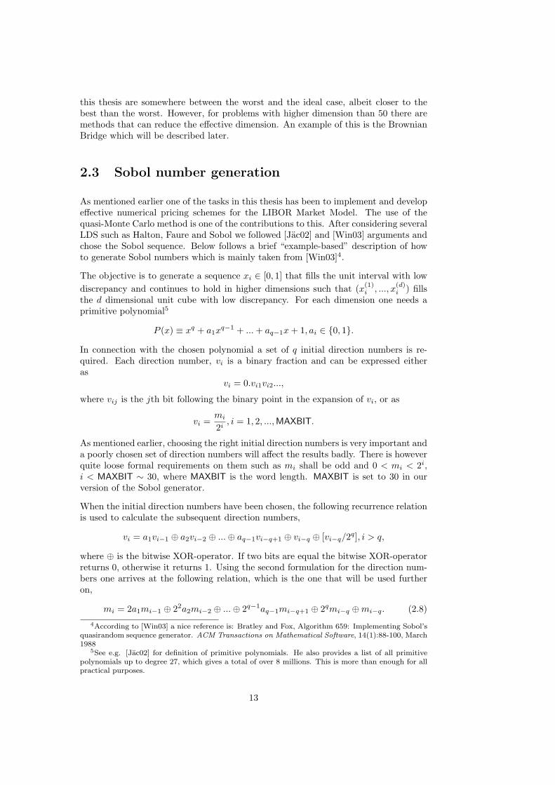
2.3 Sobol number generation
As mentioned earlier one of the tasks in this thesis has been to implement and developeffective numerical pricing schemes for the LIBOR Market Model. The use of thequasi-Monte Carlo method is one of the contributions to this. After considering severalLDS such as Halton, Faure and Sobol we followed [Jac02] and [Win03] arguments andchose the Sobol sequence. Below follows a brief “example-based” description of howto generate Sobol numbers which is mainly taken from [Win03]4.
The objective is to generate a sequence xi ∈ [0, 1] that fills the unit interval with lowdiscrepancy and continues to hold in higher dimensions such that (x(1)
i , ..., x(d)i ) fills
the d dimensional unit cube with low discrepancy. For each dimension one needs aprimitive polynomial5
P (x) ≡ xq + a1xq−1 + ...+ aq−1x+ 1, ai ∈ 0, 1.
In connection with the chosen polynomial a set of q initial direction numbers is re-quired. Each direction number, vi is a binary fraction and can be expressed eitheras
vi = 0.vi1vi2...,
where vij is the jth bit following the binary point in the expansion of vi, or as
vi =mi
2i, i = 1, 2, ...,MAXBIT.
As mentioned earlier, choosing the right initial direction numbers is very important anda poorly chosen set of direction numbers will affect the results badly. There is howeverquite loose formal requirements on them such as mi shall be odd and 0 < mi < 2i,i < MAXBIT ∼ 30, where MAXBIT is the word length. MAXBIT is set to 30 in ourversion of the Sobol generator.
When the initial direction numbers have been chosen, the following recurrence relationis used to calculate the subsequent direction numbers,
vi = a1vi−1 ⊕ a2vi−2 ⊕ ...⊕ aq−1vi−q+1 ⊕ vi−q ⊕ [vi−q/2q], i > q,
where ⊕ is the bitwise XOR-operator. If two bits are equal the bitwise XOR-operatorreturns 0, otherwise it returns 1. Using the second formulation for the direction num-bers one arrives at the following relation, which is the one that will be used furtheron,
mi = 2a1mi−1 ⊕ 22a2mi−2 ⊕ ...⊕ 2q−1aq−1mi−q+1 ⊕ 2qmi−q ⊕mi−q. (2.8)
4According to [Win03] a nice reference is: Bratley and Fox, Algorithm 659: Implementing Sobol’squasirandom sequence generator. ACM Transactions on Mathematical Software, 14(1):88-100, March1988
5See e.g. [Jac02] for definition of primitive polynomials. He also provides a list of all primitivepolynomials up to degree 27, which gives a total of over 8 millions. This is more than enough for allpractical purposes.
13

One can now present an example of how a sequence can be generated. The firstthing that needs to be done is to choose a primitive polynomial and initial directionnumbers for the dimension one would like to generate numbers in. In order to generatethe fourth dimension of the Sobol sequence start, e.g., with the primitive polynomial
P (x) = x3 + x2 + 1. (2.9)
and choose a set of initial direction numbers as,
i 1 2 3mi 1 1 5vi 0.1 0.01 0.101
Table 2.1: Freely chosen initial direction numbers. Note that the vi, of course, is inbinary form.
The next three direction numbers are generated from equation (2.8) which, for thispolynomial, looks like
mi = 2mi−1 ⊕ 8mi−3 ⊕mi−3. (2.10)
This relation yields
m4 = 10 ⊕ 8 ⊕ 1= 1010 ⊕ 1000 ⊕ 01 in binary= 0011 in binary= 3
m5 = 6 ⊕ 8 ⊕ 1= 110 ⊕ 1000 ⊕ 01 in binary= 1111 in binary= 15
m6 = 30 ⊕ 40 ⊕ 5= 11110 ⊕ 101000 ⊕ 101 in binary= 110011 in binary= 51
i 4 5 6mi 3 15 51vi 0.0011 0.01111 0.110011
Table 2.2: Calculated direction numbers from the recurrence relation. Note that thevi, of course, is in binary form.
One can now generate the first variables in the fourth dimension of a Sobol sequence.Sobols originally proposed method for generating the sequence was quite slow. Themethod was therefore enhanced by Antonov and Saleev who used a relation called theGray code and proposed a much faster way to obtain the sequence,
xn+1 = xn ⊕ vc, x0 = 0, (2.11)
14

where c is the position of the rightmost zero-bit in the binary representation of n.The first values of the Sobol sequence based on the polynomial (2.9) and the directionnumbers in tables 2.1 and 2.2 are then
Initialisation x0 = 0.0n = 0 in binaryc = 1
Step 1: x1 = x0 ⊕ v1 = 0.0⊕ 0.1 in binary= 0.1 in binary= 0.5n = 01 in binary, soc = 2
Step 2: x2 = x1 ⊕ v2 = 0.1⊕ 0.01 in binary= 0.11 in binary= 0.75n = 10 in binary, soc = 1
Step 3: x3 = x2 ⊕ v1 = 0.11⊕ 0.1 in binary= 0.01 in binary= 0.25n = 11 in binary, soc = 3
Step 4: x4 = x3 ⊕ v3 = 0.01⊕ 0.0011 in binary= 0.111 in binary= 0.875n = 100 in binaryc = 1
The sequence then continues with 0.375, 0.125, 0.625, ...
2.4 Path construction
When uniform sequences are generated either by a pseudo-random or low-discrepancygenerator one will in general use them to create paths of normally distributed variates,the Brownian motions.
2.4.1 Incremental path construction
The most straightforward and simple method to construct samples of a Brownianmotion (BM) is through the standard incremental way,
Wti+1 = Wti +
√∆t · νi, i = 1, ..., T, νi ∼ N(0, 1)
Wt0 = 0.
15

Using this method it is also quite simple to generate several correlated Brownianmotions
W 1t+1
W 2t+1
...Wmt+1
=
W 1t
W 2t
...Wmt
+ A
√∆t
ν1
ν2
...νm
, (2.12)
where A is the pseudo-square root obtained by Cholesky decomposition of the covari-ance matrix C, i.e. a lower triangular matrix satisfying AAT = C.
The incremental method works perfectly when dealing with pseudo-random variates.However, when constructing variates with the Sobol method the behavior in higherdimensions is not completely satisfying. One big disadvantage with the incrementalconstruction is that the variance due to variate νi of the path is decreasing very slowly.This implies that the higher dimensional variates determines a quite large part of thetotal variance of the path. It would therefore be interesting to find a path constructionmethod for which the lower dimensional variates determines an as large as possiblepart of the total variance. One method that has this feature is the Brownian Bridgepath construction, see [Caf98],[Jac02] or [Win03].
2.4.2 Brownian Bridge path construction
With the Brownian Bridge path construction a very large part of the total varianceis contributed by the first 2 dimensions of the Sobol sequence6. Instead of addingthe increments with the same timestep size ∆t the Brownian Bridge construction firstdetermines the last value in the path WT , then using this value, and W0 = 0, itgenerates WT/2. It then proceeds in the same way until all points are filled. Thewhole procedure is illustrated below
WT =√Tν1
WT/2 = 12WT +
√T
2 ν2
WT/4 = 12WT/2 +
√2T4 ν3
...
W(m−1)T/m = 12 (W(m−2)T/m +WT ) +
√T
2mνm.
(2.13)
The resulting normal increments can then be backed out from the path using
νBBi =Wti+1 −Wti√ti+1 − ti .
2.4.3 Several Brownian motions from Sobol sequences
When constructing multi-factor or multi-asset paths with variates from a Sobol se-quence one has to be careful. Since the lower dimensions display better equidistri-bution one can not create the first Brownian motion path from the first variates, the
6According to [Win03] 90% of the variance is contributed by the first 2 dimensions. This seems alittle bit too high and a better guess might be around 75%.
16

second path with the following variates and so on because then the last paths wouldbe created by high dimension variates only and will get very bad properties.
One salvation of this problem is to divide the Sobol sequence into smaller groupswhere each group contains variates both from lower and higher dimensions. Considerthe ith d dimensional Sobol sequence (x(1)
i , x(2)i , x
(3)i , ..., x
(d−2)i , x
(d−1)i , x
(d)i ). In the
incremental path construction one should use variates x(1)i , x
(4)i , ... in path 1, variates
x(2)i , x
(5)i , ... in path 2 and so on in order to generate the ith sample of the Brownian
Motion. The Brownian bridge construction will be based on the same idea. If one, forexample, would like to create three different paths build them up by sampling fromevery third dimension.
(x
(1)i , x
(4)i , ...x
(d−2)i
)→(...,W i1
T/2(xi(4)), ...,W i1T (x(1)
i ))
(x
(2)i , x
(2)i , ...x
(d−1)i
)→(...,W i2
T/2(xi(5)), ...,W i2T (x(2)
i ))
(x
(3)i , x
(6)i , ...x
(d)i
)→(...,W i3
T/2(xi(6)), ...,W i3T (x(3)
i )) (2.14)
2.5 Implementation of the Sobol sequence generator
The Sobol sequence generator implemented and used in this thesis is based on theC program in [PTVF92]. Since the polynomials and initial direction numbers in thisgenerator only provides sequences up to six dimensions and this thesis deals withproblems with dimensions higher than hundred the generator has to be extended.In order to do so primitive polynomials from the almost unlimited list provided in[Jac02] are used. [Jac02] also provides carefully selected initial direction numbers upto dimension 31. We therefore start with these ones and then continues with the initialnumbers provided by [Win03] in order to design Sobol sequences up to 160 dimensions.
As mentioned before the implemented Sobol sequence generator should work very wellin dimensions under 50 and also reasonable well in higher dimensions. Test cases withthe Brownian Bridge construction shows that in practise a significant convergenceimprovement is achieved also in high dimensions. Summarising yields that by carefulselection of the initialisation numbers in the Sobol sequence generator and the use ofthe Brownian Bridge path construction the convergence rate is almost independent ofthe dimension in practise as opposed to the theoretical convergence rate introducedearlier. See chapter 6 for some results.
17

CHAPTER
THREE
The LIBOR market model
This chapter will begin exploring the LIBOR market model (LMM). It will start bydescribing the dynamics of the forward rates and determining the arbitrage free driftfunction. Further on discretisation of the forward rate dynamics and effective numer-ical simulation schemes will be described. The next chapter will thereafter categorisesome of the derivatives that can be handled by the LMM and describe fast and correctpricing schemes. Attractive references for further studies and/or other presentationsare Rebonato, [Reb02], Brigo & Mercurio, [BM01], Hull & White, [HW99] and Pelsser,[Pel00].
Definitions of the interest rate market securities are given in Appendix B. Figure (3.1)might provide a way to remember which quantities that are modelled.
t0 t3t2t1 t4 t
spot(t0,t1 ) f(t0 ,t1 ,t2 ) f(t0 ,t2 ,t3 ) f(t0, t3, t4 )
spot(t0,t2 ) f(t0 ,t2 ,t4 )
Z(t, t2 )
Z(t, t3 )
Figure 3.1: The spot and forward rates for two forward rate structures with differenttenor lengths and two of the corresponding zero coupon bonds.
As shown in Appendix B a forward rate structure is built up by one spot rate and nforward rates with reset dates
t0, t1, t2, ...tn−1, tn.The forward rates are defined as
f(t, ti, ti + τi)τi =Z(t, ti)− Z(t, ti + τi)
Z(t, ti + τi)
where Z(t, ti) is the price process of the zero-coupon discount bond that pays 1 attime ti and τi is the tenor of the forward rate that resets at time ti.
18

3.1 Forward rate dynamics in the LMM
This section tries to derive a comprehensive version of the forward rate dynamics inthe LIBOR market model. The following notation will be used:
fi(t) Forward rate observed at time t for the period ti → ti+1 withthe compounding period τi = ti+1 − ti.See figure (3.1) for a graphic view and Appendix B for definitions.
dWk(t) The k:th standard Brownian motion at time t.σik(t) The instantaneous volatility function of the i:th forward rate
for the k:th Brownian motion at time tµi The drift parameter. Can depend on both time and on the forward
rates themselves. It is therefore denoted without arguments for now.
The forward rate dynamics is described by the m-dimensional diffusion equation1,
dfi(t)fi(t)
= µidt+m∑
k=1
σik(t)dWk(t), (3.1)
where the Brownian motions, dWk(t), k = 1, ..m are modelled as orthogonal i.e. thecorrelation between them is zero. The σik(t)s can be linked with the total volatilityof the i:th forward rate. In order to do this start by, as in Appendix B when pric-ing swaptions and caplets, distinguishing between the time-dependent instantaneousvolatility for the forward rate resetting at time ti, σi(t), and its implied “average”volatility given by the Black-76 formula,
σ2Black(ti)ti =
∫ ti
0
σ2i (s)ds. (3.2)
In the above expression for the forward rate dynamics, σik(t) is denoted as the volatilitycontribution to the ith forward rate given by the kth Brownian motion. Using thestandard formula for calculating the variance of the forward rate it is straightforwardto show that the total instantaneous volatility of the forward rate σi(t) and the σik(t)sare related by
σ2i (t) =
m∑
k=1
σ2ik(t). (3.3)
Dividing and multiplying each loading, σik(t), with the instantaneous volatility of theith forward rate and using equation (3.3) gives
dfi(t)fi(t)
= µidt+ σi(t)m∑
k=1
σik(t)σi(t)
dWk(t)
= µidt+ σi(t)m∑
k=1
σik(t)√∑mk=1 σ
2ik(t)
dWk(t)
≡ µidt+ σi(t)m∑
k=1
bik(t)dWk(t)
where
bik(t) =σik(t)√∑mk=1 σ
2ik(t)
. (3.4)
1Note that this means that m factors are driving all the forward rates i.e. the same Brownianmotions are used to evolve both fi and fj , i 6= j
19

This formulation is very useful since it decomposes the orthogonal shocks of the forwardrates into two distinct components. The first component, σi(t) only depends on thetotal volatility of the ith forward rate. For correct pricing of the associated caplet thishas to be chosen according to (3.2). Also note that by definition,
m∑
k=1
b2ik(t) = 1, (3.5)
which implies that this component will not affect the caplet pricing at all and mightinstead be used to contain the models information about the correlation structurebetween the forward rates. The above expression for the forward rate dynamics seemsvery appealing and is the formulation that is used in this thesis.
3.2 The drift function
This section will derive the arbitrage free drift of the forward rates under differentmeasures. In order to understand this better Appendix A, or any of the referencesgiven there, should provide enough theory. Start by consider the Equivalent MartingaleMeasure (EMM) Qi+1 associated with the discount bond Z(t, ti+1). Rewriting theexpression for the forward rate gives
fi(t)Z(t, ti+1) =Z(t, ti)− Z(t, ti+1)
τi.
Notice that fi(t)Z(t, ti+1) is a tradable asset since it can be replicated by buying andselling two bonds. As such, it can be divided with the numeraire Z(t, ti+1) which, bydefinition of a martingale measure, gives a martingale under Qi+1. Hence, shortingthe two bonds implies that fi(t) is a martingale under Qi+1. The diffusion processabove can, in the martingale case, be written as2
dfi(t)fi(t)
= σi(t)dW i+1(t),
where dW i+1(t) is a Brownian motion under Qi+1. However, applying the reasoningabove to the forward rate fj(t), j 6= i one notices that fj(t)Z(t, ti+1) is not a tradableasset and hence under the measure Qi+1 only fi(t) is a martingale.
In a non-trivial pricing case one is interested in evolving all forward rates under thesame measure. In order to do so one has to know the diffusion equation for all theforward rates under that measure. It is above motivated that under a certain measureone forward rate is a martingale, i.e. it has driftless diffusion equation, but all otherforward rates has non-zero drift terms. In Appendix A it is shown that a change ofmeasure only changes the drift term whether the diffusion term remains unaffected. Inorder to determine the drift term under Qi+1 for the Qi-martingale fi−1 consider thechange of measure dQi/dQi+1. Once again, following following the artillery introducedin Appendix A the Radon-Nikodym derivative ρ(t) is given by
dQi
dQi+1= ρ(t) =
Z(t, ti)/Z(0, ti)Z(t, ti+1)/Z(0, ti+1)
=Z(0, ti+1)Z(0, ti)
(1 + τifi(t)). (3.6)
2A one-factor model is chosen in order to make the expressions less greasy. However, the resultingdrifts will look exactly the same, just put in the summation sign in order extend it to a multi-factorcase.
20

To be able to use Girsanovs theorem one needs to find the process k(t) such that
ρ(t) = exp∫ t
0
k(s)dW i+1(s)− 12
∫ t
0
k2(s)ds. (3.7)
An application of Itos lemma on (3.7) shows that
dρ(t) = ρ(t)k(t)dW i+1(t), (3.8)
hence k(t) can be seen as the volatility of the Radon-Nikodym derivative ρ(t). However,applying Itos lemma on (3.6) and remembering the driftless diffusion equation for fi(t)under Qi+1 yields
dρ(t) =τiσi(t)fi(t)1 + τifi(t)
ρ(t)dW i+1(t) (3.9)
Hence, equating (3.8) and (3.9) one can identify k(t) = τiσi(t)fi(t)1+τifi(t)
which, throughGirsanovs theorem, gives that a change of measure from Qi to Qi+1 affects the Qi-Brownian motion dW i(t) as
dW i(t) = dW i+1(t)− τiσi(t)fi(t)1 + τifi(t)
dt (3.10)
The diffusion equation for fi−1(t) under the measure Qi+1 can then be written as
dfi−1(t)fi−1(t)
= −τiσi(t)fi(t)1 + τifi(t)
σi−1(t)dt+ σi−1(t)dW i+1(t).
If one splits the volatility function σi(t) into one volatility contribution part and onecorrelation contribution part one may instead of σk(t)σl(t) write σk(t)σl(t)ρkl(t) whereρkl(t) is the correlation function and, for simplicity, the old volatility function notationhas been used for the new correlation-independent volatility functions.
Using (3.10) repeatedly it is straightforward to show that when choosing the EMMQj+1 associated with the numeraire Z(t, tj+1) the trend term of fi(t), for forward ratesresetting before tj , in general follows
µi(f(t), t) = −σi(t)j∑
k=i+1
σk(t)ρik(t)fk(t)τk1 + fk(t)τk
i < j. (3.11)
Applying exactly the same arguments to the case i > j gives
µi(f(t), t) = σi(t)i∑
k=j+1
σk(t)ρik(t)fk(t)τk1 + fk(t)τk
i > j. (3.12)
A first glimpse about the above equations yields that the drift terms are functions ofboth time and the, at a future time t, stochastic forward rates fk(t). The stochasticnature of the drift term will impose some pricing problems but, as shown later, the driftterm can be well approximated by deterministic functions via a Predictor-Correctormethod.
It might be interesting to compare the forward rate dynamics and the form of thedrift function with the HJM instantaneous forward rate dynamics. The last sectionin Appendix B shows that when taking the limit as the tenors tend towards zero theLMM and the HJM forward rate dynamics coincide.
21

A first attempt to price interest rate derivatives
Since the previous section has been quite abstract and the probability that the readerfeels a bit lost is rather high it might be time for a first look about how to use theLMM forward rate dynamics to price interest rate derivatives.
The dynamics of the forward rates were derived above as
dfifi
= µi(f(t), t)dt+ σi(t)m∑
k=1
bik(t)dWk.
Since the drift terms derived above are clearly state-dependent and thus indirectlystochastic one is forced to use a numerical scheme to solve the above equation alongany path. Approximating the forward rates as constant over the time step t→ t+ ∆tone is able to use the forward Euler method for integration from t to t+ ∆t
fEuleri (f(t+ ∆t), t+ ∆t) = fi(t) + fi(t) · µi(f(t), t)∆t+ fi(t) · σi(t) ·m∑
k=1
bik(t)zk√
∆t,
with zk being m independent normal variates3.
Now put yourself a time t0 and choose the zero-coupon bond maturing at time t1 asnumeraire. With this numeraire the drift term for all the forward rates will behaveas in the case i > j. Consider a derivative whose payoff depends on the forward ratestructure at time t1. In order to price this derivative one just have to move the forwardrate structure forward to time t1 using the Euler scheme above, determine the payoffand discount it back to time t0. The next chapter discuss several improvements andvariants of this, however, the procedure outlined above is the fundamental base in allthe pricing methods.
3.3 Discretising the forward rate equation
This section will discuss the very important issue of discretising the forward rateequation in order to evolve it forward in time. In addition to the references alreadygiven in this section the paper by Hunter et al, [HJJ01] is some very fruitful reading.By the aid of Ito integration the equation can be written4.
fi(t) = fi(0)exp
∫ t
0
[µi(f , s)− 12σ2i (s)]ds+
∫ t
0
σi(s)m∑
k=1
bik(s)dWk
. (3.13)
Unfortunately, it is not a priori known how to analytically integrate the quantity underthe left integral sign over a finite time interval since the integral is not a pure functionof time, it also depends on the state of the forward rates themselves. However, if one
3Note that this scheme implies using a normal instead of log-normal distribution for the evolutionof the forward rates over this time step. The next section will show log-normal numerical schemes
4It is throughout this thesis assumed that the instantaneous volatility function is a function oftime only. When trying to extend the LMM to recover the smile effect volatility functions dependingon the level of the forward rate is a popular choice.
22

could write5
∫ t
0
i∑
k=j+1
σi(s)σk(s)ρik(s)fk(s)τk1 + fk(s)τk
ds ≈i∑
k=j+1
fk(0)τk1 + fk(0)τk
∫ t
0
σi(s)σk(s)ρik(s)ds,
(3.14)i.e. if one approximates the stochastic term fk(t)τk/[1 +fk(t)τk] as piecewise constantthen the drift integrals would be computable. This approximation is the most crucialapproximation one has to do when evolving the forward rates. The approximation canbe shown to work fine when taking smaller steps, such as three or six months, but ifone wants to take longer steps it might be too crude. Due to this and in order to reducetime consumption two different methods for evolving the forward rate structure, theshort step method and the long step method, is developed.
3.3.1 The short step method
The short step method evolves the forward rate structure so that exactly one forwardrate will come to its reset time at every step, i.e. in a 3-month forward rate structure3-month long steps will be taken.
In order to define a log-normal discretisation of the forward rate equation it is useful towork in log space. Defining Yi(t) = lnfi(t) yields the system of stochastic differentialequations
dYi(t) =[µi(Y(t), t)− 1
2σ2i (t)
]dt+ σi(t)
m∑
k=1
bik(t)dWk(t).
As before, assuming piecewise constant drift makes it possible to take a single Eulerstep
Y Ei (t) = Yi(0) +[µi(Y(0), 0)− 1
2σ2i (0)
]t+ σi(0)
m∑
k=1
bik(0)√
(t)zk
where the zks are uncorrelated N(0, 1) variables. There is one direct improvementof this discretisation. From equation (3.14) one realises that instead of ignoring theintegral on the right hand side of the equation by taking the time 0 values of the σsand ρ it should be calculated, i.e. put
Cik =∫ t
0
σi(s)σk(s)ρik(s)ds. (3.15)
5Suppose a measure with a discount bond maturing before all forward rates are chosen as nu-meraire.
23

This yields that the drift term in the case i > j can be written as, (the same thingapplies, of course, in the case j > i)
µi(f(0), C) =i∑
k=j+1
fk(0)τk1 + fk(0)τk
Cik,
or in log space as
µi(Y(0), C) =i∑
k=j+1
Yk(0)τk1 + Yk(0)τk
Cik. (3.16)
Using this yields what will be referred to as the log-Euler scheme,
Y Ei (t) = Yi(0) +[µi(Y(0), C)− 1
2Cii
]+ σi(0)
m∑
k=1
bik(0)√tzk. (3.17)
This scheme can be shown to be accurate enough ( see e.g.[Reb02] or [HJJ00]) inmost practical cases. However, one might not be completely satisfied with the ap-proximation of piecewise constant drift. Luckily there are methods to improve thisapproximation. In [HJJ00] a very appealing method is presented which they call thePredictor-Corrector(PC) method. The P-C method is easy to understand and in theirpaper it is shown that it will produce very accurate values also in some more extremecases. The recipe for the method is
The Predictor-Corrector recipe1. Evolve the logarithms of the forward rates with piecewise constant drifts
according to the log-Euler scheme (3.17).2. Compute the drifts at the terminal time with the so evolved forward rates.3. Average the initially calculated drift coefficient with the newly computed ones.4. Re-evolve using the same normal variates as initially but using the new
Predictor-Corrector drift terms.
This recipe yields the scheme below which will be referred to as the PC-log Eulerscheme
Yi(t) = Yi(0) +12[µi(YE(t), C) + µ(Y(0), C)− Cii
]+ σi(0)
m∑
k=1
bik(0)zk (3.18)
Since it is so easy to use and always will perform as good as or better than the standardlog-Euler scheme the PC-log Euler scheme will be used in all calculations.
Given this, it is possible to describe the short step method in detail. Consider, as be-fore, a forward rate structure consisting of one spot rate(the rate between t0 and t1) andN forward rates. The reset times of this structure are (t0, t0+τ0 = t1, ..., tN−1+τN−1 =tN ) and the payoff times are t1, t2, ..., tN+1. Suppose one is interested in taking n < Nsteps forward in time to time tn(one might have a derivative whose payoff depends onthe information available at time tn). Remember that choosing the natural payoff ofthe short rate i.e. the discount bond maturing at t1 all of the forward rates will havedrift terms as in the j < i case. The short step method can now be described as
24

The short step method recipe0. Choose Z(0, t1) as numeraire. Put j = 0.1. Evolve the logarithms of the forward rates with the PC-log Euler scheme
from time tj to time tj+1 using the j < i drift.2a. Note that when standing at time tj+1 the forward rate f(tj+1, tj+1, tj+2)
has become a spot rate instead of a forward rate and hence the initialforward rate structure now consists of N − 1 forward rates.
2b. If not tj+1 is the final destination go to 3, else go to 5.3 Choose the natural payoff of the spot rate f(tj+1, tj+1, tj+2)
as numeraire, that is choose Z(tj+1, tj+2),4. Set j = j + 1 and go to 1.5. The information gathered when standing at the final destination(in this
case after taking N steps) is shown in the table below.
spot(t0) f1(t0) f2(t0) . . . fN−1(t0) fN (t0)spot(t1) f2(t1) . . . fN−1(t1) fN (t1)
spot(t2) . . . fN−1(t2) fN (t2). . .
......
spot(tN−1) fN (tN−1)spot(tN )
Note that with this information one is able to evaluate the payoffof path dependent derivatives that depends on the way taken to arriveat the final destination. Also note that, of course, it is not possibleto take more number of steps than the number of forward rates in theinitial structure.
Definition 3 (Short step filtration) The information gathered when moved to timet using the short step method will from now on be called the short step filtration,Fsst . Derivatives that can be priced by the short step method can hence be called Fsst -measurable.
The next chapter will discuss how to determine derivative prices with the short stepmethod. At this time just note that the information gathered with this method shouldbe enough to price many different types of derivatives.
The short step method will produce payoff and prices along one path in a MonteCarlo computation. Since one is taking quite many steps with this method runninga Monte Carlo computation can be time consuming. When dealing with derivativeswhose payoff only depends on the information available at the final destination onemight consider taking one long step direct to the final destination and speeding up theMC simulation considerably. A method for doing this is described in the next section.
3.3.2 The long step method
The idea with the long step method is that when a derivative does not depend on theinformation available at one point in time, that point does not have to be visited. Thiscan imply very long steps and not using the Predictor-Corrector method described inthe previous section might produce too inaccurate results. It is in [HJJ00] argued that
25

with the P-C method it is, in fact, possible to take steps as long as 10 or even 20 yearswith good precision.
The long step method starts by choosing as numeraire any of the discount bondsmaturing at one of the reset dates of the rates. The drift term for fi will then begiven as shown earlier depending on whether i is bigger than, equal to or less thanj. As before use will not be made of the initial values of the volatilities but insteadthe terminal covariance matrix Cij as in equation (3.15). There is though a slightlydifferent situation arising here than in the short step method. There the matrix Cijwas calculated between the reset dates of the rates and therefore all rates considered( N rates in the interval (0, t1), N − 1 rates in (t1, t2) and so on) were still “alive”.However, when taking a step longer than the tenor period of the first forward ratethen forward rates will have come to their reset dates on the way. Suppose one wouldlike to take a step to time tn, a time when several forward rates already has reset.When calculating the matrix Cij it is therefore not possible to evaluate the integralup to time tn for all is and js. The solution to this problem is however quite simple.Letting σi(t) = 0 if t is greater than the reset date of the corresponding rate yields avalid terminal correlation matrix. More explicitly if the reset date for fi is ti and onewants to calculate the (total) terminal covariance between fi and fj where j > i thenset
TOTCij =∫ ti
0
σi(s)σj(s)ρij(s)ds. (3.19)
In fact, this is exactly the same as calculating the C matrices for each short step un-derlying the long step and then sum them6. This is the reason why, for the long stepmethod, the terminal covariance matrix is called TOTC (TOtal Terminal Covariance-matrix).
The long step method hence also uses the PC-log Euler scheme but instead of theC-matrix it uses the TOTC-matrix. The information gathered when taking a longstep up to time tn can then be viewed as
spot(t0)spot(t1)
. . .spot(tn) fn+1(tn) . . . fN (tn)
This implies the possibility to price and discount derivatives depending on the infor-mation at time tn and the realised spot rates but not on any more information at anyearlier time.
Definition 4 (Long step filtration) The information gathered when moved to timet using the long step method will from now on be called the long step filtration, F lst .Derivatives that can be priced by the long step method can hence be called F lst -measurable.Note that the long step filtration is a subset of the short step filtration.
Using as many factor as forward rates
When using the short step method, evolving the forward rate structure using too manyfactors is, in general, hopelessly slow. Since one usually takes a large number of steps
6The reader is encourage to understand why it is so. Note that the dimensions of the C matricesis n, n− 1,... and so on for each step forward in time.
26

with the short step method, drawing many normally distributed shocks at each stepwill require quite some work.7.
With the long step method it is often possible to use as many driving factors as thereare rates. Taking only one long step forward in time, the time-penalty when using alarge number of factors is not as large as when taken many short steps. Using theCholesky decomposition method when creating the Brownian Motions as described insection 2.1.4 the following PC-log Euler scheme is obtained
Yi(t) = Yi(0) +12[µi(YE(t), TOTC) + µ(Y(0), TOTC)− TOTCii
]+
N∑
k=1
Aikzk.
(3.20)Remember from section 2.1.4 that Aik is the pseudo-square root of the Cholesky de-composition and satisfies
TOTCij =N∑
k=1
AikAjk.
3.4 A swap rate based market model
When there is an interest in pricing swap rate based derivatives one might considermodelling the swap rate instead of the forward rate. The swap rate model can bethreaten exactly as the forward rate model and, as shown further on, when a forwardrate implementation prices caplets perfectly the swap rate implementation insteadprices swaptions.
There is however two main drawbacks with this approach. The first is that the no-arbitrage drifts will be considerably more involved and computationally demanding andrequire rather careful numerical handling. The second drawback is that the inputs tothe model are less directly related to market observable quantities than the forwardrate based version. Because of this traders seems to have less well-informed ideasabout the instantaneous volatility and correlation function for the swap rates and itwill hence be hard to perform a satisfying calibration.
As shown further on there are well developed methods for calibrating a forward ratebased model also to swaption prices. Since these methods seems to work very fine andbecause of the drawbacks mentioned above, a swap rate based market model will notbe considered. Instead a forward rate based model calibrated against swaption priceswill be used for pricing swap rate based products.
7Suppose one is taken 30 steps forward in time. For an n-factor model the number of drawsrequired in each realisation is n · 30. Comparing a 2-factor model with a 30-factor model one directlyrealises that there will be a quite large difference in MC computation time.
27

CHAPTER
FOUR
Characterising and pricing LIBOR derivatives
This chapter will provide information about the types of derivatives that can be han-dled by the LMM and how to price them in an effective and correct way. The deriva-tives will be categorised according to if they can be handled by the short step and/orlong step method for evolving the forward rates introduced earlier. Effort will be madeto give the reader a feeling for the measure implied pricing techniques that has to beused when dealing with the LMM.
4.1 Characterising LIBOR derivatives classes
This section will generalise the types of derivatives that can be handled with theLMM into 3 different groups; single-look, path-dependent and multi-look compoundproducts. It will be argued that single look derivatives always can be handled bythe long step method whereas some path-dependent derivatives can be handled bythe long step and some with the short step depending on the features of the path.Pricing multi-look compound products are not dealt with in this thesis but since itis an important group of derivatives that can be handled by the LMM they will bediscussed shortly and some references for further studies will be given.
Single look derivativesThe payoff of single-look options is completely determined by the values of a forwardrate structure at a single future time Texp. Remembering the information gatheredby the long step evolution one realises that the information should be enough to bothevaluate and discount the payoff i.e. single look derivatives are both Fsst - and F lst -measurable. Typical single look type derivatives are European Swaptions and Caps.
Path-dependent derivativesFor path-dependent derivatives the payoff occurring at time TN depends on the real-isation of a series of forward rates on reset dates Ti, 1 ≤ N . In order to distinguishbetween path-dependent derivatives that are Fsst - and F lst -measurable they can bedivided into two groups.
28

1. Path dependent derivatives depending on the joint realisations of forwardrates which, by the time of each price-sensitive events have already cometo their own reset dates, i.e. they are F lst measurable.
2. Path dependent derivatives whose payoffs depend on the joint realisationof forward rates for which some of them might not have reset yet, i.e.they are Fsst measurable.
Multi look compound productsThe prime example of a multi-look compound derivative is the Bermudan swaption.A Bermudan swaption is an option to enter a swap on a number of different datesin the future. A Bermudan swaption is denoted as X-non-call-Y which means thatthe first exercise opportunity is Y years after inception and that the final maturitydate is X, regardless of when the option is exercised. What makes a Bermudan swap-tion (and other Multi-look compound products) difficult to price is the fact that atevery exercise opportunity date one has to decide whether the value of exercising ishigher than the expected profit of not exercising the option. The standard way toprice these kind of options is the lattice-approach but there is one big problem withthis. The state-dependent drift terms in the forward rate diffusion equation implies anon-recombining lattice. This non-recombining property makes the lattice grow expo-nentially in size at every timestep and it therefore demands a lot of computer powerand clever implementation to price the derivative this way. However, it is possible andJackel, [Jac00a], presents a possible way.
One possible route to circumvent this problem is to force the recombination to takeplace as made in Pelsser et al, [HKP00]. Another, and probably the most popular,way is to try to estimate an optimal exercise boundary i.e. to try to find a function1
which, at each exercise date, acts like a trigger and decides whether or not to exercise.This makes it possible to price the Bermudan swaption by ordinary Monte Carlointegration as before. Popular approaches are made by e.g. Longstaff & Schwartz,[LS98], Andersen, [And99] and Jackel, [Jac00b]. These approaches are quite generaland might work fine also for American type options.
4.2 Effective pricing schemes
This section will deal with pricing derivatives with the short and long step methodsrespectively. The goal is to explain the impact of the measure induced pricing impli-cations and help the reader choose the most effective scheme for his/hers problem. Inorder to get a feeling for all this, this section will begin with a general example which,perhaps, at first sight might seem a bit cumbersome. However, a solid understandingof this example implies that the reader should not have any problem understandingthe pricing schemes presented later or building his/her own schemes. A measure usedin the example and by the long step method is the Terminal measure.
Definition 5 (The Terminal measure) Given a set of times t0, t1, ..., tN , tN+1,ti+1 = ti+τi. The terminal measure, QN+1, can be defined as the EMM with the zero-coupon bond Z(t, tN+1), as numeraire. Under this measure all forward rates with resetdates up to tN−1 has drifts as in the i < j case and the forward rate f(t, TN , tN+1)
1This function might depend on the value of exercising, the forward rate structure and otherinformation that might be useful.
29

has zero drift. Moreover, given a price process π(t),
π(t)Z(t, tN+1)
,
is a martingale and hence
π(t0) = Z(t0, tN+1)EQN+1
[π(tn)
Z(tn, tN+1)|Ft0
].
If one put
π′(tn) =π(tn)
Z(tn, tN+1),
where π′(tn), as described in Appendix A, is denoted as a relative price process at timetn, one has
π(t0) = Z(t0, tN+1)EQN+1
[π′(tn)|Ft0 ] .
Now suppose one is interested in pricing a caplet2 whose payoff is determined at tnand received at tn+1. In order to price this with the above formula its relative priceprocess has to be decided. Below is three, in expectation, equal ways of doing thisstated, depending on which time one is considering. The first, and perhaps mostappealing, is the relative price process at time tn+1
π′(tn+1) =π(tn+1)
Z(tn+1, tN+1). (4.1)
Since the payoff is determined at time tn one might also determine the relative priceat time tn,
π′(tn) =π(tn+1)Z(tn, tn+1)
Z(tn, tN+1). (4.2)
Note that for a given path of simulated LIBOR rates these expressions need not bethe same, but they are equivalent in martingale pricing sense,
π′(tn) = EQN+1
[π′(tn+1)|Ftn ] .
It is also possible to reinvest the payoff from time tn+1 until tN+1 into the depositrate,
π(tN+1) = π(tn+1)N∏
k=n+1
(1 + τkf(tk, tk, tk+1)) = π′(tN+1). (4.3)
Also this is equal to the other two ways in martingale pricing sense,
π′(tn) = EQN+1 [π′(tN+1)|Ftn ].
The following example based on an example in [Pel00] might illustrate the abovetheory.
Assume a LIBOR Market Model with semi-annual rates, ti = 0.5i, i = 0, ...4. Suppose oneis interested in pricing a forward starting interest rate cap with expiry date t1 and maturitydate t5 = t4 + 0.5. Suppose the following realisation of rates is generated with the short stepmethod under the terminal measure,
2See Appendix B for a definition of caps and caplets
30

Realised rates
t0 5.000% 5.000% 5.000% 5.000% 5.000%t1 4.181% 4.182% 4.183% 4.184%t2 5.125% 5.128% 5.130%t3 4.715% 4.719%t4 4.916%
Discount factors
t0 0.976 0.952 0.929 0.901 0.884t1 0.978 0.959 0.940 0.921t2 0.975 0.951 0.927t3 0.977 0.954t4 0.976
The value of the cap with strike 5% at time t5 is the sum of the relative caplet payoffs alongone path. For the path above there is only one strike that is in-the-money namely the oneat time t2 for which the realised rate is 5.125% (remember that this one was called spot(t2)before). The relative value of this caplet can then be calculated as,
π′(t2) = (spot(t2)%− 5%) · 0.5 · Z(t2, t3)/Z(t2, t5) = 0.06575%
orπ′(t3) = (spot(t2)%− 5%) · 0.5/Z(t3, t5) = 0.0655%.
or
π′(t5) = (spot(t2)%− 5%) · 0.5 · (1 + 0.5 · spot(t3)) · (1 + 0.5 · spot(t4)) = 0.06555%.
Remember from before that one now has three, in martingale sense, equivalent estimationsof the relative value of the cap, π′cap, for this particular realisation. Using M number ofrealisations gives an estimate of the Monte Carlo computed value of the cap as
πcap(t0) = Z(t0, t5)
"MXj=1
π′cap(j)M
#.
The theory outlined above is quite general. The section below will define two partic-ulary nice pricing schemes.
4.2.1 The short step method pricing scheme
How to generate the forward rates with the short step method is described in theprevious chapter. One is there using the spot measure.
Definition 6 (The Spot measure) Given a set of times t0, t1, ..., tN , tN+1, ti+1 =ti+τi. The spot measure, Q1, can be defined as the equivalent martingale measure withthe zero-coupon bond Z(t, t1) as numeraire. Under this measure all forward rates thatresets at bond payoff times greater than t1 has drifts as in the i > j case. Moreover,given a price process π(t),
π(t)Z(t, t1)
,
is a martingale and hence
π(t0) = Z(t0, t1)EQ1
[π(t1)|Ft0 ] .
31

Suppose one is interested in pricing a derivative with stochastic payoff X(·) at timetN+1. The price at time t0 expressed in terms of the price at time t1 is given in thedefinition of the sport measure above. Applying this for π(t1), i.e. choose the measureQ2 with Z(t, t2) as numeraire yields,
π(t1) = Z(t1, t2)EQ2 [π(t2)|Ft1 ] .
Repeating this until the payoff time tN+1 for the derivative is reached one has
π(t0) = Z(t0, t1)EQ1[Z(t1, t2)EQ2
[...Z(tN , tN+1)EQN+1 [X(·)|FtN ]|Ft1
] |Ft0].
With the short step method PC-log Euler steps forward in time will be taken and bythis way the discount bonds and expectations will be realised one at a time using thefiltrations Fssti until time tN . This implies that the price π(t0) of the derivative can,for one computation round, be written as
π(t0) =N∏
k=0
11 + spot(tk)τk
X(·). (4.4)
This procedure is very easy to extend for a Fsst -measurable derivative with severalpayoff dates, just discount them one at a time and sum the time t0 values.
In order to price the derivative by Monte Carlo integration one realises that the ex-pectation in the pricing equations are integrals which can be computed as averagesaccording to the theory outlined in chapter two. Suppose that the realisations yieldsthe prices π1(t0), π2(t0), .... The price after N realisations is then estimated by
πMC(t0) =∑Nk=1 π
k(t0)N
. (4.5)
As mentioned before this method is very powerful and (hopefully) quite easy to un-derstand. The main disadvantage is the time consumption. Suppose taking 3-monthssteps 5 years forward in time. For a 2-factor LMM this requires 40 normal variatedraws at each Monte Carlo round and the building of 20 C-matrices. Compared totaking one long step which requires 2 normal variates and 1 C-matrix one quicklyrealises that there is a lot of time to win with the long step approach.
4.2.2 The long step method pricing scheme
As mentioned above it is possible to generate realisations of the rates significantlyfaster by using the long step method. It is also argued that it is unfortunately notpossible to price all kind of derivatives with the long step method, i.e. they are notmeasurable with respect to the filtration F lst . One of the most appealing advantageswith the short step method is that it is fairly easy to understand the discountingprocedure. With the long step method it gets, at least for multi-payoff derivatives, alittle bit more complicated. Let us therefore start with a derivative with one singlepayoff date.
Suppose the payoff at time tN+1 is given by X(·). Start by choosing the Terminalmeasure QN+1, defined above. The value of the derivative can be evaluated by
π(t0)Z(t0, tN+1)
= EQN+1
[π(tN+1)
Z(tN+1, tN+1)|F0
]
32

which yields,π(t0) = Z(t0, tN+1)EQN+1 [X(·)|F0]
Note the difference between the pricing equations in the short and long step method.When using the long step method for pricing a single payoff derivative with a stepdirectly to the payoff date the payoff is determined by the filtration F lst given by thePC-log Euler step. The discount factor is, however, determined by the filtration Ft0 .When using the short step method the filtration Ft0 only discounts the payoffs fromtimes t1 to t0 whereas the filtration Fsst is used for both evaluating the payoffs anddiscounting between the rest of the times.
When dealing with derivatives with several payoff dates this procedure gets a little bitmore complicated. However, the theory outlined in the general case and the exampleabove, will be very useful. Consider a derivative with payoffs Xi(·), Xj(·) and XN+1(·)at times ti, tj and tN+1 respectively. In order to price this with the long step methodchoose the terminal measure QN+1 and proceed as in the third case in the example,i.e. invest the payoffs at times ti and tj in the spot rate until time tN+1. Note thatit is not possible to use the first two methods since the information they need are notgiven by the filtration F lstN+1
. The value of this derivative can hence, for one realisationusing the previous notation, be determined as,
π(t0) =Z(t0, tN+1)EQN+1
[Xi(·) ·
N∏
k=i
(1 + spot(tk)τk) +
+Xj(·) ·N∏
k=j
(1 + spot(tk)τk) +XN+1(·)|Ft0]
Note that also in this case the filtration Ft0 is used for discounting whereas the filtrationF lstN+1
created by the PC-log Euler step is used for determining the payoff and therelative prices.
4.2.3 A hybrid method
In order to show how to create an own pricing scheme that suits a certain problemas good as possible a hybrid scheme that uses a mixture between the short and longstep methods is created. Suppose one would like to price a set of 2-period swaptions3
with a semi-annual fixed leg and where the maturity date of the first equals the expirydate of the next, and so on. A LMM based on a 3-month forward rate structure willbe used. This implies forward rates with reset days ti, i = 1, 2, ... and swaptions withexpiry dates t4i and maturity dates t4j , j = 2, 3, ....
Remember that when standing at the expiry date, say time texp, of a payer swaptionone has the payoff function max(
∑k∈Tfix Z(texp, tk)(S(texp) −K, 0). Also remember
that the swap rate S(texp) is determined by the, at time texp, existing forward ratestructure. It is important to notice that the swaption is exercised if the expected valueof the payoff function is positive at time texp, however actually entering the swap atswap rate K might not yield a positive total cash flow during the life of the swap.
The method starts by, as in the short step method, choosing the spot measure Qt1 .However, instead of taking 3-months steps one year long steps will be taken, with the
3See Appendix B for a definition of swaptions.
33

first step up to time t4. What makes this method a bit cumbersome is that whencalculating the relative payoffs, as above, the discount bond Z(t4, t1), which is notdefined, will be used. However, using the the filtration F lst4 , it is easy to see thatinvesting one amount of money at time t1 yields, for one realised path, at time t4
3∏
k=1
(1 + spot(tk)τk).
The payoff of swaptions expiring at time t4 is also determined by the filtration F lst4 .Suppose this realised payoff is X. In order to calculate the relative payoff occurringat time t4 one should then write
X∏4k=1(1 + spot(tk)τk)
.
Hence, the price of the swaption is
πswaption(t0) = Z(t0, t1)EQ1
[X∏4
k=1(1 + spot(tk)τk)|Ft0
]
Continuing exactly as in the short step method, i.e choose the measure Q5 associatedwith Z(t, t5) the rest of the swaptions can be priced. As shown in chapter 6 Theaccuracy with this method as compared with the regular short step method is justas good however the acceleration in time when pricing a whole set of swaptions isapproximately slightly less than a factor 4.
34

CHAPTER
FIVE
Calibrating the LMM
One of the most attractive features of the LIBOR Market Model is that it can beused to price (almost) all derivatives depending on some kind of LIBOR. The previouschapters have developed reliable Monte Carlo pricing schemes but there is one thingleft to discuss: How is the functions σi(t) and bik(t) appearing in the SDE describingthe forward rates determined? This chapter will start with a discussion about suitableparametric forms of these functions and thereafter discuss how to choose the param-eters in order to assure the best possible price of a given derivative. This procedureis called calibration and the intention is to explain methods for optimal calibration toeither caps, swaptions or both markets at the same time.
5.1 Specifying the inputs
The main theory in this chapter is taken from the very rich text [Reb02] which providesa deep and thorough treatment of the whole calibration procedure. Even thoughcalibration is a very important and interesting subject it is not possible in this thesisto provide full motivations everywhere and the interested reader is therefore referredto [Reb02] for more rigorous motivations of some features. The calibration procedureoutlined below has also benefit a lot from [BM01] which provides very nice treatmentsof some topics and is definitely worth reading.
5.1.1 The instantaneous volatility function
It is important to start with reminding about the difference between the volatilitiesimplied by Black’s formula for caplets and swaptions and the models instantaneousvolatility function. The calibration procedure intents to assure that the models instan-taneous volatility function resembles the Black implied volatilities as good as possible.In [Reb02] two very important conditions on the term structure of Black implied capletsvolatilities (and/or the swaption volatility matrix) is presented, a slightly humped formand a constant behavior in time. An example of a marketed Black-76 volatility functionis given in figure (5.1).
In [BM01] and [Reb02] several both parametric and non parametric functions for theinstantaneous volatility function, σi(t) are discussed. The functions might be on time-dependent form f(t), time-homogenous h(ti− t) or, as it was in the earliest implemen-
35

10
15
20
25
30
0 1 2 3 4 5 6 7 8 9t
%
Black-76 market volatility
Figure 5.1: The typically humped Black-76 implied volatility structure of Swedishmarketed caplets on October 15, 2003. The volatilities are quoted in percent throughthe whole thesis. The x-axis displays the time to reset for each caplet.
tations of the LMM, a complete function of the individual forward rate g(ti). However,the most popular choices consists of combinations of these proposed functional forms.The one that is used in this thesis is on the form g(ti) ·h(ti− t) and was first suggestedby Rebonato in 1998
σi(t) = g(ti) · h(ti − t) = ki
((a+ b(ti − t))e−c(ti−t) + d
). (5.1)
Putting ki = 1 this form is clearly time-homogenous and displays, for suitable choicesof the parameter set, a nicely humped term structure of volatility. However, the kisallow a possibility for a perfect calibration in some cases and is therefore very useful.In order to preserve time-homogenousity it is, however, important to assure that thekis are as close as possible to 1.
A guide on choosing the parameters
In order to preserve the short and long time behavior and the humped form of the term-structure of volatilities one may not choose the parameters a, b, c and d completely free.For a well-behaved volatility function one may immediately note that the followingconditions must be satisfied
• a+ d > 0• d > 0• c > 0.
Furthermore, when τ = ti− t tends to zero instantaneous and average volatilities tendto coincide and therefore the quantity a + d should at least approximately assumevalues given by the shortest maturities implied volatilities. On the other hand, whenτ tends to large values d has to be connected with the very-long-maturity volatilities.
• a+ d ≈ Short maturities implied volatilities.• d ≈ Very-long maturities implied volatilies.
Considering the first derivative of the time-homogeneous part of equation (5.1) with
36
respect to τ(b− ca− cbτ)e(−cτ),
gives some final information
• (b− ca)/cb The location of the extremum (the top of the hump).Should be > 0 and not too large
• b > 0 Constraint for the extremum to be a maximum.
5.1.2 The instantaneous correlation function
This section will provide information about how to choose the model implied corre-lation between the forward rates. The previous section described a functional formof the instantaneous volatilities σi(t). What is left to consider is then the functionsbik(t). It will be assumed that the number of factors used for evolving the forwardrates are fewer than the number of forward rates modeled1. As before, all proofs andother details in this section can be found in [Reb02].
As in the volatility function case a time independent evolution of the correlation willbe assumed. A very commonly used form for the loadings bik(t) in an n-factor modelis
bi1 = cos(θi1)bik = cos(θik)sin(θi1) . . . sin(θi(k−1)), 1 < k < n
bin = sin(θi1) . . . sin(θi(n−1)).
With this form it is straightforward to show that the biks follow the condition intro-duced earlier
n∑
k=1
b2ik = 1, ∀i.
The above form is flexible enough to produce correlation matrices that are able tosuite a given extern2 correlation matrix quite well.
This thesis mainly uses a 2-factor model for pricing derivatives. In the case of a 2-factormodel the biks are
bi1 = cos(θi1)bi2 = sin(θi1)
In [Reb02] it is shown3 that the instantaneous correlation matrix between the forwardrate processes produced by the functions biks is given by
ρmodel = BBT ,1Deciding how many factors that should be used is a quite hard very lively debated subject. The
consensus, in my opinion, is that using more than 3 or 4 factors does hardly not add any extra valuewhen describing the evolution of the forward rate structure. Since it makes both calibration andevolution harder and increases the computation time significantly it is therefore not recommended.This thesis mainly uses a 2-factor model which performs very well in most cases. However, a studyover the impact on correlation-dependent derivatives when using a 2-,3- or 4-factor model might bevery interesting.
2More information about how to generate an extern correlation matrix is given below.3This is actually not hard, just use the usual correlation formula for computing the correlations
between the forward rates, but is left out for space reasons.
37

where B stands for the matrix bik. Calculating BBT and using some well-knowntrigonometric relationships one arrives at (letting θi1 = θi)
ρmodelij = cos(θi − θj),in the 2-factor case.
Given a correlation matrix ρmarket one may now vary the angels θik until ρmodelresembles it as good as possible.
Proposed forms of the market correlation matrix
This section will discuss different forms for the market correlation matrix ρmarket. It ispossible to determine the market correlation matrix historically. However, this requiresboth a lot of data, is time-consuming and gives a non-smooth correlation matrix towhich it might be hard to fit the model correlation matrix.
It can be shown that the correlation between the forward rates displays a strong time-homogenous behavior. This motivates the use of an empirical study and from that tryto develop ways to generate market correlation matrices that are easier to resemble.
[Reb02] provides analysis of two empirical studies on the behavior of the forwardrate correlation. Based on these some parametric functional forms for the marketcorrelation matrix is proposed. In this thesis the most simple form
ρmarketij = e(−β|Ti−Tj |) (5.2)
is used.
If there is a need to price some heavy correlation-dependent derivatives the form abovemight not be good enough and more advanced market correlation providing functionshave to be considered. In Schoenmakers & Coffey [SC02] a semi-parametric correlationfunction is suggested and shown to provide correlation functions that are good enoughin most situations.
The optimisation problem
Given the exogenous market-implied target correlation matrix it is straightforward topose an unconstrained minimisation problem for choosing the angles θ,
min∑Nj,k=1 wjk‖ρmarketjk − ρmodeljk ‖2,
where wjk are weight factors that can be used for better fit of valid portions of thecorrelation matrix. The unconstrained minimisation is then performed by the Broyden-Fletcher-Goldfarb-Shanno (BFGS) multidimensional variable metric method4.
5.2 Calibrating the LMM to caplets
It is now time to show how to choose the parameters in the instantaneous volatilityfunction in order to price a set of caplets in consistency with the Black-76 formula. In
4See Luenberger, [Lue84], or [PTVF92] for more information about this optimisation method
38

appendix B it is shown that Black-76 pricing assumes that the forward rates are log-normally distributed with standard deviation σBlack
√T . Under the Black-76 implied
EMM, QBlack, one has a driftless diffusion equation on the form
df(t)f(t)
= σ(t)dWQBlack ,
where the instantaneous volatility function is connected with the Black average volatil-ity as
(σBlack)2T =∫ T
0
σ2(t)dt.
Remember from Chapter 5 that under the EMM, Qi+1, with the zero-coupon bondmaturing at time ti+1, Z(t, ti+1) as numeraire, the forward rate fi(t) is described bya driftless diffusion equation
dfi(t)fi(t)
= σi(t)m∑
k=1
bikdWQi+1k .
Since∑k b
2ik = 1 per definition one realises that choosing the instantaneous volatility
function as
(σBlacki )2ti =∫ ti
0
σ2i (s)ds,
where σBlacki is the Black implied volatility for the caplet associated with forward ratefi, the LMM and the Black-76 caplet prices will be equal.
The instantaneous volatility function calibration procedure is divided into two parts.Suppose one is interested in pricing a set of N caplets. Start by calibrating theh(ti− t) part of the instantaneous volatility function (eq. 5.1). This is done by puttingg(ti) = 1, ∀i and performing the following least-square minimisation of the variablesaa,b,c and d,
min∑Ni=1
∥∥∥σBlacki )2ti −∫ ti
0h2(ti − s)ds
∥∥∥2
s.t. a+ d > 0b > 0c > 0d > 0a+ d ≈ smvd ≈ lmv0 < (b− ca)/cb < const.
smv and lmv are constants5 consistent with the Black-76 implied short and longmaturity volatilities as before and const is the upper bound on the location of thehump. The constraints can be moved to the goal function by the aid of penaltyfunctions6. Penalty functions approximates a constraint of the type x > 0 by adding
p ·max(0,−x).
5Normally these two constraints is not used. In most situations it is enough to give start valuesthat are approximately lmv and smv.
6Once again see [Lue84] for more information
39

to the goal function and choosing sufficiently large values for p. The unconstrainedminimisation is again performed by the Broyden-Fletcher-Goldfarb-Shanno multidi-mensional variable metric method.
After applying best possible least-square fit of the function h(ti − t) one may use thefunction g(ti) = ki to assure perfect caplet pricing by letting
k2i =
(σBlacki )2ti∫ ti0h2(ti − s)ds
. (5.3)
It is however important to remember that when ki 6= 1 the volatility is no longertime-homogenous and it is therefore convenient to, approximately, preserve time-homogenousity by the constraint c1 < ki < c2 where typical values for c1 and c2is 0.85− 0.99 and 1.01− 1.15 respectively.
5.3 Calibrating the LMM to both caplets and swap-tions
The calibration of the LMM to caplet prices in the previous section is quite clearand straightforward. However, in an exotic derivatives pricing situation recovery ofthe swaption market instead of the cap market or perhaps both of them might bedesired. An attempt to recover both markets is made by building the goal functionas a weighted average over the sum of the least square errors in the cap and swaptionmarkets. In general, there are not enough degrees of freedom to calibrate the modelthe both markets perfectly but by choosing the weights of the least-square errorsappropriately a calibration that suits a given problem can be performed. The nextsection will discuss how to price swaptions in a forward rate based LMM.
5.3.1 Swaption pricing in a forward rate based LMM
In order to price swaptions with a forward rate based LIBOR market model one is sofar forced to use Monte Carlo computation. However, if one can find an approxima-tion for the instantaneous swaption volatility in terms of the, for the swap, underlyinginstantaneous forward rate volatilities it is possible to compute swaption prices by theBlack-76 model. When calibrating a forward rate based LMM to swaption prices ananalytic approximation for the swaption volatility is speeding up the process signifi-cantly since one does not have to Monte Carlo compute the swaption price for everynew choice of parameters. Since a forward rate based LMM easily could have around100 parameters, running a Monte Carlo computation for every new choice of the pa-rameter set would be hopelessly slow and, in front office time, impossible. Below isa method presented that was first derived by Rebonato in 1998 (see [Reb02]) to ap-proximate the swaption volatility in terms of caplet volatilities. This method is chosenbecause it is quite clear and easy to understand and still accurate enough for (all)real world scenarios. Hull & White presents in [HW99] another method which alsolooks promising. These two methods are tested in [BM01] with the conclusion thatthe difference between the two formulas is negligible in most situations.
When using the Black-76 model for pricing an N ×M swaption7 one assumes log-7Remember from Appendix B that N ×M means a swaption that expires in N years and where
40

normality for the underlying swap rate. Assuming log-normality implies choosing anN,M swaption implied measure, QN,M , such that the swap rate dynamic looks like,
dSN,M (t) = σN,M (t)SN,M (t)dWN,M (t),
where σN,M (t) is the instantaneous volatility of the swap rate.
The volatility entering the Black-76 swaption formula is, as usual, connected to theinstantaneous volatility by calculating the average volatility
(σBlackN,M )2T =∫ T
0
σ2N,M (t)dt. (5.4)
Using the rules from Ito calculus and the standard formulas for calculating the totalvariance of the modelled swap rate between time 0 and T one realises that the integralabove is derived from
EQN,M[ ∫ T
0
∫ T
0
dSN,M (t)SN,M (t)
dSN,M (t)SN,M (t)
]= EQ
N,M[ ∫ T
0
∫ T
0
σN,M (t)σN,M (t)dWN,M (t)dWN,M (t)]
=∫ T
0
σ2N,M (t)dt. (5.5)
It is in Appendix B shown that the swap rate can be expressed as a weighted averageof the forward rates connected to the swaps floating leg. Using the notation from theIRS section in Appendix B one has8
SN,M (t) =∑
i∈Tforwardwi(t)f(t, ti, ti+1), (5.6)
where the weights wi are
wi(t) =Z(t, ti+1)εi∑
j∈Tfix τjZ(t, tj+1).
Do not forget that εi and τi are the year fraction of the floating and fixed leg periodsrespectively. The difference between Rebonatos and Hull & Whites approaches is thatHull & White realises that the weights are functions of two different forward ratestructures,
wi(t) =Z(t, ti+1)εi∑
j∈Tfix τjZ(t, tj+1)=
εi∏j∈Tfloat,j≤i
11+εjf(t,tj ,tj+1)∑
j∈Tfix τj∏k∈Tfix,k≤j
11+τkf(t,tk,tk+1)
.
Rebonato, however, notes that the variability of the wis is much smaller than thevariability of the forward rates and hence freezes the wis at time 0
SN,M (t) ≈∑
i∈Tfixwi(0)f(t, ti, ti+1). (5.7)
the underlying swap is M years long.8Note that the existence of this equation directly implies that it is not possible to price both cap
and swaptions under the same measure since the sum of log-normally distributed variables is notlog-normally distributed. However, as noted further on, this approximation is not too crude and theaccuracy is in fact very good.
41

The approaches are from now on similar. Since the expressions gets a lot greasier inHull & Whites case and since the resulting differences are so small, this method willnot be referred to anymore.
In order to derive the approximation formula start by Ito differentiating both sides ofeq. (5.7) under the swap rate measure QN,M
dSN,M (t) ≈∑
i∈Tfloatwi(0)dfi(t) = (...)dt+
∑
i∈Tfloatwi(0)σi(t)fi(t)dWi(t).
As before σi(t) is the instantaneous volatility of the ith forward rate. Using the rulefrom Ito calculus that dW (t)dW (t) = dt, dW (t)dt = dtdW (t) = dtdt = 0 yields then
EN,M[dSN,M (t)SN,M (t)
dSN,M (t)SN,M (t)
]≈
∑
i,j∈Tfloat
wi(0)wj(0)fi(t)fj(t)ρi,jσi(t)σj(t)S2N,M (t)
dt
Now introduce a further approximation by freezing also the fis to their time 0 value.Using eq. (5.5) one may then write
∫ T
0
σ2N,M (t)dt =
∑
i,j∈Tfloat
wi(0)wj(0)fi(0)fj(0)ρi,jS2N,M (t)
∫ T
0
σi(t)σj(t)dt
Finally by eq. (5.4) Rebonatos approximation for the Black swap rate volatility interms of the underlying forward rates is given as
(σBlackN,M )2T =∑
i,j∈Tfloat
wi(0)wj(0)fi(0)fj(0)ρi,jS2N,M (t)
∫ T
0
σi(t)σj(t)dt (5.8)
This volatility can be put into Black’s formula to price swaptions as before. Hence,it is possible to price swaptions with a forward rate based LMM without the needfor a single simulation! Since (5.8) is obtained under a number of assumptions onewould at first expect the quality to be rather poor. However, in [BM01] it is shownthat the approximation is not at all bad and in general completely satisfactory. If onehas a situation which might need an even better approximation Rebonato and Jackelpresents one in [RJ00].
5.3.2 Simultaneous calibration to both cap and swaption mar-kets
As in the caplet calibration case one may pose a constrained optimisation problemwhen calibrating the LMM to swaptions. The calibration error due to swaption SN,Mcan be expressed from equation (5.8) as
εswaptionN,M = (σBlackN,M )2T −∑
i,j∈Tfloat
wi(0)wj(0)fi(0)fj(0)ρi,jS2N,M (t)
∫ T
0
σi(t)σj(t)dt.
The calibration will, just as in the caplet calibration case (see section 5.2), be dividedinto two steps. The first step is calibrating the time-homogeneous part,
h(ti − t) = (a+ b(ti − t))e−c(ti−t) + d,
42

of the volatility function (5.1) and the second step chooses the fine-adjusting parame-ters, g(ti) = ki.
Let εcapleti be the pricing error due to the caplet corresponding to forward rate fi(t)and let the set of constraints on the variables a,b,c and d determining h(ti − t) bedenoted as Cabcd. As in the caplet calibration case start by putting the fine-adjustingparameters ki = 1.
The time-homogenous calibration is then written as
min(Wcap ·
∑wi‖εcapleti ‖2 +Wswaption ·
∑wN,M‖εswaptionN,M ‖2
)
s.t. a, b, c, d ∈ Cabcd.
where Wcap and Wswaption are the weights to the cap and swaption markets respec-tively, wi and wN,M are the weights to each caplet and swaption and the summationsare made over the set of considered caplets and swaptions.
The above minimisation implies a suitable fit for the time-homogenous volatility func-tion given a set of weights. Unfortunately there is, in a general case, not enoughdegrees of freedom left for perfect fit of all the considered caplets and swaptions. An-other constrained optimisation problem with the kis as variables is therefore solved
min Wcap ·∑wi‖εcapleti ‖2 +Wswaption ·
∑wN,M‖εswaptionN,M ‖2
s.t. c1 < ki < c2,
where the weights, if wanted, might be changed from the previous optimisation. Prefer-ably one chooses quite general weights in the first optimisation and then tries to fitvalid caplets and swaptions as good as possible with help of the kis.
43

CHAPTER
SIX
Results
This chapter will start with a discussion regarding the results from different calibrationprocedures and to what extents it is possible to calibrate the LMM to both the capletand swaption markets. After that, the LMM Monte Carlo computed prices of capletsand swaptions obtained using the different measures and integration methods will beshown. Further on the convergence improvements when using Monte Carlo and quasi-Monte Carlo methods are studied. The chapter will end by a case study about how toobtain prices and hedge ratios for a spread option between the 2 year and 5 year swaprate.
All data is taken from the Swedish market on October 15, 2003.
6.1 Calibration results
The first thing one has to do when pricing a derivative with the LMM is to calibrate themodel against the caplets and swaptions with which the price of the derivative shouldbe consistent to. However, assuring recovery of the underlying caplets and swaptionsmight not be enough since the correlation between the forward rate processes mightbe very important for some types of derivatives.
The calibration procedure used in this thesis handles the volatility and correlationfunctions calibration separately. Even though the correlations will effect the modelsswaption prices through formula (5.8) it will not be used in that matter. Instead agood as possible recovery of a given extern market correlation matrix will be performedas described in Chapter 5. Note that it is important that the correlation calibrationis made prior to the volatility calibration since it effects swaption prices.
6.1.1 Correlation calibration
The market correlation matrix given by the functional form (5.2) with the decay con-stant β = 0.15 is shown in figure (6.1). The figure also displays the model optimisedcalibration matrix and the resulting errors between the extern market and the cali-brated model correlation matrices.
44

16
1116
21
S1
S6S11
S16S21
0
0,2
0,4
0,6
0,8
1
Market correlation matrix
16
1116
21
S1
S6S11
S16S21
0
0,2
0,4
0,6
0,8
1
Model correlation matrix
16
1116
21
S1
S6S11
S16S21
-0,2
-0,1
0
0,1
Calibration Error
Figure 6.1: The matrices given by the market correlation generating function (5.2),the calibrated model correlation and the calibration error. Correlations between theforward rate processes indexed on the x− and y−axes are displayed on the z−axis.
6.1.2 Calibrating to caplets
The section will show that it is possible to perfectly recover a large set of caplets.According to Chapter 5 the calibration will be performed in two steps, the first cal-ibrating the parameters a,b,c and d in the time-homogeneous part of the volatilityfunction and the second choosing the kis.
Following the program for caplet calibration outlined in Section 5.2 with start valuesaccording to the ”a guide on choosing the parameters” section in section 5.1.1 onegets a perfect recovery of the underlying caplets as shown in figure (6.2). The errorsremaining after the first and second part of the calibration procedure is shown in theright graph in figure (6.3).
10
15
20
25
30
0 1 2 3 4 5 6 7 8 9
t
%
Black market vol ABCD calibrated vol Fine calibrated vol
-3
-2
-1
0
1
2
1 3 5 7 9 11 13 15 17 19 21 23 25 27 29 31 33 35 37 39
n
%
ABCD calibration Fine adjusting calibration
Figure 6.2: The left figure compares the the model volatility function with the initialmarket given Black volatilities when calibrating to a set of 39 caplets with three monthstenor, with time to expiry on the x-axis and percentage volatility on the y-axis. Theright figure displays the errors for the nth caplet after the first and second part ofthe calibration procedure. Note that after choosing the kis the caplet volatilities areperfectly recovered.
The kis needed for perfect calibration is shown in figure (6.3). Remember that in orderto presume time-homogeneousity the kis should be close to one. Studying the rightgraph in figure (6.3) one sees that the volatility function evolves quite homogenous in
45

0,7
0,75
0,8
0,85
0,9
0,95
1
1,05
1,1
1 3 5 7 9 11 13 15 17 19 21 23 25 27 29 31 33 35 37 39
n
10
15
20
25
30
0 1 2 3 4 5 6 7 8 9
t
%
Figure 6.3: The left hand graph displays the scale factor needed for perfect calibrationto the set of caplets. The time evolution of the volatility function implied by thechosen ki’s is shown in the right hand graph.
time during approximately the first seven years but that the low kis at the end of thescale implies a bit steeper volatility function.
A natural question arising from the above results is how it comes that the kis neededfor perfect fit of the last caplets is so far from 1? A possible explanation for this isthat the volatilities of the caplets is stripped from a set of market priced caps. Thelast caps are maturing on years 7 and year 10 i.e. the volatilities of the last caplets iscompletely determined from the 10-year cap. One can therefore say that the very lowvolatilities of the last caplets is arising due to underpricing of the 10-year cap. Thisprobably follows from bad liquidity or one might have a very nice opportunity to buythe 10-year cap relative to shorter maturity caps. However, as explained above, inorder for the models volatility function to perform in a time-homogenous matter onedo not want to choose the kis lower than say 0.9 or 0.85 which will imply non-perfectrecovery of the highest maturity caplets. In a situation like this one has to decidewhether one believes that the low caplet volatilities is an abnormality or not. If onebelieves that the 10-year cap is underpriced then one does not care about this one andputs the last kis equal to 1. If one wants the model to perform as if the 10-year cap iscorrectly priced then one has two choices. Either choosing the kis as suggested aboveor rerunning the time-homogeneous part of the calibration but with weighted penaltyfunction towards the last caplets in order to force better fit to the volatility function.This will most probably imply a little bit worse fit to the rest of the caplets but yielda better time-homogenous evolution.
6.1.3 Calibrating to swaptions
As described in the previous chapter it is possible to price swaptions in a forward ratebased implementation of the LIBOR market model. The plan of this section is tobegin with testing how well a complete swaption volatility matrix can be reproducedand thereafter look at an example of to what extents it is possible to recover both capand swaption markets.
The initial swaption volatility structure is given in table (6.1). Using Rebonatos swap-tion volatility approximation formula (5.8) and calibrating the time-homogeneous partof the volatility function it is possible to compare the volatilities given by the cap mar-
46

ket and the swaption market respectively. In [Reb02] this is done for several currenciesand dates and it is argued that the cap market gives slightly higher volatilities thanthe swaption market. This is confirmed in figure (6.4), albeit, as before, the suspectedmispriced 10-year cap pushes the volatility towards too low values for the last caplets.
1y 2y 3y 4y 5y1y 25,21 23,30 21,80 19,70 18,502y 23,06 21,01 19,61 18,10 17,003y 21,12 18,91 17,93 16,91 16,044y 19,40 17,70 16,42 15,68 14,925y 18,20 17,10 16,10 15,20
Table 6.1: The market Black swaption volatilities in percent. The rows displays expirydates from today and the columns lists the swap lengths.
10
14
18
22
26
30
0 1 2 3 4 5 6 7 8 9t
%
swaptions caps
Figure 6.4: The time-homogeneous part of the volatility function calibrated againstthe cap and swaption market respectively.
Continuing with the fine-adjusting calibration the final swaption volatility errors are asin table (6.2). Compared to the bid-ask spread for swaption volatilities which is around1-2 percent the calibration is quite satisfying. As seen in figure (6.5) the calibrationalso implies a satisfying time-evolution of the volatility function.
1y 2y 3y 4y 5y1y 0,26 0,08 0,93 0,65 0,852y -0,36 -0,31 0,34 0,42 0,503y -0,30 -0,64 0,14 0,40 0,404y -0,47 -0,53 -0,39 -0,17 -0,295y -0,58 -0,33 -0,22 -0,37
Table 6.2: The error in percentage volatility when calibrating to the whole swaptionmarket.
47

0,85
0,9
0,95
1
1,05
1,1
1 3 5 7 9 11 13 15 17 19 21 23 25 27 29 31 33 35 37 39
n
10
15
20
25
0 1 2 3 4 5 6 7 8 9
t
%
Figure 6.5: The ks and the time-evolution of the volatility function when calibratingto the swaption market only.
1y 2y 3y 4y 5y1y -1,21 -0,99 -0,26 -0,23 0,322y -1,06 -1,12 -0,26 0,07 0,283y -1,04 -0,93 0,00 0,27 0,484y -0,05 -0,12 -0,28 0,05 0,385y -0,01 -0,30 -0,10 0,31
Table 6.3: Swaption volatility error when doing the Bermudan swaption calibration.Once again, the error can be compared to the bid-ask spread which is around 1-2percent.
6.1.4 Calibrating to both caps and swaptions
For some derivatives one might be interested in recovering both cap and swaptionmarkets as good as possible. As argued before it is not possible to perfectly recoverboth cap and swaptions. However, performing the weighted calibration as in the lastsection of chapter 5 one may assign larger weights to those caplets or swaptions thatare the most important. Even if one has a derivative that only depends on the capor swaption market it might be convenient to also assure a ”well-behaved” pricing inthe sister market and the calibration should always be performed with some weighton both markets.
This section will derive a calibration that might be suitable for pricing a BermudanSwaption i.e. an option to enter a swap at some predefined dates. The possible entrydates will be 1,2,3 and 4 years from start date and the swap will always mature 5 yearsfrom start date, i.e the length of the entered swap is 4,3,2 and 1 years respectively.One therefore realises that recovering the European swaptions lying on the diagonalfrom the lower left corner to the upper right corner in the swaption volatility matrix(displayed in table 6.1) is very important. Swaptions lying on the diagonal will there-fore be weighted by a factor 25 and the swaption matrix in general, as opposed tothe caplets, will be weighted by a factor 10. Performing the calibration one gets theswaption pricing errors as in table (6.3). Note that one has an almost perfect recoveryof the diagonal swaptions1. From figure (6.6) one notes that the kis implies a quite
1Weighting the diagonal swaptions even more would yield a completely perfect recovery however
48

0,6
0,7
0,8
0,9
1
1,1
1,2
1 3 5 7 9 11 13 15 17 19 21 23 25 27 29 31 33 35 37 39
n
-1
-0,5
0
0,5
1
1,5
2
%
1 3 5 7 9 11 13 15 17 19 21 23 25 27 29 31 33 35 37 39
n
Figure 6.6: The left hand figure displays the kis given from the ”Bermudan swaptioncalibration” and the right hand figure shows the percentage caplet volatility errors.
time-homogenous evolution of the volatility function and that the caplet structure isnot too badly recovered. If one is not satisfied with this it might be corrected byweighting the caplets a little bit more and set tighter constraints on the kis.
6.2 Monte Carlo pricing results
This section will show examples of the significant convergence improvements obtainedfrom the Sobol low discrepancy sequence relative to the pseudo-random MersenneTwister (MT) sequence. By Monte Carlo computing the prices of some of the calibratedcaplets and swaptions the final errors are quantified in one calibration part and oneintegration part. Convergence diagrams are used to give an estimation of how manyrealisations that need to be performed in the Monte Carlo computation in order toachieve satisfying results.
For the Sobol sequence the Brownian Bridge path construction method is used in allcalculation in order to reduce the impact of the higher dimensional variates.
6.2.1 Caplet pricing
Figure (6.7) displays the error obtained when simultaneously pricing a set of 23 per-fectly calibrated caplets with the long step pricing method with as many factors asrates. A Monte Carlo computation with 5000 realisations generated from a Sobol lowdiscrepancy sequence was performed. Note that the basis point2 (bp) errors are verysmall and definitely lower than what is measurable in the market, which is about 0.5bp.
A convergence diagram for the Monte Carlo computed price with paths from boththe pseudo-random Mersenne Twister (MT) sequence and the Sobol sequence for arandomly chosen caplet among the set of 23 perfectly calibrated caplets mentionedabove is shown in figure (6.8). Compared with prices obtained by the Black-76 formula
this might spoil other conditions on a well-behaved calibration21 basis point is 0.01 %
49

-0,08
-0,06
-0,04
-0,02
0
0,02
0,04
0,06
0,08
0,1
0,12
1 3 5 7 9 11 13 15 17 19 21 23
bp
Figure 6.7: The basis point error when simultaneously pricing a set of 23 perfectlycalibrated caplets. 5 000 realisations from a Sobol sequence.
0,27
0,275
0,28
0,285
0,29
0,295
0,3
0,305
0,31
0,315
100 600 1100 1600 2100 2600 3100 3600 4100 4600
n
%
MCMT MCSobol Black-76 ask bid
-1
0
1
2
3
100 600 1100 1600 2100 2600 3100 3600 4100 4600n
bp
MCMT MCSobol ask bid
Figure 6.8: The left hand figure displays a convergence diagram for the price in percentof a perfectly calibrated caplet using both the Mersenne Twister (MT) pseudo-randomsequence and the Sobol low-discrepancy sequence. The right hand figure shows thebasis point (bp) errors when compared with prices obtained by the Black-76 formula.The bid and ask levels is given as a reference on how much the normally bid-ask spreadof 2 volatility percent effects the prices.
with volatilities at the bid and ask levels3, one notice that prices computed from theSobol sequences has satisfactory converged already at around 1000 paths whereasprices obtained from the MT sequence is not completely stable even at 5000 paths.Another convergence measure might be that the quotations in the Swedish market for1 year long caps are given in order of 1 basis point (bp). Since a 1 year cap is the sumof 4 caplets an ad-hoc measure might be to determine when the price has convergedwithin 0.25 bp. For the Sobol sequence around 500 realisations seems to be enoughwhereas for the MT sequence convergence is not assured even at 5000 realisations.
The left graph in figure (6.9) displays a convergence study over 300 000 realisations.From this study one can note that the MT sequence has not converged in both measures
3The volatility bid-ask spread is around 2 % in the Swedish cap market. Note that this is not theonly uncertainty in the input data, a bid-ask spread is also given for the initial forward rates, howeversince this is not easily estimated the uncertainty in the Black-76 price is assumed to stem only fromthe volatility bid-ask spread.
50

0
0,1
0,2
0,3
0,4
6 30 54 78 102 126 150 174 198 222 246 270 294n
bp
MCSobol MCMT
0,29
0,3
0,31
100 600 1100 1600 2100 2600 3100 3600 4100 4600n
%
Long step Sobol Short step Sobol
Figure 6.9: The left hand graph displays a convergence diagram over the basis pointerrors for 300 000 paths with the Sobol and MT sequences and the right hand graphdisplays that the convergence order when using the long and short step methods isequal.
mentioned above until after around 70 000 realisations. For 300 000 realisations withthe Sobol sequence the error is extremely low and is in the order of 1/1000 of a bp.
The right graph in figure (6.9) compares the long step and short step pricing schemesand motivates that the orders of convergence are equal as proposed in chapters 3 and4. The difference in time is approximately linear in the difference in the number ofsteps. When pricing the set of caplets with the short step method one has to take 23steps which therefore takes approximately 23 times longer.
With the short step method the dimension of the problem is 2 ∗ 23 = 46. This isthe highest dimension for which results are displayed in this thesis and using Sobolsequences in this dimension works very well4.
The concluding remark of this section is that the Sobol sequence yields a consider-able (definitely more than a factor 10) convergence improvement compared with theMersenne Twister sequence when pricing caplets and the improvement still holds inhigher dimensions. Further on the long and short step methods has the same orderof convergence and the time saved is approximately linear in terms of the number ofsteps.
6.2.2 Swaption pricing
The basis point errors when Monte Carlo computing the prices of a set of 9 swaptionsusing 5000 realisations from a Sobol sequence is shown in table (6.4). The LMM hasbeen calibrated as good as possible to the complete set of swaptions. The errors arewell within the 2 % volatility bid-ask spread which gives errors in the range 1.5-4 bpdepending on both the length of the option and on the length of the swap. As beforethe errors can also be compared with the market quotation order which is around 1-2bp.
A convergence diagram for the price of the 2y2y swaption i.e. the two year option to
4Problems up to dimension 100 have been tested with the consensus that the Sobol sequence stillworks just as fine as in the low-dimensional cases.
51

1y 2y 3y 4y1y -1,21 -1,54 2,04 3,182y -0,96 -0,59 2,643y -0,32 -1,53
Table 6.4: The basis points swaption pricing error when calibrating to the wholeswaption matrix and using the short step method with 5000 realisations.
2,25
2,27
2,29
2,31
2,33
2,35
100 600 1100 1600 2100 2600 3100 3600 4100 4600
n
%
MCMT MCSobolBlack-76 market vol Black-76 calibrated volAsk Bid
-5
0
5
100 600 1100 1600 2100 2600 3100 3600 4100 4600n
bp
MT Sobol Calibrationbid ask
Figure 6.10: The left hand figure displays a convergence diagram for the price (%) ofa 2y2y swaption using both the Mersenne Twister (MT) pseudo-random sequence andthe Sobol low-discrepancy sequence. The figure also displays the Black-76 prices forthe mid, bid and ask market volatility levels (The bid-ask spread is assumed to be 2%)and the Black-76 price with the calibrated volatility level as input. The right handfigure shows the corresponding basis point (bp) errors.
enter a two year long swap is shown in figure (6.10). As in the caplet case one mightbe quite satisfied with the price compared to the bid-ask spread levels already afteraround 1000 realisations from a Sobol sequence whereas one is not completely satisfiedwith the convergence behavior for the MT sequence after 5000 realisations.
As seen in figure (6.11) the convergence order of the short step method and the hybridmethod is equal. When pricing a set of swaptions with yearly expiry dates the hybridmethod takes 1 step instead of 4 between the expiry dates. This implies that generatingthe realisations of the rates is 4 times faster with the hybrid method than the shortstep method. However, since evaluating the payoff of the swaption also implies somecalculations the hybrid method is slightly less than 4 times faster.
Figure (6.11) also displays a convergence diagram using 5000 Sobol paths and 50000MT paths. As seen in the graph the Sobol sequence still converges faster i.e. theconvergence improvement using the Sobol sequence is greater than a factor 10 also forswaptions.
This section will end with a discussion about how much of the total error when simul-taneously pricing a set of 9 swaptions that stems from the calibration part and theMonte Carlo computation parts respectively. The total errors are given in table (6.4)and the the calibration and MC errors are seen in table (6.5). One directly noticesthat the errors stemming from calibration is larger although the MC errors also arequite large for some swaptions. Note that the total error should be seen as the sum of
52

2,24
2,25
2,26
2,27
2,28
2,29
2,3
2,31
2,32
100 600 1100 1600 2100 2600 3100 3600 4100 4600
n
%
MCSobol - the hybrid method MCSobol - short step
-2
0
2
4
1 4 7 10 13 16 19 22 25 28 31 34 37 40 43 46 49n
bp
MT Sobol
Figure 6.11: The left hand graph shows that the convergence order between the shortand hybrid step methods is the same whereas the right hand graph displays the con-vergence using 5000 Sobol paths compared with 50000 MT paths.
the absolute errors.
The concluding remark of this section is that the Sobol sequence still yields a consider-able (greater than a factor 10) convergence improvement compared with the MersenneTwister sequence. The hybrid and short step methods has the same order of conver-gence and the time saved is almost a factor 4 times the number of years evolving theforward rate curve.
Calibration error1y 2y 3y 4y
1y -0,66 0,83 -1,98 2,282y -0,59 -0,69 1,983y -0,30 -1,44
Monte Carlo error1y 2y 3y 4y
1y -0,55 -0,71 0,06 0,902y -0,37 -0,11 0,663y -0,03 -0,09
Table 6.5: The basis points swaption pricing error stemming from calibration andMonte Carlo computation respectively. 5000 Sobol paths were used.
6.3 Case study: Pricing a spread option
This section will deal with pricing a call option on the spread between the 2-year and5-year swap rate. The expiry date will be 1 year from today and results will be givenboth with and without a knock-out barrier. The knock-out barrier is of the type up-and-out i.e the option will be worthless if the spread trades above a certain level atsome pre-decided dates, the discrete times of the short step method. The knock-outdates are 3, 6, 9 and 12 months from today. The strike is set to ATM which is 0.04 %and the barrier level is 0.08 %.
53

The first goal of this case study is to check whether the Sobol sequence outperforms theMersenne Twister pseudo random sequence also for these kind of derivatives. It willthereafter be shown how to determine the risk sensitives ∆ (delta) and V (vega), i.ethe sensitivity in price with respect to changes in the initial forward rate structure andthe volatility. Finally one suspects the price of a spread option to depend quite heavilyon the correlation between the forward rates. The changes in price when changing themarket correlation matrix defined in chapter 5 is therefore studied.
Readers that has acquired a solid understanding of chapters 3 and 4 realises that thespread option without barrier can be priced with the long step method (and thereforealso with the short step method) whether for the spread option with barrier a shortstep method based on a 3-month tenored forward rates structure is the most optimalchoice. However, in order to price both options at the same time the short step methodis used.
6.3.1 Sobol vs Mersenne Twister
As shown in figure (6.12) the use of Sobol sequences outperforms the MT sequencealso for this kind of derivative. For the standard spread option the Sobol sequencedisplays very fast convergence and the convergence improvement compared with theMT sequence is larger than a factor 10. For the barrier option the KO level is reachedin roughly one third of the realisations. An interesting notation is that prices com-puted with the Sobol sequence do not converge as fast as before. Roughly 3 timesmore realisations are needed for convergence than in the standard option case. Anexplanation for this is that a realisation that knocks out the option gives zero payoffand therefore the convergence will depend quite heavily on in how many realistationsthe option has been knocked out and might therefore fluctuate a bit in the beginning.The MT sequence seems to provide quite fast convergence for this option. Based onthe experience gathered when writing this thesis and computing Monte Carlo pricesfor exotic options with the LMM, no rigorous justification for this can be given andluck is probably the best explanation.
0,23
0,235
0,24
200 1200 2200 3200 4200 5200 6200 7200 8200 9200
n
bp
Sobol MT
0,07
0,08
200 1200 2200 3200 4200 5200 6200 7200 8200 9200
n
bp
Sobol MT
Figure 6.12: The left hand graph displays the convergence when Monte Carlo pricingthe standard spread option with Sobol and MT sequences respectively. The right handgraph displays the up-and-out barrier spread option.
54

6.3.2 Calculating the greeks
This section will describe how to calculate the greeks and try to explain why they arequalitatively very different for the two spread options.
The greeks are very important measures about the changes in price for changes inquantities that affects option. The greeks are used by traders for hedging the optionand this section will describe how to determine the two most important greeks, ∆(delta) and V (vega). ∆ is referred to as the first derivative of the price with respectto the underlying process. For the spread option it is, of course, the changes in thespread between the swap rates that determines ∆. V is the first derivative of the pricewith respect to the volatility, i.e. the order of the change in price when the volatilitychanges.
The ∆ is estimated numerically by determining the price changes when shifting theinitial forward rate structure. Denote the spread as Sp1,5−2(t) = S1,5(t)−S1,2(t). The∆ is then computed as
∆ =∂π(σ, Sp1,5−2(t), t)∂(Sp1,5−2(t))
≈ π(σ, Sp1,5−2(t) + ε, t)− π(σ, Sp1,5−2(t), t)ε
, (6.1)
where ε is the change in the spread when shifting the forward rate structure. Thecorrect ∆ is, of course, obtained by letting ε → 0 however, in order to obtain stableresults it is better to calculate it numerically by shifting the forward rate structure,not significantly but still, relatively large5.
The V is estimated numerically by determining the price changes when shifting theinitial volatilities. The V is computed as
V =∂π(σ, Sp1,5−2(t))
∂σ≈ π(σ + ν, Sp1,5−2(t), t)− π(σ, Sp1,5−2(t), t)
ν, (6.2)
where ν is the change in the spread when shifting the volatility. As above, the correctV is obtained by letting ν → 0 however, also in this case it might be better to shiftthe volatilities relatively large in order to obtain stable results.
With the LIBOR market model the ∆ and V is calculated by shifting the initialvalues, recalibrate the model and then recompute the Monte Carlo prices using thesame realisations as in the initial computation. Shifting the volatilities 1 and -1 %respectively yields the convergence diagrams in figure (6.13). V can now be determinedby the above approximation formula (6.2). Figure (6.14) displays convergence diagramsover the evolution of the V. The graphs displays some very interesting results. Fora standard option larger volatility implies higher price since the payoffs that are in-the-money gets larger. However, when dealing with a KO barrier option this does nothave to be the case since the large payoffs might be knocked-out by the barrier. Thisis exactly what happens here, larger volatility implies higher price for the standardspread option but lower price for the barrier spread option. As it should, and as shownin the convergence diagrams over V, the barrier option hence has negative V.
By shifting the initial forward rate structure by 1 bp the ∆ can be estimated as inthe approximation formula (6.1). Since the standard spread option gets more in-the-money rising forward rate structure implies higher price. As in the case with higher
5See [Jac02] for a rewarding discussion about this. The best tip is to test how the order of thechanges affects the greeks and based on this determine a suitable level.
55

0,22
0,23
0,24
0,25
30 180 330 480 630 780 930 1080 1230 1380n
bp
1 % up Initial 1 % down
0,06
0,07
0,08
0,09
30 180 330 480 630 780 930 1080 1230 1380n
bp
1 % up Initial 1 % down
Figure 6.13: The figure display the price convergence for 1500 realisations from aSobol sequence when shifting the volatilities 1 and -1 % respectively. Note that for thebarrier option displayed in the right hand graph larger volatility implies lower pricewhereas for the standard option larger volatility implies higher price.
volatility the barrier option might get lower price since the probability of knock-out islarger. Hence, as shown in figure (6.15), the standard option has positive ∆ whereasthe barrier option has negative ∆.
0,0039
0,0042
0,0045
30 180 330 480 630 780 930 1080 1230 1380n
-0,01
-0,008
-0,006
-0,004
-0,002
30 180 330 480 630 780 930 1080 1230 1380n
Figure 6.14: The figure display the convergence of V over 1500 Sobol paths for thestandard spread option (the left graph) and the up-and-out spread option. Note thatthe barrier option has negative V.
2,5
2,6
2,7
30 180 330 480 630 780 930 1080 1230 1380
n
-3,5
-2,5
-1,5
30 180 330 480 630 780 930 1080 1230 1380
n
Figure 6.15: The figure display the convergence of ∆ over 1500 Sobol paths for thestandard spread option (the left graph) and the up-and-out spread option. Note thatthe barrier option has negative ∆.
56

6.3.3 Correlation dependency
The study of the spread option will end with a discussion about how the correlationbetween the forward rates affects the prices of the options. Remember that the marketcorrelation matrix is given by
ρmarketij = e(−β|Ti−Tj |),
where Ti and Tj are the reset dates of the forward rates. Note that the decay constant βcompletely determines the level of the correlation between the forward rates. For largeβ the correlation is small and for small β the correlation is large. Figure (6.16) displaysscatter plots of the price of the options as functions of β. Note that the price dependsquite heavily on β for lower values but settles at around β = 0.2. An explanationfor this is that already at that level the correlations between the forward rates arequite small and larger βs do not imply any changes in the order of correlation. Weakcorrelation between the forward rates implies higher probability for a larger spread andhence the standard spread option price rises with weaker correlation and the barrieroption price rises with stronger correlation in consistency with the motivations in theprevious section.
The fact that the price of the spread option depends heavily on the correlation betweenthe forward rates implies a great demand on the trader that uses the model. The traderhas to have a view about the correlation between the forward rates and hence chooseβ so that the extern correlation matrix reflects the view. The results in this thesis usesβ = 0.15 which implies not too correlated albeit still quite correlated forward ratesand might serve well as a default value.
The semi-parametric correlation function introduced in [SC02] might be a very attrac-tive way of generating more realistic extern correlation matrices that will give morestable prices of these kind of derivatives.
0,2
0,215
0,23
0,245
0 0,2 0,4 0,6 0,8 1 1,2 1,4 1,6 1,8 2
beta
bp
0,06
0,08
0,1
0,12
0,14
0,16
0 0,2 0,4 0,6 0,8 1 1,2 1,4 1,6 1,8 2
beta
bp
Figure 6.16: Scatter plots over the price of the standard spread option (the left graph)and the barrier spread option as functions of β.
57

CHAPTER
SEVEN
Discussion and possible further developments
This chapter will discuss some of the work done in this thesis and provide suggestionsfor future work.
7.1 Discussion of obtained results
7.1.1 Monte Carlo vs quasi-Monte Carlo integration
The implemented Sobol low discrepancy sequence works very fine and is improvingconvergence by, at least, a factor 10 as displayed in chapter 6. This result holds,in contrast with theoretical results, also in high dimensions thanks to clever imple-mentation of the Sobol sequence generator and the use of the Brownian Bridge pathconstruction method. What is important to point out once more is the importance ofgenerating Sobol sequences in the right dimension. Generating sequences in the wrongdimension will lead to a biased result with errors that sometimes might be too smallto detect by inspection but definitely too large for being ignored.
7.1.2 Calibration
Even though a satisfying calibration to market prices of caps and swaptions is far moreeasy to obtain using the LIBOR market model than short rate models it is not a trivialtask. Especially when recovery of both cap and swaption markets at the same time isdesired.
Correlation calibration
The implemented correlation calibration routine works well and relatively fast in mostsituations. However, the high dimensional optimisation problem is quite hard to solveand the solution is clearly depending on the start values. This is due to the fact thatthe goal function is far from convex. Luckily the different “optimised” variables isqualitatively quite similar and hence they do (almost) not imply any difference in thederivative prices.
58

Moreover the functional form (5.2) might not be accurate enough when pricing cor-relation dependent derivatives. A possible solution is to use one of the more flexibleparametric market correlation generating functions given in [Reb02]. Another possi-bility that seems very appealing is the semi-parametric market correlation generatingfunction proposed in [SC02].
Volatility calibration
The implemented volatility calibration works very well in most cases but also thisdisplays some of the problems described in the correlation calibration discussion. Whendealing with a large set of forward rates the calibration is quite time-consuming1. Asshown in chapter 6 it is possible to simultaneously recover a large set of both capletsand swaption volatilities quite well (almost all lies inside the volatility bid-ask spread)and still assure an almost time-homogeneous evolution of the volatility function.
A different calibration procedure which uses semidefinite programming is proposed byd’Aspremont [D’A02]. This approach is followed up in Pelsser et al, [PP03], who statedthat calculating the vega risk sensitivities by recalibration as in the approach outlinedin section 6.3.2 in this thesis might not be satisfactory in all cases.
7.1.3 Pricing
The Monte Carlo computation pricing schemes developed in chapters 3 and 4 is testedon the calibrated caplets and swaption in chapter 6. Even though it seemed like quitecruel approximations had been done in order to evolve the forward rates the pricingschemes converges fast and stable to the calibrated values.
A shown in chapter 6 the long step and the short step methods converges in thesame order also for very long steps with the long step method. The improvement incomputation speed is however significant and for some derivatives seconds with thelong step method means minutes with the short step method, especially when evolvinga forward rate structure with a large number of rates.
When designing a pricing scheme for a new type of derivative it is recommended tostart with implementing the short step method and when this seems to work properly,hybrid methods that decreases the computation speed might be implemented. It isalso important that a large convergence study is performed in order to get a feelingfor the number of realisations that should be used for obtaining enough accuracy.
7.2 Suggestions for future work
As described in the introduction the requirements on an interest rate model from theexotic derivatives trader was that that is should be able to satisfactorily recover boththe cap and swaption markets. The LIBOR market model has this feature and it ispossible to price a very large number of LIBOR derivatives with the version describedand implemented in this thesis. One class of derivatives that is not dealt with is
1Approximately 10 seconds to 5 minutes on a standard type computer depending on the startvalues.
59

compound products i.e. derivatives that has multiple exercise possibilities during thelife of the option. This is an important class of derivatives that is quite hard to MonteCarlo compute. Example of methods about how to deal with these kind of derivativesare described in chapter 4.
During the 90’s the exotic interest rate trader has put a new desiderata on his list ofrequirements on an interest rate model, the possibility of recovering volatility skews.As evidence for quite long time in the equity derivatives area different prices for ITM orOTM compared with ATM interest rate derivatives has been observed during the lastdecade. In order to handle this with the LMM a popular choice is to use a volatilityfunction of the type σ(t) = σ(f, t), i.e. letting the volatility depend also on the levelof the forward rate. Other possible choices is to apply either a jump process or somekind of stochastic volatility function to the diffusion equation describing the forwardrates. A possible place to start examining this is the last section of [Reb02].
60

APPENDIX
A
Arbitrage, martingales and various mathematical tools
The aim of this chapter is to provide mathematical tools that will be useful in order toderive and understand the LIBOR Market Model. It will start with some basic arbi-trage theory and then try to explain some of the details in modern martingale pricingof financial derivatives. Please note that the intention is not to provide a completeand rigorous mathematical background and that some of the definitions will be basedon an intuitive description in order to avoid, for this text, unnecessary technicalities.The theory is based on Szepessy et al [GMSTZ02], Bingham & Kiesel [BK98], [Pel00]and Baxter & Rennie [BR96]1.
A.1 Arbitrage and martingale pricing
Definition 7 (Arbitrage) By arbitrage is meant an opportunity to enter a contractwhich has a zero or negative price and which gives a guaranteed non-negative andpossibly positive payoff in the future.
The non-existence of arbitrage opportunities is the cornerstone of option pricing the-ory. If arbitrage opportunities would exist, investors could generate risk-free moneywithout any initial investment. In this case many investors would try to exploit thearbitrage and, due to the increased demand, the prices will be adjusted and the arbi-trage opportunity disappears. Hence, in an economy that is in equilibrium it seemsreasonable to rule out the existence of arbitrage opportunities.
The next sections will describe tools that will assist in defining an arbitrage free wayto price financial derivatives. In order to do so clearly theory on probability andstochastic processes will be important.
A.1.1 Probability and stochastic processes
In order to fully understand the reasoning in this thesis it will be assumed that thereader has some background in stochastic calculus and modern probability theory.However, in order to avoid confusions and, hopefully, sort some things out it might behelpful to present some of the most important topics.
1For more rigorous references see e.g. Øksendahl, Stochastic Differential Equations or Karatzas& Shreve Brownian Motion and Stochastic calculus.
61

Definition 8 (Probability Definitions)
Probability spaceA probability space is a triplet (Ω,F ,P) where Ω denotes the sample space with elementsω ∈ Ω, F is the set of events and P : F → [0, 1] is a function that assigns probabilitiesto the events.
σ-algebraThe set of events is normally called a σ-algebra and can be defined as a collection Fof subsets of Ω that satisfy:
1. Ω ∈ F2. F ∈ F ⇒ F c ∈ F , where F c = Ω− F is the complement set.3. F1, F2, ... ∈ F ⇒
⋃+∞i=1 Fi ∈ F .
Filtration A sequence of increasing σ-algebras F = (F1,F2,F3, ...), i.e. a sequencesuch that each set in Fn also belongs to Fm for m > n, is called a Filtration. Thefiltration can be seen as the information or knowledge of a stochastic process at acertain time.
Probability measureA probability measure on (Ω,F) is a set function P : F → [0, 1] such that :
1. P(∅) = 0,P(Ω) = 1; and2. If A1, A2, ... ∈ F are mutually disjoint sets then
P(⋃+∞
i=1 Ai
)=∑+∞i=1 P(Ai).
Stochastic processA stochastic process X : [0, T ]×Ω→ Rd in the probability space (Ω,F ,P) is a functionsuch that X(t, ·) is a stochastic variable in (Ω,F ,P) for all t ∈ (0, T ).
Expected valueThe expected value of a stochastic variable, X, is defined by,
E[X] =∫ ∞−∞
xp′(x)dx,
where p′(x) is the density function,
p′(x) =P(X ∈ dx)
dx.
MartingaleA sequence Sn, n > 1, of random variables is called a Martingale with respect to thefiltration F , or simply an F−martingale, if, for all n > 1
1. E[|Sn|] <∞.2. E[Sn+1|Fn] = Sn
The stochastic process X(t, ·) is introduced above. An, in finance, extremely popularstochastic process is the Wiener process, a.k.a. the Brownian motion. Consider acontinuous trading economy with a finite trading interval given by [0, T ] and wherethe uncertainty is resolved over a probability space (Ω,F ,P). In this economy thereexists a market with assets which are traded. The prices, π(t), of these assets can bemodelled as Ito processes which are described by stochastic differential equations inwhich the uncertainty is given by a Brownian Motion.
62

Definition 9 (Brownian motion and the Ito process)
Brownian motion The one-dimensional Brownian motion W : [0,∞] × Ω → R hasthe following properties:
1. with probability 1, the mapping t→W (t) is continuous and W (0) = 0.2. if 0 = t0 < t1 < ... < tN = T , then the increments
W (tN )−W (tN−1), ...,W (t1)−W (t0)are independent.
3. for all t > s the increment W (t)−W (s) is normally distributed withE[W (t)−W (s)] = 0 and E[(W (t)−W (s))2] = t− s.
Ito processGiven a Brownian Motion W (t) on (Ω,F ,P), an Ito process is a stochastic processX(t, ·) on (Ω,F ,P) of the differential form
dX(t, ·) = µ(t, ω)dt+ σ(t, ω)dW (t), (A.1)
where the Ft adapted process σ, called the diffusion coefficient or volatility, satisfies
P(∫ t
0
σ2(s, ω)ds <∞, ∀t ≥ 0)
= 1,
and the Ft adapted process µ, called the drift coefficient, satisfies,
P(∫ t
0
|µ(s, ω)|ds <∞, ∀t ≥ 0)
= 1.
A.1.2 Arbitrage pricing by replicating portfolio
Suppose that there are N assets in a market with prices π1(t), ..., πn(t) which allfollows Ito processes. A trading strategy is a predictable n-dimensional stochasticprocess δ(t, ω) = (δ1(t, ω), ..., δn(t, ω)) where δi(t, ω) is the holding in asset i at time t.A self-financing strategy requires nor generates funds between time 0 and T .
Definition 10 (Self-financing trading strategy) The value V (δ, t) of a tradingstrategy δ is given by,
V (δ, t) =n∑
i=1
δi(t)πi(t), (A.2)
and a self-financing trading strategy can hence be defined as,
V (δ, t) = V (δ, 0) +n∑
i=1
∫ t
0
δi(s)dπi(s), ∀t ∈ [0, T ]. (A.3)
Please note that in the above definition of a self-financing trading strategy the gainsfrom trading is modelled as Ito-integrals. Ito integration and differentiation is dealedwith in the last section of this chapter and, at this moment, just note that integrationof stochastic variables can not be done as in ordinary calculus.
Let a derivative security X(T ) be an at time T realised stochastic variable or ina more formal notation an FT−measurable stochastic variable. Financially X(T )can be interpreted as the stochastic payoff of a contract at time T . A derivative is
63

called attainable if there exists a self-financing trading strategy δ such that V (δ, T ) =X(T ). The self-financing strategy is then called a replicating strategy. A completemarket is a market in which all derivative securities are attainable. If no arbitrageopportunities and no trading costs exists the value of a replicating strategy gives anunique value of the attainable derivative X(T ). If the value was not unique tworeplicating strategies of the same derivative with different values would in itself createan arbitrage opportunity. Hence, the value of a derivative security can be determinedby the value of its replicating portfolio. This is called arbitrage pricing.
As seen above arbitrage pricing is based on two important conditions: No arbitrageopportunities and complete markets. The next section will deal with the question ofassuring that these conditions are satisfied.
A.1.3 Equivalent martingale measure and martingale pricing
This section will derive a more rigorous pricing framework in an arbitrage pricingsense. It is convenient to start with defining the numeraire price process:
Definition 11 (Numeraire) A numeraire is a price process (N(t))Tt=0 (a sequenceof random variables), which is strictly positive for all t ∈ [0, T ].
Numeraires can be used to express all prices in an economy. Suppose the asset priceprocess π1(t) is chosen as numeraire. The prices of other assets expressed in π1(t) arecalled relative prices and is denoted by π′i(t) = πi(t)/π1(t). The great use of relativeprice processes can be seen in the definition of the equivalent martingale measure.
Definition 12 (Equivalent martingale measure (EMM)) Let (Ω,F ,P) denote theprobability space as before. The set of Equivalent Martingale Measures is the set ofprobability measures, Q∗, with the following properties:
1. Q∗ is equivalent to P, i.e. both measures have the same nullsets.2. The relative price processes π′i(t) are martingales under Q∗ for all i,
i.e. for t ≤ s, E∗[π′i(s)|Ft] = π′i(t).
The definition of the equivalent martingale measure implies the need for a theorem thatconnects non-existence of arbitrage opportunities and completeness with equivalentmartingale measures.
Theorem 2 (Unique Equivalent Martingale Measure) A continuous economy isfree of arbitrage opportunities and every derivative security is attainable if for everychoice of numeraire there exists an unique equivalent martingale measure.
This extremely important result can be paraphrased as follows. For a given choice ofnumeraire it is possible to find an unique probability measure such that the relativeprice processes are martingales. The martingale property can be seen as the mathe-matical reflection of the fact that in an arbitrage-free economy the market can not besystematically outperformed by trading in the marketed assets.
The question of whether it is possible to find an unique equivalent martingale measurefor every choice of numeraire will not be threaten in this text but is discussed in the
64

referenced text books. However, from now on it will be assumed that there existsan unique equivalent martingale measure for every choice of numeraire. With thisassumption one can state an alternative to the arbitrage pricing technique
Theorem 3 (Martingale pricing) Suppose the equivalent martingale measure QN
connected with the numeraire N(t) is chosen. The arbitrage price process πX(t) of anyattainable derivative security X(T ) is given by the martingale pricing formula
πX(t) = N(t)EQN
[X(T )N(T )
|Ft]. (A.4)
Proof As declared earlier, under the equivalent martingale measure with N(t) as nu-meraire all relative price processes are martingales. It hence follows that
EQN
[X(T )N(T )
|Ft]
= EQN
[πX(T )N(T )
|Ft]
=πX(t)N(t)
,
where the last equality follows from the definition of a martingale. Combining the firstand last expressions yields,
πX(t) = N(t)EQN
[X(T )N(T )
|Ft].
A.1.4 Some useful stochastic calculus
With help of the martingale pricing equation (A.4) one can calculate the value ofa derivative security. The value must, of course, be independent of the choice ofnumeraire but the pricing procedure might be more convenient in some measures thanin others. Moreover the derivatives price processes might be stated in one measurebut one would like to price it using another measure. It is therefore useful to providetheory on how to connect different measures and define ways to express expectationsunder one measure in terms of another.
Consider two different numeraires, N(t) and M(t) connected with the equivalent mar-tingale measures QN and QM . Since the prices must be independent of the choice ofnumeraire one can state
N(t)EN[X(T )N(T )
|Ft]
= M(t)EM[X(T )M(T )
|Ft]. (A.5)
One would now like to derive an expression for the random variables in the left handside expectation in terms of the right hand side expectation. In order to do this putG(T ) = X(T )/N(T ) and state
EN [G(T )|Ft] = EM[G(T )
N(T )/N(t)M(T )/M(t)
|Ft]. (A.6)
One can now see that the expectation of the martingale G under QN is equal tothe expectation of G times the random variable N(T )/N(t)
M(T )/M(t) under the measure QM .This random variable is known as the Radon-Nikodym derivative and is denoted bydQN/dQM . This very useful property is summarised below.
65

Theorem 4 (Change of numeraire) Let QN and QM be the equivalent measureswith respect to the numeraires N(t) and M(t). The Radon-Nikodym derivative thatchanges the equivalent measure QM into QN is given by
dQN
dQM=
N(T )/N(t)M(T )/M(t)
. (A.7)
It is finally time to state the probably most well known results from stochastic calculus,Girsanov’s Theorem and Ito’s Lemma. Girsanovs theorem provides a tool to determinethe effect of a change of measure on a stochastic process, for example an Ito priceprocess
Theorem 5 (Girsanov) For any stochastic process k(t) such that
P(∫ t
0
k2(s)ds <∞)
= 1,
consider the Radon-Nikodym derivative dQ∗dQ = ρ(t) given by,
ρ(t) = exp∫ t
0
k(s)dW (s)− 12
∫ t
0
k(s)ds, (A.8)
where W is a Brownian motion under the measure Q. Under the measure Q∗ theprocess
W ∗(t) = W (t)−∫ t
0
k(s)ds (A.9)
is a Brownian motion.
The main consequence of the Girsanov theorem is that when one changes measuresthe drift component is affected but the diffusion component remains unaffected. Onecan say that switching from from one measure to another just changes the relativelikelihood of a particular path being chosen. For example the Brownian motion W (t)above might follow a path which drifts downward at a rate of about −k but under themeasure Q∗ it is more likely.
Remember from before that the integral of an Ito process was used as describing thegains from a trading strategy. It was there also stated that dealing with stochasticintegrals could not be done as in regular calculus. When trying to solve an SDE suchas the Ito price process one arrives at
X(t, ω)−X(0, ω) =∫ t
0
µ(s, ω)ds+∫ t
0
σ(s, ω)dW (s).
However, it is not yet defined how to deal with the integral∫ t
0σ(s, ω)dW (s). In
fact, one needs more information to define a stochastic integral than a deterministicone. As an example of this consider the forward Euler discretisation of the integral∫ t
0W (t)dW (t):
N−1∑n=0
W (tn)∆W (tn).
66

Taking expected values of this yields
E
[N−1∑n=0
W (tn)∆W (tn)
]=N−1∑n=0
E[W (tn)]E[∆W (tn)] = 0.
However, using the trapezoidal method the result is
N−1∑n=0
E[W (tn) +W (tn+1)
2∆W (tn)
]=N−1∑n=0
E[W (tn)∆W (tn)] + E[(∆W (tn))2/2]
=N−1∑n=0
∆t2
= T/2 6= 0.
This fact implies that in order to define a stochastic integral one has to decide if thesolution is the limit of the forward Euler method. In fact, limits of the forward Eulerdefine the so called Ito integral while the trapezoidal method yields the StratonovichIntegral. This thesis will, however, only deal with stochastic processes that are Itointegrable. In order to calculate the value of an Ito integral the use of Itos lemma isof great help.
Lemma 1 (Ito) Consider a stochastic process x given by the stochastic differentialequation dx = µ(t, ω)dt+ σ(t, ω)dW (t) and a function f(t, x). Then f satisfies
df =(∂f(t, x)
∂t+ µ(t, ω)
∂f(t, x)∂x
+12σ2(t, ω)
∂2f(t, x)∂x2
)dt+ σ(t, ω)
∂f(t, x)∂x
dW (t),
(A.10)provided that f is sufficiently differentiable.
A classic example of the use of Girsanovs theorem and Itos lemma is the Black andScholes option pricing model which can be found in any textbook about financialcalculus. When dealing with the LIBOR Market Model for pricing interest derivativesextensively use of these theories will be made.
67

APPENDIX
B
Interest rate markets dynamics
This chapter will characterise the basic building blocks of the interest rate market.The first part is devoted to the basic interest rate instruments, i.e. the zero-couponbond, forward rates and swap rates. The second part defines the plain-vanilla optionson these instruments i.e. caps, floors and swaptions and investigates the standardmarket model for pricing these options, the Black-76 model. The prices derived withthis formula will prove very useful later on as a consistency test when calibrating themodel.
Attractive references for further studies are Bjork [Bjo98], [BR96] or [BM01].
t0 t3t2t1 t4 t
spot(t0,t1 ) f(t0 ,t1 ,t2 ) f(t0 ,t2 ,t3 ) f(t0, t3, t4 )
spot(t0,t2 ) f(t0 ,t2 ,t4 )
Z(t, t2 )
Z(t, t3 )
Figure B.1: A graphic view of two zero coupon bond processes Z(t, T ) and two for-ward rate structures with different tenor lengths with corresponding spot and forwardrates f(t, T, T + τ). Solid understanding of these quantities are crucial and they aremathematically defined below.
B.1 The basic bond and rate processes
B.1.1 The zero-coupon bond process
The fundamental underlying process describing the interest rate curve at any givendate is the zero-coupon bond process. The zero-coupon bond can be thought of as thediscount factor for a given maturity, i.e. the price today of one unit of currency paidat time T . See figure (B.1).
68
Definition 13 (The zero-coupon bond process) Given a final horizon date, T >0, the price of a zero-coupon bond can be seen as a class of strictly positive, real-valued,adapted processes, Z(t, Ti), t ≤ Ti, 0 ≤ i ≤ n, Tn ≤ T and require that
1. Each process is a strictly positive semi-martingale2. Z(Ti, Ti) = 1,∀i, and3. Z(t, Tj) > Z(t, Tk), ∀ Tj < Tk
In addition to the zero-coupon bond process it is convenient to define the Forwardmeasure, i.e. the equivalent martingale measure (EMM) under which the price of asecurity is given by the expected value of the security at a future time discountedby the, with the measure, associated zero-coupon bond. In accordance to the theorypresented in Appendix A the zero-coupon bond is denoted as the numeraire of theEMM.
Definition 14 (The Forward measure) The forward measure QT is defined as theEquivalent Martingale Measure with the zero-coupon maturing at time T as numeraire.Under this measure,
π(t)Z(t, T )
,
is a martingale for all security prices π(t) and the price process π(t), t ≤ T that paysX at time T can be determined by,
π(t) = Z(t, T )EQT
[X|Ft]. (B.1)
The forward measure is very useful in most basic pricing situations and the use ofthe zero-coupon bond as numeraire is probably the most intuitive choice. However,as seen in chapter 2 and which will be used later when pricing swaptions, any processfollowing the conditions for a numeraire process can be used.
B.1.2 Spot and forward rates
Today’s rate for borrowing and lending money is called the spot rate.
Definition 15 (Spot rate) The rate given today, i.e. at time t, for borrowing orlending money until time tn is called the spot rate, spot(t, tn).
Suppose someone would like to borrow money from time ti until time ti + τ in thefuture but wants to determine the rate today (time t) i.e. ti + τ ≥ ti ≥ t. The fairchoice of rate is given by the Forward Rate Agreement (FRA).
Definition 16 (Forward rate agreement (FRA)) An FRA (at time t ≤ ti) is themarkets prediction of the rate between ti and ti+τ . The agreed rate is called the forwardrate, f(t, ti, ti + τ), and is definied as,
f(t, ti, ti + τ)τ =Z(t, ti)− Z(t, ti + τ)
Z(t, ti + τ), (B.2)
where ti is called the reset date and ti + τ the payment date of the forward rate. Notethat the forward rate f(ti, ti, ti + τ) is equal to the spot rate at time ti.
69

MotivationA motivation of the above expression might be nice in order to get a feeling for theinstruments introduced so far. Suppose again today’s time is t. Consider the followingtwo strategies for forward rates belonging to the forward rate structure with timesti ∈ TStrategy 1: At time t < ti buy 1
1+f(t,ti,ti+1)τknumber of zero-coupon bonds maturing
at time ti. At time ti reinvest them in the short rate until ti+1. This gives an expectedamount of 1 currency at time ti+1.Strategy 2: At time t buy a zero coupon bond maturing at time ti+1. This also gives1 at time ti+1.The above strategies has equal payoffs at a later time. The no arbitrage conditionyields that the costs must be equal at time t. Solving for f(t, ti, ti+1) yields thewanted expression.
Definition 17 (Forward rate structure) A forward rate structure is a set of for-ward rates defined by FRA’s with payment dates that equals the reset date of the fol-lowing FRA (see figure (B.1) for a graphical view). One can thus define a set of resetand payment dates connected to a forward rate structure as1
T = t0, t1, ...tn, ti+1 − ti = τi (B.3)
The rate that has given name to the LIBOR market model (LMM) is called the LIBOR.
Definition 18 (The LIBOR) The LIBOR, or the London Inter Bank Offered Rateis the spot rate offered by banks for lending to other banks. The LIBOR is normallyquoted as the rate for an n-month loan where n typically is 3,6,9,... months. Thereare equivalents to LIBOR in other countries, for instance the STIBOR (StockholmInter Bank Offered Rate) and the Euroland equivalent EURIBOR. The payoffs of thederivatives priced in this thesis are determined by some kind of LIBOR.
Although the model is named after the LIBOR it is the LIBOR-implied forward ratenot the LIBOR that is modelled by the LMM. For generality reasons the notation of aforward rate defined by the forward rate agreement at time ti with a period of lengthτi, f(t, ti, ti+τi) is used. When there is no chance of misunderstanding the convention
f(t, ti, ti + τi) = fi(t) = fi,
will be used.
1The year fraction τi below is typically around 0.25 or 0.5 i.e. 3 or 6 months.
70

B.1.3 Interest rate swaps
t0 t3t2t1 t4 tspot(t0 ) f(t0 ,t1 ,t2 ) f(t0 ,t2 ,t3 ) f(t0, t3, t4 )
S(t0 ) S(t0 )Fixed leg
Floating leg
Figure B.2: A graphic view of a payer interest rate swap. The vertical arrows displayspayments originating from the fixed leg and the floating leg respectively. S(t0) is theequilibrium swap rate at time t0 defined below as an arbitrage free quote in terms ofthe floating leg forward rate structure.
Definition 19 (Interest rate swap) An interest rate swap (IRS) is a commitmentto exchange payments originating from a fixed and a floating rate starting at a futuretime instant. In a payer swap fixed rate is paid and floating rate received whereas in areceiver swap it is the other way around. An N×M IRS has the following parameters:
N ×M IRS parameters2
Expiry date tα (given by N) The date at which the swap starts.Maturity date tβ (given by N +M) The date at which the last payment occursFixed rate X The fixed rate, a.k.a. the strike rate.Fixed leg dates Tfix = tα = ta, ta+1, ..., tβ The fixed leg reset and payment days.Fixed Period τi = ti+1 − ti, ti ∈ Tfix Year fraction between the fixed leg payments.Floating leg dates Tfloat = tα = tb, tb+1, ..., tβ The floating leg reset and payment days.Floating Period δi = ti+1 − ti, ti ∈ Tfloat Year fraction between the floating leg payments.Floating rate f(t, ti, ti+1), ti ∈ Tfloat The floating rate, normally the LIBOR rate.
In addition to this there is a notional principal connected to all the payments. However,this notional principal does, in the cases presented here, not matter and will just makethe expressions harder to understand. It is therefore put to 1 from now on.
The present value of the fixed leg at time t < tα can be expressed as3
PV Fix(t) =∑
i∈TfixZ(t, ti+1)Xτi,
and the present value of the floating leg as2In the market there usually exists N ∈ 1m, 3m, 6m, 1y, 2y, ... and M ∈ 1y, 2y, 3y, .... For
a typical IRS the fixed leg payment frequency is yearly and the floating leg payment frequency isquarterly or semiannually. tα and tβ below is given by the date today plus N and N + M yearsrespectively. One should be aware of that the periods of the fixed and floating leg might not only bedifferent, the year fraction of the periods might also be expressed in different daycount conventions.
3In order to ease notation we have, and will further on, used the notation i ∈ T which, of course,means those i such that ti ∈ T
71

PV F loat(t) =∑
i∈TfloatZ(t, ti+δi)f(t, ti, ti+δi)δi.
Proposition 1 The present value of the floating leg is independent of the paymentfrequency.
Proof When defining the forward rate agreement the following expression for the for-ward rate was derived
f(t, ti, ti+δi)δi =Z(t, ti)− Z(t, ti + δi)
Z(t, ti + δi).
The present value of the floating leg can hence be expressed as
PV F loat(t) =∑
i∈TfloatZ(t, ti+1)
Z(t, ti)− Z(t, ti+1)Z(t, ti+1)
= Z(t, tα)− Z(t, tβ),
hence it is independent of the payment frequency.
When one decides to enter an IRS contract the fixed and floating leg values have tobe equal. The fair choice of the strike rate, i.e. the rate X which makes the presentvalues of the fixed and floating legs equal is called the equilibrium swap rate.
Definition 20 (The equilibrium swap rate) The equilibrium swap rate, or simplythe swap rate, connected with an N ×M IRS, SN×M (t), is the rate X that makes thetime t value of the swap equal to zero.
SN×M (t) = X =Z(t, tα)− Z(t, tβ)∑i∈Tfix τiZ(t, ti+1)
(B.4)
The above proposition that the floating leg is independent of the payment frequencydoes not only imply a nicer expression for the swap rate. Another very useful applica-tion is that the swap rate can be seen as a weighted average of the underlying forwardrates. Consider a forward rate structure as defined before. Since the floating leg isindependent of the payment frequency it can be expressed in terms of any forward ratestructure and hence the present value is
PV F loat(t) =∑
i∈TforwardZ(t, ti+1)f(t, ti, ti+1)δi.
The expression for the equilibrium swap rate is now
SN×M (t) =
∑i∈Tforward Z(t, ti + 1)f(t, ti, ti+1)δi∑
i∈Tfix τiZ(t, ti+1).
By letting
wi(t) =Z(t, ti+1)δi∑
j∈Tfix τjZ(t, tj+1), i ∈ Tforward
it is clear that the swap rate can be seen as a weighted average of the forward rateswith wi as weights. This will be a very useful observation later on in this thesis so itbetter be summarised in a proposition.
72

Proposition 2 (The swap rate as a weighted average) Given a forward rate struc-ture f(t, ti, ti+1), ti ∈ Tforward the equilibrium swap rate for an IRS can be expressedas a weighted average of the forward rates
SN×M (t) =∑
i∈Tforwardwi(t)f(t, ti, ti+1), (B.5)
where weights wi(t) are
wi(t) =Z(t, ti+1)δi∑
j∈Tfix τjZ(t, tj+1). (B.6)
B.2 Plain vanilla options on the basic instruments
B.2.1 Plain vanilla options on FRAs: caps and floors
The plain vanilla option instrument linked to a FRA is the caplet. A cap is a set ofcaplets and can be used as an insurance against rising interest rates. A cap can also beviewed as a payer IRS where each exchange payment is executed only if it has positivevalue.
Definition 21 (Interest rate cap) A caplet connected to a forward rate f(t, ti, ti+δi)and with strike X is a contract which at time ti + τ gives the holder the cash flow
τ · (f(ti, ti, ti + τ)−X)+.
The strike rate X of the caplet can at time t0 be said to be at-the-money (ATM) ifX = f(t0, ti, ti + τ), in-the-money (ITM) if X < f(t0, ti, ti + τ) and out-of-the-money(OTM) if X > f(t0, ti, ti + τ). A cap is a set of caplets.
A floor is a set of floorlets and is simply the inverse of the cap and can thus be usedas protection from losses due to rates going down. Hence, it can be viewed as areceiver IRS where each payment is executed only if it has positive value. However,the similarity of the caps and floors yields that no more information will be gained byconsidering them both and focus will therefore only be on caps from now on.
The standard market approach for valuing caps is the Black-76 formula. Since a cap isa set of caplets each caplet can be priced separately and the cap price is then the sumof the caplet prices. In order to price a caplet with reset date ti and payment dateti + τ start by choosing the Forward measure, Q, i.e. the EMM with the zero-couponbond process Z(t, ti + τ) as numeraire. Let π(t) be the value at time t of the capletand notice that it is a tradable asset. The martingale pricing theory then yields
π(t)Z(t, ti + τ)
= EQ[
π(ti + τ)Z(ti + τ, ti + τ)
|Ft].
Since Z(ti + τ, ti + τ) = 1 one arrives at the following pricing formula
π(t) = Z(t, ti + τ)τEQ[(f(t, ti, ti + τ)−X
)+
|Ft]
In order to price this by the Black-76 formula assume that f(t, ti, ti+τ) is lognormallydistributed with the standard deviation of ln(f(t, ti, ti + τ)) equal to σi
√ti − t. The
73
above pricing formula then becomes
π(t) =Z(t, ti + τ)τ[f(t, ti, ti + τ)Φ(d1)−XΦ(d2)
](B.7)
d1 =ln(f(t, ti, ti + τ)/X) + σ2
i (ti − t)/2σi√ti − t
(B.8)
d2 = d1 − σi√ti − t (B.9)
where Φ(x) is the cumulative normal distribution function.
B.2.2 Plain vanilla options on swaps: swaptions
Definition 22 (European Swaption) A European payer swaption is an option thatgives the right, but not the obligation, to enter a payer IRS, at a pre-decided swap rateX, at a given future time, tα, the swaption expiry. The underlying IRS length (M ortβ − tα) is called the tenor of the swaption.
Start by remember that an interest rate swap settled at time t0 has an equilibriumswap rate denoted by SN×M (t0). However for a time t > t0 the equilibrium swap ratehas changed and follows, as before, the following process,
SN×M (t) =Z(t, tα)− Z(t, tβ)∑i∈Tfixed τiZ(t, ti+1)
.
The strike rate X of the swaption (either payer or receiver) can therefore at time t0be said to be ATM if X = XATM = SN×M (t0), in-the-money ITM if X < XATM andOTM if X > XATM . For a receiver swaption it is, of course, the other way around.
When pricing a swaption the EMM, Qn, associated with the numeraire,
n(t) =∑
i∈TfixedτiZ(t, ti+1),
is particulary nice. With this notation the value π at time t of a payer swaption canbe expressed as
π(t) = n(t)(SN×M (t)−X
)+
.
From the martingale pricing theory one knows that under Qn it must hold that
SN×M (t0) = EQn[SN×M (t)|Ft
],
since Z(t, tα)−Z(t, tβ) is a tradable asset. π(t) is, of course, also a tradable asset andhence
π(t0)n(t0)
= EQn[π(t)n(t)|Ft],
which yields
π(t0) = n(t0)EQn[(SN×M (t)−X
)+
|Ft].
As in the cap case one can value this by the Black-76 formula if one assume log-normality for the swap rate with the standard deviation of ln(SN×M (tα)) as σN,M
√tα − t0.
74

The price of the swaption at time t0 is then
π(t0) = n(t0)[SN×M (t0)Φ(d1)−XΦ(a2)
](B.10)
d1 =ln(SN×M (t0)/X) + σ2
N,M (talpha − t0)/2σN,M
√tα − t0
(B.11)
d2 = d1 − σN,M√tα − t0. (B.12)
B.3 The HJM forward rate dynamics
In the early days of interest rate modelling the short rate, i.e. the rate over an in-finitesimal time step from today, was modelled. An idea of extending these modelsmight be to choose to model more than one state variable at the same time, e.g. boththe short rate and some long rate. In 1989 Heath, Jarrow and Morton took this ideato the far end of the spectrum by instead chose to model the entire instantaneousforward rate f(t, T )4. For a fixed maturity T they modelled f(t, T ) as
df(t, T ) = α(t, T )dt+ σ(t, T )dW (t)f(0, T ) = fM (0, T ),
where fM (0, T ) is the market instantaneous forward rate curve at time t = 0. Theadvantage of modelling forward rates as above is that the current term structure is aninput to the model. For an EMM to exist the function α can not be arbitrarily chosen.It can be shown that under the EMM the drift α has to be
α(t, T ) = σ(t, T )∫ T
t
σ(t, s)ds.
The main problem with this approach is the calibration issue. Since the instanta-neous forward rates are not directly observable, nor linked to the price of any tradedcontract calibrating the model is as hard as for the short rate models, although thehigh dimension implies an even more complex calibration. Since the market prices ofcaplets are quoted by the Black formula it is natural to impose log-normality for theinstantaneous forward rates in order to recover caplet prices. However, this imposesthat the forward rates explode with probability one in a finite time.
An other unattractive feature of the HJM model compared with the short rate modelsis that the most useful choices of σ(t, T ) gives a state-dependent dynamic which impliesthat using a lattice approach for pricing derivatives is, in general, not possible since anup-and-down shock does not give rise to the same yield curve as a down-and-up shock.In this case the only effective pricing method to use is the Monte Carlo method.
An important observation is that the HJM approach to interest rate modelling is nota proposal of a specific model. It is instead a framework for analysing interest ratemodels and suitable choices of σ(t, T ) implies any of the short rate models. As anexample of this the Ho-Lee model is derived below.
4See Bjork [Bjo98] for an excellent overview of the HJM framework.
75

The Ho-Lee model
If one lets the function σ(t, T ) be a constant σ the drift term will look like
α(t, T ) = σ(σ(T − t))
Now realise that the forward rate f(t, t) = r(t) i.e. the spot rate and hence, one maywrite
r(t) = f(0, t) +12σ2t2 + σW (t),
for the short rate under the EMM. This is the Ho-Lee result fitted to the initial termstructure. Observe how easy a perfect fit of the initial term structure was obtained.
The connection between the HJM and the LMM models
The main problem with the HJM result above is the calibration issue. With the inven-tion of the LMM one still models a complete set of forward rates, however instead ofthe non-market observable instantaneous forward rates the discrete market observedn-month forward rate structure is modelled. The main advantage is that while pre-serving the recovery of the initial term structure one models rates that is used forcaplet pricing and it is thus possible to calibrate the model assuring recovery of caplet(and, as shown in chapter 5, swaption) prices. Consider the evolution of the forwardrates under the terminal measure
dfi(t) = −N∑
k=i+1
τkσk(t)ρikfk(t)1 + τkfk(t)
σi(t)fi(t)dt+ σi(t)fi(t)dW (t).
Remember that in the LMM one models discrete instead of instantaneous forwardrates. In order to assure consistency between the models let the tenor τ tend towardszero
dfi(t) = −∫ tN
s=ti
σk(s)fk(s)σi(t)fi(t)dsdt+ σi(t)fi(t)dW (t).
Choosing the HJM volatility as σ(t, ti) = σi(t)fi(t) one arrives at the HJM result
df(t, ti) = −σ(t, ti)∫ tN
ti
σ(s, ti)dsdt+ σ(t, ti)dW (t).
76

References
[And99] L Andersen, A simple approach to the pricing of Bermudan swaptionsin the multi-factor LIBOR market model. Journal of ComputationalFinance, 3 (2),5-32
[Bjo98] T. Bjork, Arbitrage Theory in Continuous Time. Oxford UniversityPress, 1998.
[BK98] N.H. Bingham, R. Kiesel, Risk-Neutral Valuation. Springer-Verlag,1998.
[BM01] D. Brigo, F. Mercurio, Interest Rate Models, Theory and Practice.Springer-Verlag, 2001
[BR96] M. Baxter, A. Rennie, Financial Calculus: An Introduction to Deriva-tive Pricing. Cambridge University Press, 1996.
[Caf98] R.E. Caflisch, Monte Carlo and quasi-Monte Carlo methods. ActaNumerica (1998), pp. 1-49.
[D’A02] A. D’Aspremont, Calibration and Risk-Management Methods for theLibor Market Model Using Semidefinite Programming. Ph.D. Thesis,Ecole Polytechnique, Paris. 2002.
[GMSTZ02] J. Goodman, K.-S. Moon, A. Szepessy, R. Tempone, G. Zouraris,Stochastic and Partial Differential Equations with Adapted Numerics,Lecture Notes, KTH, 2002.
[Gus01] J. Gustavsson, Understanding and implementing the BGM/J forward-rate-based interest rate model. Master Thesis, Stockholm University,2001.
[HJJ01] C.J. Hunter, P. Jackel, M.S. Joshi, Drift Approximations in a For-ward Rate Based LIBOR Market Model. Working paper, Quantita-tive Research Centre, The Royal Bank of Scotland, 2001. Available atwww.rebonato.com.
[HW99] J. Hull, A. White, Forward rate volatilities, Swap rate volatilities andthe implementation of the LIBOR market model. Working paper,University of Toronto, 1999.
[HKP00] P. Hunt, J Kennedy, A Pelsser, Markov-Functional Interest Rate Mod-els. Finance and Stochastics, 4(4), 391-408.
[JR00] P. Jackel, R. Rebonato, Linking caplet and swaption volatilities in aBGM/J framework: approximate solutions. Working paper, Quanti-tative Research Centre, The Royal Bank of Scotland, 2000. Availableat www.rebonato.com.
77

[Jac00a] P. Jackel, Non-recombining trees for the pricing of interest rate deriva-tives in the BGM/J framework. Working paper, Quantitative Re-search Centre, The Royal Bank of Scotland, 2000. Available atwww.rebonato.com.
[Jac00b] P. Jackel, Using a non-recombining tree to design a new pricingmethod for Bermudan swaptions. Working paper, Quantitative Re-search Centre, The Royal Bank of Scotland, 2000. Available atwww.rebonato.com.
[Jac02] P. Jackel, Monte Carlo methods in finance. John Wiley and Sons Ltd,2002.
[LS98] F.A. Longstaff, E.S. Schwartz, Valuing American options by simulation:a least square approach. Working paper 25-98, Andersen School at theUCLA
[Lue84] D.G. Luenberger, Linear and Nonlinear Programming, 2nd Ed.Addison-Wesley, Inc, 1984
[Pel01] A. Pelsser, Efficient Methods for Valuing Interest Rate Derivatives.Springer-Verlag, 2001
[PTVF92] W.H. Press, S.A. Teukolsky, W.T. Vetterling and B.P. Flannery, Nu-merical Recipes in C: The Art of Scientific Computing. CambridgeUniversity Press, second edition, 1992.
[PP03] R. Pietersz, A. Pelsser, Risk Managing Bermudan Swaptions in theLibor BGM Model. Working paper, Erasmus University, Rotterdam,2003.
[Reb02] R.Rebonato, Modern Pricing of Interest Rate Derivatives : The LIBORMarket Model and Beyond. Princeton University Press, 2002
[Reb03] R.Rebonato, Term structure models: a Review. Working paper, Quan-titative Research Centre, The Royal Bank of Scotland, 2003. Availableat www.rebonato.com.
[SC02] J. Schoenmakers, B. Coffey, Stable implied calibration of a multi-factorLIBOR model via a semi-parametric correlation structure. Workingpaper No. 611, Weierstrass-Institut fur Angewandte Analysis undStochastik, Berlin, 2000.
[Win03] M. Winiarski, Quasi-Monte Carlo Derivative Valuation & Reduction ofSimulation Bias. Master Thesis, Royal Institute of Technology, Stock-holm, 2003.
78


