Pricing Tranches of a CDO and a CDS Index:Recent Advances and Future Research

Dezhong Wang, Svetlozar T. Rachev, Frank J. Fabozzi

This Version: October, 2006

Dezhong WangDepartment of Applied Probability and Statistics,University of California, Santa Barbara,CA 93106-3110, USAE-mail: dwang@pstat.ucsb.edu

Svetlozar T. RachevChair-Professor, Chair of Econometrics,Statistics and Mathematical Finance School ofEconomics and Business Engineering, University of Karlsruhe,Postfach 6980, 76128 Karlsruhe, GermanyandDepartment of Statistics and Applied Probability,University of California, Santa Barbara,CA93106-3110, USAE-mail: rachev@statistik.uni-karlsruhe.de

Frank J. FabozziProfessor in the Practice of Finance,Yale School of Management,135 Prospect Street, Box 208200,New Haven, Connecticut 06520-8200, USAE-mail: frank-fabozzi@yale.edu

1

Abstract

In this paper, we review recent advances in pricing tranches of a collater-

alized debt obligations and credit default swap indexes: one factor Gaussian

copula model and its extensions, the structural model, and the loss process

model. Then, we propose using heavy-tailed functions in future research. As

background, we provide a brief explanation of collateralized debt obligations,

credit default swaps, and index tranches.

Keywords and Phrases: Collateralized Debt Obligation, Credit Default Swap,

Credit Default Swap Index, Credit Default Swap Index Tranches.

1 Introduction

In the recent years, the market for credit derivatives has developed rapidly with

the introduction of new contracts and the standardization documentation. These

include credit default swaps, basket default swaps, credit default swap indexes, col-

lateralized debt obligations, and credit default swap index tranches. Along with the

introduction of new products comes the issue of how to price them. For single-name

credit default swaps, there are several factor models (one-factor and two-factor mod-

els) proposed in the literature. However, for credit portfolios, much work has to be

done in formulating models that fit market data. The difficulty in modeling lies

in estimating the correlation risk for a portfolio of credits. In an April 16, 2004

article in the Financial Times (Duffie (2004)), Darrell Duffie made the following

comment on modeling portfolio credit risk: “Banks, insurance companies and other

financial institutions managing portfolios of credit risk need an integrated model,

one that reflects correlations in default and changes in market spreads. Yet no

such model exists.” Almost a year later, a March 2005 publication by the Bank for

2

International Settlements noted that while a few models have been proposed, the

modeling of these correlations is “complex and not yet fully developed.” (Amato

and Gyntelberg (2005)).

In this paper, first we review three methodologies for pricing CDO tranches.

They are the one-factor copula model, the structural model, and the loss process

model. Then we propose how the models can be improved.

The paper is structured as follows. In the next section we review credit default

swaps and in Section 3 we review collateralized debt obligations and credit default

swap index tranches. The three pricing models are reviewed in Sections 4 (one-factor

copula model), 5 (structural model), and 6 (loss process model). Our proposed

models are provided in Section 7 and a summary is provided in the final section,

Section 8.

2 Overview of Credit Default Swaps

The major risk-transferring instrument developed in the past few years has been

the credit default swap. This derivative contract permits market participants to

transfer credit risk for individual credits and credit portfolios. Credit default swaps

are classified as follows: single-name swaps, basket swaps, and credit default index

swaps.

2.1 Single-Name Credit Default Swap

A single-name credit default swap (CDS) involves two parties: a protection seller

and a protection buyer. The protection buyer pays the protection seller a swap

premium on a specified amount of face value of bonds (the notional principal) from

an individual company (reference entity/reference credit). In return the protection

3

seller pays the protection buyer an amount to compensate for the loss of the pro-

tection buyer upon the occurrence of a credit event with respect to the underlying

reference entity.

In the documentation of a CDS contract, a credit event is defined. The list of

credit events in a CDS contract may include one or more of the following: bankruptcy

or insolvency of the reference entity, failure to pay an amount above a specified

threshold over a specified period, and financial or debt restructuring. The swap

premium is paid on a series of dates, usually quarterly in arrears based on the

actual/360 date count convention.

In the absence of a credit event, the protection buyer will make a quarterly swap

premium payment until the expiration of a CDS contract. If a credit event occurs,

two things happen. First, the protection buyer pays the accrued premium from the

last payment date to the time of the credit event to the seller (on a days fraction

basis). After that payment, there are no further payments of the swap premium by

the protection buyer to the protection seller. Second, the protection seller makes a

payment to the protection buyer. There can be either cash settlement or physical

settlement. In cash settlement, the protection seller pays the protection buyer an

amount of cash equal to the difference between the notional principal and the present

value of an amount of bonds, whose face value equals the notional principal, after a

credit event. In physical settlement, the protection seller pays the protection buyer

the notional principal, and the protection buyer delivers to the protection seller

bonds whose face value equals the notional principal. At the time of this writing,

the market practice is physical settlement.

4

2.2 Basket Default Swap

A basket default swap is a credit derivative on a portfolio of reference entities. The

simplest basket default swaps are first-to-default swaps, second-to-default swaps,

and nth-to-default swaps. With respect to a basket of reference entities, a first-to-

default swap provides insurance for only the first default, a second-to-default swap

provides insurance for only the second default, an nth-to-default swap provides

insurance for only the nth default. For example, in an nth-to-default swap, the

protection seller does not make a payment to the protection buyer for the first n−1

defaulted reference entities, and makes a payment for the nth defaulted reference

entity. Once there is a payment upopn the default of the nth defaulted reference

entity, the swap terminates. Unlike a single-name CDS, the preferred settlement

method for a basket default swap is cash settlement.

2.3 Credit Default Swap Index

A credit default swap index (denoted by CDX) contract provides protection against

the credit risk of a standardized basket of reference entities. The mechanics of a

CDX are slightly different from that of a single-name CDS. If a credit event occurs,

the swap premium payment ceases in the case of a single-name CDS. In contrast,

for a CDX the swap premium payment continues to be made by the protection

buyer but based on a reduced notional amount since less reference entities are being

protected. As of this writing, the settlement for a CDX is physical settlement.1

Currently, there are two families of standardized indexes: the Dow Jones CDX2

1The market is considering moving to cash settlement because of the cost of delivering an oddlot in the case of a credit event for a reference entity. For example, if the notional amount of acontract is $20 million and a credit event occurs, the protection buyer would have to deliver to theprotection seller bonds of the reference entity with a face value of $160,000. Neither the protectionbuyer nor the protection seller likes to deal with such a small position.

2www.djindexes.com/mdsidx/?index=cdx.

5

and the International Index Company iTraxx.3 The former includes reference entities

in North America and emerging markets, while the latter includes reference entities

in Europe and Asia markets. Both families of indexes are standardized in terms of

the index composition procedure, premium payment, and maturity.

The two most actively traded indexes are the Dow Jones CDX NA IG index

and the iTraxx Europe index. The former includes 125 North American investment-

grade companies. The latter includes 125 European investment-grade companies.

For both indexes, each company is equally weighted. Also for these two indexes,

CDX contracts with 3-, 5-, 7- and 10-year maturities are available.

The composition of reference entities included in a CDX are renewed every six

months based on the vote of participating dealers. The start date of a new version

index is referred to as the roll date. The roll date is March 20 and September 20 of

a calender year or the following business days if these days are not business days.

A new version index will be “on-the-run” for the next six months. The composition

of each version of a CDX remains static in its lifetime if no default occurs to the

underlying reference entities, and the defaulted reference entities are eliminated from

the index.

There are two kinds of contracts on CDXs: unfunded and funded. An unfunded

contract is a CDS on a portfolio of names. This kind of contract is traded on all

the Dow Jones CDX and the iTraxx indexes. For some CDXs such as the Dow

Jones CDX NA HY index and its sub-indexes4 and the iTraxx Europe index, the

funded contract is traded. A funded contract is a credit-linked note (CLN), allowing

investors who because of client imposed or regulatory restrictions are not permitted

to invest in derivatives to gain risk exposure to the CDX market. The funded

3www.indexco.com.4The Dow Jones CDX NA HY index includes 100 equal-weighted North America High Yield

reference entities. Its sub-indexes include the CDX NA HY B (B-rated), CDX NA HY BB (BB-rated), and CDX NA HY HB (High Beta) indexes.

6

contract works like a corporate bond with some slight differences. A corporate bond

ceases when a default occurs to the reference entity. If a default occurs to a reference

entity in an index, the reference entity is removed from the index (and also from the

funded contract). The funded contract continues with a reduced notional principal

for the surviving reference entities in the index. Unlike the unfunded contract which

uses physical settlement, the settlement method for the funded contract is cash

settlement.

The index swap premium of a new version index is determined before the roll

day and unchanged over its life time, which is referred to as the coupon or the

deal spread. The price difference between the prevailing market spread and the

deal spread is paid upfront. If the prevailing market spread is higher than the

deal spread, the protection buyer pays the price difference to the protection seller.

If the prevailing market spread is less than the deal spread, the protection seller

pays the price difference to the protection buyer. The index premium payments

are standardized quarterly in arrears on the 20th of March, June, September, and

December of each calendar year.

The CDXs have many attractive properties for investors. Compared with the

single-name swaps, the CDXs have the advantages of diversification and efficiency.

Compared with basket default swaps and collateralized debt obligations, the CDXs

have the advantages of standardization and transparency. The CDXs are traded

more actively than the single-name CDSs, with low bid-ask spreads.

3 CDOs and CDS Index Tranches

Based on the technology of basket default swaps, the layer protection technology

is developed for protecting portfolio credit risk. Basket default swaps provide the

7

protection to a single default in a portfolio of reference entities, for example, the first

default, the second default, and the nth default. Correspondingly, there are the first

layer protection, the second layer protection, and the nth layer protection. These

protection layers work like basket default swaps with some differences. The main

difference is that the n basket default swap protects the nth default in a portfolio

and the nth protection layer protects the nth layer of the principal of a portfolio,

which is specified by a range of percentage, for example 15-20%. The layer protection

derivative products include collateralized debt obligations and CDS index tranches.

3.1 Collateralized Debt Obligation

A collateralized debt obligation (CDO) is a security backed by a diversified pool of

one or more kinds of debt obligations such as bonds, loans, credit default swaps or

structured products (mortgage-backed securities, asset-backed securities, and even

other CDOs). A CDO can be initiated by one or more of the following: banks,

nonbank financial institutions, and asset management companies, is referred to as

the sponsor. The sponsor of a CDO creates a company so-called the special purpose

vehicle (SPV). The SPV works as an independent entity. In this way, CDO investors

are isolated from the credit risk of the sponsor. Moreover, the SPV is responsible

for the administration. The SPV obtains the credit risk exposure by purchasing

debt obligations (bonds or residential and commercial loans) or selling CDSs; it

transfers the credit risk by issuing debt obligations (tranches/credit-linked notes).

The investors in the tranches of a CDO have the ultimate credit risk exposure to

the underlying reference entities.

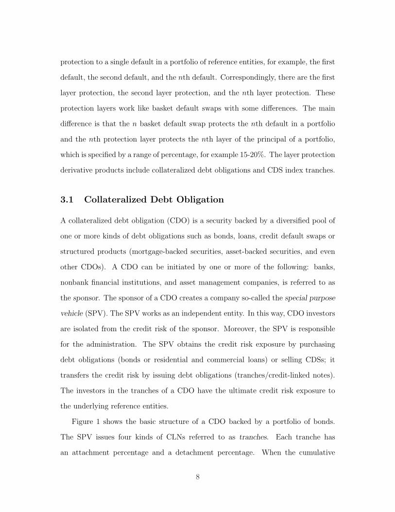
Figure 1 shows the basic structure of a CDO backed by a portfolio of bonds.

The SPV issues four kinds of CLNs referred to as tranches. Each tranche has

an attachment percentage and a detachment percentage. When the cumulative

8

percentage loss of the portfolio of bonds reaches the attachment percentage, investors

in the tranche start to lose their principal, and when the cumulative percentage loss

of principal reaches the detachment percentage, the investors in the tranche lose all

their principal and no further loss can occur to them. For example, in Figure 1 the

second tranche has an attachment percentage of 5% and a detachment percentage

of 15%. The tranche will be used to covered the cumulative loss during the life of

a CDO in excess of 5% (its attachment percentage) and up to a maximum of 15%

(its detachment percentage).

In the literature, tranches of a CDO are classified as subordinate/equity tranche,

mezzanine tranches, and senior tranches according to their subordinate levels.5 For

example, in Figure 1 tranche 1 is an equity tranche, tranches 2 and 3 are mezzanine

tranches, and tranche 4 is a senior tranche. Because the equity tranche is extremely

risky, the sponsor of a CDO holds the equity tranche and the SPV sells other tranches

to investors.

If the SPV of a CDO actually owns the underlying debt obligations, the CDO

is referred to as a cash CDO. Cash CDOs can be classified as collateralized bond

5See Lucas, Goodman, and Fabozzi (2006).

9

obligations (CBO) and collateralized loan obligation (CLO). The former have only

bonds in their pool of debt obligations, and the latter have only commercial loans

in their pool of debt obligations. If the SPV of a CDO does not own the debt

obligations, instead obtaining the credit risk exposure by selling CDSs on the debt

obligations of reference entities, the CDO is referred to as a synthetic CDO.

Based on the motivation of sponsors, CDOs can be classified as balance sheet

CDOs and arbitrage CDOs. The motivation of balance sheet CDOs (primarily

CLO) is to transfer the risk of loans in a sponsoring bank’s portfolio in order to

reduce regulatory capital requirements. The motivation of arbitrage CDOs is to

arbitrage the price difference between the underlying pool of debt obligations and

CDO tranches.

3.2 CDS index tranches

With the innovation of CDXs, the synthetic CDO technology is applied to slice CDXs

into standardized tranches with different subordinate levels to satisfy investors with

different risk favorites. The tranches of an index provide the layer protections to

the underlying portfolio risk in the same way as the tranches of a CDO as has been

explained earlier.

Both of the most actively traded indexes— the Dow Jones CDX NA IG and

the iTraxx Europe— are sliced into five tranches: equity tranche, junior mezzanine

tranche, senior mezzanine tranche, junior senior tranche, and super senior tranche.

The standard tranche structure of the Dow Jones CDX NA IG is 0-3%, 3-7%, 7-10%,

10-15%, and 15-30%. The standard tranche structure of the iTraxx Europe is 0-3%,

3-6%, 6-9%, 9-12%, and 12-22%.

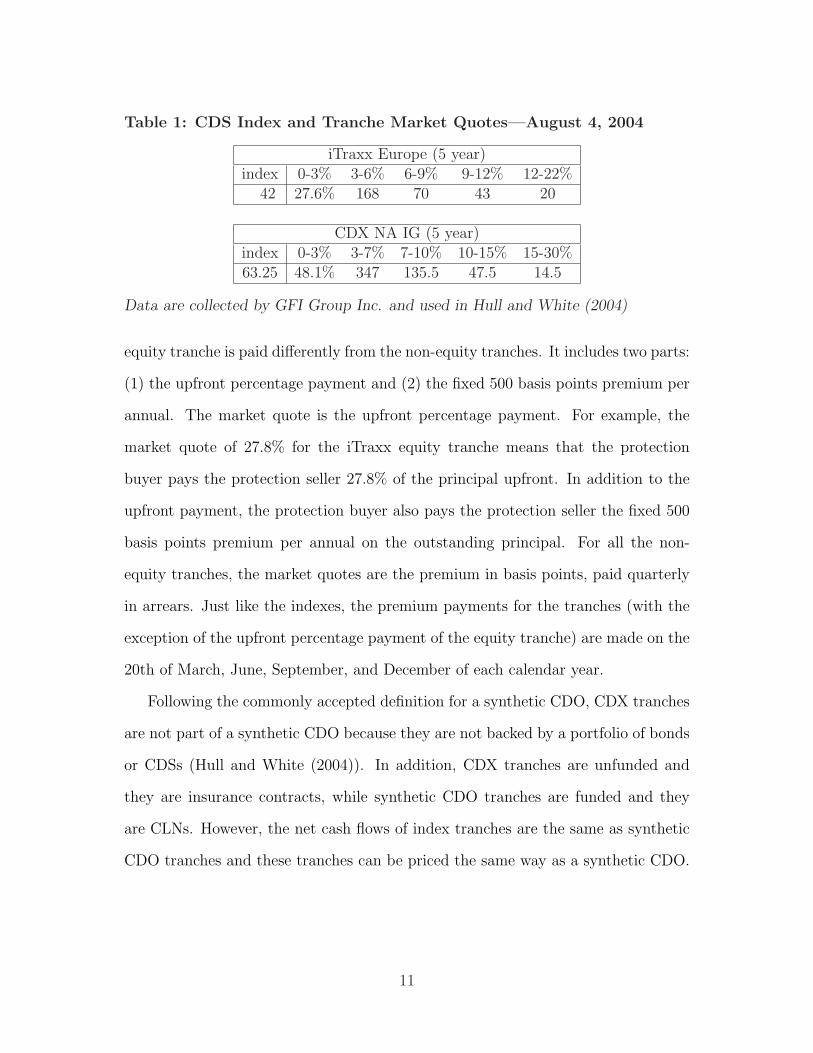
Table 1 shows the index and tranches market quotes for the CDX NA IG and

the iTraxx Europe on August 4, 2004. For both indexes, the swap premium of the

10

Table 1: CDS Index and Tranche Market Quotes—August 4, 2004

iTraxx Europe (5 year)index 0-3% 3-6% 6-9% 9-12% 12-22%

42 27.6% 168 70 43 20

CDX NA IG (5 year)index 0-3% 3-7% 7-10% 10-15% 15-30%63.25 48.1% 347 135.5 47.5 14.5

Data are collected by GFI Group Inc. and used in Hull and White (2004)

equity tranche is paid differently from the non-equity tranches. It includes two parts:

(1) the upfront percentage payment and (2) the fixed 500 basis points premium per

annual. The market quote is the upfront percentage payment. For example, the

market quote of 27.8% for the iTraxx equity tranche means that the protection

buyer pays the protection seller 27.8% of the principal upfront. In addition to the

upfront payment, the protection buyer also pays the protection seller the fixed 500

basis points premium per annual on the outstanding principal. For all the non-

equity tranches, the market quotes are the premium in basis points, paid quarterly

in arrears. Just like the indexes, the premium payments for the tranches (with the

exception of the upfront percentage payment of the equity tranche) are made on the

20th of March, June, September, and December of each calendar year.

Following the commonly accepted definition for a synthetic CDO, CDX tranches

are not part of a synthetic CDO because they are not backed by a portfolio of bonds

or CDSs (Hull and White (2004)). In addition, CDX tranches are unfunded and

they are insurance contracts, while synthetic CDO tranches are funded and they

are CLNs. However, the net cash flows of index tranches are the same as synthetic

CDO tranches and these tranches can be priced the same way as a synthetic CDO.

11

4 One-Factor Copula Model

The critical input into pricing a synthetic CDO and CDS index tranches is an esti-

mate of the default dependence (default correlation) between the underlying assets.

One popular method for estimating the dependence structure is using copula func-

tions, a method first applied in actuarial science. While there are several types of

copula function models, Li (1999, 2000) introduces the one-factor Gaussian copula

model for the case of two companies and Laurent and Gregory (2003) extend the

model to the case of N companies. Several extensions to the one-factor Gaussian

copula model are subsequently introduced into the literature. In this section, we

provide a general description of the one-factor copula function, introduce the market

standard model, and review both the one-factor double t copula model (Hull and

White (2004)) and the one-factor normal inversion Gaussian copula model (Kale-

manova, Schmid, and Werner (2005)).

Suppose that a CDO includes n assets i = 1, 2, . . . , n and the default times τi of

the ith asset follows a Poisson process with a parameter λi. The λi is the default

intensity of the ith asset. Then the probability of a default occurring before the

time t is

P (τi < t) = 1− exp(−λit). (1)

In a one-factor copula model, it is assumed that the default time τi for the ith

company is related to a random variable Xi with a zero mean and a unit variance.

For any given time t, there is a corresponding value x such that

P (Xi < x) = P (τi < t), i = 1, 2, . . . , n. (2)

Moreover, the one-factor copula model assumes that each random variable Xi is the

12

sum of two components

Xi = aiM +√

1− a2i Zi, i = 1, 2, . . . , n, (3)

where Zi is the idiosyncratic component of company i, and M is the common com-

ponent of the market. It is assumed that the M and Zi’s are mutually independent

random variables. For simplicity, it is also assumed that the random variables M

and Zi’s are identical. The factor ai satisfies −1 ≤ ai ≤ 1. The default correlation

between Xi and Xj is aiaj, (i 6= j).

Let F denote the cumulative distribution of the Zi’s and G denote the cumulative

distribution of the Xi’s. Then given the market condition M = m, we have

P (Zi < x|M = m) = F (x− aim√

1− a2i

), (4)

and the conditional default probability is

P (τi < t|M = m) = FG−1[P (τi < t)]− aim√1− a2

i

. (5)

For simplicity, the following two assumptions are made:

• All the companies have the same default intensity, i.e, λi = λ.

• The pairwise default correlations are the same, i.e, in equation (3), ai = a.

The second assumption means that the contribution of the market component is

the same for all the companies and the correlation between any two companies is

constant, β = a2.

Under these assumptions, given the market situation M = m, all the companies

have the same cumulative risk-neutral default probability Dt|m. Moreover, for a

13

given value of the market component M , the defaults are mutually independent for

all the underlying companies. Letting Nt|m be the total defaults that have occurred

by time t conditional on the market condition M = m, then Nt|m follows a binomial

distribution Bin(n,Dt|m), and

P (Nt|m = j) =n!

j!(n− j)!Dj

t|m(1−Dt|m)n−j, j = 0, 1, 2, . . . , n. (6)

The probability that there will be exactly j defaults by time t is

P (Nt = j) = EMP (Nt|m) =

∫ ∞

−∞P (Nt|m = j)fM(m)dm, (7)

where fM(m) is the probability density function (pdf) of the random variable M .

4.1 Market Standard Model

Li (1999, 2000) was the first to suggest that the Gaussian copula can be employed

in credit risk modeling to estimate the correlation default. In a one-factor Gaussian

copula model, the distributions of the common market component M and the indi-

vidual component Zi’s in equation (3) are standard normal Gaussian distributions.

Because the sum of two independent Gaussian distributions is still a Gaussian dis-

tribution, the Xi’s in equation (3) have a closed form. It can be verified that the

Xi’s have a standard normal distribution.

The one-factor copula Gaussian copula model is the market standard model when

implemented under the following assumptions:

• a fixed recovery rate of 40%,

• the same CDS spreads for all of the underlying reference entities,

• the same pairwise correlations,

14

• the same default intensities for all the underlying reference entities.

The market standard model does not appear to fit market data well (see Hull and

White (2004) and Kalemanova et al. (2005)). In practice, market practitioners use

implied correlations and base correlations.

The implied correlation for a CDO tranche is the correlation that makes the

value of a contract on the CDO tranche zero when pricing the CDO with the market

standard model. For a CDO tranche, when inputting its implied correlation into

the market standard model, the simulated price of the tranche should be its market

price.

McGinty, Beinstein, Ahluwalia, and Watts (2004) introduced base correlations

in CDO pricing. To understand base correlations, let’s use an example. Recalling

the CDX NA IG tranches 0-3%, 3-7%,7-10%, 10-15%, and 15%-30%, and assuming

there exists a sequence of equity tranches 0-3%, 0-7%, 0-10%, 0-15%, and 0-30%, the

premium payment on an equity tranche is a combination of the premium payment

of the CDX NA IG tranches that are included in the corresponding equity tranche.

For example, the equity tranche 0-10% includes three CDX NA IG tranches: 0-3%,

3-7%, and 7-10%. The premium payment on the equity tranche 0-10% includes

three parts. The part of 0-3% is paid the same way as the CDX NA IG tranche

0-3%, the part of 3-7% is paid the same way as the CDX NA IG tranche 3-7%, and

the part of 7-10% is paid the same way as the CDX NA IG tranche 7-10%. Then

the definition of base correlation is the correlation input that make the prices of the

contracts on these series of equity tranches zero. For example, the base correlation

for the CDX NA IG tranche 7-10% is the implied correlation that makes the price

of a contract on the equity tranche 0-10% zero.

15

4.2 One-Factor Double t Copula Model

The natural extension to a one-factor Gaussian copula model is using heavy-tailed

distributions. Hull and White (2004) propose a one-factor double t copula model.

In the model, the common market component M and the individual components Zi

in equation (3) are assumed to have a normalized Student’s t distribution

M =√

(nM − 2)/nMTnM, TnM

∼ T (nM)

Zi =√

(ni − 2)/niTni, Tni

∼ T (ni), (8)

where Tn is a Student’s t distribution with degrees of freedom n = 3, 4, 5, . . . .

In the model, the distributions of Xi’s do not have a closed form but instead

must be calculated numerically.

Hull and White (2004) find that the one-factor double t copula model fits market

prices well when using the Student’s t distribution with 4 degrees of freedom for M

and Zi’s.

4.3 One-Factor Normal Inverse Gaussian Copula Model

Kalemanova, Schmid, and Werner (2005) propose utilizing normal inverse Gaussian

distributions in a one-factor copula model. A normal inverse Gaussian distribution

is a mixture of normal and inverse Gaussian distributions.

An inverse Gaussian distribution has the following density function

fIG(x; ζ, η) =

ζ√2πη

x−3/2 exp(− (ζ−ηx)2

2ηx), if x > 0

0, if x ≤ 0, (9)

where ζ > 0 and η > 0 are two parameters. We denote the inverse Gaussian

distribution as IG(ζ, η).

16

Suppose Y is an inverse Gaussian distribution. A normal Gaussian distribution

X ∼ N (υ, σ2) is a normal inverse Gaussian (NIG) distribution when its mean υ and

variance σ2 are random variables as given below

υ = µ + βY, σ2 = Y

Y ∼ IG(δγ, γ2), (10)

where δ > 0, 0 ≤ |β| < α, and γ :=√

α2 − β2. The distribution of the random

variable X is denoted by X ∼ (α, β, µ, δ). The density of X is

f(x; α, β, µ, δ) =δα exp(δγ + β(x− u))

π√

δ2 + (x− µ)2K(α

√δ2 + (x− µ)2), (11)

where K(.) is the modified Bessel function of the third kind as defined below

K(ω) :=1

2

∫ ∞

0

exp(−1

2ω(t− t−1))dt. (12)

The mean and variance of the NIG distribution X are respectively

E(X) = µ +δβ

γ, V ar(X) =

δα2

γ3. (13)

The family of NIG distributions has two main properties. One is the closure

under the scale transition

X ∼ NIG(α, β, µ, δ) ⇒ cX ∼ NIG(α

c,β

c, cµ, cδ). (14)

The other is that if two independent NIG random variables X and Y have the same

α and β parameters, then the sum of these two variables is still an NIG variable as

17

shown below

X ∼ NIG(α, β, µ1, δ1), Y ∼ NIG(α, β, µ2, δ)

⇒ X + Y ∼ NIG(α, β, µ1 + µ2δ1 + δ2). (15)

When using NIG distributions in a one-factor copula model, the model is referred

to as a one-factor normal inverse Gaussian copula model. The distributions for M

and Zi’s in equation (3) are given below

M ∼ NIG(α, β,− αβ√α2 − β2

, α)

Zi ∼ NIG(α√

1− a2i

ai

,β√

1− a2i

ai

,− αβ√

1− a2i

ai

√α2 − β2

,α√

1− a2i

ai

).

(16)

The distributions of Xi’s in equation (3) are

Xi ∼ NIG(α

ai

,β

ai

,− αβ√

1− a2i

ai

√α2 − β2

,α

ai

). (17)

The selection of the parameters makes the variables Xi’s, M , and Zi’s have a zero

mean, and a unit variance when β = 0.

The one-factor normal inverse Gaussian copula model fits market data a little bit

better than the one-factor double t copula model. The advantage of the one-factor

normal inverse Gaussian copula model is that the Xi’s in the model have a closed

form. This makes the computing time is reduced significantly, compared with that

of the one-factor double t copula model. The former is about five times faster than

the latter.

18

5 Structural Model

Hull, Predescu, and White (2005) propose the structural model to price the default

correlation in tranches of a CDO or an index. The idea is based on Merton’s model

(1974) and its extension by Black and Cox (1976). It is assumed that the value of

a company follows a stochastic process, and if the value of the company goes below

a minimum value (barrier), the company defaults.

In the model, N different companies are assumed and the value of company

i (1 ≤ i ≤ N) at time t is denoted by Vi. The value of the company follows a

stochastic process as shown below

dVi = µiVidt + σiVidXi, (18)

where µi is the expected growth rate of the value of company i, σi is the volatility of

the value of company i, and Xi(t) is a variable following a continuous-time Gaussian

stochastic process (Wiener process). The barrier for company i is denoted by Bi.

Whenever the value of company i goes below the barrier Bi, it defaults.

Without the loss of generality, it is assumed that Xi(0) = 0. Applying Ito’s

formula to ln Vi, it is easy to show that

Xi(t) =ln Vi(t)− ln Vi(0)− (µi − σ2

i /2)

σi

. (19)

Corresponding to Bi, there is a barrier B∗i for the variable Xi as given below

B∗i =

ln Bi − ln Vi(0)− (µi − σ2i /2)t

σi

. (20)

19

When Xi falls below B∗i , company i defaults. Denote

βi =ln Hi − ln Vi(0)

σi

γi = −µi − σ2i /2

σi

, (21)

then B∗i = βi + γit.

To model the default correlation, it is assumed that each Wiener process Xi

follows a two-component process which includes a common Wiener process M and

an idiosyncratic Wiener process Zi. It is expressed as

dXi(t) = ai(t)dM(t) +√

1− a2i (t)dZi(t), (22)

where the variable ai, 1 ≤ ai ≤ 1 is used to control the weight of the two-component

process. The Wiener processes M and Zi’s are uncorrelated with each other. In this

model, the default correlation between two companies i and j is aiaj.

The model can be implemented by Monte Carlo simulation. Hull, Predescu, and

White (2005) implement the model in the three different ways:

• Base case: constant correlation and constant recovery rate.

• Stochastic Corr.: stochastic correlation and constant recovery rate.

• Stochastic RR: stochastic correlation and stochastic recovery rate.

Two comparisons between the base-case structural model and the one-factor

Gaussian copula model are provided. One is to calculate the joint default prob-

abilities of two companies by both models. The other is to simulate the iTraxx

Europe index tranche market quote by both models. In both cases, the results of

these models are very close when the same default time correlations are input, while

the one-factor Gaussian copula is a good approximation to the base-case structural

20

model, the structural model has two advantages: it is a dynamic model and it has

a clear economic rationale.

6 Loss Process Model

Loss process models for pricing correlation risk have been developed by Schonbucher

(2005), Sidenius et al. (2005), Di Graziano and Rogers(2005), and Bennani (2005).

Here we introduce the basic idea of the loss process model as discussed by Schonbucher.

We omit the mathematical details.

6.1 Model Setup

The model is set up in the probability space (Ω, (Ft)0≤t≤T , Q), where Q is a spot

martingale measure, (Ft)0≤t≤T is the filtration satisfying the common definitions,

and Ω is the sample space. Assume that there are N company names in a portfolio.

Each name has the same notional principal in the portfolio. Under the assumption

of a homogenous recovery rate for all the companies, all companies have identical

losses in default which is normalized to one. The cumulative default loss process is

defined by

Lt =N∑

k

1τk≤t, (23)

where τk is the default time of company k, and the default indicator 1τk≤t is 1 when

τk ≤ t and 0 when τk > t. The loss process is an N -bounded, integer-valued, non-

decreasing Markov chain. Under Q-measure, the probability distribution of L(T ) at

time t < T is denoted by the vector p(t, T ) := (p0(t, T ), . . . , pN(t, T ))′, where the

pi’s are conditional probabilities

pi(t, T ) := P [L(T ) = i|Ft], i = 0, 2, . . . , N, t ≤ T. (24)

21

The conditional probability pi(t, T ) is the implied probability of L(T ) = i, T ≥ t

given the information up to time t. p(t, .) is referred to as the loss distribution at

time t.

6.2 Static Loss Process

To price a CDO, it is necessary to determine an implied initial loss distribution

p(0, T ). The implied initial loss distribution can be found by solving the evolution

of the loss process L(t). As the loss process L(t) is an inhomogeneous Markov chain

in a finite state space with N + 1 states 0, 1, 2, . . . , N, its transition probabilities

are uniquely determined by its generator matrix.

Assuming that there is only one-step transition at any given time t, the generator

matrix of the loss process has the following form

A(t) =

−λ0(t) λ0(t) 0 . . . 0 0

0 −λ1(t) λ1(t) . . . 0 0

......

.... . .

......

0 0 0 . . . −λN−1(t) λN−1(t)

0 0 0 . . . 0 0

, (25)

where the λi(t)′s are the transition rates i = 0, 1, . . . , N − 1. The state N is an

absorbing state.

The probability transition matrix, defined by Pij(t, T ) := P [L(T ) = j|L(t) = i],

satisfies the following Kolmogorov equations

ddT

Pi,0(t, T ) = −λ0(T )Pi,0(t, T )

ddT

Pi,j(t, T ) = −λj(T )Pi,j(t, T ) + λj−1(T )Pi,j−1(t, T )

ddT

Pi,N(t, T ) = −λN−1(T )Pi,N−1(t, T )

, (26)

22

for all i, j = 0, 1, . . . , N and 0 ≤ t ≤ T . The initial conditions are Pi,j(t, t) = 1i=j.

The solution of the Kolmogorov equations in equation (26) is as given below

Pi,j(t, T ) =

0 for i > j

exp− ∫ T

tλi(t, s)ds for i = j

∫ T

tPi,j−1(t, s)λj−1e

− R Tt λj(t,u)duds for i < j

. (27)

The representation of the implied loss distribution at time t is simply

pi(t, T ) = P [L(T ) = i|Ft] = PL(t),i(t, T ). (28)

For example, if L(t) = k, then the implied loss distribution at time t is

pi(t, T ) = Pk,i(t, T ). (29)

6.3 Dynamic Loss Process

In the dynamics version of the loss process model, the loss process follows a Poisson

process with time- and state-dependent inhomogeneous default intensities λL(t)(t),

L(t) = 0, . . . , N − 1, which are the transition rates in the generator matrix in

equation (25). The aggregate default intensity λL(t)(t) can be expressed in terms of

the individual intensities λk(t)

λL(t)(t) =∑

k∈S(t)

λk(t), (30)

where S(t) := 1 ≤ k ≤ N |τk > t is the set of companies that have not defaulted

by time t.

The loss process is assumed to follow a Poisson process with stochastic intensity,

23

a process referred to as a Cox process.

dλi(t, T ) = µi(t, T )dT + σi(t, T )dB(t), i = 0, . . . , N − 1, (31)

where B(t) is a d-dimension Q-Brownian motion, the µi(t, T )’s are the drifts of

the stochastic processes, and the σi(t, T )’s are the d-dimension volatilities of the

stochastic processes. To keep the stochastic processes consistent with the loss process

L(t), the following conditions must be satisfied

PL(t),i(t, T )µi(t, T ) = σi(t, T )υL(t),i(t, T ), 0 ≤ i ≤ N − 1, t ≤ T, (32)

where, υn,m(t, T )’s are given by

υi,j =

0 for i > j

Pnm(t, T )− ∫ T

tσi(t, s)ds for i = j

∫ T

te−

R Ts λj(t,u)du[σPa

i,j−1(t, s)− Pij(t, s)σj(t, s)]ds for i < j

, (33)

with

σPai,j−1(t, T ) = Pi,j−1(t, T ) + λm−1(t, T )υn,m−1(t, T ). (34)

6.4 Default Correlation

In the loss process model, the default correlations between companies can arise from

both the transition rates of the loss process and the volatilities of the stochastic

processes. To understand the default dependence by the transition rates, recall the

concept of default correlation. The default correlation is the phenomenon of joint

defaults and a clustering of defaults. After one or more companies defaults, the

individual default intensities of the surviving companies increase. The dependence

24

of individual default intensities on the default number (loss process L(t)) can be

reflected by a proper selection of the transition rates λi(t), i = 0, 1, . . . , N − 1.

This is the way that the transition rates can cause the default dependence between

companies.

The default dependence by the volatilities can be explained by considering the

case of a one-dimension driving Brownian motion. For non-zero transition rate

volatilities

σi(t, T ) > 0 for all 0 ≤ i ≤ N − 1, (35)

Brownian motion works like an indicator of the common market condition. If its

value is positive, the market condition is bad and all the transition rates are larger;

if its value is negative, the market condition is good and all the transition rates are

smaller.

6.5 Implementation of Dynamic Loss Process Model

The model can be implemented by a Monte Carlo method. For pricing a CDO with

a maturity T , the procedure is as follows:

1. Initial condition: t = 0, L(0) = 0 (p0(0, 0) = 1), and specify λi(0, 0)’s and

σi(0, .)’s.

2. Simulate a Brownian motion trial.

3. s → s + ∆s: (until s = T )

• Calculate P0,m(0, s) from equation (27), and υ0,j(0, s) from equation (33),

and use them and σi(0, s) to calculate µi(0, s) from equation (32).

• Calculate λi(0, s + ∆s) using the Euler scheme and µi(0,s)S and σi(0, s).

25

• In a Euler scheme, calculate the loss distribution pi(0, s + ∆s) from (27)

and using the representation of the loss distribution in equation (29).

• The loss distribution pi(0, .) on the time period of (0, T ) is then calculated.

4. Repeat steps 2-4 until the average loss distributions pi(0, .) of all the trials

converge.

5. Using the average loss distributions pi(0, .) to price a CDO.

The loss process model can also be used to price other portfolio credit derivatives

such as basket default swaps, options on CDS indexes, and options on CDS indexes

tranches.

7 Models for Pricing Correlation Risk

In this section, we give our suggestions for future research. It includes two parts. In

the first part, we analyze the shortcoming of the one-factor double t copula model,

and then propose four new heavy-tailed one-factor copula models. In the second

part, we give our proposal for improving the structural model and the loss process

model.

7.1 Heavy-Tailed Copula Models

Hull and White (2004) first use heavy-tailed distributions (Student’s t distributions)

in a one-factor copula model. In their so-called one-factor double t copula model,

the degrees of freedom parameter of t distribution ν decreases, the tail-fatness of

copula function increases, when the degrees of freedom parameter ν goes to infinity,

the model becomes the one-factor Gaussian copula model.

26

As mentioned before, Hull and White find that the double t copula model fits

market data well when the degrees of freedom parameter ν is equal to 4. But the

simulation by Kalemanova et al. (2005) shows a different result. When Kalemanova

et al. compare their model with the double t copula model, in addition to the

simulation results by their own model, they also give the simulation results by the

double t copula model for both the cases of the degrees of freedom parameter ν

equal to 3 and 4. These simulation results show that the double t copula model fits

market data better when ν = 3 than ν = 4. One difference in these two works is that

different market data are used in the simulation. Hull and White use market data

for the 5-year iTraxx Europe tranches on August 4, 2004, while Kalemanova et al.

use market data on April 12, 2006. Therefore, the difference, related to how many

degrees of freedom make the double t copula fit market data well, may suggest

that for market data in different times, the double t copula model with different

tail-fatnesses works well.

The drawbacks of the double t copula are that its tail fatness cannot be changed

continuously and the maximum tail-fatness occurs when the degrees of freedom

parameter ν equal to 3. In order to fit market data well over time, it is necessary

that the tail-fatness of a one-factor copula model can be adjusted continuously and

can be much larger than the maximum tail-fatness of the one-factor double t copula

model.

In the following, we suggest four one-factor heavy-tailed copula models. Each

model has (1) a tail-fatness parameter that can be changed continuously and (2)

a maximum tail-fatness much larger than that of the one-factor double t copula

model.

27

7.1.1 One-factor double mixture Gaussian copula model

The mixture Gaussian distribution is a mixture distribution of two or more Gaussian

distributions. For simplicity, we consider the case of the mixture distribution of two

Gaussian distributions which have a zero mean. If the random variable Y is such a

mixture Gaussian distribution, then it can be expressed as

Y =

X1 with probability p

X2 with probability 1− p, (36)

where X1 and X2 are independent normal Gaussian distributions with a zero mean

EX1 = EX2 = 0, V arX1 = σ21 and V arX2 = σ2

2, (37)

with σ1 > σ2. The mixture Gaussian distribution Y has a zero mean. Its variance

is

V arY = pσ21 + (1− p)σ2

2. (38)

The pdf of the distribution Y is

fY (y) =p√

2πσ1

exp(− y2

2σ21

) +1− p√2πσ2

exp(− y2

2σ22

). (39)

The mixture Gaussian distribution Y can be normalized by the following transition

Y =1√

σ21 + σ2

2

Y. (40)

The pdf of Y is

fY (y) =p√

pσ21+(1−p)σ2

2√2πσ1

exp(−y2(pσ21+(1−p)σ2

2)

2σ21

)

+(1−p)

√pσ2

1+(1−p)σ22√

2πσ2exp(−y2(pσ2

1+(1−p)σ22)

2σ22

). (41)

28

Using the standardized mixture Gaussian distribution in equation (41) as the

distribution of the M and Zi’s in equation (3), we obtain our first extension to the

one-factor Gaussian copula model which we refer to as a double mixture Gaussian

distribution copula model. In this model, the tail-fatness of the M and Z’s is de-

termined by the parameters σ1, σ2, and p. In the implementation of the model, we

can fix the parameters σ1 and σ2, and make the parameter p the only parameter to

control the tail-fatness of the copula function.

7.1.2 One-factor double t distribution with fractional degrees of freedom

copula model

The pdf of the gamma(α, β) distribution is

f(x|α, β) =1

Γ(α)βαxα−1exp(−x/β), 0 < x < ∞, α > 0, β > 0 (42)

Setting α = ν/2 and β = 2, we obtain an important special case of the gamma

distribution, the Chi-square distribution, which has the following pdf:

f(x|ν) =1

Γ(ν/2)2ν/2xν−1exp(−x/2), 0 < x < ∞, ν > 0. (43)

If the degrees of freedom parameter ν is an integer, equation (43) is the Chi-square

distribution with ν degrees of freedom. However, the degrees of freedom parameter

ν need not be an integer. When ν is extended to a positive real number, we get the

Chi-square distribution with ν fractional degrees of freedom.

If U is a standard normal distribution, V is a Chi-square distribution with ν

fractional degrees of freedom, and U and V are independent, then T = U/√

V/ν

29

has the following pdf

fT (t|ν) =Γ(ν+1

2)

Γ(ν2)√

νπ(1 + t2/ν)−(ν+1)/2, 0 < x < ∞, ν > 0. (44)

This is the Student’s t distribution with ν fractional degrees of freedom (see Mardia

and Zemroch (1978)). Its mean and variance are respectively

ET = 0, ν > 1; V arT =ν

ν − 2, ν > 2. (45)

For ν > 2, the Student’s t distribution in equation (44) can be normalized by making

the transition

X =√

(ν − 2)/νT, ν > 2. (46)

The normalized Student’s t distribution with ν(ν > 2) factional degrees of freedom

has the following pdf

fX(x|ν) =

√ν

ν − 2

Γ(ν+12

)

Γ(ν2)√

νπ(1 +

x2

ν − 2)−(ν+1)/2, 0 < x < ∞, ν > 2. (47)

Using the normalized Student’s t distribution with factional degrees of freedom

as the distribution of the M and Zi’s in equation (3), we get our second extension

to the one-factor Gaussian copula model which we refer to as a double t distribution

with fractional degrees of freedom copula model. In this model, the tail-fatness of

the M and Zi’s can be changed continuously by adjusting the fractional degrees of

freedom parameter ν.

30

7.1.3 One-factor double mixture distribution of t and Gaussian distri-

bution copula model

In the previous model, the tail fatness of the M and Zi’s is controlled by the frac-

tional degrees of freedom parameter of the Student’s t distribution. Here, we in-

troduce another distribution function for the M and Zi’s, the mixture distribution

of the Student’s t and the Gaussian distributions. Assume U is a normalized Stu-

dent’s t distribution with fractional degrees of freedom, and V is a standard normal

distribution. We can express a mixture distribution X as

X =

U with probability 1− p

V with probability p, 0 ≤ p ≤ 1, (48)

where p is the proportion of the Gaussian component in the mixture distribution

X. The pdf of the X is

f(x) = p√2π

exp(−x2/2)+

+(1− p)√

ν−2ν

Γ( ν+12

)√νπΓ(ν/2)

(1 + x2

ν−2)−(ν+1)/2

, (49)

where ν is the fractional degrees of freedom of the Student’s t distribution.

Using the mixture distribution of Student’s t and Gaussian distributions in equa-

tion (3) as the distribution of the M and Zi’s, we get our third extension to the

one-factor Gaussian copula model which we refer to as a double mixture distribution

of Student’s t and Gaussian distribution copula model. In this model, the tail-fatness

of the M and Z’s is controlled by the parameter p when the parameter ν is fixed.

31

7.1.4 One-factor double smoothly truncated stable copula model

In this part, we first introduce the stable distribution and the smoothly truncated

stable distribution, and then provide our proposed model.

Stable distribution

A non-trivial distribution g is a stable distribution if and only if for a sequence of

independent, identical random variables Xi,, i = 1, 2, 3, . . . , n with a distribution g,

the constants cn > 0 and dn can always be found for any n > 1 such that

cn(X1 + X2 + · · ·+ Xn) + dnd= X1.

In general, a stable distribution cannot be expressed in a closed form except

for three special cases: Gaussian, Gauchy, and Levy distributions. However, the

characteristic function always exists and can be expressed in a closed form. For a

random variable X with a stable distribution g, the characteristic function of the X

can be expressed in the following form

φX(t) = E exp(itX) =

exp(−γα|t|α[1− iβsign(t) tan(πα2

)] + iδt), α 6= 1

exp(−γ|t|[1 + iβ 2πsign(t) ln(|t|)] + iδt), α = 1

,

(50)

where 0 < α ≤ 2, γ ≥ 0, −1 ≤ β ≤ 1, and −∞ ≤ δ ≤ ∞, and the function of

sign(t) is 1 when t > 0, 0 when t = 0, and −1 when t < 0.

There are four characteristic parameters to describe a stable distribution. They

are: (1) the index of stability or the shape parameter α, (2) the scale parameter γ,

(3) the skewness parameter β, and (4) the location parameter δ. A stable distribu-

tion g is called the α stable distribution and is denoted Sα(δ, β, σ) = S(α, σ, β, δ).

The family of α stable distributions has three attractive properties:

32

• The sum of independent α stable distributions is still an α stable distribution,

a property is referred to as stability.

• α stable distributions can be skewed.

• Compared with the normal distribution, α stable distributions can have a

fatter tail and a high peak around its center, a property which is referred to

as leptokurtosis.

Real world financial market data indicate that assets returns tend to be fat-

tailed, skewed, and perked around center. For this reason α stable distributions

have been a popular choice in modeling asset returns.6

Smoothly truncated α stable distribution

One inconvenience of a stable distribution is that it has an infinite variance except

in the case of α = 2. A new class of heavily-tailed functions is proposed by Menn

and Rachev (2005): smoothly truncated α stable distribution.

A smoothly truncated α stable distribution is an α stable distribution with its

two tails replaced by the tails of Gaussian distribution. The pdf can be expressed

as

f(x) =

h1(x) for x < a

gθ(x) for a ≤ δ ≤ b

h2(x) for x > b

, (51)

where hi(x), i = 1, 2 are the pdf of two normal distributions with means µi and stan-

dard deviations σi, and gθ(x) is the pdf of an α stable distribution with its parameter

vector θ = (α, γ, β, δ). To secure a well-defined smooth probability distribution, the

6see Rachev, Menn, and Fabozzi (2005).

33

following regularities are imposed:

h1(a) = gθ(a), h2(b) = gθ(b)

p1 :=∫ a

−∞ h1(x)dx =∫ a

−∞ gθ(x)dx

p2 :=∫∞

ah2(x)dx =

∫∞b

gθ(x)dx

σ1 = ψ(ϕ−1(p1))gθ(a)

, µ1 = a− σ1ϕ−1(p1)

σ2 = ψ(ϕ−1(p2))gθ(b)

, µ2 = b + σ2ϕ−1(p2)

, (52)

where ψ and ϕ denote the density and distribution functions of the standard normal

distribution, respectively. A smoothly truncated α stable distribution is referred to

as an STS-distribution and denoted by S[a,b]α (γ, β, δ). The probabilities p1 and p2

are referred to as the cut-off probabilities. The real numbers a and b are referred to

as the cut-off points.

The family of STS-distributions has two important properties. The first is that it

is closed under the scale and location transitions. This means that if the distribution

X is an STS-distribution, then for c, d ∈ R, the distribution Y := cX +d is an STS-

distribution. If X follows S[a,b]α (γ, β, δ), then Y follows S

[a,b]α (γ, β, δ) with

a = ca + d, b = cb + d, α = α,

γ = |c|γ, β = sign(c)β, δ =

cδ + d α = 1

cδ − 2πc log |c|σβ + d α 6= 1

,(53)

The other important property of the STS-distribution is that with respect to

an α stable distribution Sα(γ, β, δ), there is a unique normalized STS-distribution

S[a,b]α (γ, β, δ) whose cut-off points a and b are uniquely determined by the four pa-

rameters α, γ, β, and δ. Because of the uniqueness of cut-off points, the normalized

STS-distribution can be denoted by the NSTS-distribution Sα(γ, β, δ).

34

One-factor double smoothly truncated stable copula model

In the one-factor copula model given in equation (3), using the NSTS-distribution

Sα(γ, β, δ) for the distribution of the market component M and the individual com-

ponents Zi’s, we obtain the fourth extension to the one-factor Gaussian copula

model. We refer to the model as a one-factor double smoothly truncated α stable

copula model. In the model, we can fix the parameters γ, β, and δ, and make the

parameter α the only parameter to control the tail fatness of the copula function.

When the parameter α = 2, the model becomes the one-factor Gaussian copula

model. When α decreases, the tail-fatness increases.

7.2 Suggestions for Structural Model and Loss Process Model

The base-case structural model suggested by Hull et. al (2005) can be an alternative

method to the one-factor Gaussian copula model. The results of the two models are

close. Consider the fact that the one-factor double t copula model fits market data

much better than the one-factor Gaussian copula model according to Hull and White

(2004). A natural way to enhance the structural model is by applying heavy-tailed

distributions.

Unlike the one-factor copula model, where any continuous distribution with a

zero mean and a unit variance can be used, in the structural model there is a strong

constraint imposed on the distribution of the underlying stochastic processes. The

distribution for the common driving process M(t) and the individual driving process

Zi’s in equation (22) must satisfy a property of closure under summation. This

means that if two independent random variables follow a given distribution, then

the sum of these two variables still follow the same distribution. As explained earlier,

the α stable distribution has this property and has been used in financial modeling.7

7see Rachev and Mitnik (2000).

35

We suggest using the α stable distribution in the structural model.

The non-Gaussian α stable distribution has a drawback. Its variance does not

exist. The STS distribution is a good candidate to overcome this problem. For a STS

distribution, if the two cut-off points a and b are far away from the peak, the STS

distribution is approximately closed under summation. Based on this, employing the

STS distribution in the structural model should be the subject of future research.

In the dynamic loss process model, the default intensities λi’s follow stochastic

processes as shown in equation (31). It also a possible research direction to use the

α stable distribution and the STS distribution for the driving processes.

8 Summary

In this paper, we review three models for pricing portfolio risk: the one-factor

copula model, the structural model, and the loss process model. We then propose

how to improve these models by using heavy-tailed functions. For the one-factor

copula model, we suggest using (1) a double mixture Gaussian copula, (2) a double

t distribution with fractional copula, (3) a double mixture distribution of t and

Gaussian distributions copula, and (4) a double smoothly truncated α stable copula.

In each of these four new extensions to the one-factor Gaussian copula model, one

parameter is introduced to control the tail-fatness of the copula function. To improve

the structural and loss process models, we suggest using the stable distribution and

the smoothly truncated stable distribution for the underlying stochastic driving

processes.

36

References

[1] Amato J, Gyntelberg J (2005) CDS index tranches and the pricing of credit

risk correlations. BIS Quarterly Review, March 2005, pp 73-87

[2] Bennani N (2005) The forward loss model: a dynamic term struture approach

for the pricing of porftolio credit derivatives. Working paper, available at

http://www.defaultrisk.com/pp crdrv 95.htm

[3] Black F, Cox J (1976) Valuing corporate securities: some effects of bond inden-

ture provision. The Journal of Finance, vol 31, pp 351-367

[4] Di Graziano G, Rogers C (2005) A new approach to the modeling

and pricing of correlation credit derivatives. Working paper, available at

www.defaultrisk.com/pp crdrv 88.htm

[5] Duffie D (2004) Comments: irresistible reasons for better models of credit risk.

Financial Times, April 16, 2004

[6] Hull J, White A (2004) Valuation of a CDO and nth to default CDS without

monte carlo simulation. The Journal of Derivatives, vol 2, pp 8-23

[7] Hull J, Predescu M, White A (2005) The valuation of correlation-

dependent credit derivatives using a structural model. Working Paper, Joseph

L. Rotman School of Management, University of Toronto, available at

http://www.defaultrisk.com/pp crdrv 68.htm

[8] Kalemanova A, Schmid B, Werner R (2005) The normal inverse gaus-

sian distribution for synthetic CDO pricing. Working paper, available at

http://www.defaultrisk.com/pp crdrv 91.htm

37

[9] Laurent JP, Gregory J (2003) Basket default swaps, CDOs and factor copu-

las. Working paper, ISFA Actuarial School, University of Lyon, available at

http://www.defaultrisk.com/pp crdrv 26.htm

[10] Li DX (1999) The valuation of basket credit derivatives. CreditMetrics Monitor,

April 1999, pp 34-50

[11] Li DX (2000) On default correlation: a copula function approach. The Journal

of Fixed Income, vol 9, pp 43-54

[12] Lucas DJ, Goodman LS, Fabozzi FJ (2006) Collateralized debt obligations:

structures and analysis, 2nd edn. Wiley Finance, Hoboken, New Jersey

[13] Mardia K, Zemroch P (1978) Tables of the F- and related distributions with

algorithms. Academic Press, New York

[14] McGinty L, Beinstein E, Ahluwalia R, Watts M (2004) Credit correlation: a

guide. Credit Derivatives Strategy, JP Morgan, London, March 12, 2004

[15] Menn C, Rachev S (2005) A GARCH option pricing model with alpha-stable

innovations. European Journal of Operational Research, vol 163, pp 201-209

[16] Menn C, Rachev S (2005) Smoothly truncated stable distribu-

tions, Garch-models, and option pricing. Working paper, Univer-

sity of Karlsruhe and UCSB, available at http://www.statistik.uni-

karlsruhe.de/download/tr smoothly truncated.pdf

[17] Merton R (1974) On the pricing of corporate debt: the risk structure of interest

rates. The Journal of Finance, vol 29, pp 449-470

[18] Rachev S, Mitnik S (2000) Stable paretian models in finance. John Wiley, Series

in Financial Ecomomics and Quatitative Analysis, Chichester.

38

[19] Rachev S, Menn C, Fabozzi FJ (2005) Fat-tailed and skewed asset return dis-

tributions: implications for risk management, Portfolio selection, and Option

Pricing. Wiley Finance, Hoboken, New Jersey.

[20] Schonbucher P (2005) Portfolio losses and the term structure of loss transition

rates: a new methodology for the pricing of portfolio credit derivatives. Working

paper, available at http://www.defaultrisk.com/pp model 74.htm

[21] Sidenius J, Piterbarg V, Andersen L (2005) A new framework for

dynamic credit portfolio loss modeling. Working paper, available at

http://www.defaultrisk.com/pp model 83.htm

39