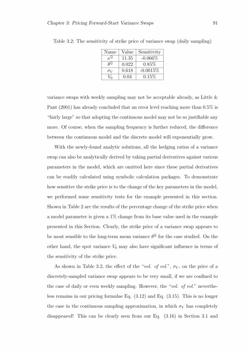
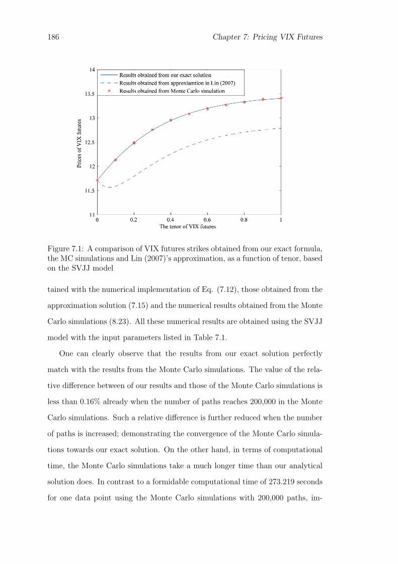
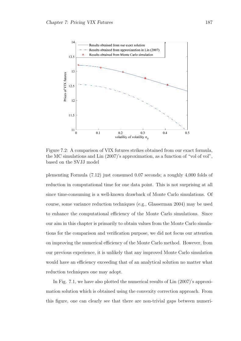
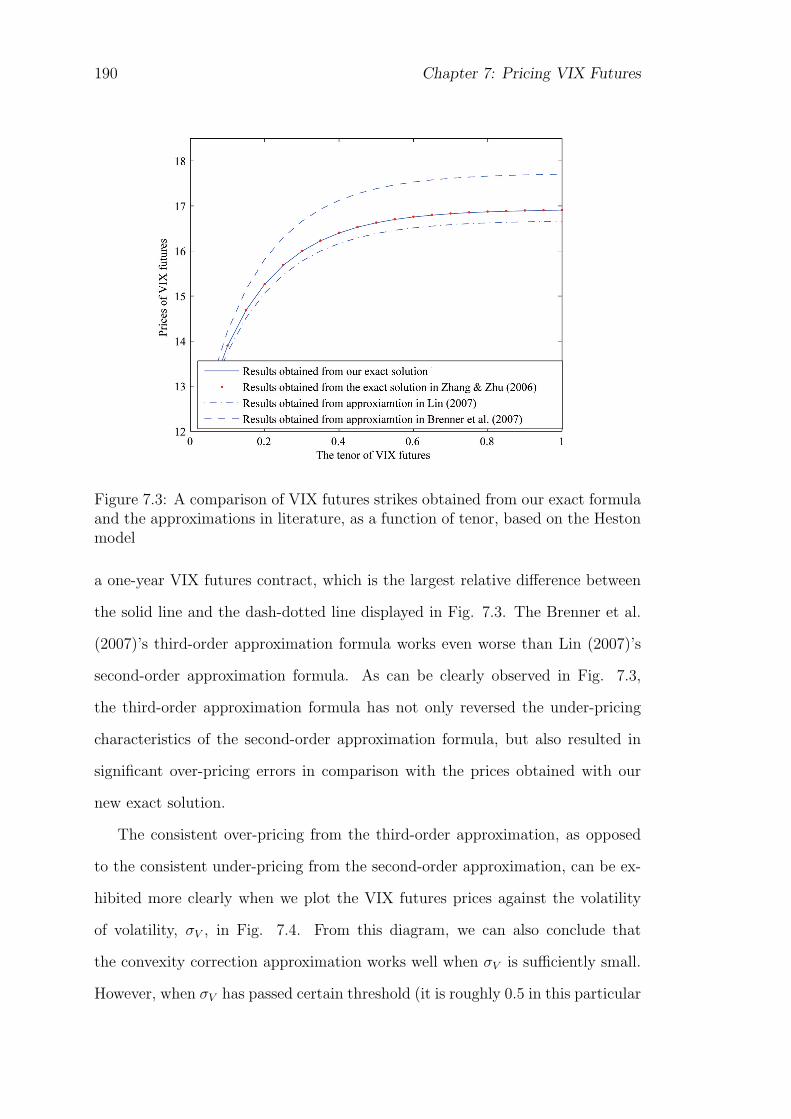
University of Wollongong Thesis Collections University of Wollongong Thesis Collection University of Wollongong Year Pricing volatility derivatives with stochastic volatility Guanghua Lian University of Wollongong Lian, Guanghua, Pricing volatility derivatives with stochastic volatility, Doctor of Phi- losophy thesis, School of Mathematics and Applied Statistics, Faculty of Informatics, University of Wollongong, 2010. http://ro.uow.edu.au/theses/3137 This paper is posted at Research Online.
Transcript
University of Wollongong Thesis Collections
University of Wollongong Thesis Collection
University of Wollongong Year
Pricing volatility derivatives with
stochastic volatility
Guanghua LianUniversity of Wollongong
Lian, Guanghua, Pricing volatility derivatives with stochastic volatility, Doctor of Phi-losophy thesis, School of Mathematics and Applied Statistics, Faculty of Informatics,University of Wollongong, 2010. http://ro.uow.edu.au/theses/3137
This paper is posted at Research Online.
Pricing Volatility Derivatives
with Stochastic Volatility
A thesis submitted in fulfillment of the
requirements for the award of the degree of
Doctor of Philosophy
from
University of Wollongong
by
Guanghua Lian, B.Sc. (Sichuan University)
M.A. (Huazhong University of Science and Technology)
School of Mathematics and Applied Statistics
2010
CERTIFICATION
I, Guanghua Lian, declare that this thesis, submitted in fulfilment of the require-
ments for the award of Doctor of Philosophy, in the School of Mathematics and
Applied Statistics, University of Wollongong, is wholly my own work unless oth-
erwise referenced or acknowledged. The document has not been submitted for
qualifications at any other academic institution.
Guanghua Lian
March, 2010
Acknowledgements
I would like to express my sincerest gratitude and appreciation to my super-
visor, Professor Song-Ping Zhu, for his insightful guidance and substantial advice
throughout the research. I, in particular, appreciate him for introducing me into
this wonderful research area and inspiring my numerous research ideas. His high
professional standard and rigorous attitude towards research have greatly influ-
enced me and become my principle that I will abide by in all of my life. It is he
who transformed me from a raw beginner into an active researcher, which fulfills
my dream of pursuing research in mathematical finance.
Also, I am especially grateful to Dr. Xiao-Ping Lu for her constant encour-
agements and warm care to me during my study. Without her help this thesis
could not have reached its present form. I wish to thank all the fellow friends in
the Center of Financial Mathematics and the School of Mathematics and Applied
Statistics in University of Wollongong, particularly Professor Matt Wand and Dr.
Pam Davy, who taught me statistics and Markov Chain Monte Carlo method,
Professor Timothy Marchant and Dr. Mark Nelson for their encouragement to
me and valuable advice for my research and career development. I trust that all
other people whom I have not specifically mentioned here are aware of my deep
appreciation.
Finally, the financial support from the University of Wollongong with HDR
tuition scholarship and University Postgraduate Research Award is also gratefully
acknowledged. I thank my parents and family for their years of dedication and
support to me and for their sincere concern about my life.
i
Abstract
Volatility derivatives are products where the volatility is the main underlying
notion. These products are particularly important for market investors as they
use them to have insight into the level of volatility to efficiently manage the market
volatility risk. This thesis makes a contribution to literature by presenting a set
of closed-form exact solutions for the pricing of volatility derivatives.
The first issue is the pricing of variance swaps, which is discussed in Chapter
2, 3, and 4. We first present an approach to solve the partial differential equation
(PDE), based on the Heston (1993) two-factor stochastic volatility, to obtain
closed-form exact solutions to price variance swaps with discrete sampling times.
We then extend our approach to price forward-start variance swaps to obtain
closed-form exact solutions. Finally, our approach is extended to price discretely-
sampled variance by further including random jumps in the return and volatility
processes. We show that our solutions can substantially improve the pricing
accuracy in comparison with those approximations in literature. Our approach is
also very versatile in terms of treating the pricing problem of variance swaps with
different definitions of discretely-sampled realized variance in a highly unified
way.
The second issue, which is covered in Chapter 5, and 6, is the pricing method
for volatility swaps. Papers focusing on analytically pricing discretely-sampled
volatility swaps are rare in literature, mainly due to the inherent difficulty as-
sociated with the nonlinearity in the pay-off function. We present a closed-form
exact solution for the pricing of discretely-sampled volatility swaps, under the
framework of Heston (1993) stochastic volatility model, based on the definition
of the so-called average of realized volatility. Our closed-form exact solution
for discretely-sampled volatility swaps can significantly reduce the computational
time in obtaining numerical values for the discretely-sampled volatility swaps, and
substantially improve the computational accuracy of discretely-sampled volatility
swaps, comparing with the continuous sampling approximation. We also investi-
gate the accuracy of the well-known convexity correction approximation in pric-
ing volatility swaps. Through both theoretical analysis and numerical examples,
ii
we show that the convexity correction approximation would result in significantly
large errors on some specifical parameters. The validity condition of the convexity
correction approximation and a new improved approximation are also presented.
The last issue, which is covered in Chapter 7 and 8, is the pricing of VIX
futures and options. We derive closed-form exact solutions for the fair value of
VIX futures and VIX options, under stochastic volatility model with simultane-
ous jumps in the asset price and volatility processes. As for the pricing of VIX
futures, we show that our exact solution can substantially improve the pricing
accuracy in comparison with the approximation in literature. We then demon-
strate how to estimate model parameters, using the Markov Chain Monte Carlo
(MCMC) method to analyze a set of coupled VIX and S&P500 data. We also con-
duct empirical studies to examine the performance of the four different stochastic
volatility models with or without jumps. Our empirical studies show that the
Heston stochastic volatility model can well capture the dynamics of S&P500 al-
ready and is a good candidate for the pricing of VIX futures. Incorporating jumps
into the underlying price can indeed further improve the pricing the VIX futures.
However, jumps added in the volatility process appear to add little improvement
for pricing VIX futures. As for the pricing of VIX options, we point out the solu-
tion procedure of Lin & Chang (2009)’s pricing formula for VIX options is wrong,
and alert the research community that this formula should not be further used.
More importantly, we present a new closed-form pricing formula for VIX options
and demonstrate its high efficiency in computing the numerical values of the price
of a VIX option. The numerical examples show that results obtained from our
formula consistently match up with those obtained from Monte Carlo simula-
tion perfectly, verifying the correctness of our formula; while the results obtained
from Lin & Chang (2009)’s pricing formula significantly differ from those from
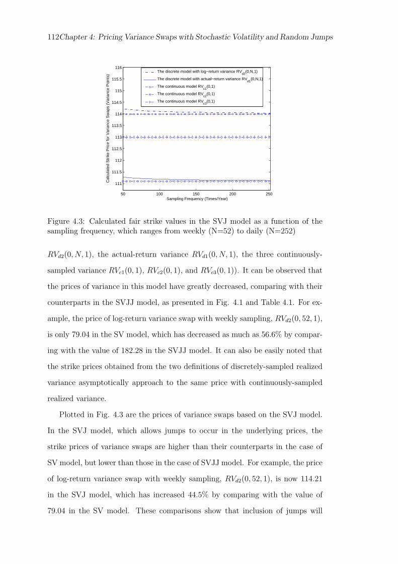
Monte Carlo simulation. Some other important and distinct properties of the
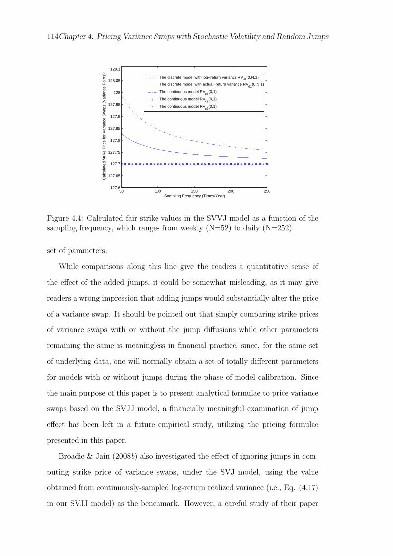
VIX options (e.g., put-call parity, the hedging ratios) have also been discussed.
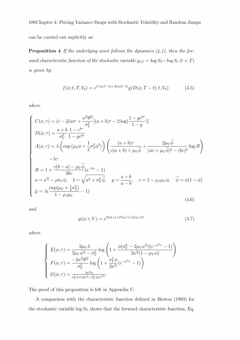
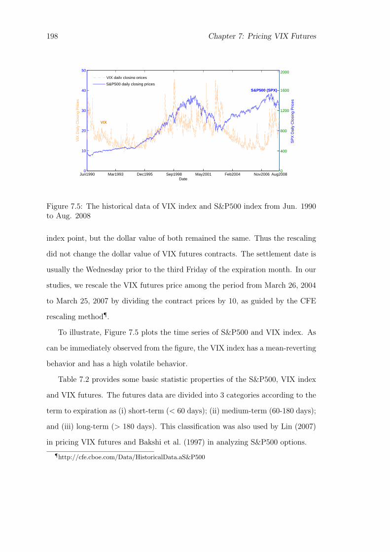
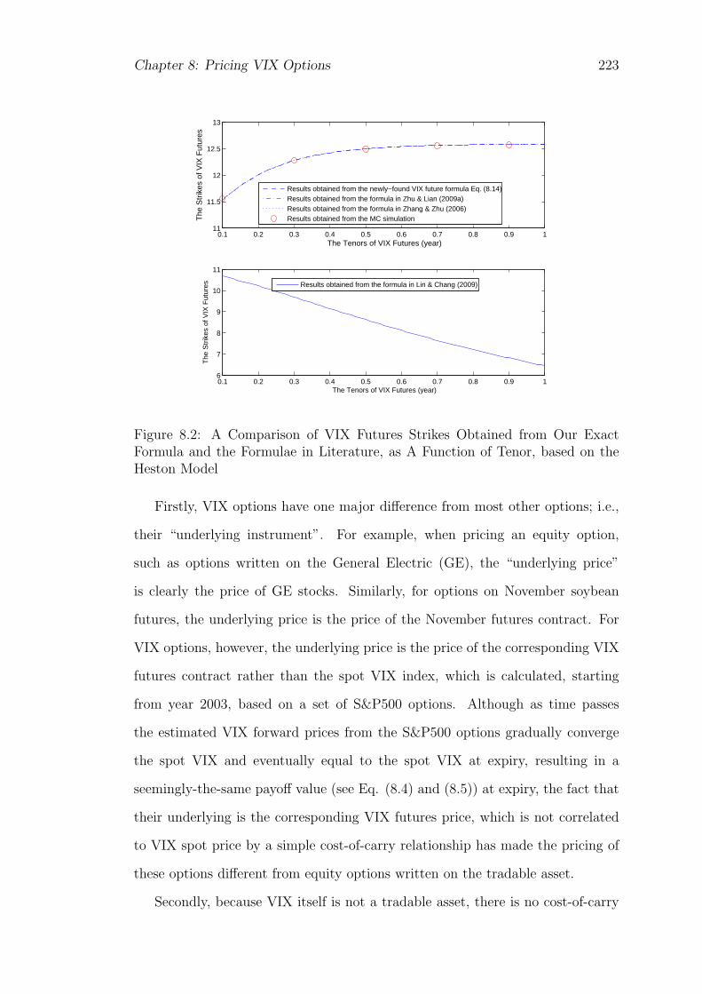
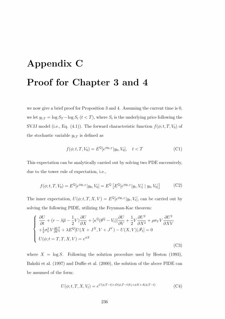
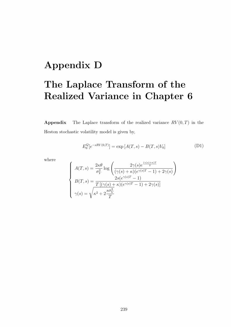
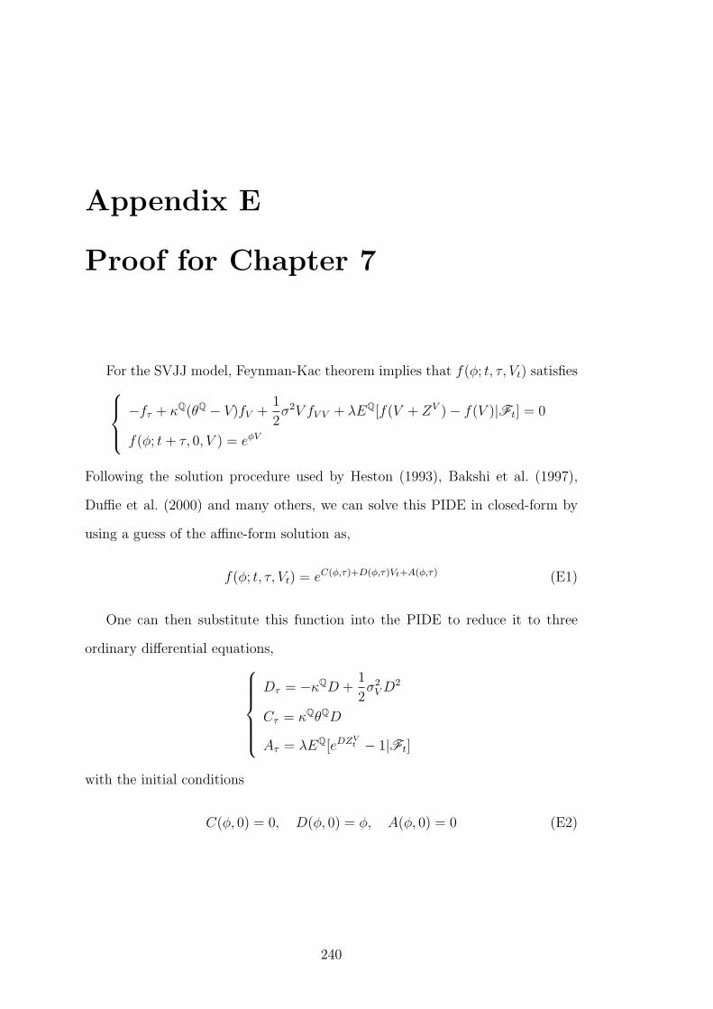
where St− is the value of the process St just before jump J occurs.
1.2.3 Connections Between PDE and SDE
The Feynman-Kac theorem and Kolmogoroff (Fokker-Plank) backward equations
are our key tool to study the pricing problem from the P(I)DE standpoint, by
relating the expectation of the derivative payoff under the martingale measure Q
with the P(I)DE, which can be solved analytically or numerically.
In general, the backward Kolmogoroff equation is applied by valuing derivative
securities, which might also include some optionality features, such as American
options which can be exercised by the holder at any time up to maturity time T .
For option pricing purposes we state this important result relating expectations
with respect to realizations of stochastic processes to specific PIDE-s.
14 Chapter 1: Introduction and Background
Theorem 4 (Kolmogoro Backward Equation and Feynman-Kac Theorem)
If µ(t, S) and σ2(t, S) satisfy the Lipschitz condition Eq. (1.13) and f(t, y) ∈
C2([0,∞)×R) satisfies the following partial integro-differential equations (PIDE)
∂f
∂t+ µ(t, S)
∂f
∂S+
1
2σ2(t, S)
∂2f
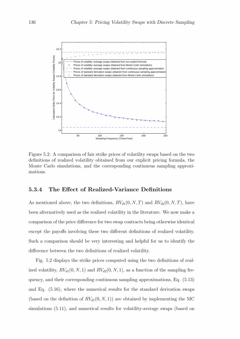
∂S2− g(t, S)f(t, S)
+γ(t, S)
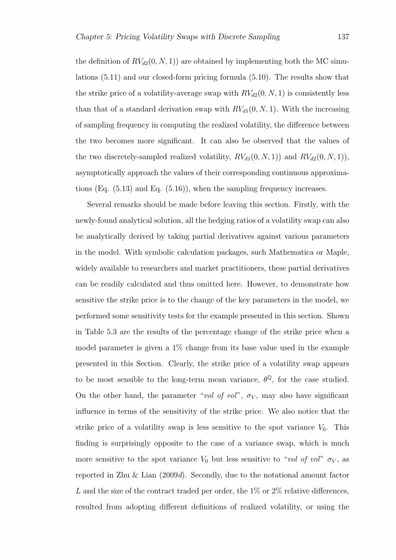
∫ ∞
−∞[f(t, S + j(t, S, J))− f(t, S)]ω(J)dJ = 0
(1.15)
with final condition f(T, S) = p(S), then the solution f(t, S) to the above PIDE
has the stochastic expectation representation
f(t, S) = EQ[e−∫ Tt g(t′,St′ )dt
′p(S)|Ft], (t 6 T ) (1.16)
where St is driven by Eq. (1.12).
1.2.4 Transformations
Transform methods, particularly Fourier transforms, are one of the classical and
powerful methods for solving ordinary and partial differential equations as well as
integral equations. The idea behind these methods is to transform the problem to
a space where the solution is relatively easy to obtain. The corresponding solution
is referred to as the solution in the Fourier or Laplace space. The original function
can be retrieved either by means of computing the inverse transform analytically
or, in complicated cases, by methods of numerical inversion.
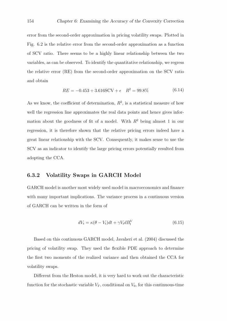
The generalized Dirac function and its derivative are important for our devel-
opments. Let δα(t) denote the generalized Dirac function, and δ(n)α (t) be its n-th
order derivative, then for a general smooth function ϕ(t):
∫ ∞
−∞δα(t)ϕ(t)dt = ϕ(α)∫ ∞
−∞δ(n)α (t)ϕ(t)dt = (−1)nϕ(n)(α)
(1.17)
We now introduce the Fourier transform and its generalization. The basic
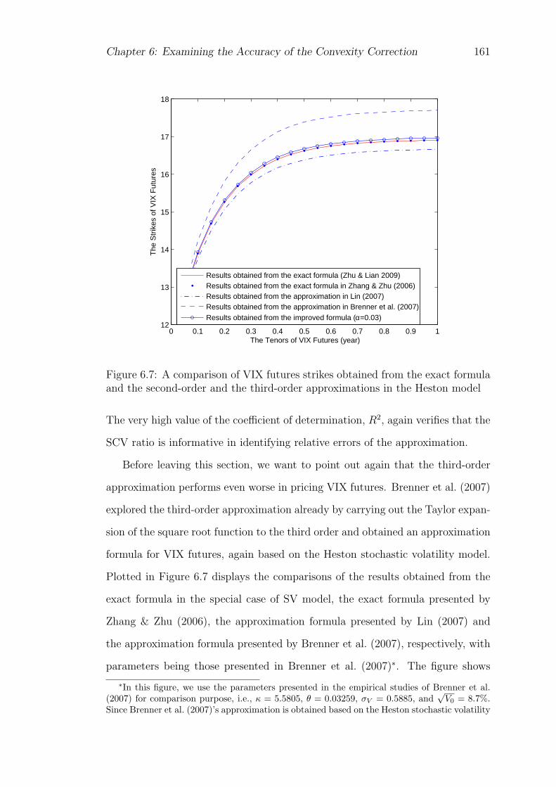
Chapter 1: Introduction and Background 15
definitions of Fourier transform and its inversion are given by
F [ϕ(t)]|ω =
∫ ∞
−∞ϕ(t)e−jωtdt,
F−1[ϕ(ω)]|t =1
2π
∫ ∞
−∞ϕ(ω)ejωtdω
(1.18)
Unfortunately, with this basic definition of Fourier transform, it is even not
possible to perform transform to some fundamental functions, such as the real
exponential function et, or the payoff function of a vanilla European option
max (S −K, 0). So we need to consider a generalization of Fourier transform
(see, e.g., Lewis 2000; Poularikas 2000 for more details). We first define a set of
rapidly decreasing test functions Φ that satisfies the following two properties:
1. Each test function in Φ is an analytical test function on the entire complex
plane;
2. Each test function, ϕ(x+ jy), in Φ satisfies
ϕ(x+ jy) = O(e−γ|x|) asx→ ±∞ (1.19)
for every real of y and γ.
It can be verified that every rapidly decreasing test function ϕ(t) in Φ is clas-
sical transformable. The generalized Fourier transform of a function f , F [f(t)]|ω,
is the function that satisfies the following equation
∫ ∞
−∞F [f(t)]|ωϕ(ω)dω =
∫ ∞
−∞f(y)F [ϕ(t)]|ydy (1.20)
for every rapidly decreasing test function ϕ(t) in Φ. Likewise, if G(ω) is a function
for which the following equation
∫ ∞
−∞F−1[G(ω)]|tϕ(t)dt =
∫ ∞
−∞G(y)F−1[ϕ(ω)]|ydy (1.21)
is well defined for every rapidly decreasing test function ϕ(t) in Φ, then F−1[G(ω)]|t
16 Chapter 1: Introduction and Background
is the generalized inverse Fourier transform of G(ω).
Using this generalized definition of Fourier transform, it can be shown that
for any complex value, α+ jβ,
F [ej(α+jβ)t]|ω = 2πδα+jβ(ω) (1.22)
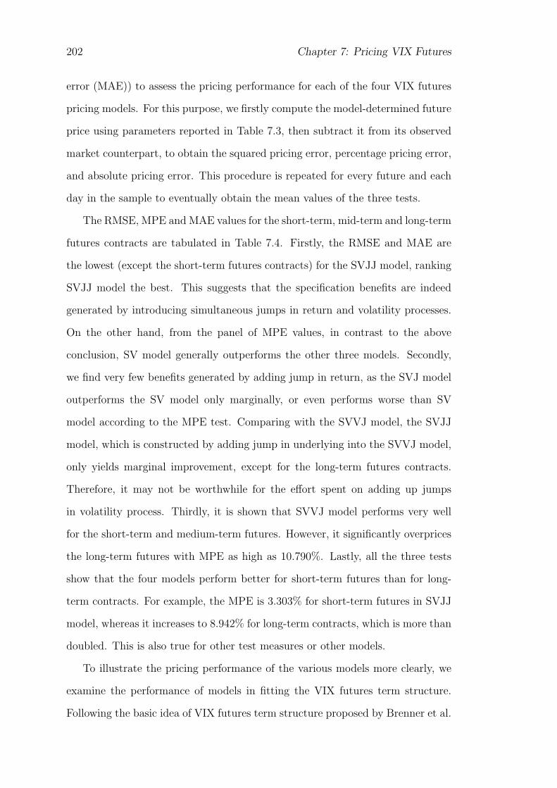
and
F [δj(t)]|ω = eω (1.23)
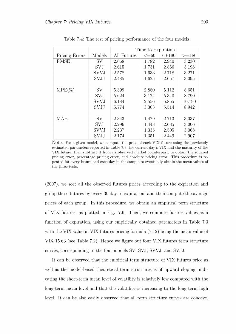
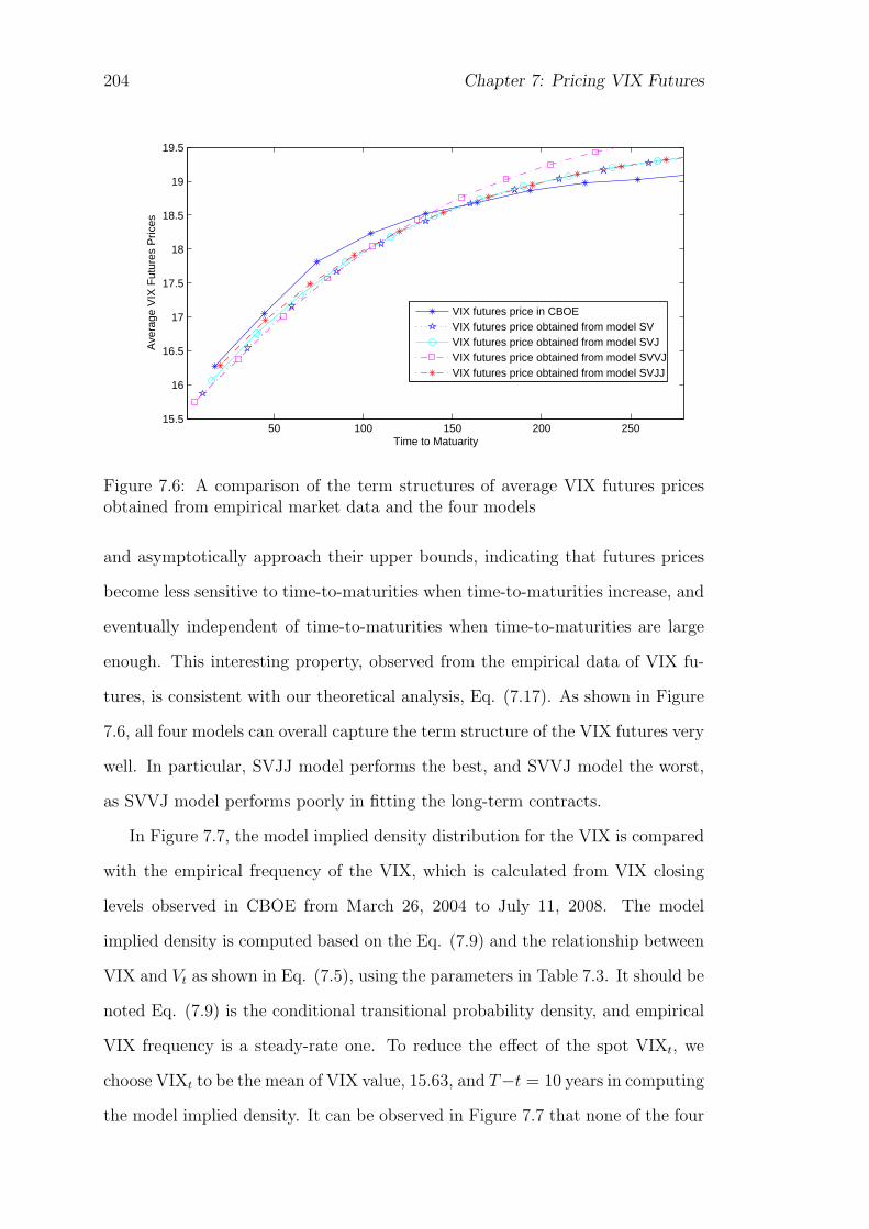
1.2.5 Characteristic Function
Now we start to introduce the characteristic function, which plays a vital role for
a real-valued random variable in probability theory.
The characteristic function of a real-valued random variable S is defined by
f(ϕ) = EQ[eiϕS] =
∫ ∞
−∞eiϕxp(x)dx (1.24)
Actually, the characteristic function is the Fourier transform of the probability
density function p(x) of the random variable S. The characteristic function of a
random variable completely characterizes the distribution of a random variable;
two variables with the same characteristic function are identical distributed. Fur-
thermore, a characteristic function is always continuous and satisfies f(0) = 1.
More importantly, the corresponding probability density function p(x) and cu-
mulative density function P (x) can be obtained by inverting the characteristic
function f(ϕ),
p(x) =1
2π
∫ ∞
−∞e−iϕxf(ϕ)dϕ (1.25)
and
P (x) = Prob(S ≤ x) =1
2− 1
π
∫ ∞
0
Re
[e−iϕxf(ϕ)
ϕi
]dϕ (1.26)
The reason that the characteristic function is important in mathematical fi-
Chapter 1: Introduction and Background 17
nance is the transitional probability density function is usually difficult to be
found analytically, whereas its Fourier transform (i.e., the characteristic func-
tion), is comparatively easy to be obtained. Since the terminal condition for the
characteristic function is the well smooth exponential function, its corresponding
PDE is comparatively easier to be solved. With the help of the characteristic
function, it is therefore convenient to switch the computation to the frequency
domain to solve the option pricing problems. For example, Heston (1993) de-
termined the price of an vanilla European call option by obtaining the explicit
solution of the characteristic function, based on a stochastic volatility model.
1.3 Mathematical Models
A good pricing model should produce the price of a financial derivative which
are very close to the real market price of the this contract. The prices of exotic
options given by models based on Black-Scholes assumptions can be wildly inac-
curate because they are frequently even more sensitive to levels of volatility than
standard European calls and puts. Therefore currently traders or dealers of these
financial instruments are motivated to find models to price options which take
the volatility smile and skew in to account. To this extent, stochastic volatility
models are partially successful because they can capture, and potentially explain,
the smiles, skews and other structures which have been observed in market prices
for options. In this section, we shall have an overview of these pricing models for
financial derivatives.
1.3.1 Black-Scholes Model
The Black-Scholes exponential Brownian motion model provides an approximate
description of the behaviour of asset prices and serves as a benchmark against
which other models can be compared. However, volatility does not behave in the
way the Black-Scholes equation assumes; it is not constant, it is not predictable, it
18 Chapter 1: Introduction and Background
is not even directly observable. Plenty of evidence exists that returns on equities,
currencies and commodities are not normally distributed, they have higher peaks
and fatter tails. Volatility has a key role to play in the determination of risk and
in the valuation of derivative securities. This section reviews the Black & Scholes
(1973) arbitrage argument from option valuation under constant volatility. This
allows us to introduce some frequently used notation and provides a basis for
the generalization to stochastic volatility. Black & Scholes (1973) model assumes
that the stock price satisfies the following stochastic differential equation(SDE):
dS = µSdt+ σSdW (1.27)
where µ is the deterministic instantaneous drift or return of the stock price, and
σ is the volatility for the stock price.
In the Black & Scholes (1973), it is also assumed that there is a money market
security (bank account) paying continuously compounded annual rate r and se-
curity markets are perfect so that one can trade continuously with no transaction
costs and no arbitrage opportunities∗∗.
Under these assumptions, one can construct a portfolio consisting of one Eu-
ropean option C with arbitrary payoff C(S, T ) = Ψ(S) and a number −ϕ of an
underlying asset. The value of the portfolio at time t is:
Π = C − ϕS (1.28)
where ϕ is a constant and makes Π instantaneously risk-free. The jump of the
value of this portfolio in one infinitesimal time step is:
dΠ = dC − ϕdS (1.29)
∗∗There are never any opportunities to make an instantaneous risk-free profit. “There is nosuch things as free lunch”.
Chapter 1: Introduction and Background 19
Hence by the principle of no arbitrage, Π must instantaneously earn the risk-free
bank rate r:
dΠ = rΠdt (1.30)
The central idea of the Black-Scholes argument is to eliminate the stochastic
component of risk by making the number of shares equal to:
ϕ =∂C
∂S(1.31)
Applying Ito’s lemma to C(S, t) and with some substitutions, one gets
∂C
∂t+
1
2S2σ2∂
2C
∂S2+ rS
∂C
∂S= rC (1.32)
This is the Black-Scholes equation and is a linear parabolic partial differential
equation. In fact, almost partial dierential equations in finance are of a similar
form. One of the attractions of the Black-Scholes equation is that the option price
function is independent of the expected return of the stock µ. The Black-Scholes
equation was first written down in 1969, but the derivation of the equation was
finally published in 1973.
The payoff for a European (vanilla) call option with strike K is C(S, T ) =
max (S −K, 0), and the option’s price at time t has an analytic or closed-form
solution (i.e., the Black-Scholes formula) by solving the Black-Scholes equation
in the form:
C(S, t) = SN(d1)−Ke−r(T−t)N(d2) (1.33)
where
d1 =log ( S
K) + (r + 1
2σ2)(T − t)
σ√T − t
d2 = d1 − σ√T − t
(1.34)
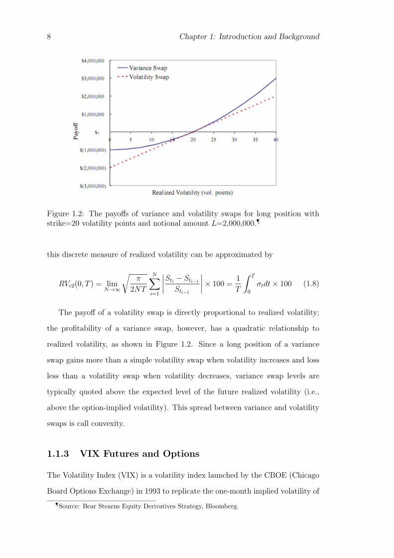
20 Chapter 1: Introduction and Background
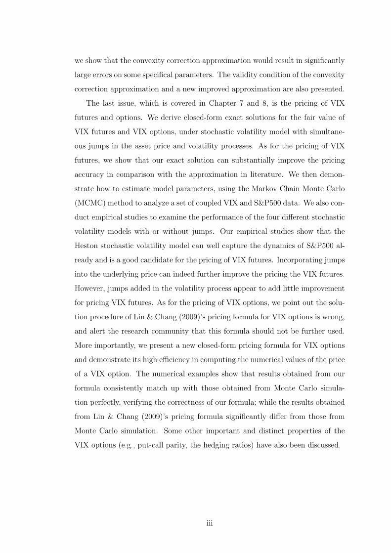
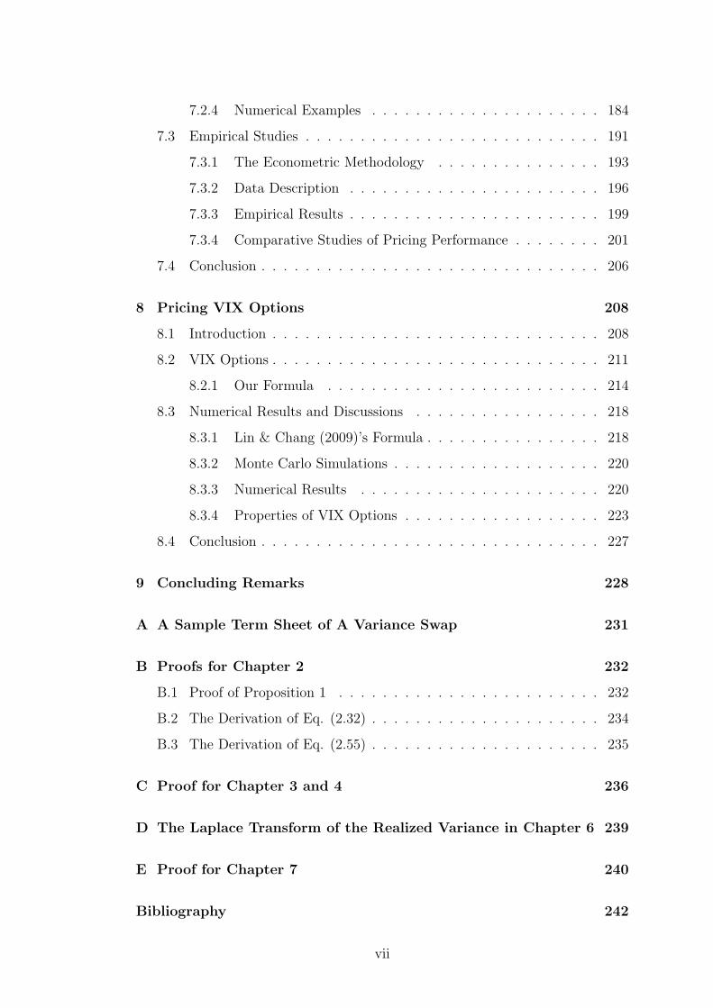
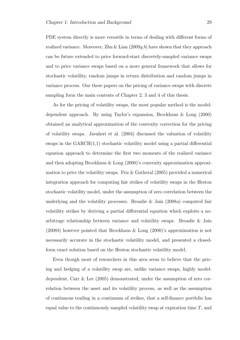
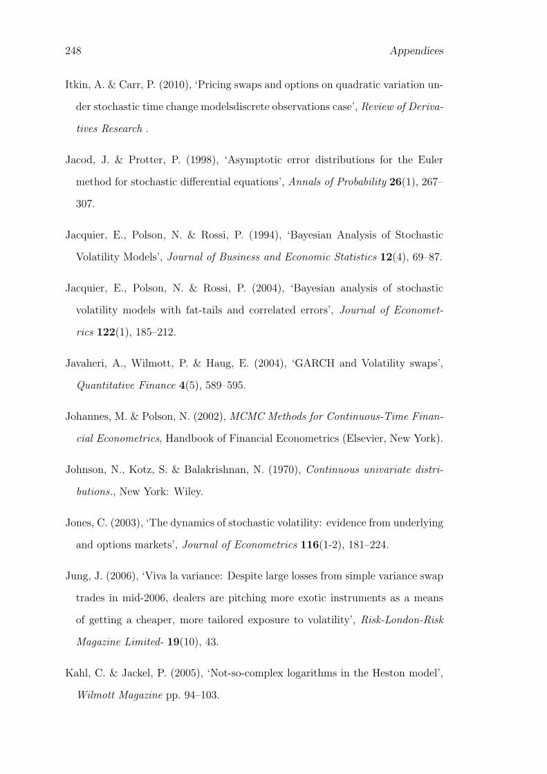
4300 4350 4400 4450 4500 4550 4600 46500.294
0.296
0.298
0.3
0.302
0.304
0.306
Strike Prices of Call Options
Impl
ied
Vol
atili
ty
Implied Volatility of Call Options (Expiration τ = 1 month)
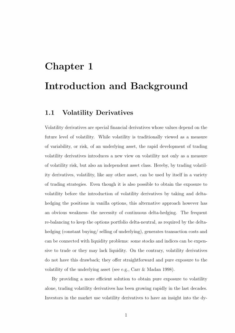
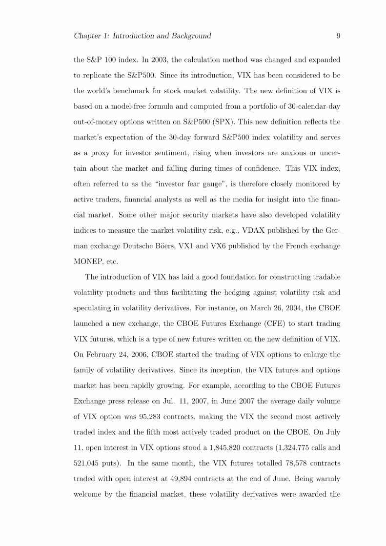
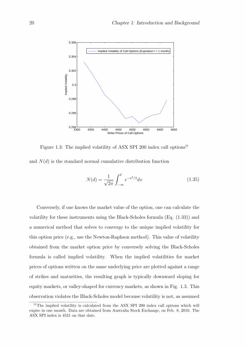
Figure 1.3: The implied volatility of ASX SPI 200 index call options††
and N(d) is the standard normal cumulative distribution function
N(d) =1√2π
∫ d
−∞e−x2/2dx (1.35)
Conversely, if one knows the market value of the option, one can calculate the
volatility for these instruments using the Black-Scholes formula (Eq. (1.33)) and
a numerical method that solves to converge to the unique implied volatility for
this option price (e.g., use the Newton-Raphson method). This value of volatility
obtained from the market option price by conversely solving the Black-Scholes
formula is called implied volatility. When the implied volatilities for market
prices of options written on the same underlying price are plotted against a range
of strikes and maturities, the resulting graph is typically downward sloping for
equity markets, or valley-shaped for currency markets, as shown in Fig. 1.3. This
observation violates the Black-Scholes model because volatility is not, as assumed
††The implied volatility is calculated from the ASX SPI 200 index call options which willexpire in one month. Data are obtained from Australia Stock Exchange, on Feb. 8, 2010. TheASX SPI index is 4521 on that date.
Chapter 1: Introduction and Background 21
in Black-Scholes model, a deterministic quantity. Either the term “volatility
smile” or “volatility skew” may be used to refer to the general phenomena of
volatilities varying by strikes.
1.3.2 Local Volatility Model
There have been many approaches to remedy the drawback of the constant volatil-
ity assumption within the Black-Scholes model. The local volatility model, a con-
cept originated by Derman & Kani (1994), and Dupire (1994), treats volatility
as a function of the current asset level St and of time t, instead of a constant as
assumed in Black-Scholes model. Given the prices of call or put options across
all strikes and maturities, one can deduce the local volatility function to match
the theoretical option prices with the market prices. Dupire (1994) showed that
if the spot price follows a risk-neutral random walk of the form:
dS
S= rdt+ σ(S, t)dW (1.36)
and if no-arbitrage market prices for European vanilla options are available for all
strikes K and expiries T , then σL(K,T ) can be extracted analytically from these
option prices. If C(S, t,K, T ) denotes the price of a European call with strike K
and expiry T , Dupire’s famous equation is obtained:
∂C
∂T= σ2
L(K,T )K2
2
∂2C
∂K2− rK
∂C
∂K(1.37)
Rearranging this equation, the direct expression to calculate the local volatility
(Dupire formula) is obtained:
σ2L(K,T ) =
√∂C∂T
+ rK ∂C∂K
K2
2∂2C∂K2
(1.38)
22 Chapter 1: Introduction and Background
Unlike the naive volatility produced by applying the Black-Scholes formula to
market prices, the local volatility is the volatility implied by the market prices
and the one factor Black-Scholes. One potential problem of using the Dupire
formula (1.38) is that, for some financial instruments, the option prices of different
strikes and maturities are not available or not enough to calculate the right local
volatility. Another problem is for strikes far in- or out-the-money, the numerator
and denominator of this equation may become very small, which could lead to
numerical inaccuracies.
1.3.3 Stochastic Volatility Models
Stochastic volatility models are conceptually quite different from the fitting ap-
proach of local volatility model. In these models, the volatility is neither a con-
stant as assumed in Black-Scholes model, nor a deterministic function of the
current asset level St and of time t as assumed in local volatility model. Rather,
it is by itself stochastic.
What is happening may be viewed in some different and related ways. Op-
tions prices are determined by supply and demand, not by theoretical formula.
The traders who are determining the option prices are implicitly modifying the
Black-Scholes assumptions to account for volatility that changes both with time
and with stock price level. This is contrary to the Black and Scholes (1973) as-
sumptions of constant volatility irrespective of stock price or time to maturity.
That is, traders assume σ = σ(St, t), whereas Black-Scholes model assumes that
σ is just a constant.
By imposing specific stochastic processes for both the stock price and its
instantaneous variance (or volatility), a stochastic volatility model is based on a
structural assumption on the underlying stock price. In this way, the stochastic
volatility model is to incorporate the empirical observation that volatility appears
not to be constant and indeed varies, at least in part, randomly, by making the
Chapter 1: Introduction and Background 23
volatility itself a stochastic process. The candidate models have generally been
motivated by intuition, convenience and a desire for tractability. In particular,
the popular Heston (1993) model assumes that the instantaneous variance of
the stock price is a square-root diffusion whose increments are correlated to the
increments of the return of the stock price. Other popular stochastic volatility
models are model by Stein & Stein (1991), model by Schobel & Zhu (1999),
GARCH diusion model (Lewis 2000), to name but a few. In addition, there are
also models which incorporate jump processes (see, for example, Merton 1976;
Madan et al. 1998) or mixtures of both concepts such as Bates (1996), Duffie
et al. (2000). Stochastic volatility on option values is similar to the effect of a
jump component: both increase the probability that out-of-the-money options
will finish in-the-money and vice versa (Wiggins 1987). Whether the smile is
skewed left, skewed right, or symmetrical in a stochastic volatility model depends
upon the sign of the correlation between changes in volatility and changes in stock
price (Hull & White 1987).
The stochastic nature of the instantaneous variance of the stock price process
is particular important if we want to price and hedge heavily volatility-dependent
exotic options such as options on realized variance or cliquet-type products. Such
products cannot be priced correctly in the BS-model since their very risklies in
the movement of volatility (or variance, for that matter) itself.
While Black and Scholes (BS) used only the underlying stock price and the
bond to hedge a derivative in their model, this cannot be justified anymore:
their model is not able to capture what is today known as the volatility skew or
volatility smile, of the implied volatility of traded vanilla options. The root of
the discrepancy is that volatility is not, as assumed in BS model, a deterministic
quantity. Rather, it is by itself stochastic.
dSt = µStdt+√VtStdB
St
dVt = κ(θ − Vt)dt+ σV√VtdB
Vt
(1.39)
24 Chapter 1: Introduction and Background
where µ is the deterministic instantaneous drift or return of the stock price,
and the variance V is correlated with the stock price by ρ, We cannot hold or
“short” volatility, but can hold a position in a second option to do hedging. So let
us consider the valuation of the volatility dependent instrument (e.g., volatility
swaps), assuming that one can take long or short positions in a second instrument
as well as in the underlying.
In the Black-Scholes case, there is only one source of randomness-the stock
price, which can be hedged with stock. In the present case, random changes in
volatility also need to be hedged in order to form a riskless portfolio. So we
setup a portfolio Π containing the option to be priced whose value is denote by
C(S, V, t), a quantity −ϕ1 of the stock and a quantity −ϕ2 of another asset whose
value U depends on volatility. We have
Π = C − ϕ1S − ϕ2U (1.40)
The change in this portfolio in a time increment dt is given by
dΠ = dC − ϕ1dS − ϕ2dU (1.41)
As by standard, one applies Ito’s Lemma to this portfolio to obtain
dΠ = adS + bdV + cdt (1.42)
where
a =∂C
∂S− ϕ1 − ϕ2
∂U
∂S, b =
∂C
∂S− ϕ1 − ϕ2
∂U
∂S
c = (∂C
∂t+
1
2S2V
∂2C
∂S2+ ρSσV V
∂2C
∂S∂V+
1
2σ2V V
∂2C
∂V 2)
−ϕ2(∂U
∂t+
1
2S2V
∂2U
∂S2+ ρSσV V
∂2U
∂S∂V+
1
2σ2V V
∂2U
∂V 2)
(1.43)
Clearly we wish to eliminate the stochastic component of risk by setting a =
Chapter 1: Introduction and Background 25
b = 0, so one can rearrange the hedge parameters in the form:
dΠ = adS + bdV + cdt (1.44)
where
ϕ1 =∂C
∂S− ϕ2
∂U
∂S
ϕ2 = (∂C
∂V)/(
∂U
∂V)
(1.45)
to eliminate the dS term and the dV term. The avoidance of the arbitrage, once
these choices of ϕ1 and ϕ2, are made, is the condition:
dΠ = rΠdt
dΠ = r(V − ϕ1S − ϕ2U)dt(1.46)
where we have used the fact that the return on a risk-free portfolio must be
equal to the risk-free bank rate which we will assume to be deterministic for our
purposes. Combining equations (2.14) and (2.15), collecting all C terms on the
left hand side and all U terms on the right hand side, one gets:
(∂C
∂t+
1
2V S2∂
2C
∂S2+ ρSσV V
∂2C
∂S∂V+
1
2σ2V V
∂2C
∂V 2+ rS
∂C
∂S− rC)/
∂C
∂V=
(∂U
∂t+
1
2V S2∂
2U
∂S2+ ρSσV V
∂2U
∂S∂V+
1
2σ2V V
∂2U
∂V 2+ rS
∂U
∂S− rU)/
∂U
∂V
(1.47)
The left-hand side is a function of C only and the right-hand side is a function
of U only. The only way that this can be is for both sides to be equal to some
function depending only on variables S, V and t. So, if one writes both sides as
f(S, V, t), in doing so, one arrives at the general PDE for stochastic volatility:
(∂C
∂t+
1
2V S2∂
2C
∂S2+ ρσV SV
∂2C
∂S∂V+
1
2σ2V V
∂2C
∂V 2+ rS
∂C
∂S− rC) = −(α− λβ)
∂C
∂V(1.48)
where, without loss of generality, we have written the arbitrary function f of S,
V and t as (α−λβ). Conventionally, λ is called the market price of volatility risk
because it tells us how much of the expected return of C is explained by the risk
26 Chapter 1: Introduction and Background
(i.e., standard deviation) of V in the Capital Asset Pricing Model framework.
1.4 Literature Review
1.4.1 Variance Swaps and Volatility Swaps
Since the sharp increase in the trading volume of variance swaps recently, it has
drawn considerable research interests to develop appropriate valuation approaches
for variance swaps. In the literature, there have been two types of valuation
approaches, numerical methods and analytical methods.
Of all the analytical methods, there are two subcategories. The most influ-
ential ones were proposed by Carr & Madan (1998) and Demeterfi et al. (1999).
They have shown how to theoretically replicate a variance swap by a portfolio
of standard options. Without requiring to specify the function of volatility pro-
cess, their models and analytical formulae are indeed very attractive. However, as
pointed out by Carr & Corso (2001), the replication strategy has a drawback that
the sampling time of a variance swap is assumed to be continuous rather than
discrete; such an assumption implies that the results obtained from a continuous
model can only be viewed as an approximation for the actual cases in financial
practice, in which all contacts are written with the realized variance being evalu-
ated on a set of discrete sampling points. Another drawback is that this strategy
also requires options with a continuum of exercise prices, which is not actually
available in marketplace. The second kind of analytical methods is the stochas-
tic volatility models. Grunbichler & Longstaff (1996) first developed a pricing
model for volatility futures based on mean-reverting squared-root volatility pro-
cess. Heston (2000) derived an analytical solution for both variance and volatility
swaps based on the GARCH volatility process. Javaheri et al. (2004) also dis-
cussed the valuation and calibration for variance swaps based on the GARCH(1,1)
stochastic volatility model. They used the flexible PDE approach to determine
Chapter 1: Introduction and Background 27
the first two moments of the realized variance in the context of continuous as
well as discrete sampling, and then obtained a closed-form approximate solution
after the so-called convexity correction was made. Howison et al. (2004) also
considered the valuation of variance swaps and volatility swaps under a variety
of diffusion and jump-diffusion models. In their work, approximate solutions of
the PDE for pricing volatility-related products are derived. Swishchuk (2004)
used an alternative probabilistic approach to value variance and volatility swaps
under the Heston (1993) stochastic volatility model. More recently Elliott et al.
(2007) proposed a model to evaluate variance swaps and volatility swaps un-
der a continuous-time Markov-modulated version of the stochastic volatility with
regime switching, with both probabilistic and PDE approaches being discussed.
All these stochastic volatility models, however, are based on the assumption that
the realized variance is approximated with a continuously-sampled one, which
will result in a systematic bias for the price of a variance swap. As will be shown
later, while the approximation methods provide fairly reasonable estimates for
the value of variance swaps with high sampling frequencies, they may lead to
large relative errors for variance swaps with small sampling frequencies or long
tenors.
Various numerical methods, as an alternative to analytical methods, were also
intensively developed recently. A typical article in this category belongs to Little
& Pant (2001). In their article, it is shown how to price a variance swap using
the finite-difference method in an extended Black-Scholes framework, in which
the local volatility is assumed to be a known function of time and spot price
of the underlying asset. By exploring a dimension reduction technique, their
numerical approach achieves high efficiency and accuracy for discretely-sampled
variance swaps. Windcliff et al. (2006) also explored a numerical algorithm to
evaluate discretely-sampled volatility derivatives using numerical partial-integro
differential equation approach. Under this framework, they investigated a variety
of modeling assumptions including local volatility models, jump-diffusion models
28 Chapter 1: Introduction and Background
and models with transaction cost being taken into consideration. Although these
two numerical methods evaluate variance swaps based on discretely-sampled real-
ized variance and achieve high accuracy, the major limitation is that their models
do not incorporate stochastic volatilities that are the most commonly used to
model the dynamics of equity indices. To remedy this drawback, Little & Pant
(2001) and Windcliff et al. (2006) pointed out, respectively, in the conclusions
of their papers that for better pricing and hedging general variance swaps one
needs to adopt an appropriate model that incorporates the stochastic volatility
characteristics observed in financial markets.
To properly address this discretely sampling effect, several works have been
done very recently. Broadie & Jain (2008b) presented a closed-form solution for
volatility as well as variance swaps with discrete sampling. They also examined
the effects of jumps and stochastic volatility on the price of volatility and variance
swaps by comparing calculated prices under various models such as the Black-
Scholes model, the Heston stochastic volatility model, the Merton (1973) jump
diffusion model and the Bates (1996) and Scott (1997) stochastic volatility and
jump model. However, their solution approach is primarily based on integrating
the underlying stochastic processes directly and it appears that it can only be
used when the realized variance is defined in such a particular form that the
stochastic processes assumed for the underlying can happen to be exactly the
same as that defined in the calculation of the realized variance. In other words,
Broadie & Jain (2008b)’s approach can only be used when the realized variance
is defined as the average of the squared log returns (Eq. (1.1)), as Zhu & Lian
(2009d) pointed out.
On the other hand, Zhu & Lian (2009d,f) presented an completely different
approach to obtain two closed-form formulae for variance swaps based on the
two different definitions of discretely-sampled realized variance (Eq. (1.1 and
(1.2)), under the Heston (1993)’s stochastic volatility model. Unlike Broadie &
Jain (2008b)’s approach, Zhu & Lian (2009d)’s approach of solving the governing
Chapter 1: Introduction and Background 29
PDE system directly is more versatile in terms of dealing with different forms of
realized variance. Moreover, Zhu & Lian (2009g,b) have shown that they approach
can be future extended to price forward-start discretely-sampled variance swaps
and to price variance swaps based on a more general framework that allows for
stochastic volatility, random jumps in return distribution and random jumps in
variance process. Our these papers on the pricing of variance swaps with discrete
sampling form the main contents of Chapter 2, 3 and 4 of this thesis.
As for the pricing of volatility swaps, the most popular method is the model-
dependent approach. By using Taylor’s expansion, Brockhaus & Long (2000)
obtained an analytical approximation of the convexity correction for the pricing
of volatility swaps. Javaheri et al. (2004) discussed the valuation of volatility
swaps in the GARCH(1,1) stochastic volatility model using a partial differential
equation approach to determine the first two moments of the realized variance
and then adopting Brockhaus & Long (2000)’s convexity approximation approxi-
mation to price the volatility swaps. Friz & Gatheral (2005) provided a numerical
integration approach for computing fair strikes of volatility swaps in the Heston
stochastic volatility model, under the assumption of zero correlation between the
underlying and the volatility processes. Broadie & Jain (2008a) computed fair
volatility strikes by deriving a partial differential equation which exploits a no-
arbitrage relationship between variance and volatility swaps. Broadie & Jain
(2008b) however pointed that Brockhaus & Long (2000)’s approximation is not
necessarily accurate in the stochastic volatility model, and presented a closed-
form exact solution based on the Heston stochastic volatility model.
Even though most of researchers in this area seem to believe that the pric-
ing and hedging of a volatility swap are, unlike variance swaps, highly model-
dependent, Carr & Lee (2005) demonstrated, under the assumption of zero cor-
relation between the asset and its volatility process, as well as the assumption
of continuous trading in a continuum of strikes, that a self-finance portfolio has
equal value to the continuously sampled volatility swap at expiration time T , and
30 Chapter 1: Introduction and Background
hence developed model-free trading strategies to price and replicate volatility
swaps.
Papers focusing on analytically pricing discretely-sampled volatility swaps are
rare in literature, mainly due to the inherent difficulty associated with the non-
linearity in the pay-off function. Zhu & Lian (2009c) present a closed-form exact
solution for the pricing of discretely-sampled volatility swaps, under the frame-
work of Heston (1993) stochastic volatility model, based on the definition of the
so-called average of realized volatility (Eq. (1.7)). As for the standard deriva-
tion volatility swaps, in which the realized volatility is defined as the square root
of the realized variance as shown in Eq. (1.5), there is no exact solution avail-
able at all for the discretely-sampled volatility swaps. Broadie & Jain (2008b)
presented a closed-form approximation to price continuously-sampled standard
derivation volatility swaps (Eq. (1.6)), based on the Heston model. A more com-
mon approach in literature is Brockhaus & Long (2000)’s convexity correction
approximation. Zhu & Lian (2010e) systematically investigated the accuracy and
the validity condition of the convexity correction approximation, through both
theoretical analysis and numerical examples, and found out this approximation
on some specifical parameters would result in significantly large errors. They also
presented a new approximation, which is an extension of the convexity correction
formula, to improve the accuracy. The Chapter 5 and 6 of this thesis are based
on these two recent papers of ours (i.e., Zhu & Lian 2009c, 2010e).
1.4.2 VIX Futures and Options
Given the growing popularity of trading VIX futures, considerable research in-
terests have also been drawn to the development of appropriate pricing models
for VIX futures. Grunbichler & Longstaff (1996) first developed a pricing model
for volatility futures and volatility options based on a mean-reverting squared-
root volatility process. Carr & Wu (2006) presented a lower bound and an upper
Chapter 1: Introduction and Background 31
bound for the price of VIX futures. By using the Jensen’s inequality, they have
shown that the lower bound is the forward-starting volatility swap rate (strike
price) and the upper bound is the squared root of forward-starting variance swap
rate over the period (t, t+ 30/365). Dupire (2005) derived the convexity adjust-
ment that needs to be subtracted from the price of forward variance to arrive at
the fair value of VIX futures. Zhang & Zhu (2006) proposed an expression for
VIX futures, assuming S&P500 is modeled by Heston (1993)’s stochastic volatil-
ity. Zhu & Zhang (2007) further derived a no-arbitrage pricing model for VIX
futures based on the variance term structure. Lin (2007) presented a convexity
adjustment approximation for the value of the VIX futures under various stochas-
tic volatility models with simultaneous jumps both in the asset price and variance
processes. Psychoyios et al. (2007) provided a pricing model for both VIX futures
and VIX options based on the squared root mean reverting process with jumps.
Brenner et al. (2007) used market data to establish the relationship between the
VIX futures prices and the VIX itself. They further theoretically explained the
relationship between VIX and VIX futures, the valuation of VIX futures and
model calibration, based on Heston (1993)’s stochastic volatility model. Sepp
(2008a, 2008b) applied the square root stochastic variance model with variance
jumps to describe the evolution of S&P500 volatility, and demonstrated how to
apply the model to the pricing and hedging of VIX futures and options. Some
other typical recent papers about the VIX and its derivatives (futures and op-
tions) include Zhang et al. (2010), Zhang & Huang (2010), Lu & Zhu (2009),
Carr & Lee (2009) etc.
Zhu & Lian (2009a) recently derived a closed-form exact solution for the fair
value of VIX futures under stochastic volatility model with simultaneous jumps
in the asset price and volatility processes. With the newly-found pricing formula
available, especially with its great computational efficiency, we are also able to
conduct empirical studies, aiming at examining the performance of four different
stochastic volatility models with or without jumps. More importantly, using the
32 Chapter 1: Introduction and Background
Markov Chain Monte Carlo (MCMC) method to analyze a set of coupled VIX
and S&P500 data, we demonstrate how to estimate model parameters. Through
these empirical studies, we are able to compare the pricing performance of four
models, of which analytical pricing formulae have been found and presented in
this chapter. The Chapter 7 of this thesis is based on our this paper (i.e., Zhu &
Lian 2009a).
Lin & Chang (2009) presented a closed-form pricing formula for VIX options
that reconcile the most general price processes of the S&P500 in the literature:
stochastic volatility, price jumps, and volatility jumps. Utilizing this closed-form
pricing formula for VIX options, they empirically investigated how much each
generalization of the S&P500 price dynamics improves VIX option pricing, and
concluded that a model with stochastic volatility and state-dependent correlated
jumps in S&P500 returns and volatility (i.e., Duffie et al. 2000) is a better alter-
native to the others in terms of pricing VIX options. By applying the exactly
same pricing formula for VIX options shown in Lin & Chang (2009), Lin & Chang
(2010) further studied the relationships among stylized features on S&P 500, VIX
and options on VIX, and examined how jump factors impact VIX option pricing
and hedging. Zhu & Lian (2010b), however, pointed out that the correctness
of the formula proposed in Lin & Chang (2009) is in serious doubt. Using a
completely different approach from Lin & Chang (2009), they presented an an-
alytical exact solution for the price of VIX options under stochastic volatility
model with simultaneous jumps in the asset price and volatility processes. They
also offered numerical results to illustrate the correctness of their formula, and
the incorrectness of the formula in Lin & Chang (2009).
1.5 Structure of Thesis
In this thesis, we develop some highly efficient approaches to analytically price
volatility derivatives. In particular, using our approach, we present a set of closed-
Chapter 1: Introduction and Background 33
form exact pricing formulae for discretely-sampled variance swaps, forward-start
variance swaps, volatility swaps and VIX futures and options.
In Chapter 2, we present two closed-form exact solutions to price variance
swaps with discrete sampling times by solving the partial differential equation
(PDE) system based on the Heston (1993) two-factor stochastic volatility model,
embedded in the framework proposed by Little & Pant (2001). In comparison
with all the previous approximation models based on the assumption of con-
tinuous sampling time, the current research of working out closed-form exact
solutions for variance swaps with discrete sampling times at least serves for two
major purposes: (i) to verify the degree of validity of using a continuous-sampling-
time approximation for variance swaps of relatively short sampling period; (ii) to
demonstrate that significant errors can result from still adopting such an assump-
tion for a variance swap with small sampling frequencies or long tenor. Other
key features of our new solution approach include: (a) with the newly found an-
alytic solutions, all the hedging ratios of a variance swap can also be analytically
derived; (b) numerical values can be very efficiently computed from the newly
found analytic formula.
In Chapter 3, a more general and condense approach is presented to price
forward-start variance swaps with discrete sampling times, based on the Heston
(1993) two-factor stochastic volatility model. By developing the forward charac-
teristic function, it is shown this approach possesses some great advantages over
those in literature: (1) treating the pricing problem of variance swaps with dif-
ferent definitions of discretely-sampled realized variance in a highly unified way;
(2) easily obtaining analytical closed-form solutions for forward-start variance
swaps with two popularly-used definitions of discretely-sampled realized variance;
(3) enabling the investigation of some important properties of the forward-start
variance swaps, utilizing the elegant and simple form of the obtained solutions.
Thereby, this work represents a substantial progress in the field of pricing variance
swaps.
34 Chapter 1: Introduction and Background
In Chapter 4, we extend the approach in Chapter 3 to price discretely-sampled
variance by further including random jumps in the return and volatility processes,
and present two new closed-form exact solutions for the prices of variance swaps
with discrete sampling times based on the Heston stochastic volatility and random
jumps in the return and volatility processes. By working out the closed-form ex-
act solutions for such a general model with jumps being possibly included in both
the underlying and the variance, our new formulae for the two most commonly-
adopted definitions of discretely-sampled realized variance can serve to improve
the computational speed and accuracy in pricing variance swaps as well as in
model calibration using stochastic volatility models with jumps. The fact that
the newly-derived formulae can cover a wide range of models proposed in the
literature, i.e., either with jumps being included in the underlying process or in
the variance process or both, further demonstrate that our approach is a highly
versatile and unified approach that can be used for pricing discretely-sampled
variance swaps. Utilizing our new closed-form exact solutions, we have also con-
ducted some cross-model comparison, examining various parameters involved in
the jump processes.
In Chapter 5, we present a closed-form exact solution for the pricing of
discretely-sampled volatility swaps, under the framework of Heston (1993) stochas-
tic volatility model, based on the definition of the so-called average of realized
volatility. Papers focusing on analytically pricing discretely-sampled volatility
swaps are rare in literature, mainly due to the inherent difficulty associated with
the nonlinearity in the pay-off function. By working out such a closed-form exact
solution for discretely-sampled volatility swaps, this work has: (1) significantly
reduced the computational time in obtaining numerical values for the discretely-
sampled volatility swaps; (2) substantially improved the computational accuracy
of discretely-sampled volatility swaps, comparing with the continuous sampling
approximation; (3) enabled all the hedging ratios of a volatility swap to be also
analytically derived.
Chapter 1: Introduction and Background 35
In Chapter 6, we investigate another important issue in pricing volatility
swaps. Convexity correction is a well-known approximation technique used in
pricing volatility swaps. However, studies focusing on examining the accuracy
of the technique itself are rare and the validity condition of this convexity cor-
rection approximation was hardly addressed and discussed in literature. In this
chapter, we systematically investigate the accuracy and the validity condition of
the convexity correction approximation, through both theoretical analysis and
numerical examples. Hereby, our study answers the two basic questions in adopt-
ing the convexity correction approximation to derive approximate formula for
pricing variance or volatility swaps: (a) why and when the convexity correction
approximation will result in significantly large errors. In other words, what is
the validity condition of applying the convexity correction approximation; (b)
a better accuracy cannot be achieved by extending the convexity correction ap-
proximation, which is the second-order Taylor expansion, to third order or fourth
order Taylor expansions. Some other contributions of this study include: (1)
alerting that one should be aware of the inaccuracy of this approximation and be
very careful in using it; (2) a new approximation, which is an extension of the
convexity correction approximation, has been proposed to improve the accuracy.
In Chapter 7, we price VIX futures by deriving a closed-form exact solution for
the fair value of VIX futures under stochastic volatility model with simultaneous
jumps in the asset price and volatility processes. Since the inception of the
volatility index (VIX) by the CBOE in 1993, in particular, the introduction of the
VIX futures by CBOE in 2004, various pricing models with stochastic volatilities
have been proposed to value VIX futures. However, rarely could an analytic
closed-form solution be found, especially for models that include jumps in both
VIX and its volatility. Thus the derivation of this formula for VIX futures with a
very general dynamics of VIX represents a substantial progress in identifying and
developing more realistic VIX futures models and pricing formulae. With the
newly-found pricing formula available, especially with its great computational
36 Chapter 1: Introduction and Background
efficiency, we are also able to conduct empirical studies, aiming at examining the
performance of four different stochastic volatility models with or without jumps.
More importantly, using the Markov Chain Monte Carlo (MCMC) method to
analyze a set of coupled VIX and S&P500 data, we demonstrate how to estimate
model parameters, which is a crucial step for any fancy mathematical model to
be of practical use. Through these empirical studies, we are able to compare the
pricing performance of four models, of which analytical pricing formulae have
been found and presented in this chapter.
In the Chapter 8, we demonstrate the derivation of an analytical exact solution
for the price of VIX options under stochastic volatility model with simultaneous
jumps in the asset price and volatility processes. We point out that the solution
procedure of Lin & Chang (2009)’s pricing formula for VIX options is incorrect.
Our approach presented in this chapter is totally different from the approach in
Lin & Chang (2009) in obtaining a closed-form pricing formula for VIX options.
We then show that the numerical results obtained from our formula consistently
match up with those obtained from Monte Carlo simulation perfectly, verifying
the correctness of our formula. However the results obtained from Lin & Chang
(2009)’s pricing formula significantly differ from those from Monte Carlo simu-
lation, confirming our doubt that their pricing formula is incorrect. It is shown
that our pricing formula is very efficient in computing the numerical prices of VIX
options. Some important and distinct properties of the VIX options (e.g., put-call
parity, the hedging ratios) have also been discussed in this chapter. Therefore,
our formula can be a very useful tool in trading practice when there is obviously
increasing demand of trading VIX options in financial markets.
Chapter 2
Pricing Variance Swaps with
Discrete Sampling
2.1 Introduction
The trading volume of variance swaps has been experiencing a sharp increase
recently. This has drawn considerable research interests to develop appropriate
valuation approaches for variance swaps. However, most of the studies in liter-
ature are based on the assumption that the realized variance is approximated
with a continuously-sampled one, as discussed in Chapter 1. In this chapter, we
price discretely-sampled variance swaps based on Heston’s two-factor stochastic
volatility model embedded in Little & Pant’s (2001) framework. Unlike Broadie
& Jain (2008b)’s approach, our approach presented here is much simpler by solv-
ing the governing PDE system directly and is more versatile in terms of dealing
with different forms of realized variance. In this way, the nature of stochastic
volatility is included in the model and most importantly, two closed-form exact
solutions can be worked out, even when the sampling times are discrete, for the
corresponding two definitions of the discretely-sampled realized variance.
Furthermore, it is shown that our solutions degenerate to continuous sampling
model when sampling frequency approaches infinity, as expected. Our explicit
37
38 Chapter 2: Pricing Variance Swaps with Discrete Sampling
pricing formulae for variance swaps presented here should be valuable in both
theoretical and practical senses. Theoretically, although there are many existing
models, as mentioned above, to price variance swaps, the closed-form exact so-
lutions for discretely-sampled variance swaps are presented for the first time in
the stochastic volatility framework. Secondly, our discrete model can be used to
verify the validity of the corresponding continuous models for the specific pay-off
discussed here and thus would fill a gap that has been in the field of pricing
variance swaps. Thirdly, the Fourier inverse transform in our model has been
analytically worked out, which is a significant step forward in the literature of
Heston’s model. Practically, the final form of our solution is simple enough in a
closed form and thus can be easily used by market practitioners. Furthermore,
our explicit solution shows substantial advantage, in terms of both accuracy and
efficiency, over previous numerical or approximate approaches, and thus it can
satisfy the increasing demand of trading variance swaps in financial markets.
This chapter is organized into four sections. In Section 2.2, a detailed descrip-
tion of variance swaps is first provided, followed by our analytical formulae for
the variance swaps. In Section 2.3, some numerical examples are given, demon-
strating the correctness of our solutions from various aspects. Comparison with
continuous sampling models and discussion for other properties of the variance
swaps are also carried out. In Section 2.4, a brief summary is provided.
2.2 Pricing Variance Swaps
In this section, we use the Heston (1993) stochastic volatility model to describe
the dynamics of the underlying asset. To evaluate the discretely-sampled realized
variance swaps, we employ the dimension reduction technique proposed by Little
& Pant (2001) to analytically solve the associated PDE and hence obtain closed-
form analytical solutions for fair strike prices of variance swaps with discrete
sampling.
Chapter 2: Pricing Variance Swaps with Discrete Sampling 39
2.2.1 The Heston Stochastic Volatility Model
It is a well-known fact by now that the Black & Scholes (1973) model may fail to
reflect certain features of the reality of financial markets due to some unrealistic
assumptions, such as the constant volatility assumption; numerous phenomena
such as smile effect (Wilmott 1998), skewness and kurtosis effects (Voit 2005) have
been observed and reported, suggesting necessary improvements of the Black-
Scholes model.
In the hope of remedying some apparent drawback of the Black-Scholes model,
many models have been proposed to incorporate stochastic volatility, stochastic
volatility with jump, stochastic volatility and stochastic interest rate (c.f., Stein
& Stein 1991; Heston 1993; Scott 1997; Schobel & Zhu 1999). In order to assess
the performance of these models, Bakshi et al. (1997) systematically analyzed the
performance of incorporating stochastic volatility, jump diffusion, and stochastic
interest rate, and concluded that the most important improvement over the Black-
Scholes model was achieved by introducing stochastic volatility into option pricing
models. Once this is done, introducing jumps and stochastic interest rate leads to
only marginal improvement in option pricing. For this reason, we shall focus on
the stochastic volatility model in this chapter, leaving stochastic volatility with
jump diffusions model to be discussed in Chapter 4. Among all the stochastic
volatility models in the literature, model proposed by Heston (1993) has received
the most attention since it can give a satisfactory description of the underlying
asset dynamics (Daniel et al. 2005; Silva et al. 2004). In the Heston (1993)
model, the underlying asset St is modeled by the following diffusion process with
a stochastic instantaneous variance Vt. dSt = µStdt+√VtStdB
St
dVt = κ(θ − Vt)dt+ σV√VtdB
Vt
(2.1)
where µ is the expected return of the underlying asset, θ is the long-term mean
40 Chapter 2: Pricing Variance Swaps with Discrete Sampling
of variance, κ is a mean-reverting speed parameter of the variance, σV is the
so-called volatility of volatility. The two Wiener processes dBSt and dBV
t describe
the random noise in asset and variance respectively. They are assumed to be
correlated with a constant correlation coefficient ρ, that is (dBSt , dB
Vt ) = ρdt.
The stochastic volatility process is the familiar squared-root process. To ensure
the variance is always positive, it is required that 2κθ ≥ σ2 (see Cox et al. 1985;
Heston 1993; Zhang & Zhu 2006).
According to the existence theorem of equivalent martingale measure, we are
able to change the real probability measure to a risk-neutral probability measure
and describe the processes as:
dSt = rStdt+√VtStdB
St
dVt = κQ(θQ − Vt)dt+ σV√VtdB
Vt
(2.2)
where κQ = κ+λ and θQ = κθκ+λ
are the risk-neutral parameters, the new param-
eter λ is the premium of volatility risk (Heston 1993). As illustrated in Heston’s
paper, applying Breeden (1979)’s consumption-based model yields a volatility
risk premium of the form λ(t, St, vt) = λV for the CIR square-root process. For
the rest of this chapter, our analysis will be based on the risk-neutral probability
measure. The conditional expectation at time t is denoted by EQt = EQ[· | Ft],
where Ft is the filtration up to time t.
2.2.2 Variance Swaps
As discussed in Chapter 1, variance swaps are forward contracts on the future
realized variance of the returns of the specified underlying asset. The value of a
variance swap at expiry can be written as (RV −Kvar)×L, where the RV is the
annualized realized variance over the contract life [0, T ], Kvar is the annualized
delivery price for the variance swap, which is set to make the value of a variance
swap equal to zero for both long and short positions at the time the contract
Chapter 2: Pricing Variance Swaps with Discrete Sampling 41
is initially entered. To a certain extent, it reflects market’s expectation of the
realized variance in the future. L is the notional amount of the swap in dollars
per annualized volatility point squared and T is the life time of the contract. For
more details about the variance swaps and variance futures, readers are referred
to the web sites of CBOE∗ or NYSE Euronext†.
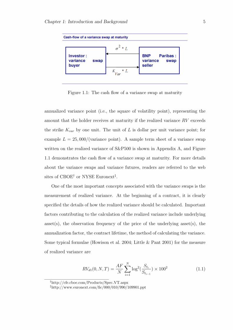
At the beginning of a contract, it is clearly specified the details of how the
realized variance should be calculated. Important factors contributing to the
calculation of the realized variance include underlying asset(s), the observation
frequency of the price of the underlying asset(s), the annualization factor, the
contract lifetime, the method of calculating the variance. Some typical formulae
(Howison et al. 2004; Little & Pant 2001) for the measure of realized variance are
RVd1(0, N, T ) =AF
N
N∑i=1
(Sti − Sti−1
Sti−1
)2
× 1002 (2.3)
or
RVd2(0, N, T ) =AF
N
N∑i=1
log2(Sti
Sti−1
)× 1002 (2.4)
where Sti is the closing price of the underlying asset at the i -th observation
time ti, and there are altogether N observations. AF is the annualized factor
converting this expression to an annualized variance. If the sampling frequency
is every trading day, then AF = 252, assuming there are 252 trading days in one
year, if every week then AF = 52, if every month then AF = 12 and so on. We
assume equally-spaced discrete observations in this thesis so that the annualized
factor is of a simple expression AF = 1∆t
= NT.
In the literature, these two definitions have been alternatingly used to mea-
sure the realized variance, even though in practice most of the contracts appear
to be drawn up using the definition RVd2(0, N, T ) for the realized variance. For
example, while Little & Pant (2001) used RVd1(0, N, T ) in their numerical method
T = 1 in this section. This set of parameters for the square root process was
also adopted by Dragulescu & Yakovenko (2002). As for the MC simulations,
we took asset price S0 = 1 and the number of the paths N = 200, 000 for all
the simulation results presented here. All the numerical values of variance swaps
presented in this section are quoted in variance points (the square of volatility
points).
2.3.1 Monte Carlo Simulations
Our MC simulations are based on a simple simulation of the CIR variance process,
which is anything but straightforward. Glasserman (2003) proposed a method
to simulate the square-root process by sampling the transition density function.
Broadie & Kaya (2006) developed an approach for exact simulation of Heston
dynamical process. Andreasen (2006) also suggested a method using log-normal
approximation for the transition density of the variance with matched first two
moments. Higham & Mao (2005) proved that the Euler-Maruyama discretization
is an attractive approach, providing qualitatively correct approximations. Since
our aim is primarily to obtain some benchmark values for our solutions Eq. (2.36)
and Eq. (2.51), we will not focus our attention on the use of other variance
reduction techniques that could further enhance the computational efficiency. In
our MC simulations, we have employed the simple Euler-Maruyama discretization
for the Heston model St = St−1 + rSt−1∆t+√
|Vt−1|St−1
√∆tW 1
t
Vt = Vt−1 + κQ(θQ − Vt−1)∆t+ σ√|Vt−1|
√∆t(ρW 1
t +√
1− ρ2W 2t )
(2.52)
Chapter 2: Pricing Variance Swaps with Discrete Sampling 59
5 10 15 20 25 30 35 40 45 50220
240
260
280
300
320
340
360
380
Sampling Frequency (Times/Year)
Cal
cula
ted
Str
ike
Pric
e fo
r V
aria
nce
Sw
aps
(Var
ianc
e P
oint
s)
Our discrete model (Actual−return realized variance)Monte Carlo simulationsThe continuous model (Swishchuk, 2004)
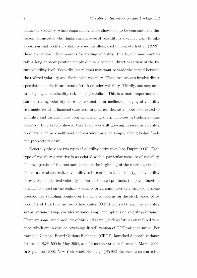
Figure 2.1: A comparison of fair strike values of actual-return variance swapsobtained from our closed-form solution, the continuous approximation and theMonte Carlo simulations, based on the Heston stochastic volatility model
where W 1t and W 2
t are two independent standard normal random variables.
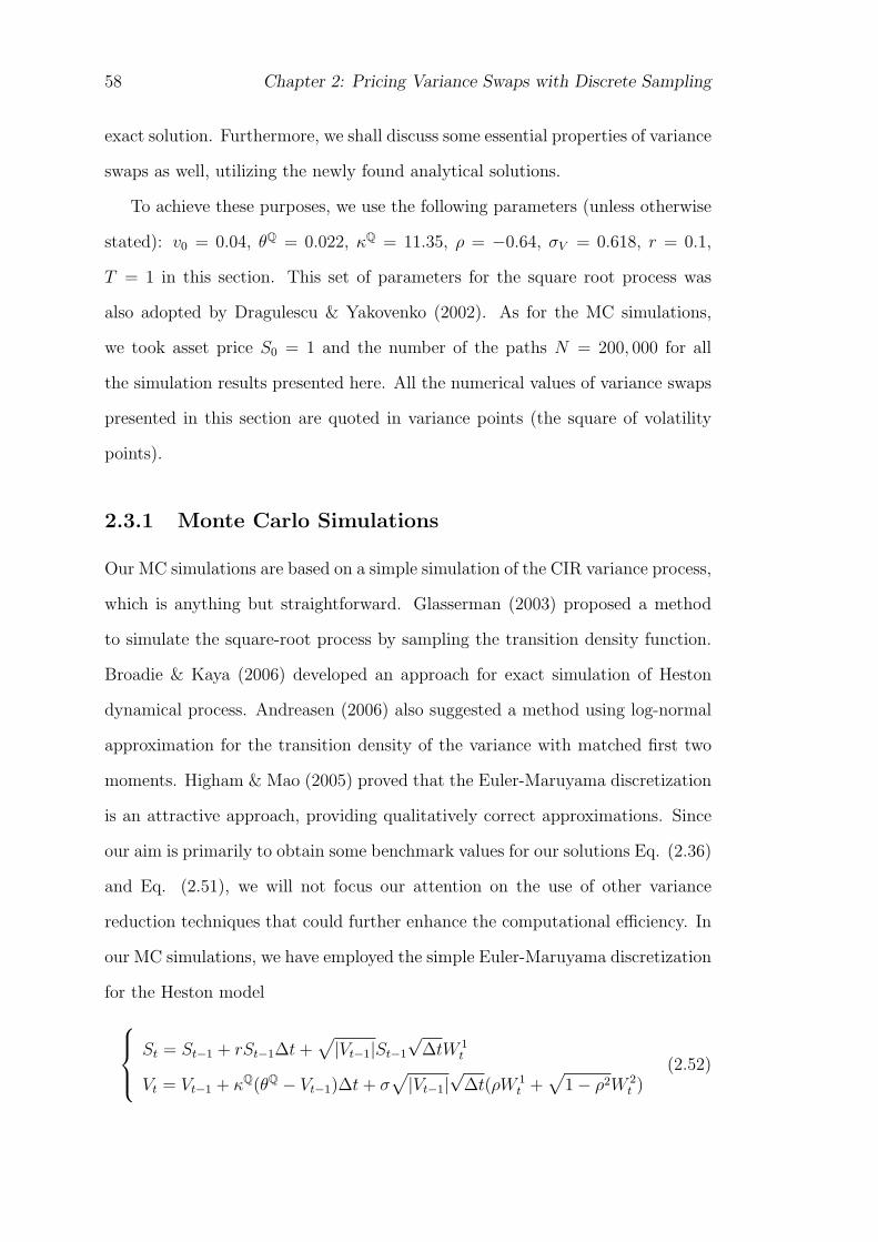
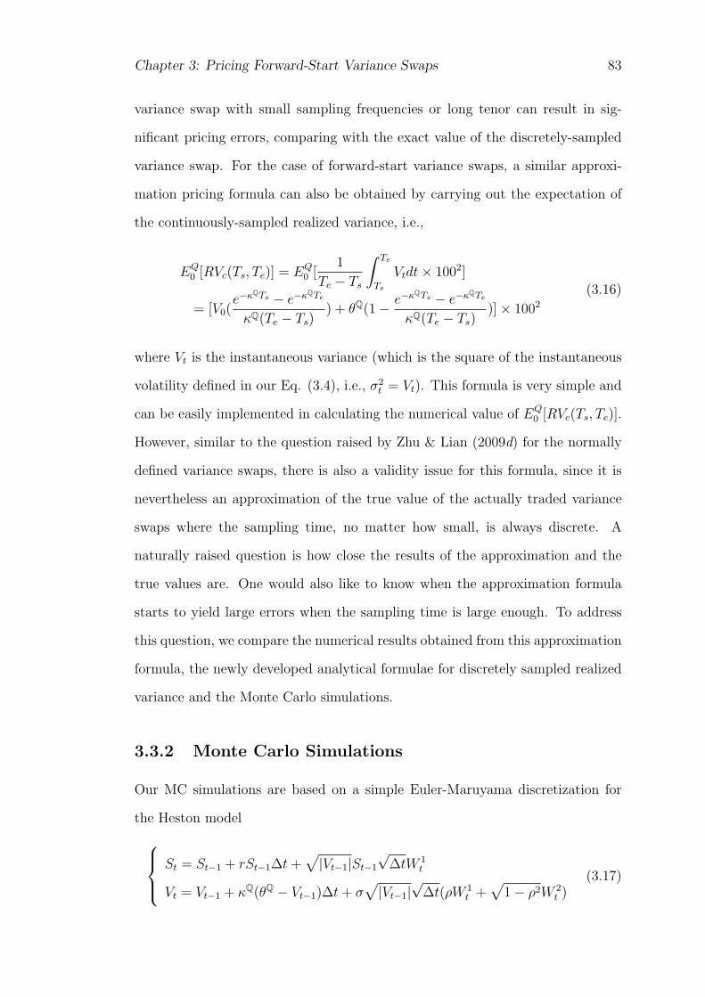
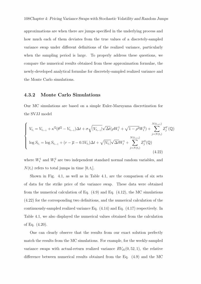
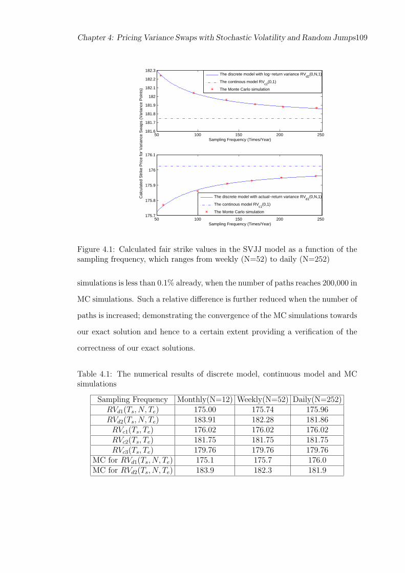
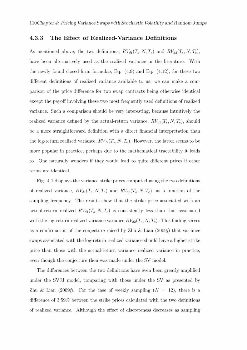
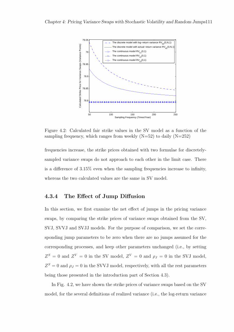
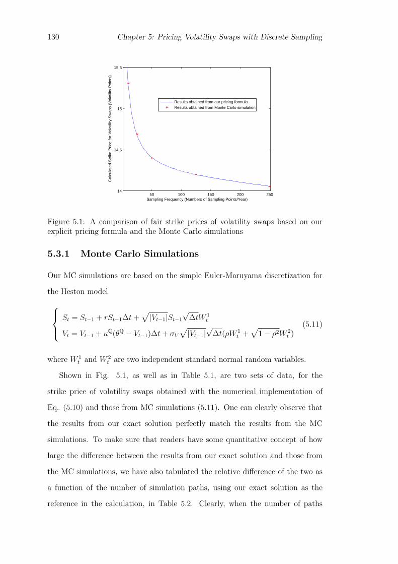
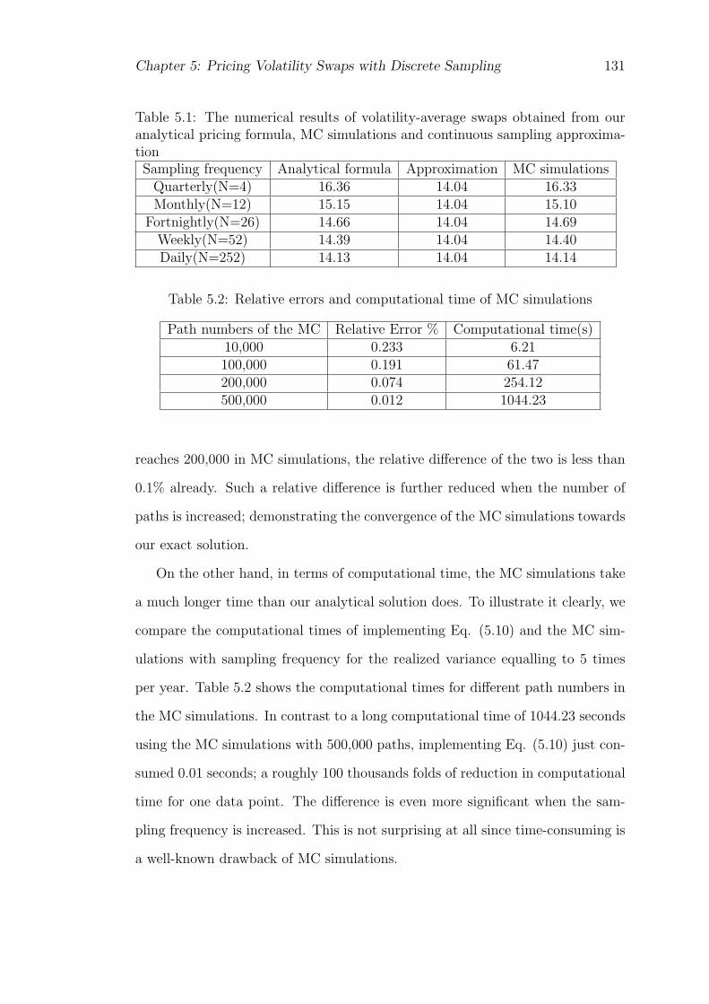
Shown in Fig. 2.1, as well as in Table 2.1, are three sets of data, for the
strike price of actual-return variance swaps obtained with the numerical imple-
mentation of Formula (2.36), those from MC simulations (2.52) and the numerical
results obtained from the continuously-sampled realized variance Formula (2.54).
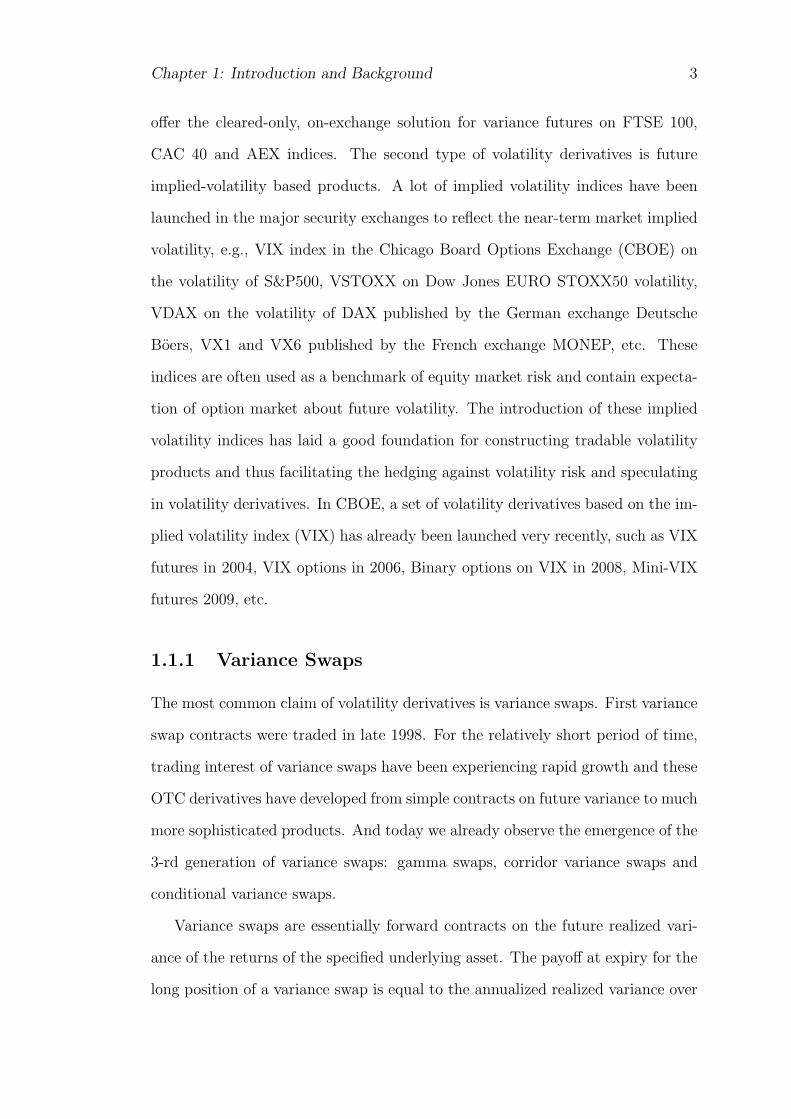
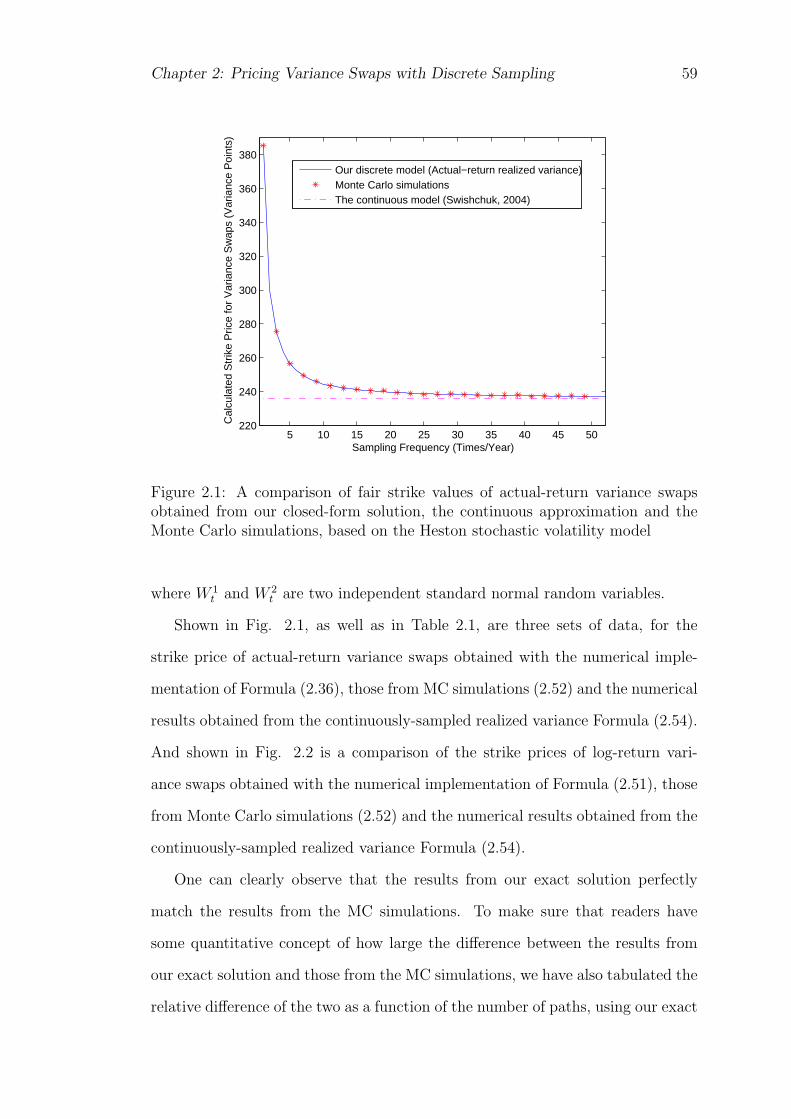
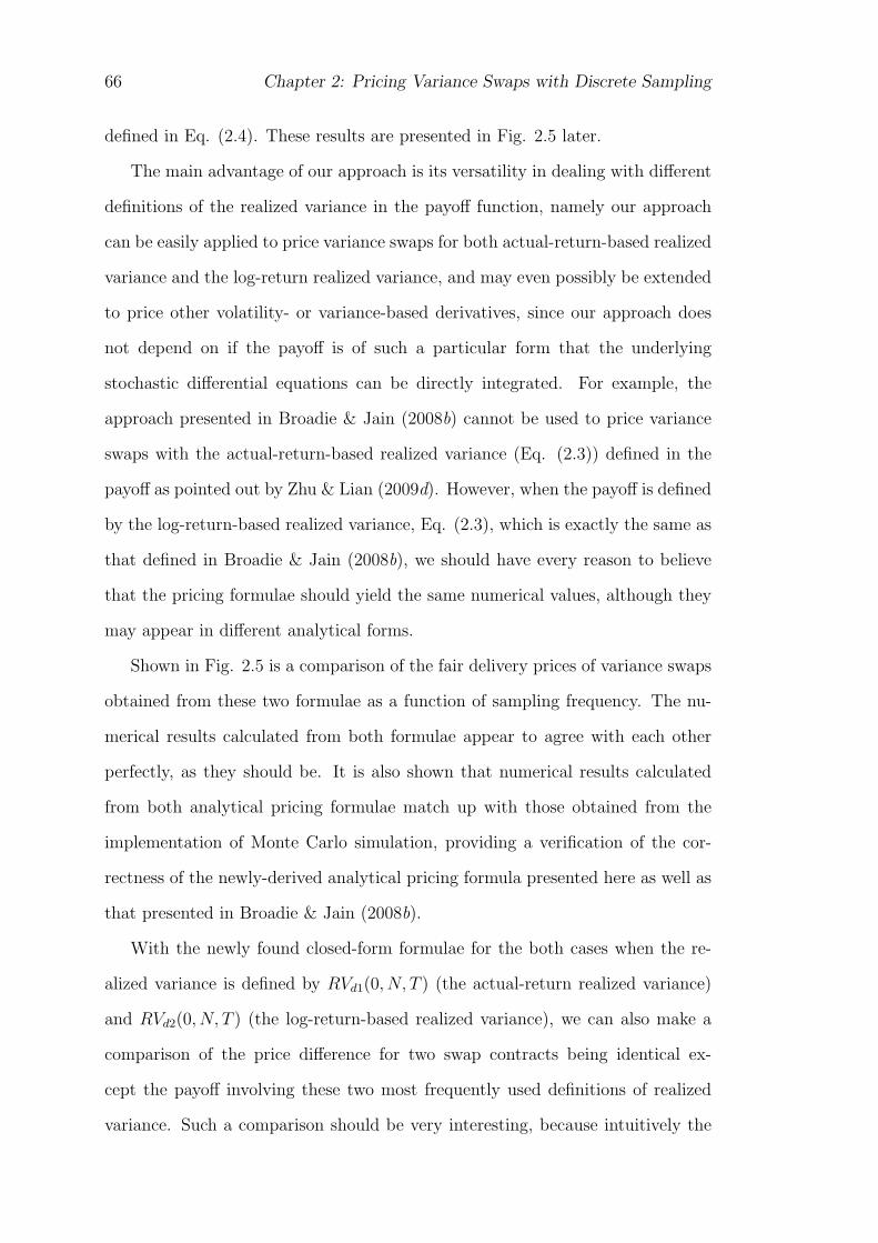
And shown in Fig. 2.2 is a comparison of the strike prices of log-return vari-
ance swaps obtained with the numerical implementation of Formula (2.51), those
from Monte Carlo simulations (2.52) and the numerical results obtained from the
continuously-sampled realized variance Formula (2.54).
One can clearly observe that the results from our exact solution perfectly
match the results from the MC simulations. To make sure that readers have
some quantitative concept of how large the difference between the results from
our exact solution and those from the MC simulations, we have also tabulated the
relative difference of the two as a function of the number of paths, using our exact
60 Chapter 2: Pricing Variance Swaps with Discrete Sampling
0 10 20 30 40 50
230
240
250
260
270
280
290
300
Sampling Frequency (Times/Year)
Cal
cula
ted
Str
ike
Pric
e fo
r V
aria
nce
Sw
aps
(Var
ianc
e P
oint
s)
Our discrete model (Log−return realized variance)Monte Carlo simulationsThe continuous model (Swishchuk, 2004)
Figure 2.2: A comparison of fair strike values of log-return variance swaps ob-tained from our closed-form solution, the continuous approximation and theMonte Carlo simulations, based on the Heston stochastic volatility model
solution (2.36) as the reference in the calculation, in Table 2.2. Clearly, when
the number of paths reaches 200,000 in MC simulations, the relative difference
of the two is less than 0.1% already. Such a relative difference is further reduced
when the number of paths is increased; demonstrating the convergence of the MC
simulations towards our exact solution.
On the other hand, in terms of computational time, the MC simulations take
a much longer time than our analytical solutions do. To illustrate it clearly,
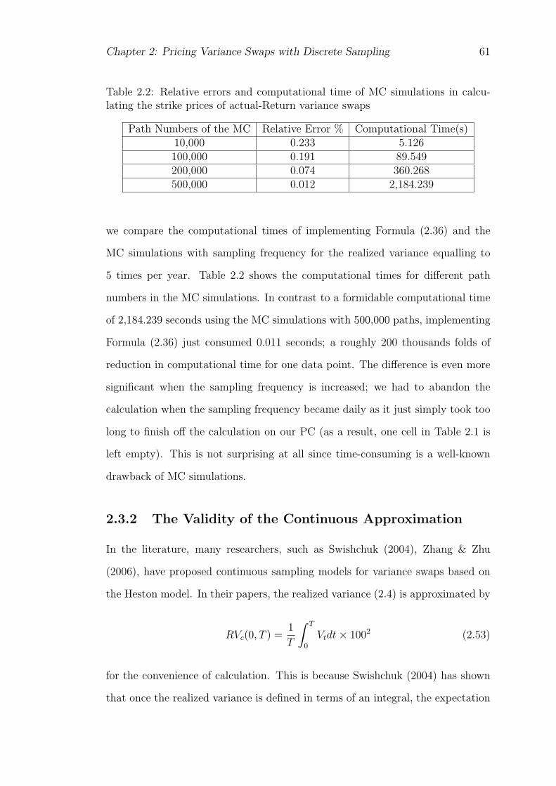
Table 2.1: The strike prices of discretely-sampled actual-return variance swapsobtained from our closed-form solution Eq. (2.36), the continuous approximationand MC simulations
Sampling Frequency Discrete Model Continuous Model MC SimulationsQuarterly(N=4) 267.6 235.9 267.3Monthly(N=12) 242.7 235.9 243.2
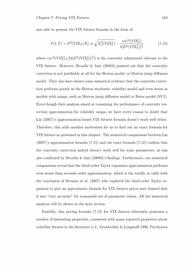
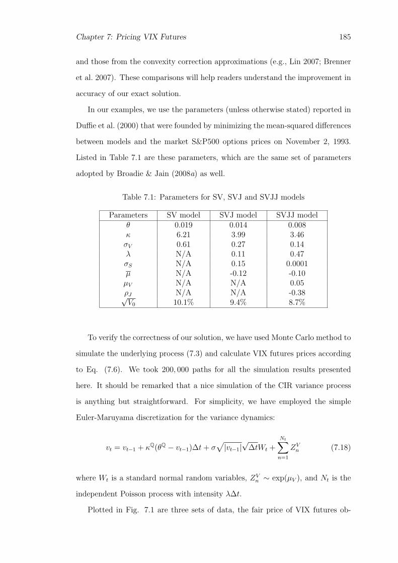
Chapter 2: Pricing Variance Swaps with Discrete Sampling 61
Table 2.2: Relative errors and computational time of MC simulations in calcu-lating the strike prices of actual-Return variance swaps
Path Numbers of the MC Relative Error % Computational Time(s)10,000 0.233 5.126100,000 0.191 89.549200,000 0.074 360.268500,000 0.012 2,184.239
we compare the computational times of implementing Formula (2.36) and the
MC simulations with sampling frequency for the realized variance equalling to
5 times per year. Table 2.2 shows the computational times for different path
numbers in the MC simulations. In contrast to a formidable computational time
of 2,184.239 seconds using the MC simulations with 500,000 paths, implementing
Formula (2.36) just consumed 0.011 seconds; a roughly 200 thousands folds of
reduction in computational time for one data point. The difference is even more
significant when the sampling frequency is increased; we had to abandon the
calculation when the sampling frequency became daily as it just simply took too
long to finish off the calculation on our PC (as a result, one cell in Table 2.1 is
left empty). This is not surprising at all since time-consuming is a well-known
drawback of MC simulations.
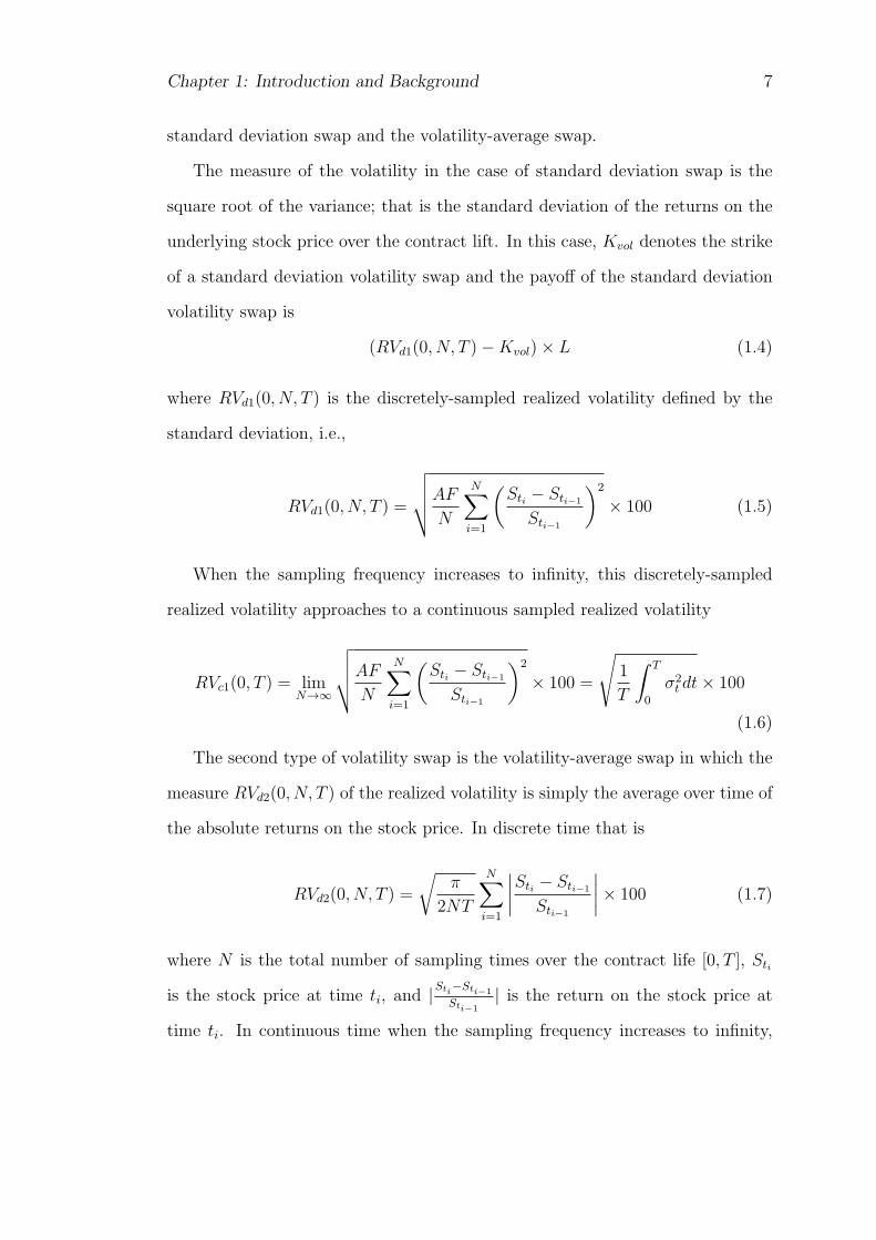
2.3.2 The Validity of the Continuous Approximation
In the literature, many researchers, such as Swishchuk (2004), Zhang & Zhu
(2006), have proposed continuous sampling models for variance swaps based on
the Heston model. In their papers, the realized variance (2.4) is approximated by
RVc(0, T ) =1
T
∫ T
0
Vtdt× 1002 (2.53)
for the convenience of calculation. This is because Swishchuk (2004) has shown
that once the realized variance is defined in terms of an integral, the expectation
62 Chapter 2: Pricing Variance Swaps with Discrete Sampling
of this continuous integral can be easily obtained, utilizing the second stochastic
process defined in (2.2). The resulting fair delivery price for the variance swap is
thus written as
EQ0 [RVc(0, T )] = [V0
1− e−κQT
κQT+ θQ(1− 1− e−κQT
κQT)]× 1002 (2.54)
which can be interpreted as a weighted average of the spot variance v0 and the
long-term mean of variance θQ. Indeed, this formula is very simple and can
be easily implemented in calculating the numerical value of EQ0 [RVc(0, T )]. For
the convenience of referencing, this formula will be referred to as the Swishchuk
formula hereafter, although many others also derived this formula.
Due to the lack of exact solution, in the past, for pricing a variance swap
with discrete sampling, the Swishchuk formula was primarily used in pricing
variance swaps, based on the assumption that the sampling period, such as daily
sampling, is short enough so that the result obtained from the continuous model
should be close to that without the continuum assumption of the sampling period.
However, no one knew exactly how close the results were because there was no
exact solution as a pricing formula for the case of discrete sampling times. Nor
did any one know when the Swishchuk formula starts to yield large errors when
the sampling time is large enough. In other words, there is a validity issue for
the Swishchuk formula, since it is nevertheless an approximation in the trading
practice where the sampling time, no matter how small, is always discrete. Our
newly-derived formulae can now be used not only as pricing formulae for any
discrete sample period, but also as a validation tool for checking the accuracy
level that the Swishchuk formula yields as a function of the sampling period.
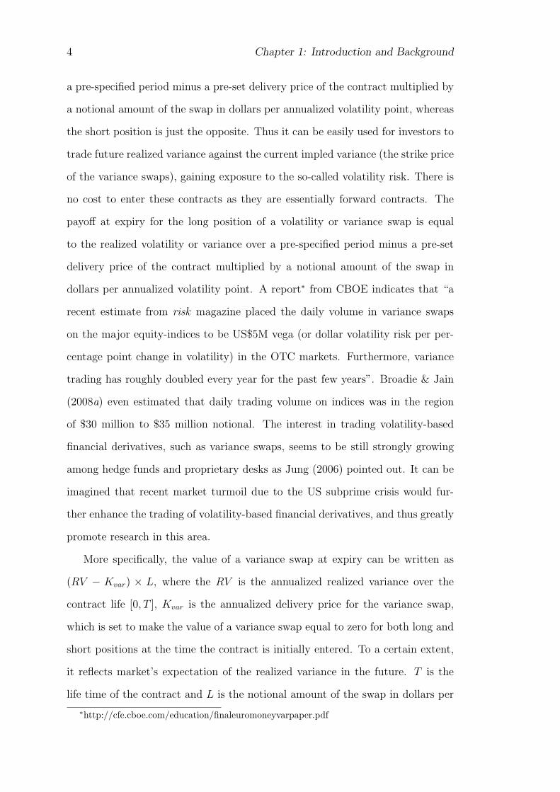
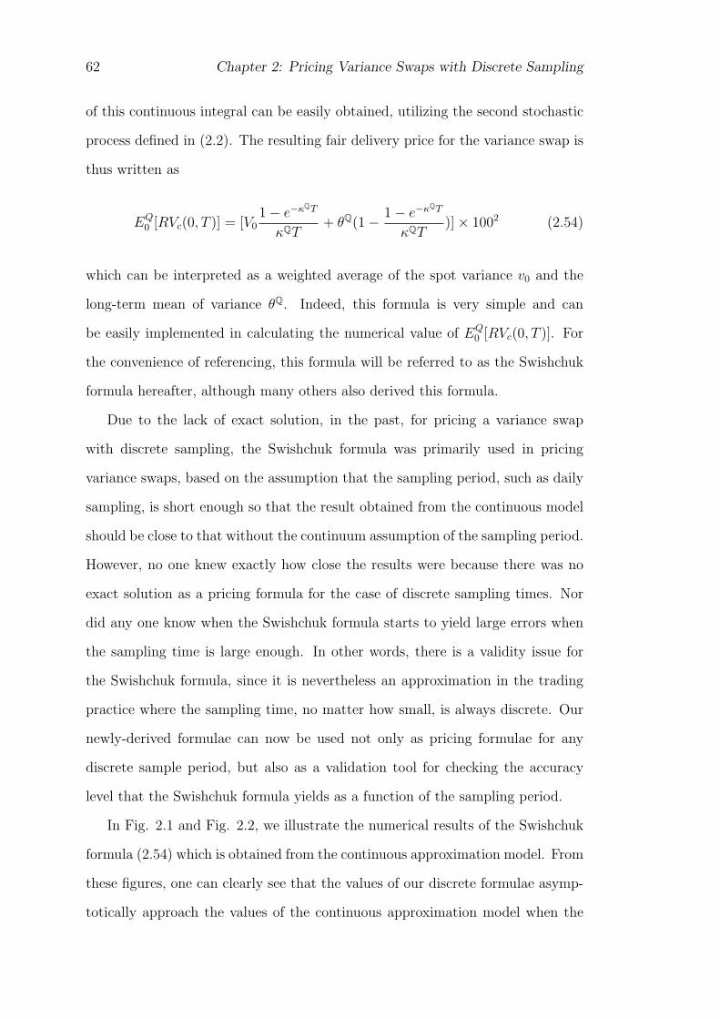
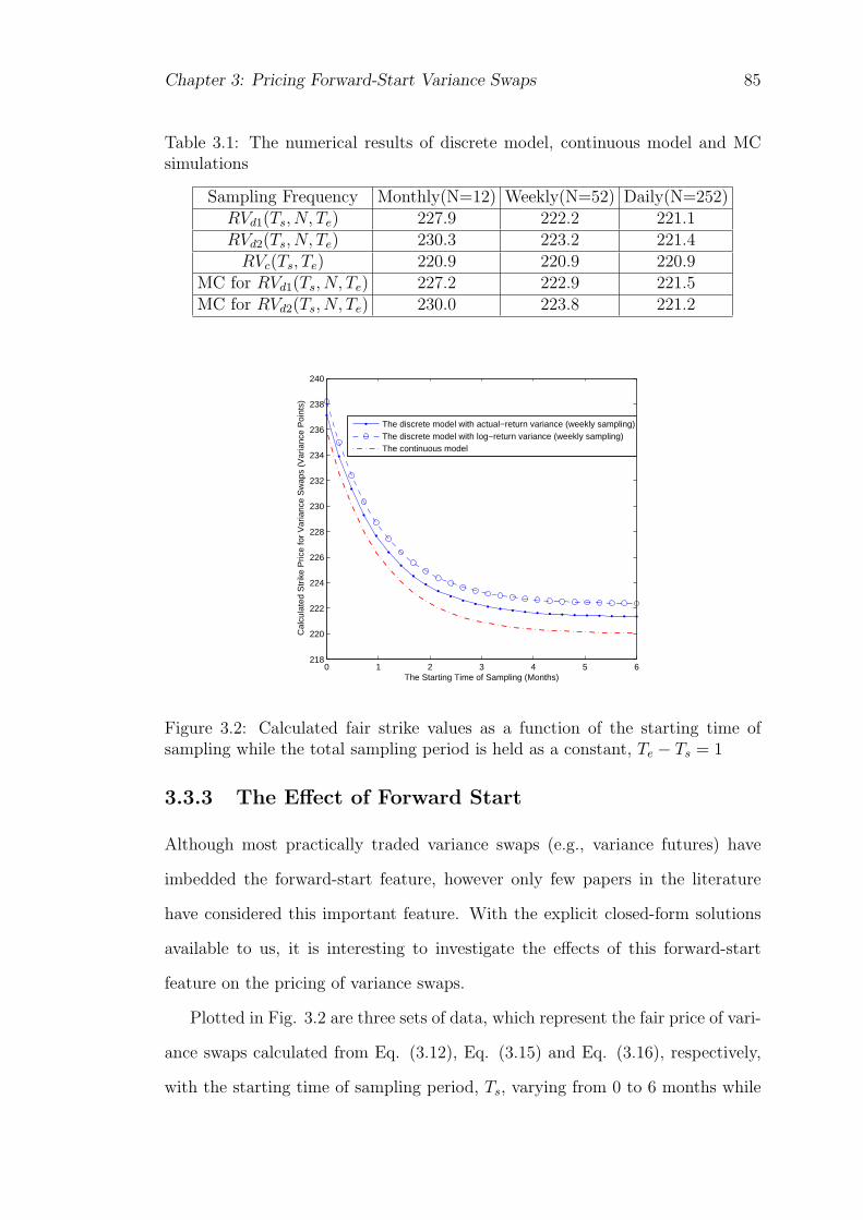
In Fig. 2.1 and Fig. 2.2, we illustrate the numerical results of the Swishchuk
formula (2.54) which is obtained from the continuous approximation model. From
these figures, one can clearly see that the values of our discrete formulae asymp-
totically approach the values of the continuous approximation model when the
Chapter 2: Pricing Variance Swaps with Discrete Sampling 63
50 100 150 200 250235
235.5
236
236.5
237
237.5
238
238.5
239
239.5
240
Sampling Frequency (Times/Year)
Cal
cula
ted
Str
ike
Pric
e fo
r V
aria
nce
Sw
aps
(Var
ianc
e P
oint
s)
Strike prices based on log−return realized varianceStrike prices based on Swishchuk (2004) formulaStrike prices based on actual−return realized variance
Figure 2.3: Calculated fair strike values of actual-return and log-return varianceswaps as a function of sampling frequency
sampling frequency increases; the realized variance defined in (2.53) appears to
be the limit of the realized variance defined in Eq. (2.4) and Eq. (2.3) as ∆t→ 0.
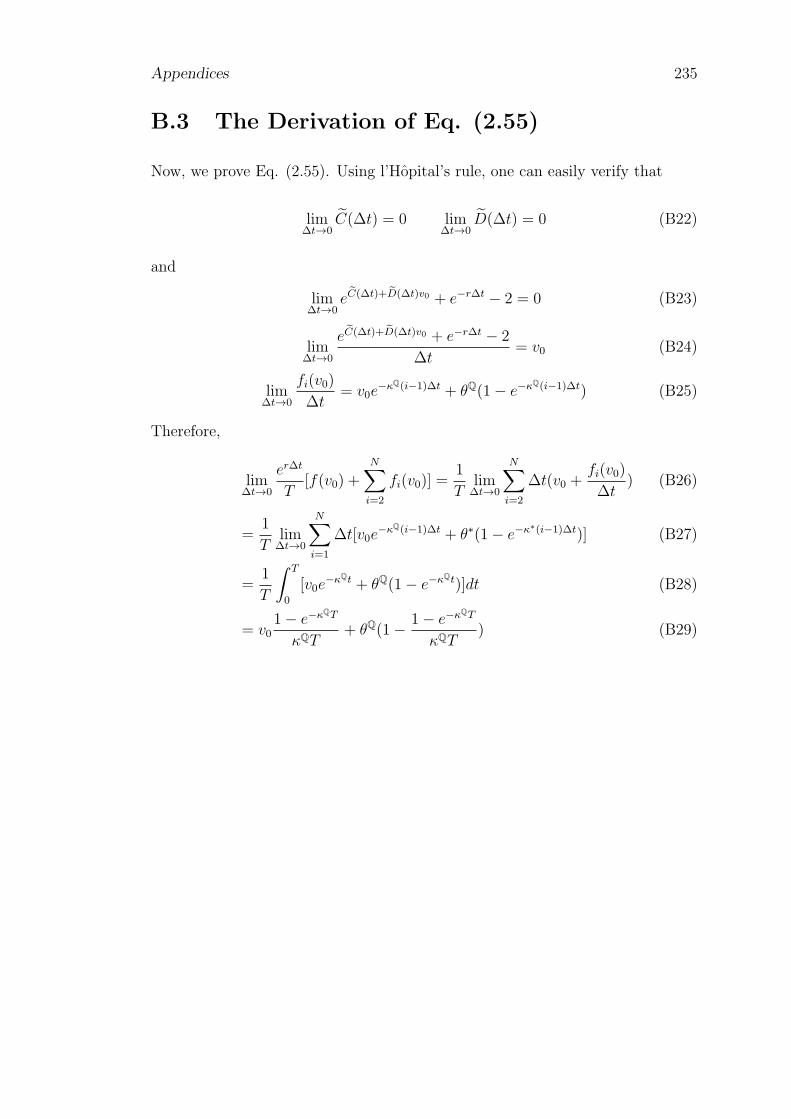
Of course, one can theoretically prove that our solutions (2.36) and (2.51) indeed
approach the Formula (2.54) when the discrete sampling period approaches zero,
i.e.,
lim∆t→0
er∆t
T[f(V0) +
N∑i=2
fi(V0)] = V01− e−κQT
κQT+ θQ(1− 1− e−κQT
κQT) (2.55)
With the proof of this limit, which is left in Appendix B.3, our solution is once
again verified as the correct solution for the discrete sampling cases, taking the
continuous sampling case as a special case with the sampling period shrinking
down to zero.
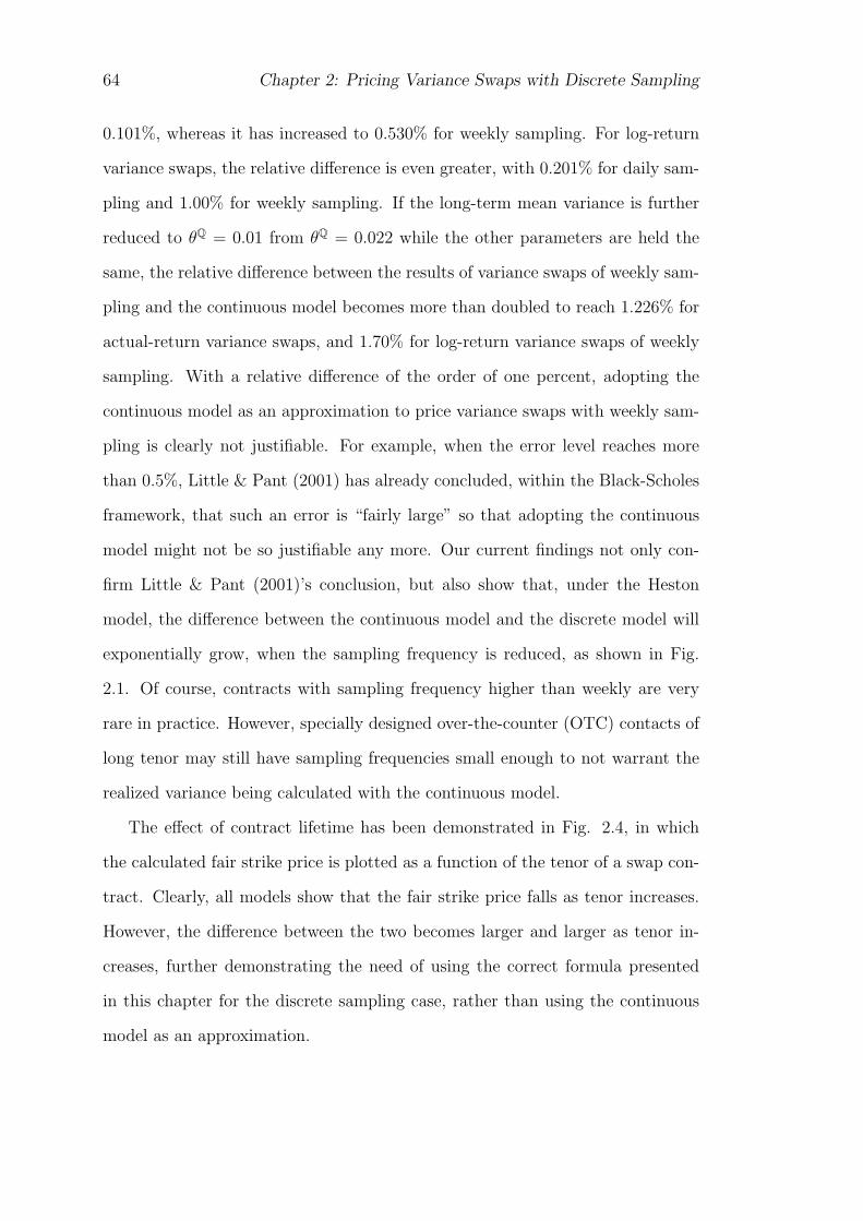
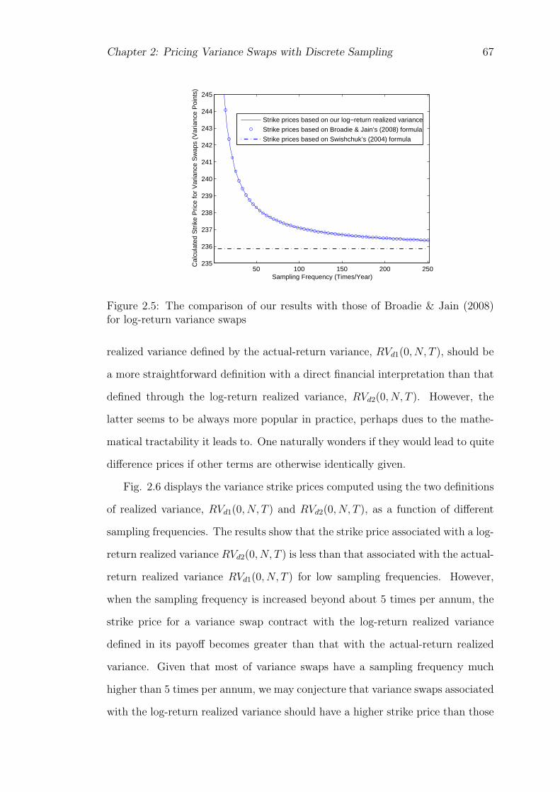
On the other hand, we now can use our discrete model to check the validity of
the continuous model as an approximation. Shown in Fig. 2.3 is a refined plot of
Fig. 2.1 and Fig. 2.2, in order to compare the degree of approximation between
daily and weekly sampling. With the daily sampling, the relative difference be-
tween the results of the actual-return variance swap and the continuous model is
64 Chapter 2: Pricing Variance Swaps with Discrete Sampling
0.101%, whereas it has increased to 0.530% for weekly sampling. For log-return
variance swaps, the relative difference is even greater, with 0.201% for daily sam-
pling and 1.00% for weekly sampling. If the long-term mean variance is further
reduced to θQ = 0.01 from θQ = 0.022 while the other parameters are held the
same, the relative difference between the results of variance swaps of weekly sam-
pling and the continuous model becomes more than doubled to reach 1.226% for
actual-return variance swaps, and 1.70% for log-return variance swaps of weekly
sampling. With a relative difference of the order of one percent, adopting the
continuous model as an approximation to price variance swaps with weekly sam-
pling is clearly not justifiable. For example, when the error level reaches more
than 0.5%, Little & Pant (2001) has already concluded, within the Black-Scholes
framework, that such an error is “fairly large” so that adopting the continuous
model might not be so justifiable any more. Our current findings not only con-
firm Little & Pant (2001)’s conclusion, but also show that, under the Heston
model, the difference between the continuous model and the discrete model will
exponentially grow, when the sampling frequency is reduced, as shown in Fig.
2.1. Of course, contracts with sampling frequency higher than weekly are very
rare in practice. However, specially designed over-the-counter (OTC) contacts of
long tenor may still have sampling frequencies small enough to not warrant the
realized variance being calculated with the continuous model.
The effect of contract lifetime has been demonstrated in Fig. 2.4, in which
the calculated fair strike price is plotted as a function of the tenor of a swap con-
tract. Clearly, all models show that the fair strike price falls as tenor increases.
However, the difference between the two becomes larger and larger as tenor in-
creases, further demonstrating the need of using the correct formula presented
in this chapter for the discrete sampling case, rather than using the continuous
model as an approximation.
Chapter 2: Pricing Variance Swaps with Discrete Sampling 65
1 2 3 4 5 6 7 8 9 10220
222
224
226
228
230
232
234
236
238
240
Tenor of Variance Swaps (Years, weekly sampling for discrete models)
Cal
cula
ted
Str
ike
Pric
e fo
r V
aria
nce
Sw
aps
(Var
ianc
e P
oint
s)
Strike prices based on log−return realized varianceStrike prices based on actual−return realized varianceStrike prices based on Swishchuk (2004) formula
Figure 2.4: Calculated fair strike values of actual-return and log-return varianceswaps as a function of tenor
2.3.3 Comparison with Other Solutions
Recently, Broadie & Jain (2008b) presented a closed-form formula for log-return
variance swaps as that presented in this chapter. However, their solution approach
is totally different from ours as what we have presented here. While Broadie &
Jain (2008b) derived the discrete variance strike for variance swaps by integrating
the underlying stochastic processes directly, we have directly solved the governing
PDEs that were derived based on the same underlying stochastic processes. The
two resulting formulae appear to be quite different in form. It is therefore quite
interesting to compare the prices of discretely-sampled variance swaps obtained
from these two formulae.
One should notice that the definition of the realized variance defined in Broadie
& Jain (2008b) is slightly different from Eq. (2.4) used in this thesis. However,
the difference between the two is so trivial that all we needed to do was to re-scale
the calculated results by a constant, in order to make a good comparison with the
results presented in Broadie & Jain (2008b). In other words, the results we have
re-calculated from Broadie & Jain (2008b)’s formula were obtained with their Eq.
(45) being re-scaled by a factor of N−1N
, where N is the number of sampling points
66 Chapter 2: Pricing Variance Swaps with Discrete Sampling
defined in Eq. (2.4). These results are presented in Fig. 2.5 later.
The main advantage of our approach is its versatility in dealing with different
definitions of the realized variance in the payoff function, namely our approach
can be easily applied to price variance swaps for both actual-return-based realized
variance and the log-return realized variance, and may even possibly be extended
to price other volatility- or variance-based derivatives, since our approach does
not depend on if the payoff is of such a particular form that the underlying
stochastic differential equations can be directly integrated. For example, the
approach presented in Broadie & Jain (2008b) cannot be used to price variance
swaps with the actual-return-based realized variance (Eq. (2.3)) defined in the
payoff as pointed out by Zhu & Lian (2009d). However, when the payoff is defined
by the log-return-based realized variance, Eq. (2.3), which is exactly the same as
that defined in Broadie & Jain (2008b), we should have every reason to believe
that the pricing formulae should yield the same numerical values, although they
may appear in different analytical forms.
Shown in Fig. 2.5 is a comparison of the fair delivery prices of variance swaps
obtained from these two formulae as a function of sampling frequency. The nu-
merical results calculated from both formulae appear to agree with each other
perfectly, as they should be. It is also shown that numerical results calculated
from both analytical pricing formulae match up with those obtained from the
implementation of Monte Carlo simulation, providing a verification of the cor-
rectness of the newly-derived analytical pricing formula presented here as well as
that presented in Broadie & Jain (2008b).
With the newly found closed-form formulae for the both cases when the re-
alized variance is defined by RVd1(0, N, T ) (the actual-return realized variance)
and RVd2(0, N, T ) (the log-return-based realized variance), we can also make a
comparison of the price difference for two swap contracts being identical ex-
cept the payoff involving these two most frequently used definitions of realized
variance. Such a comparison should be very interesting, because intuitively the
Chapter 2: Pricing Variance Swaps with Discrete Sampling 67
50 100 150 200 250235
236
237
238
239
240
241
242
243
244
245
Sampling Frequency (Times/Year)
Cal
cula
ted
Str
ike
Pric
e fo
r V
aria
nce
Sw
aps
(Var
ianc
e P
oint
s)
Strike prices based on our log−return realized variance
Strike prices based on Broadie & Jain’s (2008) formula
Strike prices based on Swishchuk’s (2004) formula
Figure 2.5: The comparison of our results with those of Broadie & Jain (2008)for log-return variance swaps
realized variance defined by the actual-return variance, RVd1(0, N, T ), should be
a more straightforward definition with a direct financial interpretation than that
defined through the log-return realized variance, RVd2(0, N, T ). However, the
latter seems to be always more popular in practice, perhaps dues to the mathe-
matical tractability it leads to. One naturally wonders if they would lead to quite
difference prices if other terms are otherwise identically given.
Fig. 2.6 displays the variance strike prices computed using the two definitions
of realized variance, RVd1(0, N, T ) and RVd2(0, N, T ), as a function of different
sampling frequencies. The results show that the strike price associated with a log-
return realized variance RVd2(0, N, T ) is less than that associated with the actual-
return realized variance RVd1(0, N, T ) for low sampling frequencies. However,
when the sampling frequency is increased beyond about 5 times per annum, the
strike price for a variance swap contract with the log-return realized variance
defined in its payoff becomes greater than that with the actual-return realized
variance. Given that most of variance swaps have a sampling frequency much
higher than 5 times per annum, we may conjecture that variance swaps associated
with the log-return realized variance should have a higher strike price than those
68 Chapter 2: Pricing Variance Swaps with Discrete Sampling
with the actual-return variance realized variance in practice. The reason that
we call this a conjecture rather than a conclusion is that to draw a conclusion,
one really needs to test if this is true for all other parameters in the parameter
space. Such tests must be thorough, and thus would be quite time consuming.
Therefore, we have decided to leave it for future research. On the other hand, our
conjecture is indeed reenforced by the results presented in Fig. 2.3 and Fig. 2.4,
which further demonstrate that both strike prices associated with the log-return
realized variance and the actual-return variance realized variance are higher than
those associated with the continuously-sampling approximation, but strike prices
associated with the log-return is usually higher than those associated with the
actual return, at least for the most common sampling frequencies used in financial
practice. In practice most of the contracts sampling is done daily or weekly and
sometimes monthly (very rarely). For weekly sampling realized variance, there is
a 0.46% difference between the strike prices calculated with the two definitions
of realized variance. The effect of discreteness further decreases as sampling
frequencies increases further; the strike prices obtained with two formulae for
discretely-sampled variance swaps do approach to that of the continuous-sampled
variance swaps, as one would have expected.
A couple of more points should be remarked before leaving this section.
Firstly, with the newly found analytic solution, all the hedging ratios of a variance
swap can also be analytically derived by taking partial derivatives against various
parameters in the model. With symbolic calculation packages, such Mathematica
or Maple, widely available to researchers and market practitioners, these partial
derivatives can be readily calculated and thus omitted here. However, to demon-
strate how sensitive the strike price is to the change of the key parameters in
the model, we performed some sensitivity tests for the example presented in this
section. Shown in Table 2.3 are the results of the percentage change of the strike
price when a model parameter is given a 1% change from its base value used in
the example presented in this Section. Clearly, the strike price of a variance swap
Chapter 2: Pricing Variance Swaps with Discrete Sampling 69
5 10 15 20 25 30 35 40 45 50220
230
240
250
260
270
280
290
300
Sampling Frequency (Times/Years)
Cal
cula
ted
Str
ike
Pric
e fo
r V
aria
nce
Sw
aps
(Var
ianc
e P
oint
s)
Strike prices based on log−return realized varianceStrike prices based on actual−return realized varianceStrike prices based on Swishchuk’s (2004) formula
Figure 2.6: The effect of alternative measures of realized variance
appears to be most sensible to the long-term mean variance θQ for the case stud-
ied. On the other hand, the spot variance V0 may also have significant influence
in terms of the sensitivity of the strike price. Secondly, due to the notational
amount factor L and the size of the contract traded per order, the 1% or 2%
relative error may result in a considerable amount of absolute loss if the formula
based on the continuous approximation is adopted. Combining these two points
together, one may conclude that even with a relatively high sampling frequency,
such as daily sampling, the approximation based on the continuous model could
still lead to larger errors for a certain combination of parameter values. Thereby,
having closed-form formulae for the case of discrete sampling would enable us to
completely abandon the approximation formula based on the continuous model;
whether the sampling period is small or not, the computational time of adopting
our newly-derived formulae, Eq. (2.36), and Eq. (2.51) is virtually the same as
that of adopting the traditional formula, Eq. (2.54).
70 Chapter 2: Pricing Variance Swaps with Discrete Sampling
Table 2.3: The sensitivity of strike price of variance swap (daily sampling)
Name Value SensitivityκQ 11.35 -0.066%θQ 0.022 0.85%σV 0.618 -0.0015%V0 0.04 0.15%
2.4 Conclusion
In this chapter, we have applied the Heston stochastic volatility model to describe
the underlying asset price and its volatility, and obtained two closed-form exact
solutions for discretely-sampled variance swaps with the actual-return and log-
return realized variance. This can be viewed as a substantial progress made in
developing a more realistic pricing model for variance swaps. Through numerical
examples, we have shown that the our formulae can improve the accuracy in
pricing variance swaps. We have compared the results produced from our new
solutions with those produced by the MC simulations for the validation purposes
and found that our results agree with those from the MC simulations perfectly.
The significance of our work can be illustrated in two aspects. Theoretically,
our discrete model can be used to verify the validity of the corresponding con-
tinuous models. Our study has demonstrated that the well-known continuous
approximation in the literature for variance swaps leads to an error exponentially
growing with the inverse of the sampling frequencies. The study of this chapter
thus would fill a gap that has been in the field of pricing variance swaps. Fourier
inverse transform in our model has been analytically worked out, which is a
significant step forward in the literature of Heston’s model. Practically, the com-
putational efficiency is enormously enhanced in terms of assisting practitioners
to price variance swaps, and thus it can be a very useful tool in trading practice
when there is obviously increasing demand of trading variance swaps in financial
markets.
Chapter 3
Pricing Forward-Start Variance
Swaps
3.1 Introduction
In Chapter 2, we have discussed the pricing of discretely-sampled variance swaps,
based on the Heston stochastic volatility model, to improve the pricing accuracy
the continuously-sampling approximations in literature. This chapter will address
the pricing problem of forward-start variance swaps, as most of those traded
variance swaps in markets or even some over-the-counter ones are of a forward-
start nature, characterized by the starting time of the sampling period being a
future date.
Forward-start variance swaps are a kind of variance swaps whose annual-
ized realized variance is measured between two future dates Ts and Te, where
0 < Ts < Te, with t = 0 being the current time. Even though forward-start vari-
ance swaps seem to be a simple and natural extension to the normally defined
variance swaps with the sampling period covering all the time between now and a
future time T , the introduction of the forward-start feature can increase the flex-
ibility of variance swaps in hedging risk, and hence greatly promote the trading
of variance swaps. This is indeed the case as variance futures are indeed listed as
The discrete model with actual−return varianceThe discrete model with log−return varianceThe continuous modelThe MC simulation with actual−return varianceThe MC simulation with log−return variance
Figure 3.1: Calculated fair strike values as a function of sampling frequency
where W 1t and W 2
t are two independent standard normal random variables.
Shown in Fig. 3.1, as well as in Table 3.1, are the comparison of five sets of
data for the strike price of the variance swap. These data were obtained from
the numerical calculation of Eq. (3.12) and Eq. (3.15), the MC simulations
(3.17) for the corresponding two definitions, and the numerical calculation of
the continuously-sampled realized variance Eq. (3.16), respectively. The starting
time of the sampling period is set to be 3 months (i.e., Ts = 1/3) in the calculation
of the forward-start variance swaps. One can clearly observe that the results
from our exact solution perfectly match the results from the MC simulations. For
example, for the forward-start variance swaps with actual-return realized variance
RVd1(Ts, N, Te), the relative difference between numerical results obtained from
the Eq. (3.12) and the MC simulations is less than 0.1% already, when the number
of paths reaches 200,000 in MC simulations. Such a relative difference is further
reduced when the number of paths is increased; demonstrating the convergence
of the MC simulations towards our exact solution and hence to a certain extent
providing a verification of the correctness of our exact solutions.
Table 3.1: The numerical results of discrete model, continuous model and MCsimulations
Sampling Frequency Monthly(N=12) Weekly(N=52) Daily(N=252)RVd1(Ts, N, Te) 227.9 222.2 221.1RVd2(Ts, N, Te) 230.3 223.2 221.4RVc(Ts, Te) 220.9 220.9 220.9
MC for RVd1(Ts, N, Te) 227.2 222.9 221.5MC for RVd2(Ts, N, Te) 230.0 223.8 221.2
0 1 2 3 4 5 6218
220
222
224
226
228
230
232
234
236
238
240
The Starting Time of Sampling (Months)
Cal
cula
ted
Str
ike
Pric
e fo
r V
aria
nce
Sw
aps
(Var
ianc
e P
oint
s)
The discrete model with actual−return variance (weekly sampling)The discrete model with log−return variance (weekly sampling)The continuous model
Figure 3.2: Calculated fair strike values as a function of the starting time ofsampling while the total sampling period is held as a constant, Te − Ts = 1
3.3.3 The Effect of Forward Start
Although most practically traded variance swaps (e.g., variance futures) have
imbedded the forward-start feature, however only few papers in the literature
have considered this important feature. With the explicit closed-form solutions
available to us, it is interesting to investigate the effects of this forward-start
feature on the pricing of variance swaps.
Plotted in Fig. 3.2 are three sets of data, which represent the fair price of vari-
ance swaps calculated from Eq. (3.12), Eq. (3.15) and Eq. (3.16), respectively,
with the starting time of sampling period, Ts, varying from 0 to 6 months while
The discrete model with actual−return variance (weekly sampling)The discrete model with log−return variance (weekly sampling)The continuous model
Figure 3.3: Calculated fair strike values as a function of the starting time ofsampling while the terminating time of sampling is held as a constant, Te = 1
width of the sampling window Te − Ts now varies with the change of the start of
the sampling Ts. But, the trend displayed in Fig. 3.3 appears to be very similar
to that displayed in Fig. 3.2. Therefore, we can conclude that if the start of the
sampling time is too far away from the current time, one may use the long-term
mean of variance as a good approximation for the expectation of the realized
variance, regardless of the width of the sampling window Te − Ts being a fixed
constant or not.
3.3.4 The Effect of Mean-reverting Speed
κQ is the parameter controlling the speed of mean reversion from the spot vari-
ance. Again, using the continuous sampling case, one can easily understand how
κQ controls the speed of mean reversion towards the long-term mean of variance.
From Eq. (3.16), we can see that WV0 is a decreasing function of the parameter
κQ, which means a greater value of κQ reduces the weight of V0 on the total value
of variance swap, while increasing the weight of θQ at the same time. Therefore,
a higher value of κQ means the variance Vt approaches to the long-term mean of
The discrete model with actual−return variance (weekly sampling)The discrete model with log−return variance (weekly sampling)
kappa=5
kappa=11.35
Figure 3.4: Calculated fair strike values as a function of the starting time ofsampling while the total sampling period is held as a constant, Te − Ts = 1
variance θQ more quickly, and as a result, θQ naturally gains more weight on the
value of the variance swap.
Demonstrated in Fig. 3.4 is the effect of κ on the prices of variance swaps.
When κ is specified to be 11.35, the value of a 3-month forward-start variance
swap (Ts = 3/12) is 222 forRVd1(3/12, 52, 15/12) and 223 forRVd2(3/12, 52, 15/12),
respectively; whereas, when κQ is reduced to be 5 and other parameters are holden
the same, the value of a 3-month forward-start variance swap increases to be 231
and 232 for the two corresponding definitions of the realized variance. One should
also notice that the value of forward-start variance swap with a larger κQ value
is consistently lower than that with smaller κQ. This is because a larger κQ value
has made θQ being weighted much more than V0, although the former is specified
smaller than latter in this example, resulting a lower price of variance swap for
all the starting time that has been examined and displayed in Fig. 3.4. If the
specification of θQ and V0 is reversed, i.e., with θQ > V0, the prices of variance
swaps with different κQ values should be reversed too.
λ = 0.47, µV = 0.05, µS = −0.086∗, σS = 0.0001, ρJ = −0.38, r = 3.19%. This
set of parameters was also adopted by Broadie & Jain (2008a). As for the MC
simulations, we took asset price S0 = 1 and the number of the paths N = 500, 000
for all the simulation results presented here. Following the quotation rules of
variance futures in CBOE, all the numerical values of variance swaps presented
in this section are quoted in terms of variance points (the square of volatility
points), which are defined as realized variance multiplied by 10,000.
4.3.1 Continuous Sampling Approximation
Before performing the Monte Carlo simulations, we have also worked out the
corresponding pricing formula based on the continuous sampling approximation,
under the framework of SVJJ model.
In the literature, many researchers (i.e., Swishchuk 2004) have proposed con-
tinuous sampling approximations for realized variance to price the variance swaps,
based on the Heston stochastic volatility model. Some others (e.g., Little & Pant
∗The value of µS is backward calculated by using µ = θ(1, 0) − 1 with µ = −0.10 in Duffieet al. (2000).
Chapter 4: Pricing Variance Swaps with Stochastic Volatility and Random Jumps105
2001, Broadie & Jain 2008b, Zhu & Lian 2009d,f) however pointed out that adopt-
ing such a continuous sampling approximation under the SV model for a variance
swap with small sampling frequencies or long tenor can result in significant pric-
ing errors, comparing with the exact value of the discretely-sampled variance
swap. As for the framework of SVJJ model, the continuous sampling approxima-
tions become somewhat more complicate, due to the fact that there exist several
versions of continuously-sampled realized variance.
Corresponding to the definition of actual-return realized variance, Eq. (3.2),
the continuously-sampled realized variance is denoted by the RVc1(Ts, Te) and
given by:
RVc1(Ts, Te) = limN→∞
AF
N
N∑i=1
(Sti − Sti−1
Sti−1
)2
× 1002
=
1
Te − Ts
∫ Te
Ts
Vtdt+
N(Te)∑k=N(Ts)
(eZsk − 1)2
× 1002(4.13)
The expectation of this expression can be carried out and hence the approximation
pricing formula for a variance swap based on this continuously-sampled realized
variance is obtained,
EQ0 [RVc1(Ts, Te)] = [AV0 + (1− A)(θQ +
λµV
κQ) + λC1]× 1002 (4.14)
with
A =e−κQTs − e−κQTe
κQ(Te − Ts)
C1 =exp(2µS + 2σ2
S)
1− 2ρJµV
− 2exp(µS +
σ2S
2)
1− ρJµV
+ 1
(4.15)
Zhu & Lian (2009f) presented numerical examples based on the SV model to
demonstrate that the prices of variance swaps obtained from the two discretely-
sampled variance swaps asymptotically approach to the value of continuous-
sampled variance swaps when the sampling frequency increases to infinity. Their
work shows that the effect of discreteness resulted from the different definition of
discretely-sampled realized variance decreases as sampling frequencies increases
106Chapter 4: Pricing Variance Swaps with Stochastic Volatility and Random Jumps
and the two definitions of discretely-sampled realized variance have the same
limiting value when the discrete sampling time approaches zero. Under the
SVJJ model, however, the continuous sampling approximations for the discretely-
sampled actual-return or log-return realized variance (i.e., the limiting value of
Eq. (3.2) and Eq. (3.3) when the sampling frequency increases to infinity) are
not the same any more. We used the RVc2(Ts, Te) to denote the continuously-
sampled realized variance corresponding to the log-return realized variance, Eq.
(3.3), i.e.,
RVc2(Ts, Te) = limN→∞
AF
N
N∑i=1
log2(Sti
Sti−1
)× 1002
=
1
Te − Ts
∫ Te
Ts
Vtdt+
N(Te)∑k=N(Ts)
(Zsk)
2
× 1002(4.16)
The expectation of this expression can also be carried out and the approximation
pricing formula for a variance swap based on this continuously-sampled realized
variance is obtained as,
EQ0 [RVc2(Ts, Te)] = [AV0 + (1− A)(θQ +
λµV
κQ) + λC2]× 1002 (4.17)
with
A =e−κQTs − e−κQTe
κQ(Te − Ts)
C2 = σ2S + 2ρ2Jµ
2V + 2ρJµV µS + µ2
S
(4.18)
These two versions (i.e., Eq. (4.14) and Eq. (4.17)) of continuously-sampled
realized variance degenerate to exactly the same one if no jumps are assumed
within the underlying process (i.e., the SV and SVVJ models), as can be clearly
observed from these two formulae (by setting ZS = 0, ZV = 0 for SV model and
ZS = 0 and ρJ = 0 for SVVJ models, respectively). When the jumps in the
underlying process are taken into consideration (the SVJ and SVJJ models), it
is not the case any more, and the issues on choosing the appropriate continuous
sampling approximations deserve to have some clarification. For example, Bakshi
et al. (1997) chose Eq. (4.14) as the approximation formula to calculate the
Chapter 4: Pricing Variance Swaps with Stochastic Volatility and Random Jumps107
continuously-sampled variance under the SVJ model (their Eq. (4)), while Sepp
(2008a) and Broadie & Jain (2008b) believed the continuously-sampled variance
should be calculated using Eq. (4.17). The fact is that both of these claims are
correct, depending on the definition of the discretely-sampled realized variance
they are approximating. With the discretely-sampled realized variance being
defined in Eq. (3.2), the continuous sampling variance naturally corresponds to
Eq. (4.14). On the other hand, if the discretely-sampled realized variance is
measured with Eq. (3.3), then the continuous sampling variance should be Eq.
(4.17).
Besides the two versions of continuous sampling approximations discussed
above, there is another continuous sampling approximation that can be used to
price variance swaps. With no jumps assumed in the underlying asset price (i.e.,
in the SV and SVVJ models), Carr & Madan (1998) and Demeterfi et al. (1999)
respectively demonstrated that the continuously-sampled realized variance can be
replicated by a portfolio of out-of-the-money options. This replication strategy
has also been applied to introduce the new definition of the VIX (cf. Carr & Wu
2006). Within this approach, the continuously-sampled realized variance is given
by
RVc3(Ts, Te) =2
Ts − Te
(∫ Te
Ts
dSt
St
− log
(STe
STs
))× 1002 (4.19)
The explicit pricing formula for variance swaps can be obtained by carrying out
the expectation of this continuously-sampled realized variance in the form of
EQ0 [RVc3(Ts, Te)] = [AV0 + (1− A)(θQ +
λµV
κQ) + λC3]× 1002 (4.20)
with
A =e−κQTs − e−κQTe
κQ(Te − Ts)
C3 = 2[exp(µQ
S + 12σ2S)
1− ρJµV
− (µQS + ρJµV )− 1]
(4.21)
Two naturally raised questions are how close the results of the above three
108Chapter 4: Pricing Variance Swaps with Stochastic Volatility and Random Jumps
approximations are when there are jumps specified in the underlying process and
how much each of them deviates from the true values of a discretely-sampled
variance swap under different definitions of the realized variance, particularly
when the sampling period is large. To properly address these questions, we
compare the numerical results obtained from these approximation formulae, the
newly-developed analytical formulae for discretely-sampled realized variance and
the Monte Carlo simulations.
4.3.2 Monte Carlo Simulations
Our MC simulations are based on a simple Euler-Maruyama discretization for
the SVJJ modelVti = Vti−1
+ κQ(θQ − Vti−1)∆t+ σ
√|Vti−1
|√∆t(ρW 1
t +√1− ρ2W 2
t ) +
N(ti+1)∑j=N(ti)
ZVj (Q)
logSti = logSti−1+ (r − µ− 0.5Vti)∆t+
√|Vti|
√∆tW 1
t +
N(ti+1)∑j=N(ti)
ZSj (Q)
(4.22)
where W 1t and W 2
t are two independent standard normal random variables, and
N(ti) refers to total jumps in time [0, ti].
Shown in Fig. 4.1, as well as in Table 4.1, are the comparison of six sets
of data for the strike price of the variance swap. These data were obtained
from the numerical calculation of Eq. (4.9) and Eq. (4.12), the MC simulations
(4.22) for the corresponding two definitions, and the numerical calculation of the
continuously-sampled realized variance Eq. (4.14) and Eq. (4.17) respectively. In
Table 4.1, we also displayed the numerical values obtained from the calculation
of Eq. (4.20).
One can clearly observe that the results from our exact solution perfectly
match the results from the MC simulations. For example, for the weekly-sampled
variance swaps with actual-return realized variance RVd1(0, 52, 1), the relative
difference between numerical results obtained from the Eq. (4.9) and the MC
Chapter 4: Pricing Variance Swaps with Stochastic Volatility and Random Jumps109
50 100 150 200 250175.7
175.8
175.9
176
176.1
Sampling Frequency (Times/Year)
50 100 150 200 250181.6
181.7
181.8
181.9
182
182.1
182.2
182.3
Sampling Frequency (Times/Year)C
alcu
late
d S
trik
e P
rice
for
Var
ianc
e S
wap
s (V
aria
nce
Poi
nts)
The discrete model with actual−return variance RVd1
(0,N,1)
The continous model RVc1
(0,1)
The Monte Carlo simulation
The discrete model with log−return variance RVd2
(0,N,1)
The continous model RVc2
(0,1)
The Monte Carlo simulation
Figure 4.1: Calculated fair strike values in the SVJJ model as a function of thesampling frequency, which ranges from weekly (N=52) to daily (N=252)
simulations is less than 0.1% already, when the number of paths reaches 200,000 in
MC simulations. Such a relative difference is further reduced when the number of
paths is increased; demonstrating the convergence of the MC simulations towards
our exact solution and hence to a certain extent providing a verification of the
correctness of our exact solutions.
Table 4.1: The numerical results of discrete model, continuous model and MCsimulations
Sampling Frequency Monthly(N=12) Weekly(N=52) Daily(N=252)RVd1(Ts, N, Te) 175.00 175.74 175.96RVd2(Ts, N, Te) 183.91 182.28 181.86RVc1(Ts, Te) 176.02 176.02 176.02RVc2(Ts, Te) 181.75 181.75 181.75RVc3(Ts, Te) 179.76 179.76 179.76
MC for RVd1(Ts, N, Te) 175.1 175.7 176.0MC for RVd2(Ts, N, Te) 183.9 182.3 181.9
110Chapter 4: Pricing Variance Swaps with Stochastic Volatility and Random Jumps
4.3.3 The Effect of Realized-Variance Definitions
As mentioned above, the two definitions, RVd1(Ts, N, Te) and RVd2(Ts, N, Te),
have been alternatively used as the realized variance in the literature. With
the newly found closed-form formulae, Eq. (4.9) and Eq. (4.12), for these two
different definitions of realized variance available to us, we can make a com-
parison of the price difference for two swap contracts being otherwise identical
except the payoff involving these two most frequently used definitions of realized
variance. Such a comparison should be very interesting, because intuitively the
realized variance defined by the actual-return variance, RVd1(Ts, N, Te), should
be a more straightforward definition with a direct financial interpretation than
the log-return realized variance, RVd2(Ts, N, Te). However, the latter seems to be
more popular in practice, perhaps due to the mathematical tractability it leads
to. One naturally wonders if they would lead to quite different prices if other
terms are identical.
Fig. 4.1 displays the variance strike prices computed using the two definitions
of realized variance, RVd1(Ts, N, Te) and RVd2(Ts, N, Te), as a function of the
sampling frequency. The results show that the strike price associated with an
actual-return realized RVd1(Ts, N, Te) is consistently less than that associated
with the log-return realized variance variance RVd2(Ts, N, Te). This finding serves
as a confirmation of the conjecture raised by Zhu & Lian (2009f) that variance
swaps associated with the log-return realized variance should have a higher strike
price than those with the actual-return variance realized variance in practice,
even though the conjecture then was made under the SV model.
The differences between the two definitions have even been greatly amplified
under the SVJJ model, comparing with those under the SV as presented by
Zhu & Lian (2009f). For the case of weekly sampling (N = 12), there is a
difference of 3.59% between the strike prices calculated with the two definitions
of realized variance. Although the effect of discreteness decreases as sampling
Chapter 4: Pricing Variance Swaps with Stochastic Volatility and Random Jumps111
50 100 150 200 250
78.8
78.85
78.9
78.95
79
79.05
Sampling Frequency (Times/Year)
Cal
cula
ted
Str
ike
Pric
e fo
r V
aria
nce
Sw
aps
(Var
ianc
e P
oint
s)
The discrete model with log−return variance RV
d2(0,N,1)
The discrete model with actual−return variance RVd1
(0,N,1)
The continuous model RVc1
(0,1)
The continuous model RVc2
(0,1)
The continuous model RVc3
(0,1)
Figure 4.2: Calculated fair strike values in the SV model as a function of thesampling frequency, which ranges from weekly (N=52) to daily (N=252)
frequencies increase, the strike prices obtained with two formulae for discretely-
sampled variance swaps do not approach to each other in the limit case. There
is a difference of 3.15% even when the sampling frequencies increase to infinity,
whereas the two calculated values are the same in SV model.
4.3.4 The Effect of Jump Diffusion
In this section, we first examine the net effect of jumps in the pricing variance
swaps, by comparing the strike prices of variance swaps obtained from the SV,
SVJ, SVVJ and SVJJ models. For the purpose of comparison, we set the corre-
sponding jump parameters to be zero when there are no jumps assumed for the
corresponding processes, and keep other parameters unchanged (i.e., by setting
ZS = 0 and ZV = 0 in the SV model, ZV = 0 and ρJ = 0 in the SVJ model,
ZS = 0 and ρJ = 0 in the SVVJ model, respectively, with all the rest parameters
being those presented in the introduction part of Section 4.3).
In Fig. 4.2, we have shown the strike prices of variance swaps based on the SV
model, for the several definitions of realized variance (i.e., the log-return variance
112Chapter 4: Pricing Variance Swaps with Stochastic Volatility and Random Jumps
50 100 150 200 250
111
111.5
112
112.5
113
113.5
114
114.5
115
115.5
116
Sampling Frequency (Times/Year)
Cal
cula
ted
Str
ike
Pric
e fo
r V
aria
nce
Sw
aps
(Var
ianc
e P
oint
s)
The discrete model with log−return variance RV
d2(0,N,1)
The discrete model with actual−return variance RVd1
(0,N,1)
The continuous model RVc1
(0,1)
The continuous model RVc2
(0,1)
The continuous model RVc3
(0,1)
Figure 4.3: Calculated fair strike values in the SVJ model as a function of thesampling frequency, which ranges from weekly (N=52) to daily (N=252)
RVd2(0, N, 1), the actual-return variance RVd1(0, N, 1), the three continuously-
sampled variance RVc1(0, 1), RVc2(0, 1), and RVc3(0, 1)). It can be observed that
the prices of variance in this model have greatly decreased, comparing with their
counterparts in the SVJJ model, as presented in Fig. 4.1 and Table 4.1. For ex-
ample, the price of log-return variance swap with weekly sampling, RVd2(0, 52, 1),
is only 79.04 in the SV model, which has decreased as much as 56.6% by compar-
ing with the value of 182.28 in the SVJJ model. It can also be easily noted that
the strike prices obtained from the two definitions of discretely-sampled realized
variance asymptotically approach to the same price with continuously-sampled
realized variance.
Plotted in Fig. 4.3 are the prices of variance swaps based on the SVJ model.
In the SVJ model, which allows jumps to occur in the underlying prices, the
strike prices of variance swaps are higher than their counterparts in the case of
SV model, but lower than those in the case of SVJJ model. For example, the price
of log-return variance swap with weekly sampling, RVd2(0, 52, 1), is now 114.21
in the SVJ model, which has increased 44.5% by comparing with the value of
79.04 in the SV model. These comparisons show that inclusion of jumps will
Chapter 4: Pricing Variance Swaps with Stochastic Volatility and Random Jumps113
significantly increase the strike prices of variance swaps when other parameters
are kept unchanged. This is not surprising at all because random jumps have
virtually caused additional uncertainty of the underlying, and hence the realized
variance, which is a measure of underlying uncertainty, will naturally increase
when jumps are introduced into the process describing the underlying.
On the other hand, it is very interesting to have observed that, different from
the jumps effect in the SVJ model, in which jumps are added into the underlying
process, the values from the three versions of continuously-sampled variance swaps
(i.e., RVc1(0, 1), RVc2(0, 1), RVc3(0, 1)) under the SVVJ model, in which jumps
are allowed to occur in the volatility process but not in the underlying process,
are exactly the same, as shown in Fig. 4.4, whereas those values calculated from
the two discretely-sampled variance swaps are still different from each other. This
is because when sampling periods approach zero, the additional terms associated
with jumps in RVc1(Ts, Te) and RVc2(Ts, Te) vanish, resulting in that the definition
of continuously-sampled realized variance being identical. On other other hand,
similar to the case appeared in the SVJ model, the strike price of a variance
swap based on this SVVJ model is higher than the value of an identical contract
based on the SV model, but lower than the one in the SVJJ model. For example,
the price of a log-return variance swap with weekly sampling, RVd2(0, 52, 1), in
the SVVJ model is 127.97, which represents a 61.9% increase to the price of
79.04 calculated from the SV model. This again shows the added jumps into the
volatility process can also increase the value of a variance swap, as a result of
additional uncertainties associated indirectly through the volatility process rather
than the case of a direct impact on the underlying price in the SVJ model.
As for the prices obtained from the two discretely-sampled variance swaps,
it is observed that the variance swap prices calculated under the SV, SVJ and
SVVJ models all increase as the sampling frequency decreases. It is also observed
that with variance swap prices calculated from RVd2(Ts, N, Te) for all these three
models are higher than those calculated from RVd1(Ts, N, Te) for this particular
114Chapter 4: Pricing Variance Swaps with Stochastic Volatility and Random Jumps
50 100 150 200 250127.6
127.65
127.7
127.75
127.8
127.85
127.9
127.95
128
128.05
128.1
Sampling Frequency (Times/Year)
Cal
cula
ted
Str
ike
Pric
e fo
r V
aria
nce
Sw
aps
(Var
ianc
e P
oint
s)
The discrete model with log−return variance RVd2
(0,N,1)
The discrete model with actual−return variance RVd1
(0,N,1)
The continuous model RVc1
(0,1)
The continuous model RVc2
(0,1)
The continuous model RVc3
(0,1)
Figure 4.4: Calculated fair strike values in the SVVJ model as a function of thesampling frequency, which ranges from weekly (N=52) to daily (N=252)
set of parameters.
While comparisons along this line give the readers a quantitative sense of
the effect of the added jumps, it could be somewhat misleading, as it may give
readers a wrong impression that adding jumps would substantially alter the price
of a variance swap. It should be pointed out that simply comparing strike prices
of variance swaps with or without the jump diffusions while other parameters
remaining the same is meaningless in financial practice, since, for the same set
of underlying data, one will normally obtain a set of totally different parameters
for models with or without jumps during the phase of model calibration. Since
the main purpose of this paper is to present analytical formulae to price variance
swaps based on the SVJJ model, a financially meaningful examination of jump
effect has been left in a future empirical study, utilizing the pricing formulae
presented in this paper.
Broadie & Jain (2008b) also investigated the effect of ignoring jumps in com-
puting strike price of variance swaps, under the SVJ model, using the value
obtained from continuously-sampled log-return realized variance (i.e., Eq. (4.17)
in our SVJJ model) as the benchmark. However, a careful study of their paper
Chapter 4: Pricing Variance Swaps with Stochastic Volatility and Random Jumps115
shows that their examination of the effect of “ignoring” jumps is different from
what we are discussing here in this paper. While we have focused on the effect
of “ignoring” jumps starting from the very beginning of the construction of the
SVJJ model, their discussion focused on the effect of “ignoring” jumps in the
construction of the VIX only. That is, while we have examined both definitions
of continuously-sampled actual-return realized variance (i.e., Eq. (4.14)) and
continuously-sampled log-return realized variance (i.e., Eq. (4.17)), they queried
the effect of “ignoring” jumps in the definition RVc3(Ts, Te) (i.e., Eq. (4.20)) and
added back the jump effect from this point onwards and then compare the results
with those obtained from the SVJ model directly. Of course, their approach is
based on an unstated assumption that the linear superposition is valid in the ad-
dition and deletion of jump components in the adopted stochastic model. With
the newly-derived formulae, it is quite easy to follow Broadie & Jain (2008b)’s
approach to examine the effect of “ignoring” jumps in the definition of VIX based
on the more general SVJJ model.
The pricing formula, Eq. (4.20), has ignored the effect of jumps in computing
the realized variance. The difference between the variance swap strike price of
continuously-sampled actual-return realized variance (i.e., Eq. (4.14)) and the
value obtained from replication strategy by ignoring the jumps effect (i.e., Eq.
(4.20)) is:
EQ0 [RVc1(Ts, Te)]− EQ
0 [RVc3(Ts, Te)]
= λ
(exp(2µS + 2σ2
S)
1− 2ρJµV
− 4exp(µS +
σ2S
2)
1− ρJµV
+ 2(µQS + ρJµV ) + 3
)(4.23)
and the difference between variance swap strike price of continuously-sampled log-
return realized variance (i.e., Eq. (4.17)) and the value obtained from replication
116Chapter 4: Pricing Variance Swaps with Stochastic Volatility and Random Jumps
strategy by ignoring the jumps effect (i.e., Eq. (4.20)) is:
EQ0 [RVc2(Ts, Te)]− EQ
0 [RVc3(Ts, Te)]
= λ
(σ2S + ρ2Jµ
2V + (µQ
S + ρJµV + 1)2 + 1− 2exp (µQ
S + 12σ2S)
1− ρJµV
)(4.24)
Eq. (4.23) and Eq. (4.24) indicate that when there is no jump (i.e., λ = 0) as-
sumed within the model, there will be no difference between the prices obtained
from continuously-sampled actual-return realized variance (i.e., Eq. (4.14)), continuously-
sampled log-return realized variance (i.e., Eq. (4.17)) and the value obtained from
replication strategy by ignoring the jump effect (i.e., Eq. (4.20)). In the case of
SVJ and SVJJ models, the three values are different however. For example,
using the presented parameters, we can compute the strike prices of variance
swaps and obtain that E0[RVc1(Ts, Te)] = 176.02, E0[RVc2(Ts, Te)] = 181.75 and
E0[RVc3(Ts, Te)] = 179.76. Thus, by ignoring the jumps, one may over-price the
actual-return variance swap by 2.12% and under-price the log-return variance
swap by 1.10%. Following the comment made by Little & Pant (2001) that an
error level reaching more than 0.5% is “fairly large”, the over-estimation of 2.12%
or under-estimation of 1.10% is surely unacceptable.
4.3.5 The Effect of Sampling Frequencies
In Fig. 4.1 and Table 4.1, we have also shown a comparison of strike prices
of variance swaps with the discrete sampling and the corresponding continuous
sampling.
From Fig. 4.1, one can clearly see that the values of the discrete sampling
models asymptotically approach those of the continuous approximation coun-
terparts when the sampling frequency increases, i.e., the continuously-sampled
realized variance (Eq. (4.14)) is the limit of the actual-return discretely-sampled
realized variance, Eq. (3.2), while the continuously-sampled realized variance
(Eq. (4.17)) is the limit of the log-return discretely-sampled realized variance,
Chapter 4: Pricing Variance Swaps with Stochastic Volatility and Random Jumps117
Eq. (3.3), as ∆t→ 0.
On the other hand, with the daily sampling, there is a relative difference of
0.03% between the results of the actual-return variance model, RVd1(0, 252, 1),
and its continuous counterpart, RVc1(0, 1), and a relative difference of 0.06% be-
tween the results of the log-return variance model, RVd2(0, 252, 1), and the contin-
uous counterpart, RVc2(0, 1). When the sampling frequency becomes weekly (52
sampling times/years), these corresponding relative differences have increased to
0.16% and 0.29%, respectively. Comparing with the effect of different definitions
of realized variance or the effect of including jump diffusion, the errors resulted
from the sampling frequency appear to be very small, based on this particular
set of model parameters.
Several remarks should be made before leaving this section. Firstly, with the
newly-found analytic solutions, all the hedging ratios of a variance swap can also
be analytically derived by taking partial derivatives against various parameters
in the model. With symbolic calculation packages, such Mathematica or Maple,
widely available to researchers and market practitioners, these partial derivatives
can be readily calculated and thus omitted here. However, to demonstrate how
sensitive the strike price is to the change of the key parameters in the model,
we have performed some sensitivity tests for the example presented in this sec-
tion†. Shown in Table 4.2 are the results of the percentage change of the strike
price when a model parameter is given a 1% change from its base value used
in the example presented in this Section. Clearly, under the SVJJ model, not
only can the volatility specification parameters (κQ, θQ and V0) significantly af-
fect the strike price of a variance swap, the jump diffusion parameters (λ, µS, µV
and ρJ) paly even more important roles in determining the price of a variance
swap. This finding reiterates the importance of investigating the effect of jump
diffusion in pricing variance swaps and thereby highlight the significance of this
†The sensitivity tests presented here are performed using the pricing formula of actual-returnrealized variance (Eq. (4.9)). The parameters sensitivities for the case of log-return realizedvariance (Eq. (4.12)) are very close to the case of actual-return realized variance.
118Chapter 4: Pricing Variance Swaps with Stochastic Volatility and Random Jumps
Table 4.2: The sensitivity of the strike price of a variance swap (weekly sampling)Name Value SensitivityκQ 3.46 -0.18%θQ 0.008 0.32%V0 (8.7%)2 0.12%λ 0.47 0.55%µS -0.087 0.41%µV 0.05 0.38%ρJ -0.38 0.10%
σS, ρ, σV , r # < 0.01%
study. Secondly, due to the notational amount factor L and the size of the con-
tract traded per order, the 1% or 2% relative differences, resulted from adopting
different definitions of realized variance, or using the continuous approximation,
or even ignoring the jump diffusions, may result in a considerable amount of ab-
solute loss. Combining these points together, it is absolutely preferable to work
out the closed-form exact formulae for the variance swaps with popularly-used
definitions of discretely-sampled realized variance under the general SVJJ model.
The analytical and closed-form properties of those formulae also enables us to
efficiently obtain the numerical results. Furthermore, numerical efficiency is also
vitally important for any pricing formula; not only producing numerical values
of the formula itself requires speedy calculations, calibrating model parameters
with financial market data may require thousands, if not millions, of iterations
and thus any reduction in computational time per iteration would considerably
speed up the calibration process. In this regard, nothing can be better than
analytical closed-form exact solutions, as have been shown in this chapter.
4.4 Conclusion
In this chapter, we have applied the Heston stochastic volatility model with ran-
dom jumps in the underlying return and volatility process (SVJJ model) to de-
scribe the underlying asset price and its volatility, and based on this general
Chapter 4: Pricing Variance Swaps with Stochastic Volatility and Random Jumps119
SVJJ model, we obtained two closed-form exact solutions for discretely-sampled
variance swaps corresponding to two popularly-used definitions of realized vari-
ance. Utilizing the newly-found analytical and closed-form solutions for the most
general SVJJ model, we have carried out some cross-model and cross-payoff com-
parisons for discretely-sampled variance swaps. We have also examined some
important properties such as the effect of the sampling periods and ultimately
the accuracy of the extreme case when the continuously-sampling approximation
is adopted as an alternative of pricing discretely-sampled variance swaps. We
have found that the price of a variance swap is very sensitive to the parameters
of random jumps in the underlying return and volatility process, and the strike
price of a variance swap with log-return realized variance is consistently higher
than its counterpart associated with actual-return realized variance.
Chapter 5
Pricing Volatility Swaps with
Discrete Sampling
5.1 Introduction
In the previous chapters, we have discussed the pricing of variance swaps, based
on the definitions of discretely-sampled realized variance. However, despite many
common features between volatility swaps and variance swaps, the former is
viewed to be more difficult to price analytically than the latter because the pay-
off function involves either square root operator or absolute value operator. As
a result, quite a few closed-form solution have been discovered for the latter (cf.
Zhu & Lian 2009d) whereas it is very rare to see a paper discussing closed-form
solution for the former, particularly when the sampling is discretely conducted.
The main purpose of this chapter is to present the valuation approach for
volatility swaps and we will hereafter focus our main attention on the discussion
of volatility swaps. As illustrated in Howison et al. (2004), there are at least two
different measurements of realized volatility. The most popularly-used one is de-
fined as the square root of the average of realized variance, and a volatility swap
contract based on this definition can be termed as a standard derivation swap.
Alternatively, as most of the volatility swaps are traded over-the-counter, it is also
120
Chapter 5: Pricing Volatility Swaps with Discrete Sampling 121
possible to design other measurement of realized volatility and hence construct
corresponding volatility swaps, provided that the designed measurement of real-
ized volatility can well capture the historical volatility features of the underlying
index. The so-called average of realized volatility is such a measurement which
is even more robust than the most popularly-used one, i.e., the square root of
the average of realized variance, as pointed out by Howison et al. (2004). They
termed a volatility swap based on this definition of average of realized volatility
as a volatility-average swap.
However, despite these analytic works have been growing rapidly and enriched
the literature of pricing volatility swaps, a common limitation is that the realized
variance or realized volatility is defined by a continuously-sampling approxima-
tion, whereas in financial practice the realized variance or realized volatility of
a swap contract is always discretely sampled. Therefore, these continuously-
sampling approximations will surely result in a systematic bias for the actual
price of a variance swap or a volatility swap which is discretely sampled.
To properly address this discretely sampling effect, several works have been
done very recently. Little & Pant (2001) and Windcliff et al. (2006), respectively,
presented numerical algorithms to price discretely-sampled variance swaps un-
der local volatility models. To further extend the research of pricing discretely-
sampled variance swaps, some researchers started to explore the possibility of
working out analytic closed-form solutions for the price of discretely-sampled vari-
ance swaps within the framework of stochastic volatility models. Javaheri et al.
(2004) pointed out the importance of investigating discretely-sampled volatility
swaps under the GARCH model, but unfortunately they did not present an ef-
fective pricing approach. Broadie & Jain (2008b) presented a set of closed-form
solutions for volatility as well as variance swaps with discrete sampling using
stochastic volatility models to price discretely-sampled variance swaps. Alter-
natively, based on the Heston (1993) stochastic volatility model, Zhu & Lian
(2009d,f) showed a completely different approach, by analytically solving the as-
122 Chapter 5: Pricing Volatility Swaps with Discrete Sampling
sociated PDEs, to obtain two closed-form formulae for variance swaps based on
two different definitions of discretely-sampled realized variance.
Despite these works in developing more accurate pricing formulae for variance
swaps, none has considered the pricing of volatility swaps based on the discretely-
sampled realized volatility in the literature. In this chapter, under the Heston
stochastic volatility model, we present an approach to price discretely-sampled
volatility swaps, and most importantly, a closed-form exact solution for the price
of discretely-sampled volatility-average swaps. There are several reasons that
we believe this research will benefit the research community as well as market
practitioners. Firstly, this study, by working out an exact closed-form solution
for the discretely-sampled volatility-average swaps based on the Heston stochastic
volatility model, fills a gap that there is no exact pricing formula available for
discretely-sampled volatility swaps in the literature. Secondly, this study also
demonstrates that our proposed solution approach can be used to work out a lower
bound for the standard derivation swap in which the realized volatility is defined
as the square root of the average of realized variance. Thirdly, it can be used as a
benchmark tool for numerical methods developed to price volatility swaps whose
payoff function has made the search of closed-form analytical solution impossible.
The rest of this chapter is organized into four sections. For the easiness of
reference, we shall start with a description of our solution approach and our
analytical formula for the volatility swaps in Section 5.2. Then, some numerical
examples are given in Section 5.3, demonstrating the correctness of our solution
from various aspects. In the mean time, we also provide some comparisons to
continuous sampling models and discussions on other properties of the volatility
swaps. Our conclusions are stated in Section 5.4.
Chapter 5: Pricing Volatility Swaps with Discrete Sampling 123
5.2 Our Solution Approach
In this section, we use the Heston (1993) stochastic volatility model to describe
the dynamics of the underlying asset. We then present our pricing approach to
price discretely-sampled volatility-average swaps and obtain a closed-form exact
solution.
In the Heston model, the underlying asset St and its stochastic instantaneous
variance Vt are modeled by the following diffusion processes, in the risk-neutral
probability measure Q:
dSt = rStdt+√VtStdB
St
dVt = κQ(θQ − Vt)dt+ σV√VtdB
Vt
(5.1)
5.2.1 Volatility Swaps
A volatility swap is a forward contract on realized historical volatility of the
specified underlying equity index. In such a contract, the buyer receives a payout
at expiry from the counterpart selling the swap if the realized volatility of the
stock index over the life of swap contract exceeds the implied volatility swap
rate (i,e., the trike price of the forward contract) pre-specified at the inception
of the contract. Thus it can be easily used for investors to trade future realized
volatility against the implied volatility (the strike price of the volatility swaps),
gaining exposure to the so-called volatility risk.
The amount paid at expiration is based on a notional amount times the dif-
ference between the realized volatility and implied volatility. More specifically,
assuming the current time is 0, the value of a volatility swap at expiry can be
written as (RV(0, N, T )−Kvol)× L, where the RV(0, N, T ) is the annualized re-
alized volatility over the contract life [0, T ], Kvol is the annualized delivery price
for the volatility swap, which is set to make the value of a volatility swap equal to
zero for both long and short positions at the time the contract is initially entered.
To a certain extent, it reflects market’s expectation of the realized volatility in the
124 Chapter 5: Pricing Volatility Swaps with Discrete Sampling
future. L is the notional amount of the swap in dollars per annualized volatility
point squared. The realized volatility is always discretely sampled over a time
period [0, T ], with T being referred to as the total sampling period, in compar-
ison with the sampling period that is used to define the time span between two
sampling points within the total sampling period.
At the beginning of a contract, it is clearly specified the details of how the
realized volatility, RV (0, N, T ), should be calculated. Important factors con-
tributing to the calculation of the realized volatility include underlying asset(s),
the observation frequency of the price of the underlying asset(s), the annualiza-
tion factor, the contract lifetime, the method of calculating the volatility. Some
typical formulae (Howison et al. 2004; Windcliff et al. 2006) for the measure of
realized variance are
RVd1(0, N, T ) =
√√√√AF
N
N∑i=1
(Sti − Sti−1
Sti−1
)2
× 100 (5.2)
or
RVd2(0, N, T ) =
√π
2NT
N∑i=1
∣∣∣∣Sti − Sti−1
Sti−1
∣∣∣∣× 100 (5.3)
where ti, i = 0...N , is the i-th observation time of the realized variance in the
pre-specified time period [0, T ], and t0 = 0, tN = T . Sti is the closing price of
the underlying asset at the i -th observation time ti, and there are altogether
N observations. AF is the annualized factor converting this expression to an
annualized variance. For most of the traded variance swaps, or even over-the-
counter ones, the sampling period is usually constant to make the calculation
of the realized variance easier. Therefore, we assume equally-spaced discrete
observations in the period [0, T ] in this paper. As a result, the annualized factor
is of a simple expression AF = 1∆t
= NT.
In the literature, these two definitions have been alternatively used to mea-
sure the realized volatility (Howison et al. 2004). The definition RVd1(0, N, T )
Chapter 5: Pricing Volatility Swaps with Discrete Sampling 125
is essentially calculated as the square root of average realized variance. How-
ison et al. (2004) termed a volatility swap contract using this measurement to
calculate realized volatility as a standard derivation swap. On the other hand,
the definition RVd2(0, N, T ) is just the average of realized volatility, and How-
ison et al. (2004) termed a volatility swap associated with this definition as a
volatility-average swap. Barndorff-Nielsen & Shephard (2003) studied the theo-
retical properties of the average of realized volatility, Eq. (5.3), and found that
definition RVd2(0, N, T ) is a more robust measurement of realized volatility. In
this paper, we shall first choose the average of realized volatility, Eq. (5.3), as
the measurement of realized volatility and present our approach to analytically
price volatility swaps based on this measurement of discretely-sampled realized
volatility. We shall then discuss the difference between these two definitions
RVd1(0, N, T ) and RVd2(0, N, T ), when we present some numerical examples in
Section 5.3.
In the risk-neutral world, the value of a variance swap at time 0 is the expected
present value of the future payoff. This should be zero at the beginning of the
contract since there is no cost to enter into a swap. Therefore, the fair volatility
delivery price can be easily defined as Kvol = EQ0 [RV (0, N, T )], after setting the
initial value of volatility swaps to be zero. The volatility swap valuation problem
is therefore reduced to calculating the expectation value of the realized volatility
in the risk-neutral world.
5.2.2 Pricing Volatility Swaps
We now discuss our analytical solution approach for the determination of the
fair price of a volatility swap, under the Heston stochastic volatility model.
As discussed above, the fair strike price of a volatility swap can be defined as
Kvol = E0[RV (0, N, T )], after specifying the detailed definition of realized volatil-
ity, RV (0, N, T ). In this paper, we will concentrate on the definition of realized
126 Chapter 5: Pricing Volatility Swaps with Discrete Sampling
volatility, RVd2(0, N, T ) (Eq. (5.3)), and illustrate our approach to obtain the
closed-form analytical solution for fair strike price of a volatility swap.
As illustrated in Eq. (5.3), the expected value of realized volatility in the
risk-neutral world is defined as:
Kvol = EQ0 [RVd2(0, N, T )] = EQ
0
[√π
2NT
N∑i=1
∣∣∣∣Sti − Sti−1
Sti−1
∣∣∣∣]× 100
=
√π
2NT
N∑i=1
EQ0
[∣∣∣∣Sti − Sti−1
Sti−1
∣∣∣∣]× 100
(5.4)
where N is a finite number denoting the total sampling times of the swap con-
tract. So the problem of pricing volatility swap is reduced to calculating the N
expectations in the form of:
EQ0
[∣∣∣∣Sti − Sti−1
Sti−1
∣∣∣∣] (5.5)
for some fixed equal time interval ∆t and N different tenors ti = i∆t (i =
1, · · · , N). Once the details of the volatility swaps are specified (and hence a
specific discretization along the time axis [0, T ] is made), all the sampling points
ti (i = 1, · · · , N) are fixed points and hence can be regarded as known constants.
As the pricing of variance swaps, the main difficulty associated with this
pricing problem is still due to the fact that two stochastic variables, Sti and
Sti−1, concurrently exist inside of the expectation operator in Eq. (5.5), as they
are the underlying prices at two future sampling points ti and ti−1 for each i
(i = 1, · · · , N) (assuming the current time is 0). Following the approach presented
in Chapter 3 and 4, we utilize the forward characteristic function presented in
Proposition 3 to handle this pricing problem.
Using this forward characteristic function Eq. (3.6), the probability den-
sity function, denoted by p(yti−1,ti), of the stochastic variable yti−1,ti(= logSti −
logSti−1) can be easily obtained by performing the inverse Fourier transform with
regard to the forward characteristic function. Furthermore, the probability of the
Chapter 5: Pricing Volatility Swaps with Discrete Sampling 127
event yti−1,ti > 0, denoted by Qi (i.e., Qi = Prob(yti−1,ti > 0)), can also be
easily carried out by utilizing the relationship between the characteristic function
and the cumulative function in the form of (see Heston 1993; Bakshi et al. 1997)
Qi =
∫ ∞
0
p(yti−1,ti)dyti−1,ti =1
2+
1
π
∫ ∞
0
Re
[f(ϕj; ti−1, ti, V0)
ϕj
]dϕ (5.6)
Meanwhile, it can be verified that the function q(yti−1,ti) = e(yti−1,ti−r∆t)p(yti−1,ti)
(∆t = ti − ti−1) satisfies the following two properties: (1) q(yti−1,ti) ≥ 0; (2)∫∞−∞ q(yti−1,ti)dyti−1,ti = 1. Hereby, it can be concluded that the function q(yti−1,ti) =
e(yti−1,ti−r∆t)p(yti−1,ti) is a probability density function of a stochastic variable,
whose corresponding characteristic function, denoted by f(ϕ, ti−1, ti, V0), can be
obtained by performing the Fourier transform with regard to the probability den-
sity function q(yti−1,ti), i.e.,
f(ϕ, ti−1, ti, V0) = F [e(yti−1,ti−r∆t)p(yti−1,ti)]
= e−r∆tF [eyti−1,tip(yti−1,ti)]
= e−r∆tf(ϕj + 1; ti−1, ti, V0)
(5.7)
The last step is followed by noting the relationship f(ϕj; ti−1, ti, V0) = F [p(yti−1,ti)]
and the property of Fourier transform, with the Fourier transform being defined
as F [ψ(x)] =∫∞−∞ ejϕxψ(x)dx (see e.g., Poularikas 2000).
Similarly, the probability, Qi =∫∞0q(yti−1,ti)dyti−1,ti , can be carried out, by
utilizing the corresponding characteristic function f(ϕ; ti−1, ti, V0), in the form of
Qi =
∫ ∞
0
e(yti−1,ti−r∆t)p(yti−1,ti)dyti−1,ti =1
2+
1
π
∫ ∞
0
Re
[e−r∆tf(ϕj + 1; ti−1, ti, V0)
ϕj
]dϕ
(5.8)
Using the forward characteristic function Eq. (3.6), and the two expressions
of the probabilities Qi and Qi, the expectation in Eq. (5.5) can be written in the
128 Chapter 5: Pricing Volatility Swaps with Discrete Sampling
form of
EQ0 [|
Sti
Sti−1
− 1|] = EQ0 [|eyti−1,ti − 1|] =
∫ ∞
−∞|eyti−1,ti − 1|p(yti−1,ti)dyti−1,ti
=
∫ ∞
0
(eyti−1,ti − 1)p(yti−1,ti)dyti−1,ti +
∫ 0
−∞(1− eyti−1,ti )p(yti−1,ti)dyti−1,ti
= −∫ ∞
0
p(yti−1,ti)dyti−1,ti +
∫ 0
−∞p(yti−1,tiy)dyti−1,ti
+er∆t
(∫ ∞
0
q(yti−1,ti)dyti−1,ti −∫ 0
−∞q(yti−1,tiy)dyti−1,ti
)= 1− 2Qi + er∆t(2Qi − 1)
=2
π
∫ ∞
0
Re
[f(ϕj + 1; ti−1, ti, V0)− f(ϕ; ti−1, ti, V0)
ϕi
]dϕ
(5.9)
Following this procedure, the summation in Eq. (5.4) can now be carried out
all the way with i ranging from 1 to N , consequently leading to the final pricing
formula for the volatility swap in the form of:
Kvol = EQ0 [RVd2(0, N, T )] =
√π
2NT
N∑i=1
∣∣∣∣Sti − Sti−1
Sti−1
∣∣∣∣× 100
=
√2
πNT
∫ ∞
0
N∑i=1
Re
[f(ϕj + 1; ti−1, ti, V0)− f(ϕj; ti−1, ti, V0)
ϕj
]dϕ× 100
(5.10)
N is a finite number denoting the total sampling times of the swap contract. The
above equation gives a fair strike price for volatility-average swaps, based on the
definition of RVd2(0, N, T ), in a simple and closed-form solution.
By developing the forward characteristic function and hence integrating the
two steps into one proposition in this chapter, the whole derivation procedure of
the pricing formula for volatility-average swaps becomes simpler and easier. The
great benefit of using this analytic formula for the pricing of volatility-average
swaps is illustrated in the next section through some examples.
Chapter 5: Pricing Volatility Swaps with Discrete Sampling 129
5.3 Numerical Results and Discussions
In this section, we firstly present some numerical examples of comparing our
pricing formula with the Monte Carlo (MC) simulations for illustration purposes.
Although theoretically there would be no need to discuss the accuracy of a closed-
form exact solution and present numerical results, some comparisons with the MC
simulations may give readers a sense of verification for the newly found solution.
This is particularly so for some market practitioners who are very used to MC
simulations and would not trust analytical solutions that may contain algebraic
errors unless they have seen numerical evidence of such a comparison. In addition,
comparisons with the continuous sampling model will also help readers to under-
stand the improvement in accuracy with our exact solution of discretely-sampled
realized volatility. We shall then discuss the effects of two different measures of
realized volatility in volatility swaps, utilizing the newly-found analytical solu-
tions.
To achieve these purposes, we use the following parameters (unless otherwise
T = 1 in this section. This set of parameters for the square root process was
also adopted by Dragulescu & Yakovenko (2002). As for the MC simulations, we
took asset price S0 = 1 and the number of the paths N = 200, 000 for all the
simulation results presented here. Following the quotation rules of VIX futures
in CBOE, all the numerical values of volatility swaps presented in this section
are quoted in terms of volatility points, which are defined as realized volatility
multiplied by 100.
130 Chapter 5: Pricing Volatility Swaps with Discrete Sampling
50 100 150 200 25014
14.5
15
15.5
Sampling Frequency (Numbers of Sampling Points/Year)
Cal
cula
ted
Str
ike
Pric
e fo
r V
olat
ility
Sw
aps
(Vol
atili
ty P
oint
s)
Results obtained from our pricing formulaResults obtained from Monte Carlo simulation
Figure 5.1: A comparison of fair strike prices of volatility swaps based on ourexplicit pricing formula and the Monte Carlo simulations
5.3.1 Monte Carlo Simulations
Our MC simulations are based on the simple Euler-Maruyama discretization for
the Heston model St = St−1 + rSt−1∆t+√
|Vt−1|St−1
√∆tW 1
t
Vt = Vt−1 + κQ(θQ − Vt−1)∆t+ σV√
|Vt−1|√∆t(ρW 1
t +√
1− ρ2W 2t )
(5.11)
where W 1t and W 2
t are two independent standard normal random variables.
Shown in Fig. 5.1, as well as in Table 5.1, are two sets of data, for the
strike price of volatility swaps obtained with the numerical implementation of
Eq. (5.10) and those from MC simulations (5.11). One can clearly observe that
the results from our exact solution perfectly match the results from the MC
simulations. To make sure that readers have some quantitative concept of how
large the difference between the results from our exact solution and those from
the MC simulations, we have also tabulated the relative difference of the two as
a function of the number of simulation paths, using our exact solution as the
reference in the calculation, in Table 5.2. Clearly, when the number of paths
Chapter 5: Pricing Volatility Swaps with Discrete Sampling 131
Table 5.1: The numerical results of volatility-average swaps obtained from ouranalytical pricing formula, MC simulations and continuous sampling approxima-tionSampling frequency Analytical formula Approximation MC simulationsQuarterly(N=4) 16.36 14.04 16.33Monthly(N=12) 15.15 14.04 15.10
Table 5.2: Relative errors and computational time of MC simulations
Path numbers of the MC Relative Error % Computational time(s)10,000 0.233 6.21100,000 0.191 61.47200,000 0.074 254.12500,000 0.012 1044.23
reaches 200,000 in MC simulations, the relative difference of the two is less than
0.1% already. Such a relative difference is further reduced when the number of
paths is increased; demonstrating the convergence of the MC simulations towards
our exact solution.
On the other hand, in terms of computational time, the MC simulations take
a much longer time than our analytical solution does. To illustrate it clearly, we
compare the computational times of implementing Eq. (5.10) and the MC sim-
ulations with sampling frequency for the realized variance equalling to 5 times
per year. Table 5.2 shows the computational times for different path numbers in
the MC simulations. In contrast to a long computational time of 1044.23 seconds
using the MC simulations with 500,000 paths, implementing Eq. (5.10) just con-
sumed 0.01 seconds; a roughly 100 thousands folds of reduction in computational
time for one data point. The difference is even more significant when the sam-
pling frequency is increased. This is not surprising at all since time-consuming is
a well-known drawback of MC simulations.
132 Chapter 5: Pricing Volatility Swaps with Discrete Sampling
5.3.2 Other Definition of Realized Volatility
While the focus of the paper is on the volatility swaps with the realized volatility
being defined as the average of realized volatility (Eq. (5.3)), one may wonder
why volatility swap contracts with the square root of average realized variance
(Eq. (5.2)) in their payoff could not be worked out with the same approach. This
is primarily due to the following three reasons.
Firstly, the nonlinear nature of the square root operation involved in the
measurement, i.e., the square root of average of the discretely-sampled realized
variance being outside of the summation operator, has made it extremely difficult
to develop explicit pricing formula, because one can no longer exchange the order
of these operators.
Secondly, since most of the volatility swaps are traded over the counter, the
two participants of a contract can construct their own volatility swap contract to
suit their requirements, provided that the required efficient pricing method and
effective hedging strategies are available. Consequently, one may wish to choose a
contract for which, a closed-form pricing formula can be worked out for its payoff
function, in order to take the full advantage offered by an analytical closed-form
solution in terms of simplicity in the solution form, significant less computational
time and ultimate numerical accuracy.
Thirdly, the definition of the average of realized volatility is also a nice candi-
date in capturing historical realized volatility, as reported in many previous stud-
ies. For example, Andersen & Bollerslev (1997), Andersen & Bollerslev (1998),
Granger & Sin (2000) have empirically studied the properties of the average of
realized volatility, Eq. (5.3). Barndorff-Nielsen & Shephard (2003) analyzed the
theoretical properties of the average of realized volatility, Eq. (5.3), and pro-
vided a theory for the use of the average of realized volatility. Davis & Mikosch
(1998) even found evidence that if returns do not possess fourth moments then
using the average of realized volatility rather than the square root of average
Chapter 5: Pricing Volatility Swaps with Discrete Sampling 133
realized variance would be more reliable. Howison et al. (2004) also remarked
that the average of realized volatility, Eq. (5.3), is a “more robust” measure of
realized volatility. All these previous works seem to imply that the definition of
the average of realized volatility may be a better definition than the square root
of average realized variance anyway, which has thus motivated us to work out
a closed-form exact pricing formula for volatility swaps based on this average of
realized volatility definition first.
Of course, searching for a closed-form pricing formula for volatility-average
swaps may even facilitate the search for a closed-form pricing formula for standard-
deviation volatility swaps based on the square root of the average of realized vari-
ance (i.e., Eq. (5.2)) as a natural next step of our study. Besides, the newly-found
pricing formula for volatility-average swaps may benefit the pricing of standard-
deviation volatility swaps as these two are somewhat related; the former is in
fact a lower bound the latter, if all other terms of the contacts being identical
except the definitions of the realized variance. This can be easily proved through
utilizing the Cauchy inequality (Bronshtein et al. 1997):
√1
NT
N∑i=1
∣∣∣∣Sti − Sti−1
Sti−1
∣∣∣∣ ≤√√√√ 1
T
N∑i=1
(Sti − Sti−1
Sti−1
)2
(5.12)
which indicates that√2/πKvol is a lower bound for the price of a volatility swap
defined in Eq. (5.2), where Kvol is given in Eq. (5.10). It should be noted that
there have been different lower bounds proposed in the literature for standard-
deviation volatility swaps; our newly-found lower bound is obtained and applies
for the case of discretely sampling.
In the next section, we shall further compare volatility swaps with the two
different definitions of realized volatility through numerical examples.
134 Chapter 5: Pricing Volatility Swaps with Discrete Sampling
5.3.3 Continuous Sampling Approximation
In the literature of pricing variance swaps, many researchers (i.e., Swishchuk
(2004)) have proposed a continuous sampling approximation for realized variance
to price the variance swaps, based on the Heston stochastic volatility model. Some
others (e.g., Little & Pant (2001), Broadie & Jain (2008b), Zhu & Lian (2009f),
Zhu & Lian (2009d)) however pointed out that under the stochastic volatility
model adopting such a continuous sampling approximation for a variance swap
with small sampling frequencies or long tenor can result in significant pricing
errors, comparing with the exact value of the discretely-sampled variance swap.
As for the pricing of volatility swaps, it is also quite interesting to examine the
accuracy level that the continuous sampling approximation formula yields as a
function of the sampling period. We therefore have worked out the corresponding
pricing formula based on the continuous sampling approximation, for the two
definitions of realized volatility (i.e., Eq. (5.2) and Eq. (5.3)).
Corresponding to the definition of the square root of average realized vari-
ance, RVd1(0, N, T ), the continuously-sampled realized volatility is denoted by
the RVc1(0, T ) and given by:
RVc1(0, T ) = limN→∞
√√√√AF
N
N∑i=1
(Sti − Sti−1
Sti−1
)2
× 100 =
√1
T
∫ T
0
Vtdt× 100
(5.13)
where Vt is the spot variance of the underlying price. Under the Heston stochastic
volatility mode, Broadie & Jain (2008b) showed how to analytically price volatility
swaps based on this continuously-sampled realized volatility, Eq. (5.13), and
presented the formula as:
Kc1 = EQ0 [RVc1(t, T )] =
1
2√π
∫ ∞
0
1− EQ0 [e
−sRVc1(t,T )]
s32
ds (5.14)
Chapter 5: Pricing Volatility Swaps with Discrete Sampling 135
with
EQ0 [−sRVc1(t, T )] = exp (A(s, T )−B(s, T )V0)
A(s, T ) =2κθ
σ2V
log
(2γ(s) exp ((γ(s) + κ)T/2)
(γ(s) + κ)(exp (γ(s)T )− 1) + 2γ(s)
)B(s, T ) =
2s(exp (Tγ(s))− 1)
T [(γ(s) + κ)(exp (γ(s)T )− 1) + 2γ(s)]
γ(s) =√κ2 + 2sσ2
V /T
(5.15)
Accordingly, the continuously-sampled realized volatility of the average of
realized volatility, RVd2(0, N, T ), is denoted by the RVc2(0, T ) and given by:
RVc2(0, T ) = limN→∞
√π
2NT
N∑i=1
∣∣∣∣Sti − Sti−1
Sti−1
∣∣∣∣× 100 =1
T
∫ T
0
√Vtdt× 100
(5.16)
The expectation of this expression can be carried and hence the approximation
pricing formula for a variance swap based on this continuously-sampled realized
variance is obtained,
Kc2 = EQ0 [RVc2(0, T )] =
1
2T√π
∫ T
0
∫ ∞
0
1− EQ0 [e
−sVt ]
s32
dsdt× 100 (5.17)
where EQ0 [e
−sVt ] is actually the characteristic function of the stochastic variable Vt
and given by EQ0 [e
−sVt ] = g(−s; t, V0) with g(ϕ; τ, V ) being defined in Eq. (3.8).
A question is naturally raised: how close the results of the two approximations
and the true values are. One would also like to know when the approximation
formulae start to yield large errors when the sampling time is large enough.
To address this question, we compare the numerical results obtained from this
approximation formulae, the newly-developed analytical formulae for discretely-
sampled realized variance and the Monte Carlo simulations.
136 Chapter 5: Pricing Volatility Swaps with Discrete Sampling
50 100 150 200 250
14
14.2
14.4
14.6
14.8
15
15.2
Sampling Frequency (Times/Year)
Cal
cula
ted
Str
ike
Pric
e fo
r V
olat
ility
Sw
aps
(Vol
atili
ty P
oint
s)
Prices of volatility−average swaps obtained from our explicit formulaPrices of volatility−average swaps obtained from Monte Carlo simulationsPrices of volatility−average swaps obtained from continuous sampling approximationPrices of standard derivation swaps obtained from continuous sampling approximationPrices of standard derivation swaps obtained from Monte Carlo simulations
Figure 5.2: A comparison of fair strike prices of volatility swaps based on the twodefinitions of realized volatility obtained from our explicit pricing formula, theMonte Carlo simulations, and the corresponding continuous sampling approxi-mations.
5.3.4 The Effect of Realized-Variance Definitions
As mentioned above, the two definitions, RVd1(0, N, T ) and RVd2(0, N, T ), have
been alternatively used as the realized volatility in the literature. We now make a
comparison of the price difference for two swap contracts being otherwise identical
except the payoffs involving these two different definitions of realized volatility.
Such a comparison should be very interesting and helpful for us to identify the
difference between the two definitions of realized volatility.
Fig. 5.2 displays the strike prices computed using the two definitions of real-
ized volatility, RVd1(0, N, 1) and RVd2(0, N, 1), as a function of the sampling fre-
quency, and their corresponding continuous sampling approximations, Eq. (5.13)
and Eq. (5.16), where the numerical results for the standard derivation swaps
(based on the definition of RVd1(0, N, 1)) are obtained by implementing the MC
simulations (5.11), and numerical results for volatility-average swaps (based on
Chapter 5: Pricing Volatility Swaps with Discrete Sampling 137
the definition of RVd2(0, N, 1)) are obtained by implementing both the MC simu-
lations (5.11) and our closed-form pricing formula (5.10). The results show that
the strike price of a volatility-average swap with RVd2(0, N, 1) is consistently less
than that of a standard derivation swap with RVd1(0, N, 1). With the increasing
of sampling frequency in computing the realized volatility, the difference between
the two becomes more significant. It can also be observed that the values of
the two discretely-sampled realized volatility, RVd1(0, N, 1)) and RVd2(0, N, 1)),
asymptotically approach the values of their corresponding continuous approxima-
tions (Eq. (5.13) and Eq. (5.16)), when the sampling frequency increases.
Several remarks should be made before leaving this section. Firstly, with the
newly-found analytical solution, all the hedging ratios of a volatility swap can also
be analytically derived by taking partial derivatives against various parameters
in the model. With symbolic calculation packages, such Mathematica or Maple,
widely available to researchers and market practitioners, these partial derivatives
can be readily calculated and thus omitted here. However, to demonstrate how
sensitive the strike price is to the change of the key parameters in the model, we
performed some sensitivity tests for the example presented in this section. Shown
in Table 5.3 are the results of the percentage change of the strike price when a
model parameter is given a 1% change from its base value used in the example
presented in this Section. Clearly, the strike price of a volatility swap appears
to be most sensible to the long-term mean variance, θQ, for the case studied.
On the other hand, the parameter “vol of vol”, σV , may also have significant
influence in terms of the sensitivity of the strike price. We also notice that the
strike price of a volatility swap is less sensitive to the spot variance V0. This
finding is surprisingly opposite to the case of a variance swap, which is much
more sensitive to the spot variance V0 but less sensitive to “vol of vol” σV , as
reported in Zhu & Lian (2009d). Secondly, due to the notational amount factor
L and the size of the contract traded per order, the 1% or 2% relative differences,
resulted from adopting different definitions of realized volatility, or using the
138 Chapter 5: Pricing Volatility Swaps with Discrete Sampling
Table 5.3: The sensitivity of the strike price of a volatility swap (daily sampling)
Name Value SensitivityκQ 11.35 -0.044%θQ 0.022 0.50%σV 0.618 -0.16%V0 (20%)2 0.07%
continuous approximations, may result in a considerable amount of absolute loss.
Combining these points together, one may realize that it is even more desirable
to work out the closed-form exact formula for the discretely-sampled volatility
swaps to improve the pricing accuracy. Numerical efficiency is vitally important
for any pricing formula; not only producing numerical values of the formula itself
requires speedy calculations, calibrating model parameters with financial market
data may require thousands, if not millions, of iterations and thus any reduction
in computational time per iteration would considerably speed up the calibration
process. In this regard, nothing can be better than an analytical closed-form
exact solution.
5.4 Conclusion
In this chapter, we have applied the Heston stochastic volatility model to de-
scribe the underlying asset price and its volatility, and obtained a closed-form
exact solution for discretely-sampled volatility swaps with the realized volatility
defined as the average of the absolute percentage increment of the underlying
asset price. This can be viewed as a substantial progress made in the field of
pricing volatility swaps. Through numerical examples, we have shown that the
our discrete model can improve the accuracy in pricing volatility swaps. We have
compared the results produced from our new solution with those produced by
the MC simulations for the validation purposes and found that our results agree
with those from the MC simulations perfectly. This study also demonstrates that
Chapter 5: Pricing Volatility Swaps with Discrete Sampling 139
our proposed solution approach can be used to work out a lower bound for the
corresponding standard-derivation swap in which the realized volatility is defined
as the square root of the average of realized variance. Furthermore, with the
newly-found analytical formula, the computational efficiency is enormously en-
hanced in terms of assisting practitioners to price variance swaps, and thus it
can be a very useful tool in trading practice when there is obviously increasing
demand of trading variance swaps in financial markets.
Chapter 6
Examining the Accuracy of the
Convexity Correction
Approximation
6.1 Introduction
In Chapter 5, we presented a closed-form exact solution for discretely-sampled
volatility swaps with the realized volatility defined as the average of the absolute
percentage increment of the underlying asset price, Eq. (5.3). However, the
prices of volatility swap contracts with the square root of average realized variance
(Eq. (5.2)) in their payoff could not be worked out with the same approach. In
fact, analytically calculating the expectations of these payoff functions containing
square root operators can sometimes be very difficult. As a result, the convexity
correction approach is used to approximate the square root function, in order to
derive analytic approximations to pricing volatility swaps, based on the definition
of square root of average realized variance, (see, e.g., Brockhaus & Long 2000;
Swishchuk 2004; Javaheri et al. 2004; Elliott et al. 2007; Benth et al. 2007 etc).
Lin (2007) also applied a similar analysis to propose an approximation for the
strike price of VIX futures. It seems to be quite common in finance practice to
140
Chapter 6: Examining the Accuracy of the Convexity Correction 141
encounter a payoff function of an exotic financial derivative with the square root
operator involved. In this chapter, we examine the core issue of the convexity
correction approximation (CCA), its accuracy, and the validity condition of this
CCA in pricing volatility swaps. For simplicity, our discussion in this chapter
is based on the continuously-sampled realized volatility, Eq. (5.13). For the
completeness reason, the approximation for VIX futures based on the same CCA
technique will also be discussed in this chapter. The detailed discussion about
pricing VIX futures is presented in Chapter 7.
In comparison with other solution approaches, analytic approximation for-
mulae developed based on the convexity correction approach certainly have their
own advantage in terms of providing simple and speedy pricing formulae for some
very complicated pricing problems. However, studies focusing on examining the
core issue of the convexity correction approximation (CCA), its accuracy, are
very rare in literature, and the validity condition of this CCA remains unclear.
The only paper that can be found in the literature is the one by Broadie & Jain
(2008b), who briefly discussed the convexity correction approximation and con-
cluded that it may not provide a good approximation of fair strikes of volatility
swaps in models with jumps in the underlying asset. Our numerical examples
presented later in this chapter also show that the CCA, sometimes, is very poor
with substantially large pricing errors. Clearly, there is an urgent need to sys-
tematically examine the accuracy as well as the reliability of this popularly-used
approximation and work out its validity condition.
This chapter addresses these two inter-related and important issues. Particu-
larly, we mainly concern the following two basic questions. First, for a determin-
istic function f(x) =√x, the convergence condition of the Taylor expansion is
very clear. It is also a straightforward but important exercise to check whether
the point x satisfies the convergence condition before applying the Taylor ex-
pansion as an approximation. However, what is the convergence condition of
applying the Taylor expansion while the independent variable x is a stochastic
142 Chapter 6: Examining the Accuracy of the Convexity Correction
variable, which implies that the realized value of x might be any possible value?
More importantly, how to examine whether the convergence condition is satis-
fied? Second, it can be shown that Brockhaus & Long (2000)’s CCA is essentially
the application of the second-order Taylor expansion of the square root function
with independent variable being a stochastic variable (e.g., the future realized
variance in pricing volatility swaps, the value of future volatility index in pricing
VIX futures). As a result, a naturally raised question is: do higher-order Taylor
expansions, such as the third order or fourth order, achieve better accuracies to
approximate the function f(x) =√x while x is a stochastic variable?
To address these two basic questions, this chapter firstly discusses about the
validity condition of this second-order Taylor expansion (i.e., the CCA) from the
theoretical analysis aspect, and then presents three specific numerical examples to
examine the accuracies of the CCA and its variations (the third- or fourth-order
Taylor expansions). The main contribution of this chapter can be summarized in
four folds: (1) pointing out the surprisingly large differences in accuracy among
approximations in some specific parameters, and further alerting that one should
be aware of the inaccuracy of this approximation and be very careful in using it;
(2) analyzing the reason why the CCA performs very poor sometimes, and more
importantly, proposing a useful mechanism (a test ratio) to detect the possible
unacceptable large errors; (3) identifying the pitfall of believing that an further
inclusion of higher order terms into the second order expansion will naturally
achieve a better accuracy. Our study shows that it is not so at all for most of the
cases in approximating square root function involved with stochastic variables;
(4) utilizing the proposed test ratio, we propose a more accurate approximation
for the pricing of volatility swaps.
The work presented here could not have been carried out without some re-
cently discovered exact solutions for volatility swaps and VIX futures under the
Heston model. However, our real goal is to provide a correction formula, accom-
panying the adoption of the CCA, for the case that there is no closed-form exact
Chapter 6: Examining the Accuracy of the Convexity Correction 143
solution and the CCA must be adopted to render a fast and yet accurate enough
solution formula.
The remainder of this chapter is organized as follows. In Section 6.2, we
show how the CCA can be derived to price volatility swaps and VIX futures,
followed by the discussion of the validity condition of the CCA. In Sections 6.3,
three specific examples are presented to show the comparison of the CCA and the
improved formula in terms of their accuracy. Our conclusion is stated in Section
6.4.
6.2 Convexity Correction and Convergence Anal-
ysis
A volatility swap is a forward contract written on the annualized standard de-
viation of the log asset returns. The payoff at expiry for the long position is
equal to the annualized realized volatility over the pre-specified period minus the
pre-set delivery price of the contract multiplied by a notional amount of the swap
in dollars per annualized volatility point, whereas the short position is just the
opposite.
The realized volatility at expiration of a volatility swap on the price of an
asset S is commonly calculated as the square root of the realized variance, and
the fair strike price of a volatility swap, denoted by Kvol, is set at the initiation
of the contract so the contract’s net present value is equal to zero, i.e.,
EQ0 [(√RV(0, T )−Kvol)× L] = 0 (6.1)
where RV(0, T ) is the annualized realized variance of the asset S over the contract
life [0, T ]. Therefore, the fair strike price is the expectation value of the realized
144 Chapter 6: Examining the Accuracy of the Convexity Correction
volatility in the risk-neutral world, i.e.,
Kvol = EQ0 [√RV (0, T )] (6.2)
and RV(0, T ) is given by
RV(0, T ) = limN→∞
1
N∆t
N∑i=1
log2(Sti
Sti−1
)× 1002 (6.3)
Due to the nonlinear square root function involved in the expectation in Eq.
(6.2), it is difficult to carry out the expectation analytically. On the other hand,
Jensen’s inequality shows that the fair volatility strike price is upper bounded by
the square root of the expectation of the annualized realized variance :
Kvol = EQ0 [√RV (0, T )] ≤
√EQ
0 [RV (0, T )] (6.4)
where EQ0 [RV (0, T )] is essentially the strike price of a variance swap, and can be
relatively more easily computed, as shown by Zhu & Lian (2009d), Broadie &
Jain (2008b), Itkin & Carr (2010), etc.
Obviously, Eq. (6.4) is a very loose upper bound and it may lead to large
errors if it is used as a pricing formula. In order to achieve better accuracies,
Brockhaus & Long (2000) presented the so-called CCA to approximate the fair
volatility strike, using a second-order Taylor expansion of the square root func-
tion. Mathematically, their CCA is based on the first three terms of the Taylor
expansion of f(x) =√x around the point x0,
√x =
√x0+
(x− x0)
2√x0
− (x− x0)2
8√x0
3 +(x− x0)
3
16√x0
5 − 5(x− x0)4
128√x0
7 +O((x− x0x0
)5) (6.5)
In the specific case of pricing volatility swaps, one just needs to substitute x =
RV (0, T ) and x0 = EQ0 [RV (0, T )] in Eq. (6.5), and then take expectation under
the risk-neutral measure on the both sides of Eq. (6.5) to obtain an approximation
Chapter 6: Examining the Accuracy of the Convexity Correction 145
formula to price volatility swaps. In this way, Brockhaus & Long (2000)’s CCA
can be obtained by taking the second order expansion (i.e., the first three terms)
in Eq. (6.5) and ignoring the higher order terms, which results in
Kvol ≈√Kvar −
V arQ0 [RV (0, T )]
8√Kvar
3 (6.6)
where Kvar = EQ0 [RV (0, T )] is the strike price of a variance swap which can be
easily determined with the approach recently discussed in Zhu & Lian (2009d),
Broadie & Jain (2008b), Itkin & Carr (2010). Lin (2007) also applied a similar
analysis to propose an approximation for the strike price of VIX futures.
For a deterministic function f(x) to be expanded in Taylor series (Eq. (6.5)),
it is well known that the convergence condition for the Taylor series expansion
is that the x should satisfy the condition |x− x0| ≤ x0. When this condition
holds, the Taylor expansion converges very quickly and the higher order terms
are negligible compared to the first three terms in the expansion. Hence, if the
first three terms on the right hand side of Eq. (6.5) are taken, i.e., with a second-
order expansion, we should have a good approximation of√x for all values of
x satisfying |x− x0| ≤ x0. Of course, in the convergent radius |x− x0| ≤ x0, a
better accuracy can be achieved if higher-order terms are further included.
Intuitively, one may expect a better accuracy can also be achieved by ex-
tending Brockhaus & Long (2000)’s second-order CCA to the third order or even
fourth order in the Taylor expansion of the square root function as in the deter-
ministic case. In fact, such an extension was indeed attempted. For example,
Brenner et al. (2007) proposed the third order Taylor expansion approximation
formula for VIX futures, based on the Heston stochastic volatility model (Eq. (9)
in their paper). Sepp (2007) presented the fourth order expansion to approximate
the expectation of a general smooth nonlinear function of a stochastic variable
(cf. Theorem 1.3.2 (Eq. (1.3.6)) of his paper). However, no one has addressed the
issue whether a better accuracy can indeed be achieved by including the higher
146 Chapter 6: Examining the Accuracy of the Convexity Correction
order terms (the third- or the fourth-order terms) into Brockhaus & Long (2000)’s
second-order CCA.
Since the CCA appears to be a natural way to deal with the difficulty whenever
there is a presence of a nonlinear operator, such as the square root operator,
involved in the payoff function, its convergence in the context of the Taylor series
expansion being used in conjunction with a stochastic independent variable needs
to be systematically examined. Such an examination will provide a good guidance
when the CCA is adopted to derive an approximation formula for pricing any
financial derivatives, such as volatility swaps and VIX futures, where there is
a square root function f(x) =√x in the payoff with the independent variable
x being a stochastic variable (e.g., future realized variances, or future values of
VIX2). We shall show that a higher order expansion does not necessarily achieve
a better accuracy in this case. In fact, we found that in most cases, the third
order (or the fourth order) expansion performs much worse than the second order
one, as will be demonstrated in the numerical examples.
For the CCA, Eq. (6.6), to converge and hence to provide a good approxi-
mation of EQ0 [√RV (0, T )], it is strictly required that the realized variance of the
stock price path over the time span [0, T ] should satisfy
|RV (0, T )− EQ0 [RV (0, T )]| ≤ EQ
0 [RV (0, T )] (6.7)
which can be rewritten as
0 ≤ RV (0, T ) ≤ 2EQ0 [RV (0, T )] (6.8)
In other words, the CCA would work well if the convergence condition, Eq.
(6.8), holds on the stock price path. Since RV (0, T ) is a stochastic variable, whose
value cannot be determined until a sample path is drawn, we should interpret
Eq. (6.8) in the context of probability theory. By defining the excess probability
Chapter 6: Examining the Accuracy of the Convexity Correction 147
p ≡ Prob(RV (0, T ) ≥ 2EQ
0 [RV (0, T )]), Eq. (6.8) is equivalent in saying that
the excess probability p is zero, which is an issue also shown in Broadie & Jain
(2008b).
Hence p = 0 can be viewed as a validity condition for the convexity correction
approximation. Our experience is that p = 0 holds only for a small number of
stochastic processes adopted to price financial derivatives (e.g., pricing volatility
swap in the Black-Scholes model). This condition does not hold at all for most
of the cases in pricing volatility swaps and VIX futures. Our numeral examples
show that when the excess probability p is small (e.g., less than 5%), the second
order CCA can still achieve acceptable accuracy, but including higher order (the
third- or fourth-order) terms is useless, if they haven’t made it worse, in improving
accuracies.
It is thereby very important to observe the excess probability in applying the
CCA to price volatility swaps. Unfortunately, this excess probability is normally
difficult to calculate analytically, which requires the availability of the associate
probability density function or characteristic function. For most occasions of us-
ing the Taylor expansions, these density functions (or characteristic functions)
are not easily obtainable, which is the exact reason one has to use the approx-
imations in the first place. If the density function can be worked out, one can
then use it to calculate the expectation of the square root function directly and
obtain exact values, instead of using the Taylor expansions.
An alternative way must be sought to avoid this dilemma. We propose a
more easily computed ratio which extracts the useful information from the excess
probability to serve as an indicator in identifying the relative errors that the CCA
may lead to. This useful ratio, denoted by SCV hereafter, is defined as
SCV =V arQ0 [RV (0, T )](EQ
0 [RV (0, T )])2 (6.9)
It can be shown that the SCV ratio is nothing but the square of the coefficient
148 Chapter 6: Examining the Accuracy of the Convexity Correction
of variation (CV), which is a normalized measure of dispersion of a probability
distribution in statistics and is computed as
CV =Standard Deviation
Mean(6.10)
Since the CV is a measure of the dispersion of data points around the mean, it
should have a close positive correlation with the excess probability p ≡ Prob(RV (0, T )
≥ 2EQ0 [RV (0, T )]), which essentially also measures the concentration degree of
the stochastic variable RV (0, T ) around its mean EQ0 [RV (0, T )]. In simple words,
when the SCV (or CV) ratio is low, which means data concentrate more closely
around the mean value, the excess probability would also be low, and vice versa.
Our belief of using this SCV ratio as an error indicator of CCA is also sup-
ported by another argument. By the Chebyshev’s inequality, we have
Prob (|X − E[X]| ≥ α) ≤ σ2
α2. (6.11)
When α is set to E[X], σ2/α2 is just the SCV ratio V ar[X]/E[X]2, as defined in
Eq. (6.9). Hereby, the SCV ratio is the upper bound of the excess probability.
Our numerical examples below will illustrate that the SCV ratio can indeed serve
as a good indicator in identifying relative pricing errors resulted from the con-
vexity correction approximation. Our numerical results will also show that the
second-order CCA consistently under-estimates the true values. Furthermore, we
can identify by using the linear regression that there is a close linear relationship
between the relative errors resulted from the second-order CCA and the SCV
ratios. Hence, utilizing the fact of the close linear relationship between the SCV
ratios and the relative errors, we now can propose an improved approximation as
Kvol ≈
(√Kvar −
V arQ0 [RV (0, T )]
8√Kvar
3
)× (1 + α · SCV) (6.12)
α is a correction factor that needs to be determined empirically. Ideally, for a
Chapter 6: Examining the Accuracy of the Convexity Correction 149
specific functional form, to which the Taylor expansion is utilized, its value should
be within a narrow range and this range may change when another function is
to be approximated. Our numerical experience indeed confirms that this factor
is around 0.02 − 0.04 for all the test cases we have so far conducted for the
square root function. Therefore, we have set α to 0.03 in all numerical examples
presented in the next section, where we demonstrate this improved approximation
can substantially reduce the relative errors.
6.3 Illustrations and Discussions
In this section, we shall present some numeral examples, for illustration purpose,
to examine the accuracy of the improved approximation formula and to show the
robustness of the SCV ratio in identifying the relative errors.
6.3.1 Volatility Swaps in Heston Model
The Heston (1993) model is the most popular stochastic volatility model and has
received the most attention, since it can give a satisfactory description of the
underlying asset dynamics (Daniel et al. 2005; Silva et al. 2004). Based on the
Heston stochastic volatility model, Brockhaus & Long (2000) first proposed the
CCA to approximate the value of a volatility swap. A lot of recent studies for the
pricing of volatility swaps are also based on the Heston model (see, for example,
Elliott et al. 2007; Swishchuk 2004). Hereby, we first examine the accuracy of
the CCA in the Heston model.
In the Heston model, the underlying asset St is modeled by the following
diffusion process with a stochastic instantaneous variance Vt, in the risk-neutral
measure Q, dSt = rStdt+√VtStdB
St
dVt = κ(θ − Vt)dt+ σV√VtdB
Vt
where r is the risk-free interest rate, θ is the long-term mean of variance, κ is a
150 Chapter 6: Examining the Accuracy of the Convexity Correction
mean-reverting speed parameter of the variance, σV is the so-called volatility of
volatility. The two Wiener processes dBSt and dBV
t describe the random noise
in asset and variance respectively. They are assumed to be correlated with a
constant correlation coefficient ρ, that is (dBSt , dB
Vt ) = ρdt. The stochastic
volatility process is the familiar squared-root process. To ensure the variance is
always positive, it is required that 2κθ ≥ σ2 (see Cox et al. 1985; Heston 1993;
Zhang & Zhu 2006).
For the volatility swaps based on Heston model, Broadie & Jain (2008b) re-
cently proposed an analytical exact solution, as
Kvol = EQ0
[√RV(0, T )
]=
1
2√π
∫ ∞
0
1− E[e−sRV (0,T )]
s32
ds (6.13)
where E[e−sRV (0,T )] is the Laplace transform of the realized variance, and given
by Eq. (D1). It should be noted that there is a typo in the Eq. (A-12) in Broadie
& Jain (2008b), which has been corrected in Eq. (D1) in this thesis.
We use this formula to obtain exact volatility strike prices as benchmark
values to examine the accuracy of the convexity correction approximation (the
second order Taylor’s expansion) and its higher order extensions (i.e., third order
and fourth order expansions). The numerical results of the benchmark values
are obtained with the following parameters: θ = 0.019, κ = 6.21, σV = 0.61,√V0 = 10.1%.
Shown in Fig. 6.1, as well as in Table 6.1, are numerical results of volatil-
ity strike prices obtained from the numerical implementation of the exact pricing
formula, Eq. (6.13), the second-order, third-order and fourth-order Taylor expan-
sion approximations, and the improved approximation Eq. (6.12), respectively.
One can observe that the Brockhaus & Long (2000)’s second order approximation
is reasonable for values close to the exact volatility strike for this specific case,
with relative error being 2% when time to maturity T = 0.3 and less than 0.4%
when time to maturity T approaching to 2 years. However, we found that the
Chapter 6: Examining the Accuracy of the Convexity Correction 151
0.4 0.6 0.8 1 1.2 1.4 1.6 1.8 29.5
10
10.5
11
11.5
12
12.5
13
13.5
Time to Maturity (Year)
Str
ike
Pric
es o
f Vol
atili
ty S
wap
s (V
olat
ility
Poi
nt)
Volatility strike obtained from the exact formula (Broadie & Jain, 2008)Volatility strike obtained from the second−order approximationVolatility strike obtained from the third−order approximationVolatility strike obtained from the fourth−order approximationVolatility strike obtained from the improved formula
Figure 6.1: A comparison of the exact volatility strike and the approximationsbased on the Heston model
performance of the third-order and fourth-order Taylor expansions are very poor
in approximating volatility strikes, particularly when the time to maturity T de-
creases. It can also be observed that results from our proposed approximation
Eq. (6.12) have the lowest relative pricing errors. In fact, the results obtained
from the proposed improved formula match, almost dot-to-dot, with those ob-
tained from the exact solution; this has numerically demonstrated that adopting
the proposed improved formula is a far-better choice than adopting higher-order
terms in Taylor’s expansion to derive a higher-order approximation formula. Of
course, the main reason behind this is that higher-order approximations are not
necessarily of “higher order” in terms of error reduction anymore when the Taylor
expansion is used in the case of expansion of a function of stochastic variables.
To make sure that readers have some quantitative concept of how large the
difference between the results from the exact solution and those from the ap-
proximations, we have also tabulated the results and the relative differences in
152 Chapter 6: Examining the Accuracy of the Convexity Correction
Table 6.1: Strikes of one-year maturity volatility swaps obtained from the exactpricing formula and the approximations in the Heston model
Formulae Volatility Strikes Relative Errors SCVThe exact formula 12.701
Relative Pricing Errors of the Second−Order Convexity Corrections
Figure 6.2: Relative pricing errors of the second order approximation as a functionof SCV ratio in Heston model
the probability of a sample point appearing in the relevant interval. It can be
observed from Table 6.2 that the higher order expansions (the third or fourth
order expansions) can indeed reduce the relative errors within the intervals [0, x0]
and [x0, 2x0]. This is because the Taylor expansion of the square root function,
Eq. (6.5), is convergent very well in the interval [0, 2x0], and hence a higher
order approximation should achieve a better accuracy. However, in the interval
[2x0,∞], the Taylor expansion of the square root function is no longer conver-
gent, and as a result, a higher order expansion will perform substantially worse in
this domain. And overall, the higher order approximations results in much larger
relative errors, as shown in Table 6.1.
Next, we investigate the relationship between the SCV ratio and the relative
154 Chapter 6: Examining the Accuracy of the Convexity Correction
error from the second-order approximation in pricing volatility swaps. Plotted in
Fig. 6.2 is the relative error from the second-order approximation as a function
of SCV ratio. There seems to be a highly linear relationship between the two
variables, as can be observed. To identify the quantitative relationship, we regress
the relative error (RE) from the second-order approximation on the SCV ratio
and obtain
RE = −0.453 + 3.616SCV + ϵ R2 = 99.8% (6.14)
As we know, the coefficient of determination, R2, is a statistical measure of how
well the regression line approximates the real data points and hence gives infor-
mation about the goodness of fit of a model. With R2 being almost 1 in our
regression, it is therefore shown that the relative pricing errors indeed have a
great linear relationship with the SCV. Consequently, it makes sense to use the
SCV as an indicator to identify the large pricing errors potentially resulted from
adopting the CCA.
6.3.2 Volatility Swaps in GARCH Model
GARCH model is another most widely used model in macroeconomics and finance
with many important implications. The variance process in a continuous version
of GARCH can be written in the form of
dVt = κ(θ − Vt)dt+ γVtdBVt (6.15)
Based on this continuous GARCH model, Javaheri et al. (2004) discussed the
pricing of volatility swap. They used the flexible PDE approach to determine
the first two moments of the realized variance and then obtained the CCA for
volatility swaps.
Different from the Heston model, it is very hard to work out the characteristic
function for the stochastic variable VT , conditional on V0, for this continuous-time
Chapter 6: Examining the Accuracy of the Convexity Correction 155
limit GARCH(1,1) model. Although Heston & Nandi (2000) presented a charac-
teristic function based on the discrete GARCH(1,1), their model however differs
from the continuous-time limit GARCH(1,1) discussed in this chapter as well as
in Javaheri et al. (2004) . Due the lack of any exact formula for pricing volatility
swaps under this GARCHmodel, one has to either resort to some computationally
much more expensive numerical methods such as the finite difference or Monte
Carlo simulations, or adopt the CCA if one wishes to substantially reduce the
computational time. From this viewpoint, it is particularly important to analyze
the accuracy of the approximations.
For the purpose of obtaining exact solutions as benchmark values to analyze
the accuracy of the approximation, we use the finite difference method. Following
Javaheri et al. (2004), it can be shown that the price of a volatility swap, F (t, V, I),
satisfies the following PDE
∂F
∂t+
1
2γ2V 2∂
2F
∂V 2+ κ(θ − V )
∂F
∂V+ V
∂F
∂I= 0 (6.16)
with the payoff function F (T, V, I) =√
IT, and the variable I is defined as It =∫ t
0Vsds.
We solve this PDE in the region 0 ≤ t ≤ T , Vmin ≤ V ≤ Vmax, Imin ≤ I ≤ Imax
with the payoff conditions. Following the studies of Wilmott (2000) and Broadie
& Jain (2008a), we use the boundary conditions for V and I:
∂2F
∂V 2|(V=Vmin,Vmax) = 0,
∂2F
∂I2|(I=Imin,Imax) = 0 (6.17)
We examine the accuracy by taking the set of parameters in Javaheri et al.
(2004), i.e., θ = 0.0397, κ = 20.889, γ = 4.438 and V0 = (19%)2. Shown in Fig.
6.3 are numerical results of volatility strike prices obtained from the numerical
implementation of the finite difference method and the second-order Taylor ex-
pansion approximation. In this set of specific parameters of the GARCH model,
156 Chapter 6: Examining the Accuracy of the Convexity Correction
0.3 0.4 0.5 0.6 0.7 0.8 0.9 119.3
19.4
19.5
19.6
19.7
19.8
Time to Maturity (Year)
Str
ike
Pric
es o
f Vol
atili
ty S
wap
s (V
olat
ility
Poi
nt)
Volatility strike obtained from the finite difference methodVolatility strike obtained from the second−order approximationVolatility strike obtained from the improved formula
Figure 6.3: A comparison of the volatility strikes from the finite difference andthose from approximations in the GARCH model
the Brockhaus & Long (2000)’s second order approximation is very accurate with
relative error less than 0.8% when time to maturity T = 0.3. While the relative
pricing errors resulted from adopting the second-order approximation in this case
are lower than those in the Heston model, those resulted from adopting our im-
proved formula (Eq. (6.12)) are even smaller, as shown in Fig. 6.4. Again, it is
shown that our improved approximation can further reduce the relative pricing
errors. This has demonstrated the consistence of the improved formula across
different models.
The regression equation of the relative error of the second-order approximation
on the SCV ratio is
RE = −0.190 + 5.082SCV + ϵ R2 = 99.4% (6.18)
Once again, these results show that the relative pricing errors are highly linearly
related to the SCV ratio, demonstrating the importance of SCV ratio in identi-
Chapter 6: Examining the Accuracy of the Convexity Correction 157
0.08 0.1 0.12 0.14 0.16 0.18 0.20.2
0.3
0.4
0.5
0.6
0.7
0.8
The square of coefficient variation
Rel
ativ
e P
ricin
g E
rror
s of
the
Con
vexi
ty C
orre
ctio
ns (
%)
Relative Pricing Errors of the Second−Order Convexity Correction
Figure 6.4: Relative pricing errors of the second order approximation as a functionof SCV ratio in GARCH model
fying the relative pricing errors while applying the CCA to price volatility swaps
in practice.
6.3.3 VIX Futures in SVJJ Model
Now, we examine the accuracy of the convexity correction approximation in pric-
ing VIX futures. The VIX future was introduced by CBOE in 2004, and the
interest in trading VIX futures has been growing very quickly. The underlying
of VIX futures is the square root of VIX2t , which can be computed based on the
prices of a portfolio of 30-calendar-day out-of-the-money S&P500 calls and puts
with weights being inversely proportional to the squared strike price. The payoff
of a VIX future at expiration T is VIXT , and hence the strike price of a VIX
future at time t is
F (t, T ) = EQ[VIXT |Ft] = EQ[
√VIX2
T |Ft]× 100 (6.19)
Again, similar to the pricing problem of volatility swaps, the calculation of
158 Chapter 6: Examining the Accuracy of the Convexity Correction
VIX future strike also involves an expectation of the square root function. Using
the CCA for the square root function, Lin (2007) presented an approximation
for the value of the VIX futures under the Heston stochastic volatility models
with simultaneous jumps both in the asset price and variance processes (SVJJ
model). In particular, Lin (2007)’s analysis was based on the assumption that the
dynamics processes of the S&P500 index and its variance under the risk-neutral
probability measure Q follow the processes,
dSt = Strtdt+ St
√VtdW
St (Q) + d
Nt(Q)∑n=1
Sτn− [eZSn (Q) − 1]
− StµQλdt
dVt = κQ(θQ − Vt)dt+ σV√VtdW
Vt (Q) + d
Nt(Q)∑n=1
ZVn (Q)
(6.20)
By using the CCA based on this SVJJ model, Lin (2007) presented the VIX
futures formula in the form of
F (t, T ) = EQ[VIXT |Ft] ≈√EQ
t (VIX2T )−
varQ(VIX2T )
8[EQ(VIX2T )]
32
(6.21)
where varQ(VIX2T )/(8[E
Q(VIX2T )]
32 ) is the convexity adjustment relevant to the
VIX futures. Detailed expressions of EQt (VIX
2T ) and varQ(VIX2
T ) are given by
Eq. (8) and Eq. (9) in Lin (2007).
For the same problem, Zhu & Lian (2009a) managed to obtain a closed-form
exact pricing formula for VIX futures in the form of:
F (t, T,VIXt) =1
2√π
∫ ∞
0
1− e−sbf(−sa; t, τ, V IX2t−b
a)
s32
ds (6.22)
where f(ϕ; t, τ, Vt) is the moment generating function of the stochastic variable
VT (cf. Eq. (7.8), also Eq. (10) in Zhu & Lian (2009a) for the specific form of
f(ϕ; t, τ, Vt)).
In our examples, we use the parameters (unless otherwise stated) reported in
Chapter 6: Examining the Accuracy of the Convexity Correction 159
0.4 0.5 0.6 0.7 0.8 0.9 1 1.1 1.2 1.3 1.4
12
12.5
13
13.5
14
Time to Maturity (Year)
Str
ike
Pric
es o
f VIX
Fut
ures
Strikes of VIX futures obtained from the exact formula (Zhu & Lian 2009)Strikes of VIX futures obtained from the second−order approximation (Lin 2007)Strikes of VIX futures obtained from the improved formula
Figure 6.5: A comparison of the VIX futures strikes from the exact formula andthose from the convexity correction approximation in the SVJJ model
Duffie et al. (2000) that were founded by minimizing the mean-squared differences
between models and the market S&P500 options prices on November 2, 1993.
This set of parameters has been adopted by Broadie & Jain (2008a) as well.
Specifically, these parameters are θ = 0.008, κ = 3.46, σV = 0.14, λ = 0.47,
In Fig. 6.5, we have plotted the fair price of VIX futures obtained with the
numerical implementation of Eq. (6.22), and those obtained from Lin (2007)’s ap-
proximation. From this figure, one can clearly see that there are noticeable gaps
between numerical results obtained from the exact solution and those from the
approximation formula. For a one-year VIX future, the exact solution produces
a value of 13.40 while the CCA results in a value of 12.78, exhibiting a relative
difference of -4.60%. For example, in the literature of pricing variance swaps,
even when the error level reaches more than 0.5%, Little & Pant (2001) already
declared that it is “fairly large” so that adopting approximation model to price
variance swaps might not be justifiable. With this concept in mind, an error of -
4.60% of Lin (2007)’s approximation formula is certainly unacceptable for market
160 Chapter 6: Examining the Accuracy of the Convexity Correction
0.72 0.73 0.74 0.75 0.76 0.774.5
4.6
4.7
4.8
4.9
5
5.1
5.2
5.3
5.4
The square of coefficient variation
Rel
ativ
e P
ricin
g E
rror
s of
the
Con
vexi
ty C
orre
ctio
ns (
%)
Relative Pricing Errors of the Second−Order Convexity Correction
Figure 6.6: Relative pricing errors of the second order approximation in pricingVIX futures as a function of SCV ratio in SVJJ model
traders. At the same time, the price of a VIX future obtained from the improved
formula is 13.07, representing a relative error of -2.51%, which is substantially
less than the relative error of -4.60% resulted from Lin (2007)’s second-order ap-
proximation. When the correction factor in Eq. (6.12) is increased, the resulting
relative error of this improved formula will be further reduced.
Of course, when other parameters, such as volatility of volatility, σV , are
changed, the differences between the exact solution and the Lin (2007)’s second-
order approximation might even exponentially grow. When the σV reaches 0.5,
which is a reasonable and often reported value in the literature of empirical studies
(e.g., Zhang & Zhu 2006; Brenner et al. 2007), the relative difference of one-year
VIX futures obtained from the two solutions becomes as high as -11.3%!
In this case, there is still a highly linear relationship between the relative error
resulting from the Lin (2007)’s approximation and the SCV ratio, as shown in
Fig. 6.6. The regression equation of the relative error resulting from the Lin
(2007)’s approximation on the SCV ratio is
RE = −4.954 + 13.082SCV + ϵ R2 = 98.6% (6.23)
Chapter 6: Examining the Accuracy of the Convexity Correction 161
0 0.1 0.2 0.3 0.4 0.5 0.6 0.7 0.8 0.9 112
13
14
15
16
17
18
The Tenors of VIX Futures (year)
The
Str
ikes
of V
IX F
utur
es
Results obtained from the exact formula (Zhu & Lian 2009)Results obtained from the exact formula in Zhang & Zhu (2006)Results obtained from the approximation in Lin (2007)Results obtained from the approximation in Brenner et al. (2007)Results obtained from the improved formula (α=0.03)
Figure 6.7: A comparison of VIX futures strikes obtained from the exact formulaand the second-order and the third-order approximations in the Heston model
The very high value of the coefficient of determination, R2, again verifies that the
SCV ratio is informative in identifying relative errors of the approximation.
Before leaving this section, we want to point out again that the third-order
approximation performs even worse in pricing VIX futures. Brenner et al. (2007)
explored the third-order approximation already by carrying out the Taylor expan-
sion of the square root function to the third order and obtained an approximation
formula for VIX futures, again based on the Heston stochastic volatility model.
Plotted in Figure 6.7 displays the comparisons of the results obtained from the
exact formula in the special case of SV model, the exact formula presented by
Zhang & Zhu (2006), the approximation formula presented by Lin (2007) and
the approximation formula presented by Brenner et al. (2007), respectively, with
parameters being those presented in Brenner et al. (2007)∗. The figure shows
∗In this figure, we use the parameters presented in the empirical studies of Brenner et al.(2007) for comparison purpose, i.e., κ = 5.5805, θ = 0.03259, σV = 0.5885, and
√V0 = 8.7%.
Since Brenner et al. (2007)’s approximation is obtained based on the Heston stochastic volatility
162 Chapter 6: Examining the Accuracy of the Convexity Correction
that the Lin (2007)’s approximation formula always undervalues VIX futures and
performs poorly with non-trivial relative pricing errors. For example, for a one-
year VIX future, our exact solution produces a value of 16.90 while the second-
order CCA results in a value of 16.66, exhibiting a relative difference of −1.8%,
which is still quite large and unacceptable for market traders. The Brenner et al.
(2007)’s third-order approximation formula works even worse than Lin (2007)’s
second-order approximation formula, as can be clearly observed in Figure 6.7.
For example, Brenner et al. (2007)’s third-order approximation results in a value
of 17.70 for a one-year VIX future, representing a relative difference of 4.73%.
The third-order approximation formula has not only reversed the under-pricing
characteristics of the second-order approximation formula, but also resulted in
more significant over-pricing errors than the second-order approximation. Fi-
nally, this figure also shows that our proposed improved approximation can once
again substantially reduce the relative errors.
6.4 Conclusion
In this chapter, we have examined the accuracy of the well-known CCA as an
approximation to price volatility swaps and VIX futures. In the first part, we
point out the reason why the CCA is sometimes inaccurate, and we have demon-
strated the validity condition for the application of CCA. Our research shows
that the excess probability is vitally important for the application of convexity
correction approximation. We then propose a useful ratio to identify the rela-
tive errors. With the application of this ratio, we suggest a new approximation
to greatly improve the accuracy of the CCA. In the second part, we illustrate
our theoretical analysis through three numerical examples: the pricing of volatil-
ity swaps in the Heston model; the pricing of volatility swaps in the GARCH
model; and the pricing of VIX futures in the SVJJ model. Our study reveals
model, without jump diffusions being considered, other jump diffusion relevant parameters (λ,µS , σS , µV , ρJ) are set to be zero.
Chapter 6: Examining the Accuracy of the Convexity Correction 163
that there are surprisingly large differences in accuracy among the Brockhaus &
Long (2000)’s second-order convexity correction approximation in some specific
parameters, hence we alert that one should be aware of the inaccuracy of this ap-
proximation and be very careful in using it. Furthermore, we have demonstrated
that further inclusion of higher order terms into the second-order approximation
will normally result in an even worse accuracy in approximating square root func-
tion involved with stochastic variables. On the other hand, we recommend that
if one aims to reduce the error resulted from adopting a second-order convexity
correction approximation when driving a closed-form analytical solution become
futile, one is far better off to adopt the newly proposed improved formula than
to take higher-order terms in the convexity correction approximation into the
consideration, as these the inclusion of these higher-order terms are not neces-
sarily reduce relative errors in most of the cases, as demonstrated in this chapter
already.
Chapter 7
Pricing VIX Futures
7.1 Introduction
In the previous chapters, we have demonstrated the approach of analytically
pricing variance and volatility swaps, which are historical variance- and volatility-
based volatility derivatives. In this chapter, we will address the pricing problem
of another important implied-volatility based products - the VIX futures traded
in the CBOE. This chapter derives a closed-form exact solution for the fair value
of VIX futures under a stochastic volatility model with simultaneous jumps in
the asset price and volatility processes. The derivation of this formula for VIX
futures with a very general dynamics of VIX represents a substantial progress in
identifying and developing more realistic VIX futures models and pricing formu-
lae. With the newly-found pricing formula available, we then conduct empirical
studies to examine the performance of four different stochastic volatility models
with or without jumps. More importantly, using the Markov chain Monte Carlo
(MCMC) method to analyze a set of coupled VIX and S&P500 data, we demon-
strate how to estimate model parameters. Our empirical studies show that the
Heston stochastic volatility model can well capture the dynamics of S&P500 al-
ready and is a good candidate for the pricing of VIX futures. Incorporating jumps
into the underlying price can indeed further improve the pricing the VIX futures.
164
Chapter 7: Pricing VIX Futures 165
However, jumps added in the volatility process appear to add little improvement
for pricing VIX futures.
Since its introduction in 1993 by CBOE (Chicago Board Options Exchange),
Volatility Index (VIX) has been considered to be the world’s benchmark for stock
market volatility. In September 2003, CBOE switched to a new definition of
VIX, which is based on a model-free formula and computed from a portfolio
of 30-calendar-day out-of-money options written on S&P500 (SPX). This new
definition reflects the market’s expectation of the 30-day forward S&P500 index
volatility and serves as a proxy for investor sentiment, rising when investors are
anxious or uncertain about the market and falling during times of confidence.
This VIX index, often referred to as the “investor fear gauge”, is therefore closely
monitored by active traders, financial analysts as well as the media for insight
into the financial market.
The introduction of VIX has laid a good foundation for constructing tradable
volatility products and thus facilitating the hedging against volatility risk and
speculating in volatility derivatives. For instance, on March 26, 2004, the CBOE
launched a new exchange, the CBOE Futures Exchange (CFE) to start trading
VIX futures, which is a type of new futures written on the new definition of VIX.
On February 24, 2006, CBOE started the trading of VIX options to enlarge the
family of volatility derivatives. Since its inception, the VIX futures market has
been rapidly growing. For example, according to the data on the CBOE website,
while the actual trading volume was 332 on February 28, 2005, corresponding
to US$4 millions, the open interest of VIX futures reached 9240, which corre-
sponds to a market value of US$112 millions. Being warmly welcome by the
financial market, these volatility derivatives were awarded the most innovative
index derivative products∗. In fact, “few proposed types of derivatives securities
have attached as much attention and interest as futures and options contracts on
Given the growing popularity of trading VIX futures, considerable research
interests have been drawn to the development of appropriate pricing models for
VIX futures, as discussed in Chapter 1. However, it is worth noting that al-
though the rapid development of those models has indeed greatly enriched the
literature in the area of pricing VIX futures, some limitations and weaknesses
remain and hence further studies are required. For example, Zhang & Zhu (2006)
only considered the model with stochastic volatility characteristic, without pay-
ing attention to the importance of possible jumps associated with the underlying
S&P500. Besides, their empirical studies show that there is an easily identifiable
gap between the prices produced by their model and those observed from the
market, indicating that their model and calibration approach may need to be
further improved. Grunbichler & Longstaff (1996) and Psychoyios et al. (2007)
assumed that the VIX spot evolves independently from the actual evolution of
S&P500. As a result, they might have mis-specified the VIX futures and VIX
options, especially the volatility-of-volatility risk, as illustrated by Sepp (2008b).
Sepp (2008b) himself considered a model with a jump component in the dynamics
that the variance follows, without paying attention to jumps in return distribu-
tion of the underlying. Furthermore, the pricing formula in his paper, which
involves complex-value integration and recursive computation, seems to be too
complicate to be used in terms of price calculation and model calibration. As
for the studies by Lin (2007), although both jumps in asset price and variance
process have been taken into consideration, a major problem is that their VIX
futures pricing formula is based on the convex adjustment approximation, which
is not justifiable for models with stochastic volatility or jumps, as shall be shown
later.
With the steadily increasing demand of trading VIX futures, there is an ap-
parent need to conduct further studies for the theoretical as well as practical
purpose. Hence this study is well motivated. In particular, we will complete
three main tasks in this chapter: (1) deriving an efficient exact pricing formula
Chapter 7: Pricing VIX Futures 167
for VIX futures under a general framework of stochastic models with jumps being
incorporated in both the underlying and the variance; (2) analyzing the accuracy
of the well-known convexity correction approximation in pricing VIX futures;
and (3) estimating corresponding model parameters from joint VIX and S&P500
market data and empirically examining the performance of alternative models in
terms of pricing VIX futures.
We firstly develop a closed-form and exact pricing formula to evaluate the VIX
futures in a general framework that allows for stochastic volatility, random jumps
in return distribution, and random jumps in variance process. Such a model will
be refereed to as the SVJJ model hereafter. This specification is general enough to
cover most of the already-known alternative models as its special cases, including
(i) the Heston’s (1993) stochastic volatility (SV) model, (ii) the stochastic volatil-
ity with jumps in asset return (SVJ) model, (iii) the stochastic volatility model
with jumps in variance process (SVVJ) model, and (iv) the stochastic volatility,
random jumps in both return distribution and variance process (SVJJ) model.
The Heston (1993)’s SV model has the advantage of non-negative variance, easily
capturing volatility smile as well as the mean-reverting feature observed in op-
tions market. Bates (1996) and Bakshi et al. (1997) extended the SV model to
the SVJ model, which was found to be extremely useful in improving the perfor-
mance of pricing short-term options. However, researchers found strong evidence
for model misspecification in the SVJ model framework, and hence called for fur-
ther extension models, such as adding jumps in the variance process. The further
inclusion of jumps in the variance process leads to the so-called SVVJ model and
the SVJJ model (e.g., Duffie et al. 2000; Pan 2002; Eraker 2004).
The former three models are special cases of the SVJJ. Consequently, we con-
centrate our effort on the SVJJ model when obtaining the analytical formula for
VIX futures. As shall be shown later, the characteristic function is found by
analytically solving the associated governing partial integro-differential equation
(PIDE) in the SVJJ model. Contrast to the research conducted by Lin (2007),
168 Chapter 7: Pricing VIX Futures
who proposed an approximate formula for VIX futures in the general SVJJ model
using the convexity adjustment approximation, we found an exact formula for
VIX futures by inverting the characteristic function. With this newly-found for-
mula, the numerical computation for the price of a VIX futures contract can be
efficiently carried out. The numerical comparison shows that the results from
our exact solution perfectly match with the those obtained from the Monte Carlo
simulations. Further comparison indicates there is nontrivial differences between
our results and those from the Lin (2007)’s approximation solution. We also find
that the three-order approximation proposed in Brenner et al. (2007) performs
even worse in the SVJJ model than Lin (2007)’s approximation formula. Natu-
rally, the advantage of using our exact solution over Lin (2007)’s approximation
is clearly demonstrated.
With the pricing formulae now available for the four models (SV, SVJ, SVVJ
and SVJJ), one of the natural questions is naturally raised; which one of them is
the most suitable in terms of pricing VIX futures in practice, i.e., which one results
in the lowest pricing errors. Although there exist many studies in the literature
discussing the effects of model specification in pricing and hedging options (e.g.,
Bakshi et al. 1997; Pan 2002; Eraker 2004; Broadie et al. 2007), there are very
few papers empirically examining the model specification in pricing and hedging
VIX futures. Lin (2007) first conducted the empirical studies to investigate the
pricing and hedging performances of several dynamics specification for VIX and
VIX futures, and found that the SVJ model outperformed for the short-dated
futures, and adding volatility jumps (SVJJ model) can overall enhance hedging
performance.
In this chapter, we re-examine the effects of adding jumps in underlying and
the volatility processes, taking advantage of our newly-developed exact pricing
formula. Using the joint time series data of S&P500 and VIX, we demonstrate
the determination of model parameters with the MCMC approach. With these
parameters extracted from the market data, we then empirically examined the
Chapter 7: Pricing VIX Futures 169
pricing performance of four models (SV, SVJ, SVVJ and SVJJ). Our empirical
studies show that the Heston stochastic volatility model (SV) can well capture
the dynamics of S&P500 already and is a good candidate for the pricing of VIX
futures. Incorporating jumps into the underlying price can further improve the
pricing the VIX futures. However, jumps added in the volatility process appear
to be of little improvement in pricing VIX futures.
This chapter is organized into four sections. In Section 7.2, a detailed de-
scription of the general S&P500 specification is first provided, followed by the
explanation of VIX definition and then our analytical formula for VIX futures.
Some numerical examples are also provided to illustrate some fundamental prop-
erties of our newly-derived VIX futures pricing formula. In Section 7.3, we show
how model parameters can be determined from the coupled data of S&P500 and
VIX, using the MCMC approach. The pricing performance of each of these alter-
native models is empirically examined and compared, taking advantaging of our
explicit VIX futures pricing formula. In Section 7.4, a brief summary is provided.
7.2 VIX Futures Models
The purpose of this section is to derive a closed-form formula for VIX futures, in
the framework of stochastic volatility with jump-diffusion characteristics observed
in the voluminous time-series literature. This general pricing framework includes
all those models (SV, SVJ and SVVJ) to be studied in the empirical studies as
special cases. For the purpose of verifying the newly-developed formula, some
comparisons with the Monte Carlo simulation are presented. A closed-form exact
solution in such a general framework also enables us to closely scrutinize the
accuracy of some approximation formulae in the literature (e.g., Lin 2007; Brenner
et al. 2007).
170 Chapter 7: Pricing VIX Futures
7.2.1 Volatility Index
The VIX was introduced in 1993 by the Chicago Board Options Exchange (CBOE)
and switched to a new methodology in 2003. The new VIX is calculated in a
model-free manner as a weighted sum of out-of-money option prices across all
available strikes on the S&P500 index. As detailed in the CBOE white paper†,
the new VIX, which is the underlying of VIX futures and options, is defined by
means of VIX2t ,
VIX2t = (
2
τ
∑i
∆Ki
K2i
erτQ(Ki)−1
τ[F
K0
− 1]2)× 100 (7.1)
where τ = 30365
, Ki is the strike price of the i-th out-of-the-money option in
the calculation, F is the time-t forward index level, Q(Ki) denotes the time-t
midquote price of the out-of-the-money option at strike Ki, K0 is the first strike
below the forward index level, r denotes the time-t risk-free rate with maturity
τ .
For a better understanding of the financial interpretation, this expression of
the VIX squared can be presented in terms of the risk-neutral expectation of the
log contract, with mathematical simplification (see Lin 2007; Duan & Yeh 2007
for more details),
VIX2t = −2
τEQ[ln (
St+τ
F)|Ft]× 1002 (7.2)
where Q is the risk-neutral probability measure, F = Sterτ denotes the 30-day
forward price of the underlying S&P500 with a risk-free interest rate r under
the risk-neutral probability, and Ft is the filtration up to time t. Under the
assumption that the S&P500 index does not jump, Carr &Wu (2006) have further
shown that the VIX squared is just the conditional risk-neutral expectation of the
annualized realized variance of the S&P500 return over the next 30 calendar days,
which means VIX squared can be viewed as an approximation of the one-month
†see the white paper of VIX, available at http://www.cboe.com/micro/vix/vixwhite.pdf
Chapter 7: Pricing VIX Futures 171
variance swap rate up to discretization error (from using a finite number of options
in the VIX definition). However, when jumps are taken into consideration, the
VIX squared differs from the one-month realized variance of underlying S&P500.
Broadie & Jain (2008b) analyzed the difference between the VIX squared and
the one-month continuous realized variance and concluded that the mean value
of the jump size strongly influences whether the portfolio of options (or the VIX
index) under- or over-approximates the realized variance.
It is worth noting that although the construction of VIX squared is model-
free, which can be replicated by a portfolio of out-of-money options written on
S&P500 as illustrated in Equation (7.1), the VIX itself cannot be replicated by
a portfolio of options. The main difficulty in replicating the VIX is that the
computation of the VIX involves a square root operator against the price of the
portfolio of options. Carr & Wu (2006) pointed that although the at-the-money
implied volatility is a good approximation of the volatility swap rate, the payoff on
a volatility swap (which is essentially the VIX) is notoriously difficult to replicate.
As a result, any pricing formula for the fair value of VIX futures should be model-
dependent. This kind of issues about the pricing of VIX derivatives has been
shown in literature (e.g., Lin 2007; Sepp 2008b). With the purpose of obtaining
the exact pricing formula in a general framework, we demonstrate our general
model and pricing approach in the following two sections.
7.2.2 Affine Model Specification
Due to the fact that the VIX2t is the risk-neutral expectation of the log contract
of S&P500, one natural method to model the VIX2t and VIXt is to model the dy-
namics of S&P500. In literature, there have been elaborate efforts by researchers
to build models that admit the “volatility smile” in the implied volatility ex-
tracted from the cross-section option prices, or “fat tails” in return distributions.
Previous research has mainly focused on two approaches: (1) developing stochas-
172 Chapter 7: Pricing VIX Futures
tic volatility models that allow for “leverage effect”, and (2) developing models
that incorporate discontinuous jumps in the asset price or the stochastic volatility
process.
Our general analysis model in this chapter incorporates stochastic volatility
characteristic and simultaneous jumps in asset price and volatility process. This
general model was initially proposed by Duffie et al. (2000). Under the physical
probability measure P, the S&P500 index, denoted by St, is assumed to follow
dSt = St(rt + γt)dt+ St
√VtdW
St + d
(Nt∑n=1
Sτn− [eZSn − 1]
)− Stµλdt
dVt = κ(θ − Vt)dt+ σV√VtdW
Vt + d
(Nt∑n=1
ZVn
) (7.3)
where:
rt is the constant spot interest rate;
V is the diffusion component of the variance of the underlying asset dynamics
(conditional on no jumps occurring);
dW St and dW V
t are two standard Brownian motions correlated with E[dW St , dW
Vt ] =
ρdt;
κ, θ and σV are respectively the mean-reverting speed parameter, long-term mean,
and variance coefficient of the diffusion Vt;
Nt is the independent Poisson process with intensity λ, that is, PrNt+dt −Nt =
1 = λdt and PrNt+dt −Nt = 0 = 1− λdt. The jumps happen simultaneously
in underlying dynamics St and variance process Vt;
The jump sizes are assumed to be ZVn ∼ exp(µV ), and Z
Sn |ZV
n ∼ N(µS+ρJZVn , σ
2S);
µ = eµS+12σ2S/(1− ρJµV )− 1 is the risk premium of the jump term in the process
to compensate the jump component, and γt is the total equity premium.
One of the reasons that we spent some efforts to study this rather general
model and obtain a closed-form solution is that this general model, combining
Chapter 7: Pricing VIX Futures 173
both the stochastic volatility and jump diffusions characteristics, takes the follow-
ing four models as special cases according to the specification of jump components
in Equation (7.3).
The first special case is that Eq. (7.3) reduces to the Heston (1993) stochastic
volatility (SV) model, when the jumps are set to zero, i.e., λ = 0, ZSt = ZV
t = 0.
The Heston (1993) model contains some very unique features and has become a
widely accepted model in option pricing theory. For example, the parameter σV is
commonly referred to as the “volatility-of-volatility”. Higher value of σV results
in “fatter tails” in the return distribution of the underlying. The correlation
parameter, ρ, is typically found to be negative, implying that a fall in price of the
underlying usually will be accompanied by an increase in volatility. This effect is
sometimes referred to as the “leverage effect” (Black 1976).
The stochastic volatility with jumps (SVJ) in return model is an extension to
the SV model that allows random jumps to occur in the underlying prices. Again,
the SVJ model can be regarded as a special case of the general dynamics Equation
(7.3) with ZVt = 0 and ZS being a jump size process, typically specified to be
normal distribution as ZSt ∼ N(µS, σ
2S). This extension can be easily justified as
it reflects an important assumption that the discrete and unexpected arrival of
new information has resulted in an instantaneous revision of underlying prices.
Adding the jump component in the stock returns distribution should improve
fitness of model to the observed stock return in financial market, since the jump
component adds mass to the tails of the returns distribution. Bakshi et al. (1997)
used this model with stochastic interest rate as their general specification to test
the source of model misspecification in the option pricing and found that adding
jump feature to the SV model can greatly improve the performance in pricing
and hedging options, especially in pricing short-term options.
The third special case of the Equation (7.3) is the case in which jumps are
allowed appearing in the variance, Vt, process but no jumps in the underlying
prices. Differing from the SVJ model, this special case, abbreviated by SVVJ
174 Chapter 7: Pricing VIX Futures
hereafter, is nested by setting ZSt = 0 and ZV
t ∼ exp(µV ). Recently, this speci-
fication was employed by Sepp (2008b) to price the VIX options as well as VIX
futures. One of the motivations of this model is the added volatility jump compo-
nent will typically add right skewness in the distribution of volatility, and hence,
overall fatten the tails of the returns distribution. Another motivation is that
model with jumps in volatility may generate the level of skewness implied by the
volatility observed smirk in market data, as illustrated in Bakshi et al. (1997)
and Bates (1996).
Finally, the general model (Eq. (7.3)) itself is a combination of SVJ and
SVVJ model, which is labeled stochastic volatility with simultaneous jumps in
underlying and volatility processes (SVJJ). In this model, jumps in volatility
and prices are driven by the same Poisson process, meaning that price jumps
will simultaneously impact both prices and volatility. The jump arrival intensity
λ is assumed to be constant in this chapter. This assumption is supported by
Chernov et al. (2003) and Andersen et al. (2002), who found that there is no
evidence for a time-varying intensity based on their time-series-based analyses.
Bates (2000) also found that strong evidence for misspecification in models with
state-dependent intensities. This assumption of constant jump arrival intensity
has also been adopted by Broadie et al. (2007). While we have assumed that
jumps would occur at the same time, the jump sizes do not have to be the same;
jump sizes are assumed to be ZVn ∼ exp(µV ), and ZS
n |ZVn ∼ N(µS + ρJZ
Vn , σ
2S)
with correlation ρJ . One may note that in the SVJ model only price movements
resulting from Brownian shocks will have an impact on volatility while price moves
stemming from jumps have no impact on volatility. By introducing simultaneous
jumps in both returns and volatility processes, this shortcoming is corrected in the
general model, which is one of the major advantages over the SVJ mode. Hence,
this specification has received considerable attention in recent literature. For
examples, Duffie et al. (2000), Pan (2002), Eraker et al. (2003), Eraker (2004),
Lin (2007), Broadie et al. (2007) employed this model in their theoretical or
Chapter 7: Pricing VIX Futures 175
empirical analysis. Pan (2002) argued that the addition of a volatility jump
component might explain her findings of a severely pronounced increase in the
volatility smile for short maturity, far in the money put options. It is also possible
for skewness to be added into the conditional returns distribution through the
parameter ρJ in the SVJJ model. The term λµ = EP[ZSt dN ] compensates the
jump component in return.
In the literature of pricing VIX futures, Zhang & Zhu (2006) and Brenner
et al. (2007) used the SV model. Zhu & Zhang (2007) employed the SV model
with parameters assumed to be time-varying. Sepp (2008b)’s study is based on
the SVVJ model. Lin (2007) and Sepp (2008a) respectively used the general SVJJ
model to study the VIX futures and VIX options‡. In this study, we managed
to obtain a closed-form and exact pricing formula for VIX futures based on the
general SVJJ model and this solution is presented in the next section. The
pricing performance of the various SV, SVJ, SVVJ and SVJJ models in pricing
VIX futures will be demonstrated in the empirical study section.
7.2.3 Pricing VIX Futures
In this section, we discuss our analytical solution approach for the determination
of the fair price of a VIX future contract. As we shall show later, the associated
PDE is analytically solved and an explicit closed-form solution is obtained.
We firstly present the dynamics processes of the S&P500 index and its variance
under the risk-neutral probability measure Q, following the standard analysis in
‡In Zhu & Zhang (2007) and Sepp (2008b), some volatility structural parameters are assumedto be time-varying. In Lin (2007), the jump density λ is assumed to be a linear specificationλ0 + λ1Vt, for some nonnegative constants λ0 and λ1.
176 Chapter 7: Pricing VIX Futures
literature (i.e., Duffie et al. 2000; Pan 2002; Eraker 2004; Broadie et al. 2007),
dSt = Strtdt+ St
√VtdW
St (Q) + d
Nt(Q)∑n=1
Sτn− [eZSn (Q) − 1]
− StµQλdt
dVt = κQ(θQ − Vt)dt+ σV√VtdW
Vt (Q) + d
Nt(Q)∑n=1
ZVn (Q)
(7.4)
where µQ = eµQS+
12σ2S/(1 − ρJµV ) − 1 and µQ
S is the corresponding risk-neutral
parameter of µS. Consistent with the specification considered in Pan (2002) or
Eraker (2004), the risk premium parameters in our study are specified as: diffusive
volatility risk premium ηV = κQ−κ and jump risk premium ηJ = µQS−µS. One can
notice that the σV , ρ, κθ, λ and other jumps parameters are the same under both
the physical probability measure P and the risk-neutral probability measure Q.
The specification for diffusive volatility risk premium ηV is standard in literature,
whereas there are various ways of specifying the measure changes (jump risk
premium) for the jump processes. Broadie et al. (2007) considered a more general
specification for the measure changes for the jump processes by allowing the jump
intensity and all the jump parameters to change across measures P and Q.
As shown in Eq. (7.2), VIX squared is virtually just the conditional risk-
neutral expectation of the log contract of the S&P500 over the next 30 calendar
days. Under the general specification Eq. (7.4), this expectation can be carried
out explicitly in the form of,
VIX2t = (aVt + b)× 1002 (7.5)
where a =
1− e−κQτ
κQτ, and τ = 30/365
b = (θQ +λµV
κQ)(1− a) + λc
c = 2[µQ − (µQS + ρJµV )]
as shown in Lin (2007), Broadie & Jain (2007) and Duan & Yeh (2007).
Chapter 7: Pricing VIX Futures 177
The VIX squared is thus a linear function of the instantaneous variance, Vt.
One can take advantage of this linear relationship to calculate the instantaneous
variance, Vt, of the S&P500, once the VIX value is given. This has considerably
facilitated the calculation involved in our newly-developed formula which explic-
itly relates the price of a VIX future with the instantaneous variance, Vt. It can be
clearly observed that the VIX is lower bounded by√b. This theoretical positive
lower bound can easily explain the fact that the lowest value of actual VIX value
data in CBOE was 9.31 volatility points during January 2nd, 1990 to August
29th, 2008§. Differing from our VIX process modeling approach by starting from
the process of S&P500 and deriving the VIX according its definition Eq. (7.1),
Grunbichler & Longstaff (1996) and Psychoyios et al. (2007) directly modeled
VIX process by a mean-reverting squared-root process, assuming the VIX spot
evolves separating from the actual evolution of S&P500. As a result, the VIX
value in the their models may theoretically approach to zero or even negative,
which is inconsistent with the VIX value data. In this perspective, our approach
by taking advantage of the relationship to model VIX process seems to be more
realistic in describing the VIX process.
Carr & Wu (2006) illustrated that under the assumption of no-arbitrage and
continuous marking to market, the VIX futures price, F (t, T ), is a martingale
under the risk-neutral probability measure Q. Lin (2007) and Zhang & Zhu
(2006) also concluded that the futures price is a martingale. Hence the futures
price is
F (t, T ) = EQ[VIXT |Ft] = EQ[√aVT + b|Ft]× 100 (7.6)
where F (t, T ) is the value of the VIX futures at time t with settlement at time
T .
A couple of more points should be remarked before proceeding to present our
exact and closed-form solution for the VIX futures.
§9.31 is the lowest daily closing value of VIX. The lowest intraday value of VIX is 8.63
178 Chapter 7: Pricing VIX Futures
Firstly, one may wonder now that if the VIX squared can be replicated by
a portfolio of options, why a similar approach cannot be adopted to construct a
portfolio of the S&P500 options to replicating the VIX itself and hence pricing
the VIX futures with the value of the portfolio. This is actually due to the fact
that VIX, which is the underlying value of the VIX futures, involves a square root
operator against the price of the portfolio of options. The nonlinear nature of
the square root operation has prevented the replication approach being applied
to construct a portfolio of options for the VIX. Some researchers have tried and
concluded that the construction of a portfolio of options for the VIX is extremely
difficult. For example, Carr & Wu (2006) pointed out the replicate strategy for
the square-root nonlinear function is “notoriously difficult to construct”. Lin
(2007) also illustrated that one cannot use the replicate approach for VIX futures
and as a result the pricing formula for the fair value of VIX futures should be
model-dependent.
Secondly, due to the fact that VIX is not a tradable asset, there is no cost-of-
carry relationship between VIX futures and their underlying value, VIX, as that
of the stock futures and underlying stock price. As a result, the drift term of the
VIX process under the risk neutral probability measure is not the risk-free interest
rate any more, and the classic stock futures pricing approach is inappropriate
to price the VIX futures. In other words, the price of a VIX future contract
(at time t with settlement at time T), F (t, T ), cannot be simply calculated by
F (t, T ) = VIXter(T−t), a formula that would be normally used to calculate the
price of a future contract written on stocks.
In order to find a closed-form formula for the exact price of a VIX future
contract, we must proceed to carry out the expectation in Eq. (7.6) by explicitly
working out the conditional probability density function pQ(VT |Vt). With the
instantaneous variance following the stochastic differential equation (SDE) in
Eq. (7.4), the corresponding risk-neutral probability density function can be
determined by inverting the associated characteristic function.
Chapter 7: Pricing VIX Futures 179
We consider the moment generating function, f(ϕ; t, τ, Vt), of the stochastic
variable VT , conditional on the filtration Ft, with time to expiration τ = T − t.
f(ϕ; t, τ, Vt) = EQ[eϕVT |Ft] (7.7)
Accordingly, the characteristic function is just f(ϕi; t, τ, Vt). The moment gen-
erating function can be interpreted as a contingent claim whose payoff at expiry
T is eϕVT with interest rate being 0. Feynman-Kac theorem implies that f(ϕ, τ)
must satisfy the following backward PIDE
−fτ + κQ(θQ − V)fV +1
2σ2V fV V + λEQ[f(V + ZV )− f(V )|Ft] = 0
f(ϕ; t+ τ, 0, V ) = eϕV
Following the solution procedure in literature (Heston (1993), Duffie et al.
(2000), and among many others), the moment generating function for the variance
process Vt in Eq. (7.4) has the following exponential affine form : f(ϕ; t, τ, Vt) =
eC(ϕ,τ)+D(ϕ,τ)Vt+A(ϕ,τ), under some technical regularity conditions. The coefficients
C(ϕ, τ), D(ϕ, τ), and A(ϕ, τ) are obtained through solving a set of ordinary dif-
ferential equations (ODE). In Appendix E, it is shown that the solution of PIDE
(7.8) is
f(ϕ; t, τ, Vt) = eC(ϕ,τ)+D(ϕ,τ)Vt+A(ϕ,τ) (7.8)
where
A(ϕ, τ) =
2µV λ
2µV κQ − σ2V
ln (1 +ϕ(σ2
V − 2µV κQ)
2κQ(1− µV ϕ)(e−κQτ − 1))
C(ϕ, τ) =−2κθ
σ2V
ln (1 +σ2V ϕ
2κQ(e−κQτ − 1))
D(ϕ, τ) = 2κQϕ
σ2V ϕ+(2κQ−σ2
V ϕ)eκQτ
Assuming we stand at time t, the Fourier inversion of the characteristic func-
180 Chapter 7: Pricing VIX Futures
tion f(ϕi; t, τ, Vt) provides the required conditional density function pQ(VT |Vt)
pQ(VT |Vt) =1
π
∫ ∞
0
Re[e−iϕVT f(iϕ; t, τ, Vt)]dϕ (7.9)
The price of a VIX future contract at time t is thus expressed in the form of
F (t, T ) = EQ[VIXT |Ft] =
∫ ∞
0
pQ(VT |Vt)√aVT + bdVT × 100 (7.10)
Under the Heston stochastic volatility framework, which is a special case cov-
ered by the general dynamics presented in this chapter, Zhu & Zhang (2007)
proposed their VIX futures pricing formula. Similarly in form to the pricing for-
mula shown in Eq. (7.10), their pricing formula for the VIX futures is expressed
in the form of a two-dimensional integral with one of the integrands being the
complex function, i.e., the Fourier inverse transform, in order to obtain the prob-
ability density function from the characteristic function. We initially decided to
leave our final solution in this two-dimensional integral form too. However, after
a careful examination of the properties of the integrand, we realized that the inte-
gration could be further simplified, by utilizing a mathematical identity to avoid
the complicate Fourier inverse transform and obtain a closed-form solution as our
final solution for the price of VIX futures. This had significantly simplified the
calculation time and made it possible for us to adopt our formula in the empirical
analyses later.
Schurger (2002) has shown that, after interchanging the expectation and in-
tegral using Fubini’s theorem, the expectation of square root function can be
expressed as,
E[√x] =
1
2√π
∫ ∞
0
1− E[e−sx]
s32
ds (7.11)
Invoking this identity, Formula (7.10) can be simplified as
F (t, T ; Φ) =1
2√π
∫ ∞
0
1− e−sbf(−sa; t, τ, Vt)s
32
ds (7.12)
Chapter 7: Pricing VIX Futures 181
where f(ϕ; t, τ, Vt) is the moment generating function shown in Eq. (7.8). No-
ticeably, this pricing formula for VIX futures under the general SVJJ model has
a parameter vector Φ = κ, θ, σV , ηV , λ, µS, σS, µV , ρJ , ηV . And the price of VIX
futures in Eq. (7.12) is a function of the instantaneous variance, Vt, which can
be easily calculated from a given VIX value through Eq. (7.5). Therefore, as
a conclusion of our formula derivation, we have successfully obtained a one-to-
one function between the VIX futures price and the VIX itself, as stated in the
following proposition.
Proposition 5 If S&P500 index follows the general dynamics given by Equation
(7.4), the conditional probability density function of VIXT , denoted by pQ(VIXT |VIXt),
is given by
pQ(VIXT |VIXt) =2VIXT
aπ
∫ ∞
0
Re
[e−iϕ(
V IX2T−b
a)f(iϕ; t, τ, (VIX2
t − b)/a)]dϕ
(7.13)
and the price of a VIX future at time t with maturity T is given by the following
formula:
F (t, T,VIXt) =1
2√π
∫ ∞
0
1− e−sbf(−sa; t, τ, V IX2t−b
a)
√s3 ds (7.14)
where f(ϕ; t, τ, Vt) is the moment generating function of the stochastic variable
VT , and given by Eq. (7.8).
The pricing formula has several distinctive features. Firstly, this pricing for-
mula is so far more general than any closed-form exact solutions reported in the
literature; it applies to economies with stochastic volatility, jump risk in the price
process, and jump in the variance process, taking the existing SV, SVJ and SVVJ
models as special cases. For example, the pricing formula proposed by Zhang &
Zhu (2006) in the Heston model (SV) can be obtained by setting λ = 0 in Eq.
(7.10). This has considerably reduced the effort of deriving closed-form pricing
formulae for the SV, SVJ, SVVJ and SVJJ models individually. With this most
182 Chapter 7: Pricing VIX Futures
general formula in hands, all one needs is to decide what model would be the
most appropriate dynamics to describe the underlying first and then take the
appropriate special case as needed.
Secondly, the pricing formula (7.12) for VIX futures involves only one di-
mensional integral with its integrand being a well-defined and smooth real func-
tion, since it has completely avoided numerically performing the complex-valued
Fourier inverse transform. However, Zhu & Zhang (2007) had left their final VIX
futures pricing formula in the form of two-dimensional integral without being able
to carry out the complex-valued Fourier inverse transform. Although the parame-
ters in their discussions were assumed to be time-varying in the framework of the
Heston SV model, we find that our approach presented in this chapter can also
be applied to simplify their final solution and avoid the complex-valued Fourier
inverse transform. The main disadvantage of a solution being left in terms of
complex-valued integrals is that the numerical calculation of these integrals has
to be handled very carefully as the integrands are multi-valued complex func-
tions, which may cause some problems when one needs to decide which root is
the correct one to take. There have been examples reported in the literature
(e.g., Kahl & Jackel 2005) for the wrong numerical integration when a Fourier
inversion is performed. In comparison with those complicated integral calcula-
tions, the numerical advantage of our compact solution (7.12) is obvious. Such
advantage has also been clearly demonstrated by Zhu & Lian (2009d) when they
developed their variance swaps pricing model.
Thirdly, under the general dynamics as specified in Eq. (7.3), Lin (2007)
employed the so-called convexity correction approximation (Brockhaus & Long
2000; Bates 2006), which is essentially the second-order Taylor expansion of the
square root function, for the square root of latent affine stochastic process to
calculate the expectation in Eq. (7.6) and hence obtained an approximation
formula for VIX futures. By using the convexity correction approximation, he
Chapter 7: Pricing VIX Futures 183
was able to present the VIX futures formula in the form of
F (t, T ) = EQ[VIXT |Ft] ≈√EQ
t (VIX2T )−
varQ(VIX2T )
8[EQ(VIX2T )]
32
(7.15)
where varQ(VIX2T )/8[EQ(VIX2
T )]32 is the convexity adjustment relevant to the
VIX futures. However, Broadie & Jain (2008b) pointed out that the convexity
correction is not justifiable at all for the Heston model, or Merton jump diffusion
model. They also have shown some numerical evidence that the convexity correc-
tion performs poorly in the Heston stochastic volatility model and even worse in
models with jumps, such as Merton jump diffusion model or Bates model (SVJ).
Even though their analysis aimed at examining the performance of convexity cor-
rection approximation for volatility swaps, we have every reason to doubt that
Lin (2007)’s approximation-based VIX futures formula doesn’t work well either.
Therefore, this adds another motivation for us to find out an exact formula for
VIX futures as presented in this chapter. The numerical comparisons between Lin
(2007)’s approximation formula (7.15) and our exact formula (7.12) confirm that
the convexity correction indeed doesn’t work well for some parameters, as was
also confirmed by Broadie & Jain (2008b)’s findings. Furthermore, our numerical
comparisons reveal that the third-order Taylor expansion approximation performs
even worse than seconde-order approximation, which is the totally at odds with
the conclusion of Brenner et al. (2007) who explored the third-order Taylor ex-
pansion to give an approximate formula for VIX futures prices and claimed that
it was “very accurate” for reasonable set of parameter values. All the numerical
analyses will be shown in the next section.
Fourthly, this pricing formula (7.12) for VIX futures inherently possesses a
number of interesting properties, consistent with many reported properties about
volatility futures in the literature (c.f., Grunbichler & Longstaff 1996; Psychoyios
184 Chapter 7: Pricing VIX Futures
et al. 2007). For example,
lim(T−t)→0
F (t, T ) = VIXt (7.16)
which is the standard convergence property of futures prices to the underlying
spot value at maturity, as a necessary condition for any futures contract to be
correctly priced. When the time-to-maturity increases, however, the VIX futures
prices have distinct property, in that the futures prices are becoming less sensitive
to the spot VIX value and fail to capture the evolution of the VIX as time-to-
maturity increases. In the limiting case, the futures prices approach to a constant
that is independent of the VIX value, i.e.,
lim(T−t)→∞
F (t, T ) = Constant (7.17)
As will be shown in the empirical studies later, this term structure of VIX fu-
tures prices is indeed consistent with the actually traded prices in CBOE. This
feature is quite unique itself, in contrast to those of futures contracts written on
commodities or equities; the latter always move in an one-to-one fashion with the
underlying spot price, even with very large time to expiring.
7.2.4 Numerical Examples
In this section, we show some numerical results to illustrate the properties of
our newly-found VIX futures pricing formula. We firstly compare the results
obtained from the implementation of Eq. (7.12) with those from Monte Carlo
simulations to verify the correctness of our newly-found formula. Although the-
oretically there would be no need to discuss the accuracy of a closed-form exact
solution and present numerical results, some comparisons may give readers a sense
of verification for the newly-found analytical solution. We then present some nu-
merical comparisons with the results obtained from our exact solution Eq. (7.12)
Chapter 7: Pricing VIX Futures 185
and those from the convexity correction approximations (e.g., Lin 2007; Brenner
et al. 2007). These comparisons will help readers understand the improvement in
accuracy of our exact solution.
In our examples, we use the parameters (unless otherwise stated) reported in
Duffie et al. (2000) that were founded by minimizing the mean-squared differences
between models and the market S&P500 options prices on November 2, 1993.
Listed in Table 7.1 are these parameters, which are the same set of parameters
To verify the correctness of our solution, we have used Monte Carlo method to
simulate the underlying process (7.3) and calculate VIX futures prices according
to Eq. (7.6). We took 200, 000 paths for all the simulation results presented
here. It should be remarked that a nice simulation of the CIR variance process
is anything but straightforward. For simplicity, we have employed the simple
Euler-Maruyama discretization for the variance dynamics:
vt = vt−1 + κQ(θQ − vt−1)∆t+ σ√|vt−1|
√∆tWt +
Nt∑n=1
ZVn (7.18)
where Wt is a standard normal random variables, ZVn ∼ exp(µV ), and Nt is the
independent Poisson process with intensity λ∆t.
Plotted in Fig. 7.1 are three sets of data, the fair price of VIX futures ob-
186 Chapter 7: Pricing VIX Futures
Figure 7.1: A comparison of VIX futures strikes obtained from our exact formula,the MC simulations and Lin (2007)’s approximation, as a function of tenor, basedon the SVJJ model
tained with the numerical implementation of Eq. (7.12), those obtained from the
approximation solution (7.15) and the numerical results obtained from the Monte
Carlo simulations (8.23). All these numerical results are obtained using the SVJJ
model with the input parameters listed in Table 7.1.
One can clearly observe that the results from our exact solution perfectly
match with the results from the Monte Carlo simulations. The value of the rela-
tive difference between of our results and those of the Monte Carlo simulations is
less than 0.16% already when the number of paths reaches 200,000 in the Monte
Carlo simulations. Such a relative difference is further reduced when the number
of paths is increased; demonstrating the convergence of the Monte Carlo simula-
tions towards our exact solution. On the other hand, in terms of computational
time, the Monte Carlo simulations take a much longer time than our analytical
solution does. In contrast to a formidable computational time of 273.219 seconds
for one data point using the Monte Carlo simulations with 200,000 paths, im-
Chapter 7: Pricing VIX Futures 187
Figure 7.2: A comparison of VIX futures strikes obtained from our exact formula,the MC simulations and Lin (2007)’s approximation, as a function of “vol of vol”,based on the SVJJ model
plementing Formula (7.12) just consumed 0.07 seconds; a roughly 4,000 folds of
reduction in computational time for one data point. This is not surprising at all
since time-consuming is a well-known drawback of Monte Carlo simulations. Of
course, some variance reduction techniques (e.g., Glasserman 2004) may be used
to enhance the computational efficiency of the Monte Carlo simulations. Since
our aim in this chapter is primarily to obtain values from the Monte Carlo simula-
tions for the comparison and verification purpose, we did not focus our attention
on improving the numerical efficiency of the Monte Carlo method. However, from
our previous experience, it is unlikely that any improved Monte Carlo simulation
would have an efficiency exceeding that of an analytical solution no matter what
reduction techniques one may adopt.
In Fig. 7.1, we have also plotted the numerical results of Lin (2007)’s approxi-
mation solution which is obtained using the convexity correction approach. From
this figure, one can clearly see that there are non-trivial gaps between numeri-
188 Chapter 7: Pricing VIX Futures
cal results obtained from our exact solution and those from the approximation
formula. For a one-year VIX future, our exact solution produces a value of 13.4
while the convexity approximation results in a value of 12.8, exhibiting a relative
difference of -4.47%, which is quite large and unacceptable for market traders.
For example, in the literature of pricing variance swaps, even when the error level
reaches more than 0.5%, Little & Pant (2001) already declared that it is “fairly
large” so that adopting approximation model to price variance swaps might not
be justifiable. With this concept in mind, an error of -4.47% of Lin (2007)’s
approximation formula is certainly unacceptable. This finding is consistent with
the conclusion by Broadie & Jain (2008b), who concluded that the convexity cor-
rection formula “performs poorly in the Heston stochastic volatility model and
even worse in models with jumps”.
Of course, when other parameters, such as volatility of volatility, σV , are
changed, the differences between our exact solution and the approximation solu-
tion might even exponentially grow. Plotted in Fig. 7.2 is the effect of changing
parameter σV while the other parameters are held the same. As one can see, both
solutions indicate that the VIX futures prices decrease when σV increases. How-
ever, the values produced by the approximation solution decrease much faster
than those produced from our exact solution. When the σV reaches 0.5, which is
a reasonable and often reported value in the literature of empirical studies (e.g.,
Zhang & Zhu 2006; Brenner et al. 2007), the relative difference between the re-
sults of the two solutions becomes as high as -11.3%! In Fig. 7.2, one can also
observe that our solution matches up the results from Monte Carlo simulations,
once again verifying the correctness of our exact solution.
Lin (2007)’s convexity correction approximation is essentially a Taylor-series
expansion of the square root function to the second order. One may wonder if
a better accuracy can be achieved by extending the convexity correction approx-
imation to the third order in the Taylor expansion of the square root function.
Brenner et al. (2007) explored such an extension already by carrying out the
Chapter 7: Pricing VIX Futures 189
Taylor expansion of the square root function to the third order and obtained an
approximation formula for VIX futures, based on the Heston stochastic volatil-
ity model as well. Brenner et al. (2007) claimed that the third-order Taylor
expansion-based approximation formula “is very accurate for reasonable set of
parameter values” for the SV model. It is thereby quite interesting to examine
how their third-order approximation formula has improved the accuracy.
We tried to replicate Brenner et al. (2007)’s word in order to examine the
degree of improvement of their formula over Lin (2007)’s second-order approxi-
mation. In Brenner et al. (2007)’s study, they did not illustrate the specific def-
inition of reasonable set of parameter values, nor did they give any examples of
reasonable sets of parameter values. For the purpose of examining the accuracy
of Brenner et al. (2007)’s approximation formula, we adopted the parameters
presented in their empirical studies to do numerical comparisons, κ = 5.5805,
θ = 0.03259 and σV = 0.5885. This set of parameters was obtained by using the
calibration method, i.e., minimizing the sum of square differences between VIX
futures market prices and the approximation formula based-theoretical prices,
and hence it should be a “reasonable set of parameter values”. Plotted in Fig.
7.3 and Fig. 7.4 display the comparisons of the results obtained from our ex-
act formula in the special case of SV model, the exact formula presented by
Zhang & Zhu (2006), the approximation formula presented by Lin (2007) and
the approximation formula presented by Brenner et al. (2007), respectively, with
parameters being those presented by Brenner et al. (2007). As can be seen in
the both figures, results of our exact formula match up with those from Zhang
& Zhu (2006)’s exact formula for VIX futures, once again verifying the correct-
ness of our exact formula. It should also be noted that Zhang & Zhu (2006)’s
exact formula for VIX futures is based on the Heston stochastic volatility (SV)
framework, which is a special case covered by our general model (SVJJ). The two
figures also show that the Lin (2007)’s approximation formula always undervalues
VIX futures and performs poorly. For examples, the relative error is -1.8% for
190 Chapter 7: Pricing VIX Futures
Figure 7.3: A comparison of VIX futures strikes obtained from our exact formulaand the approximations in literature, as a function of tenor, based on the Hestonmodel
a one-year VIX futures contract, which is the largest relative difference between
the solid line and the dash-dotted line displayed in Fig. 7.3. The Brenner et al.
(2007)’s third-order approximation formula works even worse than Lin (2007)’s
second-order approximation formula. As can be clearly observed in Fig. 7.3,
the third-order approximation formula has not only reversed the under-pricing
characteristics of the second-order approximation formula, but also resulted in
significant over-pricing errors in comparison with the prices obtained with our
new exact solution.
The consistent over-pricing from the third-order approximation, as opposed
to the consistent under-pricing from the second-order approximation, can be ex-
hibited more clearly when we plot the VIX futures prices against the volatility
of volatility, σV , in Fig. 7.4. From this diagram, we can also conclude that
the convexity correction approximation works well when σV is sufficiently small.
However, when σV has passed certain threshold (it is roughly 0.5 in this particular
Chapter 7: Pricing VIX Futures 191
example), the deviation resulted from the convexity correction approximation, no
matter if it is from the second-order or the third-order approximation, will be-
come unacceptably too large. In this particular case, we can see that Brenner
et al. (2007)’s third-order approximation formula performs far worse than the Lin
(2007)’s second-order approximation. Theoretically, if the Taylor expansion se-
ries converges well, formulae derived with a third-order expansion should exhibit
better accuracy than those derived with a second-third order expansion. If there
is no sign of improvement in accuracy when a higher-order expansion is used, or
the third-order expansion performs even worse than the second-order expansion
as shown in Fig. 7.4, the series may not even converge and neither of them can
really be used as a reliable approximation. Of course, it is quite possible that
under some other sets of parameters, the two approximations may work well and
the third-order approximation formula may indeed achieve higher accuracies than
the second-order approximation formula. The fact that the accuracies of the both
Lin (2007)’s and Brenner et al. (2007)’s approximation formulae are sensitive to
the volatility of volatility, σV , suggests that adopting the convexity correction
approximation based on a Taylor series expansion of square root function is not
suitable at all; this further reinforces the case that exact solutions needs to be
derived as we present in this chapter.
7.3 Empirical Studies
Like any other pricing formulae, such as the Black-Scholes formula, to apply our
newly-developed general formula to price VIX futures in practice, one needs to
know what parameters to use. The determination of the model-needed parame-
ters in a proper and sensible way can itself be a difficult problem. Furthermore,
just as a question raised by Bakshi et al. (1997), one now naturally has to choose,
according to some criteria, the most suitable one to price VIX futures, among the
four available models (SV, SVJ, SVVJ and SVJJ models). The most commonly
192 Chapter 7: Pricing VIX Futures
Figure 7.4: A comparison of VIX futures strikes obtained from our exact formulaand the approximations in literature, as a function of “vol of vol”, based on theHeston model
adopted criteria are i) by the least “pricing errors” between the model-predicted
values and the set of market data chosen for the empirical study under some
appropriately designed norms to measure the “pricing errors”; ii) by the best
“hedging performance” in the sense that the chosen model can indeed render var-
ious hedging (such as Delta hedge) against risks specified within the model; iii)
by the best fit of the model-implied parameters, which are determined from the
derivative prices obtained from the model and market data in an “indirect” and
“implied” sense, and those determined directly from analyzing the time series of
the underlying such as the S&P500 for the case of pricing VIX options or futures.
However, implementing any of these criteria usually means that one faces a highly
computationally intensive task as any routine required to carry out the compu-
tational task usually involves millions, if not billions, of iterations. Now, with
our newly-found closed-form pricing formula that covers four different models,
the computation involved in the parameter determination will be substantially
Chapter 7: Pricing VIX Futures 193
reduced, thus allowing us to compare which model is the most suitable one to
price VIX futures. In this section, we present such an empirical study conducted
to test the pricing performance of the four models (SV, SVJ, SVVJ and SVJJ).
7.3.1 The Econometric Methodology
“In applying the option pricing models, one always encounters the difficulties that
the spot volatility and the structural parameters are unobservable” (Bakshi et al.
1997). To address these difficulties, a number of methods have recently been pro-
posed to estimate the uncertain structural parameters in the latent volatility dy-
namics as well as the jump diffusion, including the generalized method of moments
(GMM) (Singleton 2001; Pan 2002), the efficient method of moments (EMM)
(Gallant et al. 1997; Andersen et al. 1999; Andersen et al. 2002; Ortelli & Tro-
jani 2005), the maximum likelihood estimation (MLE) (Bates 2006; Ait-Sahalia
& Kimmel 2007), the quasi-maximum likelihood estimation (QMLE) (Ruiz 1994;
Sandmann & Koopman 1998), the Markov chain Monte Carlo (MCMC) (Eraker
et al. 2003; Eraker 2004; Johannes & Polson 2002; Jacquier et al. 2004; Forbes
2007; Yu & Meyer 2006), and the calibration method (Bakshi et al. 1997; Duffie
et al. 2000; Broadie et al. 2007). Zhou (2000) performed a Monte Carlo study on
EMM, GMM, QMLE, and MLE for the Heston square-root stochastic volatility
model. Although there are pros and cons of each these estimation methods, as
pointed out by Andersen et al. (2002) and Bates (2006) in their brief review of
these methods, the MCMC method appears to be a robust and popular method.
There are three main reasons why we chose the MCMC method in this study.
Firstly, in order to estimate the parameters needed to price VIX futures, we ini-
tially chose the calibration method to infer the parameters by minimizing the
squared differences between theoretical values calculated from any VIX futures
model and those observed in the market, as Bakshi et al. (1997), Zhang & Lim
(2006), Broadie et al. (2007) did. Our experience is that some very minor dis-
194 Chapter 7: Pricing VIX Futures
turbance in the initial value for the optimization results in huge changes in the
optimized solution obtained from the optimization algorithm. In other words,
the calibration approach appears to be unstable. The instability may result from
the highly nonlinear inherence in the object function itself, as has been reported
by Zhang & Lim (2006). Secondly, it has been well reported in the literature that
the MCMC method has sampling properties superior to other methods. For ex-
ample, Jacquier et al. (1994) found that the MCMC method outperforms GMM
and QMLE in parameter estimation of stochastic volatility models. Andersen
et al. (1999) found that the MCMC method also outperforms EMM. Some other
advantages (such as computational efficiency, accounting for estimation risk and
providing estimations of the latent volatility as well as jumps parameters) are also
reported (Eraker et al. 2003). Finally, as commented by Broadie et al. (2007),
an efficient estimation procedure should utilize not only the information stored
in the underlying that varies as a function of time over the period of study but
also the cross-sectional information stored in the derivatives prices over the same
period of time. This is also a view shared by other (e.g., Pan 2002; Jones 2003;
Eraker 2004). Incorporating all these three features, especially the last one that
the joint data of underlying and the cross-sectional derivatives prices were used
to estimate the model parameters, the MCMC method naturally became our se-
lected method to conduct the empirical study, in which three sets of market data
(S&P500, VIX values and VIX futures prices) were available to us; simultaneously
utilizing these sets of data would allow the extracted parameters to ultimately
reflect the most unbias information contained in each individual set.
The MCMC method has been used in analyzing time series for a long time.
Eraker et al. (2003) adopted this approach to estimate stochastic volatility models
with jumps in returns and volatility. Jacquier et al. (2004) comprehensively
discussed its application with a number of examples. This method was then
extended by Eraker (2004) using not only the underlying time-series data but also
the options prices as well. In our study, we employ the MCMCmethod to estimate
Chapter 7: Pricing VIX Futures 195
model parameters and analyze model performance. These MCMC analyses are
implemented by using the software package WinBUGS, which provides an easy
and efficient implementation of the Gibbs sampler, and has been successfully
applied for a variety of statistic models such as random effects, generalized linear,
proportional hazards, latent variables, and even state space models (Yu & Meyer
2006). Quite a few papers have been proposed in estimating stochastic volatility
models using the WinBUGS (for example, Meyer & Yu 2000; Berg et al. 2004;
Yu 2005; Yu & Meyer 2006). Readers are referred to Meyer & Yu (2000) for
a comprehensive introduction on using WinBUGS to determine the parameters
used in stochastic volatility models.
In order to use the MCMC method to estimate the structural parameters and
the latent stochastic volatility in our VIX futures pricing model, we construct a
time-discretization of Eq. (7.3).
Yt = µ+
√Vt−1ε
St + ZS
t dq
Vt = Vt−1 + κ(θ − Vt−1) + σV√Vt−1ε
Vt + ZV
t dq
VIX2t = (aVt + b)× 1002 + εV IX
t
(7.19)
where dq =1 indicates a jump arrival, εSt and εVt are standard normal random vari-
ables with correlation ρ, Yt are continuous daily returns, e.g., Yt = ln (St/St−1).
All the parameters are quoted using a daily time interval following the convention
in the time-series literature.
Before continuing with the algorithm, it is important to note the following
remarks. Firstly, one may note that there should be a variance risk premium in the
return drift, µ+ βVt−1. The term βVt−1 has been ignored from our analysis since
the resulted bias is insignificant in daily-interval discretization, consistent with
the similar conclusions drawn by Andersen et al. (2002), Pan (2002) and Eraker
et al. (2003). Secondly, provided that the Feller condition holds, the Vt process
will have a positive solution (Johannes & Polson 2002). Thirdly, an additional
196 Chapter 7: Pricing VIX Futures
term that represents the difference between the model-predicted value and the
recorded market value, or the so-called “pricing errors”, εV IXt , is introduced in Eq.
(7.19). The main reason to introduce such a “pricing error” term is to deal with
the stochastic singularity, or what one would call an over-determination problem
in solving a system of mathematical equations. In finance practice, there are
always more observed market values than the number of parameters that are
used in a pricing model, which means that no model is capable of simultaneously
fitting all of the recorded market values tick by tick. The implied volatility
smile is a typical example of this type of over-determination problems. With
the introduction of a “pricing error” term, we are then able to use the MCMC
method to overcome the difficulties involved in this over-determination problem
in a statistical manner.
For pricing errors, Eraker (2004) adopted a serial dependent AR(1) model,
which is equivalent to assuming that pricing errors follow the independent Ornstein-
Uhlenbeck processes, based on the prior belief that if an asset is mispriced at time
t, it is also likely to be mispriced at time t+ 1. In our study, we follow Johannes
& Polson (2002), assuming that εV IXt at different t is independent and normally
distributed with the zero mean and a known variance, σ2U . We have also adopted
the prior distributions suggested by Eraker et al. (2003) and Eraker (2004) for
the unknown parameters, to implement the MCMC inference model.
7.3.2 Data Description
The daily VIX index value and VIX futures prices can be obtained directly from
the CBOE. The VIX index data, including the daily open, high, low and close, are
available from the January 2, 1990 to the present. And the VIX futures prices,
including open, high, low and close and settle prices, as well as the trading volume
together with the open interest, are downloadable from the CBOE from March
26, 2004 to the present. In our studies, we use the VIX daily close levels and VIX
Chapter 7: Pricing VIX Futures 197
futures daily settle prices over the period from March 26, 2004 to July 11, 2008.
Several exclusion filters were applied to the raw data to construct the VIX
futures prices data that are eventually used in our analysis. Firstly, VIX futures
that are less than 5 days to maturity were taken out of the raw sample to avoid
any liquidity-related bias. This is because there are cases in the last few days
before expiration when the VIX futures prices move in the opposite direction
to that of the underlying VIX movement. This filter principle was also used
by Bakshi et al. (1997) and Zhang & Lim (2006). Secondly, VIX futures data
with the associated open interest less than 200 contracts were excluded from the
sample to avoid any liquidity-related bias. Lastly, futures prices that are less than
0.5 were not used to mitigate the impact of prices discreteness because of the tick
size of 0.01. This is because most option pricing models assume continuous price
movements, whereas in the real world the price moves in ticks. Nandi (1996),
Bakshi et al. (1997) and Zhang & Lim (2006) used this filter rule. In our studies,
the minimum futures price in the raw data is 9.95 anyway and so no sample data
has been filtered out by this rule. Based on the criterion, we have 6433 VIX
futures prices. Because the VIX futures price is independent with the risk-free
interest rate, we do not need to use any interest-rate proxy, such as the LIBOR
rate.
Prior to March 26, 2007, the underlying value of VIX futures contract is VIX
times 10 under the symbol “VXB”, i.e., VXB=VIX×10. And the VIX futures
contract size is $100 times VXB. For example, with a VIX value of 17.33 on
March 26, 2004, the VXB would be 173.3 and the contrac size would be $17,330.
In order to bring the traded futures contract prices in line with the underlying
Note. This table reports the means and standard deviations (within parentheses) of eachestimated parameters in the four models, using the joint data of VIX value and S&P500.Following the convention in the literature (Eraker 2004), all the parameters are quotedusing a daily time interval, which can be annualized to be comparable to the typical resultsin the literature (e.g., Pan 2002; Lin 2007).
(2006), however very close to the impled estimation in Bakshi et al. (1997). The-
oretically, the effective long-term mean variance is θ for the SV and SVJ models,
Chapter 7: Pricing VIX Futures 201
and θ + λµV
κfor SVVJ and SVJJ models. For the SVVJ and SVJJ models, the
estimated values of θ are smaller than those in SV and SVJ models, suggesting
that the jump components in volatility processes have indeed captured a portion
of the unconditional return variance. This feature is indeed in line with those
reported in the literature (e.g., Pan 2002; Lin 2007).
Our estimates of volatility of volatility σV are slightly larger than those re-
ported by Eraker et al. (2003) obtained from time-series analysis on long-time
S&P500 return, while smaller than those estimated by Eraker (2004) using joint
data of return and option prices. These estimates in our study are a little smaller
than those in the literature of VIX futures studies, such as Zhang & Zhu (2006)
and Lin (2007). As pointed out by Eraker (2004), there is a certain disagreement
whether estimates obtained previously are reasonable.
Our estimates of the “leverage effect”, ρ, range from -0.577 to -0.766 in the
four models. The absolute values of these estimates are slightly larger than those
documented in the literature, for example, ρ=-0.39 in Jacquier et al. (2004), -0.40
in Eraker et al. (2003), -0.58 for SVJJ in Eraker (2004). Interestingly, Bakshi et al.
(1997) obtained estimates of -0.64, -0.76 and -0.70 for ρ in the SV model, using
the data of all options, short-term options and at-the-money options respectively.
Lin (2007) presented an estimate of -0.6936 for SVJ model. This disagreement
indicates the estimate of ρ is still inconclusive. For the purpose of pricing VIX
future, the estimate of ρ is not so important because the VIX and VIX futures
are independent of this parameter.
7.3.4 Comparative Studies of Pricing Performance
In this section, we discuss the empirical performance of the four models in this
chapter in fitting the historical VIX futures prices. By following the studies in
Lin (2007), we employ three measures of “goodness of fitting” (the root mean
squared error (RMSE), the mean percentage error (MPE) and the mean absolute
202 Chapter 7: Pricing VIX Futures
error (MAE)) to assess the pricing performance for each of the four VIX futures
pricing models. For this purpose, we firstly compute the model-determined future
price using parameters reported in Table 7.3, then subtract it from its observed
market counterpart, to obtain the squared pricing error, percentage pricing error,
and absolute pricing error. This procedure is repeated for every future and each
day in the sample to eventually obtain the mean values of the three tests.
The RMSE, MPE and MAE values for the short-term, mid-term and long-term
futures contracts are tabulated in Table 7.4. Firstly, the RMSE and MAE are
the lowest (except the short-term futures contracts) for the SVJJ model, ranking
SVJJ model the best. This suggests that the specification benefits are indeed
generated by introducing simultaneous jumps in return and volatility processes.
On the other hand, from the panel of MPE values, in contrast to the above
conclusion, SV model generally outperforms the other three models. Secondly,
we find very few benefits generated by adding jump in return, as the SVJ model
outperforms the SV model only marginally, or even performs worse than SV
model according to the MPE test. Comparing with the SVVJ model, the SVJJ
model, which is constructed by adding jump in underlying into the SVVJ model,
only yields marginal improvement, except for the long-term futures contracts.
Therefore, it may not be worthwhile for the effort spent on adding up jumps
in volatility process. Thirdly, it is shown that SVVJ model performs very well
for the short-term and medium-term futures. However, it significantly overprices
the long-term futures with MPE as high as 10.790%. Lastly, all the three tests
show that the four models perform better for short-term futures than for long-
term contracts. For example, the MPE is 3.303% for short-term futures in SVJJ
model, whereas it increases to 8.942% for long-term contracts, which is more than
doubled. This is also true for other test measures or other models.
To illustrate the pricing performance of the various models more clearly, we
examine the performance of models in fitting the VIX futures term structure.
Following the basic idea of VIX futures term structure proposed by Brenner et al.
Chapter 7: Pricing VIX Futures 203
Table 7.4: The test of pricing performance of the four models
Time to ExpirationPricing Errors Models All Futures <=60 60-180 >=180RMSE SV 2.668 1.782 2.940 3.230
Note. For a given model, we compute the price of each VIX future using the previouslyestimated parameters reported in Table 7.3, the current day’s VIX and the maturity of theVIX future, then subtract it from its observed market counterpart, to obtain the squaredpricing error, percentage pricing error, and absolute pricing error. This procedure is re-peated for every future and each day in the sample to eventually obtain the mean values ofthe three tests.
(2007), we sort all the observed futures prices according to the expiration and
group these futures by every 30 day to expiration, and then compute the average
prices of each group. In this procedure, we obtain an empirical term structure
of VIX futures, as plotted in Fig. 7.6. Then, we compute futures values as a
function of expiration, using our empirically obtained parameters in Table 7.3
with the VIX value in VIX futures pricing formula (7.12) being the mean value of
VIX 15.63 (see Table 7.2). Hence we figure out four VIX futures term structure
curves, corresponding to the four models SV, SVJ, SVVJ, and SVJJ.
It can be observed that the empirical term structure of VIX futures price as
well as the model-based theoretical term structures is of upward sloping, indi-
cating the short-term mean level of volatility is relatively low compared with the
long-term mean level and that the volatility is increasing to the long-term high
level. It can be also easily observed that all term structure curves are concave,
204 Chapter 7: Pricing VIX Futures
50 100 150 200 25015.5
16
16.5
17
17.5
18
18.5
19
19.5
Time to Matuarity
Ave
rage
VIX
Fut
ures
Pric
es
VIX futures price in CBOEVIX futures price obtained from model SVVIX futures price obtained from model SVJVIX futures price obtained from model SVVJVIX futures price obtained from model SVJJ
Figure 7.6: A comparison of the term structures of average VIX futures pricesobtained from empirical market data and the four models
and asymptotically approach their upper bounds, indicating that futures prices
become less sensitive to time-to-maturities when time-to-maturities increase, and
eventually independent of time-to-maturities when time-to-maturities are large
enough. This interesting property, observed from the empirical data of VIX fu-
tures, is consistent with our theoretical analysis, Eq. (7.17). As shown in Figure
7.6, all four models can overall capture the term structure of the VIX futures very
well. In particular, SVJJ model performs the best, and SVVJ model the worst,
as SVVJ model performs poorly in fitting the long-term contracts.
In Figure 7.7, the model implied density distribution for the VIX is compared
with the empirical frequency of the VIX, which is calculated from VIX closing
levels observed in CBOE from March 26, 2004 to July 11, 2008. The model
implied density is computed based on the Eq. (7.9) and the relationship between
VIX and Vt as shown in Eq. (7.5), using the parameters in Table 7.3. It should be
noted Eq. (7.9) is the conditional transitional probability density, and empirical
VIX frequency is a steady-rate one. To reduce the effect of the spot VIXt, we
choose VIXt to be the mean of VIX value, 15.63, and T−t = 10 years in computing
the model implied density. It can be observed in Figure 7.7 that none of the four
Chapter 7: Pricing VIX Futures 205
5 10 15 20 25 30 35 400
0.02
0.04
0.06
0.08
0.1
0.12
VIX
Den
sity
Emprical VIX frequency in CBOEVIX density obtained from model SVVIX density obtained from model SVJVIX density obtained from model SVVJVIX density obtained from model SVJJ
Figure 7.7: A comparison of the steady-rate VIX density functions obtained fromempirical market data and the four models
models can capture the “right tail” of the VIX as observed in empirical data.
However, relatively, SVJJ model is better than the other three. SVVJ is again
the worst. In the related literature, only Sepp (2008b) and Sepp (2008a) discussed
this issue. By calibrating the model to the VIX options data observed on July
25, 2007, Sepp (2008b) obtained his parameters for the model and worked out
the VIX density. Unfortunately, his model-implied density cannot capture the
right tail feature of the VIX empirical frequency either. Sepp (2008a) estimated
the model parameters by minimizing the squared difference between the model
and empirical quantiles. In this way, he found the model-implied density fits
the empirical counterpart very well. On the contrary, we found models based
on this set of parameters in Sepp (2008a) cannot capture the VIX futures term-
structure as shown in Figure 7.6. The calculated performance tests (RMSE, MPE
and MAE) based on Sepp (2008a)’s parameters are also significantly larger than
those in Table 7.4. It appears to be a dilemma that is difficult in fitting the
VIX futures and VIX values well at the same time. This is actually an essential
206 Chapter 7: Pricing VIX Futures
question in the empirical study literature, as addressed by Bakshi et al. (1997)
and Eraker (2004). Just similar to the well-known question raised by Bakshi et al.
(1997) and Bates (1996) in the empirical studies of options pricing, the implied
structural volatility parameters that well fit the derivatives market prices (such
as S&P500 options or VIX futures) cannot capture the corresponding underlying
processes (S&P500, VIX). Although Eraker (2004) found reconciling evidences
from spot and option prices by using the MCMC method to infer the related
model parameters, we are so far convinced that it is still a very difficult task,
trying to obtain the parameters that can well capture the VIX and VIX futures
both at the same time.
7.4 Conclusion
In this chapter, we have presented a newly-found closed-form exact solution for
VIX futures. The analytic pricing formula has some very unique features. First
of all, it is an “umbrella” solution that covers four different stochastic volatility
models with or without jumps in underlying and volatility processes to describe
the S&P500. Or it is an amazingly “four-in-one” closed-form pricing formula for
VIX futures. Secondly, this formula can be efficiently numerically evaluated since
it involves a single integral with a real integrand. With this high computational
computational efficiency, not only is a much shorter computational time needed to
compute the price of a VIX futures contract in comparison with the Monte Carlo
simulations, it also greatly facilitates the determination of model parameters,
needed when a model is used in practice. Finally, while we have demonstrated
that our new formula takes some previously derived formula(e.g., SV) as a special
case, it has filled up a gap that there is no closed-form exact solution available
in the literature for some other cases (SVJ, SVVJ and SVJJ). Consequently,
we were able to use the new formula to examine the accuracy of the analytic
approximations previously available for the SVJ, SVVJ and SVJJ cases.
Chapter 7: Pricing VIX Futures 207
We were also able to use these formulae to conduct empirical studies. Using
the joint time series data of S&P500 and VIX, we have demonstrated the deter-
mination of model parameters with the MCMC approach thorough a numerical
example. With these parameters extracted from the market data, we then em-
pirically examined the pricing performance of four models (SV, SVJ, SVVJ and
cal studies show that the Heston stochastic volatility model (SV) can well capture
the dynamics of S&P500 already and is a good candidate for the pricing of VIX
futures. Incorporating jumps into the underlying price can further improve the
pricing the VIX futures. However, jumps added in the volatility process appear
to add little improvement for pricing VIX futures.
Chapter 8
Pricing VIX Options
8.1 Introduction
In Chapter 7, we demonstrated the derivation of a closed-form exact solution for
the fair value of VIX futures under stochastic volatility model with simultaneous
jumps in the asset price and volatility processes (SVJJ). We also showed how to
estimate model parameters and compare the pricing performance of four models,
using the Markov chain Monte Carlo (MCMC) method to analyze a set of coupled
VIX and S&P500 data.
In this chapter, we present an analytical exact solution for the price of VIX
options under stochastic volatility model with simultaneous jumps in the asset
price and volatility processes. We shall demonstrate that our new pricing for-
mula can be used to efficiently compute the numerical values of an VIX option.
While we also show that the numerical results obtained from our formula consis-
tently match up with those obtained from Monte Carlo simulation perfectly as
a verification of the correctness of our formula, numerical evidence is offered to
illustrate that the correctness of the formula proposed in Lin & Chang (2009) is
in serious doubt. Moreover, some important and distinct properties of the VIX
options (e.g., put-call parity, hedging ratios) are also examined and discussed.
Trading volatility is nothing new for option traders. Most option traders
208
Chapter 8: Pricing VIX Options 209
rely heavily on volatility information to choose their trades. For this reason,
the Chicago Board Options Exchange (CBOE) Volatility Index, more commonly
known by its ticker symbol VIX, has been a popular trading tool for option and
equity traders since its introduction in 1993. Until recently, traders used regular
equity or index options to trade volatility, but many quickly realized that this
was not the best method. On February 24, 2006, the CBOE started trading
options on the VIX, giving investors a direct and effective way to use volatility.
The VIX option contracts are the first products on market volatility listed on
an SEC-regulated securities exchange∗. As a natural extension of the successful
introduction of VIX Futures launched on March 26, 2004 on the CBOE Futures
Exchange (CFE), the introduction of VIX options have greatly facilitated the
hedging against market volatility and consequently allow traders to better manage
their portfolio. All VIX futures and options listed on CBOE have well-defined
expiration dates; the Wednesday that is thirty days prior to the third Friday
of the calendar month immediately following the expiring month. Investors and
traders don’t have to establish expensive long straddles and strangles or short
butterflies and condors to make a volatility play; if they expect increasing market
volatility, they can use a long call option on the VIX to attempt to capitalize on
their forecast. Similarly, they can replace negative volatility strategies like short
straddles and strangles or long butterflies and condors with a long put option
on the VIX. Needlessly to say, VIX options are very powerful risk management
tools.
The special feathers of VIX options create all sorts of potential opportunities
that were previously unavailable for traders and risk managers, and the trading
popularity of VIX options has been growing very quickly since their introduction.
According to the CBOE Futures Exchange press release on Jul. 11, 2007, in June
2007 the average daily volume of VIX option was 95,283 contracts, making the
VIX the second most actively traded index and the fifth most actively traded
∗http://www.cboe.com/micro/vix/vixoptions.aspx
210 Chapter 8: Pricing VIX Options
product on the CBOE. On July 11, open interest in VIX options stood a 1,845,820
contracts (1,324,775 calls and 521,045 puts). In the same month, the VIX futures
totalled 78,578 contracts traded with open interest at 49,894 contracts at the end
of June.
Given the rapidly growing popularity of trading VIX options and futures,
as well as the unique and interesting features of VIX options and futures, con-
siderable research attention has been drawn to the development of appropriate
pricing models for VIX options and futures, as discussed in Chapter 1. However,
research on the valuation of VIX options is far from concluded. Very recently,
Lin & Chang (2009) presented a closed-form pricing formula for VIX options
that reconcile the most general price processes of the S&P500 in the literature:
stochastic volatility, price jumps, and volatility jumps. Their solution was ob-
tained by analytically working out the characteristic function of the log (VIX2),
through solving the associated PDE. Utilizing this closed-form pricing formula
for VIX options, they empirically investigated how much each generalization of
the S&P500 price dynamics improves VIX option pricing, and concluded that a
model with stochastic volatility and state-dependent correlated jumps in S&P500
returns and volatility (i.e., Duffie et al. 2000) is a better alternative to the others
in terms of pricing VIX options. By applying the exactly same pricing formula for
VIX options shown in Lin & Chang (2009), Lin & Chang (2010) further studied
the relationships among stylized features on S&P 500, VIX and options on VIX,
and examined how jump factors impact VIX option pricing and hedging.
Unfortunately, a careful scrutinization of Lin & Chang (2009)’s formula reveals
that there is an error contained in their derivation for the characteristic function
log(VIX2); our numerical test results obtained from their pricing formula for VIX
options substantially differ from those obtained from the Monte Carlo simulations.
This error, which does not seem to be a typo, is fatal and uncorrectable, unless
one starts to reconstruct the exact closed-form solution using a different approach.
In this chapter, following the approach shown in Zhu & Lian (2009a,d), we
Chapter 8: Pricing VIX Options 211
demonstrate our approach to obtain a correct formula for the price of VIX op-
tions. Although we adopt the same general specification of the S&P500 pro-
cess as Lin & Chang (2009) did, our solution approach is totally different from
theirs. Of course, the closed-form pricing formula for VIX options we have de-
rived is different from theirs as well. In order to support our arguments with
convincing evidence that our solution is correct, we provide numerical simulation
results, which clearly demonstrate that the numerical values of the option price
obtained from our newly-derived formula match perfectly with those produced
with the Monte Carlo simulations, whereas the results obtained from Lin & Chang
(2009)’s pricing formula substantially deviate from those of the MC simulations.
The contribution of this study to the existing literature is therefore obvious: (1)
by pointing out the incorrectness of Lin & Chang (2009)’s pricing formula, we
alert that it should no longer be used; (2) more importantly, a new closed-form
pricing formula for VIX has been presented, together with its great efficiency in
computing the numerical values of VIX options being clearly demonstrated; (3)
some important and distinct properties of the VIX options (e.g., put-call parity,
hedging ratios) have also been discussed.
The rest of the chapter is organized as follows. In Section 8.2, based on the
general SVJJ model, we present our closed-form pricing formula for VIX options.
In Section 8.3, some numerical examples are provided to examine the correctness
of our formula and the incorrectness of Lin & Chang (2009)’s formula. Some
other important properties of the VIX options (e.g., put-call parity, the hedging
ratios) are also discussed. In Section 8.4, a brief conclusion is provided.
8.2 VIX Options
The stochastic volatility model with simultaneous jumps in both asset price and
volatility processes (referred to as SVJJ hereafter) is the most general process
used for the equity derivatives in literature (see, Andersen et al. 2002 Duffie et al.
212 Chapter 8: Pricing VIX Options
2000; Eraker et al. 2003; Eraker 2004; Broadie et al. 2007; Lin & Chang 2009,
etc). Like Lin & Chang (2009)’s starting point, our analysis is also based on this
general SVJJ model†.
In the risk-neutral probability measure Q, we assume the dynamics of S&P500
index, denoted by St, follows the SVJJ model, i.e., form of
dSt = Strtdt+ St
√VtdW
St (Q) + d
Nt(Q)∑n=1
Sτn− [eZSn (Q) − 1]
− StµQλdt
dVt = κQ(θQ − Vt)dt+ σV√VtdW
Vt (Q) + d
Nt(Q)∑n=1
ZVn (Q)
(8.1)
where:
V is the diffusion component of the variance of the underlying asset dynamics
(conditional on no jumps occurring);
dW St and dW V
t are two standard Brownian motions correlated with E[dW St , dW
Vt ] =
ρdt;
κ, θ and σV are respectively the mean-reverting speed parameter, long-term mean,
and variance coefficient of the diffusion Vt;
Nt is the independent Poisson process with intensity λ, that is, PrNt+dt −Nt =
1 = λdt and PrNt+dt −Nt = 0 = 1− λdt. The jumps happen simultaneously
in underlying dynamics St and variance process Vt;
The jump sizes are assumed to be ZVn ∼ exp(µV ), and Z
Sn |ZV
n ∼ N(µS+ρJZVn , σ
2S),
eZSn (Q) − 1 is the percentage price jump size with mean µ;
µ = eµS+12σ2S/(1− ρJµV )− 1 is the risk premium of the jump term in the process
to compensate the jump component, and γt is the total equity premium.
As discussed in Chapter 7, the square of VIX (denoted by VIX2) defined in
†In Lin & Chang (2009), the jump density λ is assumed to be a linear specification λ0+λ1Vt,for some nonnegative constants λ0 and λ1. In this study, the λ1 is set to be zero for simplicity.Our approach presented in this paper can also be applied to Lin & Chang (2009)’s model withhardly any additional effort.
Chapter 8: Pricing VIX Options 213
the CBOE white paper‡ can be interpreted, with mathematical simplification, as
the risk-neutral expectation of the log contract (see Lin 2007; Duan & Yeh 2007;
Zhu & Lian 2009a for more details),
VIX2t = −2
τEQ[ln (
St+τ
F)|Ft]× 1002 (8.2)
where Q is the risk-neutral probability measure, F = Sterτ denotes the 30-day
forward price of the underlying S&P500 with a risk-free interest rate r under the
risk-neutral probability, and Ft is the filtration up to time t.
Under the general specification Eq. (8.1), the expectation in Eq. (8.2) can be
carried out explicitly in the form of,
VIX2t = (aVt + b)× 1002 (8.3)
where a =
1− e−κQτ
κQτ, and τ = 30/365
b = (θQ +λµV
κQ)(1− a) + λc
c = 2[µQ − (µQS + ρJµV )]
Since the underlying for VIX options is the expected, or forward, value of VIX
at the expiry, rather than the current, or spot VIX value, we can know that the
price of a European VIX call option, C(t, T ) at time t with time-to-maturity τ
(or expiring at date T = τ + t) and strike K is given by
C(t, T ) = e−t(T−t)EQ[maxF (T, T,VIXT )−K, 0|Ft] (8.4)
where F (t, T,VIXt) is the VIX future price at the maturity date T . Given that
the maturity date T is the same for both the VIX future and the VIX option,
and also that the VIX future price coincides with the VIX index at this date, this
‡see the white paper of VIX, available at http://www.cboe.com/micro/vix/vixwhite.pdf
214 Chapter 8: Pricing VIX Options
pricing formula can be rewritten as
C(t, T ) = e−t(T−t)EQ[maxVIXT −K, 0|Ft] (8.5)
A major objective of this paper is to show how this expectation can be ana-
lytically worked out to price VIX call options, utilizing the characteristic function
of the stochastic variable VT , as demonstrated in the next section.
8.2.1 Our Formula
As stated in the Introduction, we believe that Lin & Chang (2009)’s approach
contains fundamental errors and thus a completely different way of finding the
exact solution is necessary. Clearly, in order to obtain a closed-form formula for
the price of a VIX call option§, one needs to work out the transitional probability
density function of stochastic variable VIXT to calculate the expectation in Eq.
(8.5). This required transitional probability density function actually has already
been presented in Proposition 5 in Chapter 7, in the form of
pQ(VIXT |VIXt) =2VIXT
aπ
∫ ∞
0
Re
[e−iϕ(
V IX2T−b
a)f(iϕ; t, τ, (VIX2
t − b)/a)]dϕ
(8.6)
where τ = T − t and f(ϕ; t, τ, Vt) is the moment generating function of the
stochastic variable VT , given by
f(ϕ; t, τ, Vt) = eC(ϕ,τ)+D(ϕ,τ)Vt+A(ϕ,τ) (8.7)
§For VIX put options, our approach can be adopted as well. Alternatively, one can use theput-call parity, which will be discussed in the next section of this chapter.
Chapter 8: Pricing VIX Options 215
with
A(ϕ, τ) =
2µV λ
2µV κQ − σ2V
ln (1 +ϕ(σ2
V − 2µV κQ)
2κQ(1− µV ϕ)(e−κQτ − 1))
C(ϕ, τ) =−2κθ
σ2V
ln (1 +σ2V ϕ
2κQ(e−κQτ − 1))
D(ϕ, τ) = 2κQϕ
σ2V ϕ+(2κQ−σ2
V ϕ)eκQτ
Thus, the price of a VIX call option at time t is expressed in the form of
C(t, T ) = e−r(T−t)
∫ ∞
0
pQ(VIXT |VIXt)(VIXT −K)+dVIXT (8.8)
This formula, however, is computational expensive, due to the existence of
the double integral with one of the integrands being the complex inverse Fourier
transform to obtain the probability density function from the characteristic func-
tion. A key to the success of our study hinges on whether or not we can reduce
the dimensionality of the integral involved and thus improve the computation
efficiency, in order to derive a pricing formula that can achieve the same goal as
that of Lin & Chang (2009) but in the mean time is error-free. To improve the
computational efficiency, we realized that this formula could be substantially sim-
plified, by interchanging the order of the two integral calculations and utilizing
the generalized Fourier transform (Lewis 2000; Poularikas 2000; Sepp 2007):
∫ ∞
0
e−ϕy(√y −K)+dy =
√π
2
1− erf(K√ϕ)
√ϕ3 (8.9)
where ϕ is the complex Fourier transform variable with Re[ϕ] > 0, and erf(Z) is
the complex error function defined by
erf(Z) =2√π
∫ Z
0
e−s2ds (8.10)
Since the algorithm for the numerical calculation of the error function is stan-
dard and very efficient, we can in this way obtain a simplified pricing formula and
216 Chapter 8: Pricing VIX Options
hence substantially improve the computational efficiency. In fact, this approach
can also be applied to obtain a pricing formula for the strike price of a VIX fu-
ture, by interchanging the order of integral and utilizing the following Fourier
transform ∫ ∞
0
e−ϕy√ydy =
√π
2
1√ϕ3 (8.11)
where ϕ is the complex Fourier transform variable with Re[ϕ] > 0. The both
pricing formulae are stated in the following proposition
Proposition 6 If S&P500 index follows the general dynamics given by Equation
(8.1), the conditional probability density function of VIXT , denoted by pQ(VIXT |VIXt),
is given by
pQ(VIXT |VIXt) =2VIXT
aπ
∫ ∞
0
Re
[e−iϕ(
V IX2T−b
a)f(iϕ; t, τ, (VIX2
t − b)/a)]dϕ
(8.12)
and the price of a VIX call option, C(t, T,VIXt), at time t with maturity T is
given by the following formula:
C(t, T,VIXt) =e−r(T−t)
2a√π
∫ ∞
0
Re
[eiϕb/af
(ϕi; t, τ, (VIX2
t − b)/a) 1− erf(K
√ϕi/a)√
ϕi/a3
]dϕ
(8.13)
and the strike price of a VIX future, F (t, T,VIXt), at time t with maturity T is
F (t, T,VIXt) =1
2a√π
∫ ∞
0
Re[eiϕb/af
(ϕi; t, τ, (VIX2
t − b)/a)/√ϕi/a
3]dϕ
(8.14)
where f(ϕ; t, τ, Vt) is the moment generating function of the stochastic variable
VT , and given by Eq. (8.7).
As shown in Cox et al. (1985), for the simple Heston model, the transitional
probability density function of the square root process of instantaneous variance
Chapter 8: Pricing VIX Options 217
VT in the risk-neutral probability measure Q is given in the form of
gQ(VT |Vt) = ce−W−v(v
W)q/2Iq(2
√Wv) (8.15)
with
c =2κQ
σ2V (1− e−κQ(T−t))
, W = cVte−κQ(T−t), v = cVT , q =
2κQθQ
σ2V
− 1
(8.16)
and Iq(·) is the modified Bessel function of the first kind of order q. The dis-
tribution function is the noncentral chi-square, χ2(2v; 2q + 2, 2W ), with 2q + 2
degrees of freedom and parameters of noncentrality 2W proportional to the cur-
rent variance, Vt. Utilising this explicit form of transitional probability density
function for the Heston stochastic volatility model, we can obtain the following
proposition.
Proposition 7 If S&P500 index follows the Heston (1993) stochastic volatility
model, the conditional probability density function of VIXT , pQ(VIXT |VIXt), is
given by
gQ(VIXT |VIXt) =2VIXT
afQ(
VIX2T − b
a|VIX
2t − b
a) (8.17)
where gQ(VT |Vt) is the transitional probability density function of the instanta-
neous variance VT in the Heson model and is given by Eq. (8.15). The price of
VIX futures with maturity T is given by following formula (Zhang & Zhu (2006)’s
formula)
F (t, T,VIXt) = EQ[VIXT ] =
∫ ∞
0
VIXTgQ(VIXT |VIXt)dVIXT (8.18)
and the price of a VIX call option, C(t, T,VIXt), at time t with maturity T is
given by
C(t, T,VIXt) = e−r(T−t)
∫ ∞
0
(VIXT −K)+gQ(VIXT |VIXt)dVIXT (8.19)
218 Chapter 8: Pricing VIX Options
It should be remarked that both Eq. (8.13), which is for the price of a VIX
call option based on the general SVJJ model, and Eq. (8.19), which is for the
price of a VIX call option based on the simple Heston stochastic volatility model,
involve the quadrature of a single integral only and can thus be extremely effi-
ciently computed in order to obtain numerical values. We have carried out some
numerical validation, which shall be presented in the next section, to demonstrate
the correctness of our newly-derived pricing formulae for VIX options.
8.3 Numerical Results and Discussions
For the purpose of demonstrating the correctness of our formula and the incor-
rectness of Lin & Chang (2009), we present some numerical examples in this
section. We compare the results obtained from our formula, those from Lin &
Chang (2009)’s formula, and those from Monte Carlo simulation. We then discuss
the put-call parity, risk management ratios, and some other important properties
of VIX options.
8.3.1 Lin & Chang (2009)’s Formula
For the time-t price, C(t, T ), of a European call option written on VIX with strike
price K and expiry at time T (or time-to-maturity τ), Lin & Chang (2009) have
shown that C(t, T ) can be obtained by solving the following partial differential
where L = lnS, and the terminal condition is C(T, T ) = max (VIXT −K, 0).
¶The notations in their paper have been converted into our notations.
Chapter 8: Pricing VIX Options 219
Then, following a similar solution procedure presented by Heston (1993), they
worked out a characteristic function, f2(t, τ ; iϕ) (the equation in Appendix A in
their paper), of the stochastic variable ln (VIX2T ), (i.e., f2(t, τ ; iϕ) = EQ
t [exp(iϕ ln (VIX2T ))])
and presented the price of a VIX call option in the form of (Eq. (6) in their paper)
C(t, T ) = e−r(T−t)[F (t, T,VIX)Π1 −KΠ2] (8.21)
where the risk-adjusted probabilities, Π1 and Π2, are recovered from inverting the
characteristic functions:
Π1 =1
2+
1
π
∫ ∞
0
Re
[e−iϕ ln (K2)f2(t, τ ; iϕ+ 1/2)
iϕf2(t, τ ; 1/2)
]dϕ
Π2 =1
2+
1
π
∫ ∞
0
Re
[e−iϕ ln (K2)f2(t, τ ; iϕ)
iϕ
]dϕ
(8.22)
They also commented that the fair value of the VIX futures can be obtained by
setting iϕ = 1/2 in f2(t, τ ; iϕ), i.e., F (t, T,VIX) = f2(t, τ ; 1/2).
However, a mis-match of the results obtained from Eq. (8.21) and those
obtained from a Monte Carlo simulation has alerted us for a possible incorrectness
of Lin & Chang (2009)’s characteristic functions f2(t, τ ; iϕ) of ln (VIX2T ). We
initially thought that there might be a typo in Lin & Chang (2009)’s formula.
However, after carefully examining their solution procedure of the characteristic
function of ln (VIX2)∥, we started to realize that the fatal mistake actually stems
from the fact that they tried to follow the same solution procedure described in
Heston (1993), by assuming the solution of the PDE (Eq. (B6) in their paper)
has a specific form as exp[C(T − t)+J(T − t)+D(T − t) ln(VIX2t )]. This specific
representation of solution implies that all the functions C(T − t), D(T − t) and
J(T−t) are independent of the variable ln(VIX2t ). However, the form of f2(t, τ ; iϕ)
in the eventually obtained solution (Eq. (B16)) is clearly at odds with this
∥Although there is no detailed derivation of this characteristic function in the jour-nal paper Lin & Chang (2009), a very detailed mathematical derivation of this char-acteristic function can be easily found in their working paper downloadable fromhttp://www.fma.org/Texas/Papers/vixopt FMA2008-fullpaper.pdf
220 Chapter 8: Pricing VIX Options
assumption! We also considered the possibility that Lin & Chang (2009) might
have actually assumed C(T − t), D(T − t) and J(T − t) were dependent on the
variables T−t and ln(VIX2t ) but have intentionally omitted ln(VIX2
t ) in presenting
Eq. (B6) for the sake of simplicity. Unfortunately, it does not work either as it
is then impossible to transform the PDE (Eq. (B6)) to the ODEs (Eq. (B15)),
when C(T − t), D(T − t) and J(T − t) are assumed to be functions of both
variables T − t and ln(VIX2t ). The conflict between the assumed functional form
and the obtained solution in the solution process for f2(t, τ ; iϕ) clearly suggests
that there is an inherent flaw in the solution process itself and thus the obtained
f2(t, τ ; iϕ) is a wrong solution to the PDE. Consequently, we believe that both
the formulae for VIX options and VIX futures (i.e., F (t, T,VIX) = f2(t, τ ; 1/2))
in Lin & Chang (2009) and Lin & Chang (2010) are wrong and our numerical
experiments further confirm our conjecture, as shall be demonstrated below.
8.3.2 Monte Carlo Simulations
For simplicity, we have employed the simple Euler-Maruyama discretization for
the variance dynamics:
Vt = Vt−1 + κQ(θQ − Vt−1)∆t+ σ√
|Vt−1|√∆tWt +
Nt∑n=1
ZVn (8.23)
where Wt is a standard normal random variables, ZVn ∼ exp(µV ), and Nt is the
independent Poisson process with intensity λ∆t. With the sampled path of V ,
we calculate the sampling VIX path according to Eq. (8.3), and obtain the prices
of VIX call options and futures based on this simulation procedure.
8.3.3 Numerical Results
For the purpose of examining the correctness of Lin & Chang (2009)’s formula,
our numerical examples presented here are based on the Heston stochastic volatil-
Chapter 8: Pricing VIX Options 221
0.1 0.2 0.3 0.4 0.5 0.6 0.7 0.8 0.9 1
1.4
1.6
1.8
2
2.2
The Tenors of VIX Call Options (year)
The
Pric
es o
f VIX
Cal
l Opt
ions
0.1 0.2 0.3 0.4 0.5 0.6 0.7 0.8 0.9 11.5
2
2.5
3
3.5
4
4.5
The Tenors of VIX Call Options (year)
Results obtained from the VIX options formual in Lim & Chang (2009)
Results obtained from the newly−found VIX options pricing formula Eq. (8.13)Results obtained from the VIX option formula Eq. (8.19) in the Heston modelResults obtained from the MC simulation
Figure 8.1: A Comparison of the Prices of VIX Options Obtained from Our ExactFormula and the Formula in Lin & Chang (2009), as A Function of Tenor, basedon the Heston Model (K = 13)
ity model, which is a special case covered by our general SVJJ model and by Lin
& Chang (2009)’s model. We show that even for this simple and special case of
the general SVJJ model, for which Lin & Chang (2009)’s formula has covered,
results obtained from Lin & Chang (2009)’s formula significantly differ from those
obtained from our formula, while the latter match up perfectly with those ob-
tained from the MC simulations. Listed in the second column of Table 7.1 are
the parameters used in the numerical examples.
Plotted in Fig. 8.1 are four sets of data: the prices obtained with the numerical
implementation of Eq. (8.13), those obtained from the newly-derived formula Eq.
(8.19), those obtained from the Lin & Chang (2009)’s formula and the numerical
results obtained from the Monte Carlo simulations (8.23).
One can clearly observe that the results from our exact solutions Eq. (8.13)
and Eq. (8.19) perfectly match with the results from the Monte Carlo simula-
tions; the relative difference between of our results and those of the Monte Carlo
simulations is less than 0.10% already when the number of paths reaches 200,000
222 Chapter 8: Pricing VIX Options
in the Monte Carlo simulations. This has demonstrated the correctness of our
exact solutions from a different angle. On the other hand, one can observe that
the results obtained from Lin & Chang (2009)’s formula significantly differ from
those obtained from our solutions, and from the Monte Carlo simulations.
This significant discrepancy exists not only in the pricing of VIX options, but
also in the pricing of VIX futures. Lin & Chang (2009) showed that the fair strike
price of a VIX future is F (t, T,VIX) = f2(t, τ ; 1/2). By comparing the numerical
results from this formula and our VIX pricing formulae Eq. (8.14) and Eq. (8.18),
the formula in Zhu & Lian (2009a), as well as the results obtained from Monte
Carlo simulation, we found that there is also a great difference between the results
obtained from Lin & Chang (2009)’s formula and those from the other methods,
as illustrated in Figure 8.2.
For exactly the same pricing model and the same parameters, we should have
every reason, theoretically, to believe that the pricing formulae should yield the
same numerical values in terms of pricing VIX options and futures, although they
may appear in different analytical forms. However, this is not the case as clearly
exhibited in Figure 8.2. After carefully checking our computational code and
with the fact that the results from our solution match with those obtained from
the Monte Carlo simulations so well, we had to rule out the possibility that there
might be a typo in Lin & Chang (2009)’s formula. This then led us to carefully
examine their solution procedure of the characteristic function of ln (VIX2) and
eventually found the reason why their pricing formulae for both VIX futures and
options obtained are wrong, as discussed in Section 8.3.1. Of course, this also led
us to search for a correct way of finding the exact solution Eq. (8.13) as presented
in Section 8.2.1.
8.3.4 Properties of VIX Options
Now, we discuss some important and distinct properties of VIX options.
Chapter 8: Pricing VIX Options 223
0.1 0.2 0.3 0.4 0.5 0.6 0.7 0.8 0.9 111
11.5
12
12.5
13
The Tenors of VIX Futures (year)
The
Str
ikes
of V
IX F
utur
es
Results obtained from the newly−found VIX future formula Eq. (8.14)Results obtained from the formula in Zhu & Lian (2009a)Results obtained from the formula in Zhang & Zhu (2006)Results obtained from the MC simulation
0.1 0.2 0.3 0.4 0.5 0.6 0.7 0.8 0.9 16
7
8
9
10
11
The Tenors of VIX Futures (year)
The
Str
ikes
of V
IX F
utur
es
Results obtained from the formula in Lin & Chang (2009)
Figure 8.2: A Comparison of VIX Futures Strikes Obtained from Our ExactFormula and the Formulae in Literature, as A Function of Tenor, based on theHeston Model
Firstly, VIX options have one major difference from most other options; i.e.,
their “underlying instrument”. For example, when pricing an equity option,
such as options written on the General Electric (GE), the “underlying price”
is clearly the price of GE stocks. Similarly, for options on November soybean
futures, the underlying price is the price of the November futures contract. For
VIX options, however, the underlying price is the price of the corresponding VIX
futures contract rather than the spot VIX index, which is calculated, starting
from year 2003, based on a set of S&P500 options. Although as time passes
the estimated VIX forward prices from the S&P500 options gradually converge
the spot VIX and eventually equal to the spot VIX at expiry, resulting in a
seemingly-the-same payoff value (see Eq. (8.4) and (8.5)) at expiry, the fact that
their underlying is the corresponding VIX futures price, which is not correlated
to VIX spot price by a simple cost-of-carry relationship has made the pricing of
these options different from equity options written on the tradable asset.
Secondly, because VIX itself is not a tradable asset, there is no cost-of-carry
224 Chapter 8: Pricing VIX Options
relationship between VIX futures and the spot VIX values, i.e., F (t, T,VIXt) =
VIXterτ , as illustrated in Zhang & Zhu (2006), Zhu & Lian (2009a) and Zhang
et al. (2010). As a result, the put-call parity for VIX options is different from
that for options written on stocks. On Feb. 19, 2010, for example, the VIX
index closed at 20.02, and the May 2010 VIX 20-strike call and put closed at 5.05
and 0.87, respectively. At first glance, it might seem that the traditional put-call
parity has been violated and an arbitrage opportunity existed. But, the pitfall
is because the traditional put-call parity relation does not hold for these options
any more, as explained by Grunbichler & Longstaff (1996) who showed that since
volatility is not a traded asset, the price of a volatility call can be below their
intrinsic value. A better way to show the correct put-call parity through the
following mathematical deduction:
C(t, T,VIXt)− P (t, T,VIXt)
= e−rτEQ[(VIXT −K)+ − (K − VIXT )+|Ft]
= e−rτEQ[VIXT −K|Ft]
= e−rτF (t, T,VIXt)−Ke−tτ
(8.24)
Clearly, this has demonstrated that all one needs to so is to replace the underlying
price in the traditional put-call parity by the “discounted” forward volatility,
which is reflected in a tradable asset, the VIX future. In other words, for VIX
options, the put-call parity should be interpreted as an equality holding among
a VIX call and a VIX put and their “true” underlying, the VIX futures price.
With this in mind, the closing prices listed in the example given above would be
almost perfectly in line with the put-call parity, Eq. (8.24), if one notices that
the May 2010 VIX futures actually closed at 24.10 on Feb. 19, 2010.
Thirdly, with the availability of the exact and analytical pricing formulae Eq.
(8.13) and (8.19), all the hedging ratios of a VIX call option can be easily deduced
analytically. Here, to demonstrate the sensitivity of a VIX call to the parameters,
we present some numerical examples of the ∆, based on the SVJJ model with
Chapter 8: Pricing VIX Options 225
10 12 14 16 18 20 22 24 26 28 30
0
0.2
0.4
0.6
0.8
1
The Tenors of VIX Call Options (year)
The
Pric
es o
f VIX
Cal
l Opt
ions
time to maturity T−t = 5 daystime to maturity T−t = 20 daystime to maturity T−t = 40 daystime to maturity T−t = 126 days
Figure 8.3: The Delta of VIX Options with different maturities: = 5, 20, 40 and128 days, based on the SVJJ Model.
parameters being those in the fourth column of Table 7.1.
∆ is the sensitivity of the call price with respect to the forward VIX values
(i.e., the VIX futures prices). The justification for using VIX futures prices
as the underlying of VIX call options is that VIX options are priced based on
VIX futures rather than on the spot VIX. The magnitude of ∆ is related to
volatility call option hedging effectiveness. The highest the ∆, the more sensitive
to volatility changes is the volatility call. Figure 8.3 shows the ∆ of the VIX calls
as a function of the underlying (i.e., VIX futures). The figure is drawn for r =
3.19%, and K=20. Other model parameters are those in the fourth column of
Table 7.1. We can easily observe that that ∆ is always positive. The magnitude
of ∆ depends on the level of volatility and the time-to-maturity. It can also be
observed that as time-to-maturity T − t increases, the values of the ∆ decreases
and flattens out. This implies that the sensitivity of the VIX call option price to
the underlying decreases as time-to-maturity increases. In other words, as time
to maturity increases, the VIX call option loses its hedging effectiveness. The
226 Chapter 8: Pricing VIX Options
0 5 10 15 20 25 30 35 40 45 500
0.05
0.1
0.15
0.2
0.25
0.3
0.35
0.4
The Tenors of VIX Call Options (year)
The
Pric
es o
f VIX
Cal
l Opt
ions
Prices of the VIX Call Option with Strike K=20
Figure 8.4: The Prices of VIX Options, as A Function of the Time to Maturity,based on the SVJJ Model.
important implication of the result is that long maturity volatility calls are not
effective for hedging or trading volatility purposes
Finally, it can be shown that the VIX call pricing formula (8.13) has the
following limiting property:
limT−t→∞
C(t, T,VIXt) = 0 (8.25)
This equation shows that for very long maturities the VIX call option, in contrast
to the standard equity call options, is going to be worthless, just as it was the
case in the models of Detemple & Osakwe (2000), and Grunbichler and Longstaff
(1996). This is due to the mean reverting nature of volatility. In the long-run,
volatility will revert to it’s long run mean value. Figure 8.4 shows the value of
the VIX call option as a function of the time-to-maturity. We can see that the
call options, in contrast to standard options, are concave functions of volatility;
the value of the volatility call initially increases and then flattens out.
Chapter 8: Pricing VIX Options 227
8.4 Conclusion
In this chapter, we have derived an analytical exact solution for the price of VIX
options under stochastic volatility model with simultaneous jumps in the asset
price and volatility processes. The approach presented in this study is totally
different from the approach presented by Lin & Chang (2009) in obtaining a
closed-form pricing formula for VIX options. We then showed some numerical
examples to demonstrate that the results obtained from our formula perfectly
match up with those obtained from the Monte Carlo simulations as a verification
of the correctness of our formula, whereas the results obtained from Lin & Chang
(2009)’s pricing formula significantly differ from those from Monte Carlo simula-
tions, confirming our doubt that their pricing formula is not correct at all. It was
shown that our pricing formula is very efficient in computing the numerical prices
of VIX options. Some important and distinct properties of the VIX options (e.g.,
put-call parity, the hedging ratios) have also been discussed. Clearly, our formula
can be a very useful tool in trading practice when there is obviously increasing
demand of trading VIX options in financial markets.
Chapter 9
Concluding Remarks
In this thesis, we develop some highly efficient approaches to analytically price
volatility derivatives. In particular, using our approaches, we present a set of
closed-form exact pricing formulae for discretely-sampled variance swaps, forward-
start variance swaps, volatility swaps, VIX futures and options.
We first discuss the pricing of variance swaps. We present an approach to solve
the partial differential equation (PDE), based on the Heston (1993) two-factor
stochastic volatility, to obtain closed-form exact solutions to price variance swaps
with discrete sampling times. We then extend our approach to price forward-start
variance swaps to obtain closed-form exact solutions. Finally, our approach is ex-
tended to price discretely-sampled variance by further including random jumps in
the return and volatility processes. We show that our solutions can substantially
improve the pricing accuracy in comparison with those approximations in litera-
ture. Our approach is also very versatile in terms of treating the pricing problem
of variance swaps with different definitions of discretely-sampled realized variance
in a highly unified way.
Following the study of pricing variance swaps, we discuss the pricing of another
important volatility derivatives, i.e., volatility swaps. Papers focusing on analyt-
ically pricing discretely-sampled volatility swaps are rare in literature, mainly
due to the inherent difficulty associated with the nonlinearity in the pay-off
228
Chapter 9: Concluding Remarks 229
function. We present a closed-form exact solution for the pricing of discretely-
sampled volatility swaps, under the framework of Heston (1993) stochastic volatil-
ity model, based on the definition of the so-called average of realized volatility.
Our closed-form exact solution for discretely-sampled volatility swaps can sig-
nificantly reduce the computational time in obtaining numerical values for the
discretely-sampled volatility swaps, and substantially improve the computational
accuracy of discretely-sampled volatility swaps, comparing with the continuous
sampling approximation. We also investigate the accuracy of the well-known
convexity correction approximation in pricing volatility swaps. Through both
theoretical analysis and numerical examples, we show that the convexity correc-
tion approximation would result in significantly large errors on some specifical
parameters. The validity condition of the convexity correction approximation
and a new improved approximation are also presented.
Finally, we study the pricing of VIX futures and options. We derive closed-
form exact solutions for the fair value of VIX futures and VIX options, under
stochastic volatility model with simultaneous jumps in the asset price and volatil-
ity processes. As for the pricing of VIX futures, we show that our exact solution
can substantially improve the pricing accuracy in comparison with the approxi-
mation in literature. We then demonstrate how to estimate model parameters,
using the Markov Chain Monte Carlo (MCMC) method to analyze a set of cou-
pled VIX and S&P500 data, and further empirically examine the performance of
four different stochastic volatility models with or without jumps. Our empirical
studies show that the Heston stochastic volatility model can well capture the dy-
namics of S&P500 already and is a good candidate for the pricing of VIX futures.
Incorporating jumps into the underlying price can indeed further improve the
pricing the VIX futures. However, jumps added in the volatility process appear
to add little improvement for pricing VIX futures. As for the pricing of VIX
options, we point out that Lin & Chang (2009)’s pricing formula for VIX options
is incorrect at all. More importantly, we present a totally different closed-form
230 Chapter 9: Concluding Remarks
exact pricing formula for VIX options. It is shown that our pricing formula for
VIX options is very efficient in computing the numerical prices of VIX options.
The numerical examples show that the results obtained from our formula con-
sistently match up with those obtained from Monte Carlo simulation perfectly,
verifying the correctness of our formula. However the results obtained from Lin &
Chang (2009)’s pricing formula significantly differ from those from Monte Carlo
simulation, confirming our doubt that their pricing formula is incorrect. Some
important and distinct properties of the VIX options (e.g., put-call parity, the
hedging ratios) have also been discussed in this thesis.
Several directions may be worthy of further pursuing. The approaches pre-
sented in this thesis can be extended to price some other even complicated volatil-
ity derivatives, for example, the “options on variance”, gamma swaps etc. In
literature, Sepp (2008a) and Carr & Lee (2005) respectively discussed the pricing
of options on variance, based on the continuous sampled realized variance. But
no one has addressed the issue of pricing these options based on the discretely-
sampled realized variance. Some studies on this problem are certainly meaningful
for the academic as well as practical purpose. In terms of pricing VIX derivatives,
empirically, it is still not known whether and by how much each generalization
(e.g., inclusion random jumps) of S&P500 price dynamics improves VIX option
pricing. And more importantly, it remains to be an open question why the model
parameters in the same model empirically estimated from the market data with
different approaches are significantly different and what is the most reliable way
to estimate the parameters in the asset and volatility process. Hereby, future
study on the model calibration is another extremely important issue.
Appendix A
A Sample Term Sheet of AVariance Swap
Figure A.1: A sample term sheet of a variance swap written on the variance ofS&P500. Source: Bear Stearns Equity Derivatives Strategy, Bloomberg.
231
Appendix B
Proofs for Chapter 2
B.1 Proof of Proposition 1
We now present a brief proof of Proposition 1.
The PDE system is∂U
∂t+
1
2vS2∂U
2
∂S2+ ρσV vS
∂U2
∂S∂v+
1
2σ2V v∂U2
∂v2+ rS
∂U
∂S+ [κQ(θQ − v)]
∂U
∂v− rU = 0
U(S, v, T ) = H(S)
(B1)
Firstly, we do the transform by letting τ = T − t
x = lnS(B2)
After the transformation, the PDE system is converted to∂U
∂τ=
1
2v∂U2
∂x2+ ρσV v
∂U2
∂x∂v+
1
2σ2V v∂U2
∂v2+ (r − 1
2v)∂U
∂x+ [κQ(θQ − v)]
∂U
∂v− rU = 0
U(x, v, 0) = H(ex)
(B3)
Solution for this PDE system can be obtained through generalized Fourier trans-
form with respect to x. More details about the generalized Fourier transform,
one can refer to Lewis (2000) and Poularikas (2000). Based on the generalized
Fourier transform, we can do the transformation
F [ejαt] = 2πδα(ω) (B4)
232
Appendices 233
where j =√−1 and δα(ω) is the generalized delta function satisfying∫ ∞
−∞δα(t)Φ(t)dt = Φ(α) (B5)
with α being any complex number.
Applying the transform to the PDE with respect to the variable x, we obtain
the following problem for U(ω, v, τ) = F [U(x, v, τ)]∂U
∂τ=
1
2σ2V v∂U2
∂v2+ [κQθQ + (ρσV ωj − κQ)v]
∂U
∂v+ [(rωj − r)− 1
2(ωj + ω2)v]U
U(ω, v, 0) = F [H(ex)]
(B6)
Following Heston’s (1993) solution procedure, the solution of the above PDE
system can be assumed of the form:
U(ω, v, τ) = eC(ω,τ)+D(ω,τ)vU(ω, v, 0) (B7)
One can then substitute this function into the PDE to reduce it to two ordinary
differential equations,dD
dτ=
1
2σ2VD
2 + (ρωσV j − κQ)D − 1
2(ω2 + ωj)
dC
dτ= κQθQD + r(ωj − 1)
(B8)
with the initial conditions
C(ω, 0) = 0, D(ω, 0) = 0 (B9)
The solutions of these equations can be easily found asC(ω, τ) = r(ωj − 1)τ +
κQθQ
σ2V
[(a+ b)τ − 2 ln(1− gebτ
1− g)]
D(ω, τ) =a+ b
σ2V
1− ebτ
1− gebτ
(B10)
where
a = κ− ρσV ωj, b =√a2 + σ2
V (ω2 + ωj), g =
a+ b
a− b(B11)
One should note that the Fourier transform variable ω appears as a parameter in
function C and D.
234 Appendices
Therefore, the solution of the original PDE can be obtained after the inverse
Fourier transform in form as
U(x, v, τ) = F−1[U(ω, v, τ)] (B12)
= F−1[eC(ω,T−t)+D(ω,T−t)vF [H(ex)]] (B13)
B.2 The Derivation of Eq. (2.32)
If setting stochastic variable χ2t = 2cVt, then χ2
t is subject to noncentral chi-
squared distribution, χ2(2v; 2q+2, 2W ), with probability density function denoted
by pχ2t(x). We can easily verify that p(VT |Vt) = 2cpχ2
T−t(2cVT ). c, W , q and
p(VT |Vt) are given in Eq. (2.28) and Eq. (2.25).
Hence,
EQ0 [(
Sti − Sti−1
Sti−1
)2] =
∫ ∞
0
er∆tf(vti−1)p(vti−1
|v0)dvti−1(B14)
= er∆tEQ0 [e
C(∆t)+D(∆t)vti−1 + e−r∆t − 2] (B15)
= er∆t(eC(∆t)EQ0 [e
D(∆t)vti−1 ] + e−r∆t − 2) (B16)
= er∆t(eC(∆t)EQ0 [e
D(∆t)2c
χ2ti−1 ] + e−r∆t − 2) (B17)
= er∆t(eC(∆t)(1− 2Φ)−(q+1)e2WΦ1−2Φ |
Φ=D(∆t)
2c
+ e−r∆t − 2) (B18)
= er∆t(eC(∆t)+
WD(∆t)
c−D(∆t) (c
c− D(∆t))2κQθQσ2V + e−r∆t − 2) (B19)
It should be noted the parameters c, W are determined by the time ti−1 in Eq.
(2.28) with T = ti−1 and t = 0.
fi(V0) = eC(∆t)+
cie−κQti−1
ci−D(∆t)D(∆t)V0
(ci
ci − D(∆t))2κQθQσ2V + e−r∆t − 2 (B20)
where ci =2κQ
σ2V (1−e−κQti−1 )
.
Hence,
EQ0 [(
Sti − Sti−1
Sti−1
)2] = er∆tfi(v0) (B21)
Appendices 235
B.3 The Derivation of Eq. (2.55)
Now, we prove Eq. (2.55). Using l’Hopital’s rule, one can easily verify that
lim∆t→0
C(∆t) = 0 lim∆t→0
D(∆t) = 0 (B22)
and
lim∆t→0
eC(∆t)+D(∆t)v0 + e−r∆t − 2 = 0 (B23)
lim∆t→0
eC(∆t)+D(∆t)v0 + e−r∆t − 2
∆t= v0 (B24)
lim∆t→0
fi(v0)
∆t= v0e
−κQ(i−1)∆t + θQ(1− e−κQ(i−1)∆t) (B25)
Therefore,
lim∆t→0
er∆t
T[f(v0) +
N∑i=2
fi(v0)] =1
Tlim∆t→0
N∑i=2
∆t(v0 +fi(v0)
∆t) (B26)
=1
Tlim∆t→0
N∑i=1
∆t[v0e−κQ(i−1)∆t + θ∗(1− e−κ∗(i−1)∆t)] (B27)
=1
T
∫ T
0
[v0e−κQt + θQ(1− e−κQt)]dt (B28)
= v01− e−κQT
κQT+ θQ(1− 1− e−κQT
κQT) (B29)
Appendix C
Proof for Chapter 3 and 4
we now give a brief proof for Proposition 3 and 4. Assuming the current time is 0,
we let yt,T = logST − logSt (t < T ), where St is the underlying price following the
SVJJ model (i.e., Eq. (4.1)). The forward characteristic function f(ϕ; t, T, V0) of
the stochastic variable yt,T is defined as
f(ϕ; t, T, V0) = EQ[eϕyt,T |y0, V0], t < T (C1)
This expectation can be analytically carried out by solving two PDE successively,