Primary Emergency Routes for Transportation Security

FHWA/IN/JTRP-2006/1

Final Report

PRIMARY EMERGENCY ROUTES FOR TRANSPORTATION SECURITY

Srinivas Peeta Georgios Kalafatas

December 2008

12-3 12/08 JTRP-2006/1 INDOT Office of Research & Development West Lafayette, IN 47906

INDOT Research

TECHNICAL Summary Technology Transfer and Project Implementation Information

TRB Subject Code: 12-3 State and Regional Studies December 2008 Publication No.FHWA/IN/JTRP-2006/1, SPR-2874 Final Report Primary Emergency Routes for Transportation Security

Introduction

Evacuation is called for when a natural or man-made extreme event (e.g. hurricane, flooding, hazmat release, or dirty bomb) strikes a populated area exposing the population to immediate or foreseeable life-threatening danger. After the identification of the boundaries of the affected or threatened area, an associated evacuation zone is defined. All civilians in the evacuation zone have to be relocated individually, or with the guidance of a responsible agency (such as an emergency management agency) to a safer location, the safety zone.

The evacuation process is an extremely complicated and difficult task where the agency addresses the efficient utilization and coordination of roadway capacities, traffic management equipment, public transportation vehicles, and various emergency response resources. For disasters which have a sufficient lead time (i.e. a short-notice disaster such as a hurricane or flooding), evacuation management agencies determine alternate evacuation routes a priori based upon the expected spatial-temporal impacts of the disaster. Citizens are then given advisories on which major roadways to use for evacuation. In the event that an unexpected disaster occurs (i.e. a no-

notice disaster), such as a dam burst or a bio-chemical attack, evacuating a large population becomes more challenging due to the short lead time and highly unpredictable pedestrian and vehicular traffic flows. In this case, evacuees may crowd roadways and significantly cripple the entire transportation system rendering it inoperable.

Evacuation operations can be significantly more efficient if strategic network improvements enable the fastest routing of evacuee population to the safety zone. The evacuation planning process, which seeks to determine where additional capacity is necessary in the network to enhance performance under evacuation, can be viewed as a combination of a dynamic traffic assignment problem and a network design problem. Both these problems are known for their significant computational complexity, especially in the context of large-scale problems. The proposed research focused on the mechanism to identify the best network design options for deployment (contra-flow operations and lane additions) and traffic signal control strategies, as well as on reducing the computational complexity of the associated solution methods.

Findings

The study findings can be separated into methodological contributions and insights/guidelines for emergency planning/management agencies. In terms of the methodological aspects, the study models the effects of reduced left/right turn capacities and identifies directional priorities for flow assignments at intersections. Further, the proposed approach allows the simultaneous modeling and evaluation of contra-flow

operations, new lane construction, shelter design and allocation, contra-flow corridors, and the effect of parking restriction policies on critical links. In doing so, it proposes an integrated formulation which is computationally efficient.

A key insight for evacuation related planning is that there is a critical level of resource allocation beyond which benefits are trivial (in terms of network clearance time). It enables the determination of an adequate budget for capacity

12-3 12/08 JTRP-2006/1 INDOT Office of Research & Development West Lafayette, IN 47906

addition for the transportation-related response to terror threats/attacks. Another insight is that the additional capacity needs to be allocated at potential locations of bottlenecks in terms of traffic flow. From an operational standpoint, the study suggests that the evacuation is more effective when there are multiple destinations

identified in the safety zone. That is, by directing drivers to different locations in the safety zone, the possibility of congestion bottlenecks is reduced due to the more uniform spatial distribution of the traffic flow. The study also indicates that the network clearance time is linearly related to the evacuation population size.

Implementation The procedures developed as part of this study enable evacuation-related planning agencies to generate pre-determined plans for contra-flow operations, prioritize locations for capacity enhancements through lanes additions, identify optimal flow directions at intersections under

evacuation scenarios, and determine the locations and capacities for security-related shelters. The study provides the relevant planning/management agency with a tool to enhance evacuation performance.

Contacts For more information: Prof. Srinivas Peeta Principal Investigator School of Civil Engineering Purdue University West Lafayette IN 47907 Phone: (765) 494-2209 Fax: (765) 496-7996 E-mail: [email protected]

Indiana Department of Transportation Office of Research and Development 1205 Montgomery Street P.O. Box 2279 West Lafayette, IN 47906 Phone: (765) 463-1521 Fax: (765) 497-1665 Purdue University Joint Transportation Research Program School of Civil Engineering West Lafayette, IN 47907-1284 Phone: (765) 494-9310 Fax: (765) 496-7996 E-mail: [email protected] http://www.purdue.edu/jtrp

Final Report

FHWA/IN/JTRP-2006/1

PRIMARY EMERGENCY ROUTES FOR TRANSPORTATION SECURITY

By

Srinivas Peeta Principal Investigator

Professor of Civil Engineering

and

Georgios Kalafatas Graduate Research Assistant

School of Civil Engineering

Joint Research Transportation Program Project No. C-36-67WWW

File No. 9-10-74 SPR-2874

Prepared in cooperation with the

Indiana Department of Transportation and the U.S. Department of Transportation Federal Highway Administration

The contents of this report reflect the views of the authors who are responsible for the facts and the accuracy of the data presented herein. The contents do not necessarily reflect the official views or policies of the Indiana Department of Transportation or the Federal Highway Administration at the time of publication. This report does not constitute a standard, specification, or regulation.

Purdue University

West Lafayette, Indiana, 47907 December 2008

TECHNICAL REPORT STANDARD TITLE PAGE 1. Report No.

2. Government Accession No. 3. Recipient's Catalog No.

FHWA/IN/JTRP-2006/1

4. Title and Subtitle Primary Emergency Routes for Transportation Security

5. Report Date December 2008

6. Performing Organization Code

7. Author(s) Srinivas Peeta and Georgios Kalafatas

8. Performing Organization Report No. FHWA/IN/JTRP-2006/1

9. Performing Organization Name and Address Joint Transportation Research Program 1284 Civil Engineering Building Purdue University West Lafayette, IN 47907-1284

10. Work Unit No.

11. Contract or Grant No. SPR-2874

12. Sponsoring Agency Name and Address Indiana Department of Transportation State Office Building 100 North Senate Avenue Indianapolis, IN 46204

13. Type of Report and Period Covered

Final Report

14. Sponsoring Agency Code

15. Supplementary Notes Prepared in cooperation with the Indiana Department of Transportation and Federal Highway Administration. 16. Abstract Security threats and natural disasters (such as hurricanes and cyclones) are events that have historically led to large scale evacuations. Evacuation operations are strongly characterized by traffic volumes that substantially exceed the network capacity, and consequently, the potential for severely degraded network performance. The efficient management of evacuations entails long-term planning and real-time operational paradigms that are, ideally, integrated. This study focuses primarily on the planning aspects of evacuation, while providing important insights for operations. Identifying capacity as a key element to efficient evacuation, the evacuation planning seeks to determine links where additional capacity is desired, as well as the amount of additional capacity. The study proposes contra-flow mechanisms and lane additions as the means to add capacity. Hence, the evacuation planning seeks to “improve” the network through strategic capacity addition so as to enhance performance during evacuation operations. The study formulates the capacity addition problem as a network design problem. The cell transmission model is used to propagate traffic flow. It forms the backbone of the problem formulation, which combines a dynamic traffic assignment component (network traffic routing) with a network design component (network capacity addition). The computational burden of the basic evacuation network design problem leads to the development of an improved formulation by exploiting a special property of the cell transmission model. Computational experiments are conducted using the improved formulation. Insights for practical implementation are obtained by analyzing the effect of resource allocation level, population size, and the spatial distribution of demand.

17. Key Words Evacuation, Network Design, Contra-flow Operations, Capacity Addition, Shelter Allocation and Design

18. Distribution Statement No restrictions. This document is available to the public through the National Technical Information Service, Springfield, VA 22161

19. Security Classif. (of this report)

Unclassified

20. Security Classif. (of this page)

Unclassified

21. No. of Pages

118

22. Price

Form DOT F 1700.7 (8-69)

i

ACKNOWLEDGMENTS

The authors acknowledge the assistance and feedback from the members of the

study advisory committee. The project was funded by the Joint Transportation Research

Program of Purdue University in conjunction with the Indiana Department of

Transportation and the Federal Highway Administration. We acknowledge and appreciate

their support and assistance.

ii

TABLE OF CONTENTS

Page

LIST OF FIGURES ............................................................................................................ v

LIST OF TABLES ........................................................................................................... viii

CHAPTER 1. INTRODUCTION ....................................................................................... 1

1.1 Background and motivation .................................................................................1

1.2 Study objectives ...................................................................................................3

1.3 Organization of the research ...............................................................................4

CHAPTER 2. LITERATURE REVIEW ............................................................................ 6

2.1 Evacuation planning ............................................................................................6

2.2 The cell transmission model ................................................................................8

2.3 Network design ..................................................................................................10

2.4 Algorithmic aspects ...........................................................................................12

2.5 Discussion ..........................................................................................................13

CHAPTER 3. METHODOLOGY .................................................................................... 19

3.1 Problem description ...........................................................................................19

3.2 Problem statement .............................................................................................20

3.2.1 Parameters ................................................................................................. 20

3.2.2 Variables ................................................................................................... 23

3.3 Formulation of the ENDP ..................................................................................24

3.4 Modeling issues .................................................................................................27

iii

Page

3.4.1 Objective function ..................................................................................... 28

3.4.2 Time to implement contra-flow operations ............................................... 29

3.4.3 Existence of shelters and capacity allocation ............................................ 30

3.4.4 Modeling contra-flow corridors ................................................................ 30

3.4.5 Traffic signal settings ................................................................................ 31

3.4.6 FIFO property and bus routing ................................................................. 32

3.4.7 Entry and exit flow capacities in evacuation zone .................................... 32

3.4.8 Comparison of contra-flow operations to lane addition ........................... 33

3.5 Complexity .........................................................................................................34

3.6 Summary ............................................................................................................35

CHAPTER 4. THE IMPROVED ENDP FORMULATION ............................................ 41

4.1 Properties of the cell transmission model .........................................................41

4.2 Identification of stricter bounds .........................................................................42

4.3 Propositions .......................................................................................................42

4.4 The improved formulation .................................................................................43

4.5 Complexity of the iENDP ...................................................................................45

4.6 Discussion ..........................................................................................................46

CHAPTER 5. COMPUTATIONAL EXPERIMENTS .................................................... 49

5.1 Implementation issues ........................................................................................49

5.1.1 Data on budget costs and trained personnel requirements ........................ 49

5.1.2 Initial traffic conditions ............................................................................. 50

5.2 Experimental setup ............................................................................................51

5.2.1 The test network ........................................................................................ 51

5.2.2 Computational resources ........................................................................... 52

5.3 Experiments .......................................................................................................52

5.3.1 Design of experiments .............................................................................. 53

iv

Page

5.3.2 Effect of resource allocation on evacuation performance for uniformly

distributed population ............................................................................... 54

5.3.3 Effect of uniformly distributed population size on evacuation performance

................................................................................................................... 56

5.3.4 Effect of spatial distribution of evacuation demand on network

performance .............................................................................................. 57

5.4 Summary ............................................................................................................58

CHAPTER 6. CONCLUSIONS ....................................................................................... 94

6.1 Summary ............................................................................................................94

6.2 Contributions of the research ............................................................................95

6.3 Future research directions ................................................................................98

REFERENCES ............................................................................................................... 100

v

LIST OF FIGURES

Figure Page

Figure 2.1 Evacuation and safety zones. ........................................................................... 14

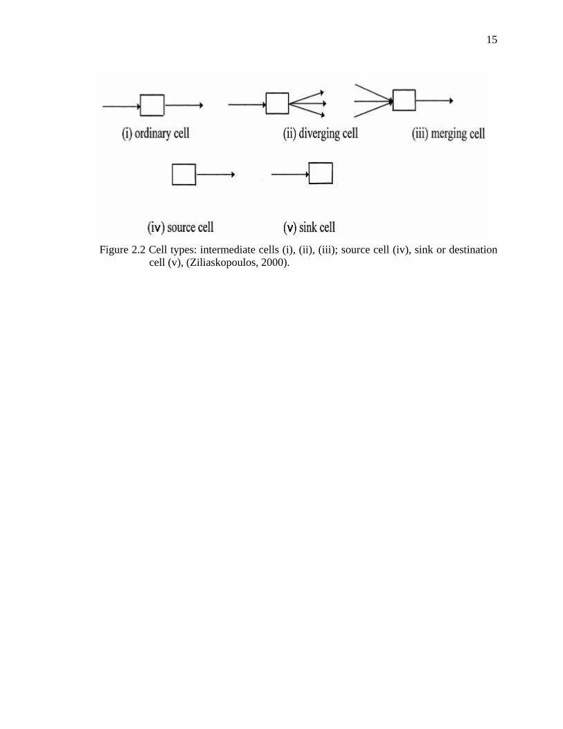
Figure 2.2 Cell types: intermediate cells (i), (ii), (iii); source cell (iv), sink or destination

cell (v), (Ziliaskopoulos, 2000). ...................................................................... 15

Figure 2.3 Fundamental traffic flow-density relationship (Lighthill and Whitham, 1955;

Richards, 1956). .............................................................................................. 16

Figure 2.4 Linear approximation of the fundamental flow-density relationship (Daganzo,

1994). .............................................................................................................. 17

Figure 2.5. Freeway contra-flow use configurations (Wolshon, 2005). ........................... 18

Figure 3.1 Methodological components. .......................................................................... 39

Figure 3.2 A bottleneck formed by the flow capacity of a highway ramp ....................... 40

Figure 4.1 CTM traffic flow relationship. ........................................................................ 48

Figure 5.1 Test network. ................................................................................................... 65

Figure 5.2 Cumulative curves of evacuees in the safety zone for different number of

reversed links. ................................................................................................. 66

Figure 5.3 Clearance time as a function of the number of reversed links. ....................... 67

Figure 5.4 Evacuation rate per minute for different numbers of reversed links. .............. 68

Figure 5.5 Improved network with 2 reversed links for 5000 evacuees uniformly

distributed to 20 sources and routed to 4 destinations (SID 1.2). ................... 69



vi

Figure Page














distributed to 20 sources and routed to 4 destinations (SID 1.9). .................. 77


distributed to 20 sources and routed to 4 destinations (SID 1.10). ................ 78

Figure 5.15 Computational time for 1% optimality gap. .................................................. 79

Figure 5.16 Network clearance time as a function of computational time for different

number of reversed links. ................................................................................ 80

Figure 5.17 Cumulative curves of evacuees in the safety zone for different population

sizes with 8 reversed links. ............................................................................. 81

Figure 5.18 Clearance time as a function of evacuee population with 8 reversed links. .. 82

Figure 5.19 Evacuation rate per minute for different evacuee population sizes with 8

reversed links. ................................................................................................. 83

Figure 5.20 Improved network with 8 reversed links for all population size scenarios

uniformly distributed to 20 sources and routed to 4 destinations (SID 2.1-

2.10). ............................................................................................................... 84

Figure 5.21 Cumulative curves of evacuees in the safety zone for different spatial

distributions of evacuation demand with 6 reversed links. ............................. 85

vii

Figure Page

Figure 5.22 Clearance time as a function of the spatial distribution of evacuation demand

for 6 reversed links.......................................................................................... 86

Figure 5.23 Evacuation rate per minute for different scenarios of spatial evacuation

distribution with 6 reversed links. ................................................................... 87


distributed to 20 sources and routed to 4 destinations (SID 3.1). .................. 88

Figure 5.25 Improved network with 6 reversed links for 5000 evacuees randomly

distributed to 20 sources and routed to 4 destinations (SID 3.2). The

highlighted cells indicated greater population centers. ................................... 89

Figure 5.26 Improved network with 6 reversed links for 5000 evacuees in a 1 source (cell

142, highlighted) and routed to 4 destinations (SID 3.3). ............................... 90


distributed to 2 sources (cells 142 and 134, highlighted) and routed to 4

destinations (SID 3.4). .................................................................................... 91


distributed to 20 sources and routed to 1 destination (cell 148, highlighted),

(SID 3.5). ........................................................................................................ 92


distributed to 20 sources and routed to 2 destinations (cells 147 and 150,

highlighted), (SID 3.5). ................................................................................... 93

viii

LIST OF TABLES

Table Page

Table 3.1 Summary of the parameters of the ENDP formulation. .................................... 37

Table 3.2 Summary of the variables of the ENDP formulation. ....................................... 38

Table 5.1 Legend of the test network. ............................................................................... 59

Table 5.2 Cell characteristics of the test network. ............................................................ 60

Table 5.3 Cell characteristics for lane addition design options. ....................................... 61

Table 5.4 Cell characteristics according to contra-flow options. ...................................... 62

Table 5.5 Characteristic parameters of the experiment scenarios. .................................... 63

Table 5.6. 5000 evacuees randomly distributed to source cells in the random distribution

scenario. ............................................................................................................................ 64

1

CHAPTER 1. INTRODUCTION

1.1 Background and motivation

Evacuation is called for when a natural or man-made extreme event (e.g.

hurricane, flooding, hazmat release, or dirty bomb) strikes a populated area exposing the

population to immediate or foreseeable life-threatening danger. After the identification

of the boundaries of the affected or threatened area, an associated evacuation zone is

defined. All civilians in the evacuation zone have to be relocated individually, or with the

guidance of a responsible agency (such as an emergency management agency) to a safer

location, the safety zone.

The evacuation process is an extremely complicated and difficult task where the

agency addresses the efficient utilization and coordination of roadway capacities, traffic

management equipment, public transportation vehicles, and various emergency response

resources. For disasters which have a sufficient lead time (i.e. a short-notice disaster

such as a hurricane or flooding), evacuation management agencies determine alternate

evacuation routes a priori based upon the expected spatial-temporal impacts of the

disaster. Citizens are then given advisories on which major roadways to use for

evacuation. In the event that an unexpected disaster occurs (i.e. a no-notice disaster),

such as a dam burst or a bio-chemical attack, evacuating a large population becomes

2

more challenging due to the short lead time and highly unpredictable pedestrian and

vehicular traffic flows. In this case, evacuees may crowd roadways and significantly

cripple the entire transportation system rendering it inoperable.

The recent events associated with Hurricane Katrina and its aftermath, as well as

Hurricane Rita, is illustrative of the need to better understand the intricacies and multiple

facets of evacuation so that large-scale response to potential massive disasters is

integrative, effective and efficient. The central challenging objective is routing people to

the safety zone as soon as possible. An efficient routing plan is valuable because

evacuations result in traffic volumes that exceed the available network capacity (Cova

and Johnson, 2002).

An evacuation plan entails identifying the set of routes which enable the fastest

evacuation out of the evacuation zone. Dynamic traffic assignment (Peeta and

Ziliaskopoulos, 2001), which explicitly incorporates the time-dependency of traffic

flows, can be used to determine a routing plan.

A key impediment to the performance of an evacuation plan is the capacity of the

traffic facilities (links) in the network. Kwon and Pitt (2004) highlight the significance of

capacity addition to urban networks for enhancing network performance under

evacuation. Traditionally, capacity is added to a traffic network through the construction

of new lanes as part of a long-term planning process. For short-term events requiring

evacuation, contra-flow operations are an attractive low budget capacity relocation

option. Contra-flow options have been widely suggested for evacuation purposes as “the

3

only way out” (Wolshon, 2005). It is a low budget network re-design strategy that best

fits the needs of the spatial restrictions of the dense urban metropolitan environment.

Traffic control at intersections under evacuation is a challenging issue as most

traffic delays during an evacuation occur at intersections (Southworth, 1991). Cova and

Johnson (2002) proposed a lane-based evacuation strategy for eliminating intersecting

flows and minimizing merging flows. They organized routing in terms of non-

intersecting lanes which can either merge or diverge.

In summary, evacuation operations can be significantly more efficient if strategic

network improvements enable the fastest routing of evacuee population to the safety

zone. The evacuation planning process, which seeks to determine where additional

capacity is necessary in the network to enhance performance under evacuation, can be

viewed as a combination of a dynamic traffic assignment problem and a network design

problem. Both these problems are known for their significant computational complexity,

especially in the context of large-scale problems. The proposed research focuses on the

mechanism to identify the best network design options for deployment, as well as on

reducing the computational complexity of the associated solution methods.

1.2 Study objectives

The study seeks to develop a methodology to address the strategic planning

problem of capacity addition at a network-level for evacuation planning. The proposed

methodology should enable decision-makers to select in a time-efficient manner an

4

effective set of network design options for evacuation-related operations. The specific

objectives are:

1. Development of a model to address the evacuation network design problem.

The mathematical formulation should identify, in a planning context, the best network

design options (contra-flow operations and lane addition) that optimize evacuation under

resource limitations.

2. Enhancement of the formulation to address the evacuation network design

problem in a computationally more efficient manner. The problem-specific structure of

the formulation will be analyzed to develop a modified formulation that enables the

application of faster algorithms.

3. Sensitivity analysis of the evacuation planning models to derive insights for the

decision-makers. This is done by analyzing the models for different levels of capacity

addition, population size, and spatial distribution.

1.3 Organization of the research

The remainder of the research is organized as follows. Chapter 2 provides an

overview of the relevant literature in evacuation planning, network design problems, the

cell transmission model and its transportation planning applications. Chapter 3 defines

the problem of network design for evacuation planning and formulates it. In Chapter 4, a

key property of the cell transmission model is identified, and the related propositions are

introduced. The problem is mathematically re-formulated, according to these

5

propositions, to have its computational time significantly decreased. The complexity of

the formulation is identified and the identified network structure is discussed. In Chapter

5 some implementations issues are highlighted, the test network is described, and

sensitivity analysis is performed. Key insights for transportation planners and emergency

management agencies are identified. Chapter 6 summarizes the research and its

contributions, and provides future research directions.

6

CHAPTER 2. LITERATURE REVIEW

This chapter provides a brief review of the methodological aspects relevant to the

problem addressed in this study. Section 2.1 discusses the literature and characteristics

related to evacuation planning. Section 2.2 describes the cell transition model, which is

used as the traffic flow simulator for the study. Section 2.3 discusses aspects related to

evacuation for network design. Section 2.4 discusses some algorithmic issues. Section 2.5

summarizes the issues and identifies the characteristics of the proposed approach.

2.1 Evacuation planning

Evacuation planning is typically associated with well-defined scenarios such as a

deliberate disaster in a nuclear power plant or the evacuation of a low lying coastal zone

under a hurricane threat. This necessitates the identification of a physical area around the

nuclear power plant or the coastal area, labeled the zone or footprint, from which people

must be evacuated. The zone or footprint for a potential evacuation scenario is called the

evacuation planning zone or evacuation zone (CA DOT, 2002). All affected civilians

have to be routed from the evacuation zone to the safety zone, as shown in Figure 2.1. In

the figure, the area enclosed within the red-colored square is the evacuation zone and the

7

area enclosed between the red-colored and green-colored squares represents the safety

zone identified for the specific scenario.

The total evacuation time includes four components: initial warning time,

individual’s evacuation preparation time, network clearance time, and evacuation

verification time. The focus of evacuation planning from a transportation perspective is

network clearance time, which represents the time needed for the evacuation volume to

clear the network (Sheffi et al., 1981). The objective of minimizing the total time that

evacuees are present in the evacuation zone is equivalent to requiring the minimization of

the average time that an evacuee spends in the evacuation zone (Jarvis et al., 1982). This

represents a system optimal dynamic traffic assignment problem (Peeta and

Ziliaskopoulos, 2001).

Campos et al. (1999) seek k-optimal independent paths for vehicle routing in

emergency evacuation planning. The proposed algorithm identifies paths such that a

greater number of vehicles can be sent in minimum time to the safety zone. However, the

paths are not time-dependent, and no planning is considered for capacity additions to the

network.

The evacuation routing problem is characterized significantly by time

dependencies in traffic flow and the related dynamic phenomena (queue formation and

dissipation, spillbacks, etc.). As discussed in Chapter 1, this entails the need for dynamic

traffic assignment models. In Section 2.2, the cell transmission model (CTM) will be

introduced as the backbone for capturing dynamic traffic flows.

8

2.2 The cell transmission model

The cell transmission model is a simple approach for modeling traffic flow

consistent with the hydrodynamic theory (Daganzo, 1994). As illustrated in Figure 2.2,

the modeling elements for a traffic network are the cell and the cell connector. The cell is

a homogeneous section of a road. Its length is equal to the distance traveled at light traffic

conditions in one time interval. If the free flow speed is 70 mph and the time interval is

10 seconds then the length of this cell is approximately 1026 feet. The cell connectors

link sequential cells and are responsible for advancing the flow to the next cell(s). The

CTM linearly approximates the fundamental flow-density relation (Figure 2.3) at the cell

level (Figure 2.4).

In the CTM, a road is divided into homogeneous cells, numbered consecutively

from the upstream end of the road. Moreover, because cells represent link flow, flow

variability inside the links can be captured, which is not easily possible if traffic is

propagated by using link exit functions (Ziliaskopoulos, 2000). The cell transmission

model is macroscopic and flow propagation obeys the aggregate characteristics of traffic

flow. Therefore, the location of vehicles within a cell is not known, and the

acceleration/deceleration of vehicles cannot be captured realistically.

Consider a long highway link with no entrances and exits which is modeled with

sequential ordinary cells. Under light traffic, all vehicles in a cell can be assumed to

advance to the next cell at each tick of the clock:

11

t ti ix x++ = (2.1)

9

where tix is the number of vehicles in cell i C∈ in time interval t T∈ . It is assumed that

this equation holds true for all traffic flows unless queuing occurs. Queuing is modeled

by introducing two parameters:

(i) tiQ , the maximum flow from cell 1i − to i during time interval t T∈ (when the

clock advances from t to 1t + ), which is the equivalent of flow capacity.

(ii) tiN , the maximum number of vehicles that can be present in cell i C∈ in time

interval t T∈ , which is the equivalent of maximum density.

The measurement unit of the two variables is “vehicles”, and not “vehicles/hour”

or “vehicles/mile”. The amount of empty space in cell i C∈ in time interval t T∈ is

t ti iN x− . Then, the number of vehicles t

iy that can flow into i C∈ in time interval t T∈

is given by:

{ }1min , ,t t t t ti i i i iy x Q N x−= − (2.2)

The CTM is based on a recursion where the cell occupancy at time 1t + equals its

occupancy in time interval t T∈ , plus the inflow and minus the outflow:

1 1t t t ti i i ix x y y+ += + − (2.3)

The cell transmission model was extended for network flow (Daganzo, 1995), and

the single destination system optimum dynamic traffic assignment formulation on the cell

transmission basis was introduced by Ziliaskopoulos (2000). Since then, the cell

transmission based network formulation has been used for transportation planning

schemes like traffic signal coordination (Lo, 2000), lane addition in user-optimum traffic

10

assignment (Ukkusuri et al., 2004), and contra-flow operations (Tuydes and

Ziliaskopoulos, 2005).

2.3 Network design

Capacity addition to a network under a budget constraint has been addressed

under the label of network design (Fulkerson, 1958). A “project cost” is associated with

each candidate capacity addition project, and the summation of the costs of all selected

projects must satisfy the total budget constraint. However, the formulation considers a

static network, which is unable to capture the traffic dynamics of essence to evacuation.

Consideration of link performance functions to recognize congestion effects leads to a

quadratic formulation. Queue spillbacks cannot be modeled even with this modification.

Further, the formulation can only address the lane addition option.

Viswanath and Peeta (2003) formulated the Multi-commodity Maximal Covering

Network Design Problem (MMCNDP) for identifying critical routes for earthquake

response and seismically retrofitting bridges. The underlying concept is the identification

of critical links, which are enhanced under a budget constraint so as to sustain seismic

action. The key contribution is the synchronous optimization for both travel times and

coverage in a single framework. The traffic assignment is static and link capacity is not

considered as a constraint, as the focus is on enabling emergency personnel to reach the

affected areas rather than on civilian evacuation.

Wolshon (2005) proposes various contra-flow options for evacuation. He

describes three options as shown in Figure 2.5: (1) one opposite lane, (2) one opposite

11

lane and the shoulder of the direction of interest, and (3) all of the opposing lanes without

any shoulders.

Kwon and Pitt (2004) analyze the significance of capacity additions to the urban

network. They compare different evacuation strategies with contra-flow using the

DYNASMART (Jayakrishnan et al., 1995) simulator to analyze various capacity

configurations. However, they limit capacity changes only to freeway facilities.

Tuydes and Ziliaskopoulos (2004) formulate the single destination network re-

design problem, accounting for contra-flow operations using the CTM. The concept of

coupled cells is introduced, where capacity is shared between cells involving flows in

opposite directions. The capacity is split according to a continuous variable, the lane

reversibility factor. This makes the formulation computationally efficient, since it retains

the linearity of the system optimal formulation. However, as discussed hereafter, the

approach ignores the reduction in capacity due to reversed-flow lanes.

Reversed-flow lanes under the contra-flow option results in a significant capacity

reduction for those lanes when routing flows in the opposite direction (Wolshon, 2005).

This is because flow interactions occur between the two opposing physically non-

separated flows. Also, drivers routed in the contra-flow lanes are unfamiliar with contra-

flow driving (signage faced opposite, no known exit-turns).

Existing models typically use linear variables to address evacuation. Contra-flow

options are lane-based discrete network design strategies. Since they involve option-

specific planning characteristics, it is difficult to represent them using linear variables

with adequate realism. That is, since lane-reversal is discrete in nature, the continuous

12

characteristic of linear variables cannot handle these discrete options. Further, linear

variables cannot realistically capture option-specific budget and trained personnel

constraints. For example, if one lane is reversed, it may require the same budget

investment for island removal or signage addition as when three lanes are reversed.

Another key realism issue for existing models is that they do not adequately model the

problem of crossing flows at intersections. In reality, crossing flows under evacuation can

lead to gridlock. This entails the need for explicit constraints (and practical deployment)

to handle intersecting flow by preempting flow in some directions (by modifying signal

plans or through law enforcement personnel present at intersections). By not doing so,

existing models overestimate network performance under evacuation.

2.4 Algorithmic aspects

Li et al. (2003) introduce a computationally efficient algorithm. A minimum-cost

flow sub-structure is recognized and the Dantzig-Wolfe decomposition method is used.

Dantzig-Wolfe decomposition relies on the fact that generating columns is

computationally more efficient than solving the original problem. However, the

minimum-cost flow structure is identified as a sub-structure only, while the constraint

responsible for the backward wave propagation (related to traffic flow modeling realism)

is not analyzed further as part of the network structure. Thereby, the backward wave

propagation is assumed to occur at free-flow speeds, which is not realistic. Also, source

cells do not have an exact network representation and the destination cells are connected

directly to a super-destination, precluding robust cell representation. The cell capacity

13

and cell connector capacity constraints are not discussed, though they are required for a

precise statement of the minimum-cost flow problem. Finally, the formulation for

multiple destinations ignores the first-in, first-out (FIFO) issue.

2.5 Discussion

The overview of the literature indicates that there is a strong need for a

computationally efficient approach to capture the dynamic traffic phenomena of the

evacuee routing. The cell transmission model allows a linear formulation for dynamic

traffic assignment. However, computational efficiency can be achieved only when

specific properties of the formulation are exploited. In this study, we propose a

computationally efficient approach for evaluation planning as illustrated in Chapters 3

and 4. The proposed formulation allows for multiple capacity addition strategies, flow

priorities at intersections, and shelter allocation studies.

14

Figure 2.1 Evacuation and safety zones.

15

Figure 2.2 Cell types: intermediate cells (i), (ii), (iii); source cell (iv), sink or destination

cell (v), (Ziliaskopoulos, 2000).

16

Figure 2.3 Fundamental traffic flow-density relationship (Lighthill and Whitham, 1955;

Richards, 1956).

17

Figure 2.4 Linear approximation of the fundamental flow-density relationship (Daganzo,

1994).

18

Figu

re 2

.5. F

reew

ay c

ontra

-flo

w u

se c

onfig

urat

ions

(Wol

shon

, 200

5).

19

CHAPTER 3. METHODOLOGY

Chapter 3 introduces the evacuation problem addressed in the research. Section

3.1 describes the problem generically. Section 3.2 provides a mathematical statement of

the problem as well as the notation for the formulation. Section 3.3 introduces the

formulation for the Evacuation Network Design Problem (ENDP). Section 3.4 discusses

relevant computational aspects. Section 3.5 analyzes the problem complexity and relevant

computational aspects. The chapter concludes with a summary in Section 3.6.

3.1 Problem description

The evacuation network design problem (ENDP) is formulated here. It seeks to

identify the links whose capacities ought to be augmented, through contra-flow

mechanism or new lane construction, so as to minimize the total time spent in the

network over all evacuees subject to budget constraints on costs and personnel. It further

assumes that cross-directional flows are not permitted under evacuation. Hence, the

broader goal is to identify critical links vis-à-vis evacuation under specific security

threats.

Figure 3.1 illustrates the methodological components of the ENDP. There are two

key components: (i) the routing of the evacuees to the network, and (ii) the determination

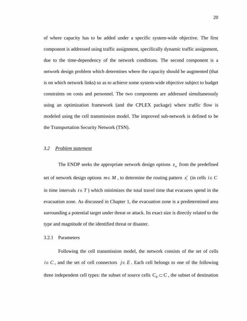
20

of where capacity has to be added under a specific system-wide objective. The first

component is addressed using traffic assignment, specifically dynamic traffic assignment,

due to the time-dependency of the network conditions. The second component is a

network design problem which determines where the capacity should be augmented (that

is on which network links) so as to achieve some system-wide objective subject to budget

constraints on costs and personnel. The two components are addressed simultaneously

using an optimization framework (and the CPLEX package) where traffic flow is

modeled using the cell transmission model. The improved sub-network is defined to be

the Transportation Security Network (TSN).

3.2 Problem statement

The ENDP seeks the appropriate network design options mz from the predefined

set of network design options m M∈ , to determine the routing pattern tix (in cells i C∈

in time intervals t T∈ ) which minimizes the total travel time that evacuees spend in the

evacuation zone. As discussed in Chapter 1, the evacuation zone is a predetermined area

surrounding a potential target under threat or attack. Its exact size is directly related to the

type and magnitude of the identified threat or disaster.

3.2.1 Parameters

Following the cell transmission model, the network consists of the set of cells

i C∈ , and the set of cell connectors j E∈ . Each cell belongs to one of the following

three independent cell types: the subset of source cells RC C⊂ , the subset of destination

21

cells SC C⊂ , and the subset of intermediate cells GC C⊂ . The set of the successor cells

of cell i C∈ is ( )iΓ and the set of the predecessor cells to cell i C∈ is 1( )i−Γ . The set of

discrete constant time intervals is t T∈ . The free flow speed for cell i C∈ is iv , the

traffic wave’s backward propagation speed for cell i C∈ is iw , and the ratio i iw v for

each cell i C∈ is iδ . The constant discretization time interval is τ and the demand

(inflow) at a source cell Ri C∈ in time interval t T∈ is tid . This parameter is responsible

for assigning the evacuee population to its starting time and location.

The network design options are denoted by m M∈ . The binary indicator mia

indicates whether the network design option m is associated with the cell i C∈ . Contra-

flow based network design is always associated with at least two opposite (coupled) cells.

For each of these cells and for the same design option, the binary indicator mia equals 1.

For contra-flow corridors, the associated network design options are associated with more

than one set of coupled cells. The initial maximum number of vehicles in cell i C∈ is

0iN . The maximum number of vehicles in cell ( )\ R Si C C C∈ ∪ , if network design

option m M∈ is implemented, is miN . Accordingly, the initial maximum number of

vehicles that can flow into or out of a cell in a time interval is 0iQ and the maximum

number of vehicles that can flow into or out of cell ( )\ R Si C C C∈ ∪ , if network design

option m M∈ is implemented, is miQ .

22

The maximum flow of cell connector j E∈ is jQ . It is pertinent to note that the

notion of an exact flow capacity jQ to a cell connector j E∈ is introduced for the first

time in the literature here. It is significant because it provides the ability to model the

bottleneck effect of right or left turns in an urban network. Right or left turns typically do

not have sufficient length to be modeled as individual cells. The CTM models the various

movements (right, straight or left) by limiting the inflows into these movements to be at

most the outflow from predecessor cells or the inflow to the successor cells. However,

this ignores the notion that turning movements have reduced capacities in reality. To

account for this issue, we propose capacity constraints for the cell connectors. This

represents an extension to the CTM.

The cost of implementing network design option m M∈ is mc , and the number

of trained personnel for the same option is mu . The cost mc of implementing a network

design option, or more specifically contra-flow operations, is the summation of all

budgetary costs like island redesign/removal for making the operations feasible, the cost

for training the personnel, and the cost of special equipment/facilities needed (cones,

signage, responder vehicles, personnel communication devices, and electronic variable

signage). The total budget is B and the total number of available personnel is U .

The set of intersections is l L∈ and the binary indicator jlβ indicates whether the

cell connector j E∈ is associated with intersection l L∈ . An intersection is defined to be

exactly two crossing flows (exactly two cell connectors) that cannot be realized in the

same time interval. For instance, in a four-way intersection, a crossing conflict is the left

23

turn of one direction and the opposite direction’s through movement. Only one of these

can be realized in the same time interval.

Table 3.1 summarizes the parameters of the ENDP formulation.

3.2.2 Variables

The formulation contains two categories of variables: the routing variables and

the network design variables. The routing variables are the number of vehicles tix in cell

i C∈ in time interval t T∈ and the number of vehicles tjy routed by cell connector j in

time interval t T∈ . The routing variables are non-negative real numbers. The network

design variable mz is a binary variable which indicates whether network design option

m M∈ is selected. The maximum number of vehicles in cell i C∈ for every time

interval t T∈ is iN . The maximum number of vehicles that can flow into or out of cell

i C∈ for every time interval t T∈ is iQ .

The binary variable jp indicates whether the flow of cell connector j E∈ is

restricted by an intersection constraint. When 1jp = , the flow represented by the cell

connector is assigned a green phase for all time intervals t T∈ . The variables iN and iQ

can be time-expanded to tiN and t

iQ . This allows addressing the question of when to add

capacity, in addition of where and how much to add. However, due to the combinatorial

nature of the network design part of the formulation, the complexity increases

exponentially without significant gains in terms of realism. So, even if the “best” capacity

addition strategy were time-dependent, the resources to deploy it may not be available.

24

Table 3.2 summarizes the variables used in the ENDP formulation.

3.3 Formulation of the ENDP

The objective of the formulation is to minimize the total time spent in the

network:

\

minS

ti

t T i C C

xτ∈ ∈

⋅∑ ∑

It minimizes the total vehicle-hours spent by all evacuees in the evacuation zone,

which consists of all the cells other than the destination cells. Since τ is a constant, it is

hereafter excluded from the mathematical formulation of the objective.

Another potential objective function in the evacuation context is the minimization

of the network clearance time. The network clearance time is the time elapsed between

when the evacuation order is given and when the last evacuee leaves the evacuation zone.

While the formulation objective function discussed above addresses the minimization of

the average travel time of the evacuees in the evacuation zone, it is mathematically

equivalent to the minimization of network clearance time (Jarvis et al., 1982).

The mixed-integer programming formulation for the ENDP is expressed as

follows:

minimize

\ S

ti

t T i C C

x∈ ∈∑ ∑

(3.3.1)

subject to:

25

( ) ( )1

1 1 1t t t ti i j j

j i j i

x x y y−

− − −

∈Γ ∈Γ

= − +∑ ∑

\ ,Ri C C t T∀ ∈ ∀ ∈ (3.3.2)

( )

1 1 1t t t ti i j i

j i

x x y d− − −

∈Γ

= − +∑

,Ri C t T∀ ∈ ∀ ∈ (3.3.3)

( )

t tj i

j iy x

∈Γ

≤∑

,i C t T∀ ∈ ∀ ∈ (3.3.4)

( )

tj i

j iy Q

∈Γ

≤∑

,i C t T∀ ∈ ∀ ∈ (3.3.5)

( )1

tj i

j i

y Q−∈Γ

≤∑

,i C t T∀ ∈ ∀ ∈ (3.3.6)

tj j jy p Q≤ ⋅ ,j E t T∀ ∈ ∀ ∈ (3.3.7)

( )( )

1

t tj i i i

j i

y N xδ−∈Γ

≤ −∑ ,i C t T∀ ∈ ∀ ∈ (3.3.8)

( ) 1mm i

m Mz a

∈

⋅ ≤∑

i C∀ ∈ (3.3.9)

( ) ( )01 m m mi i m i i m i

m M m MN a z N a z N

∈ ∈

⎛ ⎞= − ⋅ ⋅ + ⋅ ⋅⎜ ⎟⎝ ⎠

∑ ∑

( )\ ,R Si C C C t T∀ ∈ ∪ ∀ ∈ (3.3.10)

( ) ( )01 m m mi i m i i m i

m M m MQ a z Q a z Q

∈ ∈

⎛ ⎞= − ⋅ ⋅ + ⋅ ⋅⎜ ⎟⎝ ⎠

∑ ∑

( )\ ,R Si C C C t T∀ ∈ ∪ ∀ ∈ (3.3.11)

( )m mm M

z c B∈

⋅ ≤∑

(3.3.12)

( )m mm M

z u U∈

⋅ ≤∑

(3.3.13)

1jl jj E

pβ∈

⋅ ≤∑

l L∀ ∈ (3.3.14)

0tix ≥ ,i C t T∀ ∈ ∀ ∈ (3.3.15)

0tjy ≥ ,j E t T∀ ∈ ∀ ∈ (3.3.16)

{ }0,1mz ∈ m M∀ ∈ (3.3.17)

0iN ≥ i C∀ ∈ (3.3.18)

26

0iQ ≥ i C∀ ∈ (3.3.19)

{ }0,1jp ∈ j E∀ ∈ (3.3.20)

Equations (3.3.2) to (3.3.8) address the traffic flow modeling to route evacuees.

Equations (3.3.9) to (3.3.14) model the network design options and equations (3.3.15) to

(3.3.20) are the integrality and non-negativity constraints.

Equation (3.3.2) is the mass conservation constraint between cell and cell

connectors for all cells other than the source cells. The number of vehicles tix in cell

i C∈ in time interval t T∈ equals the number of vehicles 1tix − in the same cell in the

previous time interval plus the incoming flows from the incoming (predecessor) cell

connectors ( )1j i−∈Γ , minus the flows in the outgoing cell connectors ( )j i∈Γ .

Equation (3.3.3) addresses the conservation constraint at the source cells, and introduces

the demand tid at source cells Ri C∈ in time interval t T∈ . Equations (3.3.4) to (3.3.8)

linearly approximate the fundamental traffic flow-density relation (as discussed in

Section 2.3 and illustrated in Figure 2.4), taking into account holding of traffic at each

cell. Equation (3.3.4) models the free-flow region and states that the outflow on cell

connectors cannot exceed the number of vehicles in cell i C∈ in time interval t T∈ .

Equation (3.3.5) states that the total outflow from a cell through all the outgoing cell

connectors is less than the cell’s outflow capacity. Equation (3.3.6) states that the total

inflow into a cell through its incoming cell connectors is less than the cell’s inflow

capacity. By definition, since a cell is a homogeneous section of a road, its inflow and

27

outflow capacities are equal. Equation (3.3.7) is both the cell connector’s individual flow

capacity, as introduced and discussed previously, and the intersection flow restriction.

Equation (3.3.8) models the over-congested region of the fundamental flow equation,

where backward traffic wave effects are met. The flow is limited due to heavily

congested traffic conditions downstream. The speed of the backward propagating traffic

wave is i i iw vδ= ⋅ .

Equation (3.3.9) restricts the selection of network design options to be at most one

for each cell, since a single set of characteristic values (maximum flow iQ and maximum

number of vehicles iN ) must be assigned to every cell. If no network design option is

selected, a cell retains its initial parameters ( 0iQ , 0

iN ). This can be seen in equations

(3.3.10) and (3.3.11), where a cell’s maximum occupancy (3.3.10) and its maximum

inflow/outflow (3.3.11) take values that correspond either to the selected network design

option or their default values. Equations (3.3.12) and (3.3.13) are the budget and the

trained personnel constraints, respectively. The total budgetary cost and the total number

of required personnel cannot exceed the total available budget and the total available

trained personnel, respectively. Equation (3.3.14) allows at most one crossing flow to be

realized at an intersection, as defined previously.

3.4 Modeling issues

This section discusses pertinent modeling issues in relation to the formulation

discussed in the previous section.

28

3.4.1 Objective function

Tuydes and Ziliaskopoulos (2005) suggest a potential future extension that a

weighted system optimal objective be used instead of the traditional non-weighted system

optimal objective to capture behavioral effects. The weighted system optimal objective

seeks to capture the notion that the evacuees perceive that they are less threatened the

further they are from the target area. However, such an assumption can lead to skewed

performance as it focuses only on the distance from the target rather than whether there

are proportional benefits in terms of system performance clearance time and congestion

mitigation.

Further, in the context of network design, the weighted system optimal objective

is not adequate. The notion of routing evacuees even a single foot away without actually

evacuating them from the affected area, can lead to the use of the network design

resources for just providing more space for minor advancements than offering actual flow

capacity for evacuation. Hence, the traditional non-weighted system optimal objective

function is used for the model in this study.

A possible extension is to first solve for the network design options using the non-

weighted system optimal objective, and then, after introducing the optimal network

design options as parameters, solve using the weighted system optimal objective function

so as to derive a traffic pattern more consistent with the expected driver behavior.

29

3.4.2 Time to implement contra-flow operations

The time required to implement the contra-flow option affects the total

evacuation. It is the time between the issuance of the evacuation order and when the

contra-flow option is implemented in the traffic network. It is a function of the agency

preparedness, the location of the contra-flow implementation teams and the prevailing

traffic conditions. The accounting of the time of implementation can be performed

through two modifications to the problem formulation: (i) time expansion of the variables

ti iN N→ and t

i iQ Q→ , and b) identifying the time-dependent capacities for each

network design option m M∈ for the (same) cell i I∈ ; that is, it is possible that

( )1m tmti iN N +≠ .

The proposed modeling modifications significantly increase the complexity of the

problem. Hence, there is a need to analyze if the additional computational times are

justifiable, especially in an operational context. For some natural disasters such as

hurricanes, which have sufficient lead times, the evacuation order can be given after the

necessary contra-flow options have been implemented. In such instances, the time

expansion of the capacity variables is unnecessary. Since the research addresses a

planning context, the computational time for obtaining the contra-flow options is not

critical. However, the time required for implementing the contra-flow option in the field

may need to be factored, especially if the time required is not trivial.

30

3.4.3 Existence of shelters and capacity allocation

When planning for evacuation, there are three potential choices (or

“destinations”) to ensure the safety of the general population: (i) move the evacuee

outside the evacuation zone (as is done on this study), (ii) move the evacuee to a

designated shelter, and (iii) move the evacuee to a designated area at the origin itself

(designated “shelter room” in the building). A shelter can be easily modeled in the

current formulation as a destination cell with finite capacity sN . The formulation can

also model planning for construction of shelters, simply be reassigning a capacity msN to

the shelter s S∈ according to network design option m M∈ at a network design cost mc .

An interesting research question from a resource allocation standpoint is whether it is

better to build shelters or enhance the network through improvements (as is done in this

study) when constrained by a constant security budget.

3.4.4 Modeling contra-flow corridors

The contra-flow option can require performing the operation over several links or

a corridor, rather than at one link at a time (as is done in this study). It is a more realistic

option in some situations. The problem formulation can easily incorporate this network

design option. That is, a contra-flow corridor operation is a network design option mz that

assigns capacities mtiN and mt

iQ for two or more cells (that form a corridor)

simultaneously. The re-designed cells are indicated by setting the corresponding indicator

1mia = .

31

3.4.5 Traffic signal settings

There are three options related to traffic signals under an evacuation scenario: (i)

retain the existing signal plan, (ii) implement a modified “static” network-wide signal

plan for the duration of the evacuation, and (iii) implement a modified “dynamic”

network-wide signal plan. The first option simply retains the existing traffic signal

control pattern, which is not necessarily optimal from an evacuation standpoint. This is

because evacuation from a region is typically characterized by traffic directionality; that

is, there are heavy traffic flows in some directions. This motivates the need for modified

traffic signal plans for the evacuation duration. A modified “static” plan which is

assumed in our study, provides optimal priorities among intersecting directions, and

retains the same phase for each intersection for the evacuation period. Such a plan can

also be enforced using police officers at intersections, as is done currently at special

events such as football games. A “static” plan has key advantages: (i) it reduces the

likelihood of gridlock, and (ii) it is computationally efficient for implementation. A

modified “dynamic” signal plan seeks to relate signal phases to demand at the

intersection for each time interval in the evacuation period. While this might suggest the

best plan from a theoretical standpoint, it may not be particularly effective in practice.

This is because the density of traffic in roads can lead to non-compliance or partial

compliance of the signal settings by the evacuees. This behavior has been repeatedly

exhibited by drivers during special events, and can lead to inefficient blockage of key

intersections, resulting in gridlock conditions. Finally, the “dynamic” traffic control

32

approach is computationally intensive. Hence, the modified “static” plan is preferred, and

employed in our study.

3.4.6 FIFO property and bus routing

In a dynamic traffic assignment formulation it is important that the first in, first

out (FIFO) property be satisfied. To generate consistency with a single destination DTA,

under evacuation planning, all evacuees can be routed to a single destination, the safety

zone (Daganzo, 1994). This problem has been addressed in the literature as a single-

commodity network flow problem, where the FIFO property is inherently satisfied

(Ziliaskopoulos, 2000). However, it has the limitations discussed in Section 2.5.

The satisfaction of the FIFO property becomes a particularly challenging issue

when buses are routed to transfer low-mobility people out of the evacuation zone. A bus

carrying a significant number of evacuees can be assigned can be assigned a greater

weight, as it is a high occupancy vehicle. However, this can lead the optimization

software to deliberately violate FIFO in order to route the bus out of the evacuation zone

as quickly as possible.

3.4.7 Entry and exit flow capacities in evacuation zone

The flow capacities related to the entry and exit from the evacuation zone

significantly affect the network performance. Hence, the assumptions on these capacities

are a key modeling issue. An entry flow capacity is the outflow capacity of a source cell.

For example, it can be the flow capacity of a parking lot exit. An exit flow capacity of the

33

evacuation zone is the inflow capacity of the associated destination cell. For example, it

can be physically represented by the outflow from a boundary link in the evacuation zone

(Figure 3.2). If these flow capacities are assumed to be constants, then spatio-temporal

interactions arising from congestion on the adjacent cells and cell connectors are ignored.

Hence flow capacities of source and destination cells are assumed to be high enough so

that they are bounded only by the variable maximum flow capacity of the adjacent cells

and cell connectors.

Highway ramps are modeled as cell connectors which start or end at a highway

cell. The capacities of these cell connectors are those of the associated ramps. The

significance of this modeling approach is that it allows contra-flow operations to be

consistent with the actual ramp capacities. However, a drawback is that the travel time

spent in ramps is not captured. Ideally, highway ramps should be modeled as individual

cells in the CTM as they can require more than one time interval to negotiate the ramp

length at free-flow speeds. The trade-off is in terms of the additional computational and

modeling burden.

3.4.8 Comparison of contra-flow operations to lane addition

As discussed earlier, the network design options considered in this study are the

contra-flow options and lane addition. Contra-flow operations are cost-effective, flexible,

well-suited for dense urban environments, increasingly commonplace for mass

evacuations, and can be tailored to the evolving traffic/infrastructure conditions under the

unfolding disaster. By contrast, the lane addition option is expensive by several orders of

34

magnitude compared to the contra-flow option. Further it represents the addition of new

capacity to the network, and is hence purely a long-term planning strategy as the addition

of lanes requires a significant amount of time. Therefore, while the contra-flow option

can be addressed both in planning and operational contexts, the lane addition strategy is

meaningful only in the planning domain.

From an optimization standpoint, the asymmetric cost requirements of the two

options imply that the lane addition option is always dominated by the contra-flow option

under the same budget constraint for evacuation operations. Therefore, in Chapter 5, we

restrict our experiments to the contra-flow strategies.

3.5 Complexity

The ENDP is solved with the branch-and-cut algorithm in CPLEX. It is an exact

solution methodology for integer and mixed-integer programs. The computational cost in

is derived from two factors: (1) the number of tree nodes of the branch-and-cut algorithm,

and (2) the computational time at each tree node. To improve the computational effort,

specific network design options should be considered rather than searching the whole set

of network design options. As discussed in the next chapter, the use of the improved

formulation significantly reduces the computational time at each tree node.

The current formulation is a generalized mixed-integer formulation. The

constraints responsible for vehicle routing ((3.3.2) to (3.3.8)) are linear. The constraints

responsible for the network design options ((3.3.9) to (3.3.14)) involve binary variables,

leading a mixed integer formulation.

35

The computational experience with the ENDP formulation of Section 3.3 suggests

that it is highly intensive, even if the problem is fully linearized (that is, when the

network design options are not considered binary 0-1 variables). Even if only 10 network

design options are considered, the methodology requires a few days to obtain the solution

to within the pre-specified percentage optimality gap.

Chapter 4 discusses an improved ENDP formulation to enable greater

computational efficiency. It exploits key properties of the cell transmission model to

generate stricter bounds on the routing variables.

3.6 Summary

This chapter introduces the first formulation for the ENDP with combinatorial

network design options. It is a mixed-integer formulation which is composed of a set of

linear routing constraints ((3.3.2) to (3.3.8)), and a set of constraints responsible for the

network design options ((3.3.9) to (3.3.14)) that include binary variables. The advantage

of the combinatorial modeling approach for the network design options is that exact cell

parameters (in terms of flow and occupancy) are assigned depending on the specific

strategies: contra-flow operations, lane-addition or their combination. Planning for the

location and number of shelters can also be addressed. Moreover, capacity reduction (as

observed in the context of turning movements) was addressed by introducing of an

individual flow constraint for cell connectors representing turning movements.

Initial simulation experiments highlight the computationally intensive nature of

the formulation, and indicate the need for a more efficient formulation. The next chapter

36

discusses an improved formulation obtained by exploiting specific modeling

characteristics related to the CTM.

37

Table 3.1 Summary of the parameters of the ENDP formulation.

Parameter Description i C∈ The set of all cells.

RC C⊂ The subset of source cells (origin cells).

SC C⊂ The subset of destination cells.

GC C⊂ The subset of intermediate cells. j E∈ The set of cell connectors. ( )iΓ The set of the successor cells of cell i C∈ .

1( )i−Γ The set of the predecessor cells to cell i C∈ . t T∈ The set of discrete and constant time intervals. m M∈ The set of network design options.

mia The binary indicator showing if the network design option m is associated

with the cell i C∈ . 0iN The initial maximum number of vehicles in cell i C∈ . miN The maximum number of vehicles in cell ( )\ R Si C C C∈ ∪ , if network

design option m M∈ is implemented. 0iQ The initial maximum number of vehicles that can flow into or out of cell. miQ The maximum number of vehicles that can flow into or out of cell

( )\ R Si C C C∈ ∪ , if network design option m M∈ is implemented.

iv The free flow speed for cell i C∈ .

iw The traffic wave’s backward propagation speed for cell i C∈ .

iδ The ratio i iw v for each cell i C∈ . τ The constant discrete time interval’s length.

mc The cost of implementing design option m M∈ .

B The total available budget. mu The number of trained personnel needed for implementing capacity option

m M∈ . U The total number of available trained personnel.

tid The demand (inflow) at source cell Ri C∈ in time interval t T∈ .

jlβ The binary indicator showing if the flow in cell connector j E∈ can be restricted by intersection l L∈ .

38

Table 3.2 Summary of the variables of the ENDP formulation.

Variables Description tix The number of vehicles in cell i C∈ in time interval t T∈ tjy The number of vehicles moved by cell connector j E∈ in time interval

t T∈ .

mz The binary decision variable indicating if the network design option m M∈ is selected.

iN The maximum number of vehicles in cell i C∈ .

iQ The maximum number of vehicles that can flow into or out of cell i C∈ .

jp The binary variable indicating whether the flow in cell connector j E∈ is restricted by an intersection constraint.

39

Figure 3.1 Methodological components.

40

Figure 3.2 A bottleneck formed by the flow capacity of a highway ramp

41

CHAPTER 4. THE IMPROVED ENDP FORMULATION

This chapter discusses an improved formulation for the ENDP obtained by

exploiting specific characteristics related to the CTM. Section 4.1 illustrates some issues

with CTM. Section 4.2 identifies a mechanism to generate stricter bounds. Section 4.3

states propositions used to generate a computationally efficient formulation. Section 4.4

discusses the improved ENDP formulation. Section 4.5 describes its complexity. Section

4.6 provides some concluding comments for this chapter.

4.1 Properties of the cell transmission model

The linear approximation of the fundamental traffic flow equation used in the

CTM (Figure 2.4) has the following key characteristic: the light traffic flow region

extends up to the point P2 at which point the maximum flow is met, as shown in Figure

4.1. This implies that when the CTM is used as part a mathematical model, there is no

incentive for the optimizer to consider the region to the right of NFF. This modeling

approach is not necessarily the most realistic representation of the fundamental traffic

flow relationships. For example, the Highway Capacity Manual (2005) proposes that the

light traffic region end at a traffic density strictly less than the traffic density at the

42

maximum flow. This problem with the modeling approach of CTM, which raises issues

of realism, has not yet been discussed in the relevant literature.

4.2 Identification of stricter bounds

The issue discussed heretofore about the possible lack of realism in CTM’s

fundamental traffic flow relationship, is exploited to provide stricter bounds for the

formulation of the ENDP while assuring non-inferior solutions. Unlike in a pure routing

problem, the network design problem seeks to increase the maximum flow capacities.

Since these capacities are obtained at the bounds of the free-flow conditions, the

maximum occupancy iN of a cell i C∈ is reduced and set equal to the maximum number

of vehicles iQ that can propagate to the next cell(s). This is a key contribution of this

study, and leads to significant computational efficiencies.

4.3 Propositions

The introduction of the stricter bounds on the maximum occupancy iN of cell

i C∈ , hereafter equal (and equivalent) to iQ , justifies a set of propositions that simplify

the formulation, while generating non-inferior solutions (validated through the

computational experiment in Chapter 5). The propositions are:

(1) Backward propagating traffic waves are not meaningful at traffic densities

of light traffic conditions, and therefore constraint (3.3.8) is redundant.

43

(2) The maximum occupancy iN becomes equivalent to the maximum flow iQ ;

the iN variable and the associated equation (3.3.10) can be eliminated.

(3) The inequality (3.3.4) can be replaced by a strict equality for intermediate

cells; evacuees will be allowed to exit the source cells only if free-flow

conditions are guaranteed along the entire route from the origin to the

destination cell.

Although proposition (3) does not produce a realistic routing pattern for

evacuation, it still produces non-inferior solution sets for the ENDP. This is because there

is no incentive for the optimizer to push flow out of the source cells unless it can be led

without intermediate delays to the destination cells. This proposition can be regarded as a

relaxed analog of stage-based evacuation models.

The three propositions hold because it is assumed that at most one out of every

pair of crossing flows is allowed for the whole study period. If a traffic signal were to

allow different crossing flows for different time intervals, there may be an incentive to

increase the occupancy of at least one cell before the signal turns green so as to propagate

the maximum flow in the next few time intervals. However, in our study, we assume a

“static” traffic signal plan as discussed in Section 3.4.5. This limits the intersecting flow

at any intersection to be at most one such flow, for the evacuation period.

4.4 The improved formulation

The improved formulation, labeled iENDP, is as follows:

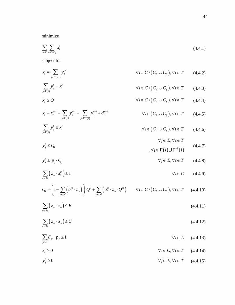
44

minimize

\ S

ti

t T i C C

x∈ ∈∑ ∑ (4.4.1)

subject to:

( )1

1t ti j

j i

x y−

−

∈Γ

= ∑ ( )\ ,R Si C C C t T∀ ∈ ∪ ∀ ∈ (4.4.2)

( )

t tj i

j iy x

∈Γ

=∑ ( )\ ,R Si C C C t T∀ ∈ ∪ ∀ ∈ (4.4.3)

ti ix Q≤ ( )\ ,R Si C C C t T∀ ∈ ∪ ∀ ∈ (4.4.4)

( ) ( )1

1 1 1 1t t t t ti i j j i

j i j i

x x y y d−

− − − −

∈Γ ∈Γ

= − + +∑ ∑ ( ) ,R Si C C t T∀ ∈ ∪ ∀ ∈ (4.4.5)

( )

t tj i

j iy x

∈Γ

≤∑ ( ) ,R Si C C t T∀ ∈ ∪ ∀ ∈ (4.4.6)

tj iy Q≤

,j E t T∀ ∈ ∀ ∈

( ) ( )1, j i i−∀ ∈Γ ΓU (4.4.7)

tj j jy p Q≤ ⋅ ,j E t T∀ ∈ ∀ ∈ (4.4.8)

( ) 1mm i

m Mz a

∈

⋅ ≤∑

i C∀ ∈ (4.4.9)

( ) ( )01 m m mi i m i i m i

m M m MQ a z Q a z Q

∈ ∈

⎛ ⎞= − ⋅ ⋅ + ⋅ ⋅⎜ ⎟⎝ ⎠

∑ ∑

( )\ ,R Si C C C t T∀ ∈ ∪ ∀ ∈ (4.4.10)

( )m mm M

z c B∈

⋅ ≤∑

(4.4.11)

( )m mm M

z u U∈

⋅ ≤∑

(4.4.12)

1jl jj E

pβ∈

⋅ ≤∑

l L∀ ∈ (4.4.13)

0tix ≥ ,i C t T∀ ∈ ∀ ∈ (4.4.14)

0tjy ≥ ,j E t T∀ ∈ ∀ ∈ (4.4.15)

45

{ }0,1mz ∈ m M∀ ∈ (4.4.16)

0iQ ≥ i C∀ ∈ (4.4.17)

{ }0,1jp ∈ j E∀ ∈ (4.4.18)

This formulation is a modification of the initial formulation discussed in Section

3.3. The constraints that differ from those in the original formulation are discussed

hereafter.

Equation (4.4.2) and (4.4.3) enforce free-flow traffic conditions in the

intermediate cells. The physical meaning is that since free-flow traffic conditions exist

(as discussed in Section 4.3), the number of vehicles propagated to the next cell(s) is

equal to the number of vehicles existing in the current cell in that time interval.

Equation (4.4.4) establishes stricter bounds on intermediate cell occupancies; it is

the upper bound of traffic density that allows free-flow speed conditions. There is no

need for equations (such as (3.3.8)) to track congested and the over-congested traffic flow

regions, since the problem is studied only in the free-flow region.

4.5 Complexity of the iENDP

Lemma : The iENDP is NP-hard.

Proof : It is proved by reduction. Consider the instance iENDPR of the

iENDP without the trained personnel constraint (4.4.12) and the intersection constraint

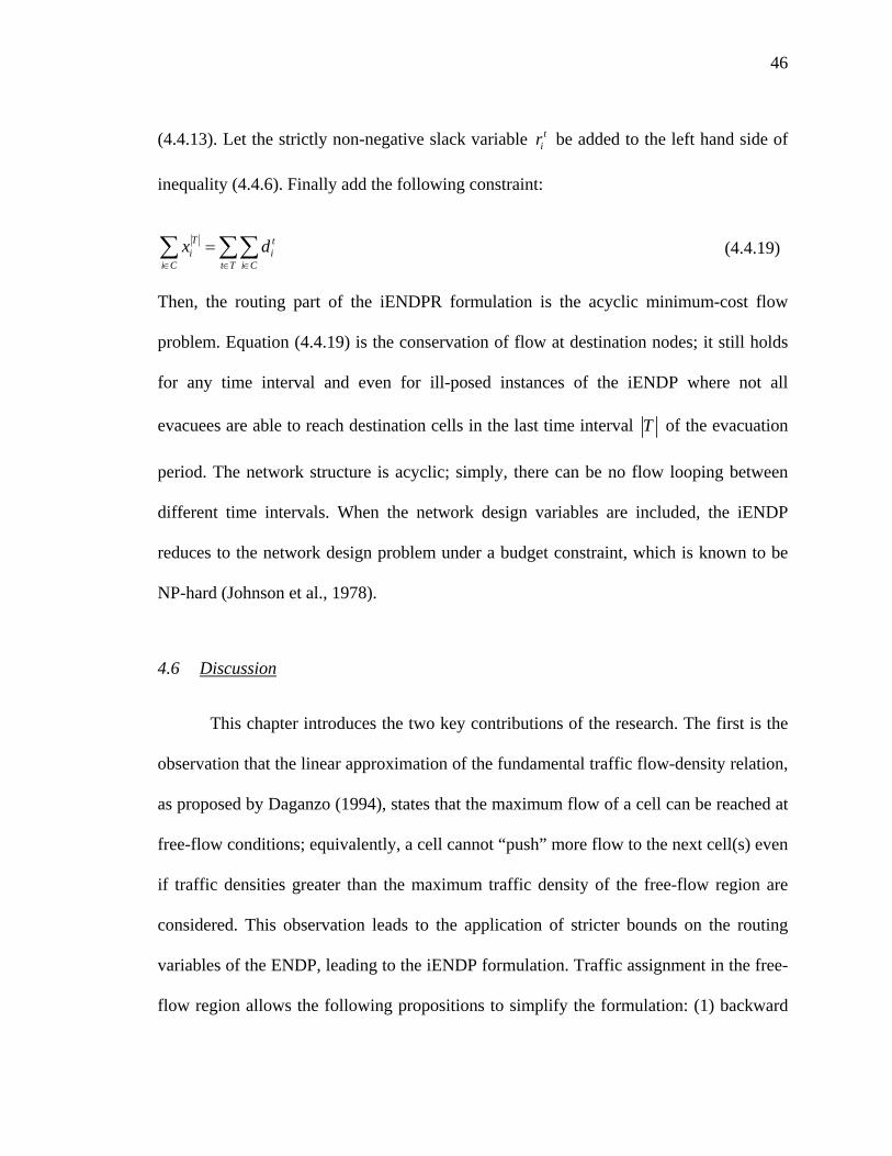
46

(4.4.13). Let the strictly non-negative slack variable tir be added to the left hand side of

inequality (4.4.6). Finally add the following constraint:

T ti i

i C t T i Cx d

∈ ∈ ∈

=∑ ∑∑ (4.4.19)

Then, the routing part of the iENDPR formulation is the acyclic minimum-cost flow

problem. Equation (4.4.19) is the conservation of flow at destination nodes; it still holds

for any time interval and even for ill-posed instances of the iENDP where not all

evacuees are able to reach destination cells in the last time interval T of the evacuation

period. The network structure is acyclic; simply, there can be no flow looping between

different time intervals. When the network design variables are included, the iENDP

reduces to the network design problem under a budget constraint, which is known to be

NP-hard (Johnson et al., 1978).

4.6 Discussion

This chapter introduces the two key contributions of the research. The first is the

observation that the linear approximation of the fundamental traffic flow-density relation,

as proposed by Daganzo (1994), states that the maximum flow of a cell can be reached at

free-flow conditions; equivalently, a cell cannot “push” more flow to the next cell(s) even

if traffic densities greater than the maximum traffic density of the free-flow region are

considered. This observation leads to the application of stricter bounds on the routing

variables of the ENDP, leading to the iENDP formulation. Traffic assignment in the free-

flow region allows the following propositions to simplify the formulation: (1) backward

47

propagating traffic waves can be ignored, (2) the maximum occupancy variable iN and

the equivalent definitional constraint (3.3.10) are redundant, and (3) evacuees are allowed

to exit the source cells only if free-flow conditions are guaranteed. The experiments in

the next chapter confirm that these propositions produce non-inferior solutions to the

ENDP.

The iENDP formulation is proven to be NP-Hard. This highlights the significance

of the second key contribution of the research. We identify that the cell transmission

model has an acyclic minimum cost flow structure for the routing constraints. This is

important because it enables the reduction of the computational complexity. Further, it

leads to the proposition of a generalized graph theoretic sub-structure for the CTM. The

generalized graph theoretic CTM has the potential for more efficient formulation of

several common problems in the transportation arena.

48

Figure 4.1 CTM traffic flow relationship.

49

CHAPTER 5. COMPUTATIONAL EXPERIMENTS

This chapter discusses computational experiments using a test network to derive

insights on the performance of the proposed evacuation model as well as on the

implications for practical deployment. Section 5.1 discusses some implementation issues.

Section 5.2 describes the test network and the experimental setup. Section 5.3 discusses

experiments and insights on evacuation strategies using several test scenarios. It also

discusses sensitivity analyses for key model parameters. The chapter concludes with a

summary of the experimental insights.

5.1 Implementation issues

This section discusses key issues that arise in the implementation of the

evacuation model for deriving insights through experiments.

5.1.1 Data on budget costs and trained personnel requirements

As discussed in Chapter 3, each network design option is associated with

budgetary costs and number of trained personnel requirements. For example, lane

addition is associated with an increased budgetary cost only, while contra-flow operations

are associated with a number of required trained personnel and a small budgetary cost

50

mostly related to island removal/reconstruction. However, two issues can potentially arise

in the model implementation context. First, data on budget and personnel needs for

contra-flow options require a dedicated study on the part of the responsible transportation

agency. Hence, these data are difficult to obtain currently, though this may not be an

issue in the future as security/disaster preparedness plans become more commonplace. To

circumvent this issue, the budget and trained personnel constraints in (3.3.12), (3.3.13),

(4.4.11), (4.4.12) are substituted by a more transparent constraint on the number of

contra-flow options allowed or equivalently the number of reversed links (RL). That is,

the number of reversed links (RL) allowed is used as a proxy for the budget and number

of trained personnel required for the corresponding contra-flow option.

5.1.2 Initial traffic conditions

The number of vehicles that need to be evacuated from the evacuation zone is

approximately equal to the sum of number of vehicles in parking lots in the evacuation

zone and the number of vehicles traveling on the links of the evacuation zone at the time

of the evacuation order. To account for the latter group of vehicles (vehicles in the

network links at the time of the evacuation order), all intermediate cells of the simulator

(ordinary, merging, diverging) are assigned an initial estimate of vehicles 0id , 0 0

i id N≤

at time t=0. The initial estimate is either based on historical data, or is obtained from the

sensor data on the day of the evacuation order.

However, there is a trade-off between realism and computational times. The

improved ENDP formulation assumes traffic assignment at free-flow conditions for

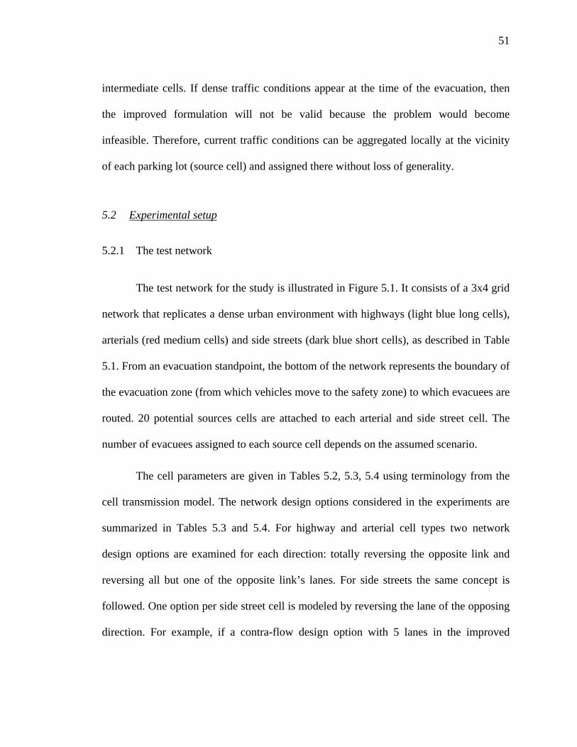
51

intermediate cells. If dense traffic conditions appear at the time of the evacuation, then

the improved formulation will not be valid because the problem would become

infeasible. Therefore, current traffic conditions can be aggregated locally at the vicinity

of each parking lot (source cell) and assigned there without loss of generality.

5.2 Experimental setup

5.2.1 The test network

The test network for the study is illustrated in Figure 5.1. It consists of a 3x4 grid

network that replicates a dense urban environment with highways (light blue long cells),

arterials (red medium cells) and side streets (dark blue short cells), as described in Table

5.1. From an evacuation standpoint, the bottom of the network represents the boundary of

the evacuation zone (from which vehicles move to the safety zone) to which evacuees are

routed. 20 potential sources cells are attached to each arterial and side street cell. The

number of evacuees assigned to each source cell depends on the assumed scenario.

The cell parameters are given in Tables 5.2, 5.3, 5.4 using terminology from the

cell transmission model. The network design options considered in the experiments are

summarized in Tables 5.3 and 5.4. For highway and arterial cell types two network

design options are examined for each direction: totally reversing the opposite link and

reversing all but one of the opposite link’s lanes. For side streets the same concept is

followed. One option per side street cell is modeled by reversing the lane of the opposing

direction. For example, if a contra-flow design option with 5 lanes in the improved

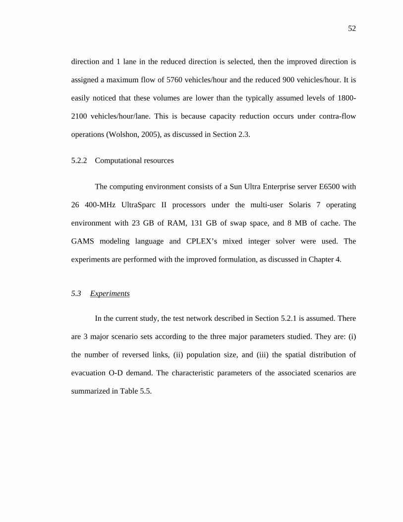
52

direction and 1 lane in the reduced direction is selected, then the improved direction is

assigned a maximum flow of 5760 vehicles/hour and the reduced 900 vehicles/hour. It is

easily noticed that these volumes are lower than the typically assumed levels of 1800-

2100 vehicles/hour/lane. This is because capacity reduction occurs under contra-flow

operations (Wolshon, 2005), as discussed in Section 2.3.

5.2.2 Computational resources

The computing environment consists of a Sun Ultra Enterprise server E6500 with

26 400-MHz UltraSparc II processors under the multi-user Solaris 7 operating

environment with 23 GB of RAM, 131 GB of swap space, and 8 MB of cache. The

GAMS modeling language and CPLEX’s mixed integer solver were used. The

experiments are performed with the improved formulation, as discussed in Chapter 4.

5.3 Experiments

In the current study, the test network described in Section 5.2.1 is assumed. There

are 3 major scenario sets according to the three major parameters studied. They are: (i)

the number of reversed links, (ii) population size, and (iii) the spatial distribution of

evacuation O-D demand. The characteristic parameters of the associated scenarios are

summarized in Table 5.5.

53

5.3.1 Design of experiments

The first scenario set examines the effect of different levels of resource allocation

for the network design options. Only contra-flow operations are assumed, and as

discussed in Section 3.4.8, the resource allocation is quantified by using the number of

reversed links as a proxy. Hence, reversed links ranging from 0 to 20 are examined for a

uniform distribution of 5000 evacuees to 20 sources. It is expected that these experiments

will provide insights on the “ideal” levels of resource allocation for the decision-makers

(or planners). The experiments also analyze the computational time efficiencies.

The second scenario set examines the effect of the population size on the

evacuation performance for a constant number of reversed links, acquired after the

analysis of the first scenario set. It is the number of reversed links at which most of the

improvement in network performance is achieved. For this number of reversed links (8),

population sizes of 500 to 5000 evacuees are assigned to 20 sources.

The third scenario set examines the effect of the spatial distribution of the

transportation demand for evacuation. 5000 evacuees are assigned to 1 source, 2 sources

uniformly, and 20 sources uniformly and randomly, and routed to 1 destination, 2

destinations, and 4 destinations. It seeks insights on the topological properties of the

selected reversed links. Table 5.6 illustrates the distribution of demand under the random

demand distribution scenario.

The three scenarios are evaluated using cumulative curves of evacuees exiting the

evacuation zone (as in Figures 5.2, 5.17 and 5.21), the network clearance time (as in

54

Figures 5.3, 5.18 and 5.22), the evacuation rate (as in Figures 5.4, 5.19 and 5.23), and the

graphical view of the test network with the selected reversed links (as in Figures 5.5-5.14,

5.20, and 5.24-5.29). Also, the computational time as a function of the number of

reversed links and clearance time is analyzed in Figures 5.15 and 5.16.

5.3.2 Effect of resource allocation on evacuation performance for uniformly distributed

population

The cumulative curves of evacuees exiting the evacuation zone for various

numbers of reversed links are illustrated in Figure 5.2. The network clearance time,

defined in Section 2.1, is used to analyze the network performance under various

resource (number of reversed links) constraints. The initial network of 0 reversed links

entails a clearance time of 22 minutes. The corresponding value for 20 reversed links is

14 minutes, representing a 36% reduction in network clearance time. This implies that

using the contra-flow option in dense urban environments can lead to significant

performance enhancements under security-related mass evacuation scenarios. An

important practical insight is that most of the potential benefits through contra-flow

operations are realized when 8 reversed links are allocated, which results in a network

clearance time of 15.9 minutes (Figure 5.3). This illustrates that there is an optimal level

of resource allocation beyond which additional benefits are insignificant. This implies

that decision-makers (traffic operators) can determine effective contra-flow strategies by

identifying the best level of resource allocation from a cost-benefit perspective.

55

Figure 5.2 further illustrates the sigmoid nature of the cumulative network

clearance time curve. The evacuation rate (rate of arrivals to the destination cells),

represented by the tangent of the cumulative curve, initially increases. It reaches a

maximum rate, and then keeps decreasing. The evacuation rate is illustrated in Figure 5.4.

The various characteristics of the results can be explained by tracking the time-dependent

nature of traffic congestion. Initially, the clearance rate increases as demand is being

serviced below capacity, that is, the network is not congested to capacity. As further

demand is serviced, the network links reach their capacities and that is represented by the

region of the maximum evacuation rate. As time progresses, demand decreases leading to

reduced evacuation rates until all traffic is cleared from the evacuation zone.

The various network design options are illustrated graphically in Figures 5.5-5.14.

The selected reversed links for contra-flow operations are indicated with thick lines

according to the color coding discussed in Table 5.1. There is a clear topological trend in

terms of the formation of contra-flow corridors with increased resources. The reversed

links start forming close to the destination cells of the test network and extend inwards to

form corridors as the number of reversed links increase. This is because of the

directionality of the evacuation flows which makes the capacity closer to the destinations

critical in terms of enabling efficient evacuation rates. After the 8 reversed links case, a

general tree structure is exhibited. It is important to note that most of the improvement of

the network clearance time is achieved at the level of 8 reversed links.

Figure 5.15 plots the relationship between the number of reversed links and the

computational time. It indicates that the computational time increases exponentially with

56

the number of allocated reversed links. Figure 5.16 indicates a marginal improvement in

clearance time as computational times increase beyond the 10-15 minutes range. Hence,

the insights from the computational times also suggest that beyond some resource

allocation levels, the benefits are marginal.

5.3.3 Effect of uniformly distributed population size on evacuation performance


population sizes (under uniform spatial distribution) are illustrated in Figure 5.17. The

initial population of 500 evacuees entails a clearance time of 2.5 minutes. The

corresponding value for 5000 evacuees is 15 minutes, representing a 600% increase in

network clearance time. Figure 5.18 suggests a linear relationship between the evacuee

population size and the network clearance time (under the uniform distribution). The

linearity is explained by the constant evacuation rate for a long time period. This

represents a useful insight for the decision-maker. Figure 5.19 illustrates the time-

dependent evacuation rates.

It is useful to note that for small evacuee population sizes, the evacuation rate

does not reach the network capacity. However, for large population sizes, the maximum

capacity of the network is reached and retained for a long time period, substantially

constraining the evacuation performance. It suggests long-term lane addition as a solution

to address evacuation needs of large populations. An interesting question is whether the

strategies “scale” for large populations, as population in a region increases over time.

57

The network design options under the various evacuee population sizes are

illustrated in Figure 5.20. The selected reversed links for contra-flow operations are

indicated with thick lines according to the color coding discussed in Table 5.1. Although

some trivial variations exists among the different population sizes, the trend is the one

represented in Figure 5.20, and is identical to the solution for the 8 reversed links with

5000 evacuees uniformly distributed to 20 sources (Figure 5.8).

5.3.4 Effect of spatial distribution of evacuation demand on network performance


scenarios of spatial distribution under the 6 reversed links case are illustrated in Figure

5.21. The examined scenarios are combinations of single or multiple sources and/or

destinations, as illustrated in Table 5.5. These scenarios are discrete and cannot be

physically examined in a continuous manner. The results suggest that the patterns with

multiple sources, multiple destinations, and uniform spatial distributions lead to better

clearance times (Figure 5.22). This trend is reasonable as multiple sources and

destinations avoid local congestion hotspots that can occur due to concentration of

demand at few locations. Further, as expected, the uniform distribution scenario performs

better than the random distribution scenario. Figure 5.23 illustrates that the larger the

amount of time when the bottleneck (severe congestion) exists, the more linear the

evacuation curve is.

The various network design options are illustrated in Figures 5.24-5.29. The

selected reversed links for contra-flow operations are indicated with thick lines according

58

to the color coding discussed in Table 5.1. They indicate that capacity is added where

bottlenecks exist. This is easily observed especially in the scenarios with 1 or 2 sources or

sinks. It is important to note that for the scenarios with 1 and 2 sources to many

destinations, there exist links that do not reduce bottlenecks, like 52 and 54 for both

scenarios (Figures 5.26 and 5.27). That is, the bottleneck has been optimally improved,

and the reversal of links 52 and 54 does not provide additional benefits (it simply satisfies

the 6 reversed links requirement).

5.4 Summary

The numerical and topological properties, as observed through the different

scenarios are of special interest to planners. In the first set of scenarios, it was identified

that solving for a specific size of resources is adequate for a “good” solution. In the

second set of scenarios, a linear relation between clearance time and population size was

illustrated, which provides insights on the capabilities for efficiently solving evacuation

problems with large populations through reduced computational times. The third set of

scenarios indicated that multiple origins and destinations, and greater uniformity in the

spatial distribution of demand lead to better network performance under evacuation.

59

Table 5.1 Legend of the test network.

60

Table 5.2 Cell characteristics of the test network.

Cell Type Highway Arterial Side Street Source DestinationCell IDs 1-22 23-78 79-126 127-146 147-150 Free flow speed (miles/h) 70 35 20 - - Time interval (sec) 10 10 10 10 10 Cell length (feet) 1000 500 250 - - Number of lanes 3 2 1 3 3 Maximum flow per lane (veh/hour/lane) 2160 1800 1800 2160 2160

Maximum cell flow 18 10 5 infinite infinite Reduced maximum cell flow (veh/time step) (due to the evacuation operations)

12 7 3 12 12

Number of vehicles per cell (veh/cell) 108 36 9 infinite infinite

61

Table 5.3 Cell characteristics for lane addition design options.

Cell type Flow capacity increase for the addition of one lane (veh/hour)

Flow capacity increase for the addition of one lane (veh/time step of 10 sec)

Lane addition cost per mile per lane (in million $)

Lane addition cost per cell (in million $)

Highway 1440 4 2 0.4 Arterial 1260 3.5 2 0.2

Side Street 1080 3 2 0.1

62

Table 5.4 Cell characteristics according to contra-flow options.

Final number of lanes per direction

Maximum cell flow Qi (veh/h)

Maximum cell flow Qi (veh / time step

of 10 sec) Direction Improved Reduced Improved Reduced Improved Reduced

Highway cell (3 lanes per direction)

5 1 5760 900 16 2.5

6 0 7200 0 20 0

Arterial cell (2 lanes per direction)

3 1 3240 720 9 2

4 0 4320 0 12 0

Side street cell (1 lane per direction)

2 0 1800 0 5 0

63

Table 5.5 Characteristic parameters of the experiment scenarios.

Scenario ID

(SID)

Description Population size

Spatial distribution

of the population

Number of

sources

Number of destinations

Number of

reversed links

1.1

Number of reversed

links

5000 Uniform 20 4 0 1.2 5000 Uniform 20 4 2 1.3 5000 Uniform 20 4 4 1.4 5000 Uniform 20 4 6 1.5 5000 Uniform 20 4 8 1.6 5000 Uniform 20 4 10 1.7 5000 Uniform 20 4 12 1.8 5000 Uniform 20 4 14 1.9 5000 Uniform 20 4 18 1.10 5000 Uniform 20 4 20 2.1

Population size

500 Uniform 20 4 8 2.2 1000 Uniform 20 4 8 2.3 1500 Uniform 20 4 8 2.4 2000 Uniform 20 4 8 2.5 2500 Uniform 20 4 8 2.6 3000 Uniform 20 4 8 2.7 3500 Uniform 20 4 8 2.8 4000 Uniform 20 4 8 2.9 4500 Uniform 20 4 8 2.10 5000 Uniform 20 4 8 3.1

Spatial distribution

of evacuation

demand

5000 Uniform 20 4 6 3.2 5000 Random 20 4 6 3.3 5000 Uniform 1 4 6 3.4 5000 Uniform 2 4 6 3.5 5000 Uniform 20 1 6 3.6 5000 Uniform 20 2 6

64

Table 5.6. 5000 evacuees randomly distributed to source cells in the random distribution scenario.

Source ID Population127 235 128 48 129 27 130 73 131 167 132 390 133 214 134 268 135 1042 136 203 137 429 138 81 139 234 140 398 141 111 142 67 143 343 144 97 145 436 146 137

65

Figure 5.1 Test network.

66

0

500

1000

1500

2000

2500

3000

3500

4000

4500

5000

0 1 2 3 4 5 6 7 8 9 10 11 12 13 14 15 16 17 18 19 20 21 22 23

Time elapsed from the beginning of the evacuation order (min)

Cum

ulat

ive

num

ber o

f eva

cuee

s in

safe

ty z

one

0 reversed links2 reversed links4 reversed links6 reversed links8 reversed links10 reversed links12 reversed links14 reversed links16 reversed links18 reversed links20 reversed links

Figure 5.2 Cumulative curves of evacuees in the safety zone for different number of reversed links.

67

18.8

16.5

15.915.6

15.215.0

14.714.4

14.1

17.5

22.1

12

14

16

18

20

22

0 2 4 6 8 10 12 14 16 18 20

Number of reversed links

Cle

aran

ce ti

me

(min

)

Figure 5.3 Clearance time as a function of the number of reversed links.

68

0

50

100

150

200

250

300

350

400

450

500

0 1 2 3 4 5 6 7 8 9 10 11 12 13 14 15 16 17 18 19 20 21 22 23


Evac

uatio

n ra

te p

er m

inut

e (e

vacu

ees/

min

.)0 reversed links2 reversed links4 reversed links6 reversed links8 reversed links10 reversed links12 reversed links14 reversed links16 reversed links18 reversed links20 reversed links

Figure 5.4 Evacuation rate per minute for different numbers of reversed links.

69

Figure 5.5 Improved network with 2 reversed links for 5000 evacuees uniformly distributed to 20 sources and routed to 4 destinations (SID 1.2).

70


distributed to 20 sources and routed to 4 destinations (SID 1.3).

71



72



73



74



75



76



77



78



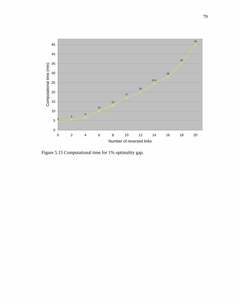
79

13

17

20

24.5

28

35

45

45

6

10

0

5

10

15

20

25

30

35

40

45

0 2 4 6 8 10 12 14 16 18 20

Number of reversed links

Com

puta

tiona

l tim

e (m

in)

Figure 5.15 Computational time for 1% optimality gap.

80

22.1

18.8

17.5

16.5

15.9

15.215.0

14.714.4

14.1

15.6

12

14

16

18

20

22

0 5 10 15 20 25 30 35 40 45

Computational time (min)

Net

wor

k cl

eara

nce

time

(min

)

Figure 5.16 Network clearance time as a function of computational time for different

number of reversed links.

81

0

500

1000

1500

2000

2500

3000

3500

4000

4500

5000

0 1 2 3 4 5 6 7 8 9 10 11 12 13 14 15 16 17 18 19 20 21 22 23


Cum

ulat

ive

num

ber o

f eva

cuee

s in

safe

ty z

one

500 Evacuees1000 Evacuees1500 Evacuees2000 Evacuees2500 Evacuees3000 Evacuees3500 Evacuees4000 Evacuees4500 Evacuees5000 Evacuees

Figure 5.17 Cumulative curves of evacuees in the safety zone for different population

sizes with 8 reversed links.

82

0

2

4

6

8

10

12

14

16

0 500 1000 1500 2000 2500 3000 3500 4000 4500 5000

Evacuee population

Cle

aran

ce ti

me

(min

)

Figure 5.18 Clearance time as a function of evacuee population with 8 reversed links.

83

0

50

100

150

200

250

300

350

400

450

500

0 1 2 3 4 5 6 7 8 9 10 11 12 13 14 15 16 17 18 19 20 21 22 23


Evac

uatio

n ra

te p

er m

inut

e (e

vacu

ees/

min

.) 500 Evacuees1000 Evacuees1500 Evacuees2000 Evacuees2500 Evacuees3000 Evacuees3500 Evacuees4000 Evacuees4500 Evacuees5000 Evacuees

Figure 5.19 Evacuation rate per minute for different evacuee population sizes with 8

reversed links.

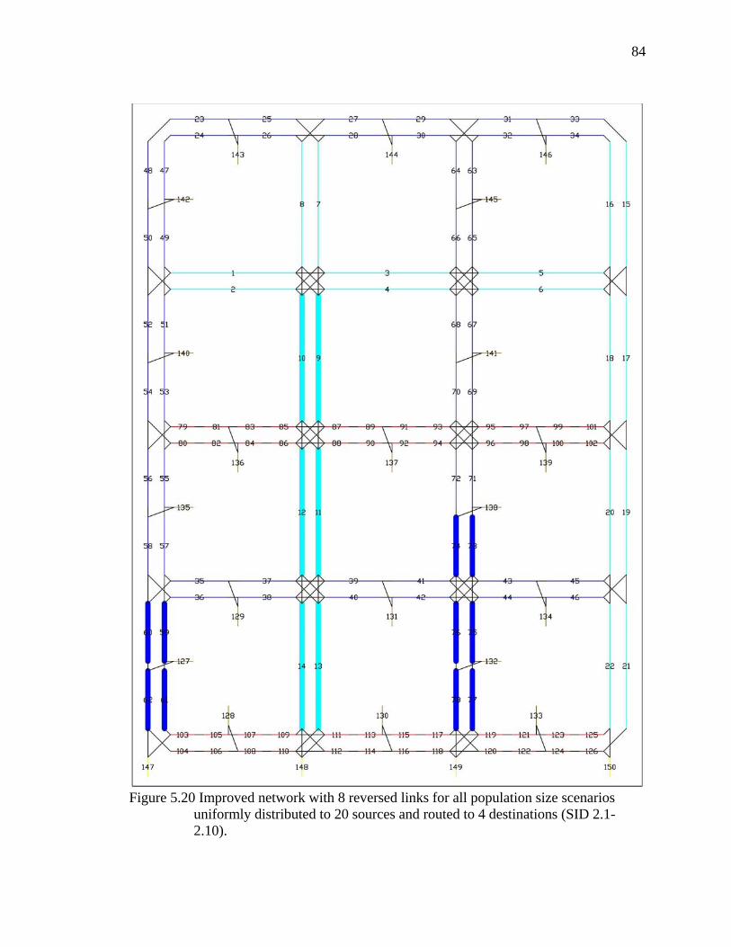
84

Figure 5.20 Improved network with 8 reversed links for all population size scenarios

uniformly distributed to 20 sources and routed to 4 destinations (SID 2.1-2.10).

85

0

500

1000

1500

2000

2500

3000

3500

4000

4500

5000

0 2 4 6 8 10 12 14 16 18 20 22 24 26 28 30 32 34 36 38 40 42 44


Cum

ulat

ive

num

ber o

f eva

cuee

s in

safe

ty z

one

Multiple sources - multipledestinations / uniformMultiple sources - multipledestinations / random1 source - multiple destinations

2 sources - multiple destinations

Multiple sources - 1 destination

Multiple sources - 2 destinations

Figure 5.21 Cumulative curves of evacuees in the safety zone for different spatial

distributions of evacuation demand with 6 reversed links.

86

42.7

31.9

29.2

25.5

18.516.2

0

5

10

15

20

25

30

35

40

45

1 source -multiple

destinations

Multiplesources - 1destination

Multiplesources - 2destinations

2 sources -multiple

destinations

Multiplesources -multiple

destinations /random

Multiplesources -multiple

destinations /uniform

Scenario

Cle

aran

ce ti

me

(min

)

Figure 5.22 Clearance time as a function of the spatial distribution of evacuation demand

for 6 reversed links.

87

0

50

100

150

200

250

300

350

400

450

500

0 2 4 6 8 10 12 14 16 18 20 22 24 26 28 30 32 34 36 38 40 42 44


Evac

uatio

n ra

te p

er m

inut

e (e

vacu

ees/

min

.)Multiple sources - multiple destinations /uniformMultiple sources - multiple destinations /random1 source - multiple destinations

2 sources - multiple destinations

Multiple sources - 1 destination

Multiple sources - 2 destinations

Figure 5.23 Evacuation rate per minute for different scenarios of spatial evacuation distribution with 6 reversed links.

88



89

Figure 5.25 Improved network with 6 reversed links for 5000 evacuees randomly

distributed to 20 sources and routed to 4 destinations (SID 3.2). The highlighted cells indicated greater population centers.

90

Figure 5.26 Improved network with 6 reversed links for 5000 evacuees in a 1 source (cell

142, highlighted) and routed to 4 destinations (SID 3.3).

91


distributed to 2 sources (cells 142 and 134, highlighted) and routed to 4 destinations (SID 3.4).

92


distributed to 20 sources and routed to 1 destination (cell 148, highlighted), (SID 3.5).

93


distributed to 20 sources and routed to 2 destinations (cells 147 and 150, highlighted), (SID 3.5).

94

CHAPTER 6. CONCLUSIONS

This chapter summarizes the research, highlights its contributions, and proposes

directions for future research.

6.1 Summary

In this study, capacity addition for an evacuation network design problem (ENDP)

was formulated as a mixed-integer program. The ENDP seeks to minimize the average

time that evacuees spend in the evacuation zone, by selecting the appropriate capacity

addition strategy among three potential options: (i) contra-flow operation, (ii) lane

addition, and (iii) combination of (i) and (ii). However, option (i) is a dominant option

and is hence analyzed through several computational experiments.

The formulation of the ENDP was improved to the iENDP by identifying a

special property of the cell transmission model; the maximum flow of a cell is reached at

the maximum density at which free-flow speed is achieved. This observation resulted in

the transformation of the linear routing constraints to an exact acyclic minimum cost flow

structure. The problem was found to be NP-hard, due to the integral network design

constraints.

95

Potential applications of the models developed in this study include contra-flow

operations for evacuation under a terrorist or hurricane threat, network re-design planning

for regular traffic situations including fixed one-way link design options, and peak hour

reversible lane operations. Transportation planning for installing variable contra-flow

signage and for contra-flow corridor operations can also be handled accurately through

the proposed approach.

6.2 Contributions of the research

This study defines the Evacuation Network Design Problem (ENDP) and

formulates it. From a practical standpoint, the overall contribution of this study is its

ability to address planning problems faced by emergency response agencies vis-à-vis

disaster management. The specific problem addressed here relates to effective evacuation

demand management. Under a resource constraint, there is a need to determine an

effective selection of links to be reversed so as to optimize network performance under

evacuation.

Most studies in the literature have adopted modeling approaches without

considering resources limitations, bottlenecks developed from ramp capacity, crossing

flows constraints, exact capacity addition options, corridor contra-flow operations, and

computationally efficient solution methodologies. This study addresses these critical gaps

by developing a single computationally efficient formulation. It does this by extending

the cell transmission model and exploiting several of its properties, further enhancing its

modeling capabilities and computational efficiency.

96

From the problem and methodological viewpoints, the contributions of the

research are:

1. Introduction of cell connector capacity constraint (Section 3.2.1). Its significance is

that it enables the modeling of the left/right turn capacity more realistically.

2. Exact combinatorial modeling of network design options (Section 3.2.2). The

capacity addition options (lane addition and contra-flow operations) are formulated

using the more generic concept of a “network design option”. This approach also

allows the modeling of shelter design options (Section 3.4.3), where a shelter is a

destination in the safety zone with a variable occupancy. It also enables the

modeling of contra-flow corridors (Section 3.4.4). Furthermore, the lane addition

option can equivalently model the effect of “releasing” a lane with parking

restriction policies on critical links.

3. Traffic signal control strategies (Section 3.4.5). To account for the constraining

effect of intersecting flows, three traffic signal control strategies were identified.

They are: (i) retaining the existing signal control scheme, (ii) using a “static”

strategy of allocating right-of-way to only one of the crossing flows for the duration

of evacuation , and (iii) using a dynamic strategy that optimally allocates phases in

a time-dependent manner. The “static” strategy was used as it is computationally

efficient and behaviorally consistent.

4. Formulation of the ENDP (Chapter 3). The ENDP integrated previous

advancements addressed in narrow contexts simultaneously into a single

97

mathematical formulation. To our knowledge, this represents the first formulation

unifying several practical requirements.

5. Identification of a key property of the cell transmission model (Section 4.1). The

computational burden of the ENDP formulation led to the identification of a key

property of the CTM (for the first time in the literature) that enabled the

development of the efficient iENDP formulation. The property recognizes that the

maximum flow of a cell is achieved at maximum density under free-flow conditions

under the CTM assumptions. This observation was further exploited through the

following propositions which generated the improved formulation:

a. Better variable bounds (Section 4.3.a). Traffic conditions beyond the

maximum density of the free-flow speed region do not contain superior

solution sets for the optimization problem.

b. Can ignore the study of the congested region (Section 4.3.b). Congestion

phenomena, including their variables and constraints, can be ignored.

c. Free-flow speed traffic assignment (Section 4.3.c). Holding of traffic is

allowed only at sources. An evacuee exits the source cell only if free-flow

speed conditions are satisfied.

These propositions were verified through experiments as producing non-inferior

solution sets for the ENDP while solving the iENDP.

6. Acyclic minimum cost flow structure (Section 4.5). The complexity analysis of the

iENDP proved that an exact acyclic minimum cost flow structure exists for the

98

routing constraints of the iENDP. From a practical standpoint, this implies

computationally efficient solution procedures.

7. Identification of efficient size of resource allocation (Section 5.3.3). The sensitivity

analysis indicated that there is a critical level of resource allocation (in terms of the

number of reversed links), beyond which benefits are trivial (in terms of network

clearance time).

8. Topological properties of the allocated network design options (Section 5.3.3). It

was observed that capacity is allocated to the exact location of the bottlenecks.

Under uniformly distributed population, capacity was allocated near the evacuation

zone exits leading to the formation of corridors and, eventually, trees. In the case of

1 or 2 sources or destinations, capacity was allocated to the links in their vicinity.

9. Population size (Section 5.3.2). Network clearance time was observed to be linearly

related to the population size.

10. Spatial distribution of the population (Section 5.3.3). Uniformity in the spatial

distribution, and multiple origins/destinations lead to lesser clearance times.

6.3 Future research directions

The insights from this study led to the development of a graph-theoretic version

of the cell transmission model as a generalized model with the potential to address

applications in several transportation domains. In future research, we will study its

properties; they have the advantage of utilizing exact graph theoretic solution algorithms

99

leading to computationally efficient implementations for intensive problems such as

dynamic traffic assignment.

100

REFERENCES

CA DOT, 2002. Modeling small area evacuation: Can existing transportation

infrastructure impede public safety? . Final Report, Task Order 3021.

Campos B.G. V., Da Silva P. A. L., Netto P. O. B., 1999. Evacuation transportation

planning: A method of identifying independent routes. Urban Transport V, International

Conference on Urban Transport and the Environment.

Courage, K., Wallace, C., 1991. TRANSYT/7F User’s Guide. Federal Highway

Administration, DC.

Cova T. J., Johnson J. P., 2002. A network flow model for lane-based evacuation routing.

Transportation Research A 37, 2003, 579-604.

Daganzo C. F., 1994. The cell transmission model: A simple dynamic representation of

highway traffic consistent with the hydrodynamic theory. Transportation Research,

28B(3.3.4) (1994) 269-287.

Daganzo C. F., 1995. The cell transmission model, Part II: Network traffic.

Transportation Research, 29B(3.3.2), 79-93.

Disaster Management Center, 1982. Self study courses: Aim and scope of disaster

management. University of Wisconsin.

101

Fulkerson D. R., 1958. Increasing the capacity of a network: The parametric budget

problem. Management Science 5, 1959, pp. 472-483.

Jarvis J. J., Ratliff H. D., 1982. Some equivalent objectives for dynamic network flow

problems. Management Science, Vol. 28, No 1.

Jayakrishnan R., Mahmassani H. S., Hu T. Y., 1995. An evaluation tool for advanced

traffic information and management systems in urban networks. Transportation Research

C 2 (2), 129-147.

Jeon K., Waller S.T., Ukkusuri S., 2005. Heuristic approaches for discrete network

design problem accounting for dynamic traffic assignment conditions: Formulations,

solution methodologies, implementations and computational experiences. Proceedings of

the 84th TRB Annual Meeting.

Johnson D. S., Lenstra J. K., A. H. Rinnoy Kan., 1978. The complexity of the network

design problem. Networks, Vol. 8, pp. 279-285.

Haghani A. and Oh S. C., 1996. Formulation and solution of a multi-commodity, multi-

modal network flow model for disaster relief operations, Transportation Research - A,

Vol. 30, No. 3, pp. 231-250.

Highway Capacity Manual, Dec 2000.

Kongsomsaksakul S., Yang C., Chen A., 2005. Shelter location-allocation model for

flood evacuation planning. Journal of the Eastern Asia Society for Transportation

Studies, Vol. 6, pp. 4237 – 4252.

Kwon E., Pitt S., 2004. Evaluation of emergency evacuation strategies for downtown

event traffic using a dynamic network model. Transportation Research Board January,

2005.

102

Li Y., Waller T. S., Ziliaskopoulos T.. A decomposition scheme for system optimal

dynamic traffic assignment models. Networks and Spatial Economics, Dec 2003, pg. 441.

Lighthill M. J., Whitham J. B., 1955. On kinematic waves. I: Flow movement in long

river; II: A theory of traffic flow in long crowded roads. Proc. Royal Society A. 229, 281-

345.

Lo H. K., 1999. A novel traffic signal control formulation. Transportation Research A, 33

page: 433-448.

Peeta S., Ziliaskopoulos A. (2001). Foundations of Dynamic Traffic Assignment: The

Past, the Present and the Future. Networks and Spatial Economics, Vol. 1, No. 3/4, pp.

233-266.

Richards P. I., 1956. Shock waves on the highway. Operations Research 4, 42-51

Sheffi Y., Mahmassani H., Powell W. B., 1981. A transportation network evacuation

model, Transportation Research A, Vol. 16 A, No 3, pp. 209-218, 1982.

Southworth, F., 1991. Regional evacuation modeling: a state-of-the-art review. Oak

Ridge National Labs, ORNL/TM-11740.

Tuydes H., Ziliaskopoulos A., 2004. Network re-design to optimize evacuation contra-

flow, Proceedings of the 84th TRB Annual Meeting.

Ukkusuri S., 2004. Linear programs for the user equilibrium dynamic network design

problem. M.S. Research, UIUC, December 2002.

Viswanath K. and Peeta S., 2003. The multicommodity maximal covering network

design problem for planning critical routes for earthquake response. Transportation

Research Record, 1857, pp. 1-10.

Wolshon B., 2005. “One-way-out”: Contra flow freeway operation for hurricane

evacuation. Natural Hazard Reviews, August 2005, 105-112.

103

Ziliaskopoulos A., 2000. A linear programming model for the single destination system

optimum dynamic traffic assignment problem. Transportation Science, Vol. 34, No. 1,

2000, pp. 37-49.

104

APPENDICES

105

APPENDIX A: The GAMS/CPLEX Resources and Code

Official site : http://www.gams.com/

GAMS User Guides: http://www.gams.com/docs/gams/GAMSUsersGuide.pdf

http://www.gams.com/docs/gams/Tutorial.pdf

CPLEX User Guide : http://www.gams.com/solvers/cplex.pdf

GAMS code : Evacuation.gms

1 file TimeIntervalFile /DataTimeIntervalSet.inc/, RCums /RCums.csv/, RCells /R» Cells.csv/, RCellConnectors /RCellConnectors.csv/, ROptions /ROptions.csv/, R» TimeOptions /RTimeOptions.csv/, RAssemblyID / RAssemblyID.csv / , RunIDfile /» RunIDfile.itm / ; 2 3 Set i "Cells"/ 4 $include DataCSet.inc 5 /; 6 Set j "Cell Connectors" / 7 $include DataCCSet.inc 8 /; 9 Set k "Cell Design Option" / 10 $include DataNDOSet.inc 11 /; 12 Set l "Intersections"/ 13 $include DataIntersectSet.inc 14 /; 15 16 Set t "Time Intervals"/ 1*400 / ; 17 set t2(t) "Subset for Time Continiuty" / 2*400 / ; 18 19 Scalars 20 ClearanceEst "Estimation of Clearance Time as a Ratio to Studyntervals" » / 0.90 /,

106

21 CutOffEst "Initial Estimation" / 45 /, 22 UtilizationFactor "Percentage of Usage Time" / 0.6 /, 23 RFFSToTWBPS "Ratio of Free-Flow Speed to Traffic Wave's Backward Propagat» ion Speed" / 0.25 /, 24 StudyIntervals "Total Study intervals" , 25 TotalEvacuees "Total Number of Evacuees" , 26 RunID "Running ID for Databasing results" , 27 Budget "Total Available Budget" /0/, 28 Personnel "Number of Available Personnel" /0/, 29 BudgetLevel "Variable Study Ratio" /0/, 30 BudgetUpperLevel"Upper Study bound on our constraints"/0/, 31 BudgetLowerLevel"Lower Study bound on our constraints"/0/, 32 Rcases "Number of Resource cases " /2/, 33 CongestionRate "Congestion Rate for Traffic Cells" /0.0/, 34 EvacueesPerSource "Evacuees Per Source"/250/, 35 TimeIntervalLength "Time interval in secs" /10/, 36 NewTime"Got the Time" , 37 ClearancePeriods"Number of periods need to clear the network" 38 DesignOptions "Total Design Options" /0/ ; 39 40 parameters 41 CNin(i) "Cell's i initial Maximum Occupancy" , 42 CQin(i) "Cell's i initial Maximum Flow", 43 CCQin(j)"Cell Connectors' j initial Maximum Flow" , 44 Cdin(i) "Cell's initial Number of Vehicles" , 45 NDOCost(k) "Cost for implementing NDO k" , 46 NDOMen(k) "Number of personnel needed for implementing NDO k" , 47 CCCIM(i,j) "Cell-Cell Connector Incidence Matrix" , 48 CNop(i,k) "Cell's i Maximum Occupancy for NDO k" , 49 CQop(i,k) "Cell's i Maximum Flow for NDO k" , 50 CType(i)"Cell's type" , 51 Ca(i,k) "Cell'i Association with NDO k", 52 CCa(j,k)"Cell Connectors' j Association with NDO k" , 53 CCSC(j) "Cell Connector's Start Cell" , 54 CCEC(j) "Cell Connector's Start Cell" , 55 CCCCInt(j,l) "Cell Connector to Cell Connector Intersections", 56 Crowded(t) "Find Clearance Time after Solving" ; 57 58 59 $offlisting 60 $include CNin.inc 61 $include CQin.inc 62 $include CCQin.inc 63 $include NDOCost.inc 64 $include NDOMen.inc 65 $include CCCIM.inc 66 $include CNop.inc 67 $include CQop.inc 68 $include Ca.inc 69 $include CCCCInt.inc 70 $include CType.inc 71 $include RunIDfile.itm 72 $onlisting

107

73 74 set Source(i), Inter(i), Sink(i), Dummy(i), InterConnect(j); 75 Source(i)=YES$(Ctype(i)=4); 76 Sink(i)=YES$(Ctype(i)=5); 77 Dummy(i)=YES$(Ctype(i)=6); 78 Inter(i)=YES$(Ctype(i)=1 or Ctype(i)=2 or Ctype(i)=3); 79 InterConnect(j)=YES$(sum(l,CCCCInt(j,l))>0); 80 81 82 83 *Define Initial Evacuees + Initial Congestion 84 loop (i , 85 *Highway Cells 86 Cdin(i)$(Ctype(i)=1) = CongestionRate * CNin(i); 87 *Arterial Cells 88 Cdin(i)$(Ctype(i)=2) = CongestionRate * CNin(i); 89 *Side Street Cells 90 Cdin(i)$(Ctype(i)=3) = CongestionRate * CNin(i); 91 *Source Cells 92 Cdin(i)$(Ctype(i)=4) = EvacueesPerSource; 93 *Safety Cells 94 Cdin(i)$(Ctype(i)=5) = 0; 95 *Dummy Cells 96 Cdin(i)$(Ctype(i)=6) = 0; 97 ) ; 98 99 TotalEvacuees = sum( i , Cdin(i) ); 100 *StudyIntervals = TotalEvacuees/30 + 30 ) ; 101 StudyIntervals = card(t); 102 loop (i , CNin(i)$(Ctype(i)=5) = TotalEvacuees ; CNin(i)$(Ctype(i)=4) = 500 ;» ) ; 103 104 105 positive variables 106 x(i,t) "Number of Vehicles in Cell i at Time Interval t", 107 y(j,t) "Number of Vehicles Moved by Cell Connector j at time interval t", 108 zc(i,t) "Number of Vehicles remaining in cell i at time interval t", 109 110 Qc(i) "Cell's i Maximum Flow at time interval t"; 111 112 binary variables 113 z(k) "Selection of Option k", 114 q(j) "Intersection Allowance for Connector j"; 115 116 free variable 117 SOTotalEvacuationTime "Objective Variable: Total Travel Times"; 118 119 Qc.up(i) = max(smax( k , CQop(i,k) ), CQin(i) ) ; 120 Qc.l(i) = CQin(i) ; 121 Qc.fx(i)$(Source(i) or Sink(i))= CQin(i); 122 x.up(i,t)$Inter(i) = Qc.up(i) ;

108

123 x.up(i,t)$Source(i) = Cdin(i) ; 124 x.up(i,t)$Sink(i)=CNin(i); 125 x.l(i,t) = 0 ; 126 x.fx(i,"1") = Cdin(i) ; 127 z.up(k)=1 ; 128 y.up(j,t) = CCQin(j) ; 129 y.l(j,t)=0 ; 130 q.l(j)$(not InterConnect(j))=1 ; 131 q.l(j)$(InterConnect(j))=0; 132 q.fx(j)$(not InterConnect(j))=1 ; 133 CCQin(j)=min( CCQin(j) , smin( i$(CCCIM(i,j)<>0) , Qc.up(i) ) ) ; 134 135 equations 136 SystemTravelTimes "System Travel Times Objective Function", 137 FreeFlowCondition(i,t)"Retain Free Flow Conditions", 138 MaxFlowPerCell(i) "The Maximum Flow per Cell", 139 CellVehicles(i,t) "The number of vehicles at each cell at each time inte» rval", 140 DivergingFlowOnCells(i,t) "Flow on Diverging Cell Connectors limited by» outgoing cell capacity", 141 CapacityOfCellConnectors(j,t) "Flow on Cell Connectors limited by Cell Conn» ectors capacity", 142 Intersections(l) "Intersection Constraints for Cell Connectors", 143 OneOptionPerCell(i) "Exactly One Option per Cell i is Selected", 144 TotalDesignOptions "Maximum number of Contra-Flow Operations"; 145 146 SystemTravelTimes.. 147 SOTotalEvacuationTime =e= sum( (i,t)$( CType(i)<>5 ), x(i,t) ) / TotalEvacuee» s; 148 149 TotalDesignOptions.. 150 sum( k , z(k) ) =e= DesignOptions; 151 152 OneOptionPerCell(i)$Inter(i).. 153 sum(k$( Ca(i,k)=1 ), z(k) ) =l= 1; 154 155 MaxFlowPerCell(i)$Inter(i).. 156 Qc(i) =e= ( 1 - sum( k$(Ca(i,k)=1) , z(k) ) )* CQin(i) + sum(k$( Ca(i,k)=1 ),» ( z(k)*CQop(i,k) ) ); 157 158 CellVehicles(i,t)$( ord(t) > 1 ).. 159 x(i,t) =e= sum( j$( CCCIM(i,j)=1 ), ( CCCIM(i,j)*y(j,t-1) ) ) + zc(i,t-1)$(no» t(Inter(i))) ; 160 161 FreeFlowCondition(i,t).. 162 x(i,t) =e= sum(j$( CCCIM(i,j)=-1 ) , y(j,t) ) + zc(i,t)$(not(Inter(i))) ; 163

109

164 DivergingFlowOnCells(i,t)$Inter(i).. 165 x(i,t) =l= Qc(i) ; 166 167 CapacityOfCellConnectors(j,t)$InterConnect(j).. 168 y(j,t) =l= q(j)*CCQin(j) ; 169 170 Intersections(l).. 171 sum( j$( CCCCInt(j,l)=1 ) , q(j) ) =l= 1; 172 173 option limrow = 0 ; 174 option limcol = 0 ; 175 option sys11 = 0; 176 177 model EvacuationSystem" ... Practically ALL ... " / FreeFlowCondition ,Sys» temTravelTimes , TotalDesignOptions , OneOptionPerCell , MaxFlowPerCell , Cel» lVehicles , DivergingFlowOnCells , CapacityOfCellConnectors , Intersections /» ; 178 179 EvacuationSystem.reslim = 3600000 ; 180 EvacuationSystem.iterlim = 10000000 ; 181 EvacuationSystem.sysout = 1 ; 182 EvacuationSystem.optfile = 1 ; 183 EvacuationSystem.optca = 0.0 ; 184 EvacuationSystem.optcr = 0.07 ; 185 186 187 DesignOptions = 6; 188 189 RunID = RunID + 1 ; 190 NewTime = TimeExec; 191 solve EvacuationSystem using MIP minimizing SOTotalEvacuationTime; 192 * if(BudgetLevel<>0, EvacuationSystem.Cutoff = SOTotalEvacuationTime.l ); 193 NewTime = TimeExec - NewTime; 194 display NewTime; 195 196 *Find Clearance Time after solving 197 loop(t, Crowded(t)=0; if( sum(i$(not CType(i)=5),x.l(i,t))>0 , Crowded(t)=1 » ) ; ) ; 198 ClearancePeriods = sum(t,Crowded(t)) ; 199 200 RAssemblyID.ap = 1; 201 put RAssemblyID ; 202 Put "RunID,Date,Time,SolveTime,ObjectiveType,ObjectiveValue,ClearanceTime,St» udyIntervals,TotalEvacuees,Budget,Personnel,SolverStatus,ModelStatus" / ; 203 put RunID:0:0 "," system.date "," system.time "," NewTime:0:0 ",DualDestinat»

110

ion," SOTotalEvacuationTime.l:0:1 "," ClearancePeriods:0:0 "," StudyIntervals» :0:0 "," TotalEvacuees:0:0 "," Budget:0:0 "," Personnel:0:0 "," EvacuationSys» tem.solvestat:0:0 "," EvacuationSystem.modelstat:0:0 / ; 204 putclose ; 205 206 RCells.ap = 1; 207 put RCells ; 208 put "RunID,TimeInterval,Cell,Occupancy" / ; 209 loop((t,i)$( x.l(i,t)<>0 ), put RunID:0:0 "," i.tl:0:0 "," t.tl:0:0 "," x.» l(i,t):0:1 / ); 210 putclose ; 211 212 RCellConnectors.ap = 1; 213 put RCellConnectors ; 214 put "RunID,TimeInterval,CellConnector" / ; 215 loop((t,j)$( y.l(j,t)<>0 ), put RunID:0:0 "," j.tl:0:0 "," t.tl:0:0 "," y.l» (j,t):0:1 /); 216 putclose ; 217 218 RCums.ap = 1; 219 put RCums ; 220 put "RunID,TimeInterval,Evacuees" / ; 221 loop( t , put RunID:0:0 "," t.tl:0:0 "," sum( i$(Sink(i)) , x.l(i,t)):0:0 /» ); 222 putclose ; 223 224 ROptions.ap = 1; 225 put ROptions ; 226 put "RunID,Option,Value" / ; 227 loop( k$(z.l(k)>0) , put RunID:0:0 "," k.tl:0:0 "," z.l(k)/ ; ) ; 228 putclose ; 229 230 RunIDfile.ap = 0; 231 put RunIDfile ; 232 put "RunID = " RunID:0:0 " ;" ; 233 putclose ; 234 235 *) ;

Date post:	23-Feb-2022
Category:	Documents
Upload:	others
View:	1 times
Download:	0 times

Primary Emergency Routes for Transportation Security

Documents