Principal-Agent Models and Moral Hazardmiller/projects/PrincipalAgentModels.pdf · A...

A Principal-Agent ModelIncentive-Compatible Contracts

Optimal Contract EquationsConclusion

Principal-Agent Models and Moral Hazard

Christopher W. Miller

Department of MathematicsUniversity of California, Berkeley

April 11, 2014

C. Miller Principal-Agent Models and Moral Hazard



Background and Motivation

One major goal of the bottom-up approach to economics is tomodel the decision-making of individuals, as well as collections ofindividuals in markets.

In competitive markets with complete information, this isrelatively well-understood.

With asymmetric information, contracts between individualscan go wrong in many ways.





Complete information

Efficient equilibria by Welfare Theorems

Incomplete information

Adverse selection (e.g. lemon markets)Moral hazard (e.g. principal-agent problem)

”All happy families are alike; each unhappy family isunhappy in its own way.” - Leo Tolstoy





Goals of this talk:

Set up a basic continuous-time principal-agent model,

Derive conditions under which moral hazard is irrelevant,

Cast the choice of a contract as a Hamilton-Jacobi equation.

References:

”A Continuous-Time Version of the Principal-AgentProblem”, Sannikov (2007)

”How to build stable relationships between people who lie andcheat”, Ekeland (2013)




Table of contents

1 A Principal-Agent ModelA Simple ModelSome ExamplesProblem Statement

2 Incentive-Compatible ContractsContinuation ValueGirsanov TheoremKey Theorem

3 Optimal Contract EquationsControl FormulationHamilton-Jacobi Equation

4 Conclusion




A Simple ModelSome ExamplesProblem Statement

A Simple Model

Consider simple contract between two parties. The first (theprincipal) hires the second (the agent) to work for him. The agentis in charge of a project which generates a revenue stream dXt forthe principal:

dXt = At dt + σ dZt . (1)

Here Zt is a standard Brownian motion with filtration FZt and At

is FZt -adapted and constrained to a compact set [0, a]. In

exchange for work, the principal pays Ct .





A Simple Model

Assume principal is risk-neutral and agent is risk-averse, withrespective utilities:

(principal) rE[∫ ∞

0e−rt (dXt − Ct dt)

](2)

(agent) rE[∫ ∞

0e−rt (u(Ct)− h(At)) dt

]. (3)

We assume that r , u, and h are known to both parties.





A Simple Model

In this case, the principal would want the agent to work as hard aspossible. They would require At = a and compensate at c suchthat u(c) = h(A) + ε. This gives all the power to the principal.

Condition (Moral Hazard)

Let FXt be the filtration generated by Xt . We require that the

process Ct is FXt -adapted.

Intuitively, this means compensation C must be a function of pastoutputs X , but cannot depend explicitly upon the effort A.





A Simple Model

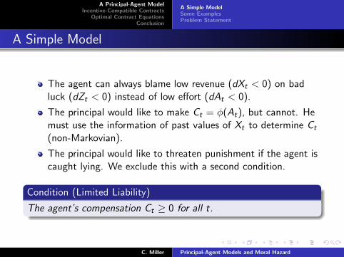
The agent can always blame low revenue (dXt < 0) on badluck (dZt < 0) instead of low effort (dAt < 0).

The principal would like to make Ct = φ(At), but cannot. Hemust use the information of past values of Xt to determine Ct

(non-Markovian).

The principal would like to threaten punishment if the agent iscaught lying. We exclude this with a second condition.

Condition (Limited Liability)

The agent’s compensation Ct ≥ 0 for all t.





Some Examples

Consider a principal owns a farm in the remote countryside andhires an agent to tend to the farm. What are some contracts hecan offer?

1 Ct = c (fixed salary)

2 Ct = aX+t for 0 ≤ a ≤ 1 (share-cropping)

3 Ct = (Xt − c)+ for c ≥ 0 (farming)

Share-cropping and farming are geographically and historicallywidespread. Fixed salary would lead to the agent having noincentive to work.





Some Examples

Moral hazard and limited liability are fundamental to modernfinance industry:

1 Fund managers effort is not easily observable by clients; poorreturns may be blamed on the market (moral hazard)

2 Losses come out of the pocket of the client, not the manager(limited liability)





Problem Statement

Definition

A contract is a pair (Ct ,At), with Ct ≥ 0 and FXt -adapted, while

At is FZt -adapted.

Definition

A contract (Ct ,At) is incentive-compatible (IC) if the effortprocess At maximizes the agent’s total expected utility.





Problem Statement

Definition

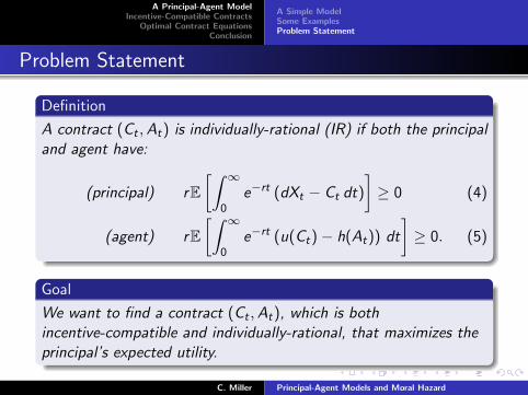
A contract (Ct ,At) is individually-rational (IR) if both the principaland agent have:

(principal) rE[∫ ∞


]≥ 0 (4)

(agent) rE[∫ ∞

0e−rt (u(Ct)− h(At)) dt

]≥ 0. (5)

Goal

We want to find a contract (Ct ,At), which is bothincentive-compatible and individually-rational, that maximizes theprincipal’s expected utility.




Continuation ValueGirsanov TheoremKey Theorem

Continuation Value

Let (Ct ,At) be a contract. We want a characterization of whenthis contract is incentive-compatible. Consider the followingnatural process:

Definition

We define the continuation value the agent derives from followingthe contract (Ct ,At) at time t as:

Wt = rE[∫ ∞

te−r(s−t) (u(Cs)− h(As)) ds | FZ

t

]. (6)

It is useful to derive an SDE governing this process.





Continuation Value

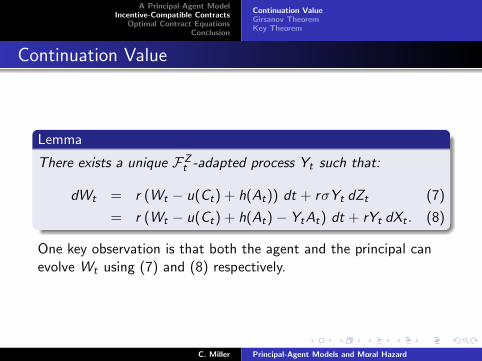
Lemma

There exists a unique FZt -adapted process Yt such that:

dWt = r (Wt − u(Ct) + h(At)) dt + rσYt dZt (7)

= r (Wt − u(Ct) + h(At)− YtAt) dt + rYt dXt . (8)

One key observation is that both the agent and the principal canevolve Wt using (7) and (8) respectively.





Continuation Value

Proof

The idea is to re-write Wt such that a martingale shows up, thenuse the Martingale Representation Theorem. In particular:

Wt = rE[∫ ∞

te−r(s−t) (u(Cs)− h(As)) ds | FZ

t

]= rertE

[∫ ∞0

e−rs (u(Cs)− h(As)) ds | FZt

]−rert

∫ t

0e−rs (u(Cs)− h(As)) ds.





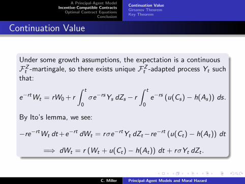
Continuation Value

Under some growth assumptions, the expectation is a continuousFZt -martingale, so there exists unique FZ

t -adapted process Yt suchthat:

e−rtWt = rW0 + r

∫ t

0σe−rsYs dZs − r

∫ t

0e−rs (u(Cs)− h(As)) ds.

By Ito’s lemma, we see:

−re−rtWt dt +e−rt dWt = rσe−rtYt dZt−re−rt (u(Ct)− h(At)) dt

=⇒ dWt = r (Wt + u(Ct)− h(At)) dt + rσYt dZt .





Continuation Value

Next, note that because the agent is assumed to follow thecontract, we have:

Zt =1

σ

(Xt −

∫ t

0As ds

),

so we can replace the dZt in the previous SDE to get:

dWt = r (Wt + u(Ct)− h(At)− YtAt) dt + rYt dXt .





Girsanov Theorem

In the proceeding, we need to consider an alternative effort A∗t .Formally, At and A∗t generate different probability laws for Xt . Wecall them PA and PA∗

respectively. Now we have: ZAt = 1

σ

(Xt −

∫ t0 As ds

)PA-Brownian motion

ZA∗t = 1

σ

(Xt −

∫ t0 A∗s ds

)PA∗

-Brownian motion

related by:

ZA∗t = ZA

t +

∫ t

0

As − A∗sσ

ds. (9)





Girsanov Theorem

Theorem (Girsanov)

Let Zt be a P-Brownian motion and at an adapted process. Definea new process by:

Mt = exp

(∫ t

0as dZs −

1

2

∫ t

0a2s ds

).

If M is uniformly integrable, then a new measure Q, equivalent toP, may be defined by:

dQdP

= M∞.

Furthermore, we have:

Zt −∫ t

0as ds is a Q-Brownian motion.





Key Theorem

Theorem (Characterization of IC Contracts)

A contract (Ct ,At) is IC if and only if

YtAt − h(At) = maxa{aYt − h(a)} a.e. (10)

Proof

First, consider an arbitrary alternative strategy A∗t and the processcorresponding to the return from following A∗t then switching to At :

Vt = r

∫ t

0e−rs (u(Cs)− h(A∗s )) ds + e−rtWt .





Key Theorem

Our goal is to show Vt is a PA∗-submartingale. By Ito’s lemma and

(7):

dVt = re−rt (u(Ct)− h(A∗t )−Wt) dt + e−rt dWt

= re−rt (u(Ct)− h(A∗t )−Wt) dt

+re−rt (Wt − u(Ct) + h(At)) dt

+rσe−rtYt dZAt

= re−rt (h(At)− h(A∗t )) dt + rσe−rtYt dZAt .





Key Theorem

Next, by (9), we rewrite this as:

dVt = re−rt (h(At)− h(A∗t ) + A∗t − At) dt +rσe−rtYt dZA∗t . (11)

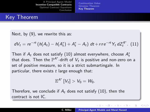
Then if At does not satisfy (10) almost everywhere, choose A∗tthat does. Then the PA∗

-drift of Vt is positive and non-zero on aset of positive measure, so it is a strict submartingale. Inparticular, there exists t large enough that:

EA∗[Vt ] > V0 = W0.

Therefore, we conclude if At does not satisfy (10), then thecontract is not IC.





Key Theorem

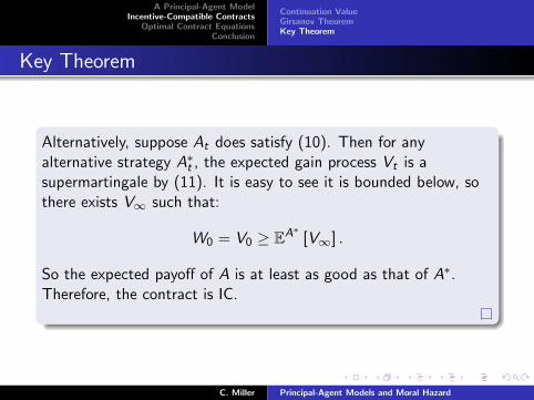
Alternatively, suppose At does satisfy (10). Then for anyalternative strategy A∗t , the expected gain process Vt is asupermartingale by (11). It is easy to see it is bounded below, sothere exists V∞ such that:

W0 = V0 ≥ EA∗[V∞] .

So the expected payoff of A is at least as good as that of A∗.Therefore, the contract is IC.




Control FormulationHamilton-Jacobi Equation

Control Formulation

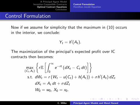
Now if we assume for simplicity that the maximum in (10) occursin the interior, we conclude:

Yt = h′(At).

The maximization of the principal’s expected profit over ICcontracts then becomes:

max(Ct ,At)

{rE[∫ ∞


]}s.t. dWt = r (Wt − u(Ct) + h(At)) + σh′(At) dZt

dXt = At dt + σdZt

W0 = w0, X0 = x0.




Control FormulationHamilton-Jacobi Equation

Hamilton-Jacobi Equation

These notes will be completed for next week...





Date post:	06-Sep-2018
Category:	Documents
Upload:	trinhtram
View:	213 times
Download:	0 times

Principal-Agent Models and Moral Hazardmiller/projects/PrincipalAgentModels.pdf · A...

Documents